Epistemic and Doxastic Planning

Martin Holm Jensen

Kongens Lyngby 2014PhD-2014-316

Technical University of DenmarkDepartment of Applied Mathematics and Computer ScienceMatematiktorvet, Building 303 B, DK-2800 Kongens Lyngby, DenmarkPhone +45 4525 3031compute@compute.dtu.dkwww.compute.dtu.dk

PhD-2014-316

Abstract

This thesis is concerned with planning and logic, both of which are core areasof Artificial Intelligence (AI). A wide range of research disciplines deal withAI, including philosophy, economy, psychology, neuroscience, mathematics andcomputer science. The approach of this thesis is based on mathematics andcomputer science. Planning is the mental capacity that allows us to predict theoutcome of our actions, thereby enabling us to exhibit goal-directed behaviour.We often make use of planning when facing new situations, where we cannotrely on entrenched habits, and the capacity to plan is therefore closely relatedto the reflective system of humans. Logic is the study of reasoning. From certainfixed principles logic enables us to make sound and rational inferences, and assuch the discpline is virtually impossible to get around when working with AI.

The basis of automated planning, the term for planning in computer science,is essentially that of propositional logic, one of the most basic logical systemsused in formal logic. Our approach is to expand this basis so that it is based onricher and and more expressive logical systems. To this end we work with logicsfor describing knowledge, beliefs and dynamics, that is, systems that allow usto formally reason about these aspects. By letting these elements be used in aplanning context, we obtain a system that extends the degree to which goal-directed behaviour can, at present, be captured by automated planning.

In this thesis we concretely apply dynamic epistemic logic to capture knowledge,and dynamic doxastic logic for capturing belief. We highlight two results ofthis thesis. The first pertains to how dynamic epistemic logic can be used todescribe the (lack of) knowledge of an agent in the midst of planning. Thisperspective is already incorporated in automated planning, and seen in isolationthis result appears mainly as an alternative to existing theory. Our second resultunderscores the strength of the first. Here we show how the kinship between theaforementioned logics enable us to extend automated planning with doxasticelements. An upshot of expanding the basis of automated planning is thereforethat it allows for a modularity, which facilitates the introduction of new aspects

ii

into automated planning.

We round things off by describing what we consider to be the absolutely mostfascinating perspective of this work, namely situations involving multiple agents.Reasoning about the knowledge and beliefs of others are essential to act ratio-nally. It enables cooperation, and additionally forms the basis for engaging ina social context. Both logics mentioned above are formalized to deal with mul-tiple agents, and the first steps have been taken towards extending automatedplanning with this aspect. Unfortunately, the first results in this line of researchhave shown that planning with multiple agents is computationally intractable,and additional work is therefore necessary in order to identify meaningful andtractable fragments.

Resumé

Denne afhandling beskæftiger sig med planlægning og logik, der begge er kerne-områder inden for Kunstig Intelligens (KI). En bred vifte af forskningsdisciplinerbehandler KI, herunder bl.a. filosofi, økonomi, psykologi, neurologi, matematikog datalogi. Tilgangen i denne afhandling er funderet i matematikken og data-logien. Planlægning er den mentale evne, som tillader os at forudsige udfaldet afvores handlinger, og herigennem gør os i stand til at udvise målbevidst adfærd.Vi benytter os ofte af planlægning i nye situationer, hvor vi ikke kan forlade ospå indgroede vaner, og evnen til at planlægge er derfor knyttet til mennesketsrefleksive system. Logik er læren om at ræsonnere. Ud fra visse kerneprincippergør logik os i stand til at lave korrekte og rationelle slutninger, og derfor erdisciplinen stort set umulig at komme uden om i arbejdet med KI.

Grundteorien i automatiseret planlægning, den datalogiske betegnelse for plan-lægning, er essentielt bygget på udsagnslogik, hvilket er et af de simpleste syste-mer, der benyttes i den formelle logik. Vores fremgangsmåde er at udvide dennegrundteori, så den baseres på stærkere og mere udtryksfulde logiske systemer.Vi beskæftiger os i den forbindelse med logikker der beskriver viden, overbe-visning og dynamik, dvs. systemer der gør os i stand til formelt at ræsonnereom disse aspekter. Ved at lade disse elementer indgå i en planlægningssammen-hæng opnås en udvidelse af dén målbevidste adfærd, der i dag kan beskrives iautomatiseret planlægning.

Konkret benytter vi i afhandlingen dynamisk epistemisk logik til at beskriveviden, samt dynamisk doksastisk logik til at beskrive overbevisning. Vi fremhæ-ver to resultater fra afhandlingen. Det første drejer sig om, hvordan dynamiskepistemisk logik kan benyttes til at beskrive en aktørs (manglende) viden mensdenne er i gang med planlægge. Dette perspektiv findes allerede inkorporeret iplanlægning, og isoleret set fremstår dette resultat hovedsageligt som et alter-nativ til eksisterende teori. Vores andet resultat fremhæver dog styrken af detførste. Her viser vi, hvordan slægtskabet mellem de to føromtalte logikker gør osi stand til at udvide planlægning med doksatiske elementer. En af styrkerne ved

iv

at løfte grundteorien i planlægning er altså en modularitet, som langt letteretillader indfasning af nye aspekter i automatiseret planlægning.

Vi runder af med at beskrive, hvad vi betragter som det absolut mest fasci-nerende fremtidsperspektiv for dette arbejde, nemlig situationer der omfatterflere aktører. At kunne ræsonnere om andre aktørers viden og overbevisning eressentielt for at kunne agere rationelt. Det er muliggør samarbejde, og dannerderudover grundlaget for at kunne indgå i sociale sammenhænge. Begge logik-ker nævnt ovenfor er formaliseret til at udtale sig om flere aktører, og de førstespadestik er taget til udvidelse af planlægning med dette aspekt. Uheldigvishar de første resultater på dette punkt vist, at planlægning med adskillige ak-tører er beregningsmæssigt fuldstændig uhåndterbart, og yderligere arbejde ernødvendigt for at kunne isolere meningsfyldte fragmenter.

Preface

The work in thesis is a result my PhD study carried out in the section for Al-gorithms, Logic and Graphs in the Department of Applied Mathematics andComputer Science, Technical University of Denmark, DTU. The results pre-sented were obtained in the period from September 2010 to February 2014.My supervisor was Associate Professor Thomas Bolander. In the period fromSeptember 2011 to December 2011 I was on an external research stay at theUniversity of Amsterdam, under the supervision of Alexandru Baltag and Jo-han van Benthem.

This thesis consists of three joint publications and two addenda presenting fur-ther results. It is part of the formal requirements to obtain the PhD degree atthe Technical University of Denmark.

Lyngby, 31-January-2014

Martin Holm Jensen

vi

Acknowledgements

Above all I must thank Thomas Bolander who has been an outstanding super-visor throughout my PhD studies. Thomas has tirelessly guided, advised andeducated me during this period, and I hope that this thesis is able to reflect atleast some of his profound dedication.

I am delighted to have had close collaboration with Mikkel Birkegaard Andersenin much of the work I have done throughout my PhD studies. I must notneglect to mention all of the other great individuals working in the section forAlgorithms, Logic and Graphs at DTU, which have provided for an excellentenvironment both socially and academically. I name a few of the individualswith whom I’ve had fruitful discussions with, which have contributed to thisthesis: Hans van Ditmarsch, Jens Ulrik Hansen, Bruno Zanuttini, Jérôme Lang,Valentin Goranko, Johan van Benthem and Alexandru Baltag. Additionally, Ihighly appreciate the very insightful remarks provided by the members of myassessment committee, which consisted of Valentin Goranko, Andreas Herzigand Thomas Ågotnes.

Lastly, I am indebted and grateful to my dearest Louise for putting up with meduring the final stages of writing this thesis.

viii

Contents

Abstract i

Resumé iii

Preface v

Acknowledgements vii

1 Introduction 11.1 Automated Planning . . . . . . . . . . . . . . . . . . . . . . . . . 2

1.1.1 Automated Planning in Practice . . . . . . . . . . . . . . 71.2 Dynamic Epistemic Logic . . . . . . . . . . . . . . . . . . . . . . 91.3 Epistemic Planning . . . . . . . . . . . . . . . . . . . . . . . . . . 111.4 Related Work . . . . . . . . . . . . . . . . . . . . . . . . . . . . . 131.5 Motivation and Application . . . . . . . . . . . . . . . . . . . . . 161.6 Outline of Thesis . . . . . . . . . . . . . . . . . . . . . . . . . . . 17

2 Conditional Epistemic Planning 21Abstract . . . . . . . . . . . . . . . . . . . . . . . . . . . . . . . . . . . 232.1 Introduction . . . . . . . . . . . . . . . . . . . . . . . . . . . . . . 232.2 Dynamic Epistemic Logic . . . . . . . . . . . . . . . . . . . . . . 252.3 Conditional Plans in DEL . . . . . . . . . . . . . . . . . . . . . . 26

2.3.1 States and Actions: The Internal Perspective . . . . . . . 272.3.2 Applicability, Plans and Solutions . . . . . . . . . . . . . 28

2.4 Plan Synthesis . . . . . . . . . . . . . . . . . . . . . . . . . . . . 312.4.1 Planning Trees . . . . . . . . . . . . . . . . . . . . . . . . 322.4.2 Strong Planning Algorithm . . . . . . . . . . . . . . . . . 382.4.3 Weak Planning Algorithm . . . . . . . . . . . . . . . . . . 39

2.5 Related and Future Work . . . . . . . . . . . . . . . . . . . . . . 40

x CONTENTS

3 Addendum to Conditional Epistemic Planning 433.1 Technical Preliminaries . . . . . . . . . . . . . . . . . . . . . . . . 44

3.1.1 Equivalence . . . . . . . . . . . . . . . . . . . . . . . . . . 443.1.2 Bisimulation . . . . . . . . . . . . . . . . . . . . . . . . . 453.1.3 Size of Inputs . . . . . . . . . . . . . . . . . . . . . . . . . 483.1.4 Model Checking and the Product Update Operation . . . 493.1.5 Types of Planning Problems . . . . . . . . . . . . . . . . . 503.1.6 Alternating Turing Machines and Complexity Classes . . 52

3.2 Suboptimality of StrongPlan(P) . . . . . . . . . . . . . . . . . 553.3 Optimal Decision Procedures . . . . . . . . . . . . . . . . . . . . 59

3.3.1 Replacing Planning Trees . . . . . . . . . . . . . . . . . . 593.3.2 Working with Planning Graphs . . . . . . . . . . . . . . . 633.3.3 Deciding Whether a Solution Exists . . . . . . . . . . . . 673.3.4 Non-Branching Problems . . . . . . . . . . . . . . . . . . 70

3.4 Simulating Turing Machines . . . . . . . . . . . . . . . . . . . . . 723.4.1 Non-branching and Fully Observable Problems . . . . . . 733.4.2 Branching and Fully Observable Problems . . . . . . . . . 793.4.3 Non-branching and Partially Observable Problems . . . . 843.4.4 Branching and Partially Observable Problems . . . . . . . 91

3.5 Conclusion and Discussion . . . . . . . . . . . . . . . . . . . . . . 93

4 Bisimulation for single-agent plausibility models 97Abstract . . . . . . . . . . . . . . . . . . . . . . . . . . . . . . . . . . . 994.1 Introduction . . . . . . . . . . . . . . . . . . . . . . . . . . . . . . 994.2 Single-agent plausibility models and bisimulation . . . . . . . . . 101

4.2.1 Language, structures, and semantics . . . . . . . . . . . . 1014.2.2 Normal epistemic plausibility models and bisimulation . . 1034.2.3 Correspondence between bisimilarity and modal equivalence105

4.3 Degrees of belief and safe belief . . . . . . . . . . . . . . . . . . . 1094.4 Multi-agent epistemic doxastic logic . . . . . . . . . . . . . . . . 1104.5 Planning . . . . . . . . . . . . . . . . . . . . . . . . . . . . . . . . 111

5 Addendum to Bisimulation for single-agent plausibility models1135.1 Degrees of Belief . . . . . . . . . . . . . . . . . . . . . . . . . . . 114

5.1.1 Belief Spheres and the Normal Plausibility Relation . . . 1145.1.2 Bisimulation and Modal Equivalence for LDP . . . . . . . . 116

5.2 Expressive power . . . . . . . . . . . . . . . . . . . . . . . . . . . 1195.2.1 Formalities . . . . . . . . . . . . . . . . . . . . . . . . . . 1205.2.2 Expressive Power of Degrees of Belief . . . . . . . . . . . 1225.2.3 Expressive Power of Safe Belief . . . . . . . . . . . . . . . 125

5.3 Conclusion and Discussion . . . . . . . . . . . . . . . . . . . . . . 126

CONTENTS xi

6 Don’t Plan for the Unexpected: Planning Based on PlausibilityModels 129Abstract . . . . . . . . . . . . . . . . . . . . . . . . . . . . . . . . . . . 1316.1 Introduction . . . . . . . . . . . . . . . . . . . . . . . . . . . . . . 1326.2 Dynamic Logic of Doxastic Ontic Actions . . . . . . . . . . . . . 1336.3 Plausibility Planning . . . . . . . . . . . . . . . . . . . . . . . . . 139

6.3.1 The Internal Perspective On States . . . . . . . . . . . . . 1396.3.2 Reasoning About Actions . . . . . . . . . . . . . . . . . . 1406.3.3 Planning . . . . . . . . . . . . . . . . . . . . . . . . . . . 143

6.4 Plan Synthesis . . . . . . . . . . . . . . . . . . . . . . . . . . . . 1476.4.1 Bisimulations, contractions and modal equivalence . . . . 1486.4.2 Planning Trees . . . . . . . . . . . . . . . . . . . . . . . . 1516.4.3 Planning Algorithm . . . . . . . . . . . . . . . . . . . . . 160

6.5 Related and Future Work . . . . . . . . . . . . . . . . . . . . . . 161

7 Conclusion and Discussion 165

A Proofs 167A.1 Proofs from Section 3.2 . . . . . . . . . . . . . . . . . . . . . . . 167A.2 Proofs from Section 3.3 . . . . . . . . . . . . . . . . . . . . . . . 169A.3 Proofs from Section 3.4 . . . . . . . . . . . . . . . . . . . . . . . 173

Bibliography 179

xii CONTENTS

Chapter 1

Introduction

Artificial intelligence (AI) is a line of research that brings together a vast num-ber of research topics. Indeed, subfields of AI include diverse areas such asphilosophy, mathematics, economics, neuroscience, psychology, linguistics andcomputer science. The ideas and techniques found within this motley crew ofdisciplines have laid the foundation of AI, and, to this day, still contributes to itsfurther development. We can equate the term “artificial” with something thatis man-made, that is, something which is conceived and/or crafted by humans.Pinning down what constitutes “intelligence” is on the other hand a dauntingand controversial task, one which we will not undertake here. Instead we willposit that formal reasoning plays a crucial role in designing and building intelli-gent systems, and that we must require a generality of the reasoning process tosuch an extent that it can be applied to many different types of problems. Thissentiment is our principal motivation for the work conducted in this thesis.

Pertaining more generally to the development of AI, we support the view ofMarvin Minksy that we shouldn’t look for a “magic bullet” for solving all kindsof problems [Bicks, 2010]. In accordance with this stance we make no claimthat the methods presented here are universally best for all tasks. Neverthelesswe find that these methods capture relevant and useful aspects of reasoning, asis also evident from studies in cognitive science (see theory of mind in Section1.5).

We bring up two virtually ubiquitous notions in AI. The first is that of an agent.To us an agent constitutes some entity that is present, and possibly acts, in anenvironment. An agent can represent e.g. a human or a robot acting in theworld, but in general an agent need not have a physical representation and so

2 Introduction

can equally well be a piece of software operating in some environment. Wealso mention environments in which multiple agents are present, each of whichare then taken to represent an individual entity. The second notion is that ofrational agency, which is admittedly more elusive than the first. Following [vanBenthem, 2011] we take rational agency to mean that agents must have someform of rationale behind the choices they make, and that this rationale is basedon an agent’s knowledge, goals and preferences.

In the remainder of this chapter we paint a picture of the topics of AI we treatin this thesis, and along the way point out relationships with results containedin this thesis. We start out with automated planning in Section 1.1, where weexplicate the basic formalism underlying this research discipline. Section 1.2is a brief account of dynamic epistemic logic, a topic we revisit many timesover in later chapters. Following this, Section 1.3 describes what we’ll refer toas epistemic planning, where the theory of the two aforementioned areas cometogether. In Section 1.4 we motivate research into the area of epistemic planningand further discuss a few applications, before we touch upon related formalismsin Section 1.5. We wrap this chapter up in Section 1.6 by outlining the contentsand contributions of subsequent chapters.

1.1 Automated Planning

When planning we want to organize our actions so that in a certain situation,our goal, is brought about. This organization of actions can be representedas a plan for how we should act. By predicting the outcome of the actions atour disposal, we have a method for generating plans that lead us to our goal.In the textbook [Ghallab et al., 2004] planning is called the “reasoning side ofacting”, meaning that it constitutes a process of careful deliberation about thecapabilities we’re endowed with. The following presentation is mainly basedon [Ghallab et al., 2004], though we fill in some blanks using the thoroughexposition of planning due to [Rintanen, 2005]. Our aim is to give the reader afeel for the theory underlying automated planning, while keeping notation andlong-winded digressions to a minimum.

Our point of departure is what constitutes the simplest form of planning prob-lem. In this case we consider three components: An initial state, a set of actions(an action library) and a goal, with each of these being represented using simplenotions from set theory. In this set-theoretic formulation we take a finite set ofsymbols P . A state is taken to be a subset of P , and we let actions manipulatestates by removing and/or adding symbols. A goal is a collection of states (asubset of the powerset of P ). The intuition is that a symbol p ∈ P is true in a

1.1 Automated Planning 3

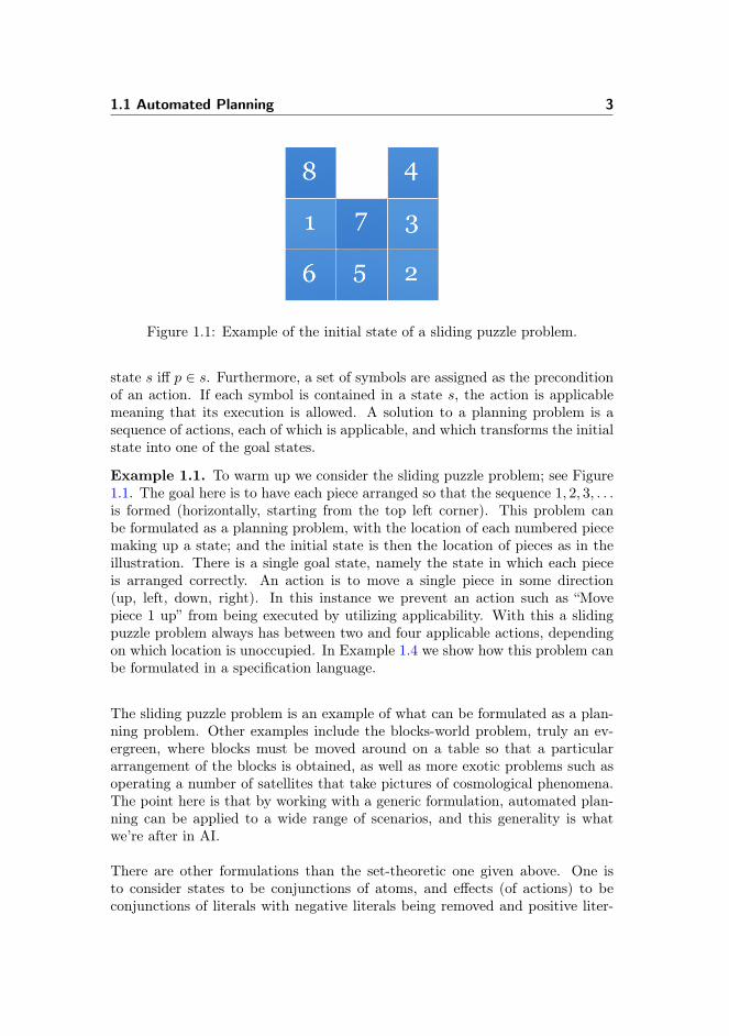
Figure 1.1: Example of the initial state of a sliding puzzle problem.

state s iff p ∈ s. Furthermore, a set of symbols are assigned as the preconditionof an action. If each symbol is contained in a state s, the action is applicablemeaning that its execution is allowed. A solution to a planning problem is asequence of actions, each of which is applicable, and which transforms the initialstate into one of the goal states.

Example 1.1. To warm up we consider the sliding puzzle problem; see Figure1.1. The goal here is to have each piece arranged so that the sequence 1, 2, 3, . . .is formed (horizontally, starting from the top left corner). This problem canbe formulated as a planning problem, with the location of each numbered piecemaking up a state; and the initial state is then the location of pieces as in theillustration. There is a single goal state, namely the state in which each pieceis arranged correctly. An action is to move a single piece in some direction(up, left, down, right). In this instance we prevent an action such as “Movepiece 1 up” from being executed by utilizing applicability. With this a slidingpuzzle problem always has between two and four applicable actions, dependingon which location is unoccupied. In Example 1.4 we show how this problem canbe formulated in a specification language.

The sliding puzzle problem is an example of what can be formulated as a plan-ning problem. Other examples include the blocks-world problem, truly an ev-ergreen, where blocks must be moved around on a table so that a particulararrangement of the blocks is obtained, as well as more exotic problems such asoperating a number of satellites that take pictures of cosmological phenomena.The point here is that by working with a generic formulation, automated plan-ning can be applied to a wide range of scenarios, and this generality is whatwe’re after in AI.

There are other formulations than the set-theoretic one given above. One isto consider states to be conjunctions of atoms, and effects (of actions) to beconjunctions of literals with negative literals being removed and positive liter-

4 Introduction

als being added. In this formulation we can immediately see a connection topropositional logic, though often the relationship between logic and automatedplanning is much less evident. The seminal [Fikes and Nilsson, 1971], whichintroduced the generic problem solver “STRIPS” (STanford Research InstituteProblem Solver), used a much more expressive formulation of planning, includ-ing the ability to use arbitrary formulas of first-order logic as effects. As itturned out to be hard to give well-defined semantics for this formulation, thecompromise based on propositional logic was adopted [Ghallab et al., 2004].

Underlying our presentation in the above are several assumptions about theenvironment. It is fully observable as a symbol is known to be either true orfalse; it is deterministic as the execution of an action brings the environment to asingle other state; and it is static as only the planning agent brings about changeto the environment. The reasoning (or, planning) process is offline meaning thatonly when the agent acts is the environment modified, and so there is no needfor interleaving of planning and execution. The type of planning that falls underthese restrictions is often referred to as as classical planning.

Already present in classical planning is the important distinction between plan-time and run-time. The former is when the planning agent is deliberating aboutwhat course of action it must take to achieve its goal, and the latter is whena plan is actually executed. This distinction becomes crucial as we now turnto environments with partial observability and nondeterminism, by relaxingsome of the assumptions of classical planning. The general formulation in au-tomated planning is based on Partially Observable Markov Decision Processes(POMDPs), meaning that both observations and actions are assigned probabil-ity distributions and so this leads to an inherently stochastic environment. Asa consequence of this choice of modelling, when treating environments that arenondeterministic and partially observable yet not stochastic, automated plan-ning employs a non-probabilistic form of POMDPs.

Partial observability leads to the notion of a belief state (a set of states; i.e.subset of 2P ), which signifies that what is known is only that one state in abelief state is, or will be, the actual situation.1 There are various approaches

1There is actually an important remark about our use of the future continuous form willbe here. We use it to underscore that we’re in the midst of a reasoning process (plan-time),and so it seems to indicate a future situation that just hasn’t happened yet. However, exactlybecause we’re in a deliberation phase, this particular future can only come about should theagent choose to act in a particular way. Even still, due to the nondeterministic nature ofthe environment it may not be possible for the agent to determine (at plan-time), whetherthis future situation is going to be realized at all. On top of this, the agent may also beignorant about certain facts, and so what we’re trying to convey here contains several layersof intricacy. Rather than canvassing for a grammatically more accurate statement, we’ll stickwith the future continuous form and let the precise meaning be deduced from the mathematicalframework in question.

1.1 Automated Planning 5

to how belief states are induced, that is, when two states are considered indis-tinguishable to the agent. One method is to use a set of observation variablesV ⊆ P , denoting exactly the propositions whose truth value can be observed atrun-time. These variables are automatically observed after each action, whilethe truth value of variables in P \V can never be determined by the agent. Non-determinism is handled by allowing actions to manipulate states in more thanone way, so, for instance, an action may or may not add a proposition symbolto a state. One result from this choice of modelling is that observability andnondeterminism are completely detached from one another; actions still manip-ulate states (not belief states) and observation variables are statically given andindependent of actions. We should note that [Rintanen, 2005, Section 4.1.1]shows how this representation is able to express observing the truth of arbitrarypropositional formulas over P upon the execution of a particular action (referredto as sensing actions).

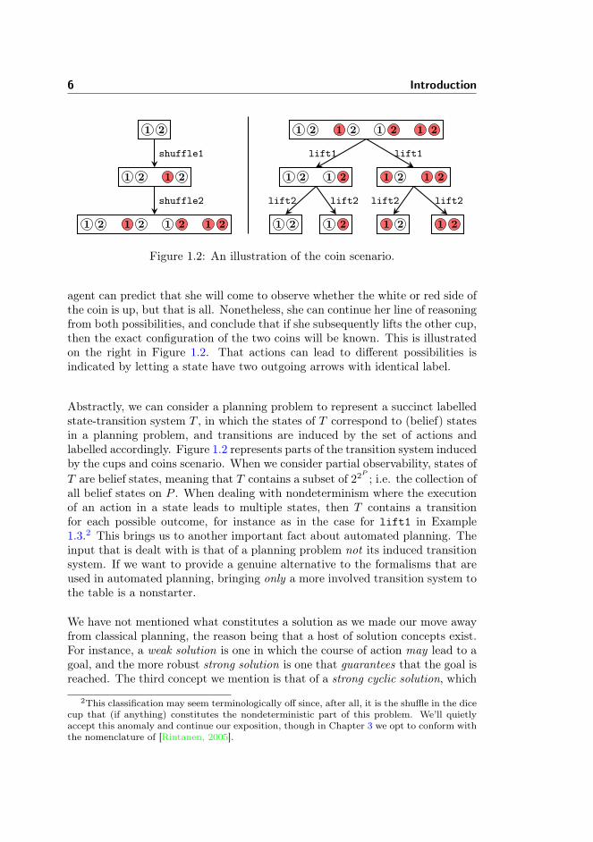
Example 1.2. Consider an agent having two dice cups and two coins (named 1and 2) both of which have a white side and red side. She can shuffle a coin usinga dice cup thereby leaving which side comes up top concealed, and she can lifta cup and observe the top facing color of a concealed coin. In this scenario wetake a state to be the top facing color of both coins. Further, her action libraryconsists of the actions that represent shuffling the coins and lifting the cups.Say now that in the initial state the two coins are showing their white side, andthat neither are hidden by a cup. If the agent shuffles coin 1, the result is thatshe’ll still know that coin 2 is showing its white side, but not whether it is thewhite or red side of coin 1 that is up. If she subsequently shuffles coin 2, theresult is that both coins are concealed by a cup and she is ignorant about whichside is up on either coin. This is illustrated on the left in Figure 1.2, where weuse arrows to indicate actions and rectangles to indicate belief states.

Here the agent is able to fully predict what will happen, at least from her ownperspective, where she will become ignorant about which sides of the coins areup. Of course, and this is a fair point, there is some actual configuration of thecoins, but in planning we take on the role of a non-omniscient agent and modelthings from this perspective.

When working with belief states, we need to rephrase the notion of applicability.Given a belief state, an action is applicable if its precondition is satisfied inevery state in the belief state. This is motivated by the sentiment, that if theprecondition of an action is not satisfied in some state, then the agent has noway of predicting what happens, hence this is disallowed. Arguably, we caninterpret this as modicum of rational agency, because it reflects the disinterestof the agent to act in a manner that makes her knowledge inconsistent.

Example 1.3. We continue the cups and coins scenario where we left off, andnow consider the case of lifting the dice cup concealing coin 1. At plan-time the

6 Introduction

1 2

1 2 1 2

1 2 1 2 1 2 1 2

shuffle1

shuffle2

1 2 1 2 1 2 1 2

1 2 1 2 1 2 1 2

1 2 1 2 1 2 1 2

lift1 lift1

lift2 lift2 lift2 lift2

Figure 1.2: An illustration of the coin scenario.

agent can predict that she will come to observe whether the white or red side ofthe coin is up, but that is all. Nonetheless, she can continue her line of reasoningfrom both possibilities, and conclude that if she subsequently lifts the other cup,then the exact configuration of the two coins will be known. This is illustratedon the right in Figure 1.2. That actions can lead to different possibilities isindicated by letting a state have two outgoing arrows with identical label.

Abstractly, we can consider a planning problem to represent a succinct labelledstate-transition system T , in which the states of T correspond to (belief) statesin a planning problem, and transitions are induced by the set of actions andlabelled accordingly. Figure 1.2 represents parts of the transition system inducedby the cups and coins scenario. When we consider partial observability, states ofT are belief states, meaning that T contains a subset of 22P

; i.e. the collection ofall belief states on P . When dealing with nondeterminism where the executionof an action in a state leads to multiple states, then T contains a transitionfor each possible outcome, for instance as in the case for lift1 in Example1.3.2 This brings us to another important fact about automated planning. Theinput that is dealt with is that of a planning problem not its induced transitionsystem. If we want to provide a genuine alternative to the formalisms that areused in automated planning, bringing only a more involved transition system tothe table is a nonstarter.

We have not mentioned what constitutes a solution as we made our move awayfrom classical planning, the reason being that a host of solution concepts exist.For instance, a weak solution is one in which the course of action may lead to agoal, and the more robust strong solution is one that guarantees that the goal isreached. The third concept we mention is that of a strong cyclic solution, which

2This classification may seem terminologically off since, after all, it is the shuffle in the dicecup that (if anything) constitutes the nondeterministic part of this problem. We’ll quietlyaccept this anomaly and continue our exposition, though in Chapter 3 we opt to conform withthe nomenclature of [Rintanen, 2005].

1.1 Automated Planning 7

is guaranteed to eventually lead to the goal. In Chapter 6 we propose a solutionconcept based on qualitative plausibilities, which positions itself somewhere inbetween weak and strong solutions.

With this we hope to have left the reader with some semblance of what auto-mated planning is all about. Next we complement what we presented above bydescribing briefly the empiric basis of automated planning, which is a side toautomated planning that shouldn’t be overlooked.

1.1.1 Automated Planning in Practice

There are many implementations of planning systems in existence, and competi-tions are held in tandem with the International Conference on Automated Plan-ning and Scheduling (ICAPS), where these systems can be empirically evaluatedon a wide range of planning problems. Problems are not formulated as presentedhere, but rather using the Planning Domain Definition Language (PDDL) orig-inating with [Ghallab et al., 1998]. PDDL is a lifted representation of planningproblems, based on a typed first-order language with a finite number of predi-cates and constants, and without functions. By grounding this language we canobtain a planning problem in the set-theoretic formulation given above. Thefull details are beyond our scope, but the following example serves to illustratethe connection.

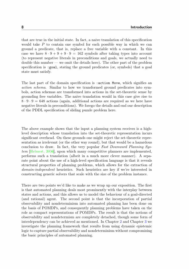
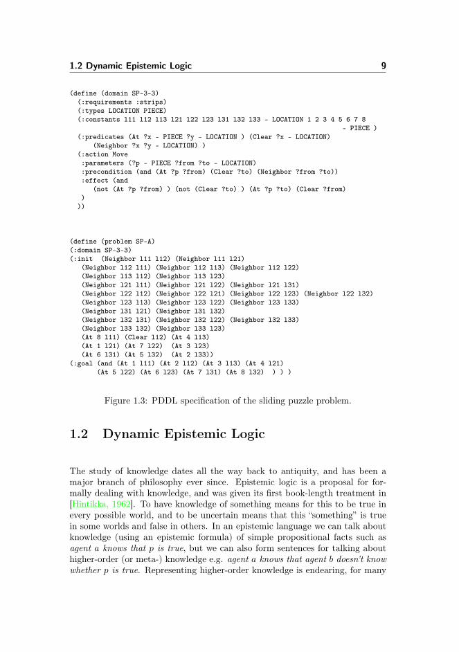
Example 1.4. In Figure 1.3 we show how the sliding puzzle problem in Example1.1 can be specified using PDDL. A planning problem is formulated from adomain specification and a problem specification. The domain specification setsthe rules for the planning problem, and the problem instance determines whereto start from and where to go.

We start out with the domain specification at the top of Figure 1.3. Here the:constants represent locations and pieces, and each constant is assigned a type,which can be seen as an implicit unary predicate. In :predicates we specifythe predicates for giving meaning to constants. Writing ?x indicates a freevariable that is eligible for substitution with a constant. We use At to indicatethe location of a piece, Clear to specify the location which is unoccupied, andNeighbor for encoding the geometry of the puzzle. Before discussing actions,we turn to the the problem specification.

At the bottom of Figure 1.3 is the problem specification. Here :init specifiesthe initial state of the planning problem by listing a number of ground predicatessuch as (At 8 l11). Taking each ground predicate to be a symbol in P (as usedin the set-theoretic formulation), we can see :init as specifying the symbols

8 Introduction

that are true in the initial state. In fact, a naive translation of this specificationwould take P to contain one symbol for each possible way in which we canground a predicate, that is, replace a free variable with a constant. In thiscase we have 8 · 9 + 9 + 9 · 9 = 162 symbols after taking types into account(to represent negative literals in preconditions and goals, we actually need todouble this number — we omit the details here). The other part of the problemspecification is :goal, stating the ground predicates (or, symbols) that a goalstate must satisfy.

The last part of the domain specification is :action Move, which signifies anaction schema. Similar to how we transformed ground predicates into sym-bols, action schemas are transformed into actions in the set-theoretic sense bygrounding free variables. The naive translation would in this case give rise to8 · 9 · 9 = 648 actions (again, additional actions are required as we here havenegative literals in preconditions). We forego the details and end our descriptionof the PDDL specification of sliding puzzle problem here.

The above example shows that the input a planning system receives is a high-level description whose translation into the set-theoretic representation incurssignificant overhead. On these grounds one might reject the set-theoretic repre-sentation as irrelevant (or the other way round), but that would be a hazardousconclusion to draw. In fact, the very popular Fast Downward Planning Sys-tem [Helmert, 2006], upon which many competitive planners are implemented,performs such a translation (albeit in a much more clever manner). A sepa-rate point about the use of a high-level specification language is that it revealsstructural properties of planning problems, which allows for the extraction ofdomain-independent heuristics. Such heuristics are key if we’re interested inconstructing generic solvers that scale with the size of the problem instance.

There are two points we’d like to make as we wrap up our exposition. The firstis that automated planning deals most prominently with the interplay betweenstates and actions, and this allows us to model the behaviour of a goal-directed(and rational) agent. The second point is that the incorporation of partialobservability and nondeterminism into automated planning has been done onthe basis of POMDPs, and consequently planning problems have taken on therole as compact representations of POMDPs. The result is that the notions ofobservability and nondetermism are completely detached, though some form ofinterdependency can be achieved as mentioned. In Chapter 2 and Chapter 3 weinvestigate the planning framework that results from using dynamic epistemiclogic to capture partial observability and nondeterminism without compromisingthe basic principles of automated planning.

1.2 Dynamic Epistemic Logic 9

(define (domain SP-3-3)(:requirements :strips)(:types LOCATION PIECE)(:constants l11 l12 l13 l21 l22 l23 l31 l32 l33 - LOCATION 1 2 3 4 5 6 7 8

- PIECE )(:predicates (At ?x - PIECE ?y - LOCATION ) (Clear ?x - LOCATION)

(Neighbor ?x ?y - LOCATION) )(:action Move:parameters (?p - PIECE ?from ?to - LOCATION):precondition (and (At ?p ?from) (Clear ?to) (Neighbor ?from ?to)):effect (and

(not (At ?p ?from) ) (not (Clear ?to) ) (At ?p ?to) (Clear ?from))

))

(define (problem SP-A)(:domain SP-3-3)(:init (Neighbor l11 l12) (Neighbor l11 l21)

(Neighbor l12 l11) (Neighbor l12 l13) (Neighbor l12 l22)(Neighbor l13 l12) (Neighbor l13 l23)(Neighbor l21 l11) (Neighbor l21 l22) (Neighbor l21 l31)(Neighbor l22 l12) (Neighbor l22 l21) (Neighbor l22 l23) (Neighbor l22 l32)(Neighbor l23 l13) (Neighbor l23 l22) (Neighbor l23 l33)(Neighbor l31 l21) (Neighbor l31 l32)(Neighbor l32 l31) (Neighbor l32 l22) (Neighbor l32 l33)(Neighbor l33 l32) (Neighbor l33 l23)(At 8 l11) (Clear l12) (At 4 l13)(At 1 l21) (At 7 l22) (At 3 l23)(At 6 l31) (At 5 l32) (At 2 l33))

(:goal (and (At 1 l11) (At 2 l12) (At 3 l13) (At 4 l21)(At 5 l22) (At 6 l23) (At 7 l31) (At 8 l32) ) ) )

Figure 1.3: PDDL specification of the sliding puzzle problem.

1.2 Dynamic Epistemic Logic

The study of knowledge dates all the way back to antiquity, and has been amajor branch of philosophy ever since. Epistemic logic is a proposal for for-mally dealing with knowledge, and was given its first book-length treatment in[Hintikka, 1962]. To have knowledge of something means for this to be true inevery possible world, and to be uncertain means that this “something” is truein some worlds and false in others. In an epistemic language we can talk aboutknowledge (using an epistemic formula) of simple propositional facts such asagent a knows that p is true, but we can also form sentences for talking abouthigher-order (or meta-) knowledge e.g. agent a knows that agent b doesn’t knowwhether p is true. Representing higher-order knowledge is endearing, for many

10 Introduction

of our every-day inferences are related to the knowledge of others (we discussthe notion of a theory of mind in Section 1.5).

The notion of knowledge can be formally given with regards to a relationalstructure, consisting of a set of possible worlds along with a set of accessibilityrelations (one for each agent) on this set of possible worlds. We add to thisa valuation, assigning to each world the basic propositional symbols (such asp) that are true, and we call the result an epistemic model. Statements aboutknowledge, such as those given above, are then interpreted on epistemic mod-els, with basic facts such as p being determined from the valuation in a world,and (higher-order) knowledge being determined from the interplay between theaccessibility relations and the valuation. As epistemic models are formally pre-sented already in Chapter 2 we refrain from providing further details at thispoint.

Example 1.5. We now return to the coin scenario, and discuss how the beliefstates in automated planning are related to single-agent epistemic models. Wecan think of each state in a belief state as representing a possible world. If wefurther assume that the accessibility relation of an epistemic model is univer-sal, then what is known in a belief state coincides with the interpretation ofknowledge as truth in every possible world. Belief states therefore capture acertain, idealized, version of knowledge in the single-agent case. Taking on thisview, each rectangle illustrated in Figure 1.2 represents a single-agent epistemicmodel, and so this establishes the first simple connection between automatedplanning and epistemic logic.

What is missing is how to capture the actions in automated planning is a dy-namic component. Fortunately, the idea of extending epistemic logic with dy-namic aspects has been investigated to a great extent over the past severaldecades. In [Fagin et al., 1995] (the culmination of a series of publications bythe respective authors) it is shown how the analysis of complex multi-agent sys-tems benefits from ascribing knowledge to agents, with an emphasis on its usein computer science. That epistemic logic, based on questions posed in ancienttimes, would come into the limelight of computer science demonstrates just howall-pervasive the notion of knowledge is.

One extension of epistemic logic that deals with dynamics of information is [Bal-tag et al., 1998], often referred to as the “BMS” framework. What is so appealingabout this framework is that it can represent a plethora of diverse dynamics,such as obtaining hard evidence, being misinformed, or secretly coming to knowsomething other agents do not. As such the framework is inherently multi-agent,though for the most part we consider the single-agent version. The presentationwe give in Chapter 2 is due to [van Ditmarsch and Kooi, 2008] which allows forfactual (or ontic) change. We’ll refer to this as dynamic epistemic logic (DEL),

1.3 Epistemic Planning 11

even though several logics not based on the BMS framework adhere to thisdesignation. The dynamic component of DEL is introduced via event models,sometimes called actions models or update models. The dynamics is by virtueof the product update operation, in which event models are “multiplied” withepistemic models by taking a restricted Cartesian product of the two structuresto form a new epistemic model. On the basis of Example 1.5 we can see eventmodels as a method for transforming one belief state into another — exactly thepurpose of actions in automated planning as discussed above. This relationshipbetween event models and actions of automated planning was pointed out in[Löwe et al., 2011, Bolander and Andersen, 2011].

We can assure the reader that we will be dealing both with DEL and relatedtopics in the ensuing chapters, and so we close our discussion after a digressionconcerning modal logic. The purpose of modal logic (or, modal languages) is totalk about relational structures, namely by its use of Kripke semantics. Kripkesemantics coincides with truth in every possible world which we use to ascribeknowledge to an agent, but it can also be used to describe modalities of belief (aweaker form of knowledge), time or morality [Blackburn et al., 2001]. Epistemiclogic is therefore a subfield of modal logic, and there is a cross-fertilization ofideas between the two areas, and in many cases results from modal logic carryover directly to epistemic logic. The first point is evident from the investigationof dynamic modal logic in the 1980s which later played a role in developmentof DEL. The second point is evident as results from modal model theory, forinstance those concerning the notion of bisimulation, also plays a fundamentalrole in the model theory of epistemic models [van Ditmarsch et al., 2007].

1.3 Epistemic Planning

One of the points in Section 1.1 is that automated planning problems are givenas an initial state, a number of actions and a goal. In our investigation ofplanning we take this to be our starting point. What we’re after are approachesthat extend the foundation of automated planning, in particular by making useof richer logics; e.g. modal logics. Epistemic planning is one such approach andhere the richer logic is DEL, which was seminally, and independently, taken in[Löwe et al., 2011, Bolander and Andersen, 2011]. Later works include [Andersenet al., 2012] (the extended version of which constitutes Chapter 2), as well as[Yu et al., 2013, Aucher and Bolander, 2013].

In epistemic planning the initial state is an epistemic model, actions are a num-ber of event models and a goal is an epistemic formula. In [Bolander and Ander-sen, 2011] the solution to a problem is to find a sequence of event models which,

12 Introduction

using the product update operation, produces an epistemic model satisfying thegoal formula. The authors show this problem to be decidable for single-agentDEL, but undecidable for multi-agent DEL. In [Löwe et al., 2011] some tractablecases of multi-agent epistemic planning are provided. While their approach doesnot consider factual change, their notion of a solution does coincide with [Bolan-der and Andersen, 2011] to the extent that both consider plans as sequences ofevent models. Recently [Aucher and Bolander, 2013] showed that multi-agentepistemic planning is also undecidable without factual change, while [Yu et al.,2013] identified a fragment of multi-agent epistemic planning that is decidable.

Automated planning deals with a single agent environment (depending on whetherwe interpret nature as an agent), and in this sense each of the aforementionedapproaches appear to be immediate generalizations. Here we must make certainreservations. First, with the exception of [Bolander and Andersen, 2011] noneof these approaches cater to applicability as described previously. As such, themodicum of rational agency we interpreted from an agent’s interest in havingconsistent knowledge is absent in these presentations. The interpretation in [Yuet al., 2013] is in this sense more appropriate, since it phrases the problem asexplanatory diagnosis, meaning that the sequence of event models produced rep-resent an explanation of how events may have unfolded, when the “knowledgestate” of the system satisfies some epistemic formula (called an observation).We also treat this point in Chapter 2 as the question of an internal versus ex-ternal perspective. Second, while the formalisms deal with the knowledge ofmultiple agents, individual autonomous behaviour is not considered. Obviously,automated planning does not provide a solution to these multi-agent aspects,but we do consider it to embody autonomous behaviour of a single agent, and sobelieve multi-agent planning should deal with each agent exhibiting autonomousbehaviour. Third, as solutions are sequences of plans, formalizing notions suchas a weak solution or a strong solution are difficult, because they require theagent to make choices as the outcome of actions unfold; e.g. on the basis of whatis observed as the coin is lifted in Example 1.3.3 Chapter 2 extends single-agentepistemic planning with a plan language to tackle this third point.

We point out two references that, in spite of their endearing titles, do notconform to what we take to constitute epistemic planning. The first is “DEL-sequents for regression and epistemic planning” [Aucher, 2012]. Slightly simpli-fied, the problem of epistemic planning is here formulated as finding a singleevent model (with certain constraints) that produces, from a given epistemicmodel (initial state), an epistemic model satisfying an epistemic formula (goal).Missing here is that this single event model, while built from atomic events,does not necessarily represent any single action (or sequence of actions) of the

3[Bolander and Andersen, 2011] proposes to internalize branching in the event models,implying an extensive modification of the action library. Capturing both weak and strongsolution concepts using this approach appears difficult.

1.4 Related Work 13

action library. The second is “Tractable Multiagent Planning for EpistemicGoals” [van der Hoek and Wooldridge, 2002]. Here the problem that is solved isnot finding a solution when given an initial state, an action library and a goal;rather it is finding a solution when given the underlying transition system ofsuch a planning problem. While the promises of tractability are intriguing, itis important to note that this is in terms of the size of the transition system.Furthermore, the transition system is assumed finite which we generally cannotassume in our reading of epistemic planning. In both cases the problems treatedare shown to be decidable, which is not compatible with the results of [Bolanderand Andersen, 2011].

1.4 Related Work

At the end of each chapter, we discuss work related to the topics that arecovered. Our aim now is to provide a broader perspective on things by discussingrelated approaches for dealing with actions, knowledge, autonomous behaviourand rational agency.

One profound investigation of multi-agent planning is [Brenner and Nebel, 2009],which situates multiple autonomous agents in a dynamic environment. In thissetting agents have incomplete knowledge and restricted perceptive capabilities,and to this end each agent is ascribed a belief state. These belief states are basedon multi-valued state-variables, which allows for a more sophisticated versionof belief state than that discussed in Section 1.1. In a slightly ad-hoc manner,agents can reason about the belief states of other agents. For instance inferringthat another agent has come to know the value of a state-variable due to anobservation, or by forming mutual belief in the value of a state-variable usingspeech acts. The authors apply their formalism experimentally, modelling anumber of agents operating autonomously in a grid world scenario. We wouldlike to see what could be modelled in this framework when introducing epistemicmodels as the foundation of each agent’s belief state.

We already mentioned the approach of [van der Hoek and Wooldridge, 2002],which more generally pertains to the planning as model checking paradigm.Other cognates are [Cimatti et al., 2003, Bertoli et al., 2001], where symbolicmodel checking techniques are employed, which allows for compactly represent-ing the state-transition system. Indeed, in some cases the representation of abelief state as a propositional formula is exponentially more succinct. Moreover,it is possible to compute the effects of multiple actions in a single step. As such,this line of research, also used for much richer logics, may prove key to theimplementation of efficient planners for planning with more expressive logics.

14 Introduction

On the topic of expressive logics, we bring up formalisms that deal with thebehaviour of agents over time. Two such logical systems are epistemic temporallogic (ETL) [Parikh and Ramanujam, 2003] and the interpreted systems (IS)of [Fagin et al., 1995], which in [Pacuit, 2007] are shown to be modally equiva-lent for a language with knowledge, next and until modalities. Under scrutinyin ETL/IS are structures that represent interactive situations involving multi-agents, and may be regarded as a tool for the analysis of social situations, albeitsimilar to how computation is described using machine code [Pacuit, 2007]. ETLuses the notion of local and global histories. A global history represents a se-quence of events that may take place, and local histories result from projectingglobal histories to the vantage point of individual agents, subject to what eventsagents are aware of.

[van Benthem et al., 2007] investigates a connection between ETL and DEL,interpreting a sequence of public announcements (a special case of event models)as the temporal evolution of a given initial epistemic model. These sequences ofpublic announcements are constrained so that they conform to a given protocol.The main result is the characterization of the ETL models that are generatedby some protocol. Imagining protocols that allow for a more general form ofevent model and that further capture applicability, we would to a great extentbe within the framing of epistemic planning, and one step nearer to mappingout a concrete relationship between the two approaches.

There are even richer logics for reasoning about agents and their group capabil-ities, such as Coalition Logic [Pauly, 2002], ATL [Alur et al., 2002] and ATEL[van der Hoek and Wooldridge, 2002]. An extensive comparison of all three is[Goranko and Jamroga, 2004], which also presents methods for transforming be-tween the various types of models and languages involved, and further notes theclose relationship between lock-step synchronous alternating transition systemsand interpreted systems. A characterization of these structures in terms of (se-quences of) event models is an interesting yet, to our knowledge, unprobed area.Related is also the concept of “Seeing-to-it-that” (STIT) [Belnap et al., 2001],emanating as a formal theory for clarifying questions in the philosophy of actionand the philosophy of norms. Over the past decade most work on STIT theoryhas been within the field of computer science, for instance by providing resultson embedding fragments of STIT logic into formalisms akin to those mentionedin this paragraph [Bentzen, 2010, Broersen et al., 2006a]. A non-exhautive listis [Schwarzentruber and Herzig, 2008, Herzig and Lorini, 2010, Broersen et al.,2006b]. As pointed out in [Benthem and Pacuit, 2013], research into logics ofagency has seen a shift from being a “Battle of the Sects” to an emphasis onsimilarities and relative advantages of the various paradigms. Getting epistemicplanning aboard this train might be a pathway towards a multi-agent planningframework dealing with both individual and collective agency.

1.4 Related Work 15

The work in [Herzig et al., 2003] is close to single-agent epistemic planning.Their complex knowledge states are given syntactically, and represent a setof S5 Kripke models. They introduce ontic actions and epistemic actions asseparate notions. The ontic action language is assumed to be given in thesituation calculus tradition, so that actions must specify what becomes true attime t + 1 based on what is true at time t. An epistemic action is given asa set of possible outcomes; each possible outcome is a propositional formulathat represents what the agent comes to know should the particular observationoccur. Progression of actions (or, the projection of possible outcomes), andsubsequently plans, is given by syntactic manipulation of complex knowledgestates. As recently shown in [Lang and Zanuttini, 2013], this approach allowsfor an exponentially more compact representation of plans; the cost comes atexecution time where the evaluation of branching formulas is not constant-time.We recently showed how progression of both epistemic actions and ontic actionscan be expressed as event models [Jensen, 2013b], providing insight into therelationship between this approach and single-agent epistemic planning. Thereseems to be no perspicuous method for extending progression in this frameworkto a multi-agent setting. Because of this we find DEL and its product updateoperation to be much more enticing.

An extension of the approach mentioned in the previous paragraph is [Lavernyand Lang, 2004] and [Laverny and Lang, 2005]. Here the purely epistemicapproach is extended with graded beliefs, that is, belief in some formula to acertain degree. Belief states (as they are, in this context, confusingly called)are introduced via the ordinal conditional functions (or, kappa functions) dueto [Spohn, 1988]. What this allows for is modeling scenarios in which an agentreasons about its current beliefs, but more importantly, its future beliefs subjectto the actions it can execute. This is similar to our work in Chapter 6, thoughthere are some conceptual differences, with one being (again) that the actionlanguage used has no immediate multi-agent counterpart. Another is that intheir approach, plans dealing with the same contingency many times over (e.g.a plan that replaces a light bulb, and, in case the replacement is broken, replacesit again — cf. Example 6.1) have a higher chance of success than plans that donot, something which our approach does not naturally handle. There are othernon-trivial connections between our approach and that of Laverny and Lang,and further investigation seems prudent.4

We end this section by mentioning the “Planning with Knowledge and Sensingplanning system” (PKS) due to [Petrick and Bacchus, 2002, Petrick and Bac-chus, 2004]. PKS is an implementation of a single-agent planning system usingthe approach of explicitly modeling the agent’s knowledge. The argument is, as

4I thank Jérôme Lang for bringing these frameworks to my attention, as well as making adiligent comparison to the work in Chapter 6.

16 Introduction

is also stressed in [Bolander and Andersen, 2011], that this is a more naturaland general approach to partial observability than variants using e.g. observa-tion variables. An agent’s knowledge is compromised of four databases, each ofwhich can be translated to a collection of formulas in epistemic logic (with somefirst-order extensions), and actions are modelled by modifying these databasesseparately. They concede that certain configurations of epistemic models cannotbe captured, one effect being that their planning algorithm is incomplete. Theirargument is pragmatic and PKS was capable of solving then contemporary plan-ning problems. What PKS represents is the bottom-up approach to epistemicplanning, taking a fragment of epistemic logic as the basis for extending classicalplanning to handle partial observability.

1.5 Motivation and Application

The goal of the Joint Action for Multimodal Embodied Social Systems (JAMES)project is to develop an artificial embodied agent that supports socially appro-priate, multi-party, multimodal interaction [JAMES, 2014]. As such it combinesmany different disciplines belonging to AI, including planning with incompleteinformation. Concretely, the project considers a robot bartender (agent) thatmust be able to interact socially intelligent with patrons. Actions available in-clude asking for a drink order and serving it, which requires the generation ofplans for obtaining information. This is done in an extension of the PKS frame-work we described above, which replans when knowledge is not obtained (e.g.the patron mumbles when ordering) or when knowledge is obtained earlier thanexpected (eg. the patron orders prior to being asked). The social component isin the ability to understand phrases such as “I’ll have the same as that guy” or“I’ll have another one”, which requires a model of each patron. Moreover, therobot bartender must be able to comprehend social norms, for instance when aperson asks for five drinks and four bystanders are ignoring it, then it shouldplace the drinks in front of each individual.5

While the robot bartender gets by with considering each patron separately, notall social situations are as lenient. We find evidence for this within cognitivescience, more specifically in the concept of a theory of mind [Premack andWoodruff, 1978]. Theory of mind refers to a mechanism which underlies a crucialaspect of social skills, namely that of being able to conceive of mental states,including what other people know, want, feel or believe. [Baron-Cohen et al.,1985] subjected 61 children to a false-belief task, where each child observed apretend play involving two doll protagonists Sally and Anne. The scenario isthat Sally places a marble in a basket, leaves the scene, after which Anne tranfers

5These remarks are based on personal communication with Ron Petrick.

1.6 Outline of Thesis 17

the marble to a box. As Sally returns to the scene, the child is asked whereSally will look for her marble (a belief question), and additionally where themarble really is (a reality question). The children were divided into three groups,namely as either being clinically normal, affected by Down’s syndrome or autistic(as determined by a previous test). The passing rate for the belief question(whose correct answer is the basket) for both clinically normal and Down’ssyndrome children was respectively 85% and 86%, whereas the failure rate forthe autistic group was 80%. At the same time, every single child correctlyanswered the reality question.

While the use of false-belief tasks to establish whether a subject has a theoryof mind has been subject to criticism [Bloom and German, 2000], this does notentail that the theory of mind mechanism is absent in humans. What it doessuggest is that there is more to having a theory of mind than solving false-belieftasks. As epistemic logics, and more generally modal logics, deal with exactlythe concepts a human must demonstrate in order to have a theory of mind, itis certainly conceivable that the formalization of this mechanism could be donewithin these frameworks. The perspectives are both a very general model forstudying human and social interaction, as well as artificial agents that are ableto function naturally in social contexts.

Admittedly, we’re quite a ways off from reaching this point of formalizationof social situations, and it may even be utopian to think we’ll ever get there.Nonetheless, even small progress in this area may lead to a better formalizationof the intricate behaviour of humans. In turn, this allows for enhancing systemsthat are to interact with humans, including those that are already in commercialexistence, which motivates our research from the perspective of application.

1.6 Outline of Thesis

We’ve now set the tone for for what this thesis deals with. Our first objectiveis to investigate conditional epistemic planning, where we remove the distinctMarkovian mark imprinted on automated planning under partial observabilityand nondeterminism, replacing it with notions from dynamic epistemic logic.This is the theme in Chapter 2 and Chapter 3. We then turn to the model the-oretic aspects of epistemic-plausibility models, and additionally provide resultson the relative expressive power of various doxastic languages. This work isconducted in Chapter 4 and Chapter 5, and the results we provide are essentialto formulating planning based on beliefs. In Chapter 6 we present a frameworkthat extends the framework of conditional epistemic planning to additionallymodel doxastic components. This allows us to not only express doxastic goals,

18 Introduction

but additionally leads to solution concepts where an agent is only required tofind a plan for the outcomes of actions it expects at run-time. The overarchingtheme is the incorporation of logics for knowledge and belief in planning. Thelong term perspective of our work is the extension of these formalisms to themulti-agent case, and we end this thesis in Chapter 7 with a brief conclusionand some methodological considerations.

We now summarize the results provided in each chapter of this thesis.

• Chapter 2 is the extended version of [Andersen et al., 2012], appearinghere with a few minor corrections. Here we introduce single-agent con-ditional epistemic planning, based on epistemic models as states, eventmodels as actions and epistemic formulas as goals. We show how a lan-guage of conditional plans can be translated into DEL, which entails thatplan verification of both weak and strong solutions can be achieved viamodel checking. Additionally, we present terminating, sound and com-plete algorithms the synthesis of both weak and strong solutions.

• Chapter 3 delves further into the area of single-agent epistemic planning.We focus on the decision problem of whether a strong solution exists fora planning problem. To this end we consider four types of single-agentepistemic planning problem, separated by the level of observability andwhether actions are branching (nondeterministic). We present sound andcomplete decision procedures for answering the solution existence prob-lem associated with each type. Following this, we show how to constructsingle-agent epistemic planning problems that simulate Turing machinesof various resource bounds. The results show that the solution existenceproblem associated with the four types of planning problems range incomplexity from PSPACE to 2EXP. This coincides with results from au-tomated planning, showing that we’re no worse off (asymptotically) usingthe framework of conditional epistemic planning.

• Chapter 4 is a replicate of [Andersen et al., 2013] (again with a few mi-nor corrections), which plunges deeper into modal territory by looking atsingle-agent epistemic-plausibility models, that is, epistemic models withthe addition of a plausibility relation. Here we take conditional belief asthe primitive modality. This leads us to formalize bisimulation for single-agent epistemic-plausibility models in terms of what we name the normalplausibility relation. We show that this notion of bisimulation correspondswith modal equivalence in the typical sense. We then define the semanticsof safe belief in terms of conditional belief, more precisely, something issafely believed if the agent continues to believe it no matter what trueinformation it is given. This definition distinguishes itself from other pro-posals of safe belief in that it is conditional to modally definable subsets,

1.6 Outline of Thesis 19

rather than arbitrary subsets. Additionally, we present a quantitative dox-astic modality based on degrees of belief, whose semantics is given withrespect to the aforementioned normal plausibility relation.

• Chapter 5 presents additional technical results concerning the frameworkin Chapter 4. In the first part we show that the notion of bisimulation isalso appropriate for the language that extends the epistemic language withonly the quantitative doxastic modality, that is, the notion of bisimulationand modal equivalence corresponds on the class of image-finite models.Consequently, modal equivalence for the language with the conditionalbelief is equivalent to modal equivalence for the language with degrees ofbelief. In the second part we show that in spite of this, these two languagesare expressively incomparable over an infinite set of propositional symbols.What is more, we also show that addition of safe belief to the languagewith conditional belief yields a more expressive language. The results inthis second part (specifically Section 5.2) represent joint work betweenMikkel Birkegaard Andersen, Thomas Bolander, Hans van Ditmarsch andthis author. This work was conducted during a research visit in Nancy,October 2013, and constitutes part of a joint journal publication not yetfinalized. The presentation of these results in this thesis is solely the workof this author.

• Chapter 6 is a replicate of [Andersen et al., 2014]. It adds to the workof Chapter 2 by extending the framework to deal with beliefs and plausi-bilites. This extension is done on the basis of the logic of doxastic actions[Baltag and Smets, 2008], which extends DEL with a doxastic compo-nent. We use this to define the notion of a strong plausibility solution anda weak plausibility solution. These capture solution concepts where anagent needs only to plan for the most plausible outcomes of her actions(as they appear to her at plan-time). Colloquially stated, she doesn’t needto plan for the unexpected. As in Chapter 2 we present terminating, soundand complete algorithms for synthesizing solutions.

Chapters 2, 4 and 6 are publications which are coauthored by the author of thisthesis. Chapter 3 and Chapter 5 (with the exception of Section 5.2; see above)represents work conducted solely by this author. In Chapter 3 and Chapter 5,we explicitly attribute any definition, construction or proposition to the sourcefrom which it is taken and/or adapted. When no such statement is made, thework is due to the author of this thesis.

20 Introduction

Chapter 2

Conditional EpistemicPlanning

This chapter is the extended version of [Andersen et al., 2012] which appears inthe proceedings of the 13th European Conference on Logics in Artificial Intelli-gence (JELIA), 2012, in Toulouse, France. In the following presentation a fewminor corrections have been made.

22 Conditional Epistemic Planning

Conditional Epistemic Planning

Mikkel Birkegaard Andersen Thomas BolanderMartin Holm Jensen

DTU Compute, Technical University of Denmark

Abstract

Recent work has shown that Dynamic Epistemic Logic (DEL) offersa solid foundation for automated planning under partial observabil-ity and non-determinism. Under such circumstances, a plan mustbranch if it is to guarantee achieving the goal under all contingen-cies (strong planning). Without branching, plans can offer only thepossibility of achieving the goal (weak planning). We show how toformulate planning in uncertain domains using DEL and give a lan-guage of conditional plans. Translating this language to standardDEL gives verification of both strong and weak plans via modelchecking. In addition to plan verification, we provide a tableau-inspired algorithm for synthesising plans, and show this algorithmto be terminating, sound and complete.

2.1 Introduction

Whenever an agent deliberates about the future with the purpose of achievinga goal, she is engaging in the act of planning. When planning, the agent has aview of the environment and knowledge of how her actions affect the environ-ment. Automated Planning is a widely studied area of AI, in which problemsare expressed along these lines. Many different variants of planning, with differ-ent assumptions and restrictions, have been studied. In this paper we consider

24 Conditional Epistemic Planning

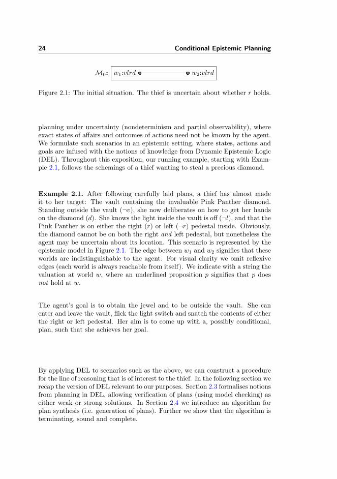
M0: w1:vlrd w2:vlrd

Figure 2.1: The initial situation. The thief is uncertain about whether r holds.

planning under uncertainty (nondeterminism and partial observability), whereexact states of affairs and outcomes of actions need not be known by the agent.We formulate such scenarios in an epistemic setting, where states, actions andgoals are infused with the notions of knowledge from Dynamic Epistemic Logic(DEL). Throughout this exposition, our running example, starting with Exam-ple 2.1, follows the schemings of a thief wanting to steal a precious diamond.

Example 2.1. After following carefully laid plans, a thief has almost madeit to her target: The vault containing the invaluable Pink Panther diamond.Standing outside the vault (¬v), she now deliberates on how to get her handson the diamond (d). She knows the light inside the vault is off (¬l), and that thePink Panther is on either the right (r) or left (¬r) pedestal inside. Obviously,the diamond cannot be on both the right and left pedestal, but nonetheless theagent may be uncertain about its location. This scenario is represented by theepistemic model in Figure 2.1. The edge between w1 and w2 signifies that theseworlds are indistinguishable to the agent. For visual clarity we omit reflexiveedges (each world is always reachable from itself). We indicate with a string thevaluation at world w, where an underlined proposition p signifies that p doesnot hold at w.

The agent’s goal is to obtain the jewel and to be outside the vault. She canenter and leave the vault, flick the light switch and snatch the contents of eitherthe right or left pedestal. Her aim is to come up with a, possibly conditional,plan, such that she achieves her goal.

By applying DEL to scenarios such as the above, we can construct a procedurefor the line of reasoning that is of interest to the thief. In the following section werecap the version of DEL relevant to our purposes. Section 2.3 formalises notionsfrom planning in DEL, allowing verification of plans (using model checking) aseither weak or strong solutions. In Section 2.4 we introduce an algorithm forplan synthesis (i.e. generation of plans). Further we show that the algorithm isterminating, sound and complete.

2.2 Dynamic Epistemic Logic 25

2.2 Dynamic Epistemic Logic

Dynamic epistemic logics describe knowledge and how actions change it. Thesechanges may be epistemic (changing knowledge), ontic (changing facts) or both.The work in this paper deals only with the single-agent setting, though webriefly discuss the multi-agent setting in Section 2.5. As in Example 2.1, agentknowledge is captured by epistemic models. Changes are encoded using eventmodels (defined below). The following concise summary of DEL is meant as areference for the already familiar reader. The unfamiliar reader may consult [vanDitmarsch and Kooi, 2008, Ditmarsch et al., 2007] for a thorough treatment.

Definition 2.2 (Epistemic Language). Let a set of propositional symbols P begiven. The language LDEL(P ) is given by the following BNF:

φ ::= > | p | ¬φ | φ ∧ φ | Kφ | [E , e]φ

where p ∈ P , E denotes an event model on LDEL(P ) as (simultaneously) definedbelow, and e ∈ D(E). K is the epistemic modality and [E , e] the dynamicmodality. We use the usual abbreviations for the other boolean connectives, aswell as for the dual dynamic modality 〈E , e〉φ := ¬ [E , e]¬φ. The dual of K isdenoted K̃. Kφ reads as "the (planning) agent knows φ" and [E , e]φ as "afterall possible executions of (E , e), φ holds".

Definition 2.3 (Epistemic Models). An epistemic model on LDEL(P ) is a tupleM = (W,∼, V ), where W is a set of worlds, ∼ is an equivalence relation (theepistemic relation) on W , and V : P → 2W is a valuation. D(M) = W denotesthe domain ofM. For w ∈W we name (M, w) a pointed epistemic model, andrefer to w as the actual world of (M, w).

To reason about the dynamics of a changing system, we make use of eventmodels. The formulation of event models we use in this paper is due to vanDitmarsch and Kooi [van Ditmarsch and Kooi, 2008]. It adds ontic change tothe original formulation of [Baltag et al., 1998] by adding postconditions toevents.

Definition 2.4 (Event Models). An event model on LDEL(P ) is a tuple E =(E,∼, pre, post), where

– E is a set of (basic) events,– ∼⊆ E × E is an equivalence relation called the epistemic relation,– pre : E → LDEL(P ) assigns to each event a precondition,– post : E → (P → LDEL(P )) assigns to each event a postcondition.

26 Conditional Epistemic Planning

D(E) = E denotes the domain of E . For e ∈ E we name (E , e) a pointed eventmodel, and refer to e as the actual event of (E , e).

Definition 2.5 (Product Update). LetM = (W,∼, V ) and E = (E,∼′, pre, post)be an epistemic model resp. event model on LDEL(P ). The product update ofM with E is the epistemic model denotedM⊗E = (W ′,∼′′, V ′), where

– W ′ = {(w, e) ∈W × E | M, w |= pre(e)},– ∼′′= {((w, e), (v, f)) ∈W ′ ×W ′ | w ∼ v and e ∼′ f},– V ′(p) = {(w, e) ∈W ′ | M, w |= post(e)(p)} for each p ∈ P .

Definition 2.6 (Satisfaction Relation). Let a pointed epistemic model (M, w)on LDEL(P ) be given. The satisfaction relation is given by the usual semantics,where we only recall the definition of the dynamic modality:

M, w |= [E , e]φ iffM, w |= pre(e) impliesM⊗E , (w, e) |= φ

where φ ∈ LDEL(P ) and (E , e) is a pointed event model. We write M |= φto mean M, w |= φ for all w ∈ D(M). Satisfaction of the dynamic modalityfor non-pointed event models E is introduced by abbreviation, viz. [E ]φ :=∧e∈D(E) [E , e]φ. Furthermore, 〈E〉φ := ¬ [E ]¬φ.1

Throughout the rest of this paper, all languages (sets of propositional symbols)and all models (sets of possible worlds) considered are implicitly assumed to befinite.

2.3 Conditional Plans in DEL

One way to sum up automated planning is that it deals with the reasoningside of acting [Ghallab et al., 2004]. When planning under uncertainty, actionscan be nondeterministic and the states of affairs partially observable. In thefollowing, we present a formalism expressing planning under uncertainty in DEL,while staying true to the notions of automated planning. We consider a systemsimilar to that of [Ghallab et al., 2004, sect. 17.4], which motivates the followingexposition. The type of planning detailed here is offline, where planning isdone before acting. All reasoning must therefore be based on the agent’s initialknowledge.

1Hence, M, w |= 〈E〉φ ⇔ M, w |= ¬ [E]¬φ ⇔ M, w |= ¬(∧

e∈D(E) [E, e]¬φ) ⇔ M, w |=∨e∈D(E) ¬ [E, e]¬φ⇔M, w |=

∨e∈D(E) 〈E, e〉φ.

2.3 Conditional Plans in DEL 27

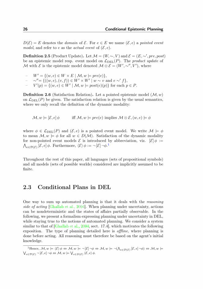
M′: u1:vlrd u2:vlrd

Figure 2.2: A model consisting of two information cells

2.3.1 States and Actions: The Internal Perspective

Automated planning is concerned with achieving a certain goal state from agiven initial state through some combination of available actions. In our case,states are epistemic models. These models represent situations from the perspec-tive of the planning agent. We call this the internal perspective—the modelleris modelling itself. The internal perspective is discussed thoroughly in [Aucher,2010, Bolander and Andersen, 2011].

Generally, an agent using epistemic models to model its own knowledge andignorance, will not be able to point out the actual world. Consider the epistemicmodel M0 in Figure 2.1, containing two indistinguishable worlds w1 and w2.Regarding this model to be the planning agent’s own representation of the initialstate of affairs, the agent is of course not able to point out the actual world. Itis thus natural to represent this situation as a non-pointed epistemic model. Ingeneral, when the planning agent wants to model a future (imagined) state ofaffairs, she does so by a non-pointed model.

The equivalence classes (wrt. ∼) of a non-pointed epistemic model are calledthe information cells of that model (in line with the corresponding concept in[Baltag and Smets, 2008]). We generally identify any equivalence class [w]∼ of amodelM with the submodel it induces, that is, we identify [w]∼ withM � [w]∼.We also use the expression information cell on LDEL(P ) to denote any connectedepistemic model on LDEL(P ), that is, any epistemic model consisting of a singleinformation cell. All worlds in an information cell satisfy the same K-formulas(formulas of the formKφ), thus representing the same situation as seen from theagent’s internal perspective. Each information cell of a (non-pointed) epistemicmodel represents a possible state of knowledge of the agent.

Example 2.7. Recall that our jewel thief is at the planning stage, with herinitial information cellM0. She realises that entering the vault and turning onthe light will reveal the location of the Pink Panther. Before actually perform-ing these actions, she can rightly reason that they will lead her to know thelocation of the diamond, though whether that location is left or right cannot bedetermined (yet).

Her representation of the possible outcomes of going into the vault and turningon the light is the model M′ in Figure 2.2. The information cells M′ � {u1}

28 Conditional Epistemic Planning

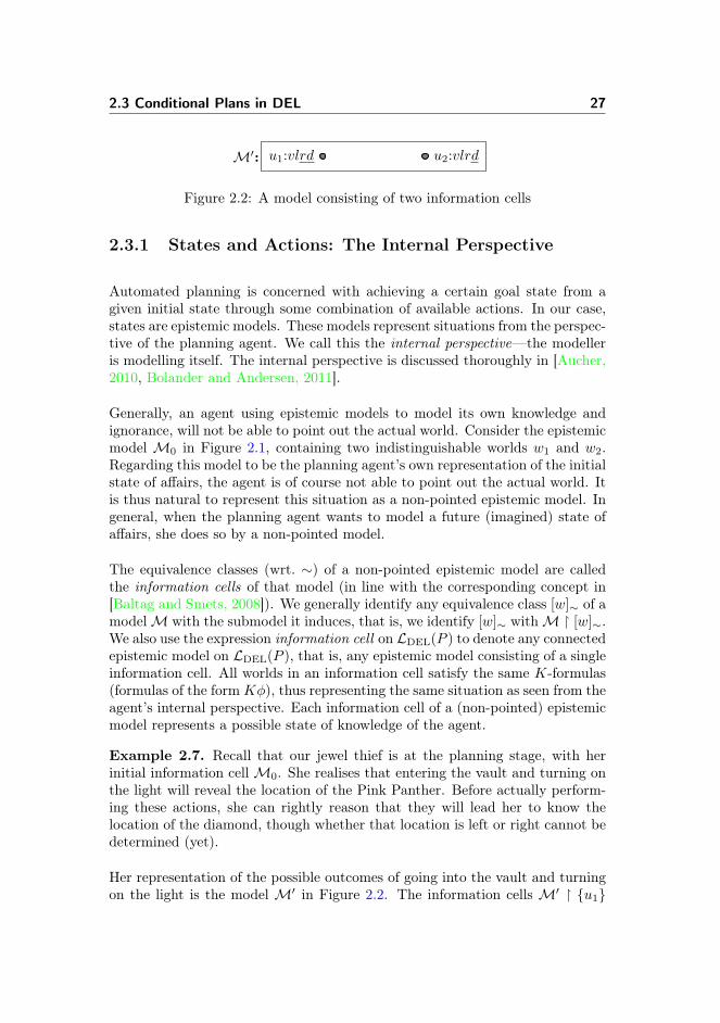
g:〈v ∧ ¬d, {d 7→ ¬r}〉

take_left

h:〈v ∧ ¬d, {d 7→ r}〉

take_right

e1:〈r ∧ v, {l 7→ >}〉

e2:〈¬r ∧ v, {l 7→ >}〉flick

f1:〈v ∨ (¬v ∧ ¬l) , {v 7→ ¬v}〉 f2:〈¬v ∧ l ∧ r, {v 7→ ¬v}〉 f3:〈¬v ∧ l ∧ ¬r, {v 7→ ¬v}〉

move

Figure 2.3: Event models representing the actions of the thief

and M′ � {u2} of M′ are exactly the two distinguishable states of knowledgethe jewel thief considers possible prior turning the light on in the vault.

In the DEL framework, actions are naturally represented as event models. Dueto the internal perspective, these are also taken to be non-pointed. For instance,in a coin toss action, the agent cannot beforehand point out which side will landface up.

Example 2.8. Continuing Example 2.7 we now formalize the actions availableto our thieving agent as the event models in Figure 2.3. We use the sameconventions for edges as we did for epistemic models. For a basic event e welabel it 〈pre(e), post(e)〉.2

The agent is endowed with four actions: take_left, resp. take_right, representtrying to take the diamond from the left, resp. right, pedestal; the diamondis obtained only if it is on the chosen pedestal. Both actions require the agentto be inside the vault and not holding the diamond. flick requires the agent tobe inside the vault and turns the light on. Further, it reveals which pedestalthe diamond is on. move represents the agent moving in or out of the vault,revealing the location of the diamond provided the light is on.

It can be seen that the epistemic modelM′ in Example 2.7 is the result of twosuccessive product updates, namelyM0 ⊗move⊗ flick.

2.3.2 Applicability, Plans and Solutions

Reasoning about actions from the initial state as in Example 2.8 is exactlywhat planning is all about. We have however omitted an important component

2For a proposition p whose truth value does not change in e we assume the identity mappingpost(e)(p) = p, as is also the convention in automated planning.

2.3 Conditional Plans in DEL 29

in the reasoning process, one which is crucial. The notion of applicability inautomated planning dictates when the outcomes of an action are defined. Theidea translates to DEL by insisting that no world the planning agent considerspossible is eliminated by the product update of an epistemic model with anevent model.

Definition 2.9 (Applicability). An event model E is said to be applicable inan epistemic modelM ifM |= 〈E〉>.

This concept of applicability is easily shown to be equivalent with the one definedin [Bolander and Andersen, 2011] when restricting the latter to the single-agentcase. However, for our purposes of describing plans as formulas, we need toexpress applicability as formulas as well. The discussion in [de Lima, 2007, sect.6.6] also notes this aspect, insisting that actions must be meaningful. The samesentiment is expressed by our notion of applicability.

The situation in Example 2.7 calls for a way to express conditional plans.Clearly, our agent can only snatch the jewel from the correct pedestal condi-tioned on how events unfold when she acts. To this end we introduce a languagefor conditional plans allowing us to handle such contingencies.

Definition 2.10 (Plan Language). Given a finite set A of event models onLDEL(P ), the plan language LP(P,A) is given by:

π ::= E | skip | if Kφ then π else π | π;π

where E ∈ A and φ ∈ LDEL(P ). We name members π of this language plans,and use if Kφ then π as shorthand for if Kφ then π else skip.

The reading of the plan constructs are "do E", "do nothing", "if Kφ then π, elseπ′", and "first π then π′" respectively. Note that the condition of the if-then-elseconstruct is required to be a K-formula. This is to ensure that the planningagent can only make her choices of actions depend on worlds that are distin-guishable to her (cf. the discussion of the internal perspective in Section 2.3.1).The idea is similar to the meaningful plans of [de Lima, 2007], where branchingis only allowed on epistemically interpretable formulas.

An alternative way of specifying conditional plans is policies, where (in our ter-minology) each information cell maps to an event model [Ghallab et al., 2004,Sect. 16.2]. There are slight differences between the expressiveness of condi-tional plans and policies (e.g. policies can finitely represent repetitions); ourmain motivation for not using policies is that it would require an enumerationof each information cell of the planning domain.

30 Conditional Epistemic Planning

Definition 2.11 (Translation). We define a strong translation J·Ks · and a weaktranslation J·Kw · as functions from LP(P,A)× LDEL(P ) into LDEL(P ) by:

JEKs φ := 〈E〉> ∧ [E ]Kφ

JEKw φ := 〈E〉> ∧ K̃ 〈E〉KφJskipK· φ := φJif φ′ then π else π′K· φ := (φ′ → JπK· φ) ∧ (¬φ′ → Jπ′K· φ)Jπ;π′K· φ := JπK· (Jπ

′K· φ)

Plans describe the manner in which actions are carried out. We interpret plansπ relative to a formula φ and want to answer the question of whether or notπ achieves φ. Using Definition 2.11 we can answer this question by verifyingtruth of the DEL formula provided by the translations. This is supported by theresults of Section 2.4. We concisely read JπKs φ as "π achieves φ", and JπKw φ as"π may achieve φ" (elaborated below). By not specifying separate semantics forplans our framework is kept as simple as possible. Note that applicability (Def-inition 2.9) is built into the translations through the occurrence of the conjunct〈E〉> in both the strong translation JEKs φ and the weak translation JEKw φ.

The difference between the two translations relate to the robustness of plans:JπKs φ, resp. JπKw φ, means that every step of π is applicable and that followingπ always leads, resp. may lead, to a situation where φ is known.

Definition 2.12 (Planning Problems and Solutions). Let P be a finite set ofpropositional symbols. A planning problem on P is a triple P = (M0,A, φg)where

– M0 is an information cell on LDEL(P ) called the initial state.– A is a finite set of event models on LDEL(P ) called the action library.– φg ∈ LDEL(P ) is the goal (formula).

We say that a plan π ∈ LP(P,A) is a strong solution to P if M0 |= JπKs φg, aweak solution ifM0 |= JπKw φg and not a solution otherwise.

Planning problems are defined with the sentiment we’ve propagated in our ex-amples up until now. The agent is presently inM0 and wishes φg to be the case.To this end, she reasons about the actions (event models) in her action libraryA, creating a conditional plan. Using model checking, she can verify whetherthis plan is either a weak or strong solution, since plans translate into formulasof LDEL(P ). Further, [van Ditmarsch and Kooi, 2008] gives reduction axiomsfor DEL-formulas, showing that any formula containing the dynamic modalitycan be expressed as a formula in (basic) epistemic logic. Consequently, planverification can be seen simply as epistemic reasoning aboutM0.

2.4 Plan Synthesis 31

Example 2.13. We continue our running example by discussing it formally asa planning problem and considering the solutions it allows. The initial stateis still M0, and the action library A = {flick,move, take_left, take_right}. Wediscuss the plans below and their merit for our thief.

– π1 = flick;move; if Kr then take_right else take_left;move– π2 = move; take_right;move– π3 = move; flick; take_right;move– π4 = move; flick; if Kr then take_right else take_left;move

We consider two planning problems varying only on the goal formula, P1 =(M0,A, d ∧ ¬v) and P2 = (M0,A, K̃d ∧ ¬v). In P1 her goal is to obtain thediamond and be outside the vault, whereas in P2 she wishes to be outside thevault possibly having obtained the diamond.

Let π′1 = move; if Kr then take_right else take_left;move and note that π1 =flick;π′1. Using the strong translation of π1, we get M0 |= Jπ1Ks φg iff M0 |=〈flick〉> ∧ [flick] Jπ′1Ks φg. AsM0 |= 〈flick〉> does not hold, π1 is not a solution.This is expected, since flicking the switch in the initial state is not an applicableaction. Verifying that π2 is a strong solution to P2 amounts to checking ifM0 |= Jπ2Ks K̃d ∧ ¬v which translates to

M0 |= 〈move〉> ∧

[move]K(〈take_right〉> ∧ [take_right]K

(〈move〉> ∧ [move]K

(K̃d ∧ ¬v

)))With the same approach we can conclude that π2 is not a solution to P1, π3 isa weak solution to P1 and P2, and π4 is a strong solution to P1 and P2.

2.4 Plan Synthesis

We now show how to synthesise conditional plans for solving planning prob-lems. To synthesise plans, we need a mechanism for coming up with formulascharacterising information cells for if-then-else constructs to branch on. Inspiredby [Barwise and Moss, 1996, van Benthem, 1998], these are developed in thefollowing. Proofs are omitted, as they are straightforward and similar to proofsin the aforementioned references.

Definition 2.14 (Characterising Formulas). Let M = (W,∼, V ) denote aninformation cell on LDEL(P ). We define for all w ∈ W a formula φw by: φw =∧p∈V (w) p ∧

∧p∈P−V (w) ¬p. We define the characterising formula for M, δM,

as follows: δM = K(∧w∈W K̃φw ∧K

∨w∈W φw).

32 Conditional Epistemic Planning

Lemma 2.15. Let M be an information cell on LDEL(P ). Then for all epis-temic models M′ = (W ′,∼′, V ′) and all w′ ∈ W ′ we have that (M′, w′) |= δMif and only if there exists a w ∈ D(M) such that (M, w) - (M′, w′).3

For purposes of synthesis, we use the product update solely on non-pointedepistemic and event models. Lemma 2.16 shows that satisfaction of the dynamicmodality for non-pointed event models in non-pointed epistemic models relatesto the product update in the obvious way.

Lemma 2.16. Let M be an epistemic model and E an event model. ThenM |= [E ]φ iffM⊗E |= φ.

Proof. M |= [E ]φ ⇔ for all w ∈ D(M) :M, w |= [E ]φ ⇔for all w ∈ D(M) :M, w |=

∧e∈D(E)[E , e]φ ⇔

for all (w, e) ∈ D(M)×D(E) :M, w |= [E , e]φ ⇔for all (w, e) ∈ D(M)×D(E) :M, w |= pre(e) impliesM⊗E , (w, e) |= φ ⇔for all (w, e) ∈ D(M⊗E) :M⊗E , (w, e) |= φ ⇔ M⊗ E |= φ.

2.4.1 Planning Trees

When synthesising plans, we explicitly construct the search space of the problemas a labelled and-or tree, a familiar model for planning under uncertainty[Ghallab et al., 2004]. Our and-or trees are called planning trees.

Definition 2.17. A planning tree is a finite, labelled and-or tree in which eachnode n is labelled by an epistemic model M(n), and each edge (n,m) leavingan or-node is labelled by an event model E(n,m).

Planning trees for planning problems P = (M0,A, φg) are constructed as fol-lows. Let the initial planning tree T0 consist of just one or-node root(T0) withM(root(T0)) =M0 (the root labels the initial state). A planning tree for P isthen any tree that can be constructed from T0 by repeated applications of thefollowing non-deterministic tree expansion rule.

Definition 2.18 (Tree Expansion Rule). Let T be a planning tree for a planningproblem P = (M0,A, φg). The tree expansion rule is defined as follows. Pick anor-node n in T and an event model E ∈ A applicable inM(n) with the provisothat E does not label any existing outgoing edges from n. Then:

3Here (M, w) - (M′, w) denotes that (M, w) and (M′, w) are bisimilar according to thestandard notion of bisimulation on pointed epistemic models.

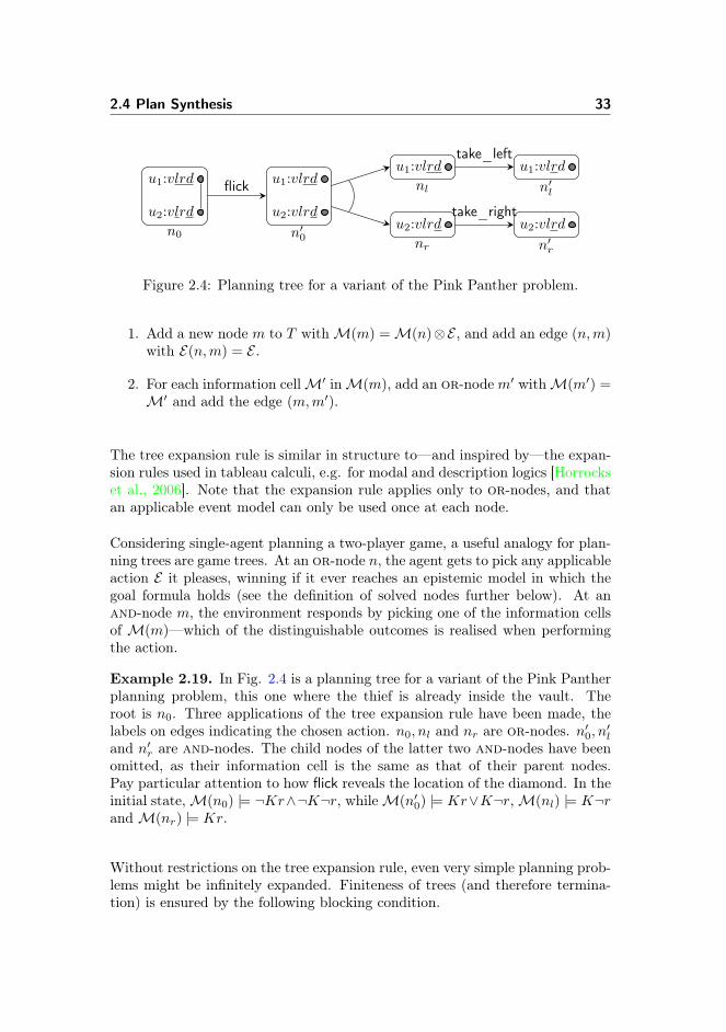
2.4 Plan Synthesis 33

u1:vlrd

u2:vlrdn0

u1:vlrd

u2:vlrdn′0

u1:vlrdnl

u2:vlrdnr

u1:vlrdn′l

u2:vlrdn′r

flick

take_left

take_right

Figure 2.4: Planning tree for a variant of the Pink Panther problem.

1. Add a new node m to T withM(m) =M(n)⊗E , and add an edge (n,m)with E(n,m) = E .

2. For each information cellM′ inM(m), add an or-nodem′ withM(m′) =M′ and add the edge (m,m′).

The tree expansion rule is similar in structure to—and inspired by—the expan-sion rules used in tableau calculi, e.g. for modal and description logics [Horrockset al., 2006]. Note that the expansion rule applies only to or-nodes, and thatan applicable event model can only be used once at each node.

Considering single-agent planning a two-player game, a useful analogy for plan-ning trees are game trees. At an or-node n, the agent gets to pick any applicableaction E it pleases, winning if it ever reaches an epistemic model in which thegoal formula holds (see the definition of solved nodes further below). At anand-node m, the environment responds by picking one of the information cellsof M(m)—which of the distinguishable outcomes is realised when performingthe action.

Example 2.19. In Fig. 2.4 is a planning tree for a variant of the Pink Pantherplanning problem, this one where the thief is already inside the vault. Theroot is n0. Three applications of the tree expansion rule have been made, thelabels on edges indicating the chosen action. n0, nl and nr are or-nodes. n′0, n′land n′r are and-nodes. The child nodes of the latter two and-nodes have beenomitted, as their information cell is the same as that of their parent nodes.Pay particular attention to how flick reveals the location of the diamond. In theinitial state,M(n0) |= ¬Kr∧¬K¬r, whileM(n′0) |= Kr∨K¬r,M(nl) |= K¬randM(nr) |= Kr.

Without restrictions on the tree expansion rule, even very simple planning prob-lems might be infinitely expanded. Finiteness of trees (and therefore termina-tion) is ensured by the following blocking condition.

34 Conditional Epistemic Planning

B1 The tree expansion rule may not be applied to a node n for which thereexists an ancestor node m withM(m) -M(n).4

A planning tree for a planning problem P is called B1-saturated if no moreexpansions are possible satisfying condition B1.

Lemma 2.20 (Termination). Any procedure that builds a B1-saturated planningtree for a planning problem P by repeated application of the tree expansion ruleterminates.

Proof. Planning trees built by repeated application of the tree expansion ruleare finitely branching: the action library is finite, and every epistemic model hasonly finitely many information cells. Furthermore, condition B1 ensures that nobranch has infinite length: there only exists finitely many mutually non-bisimilarepistemic models over any given finite set of propositional symbols [Bolanderand Andersen, 2011]. König’s Lemma now implies finiteness of the planningtree.

Definition 2.21 (Solved Nodes). Let T be any (not necessarily saturated)planning tree for a planning problem P = (M0,A, φg). By recursive definition,a node n in T is called solved if one of the following holds:

• M(n) |= φg (the node satisfies the goal formula).• n is an or-node having at least one solved child.• n is an and-node having all its children solved.

Continuing the game tree analogy, we see that a solved node corresponds toone for which there exists a winning strategy. Regardless of the environment’schoice, the agent can achieve its goal. Let T and P be as above. Below we showthat when a node n is solved, it is possible to construct a (strong) solution tothe planning problem (M(n),A, φg). In particular, if the root node is solved, astrong solution to P can be constructed. As it is never necessary to expand asolved node, nor any of its descendants, we can augment the blocking conditionB1 in the following way.

B2 The tree expansion rule may not be applied to a node n if one of the followingholds: 1) n is solved; 2) n has a solved ancestor; 3) n has an ancestor nodem withM(m) -M(n).

4HereM(m) -M(n) denotes thatM(m) andM(n) are bisimilar according to the stan-dard notion of bisimulation between non-pointed epistemic models.

2.4 Plan Synthesis 35

In the following, we will assume that all planning trees have been built accordingto B2. One consequence is that a solved or-node has exactly one solved child.We make use of this in the following definition.

Definition 2.22 (Plans for Solved Nodes). Let T be any planning tree forP = (M0,A, φg). For each solved node n in T , a plan π(n) is defined recursivelyby:• ifM(n) |= φg, then π(n) = skip.• if n is an or-node and m its solved child, then π(n) = E(n,m);π(m).• if n is an and-node with children m1, . . . ,mk, then π(n) =

if δM(m1) then π(m1) else if δM(m2) then π(m2) else · · · if δM(mk) then π(mk)

Example 2.23. For the goal of achieving the diamond, φg = d, we have thatthe root n0 of the planning tree of Figure 2.4 is solved, as both n′l and n

′r satisfy

the goal formula. Definition 2.22 gives us

π(n0) = flick; if δM(nl) then take_left; skip else if δM(nr)then take_right; skip

This plan can easily be shown to be a strong solution to the planning problemof achieving d from the initial stateM(n0). In our soundness result below, weshow that plans of solved roots are always strong solutions to their correspondingplaning problems.

Theorem 2.24 (Soundness). Let T be a planning tree for a problem P suchthat root(T ) is solved. Then π(root(T )) is a strong solution to P.

Proof. We need to prove that π(root(T )) is a strong solution to P, that is,M0 |= Jπ(root(T ))Ks φg. SinceM0 is the label of the root, this can be restated asM(root(T )) |= Jπ(root(T ))Ks φg. To prove this fact, we will prove the followingstronger claim:

• For each solved node n in T ,M(n) |= Jπ(n)Ks φg.

We prove this by induction on the height of n. The base case is when n is a leaf.Since n is solved, we must have M(n) |= φg. In this case π(n) = skip. FromM(n) |= φg we can conclude M(n) |= JskipKs φg, that is, M(n) |= Jπ(n)Ks φg.This covers the base case. For the induction step, assume that for all solvednodes m of height < h,M(m) |= Jπ(m)Ks φg. Let n be an arbitrary solved noden of height h. We then need to show M(n) |= Jπ(n)Ks φg. We have two casesto consider, depending on whether n is an and- or an or-node.

Case 1: n is an and-node. Let m1, . . . ,mk be the children of n. By definition,all of these are solved. We have π(n) = if δM(m1) then π(m1) else if δM(m2) then

36 Conditional Epistemic Planning

π(m2) else · · · if δM(mk) then π(mk) else skip. The induction hypothesis givesusM(mi) |= Jπ(mi)Ks φg for all i = 1, . . . , k.

Claim 1. M(n) |= δM(mi) → Jπ(mi)Ks φg, for all i = 1, . . . , k.

Proof of claim. Let w ∈ D(M(n)) be chosen arbitrarily. We then need to provethat ifM(n), w |= δM(mi) thenM(n), w |= Jπ(mi)Ks φg. AssumingM(n), w |=δM(mi), we get from Lemma 2.15 that there must be a w′ ∈ D(M(mi)) suchthatM(mi), w

′ -M(n), w. SinceM(mi) |= Jπ(mi)Ks φg, in particular we getM(mi), w

′ |= Jπ(mi)Ks φg, and thusM(n), w |= Jπ(mi)Ks φg.

Claim 2. M(n) |=∨

i=1,...,k

δM(mi).

Proof of claim. Let w ∈ D(M(n)) be chosen arbitrarily. We then need to provethat M(n), w |= ∨i=1,...,kδM(mi). Since w ∈ D(M(n)) it must belong to oneof the information cells of M(n), that is, w ∈ D(M(mj)) for some j. ThusM(n), w -M(mj), w. From Lemma 2.15 we then getM(n), w |= δM(mj), andthusM(n), w |= ∨i=1,...,kδM(mi).

From (1) and (2), we now get:

M(n) |=∧

i=1,...,k

(δM(mi) → Jπ(mi)Ks φg) ∧∨

i=1,...,k

δM(mi) ⇒

M(n) |=∧

i=1,...,k

(δM(mi) ∧

∧j=1,...,i−1

¬δM(mj) → Jπ(mi)Ks φg

)∧( ∧i=1,...,k

¬δM(mi) → JskipKs φg

)⇒

M(n) |= (δM(m1) → Jπ(m1)Ks φg) ∧ (¬δM(m1) →(δM(m2) → Jπ(m2)Ks φg) ∧ (¬δM(m2) →· · ·(δM(mk) → Jπ(mk)Ks φg) ∧ (¬δM(mk) →

JskipKs φg) · · · )⇒M(n) |= Jif δM(m1) then π(m1) else

if δM(m2) then π(m2) else

· · ·if δM(mk) then π(mk) else

skipK φg ⇒M(n) |= Jπ(n)Ks φg.

Case 2: n is an or-node. Here we have π(n) = E(n,m);π(m) for the solvedchild m of n. The induction hypothesis gives M(m) |= Jπ(m)Ks φg, and henceM(m) |= K Jπ(m)Ks φg. We now showM(n) |= Jπ(n)Ks φg. Since, by definition,M(m) =M(n)⊗E(n,m), we getM(n)⊗E(n,m) |= K Jπ(m)Ks φg. We can now

2.4 Plan Synthesis 37

apply Lemma 2.16 to concludeM(n) |= [E(n,m)]K Jπ(m)Ks φg. By definition,E(n,m) must be applicable inM(n), that is,M(n) |= 〈E(n,m)〉>. Thus we nowhave M(n) |= 〈E(n,m)〉> ∧ [E(n,m)]K Jπ(m)Ks φg. Using Definition 2.11, wecan rewrite this asM(n) |= JE(n,m)Ks Jπ(m)Ks φg. Using Definition 2.11 again,we get M(n) |= JE(n,m);π(m)Ks φg, and thus finally M(n) |= Jπ(n)Ks φg, asrequired.

Theorem 2.25 (Completeness). If there is a strong solution to the planningproblem P = (M0,A, φg), then a planning tree T for P can be constructed, suchthat root(T ) is solved.

Proof. We first prove the following claim.

Claim 1. If (if φ then π1 else π2) is a strong solution to P = (M0,A, φg), thenso is π1 or π2.

Proof of claim. Assume (if φ then π1 else π2) is a strong solution to (M0,A, φg),that is, M0 |= Jif φ then π1 else π2Ks φg. Then, by definition, M0 |= (φ →Jπ1Ks φg) ∧ (¬φ → Jπ2Ks φg). Since M0 is an information cell, and φ is a K-formula, we must have either M0 |= φ or M0 |= ¬φ. Thus we get that eitherM0 |= Jπ1Ks φg orM0 |= Jπ2Ks φg, as required.

Note that we have Jskip;πKs φg = JskipKs (JπKs φg) = JπKs φg. Thus, we canwithout loss of generality assume that no plan contains a subexpression of theform skip;π. The length of a plan π, denoted |π|, is defined recursively by:|skip| = 1; |E| = 1; |if φ then π1 else π2| = |π1|+ |π2|; |π1;π2| = |π1|+ |π2|.

Claim 2. Let π be a strong solution to P = (M0,A, φg) with |π| ≥ 2. Thenthere exists a strong solution of the form E ;π′ with |E ;π′| ≤ |π|.

Proof of claim. Proof by induction on |π|. The base case is |π| = 2. We havetwo cases, π = if φ then π1 else π2 and π = π1;π2, both with |π1| = |π2| = 1.If π is the latter, it already has desired the form. If π = if φ then π1 else π2

we have by Claim 1 that either π1 or π2 is a strong solution to P. Thus alsoeither π1; skip or π2; skip is a strong solution to P, and both of these havelength |π|. This completes the base case. For the induction step, we assumethat if π′, with |π′| < l, is a strong solution to a planning problem P ′, thenthere exists is a strong solution of the form (E ;π′′), with |E ;π′′| ≤ |π′|. Nowconsider a plan π of length l which is a strong solution to P. We again havetwo cases to consider, π = if φ then π1 else π2 and π = π1;π2. If π = π1;π2

is a strong solution to P, then π1 is a strong solution to the planning problemP ′ = (M0,A, Jπ2Ks φg), asM0 |= Jπ1;π2Ks φg ⇔M0 |= Jπ1Ks Jπ2Ks φg. Clearly|π1| < l, so the induction hypothesis gives that there is a strong solution (E ;π′1)

38 Conditional Epistemic Planning

to P ′, with |E ;π′1| ≤ |π1|. Then, E ;π′1;π2 is a strong solution to P and we have|E ;π′1;π2| = |E ;π′1| + |π2| ≤ |π1| + |π2| = |π|. If π = if φ then π1 else π2 is astrong solution to P, then we have by Claim 1 that either π1 or π2 is a strongsolution to P. With both |π1| < l and |π2| < l, the induction hypothesis givesthe existence a strong solution E ;π′, with |E ;π′| ≤ |π|. This completes the proofof the claim.

We now prove the theorem by induction on |π|, where π is a strong solutionto P = (M0,A, φg). We need to prove that there exists a planning tree Tfor P in which the root is solved. Let T0 denote the planning tree for P onlyconsisting of its root node with labelM0. The base case is when |π| = 1. Here,we have two cases, π = skip and π = E . In the first case, the planning treeT0 already has its root solved, since M0 |= JskipKs φg ⇔ M0 |= φg. In thesecond case π = E . Since π is a strong solution to P, we have M0 |= JEKs φg,that is, M0 |= 〈E〉> ∧ [E ]Kφg. Thus E is applicable in M0 meaning that wecan apply the tree expansion rule to T0, which will produce an and-node mwith E(root(T0),m) = E and M(m) = M0 ⊗ E . Call the expanded tree T1.Since we have M0 |= [E ]Kφg, Lemma 2.16 gives us M0 ⊗ E |= Kφg, that is,M(m) |= Kφg, and hence M(m) |= φg. This implies that M(m) and thusroot(T1) is solved. The base case is hereby completed.

For the induction step, assume that a planning tree with solved root can beconstructed for problems with strong solutions of length < l. Let π be a strongsolution to P with |π| = l. By Claim 2, there exists a strong solution of the formE ;π′ with |E ;π′| ≤ |π|. As M0 |= JE ;π′Ks φg ⇔ M0 |= JEKs Jπ′Ks φg ⇔ M0 |=〈E〉> ∧ [E ]K(Jπ′Ks φg), the tree expansion rule can be applied by picking E andM0. This produces the and-node m with E(n,m) = E andM(m) =M0 ⊗ E .m1, . . . ,mk are the children of m, and M(mi) = Mi the information cellsin M(m). From M0 |= [E ]K(Jπ′Ks φg) we get M0 ⊗ E |= K Jπ′Ks φg, usingLemma 2.16. This impliesMi |= K Jπ′Ks φg, and henceMi |= Jπ′Ks φg, for eachinformation cell Mi of M(m) = M0 ⊗ E . Thus π′ must be a strong solutionto each of the planning problems Pi = (Mi,A, φg). As |π′| < |E ;π′| ≤ l,the induction hypothesis gives that planning trees Ti with solved roots can beconstructed for each Pi. Let T denote T0 expanded with m,m1, . . . ,mk, andeach Ti be the subtree rooted at mi. Then each of the nodes mi are solved inT , and in turn both m and root(T ) are solved.

2.4.2 Strong Planning Algorithm

With all the previous in place, we now have an algorithm for synthesising strongsolutions for planning problems P, given as follows.

2.4 Plan Synthesis 39

StrongPlan(P)1 Let T be the plan. tree only consisting of root(T ) labelled by the init. state of P.2 Repeatedly apply the tree expansion rule of P to T until it is B2-saturated.3 If root(T ) is solved, return π(root(T )), otherwise return fail.

Theorem 2.26. StrongPlan(P) is a terminating, sound and complete algo-rithm for producing strong solutions to planning problems. Soundness meansthat if StrongPlan(P) returns a plan, it is a strong solution to P. Com-pleteness means that if P has a strong solution, StrongPlan(P) will returnone.

Proof. Termination comes from Lemma 2.20 (with B1 replaced by the strongercondition B2), soundness from Theorem 2.24 and completeness from Theorem2.25 (given any two saturated planning trees T1 and T2 for the same planningproblem, the root node of T1 is solved iff the root node of T2 is).

2.4.3 Weak Planning Algorithm

With few changes, the machinery already in place gives an algorithm for syn-thesising weak solutions. Rather than requiring all children of an and-node besolved, we require only one. This corresponds to the notion of weak, defined inDefinition 2.11. Only one possible execution need lead to the goal.

Definition 2.27 (Weakly Solved Nodes). A node n is called weakly solved ifeitherM(n) |= φg or n has at least one weakly solved child.

We keep the tree expansion rule, but make use of a new blocking condition B3

using Definition 2.27 rather than Definition 2.21.

Definition 2.28 (Plans for Weakly Solved Nodes). Let T be any planning treefor P = (M0,A, φg). For each weakly solved node n in T , a plan πw(n) isdefined recursively by:

• ifM(n) |= φg, then πw(n) = skip

• if n is an or-node andm its weakly solved child, then πw(n) = E(n,m);πw(m)

• if n is an and-node and m its weakly solved child, then πw(n) = πw(m)

The algorithm for weak planning is defined as follows.

40 Conditional Epistemic Planning

WeakPlan(P)1 Let T be the plan. tree only consisting of root(T ) labelled by the init. state of P.2 Repeatedly apply the tree expansion rule of P to T until it is B3-saturated.3 If root(T ) is weakly solved, return πw(root(T )), otherwise return fail.

Theorem 2.29. WeakPlan(P) is a terminating, sound and complete algo-rithm for producing weak solutions to planning problems.

2.5 Related and Future Work

In this paper, we have presented a syntactic characterisation of weak and strongsolutions to epistemic planning problems, that is, we have characterised solutionsas formulas. [Bolander and Andersen, 2011] takes a semantic approach to strongsolutions for epistemic planning problems. In their work plans are sequences ofactions, requiring conditional choice of actions at different states to be encodedin the action structure itself. We represent choice explicitly, using a languageof conditional plans. An alternative to our approach of translating conditionalplans into formulas of DEL would be to translate plans directly into (complex)event models. This is the approach taken in [Baltag and Moss, 2004], where theyhave a language of epistemic programs similar to our language of plans (modulothe omission of ontic actions). Using this approach in a planning setting, onecould translate each possible plan π into the corresponding event model E(π),check its applicability, and check whetherM0⊗E(π) |= φg (the goal is satisfiedin the product update of the initial state with the event model). However, evenfor a finite action library, there are infinitely many distinct plans, and thusinfinitely many induced event models to consider when searching for a solution.To construct a terminating planning algorithm with this approach, one wouldstill have to limit the plans considered (e.g. by using characterising formulas),and also develop a more involved loop-checking mechanism working at the levelof plans. Furthermore, our approach more obviously generalises to algorithmsfor replanning, which is current work.

The meaningful plans of [de Lima, 2007, chap. 2] are reminiscent of the work inthis paper. Therein, plan verification is cast as validity of an EDL-consequencein a given system description. Like us, they consider single-agent scenarios,conditional plans, applicability and incomplete knowledge in the initial state.Unlike us, they consider only deterministic actions. In the multi-agent treat-ment [de Lima, 2007, chap. 4], action laws are translated to a fragment of DELwith only public announcements and public assignments, making actions single-ton event models. This means foregoing nondeterminism and therefore sensingactions.

2.5 Related and Future Work 41

Planning problems in [Löwe et al., 2011] are solved by producing a sequence ofpointed event models where an external variant of applicability (called possibleat) is used. Using such a formulation means outcomes of actions are fullydetermined, making conditional plans and weak solutions superfluous. As notedby the authors, and unlike our framework, their approach does not considerfactual change. We stress that [Bolander and Andersen, 2011, Löwe et al.,2011, de Lima, 2007] all consider the multi-agent setting which we have nottreated here.

In our work so far, we haven’t treated the problem of where domain formula-tions come from, assuming just that they are given. Standardised descriptionlanguages are vital if modal logic-based planning is to gain wide acceptance inthe planning community. Recent work worth noting in this area includes [Baralet al., 2012], which presents a specification language for the multi-agent beliefcase.

As suggested by our construction of planning trees, there are several connec-tions between our approach and two-player imperfect information games. First,product updates imply perfect recall [van Benthem, 2001]. Second, when thegame is at a node belonging to an information set, the agent knows a proposi-tion only if it holds throughout the information set; corresponding to our use ofinformation cells. Finally, the strong solutions we synthesise are very similar tomixed strategies. A strong solution caters to any information cell (contingency)it may bring about, by selecting exactly one sub-plan for each [Aumann andHart, 1992].

Our work naturally relates to [Ghallab et al., 2004], where the notions of strongand weak solutions are found. Their belief states are sets of states which maybe partioned by observation variables. Our partition of epistemic models intoinformation cells follows straight from the definition of product update. A clearadvantage in our approach is that actions encode both nondetermism and partialobservability. [Rintanen, 2004] shows that for conditional planning (promptedby nondeterministic actions) in partially observable domains the plan existenceproblem is 2-EXP-complete (plans must succeed with probability 1; i.e. bestrong solutions). StrongPlan(P) implicitly answers the same question forP (it gives a strong solution if one exists). Reductions between the two deci-sion problem variants would give a complexity measure of our approach, andalso formally link conditional epistemic planning with the approaches used inautomated planning.

We would like to do plan verification and synthesis in the multi-agent set-tings. We believe that generalising the notions introduced in this paper tomulti-pointed epistemic and event models are key. Plan synthesis in the multi-agent setting is undecidable [Bolander and Andersen, 2011], but considering

42 Conditional Epistemic Planning

restricted classes of actions as is done in [Löwe et al., 2011] seems a viable routefor achieving decidable multi-agent planning. Another interesting area is toconsider modalities such as plausibility and preferences. This would allow anagent to plan for (perhaps only) the most likely outcomes of its own actions andthe preferred actions taken by other agents in the system. This could then becombined with the possibility of doing replanning, as mentioned above.

Chapter 3

Addendum to ConditionalEpistemic Planning

In this chapter we expand on the results of Chapter 2, putting an emphasis onthe computational complexity of the following decision problem.

Definition 3.1. Let P be a planning problem on P . The solution existenceproblem (for P) is the decision problem of whether there exists a strong solutionto P.

Given that our focus is solely on strong solutions, we often omit the qualificationand simply write solution it its place. As in the previous chapter, we consideronly single-agent conditional epistemic planning. The solution existence prob-lem has been widely studied within the field of automated planning, and we feelobliged to already point out, that this chapter will only show that things are asexpected when we base planning problems on dynamic epistemic logic. What wemean by expected is that the types of problems we consider range from beingPSPACE-Complete to 2EXP-Complete, coinciding with results from automatedplanning [Bylander, 1994, Littman, 1997, Haslum and Jonsson, 1999, Rintanen,2004]. At the same time, our exposition proves that we’re no worse off in termsof computational complexity when using the framework of conditional epistemicplanning. Additionally our method provides insights into how planning can belifted to work with (dynamic) modal logics, which becomes valuable to us inlater chapters where we make a slight change of scenery and consider epistemic-doxastic notions.

We lead out with some technical preliminaries in Section 3.1, and then proceed in

44 Addendum to Conditional Epistemic Planning

Section 3.2 to illustrate that the algorithm introduced in the previous chapter forsynthesizing strong plans is suboptimal. As a natural follow-up, we use Section3.3 to present two alternative procedures that provide better upper bounds.That there is little hope of improving these procedures in terms of asymptoticcomplexity is shown in Section 3.4, where we construct planning problems forsimulating Turing machines of various resource bounds. We conclude upon ourfindings in Section 3.5, and further discuss the impact of our results.

3.1 Technical Preliminaries

In what follows we introduce notions used throughout the remainder of thischapter, as well as later on in Chapter 5. We first present several known re-sults from the vast literature on dynamic epistemic logic, and add a few simplefindings of our own which prove to be useful. We then talk about the planningformalism we have presented and spell out the types of planning problems wewill be investigating. We round things off with introducing alternating Turingmachines, which will serve as our prime model of computation, as well as thecomplexity classes relevant to our exposition.

3.1.1 Equivalence

We begin by giving very broad definitions of equivalence between formulas resp.models, as presented in [van Ditmarsch et al., 2007].1

Definition 3.2. Let L1 and L2 be languages interpretable on the same class ofmodels, and let φ1 ∈ L1 and φ2 ∈ L2. We say that φ1 and φ2 are equivalent, insymbols φ1 ≡ φ2, if for any pointed model (M, w) of the given class, we havethatM, w |= φ1 iffM, w |= φ2.

Definition 3.3. Given two modelsM,M′ belonging to the same class of modelsand a language L interpreted on this class, for any w ∈ D(M) and w′ ∈ D(M′),we say that (M, w) and (M′, w′) are modally equivalent for L if:

M, w |= φ ⇔ M′, w′ |= φ for all φ ∈ L

and denote this (M, w) ≡L (M′, w′). Likewise if

M |= φ ⇔ M′ |= φ for all φ ∈ L

then we writeM≡LM′2.1The broad nature of Definition 3.3 and 3.2 allow us to reuse them in Chapter 5.2We can overload ≡ without ambiguity since it is clear from context whether we’re referring

to (pointed) models or formulas.

3.1 Technical Preliminaries 45

In the remainder of this chapter we let LEL(P ) denote the static epistemicsublanguage of LDEL(P ), that is, without the dynamic modality [E , e]φ. Shownalready in the the seminal [Baltag et al., 1998], dynamic epistemic logic can betranslated into static epistemic logic, and this is indeed also the case for thedialect of DEL we employ here.

Proposition 3.4. There exists an equivalence-preserving translation functiontr : LDEL(P )→ LEL(P ) s.t. φ ≡ tr(φ) for any φ ∈ LDEL(P ).

Proof. We take the translation of action models in [van Ditmarsch et al., 2007,Sect. 7.6] which handle event models without postconditions. To accommo-date postconditions we need only modify the cases of [E , e] p (proposition) and[E , e] [E ′, e′]φ (composition), in accordance with the proof system in [van Dit-marsch and Kooi, 2008]. From soundness of the proof system it follows that thetranslation is equivalence-preserving.

Since LEL(P ) is a sublanguage of LDEL(P ), it follows from Proposition 3.4 thatthe two languages are equally expressive, intuitively meaning that LEL(P ) andLDEL(P ) can distinguish the exact same models (we discuss this notion formallyin Chapter 5). Therefore many results from epistemic logic immediately carryover to dynamic epistemic logic, and we proceed to give a few such results.

3.1.2 Bisimulation

Recall that the valuation of an epistemic model assigns a set of worlds to eachsymbol. An alternative to this is to use a labelling function, assigning insteada set of symbols to each world in the model. The labelling function L of anepistemic model M = (W,∼, V ) on P is given by L : W → 2P , such that forall w ∈ W , L(w) = {p ∈ P | w ∈ V (p)} is the label of w. The two notions areinterdefinable and we will work with whichever of the two suits our needs thebest. As a case in point we use labelling functions for introducing one of thekey tools of the trade to a modal logician, the notion of bisimulation (see forinstance [Blackburn et al., 2001]).3

Definition 3.5. Let epistemic modelsM = (W,∼, V ) andM′ = (W ′,∼′, V ′)on P be given with labelling functions L, L′. A non-empty relation R ⊆W×W ′is a bisimulation betweenM andM′ if for all (w,w′) ∈ R:

[atoms] L(w) = L(w′).3Also, this treatment is more compatible with the presentation in Chapter 4 and 5, where

we downright take the labelling function as primitive in our models.

46 Addendum to Conditional Epistemic Planning

[forth] If v ∈W and w ∼ v, there is a v′ ∈W ′ s.t. w′ ∼′ v′ and (v, v′) ∈ R.

[back] If v′ ∈W ′ and w′ ∼′ v′, there is a v ∈W s.t. w ∼ v and (v, v′) ∈ R.

If a bisimulationR betweenM andM′ exists such that (w,w′) ∈ R, we say that(M, w) and (M′, w′) are bisimilar and write (M, w) - (M′, w′). Similarly, ifa bisimulation R betweenM andM′ exists whose domain is W and codomainis W ′, we say thatM andM′ are totally bisimilar and writeM -M′. Whenthere is no risk of confusion we sometimes simply write bisimilar to mean totallybisimilar.

The result below (observe that we consider finite models) is known to hold forLEL(P ) (see for instance [Blackburn et al., 2001, Theorem 2.20, 2.24]). We canreadily show the same result for LDEL(P ), using Proposition 3.4 and the factthat LEL(P ) is a sublanguage of LDEL(P ).

Lemma 3.6. Given finite epistemic modelsM andM′ on P , we have that:

(M, w) - (M′, w′) ⇔ (M, w) ≡LDEL(P ) (M′, w′)M -M′ ⇔ M≡LDEL(P ) M′

for any w ∈ D(M) and w′ ∈ D(M′).

From Definition 2.9 we see that applicability is invariant under bisimulation.

Corollary 3.7. Given finite epistemic modelsM andM′ on P s.t. M -M′,and an event model E of LDEL(P ), then E is applicable inM iff E is applicableinM′.

Bisimulation is also the right fit when we apply the tree expansion rule (aswell as the graph expansion rule defined in Section 3.3), that is, bisimilarity ispreserved by the product update operation. The proof is as in [van Ditmarschet al., 2007, Prop. 6.21], with Lemma 3.6 giving us that preconditions andpostconditions assigned to atoms are modally equivalent for any two bisimilarworlds ofM andM′.

Lemma 3.8. Given finite epistemic models M and M′ on P and an eventmodel E of LDEL(P ). Consider any w ∈ D(M) and w′ ∈ D(M′) and somee ∈ D(E) s.t. M, w |= pre(e). If (M, w) - (M′, w′) then (M⊗ E , (w, e)) -(M′ ⊗ E , (w′, e)). Further, if there is a total bisimulation between M and M′,and E is applicable inM, then there is a total bisimulation betweenM⊗E andM′ ⊗ E.

3.1 Technical Preliminaries 47

In this rather simple logic we have a straightforward characterization of bisimi-larity.

Lemma 3.9. Given an epistemic model M = (W,∼, V ) and w,w′ ∈ W , ifw ∼ w′ then we have that (M, w) - (M, w′) iff L(w) = L(w′).

Proof. Assuming (M, w) - (M, w′) we can immediately use [atoms] and seethat L(w) = L(w′). For the other direction assume that L(w) = L(w′) andlet R = {(v, v) | v ∈ [w]∼} ∪ {(w,w′)}, that is, R is the identity relation onthe ∼-equivalence class of w with the addition of (w,w′). We show that Ris a bisimulation between (M, w) and (M, w′). By Definition 3.5, each pair(v, v) ∈ R relating a world to itself immediately satisfies the three conditionsof an (auto-)bisimulation, hence we need only consider (w,w′) ∈ R. Fromassumption of L(w) = L(w′) we have that (w,w′) satisfies [atoms]. To show[forth] we consider any u ∈ W s.t. w ∼ u. This means that u ∈ [w]∼ and wehave that:

• If u = w then by symmetry of ∼, we have w′ ∼ w and by construction(w,w′) ∈ R,

• Otherwise, from w ∼ w′ we have that [w]∼ = [w′]∼, and so w ∼ u impliesthat w′ ∼ u and by construction we have (u, u) ∈ R.

[back] is shown symmetrically.

We’ll be interested in models that are not bisimilar to any smaller model (theminimal representation of a model). Obtaining such a model in the generalcase is done via the so-called bisimulation-contraction. To this end we canconsider the maximal bisimulation between a model and itself (a maximalauto-bisimulation), and then take the quotient of a model wrt. to this auto-bisimulation [Blackburn et al., 2006]. Following [Ågotnes et al., 2012] we callsuch models contraction-minimal. Given a contraction-minimal model M wehave that for any two distinct worlds w,w′ of M, (M, w) and (M, w′) arenot bisimilar. Turning now to some simple combinatorics, we assume that Pcontains n propositional symbols for the following three results.

Lemma 3.10. The number of non-totally bisimilar singleton epistemic modelson P is 2n.

Proof. A singleton model contains exactly one world, hence the notion of bisim-ilarity and total bisimilarity coincides. By Lemma 3.9 we therefore have thattwo singleton models are not totally bisimilar iff the labels of their respective

48 Addendum to Conditional Epistemic Planning

worlds are different. A label is a subset of P , hence the number of singletonepistemic models which are non-totally bisimilar is 2n (the size of the power setof P ).

Lemma 3.11. There are at most 2n worlds in a contraction-minimal informa-tion cell on P .

Proof. No two worlds are bisimilar in any contraction-minimal information cellM, and so from ∼ being universal and Lemma 3.9 it follows that no two worldsinM have the same label. As there are 2n different labels this also bounds thenumber of worlds in a contraction-minimal information cell.

Lemma 3.12. The number of non-totally bisimilar information cells on P is2(2n).

Proof. We can without loss of generality count the number of contraction-minimal information cells. We can identify each contraction-minimal informa-tion cell with the set of labels assigned to worlds. With 2n different labels wetherefore have 2(2n) different sets of labels, hence giving the number of informa-tion cells on P that are not totally bisimilar.

3.1.3 Size of Inputs

To properly analyze the computational complexity it is necessary to clearly statethe size of the inputs given to a particular problem. In our case this means thesize of formulas, epistemic models and event models. We postulate that thefollowing quantities are all “reasonable” as per [Garey and Johnson, 1979]. Thefirst quantity reflects that we can encode epistemic models as labelled graphs.

Definition 3.13. Given an epistemic modelM = (W,∼, V ) on P , its size |M|is given by |W |+ | ∼ |+ |W | · |P |.

The following definition is adapted from [Aucher and Schwarzentruber, 2012] toalso encompass postconditions.

Definition 3.14. Given a formula φ ∈ LDEL(P ) and an event model (E , e) ofLEL(P ) with E = (E,∼, pre, post). Their sizes |φ| and |(E , e)| are given by the

3.1 Technical Preliminaries 49

following simultaneous recursion:

|p| = 1

|¬φ| = 1 + |φ||φ ∧ ψ| = 1 + |φ|+ |ψ||Kφ| = 1 + |φ|

| [E , e]φ| = |E|+ |φ|

|E| = |E|+ | ∼ |+∑e′∈E

(|pre(e′)|+ (∑p′∈P

|post(e′)(p′)|))

3.1.4 Model Checking and the Product Update Operation

We now turn our attention to model checking, which is a task necessary tocompute the product update. The input of a model checking problem is afinite epistemic model M, a world w ∈ D(M) and a formula φ interpretableon epistemic models. The local formulation of model checking asks whetherM, w |= φ, and the global formulation whether M |= φ. Observe that thelocal formulation is used in the definition of product update, and the globalformulation for determining (given an information cell) whether an event modelis applicable and whether the goal formula is satisfied. We can answer the globalformulation using a procedure for the local formulation, simply by doing localmodel checking in each world ofM. The overhead (linear in the size ofM) incomputational effort of this generalization is sufficiently small for us to ignorethe difference here.

For formulas in LEL(P ) we have an algorithm for model checking whose run-ning time is polynomial in the size of the input formula and model [Blackburnet al., 2006, Section 1.4.1]. Given a formula in φ ∈ LDEL(P ), we can solve themodel checking task by running the algorithm on tr(φ), that is, the translationfrom LDEL(P ) to LEL(P ). However, as for instance observed by [Aucher andSchwarzentruber, 2012], the size of tr(φ) might be exponential in the size of φ.With this approach the worst case running time of the algorithm is thereforeexponential in the size of φ.

Proposition 3.15. Let a pointed epistemic model (M, w) be given. If φ ∈LEL(P ) there is an algorithm for deciding M, w |= φ whose running time ispolynomial in |M| and |φ|. If φ ∈ LDEL(P ) there is an algorithm for decidingM, w |= φ whose running time is polynomial in |M| and 2|φ|.

Using a slightly different dialect of LDEL(P ) than us (in particular omitting post-conditions), [Aucher and Schwarzentruber, 2012] shows that the model checking

50 Addendum to Conditional Epistemic Planning

problem in this case is PSPACE-Complete. In all likelihood this means we coulddo better than exponential blowup induced by tr, but we do not investigate thisfurther here.

In certain cases it becomes relevant to our analysis whether the preconditionsand postconditions of an event model are members of LEL(P ) or LDEL(P ). Wetherefore say that E = (E,∼, pre, post) of LDEL(P ) is static if for all e ∈ E, p ∈ Pwe have that pre(e) ∈ LEL(P ) and post(e)(p) ∈ LEL(P ). We point out that inmany cases of modelling epistemic planning (indeed every example we provide),static event models are ample enough to describe the actions available to anagent.

Proposition 3.16. Given an epistemic modelM = (W,∼, V ) on P and eventmodel E = (E,∼, pre, post). If E is static there exists an algorithm for computingM⊗E whose running time is polynomial in |M| · |E|. Otherwise there exists analgorithm for computingM⊗E whose running time is polynomial in |M| · 2|E|.

Proof. For each (w, e) ∈ W × E we need to determine M, w |= pre(e), andM, w |= post(e)(p) for all p ∈ P . Recalling that |P | ≤ |M| this requiresdeciding no more than |M|2 · |E| model checking problems. If E is static itfollows from Lemma 3.15 that each problem requires time polynomial in |M|and |E|, as |pre(e)| < |E| and |post(e)(p)| < |E|. Otherwise, we have by Lemma3.15 that each problem requires time polynomial in |M| and 2|E|. The otheroperations for computing M⊗ E require at most time polynomial in |W × E|when using well-known data structures, hence the result follows.

3.1.5 Types of Planning Problems

Picking up the discussion of nondeterminism and observability that we touchedupon in Chapter 2, we now formalize what these notions mean to us here.These concepts directly influence the computational complexity of the solutionexistence problem, as is shown in the sequel.

Definition 3.17. Let an information cell M and an action E be given s.t. Eis applicable in M. We say that E is non-branching in M, if the bisimula-tion contraction ofM⊗ E is a single information cell, and that E is branchingotherwise. We say that E is fully observable in M, if every information cell inthe bisimulation contraction of M⊗ E is a singleton, and that E is said to bepartially observable otherwise.

It should be clear that this definition is in accord with our presentation so far,although for technical reasons we need to consider contraction-minimal mod-

3.1 Technical Preliminaries 51

els. Lifting this to the level of planning problems is intuitively straightforward,we simply require that every action of a planning problem satisfies the abovedefinition in any information cell reachable from the initial state.

Definition 3.18. Let a planning problem P = (M0,A, φ) be given. Let S0 ={M0} and for i > 0 inductively define Si as the set of information cells reachableusing i actions, formally given by⋃

M∈Si−1

{M′ is an info. cell ofM⊗E | E ∈ A is applicable inM}

We say that P is non-branching (fully observable) if for all i ∈ N, each E ∈ Ais non-branching (fully observable) in everyM of Si. Otherwise P is branching(partially observable). The reachable information cells of P is ∪i∈NSi.

Returning for a brief moment to automated planning, we have that classicalplanning studies fully observable and non-branching problems, and that con-formant planning deals with partially observable and non-branching problems.Contingency planning, conditional planning and nondeterministic planning arefrequently used in connection with planning problems that are branching, andto this is typically added the degree of observability assumed in the given envi-ronment. As such each of the four types of planning problems defined here isdirectly inspired by a counterpart in automated planning.

An important remark about Definition 3.18 is that it is given at the global level.By this we mean that it looks at the interaction between the initial state andany sequence of actions. It is also possible — and arguably more interesting— to find restrictions on the local level, where we for instance look at eachaction in the action library in isolation.4 We now provide a few such local levelrestrictions, denoting by P = (M0,A, φg) some planning problem.

Proposition 3.19. IfM0 is a singleton and each E ∈ A is a singleton, then Pis non-branching and fully observable.

Proof. By the product update operation we have that if M contains a singleworld and E a single event s.t. E is applicable in M, then M⊗ E is a single-ton. With this it is straightforward to show that P satisfies both properties ofDefinition 3.18 by induction on the set of information cells reachable using iactions.

Proposition 3.20. If M0 is a singleton and for each E = (E,∼, pre, post) inA we have that ∼ is the identity relation on E, then P is fully observable.

4Much research into classical planning is concerned with exactly this. There the aim is tofind relaxations of planning problems that makes them tractable, allowing this relaxed versionto be used for heuristic guidance during e.g. a state-space search.

52 Addendum to Conditional Epistemic Planning

Proof. By the product update operation we have that if M is a singleton andthe epistemic relation of E is the identity with E applicable in M, then eachinformation cell of M⊗ E is a singleton. A proof by induction is readily seenusing this fact.

Proposition 3.21. If for each E = (E,∼, pre, post) in A we have that ∼ is theuniversal relation on E, then P is non-branching.

Proof. For an information cellM and action E whose epistemic relation is uni-versal and which is applicable inM, we have thatM⊗E is an information cell.A proof by induction is easily formulated using this fact, and recalling that Siis a set of information cells (M0 is an information cell).

In the general case we have that P is branching and partially observable.

3.1.6 Alternating Turing Machines and Complexity Classes

Alternating Turing machines (ATMs) is a model of computation generalizingboth deterministic and nondeterministic Turing machines, and which are at-tributed to the authors of [Chandra et al., 1981]. Just like a regular Turingmachine, an ATM is given some input and, according to a given set of rules,manipulates symbols on a tape that is divided into cells. We call these symbolsletters to avoid confusion with propositional symbols. Here we introduce theformulation of ATMs found in [Sipser, 2006].

Definition 3.22. We define an alternating Turing machine (ATM) as a tupleT = (Q,Σ, δ, q0, l), where

• Q is a finite set of internal states,

• Σ is a finite alphabet not containing the blank symbol t,

• δ : Q× (Σ∪ {t})→ 2(Q×(Σ∪{t})×{L,R}) is a transition function, and eachelement in the codomain is a transition,

• q0 ∈ Q is an initial state, and

• l : Q→ {acc, rej,∀,∃} is a labelling function.

We say that q ∈ Q is an (accepting/rejecting/universal/existential) state ifl(q) = (acc/rej/∀/∃). A halting state is a state that is either accepting or reject-ing. If for all q ∈ Q, s ∈ Σ we have that |δ(q, s)| ≤ 1 then T is a deterministicTuring machine (DTM).

3.1 Technical Preliminaries 53

For a string σ ∈ Σ∗, we let σ(i) denote the i’th letter of σ, and use the conventionthat σ(1) is the first letter in the string. The length of σ’s is given by the numberof letters in σ and is denoted |σ|. The empty string ε has length 0.

Definition 3.23. Let an ATM T = (Q,Σ, δ, q0, l) be given. We say thatc = σqσ′ is a configuration of T when q ∈ Q and σ, σ′ ∈ Σ∗. When T isin the configuration c = σqσ′ it means that T is in state q. Further, σσ′ iscurrently on the tape of T , with σ being the string left of the head, σ′(1) be-ing below the head, and the remaining symbols in σ′ being to the right of thehead (i.e. the substring σ′(2) . . . σ′(|σ′|)) possibly followed by blanks. If q isa (halting/existential/universal) state then c is a (halting/existential/universal)configuration. The starting configuration of T on input string σ′′ ∈ Σ∗ is εq0σ

′′,meaning that σ′′(1) is below the head.

We assume the reader is familiar with how a nondeterministic Turing machine(NTM) computes, namely that it may proceed according to several possibilities,determined by its configuration and the transition function. Because an ATMcomputes in exactly the same manner we forego the formalities here. If T can gofrom configuration c to c′ in one step, we say that c′ is a successor configuration(of c), or in short that c yields c′. We also make some typical assumptions thatdoes not incur a loss of generality: A halting configuration has no successorconfigurations, there is a left-hand end of the tape (it’s extensible only to theright), and T never tries to move its head off the left-hand end of the tape. Thefollowing definition is adapted from [Rintanen, 2005] and is suited for the proofswe give below.

Definition 3.24. Given an ATM T and a configuration c = σqσ′ of T . Wedefine the following for x, y ∈ N.

• When l(q) = acc we say that c is 0-accepting,

• When l(q) = ∀ we say that c is x-accepting if for every successor configu-ration c′ there is a y < x s.t. c′ is y-accepting,

• When l(q) = ∃ we say that c is x-accepting if for some successor configu-ration c′ there is a y < x s.t. c′ is y-accepting, and

• Otherwise c is rejecting.

When there exists an x ∈ N s.t. c is x-accepting, we say that c is an acceptingconfiguration (of T ). If the starting configuration of T on an input string σ′′ isaccepting, we say that T accepts σ′′.

54 Addendum to Conditional Epistemic Planning

It may be rewarding to view the computation of an ATM as a tree. Here the rootof the tree is the starting configuration, leaves correspond to halting configura-tions, internal nodes correspond to either universal configurations or existentialconfigurations, and edges indicate possible transitions. This illustrates furtherthat an ATM without universal states is simply an NTM, and that for DTMsthis tree is a path corresponding to a sequence of configurations.

The set of input strings accepted by a Turing machine T is the language rec-ognized by T . A decision problem can be seen as a boolean function mappinginputs (problem instances) to either YES or NO. Given a decision problem, thecorresponding language is the set of inputs for which the answer is YES. A Tur-ing machine recognizing such a language is said to solve the decision problem.

We will consider Turing machines whose computational resources are bounded,with the usual suspects being time and space. The time complexity of an ATMT is the maximum number of steps that T uses on any computation branch;i.e. from the root to any leaf. The space complexity of an ATM T is themaximum number of tape cells that T scans on any computation branch. Welet ATIME(f(n)) denote the set of decision problems solvable by an ATM, whosetime complexity is O(f(n)) on any input of length n. Similarly, ASPACE(f(n))denotes the set of decision problems solvable by an ATM whose space complexityis O(f(n)) on any input of length n. In the case of DTM’s (where there is a singlecomputation branch), we use DTIME(f(n)) and DSPACE(f(n)) analogously.For f(n) ≥ log n we have that ASPACE(f(n)) = DTIME(2O(f(n))) [Sipser,2006, Theorem 10.21], and with all this in place we can now give the complexityclasses we’re concerned with here.

PSPACE = ∪0≤kDSPACE(nk)

EXP = ∪0≤kDTIME(2nk

) = ∪0≤kASPACE(nk) = APSPACE

EXPSPACE = ∪0≤kDSPACE(2nk

)

2EXP = ∪0≤kDTIME(22nk

) = ∪0≤kASPACE(2nk

) = AEXPSPACE

Consider now C denoting one of the complexity classes above, L a decisionproblem in C and T a TM solving L. In Section 3.4 we show how to construct aplanning problem P whose size is polynomial in the size of T and an input stringσ, s.t. T accepts σ iff there exists a solution to P. In other words, to establishC-Hardness we directly simulate any Turing machine (decision procedure) thatsolves problems in C.

3.2 Suboptimality of StrongPlan(P) 55

3.2 Suboptimality of StrongPlan(P)

Using the results of Chapter 2, we can easily give an effective (i.e. decidable)procedure for answering the solution existence problem for P. Simply applyStrongPlan(P) and answer NO if the algorithm returns fail, and otherwiseanswer YES. By Theorem 2.26 it follows that the solution existence problem isdecidable. However, this approach falls short for determining the computationalcomplexity of the solution existence problem; it is suboptimal.

Given a planning problem P on P , we can take on a general perspective andconsider StrongPlan(P) as a tree search algorithm. This means the numberof nodes expanded is O(bd) where b is the branching factor and d the maximumdepth of the tree.

As far as B2-saturated planning trees go, we have that an or-node has at mostone child per action in the action library. Further, the number of children of anand-node is at most the number of connected components in an action (i.e. thenumber of equivalence classes under the epistemic relation of the event model).Therefore the branching factor b is the greater number of either of these twoquantities. Turning to the depth of a planning tree, we have that on any pathfrom the root to a leaf, at most two or-nodes are totally bisimilar due to toblocking condition B2.5 Additionally, there is one more or-node than thereare and-nodes on such a path due to the tree expansion rule. Consequentlythe upper bound on d is one, plus twice the number of non-totally bisimilarinformation cells on P .

These observations together with Lemma 3.12 means we have O(b(22n+1)

) as anupper bound on the worst case running time of StrongPlan(P) for |P | = n.When P is fully observable (every reachable information cell is a singleton) theupper bound is instead O(b2

n+1) due to Lemma 3.10.

We now give a concrete example showing that planning trees can grow inconve-niently large, in spite of the restrictions imposed by blocking condition B2. Wewill say that an epistemic model satisfies exactly p when p holds in every worldof an epistemic model, and every symbol in P \ {p} does not hold.

Definition 3.25. Given some k ∈ N let P = {p1, . . . , pk, pk+1, pk+2} be a set ofk+2 propositional symbols. We define the planning problem Pk = (M0,A, pk+2)on P , where

• M0 is a singleton epistemic model satisfying exactly p1, and5Formally, it is the respective labels of nodes that denote bisimilar epistemic models, but

we will allow ourselves this abuse for readability.

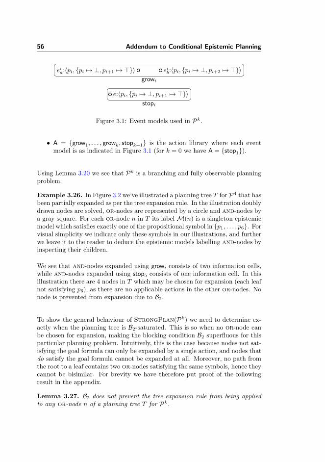
56 Addendum to Conditional Epistemic Planning

eia:〈pi, {pi 7→ ⊥, pi+1 7→ >}〉 eib:〈pi, {pi 7→ ⊥, pi+2 7→ >}〉growi

e:〈pi, {pi 7→ ⊥, pi+1 7→ >}〉stopi

Figure 3.1: Event models used in Pk.

• A = {grow1, . . . , growk, stopk+1} is the action library where each eventmodel is as indicated in Figure 3.1 (for k = 0 we have A = {stop1}).

Using Lemma 3.20 we see that Pk is a branching and fully observable planningproblem.

Example 3.26. In Figure 3.2 we’ve illustrated a planning tree T for P4 that hasbeen partially expanded as per the tree expansion rule. In the illustration doublydrawn nodes are solved, or-nodes are represented by a circle and and-nodes bya gray square. For each or-node n in T its labelM(n) is a singleton epistemicmodel which satisfies exactly one of the propositional symbol in {p1, . . . , p6}. Forvisual simplicity we indicate only these symbols in our illustrations, and furtherwe leave it to the reader to deduce the epistemic models labelling and-nodes byinspecting their children.

We see that and-nodes expanded using growi consists of two information cells,while and-nodes expanded using stop5 consists of one information cell. In thisillustration there are 4 nodes in T which may be chosen for expansion (each leafnot satisfying p6), as there are no applicable actions in the other or-nodes. Nonode is prevented from expansion due to B2.

To show the general behaviour of StrongPlan(Pk) we need to determine ex-actly when the planning tree is B2-saturated. This is so when no or-node canbe chosen for expansion, making the blocking condition B2 superfluous for thisparticular planning problem. Intuitively, this is the case because nodes not sat-isfying the goal formula can only be expanded by a single action, and nodes thatdo satisfy the goal formula cannot be expanded at all. Moreover, no path fromthe root to a leaf contains two or-nodes satisfying the same symbols, hence theycannot be bisimilar. For brevity we have therefore put proof of the followingresult in the appendix.

Lemma 3.27. B2 does not prevent the tree expansion rule from being appliedto any or-node n of a planning tree T for Pk.

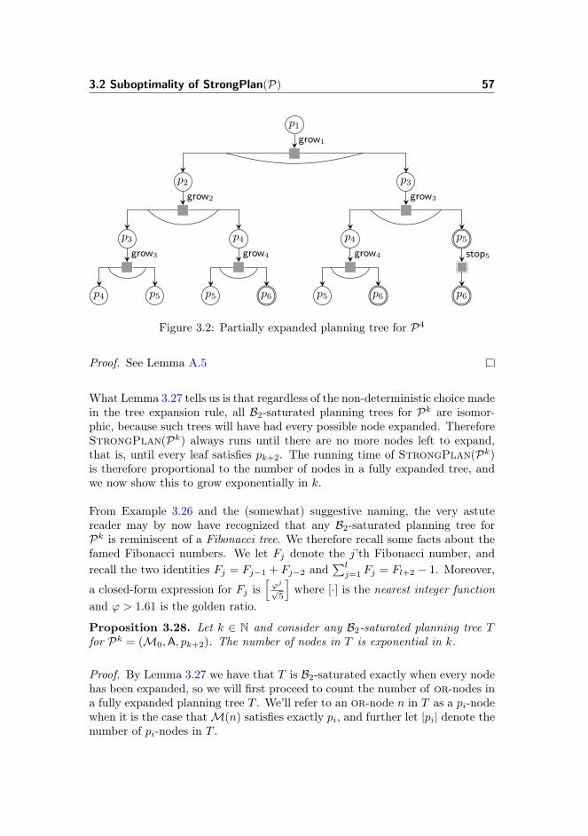
3.2 Suboptimality of StrongPlan(P) 57

p1

p2 p3

p3 p4 p4 p5

p4 p5 p5 p6 p5 p6

grow1

grow2 grow3

grow3 grow4 grow4

p6

stop5

Figure 3.2: Partially expanded planning tree for P4

Proof. See Lemma A.5

What Lemma 3.27 tells us is that regardless of the non-deterministic choice madein the tree expansion rule, all B2-saturated planning trees for Pk are isomor-phic, because such trees will have had every possible node expanded. ThereforeStrongPlan(Pk) always runs until there are no more nodes left to expand,that is, until every leaf satisfies pk+2. The running time of StrongPlan(Pk)is therefore proportional to the number of nodes in a fully expanded tree, andwe now show this to grow exponentially in k.

From Example 3.26 and the (somewhat) suggestive naming, the very astutereader may by now have recognized that any B2-saturated planning tree forPk is reminiscent of a Fibonacci tree. We therefore recall some facts about thefamed Fibonacci numbers. We let Fj denote the j’th Fibonacci number, andrecall the two identities Fj = Fj−1 + Fj−2 and

∑lj=1 Fj = Fl+2 − 1. Moreover,

a closed-form expression for Fj is[ϕj

√5

]where [·] is the nearest integer function

and ϕ > 1.61 is the golden ratio.

Proposition 3.28. Let k ∈ N and consider any B2-saturated planning tree Tfor Pk = (M0,A, pk+2). The number of nodes in T is exponential in k.

Proof. By Lemma 3.27 we have that T is B2-saturated exactly when every nodehas been expanded, so we will first proceed to count the number of or-nodes ina fully expanded planning tree T . We’ll refer to an or-node n in T as a pi-nodewhen it is the case thatM(n) satisfies exactly pi, and further let |pi| denote thenumber of pi-nodes in T .

58 Addendum to Conditional Epistemic Planning

Since no action adds a p1-node, we have immediately from the initial state that|p1| = 1. We now settle the number of or-nodes resulting from applying thetree expansion rule in some pi node. When stopk+1 is applicable the result is apk+2-node, and furthermore for 1 ≤ i ≤ k we have that when growi is applicable,the result is a pi+1-node and a pi+2-node. To determine |p2|, we have in the caseof k = 0 that |p2| = 1 due to stop1. Otherwise when k > 0, then we have fromgrow1 that |p2| = |p1|+ |p0| which equals 1 as there are no p0-nodes. Summingup we have that |p1| = 1 and |p2| = 1 for any k.

For 3 ≤ j ≤ k+2 we have that one pj-node is added for each pj−1-node and onefor each pj−2-node; with the case of j = k + 2 combining the single node fromgrowk and the single node from stopk+1. Put on a symbolic form this means|pj | = |pj−1| + |pj−2|. Observe now that |p1| = F1, |p2| = F2, and since |pj |is identical to the Fibonnaci recurrence we arrive at |pj | = |pj−1| + |pj−2| =Fj−1 + Fj−2 = Fj .

From Lemma A.1 we have that every or-node in T satisfies exactly one propo-sitional symbol. Therefore the total number of or-nodes in T is precisely givenby |p1| + · · · + |pk+2| = F1 + · · · + Fk+2 = Fk+4 − 1 =

[ϕk+4

√5

]− 1. Since T is

a planning tree there is at least one more or-node than there are and-nodes,hence the number of and-nodes in T is at most Fk+4 − 2, thus we have

[ϕk+4

√5

]− 1 ≤ |T | ≤ 2

[ϕk+4

√5

]− 3 as ϕ > 1⇒

|T | = Θ(ck) for some c > 1

, thereby showing that the number of nodes in T is exponential in k.

Corollary 3.29. StrongPlan is an exponential time algorithm for the solu-tion existence problem for Pk.

In an alternative formulation of Pk we can consider {p1, . . . , pk+2} as encodingan integer, and construct actions that capture integer arithmetic — we use suchactions in Section 3.4.3. A B2-saturated planning tree for this alternative versioncontains F2k+2+2 or-nodes, and so the running time of StrongPlan is in thiscase doubly exponential in k, coinciding roughly with the upper bound for fullyobservable planning problems that we presented at the start of this section. Asshown later in Theorem 3.53, this implies that StrongPlan is asymptoticallysuboptimal for deciding whether a solution exists.

3.3 Optimal Decision Procedures 59

3.3 Optimal Decision Procedures

In this section we introduce asymptotically optimal decision procedures for an-swering the solution existence problem, with optimality being shown by theresults of Section 3.4. We put the tools of Section 3.1 to use here, both forshowing correctness of this procedure and for bounding the resources used. Theupper bounds differ for each of the four types of planning problems mentionedin Section 3.1.5. For planning problems that are branching we replace plan-ning trees with planning graphs, so that our algorithm can avoid expandingredundant nodes. Non-branching problems are simpler because we only need todetermine whether a sequential plan exists, and so we can use a strategy thatrequires fewer space resources in this case.

3.3.1 Replacing Planning Trees

As illustrated in Section 3.2 we risk adding an exponential number of bisimilarnodes to the planning tree when using this as our underlying data structure. Wecan eliminate this behaviour from our decision procedure by identifying nodesthat, loosely stated, contain the same information. Foregoing the extraction ofplans from planning trees, the nodes we seek to identify are those that “behavethe same” when considering in tandem the tree expansion rule (Definition 2.18)and the notion of solved nodes (Definition 2.21). This means that for two nodesn, n′ to be identified we must have thatM(n) andM(n′) are modally equivalent(Definition 3.3) and further, if we take any event model E , the nodes added bythe tree expansion rule using n and E are modally equivalent to the nodes addedusing n′ and E . To incorporate this fact into StrongPlan one might attemptto augment B2 further and keep employing planning trees. However, a morerewarding approach is to do away with trees as whole, and instead turn to amore suited form of graph.

Definition 3.30. A planning graph G = (N,M,E, n0) is a bipartite, rooted,directed and labelled graph. N and M are disjoint sets of nodes, where Ndenotes a set of or-nodes and M a set of and-nodes. The or-node n0 ∈ N isthe root, also denoted root(G). Each node v of G is labelled by an epistemicmodelM(v). Each edge (n,m) ∈ E with n ∈ N and m ∈ M is labelled by anevent model E(n,m). We require that there is a path from n0 to every othernode in G (implying that G is weakly connected).

Given a planning problem P = (M0,A, φg), a planning graph G = (N,M,E, n0)for P is one in which M(n0) = M0 and where every edge (n,m) from an or-node to an and-node has E(n,m) ∈ A. The initial planning graph for P is

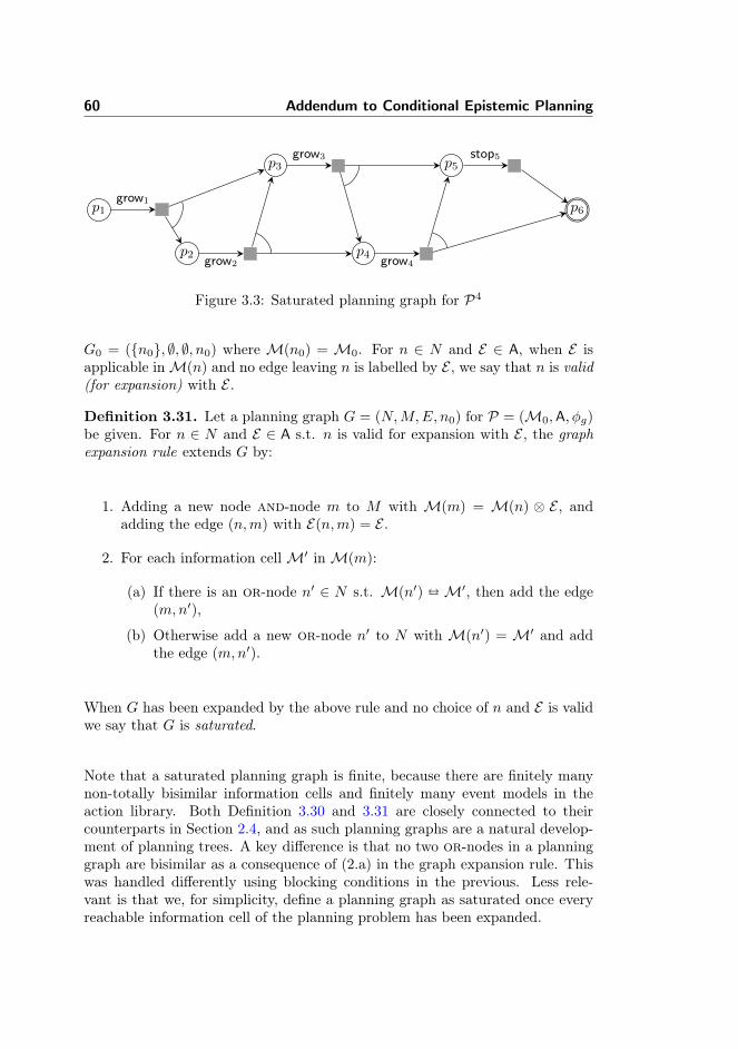
60 Addendum to Conditional Epistemic Planning

p1

p2

p3

p4

p5

p6grow1

grow2

grow3

grow4

stop5

Figure 3.3: Saturated planning graph for P4

G0 = ({n0}, ∅, ∅, n0) where M(n0) = M0. For n ∈ N and E ∈ A, when E isapplicable inM(n) and no edge leaving n is labelled by E , we say that n is valid(for expansion) with E .

Definition 3.31. Let a planning graph G = (N,M,E, n0) for P = (M0,A, φg)be given. For n ∈ N and E ∈ A s.t. n is valid for expansion with E , the graphexpansion rule extends G by:

1. Adding a new node and-node m to M with M(m) = M(n) ⊗ E , andadding the edge (n,m) with E(n,m) = E .

2. For each information cellM′ inM(m):

(a) If there is an or-node n′ ∈ N s.t. M(n′) -M′, then add the edge(m,n′),

(b) Otherwise add a new or-node n′ to N with M(n′) = M′ and addthe edge (m,n′).

When G has been expanded by the above rule and no choice of n and E is validwe say that G is saturated.

Note that a saturated planning graph is finite, because there are finitely manynon-totally bisimilar information cells and finitely many event models in theaction library. Both Definition 3.30 and 3.31 are closely connected to theircounterparts in Section 2.4, and as such planning graphs are a natural develop-ment of planning trees. A key difference is that no two or-nodes in a planninggraph are bisimilar as a consequence of (2.a) in the graph expansion rule. Thiswas handled differently using blocking conditions in the previous. Less rele-vant is that we, for simplicity, define a planning graph as saturated once everyreachable information cell of the planning problem has been expanded.

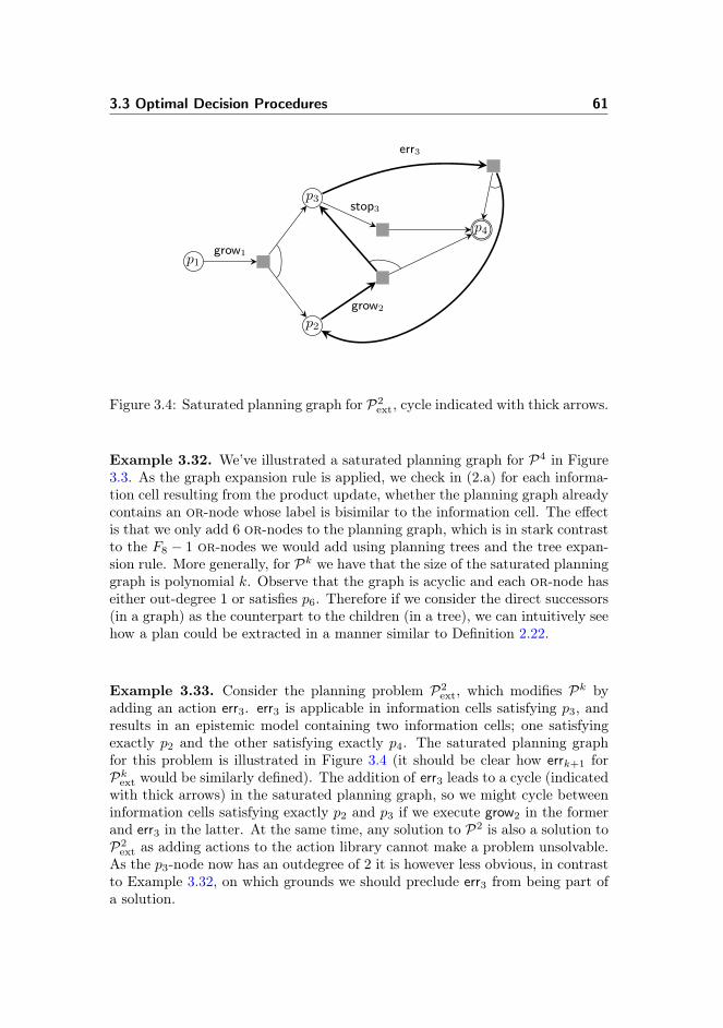
3.3 Optimal Decision Procedures 61

p1

p2

p3

p4

grow1

grow2

stop3

err3

Figure 3.4: Saturated planning graph for P2ext, cycle indicated with thick arrows.

Example 3.32. We’ve illustrated a saturated planning graph for P4 in Figure3.3. As the graph expansion rule is applied, we check in (2.a) for each informa-tion cell resulting from the product update, whether the planning graph alreadycontains an or-node whose label is bisimilar to the information cell. The effectis that we only add 6 or-nodes to the planning graph, which is in stark contrastto the F8 − 1 or-nodes we would add using planning trees and the tree expan-sion rule. More generally, for Pk we have that the size of the saturated planninggraph is polynomial k. Observe that the graph is acyclic and each or-node haseither out-degree 1 or satisfies p6. Therefore if we consider the direct successors(in a graph) as the counterpart to the children (in a tree), we can intuitively seehow a plan could be extracted in a manner similar to Definition 2.22.

Example 3.33. Consider the planning problem P2ext, which modifies Pk by

adding an action err3. err3 is applicable in information cells satisfying p3, andresults in an epistemic model containing two information cells; one satisfyingexactly p2 and the other satisfying exactly p4. The saturated planning graphfor this problem is illustrated in Figure 3.4 (it should be clear how errk+1 forPkext would be similarly defined). The addition of err3 leads to a cycle (indicatedwith thick arrows) in the saturated planning graph, so we might cycle betweeninformation cells satisfying exactly p2 and p3 if we execute grow2 in the formerand err3 in the latter. At the same time, any solution to P2 is also a solution toP2

ext as adding actions to the action library cannot make a problem unsolvable.As the p3-node now has an outdegree of 2 it is however less obvious, in contrastto Example 3.32, on which grounds we should preclude err3 from being part ofa solution.

62 Addendum to Conditional Epistemic Planning

To handle the general case, we must be able to determine whether a planninggraph admits a solution when it is cyclic and the outdegree of or-nodes isgreater than 1. To this end we will look for an acyclic subgraph satisfyingcertain criteria that guarantees the existence of a strong solution.

Definition 3.34. Let a saturated planning graph G = (N,M,E, n0) for P =(M0,A, φg) be given. A solved subgraph of G for n′0 ∈ N is a subgraph G′ =(N ′,M ′, E′, n′0) of G satisfying the following criteria.

C1 n′0 is the single source node (indegree is 0), and every node in G′ is reachablefrom n′0,

C2 G′ is acyclic,

C3 For each n′ ∈ N ′: the outdegree of n′ is 0 if M(n′) |= φg (a goal node is asink), and otherwise the outdegree of n′ is 1 and this outgoing edge hasthe same label as in G,

C4 For each m′ ∈ M ′: (m′, n′) ∈ E′ iff (m′, n′) ∈ E (outgoing edges of and-nodes are exactly as in G).

We say that G is solved if there exists a solved subgraph of G for n0.

Observe that n′0 can be any or-node of the saturated planning graph. We alsorequire the following intuitive definition used in the results shown in Appendix3.3.

Definition 3.35. Given a solved subgraph G′ = (N ′,M ′, E′, n′0), we define forany node v′ of G′ its height h(v′) recursively by:

• If v′ ∈ N ′ andM(v′) |= φg then h(v′) = 0,

• If v′ ∈ N ′ andM(v′) 6|= φg, then h(v′) = h(m′) + 1 where m′ is the singlethe direct successor of v′, and

• If v′ ∈ M ′, then h(v′) = max(h(n′1), . . . , h(n′k)) + 1 where n′1, . . . , n′k arethe direct successors of v′.

From C2 we have that a solved subgraph G′ is an acyclic subgraph G and soG′ contains no paths of infinite length. C3 means we assign to each reachableinformation cell (not satisfying the goal) a single action, whose expansion isalso contained in G′ by virtue of C4, hence G′ faithfully represents the graphexpansion rules applied when saturating G. Taking into account C1, G′ fully

3.3 Optimal Decision Procedures 63

describes the actions an agent must take from the initial state in order to reacha sink, regardless of what contingency arise during execution. In this sense asolved subgraph contains all the information necessary in order to synthesise aplan, and as such plays the same role as a planning tree whose root is solved.

3.3.2 Working with Planning Graphs

In showing correctness of the decision procedure we develop in Section 3.3.3, wefirst show that notion of a solved planning tree coincides with that of a solvedsubgraph.

Lemma 3.36. Let a planning problem P = (M0,A, φg) be given. There existsa B2-saturated planning tree for P whose root is solved iff the saturated planninggraph G for P is solved.

Proof. Assume that we’re given a B2-saturated planning tree T for P such thatroot(T ) is solved. We must show that the saturated planning graph for P issolved. We outline how this is shown, with a full proof of this direction beingavailable in the proof of Lemma A.6 in Appendix A.2. The proof proceedsby constructing from T a graph G′ which constitutes a solved subgraph of Gup to bisimilarity. The first step is pruning T so that it contains only solvednodes, which implies that or-nodes in T have outdegree 0 if they satisfy φg andotherwise they have outdegree 1. Starting from the leaves of T , we iterativelymove up the planning tree, extending G′ with the or-nodes and and-nodesencountered with the proviso that no two bisimilar or-nodes are added to G′.In this way, the children of any node we process in T are guaranteed to (at least)have a bisimilar partner in G′, allowing us construct G′ so that the edges in Tare matched up to bisimilarity.

With a few modifications, we can map G′ to a subgraph of G which satisfiesC1 and C2. That this mapping satisfies C3 follows from the initial pruning ofT . Showing this mapping satisfies C4 is done on the basis that both the treeexpansion rule and graph expansion rule use the product update operation. Thisimplies the existence of a solved subgraph of G for P thereby concluding thisdirection.

We only sketch the other direction, whose proof is conceptually more simple.It is essentially the inverse of the procedure we gave above, that is, we take asolved subgraph ofG, and from this construct a planning tree (up to bisimilarity)whose root is solved. Assuming that we’re given a solved subgraph G′ of G, wemanipulate it by repeatedly splitting an or-node n whose indegree is greaterthan 1, until no such n exists. When splitting a node, we add a new node n′

64 Addendum to Conditional Epistemic Planning

whose label isM(n), and one incoming edge of n is modified so that it insteadpoints to n′. Below n′ we add a copy of the acyclic subgraph that has n asits root. As G′ initially satisfies C2 we have that the split operation preservesacyclicity. Furthermore, every sink of G′ remains a sink and the source is neversplit as its indegree is 0. Therefore once every or-node in G′ has indegree atmost 1, it constitutes a planning tree (up to bisimilarity) whose root is theroot of G′, and whose leaves are the sinks in G′ meaning that each leaf satisfiesφg. Again, the correspondence between the graph expansion rule and the treeexpansion rule means this procedure in fact gives a B2-saturated planning treefor P.

Having established the result above, we are still in need of a procedure for deter-mining whether a saturated planning graph is solved. To this end, we adapt thealgorithm StrongPlan found in [Cimatti et al., 2003] to our setting. WhileStrongPlan assumes a fully observable domain, the extension to partial ob-servability is straightforward. Roughly speaking, StrongPlan starts from anempty plan, and in each iteration of its main loop extends this plan by assigningactions to states. There are two requirements for a state to be assigned an ac-tion. First, a state is at most assigned one action (ensured by PruneStates).Second, the action must guarantee that its outcomes are either goal states orstates for which an action has already been assigned (achieved using Strong-PreImage). Keeping in mind these two requirements, we now introduce theprocedure SolvedSubgraph.

Definition 3.37. Let a saturated planning graph G = (N,M,E, n0) be given.For any N ′ ⊆ N , we define the predicate Solved(m,G,N ′) ⇔ (∀(m,n) ∈ E :n ∈ N ′).

Informally we have that Solved(m,G,N ′) holds if an action that produces mis guaranteed to lead to one of the information cells in N ′. As such, Solvedserves to determine whether the second requirement mentioned above holds inour setting, and is directly put to work in line 6 of SolvedSubgraph. The firstrequirement is achieved in line 4 where we ignore any or-node already containedin G′. The input of SolvedSubgraph is a saturated planning graph and a goalformula.

3.3 Optimal Decision Procedures 65

SolvedSubgraph(G = (N,M,E, n0), φg)

1 N ′ = {n ∈ N | M(n) |= φg}, M ′ = ∅, E′ = ∅2 G′ = (N ′,M ′, E′)3 while G′ is modified by the following4 Nus = N \N ′ � Unsolved or-nodes5 for each n ∈ Nus

6 if n has a direct successor m in G s.t. Solved(m,G,N ′) then7 Add n, m, (n,m) and (m,n1), . . . , (m,nk) to G′

where and n1, . . . , nk are the direct successors of m in G.� N ′,M ′, E′ of G′ are modified

8 return G′

The following result is oblivious to the actual cost of the operations in Solved-Subgraph, meaning that we simply count the number of high-level steps de-scribed. We rectify this shortcoming later when it becomes prudent to ouranalysis.

Lemma 3.38. The number of steps used in SolvedSubgraph is polynomialin |N |.

Proof. We count the number of iterations in the nested loop construction. Foreach iteration starting at line 3, we have that the loop ends unless G′ is modifiedin line 7. Each iteration modifying G′ adds at least one node in N to N ′.Therefore the number of iterations modifying N ′ is at most the number of nodesin N . Furthermore the loop in line 5 requires at most N iterations, and so line7 is reached at most |N |2 times.

We will use Gi to denote the graph produced after i iterations of the loop inline 3 of SolvedSubgraph. Observe that as SolvedSubgraph never removesnodes, we have that Gi is a subgraph of Gi+1. The following result essentiallystates that each or-node n∗ we add to G′ in line 7 can be composed withsubcomponents of G′ to form a solved subgraph of G for n∗.

Lemma 3.39. Given a saturated planning graph G = (N,M,E, n0) for P =(M0,A, φg), and let Gi = (Ni,Mi, Ei). Further, let n∗ ∈ (N \ Ni) s.t. n∗ hasa direct successor m∗ in G with Solved(m∗, G,Ni), and where n1, . . . , ny ∈ Nidenotes the direct successors of m∗ (see also Figure 3.5). If for each x s.t.1 ≤ x ≤ y there exists a solved subgraph of Gi for nx, then there exists a solvedsubgraph of G for n∗.

Proof. We form the graph G∗ that is indicated in Figure 3.5. We then showthat this graph satisfies the four criteria for being a solved subgraph of G forn∗. A full proof is given when showing Lemma A.8 in Appendix A.2.

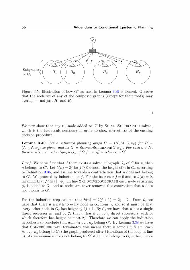
66 Addendum to Conditional Epistemic Planning

H1

n1

H2

n2 · · ·

Hx

nx · · ·

Hy

ny

m∗

n∗

Subgraphsof Gi

Figure 3.5: Illustration of how G∗ as used in Lemma 3.39 is formed. Observethat the node set of any of the composed graphs (except for their roots) mayoverlap — not just H1 and H2.

We now show that any or-node added to G′ by SolvedSubgraph is solved,which is the last result necessary in order to show correctness of the ensuingdecision procedure.

Lemma 3.40. Let a saturated planning graph G = (N,M,E, n0) for P =(M0,A, φg) be given, and let G′ = SolvedSubgraph(G,φg). For each n ∈ N ,there exists a solved subgraph Gs of G for n iff n belongs to G′.

Proof. We show first that if there exists a solved subgraph Gs of G for n, thenn belongs to G′. Let h(n) = 2j for j ≥ 0 denote the height of n in Gs accordingto Definition 3.35, and assume towards a contradiction that n does not belongto G′. We proceed by induction on j. For the base case j = 0 and so h(n) = 0,meaning thatM(n) |= φg. In line 2 of SolvedSubgraph each node satisfyingφg is added to G′, and as nodes are never removed this contradicts that n doesnot belong to G′.

For the induction step assume that h(n) = 2(j + 1) = 2j + 2. From C1 wehave that there is a path to every node in Gs from n, and so it must be thatevery other node in Gs has height ≤ 2j + 1. By C3 we have that n has a singledirect successor m, and by C4 that m has n1, . . . , ny direct successors, each ofwhich therefore has height at most 2j. Therefore we can apply the inductionhypothesis to conclude that each n1, . . . , ny belong G′. By Lemma 3.38 we havethat SolvedSubgraph terminates, this means there is some i ∈ N s.t. eachn1, . . . , ny belong to Gi (the graph produced after i iterations of the loop in line3). As we assume n does not belong to G′ it cannot belong to Gi either, hence

3.3 Optimal Decision Procedures 67

n ∈ (N \Ni). But we now have n ∈ Nus and that n and its direct successor msatisfy the conditions condition in line 6 of SolvedSubgraph, and so it followsthat n belongs to Gi+1, thus contradicting that n does not belong to G′.

Turning to the converse, we now show that if n belongs to G′, then there existsa solved subgraph Gs of G for n. We proceed by induction on the number iof iterations by the loop in line 3. For the base case assume that 0 iterationshave been made, which implies that n ∈ {n′ ∈ N | M(n′) |= φg}. ThereforeM(n) |= φg, and so ({n}, ∅, ∅, n) is a solved subgraph of G for n. For theinduction step assume that i + 1 iterations has been made. If n was added initeration ≤ i, then the induction hypothesis immediately gives that there existsa solved subgraph for n. We can therefore assume that n was added in iterationi + 1, meaning that n ∈ (N \ Ni). From line 6 it follows that n has a directsuccessor m in G with Solved(m∗, G,Ni), and where n1, . . . , ny ∈ Ni are thedirect successors ofm∗. For 1 ≤ x ≤ y we have that nx was added in an iteration≤ i, and so by the induction hypothesis there exists a solved subgraph Hx ofGi for nx. This means we can apply Lemma 3.39 to conclude that there existsa solved subgraph of G for n, thus concluding the induction step.

3.3.3 Deciding Whether a Solution Exists

We present an optimal decision procedure for the solution existence problem,and show that this procedure is both sound and complete.

SolutionExists(P = (M0,A, φg))

1 Construct the initial planning graph G = ({n0}, ∅, ∅, n0) for P withM(n0) =M0.2 Repeatedly apply the graph expansion rule until G is saturated, with the addition

that labels of or-nodes are bisimulation contracted.3 Answer YES if n0 belongs to SolvedSubgraph(G,φg), otherwise answer NO.

In line 2 of SolutionExists we make sure that the labels of or-nodes in theplanning graph represent contraction-minimal information cells. Doing this in-curs little overhead when constructing the saturated planning graph, and ensuresthat the epistemic models are of reasonable size.

Theorem 3.41. SolutionExists is a sound and complete decision procedurefor the solution existence problem.

Proof. Soundness means that if SolutionExists(P) answers YES, then thereexists a solution to P. When n0 belongs to SolvedSubgraph(G,φg), then it

68 Addendum to Conditional Epistemic Planning

follows from Lemma 3.40 that G is solved. By Lemma 3.36 we therefore havethat there exists a planning tree for P whose root is solved. Applying Theorem2.24 it follows that there exists a solution to P as required. To show complete-ness, assume that there exists a solution to P. By Theorem 2.25 this implies theexistence of B2-saturated planning tree for P whose root is solved. By Lemma3.36 we therefore have that G is solved, and applying Lemma 3.40 it follows thatn0 belongs to SolvedSubgraph(G,φg). Therefore SolutionExists answersYES as required.

We now make our analysis of the running time of SolutionExists more con-crete, namely as a function of the size of the input planning problem. For aplanning problem P = (M0,A, φg) its size is given in the obvious way, viz.|P| = |M0|+

∑E∈A |E|+ |φg| (see Section 3.1.3 for more on the size of inputs).

Theorem 3.42. The solution existence problem is in 2EXP.

Proof. Given any planning problem P = (M0,A, φg) on P we show that the

running time of SolutionExists(P) is O(22ik

) where i = |P| and k is someconstant. From Lemma 3.11 the number of worlds in any contraction-minimalinformation cell on P is at most 2|P |. As |M0| + |P | ≤ i this means anyinformation cell of an or-node in the saturated planning graph has size at mostO(2i).

We now consider the operations of the algorithm whose running time dependson the size of the input, namely graph expansion and bisimulation contraction.When applying the graph expansion rule we need to determine applicability, amodel checking task, and compute the product update. Important here is thatthe size of any precondition and any event model is at most i. Using Proposition3.15 and Proposition 3.16 and the fact that any information cell has size atmost O(2i), this means we can compute the application of any graph expansionrule using time polynomial in 2i. For bisimulation contraction, we have byLemma 3.9 a simple characterization of bisimilar worlds in an information cell.Therefore, a contraction-minimal model can be obtained by removing worldsof an information cell until no two have the same label. From |M0| ≤ i andthe fact that or-nodes are bisimulation contracted immediately, computing thebisimulation contraction of any information cell can be done in time polynomialin 2i.

By definition of the graph expansion rule, no two or-nodes in the planning graphare bisimilar and furthermore each or-node is expanded at most once for eachaction in the action library. With the number of non-bisimilar information cellson P being at most 22i

by Lemma 3.12, it follows that the number of or-nodesin the saturated planning graph is at most 22i

. Moreover, since |A| ≤ i and

3.3 Optimal Decision Procedures 69

each expansion requires time polynomial in 2i, this means there is a constantk1 such that O(2(2i)k1

) is an upper bound on the time used for constructing thesaturated planning graph in line 2 of SolutionExists.

The initial computation of nodes satisfying φg (line 1 of SolvedSubgraph)requires solving at most 22i

model checking tasks. The input of each task is acontraction-minimal information cell of size at most O(2i) and a formula of sizeat most i. The remaining steps of SolvedSubgraph can be computed in timepolynomial in the size of the saturated planning graph by Lemma 3.38, andso there are at most 22i

such steps. From these facts and Proposition 3.15 itfollows that there is exists a constant k2 such that O(2(2i)k2

) is an upper boundon the time required for computing line 3 of SolutionExists.

Consequently we have that the running time of SolutionExists(P) is

O(2(2i)k1+ 2(2i)k2

)

. Letting k = max(k1, k2) this reduces to O(22ik

), and by Theorem 3.41 wetherefore have that the solution existence problem is in 2EXP.

It is worth pointing out that it is the number of propositions in P which is themost significant factor in the asymptotic analysis of SolutionExists. More-over, this analysis also reveals that it is the number of non-totally bisimilarinformation cells that prevents a better upper bound on the running time ofSolutionExists. In fully observable planning problems we have that anyreachable information cell is a singleton. This means that the number of non-totally bisimilar information cells for such planning problems is at most 2i byLemma 3.10. From these facts we can readily establish the following result.

Theorem 3.43. The solution existence problem for fully observable planningproblems is in EXP.

[Littman, 1997] shows that the solution existence problem for fully observableautomated planning problems is in EXP, and [Rintanen, 2004] shows the case of2EXP membership under the assumption of partial observability. The member-ship argument in [Littman, 1997] is by using results on the complexity of solvingMDPs [Condon, 1992], showing this to be polynomial in the number of states.As a fully observable planning problem may induce an exponentially sized MDP,this implies the solution existence problem is in EXP. A similar argument ismade in [Rintanen, 2004], though instead with reference to the algorithm in[Cimatti et al., 2003].

70 Addendum to Conditional Epistemic Planning

3.3.4 Non-Branching Problems

Recall that for a non-branching planning problem P, we have for any reachableinformation cell of P that any action in the action library is non-branching(see Definition 3.18). So if P is solvable, then a solution exists which is simplya sequence of actions. However, this observation does not improve the upperbound on SolutionExists, since the number of non-totally bisimilar reachableinformation cells of P remains the same as in the case of branching problems —we need another approach. At the same time, it might still be that the length of asolution is (doubly) exponential in the size of P, subject to whether the planningproblem is fully or partially observable. Therefore, if the solution existenceproblem had been a function problem (i.e. its output was required to be thestrong solution, not just YES or NO), we’d need to store these very large plansand so had no hope of improving the upper bounds shown for SolutionExists.

We now sketch a non-deterministic procedure that decides the solution existenceproblem for any partially observable and non-branching planning problem P =(M0,A, φg) on P . Starting fromM0, ifM0 |= φg answer YES, otherwise non-deterministically pick an applicable action E ∈ A, and compute the bisimulationcontraction ofM =M0 ⊗ E which is by definition an information cell. Repeatthis process until either M |= φg in which case the answer is YES, or 22|P |

non-deterministic choices have been made in which case the answer is NO.

This procedure is sound, for if the answer is YES then there is a solution toP consisting of the sequence of actions chosen, each of which are applicableand whose execution is guaranteed to result in an information cell satisfyingthe goal. It is complete for the following reasons. A solution to this type ofplanning problem can always be formulated as a sequence of actions, and thereare at most 22|P | non-bisimilar information cells on P by Lemma 3.12. Thereforewhen a solution consists of more than 22|P | actions, it will necessarily reach twobisimilar information cells. Since both applicability and the product updateoperation are invariant under bisimulation (Corollary 3.7 and Lemma 3.8), thismeans that for a given solution, removing a sequence of actions between any twobisimilar information cells will also be a solution. Consequently, if P is solvablethen there exists a solution using at most 22|P | actions.

Theorem 3.44. The solution existence problem for non-branching and partiallyobservable planning problems is in EXPSPACE.

Proof. Given any partially observable and non-branching planning problem P =(M0,A, φg) on P , and let i = |P|. We show that the procedure outlined aboverequires no more than O(2i

k

) space for some constant k. At each step of thecomputation we need to store a single contraction-minimal information cell, as

3.3 Optimal Decision Procedures 71

well as the number of choices that have been made so far. By Lemma 3.11 wehave that a contraction-minimal information cell contains at most 2|P | worlds, soas |P | ≤ i this requires at most O(2i) space. As in the proof of Theorem 3.42, wecan therefore compute applicability and the product update operation in timepolynomial in 2i, and so this also bounds the amount of space used. Using 2|P |

bits we can represent any integer up to 22|P | , meaning this is the number of bitsrequired to keep of track of how many choices have been made. Therefore theprocedure uses only O(2i

k

) space for some constant k, hence the procedure isin NEXPSPACE and consequently in EXPSPACE by Savitch’s theorem. Fromsoundness and completeness of the procedure the result follows.

In the case of non-branching and fully observable planning problems, we needonly to repeat the above procedure until 2|P | non-deterministic choices havebeen made as this is the number of non-bisimilar singleton information cells onP (Lemma 3.10). Storing a singleton information cell requires no more thanO(i) space, and using |P | ≤ i bits we can keep track of how many choices havebeen made. From this the following result is established as in the proof above(NPSPACE = PSPACE by Savitch’s theorem), except that we must also requireactions to be static (preconditions and postconditions belong to LEL(P )) andthe goal formula to belong to LEL(P ). Otherwise the model checking task mayrequire time exponential in the size of the planning problem, which poses therisk of violating the polynomial space bound. As discussed in Section 3.1.4,if the PSPACE algorithm due [Aucher and Schwarzentruber, 2012] could bemodified to handle postconditions, the following result would be voided of theserequirements.

Theorem 3.45. The solution existence problem for non-branching and fullyobservable planning problems is in PSPACE, if each action in the action libraryis static and the goal formula is in LEL(P ).

The membership algorithm we sketch here is nondeterministic and uses substan-tially less space than there are reachable information cells. The key insight uponwhich this is based is due to [Bylander, 1994], where the solution existence prob-lem for automated planning was shown to be in PSPACE. This insight was alsoused in [Haslum and Jonsson, 1999] where automated planning problems withpartial observability and deterministic actions was shown to be in EXPSPACE.[Bolander and Andersen, 2011] shows that the solution existence problem in thesingle-agent case is decidable, though the exact complexity is not settled.

As mentioned above, the reason we can obtain better upper bounds is becausewe’re working with a decision problem, and so need not store the entire plan.6

6Whether we do in fact achieve a better upper bound is subject to whether PSPACE ?= EXP

and EXPSPACE ?= 2EXP.

72 Addendum to Conditional Epistemic Planning

Nonetheless, this approach is not completely without practical merit when plan-ning and execution is interleaved. Say for instance an agent is given a partiallyobservable and non-branching planning problem that she must solve, and canapply an EXPSPACE algorithm that decides the solution existence problem.By picking an action applicable in the initial state, the agent can query thealgorithm and ask whether there exists a strong solution from the resultinginformation cell. If so the agent can safely execute this action, as it will notrender her unable to solve the problem. By repeating this process (for the re-sulting information cells) until the goal is reached, the agent need not storethe entire plan, and so is able to eventually reach a goal state using at mostspace exponential in the size of the planning problem. This approach can ofcourse be generalized to using a constant number of actions when applying theEXPSPACE algorithm.

3.4 Simulating Turing Machines

In the previous section we gave sound and complete decision procedures for thesolution existence problem, and further analyzed their worst-case case complex-ity. Next on our agenda is to show that each of the four variants of the solutionexistence problem we consider are among the hardest problems in their indi-cated complexity class. This means we cannot hope to find better proceduresfor the solution existence problem than those given above.

The computational complexity of automated planning problems has been ex-tensively studied. [Bylander, 1994] shows the problem of determining whethera solution exists to a classical planning problem is PSPACE-Complete. Addingnondetermism makes the problem EXP-Complete as proved in [Littman, 1997],and with partial observability we have EXPSPACE completeness due to [Haslumand Jonsson, 1999]. Lastly, [Rintanen, 2004] shows that with both partial ob-servability and nondeterminism the problem is 2EXP-Complete. Both [Littman,1997] and [Haslum and Jonsson, 1999] establish their results by reductions to de-cision problems known to be complete for their respective classes. The approachof [Bylander, 1994] is more direct in that planning problems are constructed tosimulate the transitions of a polynomial space bounded DTM on a given input.

The most generic approach is found [Rintanen, 2004] (and is put on full dis-play in [Rintanen, 2005]), where planning problems are constructed to simulateDTMs and ATMs either with polynomial or exponential space bounds. Thetwo key insights of this work is that nondeterminism can be used to simulatealternating computation, and that partial observability can be used to exponen-tially increase the number of tape cells that can be represented in a state. What

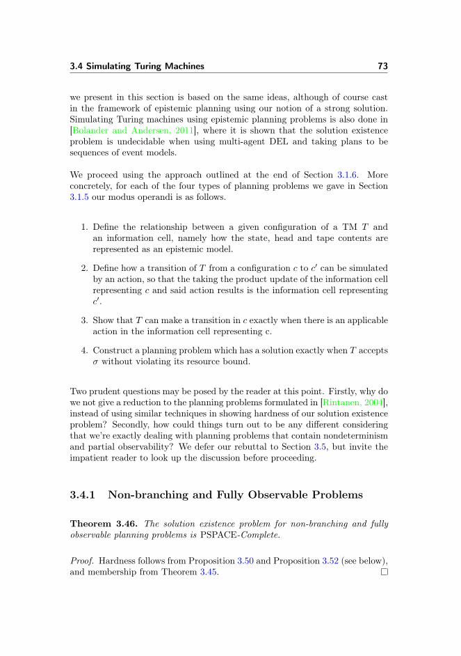
3.4 Simulating Turing Machines 73

we present in this section is based on the same ideas, although of course castin the framework of epistemic planning using our notion of a strong solution.Simulating Turing machines using epistemic planning problems is also done in[Bolander and Andersen, 2011], where it is shown that the solution existenceproblem is undecidable when using multi-agent DEL and taking plans to besequences of event models.

We proceed using the approach outlined at the end of Section 3.1.6. Moreconcretely, for each of the four types of planning problems we gave in Section3.1.5 our modus operandi is as follows.

1. Define the relationship between a given configuration of a TM T andan information cell, namely how the state, head and tape contents arerepresented as an epistemic model.

2. Define how a transition of T from a configuration c to c′ can be simulatedby an action, so that the taking the product update of the information cellrepresenting c and said action results is the information cell representingc′.

3. Show that T can make a transition in c exactly when there is an applicableaction in the information cell representing c.

4. Construct a planning problem which has a solution exactly when T acceptsσ without violating its resource bound.

Two prudent questions may be posed by the reader at this point. Firstly, why dowe not give a reduction to the planning problems formulated in [Rintanen, 2004],instead of using similar techniques in showing hardness of our solution existenceproblem? Secondly, how could things turn out to be any different consideringthat we’re exactly dealing with planning problems that contain nondeterminismand partial observability? We defer our rebuttal to Section 3.5, but invite theimpatient reader to look up the discussion before proceeding.

3.4.1 Non-branching and Fully Observable Problems

Theorem 3.46. The solution existence problem for non-branching and fullyobservable planning problems is PSPACE-Complete.

Proof. Hardness follows from Proposition 3.50 and Proposition 3.52 (see below),and membership from Theorem 3.45.

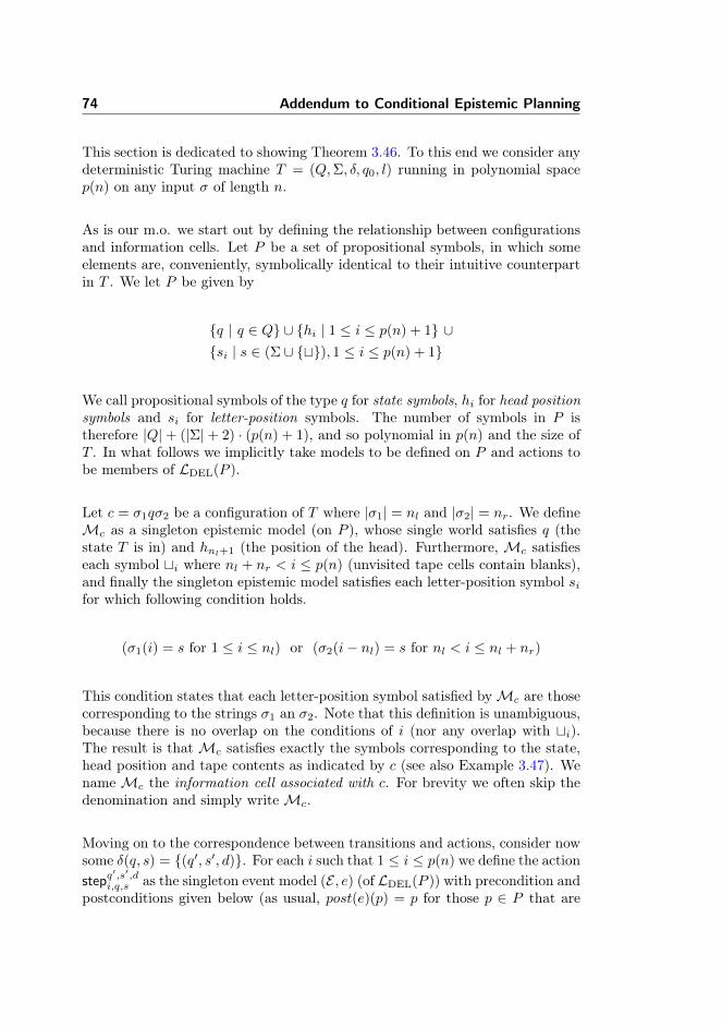
74 Addendum to Conditional Epistemic Planning

This section is dedicated to showing Theorem 3.46. To this end we consider anydeterministic Turing machine T = (Q,Σ, δ, q0, l) running in polynomial spacep(n) on any input σ of length n.

As is our m.o. we start out by defining the relationship between configurationsand information cells. Let P be a set of propositional symbols, in which someelements are, conveniently, symbolically identical to their intuitive counterpartin T . We let P be given by

{q | q ∈ Q} ∪ {hi | 1 ≤ i ≤ p(n) + 1} ∪{si | s ∈ (Σ ∪ {t}), 1 ≤ i ≤ p(n) + 1}

We call propositional symbols of the type q for state symbols, hi for head positionsymbols and si for letter-position symbols. The number of symbols in P istherefore |Q|+ (|Σ|+ 2) · (p(n) + 1), and so polynomial in p(n) and the size ofT . In what follows we implicitly take models to be defined on P and actions tobe members of LDEL(P ).

Let c = σ1qσ2 be a configuration of T where |σ1| = nl and |σ2| = nr. We defineMc as a singleton epistemic model (on P ), whose single world satisfies q (thestate T is in) and hnl+1 (the position of the head). Furthermore, Mc satisfieseach symbol ti where nl + nr < i ≤ p(n) (unvisited tape cells contain blanks),and finally the singleton epistemic model satisfies each letter-position symbol sifor which following condition holds.

(σ1(i) = s for 1 ≤ i ≤ nl) or (σ2(i− nl) = s for nl < i ≤ nl + nr)

This condition states that each letter-position symbol satisfied byMc are thosecorresponding to the strings σ1 an σ2. Note that this definition is unambiguous,because there is no overlap on the conditions of i (nor any overlap with ti).The result is thatMc satisfies exactly the symbols corresponding to the state,head position and tape contents as indicated by c (see also Example 3.47). WenameMc the information cell associated with c. For brevity we often skip thedenomination and simply writeMc.

Moving on to the correspondence between transitions and actions, consider nowsome δ(q, s) = {(q′, s′, d)}. For each i such that 1 ≤ i ≤ p(n) we define the actionstepq

′,s′,di,q,s as the singleton event model (E , e) (of LDEL(P )) with precondition and

postconditions given below (as usual, post(e)(p) = p for those p ∈ P that are

3.4 Simulating Turing Machines 75

not specified).

pre(e) = hi ∧ q ∧ sipost(e)(q) = > if q = q′ post(e)(q) = ⊥ otherwisepost(e)(q′) = >post(e)(si) = > if s = s′ post(e)(si) = ⊥ otherwisepost(e)(s′i) = >post(e)(hi) = ⊥

post(e)(hi−1) = > if d = L post(e)(hi+1) = > otherwise

Effectively, a single transition of T leads to p(n) actions in the planning problemwe construct.

Example 3.47. Figure 3.6 illustrates the relationship between configurationsand information cells, as well as that between transitions and actions. Onthe top left is the configuration c = xyq1z (we omit blanks when specifyingconfigurations). On the bottom left is the singletonMc, and displayed below itis a description of the propositional symbols that it satisfies. In this case we haveq1 is satisfied as this is the state of c, and h3 is satisfied as the machine is readingcell number 3. For each combination of i ∈ {1, . . . , p(n)} and s ∈ (Σ ∪ {t}) wehave a letter-position symbol, meaning that x1, y2, z3,t4, . . . ,tp(n) all belongto P . More generally, we can describe the tape contents for any configuration(as well as describing information cells not corresponding to configurations).

For the Turing machine in this example we use δ(q1, z) = {(q2, z′, R)} meaning

that c yields c′ = xyz′q2. The action simulating this transition is stepq2,z′,R

3,q1,z,

which we have illustrated at the bottom center of Figure 3.6. Here we list theprecondition of the action in the top part. The middle part indicates (using :=)the postconditions of individual propositions, namely those propositions whosetruth value is changed. The lower part contains a subset of these symbols whosetruth value is unchanged. It is clear that this action is applicable inMc. Whatis important here is that the head position 3 is fixed for this action (we definep(n) actions for each transition). As we’re additionally given the letter to beerased from tape (z), as well as the letter that is to be written (z′), we canform the action so that the postcondition of z3 is ⊥ and the postcondition ofz′3 is >. The same applies to the head position symbols, where we’re given thedirection of the transition. For state symbols things are even simpler as theseare modified irrespective of the head position. As the truth value of every otherpropositional symbol is unchanged, the result of the product update is thereforethe information cell associated withMc′ indicated at the bottom right.

Lemma 3.48. Let c = σ1qσ2 be a configuration of T with i = |σ1| + 1 ≤ p(n)being the position of T ’s head, and where c yields c′ due to δ(q, s) = {(q′, s′, d)}.

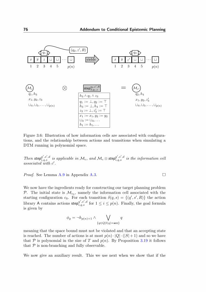
76 Addendum to Conditional Epistemic Planning

x

1

y

2

z

3

q1

t

4

t

5

. . . t

p(n)

(q2, z′, R)

yields x

1

y

2

z′

3

t

4

q2

t

5

. . . t

p(n)

Mc

q1, h3

x1, y2, z3

t4,t5, . . . ,tp(n)

stepq2,z′,R

3,q1,z⊗ =h3 ∧ q1 ∧ z3

q1 := ⊥, q2 := >h3 := ⊥, h4 := >z3 := ⊥, z′3 := >x1 := x1, y2 := y2

t4 := t4, . . .h1 := h1, . . .

Mc′

q2, h4

x1, y2, z′3

t4,t5, . . . ,tp(n)

Figure 3.6: Illustration of how information cells are associated with configura-tions, and the relationship between actions and transitions when simulating aDTM running in polynomial space.

Then stepq′,s′,di,q,s is applicable inMc, andMc ⊗ stepq

′,s′,di,q,s is the information cell

associated with c′.

Proof. See Lemma A.9 in Appendix A.3.

We now have the ingredients ready for constructing our target planning problemP. The initial state is Mc0 , namely the information cell associated with thestarting configuration c0. For each transition δ(q, s) = {(q′, s′, R)} the actionlibrary A contains actions stepq

′,s′,di,q,s for 1 ≤ i ≤ p(n). Finally, the goal formula

is given by

φg = ¬hp(n)+1 ∧∨

{q∈Q|l(q)=acc}

q

meaning that the space bound must not be violated and that an accepting stateis reached. The number of actions is at most p(n) · |Q| · (|S|+ 1) and so we havethat P is polynomial in the size of T and p(n). By Proposition 3.19 it followsthat P is non-branching and fully observable.

We now give an auxiliary result. This we use next when we show that if the

3.4 Simulating Turing Machines 77

starting configuration of T is accepting, then there exists a solution to P; i.e.the “if” part of Theorem 3.46.

Lemma 3.49. Let c = σ1qσ2 be a configuration of T with i = |σ1|+ 1 ≤ p(n),and where c yields c′ due to δ(q, s) = {(q′, s′, d)}. Then Mc |=

rstepq

′,s′,di,q,s

z

sφ

iffMc′ |= φ.

Proof. Using Lemma 3.48 we have that stepq′,s′,di,q,s is applicable in Mc and so

Mc |= 〈stepq′,s′,di,q,s 〉>. Moreover, Mc ⊗ stepq

′,s′,di,q,s is isomorphic to the informa-

tion cell associated with Mc′ . Therefore Mc′ |= φ iff Mc ⊗ stepq′,s′,di,q,s |= φ

iff Mc |= [stepq′,s′,di,q,s ]φ by Lemma 2.16. Recalling Definition 2.11 we conclude

Mc |=rstepq

′,s′,di,q,s

z

sφ iffMc′ |= φ.

Proposition 3.50. If the DTM T accepts σ without violating the space boundp(n), then there exists a solution to the non-branching and fully observable plan-ning P.

Proof. We must show that if c0 is accepting, then there exists a solution to P.We strengthen this and show that if T is in a configuration c = σ1qσ2 whichis x-accepting and |σ1| + 1 ≤ p(n), then there is a plan π s.t. Mc |= JπKs φg,whereMc is the information cell associated with c. As c0 = q0σ is x-acceptingfor some x ∈ N, and the initial state isMc0 , this suffices to prove the result.

We prove this stronger claim by induction on x. If c is 0-accepting then l(q) =acc and the head position is at most p(n) as T does not violate the spacebound. It follows thatMc |= q ∧ ¬hp(n)+1 and thereforeMc |= JskipKs φg thuscompleting the base case. Assume for the induction step that c is (x + 1)-accepting and i ≤ p(n). Then c yields c′ due to some δ(q, s) = {(q′, s′, d)} andc′ is y-accepting for some y ≤ x. To see that the head position of c′ is at mostp(n), we have from T not violating the space bound that if i = p(n) then d = L.From this and c′ being y-accepting we can apply the induction hypothesis andconclude that Mc′ |= JπKs φg for some π. Using Lemma 3.49 it follows thatMc |=

rstepq

′,s′,di,q,s

z

s(JπKs φg), henceMc |=

rstepq

′,s′,di,q,s ;π

z

sφg as required.

We now turn to the “only if” part necessary for Theorem 3.46; i.e. that if asolution exists to P then the starting configuration of T is accepting. To thisend we first show that actions correspond to transitions, that is, if an actionis applicable in some information cell associated with a configuration, then theconfiguration is not halting.

Lemma 3.51. Let c = σ1qσ2 be a configuration of T with i = |σ1| + 1 ≤ p(n)

78 Addendum to Conditional Epistemic Planning

and s = σ2(1). If there is an action E ∈ A s.t. such that Mc |= JEKs φ, thenthere is a successor configuration c′ of c, andMc′ |= φ.

Proof. For the information cell Mc associated with c we have that its singleworld satisfies q, hi and si and no other state, head or letter-position symbols.FromMc |= JEKs φ it follows that E is applicable inMc. There is only a singlecombination in ({1, . . . , p(n)} × Q × S) that defines such an applicable action.As E exists we must have a transition (q′, s′, d) ∈ δ(q, s) and so E = stepq

′,s′,di,q,s .

Therefore c is not halting, and has a successor configuration c′. Using Lemma3.49 andMc |=

rstepq

′,s′,di,q,s

z

sφ, we concludeMc′ |= φ as required.

Proposition 3.52. If there exists a solution to the non-branching and fullyobservable planning problem P, then the DTM T accepts σ without violating thespace bound p(n).

Proof. Assume there exists a π for P s.t. Mc0 |= JπKs φg. We must show thisto imply that c0 = q0σ is an accepting configuration and T does not violate itsspace bound. Letting c = σ1qσ2 be a configuration of T s.t. |σ1|+ 1 ≤ p(n), wewill show the stronger result that if Mc |= JπKs φg, then c is accepting and nofurther computation violates the space bound. We proceed by induction on thelength of π (cf. Theorem 2.25).

For the base case assume |π| = 1, meaning that either π = skip or π = E forsome E ∈ A. The case of Mc |= JskipKs φg means that l(q) = acc, hence c is0-accepting, and as c is a halting configuration no further computation violatesthe space bound. If π = E then we have Mc |= JEKs φg which by Lemma 3.51means that c yields a configuration c′ s.t. Mc′ |= φg. As in the first case thismeans c′ is 0-accepting and halting, hence c is 1-accepting. AsMc′ |= ¬hp(n)+1

the postcondition assigned to hp(n)+1 for E is ⊥. So if |σ1|+ 1 = p(n) then thiscomputation moved the head left, and so the space bound has not been violated.

For the induction step assume thatMc |= JπKs φg and |π| = m+1 form ≥ 1. Noplan has length 0, and so either π = if φ then π1 else π2, or π = π1;π2. We recallthe two claims shown in the proof of Theorem 2.25, stated here equivalently tosuit our needs. First if M |= Jif φ then π1 else π2Ks φg then M |= Jπ1Ks φg orM |= Jπ2Ks φg, with both |π1| ≤ m and |π2| ≤ m (again, no plan has length 0).Second, if |π1;π2| ≥ 2 and M |= Jπ1;π2Ks φg then there exists a plan E ;π′ s.t.M |= JEKs (Jπ′Ks φg) and |π′| ≤ m.

For the case of π = if φ then π1 else π2 we have that Mc |= Jπ1Ks φg with|π1| ≤ m or Mc |= Jπ2Ks φg with |π2| ≤ m. Either way we can immediatelyapply the induction hypothesis, and have that c is accepting and no furthercomputation violates the space bound. In the case where π = π1;π2, there exists

3.4 Simulating Turing Machines 79

a π′ and some E s.t. Mc |= JEKs (Jπ′Ks φg) where |π′| ≤ m. By Lemma 3.51 thismeans that c yields c′ s.t. Mc′ |= Jπ′Ks φg. To show that the computation fromc to c′ does not violate the space bound, consider the case of |σ1|+1 = p(n) andassume towards a contradiction that the postcondition of E assigned to hp(n)+1

is >. From this it follows thatMc′ |= hp(n)+1 and so no action in A is applicable,as actions are not defined for p(n)+1. Consequently π′ is equivalent to skip, butthen follows the falsity Mc′ |= hp(n)+1 ∧ (JskipKs φg), hence the postconditionassigned to hp(n)+1 is ⊥. Therefore the head position in c′ is at most p(n).From this and |π′| ≤ m we can apply the induction hypothesis to conclude thatc′ is x-accepting and no further computation from c′ violates the space bound.Therefore c is (x+ 1)-accepting and no further computation from c violates thespace bound, thereby completing the induction step.

3.4.2 Branching and Fully Observable Problems

Theorem 3.53. The solution existence problem for branching and fully observ-able planning problems is EXP-Complete.

Proof. Hardness is established from Proposition 3.57 and Proposition 3.60 sinceAPSPACE = EXP. Membership follows from Theorem 3.43.

To prove the above we tweak the construction of the previous section, whichallows us to simulate any alternating Turing machine T = (Q,Σ, δ, q0, l) runningin polynomial space p(n) on any input σ of length n. The intuition here is thatwith actions having multiple basic events and where the epistemic relation isthe identity, we can simulate alternation by producing multiple informationcells that correspond to configurations. As a strong solution must work for anyoutcome, this allows us to mimic the behaviour of an ATM in a universal state.The trick of using branching actions for simulating alternation, and the modularmanner in which this can be done is due to [Rintanen, 2004].

We can keep P and the notion of an information cell associated with a configu-ration c as in Section 3.4.1. What we need to change is the actions in the actionlibrary, and when doing so we can even use the actions stepq

′,s′,di,q,s presented

above as building blocks. Recall that an existential configuration is acceptingif some successor configuration is accepting, and that a universal configurationis accepting if every successor configuration is accepting. Therefore our moveto alternating computation requires us to construct actions so that this notionof acceptance is replicated in any solution. For existential configurations wetherefore construct one action for each possible transition, whereas universal

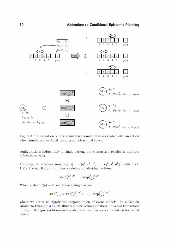
80 Addendum to Conditional Epistemic Planning

x

1

y

2

z

3

q1

t

4

t

5

. . . t

p(n)

(q2, z′, R)

(q3, z′, L)

(q1, x′, R)

yields

x

1

y

2

z′

3

t

4

q2

t

5

. . . t

p(n)

x

1

y

2

q3

z′

3

t

4

t

5

. . . t

p(n)

x

1

y

2

x′

3

t

4

q1

t

5

. . . t

p(n)

Mc

q1, h3

x1, y2, z3

t4,t5, . . . ,tp(n)

stepq3,z′,L

3,q1,z⊗ =

stepq1,x′,R

3,q1,z

]

stepq2,z′,R

3,q1,z

]Mc′2

q3, h2

x1, y2, z′3,t4, . . . ,tp(n)

Mc′1

q2, h4

x1, y2, z′3,t4, . . . ,tp(n)

Mc′3

q1, h4

x1, y2, x′3,t4, . . . ,tp(n)

Figure 3.7: Illustration of how a universal transition is associated with an actionwhen simulating an ATM running in polynomial space.

configurations induce only a single action, but this action results in multipleinformation cells.

Formally, we consider some δ(q, s) = {(q1, s1, d1), . . . , (qk, sk, dk)} with i s.t.1 ≤ i ≤ p(n). If l(q) = ∃, then we define k individual actions

stepq1,s1,d1

i,q,s , . . . , stepqk,sk,dk

i,q,s

When instead l(q) = ∀, we define a single action

step∀i,q,s = stepq1,s1,d1

i,q,s ] · · · ] stepqk,sk,dk

i,q,s

where we use ] to signify the disjoint union of event models. In a fashionsimilar to Example 3.47, we illustrate how actions simulate universal transitionsin Figure 3.7 (preconditions and postconditions of actions are omitted for visualclarity).

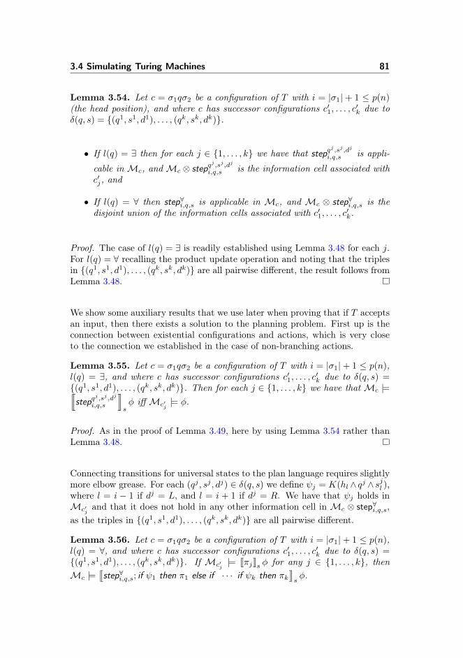
3.4 Simulating Turing Machines 81

Lemma 3.54. Let c = σ1qσ2 be a configuration of T with i = |σ1| + 1 ≤ p(n)(the head position), and where c has successor configurations c′1, . . . , c′k due toδ(q, s) = {(q1, s1, d1), . . . , (qk, sk, dk)}.

• If l(q) = ∃ then for each j ∈ {1, . . . , k} we have that stepqj ,sj ,dj

i,q,s is appli-

cable inMc, andMc ⊗ stepqj ,sj ,dj

i,q,s is the information cell associated withc′j, and

• If l(q) = ∀ then step∀i,q,s is applicable in Mc, and Mc ⊗ step∀i,q,s is thedisjoint union of the information cells associated with c′1, . . . , c′k.

Proof. The case of l(q) = ∃ is readily established using Lemma 3.48 for each j.For l(q) = ∀ recalling the product update operation and noting that the triplesin {(q1, s1, d1), . . . , (qk, sk, dk)} are all pairwise different, the result follows fromLemma 3.48.

We show some auxiliary results that we use later when proving that if T acceptsan input, then there exists a solution to the planning problem. First up is theconnection between existential configurations and actions, which is very closeto the connection we established in the case of non-branching actions.

Lemma 3.55. Let c = σ1qσ2 be a configuration of T with i = |σ1|+ 1 ≤ p(n),l(q) = ∃, and where c has successor configurations c′1, . . . , c′k due to δ(q, s) ={(q1, s1, d1), . . . , (qk, sk, dk)}. Then for each j ∈ {1, . . . , k} we have that Mc |=rstepq

j ,sj ,dj

i,q,s

z

sφ iffMc′j

|= φ.

Proof. As in the proof of Lemma 3.49, here by using Lemma 3.54 rather thanLemma 3.48.

Connecting transitions for universal states to the plan language requires slightlymore elbow grease. For each (qj , sj , dj) ∈ δ(q, s) we define ψj = K(hl ∧ qj ∧ sjl ),where l = i − 1 if dj = L, and l = i + 1 if dj = R. We have that ψj holds inMc′j

and that it does not hold in any other information cell in Mc ⊗ step∀i,q,s,as the triples in {(q1, s1, d1), . . . , (qk, sk, dk)} are all pairwise different.

Lemma 3.56. Let c = σ1qσ2 be a configuration of T with i = |σ1|+ 1 ≤ p(n),l(q) = ∀, and where c has successor configurations c′1, . . . , c′k due to δ(q, s) ={(q1, s1, d1), . . . , (qk, sk, dk)}. If Mc′j

|= JπjKs φ for any j ∈ {1, . . . , k}, thenMc |=

qstep∀i,q,s; if ψ1 then π1 else if · · · if ψk then πk

ysφ.

82 Addendum to Conditional Epistemic Planning

Proof. By construction of ψj we have for any j ∈ {1, . . . , k} that Mc′j|=

((ψ1 → Jπ1Ks φ) ∧ · · · ∧ (ψj → JπjKs φ)) ∧ (ψ1 ∨ · · · ∨ ψk). With this we canuse a derivation like that in the proof of Theorem 2.24 to conclude Mc′j

|=K Jif ψ1 then π1 else if · · · if ψk then πkKs φ (we haveMc′j

|= φ⇔Mc′j|= Kφ

asMc′jis an information cell). Therefore asMc⊗ step∀i,q,s is the disjoint union

of eachMc′1, . . . ,Mc′k

(Lemma 3.54), it follows from Lemma 2.16 that

Mc |=[step∀i,q,s

](K Jif ψ1 then π1 else if · · · if ψk then πkKs φ)

Furthermore step∀i,q,s is applicable since Mc |=∨

1≤j≤k hi ∧ q ∧ si, so Mc |=⟨step∀i,q,s

⟩> and cf. Definition 2.11 we have as required:

Mc |=qstep∀i,q,s; if ψ1 then π1 else if · · · if ψk then πk

ysφ

An important note is that ψj simply shows the existence of a branching formula— it is not a part of the planning problem given below. If such a formula didnot exist the above result could not be established. Constructing our planningproblem P we let the initial stateMc0 and goal formula φg be as in Section 3.4.1.The action library A contains the actions described above for each δ(q, s) ={(q1, s1, d1), . . . , (qk, sk, dk)} subject to l(q). Both P and P are polynomial inthe size of T and p(n), and Proposition 3.20 implies P is branching and fullyobservable.

Proposition 3.57. If the ATM T accepts σ without violating the space boundp(n), then there exists a solution to the branching and fully observable planningP.

Proof. We show that if T is in a configuration c = σ1qσ2 which is x-acceptingand |σ1| + 1 ≤ p(n), then there is a plan π s.t. Mc |= JπKs φg, where Mc isthe information cell associated with c. We proceed by induction on x, withthe base being immediate. Assume for the induction step that c = σ1qσ2 is(x + 1)-accepting, and has successor configurations c′1, . . . , c′k. If l(q) = ∃ thenfor some j ∈ {1, . . . , k} we have that c′j is y-accepting for some y ≤ x. The headposition of c′j is at most p(n) as the computation from c to c′j would otherwisemean T violated the space bound. With this we apply the induction hypothesis,and have that there is a plan πj s.t. Mc′j

|= JπjKs φg. Using Lemma 3.55 it

follows thatMc |=rstepq

j ,sj ,dj

i,q,s

z

s(JπjKs φg), henceMc |=

rstepq

j ,sj ,dj

i,q,s ;πj

z

sφg

as required. If l(q) = ∀ then each c′1, . . . , c′k is y-accepting for some y ≤ x, andthe head position of each such successor configuration is at most p(n). By theinduction hypothesis this means there is a plan πj s.t. Mc′j

|= JπjKs φg for each

3.4 Simulating Turing Machines 83

j ∈ {1, . . . , k}. Using Lemma 3.56 it follows that

Mc |=qstep∀i,q,s; if ψ1 then π1 else if · · · if ψk then πk

ysφg

as required. Assuming that c0 = qσ is an accepting configuration we have thatthere exists a solution to P.

With the first direction of Theorem 3.53 being completed, next up is showingthat existence of a strong solution is a sufficient condition for the starting con-figuration to be accepting. The following two results are analogues to Lemma3.51, now in the context of alternating computation.

Lemma 3.58. Let c = σ1qσ2 be a configuration of T with i = |σ1| + 1 ≤ p(n)and l(q) = ∃. If there is an action E ∈ A such that Mc |= JEKs φ, then c has asuccessor configuration c′, andMc′ |= φ.

Proof. For the information cell Mc associated with c we have that its singleworld satisfies q, hi and si and no other state, head or letter symbols. FromMc |= JEKs φ it follows that E is applicable in Mc. As l(q) = ∃ this meansthat for the combination (i, q, s) we have defined k actions corresponding toδ(q, s) = {(q1, s1, d1), . . . , (qk, sk, dk)}, and these are the only actions applicableinMc. Therefore E = stepq

j ,sj ,dj

i,q,s for some j ∈ {1, . . . , k}, and so c yields c′j . It

follows from Lemma 3.55 andMc |=rstepq

j ,sj ,dj

i,q,s

z

sφ thatMc′j

|= φ.

Lemma 3.59. Let c = σ1qσ2 be a configuration of T with i = |σ1| + 1 ≤ p(n)and l(q) = ∀. If there is an action E ∈ A such that Mc |= JEKs φ, then c hassuccessor configurations c′1, . . . , c′k, andMc′j

|= φ for each j ∈ {1, . . . , k}.

Proof. From the same line of reasoning as in the previous proof we can assumethat some step∀i,q,s is the single applicable action Mc, since l(q) = ∀. FromLemma 3.54 it follows that Mc ⊗ step∀i,q,s is the disjoint union of informationcells associated with c′1, . . . , c′k, and sinceMc⊗ step∀i,q,s |= φ we have by Lemma2.16 thatMc′j

|= φ for each j ∈ {1, . . . , k}.

Proposition 3.60. If there exists a solution to the branching and fully observ-able planning problem P, then the ATM T accepts σ without violating the spacebound p(n).

Proof. Assuming that there exists a solution π for P s.t. Mc0 |= JπKs φg, wemust show that c0 is an accepting configuration and T does not violate its spacebound. Let Mc be the information cell associated with some configurationc = σ1qσ2 of T , with i = |σ1| + 1 and i ≤ p(n). We show the stronger result,

84 Addendum to Conditional Epistemic Planning

that ifMc |= JπKs φg, then c is accepting and no further computation violatesthe space bound. This is by induction on the length of π.

For the base case |π| = 1 and we have either π = skip or π = E for some E ∈ A.If Mc |= JskipKs φg then Mc |= φg, hence l(q) = acc and c is 0-accepting. IfMc |= JEKs φg we have either l(q) = ∃ or l(q) = ∀ as actions are not defined forhalting states. When l(q) = ∃ it follows from Lemma 3.58 that c yields some c′s.t. Mc′ |= φg. Therefore c is 1-accepting as it has a successor configuration c′which is 0-accepting. When l(q) = ∀ we apply Lemma 3.59 and have that c hassuccessor configurations c′1, . . . , c′k s.t. Mc′j

|= φg for j ∈ {1, . . . , k}. Thereforeeach c′j is 0-accepting and hence c is 1-accepting. As in the proof of Proposition3.52, any information cell satisfying φg cannot satisfy hp(n)+1, and so the spacebound of T is not violated.

For the induction step assume that |π| = m+ 1. As in the proof of Proposition3.52 we have for π = if φ then π1 else π2 thatMc |= Jπ1Ks φg for |π1| ≤ m or thatMc |= Jπ2Ks φg for |π2| ≤ m, so applying the induction hypothesis immediatelygives that c is accepting and no further computation violates the space bound.Moreover, for π = π1;π2 we may assumeMc |= JEKs (Jπ′Ks φg) where |π′| ≤ m.If l(q) = ∃ it follows from Lemma 3.58 that c has some successor configurationc′ with Mc′ |= Jπ′Ks φg. As |π′| ≤ m we can apply the induction hypothesisto conclude that c′ is x-accepting for x ∈ N and thus c is (x + 1)-accepting.When l(q) = ∀ we have from Lemma 3.59 that c has successor configurationsc′1, . . . , c

′k s.t. Mc′j

|= Jπ′Ks φg for each j ∈ {1, . . . , k}. As |π′| ≤ m we can applythe induction hypothesis and have that each c′j is xj-accepting for some xj ∈ N,hence c is (xmax + 1)-accepting where xmax = max(x1, . . . , xk).

Showing that no further computation from c violates the space bound is forl(q) = ∃ exactly as in the proof of Proposition 3.52, viz. using proof by con-tradiction. The same applies to l(q) = ∀, where by assuming that the headposition of any c′j is such that Mc′j

|= hp(n)+1 we derive the contradictionMc′j

|= hp(n)+1 ∧ (JskipKs φg).

3.4.3 Non-branching and Partially Observable Problems

Next up are planning problems with partial observability, and for this we turnto Turing machines running in exponential space. As noted previously, when welater make the move from DTMs to ATMs, we can reuse the above approach forsimulating alternation. First up however, is showing how configurations withexponentially many letters on the tape can be represented.

3.4 Simulating Turing Machines 85

We let T = (Q,Σ, δ, q0, l) be a deterministic Turing machine running in expo-nential space e(n) on any input σ of length n. Adding partial observabilityallows us to use actions whose epistemic relation is not the identity. In fact weonly need such actions for some initial steps; actions for simulating transitionsare still singletons. In effect we now have non-singleton information cells atour disposal, and this allows us to encode an entire configuration, including theexponentially in n sized tape, as a single information cell. In the presentationthat follows, we do not rely on the notions developed in Section 3.4.1 and Sec-tion 3.4.2, even though we for convenience use some overlapping notation. Theresult we’re after first is this.

Theorem 3.61. The solution existence problem for non-branching and partiallyobservable planning problems is EXPSPACE-Complete.

Proof. Hardness follows from Proposition 3.66 and Proposition 3.67. Member-ship follows from Theorem 3.44.

We’ll be using two ideas that we credit [Rintanen, 2004]. First is the use ofpropositional symbols as bit encodings of the head position, and further givingeach world a distinct identifier, which allows succinct actions to faithfully sim-ulate transitions (Rintanen does not use an identifier per say, rather he keepstrack of a watched tape cell randomly chosen at the start of plan execution).Here our construction is very similar. Second is the use of partial observabil-ity to represent exponentially many possibilities. Here our construction differs,because our model of observation is unlike that of [Rintanen, 2004], and so wedo not have the option of succinctly specifying an initial state that contains ex-ponentially many possibilities. We overcome this by employing a bootstrappingprocedure.

The first component of the simulation is to show how configurations and infor-mation cells correspond. We will use b = dlog2(e(n) + 1)e, which is enough bitsto represent any integer between 1 and e(n) + 1. Note that b is polynomial inn. We let P be the following set of symbols.

{q | q ∈ Q} ∪ {s | s ∈ (Σ ∪ {t})} ∪{hi | 1 ≤ i ≤ b} ∪ {idi | 1 ≤ i ≤ b} ∪{initi | 0 ≤ i ≤ b}

We say that propositional symbols of the type q is a state symbol, s is a lettersymbol, hi is a head position bit, idi is an identification bit and initi is aninitialization control symbol (we purposely introduce more control symbols thanwe do bits).

The first thing to note is that unlike the case of polynomial space TMs, we

86 Addendum to Conditional Epistemic Planning

do not form letter-position symbols for representing tape contents. Instead, wewill be giving each world in an information cell a unique identifier (the role ofidentification bits), which represents its position on tape. Moreover, we alsoencode the current position of the head using the head position bits, whichchanges as the head moves. We use initi for bootstrapping the initial state ofthe planning problem, a procedure which we return to later. For conveniencewe write h to indicate the integer represented by h1, . . . , hb and similarly withid for id1, . . . idb. Moreover, for any integer j between 1 and 2b, we use j1, . . . , jbto denote its bit (0’s and 1’s) representation.

We’ll now formally show what the information cells we’re after look like (seealso Figure 3.8). Consider a configuration c = σ1qσ2 of T where |σ1| = nl and|σ2| = nr. We define Mc = (W,∼, V ) on P as the information cell associatedwith c. Here W = {wj | 1 ≤ j ≤ 2b} and ∼ is (by definition) the universalrelation onW ; i.e. our information cells contain 2b worlds. We give the valuationV so that state symbols and head identification bits have the same truth valuein every world, as these are global properties of c. Further, each world is givena distinct id to indicate a cell index as well as the symbol corresponding to theletter at this particular cell index. For each world wj ∈W this means:

wj ∈ V (idi) if ji is 1 j is interpreted as an integerwj ∈ V (hi) if (nl + 1)i is 1 nl + 1 is the position of the headV (q) = W

V (q′) = ∅ for q′ ∈ (Q \ {q})

wj ∈ V (s) if

j ≤ nl and σ1(j) = s

j > nl, j ≤ nl + nr and σ2(j − nl) = s

j > nl + nr, j ≤ e(n) + 1 and s = tfor s ∈ (Σ ∪ {t})

V (initb) = W

The three cases for wj ∈ V (s) imply that wj is at most in one valuation ofs ∈ (Σ∪{t}), and that if j > e(n) + 1 we associate it with no symbol. We havedefined Mc so that it contains least one more world than there are tape cells,which means that space bound violation is well-defined (detection follows fromthe goal formula). As a technical quirk V (initb) = W is used to indicate thatbootstrapping has taken place.

Example 3.62. We illustrate an information cell associated with some config-uration c = σ1qσ2 of T in Figure 3.8. We’ll let |σ1| + 1 = m be the positionof the head, and assume σ2(1) = x is currently read. This meansMc containsa world wm whose id and h bit encodings are both equal to m. In accordancewith the discussion below this example, we simply write id = m and h = m toindicate this. Also, wm satisfies the state symbol q as well as initb, and finallyit satisfies x. Say that x is also written on the cell of some other position o.

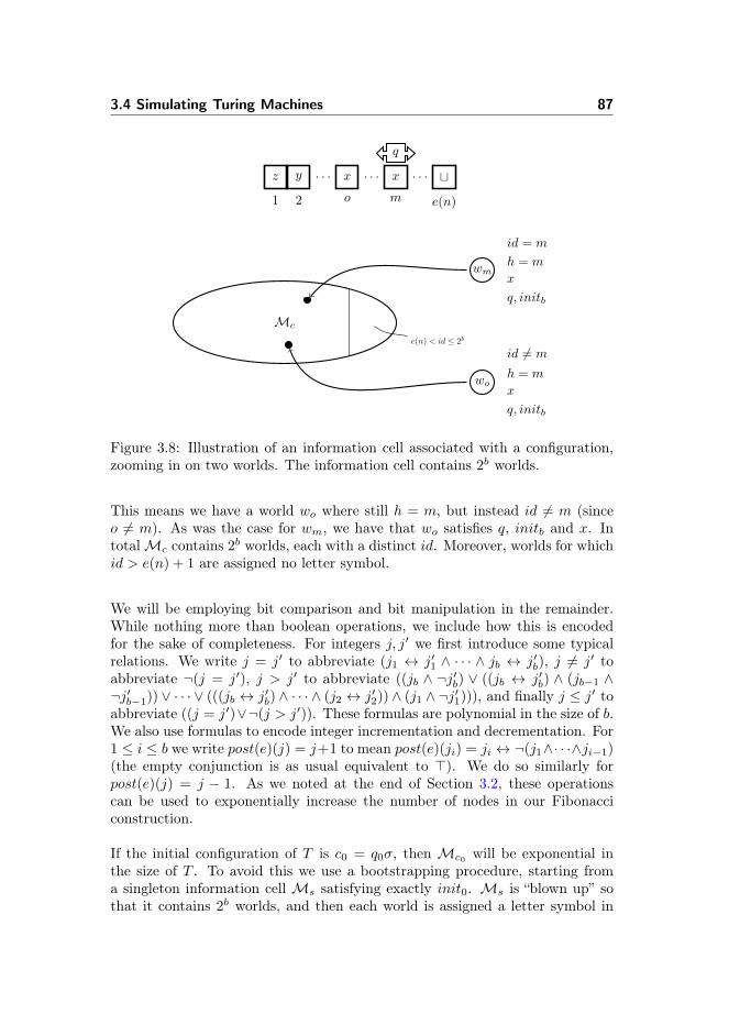
3.4 Simulating Turing Machines 87

z

1

y

2

. . . x

o

. . . x

m

q

. . . t

e(n)

Mc

wm

id = m

h = m

x

q, initb

wo

id 6= m

h = m

x

q, initb

e(n) < id ≤ 2b

Figure 3.8: Illustration of an information cell associated with a configuration,zooming in on two worlds. The information cell contains 2b worlds.

This means we have a world wo where still h = m, but instead id 6= m (sinceo 6= m). As was the case for wm, we have that wo satisfies q, initb and x. IntotalMc contains 2b worlds, each with a distinct id. Moreover, worlds for whichid > e(n) + 1 are assigned no letter symbol.

We will be employing bit comparison and bit manipulation in the remainder.While nothing more than boolean operations, we include how this is encodedfor the sake of completeness. For integers j, j′ we first introduce some typicalrelations. We write j = j′ to abbreviate (j1 ↔ j′1 ∧ · · · ∧ jb ↔ j′b), j 6= j′ toabbreviate ¬(j = j′), j > j′ to abbreviate ((jb ∧ ¬j′b) ∨ ((jb ↔ j′b) ∧ (jb−1 ∧¬j′b−1)) ∨ · · · ∨ (((jb ↔ j′b) ∧ · · · ∧ (j2 ↔ j′2)) ∧ (j1 ∧ ¬j′1))), and finally j ≤ j′ toabbreviate ((j = j′)∨¬(j > j′)). These formulas are polynomial in the size of b.We also use formulas to encode integer incrementation and decrementation. For1 ≤ i ≤ b we write post(e)(j) = j+1 to mean post(e)(ji) = ji ↔ ¬(j1∧· · ·∧ji−1)(the empty conjunction is as usual equivalent to >). We do so similarly forpost(e)(j) = j − 1. As we noted at the end of Section 3.2, these operationscan be used to exponentially increase the number of nodes in our Fibonacciconstruction.

If the initial configuration of T is c0 = q0σ, then Mc0 will be exponential inthe size of T . To avoid this we use a bootstrapping procedure, starting froma singleton information cell Ms satisfying exactly init0. Ms is “blown up” sothat it contains 2b worlds, and then each world is assigned a letter symbol in

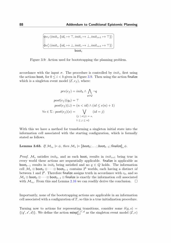
88 Addendum to Conditional Epistemic Planning

ei:〈initi, {idi 7→ >, initi 7→ ⊥, initi+1 7→ >}〉

e′i:〈initi, {idi 7→ ⊥, initi 7→ ⊥, initi+1 7→ >}〉booti

Figure 3.9: Action used for bootstrapping the planning problem.

accordance with the input σ. The procedure is controlled by initi, first usingthe actions booti for 0 ≤ i < b given in Figure 3.9. Then using the action finalizewhich is a singleton event model (E , ef ), where:

pre(ef ) = initb ∧∧q∈Q¬q

post(ef )(q0) = >post(ef )(t) = (n < id) ∧ (id ≤ e(n) + 1)

∀s ∈ Σ : post(ef )(s) =∨

{j | σ(j) = s,

1 ≤ j ≤ n}

(id = j)

With this we have a method for transforming a singleton initial state into theinformation cell associated with the starting configuration, which is formallystated as follows.

Lemma 3.63. IfMc0 |= φ, thenMs |= Jboot0; . . . ; bootb−1; finalizeKs φ.

Proof. Ms satisfies init0, and as each booti results in initi+1 being true inevery world these actions are sequentially applicable. finalize is applicable asbootb−1 results in initb being satisfied and no q ∈ Q holds. The informationcell Ms ⊗ boot0 ⊗ · · · ⊗ bootb−1 contains 2b worlds, each having a distinct idbetween 1 and 2b. Therefore finalize assigns truth in accordance with c0, and soMs ⊗ boot0 ⊗ · · · ⊗ bootb−1 ⊗ finalize is exactly the information cell associatedwithMc0 . From this and Lemma 2.16 we can readily derive the conclusion.

Importantly, none of the bootstrapping actions are applicable in an informationcell associated with a configuration of T , so this is a true initialization procedure.

Turning now to actions for representing transitions, consider some δ(q, s) ={(q′, s′, d)}. We define the action estepq

′,s′,dq,s as the singleton event model (E , e)

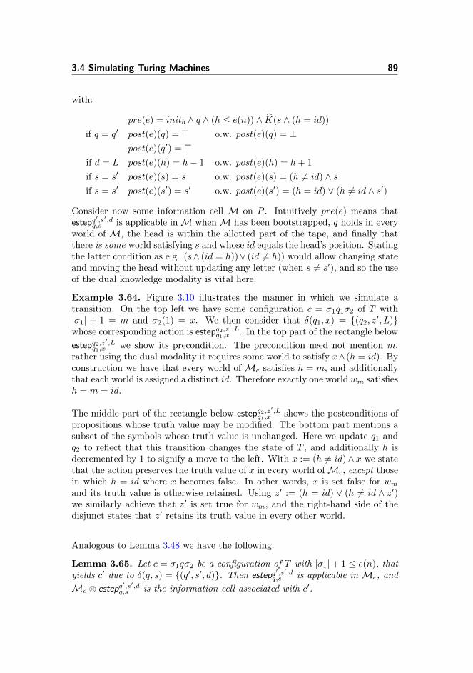
3.4 Simulating Turing Machines 89

with:

pre(e) = initb ∧ q ∧ (h ≤ e(n)) ∧ K̂(s ∧ (h = id))

if q = q′ post(e)(q) = > o.w. post(e)(q) = ⊥post(e)(q′) = >

if d = L post(e)(h) = h− 1 o.w. post(e)(h) = h+ 1

if s = s′ post(e)(s) = s o.w. post(e)(s) = (h 6= id) ∧ sif s = s′ post(e)(s′) = s′ o.w. post(e)(s′) = (h = id) ∨ (h 6= id ∧ s′)

Consider now some information cell M on P . Intuitively pre(e) means thatestepq

′,s′,dq,s is applicable inM whenM has been bootstrapped, q holds in every

world of M, the head is within the allotted part of the tape, and finally thatthere is some world satisfying s and whose id equals the head’s position. Statingthe latter condition as e.g. (s∧ (id = h))∨ (id 6= h)) would allow changing stateand moving the head without updating any letter (when s 6= s′), and so the useof the dual knowledge modality is vital here.

Example 3.64. Figure 3.10 illustrates the manner in which we simulate atransition. On the top left we have some configuration c = σ1q1σ2 of T with|σ1| + 1 = m and σ2(1) = x. We then consider that δ(q1, x) = {(q2, z

′, L)}whose corresponding action is estepq2,z

′,Lq1,x . In the top part of the rectangle below

estepq2,z′,L

q1,x we show its precondition. The precondition need not mention m,rather using the dual modality it requires some world to satisfy x∧ (h = id). Byconstruction we have that every world ofMc satisfies h = m, and additionallythat each world is assigned a distinct id. Therefore exactly one world wm satisfiesh = m = id.

The middle part of the rectangle below estepq2,z′,L

q1,x shows the postconditions ofpropositions whose truth value may be modified. The bottom part mentions asubset of the symbols whose truth value is unchanged. Here we update q1 andq2 to reflect that this transition changes the state of T , and additionally h isdecremented by 1 to signify a move to the left. With x := (h 6= id)∧ x we statethat the action preserves the truth value of x in every world ofMc, except thosein which h = id where x becomes false. In other words, x is set false for wmand its truth value is otherwise retained. Using z′ := (h = id) ∨ (h 6= id ∧ z′)we similarly achieve that z′ is set true for wm, and the right-hand side of thedisjunct states that z′ retains its truth value in every other world.

Analogous to Lemma 3.48 we have the following.

Lemma 3.65. Let c = σ1qσ2 be a configuration of T with |σ1|+ 1 ≤ e(n), thatyields c′ due to δ(q, s) = {(q′, s′, d)}. Then estepq

′,s′,dq,s is applicable in Mc, and

Mc ⊗ estepq′,s′,dq,s is the information cell associated with c′.

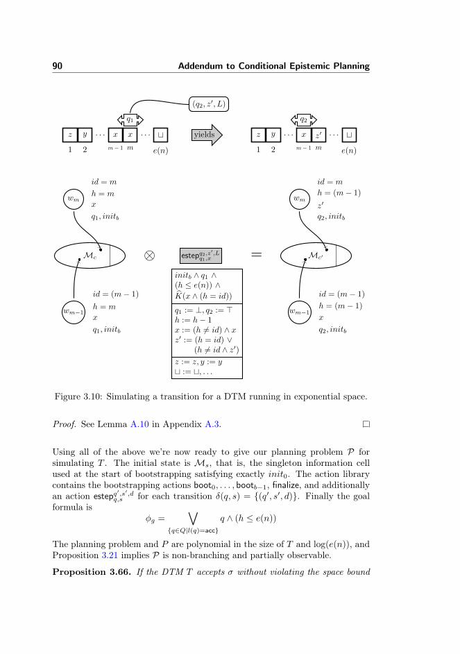
90 Addendum to Conditional Epistemic Planning

z

1

y

2

. . . x

m− 1

x

m

q1

. . . t

e(n)

(q2, z′, L)

yields z

1

y

2

. . . x

m− 1

q2

z′

m

. . . t

e(n)

Mc

wm

id = m

h = m

x

q1, initb

wm−1

id = (m− 1)

h = m

x

q1, initb

estepq2,z′,L

q1,x⊗ =

initb ∧ q1 ∧(h ≤ e(n)) ∧K̂(x ∧ (h = id))

q1 := ⊥, q2 := >h := h− 1x := (h 6= id) ∧ xz′ := (h = id) ∨

(h 6= id ∧ z′)z := z, y := yt := t, . . .

Mc′

wm

id = m

h = (m− 1)

z′

q2, initb

wm−1

id = (m− 1)

h = (m− 1)

x

q2, initb

Figure 3.10: Simulating a transition for a DTM running in exponential space.

Proof. See Lemma A.10 in Appendix A.3.

Using all of the above we’re now ready to give our planning problem P forsimulating T . The initial state is Ms, that is, the singleton information cellused at the start of bootstrapping satisfying exactly init0. The action librarycontains the bootstrapping actions boot0, . . . , bootb−1, finalize, and additionallyan action estepq

′,s′,dq,s for each transition δ(q, s) = {(q′, s′, d)}. Finally the goal

formula isφg =

∨{q∈Q|l(q)=acc}

q ∧ (h ≤ e(n))

The planning problem and P are polynomial in the size of T and log(e(n)), andProposition 3.21 implies P is non-branching and partially observable.

Proposition 3.66. If the DTM T accepts σ without violating the space bound

3.4 Simulating Turing Machines 91

e(n), then there exists a solution to the non-branching and partially observableplanning problem P.

Proof. The proof is along the lines of that used when T runs in polynomialspace, namely by induction x, showing that for any configuration c that is x-accepting, there exists a strong solution forMc. The addition here is the use ofLemma 3.63 for additionally showing that any such plan can be prefixed withboot0; . . . ; bootb−1; finalize to work from the initial stateMc. The result is fullyshown in the proof of Lemma A.12 in Appendix A.3.

For the other direction of Theorem 3.61 we have the following.

Proposition 3.67. If there exists a solution to the non-branching and partiallyobservable planning problem P, then the DTM T accepts σ without violating thespace bound e(n).

Proof. First we can show that the bootstrapping procedure must always takeplace in a strong solution to P. Following this we proceed along the lines of theproof of Proposition 3.52, that is, by induction on the length of a solution forany information cell associated with a configuration. Again the goal formulaensures the space bound of T is not violated if there exists a solution to P, andfurther that c0 is an accepting configuration. For a full proof see Lemma A.14in Appendix A.3.

3.4.4 Branching and Partially Observable Problems

Last on our agenda in the following result.

Theorem 3.68. The solution existence problem for branching and partiallyobservable planning problems is 2EXP-Complete.

Proof. Hardness is established from Proposition 3.70 and Proposition 3.71 sinceAEXPSPACE = 2EXP. Membership follows from Theorem 3.42.

We can augment the constructions of the previous section so that alternatingcomputation can be simulated. Doing so is decidedly close to the techniques ofSection 3.4.2, where we lifted DTMs with a polynomial space bound to ATMswith same bound. Therefore we shall only briefly describe the construction, andplace full proofs in the appendix.

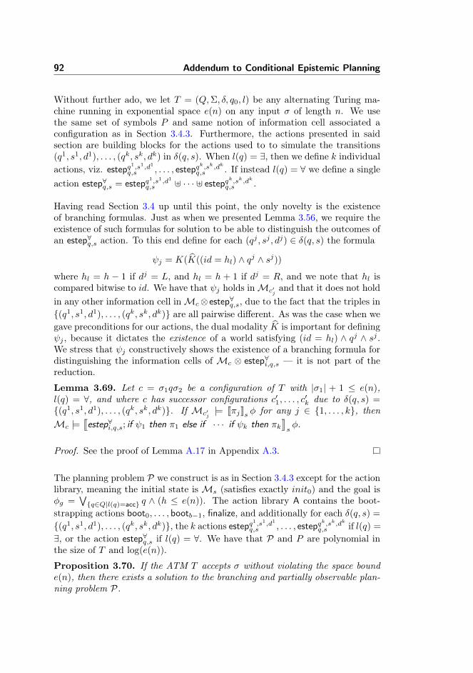
92 Addendum to Conditional Epistemic Planning

Without further ado, we let T = (Q,Σ, δ, q0, l) be any alternating Turing ma-chine running in exponential space e(n) on any input σ of length n. We usethe same set of symbols P and same notion of information cell associated aconfiguration as in Section 3.4.3. Furthermore, the actions presented in saidsection are building blocks for the actions used to to simulate the transitions(q1, s1, d1), . . . , (qk, sk, dk) in δ(q, s). When l(q) = ∃, then we define k individualactions, viz. estepq

1,s1,d1

q,s , . . . , estepqk,sk,dk

q,s . If instead l(q) = ∀ we define a singleaction estep∀q,s = estepq

1,s1,d1

q,s ] · · · ] estepqk,sk,dk

q,s .

Having read Section 3.4 up until this point, the only novelty is the existenceof branching formulas. Just as when we presented Lemma 3.56, we require theexistence of such formulas for solution to be able to distinguish the outcomes ofan estep∀q,s action. To this end define for each (qj , sj , dj) ∈ δ(q, s) the formula

ψj = K(K̂((id = hl) ∧ qj ∧ sj))

where hl = h − 1 if dj = L, and hl = h + 1 if dj = R, and we note that hl iscompared bitwise to id. We have that ψj holds inMc′j

and that it does not holdin any other information cell inMc⊗ estep∀q,s, due to the fact that the triples in{(q1, s1, d1), . . . , (qk, sk, dk)} are all pairwise different. As was the case when wegave preconditions for our actions, the dual modality K̂ is important for definingψj , because it dictates the existence of a world satisfying (id = hl) ∧ qj ∧ sj .We stress that ψj constructively shows the existence of a branching formula fordistinguishing the information cells of Mc ⊗ estep∀i,q,s — it is not part of thereduction.

Lemma 3.69. Let c = σ1qσ2 be a configuration of T with |σ1| + 1 ≤ e(n),l(q) = ∀, and where c has successor configurations c′1, . . . , c′k due to δ(q, s) ={(q1, s1, d1), . . . , (qk, sk, dk)}. If Mc′j

|= JπjKs φ for any j ∈ {1, . . . , k}, thenMc |=

qestep∀i,q,s; if ψ1 then π1 else if · · · if ψk then πk

ysφ.

Proof. See the proof of Lemma A.17 in Appendix A.3.

The planning problem P we construct is as in Section 3.4.3 except for the actionlibrary, meaning the initial state isMs (satisfies exactly init0) and the goal isφg =

∨{q∈Q|l(q)=acc} q ∧ (h ≤ e(n)). The action library A contains the boot-

strapping actions boot0, . . . , bootb−1, finalize, and additionally for each δ(q, s) =

{(q1, s1, d1), . . . , (qk, sk, dk)}, the k actions estepq1,s1,d1q,s , . . . , estepqk,sk,dk

q,s if l(q) =

∃, or the action estep∀q,s if l(q) = ∀. We have that P and P are polynomial inthe size of T and log(e(n)).

Proposition 3.70. If the ATM T accepts σ without violating the space bounde(n), then there exists a solution to the branching and partially observable plan-ning problem P.

3.5 Conclusion and Discussion 93

Proof. See the proof of Lemma A.18 in Appendix A.3.

Proposition 3.71. If there exists a solution to the branching and partiallyobservable planning problem P, then the ATM T accepts σ without violating thespace bound e(n).

Proof. See the proof of Lemma A.21 in Appendix A.3.

3.5 Conclusion and Discussion

In this chapter we took at closer look at the computational complexity of condi-tional epistemic planning as propagated in Chapter 2, namely by investigatingthe decision problem of whether a strong solution exists to a planning problem.Our first step was to illustrate that using the StrongPlan algorithm for thispurpose was infeasible. We then took the natural step and introduced planninggraphs as an alternative to planning trees, subsequently showing that the notionof a solved planning tree corresponds to that of a solved planning graph. Ourresults were with regards to four types of planning problems, separated by thelevel of observability (partial or full) and whether or not actions were branching.We gave the procedure SolutionExists for optimally deciding the solution ex-istence problem in the case of branching planning problems. For non-branchingplanning problems, where a solution can always be found that is sequential, wecould improve the upper bound of the corresponding solution existence problem.Having shown membership, we proceeded to construct epistemic planning prob-lems that simulated Turing machines, and used this to show that each of thefour variants of the solution existence problem were complete for their respectivecomplexity class. The results are summarized in Figure 3.11, and we note thatalong the way we used insights that must be credited [Bylander, 1994, Rintanen,2004].

We now return to the two prudent questions mentioned at the beginning ofSection 3.4. Our sincere answer as to why we have not presented a reductionfrom the plan existence problem of [Rintanen, 2004] to our solution existenceproblem here is simply that we have not been able to find one that works in thegeneral case. Because the complexity classes we deal with are all closed underpolynomial-time reductions, we have however established that a reduction existin both directions. The two reductions that would be interesting and naturalwould allow for transforming operators (as given in [Rintanen, 2004, Definition2]) to event models and event models to operators.

From operators to event models the issue is that an operator may be very

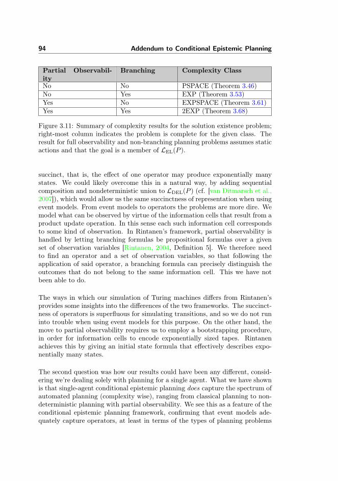
94 Addendum to Conditional Epistemic Planning

Partial Observabil-ity

Branching Complexity Class

No No PSPACE (Theorem 3.46)No Yes EXP (Theorem 3.53)Yes No EXPSPACE (Theorem 3.61)Yes Yes 2EXP (Theorem 3.68)

Figure 3.11: Summary of complexity results for the solution existence problem;right-most column indicates the problem is complete for the given class. Theresult for full observability and non-branching planning problems assumes staticactions and that the goal is a member of LEL(P ).

succinct, that is, the effect of one operator may produce exponentially manystates. We could likely overcome this in a natural way, by adding sequentialcomposition and nondeterministic union to LDEL(P ) (cf. [van Ditmarsch et al.,2007]), which would allow us the same succinctness of representation when usingevent models. From event models to operators the problems are more dire. Wemodel what can be observed by virtue of the information cells that result from aproduct update operation. In this sense each such information cell correspondsto some kind of observation. In Rintanen’s framework, partial observability ishandled by letting branching formulas be propositional formulas over a givenset of observation variables [Rintanen, 2004, Definition 5]. We therefore needto find an operator and a set of observation variables, so that following theapplication of said operator, a branching formula can precisely distinguish theoutcomes that do not belong to the same information cell. This we have notbeen able to do.

The ways in which our simulation of Turing machines differs from Rintanen’sprovides some insights into the differences of the two frameworks. The succinct-ness of operators is superfluous for simulating transitions, and so we do not runinto trouble when using event models for this purpose. On the other hand, themove to partial observability requires us to employ a bootstrapping procedure,in order for information cells to encode exponentially sized tapes. Rintanenachieves this by giving an initial state formula that effectively describes expo-nentially many states.

The second question was how our results could have been any different, consid-ering we’re dealing solely with planning for a single agent. What we have shownis that single-agent conditional epistemic planning does capture the spectrum ofautomated planning (complexity wise), ranging from classical planning to non-deterministic planning with partial observability. We see this as a feature of theconditional epistemic planning framework, confirming that event models ade-quately capture operators, at least in terms of the types of planning problems

3.5 Conclusion and Discussion 95

they can describe (cf. discussion of succinctness above). That this need not bethe case is exemplified in the “KBPs as Plans” approach of [Lang and Zanuttini,2013]. Here an action cannot be both fully observable and branching, meaningthat the class of planning problems that are EXP-Complete is not captured.

Using the results in this chapter we can conclude that, for better or for worse,the computational complexity associated with conditional epistemic planningcoincides with the results known from automated planning. In terms of asymp-totic complexity, we need not be put off by our framework and surrender to theMarkovian route usually taken in automated planning. From a methodologicalperspective we have illustrated that epistemic model theory is crucial in devel-oping optimal decision procedures for the solution existence problem. Whilethe results from epistemic model theory that we have used are not particularlysophisticated, they provide us with just what we need. We can keep the size ofan information cell down by computing its bisimulation contraction, and we canput an upper bound on the number of distinct information cells we may reach.In going beyond single-agent epistemic planning, notions from model theory arelikely to play an equally important role. Incidentally, it is exactly the modeltheory of epistemic-plausibility models that we take to investigate in the ensuingchapter.

96 Addendum to Conditional Epistemic Planning

Chapter 4

Bisimulation for single-agentplausibility models

This chapter is a replicate of [Andersen et al., 2013] which appers in the pro-ceedings of the 26th Australasian Conference on Artificial Intelligence, 2013, inOtago, New Zealand. In the following presentation a few minor corrections havebeen made.

98 Bisimulation for single-agent plausibility models

Bisimulation for single-agent plausibility models

Mikkel Birkegaard Andersen∗ Thomas Bolander∗

Hans van Ditmarsch† Martin Holm Jensen∗∗DTU Compute, Technical University of Denmark

†LORIA, CNRS, Université de Lorraine

Abstract

Epistemic plausibility models are Kripke models agents use to rea-son about the knowledge and beliefs of themselves and each other.Restricting ourselves to the single-agent case, we determine whensuch models are indistinguishable in the logical language containingconditional belief, i.e., we define a proper notion of bisimulation, andprove that bisimulation corresponds to logical equivalence on image-finite models. We relate our results to other epistemic notions, suchas safe belief and degrees of belief. Our results imply that there areonly finitely many non-bisimilar single-agent epistemic plausibilitymodels on a finite set of propositions. This gives decidability forsingle-agent epistemic plausibility planning.

4.1 Introduction

A typical approach in belief revision involves preferential orders to express de-grees of belief and knowledge [Kraus et al., 1990, Meyer et al., 2000]. This goesback to the ‘systems of spheres’ in [Lewis, 1973, Grove, 1988]. Dynamic doxas-tic logic was proposed and investigated in [Segerberg, 1998] in order to providea link between the (non-modal logical) belief revision and modal logics with

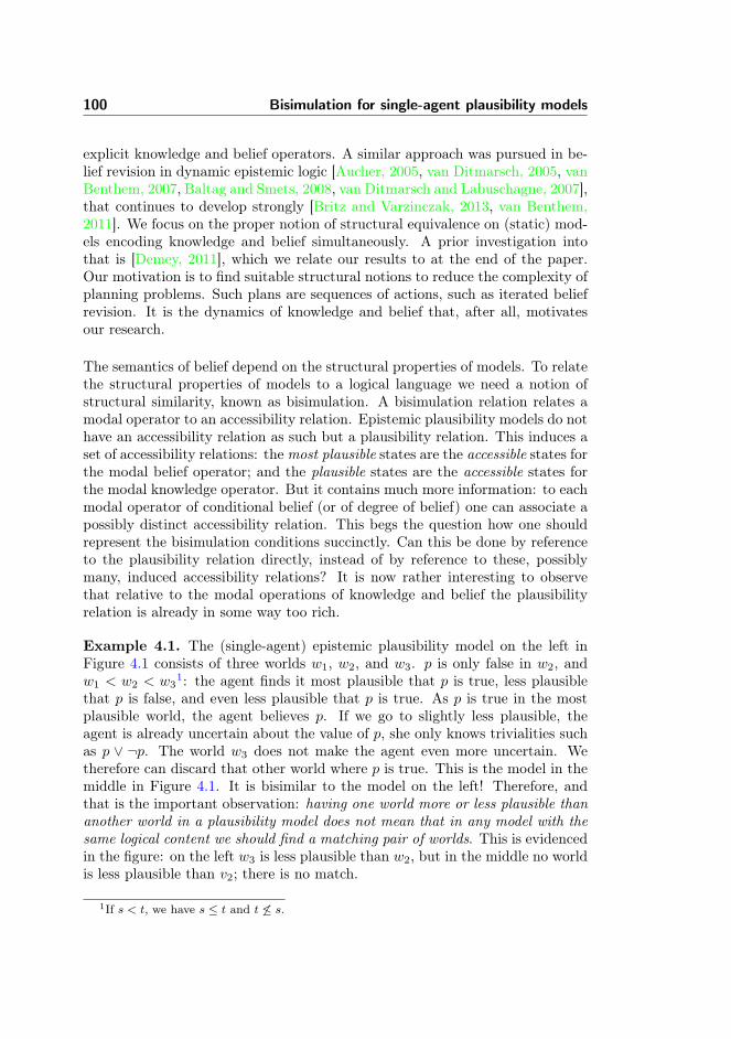
100 Bisimulation for single-agent plausibility models

explicit knowledge and belief operators. A similar approach was pursued in be-lief revision in dynamic epistemic logic [Aucher, 2005, van Ditmarsch, 2005, vanBenthem, 2007, Baltag and Smets, 2008, van Ditmarsch and Labuschagne, 2007],that continues to develop strongly [Britz and Varzinczak, 2013, van Benthem,2011]. We focus on the proper notion of structural equivalence on (static) mod-els encoding knowledge and belief simultaneously. A prior investigation intothat is [Demey, 2011], which we relate our results to at the end of the paper.Our motivation is to find suitable structural notions to reduce the complexity ofplanning problems. Such plans are sequences of actions, such as iterated beliefrevision. It is the dynamics of knowledge and belief that, after all, motivatesour research.

The semantics of belief depend on the structural properties of models. To relatethe structural properties of models to a logical language we need a notion ofstructural similarity, known as bisimulation. A bisimulation relation relates amodal operator to an accessibility relation. Epistemic plausibility models do nothave an accessibility relation as such but a plausibility relation. This induces aset of accessibility relations: themost plausible states are the accessible states forthe modal belief operator; and the plausible states are the accessible states forthe modal knowledge operator. But it contains much more information: to eachmodal operator of conditional belief (or of degree of belief) one can associate apossibly distinct accessibility relation. This begs the question how one shouldrepresent the bisimulation conditions succinctly. Can this be done by referenceto the plausibility relation directly, instead of by reference to these, possiblymany, induced accessibility relations? It is now rather interesting to observethat relative to the modal operations of knowledge and belief the plausibilityrelation is already in some way too rich.

Example 4.1. The (single-agent) epistemic plausibility model on the left inFigure 4.1 consists of three worlds w1, w2, and w3. p is only false in w2, andw1 < w2 < w3

1: the agent finds it most plausible that p is true, less plausiblethat p is false, and even less plausible that p is true. As p is true in the mostplausible world, the agent believes p. If we go to slightly less plausible, theagent is already uncertain about the value of p, she only knows trivialities suchas p ∨ ¬p. The world w3 does not make the agent even more uncertain. Wetherefore can discard that other world where p is true. This is the model in themiddle in Figure 4.1. It is bisimilar to the model on the left! Therefore, andthat is the important observation: having one world more or less plausible thananother world in a plausibility model does not mean that in any model with thesame logical content we should find a matching pair of worlds. This is evidencedin the figure: on the left w3 is less plausible than w2, but in the middle no worldis less plausible than v2; there is no match.

1If s < t, we have s ≤ t and t 6≤ s.

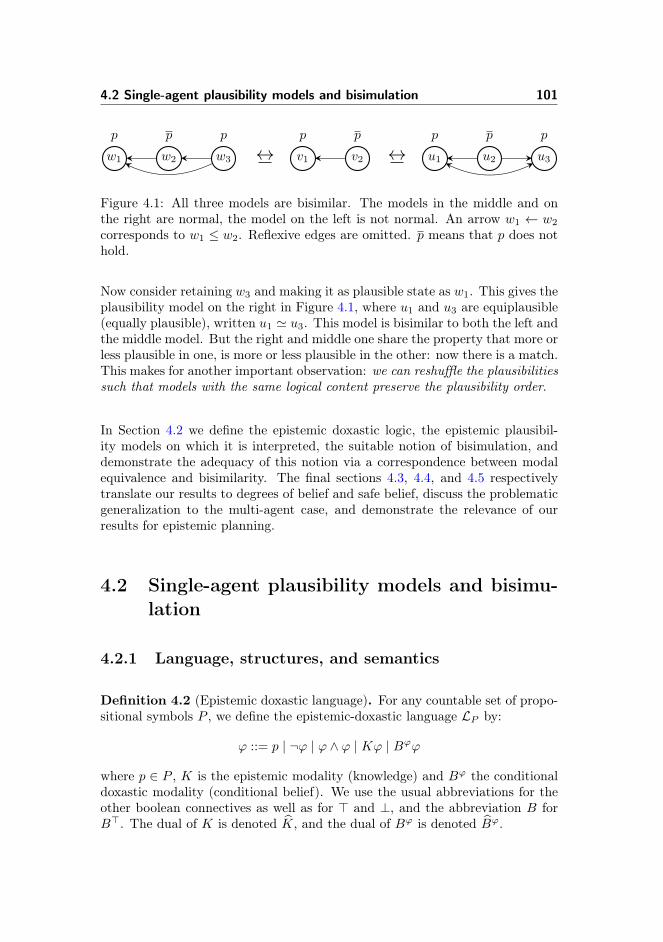
4.2 Single-agent plausibility models and bisimulation 101

w1

p

w2

p

w3

p

↔ v1

p

v2

p

↔ u1

p

u2

p

u3

p

Figure 4.1: All three models are bisimilar. The models in the middle and onthe right are normal, the model on the left is not normal. An arrow w1 ← w2

corresponds to w1 ≤ w2. Reflexive edges are omitted. p means that p does nothold.

Now consider retaining w3 and making it as plausible state as w1. This gives theplausibility model on the right in Figure 4.1, where u1 and u3 are equiplausible(equally plausible), written u1 ' u3. This model is bisimilar to both the left andthe middle model. But the right and middle one share the property that more orless plausible in one, is more or less plausible in the other: now there is a match.This makes for another important observation: we can reshuffle the plausibilitiessuch that models with the same logical content preserve the plausibility order.

In Section 4.2 we define the epistemic doxastic logic, the epistemic plausibil-ity models on which it is interpreted, the suitable notion of bisimulation, anddemonstrate the adequacy of this notion via a correspondence between modalequivalence and bisimilarity. The final sections 4.3, 4.4, and 4.5 respectivelytranslate our results to degrees of belief and safe belief, discuss the problematicgeneralization to the multi-agent case, and demonstrate the relevance of ourresults for epistemic planning.

4.2 Single-agent plausibility models and bisimu-lation

4.2.1 Language, structures, and semantics

Definition 4.2 (Epistemic doxastic language). For any countable set of propo-sitional symbols P , we define the epistemic-doxastic language LP by:

ϕ ::= p | ¬ϕ | ϕ ∧ ϕ | Kϕ | Bϕϕ

where p ∈ P , K is the epistemic modality (knowledge) and Bϕ the conditionaldoxastic modality (conditional belief). We use the usual abbreviations for theother boolean connectives as well as for > and ⊥, and the abbreviation B forB>. The dual of K is denoted K̂, and the dual of Bϕ is denoted B̂ϕ.

102 Bisimulation for single-agent plausibility models

We consider epistemic plausibility models as in [Baltag and Smets, 2008]. Awell-preorder on a set S is a reflexive and transitive relation ≤ on S such thatevery non-empty subset has minimal elements. The set of minimal elements ofa subset T of S is given by:

Min≤T = {s ∈ T | s ≤ s′ for all s′ ∈ T}.

This is a non-standard notion of minimality, taken from [Baltag and Smets,2008]. Usually a minimal element of a set is an element that is not greater thanany other element. On total preorders the two notions of minimality coincide.In fact, using the definition of minimality above, any well-preorder is total: Forany pair of worlds s, t, Min≤{s, t} is non-empty, and therefore s ≤ t or t ≤ s.2These well-preorders are the plausibility relations (or plausibility orderings),expressing that a world is considered at least as plausible as another. Thisencodes the doxastic content of a model.

We can define such epistemic plausibility models with the plausibility relation asa primitive and with the epistemic relation as a derived notion. Alternatively, wecan assume both as primitive relations, but require that more plausible means(epistemically) possible. We chose the latter.

Definition 4.3 (Epistemic plausibility model). An epistemic plausibility model(or simply plausibility model) on a set of propositional symbols P is a tupleM = (W,≤,∼, V ), where

• W is a set of worlds, called the domain.

• ≤ is a well-preorder on W , called the plausibility relation.

• ∼ is an equivalence relation on W called the epistemic relation. We re-quire, for all w, v ∈W , that w ≤ v implies w ∼ v.

• V : W → 2P is a valuation.

For w ∈W we name (M, w) a pointed epistemic plausibility model, and refer tow as the actual world of (M, w).

As we require that ≤-comparable worlds are indistinguishable, totality of ≤gives that ∼ is the universal relation W ×W .

2A well-preorder is not the same as a well-founded preorder; e.g., y ≤ x, z ≤ x is awell-founded preorder, but not a well-preorder, as z and y are incomparable. Well-foundedpreorders are not necessarily total.

4.2 Single-agent plausibility models and bisimulation 103

Definition 4.4 (Satisfaction Relation). LetM = (W,≤,∼, V ) be a plausibilitymodel on P . The satisfaction relation is given by, for w ∈W , p ∈ P , ϕ,ϕ′ ∈ LP ,

M, w |= p iff p ∈ V (w)M, w |= ¬ϕ iff notM, w |= ϕM, w |= ϕ ∧ ϕ′ iff M, w |= ϕ andM, w |= ϕ′

M, w |= Kϕ iff M, v |= ϕ for all v ∼ wM, w |= Bψϕ iff M, v |= ϕ for all v ∈ Min≤JψKM,

where JψKM := {w ∈ W | M, w |= ψ}. We write M |= ϕ to mean M, w |= ϕfor all w ∈W . Further, |= ϕ (ϕ is valid) means thatM |= ϕ for all modelsM,and Φ |= ϕ (ϕ is a logical consequence of the set of formulas Φ) stands for: forallM and w ∈M, ifM, w |= ψ for all ψ ∈ Φ, thenM, w |= ϕ.3

Example 4.5. Consider again the the models in Figure 4.1. The model on theleft is of the formM = (W,≤,∼, V ) with W = {w1, w2, w3} and ≤ defined by:w1 ≤ w2, w2 ≤ w3, w1 ≤ w3 (plus the reflexive edges). The valuation V of themodel on the left maps w1 into {p}, w2 into ∅ and w3 into {p}. In all threemodels of the figure, the formula Bp∧¬Kp holds, that is, p is believed but notknown.

4.2.2 Normal epistemic plausibility models and bisimula-tion

The examples and proposal of Section 4.1 are captured by the definition ofbisimulation that follows after these preliminaries. First, given a plausibilitymodelM = (W,∼,≤, V ) consider an equivalence relation on worlds defined asfollows:

w ≈ w′ iff V (w) = V (w′).

The ≈-equivalence class of a world is defined as usual as [w]≈ = {w′ ∈W | w′ ≈w}. Next, the ordering ≤ on worlds in W can be lifted to an ordering betweensets of worlds W ′,W ′′ ⊆W in the following way:

W ′ ≤W ′′ iff w′ ≤ w′′ for all (w′, w′′) ∈W ′ ×W ′′.

Finally, the lifted ordering leads us to a formalization of normal models of Ex-ample 4.1.

Definition 4.6 (Normal Plausibility Relation). Given a plausibility modelM =(W,≤,∼, V ), the normal plausibility relation onM is the relation onW definedby:

w � w′ iff Min≤[w]≈ ≤ Min≤[w′]≈.

3For an axiomatization of this logic see e.g. [Stalnaker, 1996].

104 Bisimulation for single-agent plausibility models

M is called normal if � = ≤. The normalisation of M = (W,≤,∼, V ) isM′ = (W,�,∼, V ). As for <, we write w ≺ w′ for w � w′ and w′ 6� w.

Note that if u, v ∈ Min≤W′ for some set W ′ then, by definition of Min≤, both

u ≤ v and v ≤ u. Hence, the condition Min≤[w]≈ ≤ Min≤[w′]≈ above isequivalent to the existence of some minimal element of [w]≈ being ≤-smallerthan some minimal element of [w′]≈.

Lemma 4.7. Let w and w′ be two worlds in the normal model M = (W,�,∼, V ). If w and w′ have the same valuation, they are equiplausible.

Proof. As w ≈ w′, we have [w]≈ = [w′]≈, and thus Min�[w]≈ = Min�[w′]≈. ByDefinition 4.6 we have w � w′ and w′ � w, which is equivalent to w ' w′.

Example 4.8. Take another look at the models of Figure 4.1 (for reference, wename them M1, M2 and M3). We want models M1 and M2 to be bisimilarvia the relation R given by R = {(w1, v1), (w3, v1), (w2, v2)} (see Section 4.1).Usually, in a bisimulation, every modal operator has corresponding back andforth requirements. For our logic of conditional belief there is an infinity ofmodal operators, as there is an infinity of of conditional formulas. (Havingonly unconditional belief Bϕ defined as B>ϕ is not enough, see Example 4.13.)Instead, we define our bisimulation indirectly by way of the plausibility relation.Example 4.1 showed that we cannot match ‘more plausible’ inM1 with ‘moreplausible’ inM2 using simply ≤. With ≤ as seen inM3 (the normalization ofM1) where ≤=�, we can.

Definition 4.9 (Bisimulation). Let plausibility modelsM = (W,≤,∼, V ) andM′ = (W ′,≤′,∼′, V ′) be given. Let �,�′ be the respective derived normalplausibility relations. A non-empty relation R ⊆ W × W ′ is a bisimulationbetweenM andM′ if for all (w,w′) ∈ R:

[atoms] V (w) = V ′(w′).

[forth�] If v ∈W and v � w, there is a v′ ∈W ′ s.t. v′ �′ w′ and (v, v′) ∈ R.

[back�] If v′ ∈W ′ and v′ �′ w′, there is a v ∈W s.t. v � w and (v, v′) ∈ R.

[forth∼] If v ∈W and w ∼ v, there is a v′ ∈W ′ s.t. w′ ∼′ v′ and (v, v′) ∈ R.

[back∼] If v′ ∈W ′ and w′ ∼′ v′, there is a v ∈W s.t. w ∼ v and (v, v′) ∈ R.

A total bisimulation betweenM andM′ is a bisimulation with domain W andcodomain W ′. For a bisimulation between pointed models (M, w) and (M′, w′)

4.2 Single-agent plausibility models and bisimulation 105

it is required that (w,w′) ∈ R. If a bisimulation between (M, w) and (M′, w′)exists, the two models are called bisimilar and we write (M, w)↔(M′, w′). Twoworlds w,w′ of a modelM are called bisimilar if there exists a bisimulation RbetweenM and itself with (w,w′) ∈ R.

This definition gives us the bisimulation put forth in Example 4.8. As ∼ is theuniversal relation on W , [forth∼] and [back∼] enforce that all bisimulations aretotal.

If ∼ was not a primitive, we could instead have conditions [up-forth�] and [up-back�] (that consider less plausible v and v′), in place of [forth∼] and [back∼].This would define the same bisimulations.

4.2.3 Correspondence between bisimilarity and modal equiv-alence

In the following we prove that bisimilarity implies modal equivalence and viceversa. This shows that our notion of bisimulation is proper for the language andmodels at hand. First we define modal equivalence.

Definition 4.10 (Modal equivalence). Given are modelsM = (W,≤,∼, V ) andM′ = (W ′,≤′,∼′, V ′) on P with w ∈W and w′ ∈W ′. We say that (M, w) and(M′, w′) are modally equivalent iff for all ϕ ∈ LP ,M, w |= ϕ iffM′, w′ |= ϕ. Inthis case we write (M, w) ≡ (M′, w′).

Lemma 4.11. If two worlds of a model are ≈-equivalent, they are bisimilar.

Proof. Assume worlds w and w′ of a model M = (W,≤,∼, V ) have the samevaluation. Let R be the relation that relates each world of M to itself andadditionally relates w to w′. We want to show that R is a bisimulation. Thisamounts to showing [atoms], [forth�], [back�], [forth∼] and [back∼] for the pair(w,w′) ∈ R. [atoms] holds trivially since w ≈ w′. [forth∼] and [back∼] alsohold trivially, by choice of R. For [forth�], assume v ∈W and v � w. We needto find a v′ ∈W such that v′ � w′ and (v, v′) ∈ R. Letting v′ = v, it suffices toprove v � w′. Since w ≈ w′ this is immediate: v � w iff Min≤[v]≈ ≤ Min≤[w]≈iff (because w ≈ w′) Min≤[v]≈ ≤ Min≤[w′]≈ iff v � w′. [back�] is provedsimilarly.

Proposition 4.12. Bisimilarity implies modal equivalence.

106 Bisimulation for single-agent plausibility models

Proof. We will prove that for all formulas ϕ ∈ LP , if R is a bisimulation betweenpointed models (M, w) and (M′, w′) thenM, w |= ϕ iffM′, w′ |= ϕ. The proofis by induction on the structure of ϕ. The base case is when ϕ is propositional.Then the required follows immediately from [atoms], using that (w,w′) ∈ R.For the induction step, we have the following cases of ϕ: ¬ψ,ψ ∧ γ,Kψ,Bγψ.We skip the first three, fairly standard cases and show only Bγψ.

Let R be a bisimulation between (M, w) and (M′, w′) withM = (W,≤,∼, V )and M = (W ′,≤′,∼′, V ′). We only prove M, w |= Bγψ ⇒ M′, w′ |= Bγψ,the other direction being proved symmetrically. So assumeM, w |= Bγψ, thatis, M, v |= ψ for all v ∈ Min≤JγKM. We need to prove M′, v′ |= ψ for allv′ ∈ Min≤′JγKM′ . So let v′ ∈ Min≤′JγKM′ . Choose x ∈ Min≤{u ∈ W | u ≈z and (z, v′) ∈ R for some z ∈W}. Let y ∈ JγKM be chosen arbitrarily, andchoose y′ with (y, y′) ∈ R (recall that any bisimulation is total). The inductionhypothesis impliesM′, y′ |= γ. Let y′′ ≈ y′ be chosen arbitrarily. Lemma 4.11implies the existence of a bisimulation R′ between (M′, y′′) and (M′, y′). SinceM′, y′ |= γ, the induction hypothesis gives usM′, y′′ |= γ, that is, y′′ ∈ JγKM′ .Since v′ was chosen ≤′-minimal in JγKM′ , we must have v′ ≤′ y′′. Since y′′ waschosen arbitrarily with y′′ ≈ y′, we get v′ ≤′ Min≤′ [y

′]≈. We can now concludeMin≤′ [v

′]≈ ≤′ v′ ≤′ Min≤′ [y′]≈, and hence v′ � y′.

By [back�] there is a v such that (v, v′) ∈ R and v � y. By choice of x,x ≤ Min≤[v]≈. Since v � y we now get: x ≤ Min≤[v]≈ ≤ Min≤[y]≈ ≤ y. Sincey was chosen arbitrarily in JγKM, we can conclude:

x ≤ u for all u ∈ JγKM. (4.1)

By choice of x, there is a z ≈ x with (z, v′) ∈ R. From z ≈ x, Lemma 4.11implies the existence of a bisimulation R′′ between (M, x) and (M, z). Since R′′is a bisimulation between (M, x) and (M, z), and R is a bisimulation between(M, z) and (M′, v′), the composition R′′ ◦ R must be a bisimulation between(M, x) and (M′, v′). Applying the induction hypothesis to the bisimulationR′′ ◦ R, we can from v′ ∈ JγKM′ conclude x ∈ JγKM. Combining this with(4.1), we get x ∈ Min≤JγKM. By original assumption this implies M, x |= ψ.Applying again the induction hypothesis to the bisimulation R′′ ◦R, this givesusM, v′ |= ψ, as required, thereby concluding the proof.

We proceed now to the converse, that modal equivalence with regard to LPimplies bisimulation, though first taking a short detour motivating the need forconditional belief.

Example 4.13. The normal plausibility models (M1, w1) and (M2, v1) of Fig-ure 4.2 are modally equivalent for the language with only unconditional belief.We can show this by first demonstrating thatM1 andM2 have the same modal

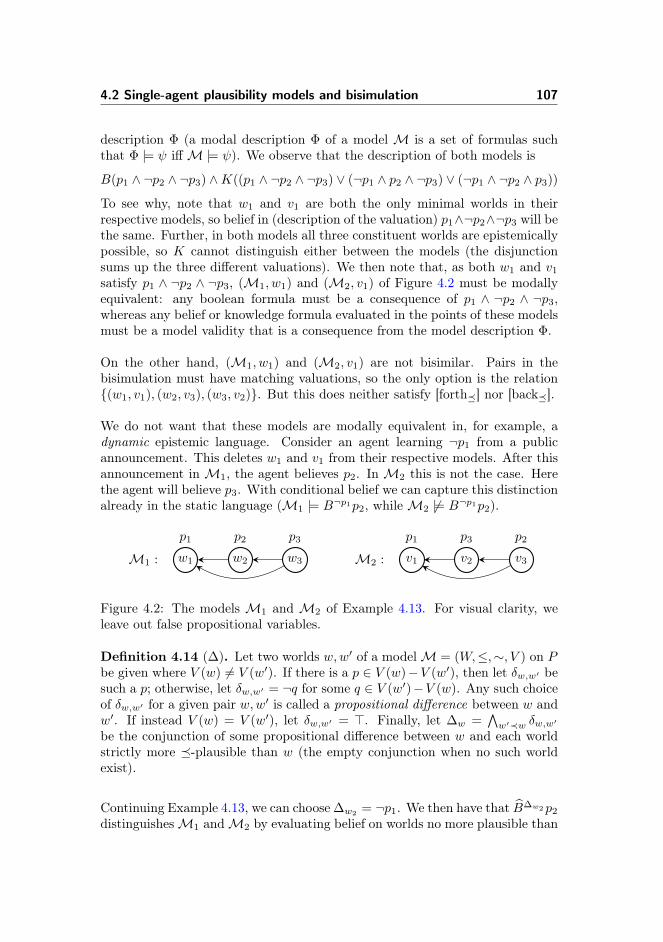
4.2 Single-agent plausibility models and bisimulation 107

description Φ (a modal description Φ of a model M is a set of formulas suchthat Φ |= ψ iffM |= ψ). We observe that the description of both models is

B(p1 ∧ ¬p2 ∧ ¬p3) ∧K((p1 ∧ ¬p2 ∧ ¬p3) ∨ (¬p1 ∧ p2 ∧ ¬p3) ∨ (¬p1 ∧ ¬p2 ∧ p3))

To see why, note that w1 and v1 are both the only minimal worlds in theirrespective models, so belief in (description of the valuation) p1∧¬p2∧¬p3 will bethe same. Further, in both models all three constituent worlds are epistemicallypossible, so K cannot distinguish either between the models (the disjunctionsums up the three different valuations). We then note that, as both w1 and v1

satisfy p1 ∧ ¬p2 ∧ ¬p3, (M1, w1) and (M2, v1) of Figure 4.2 must be modallyequivalent: any boolean formula must be a consequence of p1 ∧ ¬p2 ∧ ¬p3,whereas any belief or knowledge formula evaluated in the points of these modelsmust be a model validity that is a consequence from the model description Φ.

On the other hand, (M1, w1) and (M2, v1) are not bisimilar. Pairs in thebisimulation must have matching valuations, so the only option is the relation{(w1, v1), (w2, v3), (w3, v2)}. But this does neither satisfy [forth�] nor [back�].

We do not want that these models are modally equivalent in, for example, adynamic epistemic language. Consider an agent learning ¬p1 from a publicannouncement. This deletes w1 and v1 from their respective models. After thisannouncement inM1, the agent believes p2. InM2 this is not the case. Herethe agent will believe p3. With conditional belief we can capture this distinctionalready in the static language (M1 |= B¬p1p2, whileM2 6|= B¬p1p2).

w1

p1

w2

p2

w3

p3

M1 : v1

p1

v2

p3

v3

p2

M2 :

Figure 4.2: The models M1 and M2 of Example 4.13. For visual clarity, weleave out false propositional variables.

Definition 4.14 (∆). Let two worlds w,w′ of a modelM = (W,≤,∼, V ) on Pbe given where V (w) 6= V (w′). If there is a p ∈ V (w)−V (w′), then let δw,w′ besuch a p; otherwise, let δw,w′ = ¬q for some q ∈ V (w′)−V (w). Any such choiceof δw,w′ for a given pair w,w′ is called a propositional difference between w andw′. If instead V (w) = V (w′), let δw,w′ = >. Finally, let ∆w =

∧w′≺w δw,w′

be the conjunction of some propositional difference between w and each worldstrictly more �-plausible than w (the empty conjunction when no such worldexist).

Continuing Example 4.13, we can choose ∆w2 = ¬p1. We then have that B̂∆w2p2

distinguishesM1 andM2 by evaluating belief on worlds no more plausible than

108 Bisimulation for single-agent plausibility models

w2 and v2 respectively. However, choosing ∆w2 = p2 would not distinguish,so we add an additional disjunct for w3. Regardless of which propositionaldifferences are used in ∆w2

and ∆w3, B̂∆w2

∨∆w3p2 distinguishes the models.This is, of course, not sufficient for constructing distinguishing formulas in thegeneral case, but for our purposes of proving Proposition 4.16 it is enough.

Lemma 4.15. Let w and w′ be worlds of the model M = (W,≤,∼, V ) s.t.w′ � w, and ϕ a formula of LP , s.t. M, w′ |= ϕ. ThenM, w |= B̂∆w∨∆w′ϕ.

Proof. In the following we abbreviate ∆w∨∆w′ by ∆w,w′ . We need to show that∃u ∈ Min≤J∆w,w′KM, s.t. M, u |= ϕ. By construction of ∆w,w′ , we have thatfor all s ∈ J∆w,w′KM, either s ≈ w, s ≈ w′ or (w � s and w′ � s). By choiceof w and w′, we have w′ � w, meaning that ∃w′′ ∈ Min≤J∆w,w′KM such thatw′ ≈ w′′. Lemma 4.11 then says that w′ and w′′ are bisimilar, and Proposition4.12 that they are modally equivalent. ThusM, w′′ |= ϕ. This is the u we arelooking for, givingM, w |= B̂∆w,w′ϕ.

Proposition 4.16. On the class of image-finite models, modal equivalence im-plies bisimilarity.

Proof. Let M = (W,≤,∼, V ) and M′ = (W ′,≤′,∼′, V ′) be two image-finite,plausibility models on P , and define R ⊆ W ×W ′, such that (w,w′) ∈ R iff(M, w) ≡ (M′, w′). We show that R is in fact a bisimulation of the kind definedin Definition 4.9. Showing that R satisfies [atoms] is trivial. We skip the, lesstrivial, [forth∼], and [back∼] and show the considerably more complicated caseof [forth�] ([back�] is similar) as follows: Assume (M, w) ≡ (M′, w′), v ∈ Wand v � w and show that assuming that for all v′ ∈ W ′, v′ � w′ implies(M, v) 6≡ (M′, v′), leads to a contradiction. This then gives (M, v) ≡ (M′, v′)and therefore (v, v′) ∈ R.

Let S′ = {v′ | v′ � w′} = {v′1, . . . v′n} be the successors of w′. This set is finite,due to image-finiteness of the model. If v and no successor of w′ is modallyequivalent, there exists formulae ϕv

′i , such thatM, v |= ϕv

′i andM′, v′i 6|= ϕv

′i .

Therefore,M, v |= ϕv′1 ∧ · · · ∧ϕv′n . For notational ease, let Φ = ϕv

′1 ∧ · · · ∧ϕv′n .

WithM, v |= Φ, Lemma 4.15 givesM, w |= B̂∆w,vΦ (∆w,v is finite due to image-finiteness of the models). Now,M′, w′ |= B̂∆w,vΦ (which we must have due tomodal equivalence) iff there exists a u′ ∈ Min≤J∆w,vKM′ such thatM′, u′ |= Φ.By construction of Φ, no world v′i exists such that v′i � w′ andM′, v′i |= Φ, sowe must have w′ ≺ u′. There are two cases for (the weakest requirements for)

4.3 Degrees of belief and safe belief 109

this u′ to be minimal. Either (i) u′ ≤ w′ or (ii) w′ < u′ and w′ 6∈ J∆w,vKM′ .If (i) is the case, we must have a world w′′, with w′′ ≈ w′ and w′′ < u′, or wecouldn’t have w′ ≺ u′. But w′′ < u′ means that u′ cannot be minimal unlessw′ 6∈ J∆w,vKM′ , because otherwise w′′ ∈ J∆w,vKM′ . So, for (i) and (ii) both, wemust have w′ 6∈ J∆w,vKM′ . This yieldsM′, w′ |= ¬∆w,v. But asM, w |= ∆w,v,we get the sought after contradiction of (M, w) ≡ (M′, w′).

4.3 Degrees of belief and safe belief

In this section we sketch some further results that can be obtained for oursingle-agent setting of the logic of knowledge and conditional belief. Apartfrom conditional belief, other familiar epistemic notions in the philosophicallogical and artificial intelligence community are safe belief [Stalnaker, 1996] anddegrees of belief [Kraus et al., 1990, Spohn, 1988]. Our results generalize fairlystraightforwardly to such other notions. An agent has safe belief in formula ϕiff it will continue to believe ϕ no matter what true information conditions itsbelief.4

Definition 4.17 (Safe belief). We extend the inductive language definition witha clause 2ϕ for safe belief in ϕ. The semantics areM, w |= 2ϕ iff (M, w |= Bψϕfor all ψ such thatM, w |= ψ).

Degrees of belief are a quantitative alternative to conditional belief. The zerothdegree of belief B0ϕ is defeasible belief Bϕ as already defined. For M, w |=B1ϕ to hold ϕ should be true in (i) all minimal worlds accessible from w; butadditionally, (ii) if you take away those from the equivalence class, in all worldsthat are now minimal. If we do this with the normal plausibility relation weget what we want (otherwise, we run into the same problems as before — ourtreatment is not compatible with e.g. Spohn’s approach [Spohn, 1988], thatallows ‘gaps’ (layers without worlds) in between different degrees of belief).

Min0�[w]∼ := Min�([w]∼)

Minn+1� [w]∼ := Minn�[w]∼ if Minn�([w]∼) = [w]∼

Minn+1� [w]∼ := Minn�[w]∼ ∪Min�([w]∼ \Minn�[w]∼) otherwise

We now can define the logic of knowledge and degrees of belief.4This definition is conditional to modally definable subsets, unlike [Baltag and Smets,

2008, Stalnaker, 1996] where it is on any subset. In that case safe belief is not bisimulationinvariant and increases the expressivity of the logic.

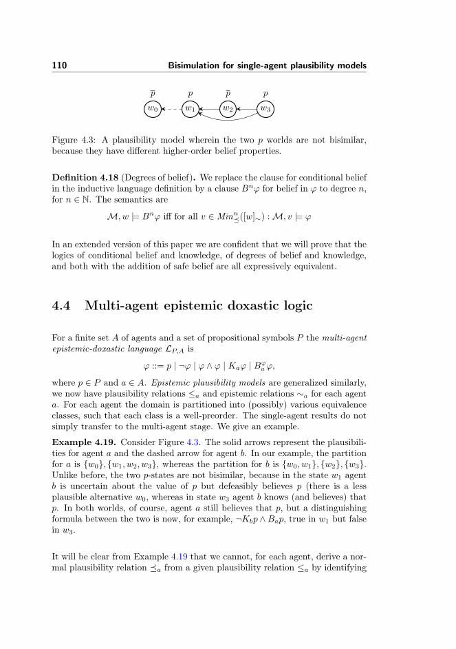
110 Bisimulation for single-agent plausibility models

w0

p

w1

p

w2

p

w3

p

Figure 4.3: A plausibility model wherein the two p worlds are not bisimilar,because they have different higher-order belief properties.

Definition 4.18 (Degrees of belief). We replace the clause for conditional beliefin the inductive language definition by a clause Bnϕ for belief in ϕ to degree n,for n ∈ N. The semantics are

M, w |= Bnϕ iff for all v ∈ Minn�([w]∼) :M, v |= ϕ

In an extended version of this paper we are confident that we will prove that thelogics of conditional belief and knowledge, of degrees of belief and knowledge,and both with the addition of safe belief are all expressively equivalent.

4.4 Multi-agent epistemic doxastic logic

For a finite set A of agents and a set of propositional symbols P the multi-agentepistemic-doxastic language LP,A is

ϕ ::= p | ¬ϕ | ϕ ∧ ϕ | Kaϕ | Bϕaϕ,

where p ∈ P and a ∈ A. Epistemic plausibility models are generalized similarly,we now have plausibility relations ≤a and epistemic relations ∼a for each agenta. For each agent the domain is partitioned into (possibly) various equivalenceclasses, such that each class is a well-preorder. The single-agent results do notsimply transfer to the multi-agent stage. We give an example.

Example 4.19. Consider Figure 4.3. The solid arrows represent the plausibili-ties for agent a and the dashed arrow for agent b. In our example, the partitionfor a is {w0}, {w1, w2, w3}, whereas the partition for b is {w0, w1}, {w2}, {w3}.Unlike before, the two p-states are not bisimilar, because in the state w1 agentb is uncertain about the value of p but defeasibly believes p (there is a lessplausible alternative w0, whereas in state w3 agent b knows (and believes) thatp. In both worlds, of course, agent a still believes that p, but a distinguishingformula between the two is now, for example, ¬Kbp ∧Bap, true in w1 but falsein w3.

It will be clear from Example 4.19 that we cannot, for each agent, derive a nor-mal plausibility relation �a from a given plausibility relation ≤a by identifying

4.5 Planning 111

worlds with the same valuation: w ≈a w′ iff V (w) = V (w′) and w ∼a w′ doesnot work (worlds w1 and w3 in Example 4.3 satisfy different formulas). Somestrengthening guarantees that bisimilarity still implies modal equivalence. Anexample is, using the above ≈a:

w ≈ w′ iff (for all agents a : w ≈a w′)w �a w′ iff (Min≤a [w]≈ ≤a Min≤a [w′]≈)

Unfortunately we do not get that modal equivalence then implies bisimilarity.The strongest possible approach is of course to require that [ w ≈ w′ iff (w,w′)is a pair in the bisimulation relation ]. This works, but it is is rather self-defeating. In due time we hope to find a proper generalisation in between thesetwo extremes.

4.5 Planning

In planning an agent is tasked with finding a course of action (i.e. a plan)that achieves a given goal. A planning problem implicitly represents a state-transition system, where transitions are induced by actions. Exploring thisstate-space is a common method for reasoning about and synthesising plans. Agrowing community investigates planning in dynamic epistemic logic [Bolanderand Andersen, 2011, Löwe et al., 2011, Aucher, 2012, Andersen et al., 2012], andusing the framework presented here we can in similar fashion consider planningwith doxastic attitudes. To this end we identify states with plausibility models,and the goal with a formula of the epistemic doxastic language. Further wecan describe the dynamics of actions by using e.g. hard announcements or softannouncements [van Benthem, 2007], or yet more expressive notions such asevent models [Baltag and Smets, 2008].

With the state-space consisting of plausibility models, model theoretic resultsbecome pivotal to the development of planning algorithms. In general, we cannotrequire even single-agent plausibility models (even on a finite set of propositionalsymbols) to be finite. Also, normal plausibility models need not be finite —obvious, as the ‘normalising’ procedure in which we replace ≤ by � does notchange the domain. Our definition of bisimulation has a crucial property in thisregard: By Lemma 4.11 the bisimulation contraction of a model will containno two worlds with the same valuation, hence any bisimulation minimal modelon a finite set of propositions is finite. Moreover, two bisimulation minimalmodels are bisimilar exactly when they are isomorphic, and it follows that areonly finitely many distinct bisimulation minimal epistemic plausibility models.With the reasonable assumption that actions preserve bisimilarity (this is thecase for the types of actions mentioned above), our investigations on the proper

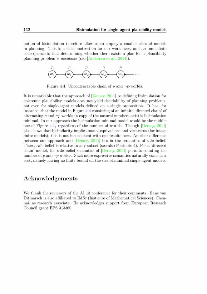
112 Bisimulation for single-agent plausibility models

notion of bisimulation therefore allow us to employ a smaller class of modelsin planning. This is a chief motivation for our work here, and an immediateconsequence is that determining whether there exists a plan for a plausibilityplanning problem is decidable (see [Andersen et al., 2014]).

w0

p

w1

p

w2

p

w3

p

w4

p

· · ·

Figure 4.4: Uncontractable chain of p and ¬p-worlds.

It is remarkable that the approach of [Demey, 2011] to defining bisimulation forepistemic plausibility models does not yield decidability of planning problems,not even for single-agent models defined on a single proposition. It has, forinstance, that the model in Figure 4.4 consisting of an infinite ‘directed chain’ ofalternating p and ¬p worlds (a copy of the natural numbers axis) is bisimulationminimal. In our approach the bisimulation minimal model would be the middleone of Figure 4.1, regardless of the number of worlds. Though [Demey, 2011]also shows that bisimilarity implies modal equivalence and vice versa (for imagefinite models), this is not inconsistent with our results here. Another differencebetween our approach and [Demey, 2011] lies in the semantics of safe belief.There, safe belief is relative to any subset (see also Footnote 4). For a ‘directedchain’ model, the safe belief semantics of [Demey, 2011] permits counting thenumber of p and ¬p worlds. Such more expressive semantics naturally come at acost, namely having no finite bound on the size of minimal single-agent models.

Acknowledgements

We thank the reviewers of the AI 13 conference for their comments. Hans vanDitmarsch is also affiliated to IMSc (Institute of Mathematical Sciences), Chen-nai, as research associate. He acknowledges support from European ResearchCouncil grant EPS 313360.

Chapter 5

Addendum to Bisimulationfor single-agent plausibilitymodels

Section 5.2 represents joint work between Mikkel Birkegaard Andersen,Thomas Bolander, Hans van Ditmarsch and this author. This work wasconducted during a research visit in Nancy, October 2013, and constitutespart of a joint journal publication not yet finalized. The presentation ofthe results in Section 5.2 is solely the work of this author. The other partsof this chapter are solely due to the author of this thesis.

In the previous chapter we presented a notion of bisimulation for single-agentplausibility models, and showed it to correspond with modal equivalence for thedoxastic language containing conditional belief. We further presented semanticsfor degrees of belief and safe belief, and briefly mentioned the role of modeltheory in planning — this chapter expands on exactly these topics. In Section5.1 we show that the notion of bisimulation in Definition 4.9 also correspondsto modal equivalence for the doxastic language containing degrees of belief.Following this, we use Section 5.2 to investigate the relative expressive power ofvarious doxastic languages, separated by which doxastic modalities are included.We conclude on our findings in Section 5.3, and additionally discuss furtherwork.

114 Addendum to Bisimulation for single-agent plausibility models

As we will consider different languages interpreted on plausibility models, westart things off by giving them distinct names. The language LP as it was namedin Chapter 4 is from this point on referred to as LCP , as it adds the conditionaldoxastic modality to the epistemic language. By LC,2P we denote the additionof the safe belief modality 2 to LCP , and in the usual way we define the dual 3ϕas ¬2¬ϕ. The semantics of safe belief is given below, where we also spell outthe semantics of its dual for convenience.

M, w |= 2ϕ iff (M, w |= Bψϕ for all ψ ∈ LCP such thatM, w |= ψ)

M, w |= 3ϕ iff (M, w |= B̂ψϕ for some ψ ∈ LCP such thatM, w |= ψ)

Turning to our quantitative doxastic modality, we let LDP denote the epistemiclanguage with the addition of Bn, referred to as either the degree of beliefmodality or quantitative doxastic modality. For some k ∈ N we let LD,kP ⊂ LDPdenote the language in which the maximum degree of the quantitative doxasticmodality is k.

5.1 Degrees of Belief

In this section we show how the quantitative doxastic modality matches upagainst the notion of bisimulation given in Definition 4.9. First we establish someresults regarding the relationship between Minn� and the normal plausibilityrelation. Next we apply these these results to show that the bisimulation foundDefinition 4.9 corresponds to modal equivalence for LDP (see Definition 3.3) inthe typical sense.

5.1.1 Belief Spheres and the Normal Plausibility Relation

For this subsection we letM = (W,≤,∼, V ) denote a plausibility model and �the normal plausibility relation of M. As ∼ is universal it is immediate that[w]∼ = W for any w ∈ W . Therefore Minn�[w]∼ is exactly Minn�W , so fornotational simplicity we use the latter form exclusively. We refer to the set ofworlds Minn�W as (belief) sphere n, and accordingly for w ∈ Minn�W we saythat w is in (belief) sphere n. The reading of Bnϕ is that ϕ is believed todegree n, where degrees should be determined in accordance with the normalplausibility relation �. As the semantics are given in terms of Minn�, we mustshow each belief sphere is in accord with �. By this we mean that there isno world w in sphere n, such that any world v not in sphere n is at least as

5.1 Degrees of Belief 115

plausible as w; i.e. v � w. Having shown this (see Proposition 5.2), we haveanother, equivalent, reading of Bnϕ, namely that ϕ is true in every world ofsphere n.

Lemma 5.1. Belief sphere n is a subset of belief sphere n+ 1.

Proof. Immediate from the recursive definition in Section 4.3.

Proposition 5.2. Any world in sphere n is strictly more plausible wrt. � thanany world not in sphere n.

Proof. Given worlds w, v ∈ W and any n ∈ N. We show that if w ∈ Minn�Wand v 6∈Minn�W , then w ≺ v. We proceed by induction on n. For the base caseassume that w ∈ Min0

�W and v 6∈ Min0�W . By �-minimality we have that

w � u for all u ∈W , and so also w � v. Assuming towards a contradiction thatv � w, we have from �-transitivity that v � u for all u ∈ W . But this leads tothe contradiction that v ∈ Min0

�W , and so we conclude v 6� w. We now havethat w ≺ v, settling the base case.

Assume now that w ∈ Minn+1W and v 6∈ Minn+1� W . By assumption sphere

n+1 must be a proper subset ofW , so we have that w ∈ (Minn�W ∪Min�(W \Minn�W )), which gives rise to two cases. If w ∈ Minn�W then it follows fromLemma 5.1 that v 6∈Minn�W , and so we have w ≺ v by applying the inductionhypothesis. Otherwise we have w ∈ Min�(W \ Minn�W ), and so from �-minimality it follows that w � u for all u ∈ (W \Minn�W ). With our initialassumption we have v ∈ (W \ (Minn�W ∪Min�(W \Minn�W ))), which impliesthat v ∈ (W \ Minn�W ) and consequently w � v. As in the base case theassumption of v � w leads to a contradiction, because we have v 6∈Min�(W \Minn�W ). As v 6� w we can conclude that w ≺ v.

Recall that the definition of minimality gives us that if w ∈Min�W then w � vfor any v ∈ W . However, this only holds for sphere 0; consider for instance aplausibility model with two worlds w, v where w ≺ v, we have v ∈Min1

�W butat the same time v 6� w. The issue here is that sphere 1 is a proper superset ofsphere 0. For worlds that just made the cut into a sphere, we have the followinguseful analogue.

Lemma 5.3. Given any n ∈ N and any w ∈ W . If w 6∈ Minn�W , then v � w

for any v ∈Minn+1� W .

Proof. We consider two exhaustive cases for v. Either v ∈ (Minn+1� W\Minn�W )

in which case v � w follows from minimality, since by assumption w ∈ (W \Minn�W ). Otherwise v ∈ Minn�W , and so from w 6∈ Minn�W and Proposition5.2 it follows that v ≺ w and hence also v � w.

116 Addendum to Bisimulation for single-agent plausibility models

Lemma 5.4. Worlds that are �-equiplausible belong to exactly the same beliefspheres.

Proof. We show that if v � w and w � v, then for any n ∈ N, w ∈ Minn�W iffv ∈ Minn�W . As � is a total preorder then by the assumption of v � w andw � v, it follows by minimality that for any subset W ′ ⊆ W : w ∈ Min�W

′

iff v ∈ Min�W′. Expanding the definitions of Minn�W and Minn�W we see

that both are unions of such �-minimal subsets of W , hence it follows thatw ∈Minn�W iff v ∈Minn�W .

Lemma 5.5. Worlds that have the same valuation belong to exactly the samebelief spheres.

Proof. Consider w, v ∈W where V (w) = V (v). Then w ≈ v and thusMin≤[w]≈ =Min≤[v]≈. By Definition 4.6 we have w � v and v � w, hence applying Lemma5.4 we arrive at the conclusion.

5.1.2 Bisimulation and Modal Equivalence for LDP

We now show that the notion of bisimulation is proper for plausibility modelswhen considering the language containing the quantitative doxastic modality.

Lemma 5.6. Let two plausibility models M = (W,≤,∼, V ), M′ = (W ′,≤′,∼′, V ′) with w ∈ W and w′ ∈ W ′ be given, and let �, �′ denote their respectivenormal plausibility relations. If R is a bisimulation between M and M′ where(w,w′) ∈ R, then for any n ∈ N, w ∈Minn�W iff w′ ∈Minn�′W

′.

Proof. Due to symmetry it is sufficient to show that w ∈ Minn�W impliesw′ ∈Minn�′W

′. We proceed by induction on n.

To show the base case let w ∈ Min0�W . Towards a contradiction assume that

w′ 6∈ Min0�W

′. Applying Proposition 5.2 this means there is a v′ ∈ Min0�′W

′

s.t. v′ �′ w′ and w′ 6�′ v′. From [back�] we have a v ∈ W s.t. v � w and(v, v′) ∈ R. As w is �-minimal in W we must have w � v. By [forth�] thereis u′ ∈ W ′ s.t. u′ �′ v′ and (w, u′) ∈ R, and since v′ is �′-minimal we haveu′ ∈ Min0

�W′. By [atoms] it follows that V (w) = V ′(w′) = V ′(u′), and so as

w′ ≈′ u′ we have by Lemma 5.5 that w′ ∈Min0�W

′, a contradiction.

For the induction step assume that w ∈Mink+1� W and let V = (W \Mink�W ).

With this definition of V we have that Mink+1� W = (Mink�W )∪ (Min�V ) and

further that (Mink�W ) ∩ V is the empty set. Therefore either w ∈ Mini�W

5.1 Degrees of Belief 117

for 0 ≤ i ≤ k, or w ∈ Min�V . In the former case we have w′ ∈ Mini�′W′

immediately from the induction hypothesis.

We can therefore assume for the remainder that w ∈ Min�V . Now let V ′ =(W ′ \ Mink�′W

′) and observe that Mink+1�′ W

′ = (Mink�′W′) ∪ (Min�′V

′).Towards a contradiction assume that w′ 6∈ Mink+1

�′ W′. By Proposition 5.2 we

therefore have a v′ ∈ Min�′V′ s.t. v′ � w′ and w′ 6� v′. This also implies

that v′ 6∈ Mink�′W′. By [back�] there is v ∈ W s.t. v � w and (v, v′) ∈ R. It

cannot be the case that v ∈ Mink�W , because the induction hypothesis wouldyield the contradiction v′ ∈ Mink�′W

′, and so we must have v ∈ V . As w is�-minimal in V it follows that w � v, and so by [forth�] there is u′ ∈ W ′ s.t.u′ � v′ and (w, u′) ∈ R. By [atoms] we have that V (w) = V ′(w′) = V ′(u′) andtherefore w′ ≈′ u′. By assumption of w′ 6∈ Mink+1

�′ W′ we can therefore apply

Lemma 5.5 to conclude that u′ 6∈ Mink+1�′ W

′. As v′ is in sphere k + 1, we canapply Proposition 5.2 to conclude v′ ≺ u′. But this contradicts u′ �′ v′, and soit must be the case that w′ ∈Mink+1

�′ W′.

Having shown that bisimilar worlds (even in different models) must have thesame degree of belief, the following is readily established.

Proposition 5.7. Bisimilarity implies modal equivalence for LDP .

Proof. We show that for all ϕ ∈ LDP , if (M, w) and (M′, w′) are bisimilar thenM, w |= ϕ iffM′, w′ |= ϕ. ForM = (W,≤,∼, V ) andM′ = (W,≤′,∼′, V ′), letR be a bisimulation s.t. (w,w′) ∈ R. We proceed by induction on the structureof ϕ, so by Proposition 4.12 we need only cover the case of Bnϕ.

We must show that M, w |= Bnϕ iff M′, w′ |= Bnϕ for any n ∈ N. Bysymmetry it suffices to show that M, w |= Bnϕ implies M′, w′ |= Bnϕ, whichmeans that M′, v′ |= ϕ for all v′ ∈ Minn�′W

′. So assume that M, w |= Bnϕ.For any v′ ∈Minn�′W

′ there will be (by totality of bisimulations) a v ∈ W s.t.(v, v′) ∈ R. By Lemma 5.6 it follows that v ∈Minn�W , and so by assumption ofM, w |= Bnϕ we haveM, v |= ϕ. By the induction hypothesis we can concludeM′, v′ |= ϕ, and so we haveM′, w′ |= Bnϕ.

As a brief intermission we remark that both ∼ and ≤ are primitives in ourplausibility models. So ifM is image-finite we require that for any world w ∈M,the sets {v ∈ W | v ∼ w} and {v ∈ W | v ≤ w} must be finite [Blackburnet al., 2001]. As ∼ is universal this has the very significant implication (whichis generally not the case for Kripke models) that any image-finite plausibilitymodels is in fact finite! Consequently we have that any belief sphere of animage-finite model is finite. We return to the business at hand, showing the

118 Addendum to Bisimulation for single-agent plausibility models

prototypical other direction of Proposition 5.7. To this end we first provide thecounterpart to Lemma 5.6 in the case of image-finite and modally equivalentmodels for LDP (for the notion of modal equivalence, see Definition 3.3).

Lemma 5.8. Let image-finite pointed plausibility models (M, w) and (M′, w′)whereM = (W,≤,∼, V ) andM′ = (W ′,≤′,∼′, V ′) be given. Further let �, �′denote their respective normal plausibility relations. If (M, w) ≡LD

P(M′, w′),

then for any n ∈ N it is the case that w ∈Minn�W iff w′ ∈Minn�′W′.

Proof. Due to symmetry we need only show left to right, so assume that w ∈Minn�W . Towards a contradiction assume that w′ 6∈ Minn�′W

′. For any v′ ∈Minn�′W

′ we therefore have that v′ is not in the same belief spheres as w′, so bythe contrapositive of Lemma 5.5 it follows that V ′(w′) 6= V ′(v′). Furthermore,as (M, w) ≡LD

P(M′, w′) it follows that V (w) = V ′(w′), and therefore also

V (w) 6= V ′(v′).

Having established this fact means we can find a simple formula γw,v′ for w andv′, which is true in w but false in v′. Formally, if there is a p ∈ (V (w) \ V ′(v′))then γw,v′ = p, and otherwise γw,v′ = ¬q for some q ∈ (V ′(v′) \ V (w)). Wedefine

Γnw =∧

v′∈Minn�′W

′

γw,v′

which is finite by image finiteness of M′. By construction we have that Γnwholds in w, but not in any world belonging to belief sphere n ofM′. In symbolsthis means thatM, w |= Γnw and by assumption of w ∈Minn�W it follows thatM, w |= B̂nΓnw. Furthermore, because there is no v′ ∈ Minn�′W

′ s.t. M′, v′ |=Γnw, we can conclude that M′, w′ 6|= B̂nΓnw. But this contradicts (M, w) ≡LD

P

(M′, w′) and consequently it must be the case that w′ ∈Minn�′W′

Having established this result, the following is shown using the same prooftechnique as in the Hennessy-Milner theorem.

Proposition 5.9. On the class of image-finite models, modal equivalence forLDP implies bisimilarity.

Proof. Let M = (W,≤,∼, V ) and M′ = (W ′,≤′,∼′, V ′) be two image-finite,plausibility models on P , and define R ⊆ W × W ′, such that (w,w′) ∈ Riff (M, w) ≡LD

P(M′, w′). We show that R satisfies the clauses in Definition

4.9, meaning that the ≡LDP

relation itself is a bisimulation. Foregoing [atoms],[forth∼] and [back∼], we will prove the most involved case [forth�] ([back�] canbe shown symmetrically).

5.2 Expressive power 119

Assume that (M, w) ≡LDP

(M′, w′), v ∈W and v � w. Towards a contradictionassume that there is no v′ ∈W ′ such that v′ �′ w′ and (M, v) ≡LD

P(M′, v′). Let

S′ = {v′ ∈ W ′ | v′ �′ w′} = {v′1, . . . v′m} be the �′-successors of w′ (S′ is finiteby image-finiteness ofM′). By assumption every v′i ∈ S′ is modally inequivalentto v, so for each v′i we have a formula ϕi s.t. M, v |= ϕi andM′, v′i 6|= ϕi. LettingΦ = ϕ1 ∧ · · · ∧ ϕm it follows thatM, v |= Φ andM′, v′i 6|= Φ.

If w ∈ Min0�W then v � w means that v ∈ Min0

�W , and so M, w |= B̂0Φ.Further, it follows from Lemma 5.8 that w′ ∈Min0

�′W′. By �-minimality of w′

in W ′ we have therefore that S′ = Min0�′W

′. By construction of Φ this meansthat M′, w′ 6|= B̂0Φ, contradicting the assumption that w and w′ are modallyequivalent.

If w 6∈ Min0�W , let n be chosen such that w ∈ Minn+1

� W and w 6∈ Minn�W .Such an n exists as W is finite. Since v � w, it must be the case that v ∈Minn+1

� W as Lemma 5.2 would otherwise imply w ≺ v. Therefore fromM, v |=Φ we have that M, w |= B̂n+1Φ. Moreover, by Lemma 5.8 it follows thatw′ ∈Minn+1

�′ W′ and w′ 6∈Minn�′W

′. By Lemma 5.3 we can therefore concludev′ �′ w′ for all v′ ∈ Minn+1

�′ W′ and hence Minn+1

�′ W′ ⊆ S′.1 By construction

of Φ this means there are no worlds inMinn+1�′ W

′ satisfying Φ, and soM′, w′ 6|=B̂nΦ. But this contradicts the assumption of (M, w) ≡LD

P(M′, w′).

Consequently we have that there must exist some v′ ∈ W ′ with v′ �′ w′ s.t.(M, v) ≡LD

P(M′, v′), showing that ≡LD

Psatisfies [forth�].

By going through the structural characterisation of bisimulation, we now havean immediate correspondence between modal equivalence for the language withconditional beliefs and modal equivalence for the language with degrees of belief.

Corollary 5.10. On the class of image-finite models, modal equivalence for LCPcorresponds to modal equivalence for LDP .

Proof. Left to right follows from Proposition 4.16 and Proposition 5.7. Right toleft follows similarly from 5.9 and Proposition 4.12.

5.2 Expressive power

This section represents joint work between Mikkel Birkegaard Andersen,1While sphere n is in fact exactly S′, this is not necessary to show for this proof.

120 Addendum to Bisimulation for single-agent plausibility models

Thomas Bolander, Hans van Ditmarsch and this author. This work wasconducted during a research visit in Nancy, October 2013, and constitutespart of a joint journal publication not yet finalized. The presentation ofthe results in this section is solely the work of this author.

Since we’re investigating different logical languages interpreted on the same classof models, there’s more to the story than bisimulation and modal equivalence.As we saw already in Example 4.13, having conditional belief allow us to distin-guish models which cannot be distinguished using only unconditional belief. Inthis sense conditional belief can express more properties of a model than uncon-ditional belief. Adopting this view of formulas we can for instance say that Bpqdescribes a certain property of plausibility models, namely that of plausibilitymodels in which, when given information that p is true, q is believed. Now wecan think of all the properties expressible using formulas of LCP as a benchmarkof how expressive the language with conditional belief really is. While gaugingexpressivity in absolute terms might provide further insight into a language,our main focus will be on the relative expressive power between LCP and thelanguages introduced above with different doxastic modalities.

In the next section we formally introduce the notion of expressive power, aswell as the notion of parameterized bisimulation. In Section 5.2.2 we showthat the language with conditional belief and the languages with degrees ofbelief are incomparable, and in Section 5.2.3 we show that adding safe belief tothe language with conditional belief yields a strictly more expressive language.This is in fact opposite of what we we’re confident could be proven at the end ofSection 4.3 (a carbon-copy of our original publication [Andersen et al., 2013]).

5.2.1 Formalities

We adopt the notions and basic concepts of the expressive power (or, expressiv-ity) of a language as presented in [van Ditmarsch et al., 2007]. We remind thereader that ϕ1 ≡ ϕ2 means that ϕ1 and ϕ2 are equivalent as per Definition 3.2.While ≡ is overloaded below, this introduces no ambiguity, as it will be clearfrom context whether we’re referring to models, formulas or languages.

Definition 5.11. Let L1 and L2 be languages interpreted in the same class ofmodels.

• L2 is at least as expressive as L1 (denoted L1 5 L2) iff for every ϕ1 ∈ L1

there is a ϕ2 ∈ L2 s.t. ϕ1 ≡ ϕ2.

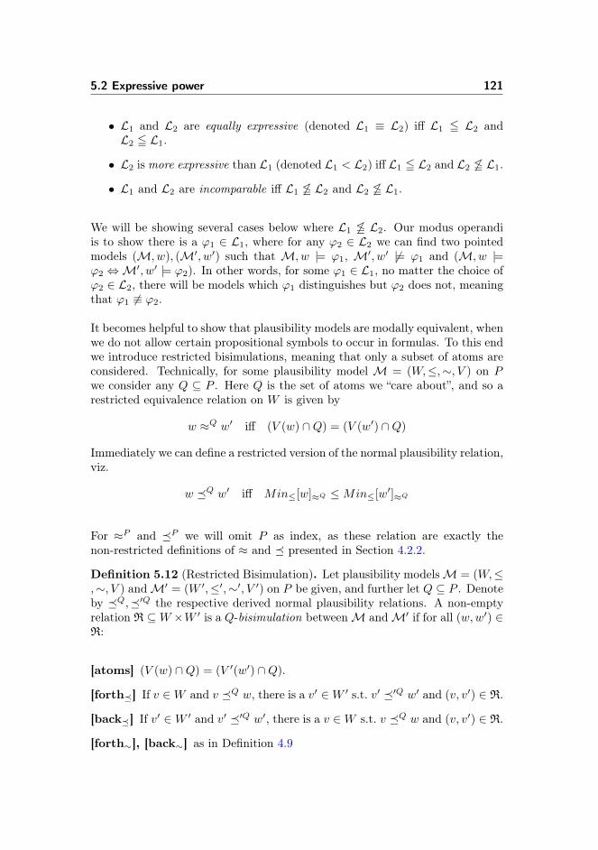
5.2 Expressive power 121

• L1 and L2 are equally expressive (denoted L1 ≡ L2) iff L1 5 L2 andL2 5 L1.

• L2 is more expressive than L1 (denoted L1 < L2) iff L1 5 L2 and L2 65 L1.

• L1 and L2 are incomparable iff L1 65 L2 and L2 65 L1.

We will be showing several cases below where L1 65 L2. Our modus operandiis to show there is a ϕ1 ∈ L1, where for any ϕ2 ∈ L2 we can find two pointedmodels (M, w), (M′, w′) such that M, w |= ϕ1, M′, w′ 6|= ϕ1 and (M, w |=ϕ2 ⇔M′, w′ |= ϕ2). In other words, for some ϕ1 ∈ L1, no matter the choice ofϕ2 ∈ L2, there will be models which ϕ1 distinguishes but ϕ2 does not, meaningthat ϕ1 6≡ ϕ2.

It becomes helpful to show that plausibility models are modally equivalent, whenwe do not allow certain propositional symbols to occur in formulas. To this endwe introduce restricted bisimulations, meaning that only a subset of atoms areconsidered. Technically, for some plausibility model M = (W,≤,∼, V ) on Pwe consider any Q ⊆ P . Here Q is the set of atoms we “care about”, and so arestricted equivalence relation on W is given by

w ≈Q w′ iff (V (w) ∩Q) = (V (w′) ∩Q)

Immediately we can define a restricted version of the normal plausibility relation,viz.

w �Q w′ iff Min≤[w]≈Q ≤Min≤[w′]≈Q

For ≈P and �P we will omit P as index, as these relation are exactly thenon-restricted definitions of ≈ and � presented in Section 4.2.2.

Definition 5.12 (Restricted Bisimulation). Let plausibility modelsM = (W,≤,∼, V ) andM′ = (W ′,≤′,∼′, V ′) on P be given, and further let Q ⊆ P . Denoteby �Q,�′Q the respective derived normal plausibility relations. A non-emptyrelation R ⊆W ×W ′ is a Q-bisimulation betweenM andM′ if for all (w,w′) ∈R:

[atoms] (V (w) ∩Q) = (V ′(w′) ∩Q).

[forth�] If v ∈W and v �Q w, there is a v′ ∈W ′ s.t. v′ �′Q w′ and (v, v′) ∈ R.

[back�] If v′ ∈W ′ and v′ �′Q w′, there is a v ∈W s.t. v �Q w and (v, v′) ∈ R.

[forth∼], [back∼] as in Definition 4.9

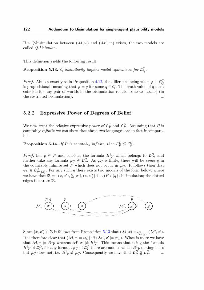
122 Addendum to Bisimulation for single-agent plausibility models

If a Q-bisimulation between (M, w) and (M′, w′) exists, the two models arecalled Q-bisimilar.

This definition yields the following result.

Proposition 5.13. Q-bisimilarity implies modal equivalence for LCQ.

Proof. Almost exactly as in Proposition 4.12, the difference being when ϕ ∈ LCQis propositional, meaning that ϕ = q for some q ∈ Q. The truth value of q mustcoincide for any pair of worlds in the bisimulation relation due to [atoms] (inthe restricted bisimulation).

5.2.2 Expressive Power of Degrees of Belief

We now treat the relative expressive power of LCP and LDP . Assuming that P iscountably infinite we can show that these two languages are in fact incompara-ble.

Proposition 5.14. If P is countably infinite, then LDP 65 LCP .

Proof. Let p ∈ P and consider the formula B1p which belongs to LDP , andfurther take any formula ϕC ∈ LCP . As ϕC is finite, there will be some q inthe countably infinite set P which does not occur in ϕC . It follows then thatϕC ∈ LCP\{q}. For any such q there exists two models of the form below, wherewe have that R = {(x, x′), (y, x′), (z, z′)} is a (P \ {q})-bisimulation; the dottededges illustrate R.

x

p, q

y

p

zM: x′

p

z′M′:

Since (x, x′) ∈ R it follows from Proposition 5.13 that (M, x) ≡LCP\{q}

(M′, x′).It is therefore clear that (M, x |= ϕC) iff (M′, x′ |= ϕC). What is more we havethat M, x |= B1p whereas M′, x′ 6|= B1p. This means that using the formulaB1p of LDP , for any formula ϕC of LCP there are models which B1p distinguishesbut ϕC does not; i.e. B1p 6≡ ϕC . Consequently we have that LDP 65 LCP .

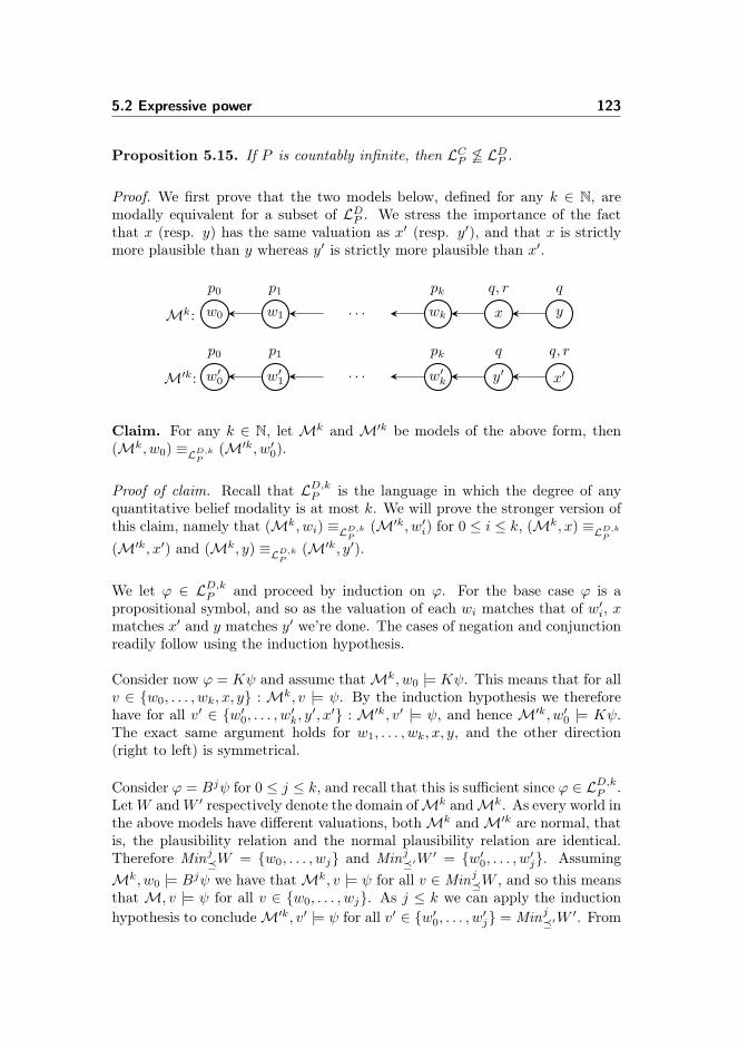
5.2 Expressive power 123

Proposition 5.15. If P is countably infinite, then LCP 65 LDP .

Proof. We first prove that the two models below, defined for any k ∈ N, aremodally equivalent for a subset of LDP . We stress the importance of the factthat x (resp. y) has the same valuation as x′ (resp. y′), and that x is strictlymore plausible than y whereas y′ is strictly more plausible than x′.

w0

p0

w1

p1

. . . wk

pk

x

q, r

y

q

Mk:

w′0

p0

w′1

p1

. . . w′k

pk

y′

q

x′

q, r

M′k:

Claim. For any k ∈ N, let Mk and M′k be models of the above form, then(Mk, w0) ≡LD,k

P(M′k, w′0).

Proof of claim. Recall that LD,kP is the language in which the degree of anyquantitative belief modality is at most k. We will prove the stronger version ofthis claim, namely that (Mk, wi) ≡LD,k

P(M′k, w′i) for 0 ≤ i ≤ k, (Mk, x) ≡LD,k

P

(M′k, x′) and (Mk, y) ≡LD,kP

(M′k, y′).

We let ϕ ∈ LD,kP and proceed by induction on ϕ. For the base case ϕ is apropositional symbol, and so as the valuation of each wi matches that of w′i, xmatches x′ and y matches y′ we’re done. The cases of negation and conjunctionreadily follow using the induction hypothesis.

Consider now ϕ = Kψ and assume thatMk, w0 |= Kψ. This means that for allv ∈ {w0, . . . , wk, x, y} : Mk, v |= ψ. By the induction hypothesis we thereforehave for all v′ ∈ {w′0, . . . , w′k, y′, x′} : M′k, v′ |= ψ, and hence M′k, w′0 |= Kψ.The exact same argument holds for w1, . . . , wk, x, y, and the other direction(right to left) is symmetrical.

Consider ϕ = Bjψ for 0 ≤ j ≤ k, and recall that this is sufficient since ϕ ∈ LD,kP .LetW andW ′ respectively denote the domain ofMk andMk. As every world inthe above models have different valuations, bothMk andM′k are normal, thatis, the plausibility relation and the normal plausibility relation are identical.Therefore Minj�W = {w0, . . . , wj} and Minj�′W

′ = {w′0, . . . , w′j}. AssumingMk, w0 |= Bjψ we have thatMk, v |= ψ for all v ∈ Minj�W , and so this meansthat M, v |= ψ for all v ∈ {w0, . . . , wj}. As j ≤ k we can apply the inductionhypothesis to concludeM′k, v′ |= ψ for all v′ ∈ {w′0, . . . , w′j} = Minj�′W

′. From

124 Addendum to Bisimulation for single-agent plausibility models

this it follows thatM′k, w′0 |= Bjψ as required. The same argument applies tow1, . . . , wk, x, y because Minj�W (i.e. belief sphere j) is unaltered by the worldin which Bjψ is evaluated (importantly, x and y are not in belief sphere k). Theother direction is shown symmetrically thus completing the proof of this claim.

Consider now Bqr belonging to LCP and any formula ϕD ∈ LDP . Since ϕD isfinite there is some k ∈ N such that ϕD ∈ LD,kP (e.g. take k to be the largestdegree of belief modality occurring in ϕD). By the above claim we thereforehave modelsMk andM′k such that (Mk, w0 |= ϕD)⇔ (M′k, w′0 |= ϕD). Thereason such models always exist is that p0, . . . , pk are taken from a countablyinfinite set of symbols and k ∈ N.

To determine the truth of Bqr we point out that [[q]]Mk = {x, y} and [[q]]M′k ={y′, x′}. Given the plausibility relation we have that conditional on q, x isminimal in Mk and y′ is minimal in M′k. Since Mk, x |= r and M′k, y′ 6|= r,it follows thatMk, w0 |= Bqr, whileM′k, w′0 6|= Bqr. With this we have shownthat taking the formula Bqr of LCP , there is for any ϕD ∈ LDP models which Bqrdistinguishes but ϕD does not; i.e. Bqr 6≡ ϕD. It follows that LCP 65 LDP .

The two propositions above yield the following result.

Corollary 5.16. If P is countably infinite, the languages LCP and LDP are in-comparable.

The proof of Proposition 5.14 illustrates the inability of conditional belief tocapture quantitative belief (even to degree 1), because the latter represents beliefthat is irrespective of some chosen facts. The proof of Proposition 5.15 showcasesthe ability of conditional belief to capture a form of quantitative belief to anarbitrary degree, with this degree depending on factual content (here simplyp) rather than a fixed number. In both proofs it is important that an infinitenumber of symbols are at our disposal. How the two languages compare whenP is finite has not been settled.

The incomparability of LCP and LDP is remarkable in light of Corollary 5.10, sincethe incomparability result is established without relying on image-infinite mod-els. Rather, we gave simple formulas in both languages that describe an infinitenumber of models, but which the other (respective) language cannot finitelycapture. Taking on a broader perspective this suggests that conditional beliefand degrees of belief should not be considered alternatives, but rather as com-plementary doxastic attitudes able to express different properties of plausibilitymodels.

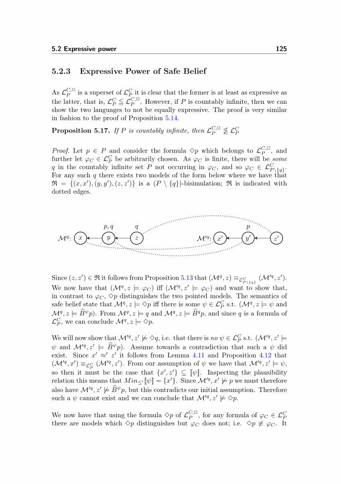
5.2 Expressive power 125

5.2.3 Expressive Power of Safe Belief

As LC,2P is a superset of LCP it is clear that the former is at least as expressive asthe latter, that is, LCP 5 L

C,2P . However, if P is countably infinite, then we can

show the two languages to not be equally expressive. The proof is very similarin fashion to the proof of Proposition 5.14.

Proposition 5.17. If P is countably infinite, then LC,2P 65 LCP

Proof. Let p ∈ P and consider the formula 3p which belongs to LC,2P , andfurther let ϕC ∈ LCP be arbitrarily chosen. As ϕC is finite, there will be someq in the countably infinite set P not occurring in ϕC , and so ϕC ∈ LCP\{q}.For any such q there exists two models of the form below where we have thatR = {(x, x′), (y, y′), (z, z′)} is a (P \ {q})-bisimulation; R is indicated withdotted edges.

x y

p, q

z

q

Mq: x′ y′

p

z′M′q:

Since (z, z′) ∈ R it follows from Proposition 5.13 that (Mq, z) ≡LCP\{q}

(M′q, z′).We now have that (Mq, z |= ϕC) iff (M′q, z′ |= ϕC) and want to show that,in contrast to ϕC , 3p distinguishes the two pointed models. The semantics ofsafe belief state thatMq, z |= 3p iff there is some ψ ∈ LCP s.t. (Mq, z |= ψ andMq, z |= B̂ψp). FromMq, z |= q andMq, z |= B̂qp, and since q is a formula ofLCP , we can concludeMq, z |= 3p.

We will now show thatM′q, z′ 6|= 3q, i.e. that there is no ψ ∈ LCP s.t. (M′q, z′ |=ψ and M′q, z′ |= B̂ψp). Assume towards a contradiction that such a ψ didexist. Since x′ ≈′ z′ it follows from Lemma 4.11 and Proposition 4.12 that(M′q, x′) ≡LC

P(M′q, z′). From our assumption of ψ we have thatM′q, z′ |= ψ,

so then it must be the case that {x′, z′} ⊆ [[ψ]]. Inspecting the plausibilityrelation this means thatMin≤′ [[ψ]] = {x′}. SinceM′q, x′ 6|= p we must thereforealso haveM′q, z′ 6|= B̂ψp, but this contradicts our initial assumption. Thereforesuch a ψ cannot exist and we can conclude thatM′q, z′ 6|= 3p.

We now have that using the formula 3p of LC,2P , for any formula of ϕC ∈ LCPthere are models which 3p distinguishes but ϕC does not; i.e. 3p 6≡ ϕC . It

126 Addendum to Bisimulation for single-agent plausibility models

therefore follows that LC,2P 65 LCP .

Corollary 5.18. If P is countably infinite, then LC,2P is more expressive thanLCP .

Safe belief enables us to express properties about infinitely many propositionswith a finite formula, exactly as was the case for degrees of a belief. This is whatprompts the increase in expressive power, again under the assumption that wehave infinitely many propositional symbols available, even though 2 is given itssemantics in terms of conditional belief.

Having established these results, we close with a few remarks about the lan-guages we have not treated. We use the obvious naming scheme for doing so.The languages L2

P and LD,2P cannot be dealt in our current setting, for 2 isgiven its semantics in terms of conditional belief. A trivial result is that LC,D,2P

is at least as expressive as both LC,DP and LC,2P as it subsumes both languages.Finally, assuming P is infinite it follows from Corollary 5.16 that LC,DP is moreexpressive than both LCP and LDP . Given the, at least to us, surprising natureof the results established in this section, we shall not dare to venture a guess asto how these other combinations relate, leaving these questions for future work.

5.3 Conclusion and Discussion

In this chapter we showed that the notion of bisimulation developed in Chap-ter 4 was also the right fit for capturing modal equivalence of LDP , that is, theextension of the epistemic language with a degrees of belief modality. Next, weproved several results on the expressive power of languages formed by differentcombinations of the conditional belief modality, the degrees of belief modalityand the safe belief modality. We showed that under the assumption of hav-ing an infinite number of propositional symbols given, the conditional beliefmodality and degree of belief modality are able to express different propertiesof plausibility models, and as such stand as genuine doxastic alternatives. Wefurthermore showed that the addition of the safe belief modality to LCP yields amore expressive language.

That our notion of bisimulation developed in Chapter 4 is also appropriatefor the language containing degrees of belief confirms our intuition that it isindeed the correct model-theoretic notion we have put forth. What is more, thisimplies that we can work with either or both modalities in a planning context,without increasing the size of contraction-minimal models nor the number of

5.3 Conclusion and Discussion 127

non-bisimilar information cells. That we may want to do so is apparent fromour expressivity results, for both modalities capture highly relevant aspects ofplanning with doxastic notions.

In terms of future work we have already accounted for the unresolved questionof how the languages compare for a finite number of propositions, and further-more noted languages that remains to be compared in terms of expressive power.Highly important to us is also the generalization of our notion of bisimulation tomulti-agent plausibility models, which is current work. Our preliminary resultsshow that there is a natural, albeit somewhat awkward, definition which cor-responds to modal equivalence for the multi-agent epistemic-doxastic languagecontaining the conditional belief modality. Such a result is vital for formalizingmulti-agent planning with doxastic attitudes.

128 Addendum to Bisimulation for single-agent plausibility models

Chapter 6

Don’t Plan for theUnexpected: Planning Basedon Plausibility Models

This chapter is a replicate of [Andersen et al., 2014], accepted for publicationin a special issue of Logique et Analyses devoted to the theme “Dynamics inLogic”.

130 Don’t Plan for the Unexpected: Planning Based on Plausibility Models

Don’t Plan for the Unexpected: Planning Basedon Plausibility Models

Mikkel Birkegaard Andersen Thomas BolanderMartin Holm Jensen

DTU Compute, Technical University of Denmark

Abstract

We present a framework for automated planning based on plau-sibility models, as well as algorithms for computing plans in thisframework. Our plausibility models include postconditions, as on-tic effects are essential for most planning purposes. The frameworkpresented extends a previously developed framework based on dy-namic epistemic logic (DEL), without plausibilities/beliefs. In thepure epistemic framework, one can distinguish between strong andweak epistemic plans for achieving some, possibly epistemic, goal.By taking all possible outcomes of actions into account, a strongplan guarantees that the agent achieves this goal. Conversely, aweak plan promises only the possibility of leading to the goal. Inreal-life planning scenarios where the planning agent is faced with ahigh degree of uncertainty and an almost endless number of possibleexogenous events, strong epistemic planning is not computationallyfeasible. Weak epistemic planning is not satisfactory either, as thereis no way to qualify which of two weak plans is more likely to lead tothe goal. This seriously limits the practical uses of weak planning,as the planning agent might for instance always choose a plan thatrelies on serendipity. In the present paper we introduce a planningframework with the potential of overcoming the problems of bothweak and strong epistemic planning. This framework is based on

132 Don’t Plan for the Unexpected: Planning Based on Plausibility Models

plausibility models, allowing us to define different types of plausibil-ity planning. The simplest type of plausibility plan is one in whichthe goal will be achieved when all actions in the plan turn out to havethe outcomes found most plausible by the agent. This covers manycases of everyday planning by human agents, where we—to limit ourcomputational efforts—only plan for the most plausible outcomes ofour actions.

6.1 Introduction

Whenever an agent deliberates about the future with the purpose of achievinga goal, she is engaging in the act of planning. Automated Planning is a widelystudied area of AI dealing with such issues under many different assumptionsand restrictions. In this paper we consider planning under uncertainty [Ghal-lab et al., 2004] (nondeterminism and partial observability), where the agenthas knowledge and beliefs about the environment and how her actions affectit. We formulate scenarios using plausibility models obtained by merging theframeworks in [Baltag and Smets, 2006, van Ditmarsch and Kooi, 2008].

Example 6.1 (The Basement). An agent is standing at the top of an unlitstairwell leading into her basement. If she walks down the steps in the dark, it’slikely that she will trip. On the other hand, if the lights are on, she is certain todescend unharmed. There is a light switch just next to her, though she doesn’tknow whether the bulb is broken.

She wishes to find a plan that gets her safely to the bottom of the stairs. Plan-ning in this scenario is contingent on the situation; e.g. is the bulb broken?Will she trip when attempting her descent? In planning terminology a planthat might achieve the goal is a weak solution, whereas one that guarantees itis a strong solution.

In this case, a weak solution is to simply descend the stairs in the dark, riskinglife and limb for a trip to the basement. On the other hand, there is no strongsolution as the bulb might be broken (assuming it cannot be replaced). Intu-itively, the best plan is to flick the switch (expecting the bulb to work) and thendescend unharmed, something neither weak nor strong planning captures.

Extending the approach in [Andersen et al., 2012] to a logical framework incor-porating beliefs via a plausibility ordering, we formalise plans which an agentconsiders most likely to achieve her goals. This notion is incorporated into al-gorithms developed for the framework in [Andersen et al., 2012], allowing us to

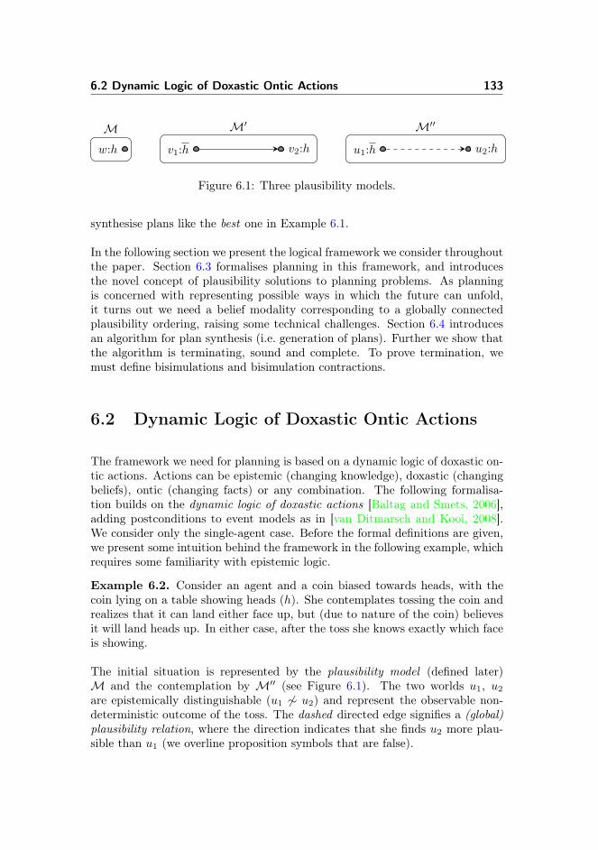
6.2 Dynamic Logic of Doxastic Ontic Actions 133

M M′ M′′

w:h v1:h v2:h u1:h u2:h

Figure 6.1: Three plausibility models.

synthesise plans like the best one in Example 6.1.

In the following section we present the logical framework we consider throughoutthe paper. Section 6.3 formalises planning in this framework, and introducesthe novel concept of plausibility solutions to planning problems. As planningis concerned with representing possible ways in which the future can unfold,it turns out we need a belief modality corresponding to a globally connectedplausibility ordering, raising some technical challenges. Section 6.4 introducesan algorithm for plan synthesis (i.e. generation of plans). Further we show thatthe algorithm is terminating, sound and complete. To prove termination, wemust define bisimulations and bisimulation contractions.

6.2 Dynamic Logic of Doxastic Ontic Actions

The framework we need for planning is based on a dynamic logic of doxastic on-tic actions. Actions can be epistemic (changing knowledge), doxastic (changingbeliefs), ontic (changing facts) or any combination. The following formalisa-tion builds on the dynamic logic of doxastic actions [Baltag and Smets, 2006],adding postconditions to event models as in [van Ditmarsch and Kooi, 2008].We consider only the single-agent case. Before the formal definitions are given,we present some intuition behind the framework in the following example, whichrequires some familiarity with epistemic logic.

Example 6.2. Consider an agent and a coin biased towards heads, with thecoin lying on a table showing heads (h). She contemplates tossing the coin andrealizes that it can land either face up, but (due to nature of the coin) believesit will land heads up. In either case, after the toss she knows exactly which faceis showing.

The initial situation is represented by the plausibility model (defined later)M and the contemplation by M′′ (see Figure 6.1). The two worlds u1, u2

are epistemically distinguishable (u1 6∼ u2) and represent the observable non-deterministic outcome of the toss. The dashed directed edge signifies a (global)plausibility relation, where the direction indicates that she finds u2 more plau-sible than u1 (we overline proposition symbols that are false).

134 Don’t Plan for the Unexpected: Planning Based on Plausibility Models

Example 6.3. Consider again the agent and biased coin. She now reasonsabout shuffling the coin under a dice cup, leaving the dice cup on top to concealthe coin. She cannot observe which face is up, but due to the bias of the coinbelieves it to be heads. She then reasons further about lifting the dice cup inthis situation, and realises that she will observe which face is showing. Due toher beliefs about the shuffle she finds it most plausible that heads is observed.

The initial situation is again M. Consider the model M′, where the soliddirected edge indicates a local plausibility relation, and the direction that v2 isbelieved over v1. By local we mean that the two worlds v1, v2 are (epistemically)indistinguishable (v1 ∼ v2), implying that she is ignorant about whether hor ¬h is the case.1 Together this represents the concealed, biased coin. Hercontemplations on lifting the cup is represented by the model M′′ as in theprevious example.

In Example 6.2 the agent reasons about a non-deterministic action whose out-comes are distinguishable but not equally plausible, which is different from theinitial contemplation in Example 6.3 where the outcomes are not distinguish-able (due to the dice cup). In Example 3 she subsequently reasons about theobservations made after a sensing action. In both examples she reasons aboutthe future, and in both cases the final result is the modelM′′. In Example 6.8we formally elaborate on the actions used here.

It is the nature of the agent’s ignorance that makeM′ andM′′ two inherentlydifferent situations. Whereas in the former she is ignorant about h due to thecoin being concealed, her ignorance in the latter stems from not having lifted thecup yet. In general we can model ignorance either as a consequence of epistemicindistinguishability, or as a result of not yet having acted. Neither type subsumesthe other and both are necessary for reasoning about actions. We capturethis distinction by defining both local and global plausibility relations. Theend result is that local plausibility talks about belief in a particular epistemicequivalence class, and global plausibility talks about belief in the entire model.We now remedy the informality we allowed ourselves so far by introducing thenecessary definitions for a more formal treatment.

Definition 6.4 (Dynamic Language). Let a countable set of propositional sym-bols P be given. The language L(P ) is given by the following BNF:

ϕ ::= p | ¬ϕ | ϕ ∧ ϕ | Kϕ | Bϕϕ | Xϕ | [E , e]ϕ

where p ∈ P , E is an event model on L(P ) as (simultaneously) defined below,1In the remainder, we use (in)distinguishability without qualification to refer to epistemic

(in)distinguishability.

6.2 Dynamic Logic of Doxastic Ontic Actions 135

and e ∈ D(E). K is the local knowledge modality, Bϕ the global conditionalbelief modality, X is a (non-standard) localisation modality (explained later)and [E , e] the dynamic modality.

We use the usual abbreviations for the other boolean connectives, as well asfor the dual dynamic modality 〈E , e〉ϕ := ¬ [E , e]¬ϕ and unconditional (orabsolute) global belief Bϕ := B>ϕ. The duals of K and Bϕ are denoted K̂ andB̂ϕ.

Kϕ reads as “the (planning) agent knows ϕ”, Bψϕ as “conditional on ψ, the(planning) agent believes ϕ”, and [E , e]ϕ as “after all possible executions of(E , e), ϕ holds”. Xϕ reads as “locally ϕ”.

Definition 6.5 (Plausibility Models). A plausibility model on a set of proposi-tions P is a tupleM = (W,∼,≤, V ), where

• W is a set of worlds,• ∼ ⊆W ×W is an equivalence relation called the epistemic relation,• ≤ ⊆W ×W is a connected well-preorder called the plausibility relation,2

• V : P → 2W is a valuation.

D(M) = W denotes the domain ofM. For w ∈ W we name (M, w) a pointedplausibility model, and refer to w as the actual world of (M, w). < denotes thestrict plausibility relation, that is w < w′ iff w ≤ w′ and w′ 6≤ w. ' denotesequiplausibility, that is w ' w′ iff w ≤ w′ and w′ ≤ w.

In our model illustrations a directed edge from w to w′ indicates w′ ≤ w. Byextension, strict plausibility is implied by unidirected edges and equiplausibilityby bidirected edges. For the models in Figure 6.1, we have v1 ∼ v2, v2 < v1 inM′ and u1 6∼ u2, u2 < u1 in M′′. The difference between these two models isin the epistemic relation, and is what gives rise to local (solid edges) and global(dashed edges) plausibility. In [Baltag and Smets, 2006] the local plausibilityrelation is defined as E:=∼ ∩ ≤; i.e. w E w′ iff w ∼ w′ and w ≤ w′. E is alocally well-preordered relation, meaning that it is a union of mutually disjointwell-preorders. Given a plausibility model, the domain of each element in thisunion corresponds to an ∼-equivalence class.

Our distinction between local and global is not unprecedented in the literature,but it can be a source of confusion. In [Baltag and Smets, 2006], ≤ was indeed

2A well-preorder is a reflexive, transitive binary relation s.t. every non-empty subset hasminimal elements [Baltag and Smets, 2008].

136 Don’t Plan for the Unexpected: Planning Based on Plausibility Models

connected (i.e. global), but in later versions of the framework [Baltag and Smets,2008] this was no longer required. The iterative development in [van Ditmarsch,2005] also discuss the distinction between local and global plausibility (namedpreference by the author). Relating the notions to the wording in [Baltag andSmets, 2006], ≤ captures a priori beliefs about virtual situations, before ob-taining any direct information about the actual situation. On the other hand,E captures a posteriori beliefs about an actual situation, that is, the agent’sbeliefs after she obtains (or assumes) information about the actual world.

M′′ represents two distinguishable situations (v1 and v2) that are a result ofreasoning about the future, with v2 being considered more plausible than v1.These situations are identified by restricting M′′ to its ∼-equivalence classes;i.e. M′′ � {v1} and M′′ � {v2}. Formally, given an epistemic model M,the information cells in M are the submodels of the form M � [w]∼ wherew ∈ D(M). We overload the term and name any ∼-connected plausibilitymodel on P an information cell. This use is slightly different from the notionin [Baltag and Smets, 2008], where an information cell is an ∼-equivalenceclass rather than a restricted model. An immediate property of informationcells is that ≤=E; i.e. the local and global plausibility relations are identical.A partition of a plausibility model into its information cells corresponds to alocalisation of the plausibility model, where each information cell represents alocal situation. The (later defined) semantics of X enables reasoning about suchlocalisations using formulas in the dynamic language.

Definition 6.6 (Event Models). An event model on the language L(P ) is atuple E = (E,∼,≤, pre, post), where

• E is a finite set of (basic) events,• ∼ ⊆ E × E is an equivalence relation called the epistemic relation,• ≤ ⊆ E × E is a connected well-preorder called the plausibility relation,• pre : E → L(P ) assigns to each event a precondition,• post : E → (P → L(P )) assigns to each event a postcondition for each

proposition. Each post(e) is required to be only finitely different from theidentity.

D(E) = E denotes the domain of E . For e ∈ E we name (E , e) a pointed eventmodel, and refer to e as the actual event of (E , e). We use the same conventionsfor accessibility relations as in the case of plausibility models.

Definition 6.7 (Product Update). Let M = (W,∼,≤, V ) and E = (E,∼′,≤′, pre, post) be a plausibility model on P resp. event model on L(P ). The productupdate ofM with E is the plausibility model denotedM⊗E = (W ′,∼′′,≤′′, V ′),where

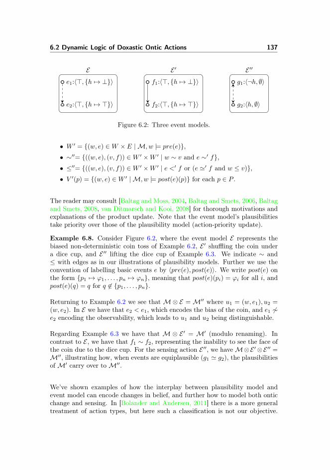
6.2 Dynamic Logic of Doxastic Ontic Actions 137

E E ′ E ′′

e1:〈>, {h 7→ ⊥}〉

e2:〈>, {h 7→ >}〉

f1:〈>, {h 7→ ⊥}〉

f2:〈>, {h 7→ >}〉

g1:〈¬h, ∅〉

g2:〈h, ∅〉

Figure 6.2: Three event models.

• W ′ = {(w, e) ∈W × E | M, w |= pre(e)},• ∼′′= {((w, e), (v, f)) ∈W ′ ×W ′ | w ∼ v and e ∼′ f},• ≤′′= {((w, e), (v, f)) ∈W ′ ×W ′ | e <′ f or (e '′ f and w ≤ v)},• V ′(p) = {(w, e) ∈W ′ | M, w |= post(e)(p)} for each p ∈ P .

The reader may consult [Baltag and Moss, 2004, Baltag and Smets, 2006, Baltagand Smets, 2008, van Ditmarsch and Kooi, 2008] for thorough motivations andexplanations of the product update. Note that the event model’s plausibilitiestake priority over those of the plausibility model (action-priority update).

Example 6.8. Consider Figure 6.2, where the event model E represents thebiased non-deterministic coin toss of Example 6.2, E ′ shuffling the coin undera dice cup, and E ′′ lifting the dice cup of Example 6.3. We indicate ∼ and≤ with edges as in our illustrations of plausibility models. Further we use theconvention of labelling basic events e by 〈pre(e), post(e)〉. We write post(e) onthe form {p1 7→ ϕ1, . . . , pn 7→ ϕn}, meaning that post(e)(pi) = ϕi for all i, andpost(e)(q) = q for q 6∈ {p1, . . . , pn}.

Returning to Example 6.2 we see thatM⊗ E = M′′ where u1 = (w, e1), u2 =(w, e2). In E we have that e2 < e1, which encodes the bias of the coin, and e1 6∼e2 encoding the observability, which leads to u1 and u2 being distinguishable.

Regarding Example 6.3 we have that M⊗ E ′ = M′ (modulo renaming). Incontrast to E , we have that f1 ∼ f2, representing the inability to see the face ofthe coin due to the dice cup. For the sensing action E ′′, we haveM⊗E ′⊗E ′′ =M′′, illustrating how, when events are equiplausible (g1 ' g2), the plausibilitiesofM′ carry over toM′′.

We’ve shown examples of how the interplay between plausibility model andevent model can encode changes in belief, and further how to model both onticchange and sensing. In [Bolander and Andersen, 2011] there is a more generaltreatment of action types, but here such a classification is not our objective.

138 Don’t Plan for the Unexpected: Planning Based on Plausibility Models

Instead we simply encode actions as required for our exposition and leave theseconsiderations as future work.

Among the possible worlds, ≤ gives an ordering defining what is believed. Givena plausibility model M = (W,∼,≤, V ), any non-empty subset of W will haveone or more minimal worlds with respect to ≤, since ≤ is a well-preorder. ForS ⊆W , the set of ≤-minimal worlds, denoted Min≤S, is defined as:

Min≤S = {s ∈ S | ∀s′ ∈ S : s ≤ s′}.

The worlds in Min≤S are called the most plausible worlds in S. The worldsof Min≤D(M) are referred to as the most plausible ofM. With belief definedvia minimal worlds (see the definition below), the agent has the same beliefs forany w ∈ D(M). Analogous to most plausible worlds, an information cellM′ ofM is called most plausible if D(M′) ∩Min≤D(M) 6= ∅ (M′ contains at leastone of the most plausible worlds ofM).

Definition 6.9 (Satisfaction Relation). Let a plausibility model M = (W,∼,≤, V ) on P be given. The satisfaction relation is given by, for all w ∈W :

M, w |= p iff w ∈ V (p)M, w |= ¬ϕ iff notM, w |= ϕM, w |= ϕ ∧ ψ iffM, w |= ϕ andM, w |= ψM, w |= Kϕ iffM, v |= ϕ for all w ∼ vM, w |= Bψϕ iffM, v |= ϕ for all v ∈Min≤{u ∈W | M, u |= ψ}M, w |= Xϕ iffM � [w]∼, w |= ϕM, w |= [E , e]ϕ iffM, w |= pre(e) impliesM⊗E , (w, e) |= ϕ

where ϕ,ψ ∈ L(P ) and (E , e) is a pointed event model. We write M |= ϕto mean M, w |= ϕ for all w ∈ D(M). Satisfaction of the dynamic modalityfor non-pointed event models E is introduced by abbreviation, viz. [E ]ϕ :=∧e∈D(E) [E , e]ϕ. Furthermore, 〈E〉ϕ := ¬ [E ]¬ϕ.3

The reader may notice that the semantic clause for M, w |= Xϕ is equivalentto the clause for M, w |= [E , e]ϕ when [E , e] is a public announcement of acharacteristic formula [van Benthem, 1998] being true exactly at the worlds in[w]∼ (and any other world modally equivalent to one of these). In this sense, theX operator can be thought of as a public announcement operator, but a specialone that always announces the current information cell. In the special casewhereM is an information cell, we have for all w ∈ D(M) thatM, w |= Xϕ iffM, w |= ϕ.

3Hence, M, w |= 〈E〉ϕ ⇔ M, w |= ¬ [E]¬ϕ ⇔ M, w |= ¬(∧

e∈D(E) [E, e]¬ϕ) ⇔ M, w |=∨e∈D(E) ¬ [E, e]¬ϕ⇔M, w |=

∨e∈D(E) 〈E, e〉ϕ.

6.3 Plausibility Planning 139

6.3 Plausibility Planning

The previous covered a framework for dealing with knowledge and belief in adynamic setting. In the following, we will detail how a rational agent wouldadapt these concepts to model her own reasoning about how her actions affectthe future. Specifically, we will show how an agent can predict whether or nota particular plan leads to a desired goal. This requires reasoning about theconceivable consequences of actions without actually performing them.

Two main concepts are required for our formulation of planning, both of whichbuild on notions from the logic introduced in the previous section. One isthat of states, a representation of the planning agent’s view of the world at aparticular time. Our states are plausibility models. The other concept is that ofactions. These represent the agent’s view of everything that can happen whenshe does something. Actions are event models, changing states into other statesvia product update.

In our case, the agent has knowledge and beliefs about the initial situation,knowledge and beliefs about actions, and therefore also knowledge and beliefsabout the result of actions.

All of what follows regards planning in the internal perspective. Section 6.3.1shows how plausibility models represent states, Section 6.3.2 how event mod-els represent actions and Section 6.3.3 how these ideas can formalise planningproblems with various kinds of solutions.

6.3.1 The Internal Perspective On States

In the internal perspective, an agent using plausibility models to represent herown view will, generally, not be able to point out the actual world. Consideragain the modelM in Figure 6.1, that has two indistinguishable worlds w1 andw2. IfM is the agent’s view of the situation, she will of course not be able tosay which is the actual world. If she was, then the model could not representthe situation where the two worlds are indistinguishable. By requiring the agentto reason from non-pointed plausibility models only (a similar argument makesthe case for non-pointed event models), we enforce the internal perspective.

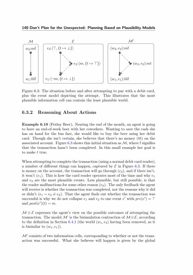
140 Don’t Plan for the Unexpected: Planning Based on Plausibility Models

M E M′

w1:mt

w2:mt

e1:〈¬m, {t 7→ ⊥}〉

e2:〈m, {t 7→ >}〉

e3:〈>, {t 7→ ⊥}〉

(w1, e1):mt

(w2, e3):mt

(w2, e2):mt

Figure 6.3: The situation before and after attempting to pay with a debit card,plus the event model depicting the attempt. This illustrates that the mostplausible information cell can contain the least plausible world.

6.3.2 Reasoning About Actions

Example 6.10 (Friday Beer). Nearing the end of the month, an agent is goingto have an end-of-week beer with her coworkers. Wanting to save the cash shehas on hand for the bus fare, she would like to buy the beer using her debitcard. Though she isn’t certain, she believes that there’s no money (m) on theassociated account. Figure 6.3 shows this initial situation asM, where t signifiesthat the transaction hasn’t been completed. In this small example her goal isto make t true.

When attempting to complete the transaction (using a normal debit card reader),a number of different things can happen, captured by E in Figure 6.3. If thereis money on the account, the transaction will go through (e2), and if there isn’t,it won’t (e1). This is how the card reader operates most of the time and why e1

and e2 are the most plausible events. Less plausible, but still possible, is thatthe reader malfunctions for some other reason (e3). The only feedback the agentwill receive is whether the transaction was completed, not the reasons why it didor didn’t (e1 ∼ e3 6∼ e2). That the agent finds out whether the transaction wassuccessful is why we do not collapse e1 and e2 to one event e′ with pre(e′) = >and post(e′)(t) = m.

M⊗ E expresses the agent’s view on the possible outcomes of attempting thetransaction. The modelM′ is the bisimulation contraction ofM⊗E , accordingto the definition in Section 6.4.1 (the world (w1, e3) having been removed, as itis bisimilar to (w1, e1)).

M′ consists of two information cells, corresponding to whether or not the trans-action was successful. What she believes will happen is given by the global

6.3 Plausibility Planning 141

plausibility relation. When actually attempting the transaction the result willbe one of the information cells of M′, namely Mt = M′ � {(w1, e1), (w2, e3)}or Mt = M′ � {(w2, e2)}, in which she will know ¬t and t respectively. As(w1, e1) is the most plausible, we can say that she expects to end up in (w1, e1),and, by extension, in the information cellMt: She expects to end up in a situ-ation where she knows ¬t, but is ignorant concerning m. If, unexpectedly, thetransaction is successful, she will know that the balance is sufficient (m). Themost plausible information cell(s) in a model are those the agent expects. That(w2, e3) is in the expected information cell, when the globally more plausibleworld (w2, e2) is not, might seem odd. It isn’t. The partitioning ofM into theinformation cells Mt and Mt suggests that she will sense the value of t (¬tholds everywhere in the former, t everywhere in the latter). As she expects tofind out that t does not to hold, she expects to be able to rule out all the worldsin which t does hold. Therefore, she expects to be able to rule out (w2, e2) andnot (w2, e3) (or w1, e1). This givesM′ |= BX(K¬t∧B¬m∧ K̂m): She expectsto come to know that the transaction has failed and that she will believe there’sno money on the account (though she does consider it possible that there is).

Under the definition of planning that is to follow in Section 6.3.3, an agent hasa number of actions available to construct plans. She needs a notion of whichactions can be considered at different stages of the planning process. As in theplanning literature, we call this notion applicability.

Definition 6.11 (Applicability). An event model E is said to be applicable ina plausibility modelM ifM |= 〈E〉>.

Unfolding the definition of 〈E〉, we see what applicability means:

M |= 〈E〉> ⇔ ∀w ∈ D(M) :M, w |= 〈E〉> ⇔∀w ∈ D(M) :M, w |= ∨e∈D(E) 〈E , e〉> ⇔∀w ∈ D(M),∃e ∈ D(E) :M, w |= 〈E , e〉> ⇔∀w ∈ D(M),∃e ∈ D(E) :M, w |= pre(e) andM⊗E , (w, e) |= > ⇔∀w ∈ D(M),∃e ∈ D(E) :M, w |= pre(e).

This says that no matter which is the actual world (it must be one of those con-sidered possible), the action defines an outcome. This concept of applicabilityis equivalent to the one in [Bolander and Andersen, 2011]. The discussion in[de Lima, 2007, sect. 6.6] also notes this aspect, insisting that actions must bemeaningful. The same sentiment is expressed by our notion of applicability.

Proposition 6.12. Given a plausibility modelM and an applicable event modelE, we have D(M⊗E) 6= ∅.

142 Don’t Plan for the Unexpected: Planning Based on Plausibility Models

M0

flick desc

w1:tlbsu w2:tlbsu

f1:〈t ∧ ¬s ∧ b, {l 7→ >, s 7→ >}〉

f2:〈t ∧ (s ∨ ¬b), {l 7→ ⊥, s 7→ ¬s}〉

e1:〈t, {t 7→ ⊥}〉

e2:〈t ∧ ¬l, {t 7→ ⊥, u 7→ ⊥}〉

Figure 6.4: An information cell,M0, and two event models, flick and desc.

The product updateM⊗E expresses the outcome(s) of doing E in the situationM, in the planning literature called applying E in M. The dynamic modality[E ] expresses reasoning about what holds after applying E .

Lemma 6.13. Let M be a plausibility model and E an event model. ThenM |= [E ]ϕ iffM⊗E |= ϕ.

Proof. M |= [E ]ϕ ⇔ ∀w ∈ D(M) :M, w |= [E ]ϕ ⇔∀w ∈ D(M) : M, w |=

∧e∈D(E)[E , e]ϕ ⇔ ∀(w, e) ∈ D(M) × D(E) : M, w |=

[E , e]ϕ ⇔∀(w, e) ∈ D(M)×D(E) :M, w |= pre(e) impliesM⊗E , (w, e) |= ϕ ⇔∀(w, e) ∈ D(M⊗E) :M⊗E , (w, e) |= ϕ ⇔ M⊗ E |= ϕ.

Here we are looking at global satisfaction, by evaluating [E ]ϕ in all ofM, ratherthan a specific world. The reason is that evaluation in planning must happenfrom the perspective of the planning agent and its “information state”. Thoughone of the worlds ofM is the actual world, the planning agent is ignorant aboutwhich it is. Whatever plan it comes up with, it must work in all of the worldswhich are indistinguishable to the agent, that is, in the entire model. A similarpoint, and a similar solution, is found in [Jamroga and Ågotnes, 2007].

Example 6.14. We now return to the agent from Example 6.1. Her view ofthe initial situation (M0) and her available actions (flick and desc) are seenin Figure 6.4. The propositional letters mean t: “top of stairs”, l: “light on”,b: “bulb working”, s : “switch on” and u: “unharmed”. Initially, in M0, shebelieves that the bulb is working, and knows that she is at the top of the stairs,unharmed and that the switch and light is off: M0 |= Bb ∧K(t ∧ u ∧ ¬l ∧ ¬s).

flick and desc represent flicking the light switch and trying to descend the stairs,respectively. Both require being at the top of the stairs (t). f1 of flick expressesthat if the bulb is working, turning on the switch will turn on the light, and f2

6.3 Plausibility Planning 143

M0 ⊗ flick

M0 ⊗ desc

(w1, f1):tlbsu (w2, f2):tlbsu

(w1, e1):tlbsu (w2, e1):tlbsu(w1, e2):tlbsu (w2, e2):tlbsu

Figure 6.5: The models resulting from applying the actions flick and desc inM0. Reflexive edges are not shown and the transitive closure is left implicit.

that if the bulb is broken or the switch is currently on, the light will be off. Theevents are epistemically distinguishable, as the agent will be able to tell whetherthe light is on or off. desc describes descending the stairs, with or without thelight on. e1 covers the agent descending the stairs unharmed, and can happenregardless of there being light or not. The more plausible event e2 representsthe agent stumbling, though this can only happen in the dark. If the light ison, she will descend safely. Definition 6.11 and Lemma 6.13 let us express theaction sequences possible in this scenario.

• M0 |= 〈flick〉> ∧ 〈desc〉>. The agent can initially do either flick or desc.

• M0 |= [flick] 〈desc〉>. After doing flick, she can do desc.

• M0 |= [desc] (¬ 〈flick〉> ∧ ¬ 〈desc〉>). Nothing can be done after desc.

Figure 6.5 shows the plausibility models arising from doing flick and desc inM0.Via Lemma 6.13 she can now conclude:

• M0 |= [flick] (Kb ∨ K¬b): Flicking the light switch gives knowledge ofwhether the bulb works or not.

• M0 |= [flick]BKb. She expects to come to know that it works.

• M0 |= [desc] (K¬t∧B¬u). Descending the stairs in the dark will definitelyget her to the bottom, though she believes she will end up hurting herself.

6.3.3 Planning

We now turn to formalising planning and then proceed to answer two questionsof particular interest: How do we verify that a given plan achieves a goal? Andcan we compute such plans? This section deals with the first question, planverification, while the second, plan synthesis, is detailed in Section 6.4.

144 Don’t Plan for the Unexpected: Planning Based on Plausibility Models

Definition 6.15 (Plan Language). Given a finite set A of event models onL(P ), the plan language L(P,A) is given by:

π ::= E | skip | if ϕ then π else π | π;π

where E ∈ A and ϕ ∈ L(P ). We name members π of this language plans, anduse if ϕ then π as shorthand for if ϕ then π else skip.

The reading of the plan constructs are “do E”, “do nothing”, “if ϕ then π, elseπ′”, and “first π then π′” respectively. In the translations provided in Definition6.16, the condition of the if-then-else construct becomes a K-formula, ensuringthat branching depends only on worlds which are distinguishable to the agent.The idea is similar to the meaningful plans of [de Lima, 2007], where branchingis allowed on epistemically interpretable formulas only.

Definition 6.16 (Translation). Let α be one of s, w, sp or wp. We define anα-translation as a function [·]α : L(P,A)→ (L(P )→ L(P )):

[E ]α ϕ := 〈E〉> ∧

[E ]XKϕ if α = s

K̂ 〈E〉XKϕ if α = w

[E ]BXKϕ if α = sp

[E ] B̂XKϕ if α = wp

[skip]α ϕ := ϕ

[if ϕ′ then π else π′]α ϕ := (Kϕ′ → [π]αϕ) ∧ (¬Kϕ′ → [π′]αϕ)

[π;π′]αϕ := [π]α([π′]αϕ)

We call [·]s the strong translation, [·]w the weak translation, [·]sp the strongplausibility translation and [·]wp the weak plausibility translation.

The translations are constructed specifically to make the following lemma hold,providing a semantic interpretation of plans (leaving out skip and π1;π2).

Lemma 6.17. LetM be an information cell, E an event model and ϕ a formulaof L(P ). Then:

1. M |= [E ]sϕ iff M |= 〈E〉> and for each information cell M′ of M⊗ E :M′ |= ϕ.

2. M |= [E ]wϕ iff M |= 〈E〉> and for some information cell M′ of M⊗ E :M′ |= ϕ.

6.3 Plausibility Planning 145

3. M |= [E ]spϕ iff M |= 〈E〉> and for each most plausible information cellM′ ofM⊗E :M′ |= ϕ.

4. M |= [E ]wpϕ iff M |= 〈E〉> and for some most plausible information cellM′ ofM⊗E :M′ |= ϕ.

5. M |= [if ϕ′ then π else π′]αϕ iff(M |= ϕ′ impliesM |= [π]αϕ) and (M 6|= ϕ′ impliesM |= [π′]αϕ).

Proof. We only prove 4 and 5, as 1–4 are very similar. For 4 we have:

M |= [E ]wp ϕ ⇔ M |= 〈E〉> ∧ [E ] B̂XKϕ ⇔Lemma 6.13

M |= 〈E〉> andM⊗E |= B̂XKϕ ⇔

M |= 〈E〉> and ∀(w, e) ∈ D(M⊗E) :M⊗E , (w, e) |= B̂XKϕ ⇔Prop. 6.12

M |= 〈E〉> and ∃(w, e) ∈Min≤D(M⊗E) :M⊗E , (w, e) |= XKϕ ⇔M |= 〈E〉> and ∃(w, e) ∈Min≤D(M⊗E) :M⊗E � [(w, e)]∼, (w, e) |= Kϕ ⇔M |= 〈E〉> and ∃(w, e) ∈Min≤D(M⊗E) :M⊗E � [(w, e)]∼ |= ϕ ⇔M |= 〈E〉> and in some most plausible information cellM′ ofM⊗E ,M′ |= ϕ.

For if-then-else, first note that:

M |= ¬Kϕ′ → [π]αϕ ⇔ ∀w ∈ D(M) :M, w |= ¬Kϕ′ → [π]αϕ ⇔∀w ∈ D(M) :M, w |= ¬Kϕ′ impliesM, w |= [π]αϕ ⇔M is an info. cell

∀w ∈ D(M) : ifM, v |= ¬ϕ′ for some v ∈ D(M) thenM, w |= [π]αϕ ⇔ifM, v |= ¬ϕ′ for some v ∈ D(M) then ∀w ∈ D(M) :M, w |= [π]αϕ ⇔M 6|= ϕ′ impliesM |= [π′]αϕ.

Similarly, we can prove:

M |= Kϕ′ → [π]αϕ ⇔ M |= Kϕ′ impliesM |= [π′]αϕ.

Using these facts, we get:

M |= [if ϕ′ then π else π′]αϕ ⇔ M |= (Kϕ′ → [π]αϕ) ∧ (¬Kϕ′ → [π′]αϕ) ⇔M |= Kϕ′ → [π]αϕ andM |= ¬Kϕ′ → [π′]αϕ ⇔(M |= ϕ′ impliesM |= [π]αϕ) and (M 6|= ϕ′ impliesM |= [π′]αϕ).

Using XK (as is done in all translations) means that reasoning after an action isrelative to a particular information cell (asM, w |= XKϕ⇔M � [w]∼, w |= Kϕ⇔ M � [w]∼ |= ϕ).

146 Don’t Plan for the Unexpected: Planning Based on Plausibility Models

Definition 6.18 (Planning Problems and Solutions). Let P be a finite set ofpropositional symbols. A planning problem on P is a triple P = (M0,A, ϕg)where

• M0 is a finite information cell on P called the initial state.

• A is a finite set of event models on L(P ) called the action library.

• ϕg ∈ L(P ) is the goal (formula).

A plan π ∈ L(P,A) is an α-solution to P if M0 |= [π]αϕg. For a specificchoice of α = s/w/sp/wp, we will call π a strong/weak/strong plausibility/weakplausibility-solution respectively.

Given a π, we wish to check whether π is an α-solution (for some particular α)to P. This can be done via model checking the dynamic formula given by thetranslation [π]α ϕg in the initial state of P.

A strong solution π is one that guarantees that ϕg will hold after executing it (“πachieves ϕg”). If π is a weak solution, it achieves ϕg for at least one particularsequence of outcomes. Strong and weak plausibility-solutions are as strong- andweak-solutions, except that they need only achieve ϕg for all of/some of themost plausible outcomes.

Example 6.19. The basement scenario (Example 6.1) can be formalised as theplanning problem PB = (M0, {flick, desc}, ϕg) with M0, flick and desc beingdefined in Figure 6.4 and ϕg = ¬t ∧ u. Let π1 = desc. We then have that:

M0 |= [desc]w (¬t ∧ u)⇔M0 |= 〈desc〉> ∧ K̂ 〈desc〉XK(¬t ∧ u)⇔desc is applic.

M0 |= K̂ 〈desc〉XK(¬t ∧ u)⇔ ∃w ∈ D(M0) :M0, w |= 〈desc〉XK(¬t ∧ u).

Picking w1, we have

M0, w1 |= 〈desc〉XK(¬t ∧ u)⇔M0 ⊗ desc, (w1, e1) |= XK(¬t ∧ u)⇔M0 ⊗ desc � [(w1, e1)]∼ |= (¬t ∧ u)

which holds as seen in Figure 6.5. Thus, π1 is a weak solution. Further, Lemma6.17 tells us that π1 is not a s/wp/sp solution, as u does not hold in the (mostplausible) information cellM⊗ desc � {(w1, e2), (w2, e2)}.

The plan π2 = flick; desc is a strong plausibility solution, as can be verified byM0 |= [π2]sp (¬t∧u). Without an action for replacing the lightbulb, there are nostrong solutions. Let replace be the action in Figure 6.6, where post(r1)(u) = ¬s

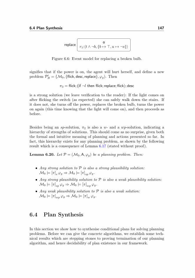
6.4 Plan Synthesis 147

replace r1:〈t ∧ ¬b, {b 7→ >, u 7→ ¬s}〉

Figure 6.6: Event model for replacing a broken bulb.

signifies that if the power is on, the agent will hurt herself, and define a newproblem P ′B = {M0, {flick, desc, replace}, ϕg). Then

π3 = flick; (if ¬l then flick; replace; flick); desc

is a strong solution (we leave verification to the reader): If the light comes onafter flicking the switch (as expected) she can safely walk down the stairs. Ifit does not, she turns off the power, replaces the broken bulb, turns the poweron again (this time knowing that the light will come on), and then proceeds asbefore.

Besides being an sp-solution, π2 is also a w- and a wp-solution, indicating ahierarchy of strengths of solutions. This should come as no surprise, given boththe formal and intuitive meaning of planning and actions presented so far. Infact, this hierarchy exists for any planning problem, as shown by the followingresult which is a consequence of Lemma 6.17 (stated without proof).

Lemma 6.20. Let P = (M0,A, ϕg) be a planning problem. Then:

• Any strong solution to P is also a strong plausibility solution:M0 |= [π]s ϕg ⇒M0 |= [π]sp ϕg.

• Any strong plausibility solution to P is also a weak plausibility solution:M0 |= [π]sp ϕg ⇒M0 |= [π]wp ϕg.

• Any weak plausibility solution to P is also a weak solution:M0 |= [π]wp ϕg ⇒M0 |= [π]w ϕg.

6.4 Plan Synthesis

In this section we show how to synthesise conditional plans for solving planningproblems. Before we can give the concrete algorithms, we establish some tech-nical results which are stepping stones to proving termination of our planningalgorithm, and hence decidability of plan existence in our framework.

148 Don’t Plan for the Unexpected: Planning Based on Plausibility Models

6.4.1 Bisimulations, contractions and modal equivalence

We now define bisimulations on plausibility models. For our purpose it is suf-ficient to define bisimulations on ∼-connected models, that is, on informationcells.4 First we define a normal plausibility relation which will form the basis ofour bisimulation definition.

Definition 6.21 (Normality). Given is an information cell M = (W,∼,≤, V )on P . By slight abuse of language, two worlds w,w′ ∈ W are said to have thesame valuation if for all p ∈ P : w ∈ V (p) ⇔ w′ ∈ V (p). Define an equivalencerelation on W : w ≈ w′ iff w and w′ has the same valuation. Now define w � w′iff Min≤([w]≈) ≤ Min≤([w′]≈). This defines the normal plausibility relation.M is called normal if � = ≤. The normalisation of M = (W,∼,≤, V ) isM′ = (W,∼,�, V ).

Definition 6.22 (Bisimulation). Let M = (W,∼,≤, V ) and M′ = (W ′,∼′,≤′, V ′) be information cells on P . A non-empty relation R ⊆ W ×W ′ is abisimulation between M and M′ (and M,M′ are called bisimilar) if for all(w,w′) ∈ R:

[atom] For all p ∈ P : w ∈ V (p) iff w′ ∈ V ′(p).

[forth] If v ∈W and v � w then there is a v′ ∈W ′ s.t. v′ �′ w′ and (v, v′) ∈ R.

[back] If v′ ∈W ′ and v′ � w′ then there is a v ∈W s.t. v � w and (v, v′) ∈ R.

If R has domain W and codomain W ′, it is called total. If M = M′, it iscalled an autobisimulation (onM). Two worlds w and w′ of an information cellM = (W,∼,≤, V ) are called bisimilar if there exists an autobisimulation R onM with (w,w′) ∈ R.

We are here only interested in total bisimulations, so, unless otherwise stated,we assume this in the following. Note that our definition of bisimulation imme-diately implies that there exists a (total) bisimulation between any informationcell and its normalisation. Note also that for normal models, the bisimulationdefinition becomes the standard modal logic one.5

4The proper notion of bisimulation for plausibility structures is explored in more detailby Andersen, Bolander, van Ditmarsch and Jensen in ongoing research. A similar notion forslightly different types of plausibility structures is given in [van Ditmarsch, pear]. Surprisingly,Demey does not consider our notion of bisimulation in his thorough survey [Demey, 2011] ondifferent notions of bisimulation for plausibility structures.

5We didn’t include a condition for the epistemic relation, ∼, in [back] and [forth], simplybecause we are here only concerned with ∼-connected models.

6.4 Plan Synthesis 149

Lemma 6.23. If two worlds of an information cell have the same valuationthey are bisimilar.

Proof. Assume worlds w and w′ of an information cellM = (W,∼,≤, V ) havethe same valuation. Let R be the relation that relates each world ofM to itselfand additionally relates w to w′. We want to show that R is a bisimulation.This amounts to showing [atom], [forth] and [back] for the pair (w,w′) ∈ R.[atom] holds trivially since w ≈ w′. For [forth], assume v ∈ W and v � w. Weneed to find a v′ ∈ W s.t. v′ � w′ and (v, v′) ∈ R. Letting v′ = v, it sufficesto prove v � w′. Since w ≈ w′ this is immediate: v � w ⇔ Min≤([v]≈) ≤Min≤([w]≈)

w≈w′⇔ Min≤([v]≈) ≤ Min≤([w′]≈) ⇔ v � w′. [back] is provedsimilarly.

Unions of autobisimulations are autobisimulations. We can then in the standardway define the (bisimulation) contraction of a normal information cell as itsquotient with respect to the union of all autobisimulations [Blackburn and vanBenthem, 2006].6 The contraction of a non-normal model is taken to be thecontraction of its normalisation. In a contracted model, no two worlds arebisimilar, by construction. Hence, by Lemma 6.23, no two worlds have thesame valuation. Thus, the contraction of an information cell on a finite set ofproposition symbols P contains at most 2|P | worlds. Since any information cellis bisimilar to its contraction [Blackburn and van Benthem, 2006], this showsthat there can only exist finitely many non-bisimilar information cells on anygiven finite set P .

Two information cells M and M′ are called modally equivalent, written M ≡M′, if for all formulas ϕ in L(P ): M |= ϕ ⇔ M′ |= ϕ. Otherwise, they arecalled modally inequivalent. We now have the following standard result (theresult is standard for standard modal languages and bisimulations, but it is nottrivial that it also holds here).

Theorem 6.24. If two information cells are (totally) bisimilar they are modallyequivalent.

Proof. We need to show that if R is a total bisimulation between informationcells M and M′, then for all formulas ϕ of L(P ): M |= ϕ ⇔ M′ |= ϕ. Firstwe show that we only have to consider formulas ϕ of the static sublanguage ofL(P ), that is, the language without the [E , e] modalities. In [Baltag and Smets,

6More precisely, let M be a normal information cell and let R be the union of all auto-bisimulations on M. Then the contraction M′ = (W ′,∼′,≤′, V ′) of M has as worlds theequivalence classes [w]R = {w′ | (w,w′) ∈ R} and has [w]R ≤′ [w′]R iff v ≤ v′ for somev ∈ [w]R and v′ ∈ [w′]R.

150 Don’t Plan for the Unexpected: Planning Based on Plausibility Models

2006], reduction axioms from the dynamic to the static language are given fora language similar to L(P ). The differences in language are our addition ofpostconditions and the fact that our belief modality is defined from the globalplausibility relation rather than being localised to epistemic equivalence classes.The latter difference is irrelevant when only considering information cells aswe do here. The former difference of course means that the reduction axiomspresented in [Baltag and Smets, 2006] will not suffice for our purpose. [vanDitmarsch and Kooi, 2008] shows that adding postconditions to the languagewithout the doxastic modalities only requires changing the reduction axiomfor [E , e] p, where p is a propositional symbol. Thus, if we take the reductionaxioms of [Baltag and Smets, 2006] and replace the reduction axiom for [E , e] pby the one in [van Ditmarsch and Kooi, 2008], we get reduction axioms for ourframework. We leave out the details.

We now need to show that if R is a total bisimulation between information cellsM andM′, then for all [E , e]-free formulas ϕ of L(P ): M |= ϕ⇔M′ |= ϕ. SinceR is total, it is sufficient to prove that for all [E , e]-free formulas ϕ of L(P ) and all(w,w′) ∈ R: M, w |= ϕ⇔M′, w′ |= ϕ. The proof is by induction on ϕ. In theinduction step we are going to need the induction hypothesis for several differentchoices of R, w and w′, so what we will actually prove by induction on ϕ is this:For all formulas ϕ of L(P ), if R is a total bisimulation between information cellsM andM′ on P and (w,w′) ∈ R, thenM, w |= ϕ⇔M′, w′ |= ϕ.

The base case is when ϕ is propositional. Then the required follows immediatelyfrom [atom], using that (w,w′) ∈ R. For the induction step, we have thefollowing cases of ϕ: ¬ψ,ψ ∧ γ,Xψ,Kψ,Bγψ. The first two cases are trivial.So is Xψ, as Xψ ↔ ψ holds on any information cell. For Kψ we reason asfollows. Let R be a total bisimulation between information cells M and M′with (w,w′) ∈ R. Using that R is total and that M and M′ are both ∼-connected we get: M, w |= Kψ ⇔ ∀v ∈ W : M, v |= ψ

i.h.⇔ ∀v′ ∈ W ′: M′, v |=ψ ⇔M′, w′ |= Kψ.

The case of Bγψ is more involved. Let M,M′,R, w and w′ be as above. Bysymmetry, it suffices to prove M, w |= Bγψ ⇒ M′, w′ |= Bγψ. So assumeM, w |= Bγψ, that is, M, v |= ψ for all v ∈ Min≤{u ∈ W | M, u |= γ}. Weneed to prove M′, v′ |= ψ for all v′ ∈ Min≤′{u′ ∈ W ′ | M′, u′ |= γ}. So letv′ ∈Min≤′{u′ ∈W ′ | M′, u′ |= γ}. By definition of Min≤′ this means that:

for all u′ ∈W ′, ifM′, u′ |= γ then v′ ≤′ u′. (6.1)

Choose an x ∈ Min≤{u ∈ W | u ≈ u′ and (u′, v′) ∈ R}. We want to use (6.1)to show that the following holds:

for all u ∈W , ifM, u |= γ then x ≤ u. (6.2)

6.4 Plan Synthesis 151

To prove (6.2), let u ∈ W withM, u |= γ. Choose u′ with (u, u′) ∈ R. The in-duction hypothesis impliesM′, u′ |= γ. We now prove that v′ ≤′ Min≤′([u

′]≈).To this end, let u′′ ∈ [u′]≈. We need to prove v′ ≤′ u′′. Since u′′ ≈ u′,Lemma 6.23 implies that u′ and u′′ are bisimilar. By induction hypothesis wethen getM′, u′′ |= γ.7 Using (6.1) we now get v′ ≤′ u′′, as required. This showv′ ≤′ Min≤′([u

′]≈). We now have Min≤′([v′]≈) ≤′ v′ ≤′ Min≤′([u

′]≈), andhence v′ � u′. By [back] there is then a v s.t. (v, v′) ∈ R and v � u. By choiceof x, x ≤ Min≤([v]≈). Using v � u, we now finally get: x ≤ Min≤([v]≈) ≤Min≤([u]≈) ≤ u. This shows that (6.2) holds.

From (6.2) we can now conclude x ∈ Min≤{u ∈ W | M, u |= γ} and hence,by original assumption, M, x |= ψ. By choice of x there is an x′ ≈ x with(x′, v′) ∈ R. Since M, x |= ψ and x′ ≈ x, we can again use Lemma 6.23 andthe induction hypothesis to conclude M, x′ |= ψ. Since (x′, v′) ∈ R, anotherinstance of the induction hypothesis gives usM′, v′ |= ψ, and we are done.

Previously we proved that there can only be finitely many non-bisimilar infor-mation cells on any finite set P . Since we have now shown that bisimilarityimplies modal equivalence, we immediately get the following result, which willbe essential to our proof of termination of our planning algorithms.

Corollary 6.25. Given any finite set P , there are only finitely many modallyinequivalent information cells on P .

6.4.2 Planning Trees

When synthesising plans, we explicitly construct the search space of the problemas a labelled and-or tree, a familiar model for planning under uncertainty[Ghallab et al., 2004]. Our and-or trees are called planning trees.

Definition 6.26 (Planning Tree). A planning tree is a finite, labelled and-ortree in which each node n is labelled by a plausibility model M(n), and eachedge (n,m) leaving an or-node is labelled by an event model E(n,m).

Planning trees for planning problems P = (M0,A, ϕg) are constructed as fol-lows: Let the initial planning tree T0 consist of just one or-node root(T0) withM(root(T0)) =M0 (the root labels the initial state). A planning tree for P isthen any tree that can be constructed from T0 by repeated applications of thefollowing non-deterministic tree expansion rule.

7Note that we here use the induction hypothesis for the autobisimulation on M′ linkingu′ and u′′, not the bisimulation R betweenM andM′.

152 Don’t Plan for the Unexpected: Planning Based on Plausibility Models

Definition 6.27 (Tree Expansion Rule). Let T be a planning tree for a planningproblem P = (M0,A, ϕg). The tree expansion rule is defined as follows. Pick anor-node n in T and an event model E ∈ A applicable inM(n) with the provisothat E does not label any existing outgoing edges from n. Then:

1. Add a new and-node m to T withM(m) =M(n)⊗ E , and add an edge(n,m) with E(n,m) = E .

2. For each information cellM′ inM(m), add an or-nodem′ withM(m′) =M′ and add the edge (m,m′).

The tree expansion rule is similar in structure to—and inspired by—the expan-sion rules used in tableau calculi, e.g. for modal and description logics [Horrockset al., 2006]. Note that the expansion rule applies only to or-nodes, and thatan applicable event model can only be used once at each node.

Considering single-agent planning a two-player game, a useful analogy for plan-ning trees are game trees. At an or-node n, the agent gets to pick any applicableaction E it pleases, winning if it ever reaches an information model in which thegoal formula holds (see the definition of solved nodes further below). At anand-node m, the environment responds by picking one of the information cellsof M(m)—which of the distinguishable outcomes is realised when performingthe action.

Without restrictions on the tree expansion rule, even very simple planning prob-lems might be infinitely expanded (e.g. by repeatedly choosing a no-op action).Finiteness of trees (and therefore termination) is ensured by the following block-ing condition.

B The tree expansion rule may not be applied to an or-node n for which thereexists an ancestor or-node m withM(m) ≡M(n).8

Lemma 6.28 (Termination). Any planning tree built by repeated application ofthe tree expansion rule under condition B is finite.

Proof. Planning trees built by repeated application of the tree expansion ruleare finitely branching: the action library is finite, and every plausibility modelhas only finitely many information cells (the initial state and all event models inthe action library are assumed to be finite, and taking the product update of a

8Modal equivalence between information cells can be decided by taking their respectivebisimulation contractions and then compare for isomorphism, cf. Section 6.4.1.

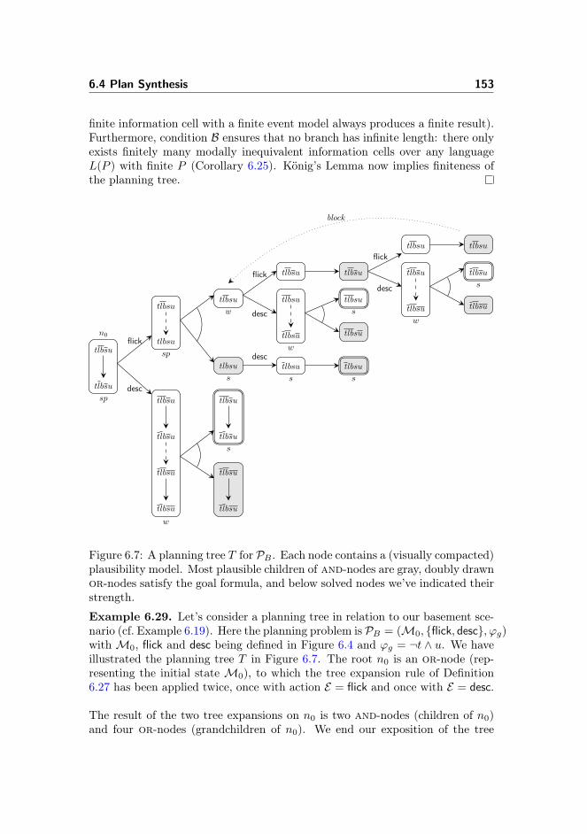
6.4 Plan Synthesis 153

finite information cell with a finite event model always produces a finite result).Furthermore, condition B ensures that no branch has infinite length: there onlyexists finitely many modally inequivalent information cells over any languageL(P ) with finite P (Corollary 6.25). König’s Lemma now implies finiteness ofthe planning tree.

n0

tlbsu

tlbsu

sp

tlbsu

tlbsu

sp

flick

tlbsu

s

tlbsu

w

tlbsuflick tlbsu

tlbsu

flicktlbsu

block

tlbsu

tlbsu

w

desc

tlbsu

tlbsu

s

tlbsu

tlbsu

w

desc

tlbsu

s

tlbsu

tlbsu

s

desctlbsu

s

tlbsu

tlbsu

tlbsu

tlbsu

w

desctlbsu

tlbsu

s

tlbsu

tlbsu

Figure 6.7: A planning tree T for PB . Each node contains a (visually compacted)plausibility model. Most plausible children of and-nodes are gray, doubly drawnor-nodes satisfy the goal formula, and below solved nodes we’ve indicated theirstrength.

Example 6.29. Let’s consider a planning tree in relation to our basement sce-nario (cf. Example 6.19). Here the planning problem is PB = (M0, {flick, desc}, ϕg)withM0, flick and desc being defined in Figure 6.4 and ϕg = ¬t ∧ u. We haveillustrated the planning tree T in Figure 6.7. The root n0 is an or-node (rep-resenting the initial state M0), to which the tree expansion rule of Definition6.27 has been applied twice, once with action E = flick and once with E = desc.

The result of the two tree expansions on n0 is two and-nodes (children of n0)and four or-nodes (grandchildren of n0). We end our exposition of the tree

154 Don’t Plan for the Unexpected: Planning Based on Plausibility Models

expansion rule here, and note that the tree has been fully expanded underthe blocking condition B, the dotted edge indicating a leaf having a modallyequivalent ancestor. Without the blocking condition, this branch could havebeen expanded ad infinitum.

Let T denote a planning tree containing an and-node n with a child m. Thenodem is called a most plausible child of n ifM(m) is among the most plausibleinformation cells ofM(n).

Definition 6.30 (Solved Nodes). Let T be any planning tree for a planningproblem P = (M0,A, ϕg). Let α be one of s, w, sp or wp. By recursivedefinition, a node n in T is called α-solved if one of the following holds:

• M(n) |= ϕg (the node satisfies the goal formula).• n is an or-node having at least one α-solved child.• n is an and-node and:

– If α = s then all children of n are α-solved.– If α = w then at least one child of n is α-solved.– If α = sp then all most plausible children of n are α-solved.– If α = wp then at least one of the most plausible children of n isα-solved.

Let T denote any planning tree for a planning problem P = (M0,A, ϕg). Belowwe show that when an or-node n of T is α-solved, it is possible to constructan α-solution to the planning problem (M(n),A, ϕg). In particular, if the rootnode is α-solved, an α-solution to P can be constructed. As it is never necessaryto expand an α-solved node, nor any of its descendants, we can augment theblocking condition B in the following way (parameterised by α where α is oneof s, w, sp or wp).

Bα The tree expansion rule may not be applied to an or-node n if one of thefollowing holds: 1) n is α-solved; 2) n has an α-solved ancestor; 3) n hasan ancestor or-node m withM(m) ≡M(n).

A planning tree that has been built according to Bα is called an α-planningtree. Since Bα is more strict than B, Lemma 6.28 immediately gives finiteness ofα-planning trees—and hence termination of any algorithm building such treesby repeated application of the tree expansion rule. Note that a consequence ofBα is that in any α-planning tree an α-solved or-node is either a leaf or hasexactly one α-solved child. We make use of this in the following definition.

6.4 Plan Synthesis 155

Definition 6.31 (Plans for Solved Nodes). Let T be any α-planning tree forP = (M0,A, ϕg). For each α-solved node n in T , a plan π(n) is defined recur-sively by:

• ifM(n) |= ϕg, then π(n) = skip.

• if n is an or-node and m its α-solved child, then π(n) = E(n,m);π(m).

• if n is an and-node and m1, . . . ,mk its α-solved children, then

– If k = 1 then π(n) = π(m1).– If k > 1 then for all i = 1, . . . , k let δmi

denote a formula true inM(mi) but not in any of theM(mj) 6≡ M(mi) and let π(n) =

if δm1 then π(m1) else if δm2 then π(m2) else · · · if δmkthen π(mk).

Note that the plan π(n) of a α-solved node n is only uniquely defined up to thechoice of δ-formulas in the if-then-else construct. This ambiguity in the definitionof π(n) will not cause any troubles in what follows, as it only depends on formulassatisfying the stated property. We need, however, to be sure that such formulasalways exist and can be computed. To prove this, assume n is an and-node andm1, . . . ,mk its α-solved children. Choose i ∈ {1, . . . , k}, and let mn1

, . . . ,mnl

denote the subsequence ofm1, . . . ,mk for whichM(mnj ) 6≡ M(mi). We need toprove the existence of a formula δmi such thatM(mi) |= δmi butM(mnj ) 6|= δmi

for all j = 1, . . . , l. Since M(mnj) 6≡ M(mi) for all j = 1, . . . , l, there exists

formulas δj such that M(mi) |= δj but M(mnj) 6|= δj . We then get that

δ1 ∧ δ2 ∧ · · · ∧ δl is true in M(mi) but none of the M(mnj). Such formulas

can definitely be computed, either by brute force search through all formulasordered by length or more efficiently and systematically by using characterisingformulas as in [Andersen et al., 2012] (however, characterising formulas for thepresent formalism are considerably more complex than in the purely epistemicframework of the cited paper).

Let n be a node of a planning tree T . We say that n is solved if it is α-solvedfor some α. If n is s-solved then it is also sp-solved, if sp-solved then wp-solved,and if wp-solved then w-solved. This gives a natural ordering s > sp > wp > w.Note the relation to Lemma 6.20. We say that a solved node n has strengthα, if it is α-solved but not β-solved for any β > α, using the aforementionedordering.

Example 6.32. Consider again the planning tree T in Figure 6.7 for the plan-ning problem PB = (M0, {flick, desc}, ϕg) with ϕg = ¬t ∧ u. Each solved nodehas been labelled by its strength. The reader is encouraged to check that eachnode has been labelled correctly according to Definition 6.30. The leafs satisfy-ing the goal formula ϕg have strength s, by definition. The strength of the root

156 Don’t Plan for the Unexpected: Planning Based on Plausibility Models

node is sp, as its uppermost child has strength sp. The reason this child hasstrength sp is that its most plausible child has strength s.

We see that T is an sp-planning tree, as it is possible to achieve T from n0

by applying tree expansions in an order that respects Bsp. However, it is notthe smallest sp-planning tree for the problem, as e.g. the lower subtree is notrequired for n0 to be sp-solved. Moreover, T is not a w-planning tree, as Bwwould have blocked further expansion once either of the three solved leafs wereexpanded.

In our soundness result below, we show that plans of α-solved roots are alwaysα-solutions to their corresponding planning problems. Applying Definition 6.31to the sp-planning tree T gives an sp-solution to the basement planning problem,viz. π(n0) = flick; desc; skip. This is the solution we referred to as the best inExample 6.1: Assuming all actions result in their most plausible outcomes, thebest plan is to flick the switch and then descend. After having executed thefirst action of the plan, flick, the agent will know whether the bulb is brokenor not. This is signified by the two distinct information cells resulting from theflick action, see Figure 6.7. An agent capable of replanning could thus chooseto revise her plan and/or goal if the bulb turns out to be broken.

Theorem 6.33 (Soundness). Let α be one of s, w, sp or wp. Let T be anα-planning tree for a problem P = (M0,A, ϕg) such that root(T ) is α-solved.Then π(root(T )) is an α-solution to P.

Proof. We need to prove that π(root(T )) is an α-solution to P, that is,M0 |=[π(root(T ))]α ϕg. Since M0 is the label of the root, this can be restated asM(root(T )) |= [π(root(T ))]α ϕg. To prove this fact, we will prove the followingstronger claim:

For each α-solved or-node n in T ,M(n) |= [π(n)]α ϕg.

We prove this by induction on the height of n. The base case is when n is aleaf (height 0). Since n is α-solved, we must have M(n) |= ϕg. In this caseπ(n) = skip. From M(n) |= ϕg we can conclude M(n) |= [skip]α ϕg, that is,M(n) |= [π(n)]α ϕg. This covers the base case. For the induction step, let n bean arbitrary α-solved or-node n of height h > 0. Let m denote the α-solvedchild of n, and m1, . . . ,ml denote the children of m. Let mn1 , . . . ,mnk

denotethe subsequence of m1, . . . ,ml consisting of the α-solved children of m. Then,by Definition 6.31,

• If k = 1 then π(n) = E(n,m);π(mn1).

• If k > 1 then π(n) = E(n,m);π(m) where π(m) =if δmn1

then π(mn1) else if δmn2

then π(mn2) else · · · if δmnk

then π(mnk).

6.4 Plan Synthesis 157

We here consider only the (more complex) case k > 1. Our goal is to proveM(n) |= [π(n)]α ϕg, that is, M(n) |= [E(n,m);π(m)]α ϕg. By the inductionhypothesis we haveM(mni

) |= [π(mni)]α ϕg for all i = 1, . . . , k (the mni

are oflower height than n).

Claim 1. M(mni) |= [π(m)]α ϕg for all i = 1, . . . , k.

Proof of claim. Let i be given. We need to prove

M(mni) |=

[if δmn1

then π(mn1) else · · · if δmnk

then π(mnk)]αϕg.

Note that by using item 5 of Lemma 6.17 it suffices to prove that for all j =1, . . . , k,

M(mni) |= δmnj

impliesM(mni) |=

[π(mnj

)]αϕg. (6.3)

Let j ∈ {1, . . . , k} be chosen arbitrarily. Assume first j = i. By induc-tion hypothesis we have M(mnj ) |=

[π(mnj )

]αϕg, and hence M(mni) |=[

π(mnj)]αϕg. From this (6.3) immediately follows. Assume now j 6= i. By the

construction of the δ-formulas, eitherM(mnj ) ≡M(mni) orM(mni) 6|= δmnj.

In the latter case, (6.3) holds trivially. In case of M(mnj) ≡ M(mni

) we im-mediately getM(mni

) |=[π(mnj

)]αϕg, since by induction hypothesis we have

M(mnj) |=

[π(mnj

)]αϕg. This concludes the proof of the claim.

Note that by definition of the tree expansion rule (Definition 6.27),M(m1), . . . ,M(ml)are the information cells inM(m).

Claim 2. The following holds:

• If α = s (w), then for every (some) information cellM′ inM(m): M′ |=[π(m)]α ϕg.

• If α = sp (wp), then for every (some) most plausible information cellM′inM(m): M′ |= [π(m)]α ϕg.

Proof of claim. We only consider the most complex cases, α = sp and α = wp.First consider α = sp. Let M′ be a most plausible information cell in M(m).We need to proveM′ |= [π(m)]α ϕg. Since, as noted above,M(m1), . . . ,M(ml)are the information cells in M(m), we must have M′ = M(mi) for some i ∈{1, . . . , l}. Furthermore, asM′ is among the most plausible information cells inM(m), mi must by definition be a most plausible child of m. Definition 6.30then gives us that mi is α-solved. Thus mi = mnj for some j ∈ {1, . . . , k}. ByClaim 1 we have M(mnj ) |= [π(m)]α ϕg, and since M′ = M(mi) = M(mnj )this gives the desired conclusion. Now consider the case α = wp. Definition 6.30

158 Don’t Plan for the Unexpected: Planning Based on Plausibility Models

gives us that at least one of the most plausible children of m are α-solved.By definition, this must be one of the mni

, i ∈ {1, . . . , k}. Claim 1 givesM(mni

) |= [π(m)]α ϕg. Since mniis a most plausible child of m, we must have

that M(mni) is among the most plausible information cells in M(m). Hence

we have proven that [π(m)]α ϕg holds in a most plausible information cell ofM(m).

By definition of the tree expansion rule (Definition 6.27), M(m) = M(n) ⊗E(n,m). Thus we can replaceM(m) byM(n)⊗E(n,m) in Claim 2 above. Usingitems 1–4 of Lemma 6.17, we immediately get from Claim 2 that independentlyof α the following holds: M(n) |= [E(n,m)]α [π(m)]α ϕg (the conditionM(n) |=〈E(n,m)〉> holds trivially by the tree expansion rule). From this we can thenfinally concludeM(n) |= [E(n,m);π(m)]α ϕg, as required.

Theorem 6.34 (Completeness). Let α be one of s, w, sp or wp. If there is anα-solution to the planning problem P = (M0,A, ϕg), then an α-planning tree Tfor P can be constructed, such that root(T ) is α-solved.

Proof. First note that we have [skip;π]α ϕg = [skip]α ([π]α ϕg) = [π]α ϕg. Thus,we can without loss of generality assume that no plan contains a subexpressionof the form skip;π. The length of a plan π, denoted |π|, is defined recursivelyby: |skip| = 1; |E| = 1; |if ϕ then π1 else π2| = |π1|+ |π2|; |π1;π2| = |π1|+ |π2|.

Claim 1. Let π be an α-solution to P = (M0,A, ϕg) with |π| ≥ 2. Then thereexists an α-solution of the form E ;π′ with |E ;π′| ≤ |π|.

Proof of claim. Proof by induction on |π|. The base case is |π| = 2. We have twocases, π = if ϕ then π1 else π2 and π = π1;π2, both with |π1| = |π2| = 1. If π isthe latter, it already has desired the form. If π = if ϕ then π1 else π2 then, byassumption on π, M0 |= [if ϕ then π1 else π2]α ϕg. Item 5 of Lemma 6.17 nowgives thatM0 |= ϕ impliesM0 |= [π1]α ϕg andM0 6|= ϕ impliesM0 |= [π2]α ϕg.Thus we must either haveM0 |= [π1]α ϕg orM0 |= [π2]α ϕg, that is, either π1

or π2 is an α-solution to P. Thus either π1; skip or π2; skip is an α-solution toP, and both of these have length |π|. This completes the base case. For theinduction step, consider a plan π of length l > 2 which is an α-solution to P.We again have two cases to consider, π = if ϕ then π1 else π2 and π = π1;π2.If π = π1;π2 is an α-solution to P, then π1 is an α-solution to the planningproblem P ′ = (M0,A, [π2]α ϕg), asM0 |= [π1;π2]α ϕg ⇔M0 |= [π1]α [π2]α ϕg.Clearly |π1| < l, so the induction hypothesis gives that there is an α-solution(E ;π′1) to P ′, with |E ;π′1| ≤ |π1|. Then, E ;π′1;π2 is an α-solution to P and wehave |E ;π′1;π2| = |E ;π′1|+ |π2| ≤ |π1|+ |π2| = |π|. If π = if ϕ then π1 else π2 isan α-solution to P, then we can as above conclude that either π1 or π2 is anα-solution to P. With both |π1| < l and |π2| < l, the induction hypothesis gives

6.4 Plan Synthesis 159

the existence an α-solution E ;π′, with |E ;π′| ≤ |π|. This completes the proof ofthe claim.

We now prove the theorem by induction on |π|, where π is an α-solution toP = (M0,A, ϕg). We need to prove that there exists an α-planning tree forP in which the root is α-solved. Let T0 denote the planning tree for P onlyconsisting of its root node with labelM0. The base case is when |π| = 1. Here,we have two cases, π = skip and π = E . In the first case, the planning treeT0 already has its root α-solved, since M0 |= [skip]α ϕg ⇔ M0 |= ϕg. In thesecond case, π = E , we haveM0 |= [E ]α ϕg as π = E is an α-solution to P. Bydefinition, this means that E is applicable in M0, and we can apply the treeexpansion rule to T0, which will produce:

1. A child m of the root node withM(m) =M0 ⊗ E .2. Children m1, . . . ,ml of m, whereM(m1), . . . ,M(ml) are the information

cells ofM(m).

Call the expanded tree T1. Since M0 |= [E ]α ϕg, Lemma 6.17 implies that forevery/some/every most plausible/some most plausible information cell M′ inM0 ⊗ E , M′ |= ϕg (where α = s/w/sp/wp). Since M(m1), . . . ,M(ml) arethe information cells ofM0 ⊗ E , we can conclude that every/some/every mostplausible/some most plausible child of m is α-solved. Hence also m and thus nare α-solved. The base is hereby completed.

For the induction step, let π be an α-solution to P with length l > 1. Let T0

denote the planning tree for P consisting only of its root node with labelM0. ByClaim 1, there exists an α-solution to P of the form E ;π′ with |E ;π′| ≤ |π|. AsM0 |= [E ;π′]α ϕg ⇔M0 |= [E ]α [π′]α ϕg, E is applicable inM0. Thus, as in thebase case, we can apply the tree expansion rule to T0 which will produce nodesas in 1 and 2 above. Call the expanded tree T1. SinceM0 |= [E ]α [π′]α ϕg, items1–4 of Lemma 6.17 implies that for every/some/every most plausible/some mostplausible information cell inM0⊗E , [π′]α ϕg holds. Hence, for every/some/everymost plausible/some most plausible child mi of m, M(mi) |= [π′]α ϕg. Letmn1

, . . . ,mnkdenote the subsequence of m1, . . . ,ml consisting of the children

of m for which M(mni) |= [π′]α ϕg. Then, by definition, π′ is an α-solutionto each of the planning problem Pi = (M(mni),A, ϕg), i = 1, . . . , k. As |π′| <|E ;π′| ≤ l, the induction hypothesis gives that α-planning trees T ′i with α-solvedroots can be constructed for each Pi. Let T2 denote T1 expanded by adding eachplanning tree T ′i as the subtree rooted at Mni

. Then each of the nodes mni

are α-solved in T , and in turn both m and root(T2) are α-solved. The finalthing we need to check is that T2 has been correctly constructed according tothe tree expansion rule, more precisely, that condition Bα has not been violated.

160 Don’t Plan for the Unexpected: Planning Based on Plausibility Models

Since each T ′i has in itself been correctly constructed in accordance with Bα, thecondition can only have been violated if for one of the non-leaf or-nodes m′ inone of the T ′i s,M(m′) ≡M(root(T2)). We can then replace the entire planningtree T2 by a (node-wise modally equivalent) copy of the subtree rooted at m′,and we would again have an α-planning tree with an α-solved root.

6.4.3 Planning Algorithm

In the following, let P denote any planning problem, and α be one of s, w, sp orwp. With all the previous in place, we now have an algorithm for synthesisingan α-solution to P, given as follows.

Plan(α,P)

1 Let T be the α-planning tree only consisting of root(T ) labelled by theinitial state of P.

2 Repeatedly apply the tree expansion rule of P to T until no more rulesapply satisfying condition Bα.

3 If root(T ) is α-solved, return π(root(T )), otherwise return fail.

Theorem 6.35. Plan(α,P) is a terminating, sound and complete algorithmfor producing α-solutions to planning problems P. Soundness means that ifPlan(α,P) returns a plan, it is an α-solution to P. Completeness means thatif P has an α-solution, Plan(α,P) will return one.

Proof. Termination comes from Lemma 6.28 (with B replaced by the strongercondition Bα), soundness from Theorem 6.33 and completeness from Theorem6.34 (given any two Bα-saturated α-planning trees T1 and T2 for the same plan-ning problem, the root node of T1 is α-solved iff the root node of T2 is).

With Plan(α,P) we have given an algorithm for solving α-parametrised plan-ning problems. The α parameter determines the strength of the synthesisedplan π, cf. Lemma 6.20. Whereas the cases of weak (α = w) and strong (α = s)plans have been the subject of much research, the generation of weak plausibility(α = wp) and strong plausibility (α = sp) plans based on pre-encoded beliefsis a novelty of this paper. Plans taking plausibility into consideration have sev-eral advantages. Conceptually, the basement scenario as formalised by PB (cf.Example 6.19) allowed for several weak solutions (with the shortest one beinghazardous to the agent) and no strong solutions. In this case, the synthesisedstrong plausibility solution corresponds to the course of action a rational agent(mindful of her beliefs) should take. There are also computational advantages.

6.5 Related and Future Work 161

An invocation of Plan(sp,P) will expand at most as many nodes as an invo-cation of Plan(s,P) before returning a result (assuming the same order of treeexpansions). As plausibility plans only consider the most plausible informationcells, we can prune non-minimal information cells during plan search.

We also envision using this technique in the context of an agent framework whereplanning, acting and execution monitoring are interleaved.9 Let us consider thecase of strong plausibility planning (α = sp). From some initial situation ansp-plan is synthesised which the agent starts executing. If reaching a situationthat is not covered by the plan, she restarts the process from this point; i.e.she replans. Note that the information cell to replan from is present in the treeas a sibling of the most plausible information cell(s) expected from executingthe last action. Such replanning mechanisms allow for the repetition of actionsnecessary in some planning problems with cyclic solutions.

We return one last time to the basement problem and consider a modified replaceaction such that the replacement light bulb might, though it is unlikely, bebroken. This means that there is no strong solution. Executing the sp-solutionflick; desc, she would replan after flick if that action didn’t have the effect ofturning on the light. A strong plausibility solution from this point would thenbe flick; replace; flick; desc.

6.5 Related and Future Work

In this paper we have presented α-solutions to planning problems incorporatingontic, epistemic and doxastic notions. The cases of α = sp/sw are, insofar as weare aware, novel concepts not found elsewhere in the literature. Our previouspaper [Andersen et al., 2012] concerns the cases α = s/w, so that frameworkdeals only with epistemic planning problems without a doxastic component.Whereas we characterise solutions as formulas, [Bolander and Andersen, 2011]takes a semantic approach to strong solutions for epistemic planning problems.In their work plans are sequences of actions, requiring conditional choice ofactions at different states to be encoded in the action structure itself. By usingthe L(P,A) we represent this choice explicitly.

The meaningful plans of [de Lima, 2007, chap. 2] are reminiscent of the work inthis paper. Therein, plan verification is cast as validity of an EDL-consequencein a given system description. Like us, they consider single-agent scenarios,conditional plans, applicability and incomplete knowledge in the initial state.

9Covering even more mechanisms of agency is situated planning [Ghallab et al., 2004].

162 Don’t Plan for the Unexpected: Planning Based on Plausibility Models

Unlike us, they consider only deterministic epistemic actions (without plausi-bility). In the multi-agent treatment [de Lima, 2007, chap. 4], action lawsare translated to a fragment of DEL with only public announcements and pub-lic assignments, making actions singleton event models. This means foregoingnondeterminism and therefore sensing actions.

Epistemic planning problems in [Löwe et al., 2011] are solved by producing asequence of pointed epistemic event models where an external variant of appli-cability (called possible at) is used. Using such a formulation means outcomes ofactions are fully determined, making conditional plans and weak solutions super-fluous. As noted by the authors, and unlike our framework, their approach doesnot consider factual change. We stress that [Bolander and Andersen, 2011, Löweet al., 2011, de Lima, 2007] all consider the multi-agent setting which we havenot treated here.

In our work so far, we haven’t treated the problem of where domain formula-tions come from, assuming just that they are given. Standardised descriptionlanguages are vital if modal logic-based planning is to gain wide acceptance inthe planning community. Recent work worth noting in this area includes [Baralet al., 2012], which presents a specification language for the multi-agent beliefcase.

As suggested by our construction of planning trees, there are several connec-tions between our approach for α = s and two-player imperfect informationgames. First, product updates imply perfect recall [van Benthem, 2001]. Sec-ond, when the game is at a node belonging to an information set, the agentknows a proposition only if it holds throughout the information set. Finally,the strong solutions we synthesise are very similar to mixed strategies. A strongsolution caters to any information cell (contingency) it may bring about, byselecting exactly one sub-plan for each [Aumann and Hart, 1992].

Our work relates to [Ghallab et al., 2004], where the notions of strong andweak solutions are found, but without plausibilites. Their belief states are setsof states which may be partioned by observation variables. The frameworkin [Rintanen, 2004] describes strong conditional planning (prompted by non-deterministic actions) with partial observability modelled using a fixed set ofobservable state variables. Our partition of plausibility models into informationcells follows straight from the definition of product update. A clear advantagein our approach is that actions readily encode both nondetermism and partialobservability. [Jensen, 2013a] shows that the strong plan existence problem forthe framework in [Andersen et al., 2012] is 2-EXP-complete.10 In our formula-tion, Plan(s,P) answers the same question for P (it gives a strong solution if

10See Chapter 3

6.5 Related and Future Work 163

one exists), though with a richer modal language.

We would like to do plan verification and synthesis in the multi-agent setting.We believe that generalising the notions introduced in this paper to multi-pointed plausibility and event models are key. Plan synthesis in the multi-agentsetting is undecidable [Bolander and Andersen, 2011], but considering restrictedclasses of actions as is done in [Löwe et al., 2011] seems a viable route for achiev-ing decidable multi-agent planning. Other ideas for future work include replan-ning algorithms and learning algorithms where plausibilities of actions can beupdated when these turn out to have different outcomes than expected.

Acknowledgements

For valuable comments at various stages of the work presented in this article,we would like to extend our gratitude to the following persons: Patrick Allo,Alexandru Baltag, Johan van Benthem, Hans van Ditmarsch, Jens Ulrik Hansen,Sonja Smets and the anonymous reviewers.

164 Don’t Plan for the Unexpected: Planning Based on Plausibility Models

Chapter 7

Conclusion and Discussion

We started this thesis by lifting the foundation of automated planning to single-agent dynamic epistemic logic. Then we showed that this formalism is ableexpress planning with or without branching actions as well as with full observ-ability or partial observability. Our complexity results prove that our formalismis no worse in terms of complexity than that used elsewhere in the field of au-tomated planning. Next we took at look at single-agent epistemic-plausibilitymodels, which are structures that allow us to reason about doxastic notions. Wepresented a notion of bisimulation that corresponds to modal equivalence (in thetypical sense) for the doxastic language with both a conditional belief modalityas well as a degrees of belief modality. Surprisingly, it turns out that these twodoxastic notions are incomparable over an infinite set of propositional symbols.Lastly, we formalized solution concepts that only require plans to cater for theexpected outcomes. For an extensive account of our results we refer the readerto Section 1.6.

What we find to be an important result methodologically is that by lifting thefoundation of automated planning to dynamic epistemic logic, we were able todirectly utilize results from epistemic model theory. This allowed us to to limitthe size of information cells, as well as give an upper bound on the numberinformation cells that we must explore in order to find a solution. In itself thisresult only allows us to show conditional epistemic planning is an appropri-ate alternative formalism for automated planning. More interesting is that bytaking the first steps in this direction, we were able to develop a new formal-ism for planning, this time by relying on a dynamic version of doxastic logic.This demonstrates a general method for extending planning, based on researchconducted within the field of modal logic.

166 Conclusion and Discussion

We must concede to not having handled the highly interesting multi-agent set-ting, which is arguably where planning founded on dynamic epistemic-doxasticlogics shines. There are a plethora of problems that must be addressed to facil-iate multi-agent planning. We already mentioned the issue of undecidability inSection 1.3, with the recent [Yu et al., 2013] giving some hope of finding moredecidable fragments. Another is finding an adaquate description language thatcan play the same role as that of PDDL in automated planning (see Section 1.1).Namely, a language that would allow for benchmarking and comparing differentapproaches to multi-agent planning; one proposal for this is [Baral et al., 2012].In any case, it seems likely that significant compromises must be made in termsof expressive power, in order for multi-agent planning to ever become practical.What we can at least take away from this fact is that it fully supports our initialview that no single method is universally best for all tasks, and hope that evenmore research will be conducted in the crossroads between planning and modallogics.

Appendix A

Proofs

A.1 Proofs from Section 3.2

For Lemmas A.1 through A.5 we consider some k ∈ N, and let T be a planningtree for Pk = (M0,A, pk+2) on P = {p1, . . . , pk+2} (cf. Definition 3.25).

Lemma A.1. For any or-node n of T , the label M(n) denotes a singletonepistemic model satisfying exactly one propositional symbol in P .

Proof. By inspection of the initial state and action library. We have thatM(root(T )) =M0 is a singleton epistemic model satisfying exactly p1. There-fore we have for 1 ≤ i ≤ k that when growi is applicable the tree expansionrule results in two or-nodes being added to T , where one satisfies exactly pi+1

and the other satisfies exactly pi+2. Similarly when stopk+1 is applicable oneor-node results satisfying exactly pk+2.

Lemma A.2. For any or-node n of T , if M(n) |= pk+2 then no actions in Aare applicable in M(n), and otherwise exactly one action in A is applicable inM(n).

Proof. By inspection of the action library we have that for 1 ≤ i ≤ k, growiis applicable iff M(n) |= pi, and stopk+1 is applicable iff M(n) |= pk+1, whichcovers all actions in A. From Lemma A.1 we have that M(n) satisfies exactlyone propositional symbol, hence the result follows.

Lemma A.3. For any or-node n of T , if n is solved then every descendant ofn is solved.

168 Proofs

Proof. By induction on the height of n. The base case is when the height of n is0 (n is a leaf), meaning that n has no descendants so the result holds trivially.For the induction step assume that n has height h+ 1. As n is not a leaf therehas to be an action in A which has been used for the expansion of n. By LemmaA.2 only one such E exists in the action library, and consequently n has exactlyone child m of height h. By assumption we have that n is solved, and so as n isan or-node we have by Definition 2.21 that its single child m must be solved.As a result of m being a solved and-node it follows that every child n′ of m issolved. As each n′ is an or-node whose height is < h, we can apply the inductionhypothesis to conclude that every descendant of n′ is solved. Consequently wehave that every descendant of n is solved, showing the induction step and thuscompleting the proof.

Lemma A.4. For any two or-nodes n and n′ of T , if n is an ancestor of n′,thenM(n) andM(n′) are not bisimilar.

Proof. Consider every or-node on the unique path from n to n′. Using LemmaA.1 we have that each such node is labelled with a singleton epistemic modelsatisfying exactly some pi. We can therefore identify this path with a sequenceof numbers, corresponding to the single propositional symbol satisfied at eachor-node. By inspection of the action library (as in the proof of Lemma A.1), itfollows that this is a strictly increasing sequence (by either 1 or 2). Therefore nand n′ do not satisfy the same atoms, hence they are not bisimilar.

Lemma A.5 (Extended proof of Lemma 3.27). B2 does not prevent the treeexpansion rule from being applied to any or-node n of a planning tree T for Pk

Proof. For B2 to prevent n from being expanded, there has to be an action E inA s.t. E is applicable inM(n) and E has not been used for the expansion of n.Furthermore at least one subcondition of B2 must be true. We will show thiscannot be the case, by assuming in turn each subcondition of B2 and derivinga contradiction. 1) Assume that n is solved. Since E is an applicable action itfollows from Lemma A.2 thatM(n) 6|= pk+2. Therefore as n is a solved or-nodenot satisfying the goal formula, it must have a child that is solved. But fromLemma A.2 we have that E is the only action applicable in M(n), hence as nhas not been expanded by E it has no children, contradicting that n is solved.2) Assume that n has a solved ancestor. By Lemma A.3 this implies that n issolved, hence we can derive a contradiction as in 1). 3) Assume that n has anancestor node n′ s.t. M(n) and M(n′) are bisimilar. By Lemma A.4 such anancestor cannot exist, hence we have an immediate contradiction.

A.2 Proofs from Section 3.3 169

A.2 Proofs from Section 3.3

Lemma A.6 (Extended proof of Lemma 3.36). Let a planning problem P =(M0,A, ϕg) be given. There exists a B2-saturated planning tree T for P whoseroot is solved iff the saturated planning graph G for P is solved.

Proof. We show that if T is B2-saturated planning tree for P such that root(T )is solved, then the saturated planning graph G = (N,M,E, n0) for P is solved.We do so by constructing from T a graph G′, which can be mapped to a solvedsubgraph of G. The mapping is simple but necessary, as G′ is a solved subgraphof G up to bisimilarity. In constructing G′ we first prune T so that it containsonly solved nodes, and recall that in this pruned tree the outdegree of each or-node is 1, except nodes satisfying ϕg whose outdegree is 0. We then iterativelyconstruct G′ = (N ′,M ′, E′, n′0), with n′0 = root(T ) being added at the very end.Adding a node of T to G′ means we add it to the corresponding bipartition, thatis, or-nodes of T are added to N ′ and and-nodes of T are added toM ′. Further,we assign nodes the same label as given in T .

Let hr be the height root(T ) (i.e. the height of T ), and Ni, resp. Mi, be the or-nodes, resp. and-nodes, in T of height i. Starting from i = 0 and in incrementsof 1, repeatedly apply the operation AddLayer(i) until i = hr/2 (note that theheight of an or-node is an even number and that the height of an and-node isan odd number).

AddLayer(i)

1 for each n ∈ N2i � Only or-nodes have this height2 if G′ contains no or-node totally bisimilar to n then3 Add n to G′

4 if n has a child mc in T then5 m ← and-node in G′ totally bisimilar to mc

6 Add (n,mc) with label E(n,mc) to G′

7 for each m ∈M2i+1 � Only and-nodes have this height8 Add m to G′

9 for each child nc of m10 n ← or-node in G′ totally bisimilar to nc

11 Add (m,n) to G′

The final call AddLayer(hr/2) adds exactly n′0 = root(T ) to G′, since B2-saturation implies that no or-node in T is bisimilar to root(T ) and becauseMhr+1 = ∅. Because we do this in a bottom-up fashion based on the heightof a node in T , we can always find the totally bisimilar nodes in line 4 and10 (or equivalently, G′ always contains nodes which are totally bisimilar to the

170 Proofs

children of nodes chosen in line 1 and 7). Upon completion of these operationswe remove every node in G′ not reachable from n′0.

We cannot assume that the labels of or-nodes in T are necessarily found in G,meaning that G′ is not generally a solved subgraph of G for n0. However, wecan use G′ to show that a solved subgraph of G exists. To this end, we firstshow that G′ satisfies C1 and C2. The criteria C1 is immediate as every node notreachable from n0 is removed after the AddLayer operations have been carriedout, and so we turn to C2.

Claim 1. G′ is acyclic.

Proof of claim. Let G′j denote G′ after j AddLayer operations have beencarried out. We show that G′j is acyclic for any j ∈ N, and proceed by inductionon j. Since G′0 is an empty graph we can immediately proceed to the inductionstep. From the induction hypothesis it follows that G′j is acyclic, and so wemust show that G′j+1 is acyclic. For G′j+1 to contain a cycle C, it follows fromacyclicity of G′j that C must visit a node not in G′j . Since the nodes added inline 3 and 8 of AddLayer are not reachable from any node in G′j , we have thestronger requirement that C only visit nodes added by AddLayer(j + 1). Thehead of each edge added in line 6 is a node in G′j , meaning that C only visitsnodes added in line 8. These nodes have indegree 0, and consequently C cannotexists, hence G′j+1 is acyclic. We can now conclude that G′hr/2

= G′ is acyclic.

The following claim shows that we can match any node and edge in Gb to anode and edge in G modulo bisimilarity.

Claim 2. Let v′1 be a node in G′. There is a v1 in G s.t. M(v′1) - M(v1).Further, if v′2 is a direct successor of v′1, then v1 has a direct successor s.t.M(v′2) -M(v2).

Proof of claim. Proof is by induction on the length l of the shortest pathfrom n′0 to v′1. For the base case we have l = 0 and so v′1 = n′0. We havethat M(n′0) = M(root(T )) = M(n0), immediately showing that n0 is a nodeof G that is bisimilar to n′0. As n′0 is an or-node, then if it has a directsuccessor v′2 the label E(n′0, v

′2) is an action that is applicable in M(n′0). By

Corollary 3.7 and M(n′0) - M(n0) it follows that E(n′0, v′2) is applicable in

M(n0). As G it saturated this means n0 has a direct successor v2 s.t. M(v2) =M(n0)⊗ E(n′0, v

′2), and so from Lemma 3.8 it follows thatM(v′2) -M(v2).

For the induction step, assume that the shortest path from n′0 to v′1 is of lengthl + 1. We therefore have a direct predecessor v′p of v′1, and the length of theshortest path from n′0 to v′p is l. Applying the induction hypothesis (v′1 is a directsuccessor of v′p) this means G contains nodes vp, v1 s.t. v1 is a direct successor

A.2 Proofs from Section 3.3 171

of vp,M(v′p) -M(vp) andM(v′1) -M(v1). It therefore remains to be shownthat if v′2 is a direct successor of v′1, then there is a direct successor v2 of v1

s.t. M(v′2) - M(v2). Assuming such a v′2 exists, this gives rise to two cases.If v′1 is an or-node, it follows that E(v′1, v

′2) is applicable in v′1. As in the base

this means there is a direct successor v2 of v1 s.t. M(v2) =M(v1)⊗ E(v′1, v′2),

and so we have M(v′2) - M(v2) as required. If v′1 is an and-node it followsthatM(v′2) is an information cell ofM(v′1). Total bisimilarity betweenM(v′1)andM(v1) means there exists an information cell ofM(v1) that is bisimilar toM(v′2), hence there is a direct successor v2 of v1 s.t. M(v′2) -M(v2), therebycompleting the induction step.

Completing the proof we show that G′ can be mapped to a solved subgraph ofG for n0 withM(n0) =M(root(T )). We map each node in G′ to the node inG′ for which it is bisimilar, which is possible by Claim 2. Furthermore, eachedge of G′ is mapped to an edge in G in the obvious manner, which is possibleas both planning trees and planning graphs are expanded based on the productupdate operation. Let H be the subgraph of G induced by this mapping. AsG′ satisfies C1 and C2 so does H. To see that H satisfies C3, recall that T waspruned to contain only solved nodes. Therefore any or-node added to G′ hasoutdegree 0 if it satisfies ϕg and otherwise it has outdegree 1 due to line 4 and5 of AddLayer, and furthermore no two or-nodes of G′ are totally bisimilardue to line 2. We have that each child of an and-node in T corresponds to aninformation cell. Therefore line 9 and 10 of AddLayer means that the directsuccessors of an and-node m′ in G′ are exactly the information cells ofM(m′),and so H satisfies C4. Consequently H is a solved subgraph of G for n0 asrequired.

Recall that Gi denotes the graph produced i iterations of the loop in line 3 ofSolvedSubgraph, and that as SolvedSubgraph never removes nodes, Gi isa subgraph of Gi+1.

Lemma A.7. Gi = (Ni,Mi, Ei) is a subgraph of G that satisfies C3 and C4.

Proof. As the procedure only ever adds nodes and edges that exist in G, itfollows that Gi is a subgraph of G. In each iteration starting at line 3, we havefrom line 4 that if n ∈ Ni, then it is not contained in Nus. This means any goalnode has outdegree 0 due to the initialization in line 1. Moreover, when n isadded to Gi in line 7 it not belong to Nus in subsequent iterations. Thereforeany n added to Gi has exactly outdegree 1, and so we have that Gi satisfies C3.Inspecting line 6 and 7, we have from Solved(m,G,N ′) that when some m isadded to Gi, each direct successor of m in G must already be contained in Gi.Therefore the operation is well-defined, and as every outgoing edge from m inG is added, it follows that Gi satisfies C4.

172 Proofs

Lemma A.8 (Extended proof Lemma 3.39). Given a saturated planning graphG = (N,M,E, n0) for P = (M0,A, ϕg), and let Gi = (Ni,Mi, Ei). Further, letn∗ ∈ (N \ Ni) s.t. n∗ has a direct successor m∗ in G with Solved(m∗, G,Ni),and where n1, . . . , ny ∈ Ni denotes the direct successors of m∗. If for each x s.t.1 ≤ x ≤ y there exists a solved subgraph of Gi for nx, then there exists a solvedsubgraph of G for n∗.

Proof. For each x s.t. 1 ≤ x ≤ y we let Hx = (Nx,Mx, Ex, nx) denote thesolved subgraph of Gi for nx. Further, let N∗ = N1 ∪ · · ·Ny ∪ {n∗}, M∗ =M1 ∪ · · ·My ∪ {m∗} and E∗ = E1 ∪ · · ·Ey ∪ {(n∗,m∗), (m∗, n1), . . . , (m∗, ny)}.We show that G∗ = (N∗,M∗, E∗, n∗) is a solved subgraph of G. See also Figure3.5 for a more accommodating illustration of this construction.

Each Hx is by Lemma A.7 a subgraph of G, so from n∗ ∈ N and m∗ being adirect successor of n∗ in G, it follows that G∗ is a subgraph of G. There is apath from n∗ to m∗, and from m∗ to each n1, . . . , ny. As each Hx satisfies C1this implies that every node in G∗ is reachable from n∗. Since by constructionn∗ has indegree 0, it follows that G∗ satisfies C1. Furthermore, by Lemma A.7we have that each Hx satisfy C3 and C4. As the outdegree of n∗ is 1, and m∗ hasexactly the same direct successors as in G, we therefore have that G∗ satisfiesC3 and C4.

For C2, assume towards a contradiction that G∗ contains a cycle C. Due to theway we constructed G∗ it is clear that n∗ and m∗ cannot be part of C. We cantherefore assume that some node in C belongs to Hx for some x ∈ {1, . . . , y}.By C2 we have that there is no cycle in Hx. Therefore C must visit another anode in Gx′ for some x′ 6= x, and this node does not belong to Hx. This leadsto either of the following two cases.

• There is some (na,mb) ∈ E∗ s.t. na ∈ Nx and mb 6∈ Mx: As Hx satisfiesC3, we either have M(na) |= ϕg, or that there is some (na,ma) ∈ Exwith ma 6= mb. Since G∗ satisfies C3 (shown above), the first case iscontradicted by (na,ma) ∈ E∗ because here na must be a sink; and thesecond case is contradicted by the outdegree of na in G∗ being at least 2since {(na,mb), (na,ma)} ⊆ E∗.

• There is some (ma, nb) ∈ E∗ s.t. ma ∈ Mx and nb 6∈ Nx: Because(ma, nb) ∈ E∗ it must be that (ma, nb) ∈ Ei, as otherwise this edge couldnot be in G∗. As Hx is, by our initial assumption, a solved subgraph ofGi it follows from Hx satisfying C4 that (ma, nb) ∈ Ex, contradicting thatnb 6∈ Nx.

Having shown that G∗ satisfies the necessary criteria the result follows.

A.3 Proofs from Section 3.4 173

A.3 Proofs from Section 3.4

Lemma A.9 (Extended proof of Lemma 3.48). Let c = σ1qσ2 be a configurationof T with i = |σ1| + 1 ≤ p(n) being the position of T ’s head, and where c

yields c′ due to δ(q, s) = {(q′, s′, d)}. Then stepq′,s′,di,q,s is applicable in Mc, and

Mc ⊗ stepq′,s′,di,q,s is the information cell associated with c′.

Proof. This result is shown by considering the various cases of c and δ(q, s). Herewe show one case; the remaining are similarly forthcoming. Let x, y, z ∈ Σ andconsider now that σ2(1) = x. Further let z = σ2(2) and σ′2 = σ2(3) . . . σ2(|σ2|),and assume that δ(q, x) = {(q′, y, R)}. This means c = σ1qxzσ

′2 and c′ =

σ1yq′zσ′2. In other words, T is in state q, reading x, and then changes state to

q′, writes y and moves right to read z.

By assumption Mc is the information cell associated with c, meaning thatits single world satisfies q, hi, xi, zi+1, the remaining letter-position symbolsindicated by σ1σ2, as well as blank symbols tj for j > |σ1| + |σ2|. There-fore Mc |= hi ∧ q ∧ xi and so stepq

′,y,Ri,q,x is applicable in Mc. Consequently,

Mc ⊗ stepq′,y,Ri,q,x is a singleton, and by inspecting the boolean postconditions we

see that this information cell satisfies q′ (and not q), yi (and not xi) and hi+1

(and not hi), with the remaining letter-position symbols (namely zi+1) havingthe same truth value as inMc. ConsequentlyMc ⊗ stepq

′,y,Ri,q,x is isomorphic to

the information cell associated with c′.

Lemma A.10 (Extended proof of Lemma 3.65). Let c = σ1qσ2 be a config-uration of T with |σ1| + 1 ≤ e(n), that yields c′ due to δ(q, s) = {(q′, s′, d)}.Then estepq

′,s′,dq,s is applicable in Mc, and Mc ⊗ estepq

′,s′,dq,s is the information

cell associated with c′.

Proof. Let x, z ∈ Σ, and assume that σ2 = x and δ(q, x) = {(q′, z, R)}. Wetherefore have that c = σ1qx and c′ = σ1zq

′t, and let m = |σ1|+ 1. This meansthat T is reading x in state q, writes z and moves right to read t. LetMc be theinformation cell associated with c with valuation V . By definitionMccontainsworlds wm and wm+1 s.t wm ∈ V (idi) if the mi bit is 1, and wm+1 ∈ V (idi) ifthe (m+ 1)i bit is 1. Further we have wm, wm+1 ∈ V (hi) if the mi bit is 1 (thehead position is the same in every world). Because m > |σ1|, m ≤ |σ1|+ 2 andσ2(m − |σ1|) = σ2(1) = x we have wm ∈ V (x); and since m + 1 > |σ1| + |σ2|,m+ 1 ≤ e(n) + 1 we have wm+1 ∈ V (t).

We now have that Mc, wm |= (s ∧ (h = id)), hence Mc |= K̂(s ∧ (h = id)).The remaining worlds ofMc are given so thatMc |= initb ∧ q ∧ (m ≤ e(n)) ∧

174 Proofs

K̂(s ∧ (h = id)) and therefore estepq′,z,Rq,x is applicable inMc. Furthermore, as

estepq′,z,Rq,x is a singleton we have thatMc⊗estepq

′,z,Rq,x contains the same number

of worlds as Mc. To show that the valuation of Mc ⊗ estepq2,z,Rq1,x is identicalto that of Mc′ , the cases for state and head symbols are immediate, and id isunchanged. We have Mc, wm 6|= post(e)(x) and Mc, wm |= post(e)(z), and sox does not hold in (wm, e) whereas z does. We have that Mc, wm+1 |= t, sofrom post(e)(t) = t it follows that t holds in (wm+1, e) (note that we do notin general have s 6= t, so indeed blanks can be erased, though never writtendue to the definition of δ). Moreover, any letter symbol different from x andz retains its truth value, and so does x and z in worlds satisfying h 6= id; i.e.in every world distinct from wm. From this it follows that Mc ⊗ estepq

′,z,Rq,x is

isomorphic toMc′ . The remaining cases are similarly gruelling.

Lemma A.11. Let c = σ1qσ2 be a configuration of T with |σ1|+ 1 ≤ e(n), andwhere c yields c′ due to δ(q, s) = {(q′, s′, d)}. Then Mc |=

restepq

′,s′,dq,s

z

sϕ iff

Mc′ |= ϕ.

Proof. As in the proof of Lemma 3.49, except here using Lemma A.10 to showthatMc |= 〈estepq

′,s′,dq,s 〉> andMc ⊗ estepq

′,s′,dq,s is isomorphic toMc′ .

Proposition A.12 (Extended proof of Proposition 3.66). If the DTM T acceptsσ without violating the space bound e(n), then there exists a solution to the non-branching and partially observable planning problem P.

Proof. As the first order of business we show that if c = σ1qσ2 is an x-acceptingconfiguration with |σ1| + 1 ≤ e(n), then there is a π s.t. toMc |= JπKs ϕg. Tothis end we proceed by induction on x. If c is 0-accepting then l(q) = acc and thehead position is at most e(n). It follows thatMc |= q∧(h ≤ e(n)) and thereforeMc |= JskipKs ϕg thus completing the base case. Assume for the induction stepthat c is (x + 1)-accepting. Then c yields c′ due to some δ(q, s) = {(q′, s′, d)}and c′ is y-accepting for some y ≤ x. To see that the head position of c′ is atmost e(n), we have from T not violating the space bound that if |σ1|+ 1 = e(n)then d = L. From this and c′ being y-accepting we can apply the inductionhypothesis and conclude thatMc′ |= JπKs ϕg for some π. Using Lemma A.11 itfollows thatMc |=

restepq

′,s′,dq,s

z

s(JπKs ϕg), henceMc |=

restepq

′,s′,dq,s ;π

z

sϕg as

required.

Since c0 = qσ we can now conclude that there exists a plan π s.t. Mc0 |= JπKs ϕg.Using Lemma 3.63 we have thatMs |= Jboot0; . . . ; bootb−1; finalizeKs (JπKs ϕg),henceMs |= Jboot0; . . . ; bootb−1; finalize;πKs ϕg as required.

Lemma A.13. Let c = σ1qσ2 be a configuration of T with |σ1|+ 1 ≤ e(n) ands = σ2(1). If there is an action E ∈ A s.t. such thatMc |= JEKs ϕ, then c yields

A.3 Proofs from Section 3.4 175

some configuration c′, andMc′ |= ϕ.

Proof. From Mc being the information cell associated with c it follows thatMc |= initb∧q∧(h = |σ1|+1)∧K̂(s∧(h = id)). This rules out E from being anybootstrapping action. As E exists and is applicable it follows from constructionof the action library that there is some (q′, s′, d) ∈ δ(q, s). Therefore c has asuccessor configuration c′. Further we must have that E = estepq

′,s′,dq,s because

this is the only action in A that is applicable in Mc. By Lemma A.11 andMc |=

restepq

′,s′,dq,s

z

sϕ it follows thatMc′ |= ϕ.

Proposition A.14 (Extended proof of Proposition 3.67). If there exists a so-lution to the non-branching and partially observable planning problem P, thenthe DTM T accepts σ without violating the space bound e(n).

Proof. In order to show this, we first argue that the bootstrapping procedurealways takes place. To this end consider some information cell M. We havefor 0 ≤ i ≤ b − 1, that if initi holds and no state symbol holds, the onlyapplicable action in M is booti, and when initb holds and no state symbolholds, the only applicable action inM is finalize. Furthermore ϕg requires thatsome (accepting) state symbol hold, and thus we must have finalize as part ofany solution. Therefore we can assume that any solution to P has the prefixboot0; . . . ; bootb−1; finalize. From Lemma 3.63 we have that whenMc0 |= ϕ thenMs |= Jboot0; . . . ; bootb−1; finalizeKs ϕ. Consequently we’re done after showingthat if there exists a π s.t. Mc0 |= JπKs ϕg, then c0 is an accepting configurationand T does not violate its space bound.

Letting c = σ1qσ2 be a configuration of T s.t. |σ1| + 1 ≤ e(n), we will showthe stronger result that if Mc |= JπKs ϕg, then c is accepting and no furthercomputation violates the space bound. We proceed by induction on the lengthof π (cf. Theorem 2.25), with the cases of π = skip and π = if ϕ then π1 else π2

being as in the proof of Proposition 3.52. For the second base case π = E forsome E ∈ A, assume thatMc |= JEKs ϕg. By Lemma A.13 we have that c yieldsa configuration c′, and that Mc′ |= ϕg. Therefore c′ is 0-accepting and c is1-accepting. For the space bound to be violated the head position in c′ mustbe e(n) + 1, as by assumption the head position in c is at most e(n). But sinceMc′ |= (h ≤ e(n)) we derive the contradiction Mc′ |= (h = (e(n) + 1)) ∧ (h ≤e(n)), thus concluding the base case.

For the induction step what remains is to consider π = π1;π2 with |π| = m+ 1,where we assume π has the form E ;π′ with |π′| ≤ m (cf. Proposition 3.52).Assuming thatMc |= JEKs (Jπ′Ks ϕg), it follows from Lemma A.13 that c yieldsa configuration c′, and that Mc′ |= Jπ′Ks ϕg. By assuming the head positionin c′ is e(n) + 1, no actions are applicable in Mc′ and so we can derive the

176 Proofs

contradiction Mc′ |= (h = (e(n) + 1) ∧ (JskipKs (h ≤ e(n))). We can thereforeapply the induction hypothesis and conclude that c′ is x-accepting and no furthercomputation from c′ violates the space bound, hence c is (x+ 1)-accepting andno further computation from c violates the space bound.

Lemma A.15. Let c = σ1qσ2 be a configuration of T with |σ1| + 1 ≤ e(n)(the head position), and where c has successor configurations c′1, . . . , c′k due toδ(q, s) = {(q1, s1, d1), . . . , (qk, sk, dk)}.

• If l(q) = ∃ then for each j ∈ {1, . . . , k} we have that estepqj ,sj ,dj

q,s is appli-cable inMc, andMc⊗ estepq

j ,sj ,dj

q,s is the information cell associated withc′j, and

• If l(q) = ∀ then estep∀q,s is applicable in Mc, and Mc ⊗ estep∀i,q,s is thedisjoint union of the information cells associated with c′1, . . . , c′k.

Proof. Using Lemma A.10 this is as in the proof of Lemma 3.54.

Lemma A.16. Let c = σ1qσ2 be a configuration of T with |σ1| + 1 ≤ e(n),l(q) = ∃, and where c has successor configurations c′1, . . . , c′k due to δ(q, s) ={(q1, s1, d1), . . . , (qk, sk, dk)}. Then for each j ∈ {1, . . . , k} we have that Mc |=restepq

j ,sj ,dj

q,s

z

sϕ iffMc′j

|= ϕ.

Proof. As in the proof of Lemma A.11, here by using Lemma A.15 rather thanLemma A.10.

Lemma A.17 (Extended proof of Lemma 3.69). For the definition of ψj, werefer to the discussion above Lemma 3.69. Let c = σ1qσ2 be a configuration of Twith |σ1|+1 ≤ e(n), l(q) = ∀, and where c has successor configurations c′1, . . . , c′kdue to δ(q, s) = {(q1, s1, d1), . . . , (qk, sk, dk)}. If Mc′j

|= JπjKs ϕ for any j ∈{1, . . . , k}, thenMc |=

qestep∀i,q,s; if ψ1 then π1 else if · · · if ψk then πk

ysϕ.

Proof. As in the proof of Lemma 3.56, we have for any j ∈ {1, . . . , k} thatMc′j

|= ((ψ1 → Jπ1Ks ϕ) ∧ · · · ∧ (ψj → JπjKs ϕ)) ∧ (ψ1 ∨ · · · ∨ ψk). Again usingthe derivation in the proof of Theorem 2.24 it follows that

Mc′j|= K Jif ψ1 then π1 else if · · · if ψk then πkKs ϕ

Mc |=[estep∀q,s

](K Jif ψ1 then π1 else if · · · if ψk then πkKs ϕ)

becauseMc is the disjoint union of eachMc′1, . . . ,Mc′k

by Lemma A.15Mc ⊗estep∀q,s. As step∀q,s is applicable inMc we conclude as required:

Mc |=qestep∀q,s; if ψ1 then π1 else if · · · if ψk then πk

ysϕ

A.3 Proofs from Section 3.4 177

Proposition A.18 (Extended proof of Proposition 3.70). If the ATM T acceptsσ without violating the space bound e(n), then there exists a solution to thebranching and partially observable planning problem P.

Proof. We show that if T is in a configuration c = σ1qσ2 which is x-acceptingand |σ1|+ 1 ≤ e(n), then there is a plan π s.t. Mc |= JπKs ϕg, whereMc is theinformation cell associated with c. The proof is by induction on x and is almostexactly as the proof of Proposition 3.57, with two minor changes. First weuse Lemmas A.16 and A.17 for the induction step (instead of Lemmas 3.55 and3.56). Second the space bound here is e(n) rather than p(n). As c0 = q0σ is sucha configuration it follows that there is a π s.t. Mc0 |= JπKs ϕ, and so applyingLemma 3.63 we conclude thatMs |= Jboot0; . . . ; bootb−1; finalize;πKs ϕg.

Lemma A.19. Let c = σ1qσ2 be a configuration of T with |σ1| + 1 ≤ e(n),s = σ2(1) and l(q) = ∃. If there is an action E ∈ A such that Mc |= JEKs ϕ,then c has a successor configuration c′, andMc′ |= ϕ.

Proof. As in the proof of Lemma A.13 we have that E cannot be a bootstrap-ping action, and moreover as E is applicable in Mc we have that δ(q, s) ={(q1, s1, d1), . . . , (qk, sk, dk)}. Consequently we have for any j ∈ {1, . . . , k}that there exists a successor configuration c′j . Further, we may assume E =

estepqj ,sj ,j

q,s so using Lemma A.16 and Mc |=restepq

j ,sj ,j

q,s

z

sϕ we conclude

Mc′j|= ϕ.

Lemma A.20. Let c = σ1qσ2 be a configuration of T with |σ1|+ 1 ≤ e(n), s =σ2(1) and l(q) = ∀. If there is an action E ∈ A s.t. such thatMc |= JEKs ϕ, thenc has successor configurations c′1, . . . , c′k, andMc′j

|= ϕ for each j ∈ {1, . . . , k}.

Proof. From our assumptions the only applicable action inMc is estep∀q,s. Wetherefore have δ(q, s) = {(q1, s1, d1), . . . , (qk, sk, dk)}, hence c has successor con-figurations c′1, . . . , c′k. By Lemma A.15 we have that Mc ⊗ estep∀q,s is the dis-joint union of eachMc′1

, . . . ,Mc′k, and so asMc ⊗ estep∀q,s |= ϕ it follows that

Mc′j|= ϕ for each j ∈ {1, . . . , k}.

Proposition A.21 (Extended proof of Proposition 3.71). If there exists a so-lution to the branching and partially observable planning problem P, then theATM T accepts σ without violating the space bound e(n).

Proof. As in the proof of Proposition A.14 we have that the bootstrappingprocedure always takes place. What must therefore be shown is that, if thereexists a π s.t. Mc0 |= JπKs ϕg, then c0 is an accepting configuration and T

178 Proofs

does not violate its space bound. Letting c = σ1qσ2 be a configuration of T s.t.|σ1|+ 1 ≤ e(n), we can show the stronger result that ifMc |= JπKs ϕg, then c isaccepting and no further computation violates the space bound. When the prefixof π is E we apply either Lemma A.19to show that an existential configurationis accepting, or Lemma A.20 to show that a universal configuration is accepting.That the space bound is not violated is shown by an indirect proof, which isessentially that used in the proof of Proposition A.14. The case of π = skipis immediate, and π = if ϕ then π1 else π2 follows straight from the inductionhypothesis.

Bibliography

[Ågotnes et al., 2012] Ågotnes, T., van der Hoek, W., and Wooldridge, M.(2012). Conservative social laws. In Raedt, L. D., Bessière, C., Dubois, D.,Doherty, P., Frasconi, P., Heintz, F., and Lucas, P. J. F., editors, ECAI, vol-ume 242 of Frontiers in Artificial Intelligence and Applications, pages 49–54.IOS Press.

[Alur et al., 2002] Alur, R., Henzinger, T. A., and Kupferman, O. (2002).Alternating-time temporal logic. J. ACM, 49(5):672–713.

[Andersen et al., 2012] Andersen, M., Bolander, T., and Jensen, M. (2012).Conditional epistemic planning. In Proc. of 13th JELIA, LNCS 7519, pages94–106. Springer.

[Andersen et al., 2014] Andersen, M., Bolander, T., and Jensen, M. (2014).Don’t plan for the unexpected: Planning based on plausibility models (toappear). Logique et Analyse.

[Andersen et al., 2013] Andersen, M. B., Bolander, T., van Ditmarsch, H. P.,and Jensen, M. H. (2013). Bisimulation for single-agent plausibility models.In Cranefield, S. and Nayak, A., editors, Australasian Conference on ArtificialIntelligence, volume 8272 of Lecture Notes in Computer Science, pages 277–288. Springer.

[Aucher, 2005] Aucher, G. (2005). A combined system for update logic andbelief revision. In Proc. of 7th PRIMA, pages 1–17. Springer. LNAI 3371.

[Aucher, 2010] Aucher, G. (2010). An internal version of epistemic logic. StudiaLogica, 94(1):1–22.

[Aucher, 2012] Aucher, G. (2012). Del-sequents for regression and epistemicplanning. Journal of Applied Non-Classical Logics, 22(4):337–367.

[Aucher and Bolander, 2013] Aucher, G. and Bolander, T. (2013). Undecidabil-ity in Epistemic Planning. Rapport de recherche.

180 BIBLIOGRAPHY

[Aucher and Schwarzentruber, 2012] Aucher, G. and Schwarzentruber, F.(2012). On the Complexity of Dynamic Epistemic Logic (Extended Version).Rapport de recherche RR-8164, INRIA.

[Aumann and Hart, 1992] Aumann, R. and Hart, S., editors (1992). Handbookof Game Theory with Economic Applications. Elsevier.

[Baltag et al., 1998] Baltag, A., Moss, L., and Solecki, S. (1998). The logic ofpublic announcements, common knowledge, and private suspicions. In Proc.of 7th TARK, pages 43–56.

[Baltag and Moss, 2004] Baltag, A. and Moss, L. S. (2004). Logics for EpistemicPrograms. Synthese, 139:165–224.

[Baltag and Smets, 2006] Baltag, A. and Smets, S. (2006). Dynamic belief re-vision over multi-agent plausibility models.

[Baltag and Smets, 2008] Baltag, A. and Smets, S. (2008). A qualitative theoryof dynamic interactive belief revision. In Proc. of 7th LOFT, Texts in Logicand Games 3, pages 13–60. Amsterdam University Press.

[Baral et al., 2012] Baral, C., Gelfond, G., Pontelli, E., and Son, T. C. (2012).An action language for reasoning about beliefs in multi-agent domains. InProceedings of the 14th International Workshop on Non-Monotonic Reason-ing.

[Baron-Cohen et al., 1985] Baron-Cohen, S., Leslie, A., and Frith, U. (1985).Does the autistic child have a ‘theory of mind’? Cognition, 21:37–46.

[Barwise and Moss, 1996] Barwise, J. and Moss, L. (1996). Vicious circles.CSLI Publications.

[Belnap et al., 2001] Belnap, N., Perloff, M., and Xu, M. (2001). Facing thefuture : Agents and choices in our indeterminist world. Oxford UniversityPress.

[Benthem and Pacuit, 2013] Benthem, J. v. and Pacuit, E. (2013). Connectinglogics of choice and change.

[Bentzen, 2010] Bentzen, M. M. (2010). Stit, Iit, and Deontic Logic for ActionTypes. PhD thesis, Department of Philosophy, Roskilde University.

[Bertoli et al., 2001] Bertoli, P., Cimatti, A., and Roveri, M. (2001). Condi-tional planning under partial observability as heuristic-symbolic search inbelief space. In ECP-01. Sixth European Conference on Planning, Toledo,Spain, pages 379–384.

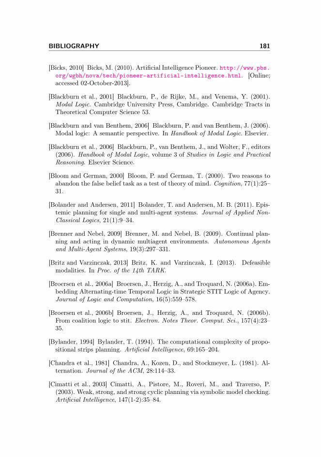
BIBLIOGRAPHY 181

[Bicks, 2010] Bicks, M. (2010). Artificial Intelligence Pioneer. http://www.pbs.org/wgbh/nova/tech/pioneer-artificial-intelligence.html. [Online;accessed 02-October-2013].

[Blackburn et al., 2001] Blackburn, P., de Rijke, M., and Venema, Y. (2001).Modal Logic. Cambridge University Press, Cambridge. Cambridge Tracts inTheoretical Computer Science 53.

[Blackburn and van Benthem, 2006] Blackburn, P. and van Benthem, J. (2006).Modal logic: A semantic perspective. In Handbook of Modal Logic. Elsevier.

[Blackburn et al., 2006] Blackburn, P., van Benthem, J., and Wolter, F., editors(2006). Handbook of Modal Logic, volume 3 of Studies in Logic and PracticalReasoning. Elsevier Science.

[Bloom and German, 2000] Bloom, P. and German, T. (2000). Two reasons toabandon the false belief task as a test of theory of mind. Cognition, 77(1):25–31.

[Bolander and Andersen, 2011] Bolander, T. and Andersen, M. B. (2011). Epis-temic planning for single and multi-agent systems. Journal of Applied Non-Classical Logics, 21(1):9–34.

[Brenner and Nebel, 2009] Brenner, M. and Nebel, B. (2009). Continual plan-ning and acting in dynamic multiagent environments. Autonomous Agentsand Multi-Agent Systems, 19(3):297–331.

[Britz and Varzinczak, 2013] Britz, K. and Varzinczak, I. (2013). Defeasiblemodalities. In Proc. of the 14th TARK.

[Broersen et al., 2006a] Broersen, J., Herzig, A., and Troquard, N. (2006a). Em-bedding Alternating-time Temporal Logic in Strategic STIT Logic of Agency.Journal of Logic and Computation, 16(5):559–578.

[Broersen et al., 2006b] Broersen, J., Herzig, A., and Troquard, N. (2006b).From coalition logic to stit. Electron. Notes Theor. Comput. Sci., 157(4):23–35.

[Bylander, 1994] Bylander, T. (1994). The computational complexity of propo-sitional strips planning. Artificial Intelligence, 69:165–204.

[Chandra et al., 1981] Chandra, A., Kozen, D., and Stockmeyer, L. (1981). Al-ternation. Journal of the ACM, 28:114–33.

[Cimatti et al., 2003] Cimatti, A., Pistore, M., Roveri, M., and Traverso, P.(2003). Weak, strong, and strong cyclic planning via symbolic model checking.Artificial Intelligence, 147(1-2):35–84.

182 BIBLIOGRAPHY

[Condon, 1992] Condon, A. (1992). The complexity of stochastic games. Infor-mation and Computation, 96:203–224.

[de Lima, 2007] de Lima, T. (2007). Optimal Methods for Reasoning about Ac-tions and Plans in Multi-Agents Systems. PhD thesis, IRIT, University ofToulouse 3, France.

[Demey, 2011] Demey, L. (2011). Some remarks on the model theory of epis-temic plausibility models. Journal of Applied Non-Classical Logics, 21(3-4):375–395.

[Ditmarsch et al., 2007] Ditmarsch, H. v., van der Hoek, W., and Kooi, B.(2007). Dynamic Epistemic Logic. Springer.

[Fagin et al., 1995] Fagin, R., Halpern, J., Moses, Y., and Vardi, M. (1995).Reasoning about Knowledge. MIT Press, Cambridge MA.

[Fikes and Nilsson, 1971] Fikes, R. E. and Nilsson, N. J. (1971). Strips: A newapproach to the application of theorem proving to problem solving. In Pro-ceedings of the 2Nd International Joint Conference on Artificial Intelligence,IJCAI’71, pages 608–620, San Francisco, CA, USA. Morgan Kaufmann Pub-lishers Inc.

[Garey and Johnson, 1979] Garey, M. R. and Johnson, D. S. (1979). Comput-ers and Intractability: A Guide to the Theory of NP-Completeness. W. H.Freeman & Co., New York, NY, USA.

[Ghallab et al., 1998] Ghallab, M., Howe, A., Knoblock, C., Mcdermott, D.,Ram, A., Veloso, M., Weld, D., andWilkins, D. (1998). PDDL—The PlanningDomain Definition Language.

[Ghallab et al., 2004] Ghallab, M., Nau, D. S., and Traverso, P. (2004). Auto-mated Planning: Theory and Practice. Morgan Kaufmann.

[Goranko and Jamroga, 2004] Goranko, V. and Jamroga, W. (2004). Compar-ing semantics of logics for multi-agent systems. SYNTHESE, 139(2):241–280.

[Grove, 1988] Grove, A. (1988). Two modellings for theory change. Journal ofPhilosophical Logic, 17:157–170.

[Haslum and Jonsson, 1999] Haslum, P. and Jonsson, P. (1999). Some resultson the complexity of planning with incomplete information. In Biundo, S. andFox, M., editors, ECP, volume 1809 of Lecture Notes in Computer Science,pages 308–318. Springer.

[Helmert, 2006] Helmert, M. (2006). The fast downward planning system. Jour-nal of Artificial Intelligence Research, 26:191–246.

BIBLIOGRAPHY 183

[Herzig et al., 2003] Herzig, A., Lang, J., and Marquis, P. (2003). Action repre-sentation and partially observable planning using epistemic logic. In Gottlob,G. and Walsh, T., editors, IJCAI, pages 1067–1072. Morgan Kaufmann.

[Herzig and Lorini, 2010] Herzig, A. and Lorini, E. (2010). A dynamic logicof agency i: Stit, capabilities and powers. Journal of Logic, Language andInformation, 19(1):89–121.

[Hintikka, 1962] Hintikka, J. (1962). Knowledge and Belief. Cornell UniversityPress, Ithaca, NY.

[Horrocks et al., 2006] Horrocks, I., Hustadt, U., Sattler, U., and Schmidt, R.(2006). Computational modal logic. In Handbook of Modal Logic. Elsevier.

[JAMES, 2014] JAMES (2014). http://homepages.inf.ed.ac.uk/rpetrick/projects/james/. [Online; accessed 12-January-2014].

[Jamroga and Ågotnes, 2007] Jamroga, W. and Ågotnes, T. (2007). Construc-tive knowledge: what agents can achieve under imperfect information. Journalof Applied Non-Classical Logics, 17(4):423–475.

[Jensen, 2013a] Jensen, M. H. (2013a). The computational complexity of singleagent epistemic planning (manuscript).

[Jensen, 2013b] Jensen, M. H. (2013b). Planning using dynamic epistemic logic:Correspondence and complexity. In Grossi, D., Roy, O., and Huang, H.,editors, LORI, volume 8196 of Lecture Notes in Computer Science, pages316–320. Springer.

[Kraus et al., 1990] Kraus, S., Lehmann, D., and Magidor, M. (1990). Non-monotonic reasoning, preferential models and cumulative logics. ArtificialIntelligence, 44:167–207.

[Lang and Zanuttini, 2013] Lang, J. and Zanuttini, B. (2013). Knowledge-basedprograms as plans: Succinctness and the complexity of plan existence. in Proc.TARK 2013.

[Laverny and Lang, 2004] Laverny, N. and Lang, J. (2004). From knowledge-based programs to graded belief-based programs part i: On-line reasoning. Inde Mántaras, R. L. and Saitta, L., editors, ECAI, pages 368–372. IOS Press.

[Laverny and Lang, 2005] Laverny, N. and Lang, J. (2005). From knowledge-based programs to graded belief-based programs, part ii: off-line reasoning. InKaelbling, L. P. and Saffiotti, A., editors, IJCAI, pages 497–502. ProfessionalBook Center.

[Lewis, 1973] Lewis, D. (1973). Counterfactuals. Harvard University Press,Cambridge (MA).

184 BIBLIOGRAPHY

[Littman, 1997] Littman, M. L. (1997). Probabilistic propositional planning:Representations and complexity. In Proceedings of the Fourteenth NationalConference on Artificial Intelligence and Ninth Conference on Innovative Ap-plications of Artificial Intelligence, AAAI’97/IAAI’97, pages 748–754. AAAIPress.

[Löwe et al., 2011] Löwe, B., Pacuit, E., and Witzel, A. (2011). Del planningand some tractable cases. In Proceedings of the Third International Confer-ence on Logic, Rationality, and Interaction, LORI’11, pages 179–192, Berlin,Heidelberg. Springer-Verlag.

[Meyer et al., 2000] Meyer, T., Labuschagne, W., and Heidema, J. (2000). Re-fined epistemic entrenchment. Journal of Logic, Language, and Information,9:237–259.

[Pacuit, 2007] Pacuit, E. (2007). Some comments on history based structures.J. Applied Logic, 5(4):613–624.

[Parikh and Ramanujam, 2003] Parikh, R. and Ramanujam, R. (2003). Aknowledge based semantics of messages. Journal of Logic, Language andInformation, 12:453–467.

[Pauly, 2002] Pauly, M. (2002). A modal logic for coalitional power in games.Journal of Logic and Computation, 12(1):149–166.

[Petrick and Bacchus, 2002] Petrick, R. P. A. and Bacchus, F. (2002). Aknowledge-based approach to planning with incomplete information and sens-ing. In Ghallab, M., Hertzberg, J., and Traverso, P., editors, AIPS, pages212–222. AAAI.

[Petrick and Bacchus, 2004] Petrick, R. P. A. and Bacchus, F. (2004). Extend-ing the knowledge-based approach to planning with incomplete informationand sensing. In [Zilberstein et al., 2004], pages 2–11.

[Premack and Woodruff, 1978] Premack, D. and Woodruff, G. (1978). Doesthe chimpanzee have a ‘theory of mind’? Behavioral and Brain Sciences,4:515–526.

[Rintanen, 2004] Rintanen, J. (2004). Complexity of planning with partial ob-servability. In [Zilberstein et al., 2004], pages 345–354.

[Rintanen, 2005] Rintanen, J. (2005). Automated planning: Algorithms andcomplexity. Habilitation thesis, Albert-Ludwigs-Universität Freiburg.

[Schwarzentruber and Herzig, 2008] Schwarzentruber, F. and Herzig, A. (2008).Properties of logics of individual and group agency. Advances in Modal Logic2006, 7:133–149.

BIBLIOGRAPHY 185

[Segerberg, 1998] Segerberg, K. (1998). Irrevocable belief revision in dynamicdoxastic logic. Notre Dame Journal of Formal Logic, 39(3):287–306.

[Sipser, 2006] Sipser, M. (2006). Introduction to the theory of computation.Thomson Course Technology, Boston, Massachusetts, 2 edition.

[Spohn, 1988] Spohn, W. (1988). Ordinal conditional functions: a dynamictheory of epistemic states. In Harper, W. and Skyrms, B., editors, Causationin Decision, Belief Change, and Statistics, volume II, pages 105–134.

[Stalnaker, 1996] Stalnaker, R. (1996). Knowledge, belief and counterfactualreasoning in games. Economics and Philosophy, 12:133–163.

[van Benthem, 1998] van Benthem, J. (1998). Dynamic odds and ends. Tech-nical Report ML-1998-08, University of Amsterdam.

[van Benthem, 2001] van Benthem, J. (2001). Games in dynamic-epistemiclogic. Bulletin of Economic Research, 53(4):219–48.

[van Benthem, 2007] van Benthem, J. (2007). Dynamic logic of belief revision.Journal of Applied Non-Classical Logics, 17(2):129–155.

[van Benthem, 2011] van Benthem, J. (2011). Logical Dynamics of Informationand Interaction. Cambridge University Press.

[van Benthem et al., 2007] van Benthem, J., Gerbrandy, J., and Pacuit, E.(2007). Merging frameworks for interaction: Del and etl. In Proceedingsof the 11th conference on Theoretical aspects of rationality and knowledge,TARK ’07, pages 72–81, New York, NY, USA. ACM.

[van der Hoek and Wooldridge, 2002] van der Hoek, W. and Wooldridge, M.(2002). Tractable multiagent planning for epistemic goals. In Proc. of theFirst International Joint Conference on Autonomous Agents & MultiagentSystems (AAMAS 2002), pages 1167–1174. ACM.

[van Ditmarsch, 2005] van Ditmarsch, H. (2005). Prolegomena to dynamic logicfor belief revision. Synthese (Knowledge, Rationality & Action), 147:229–275.

[van Ditmarsch, pear] van Ditmarsch, H. (2013, to appear). Revocable beliefrevision. Studia Logica.

[van Ditmarsch and Kooi, 2008] van Ditmarsch, H. and Kooi, B. (2008). Se-mantic results for ontic and epistemic change. In Bonanno, G., van der Hoek,W., and Wooldridge, M., editors, Logic and the Foundations of Game andDecision Theory (LOFT 7), Texts in Logic and Games, pages 87–117. Ams-terdam University Press.

186 BIBLIOGRAPHY

[van Ditmarsch and Labuschagne, 2007] van Ditmarsch, H. and Labuschagne,W. (2007). My beliefs about your beliefs – a case study in theory of mindand epistemic logic. Synthese, 155:191–209.

[van Ditmarsch et al., 2007] van Ditmarsch, H., van der Hoek, W., and Kooi,B. (2007). Dynamic Epistemic Logic. Springer Publishing Company, Incor-porated, 1st edition.

[Yu et al., 2013] Yu, Q., Wen, X., and Liu, Y. (2013). Multi-agent epistemicexplanatory diagnosis via reasoning about actions. In Rossi, F., editor, IJCAI.IJCAI/AAAI.

[Zilberstein et al., 2004] Zilberstein, S., Koehler, J., and Koenig, S., editors(2004). Proceedings of the Fourteenth International Conference on AutomatedPlanning and Scheduling (ICAPS 2004), June 3-7 2004, Whistler, BritishColumbia, Canada. AAAI.