The Application of Microeconomics to theDesign of Resource Allocation and

Control Algorithms

Donald Francis Ferguson

Submitted in partial fulfillment of therequirements for the degree

of Doctor of Philosophyin the Graduate School of Arts and Sciences

COLUMBIA UNIVERSITY1989

1989Donald Francis Ferguson

ALL RIGHTS RESERVED

ABSTRACT

The Application of Microeconomics to the Designof Resource Allocation and Control Algorithms

Donald Francis Ferguson

In this thesis, we present a new methodology for resource sharing algorithms in distributed systems.

We propose that a distributed computing system should be composed of a decentralized community

of microeconomic agents. We show that this approach decreases complexity and can substantially

improve performance. We compare the performance, generality and complexity of our algorithms

with non-economic algorithms. To validate the usefulness of our approach, we present economies

that solve three distinct resource management problems encountered in large, distributed systems.

The first economy performs CPU load balancing and demonstrates how our approach limits com-

plexity and effectively allocates resources when compared to non-economic algorithms. We show

that the economy achieves better performance than a representative non-economic algorithm. The

load balancing economy spans a broad spectrum of possible load balancing strategies, making it

possible to adapt the load balancing strategy to the relative power of CPU vs. communication.

The second economy implements flow control in virtual circuit based computer networks. This

economy implements a general model of VC throughput and delay goals that more accurately de-

scribes the goals of a diverse set of users. We propose Pareto-optimality as a definition of optimality

and fairness for the flow control problem and prove that the resource allocations computed by the

economy are Pareto-optimal. Finally, we present a set of distributed algorithms that rapidly com-

pute a Pareto-optimal allocation of resources.

The final economy manages replicated, distributed data in a distributed computer system. This

economy substantially decreases mean transaction response time by adapting to to the transactions′

reference patterns. The economy reacts to localities in the data access pattern by dynamically as-

signing copies of data objects to nodes in the system. The number of copies of each object is ad-

justed based on the write frequency versus the read frequency for the object. Unlike previous work,

the data management economy′s algorithms are completely decentralized and have low computa-

tional overhead. Finally, this economy demonstrates how an economy can allocate logical re-

sources in addition to physical resources.

Table of Contents

1.0 Introduction . . . . . . . . . . . . . . . . . . . . . . . . . . . . . . . . . . . . . . . . . . . . . . . . . . . . . . . . 11.1 The Problem . . . . . . . . . . . . . . . . . . . . . . . . . . . . . . . . . . . . . . . . . . . . . . . . . . . . . . . 11.2 The Solution . . . . . . . . . . . . . . . . . . . . . . . . . . . . . . . . . . . . . . . . . . . . . . . . . . . . . . . 41.3 Goals of the Dissertation . . . . . . . . . . . . . . . . . . . . . . . . . . . . . . . . . . . . . . . . . . . . . . . 61.4 Dissertation Overview . . . . . . . . . . . . . . . . . . . . . . . . . . . . . . . . . . . . . . . . . . . . . . . . . 7

2.0 Economic Concepts and Related Work . . . . . . . . . . . . . . . . . . . . . . . . . . . . . . . . . . . . 102.1 Economic Concepts and Terminology . . . . . . . . . . . . . . . . . . . . . . . . . . . . . . . . . . . . 10

2.1.1 Resources and Agents . . . . . . . . . . . . . . . . . . . . . . . . . . . . . . . . . . . . . . . . . . . . . 102.1.2 Prices, Budgets and Demand . . . . . . . . . . . . . . . . . . . . . . . . . . . . . . . . . . . . . . . . 112.1.3 Pareto-Optimality and Fairness . . . . . . . . . . . . . . . . . . . . . . . . . . . . . . . . . . . . . . 162.1.4 Pricing Policies . . . . . . . . . . . . . . . . . . . . . . . . . . . . . . . . . . . . . . . . . . . . . . . . . . 19

2.1.4.1 Tatonement . . . . . . . . . . . . . . . . . . . . . . . . . . . . . . . . . . . . . . . . . . . . . . . . . 192.1.4.2 Auctions . . . . . . . . . . . . . . . . . . . . . . . . . . . . . . . . . . . . . . . . . . . . . . . . . . . . 202.1.4.3 Variable Supply Models . . . . . . . . . . . . . . . . . . . . . . . . . . . . . . . . . . . . . . . . 22

2.2 Related Work . . . . . . . . . . . . . . . . . . . . . . . . . . . . . . . . . . . . . . . . . . . . . . . . . . . . . . 232.2.1 The File Allocation Problem . . . . . . . . . . . . . . . . . . . . . . . . . . . . . . . . . . . . . . . . 252.2.2 Job and Task Allocation . . . . . . . . . . . . . . . . . . . . . . . . . . . . . . . . . . . . . . . . . . . 302.2.3 Flow Control . . . . . . . . . . . . . . . . . . . . . . . . . . . . . . . . . . . . . . . . . . . . . . . . . . . 342.2.4 Multiple Access Protocols . . . . . . . . . . . . . . . . . . . . . . . . . . . . . . . . . . . . . . . . . . 39

3.0 The Load Balancing Economy . . . . . . . . . . . . . . . . . . . . . . . . . . . . . . . . . . . . . . . . . . 443.1 Problem Statement and System Model . . . . . . . . . . . . . . . . . . . . . . . . . . . . . . . . . . . . 443.2 The Economy . . . . . . . . . . . . . . . . . . . . . . . . . . . . . . . . . . . . . . . . . . . . . . . . . . . . . . 45

3.2.1 The Jobs . . . . . . . . . . . . . . . . . . . . . . . . . . . . . . . . . . . . . . . . . . . . . . . . . . . . . . 463.2.1.1 Compute the Budget Set . . . . . . . . . . . . . . . . . . . . . . . . . . . . . . . . . . . . . . . . 463.2.1.2 Computing Preferences . . . . . . . . . . . . . . . . . . . . . . . . . . . . . . . . . . . . . . . . . 463.2.1.3 Bid Generation . . . . . . . . . . . . . . . . . . . . . . . . . . . . . . . . . . . . . . . . . . . . . . . 48

3.2.2 Processors . . . . . . . . . . . . . . . . . . . . . . . . . . . . . . . . . . . . . . . . . . . . . . . . . . . . . 483.2.2.1 Auction Resources . . . . . . . . . . . . . . . . . . . . . . . . . . . . . . . . . . . . . . . . . . . . 493.2.2.2 Price Updates . . . . . . . . . . . . . . . . . . . . . . . . . . . . . . . . . . . . . . . . . . . . . . . . 493.2.2.3 Advertising . . . . . . . . . . . . . . . . . . . . . . . . . . . . . . . . . . . . . . . . . . . . . . . . . . 49

3.3 Performance Experiments . . . . . . . . . . . . . . . . . . . . . . . . . . . . . . . . . . . . . . . . . . . . . 493.3.1 Job Waiting Time . . . . . . . . . . . . . . . . . . . . . . . . . . . . . . . . . . . . . . . . . . . . . . . . 503.3.2 Spectrum of Load Balancing Strategies . . . . . . . . . . . . . . . . . . . . . . . . . . . . . . . . . 523.3.3 Adapting to CPU vs. Communication . . . . . . . . . . . . . . . . . . . . . . . . . . . . . . . . . 563.3.4 Flow Control . . . . . . . . . . . . . . . . . . . . . . . . . . . . . . . . . . . . . . . . . . . . . . . . . . . 613.3.5 Wealth, Priority and Learning . . . . . . . . . . . . . . . . . . . . . . . . . . . . . . . . . . . . . . . 62

3.4 Comparison with Related Work . . . . . . . . . . . . . . . . . . . . . . . . . . . . . . . . . . . . . . . . . 653.5 Summary . . . . . . . . . . . . . . . . . . . . . . . . . . . . . . . . . . . . . . . . . . . . . . . . . . . . . . . . . 693.6 Appendix . . . . . . . . . . . . . . . . . . . . . . . . . . . . . . . . . . . . . . . . . . . . . . . . . . . . . . . . . 70

3.6.1 Issues . . . . . . . . . . . . . . . . . . . . . . . . . . . . . . . . . . . . . . . . . . . . . . . . . . . . . . . . . 703.6.1.1 Knowledge of Resource Demands . . . . . . . . . . . . . . . . . . . . . . . . . . . . . . . . . 703.6.1.2 Auctions . . . . . . . . . . . . . . . . . . . . . . . . . . . . . . . . . . . . . . . . . . . . . . . . . . . . 703.6.1.3 Advertisements . . . . . . . . . . . . . . . . . . . . . . . . . . . . . . . . . . . . . . . . . . . . . . . 713.6.1.4 Price Guarantees . . . . . . . . . . . . . . . . . . . . . . . . . . . . . . . . . . . . . . . . . . . . . . 713.6.1.5 Flow Control . . . . . . . . . . . . . . . . . . . . . . . . . . . . . . . . . . . . . . . . . . . . . . . . 723.6.1.6 Returning Jobs . . . . . . . . . . . . . . . . . . . . . . . . . . . . . . . . . . . . . . . . . . . . . . . 72

3.6.2 The Hop 1 Algorithm . . . . . . . . . . . . . . . . . . . . . . . . . . . . . . . . . . . . . . . . . . . . . 73

4.0 The Flow Control Economy . . . . . . . . . . . . . . . . . . . . . . . . . . . . . . . . . . . . . . . . . . . . 764.1 Network and Economy . . . . . . . . . . . . . . . . . . . . . . . . . . . . . . . . . . . . . . . . . . . . . . . 76

4.1.1 Computing the Demand Set . . . . . . . . . . . . . . . . . . . . . . . . . . . . . . . . . . . . . . . . 794.1.2 Competitive Equilibrium and Price Updates . . . . . . . . . . . . . . . . . . . . . . . . . . . . . 81

4.2 Optimality and Fairness . . . . . . . . . . . . . . . . . . . . . . . . . . . . . . . . . . . . . . . . . . . . . . . 834.3 Existence of Equilibrium . . . . . . . . . . . . . . . . . . . . . . . . . . . . . . . . . . . . . . . . . . . . . . 894.4 Convergence to Equilibrium . . . . . . . . . . . . . . . . . . . . . . . . . . . . . . . . . . . . . . . . . . . 95

4.4.1 Network Updates . . . . . . . . . . . . . . . . . . . . . . . . . . . . . . . . . . . . . . . . . . . . . . . 1014.5 Comparison with Related Work . . . . . . . . . . . . . . . . . . . . . . . . . . . . . . . . . . . . . . . . 1024.6 Conclusions . . . . . . . . . . . . . . . . . . . . . . . . . . . . . . . . . . . . . . . . . . . . . . . . . . . . . . 1064.7 Proof of Lemmas . . . . . . . . . . . . . . . . . . . . . . . . . . . . . . . . . . . . . . . . . . . . . . . . . . 107

i

5.0 The Data Management Economy . . . . . . . . . . . . . . . . . . . . . . . . . . . . . . . . . . . . . . . 1165.1 Problem Statement and System Model . . . . . . . . . . . . . . . . . . . . . . . . . . . . . . . . . . . 1165.2 The Economy . . . . . . . . . . . . . . . . . . . . . . . . . . . . . . . . . . . . . . . . . . . . . . . . . . . . . 117

5.2.1 Processor Agent . . . . . . . . . . . . . . . . . . . . . . . . . . . . . . . . . . . . . . . . . . . . . . . . 1185.2.2 Data Object Agents . . . . . . . . . . . . . . . . . . . . . . . . . . . . . . . . . . . . . . . . . . . . . . 1205.2.3 Transactions . . . . . . . . . . . . . . . . . . . . . . . . . . . . . . . . . . . . . . . . . . . . . . . . . . . 121

5.3 Performance Evaluation . . . . . . . . . . . . . . . . . . . . . . . . . . . . . . . . . . . . . . . . . . . . . 1225.3.1 Ratio of Reads to Writes . . . . . . . . . . . . . . . . . . . . . . . . . . . . . . . . . . . . . . . . . . 1235.3.2 Adapting to Entropy . . . . . . . . . . . . . . . . . . . . . . . . . . . . . . . . . . . . . . . . . . . . . 1285.3.3 Adapting to Locality . . . . . . . . . . . . . . . . . . . . . . . . . . . . . . . . . . . . . . . . . . . . . 1305.3.4 Lease Prices . . . . . . . . . . . . . . . . . . . . . . . . . . . . . . . . . . . . . . . . . . . . . . . . . . . 131

5.4 Comparison with Related Work . . . . . . . . . . . . . . . . . . . . . . . . . . . . . . . . . . . . . . . . 1345.5 Conclusions . . . . . . . . . . . . . . . . . . . . . . . . . . . . . . . . . . . . . . . . . . . . . . . . . . . . . . 138

6.0 Summary and Directions for Future Work . . . . . . . . . . . . . . . . . . . . . . . . . . . . . . . . 140

Bibliography . . . . . . . . . . . . . . . . . . . . . . . . . . . . . . . . . . . . . . . . . . . . . . . . . . . . . . . . . . 143

ii

List of Illustrations

Figure 1. A Representative Distributed System . . . . . . . . . . . . . . . . . . . . . . . . . . . . . . . . . 2Figure 2. Resources . . . . . . . . . . . . . . . . . . . . . . . . . . . . . . . . . . . . . . . . . . . . . . . . . . . . 12Figure 3. A Simple Computer System . . . . . . . . . . . . . . . . . . . . . . . . . . . . . . . . . . . . . . . 13Figure 4. Auction Models . . . . . . . . . . . . . . . . . . . . . . . . . . . . . . . . . . . . . . . . . . . . . . . . 22Figure 5. Demand Functions . . . . . . . . . . . . . . . . . . . . . . . . . . . . . . . . . . . . . . . . . . . . . 24Figure 6. Demand Based Prices . . . . . . . . . . . . . . . . . . . . . . . . . . . . . . . . . . . . . . . . . . . 25Figure 7. The Contract Net Protocol . . . . . . . . . . . . . . . . . . . . . . . . . . . . . . . . . . . . . . . 32Figure 8. Multiple Access Problem . . . . . . . . . . . . . . . . . . . . . . . . . . . . . . . . . . . . . . . . . 40Figure 9. A Simple Distributed System . . . . . . . . . . . . . . . . . . . . . . . . . . . . . . . . . . . . . . 47Figure 10. A simple distributed system . . . . . . . . . . . . . . . . . . . . . . . . . . . . . . . . . . . . . . . 51Figure 11. Job Waiting Times . . . . . . . . . . . . . . . . . . . . . . . . . . . . . . . . . . . . . . . . . . . . . 52Figure 12. Job Waiting Times . . . . . . . . . . . . . . . . . . . . . . . . . . . . . . . . . . . . . . . . . . . . . 53Figure 13. Economic vs. Non-Economic Algorithms . . . . . . . . . . . . . . . . . . . . . . . . . . . . . 54Figure 14. Job Migration Distance . . . . . . . . . . . . . . . . . . . . . . . . . . . . . . . . . . . . . . . . . . 55Figure 15. Job Migration Distance . . . . . . . . . . . . . . . . . . . . . . . . . . . . . . . . . . . . . . . . . . 56Figure 16. Choice of Migration Strategy . . . . . . . . . . . . . . . . . . . . . . . . . . . . . . . . . . . . . . 57Figure 17. Communication Speed Halved . . . . . . . . . . . . . . . . . . . . . . . . . . . . . . . . . . . . . 58Figure 18. Communication Speed Doubled . . . . . . . . . . . . . . . . . . . . . . . . . . . . . . . . . . . . 59Figure 19. Migration Distances . . . . . . . . . . . . . . . . . . . . . . . . . . . . . . . . . . . . . . . . . . . . . 60Figure 20. Flow Control . . . . . . . . . . . . . . . . . . . . . . . . . . . . . . . . . . . . . . . . . . . . . . . . . 62Figure 21. Wealth as Priority . . . . . . . . . . . . . . . . . . . . . . . . . . . . . . . . . . . . . . . . . . . . . . 64Figure 22. Auctions and Prices . . . . . . . . . . . . . . . . . . . . . . . . . . . . . . . . . . . . . . . . . . . . . 65Figure 23. Price Pathology . . . . . . . . . . . . . . . . . . . . . . . . . . . . . . . . . . . . . . . . . . . . . . . . 66Figure 24. Modified HOP 1 Algorithm . . . . . . . . . . . . . . . . . . . . . . . . . . . . . . . . . . . . . . . 74Figure 25. Supply Exceeds Demand at all Prices . . . . . . . . . . . . . . . . . . . . . . . . . . . . . . . . 82Figure 26. Fairness Conditions F2 and F4 . . . . . . . . . . . . . . . . . . . . . . . . . . . . . . . . . . . . . 88Figure 27. The two dimensional example . . . . . . . . . . . . . . . . . . . . . . . . . . . . . . . . . . . . . 94Figure 28. Infinite Equilibria . . . . . . . . . . . . . . . . . . . . . . . . . . . . . . . . . . . . . . . . . . . . . . 96Figure 29. Convergence to Equilibrium Demand . . . . . . . . . . . . . . . . . . . . . . . . . . . . . . . . 97Figure 30. Convergence to Equilibrium Demand . . . . . . . . . . . . . . . . . . . . . . . . . . . . . . . . 98Figure 31. Convergence detection problem. . . . . . . . . . . . . . . . . . . . . . . . . . . . . . . . . . . . . 99Figure 32. Network Updates . . . . . . . . . . . . . . . . . . . . . . . . . . . . . . . . . . . . . . . . . . . . . 102Figure 33. Routing Pathology . . . . . . . . . . . . . . . . . . . . . . . . . . . . . . . . . . . . . . . . . . . . 103Figure 34. Strong convexity of . . . . . . . . . . . . . . . . . . . . . . . . . . . . . . . . . . . . . . . . . . . 110Figure 35. The Data Management Economy . . . . . . . . . . . . . . . . . . . . . . . . . . . . . . . . . . 119Figure 36. Data Management Distributed System . . . . . . . . . . . . . . . . . . . . . . . . . . . . . . 123Figure 37. Adapting to Read/Write Ratio . . . . . . . . . . . . . . . . . . . . . . . . . . . . . . . . . . . . 125Figure 38. Adapting to Read/Write Ratio . . . . . . . . . . . . . . . . . . . . . . . . . . . . . . . . . . . . 127Figure 39. Performance vs Entropy . . . . . . . . . . . . . . . . . . . . . . . . . . . . . . . . . . . . . . . . . 129Figure 40. Performance vs Locality of Reference . . . . . . . . . . . . . . . . . . . . . . . . . . . . . . . 131Figure 41. Adapting to Locality of Reference . . . . . . . . . . . . . . . . . . . . . . . . . . . . . . . . . 132Figure 42. Lease Prices vs Write Probability . . . . . . . . . . . . . . . . . . . . . . . . . . . . . . . . . . 133

iii

Acknowledgements

I wish to thank my advisor Yechiam Yemini for his guidance, support and friendship. I consider

myself very lucky to have had the honor and pleasure of working with him. He has had a profound

influence on this dissertation and on me. If I ever advise someone through a difficult challenge, I

will try to be like him. If I am half as good as he, I will consider myself very successful. I am looking

forward to working with him in the future.

I wish to thank my thesis committe: Zvi Galil, Michael Pinedo, Calton Pu, Mischa Schwartz and

David Simcha-levi. I think that this dissertation has benefited from their comments and my dis-

cussions with them. I also want to thank my committee for their tolerance of the many phone calls

and mail messages required to schedule the defense. I would especially like to thank Calton Pu for

the many helpful conversations with him. Seldom does one meet a person whose advice is so con-

sistently excellent.

I wish to thank the faculty, students and staff of the Computer Science Department. Despite some

trying crises, I enjoyed working with and learning from them. Special thanks go to my friends and

fellow suffering students Dannie Durand, Yoram Eisenstadter, David Glaser, Avraham Leff, Cecile

Paris, Nat Polish, Jonathan Smith, Micheal van Biema and Moti Yung. I hope my friendship has

helped them as much as their friendship helped me. I am grateful to Jed Schwartz and Alex Dupuy

for their support of the DCC projects. Many of the results in this dissertation were greatly aided

by Alex′s patience and frequent explanations of Unix and NEST. From the faculty, I give special

thanks to John Kender and Jonathan Gross. Finally, I must thank Germaine Leveque for guiding

me through the maze of forms and instructions needed to accomplish anything at Columbia. I do

not know how the department ever managed to function without her.

I have had the priveledge of working at IBM Research for most of my years in graduate school. I

have learned a great deal from this experience. I wish to thank my managers Erich Port, John

Pershing, Nagui Halim and Phil Rosenfeld for their support for my studies. I will always be

thankful for my friends′ influences on my work and on me. Special thank go to Michelle Kim (who

introduced me to IBM; little did we know), Leo Georgiadis (for his guidance through the world

on mathematics), and David Bacon (for letting me use his Suns). Finally, I must thank Christos

iv

Nikolaou who has been both an excellent advisor and a friend. He has contributed as much to this

dissertation and to me as anyone.

I want to thank Michelle Sacks for her friendship and help. I am not sure I would have made it

without her.

My in-laws Marilyn and Thomas Dente have been extremely helpful over the years. They were al-

ways there to supply encouragement, and their home was often a safe haven from the rigors of

school work.

Finally, and most importantly, I thank my wife Kim. Her confidence in me and her support kept

me going the countless times I wanted to stop. My finishing the program is as much her accom-

plishment as mine. I have not been able to be with her nearly as much as I wished and I am grateful

that I can spend the rest of my life making this up to her.

v

To Kimberly

with love

vi

1

1.0 Introduction

This dissertation focuses on the problem of allocating and sharing resources in a distributed system.

We propose a novel approach to the design of resource allocation and control algorithms in dis-

tributed systems. Our thesis is that a distributed system should be structured as an economy of

competitive microeconomic agents. Each agent independently tries to meet its individual goals, and

no attempt is made to achieve system wide performance objectives. The competition between the

agents computes a competitive equilibrium. In equilibrium, the global demand for each resource

equals the supply of the resource, and the individual agents′ demands can be satisfied. We show

how a competitive equilibrium is an optimal, fair allocation of resources.

As distributed systems increase in size and power, the complexity of making resource management

decisions grows dramatically. An important contribution of microeconomics to resource manage-

ment in distributed systems is a methodology for limiting the the complexity of solving resource

allocation problems. Our implementations of the three economies demonstrate how the new

methodology limits complexity in two ways: 1) The system is inherently modular, and 2) All de-

cision making is inherently decentralized.

To evaluate our methodology, we present three economies that solve classical resource management

problems in distributed computer systems. These are 1) load balancing [29], 2) flow control in

virtual circuit networks [9], and 3) file allocation [33]. We compare both the structure of the

economies and their performance to traditional algorithms for solving these resource management

problems.

The next section of this chapter elaborates on the complexity problems of designing resource

management algorithms in distributed computer systems. This sets the motivation for pursuing the

research presented in this dissertation. After the problems are discussed, a subsection gives an

overview of the contributions that microeconomics can make to the study of distributed systems.

Finally, the last two sections of this chapter present the main goals of this thesis, and an overview

of its research contributions.

1.1 The Problem

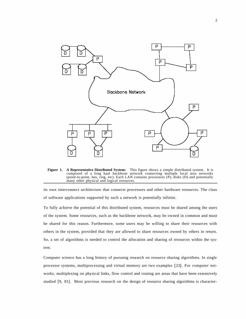
Figure 1 on page 2 shows a representative, large scale distributed system. This system is composed

of a backbone network connecting several local area networks. Each of the local area network has

2

Figure 1. A Representative Distributed System: This figure shows a simple distributed system. It iscomposed of a long haul backbone network connecting multiple local area networks(point-to-point, bus, ring, etc). Each LAN contains processors (P), disks (D) and potentiallymany other physical and logical resources.

its own interconnect architecture that connects processors and other hardware resources. The class

of software applications supported by such a network is potentially infinite.

To fully achieve the potential of this distributed system, resources must be shared among the users

of the system. Some resources, such as the backbone network, may be owned in common and must

be shared for this reason. Furthermore, some users may be willing to share their resources with

others in the system, provided that they are allowed to share resources owned by others in return.

So, a set of algorithms is needed to control the allocation and sharing of resources within the sys-

tem.

Computer science has a long history of pursuing research on resource sharing algorithms. In single

processor systems, multiprocessing and virtual memory are two examples [23]. For computer net-

works, multiplexing on physical links, flow control and routing are areas that have been extensively

studied [9, 81]. Most previous research on the design of resource sharing algorithms is character-

3

ized by at least one of two common features. The first feature is centralization. The information

needed to make a resource sharing decision is gathered in a central location, the decision is made

at this location and the result is distributed. For example, centralized algorithms for concurrency

control [8] and CPU load balancing [29] have been studied. The second feature is consensus. The

agents in the distributed system exchange information and attempt to achieve a common goal for

the system as a whole. Consensus algorithms for routing and flow control [9], concurrency control

[8] and load balancing [29] have also been proposed. For example, the common goal of a load

balancing algorithm (centralized or consensus) could be either minimizing the average response or

maximizing the total throughput.

Centralized and consensus based resource sharing algorithms attempt to compute an allocation of

resources that optimizes some system wide performance metric. This is done in the hope that im-

proving the global performance of the system will increase the ″happiness″ of the individual users.

It may be the case that the global performance objectives do not accurately represent the goals of

the diverse individual users. Defining global objectives that accurately reflect individual goals is be-

coming increasingly more difficult as the users of the system become more diverse. We show how

a competitive equilibrium is an optimal allocation with respect to the diverse, conflicting individual

goals.

As distributed systems increase in complexity, it is increasingly more difficult to design centralized

or distributed consensus algorithms that effectively allocate the resources in the system. The com-

plexity is caused by many problems. The first problem is one of scale. As the number of nodes,

resources and applications composing the system increases, centralizing information becomes im-

practical. The communication overhead incurred by centralizing the information needed to make

resource allocation decisions becomes prohibitively expensive. Furthermore, centralized decision

making does not utilize the increased computational power of a distributed, multiple processor

system.

Distributed, cooperative algorithms do not centralize information and do utilize the multiple re-

sources. However, as the size of systems increase, the rate of change of important system state in-

formation needed for resource management also increases. It may be the case that the dynamic

system state changes more rapidly than a consensus can be reached. Furthermore, the message cost

of reaching a consensus increases with the size of the system.

4

A second cause of complexity is heterogeneous users. Increased CPU power, link speeds and

memory capacity make it possible to support progressively more diverse applications in the system.

Diversity in the community of users makes it difficult to define a global performance metric that

accurately reflects the individual user goals. For example, in a database management system, the

system may try to increase throughput by increasing concurrency. The network′s goal may be low

response time of the messages it processes. The underlying operating system may be attempting to

maximize processor and memory utilization. It is not obvious that a single system goal can ade-

quately cover these three sub-goals. Furthermore, there may be conflicting goals. For example,

consider a distributed database management system supporting both simple update transactions and

complex queries [21]. The submitters of the updates might be primarily concerned with response

time, while those submitting complex queries may be concerned with throughput. It is difficult to

define a system wide goal satisfying both types of users because it is typically the case that increased

throughput causes increased response time. The same problem occurs in the network connecting

the remote users to the DBMS system. Complex queries may require shipping large amounts of

data through the network. So, throughput is important. The response time goals of the updates

imply that network delays should be minimized, which conflicts with increasing throughput. A

final problem with attempting to define a system wide goal is that the goal must be able to handle

unforeseen new applications.

Finally, both centralization and cooperation are inherently unstable. In a system using a single

processor to perform resource management decisions, a single failure can cripple the system. Co-

operative algorithms face the same problem. If even one processor fails to cooperate, or does not

cooperate as expected, the entire process can fail. Techniques such as Byzantine agreement [61] can

be used to address this problem, but at the price of increased complexity and resource requirements.

This thesis proposes using concepts drawn from microeconomics to design resource sharing algo-

rithms. In the next subsection, the new tools made available by economics are overviewed.

1.2 The Solution

Microeconomics can make two contributions to the study of resource sharing algorithms. The first

is a set of tools for limiting complexity and improving performance. The second is a set of math-

ematical models that can yield new insights into resource sharing problems.

5

Microeconomics provides three tools that can be used to limit the complexity of making resource

sharing decisions in a distributed system. The first is decentralization. The system is structured as

a set of autonomous agents, and each agent has its own goals, plans for attaining these goals and

endowment of resources that it can use. All decisions are made independently, and there is no at-

tempt to collaborate on improving the system as a whole. The second tool offered by microeco-

nomics is competition. Each agent selfishly attempts to maximize its own happiness. The agents do

not cooperate and do not attempt to reach a consensus. The third tool is the use of money, and a

price system. The price charged for a resource provides a single measure of the value of a resource

compared to all others. Money can be used to define the relative importance, or priority, of the

agents in the system. This helps deal with heterogeneity and conflicting goals.

The problems caused by scale are solved by decentralizing the decision making. When designing the

resource management algorithms, it is not necessary to take the entire system state into consider-

ation, and it is not necessary to obtain a coherent view of the system state. Instead, the algorithms′

designer simply focuses on each agent as an individual. The goal is to design algorithms that max-

imize each agents satisfaction independently of all others. The overall efficient allocation of re-

sources is the indirect result of the competition among agents. It is not intuitively obvious that

local, selfish optimization yields a globally effective allocation of resources. One of the main results

of this thesis is demonstrating that this assertion is true for problems in distributed computer sys-

tems.

Designing the system as a set of competing agents improves the system′s software structure because

the resulting algorithms are inherently modular. Agents may change their algorithms, and enter and

exit the system without necessitating changes in any other agents. This will be demonstrated with

examples in this dissertation.

Decentralization and competition also solve the problems caused by heterogeneity and diversity. It

is no longer necessary to define a common system goal that adequately reflects the wants and desires

of the diverse community. It is simply necessary to understand the goals of the individuals, and the

economic competition computes a system state that is ″optimal″ with respect to the community

of users. One of the major contributions of microeconomics is a new definition of optimality for

resource allocation in a heterogeneous distributed system: Pareto-optimality [40]. The effectiveness

of this definition is demonstrated in this dissertation.

6

Conflicting goals are resolved by competition among the agents whose goals conflict. The economy

computes a resultant state that is an equilibrium point between the conflicting goals. The resulting

state may not be optimal with respect to any individual, but is optimal with respect to the system

as a whole. The economic competition in the system determines the prices charged for resources

and services. These prices reflect the relative value of resources and provide a single measure of

value for all resources. Agents are allocated money by some policy that is external to the economy,

and this money is used to purchase the resources the agent demands. The initial endowment of

money allocated to an agent defines its priority relative to other agents. The agents simply purchase

the resources they desire at the given set of prices and use these resources as they see fit. There is

no attempt to merge disparate goals into a single system wide goal.

Finally, competition is inherently stable. The failure of agent A in an economy can only harm A

itself. Such a failure cannot cripple the system as a whole. The reliability of distributed systems

structured using microeconomics concepts is a major benefit, but it is not addressed in this disser-

tation. This dissertation focuses on the improvements in performance and system structure that are

achieved when these tools are used. Reliability of economies is a promising area of future work.

The mathematical models of microeconomics can provide new insights when computer systems are

structured as competitive economies. These models can be used to prove optimality of resource

allocations computed. It is also possible to prove the existence of an optimal equilibrium point.

In this dissertation, we demonstrate the effectiveness of these models by applying them to the flow

control problem in computer networks [9]. We also show that these models must be altered to

accurately describe the problem being studied. Additionally, we cannot make the same assumptions

as economists and it must be proven that the computer system possesses the properties typically

assumed by the economic models. This is problem is explained in chapters 2 and 4.

1.3 Goals of the Dissertation

This dissertation has the following goals:

1. To explore the similarities between complex distributed computer systems and economies:

a. To see which tools provided by economics can be applied to problems encountered in

large distributed computer systems.

2. To transform these tools into effective resource sharing algorithms and apply them to problems

in distributed computer systems.

7

a. To compare the performance of these algorithms with non-economic algorithms.

b. To determine the effects on complexity.

c. To demonstrate the broad applicability of the tools by solving diverse resource sharing

problems in distributed systems.

3. To study the applicability of mathematical economic models to distributed systems.

a. To determine the assumptions that must be changed.

1.4 Dissertation Overview

Chapter two presents the economic background for the results presented in this dissertation. This

background falls into two categories. First, we give a concise survey of the economic concepts re-

lated to the work of this dissertation, and we provide examples of the ways these concepts describe

phenomena in distributed computer systems. These examples provide further motivation for our

research. Secondly, we survey previous work on applying economic concepts to resource manage-

ment problems in distributed computer systems. We compare and contrast this previous work with

the results presented in this dissertation.

Chapter three presents the Load Balancing Economy. This economy allocates CPU resources to

jobs submitted for execution in a distributed system. Since the economy performs load balancing

across multiple processors, jobs migrate from processor to processor seeking CPU service. So, this

economy also controls the allocation of communication resources to the submitted jobs. The load

balancing economy demonstrates the applicability of decentralized decision making, competition

and a price system to a traditional problem in computer science. In this economy, the processors

selfishly attempt to maximize revenue and do not cooperate with other processors in an attempt to

minimize average response time or maximize average throughput. Similarly, the jobs in the system

compete with each other to obtain the CPU and communication resources they need to complete.

This economy demonstrates how structuring distributed systems as an economy of microeconomic

agents yields resource allocation algorithms that are inherently decentralized and modular. We will

demonstrate that both the jobs and processors can change their goals and strategies transparently

to all other agents.

The load balancing economy is extremely versatile and can easily be tuned to implement almost

any load balancing strategy. The economy spans a broad spectrum of possible load balancing

8

strategies. To evaluate the effectiveness of this economy, we compare its performance against a

representative non-economic load balancing algorithm. This comparison shows why the load bal-

ancing economy is a significant contribution to the load balancing problem independently of ex-

ploring the applicability of economics to distributed systems. Finally, we discuss the effectiveness

of wealth as a priority scheme, and the role of learning in determining the response time of indi-

vidual jobs and the average response time of the system as a whole.

Chapter four presents the Flow Control Economy. This economy allocates communication band-

width to virtual circuits in a computer network. The flow control economy illustrates the broad

applicability of microeconomics to distributed systems by solving a vastly different problem from

load balancing. The main contribution of this chapter is demonstrating the power of mathematical

economics for the description of distributed system problems and to the design of effective resource

management algorithms. Mathematical economics provides tools for proving that the resource al-

locations computed by an economy are Pareto-optimal. We prove that the algorithms of the flow

control economy compute Pareto optimal allocations of communication resources. Pareto-

optimality is a powerful definition for both optimality and fairness in heterogeneous distributed

systems. We present a formalization of fairness metrics for the flow control problem and compare

Pareto-optimality with previous definitions of fairness. Finally, we prove the existence of a

Pareto-optimal equilibrium for arbitrary networks.

Compared to previous work on flow control, the flow control economy implements a VC model

that captures the diversity of users of virtual circuits in computer networks. Under this model, each

virtual circuit′s user is able to choose an independent throughput-delay goal. We also present a set

of completely decentralized algorithm for computing optimal allocations of resources. These algo-

rithms are iterative and rapidly converge to optimal allocations.

Chapter five presents the Data Management Economy. This economy implements parts of the

Transaction Manager and Data Manager layers of a distributed data base system [8]. This chapter

demonstrates the self-tuning behavior of economies. The data management economy improves

mean transaction response time by adapting to the read/write ratio of transactions, and to localities

in transaction reference patterns. This adaptation is effective over a broad range of parameters. We

illustrate how this behavior occurs through examples. This economy also demonstrates that our

microeconomic approach can control the sharing of logical resources (access to data) as well as

physical resources. Finally, we point out some limitations of the current model.

9

Finally, chapter six is the conclusion. This chapter encapsulates the major results of the dissertation

and also discusses future avenues of research opened by the results of this thesis. These fall into two

categories. The first are direct extensions of the economies presented in this dissertation. The second

avenue branches into new areas of research. The most promising of these is generalizing math-

ematical economics so that it can be applied to a broader set of distributed computer system

models.

10

2.0 Economic Concepts and Related Work

This chapter serves two purposes. First, it contains a presentation of the economic concepts that

are used in the three economies that are the research results of this dissertation. The discussion of

economic concepts in this section is abstract. This is done so that the reader can use this section

as a starting point to applying these concepts to other distributed resource allocation problems.

The second purpose of this chapter is to provide a survey of previous work on applying economic

concepts to problems in computer science. We feel that the material in this dissertation opens new

avenues of research and compliments previous work.

The emphasis in this dissertation is on algorithms for allocating and controlling shared resources

that improve system performance. This is a very broad area of research, but it is not the only area

in which economic concepts can be used by computer science. Miller and Drexler [72] discuss other

possible contributions that the field of economics can make to computer science as a whole. This

work provides a very compelling motivation for the research in this area.

2.1 Economic Concepts and Terminology

This section provides an overview of the economic concepts and terminology used in the disserta-

tion. For more detailed presentations of this material, Hildenbrand [40], Arrow and Hahn [5] and

The Handbook of Mathematical Economics [1] are recommended. The material in this section is

drawn from these sources.

2.1.1 Resources and Agents

The major similarity between computer systems and economies is the existence of a set of resources

to be shared between multiple users. In economies, labor and coal are examples of physical re-

sources. The physical resources in a computer system could be CPU time, storage and communi-

cation bandwidth. There may are also be logical resources in both economies and computer

systems. In an economy, a patent is an example of a logical resource. In a computer system, a da-

tabase lock can be considered a logical resource.

Formally, the set of resources in an economy is denoted R1, R2, ... , RN. An allocation is a collection

or bundle of the various resources, and is a vector in • N. If x• = < x1, x2, ... , xN> i s an allocation,

then the allocation contains xi units of resource Ri. Figure 2 on page 12 depicts a simple computer

11

system with two resources. Rc represents the CPU and Rm represents main memory. An allocation

x• = < 1 0 ms, 128 Kbytes > contains 10 milliseconds of CPU time and 128 Kbytes of main memory.

In addition to resources, an economy contains a set of agents A1, A2, ... , AM, which are the active

participants in the economy. There are two types of agents in an economy. The first type is a

supplier (or producer). If agent Ai is a supplier, it controls some resources that it makes available

to be sold to the second type of agents, which are consumers. In a computer system, the operating

system (or processor) can be modeled as a supplier. It sells CPU time and memory to users of the

system, which are the consumers. Application programs and transactions are examples of con-

sumers in a computer system. The sets of suppliers and consumers are not necessarily disjoint. For

example, a database management system consumes resources (CPU, Memory) needed to perform

its functions. It also provides access to data and locks needed by user submitted transactions.

2.1.2 Prices, Budgets and Demand

A price system (or price vector) is a vector p•

in • N with pi ≥ 0. pi is the price per unit for resource

Ri. In economic theory, p•

is known by all agents. In a computer system, communication delays

may make total knowledge of p•

impossible. The agents must be robust in the face of limited

knowledge. This problem is addressed in different ways in the economies of chapters 3, 4 and 5.

Given a price system p•

it is possible to determine the cost or value of an allocation of resources x•

.

This is simply,

p•

• x• = ∑

N

i = 1

(pi • xi).

For example, in Figure 2 on page 12, if CPU time is $1 per millisecond and memory is $0.01 per

byte, then the allocation x• = < 1 0 ms, 1 Kbyte > has value (costs) $20.24. Since consumers must

purchase resources, they must be allocated some money when they enter the system. The initial

wealth, or endowment of agent Ai is denoted W i.

Given a price system and an endowment, the set of allocations agent Ai can afford is called its

budget set and is denoted

B(Ai, p• ) = {x

• p•

• x• ≤ Wi and xk ≥ 0}.

12

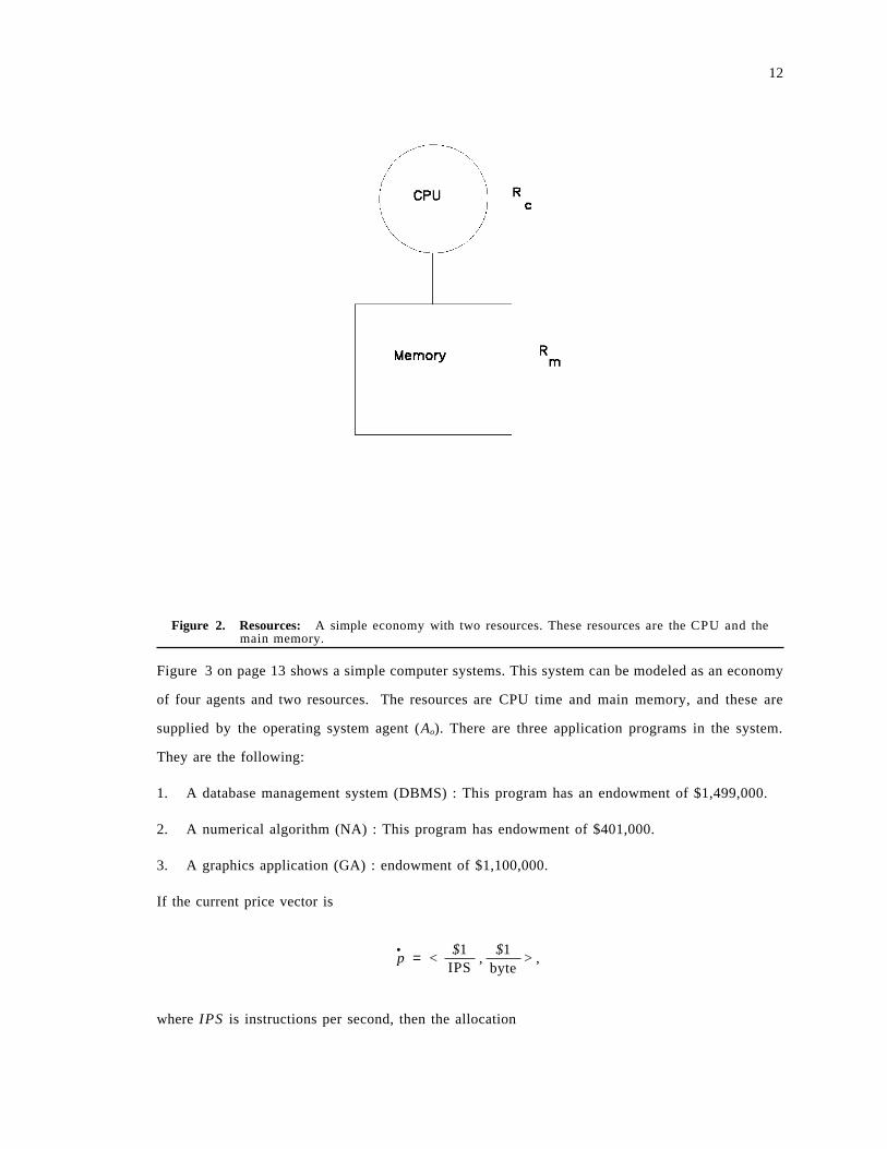
Figure 2. Resources: A simple economy with two resources. These resources are the CPU and themain memory.

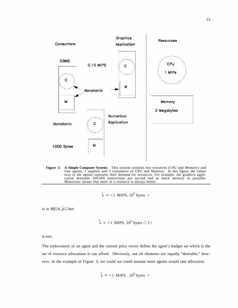
Figure 3 on page 13 shows a simple computer systems. This system can be modeled as an economy

of four agents and two resources. The resources are CPU time and main memory, and these are

supplied by the operating system agent (Ao). There are three application programs in the system.

They are the following:

1. A database management system (DBMS) : This program has an endowment of $1,499,000.

2. A numerical algorithm (NA) : This program has endowment of $401,000.

3. A graphics application (GA) : endowment of $1,100,000.

If the current price vector is

p• = <

$1IPS

,$1

byte> ,

where IPS is instructions per second, then the allocation

13

Figure 3. A Simple Computer System: This system contains two resources (CPU and Memory) andfour agents, 1 supplier and 3 consumers of CPU and Memory. In this figure, the valuesnext to the agents represent their demand for resources. For example, the graphics appli-cation demands 100,000 instructions per second and as much memory as possible.Monotonic means that more of a resource is always better.

x• = < 1 MIPS, 105 bytes >

is in B(GA , p• ), but

x• = < 1 MIPS, 105 bytes + 1 >

is not.

The endowment of an agent and the current price vector define the agent′s budget set which is the

set of resource allocations it can afford. Obviously, not all elements are equally ″desirable,″ how-

ever. In the example of Figure 3, we could we could assume most agents would rate allocation

x• = < 1 MIPS , 106 bytes >

14

less desirable than allocation

y• = <1.5 MIPS , 2 × 106 bytes > .

In an economy, each agent has a preference relation that formally defines its individual notion of

desirability. Formally, agent Ai′s preference relation is denoted • i and is a binary relation on the

set of possible allocations. If for two allocations, x• • i y

•, then Ai rates allocation x

• at least as de-

sirable as y•

. If it is not also the case that y• • i x

•, then x

• is strictly preferred to allocation y

•. Strict

preference is denoted x• • i y

•. If we have x

• • i y•

and y• • i x

•, then Ai is indifferent between x

• and

y•

. Indifference is denoted x• ∼ i y

•.

In the example of Figure 3 on page 13, assume that the numerical application requires only 103

bytes of storage to execute and needs as much CPU as possible, i.e. - the application is extremely

CPU bound. Assume that if more then 103 bytes is purchased, it will go unused. Then, for the

following three allocations:

1. x• = < 1 MIPS , 103 bytes >

2. y• = <1.5 MIPS , 103 bytes >

3. z• = < 1 MIPS , 104 bytes >

we would have

1. y• • NA x

•

2. y• • NA z

•

3. z• ∼ NA x

•

Given an agent Ai and a price system p•

, the budget set may have many elements. The agent chooses

an optimal element in B(Ai, p• ), where optimality is defined by • i. The set of optimal elements in

B(Ai, p• ) is called the demand set and is denoted Φ(Ai, p

• ). Formally,

Φ(Ai, p• ) = {x

• x• ∈ B(Ai, p

• ) and x• • i y

•, ∀y

• ∈ B(Ai, p• )}.

In the example of Figure 3 on page 13, assume that p• = < 1 , 1>. The numerical application′s de-

mand set has a single element

Φ(AN A , p• ) = {< 4 . 0 × 105 IPS , 103 bytes > }.

15

The preference relation and the endowment are key tools used to handle the diversity present in a

large, distributed system. Each agent is free to rank allocations of resources as it sees fit, and there

is no need to define a global optimal allocation. To demonstrate the modeling of diversity, we ex-

pand on the example of Figure 3 on page 13. This example will also be used in the following

sections. In the example of Figure 3 on page 13, assume that the DBMS application is interested

in maximizing throughput. Furthermore, assume that the DBMS executes 10,000 instructions and

makes 5 data references per transaction. The size of the database is 108 bytes. If a data object ref-

erenced is in the cache, then it takes an insignificant amount of time to perform the access. Oth-

erwise, 100 milliseconds are needed to fetch the object from secondary storage. Furthermore,

assume that the DBMS executes the transactions serially, and that it is suspended while an I/O is

being performed. Given these assumptions and assuming that the accesses are uniformly distrib-

uted, if x• = < x1, x2> is an allocation of resources to the DBMS, then the expected delay per

transaction is

D(x• ) = 104

x1+ (5 • 10− 1)[

(108 − x2)

(108)]

and the throughput is T(x• ) = 1

D(x• )

. In this case, for two allocations x•

and y•

, we have

x• • DBMS y

•,

if, and only if,

T(x• ) ≥ T(y• ).

The third application in this example is a graphics application. Assume that this application is

memory bound. It needs only CPU resources of 105 instructions per second, but wants as much

memory as possible. Assume that if this agent does not get 105 IPS, it cannot execute at all. Let

x•

and y•

be two allocations. This agent′s preference relation is given by the following rules:

1. If x1 < 105 and y1 < 105, then x• ∼ GA y

•. In both cases, the application cannot execute at all.

2. If x• ≥ 105 and y

• ≥ 105, then x• • GA y

•, iff x2 ≥ y2.

This example highlights two aspects of preference relations. The first is that they are very general

and can adequately model a very diverse set of resource needs in a computer system. Furthermore,

an agent′s preference relation can be defined independently of those of other agents. The second

16

aspect is that to adequately define an agent′s preference, it is necessary to understand the individual

agent′s resource usage in detail. The first aspect is a benefit, but the second can be troublesome.

For the remainder of this thesis, we assume that the resource demands of the agents are completely

known by the agents. Extending this work to other scenarios is a topic for future research.

2.1.3 Pareto-Optimality and Fairness

The goal of resource management in both economies and computer systems is to compute an

″optimal″ allocation of resources to agents. If each agent chooses its own definition of optimality,

it is not clear how to define an optimal allocation for the system as a whole. One approach to

dealing with this problem is to define a utility function for each agent, and then maximize some

function of the individual utilities. For an agent Ai, a utility function ui(x• ) is a function that maps

allocations into • with the property that x• • i y

•, if and only if, ui(x

• ) ≥ ui(y• ). In the example of

Figure 3 on page 13, T(x• ) is a utility function for the DBMS agent. For any preference relation,

it is possible to define a corresponding utility function.

Given a utility function for each agent, it is possible to define a global objective function by com-

bining the individual utilities. For example, we could maximize the sum or product of the indi-

vidual utilities. There are several problems with this strategy. First, the individual utility functions

could reflect drastically different goals. For example, u1(x• ) could be throughput for agent A1, while

u2(x• ) could be -1 times the average response time. Secondly, maximizing the sum or product of

utilities can lead to cheating. An agent may incorrectly report its utility function to obtain more

resources. Finally, maximizing global performance metrics can mean assigning 0 resources to some

agent. This is demonstrated in chapter 4.

The definition of optimality used in economics is Pareto-optimality. Intuitively, a set of allocations

φ•

1, φ•

2, ... , φ•

N of resources to agents A1, A2, ... , AN is Pareto-optimal if no agent Ai can be given a

better allocation without forcing a worse allocation on another agent. Formally, a set of allocations

φ•

1, φ•

2, ... , φ•

m to set of agents C = {A1,A2, ... , Am} is feasible if

∑i ∈ C

(φ• i

• p• ) ≤ ∑

i ∈ C

Wi.

17

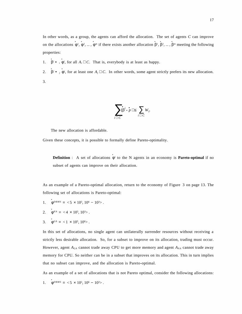
In other words, as a group, the agents can afford the allocation. The set of agents C can improve

on the allocations φ•

1, φ•

2, ... , φ•

m if there exists another allocation β•

1, β•

2, ... , β•

m meeting the following

properties:

1. β•

i • i φ•

i, for all Ai ∈ C. That is, everybody is at least as happy.

2. β•

j • j φ•

j, for at least one Aj ∈ C. In other words, some agent strictly prefers its new allocation.

3.

∑i ∈ C

(β• i

• p• ) ≤ ∑

i ∈ C

Wi.

The new allocation is affordable.

Given these concepts, it is possible to formally define Pareto-optimality.

Definition : A set of allocations φ•

i to the N agents in an economy is Pareto-optimal if no

subset of agents can improve on their allocation.

As an example of a Pareto-optimal allocation, return to the economy of Figure 3 on page 13. The

following set of allocations is Pareto-optimal:

1. φ•

D B M S = < 5 × 105, 106 − 103> .

2. φ•

N A = < 4 × 105, 103> .

3. φ•

GA = < 1 × 105, 106> .

In this set of allocations, no single agent can unilaterally surrender resources without receiving a

strictly less desirable allocation. So, for a subset to improve on its allocation, trading must occur.

However, agent AGA cannot trade away CPU to get more memory and agent AN A cannot trade away

memory for CPU. So neither can be in a subset that improves on its allocation. This in turn implies

that no subset can improve, and the allocation is Pareto-optimal.

As an example of a set of allocations that is not Pareto optimal, consider the following allocations:

1. φ•

D B M S = < 5 × 105, 106 − 103> .

18

2. φ•

N A = < 1 × 105, 5 × 105 + 103> .

3. φ•

GA = < 4 × 105, 5 × 105> .

By cooperating, agents AN A and AGA can improve on their allocations. AGA can trade 3 × 105 IPS to

agent AN A for 5 × 105 bytes of memory. This improves both agents′ allocations. Agent AGA gets the

memory necessary to execute, so it is happier. Agent AN A meets its memory requirement and re-

ceives more CPU, so it is happier.

The main advantage of Pareto optimality as a definition for optimal resource allocations is that it

does not require any coordination between the preferences or utilities of the various agents. Each

agent defines its preferences as it sees fit. This limits the complexity of the system by breaking the

resource allocation problem into N independent subproblems.

There are disadvantages to the use of Pareto-optimality as defined in the examples above. First, in

the second example, to improve on their allocations agents AN A and AGA had to barter and cooperate

to exchange resources for improving their lots. Bartering and trading are complex operations. For

example, a protocol for describing proposed trades is necessary. The second problem is that

Pareto-optimal allocations can be extremely unfair. For example, the following set of allocations

is Pareto-optimal:

1. φ•

D B M S = < 1 0 6, 2 × 106> .

2. φ•

N A = < 0 , 0 > .

3. φ•

GA = < 0 , 0 > .

Agent AD B M S cannot improve its allocation through trading, and agents AN A and AGA cannot have

their allocations improved without decreasing the desirability of AD B M S ′s allocation.

The explicit use of money in the economy eliminates these two problems. First, an agent only needs

to state its demands at the given prices. There is no need to reveal preferences and negotiate with

other agents. Secondly, Pareto-optimality together with prices implements a very rigorous definition

of fairness. For two agents Ai and Aj, the relative value of their demanded allocations at any price

system p•

will be exactly W i

W j. The agents′ endowments can be used to assign relative priority, and

the price system reflects the relative value of resources. So, each agent gets exactly it fairs share. For

example, let p = < 1 , 1 > be the current prices in the example of Figure 3 on page 13. Assume that

the following allocations are demanded:

1. φ•

D B M S = < 5 × 105, 106 − 103> .

19

2. φ•

N A = < 4 × 105, 103> .

3. φ•

GA = < 1 × 105, 106> .

We have

p•

• φ• DBMS

p•

• φ• GA

=WDBMS

WGA.

So, the relative value of the allocations demanded is exactly the same as the relative value of the

agents endowments, or priorities.

2.1.4 Pricing Policies

The previous subsections focused on the consumer agents. The main role of supplier agents is set-

ting prices. Three policies for price setting are described in this section.

2.1.4.1 Tatonement

If the demand for resource Ri at prices p•

, denoted Di(p• ), is greater than the supply Si, the resource

is undervalued and its price should be increased. If Di(p• ) < Si, then Ri is too expensive and its price

should fall. This policy for setting prices is a tatonement process, and it explicitly attempts to

compute a competitive equilibrium in which supply equals demand for all resources. A competitive

equilibrium has two desirable properties. The first is that the demand of the individual agents at the

equilibrium prices p• * can be met, and all resources are fully utilized. The second property is that the

allocation of resources in a competitive equilibrium is provably Pareto-optimal.

Define the excess demand function for resource Ri as Z i(p• ) = Di(p

• ) − Si. It is important to note that

Di(p• ) is a function of the entire price system, and not just pi. For example, consider the graphics

application AGA of Figure 3 on page 13. This application cannot execute without being allocated

105 instructions per second, and the application has WGA = $1,100,000. If the price for CPU is

greater than $11, agent AGA cannot execute and will not demand any memory. If the price for CPU

falls to $10, AGA will demand 105 IPS. This costs $1,000,000 and AGA will use the remaining $100,00

to purchase memory. So, the demand for memory will increase even if there is no change in the

price of memory.

20

Despite the fact that Di(p• ) is a function of p

• and not just pi, in the tatonement process, the supplier

of Ri only updates pi based on Z i(p• ) = Di(p

• ) − Si. The seller of Ri may not have any control over

the prices for the other resources since other agents may supply them.

The seller′s algorithm for updating pi based on Z i(p• ) is given by the formula:

pi = pi + (pi • k) • (Zi(p

• )Si

)

where k is a constant. This algorithm makes the change in price proportional to the relative differ-

ence between supply and demand, and the current price.

2.1.4.2 Auctions

The tatonement process implicitly assumes that the demand for a resources is a smooth function

of the price system p•

. This may not always be the case. For example, consider the graphics appli-

cation of Figure 3 on page 13. If the price for CPU is $11.01 per instructions per second, agent

AGA cannot afford to meet its CPU goal and will not demand any of this resource. If, however, the

price falls to $11 per IPS, agent AGA instantly demands 105 IPS. The total demand for a resource

is the sum of the individual demands. So, in this example the demand for CPU is not a smooth

function of the price system.

A second assumption for tatonement is that the resources are infinitely divisible. Memory is almost

infinitely divisible because it is composed of a very large number of very small units, each of which

can be sold separately. A lock on a record in a database is an example of a resource that is not in-

finitely divisible. The lock is either held, or not held. This is an example of a resource which is a

discrete, indivisible quantity.

If the resource is not infinitely divisible and the demand does not vary smoothly with prices, an

alternative to tatonement must be used. In this section, we discuss auction models for setting prices

and selling resources.

Assume that resource Ri comes in a fixed, discrete supply Si. This resource′s producer Pj can hold

an auction to sell Ri. Pi′s goal is to maximize revenue by selling the resource at the highest price a

consumer agent is willing to pay. The strategy of the consumers is twofold. First, a consumer Ak

that wants to purchase Ri attempts to obtain the resource at the lowest price. Ak also must consider

21

the usefulness of resource Ri relative to other resources and their prices. This determines how much

Ak is willing to pay for Ri.

There are many auction models for selling resources [24]. In this section, we briefly describe three

models. The auction models used in the load balancing economy are based on the policies described

here.

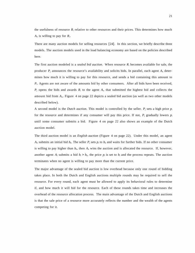
The first auction modeled is a sealed bid auction. When resource Ri becomes available for sale, the

producer Pj announces the resource′s availability and solicits bids. In parallel, each agent Ak deter-

mines how much it is willing to pay for this resource, and sends a bid containing this amount to

Pi. Agents are not aware of the amounts bid by other consumers. After all bids have been received,

Pj opens the bids and awards Ri to the agent Aw that submitted the highest bid and collects the

amount bid from Aw. Figure 4 on page 22 depicts a sealed bid auction (as well as two other models

described below).

A second model is the Dutch auction. This model is controlled by the seller. Pj sets a high price pi

for the resource and determines if any consumer will pay this price. If not, Pj gradually lowers pi

until some consumer submits a bid. Figure 4 on page 22 also shows an example of the Dutch

auction model.

The third auction model is an English auction (Figure 4 on page 22). Under this model, an agent

Ak submits an initial bid bk. The seller Pj sets pi to bk and waits for further bids. If no other consumer

is willing to pay higher than bk, then Ak wins the auction and is allocated the resource. If, however,

another agent Al submits a bid bl > bk, the price pi is set to bl and the process repeats. The auction

terminates when no agent is willing to pay more than the current price.

The major advantage of the sealed bid auction is low overhead because only one round of bidding

takes place. In both the Dutch and English auctions multiple rounds may be required to sell the

resource. For every round, each agent must be allowed to apply its behavioral rules to determine

if, and how much it will bid for the resource. Each of these rounds takes time and increases the

overhead of the resource allocation process. The main advantage of the Dutch and English auctions

is that the sale price of a resource more accurately reflects the number and the wealth of the agents

competing for it.

22

Figure 4. Auction Models: This figure represents three different auction models. In a sealed bidauction, all bids are submitted in parallel and the highest bidder wins. In a Dutch auction,the seller progressively lowers the price of the resource until a bid is submitted. Under theEnglish auction model, the consumers individually submit progressively higher bids until thehighest bidder is determined.

2.1.4.3 Variable Supply Models

The tatonement and auction models assume that the supply of each resource Ri is fixed at Si. This

is not necessarily the case, and the data management economy in chapter 5 contains resources for

which the supply can contract and expand dynamically. Since the supply can expand and contract

to match the demand, the seller can attempt to set the price pi to the value that maximizes its re-

venue. That is, the producer Pj attempt to find pi that maximizes

pi • Di(p• ).

Determining p*i that maximizes revenue is an extremely difficult task. There are two reasons for this.

First, the demand for Ri is a function of all resource prices, not just pi. Secondly, the demand

function Di(p• ) can be any arbitrary function of p

• and is not necessarily well behaved. Figure 5 on

23

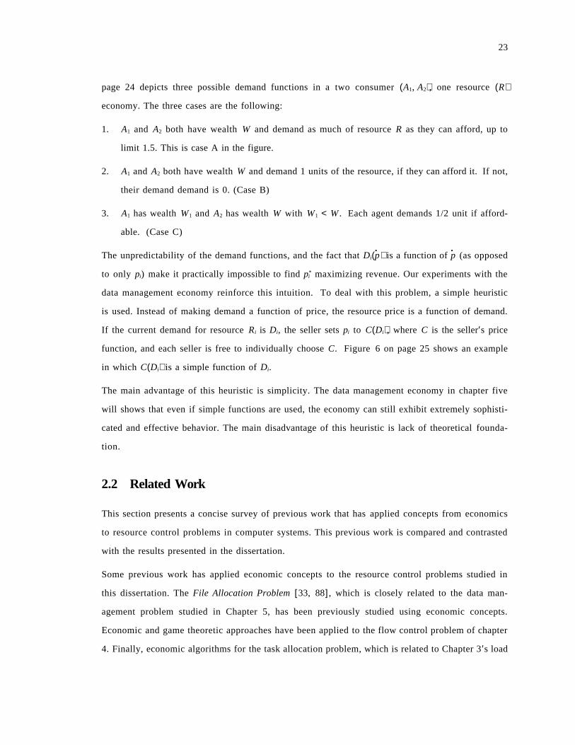
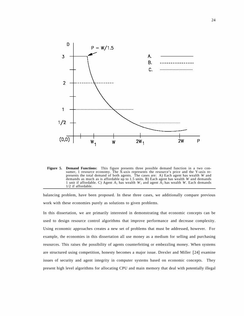
page 24 depicts three possible demand functions in a two consumer (A1, A2), one resource (R)

economy. The three cases are the following:

1. A1 and A2 both have wealth W and demand as much of resource R as they can afford, up to

limit 1.5. This is case A in the figure.

2. A1 and A2 both have wealth W and demand 1 units of the resource, if they can afford it. If not,

their demand demand is 0. (Case B)

3. A1 has wealth W1 and A2 has wealth W with W1 < W . Each agent demands 1/2 unit if afford-

able. (Case C)

The unpredictability of the demand functions, and the fact that Di(p• ) is a function of p

• (as opposed

to only pi) make it practically impossible to find p*i maximizing revenue. Our experiments with the

data management economy reinforce this intuition. To deal with this problem, a simple heuristic

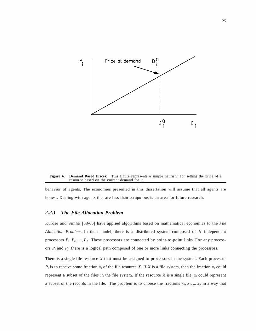
is used. Instead of making demand a function of price, the resource price is a function of demand.

If the current demand for resource Ri is Di, the seller sets pi to C(Di), where C is the seller′s price

function, and each seller is free to individually choose C. Figure 6 on page 25 shows an example

in which C(Di) is a simple function of Di.

The main advantage of this heuristic is simplicity. The data management economy in chapter five

will shows that even if simple functions are used, the economy can still exhibit extremely sophisti-

cated and effective behavior. The main disadvantage of this heuristic is lack of theoretical founda-

tion.

2.2 Related Work

This section presents a concise survey of previous work that has applied concepts from economics

to resource control problems in computer systems. This previous work is compared and contrasted

with the results presented in the dissertation.

Some previous work has applied economic concepts to the resource control problems studied in

this dissertation. The File Allocation Problem [33, 88], which is closely related to the data man-

agement problem studied in Chapter 5, has been previously studied using economic concepts.

Economic and game theoretic approaches have been applied to the flow control problem of chapter

4. Finally, economic algorithms for the task allocation problem, which is related to Chapter 3′s load

24

Figure 5. Demand Functions: This figure presents three possible demand function in a two con-sumer, 1 resource economy. The X-axis represents the resource′s price and the Y-axis re-presents the total demand of both agents. The cases are: A) Each agent has wealth W anddemands as much as is affordable up to 1.5 units. B) Each agent has wealth W and demands1 unit if affordable. C) Agent A1 has wealth W 1 and agent A2 has wealth W . Each demands1/2 if affordable.

balancing problem, have been proposed. In these three cases, we additionally compare previous

work with these economies purely as solutions to given problems.

In this dissertation, we are primarily interested in demonstrating that economic concepts can be

used to design resource control algorithms that improve performance and decrease complexity.

Using economic approaches creates a new set of problems that must be addressed, however. For

example, the economies in this dissertation all use money as a medium for selling and purchasing

resources. This raises the possibility of agents counterfeiting or embezzling money. When systems

are structured using competition, honesty becomes a major issue. Drexler and Miller [24] examine

issues of security and agent integrity in computer systems based on economic concepts. They

present high level algorithms for allocating CPU and main memory that deal with potentially illegal

25

Figure 6. Demand Based Prices: This figure represents a simple heuristic for setting the price of aresource based on the current demand for it.

behavior of agents. The economies presented in this dissertation will assume that all agents are

honest. Dealing with agents that are less than scrupulous is an area for future research.

2.2.1 The File Allocation Problem

Kurose and Simha [58-60] have applied algorithms based on mathematical economics to the File

Allocation Problem. In their model, there is a distributed system composed of N independent

processors P1, P2, ... , PN. These processors are connected by point-to-point links. For any process-

ors Pi and Pj, there is a logical path composed of one or more links connecting the processors.

There is a single file resource X that must be assigned to processors in the system. Each processor

Pi is to receive some fraction xi of the file resource X. If X is a file system, then the fraction xi could

represent a subset of the files in the file system. If the resource X is a single file, xi could represent

a subset of the records in the file. The problem is to choose the fractions x1, x2, ... xN in a way that

26

optimizes some performance measure. The xi are percentages of the total resource assigned to the

processors. So, we have

1. ∑N

i = 1

xi = 1.

2. 0 ≤ xi ≤ 1.

Accesses to the file resource are generated at all processors in the system. As a simplification, it is

assumed that the accesses are uniformly distributed over the entire file resource. So, xi is also the

probability that a file access submitted anywhere in the system will be routed to Pi for processing.

It is assumed that there is an analytic model describing the performance of the underlying distrib-

uted system. This model is used to define a function that will be optimized by the choices of the

xi. The model is defined by the following parameters:

1. λi - The rate at which file accesses are generated at Pi. This is assumed to be a poisson process.

The network wide access arrival rate is λ = ∑N

i = 1

λi.

2. c• - The communication cost of transmitting an access from Pi to Pj and returning the response

to Pi.

3. Ci - The average system wide communication cost of making an access at node Pi. This is the

weighted average over all nodes and is

Ci = ∑N

j = 1

λi

λ• cji.

4. 1µ - The average processor service time for an access request, which is exponentially distrib-

uted.

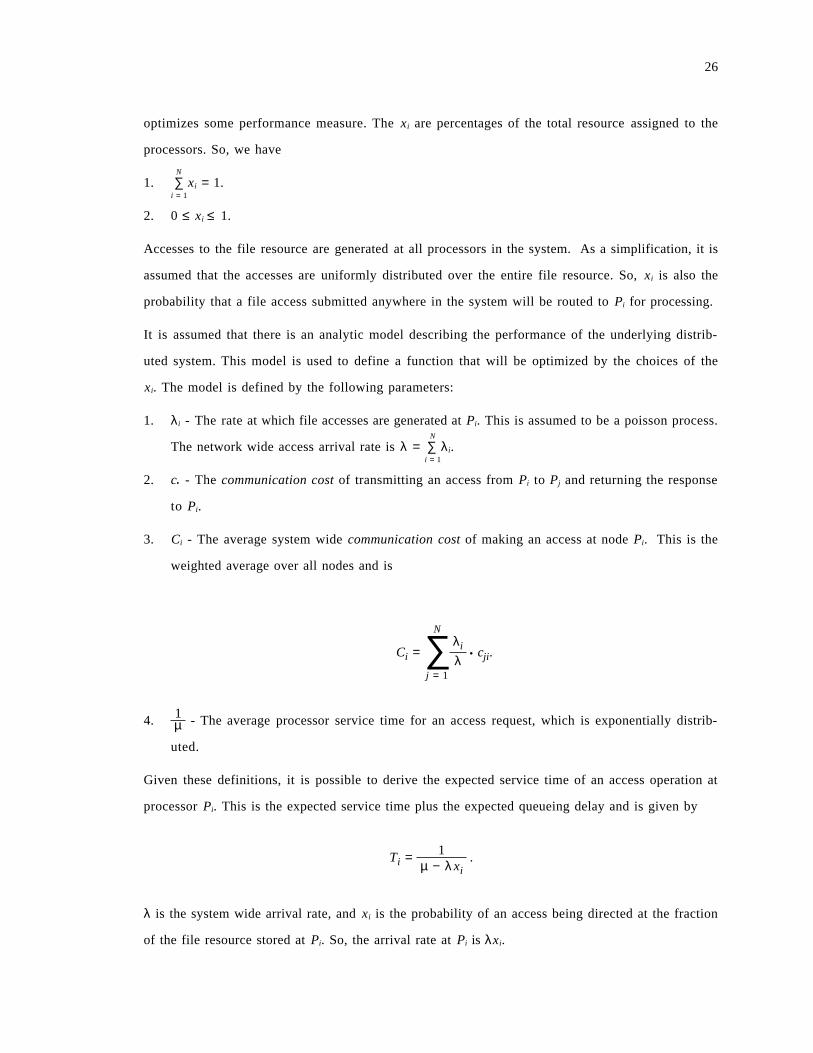
Given these definitions, it is possible to derive the expected service time of an access operation at

processor Pi. This is the expected service time plus the expected queueing delay and is given by

Ti = 1µ − λxi

.

λ is the system wide arrival rate, and xi is the probability of an access being directed at the fraction

of the file resource stored at Pi. So, the arrival rate at Pi is λxi.

27

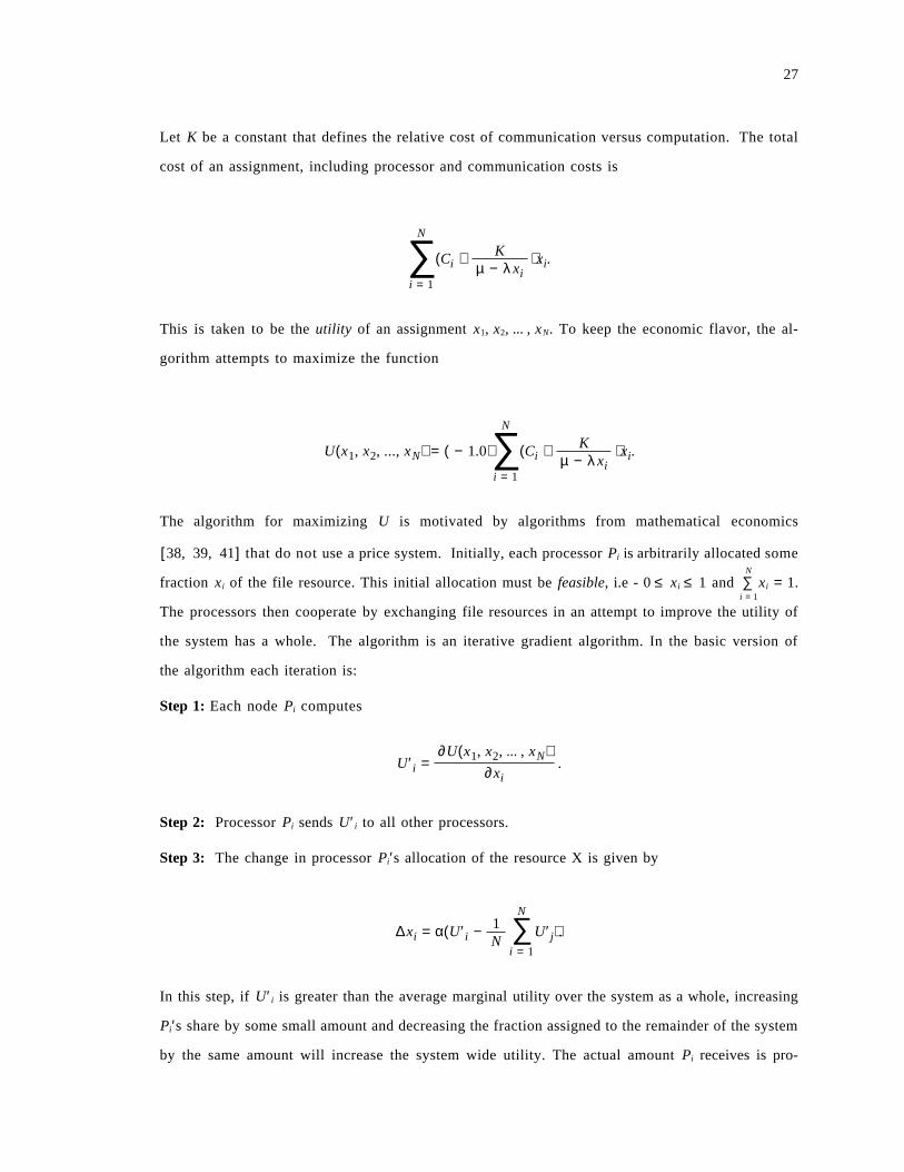
Let K be a constant that defines the relative cost of communication versus computation. The total

cost of an assignment, including processor and communication costs is

∑N

i = 1

(Ci + Kµ − λxi

)xi.

This is taken to be the utility of an assignment x1, x2, ... , xN. To keep the economic flavor, the al-

gorithm attempts to maximize the function

U(x1, x2, ..., xN) = ( − 1.0)∑N

i = 1

(Ci + Kµ − λxi

)xi.

The algorithm for maximizing U is motivated by algorithms from mathematical economics

[38, 39, 41] that do not use a price system. Initially, each processor Pi is arbitrarily allocated some

fraction xi of the file resource. This initial allocation must be feasible, i.e - 0 ≤ xi ≤ 1 and ∑N

i = 1

xi = 1.

The processors then cooperate by exchanging file resources in an attempt to improve the utility of

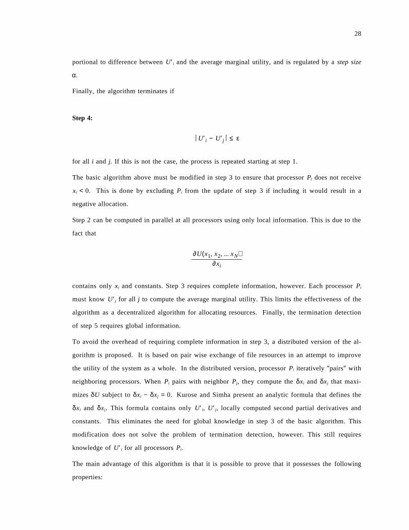
the system has a whole. The algorithm is an iterative gradient algorithm. In the basic version of

the algorithm each iteration is:

Step 1: Each node Pi computes

U′i =∂U(x1, x2, ... , xN)

∂xi.

Step 2: Processor Pi sends U′ i to all other processors.

Step 3: The change in processor Pi′s allocation of the resource X is given by

∆xi = α(U′i − 1N ∑

N

i = 1

U′j).

In this step, if U′ i is greater than the average marginal utility over the system as a whole, increasing

Pi′s share by some small amount and decreasing the fraction assigned to the remainder of the system

by the same amount will increase the system wide utility. The actual amount Pi receives is pro-

28

portional to difference between U′ i and the average marginal utility, and is regulated by a step size

α.

Finally, the algorithm terminates if

Step 4:

U′i − U′j ≤ ε

for all i and j. If this is not the case, the process is repeated starting at step 1.

The basic algorithm above must be modified in step 3 to ensure that processor Pi does not receive

xi < 0. This is done by excluding Pi from the update of step 3 if including it would result in a

negative allocation.

Step 2 can be computed in parallel at all processors using only local information. This is due to the

fact that

∂U(x1, x2, ... xN)∂xi

contains only xi and constants. Step 3 requires complete information, however. Each processor Pi

must know U′ j for all j to compute the average marginal utility. This limits the effectiveness of the

algorithm as a decentralized algorithm for allocating resources. Finally, the termination detection

of step 5 requires global information.

To avoid the overhead of requiring complete information in step 3, a distributed version of the al-

gorithm is proposed. It is based on pair wise exchange of file resources in an attempt to improve

the utility of the system as a whole. In the distributed version, processor Pi iteratively ″pairs″ with

neighboring processors. When Pi pairs with neighbor Pj, they compute the δxi and δx j that maxi-

mizes δU subject to δxi − δx j = 0. Kurose and Simha present an analytic formula that defines the

δxi and δx j. This formula contains only U′ i, U′ j, locally computed second partial derivatives and

constants. This eliminates the need for global knowledge in step 3 of the basic algorithm. This

modification does not solve the problem of termination detection, however. This still requires

knowledge of U′ i for all processors Pi.

The main advantage of this algorithm is that it is possible to prove that it possesses the following

properties:

29

1. Optimality : The algorithm computes feasible xi that maximize the utility function

U(xi, x2, ... , xN).

2. Convergence : The algorithm converges monotonically to an optimal allocation. The proof sets

an upper bound for the step size α. With this value, simulation studies showed that the algo-

rithm converges very slowly (7000 iterations). However, the algorithm converged very rapidly

for values larger than stipulated by the proof.

There are several potential problems with the model used for this algorithm. The most serious is

the assumption that the behavior of the underlying distributed system can adequately be predicted

by a simple analytic formula. These algorithms require that the analytic function be continuous and

differentiable. A second disadvantage is that termination detection requires global information.

There is also room for improvement over this algorithm. First, it assumes that the accesses are

uniformly distributed over the entire file resource. So, the algorithm does not detect and exploit

any locality in the reference patterns. For example, processor Pi may exclusively access a specific

fraction of the file resource. Kurose and Simha′s algorithm only determines the size of the file re-

source fraction to allocate to Pi and does not consider its contents. Finally, there is a single copy

of the file resource. Varying the number of copies of fractions of the file system may improve per-

formance. For example, if some fraction x 0 is exclusively read, then a copy should be assigned to

every processor. If fraction x 1 is only written, then there should be a single copy.

The data management economy of chapter 5 solves the above problems. First, no analytic model

of the underlying system is assumed. Second, in the data management economy, all decision making

is completely decentralized. Processor Pi only needs to know the read and write lease prices for a

data object oj, and the demand for access to oj experienced locally to make decisions. We will show

that the data management economy exploits locality in the access patterns to improve performance.

The economy also adjusts the number of copies of a data object to reflect the ratio of read access

to write access for the object.

The main disadvantage of the data management economy compared to the work of Kurose and

Simha is that it is not possible to prove optimality of the allocation computed. This economy is

evaluated through an implementation and simulation study.

30

2.2.2 Job and Task Allocation

Some previous work has applied economic concepts to the task, or job, allocation problem

[68, 87]. In this problem, there is a set of jobs or tasks, denoted T1, T2, ... , TN that have to be ex-

ecuted in the distributed system. The problem is to assign the tasks to processors in the system.

This assignment should fully utilize the processing power of each node in the system and must take

into consideration any special dependencies a task has on hardware or software resources that are

only available on a subset of the nodes. The object of the assignment is to optimize some per-

formance metric such as task throughput, average task response time or total elapsed time.

If the set of tasks {T1, T2, ... , TN} is static, i.e. - no new tasks arrive, the problem is a pure task al-

location problem. There may be some precedence relation between the tasks. It is usually assumed

that the inter-task communication between each pair of tasks is known. So, the assignment of tasks

to processors must also consider the communication cost incurred when Ti and T j are assigned to

different processors. In this section, we discuss the Contract Net Protocol [22, 83, 85]. This is a

protocol for the task allocation problem that has been developed using a contract and negotiation

metaphor. One of this protocol′s sub functions is based on bidding, as is the load balancing

economy of chapter 3.

If the set of tasks changes dynamically due to arrivals of new tasks and completion of others, the

problem is modeled as a load balancing problem. The Contract Net Protocol has been used as a

basis for the Distributed Scheduling Protocol of the Enterprise System [66, 67]. This protocol im-

plements a distributed, dynamic load sharing algorithm and is surveyed in this section.

The idea underlying the Contract Net Protocol is the use of negotiation between intelligent, au-

tonomous agents as a method for structuring distributed processing problems. In this model, the

system as a whole tries to solve some single problem, e.g. - the Distributed Sensing Problem

(DSP) [84] . In this problem, there is a set of processors and a set of sensing devices. The sensors

collect information and report it to processing nodes, which analyze and interpret the information

in cooperation with other processing and sensor nodes. The system as a whole attempts to com-

pute the location and motion of objects in the area covered.

Complex problems such as the Distributed Sensing Problem require that the overall problem be

broken down into separate sub problems. Each of these sub problems is a task which must be

assigned to some node in the system. The Contract Net Protocol tries to solve a generalized task

allocation problem.

31

The Contract Net Protocol starts when node Pi has a task T j that is suitable for remote execution.

Pi sends a task announcement message to other processors in the system. This message contains a

description of T j that can include estimated CPU time, memory requirements and any hardware

dependencies. Figure 7 on page 32 depicts the phases of the Contract Net Protocol. In this exam-

ple, P1 is announcing task A and P4 is announcing task B.

The recipient of a task announcement processes the message. This involves determining if the

processor is able to perform the task, e.g. - contains the necessary hardware resources. This an-

nouncement is ranked using some problem specific criteria and is queued internally. When a

processor Pj completes its current task and becomes idle, it picks the ″best″ locally queued an-

nouncement. Pj then submits a bid to the processor announcing the task (known as the manager).

The bid contains a list of Pj′s qualifications for performing the task. In the example of Figure 7 on

page 32, processors P1 and P2 bid on task B and P3 bids on task A.

The manager of an announced task waits specified time interval for bids to be submitted. After the

interval expires, all submitted bids are evaluated and the best bid is determined. The best bidder is

sent an award message telling it that it has won. This message contains any additional information

needed for the winner to process the task. The losers are sent cancel messages informing them of

their misfortune. In the Figure 7 on page 32, P3 is awarded task A and P1 is awarded task task B.

Nodes P1 and P3 are part of a contract and may exchange information on the progress of task A.

The Contract Net Protocol is proposed as a paradigm for structuring large, complex problems in

a distributed computing environment. In this protocol, all agents in the system are cooperating to

achieve a single goal. In the economies in this dissertation, the agents compete for scarce resources

and each agent attempts to meet its individual goals. The Contract Net Protocol performs resource

control in a distributed system for a different set of problems than our economies. Our economies

operate in environments where physical and logical resources are scarce, and there is competition

for these resources. The Contract Net Protocol is designed to match the logical demand for re-

sources with the agents best capable of providing these resources. This protocol does not address

environments in which there is competition for scarce resources.

The Contract Net Protocol has been used for the basis of the Distributed Scheduling Protocol of

the Enterprise System. The Enterprise system is applied to the task allocation problem in a local

area network of workstations. The goal is to utilize the capacity of idle nodes by remotely submit-

ting tasks on the idle workstations. The Enterprise System has three layers. These are: 1) An

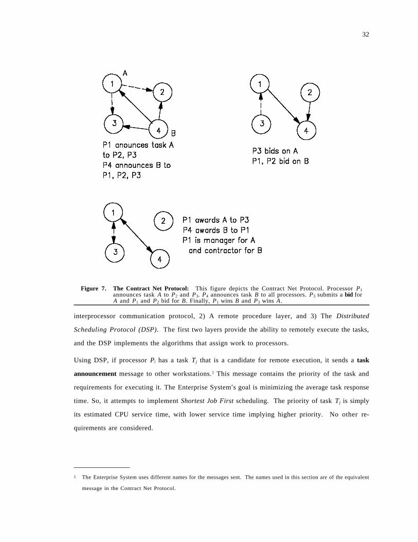
32

Figure 7. The Contract Net Protocol: This figure depicts the Contract Net Protocol. Processor P1announces task A to P2 and P3. P4 announces task B to all processors. P3 submits a bid forA and P1 and P2 bid for B. Finally, P1 wins B and P3 wins A.

interprocessor communication protocol, 2) A remote procedure layer, and 3) The Distributed

Scheduling Protocol (DSP). The first two layers provide the ability to remotely execute the tasks,

and the DSP implements the algorithms that assign work to processors.

Using DSP, if processor Pi has a task T j that is a candidate for remote execution, it sends a task

announcement message to other workstations.1 This message contains the priority of the task and

requirements for executing it. The Enterprise System′s goal is minimizing the average task response

time. So, it attempts to implement Shortest Job First scheduling. The priority of task T j is simply

its estimated CPU service time, with lower service time implying higher priority. No other re-

quirements are considered.

1 The Enterprise System uses different names for the messages sent. The names used in this section are of the equivalent

message in the Contract Net Protocol.

33

Each workstation receiving a task announcement ranks the announcement based on estimated ser-

vice time and queues it. When the processor becomes idle, it submits a bid for the highest ranked

announcement that is locally queued. The processor′s estimated service time for the task, based

on its CPU speed, is included in the bid. This is the processors qualification for executing the task.

Processor Pi waits for some time interval accumulating bids. When the interval expires, the task is

awarded to the best bidder. The winner is the processor that reports the smallest estimated service

time. An award message is sent to the winner, and the other bidders are sent cancel messages.

If processor Pi later receives a bid for task T j that is ″significantly better″ than the bid that won, Pi

can subsequently cancel the award and reassign the task to the better bidder. The definition of sig-

nificantly better is a parameter to the system.

The Enterprise System and the Distributed Scheduling Protocol were evaluated through simulation.

The main results that relate to the load balancing economy are the following:

1. Network size:

a. Significant performance improvements were achieved for relatively small networks (8-10)

nodes.

b. Marginally decreasing performance improvements occur as network size increases.

2. Communication delay : The system improves performance when the communication delay of

migrating a task is from 0 - 20% of the average CPU service demand.

3. Cancel/Reassignment : Allowing canceling and reassignment of tasks when better bids arrive

is effective at low utilizations and counter productive at higher utilizations.

4. Error in estimates : The system is very insensitive to errors in the estimated service times of the

jobs.

This dissertation′s load balancing economy and the Enterprise System pursue fundamentally dif-

ferent approaches to performing resource allocation. In the load balancing economy, a job′s pri-

ority is based on its initial endowment of money. We will show in chapter 3 that Shortest Job First

as well as other scheduling policies can be implemented by this mechanism.

The load balancing economy is based on selfish optimization and competition. Processors solely

try to maximize their individual revenue, and are not concerned with performance. The jobs

compete with each other for the scarce communication and CPU resources. The Enterprise System

34

is based on altruism, and each processor attempts to optimize the performance of the system as a

whole.

The load balancing economy implements load balancing heuristics that the Enterprise System lacks.

The Enterprise System works well over a wide range of CPU to communication ratios. It does not

adapt its behavior to this ratio, however. The Enterprise System makes the same task allocation

decisions regardless of the CPU/Communication ratio. We show in chapter 3 that the load bal-

ancing economy does modify its load balancing strategies based on the underlying communication

and CPU processing rates. We will show how this economy can be tuned to change its load bal-

ancing strategy based on the job migration cost vs. the CPU service cost. Finally, the load balancing

economy exhibits flow control. At high utilizations, poor jobs starve improving the performance

of their relatively wealth competitors.

2.2.3 Flow Control

Some previous work has applied concepts from economics to the problem of flow control in com-

puter communication networks. This previous work primarily deals with game theoretic models

for Markovian networks [51]. At the end of this survey, the main differences between the previous

work and the material of this dissertations are discussed.

In a computer communication network there is an implicit trade-off between throughput and delay.

Throughput is the rate at which users transmit data through the network. Delay is the average

elapsed time between the sending of the data and its arrival at the destination. Ideally, throughput

should be ″high″ and delay ″low.″ However, high throughput causes high delays, and decreasing

delay constrains throughput. An equilibrium point between these two conflicting goals must be

achieved.

Hsiao and Lazar [42, 43] observed the similarities between the flow control problem in a heter-

ogeneous computer network and the theory of non-cooperatives games [82]. The two main simi-

larities are:

1. Decentralization : Each user has an individual goal.

2. Competition : The users′ goals conflict. For example, increasing the throughput of user A will

increase the delay of another user B.

Hsiao and Lazar applied game theoretic concepts to describe the flow control problem for

Markovian networks. In their model, there are K classes of users, and each class is represented by

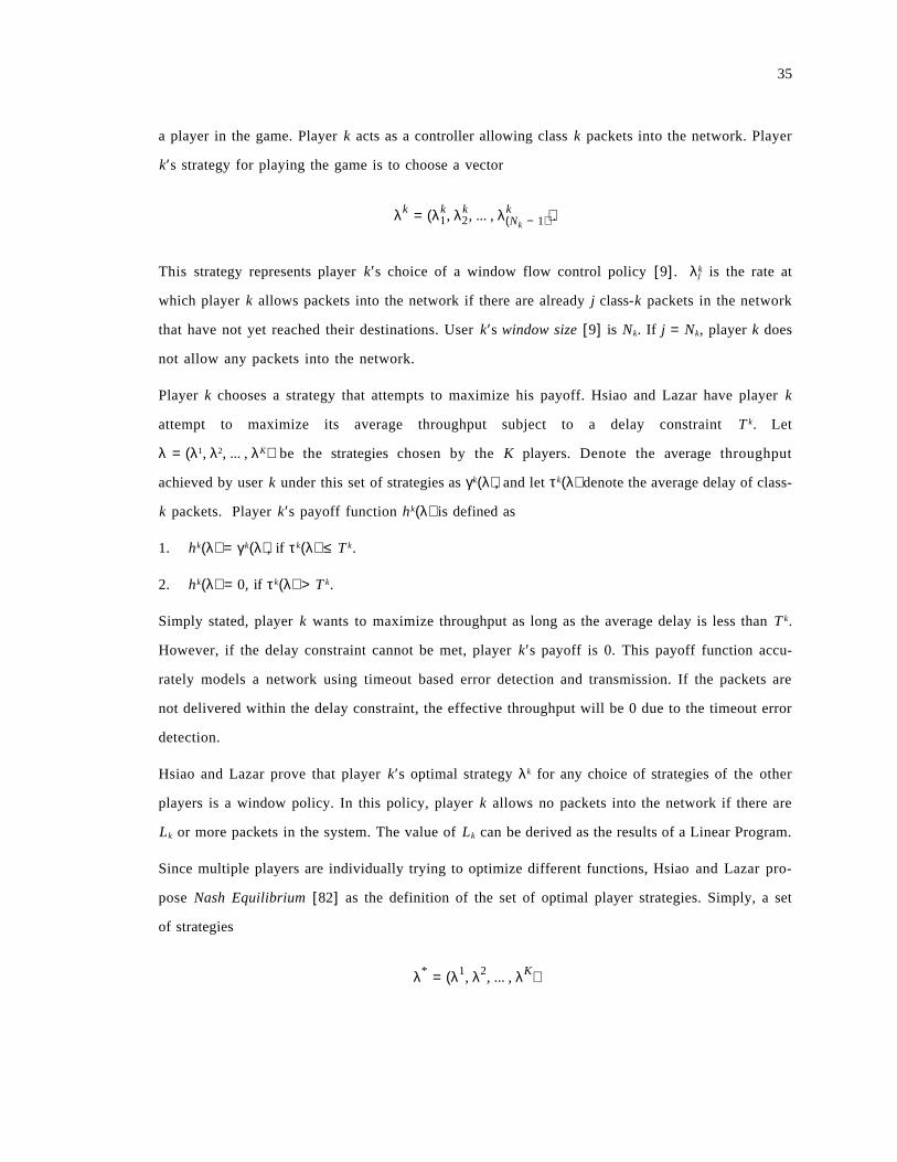
35

a player in the game. Player k acts as a controller allowing class k packets into the network. Player

k′s strategy for playing the game is to choose a vector

λk = (λk1, λk

2, ... , λk(Nk − 1)).

This strategy represents player k′s choice of a window flow control policy [9]. λkj is the rate at

which player k allows packets into the network if there are already j class-k packets in the network

that have not yet reached their destinations. User k′s window size [9] is Nk. If j = Nk, player k does

not allow any packets into the network.

Player k chooses a strategy that attempts to maximize his payoff. Hsiao and Lazar have player k

attempt to maximize its average throughput subject to a delay constraint T k. Let

λ = (λ1, λ2, ... , λK) be the strategies chosen by the K players. Denote the average throughput

achieved by user k under this set of strategies as γk(λ), and let τk(λ) denote the average delay of class-

k packets. Player k′s payoff function hk(λ) is defined as

1. hk(λ) = γ k(λ), if τk(λ) ≤ T k.

2. hk(λ) = 0, if τk(λ) > T k.

Simply stated, player k wants to maximize throughput as long as the average delay is less than T k.

However, if the delay constraint cannot be met, player k′s payoff is 0. This payoff function accu-

rately models a network using timeout based error detection and transmission. If the packets are

not delivered within the delay constraint, the effective throughput will be 0 due to the timeout error

detection.

Hsiao and Lazar prove that player k′s optimal strategy λk for any choice of strategies of the other

players is a window policy. In this policy, player k allows no packets into the network if there are

Lk or more packets in the system. The value of Lk can be derived as the results of a Linear Program.

Since multiple players are individually trying to optimize different functions, Hsiao and Lazar pro-

pose Nash Equilibrium [82] as the definition of the set of optimal player strategies. Simply, a set

of strategies

λ* = (λ1, λ2, ... , λK)

36

is a Nash Equilibrium if no player can achieve a higher payoff (i.e. - More throughput without

violating delay constraints) by unilaterally changing its strategy. Hsiao and Lazar then derive the

set of flow control problems for which the Nash Equilibrium exists.

Bovopoulos and Lazar [11] expand on the work of Hsiao and Lazar by presenting algorithms for

computing a Nash Equilibrium under two different network models. In the first model, each player

has the payoff function described above. There are only two players in the game, however. The first

algorithm is as follows:

Step 1: Start with an initially empty network, with λ1 = λ2 = 0.

Step 2: Player 1 chooses λ1 that maximizes his average throughput γ1 (given λ2) without violating

the delay constraint τ1 ≤ T 1.

Step 3: Player 2 may not be able to allow any traffic into the system without having τ2 > T 2. If this

is the case, the game is over. If not, player 2 chooses λ2 that maximizes γ2 (given λ1) with τ2 ≤ T 2.

Step 3: If τ1 ≤ T 1, the game is over. Otherwise, go to step 2.

Bovopoulos and Lazar prove that this algorithm converges to the Nash Equilibrium.

In the second model, there are K players, and each player uses power as its payoff function. Player

k chooses a weighting factor βk and attempts to maximize

(γk)βk

τk.

There is a single exponential server with rate µ and each player′s controls are state independent, i.e.

- λkj = λk

i . Given this, player k′s power is simply

(γk)βk • (µ − ∑K

i = 1

λi).

37

Bovopoulos and Lazar show that the Nash Equilibrium can be computed as the fixed point of

linear system x = Bx + b. In this formulation, x T = [λ1, ... , λK], bT = [µβ1, µβ2, ... , µβK], and B is a

K × K matrix with:

1. bii = 0.

2. b• =βi

1 + β i, i ≠ j.

They then present an asynchronous algorithm based on chaotic iteration [16] that computes the

fixed point x. This algorithm is composed of updating the xk′s at discrete time points t = 0, 1, ....

At point t, the value xk at the next time point, denoted xk(t + 1), is either the value at time t,xk(t),

or is updated using constant values from the matrix B and the vector b, and values of xi(t − t′) for

the other players. They then prove that this algorithm converges provided that the delay in prop-

agating information from player i to player k is bounded, and if the weights βk satisfy certain con-

straints.

Douglieris and Mazumdar [70] also studied a Nash Equilibrium in a single server queueing system

with K users. They also used power as the players′ payoff functions, but they expanded the set of

weights β1, β2, ... , βK for which the chaotic iteration algorithm is proven to converge. Douglieris

and Mazumdar proposed an iterative, synchronous algorithm similar to the first algorithm of

Bovopoulos and Lazar for computing the Nash Equilibrium in this model. Let Pi(λ1, λ2, ... , λK) be

the power of player i, i = 1, 2, ... , K, and let λik be player i′s chosen throughput in iteration k. The

following updates are performed in the k-th iteration:

1. Player 1 chooses λ1(k + 1) as the λ maximizing P1(λ, λ2

k, ... , λKk ).

2. Player 2 chooses λ2(k + 1) as the λ maximizing P2(λ1

(K + 1),λ, λ3k, ... , λK

k ).

3. Player i chooses λi(k + 1) as the λ maximizing Pi(λ1

(k + 1),λ2(k + 1), ... , λ(i − 1)

(k + 1), λ, λ(i + 1)k , ... , λK

k ).

4. Player K chooses λK(k + 1) as the λ maximizing PK(λ1

(k + 1), ... , λ(K − 1)k , λ).

If this algorithm converges, it computes a Nash Equilibrium [63]. Finally, they prove that their

algorithm converges for K = 2,3, or if β1 = ... = βk = β.

Dougliers and Mazumdar [69] examine Pareto-optimality in a single server queuing system in which

each user attempts to maximize power. Let

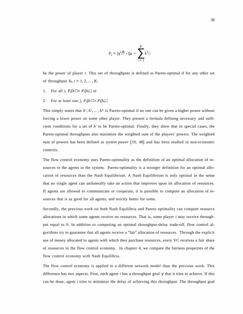
38

Pi = (γi)βi • (µ − ∑K

i = 1

λi)

be the power of player i. This set of throughputs is defined as Pareto-optimal if for any other set

of throughput λi0, i = 1, 2, ... , K:

1. For all i, Pi(λi) = Pi(λi0), or

2. For at least one j, Pj(λj) > Pi(λi0).

This simply states that λ1, λ2, ... , λK is Pareto-optimal if no one can be given a higher power without

forcing a lower power on some other player. They present a formula defining necessary and suffi-

cient conditions for a set of λi to be Pareto-optimal. Finally, they show that in special cases, the

Pareto-optimal throughputs also maximize the weighted sum of the players′ powers. The weighted

sum of powers has been defined as system power [10, 48] and has been studied in non-economic

contexts.

The flow control economy uses Pareto-optimality as the definition of an optimal allocation of re-

sources to the agents in the system. Pareto-optimality is a stronger definition for an optimal allo-

cation of resources than the Nash Equilibrium. A Nash Equilibrium is only optimal in the sense

that no single agent can unilaterally take an action that improves upon its allocation of resources.

If agents are allowed to communicate or cooperate, it is possible to compute an allocation of re-

sources that is as good for all agents, and strictly better for some.

Secondly, the previous work on both Nash Equilibria and Pareto optimality can compute resource

allocations in which some agents receive no resources. That is, some player i may receive through-

put equal to 0. In addition to computing an optimal throughput-delay trade-off, flow control al-

gorithms try to guarantee that all agents receive a ″fair″ allocation of resources. Through the explicit

use of money allocated to agents with which they purchase resources, every VC receives a fair share

of resources in the flow control economy. In chapter 4, we compare the fairness properties of the

flow control economy with Nash Equilibria.

The flow control economy is applied to a different network model than the previous work. This

difference has two aspects. First, each agent i has a throughput goal γi that it tries to achieve. If this

can be done, agent i tries to minimize the delay of achieving this throughput. The throughput goal

39

is not a constraint, however, and the agent can settle for less throughput. In some sense, this is the

dual to the player payoff functions in the above games.

Another difference is that the flow control economy is based on a virtual circuit computer network.

In such a network, each agent has a predefined path connecting its source node to it single desti-

nation node. In practice, most networks are based on the virtual circuit model [9]. So, in this sense

the flow control economy is based on a more realistic network model.

2.2.4 Multiple Access Protocols

The problem of designing optimal multiple access protocols for broadcast communication networks

[81] has been studied using concepts and algorithms from economics. In this problem, there is a

broadcast communication medium being shared by multiple independent network nodes. The

ethernet [71] and packet radio networks [50] are examples of such networks. Each node or station

in the network has data packets generated by some source that it wishes to transmit over the net-

work. The communication medium is divided into fixed length slots. To transmit a packet, node

Ni waits until the next slot starts and then broadcasts the packet. If no other node Nj attempts to

transmit a packet during this slot, the packet transmitted by Ni is correctly received at its destina-

tion. If, however, Nj also attempts to transmit a packet during the slot used by Ni, a collision occurs

and neither packet is successfully transmitted.

Protocols for the multiple access problem assign a transmission probability pi to each node Ni. If

node Ni has a packet it wishes to transmit in the next available slot, it broadcasts this packet with

probability pi. If Ni does not send the packet during the slot, or there is a collision, another aspect

of the protocol determines the next slot to try. Figure 8 on page 40 depicts packets, slots and

collisions in a broadcast network. The problem examined in this section is computing the trans-

mission probabilities pi for each node Ni that optimizes throughput.

Many multiple access protocols have been proposed [56], and different protocols are optimal for

different traffic arrival patterns and assumptions. Yemini and Kleinrock [89, 90] showed that

previously known protocols that are optimal for differing assumptions are actually special cases of

Pareto-optimality.

Yemini and Kleinrock showed that optimal protocols achieve a balance between throughput and

silence. If node Ni has a packet to transmit at slot sj and does not, its throughput is diminished but

the throughput of other nodes benefits from the fact that they will not collide with Ni during slot

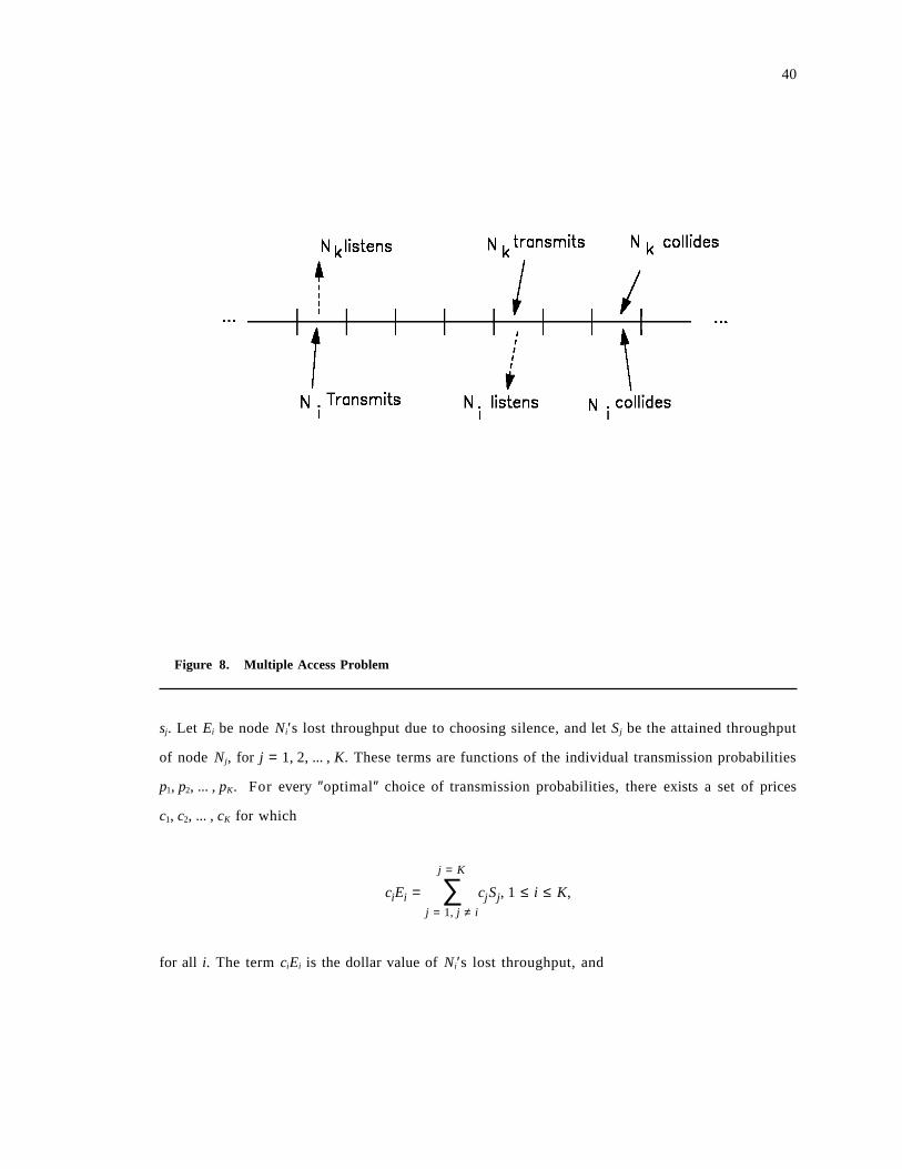
40

Figure 8. Multiple Access Problem

sj. Let Ei be node Ni′s lost throughput due to choosing silence, and let S j be the attained throughput

of node Nj, for j = 1, 2, ... , K. These terms are functions of the individual transmission probabilities

p1, p2, ... , pK. For every ″optimal″ choice of transmission probabilities, there exists a set of prices

c1, c2, ... , cK for which

ciEi = ∑j = K

j = 1, j ≠ i

cjSj, 1 ≤ i ≤ K,

for all i. The term ciEi is the dollar value of Ni′s lost throughput, and

41

∑j = K

j = 1, j ≠ i

cjSj

is the dollar value of the throughput attained by other nodes when Ni is silent. For a choice of

probabilities to be optimal, the dollar value of silence must equal the dollar value of total

throughput. Yemini and Kleinrock then show that various values of the cj correspond to previously

known optimal protocols.

Kurose, Yemini and Schwartz [55, 57] present a decentralized algorithm for computing the prices

that define the optimal transmission probabilities. Instead of attempting to optimize a common

system wide goal, each node attempts to maximize its individual throughput.

This algorithm is built on the concept of a fictitious resource. These resources capture the inter-

action between node Ni′s silence and Nj′s throughput. For each pair of nodes (i, j), there are two

fictitious communication resources xi → j and x j → i. These resources reflect the demanded trans-

mission probabilities of the node and the silence demanded of other nodes. For example,

1. x ii → j is Ni′s demand to Nj that Ni be allocated transmission probability x i

i → j.

2. Conversely, x ji → j is node Nj′s demand that Ni remain silent with probability x j

i → j.

The demands are similarly defined for x jj → i and x i

j → i. Since the fictitious resources are transmission

probabilities, x ii → j and x j

i → j are in the interval [0,1]. Furthermore, since x ii → j is Ni′s demand to

transmit with respect to its competitor Nj and x ji → j is competitor Nj′s demand that Ni remain silent,

these are only consistent if

x ii → j + x j

i → j = 1.

The economic model used for this algorithm is a pure Exchange Economy [40]. In this model, the

agents are not allocated money for purchasing resources. Instead, the supply of the resources is

assumed to be initially distributed among the agents in the economy. The agents then ″trade″ their

initial resource allocations for ones they consider better. The initial allocation of resources owned

by node Ni is called its endowment. In this economy, node Ni is allocated quantities of the two re-

sources that relate to its interaction with each other node Nj. These are x ii → j and x i

j → i. Node Ni′s

endowment of these resources is denoted

42

x ii → j, and x i

j → i.

For each fictitious resource x ii → j there is an associated price pi → j. These prices define the relative

value of the fictitious resources and determine the value of each node Ni′s endowment. The value

of the endowment is the revenue Ni could earn by selling its resources at the given prices. At any

set of prices

p• = {pi → j 1 ≤ i, j ≤ K and i ≠ j}

the wealth of node Ni is

Wi = ∑K

i = 1, i ≠ j

[pi → jxii → j + pj → ix

ij → i].

At a set of prices p•

, each node demands the allocation of fictitious resources that maximizes its

throughput subject to its budget constraints. The cost of the resources demanded by Ni at prices p•

cannot exceed the value of Ni′s initial allocation of resources at the current prices p•

. Formally, if

{x∼ i

i → j, x∼ i

j → i ∀(j ≠ i)} is Ni′s demand at p•

, then

∑K

i = 1, i ≠ j

[pi → jx∼ i

i → j + pj → ix∼ i

j → i] = ∑K

i = 1, i ≠ j

[pi → jxii → j + pj → ix

ij → i].

The algorithm for computing the optimal set of fictitious resources depends on the specific multiple

access protocol. Kurose, Yemini and Schwartz give algorithms for the Slotted Aloha Protocol

[2, 3] and for a time window protocol [55].

Since the resources represent probabilities, the demands are consistent only if

x ii → j + x j

i → j = 1

for all i, j. If,

x ii → j + x j

i → j > 1

43

resource xi → j is under priced, and pi → j should be increased. If, however,

x ii → j + x j

i → j < 1

the price pi → j is too low and should be increased. In their algorithm, Kurose, Schwartz and Yemini

use a tatonement process to update prices. The update is defined by the following formula:

pi → j = pi → j + ci → j[1 − x ii → j − x j

i → j],

where ci → j is a step size constant.

Kurose, Yemini and Schwartz proved that if their economy computed an equilibrium in which

x ii → j + x j

i → j = 1

for all i, j, then the allocation was Pareto-optimal. Proving that an equilibrium price vector exists,

and that this algorithm converges are extremely difficult problems. Kurose, Yemini and Schwartz

show that the demand of the nodes in this network are not continuous, and standard techniques

from economics cannot be applied to prove existence of equilibrium.

Kurose, Yemini and Schwartz implemented and simulated their economy for a 4 node network.

These simulations demonstrated empirically that the tatonement process converged to an equilib-

rium. They also showed that their economy rediscovered previously known optimal transmission

probabilities for the Slotted Aloha Protocol. Finally, they examined the effectiveness of the initial

endowment of resources to agents as a priority mechanism. The simulations revealed that increasing

the initial endowment did increase the equilibrium throughput of an agent.

The main disadvantage of this work is complexity. For a K node system, there is one physical re-

source (communication medium) but there are K2 − K fictitious resources that the economy must

allocate.

44

3.0 The Load Balancing Economy

This chapter presents an economy that uses decentralized competition and a price system to per-

form load balancing. The load balancing problem in a distributed system is to allocate CPU and

communication resources to jobs entering the system to minimize the average response time [29].

The load balancing economy is implemented and tested on the Network Simulation Testbed

(NEST) [25]. As with previous dynamic load balancing algorithms, the load balancing economy

cannot be evaluated analytically [29]. A simulation study is presented to evaluate the economy′s

performance. The implementation and simulation study also allow us to evaluate the software

structure of the economy, and determine its complexity.

The main result of this section is a set of experiments that shows that the economy substantially

improves performance for a wide choice of system configurations and agent behavior rules. We

compare the economy to a representative, non-economic load balancing algorithm, and exper-

iments demonstrate that the economy achieves better performance. Experiments also show that the

economy implements a broad spectrum of load balancing strategies and can adapt its strategy to the

relative power of CPU vs. communication. Finally, experiments evaluate the effects of the price

system on individual jobs. These are: 1) Flow control of poor jobs, 2) Job wealth as a priority

mechanism.

Section 1 defines the load balancing problem and the model of the underlying distributed system.

Section 2 describes the load balancing economy and presents a running example. The main results

of this chapter are contained in section 3. This section presents the results of several experiments

that measure the performance of the economy and compare it to a non-economic load balancing

algorithm. Section 4 is a comparative survey of previous work on load balancing. Section 5 contains

a conclusion and discusses directions for future work. There are two appendices to this chapter.

The first is a discussion of some the issues raised in this chapter. The second is a detailed de-

scription of the non-economic load balancing algorithm used for the comparisons in section 3.

3.1 Problem Statement and System Model

The distributed system consists of N processing nodes P1, ... , PN. The CPU power of node Pi is

defined by a processing speed parameter ri. A job that requires µ CPU seconds on an idealized

processor with r = 1, requires µri

seconds on processor Pi. The processors are connected by a

45

point-to-point network defined by an edge set E = {ei,j}. Edge ei,j represents a unidirectional com-

munication link connecting processors Pi and Pj. This link has a delay of d• seconds per byte.

Jobs originate at all processing nodes and seek CPU time on any processor. A job must leave the

system at its original node. The service requirements of a job are defined by

1. µ - The CPU service time of the job on an idealized processor Pi with ri = 1.

2. ReqBC - The number of bytes needed to describe the job. Each time a job migrates from one

processor to another seeking CPU service, ReqBC bytes must be sent.

3. RspBC - The number of bytes needed to describe the result of executing the job.

The assumption that the resource demands of every job are known when it enters the system is not

realistic for all applications. There may be statistical information based on previous submissions

of the job, however. The system model of this chapter is an idealization of this case. Adding be-

havioral rules that allow agents to deal with incomplete knowledge is left for future work.

The load balancing problem is to design an algorithm that minimizes mean job waiting time by

migrating jobs to balance the workloads of the processor nodes. The algorithm should be effective

over a broad range of distributed system configurations.

3.2 The Economy

The load balancing economy regulates the sharing of CPU time and communication capacity.

Each job J is provided with an initial allocation of money mJ with which it tries to purchase µJ

ri

CPU seconds on some processor Pi. The policy for assigning the initial endowment is discussed

later. The job is allowed to migrate through the system in search of CPU service, but it must pay

each time it crosses a link.

Processor nodes sell CPU time and communication bandwidth to the jobs. Processor node Pi in-

dependently sets the prices it charges for its local CPU and each link ei,j. Pi′s goal is to maximize

revenue. Each processor node Pi advertises its resource prices in bulletin boards at Pi and adjacent

nodes.

3.2.1 The Jobs

A job performs three operations to purchase resources. These are: (1) Compute a Budget Set, (2)

Apply a Preference Relation to the elements of the budget set and (3) Generate a Bid for the most

preferred budget set element.

46

We will use a running example to illustrate job behavior. Figure 9 on page 47 depicts a small dis-

tributed system. There are two jobs at processor P1. J1 has µ = 30 ms and J2 has µ = 10 ms. Both

jobs have been allocated $25 to purchase their resources and both have

ReqBC = RspBC = 1000 bytes. The dollar figures next to each node and data link represent the in-

formation in P1′s Bulletin Board. CPU time at P1 is selling for $1.00 per millisecond. The last ad-

vertised CPU prices at P2 and P3 are $0.10 per ms and $0.75 per ms respectively. The current price

P1 is charging to get to P2 is $0.001 per byte and the cost to get to P3 is $0.002 per byte. How P1

sets these prices is described below. In this figure, all processors have a CPU rate of 1 and each data

link has capacity 1 Mb/second.

3.2.1.1 Compute the Budget Set

Let mJ be job J′s wealth. A budget set element is an ordered pair (k, Ck) with Ck ≤ mJ. Ck is the

estimated cost of servicing job J at Pk. Ck is composed of:

1. The cost of buying µJ

rk CPU seconds at Pk.

2. The cost to cross the link to get to Pk.

3. The cost to get from Pk to the processor at which J entered the system.

The local bulletin board contains the price information used to compute Ck. Prices for local re-

sources are exact, but the prices for remote resources are only estimates. These prices may change

as J migrates through the network.

In our example, the budget sets for J1 and J2 are:

• B1 = {(2,$5.00)}.

• B2 = {(1,$10),(2,$3),(3,$11.50)}.

3.2.1.2 Computing Preferences

A job J must decide which element of its budget set is ″best.″ To do so, the job uses a Preference

Relation that imposes a partial ordering on the elements of the budget set. This relation is denoted

• J, and (j, Cj) • J (k, Ck), if J prefers service at Pj at cost Cj at least as much as service at Pk at cost

Ck. We consider three preference relations:

1. Price - The job wants to be serviced as cheaply as possible. In our example, both J1 and J2

prefer service at P2.

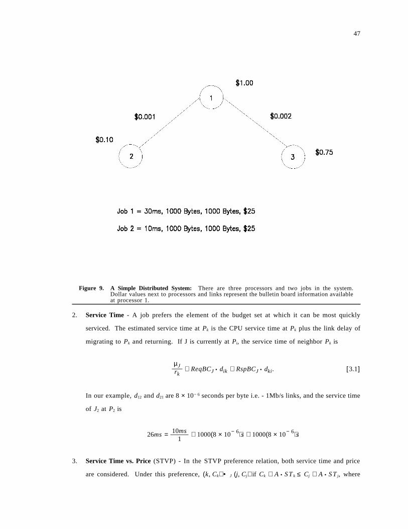
47

Figure 9. A Simple Distributed System: There are three processors and two jobs in the system.Dollar values next to processors and links represent the bulletin board information availableat processor 1.

2. Service Time - A job prefers the element of the budget set at which it can be most quickly

serviced. The estimated service time at Pk is the CPU service time at Pk plus the link delay of

migrating to Pk and returning. If J is currently at Pi, the service time of neighbor Pk is

µJrk

+ ReqBCJ • dik + RspBCJ • dki. [3.1]

In our example, d12 and d21 are 8 × 10− 6 seconds per byte i.e. - 1Mb/s links, and the service time

of J2 at P2 is

26ms = 10ms1

+ 1000(8 × 10− 6)s + 1000(8 × 10− 6)s

3. Service Time vs. Price (STVP) - In the STVP preference relation, both service time and price

are considered. Under this preference, (k, Ck) • J (j, Cj) if Ck + A • S T k ≤ Cj + A • S T j, where

48

1) S T k is the service time at Pk given by formula [3.1], and 2) A is a constant that defines the

relative importance of service time versus cost. In our example if A = 1, J2 prefers service at

P1, and if A = 0.1, J2 prefers service at P2.

3.2.1.3 Bid Generation

After computing the budget set and applying its preference relation, job J knows where it wants

to be serviced. The job now submits a bid for the next resource it needs. The next resource is either

the local CPU or a link to an adjacent node.

If J has mJ dollars remaining and the optimal element of the budget set is (k, Ck), then J′s estimated

surplus is mJ − Ck. In our example, J1′s estimated surplus at P2 is $20.

Job J bids the current price plus a fraction of its surplus defined by a parameter SJ. In our example,

the price for the link to P2 is $0.001, and J1′s surplus is $20. So, J1 will bid

$0.001 • ReqBC1 + ($25 − $5) • S1

for link e12. The effects of the parameter SJ are studied in the experiments discussed in section 3.3.5.

3.2.2 Processors

A processor node Pi performs three functions:

1. Auction Resources : When a resource (link or CPU) becomes idle, Pi holds an auction to de-

termine which of the jobs gets the resource next.

2. Advertise : Based on a local price change, Pi may send an advertisement message to its neigh-

bors.

3. Update Prices : Using arriving advertisements and the results of local auctions, Pi updates

prices in the local bulletin board.

3.2.2.1 Auction Resources

We studied two auction models for the economy. They are: 1) Sealed Bid and 2) A hybrid of Dutch

and English Auctions. Sealed Bid, Dutch and English Auctions auctions were described in chapter

2. The hybrid model tries to find the highest price that can be charged for a resource by increasing

the asking price when a bid is submitted (English), and decreasing the asking price when no bid is

submitted (Dutch). In both models, a job J is allowed to overbid using its surplus and SJ. This

allows strategy to play a role in the auction process. The effect of strategy is discussed later.

49

3.2.2.2 Price Updates

When a processor sells a resource to a job, the resource ′s entry in the bulletin board is set to the

unit price of the sale. In our example, if S2 = 0.33 and the Service Time preference is used, J2 will

bid

$15.00 = $1.00 • µ2 + 0.33 • ($25 − $10)

for P1′s CPU, and if S1 = 0.25, J1 will bid

$6.00 = $0.001 • ReqBC + 0.25 • ($25 − $5)

for link e12. If these are the winning bids, P1 sets its CPU price to $1.50 = $15/10 and the price for

link e12 to $0.006 = $6.00/1000.

3.2.2.3 Advertising

Each time the CPU price changes at a processor, the processor broadcasts the new price to all of

its neighbors. In our example, P2 and P3 are told of P1′s new CPU price of $1.50 per millisecond.

They insert this new value in their bulletin boards so that jobs at these processors can make deci-

sions regarding service at P1. The overhead of the advertisement policy and alternate policies are

discussed in the appendix.

3.3 Performance Experiments

We implemented the behavioral rules for the processors and jobs on Columbia University ′s Net-

work Simulation Testbed (NEST) [25]. We then simulated the system to measure the performance

and behavior of the economy. The distributed system we simulated was a nine processor mesh

(Figure 10 on page 51). The processing rate of each processor was 1.0, i.e. - a homogeneous system,

and each communication link had a capacity of 1 Mb/s.

In the simulation, jobs arrive at all processors in the system. The jobs′ service times were drawn

from an exponential distribution with a mean service time of 30 ms. The arrival process was as-

sumed to be Poisson with the same rate at all processors. The mean inter-arrival time was varied

to generate system utilizations from 0 to 90 percent. We also assumed that both the ReqBC and

RspBC parameters were the same for all jobs and fixed at 1000 bytes. Except for the experiments

of section 3.3.5, all jobs were allocated $5.

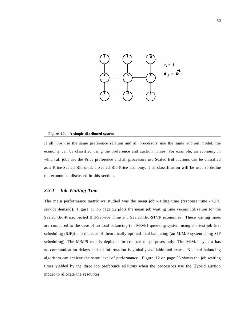
50

Figure 10. A simple distributed system

If all jobs use the same preference relation and all processors use the same auction model, the

economy can be classified using the preference and auction names. For example, an economy in

which all jobs use the Price preference and all processors use Sealed Bid auctions can be classified

as a Price-Sealed Bid or as a Sealed Bid-Price economy. This classification will be used to define

the economies discussed in this section.

3.3.1 Job Waiting Time

The main performance metric we studied was the mean job waiting time (response time - CPU

service demand). Figure 11 on page 52 plots the mean job waiting time versus utilization for the

Sealed Bid-Price, Sealed Bid-Service Time and Sealed Bid-STVP economies. These waiting times

are compared to the case of no load balancing (an M/M/1 queueing system using shortest-job-first

scheduling (SJF)) and the case of theoretically optimal load balancing (an M/M/9 system using SJF

scheduling). The M/M/9 case is depicted for comparison purposes only. The M/M/9 system has

no communication delays and all information is globally available and exact. No load balancing

algorithm can achieve the same level of performance. Figure 12 on page 53 shows the job waiting

times yielded by the three job preference relations when the processors use the Hybrid auction

model to allocate the resources.

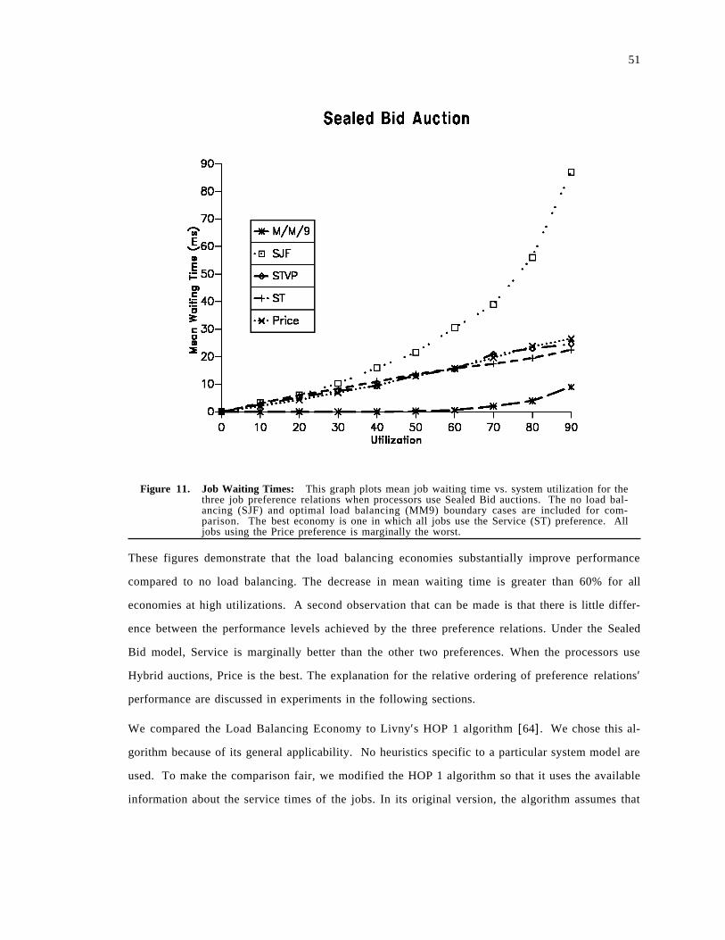
51

Figure 11. Job Waiting Times: This graph plots mean job waiting time vs. system utilization for thethree job preference relations when processors use Sealed Bid auctions. The no load bal-ancing (SJF) and optimal load balancing (MM9) boundary cases are included for com-parison. The best economy is one in which all jobs use the Service (ST) preference. Alljobs using the Price preference is marginally the worst.

These figures demonstrate that the load balancing economies substantially improve performance

compared to no load balancing. The decrease in mean waiting time is greater than 60% for all

economies at high utilizations. A second observation that can be made is that there is little differ-

ence between the performance levels achieved by the three preference relations. Under the Sealed

Bid model, Service is marginally better than the other two preferences. When the processors use

Hybrid auctions, Price is the best. The explanation for the relative ordering of preference relations′

performance are discussed in experiments in the following sections.

We compared the Load Balancing Economy to Livny′s HOP 1 algorithm [64]. We chose this al-

gorithm because of its general applicability. No heuristics specific to a particular system model are

used. To make the comparison fair, we modified the HOP 1 algorithm so that it uses the available

information about the service times of the jobs. In its original version, the algorithm assumes that

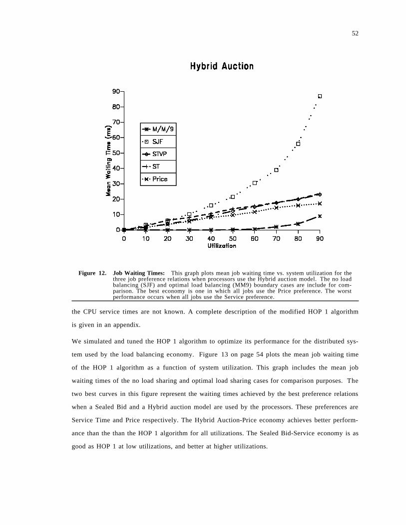
52

Figure 12. Job Waiting Times: This graph plots mean job waiting time vs. system utilization for thethree job preference relations when processors use the Hybrid auction model. The no loadbalancing (SJF) and optimal load balancing (MM9) boundary cases are include for com-parison. The best economy is one in which all jobs use the Price preference. The worstperformance occurs when all jobs use the Service preference.

the CPU service times are not known. A complete description of the modified HOP 1 algorithm

is given in an appendix.

We simulated and tuned the HOP 1 algorithm to optimize its performance for the distributed sys-

tem used by the load balancing economy. Figure 13 on page 54 plots the mean job waiting time

of the HOP 1 algorithm as a function of system utilization. This graph includes the mean job

waiting times of the no load sharing and optimal load sharing cases for comparison purposes. The

two best curves in this figure represent the waiting times achieved by the best preference relations

when a Sealed Bid and a Hybrid auction model are used by the processors. These preferences are

Service Time and Price respectively. The Hybrid Auction-Price economy achieves better perform-

ance than the than the HOP 1 algorithm for all utilizations. The Sealed Bid-Service economy is as

good as HOP 1 at low utilizations, and better at higher utilizations.

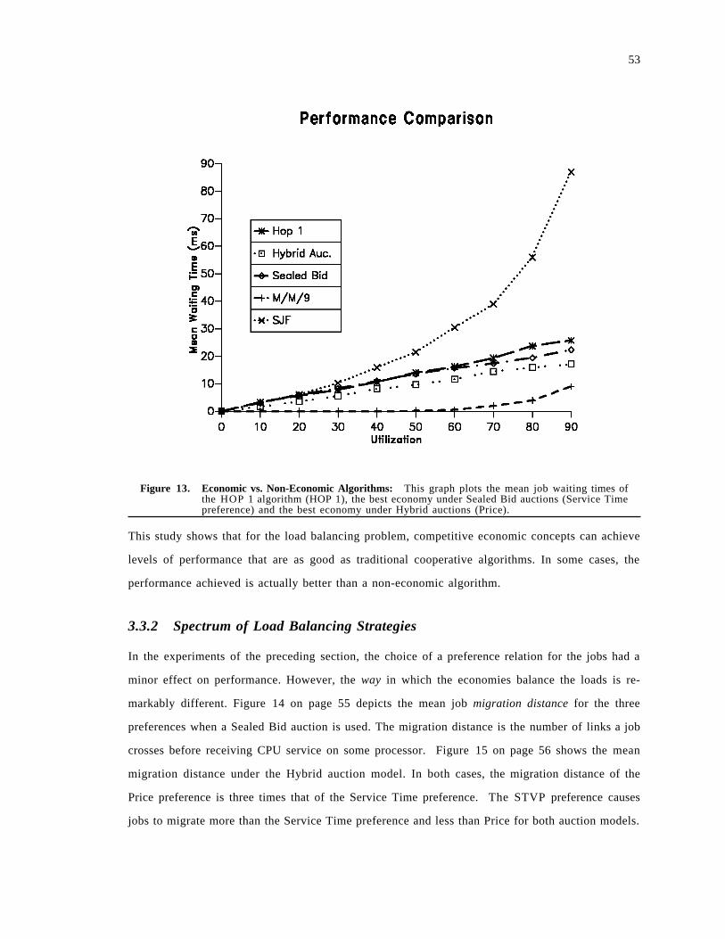
53

Figure 13. Economic vs. Non-Economic Algorithms: This graph plots the mean job waiting times ofthe HOP 1 algorithm (HOP 1), the best economy under Sealed Bid auctions (Service Timepreference) and the best economy under Hybrid auctions (Price).

This study shows that for the load balancing problem, competitive economic concepts can achieve

levels of performance that are as good as traditional cooperative algorithms. In some cases, the

performance achieved is actually better than a non-economic algorithm.

3.3.2 Spectrum of Load Balancing Strategies

In the experiments of the preceding section, the choice of a preference relation for the jobs had a

minor effect on performance. However, the way in which the economies balance the loads is re-

markably different. Figure 14 on page 55 depicts the mean job migration distance for the three

preferences when a Sealed Bid auction is used. The migration distance is the number of links a job

crosses before receiving CPU service on some processor. Figure 15 on page 56 shows the mean

migration distance under the Hybrid auction model. In both cases, the migration distance of the

Price preference is three times that of the Service Time preference. The STVP preference causes

jobs to migrate more than the Service Time preference and less than Price for both auction models.

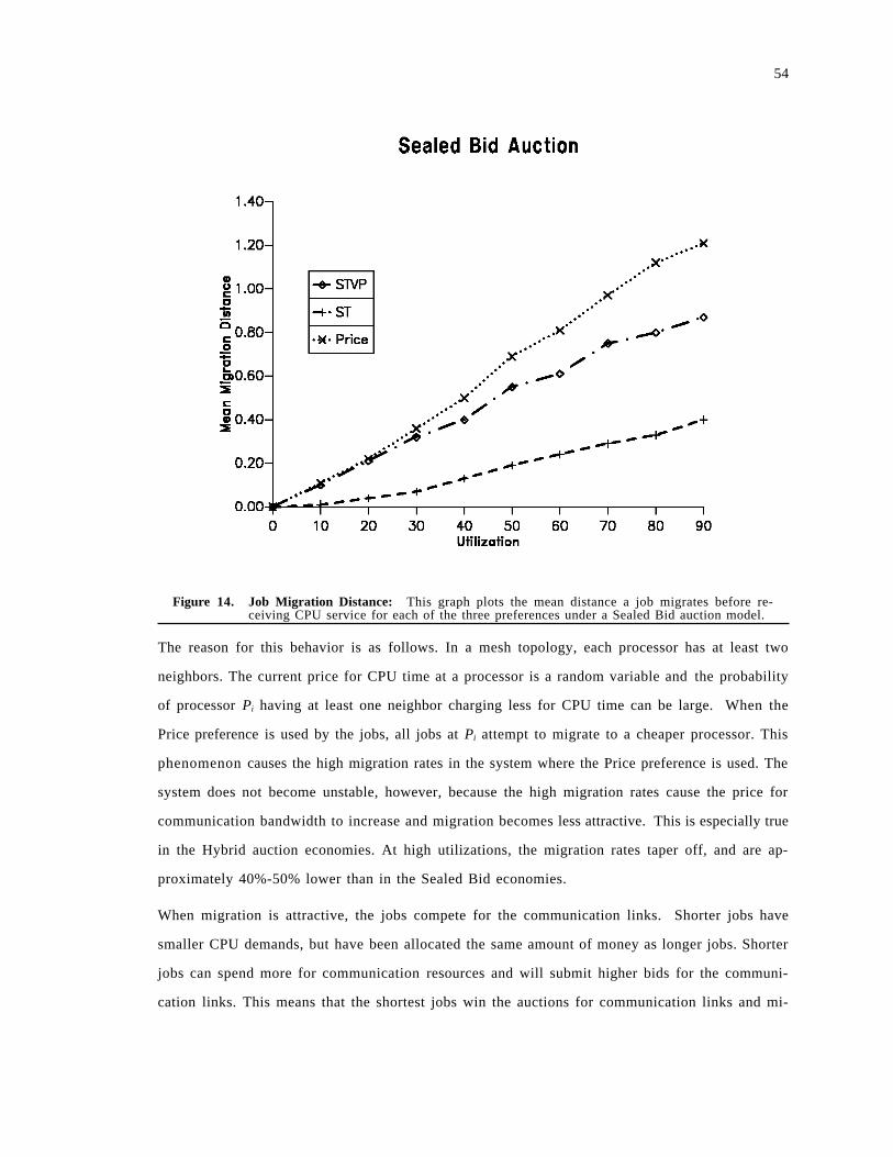
54

Figure 14. Job Migration Distance: This graph plots the mean distance a job migrates before re-ceiving CPU service for each of the three preferences under a Sealed Bid auction model.

The reason for this behavior is as follows. In a mesh topology, each processor has at least two

neighbors. The current price for CPU time at a processor is a random variable and the probability

of processor Pi having at least one neighbor charging less for CPU time can be large. When the

Price preference is used by the jobs, all jobs at Pi attempt to migrate to a cheaper processor. This

phenomenon causes the high migration rates in the system where the Price preference is used. The

system does not become unstable, however, because the high migration rates cause the price for

communication bandwidth to increase and migration becomes less attractive. This is especially true

in the Hybrid auction economies. At high utilizations, the migration rates taper off, and are ap-

proximately 40%-50% lower than in the Sealed Bid economies.

When migration is attractive, the jobs compete for the communication links. Shorter jobs have

smaller CPU demands, but have been allocated the same amount of money as longer jobs. Shorter

jobs can spend more for communication resources and will submit higher bids for the communi-

cation links. This means that the shortest jobs win the auctions for communication links and mi-

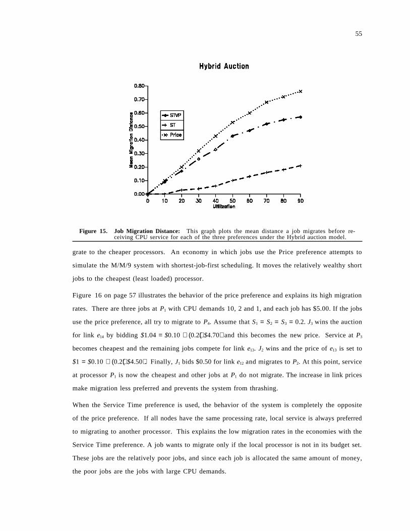
55

Figure 15. Job Migration Distance: This graph plots the mean distance a job migrates before re-ceiving CPU service for each of the three preferences under the Hybrid auction model.

grate to the cheaper processors. An economy in which jobs use the Price preference attempts to

simulate the M/M/9 system with shortest-job-first scheduling. It moves the relatively wealthy short

jobs to the cheapest (least loaded) processor.

Figure 16 on page 57 illustrates the behavior of the price preference and explains its high migration

rates. There are three jobs at P1 with CPU demands 10, 2 and 1, and each job has $5.00. If the jobs

use the price preference, all try to migrate to P4. Assume that S1 = S2 = S3 = 0.2. J3 wins the auction

for link e14 by bidding $1.04 = $0.10 + (0.2)($4.70) and this becomes the new price. Service at P3

becomes cheapest and the remaining jobs compete for link e13. J2 wins and the price of e13 is set to

$1 = $0.10 + (0.2)($4.50). Finally, J1 bids $0.50 for link e12 and migrates to P2. At this point, service

at processor P1 is now the cheapest and other jobs at P1 do not migrate. The increase in link prices

make migration less preferred and prevents the system from thrashing.

When the Service Time preference is used, the behavior of the system is completely the opposite

of the price preference. If all nodes have the same processing rate, local service is always preferred

to migrating to another processor. This explains the low migration rates in the economies with the

Service Time preference. A job wants to migrate only if the local processor is not in its budget set.

These jobs are the relatively poor jobs, and since each job is allocated the same amount of money,

the poor jobs are the jobs with large CPU demands.

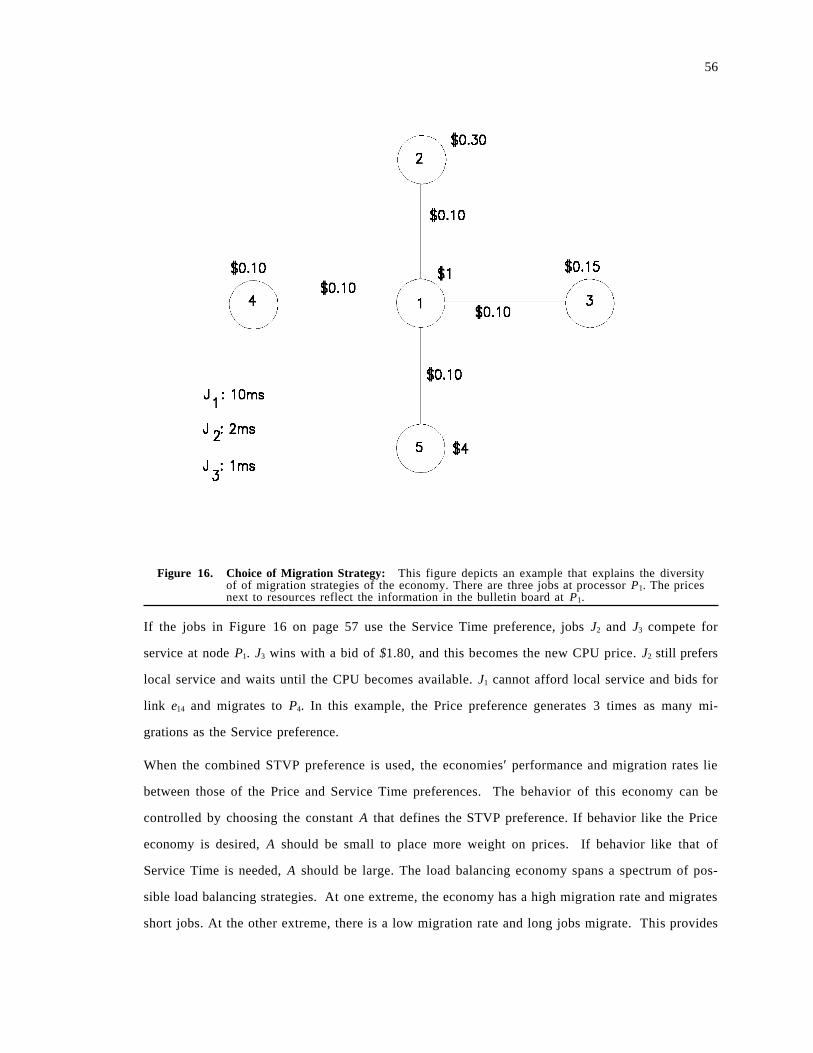
56

Figure 16. Choice of Migration Strategy: This figure depicts an example that explains the diversityof of migration strategies of the economy. There are three jobs at processor P1. The pricesnext to resources reflect the information in the bulletin board at P1.

If the jobs in Figure 16 on page 57 use the Service Time preference, jobs J2 and J3 compete for

service at node P1. J3 wins with a bid of $1.80, and this becomes the new CPU price. J2 still prefers

local service and waits until the CPU becomes available. J1 cannot afford local service and bids for

link e14 and migrates to P4. In this example, the Price preference generates 3 times as many mi-

grations as the Service preference.

When the combined STVP preference is used, the economies′ performance and migration rates lie

between those of the Price and Service Time preferences. The behavior of this economy can be

controlled by choosing the constant A that defines the STVP preference. If behavior like the Price

economy is desired, A should be small to place more weight on prices. If behavior like that of

Service Time is needed, A should be large. The load balancing economy spans a spectrum of pos-

sible load balancing strategies. At one extreme, the economy has a high migration rate and migrates

short jobs. At the other extreme, there is a low migration rate and long jobs migrate. This provides

57

flexibility that allows the implementer of the load balancing algorithm to choose a particular point

in the spectrum by setting a single parameter.

3.3.3 Adapting to CPU vs. Communication

Figure 17 on page 58 plots the performance of the Load Balancing Economy and the HOP 1 al-

gorithm when the speeds of the communication links have been cut in half (i.e. - 512Kb/s). The

three economies use Sealed Bid auctions and the Price, Service Time and STVP preferences. In this

system, the Service Time preference yields substantially better performance than either of the other

preferences, and is better than the HOP 1 algorithm at high utilizations. The Service Time prefer-

ence is now 25% better than the other two preferences at high utilization as opposed to 15% in the

case in which the link speeds were 1Mb/s.

Figure 18 on page 59 shows the situation when the communication speeds have doubled to 2 Mb/s.

Service Time and HOP1 are now the worst, and Price and the STVP preferences are approximately

10% better. This is in contrast to the fact that Price is the worst preference in the systems with

1Mb/s and 512Kb/s links.

The reasons for the changes in relative performance are due to the migration rates of jobs using the

preferences. When the Price preference is used, the economy is very aggressive and has a very high

migration rate. There is no disincentive under the Price preference for a very high migration rate

when the speed of the communication links has been halved. The Price preference does not take

the link and CPU speeds into consideration when ranking budget set elements. In the example of

Figure 16, the sequence of job decisions under the Price preferences does not change if link speeds

are decreased. The high migration rate continues to occur despite the decrease in communication

speed. This strategy becomes progressively worse as link speeds decrease.

The Service Time preference generates a very low migration rate independently of the relative speed

of communication to CPU power. As long as the communication speed is finite and the CPUs have

the same processing rates, local service is always strictly preferred. The example of Service Time

behavior in Figure 16 is independent of link speeds. The Service Time preference does well when

the communication speed has been halved since it has a low migration rate and migrates the long

jobs.

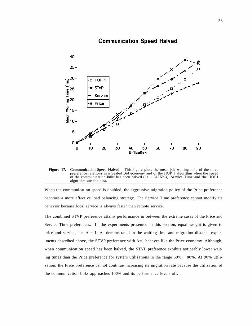
58

Figure 17. Communication Speed Halved: This figure plots the mean job waiting time of the threepreference relations in a Sealed Bid economy and of the HOP 1 algorithm when the speedof the communication links has been halved (i.e. - 512Kb/s). Service Time and the HOP1algorithm are the best.

When the communication speed is doubled, the aggressive migration policy of the Price preference

becomes a more effective load balancing strategy. The Service Time preference cannot modify its

behavior because local service is always faster than remote service.

The combined STVP preference attains performance in between the extreme cases of the Price and

Service Time preferences. In the experiments presented in this section, equal weight is given to

price and service, i.e. A = 1. As demonstrated in the waiting time and migration distance exper-

iments described above, the STVP preference with A=1 behaves like the Price economy. Although,

when communication speed has been halved, the STVP preference exhibits noticeably lower wait-

ing times than the Price preference for system utilizations in the range 60% − 80%. At 90% utili-

zation, the Price preference cannot continue increasing its migration rate because the utilization of

the communication links approaches 100% and its performance levels off.

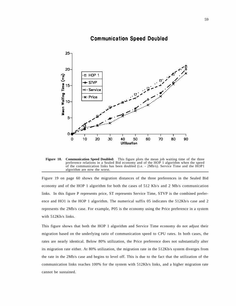
59

Figure 18. Communication Speed Doubled: This figure plots the mean job waiting time of the threepreference relations in a Sealed Bid economy and of the HOP 1 algorithm when the speedof the communication links has been doubled (i.e. - 2Mb/s). Service Time and the HOP1algorithm are now the worst.

Figure 19 on page 60 shows the migration distances of the three preferences in the Sealed Bid

economy and of the HOP 1 algorithm for both the cases of 512 Kb/s and 2 Mb/s communication

links. In this figure P represents price, ST represents Service Time, STVP is the combined prefer-

ence and HO1 is the HOP 1 algorithm. The numerical suffix 05 indicates the 512Kb/s case and 2

represents the 2Mb/s case. For example, P05 is the economy using the Price preference in a system

with 512Kb/s links.

This figure shows that both the HOP 1 algorithm and Service Time economy do not adjust their

migration based on the underlying ratio of communication speed to CPU rates. In both cases, the

rates are nearly identical. Below 80% utilization, the Price preference does not substantially alter

its migration rate either. At 80% utilization, the migration rate in the 512Kb/s system diverges from

the rate in the 2Mb/s case and begins to level off. This is due to the fact that the utilization of the

communication links reaches 100% for the system with 512Kb/s links, and a higher migration rate

cannot be sustained.

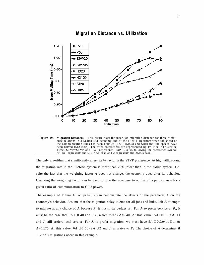
60

Figure 19. Migration Distances: This figure plots the mean job migration distance for three prefer-ence relations in a Sealed Bid Economy and of the HOP 1 algorithm when the speed ofthe communication links has been doubled (i.e. - 2Mb/s) and when the link speeds havebeen halved (512 Kb/s). The three preferences are represented by P=Price, ST=ServiceTime, STVP=STVP and HO1 represents HOP 1. A 05 following the preference symbolor HO1 represents the 512 Kb/s case and 2 represents the 2Mb/s case.

The only algorithm that significantly alters its behavior is the STVP preference. At high utilizations,

the migration rate in the 512Kb/s system is more than 20% lower than in the 2Mb/s system. De-

spite the fact that the weighting factor A does not change, the economy does alter its behavior.

Changing the weighting factor can be used to tune the economy to optimize its performance for a

given ratio of communication to CPU power.

The example of Figure 16 on page 57 can demonstrate the effects of the parameter A on the

economy′s behavior. Assume that the migration delay is 2ms for all jobs and links. Job J3 attempts

to migrate at any choice of A because P1 is not in its budget set. For J2 to prefer service at P4, it

must be the case that 6A + 0.40<2 A + 2, which means A<0.40. At this value, 5A + 0.30> A + 1

and J3 still prefers local service. For J3 to prefer migration, we must have 5A + 0.30< A + 1, or

A<0.175. At this value, 6A + 0.50<2 A + 2 and J2 migrates to P3. The choice of A determines if

1, 2 or 3 migrations occur in this example.

61

In summary, the Load Balancing Economy is very versatile and offers a spectrum of load balancing

strategies. Different strategies are better for differing ratios of communication to CPU speeds. It is

possible to tune the economy to this ratio by adjusting a single weighting factor, and this can offer

substantial performance improvements over a non-economic load balancing algorithm. The main

disadvantage to this approach is that manual intervention is required to adjust the weighting factor.

3.3.4 Flow Control

The Load Balancing Economy implements flow control at high utilizations. Figure 20 on page 62

plots the job throughput as a function of system utilization. This figure shows the three preference

relations in a Hybrid auction economy, and the HOP 1 algorithm. Above 60% utilization, the

economies′ throughputs taper off. This is caused by the intense competition at high utilizations.

Relatively poor jobs or jobs that make poor resource purchasing decisions enter a situation in

which they cannot acquire the resources needed to complete processing and leave the system. This

improves the performance of the wealthier jobs by decreasing the effective utilization of the system.

Throughput is decreased to improve response time.

The form of flow control implemented has some drawbacks. First, the flow control does not pre-

vent jobs from entering the system. Instead, the jobs enter the system and are denied resources. A

user that submits a job does not know if the job will be serviced or not because there is no way to

tell if the job will eventually receive service. Secondly, the jobs that are flow controlled remain in

the system but cannot purchase any resources. The amount of storage used to hold idle jobs in-

creases monotonically over time. Obviously, this cannot be allowed to occur indefinitely. Potential

solutions to these problems are discussed in an appendix. The main problem with the flow control

mechanism implemented by the load balancing economy is that it cannot easily be controlled.

Unlike adapting to the CPU/Communication speed ratio, there is no effective way to set the desired

throughput/response time goal. Correcting these deficiencies is an area for future work.

3.3.5 Wealth, Priority and Learning

A Job J′s bidding rule has two parameters. The first is SJ, which determines J′s use of surplus funds.

The second parameters is a feedback factor δJ. Each time J wins an auction, it sets SJ = SJ − δJ.

When J loses, it updates S j = SJ + δJ. The use of the feedback δJ implements a simple learning

mechanism. The goal is to learn the minimum use of surplus funds needed to win an auction.

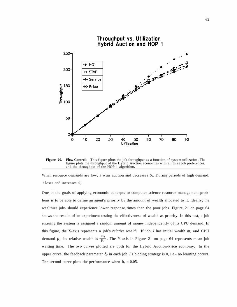
62

Figure 20. Flow Control: This figure plots the job throughput as a function of system utilization. Thefigure plots the throughput of the Hybrid Auction economies with all three job preferences,and the throughput of the HOP 1 algorithm.

When resource demands are low, J wins auction and decreases SJ. During periods of high demand,

J loses and increases SJ.

One of the goals of applying economic concepts to computer science resource management prob-

lems is to be able to define an agent′s priority by the amount of wealth allocated to it. Ideally, the

wealthier jobs should experience lower response times than the poor jobs. Figure 21 on page 64

shows the results of an experiment testing the effectiveness of wealth as priority. In this test, a job

entering the system is assigned a random amount of money independently of its CPU demand. In

this figure, the X-axis represents a job′s relative wealth. If job J has initial wealth mJ and CPU

demand µJ, its relative wealth ismJ

µJ. The Y-axis in Figure 21 on page 64 represents mean job

waiting time. The two curves plotted are both for the Hybrid Auction-Price economy. In the

upper curve, the feedback parameter δJ in each job J′s bidding strategy is 0, i.e.- no learning occurs.

The second curve plots the performance when δJ = 0.05.

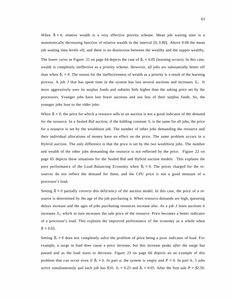
63

When δ = 0, relative wealth is a very effective priority scheme. Mean job waiting time is a

monotonically decreasing function of relative wealth in the interval [0, 0.80]. Above 0.08 the mean

job waiting time levels off, and there is no distinction between the wealthy and the supper wealthy.

The lower curve in Figure 21 on page 64 depicts the case of δJ = 0.05 (learning occurs). In this case,

wealth is completely ineffective as a priority scheme. However, all jobs are substantially better off

than when δJ = 0. The reason for the ineffectiveness of wealth as a priority is a result of the learning

process. A job J that has spent time in the system has lost several auctions and increases SJ. It

more aggressively uses its surplus funds and submits bids higher than the asking price set by the

processors. Younger jobs have lost fewer auctions and use less of their surplus funds. So, the

younger jobs lose to the older jobs.

When δ = 0, the price for which a resource sells in an auction is not a good indicator of the demand

for the resource. In a Sealed Bid auction, if the bidding constant SJ is the same for all jobs, the price

for a resource is set by the wealthiest job. The number of other jobs demanding the resource and

their individual allocations of money have no effect on the price. The same problem occurs in a

Hybrid auction. The only difference is that the price is set by the two wealthiest jobs. The number

and wealth of the other jobs demanding the resource is not reflected by the price. Figure 22 on

page 65 depicts these situations for the Sealed Bid and Hybrid auction models. This explains the

poor performance of the Load Balancing Economy when δJ = 0. The prices charged for the re-

sources do not reflect the demand for them, and the CPU price is not a good measure of a

processor′s load.

Setting δ > 0 partially corrects this deficiency of the auction model. In this case, the price of a re-

source is determined by the age of the job purchasing it. When resource demands are high, queueing

delays increase and the ages of jobs purchasing resources increase also. As a job J loses auctions it

increases SJ, which in turn increases the sale price of the resource. Price becomes a better indicator

of a processor′s load. This explains the improved performance of the economy as a whole when

δ = 0.05.

Setting δJ > 0 does not completely solve the problem of price being a poor indicator of load. For

example, a surge in load does cause a price increase, but this increase peaks after the surge has

passed and as the load starts to decrease. Figure 23 on page 66 depicts an an example of this

problem that can occur even if δJ > 0. In part a, the system is empty and P = 0. In part b, 3 jobs

arrive simultaneously and each job has $10, SJ = 0.25 and δJ = 0.05. After the first sale P = $2.50.

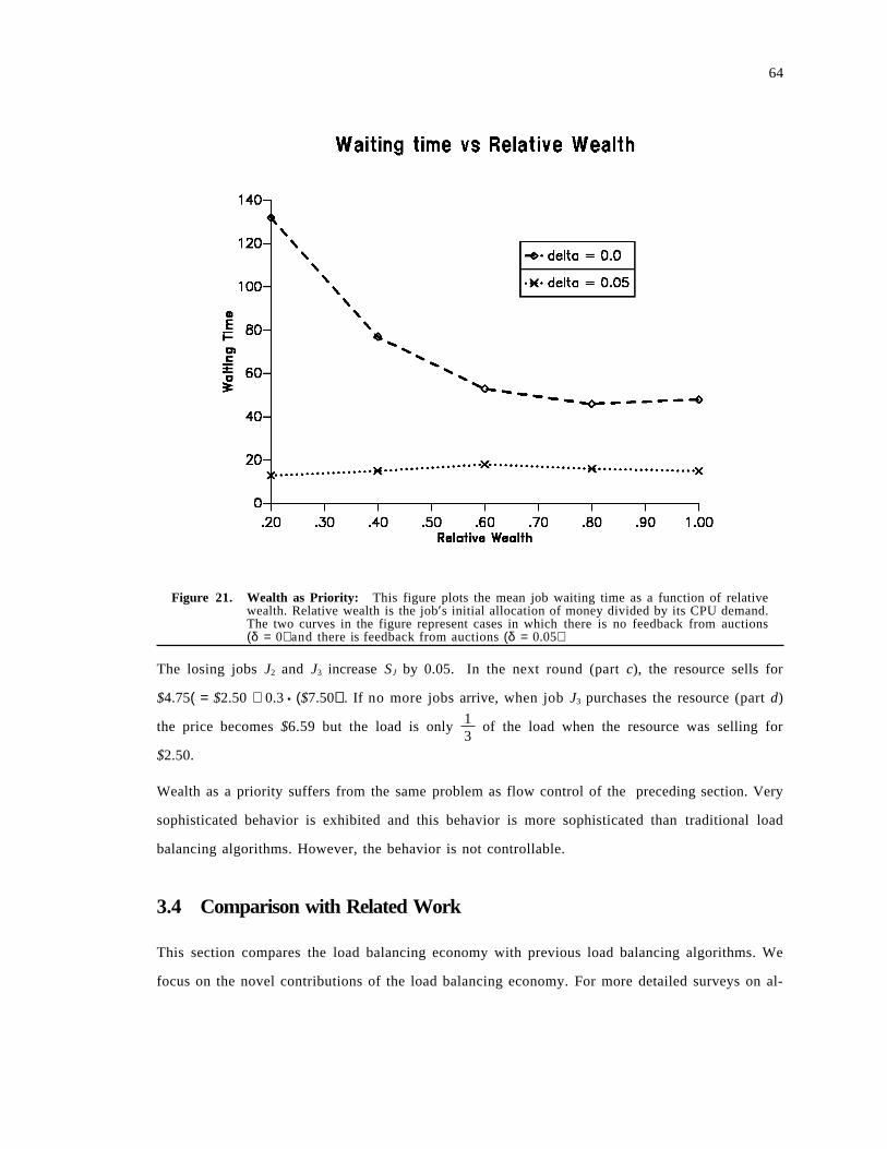
64

Figure 21. Wealth as Priority: This figure plots the mean job waiting time as a function of relativewealth. Relative wealth is the job′s initial allocation of money divided by its CPU demand.The two curves in the figure represent cases in which there is no feedback from auctions(δ = 0) and there is feedback from auctions (δ = 0.05)

The losing jobs J2 and J3 increase SJ by 0.05. In the next round (part c), the resource sells for

$4.75( = $2.50 + 0.3 • ($7.50)). If no more jobs arrive, when job J3 purchases the resource (part d)

the price becomes $6.59 but the load is only 13

of the load when the resource was selling for

$2.50.

Wealth as a priority suffers from the same problem as flow control of the preceding section. Very

sophisticated behavior is exhibited and this behavior is more sophisticated than traditional load

balancing algorithms. However, the behavior is not controllable.

3.4 Comparison with Related Work

This section compares the load balancing economy with previous load balancing algorithms. We

focus on the novel contributions of the load balancing economy. For more detailed surveys on al-

65

Figure 22. Auctions and Prices: This figure shows why auction prices do not accurately reflect de-mand. In this figure, 4 jobs bid for a resource R and all have S = 0.25. Values below jobsrepresent wealth and values next to arrows represent bids. In the Sealed Bid auction, thesale price is $2.50 whether or not J2, J3 and J4 demand the resource. In the Hybrid auction,J1 and J2 compete driving the price to $9.00, and J1 wins with a bid of $9.25. Jobs J3 and42 have no effect on the price.

gorithms, readers are referred to [29, 74]. Actual implementations of distributed systems that

support load balancing are discussed in [6, 46, 47].

The performance results presented in this chapter and previous work [26, 27, 44, 54, 64, 65]

demonstrate that the interprocessor communication medium has a major impact on the effective-

ness of load balancing. The communication medium has two sources of delay. The first is the static

delay of executing the communication protocols at the sender and receiver, and the transmission

delay on the link. These are the factors included in the definition of S T k in the job preference re-

lations. The second source of delay is queueing delay at these resources. Some previous work has

ignored the effects of the communication delay on performance [34, 35, 53, 74, 91]. Two con-

structive approaches to dealing with communication delays have studied. The first is to

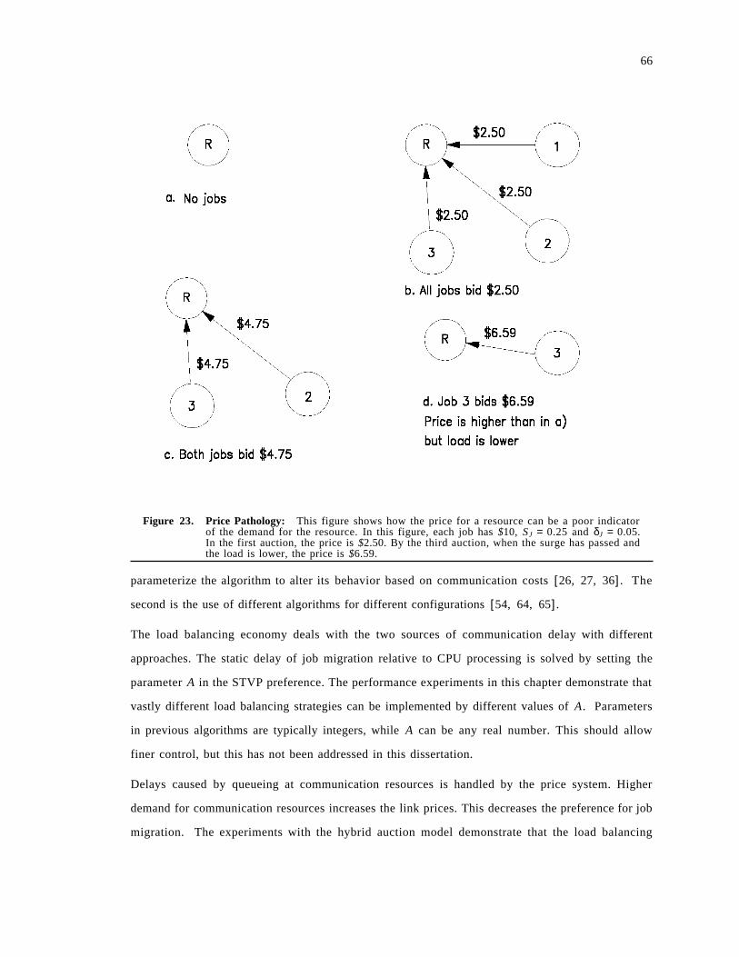
66

Figure 23. Price Pathology: This figure shows how the price for a resource can be a poor indicatorof the demand for the resource. In this figure, each job has $10, SJ = 0.25 and δJ = 0.05.In the first auction, the price is $2.50. By the third auction, when the surge has passed andthe load is lower, the price is $6.59.

parameterize the algorithm to alter its behavior based on communication costs [26, 27, 36]. The

second is the use of different algorithms for different configurations [54, 64, 65].

The load balancing economy deals with the two sources of communication delay with different

approaches. The static delay of job migration relative to CPU processing is solved by setting the

parameter A in the STVP preference. The performance experiments in this chapter demonstrate that

vastly different load balancing strategies can be implemented by different values of A. Parameters

in previous algorithms are typically integers, while A can be any real number. This should allow

finer control, but this has not been addressed in this dissertation.

Delays caused by queueing at communication resources is handled by the price system. Higher

demand for communication resources increases the link prices. This decreases the preference for job

migration. The experiments with the hybrid auction model demonstrate that the load balancing

67

economy decreases migration rates as the competition for communication resources increases. This

process does not require external control to set parameters. The load balancing economy is self-

regulating, and this behavior is not present in previous algorithms.

Stability has been identified as a problem for dynamic load balancing algorithms [12, 86]. An al-

gorithm is unstable if it can enter a state in which jobs are being migrated to balance loads but no

productive processing is being done. The phenomenon is similar to thrashing in virtual memory

[23]. Two approaches have been taken to ensure stable behavior. The first uses global information

to periodically compute assignments of work to processors to minimize a system wide performance

objective [34, 35]. The resulting assignment is fixed during the next interval and instability is

avoided. The overhead of acquiring consistent global information can make this approach un-

workable. The second solution to the stability problem is augmenting the load balancing algorithm

with a heuristic that prevents unstable states [26, 27, 36, 53, 54, 64, 65]. Two common

heuristics are:

1. Each job J can only be migrated M times by the algorithm. This prevents the system from

infinitely migrating jobs.

2. Let Li, Lj be the loads of processors Pi, Pj. A job can be transferred from Pi to Pj only if

Li − Lj > T , where T is a threshold parameter greater than the load of any single job. This

disallows migrations that would reverse the load imbalance, and prevents Pi and Pj from en-

tering a state in which they infinitely migrate jobs between each other.

There are two disadvantages to the use of heuristics. The first is increased complexity. The second

disadvantage is that the heuristics are pessimistic. The heuristics disallow migrations that may im-

prove performance to avoid the possibility of instability.

The load balancing economy is inherently stable. A job pays a non zero fee each time it crosses a

link. So, infinite migration is not possible. This mechanism implements a more general version of

heuristic 1 above. The link prices increase when there is competition. This has the desirable ad-

vantage that the distance a job is allowed to migrate decreases as the demand for communication

resources increases. The experiments with the hybrid auction model demonstrated that increased

competition for communication resources decreases the preferability of migration. This also pre-

vents instability. The sealed bid auction model is less effective in this respect.

Load balancing algorithms can be partitioned into to classes: sender initiated and receiver initiated

[27, 74]. In a sender initiated algorithm, over loaded processors look for under loaded processors

68

to which work can be sent. In a receiver initiated algorithm, under loaded processors search for over

loaded processors from which work can be obtained. It has been shown that at high average system

load receiver initiated algorithms achieve better performance, and at low average load sender initi-

ated are better [27, 74].

The load balancing economy is both sender and receiver initiated and can encompass the benefits

of both models. A heavily loaded processor charges a higher CPU price which causes jobs to look

for cheaper, less loaded processors. This implements sender initiated load balancing. The less loaded

processors advertise their lower CPU prices to attract migrating jobs (receiver initiated). The HOP

1 algorithm is sender initiated. A comparison between the load balancing economy and a receiver

initiated algorithm is an area of future work.

The load balancing economy limits complexity in several ways. First, all decision making is de-

centralized and this decentralization removes complexity due to cooperative protocols. The only

interaction between processors is inserting advertisements into bulletin boards. The processors do

not make decisions based on this information. All local auctions and price updates are performed

independently from other processors. The decision making rules of the jobs are independent.

The decentralized decision making allows a very modular implementation. It is possible to change

a processor′s auction model without effecting the policies of any other processor. In our exper-

iments, switching between sealed bid and the hybrid auction models did not require any changes

in the job′s rules. Similarly, varying a jobs preference relation does not require any modification to

other jobs or the processors. This modularity facilitates transparent addition of processor and job

rules and software maintenance.

Finally, the load balancing economy decreases complexity be eliminating the need for special

heuristics or alternate algorithms. Tuning the algorithm for the ratio of CPU vs Communication,

preventing instability and implementing sender/receiver initiated load balancing are inherent prop-

erties of the economy.

3.5 Summary

This chapter presented the load balancing economy. A simulation study showed that this economy

achieves substantially improved system performance compared to a distributed computer system in

which load balancing is not implemented. The economy was also compared with a non-economic

load balancing algorithm. It was shown that performance improvements achieved by all variations

69

of the load balancing economy are competitive with the improvements of the non-economic algo-

rithm, and in some cases the load balancing economy is strictly better.

The load balancing economy was shown to implement a very broad range of load balancing strat-

egies. The mean distance a job migrates in search of CPU service changes by a factor of 3 for dif-

ferent versions of the economy. The decision as to which type of job (short vs. long) should migrate

to balance loads also changes. This adaptability allows the economy to be optimized for the ratio

of communication to CPU power in the underlying distributed system.

The load balancing economy implements a form of flow control at high utilizations. Job through-

put is throttled to improve mean job response time. We studied the effectiveness of a the amount

of money allocated to a job as a definition of priority. The role of learning and its interactions with

the use of wealth as a priority scheme were addressed also.

We discussed how the load balancing economy limits complexity compared to previous load bal-

ancing algorithms by eliminating the need for multiple heuristics. Previous algorithms deal with

specific sub-problems of load balancing by applying ad hoc heuristics. These heuristics are not

necessary in the load balancing economy. The decentralized decision making in the load balancing

economy also limits complexity by implementing a set of modular, disjoint algorithms.

We discussed three shortcomings of the load balancing economy. The first is the potentially high

overhead of auctioning idle resources. The second is the inability of auctions to set resource prices

that accurately reflect the demand for the resources being sold. These two problems motivate our

use of different pricing mechanisms in the later chapters.

The third shortcoming is the assumption that a job′s CPU service demand is known when the job

is submitted. In general, economic models assume that individual agents know their resource de-

mands. This may not always be true for the load balancing problem, but there are environments

in which this assumption is realistic.

3.6 Appendix

3.6.1 Issues

The discussion of the design of the load balancing economy and of the performance experiments

pointed out disadvantages of the economy and raised other issues. These issues are addressed in this

appendix. The solutions to the disadvantages and issues raised are left for future work.

70

3.6.1.1 Knowledge of Resource Demands

The jobs′ behavioral rules rely heavily of the assumption that each job J knows its resource de-

mands (µJ, ReqBCJ, ReqBCJ). The assumption that individual agents know their resource demands

is an integral part of microeconomic models [40]. Modifying the algorithms to deal with incom-

plete information is left as an area of future research.

Modifying the economy to deal with incomplete information faces two problems which are

orthogonal to the economic algorithms. If no information about a job J′s CPU demand is known,

the information must be inferred from resource consumption as the job resides in the system. For

example, jobs can purchase time slices. The job′s total CPU demand can be estimated based on the

number of slices already purchased. This approach is similar to multilevel feedback queueing for

CPU scheduling in operating systems [23]. Bryant and Finkel [12] studied a load balancing model

in which job CPU demands were estimated based on service received. The main problem with this

approach is that load balancing must be preemptive, and migrate actively running jobs. It is typically

assumed that the communication and CPU overhead of preemptive load balancing is prohibitive

[75].

An alternate approach is to estimate the resource demands based on previous execution, or based

on job classes. This limits the generality of the system. Furthermore, computing these estimates

is time consuming and requires substantial resources itself [30].

3.6.1.2 Auctions

Section 3.5 pointed out several disadvantages of using auctions to allocate resources. An additional

problem is overhead. Each time a resource is allocated all locally residing jobs participate in an

auction to determine which job gets the resource. The overhead is a greater problem under the

hybrid model because there are multiple rounds of bidding. This overhead and the problems dis-

cussed in section 3.5 have led us to study alternate models in chapters 4 and 5. The data manage-

ment economy does successfully use an English Auction, however.

3.6.1.3 Advertisements

There is potentially an overhead problem associated with the processors′ advertisement policy.

Processing node Pi broadcasts every CPU price change to all neighbors. The advertisement mes-

sages are very small, and in a point-to-point network they can be piggybacked on normal data

transfer messages. The processing overhead for receiving an advertisement and updating the bulletin

71

board is also quite low. So, the advertisement policy′s overhead is tolerable in point-to-point net-

works.

Livny [64, 65] has shown that broadcasting all state changes can have a prohibitive effect on the

performance of distributed systems with a broadcast interconnect medium. In such an environment,

the load balancing economy requires heuristic rules to limit the amount of advertisements sent. For

example, only price changes greater than a threshold ∆ are sent. These heuristics add complexity,

however.

3.6.1.4 Price Guarantees

When job J decides to migrate from processor Pi to Pj it bases its decision on the CPU cost of Pj

contained in Pi′s bulletin board. This price is not guaranteed, and can change while J is migrating.

Furthermore, J participates in an auction for the CPU after it arrives at Pj and may not pay the

price advertised at Pi. These factors can generate fruitless migrations that consume communication

resources an incur overhead.

An alternate approach is to guarantee prices. In this case, if J sees price cj advertised in Pi′s bulletin

board, Pj must honor this commitment when J arrives. This policy greatly complicates the econ-

omy, however. Since prices are set by auctions, resource prices change rapidly. If n jobs arrive at

Pj, it is possible that each job has seen a different advertised price. Processor Pj must decide which

job to service next. Furthermore, it is not clear what price Pj should advertise when allocating the

CPU to one of these jobs. Finally, if a job was guaranteed a price cJj which is greater than the

current CPU price cj, should J be allowed to spend less? We avoided implementing guaranteed

pricing in the load balancing economy due to the complexity it incurs.

3.6.1.5 Flow Control

Section 3.4 pointed out two shortcomings of the flow control policy implemented by the load

balancing economy. These are:

1. Flow control does not prevent entry into the system. Jobs enter the system, but never execute.

2. The buffer space required to hold these jobs increases monotonically because jobs are never

terminated.

There are two potential solutions to these problems. The first is guaranteeing prices, which is dis-

cussed above. A second approach is to charge queued jobs rental fees for their buffer space. This

72

would mean that every job submitted either receives service and completes, or is aborted when its

funds are exhausted.

3.6.1.6 Returning Jobs

The description of the job behavior in section 2.1 did not describe how jobs return to the processor

at which they entered the system. The algorithm for implementing this requirement is described

here.

Each time a job crosses a link seeking CPU time, it sets aside (″banks″) money to buy the same link

on the way home. Job J may also have some surplus funds after its CPU time has been purchased.

This surplus does not include the money ″banked″ to buy the communication bandwidth for the

journey home. In the example of Figure 9 on page 47, assume that when J1 gets to P2, the CPU

price has fallen to $0.01 per millisecond. J1 allocated $3.00 to buy the CPU, but spends only $0.30;

it has a surplus of $2.70. J1 also set aside $1.00 to buy the link from P2 to P1 on the way home.

J1 actually has $3.70 with which it can buy link e21.

If the link price is equal to or lower than the initial estimate, the job will only use the money set

aside to try to buy the link. Otherwise, it will use a percentage of its surplus based on the value of

SJ. Returning to our example, if P2 is charging $0.0007 per byte to get to P1, J1 will have a surplus

of

$1.00 − 0.0007 • 1000 = $0.30

and will bid

1000 • 0.0007 + ($0.30) • S2.

If, however, the price is $0.002, J1 cannot afford the link with the $1.00 set aside. So, it will bid

1000 • 0.002 + ($3.70 − $2.00) • S2.

This example illustrates the important aspects of the rules jobs use when returning to their origin.

These rules are quite simple, and should be sufficient if jobs rarely migrate more than one or two

hops. Our simulation studies show that the mean job migration distance is usually less than 1 hop.

73

3.6.2 The Hop 1 Algorithm

This section presents the modified HOP 1 algorithm [64]. In its basic version, the HOP 1 algo-

rithm does not use the service times of the individual jobs when making load balancing decisions.

Each processor Pi maintains a list of the jobs currently queued locally waiting for CPU service. This

list is denoted N(i). Since the performance goal is to minimize average response time, and the service

times of the jobs are known, the optimal scheduling policy is Shortest Job First [51]. To imple-

ment this policy, the list N(i) is sorted from smallest µJ to largest µJ. When Pi′s CPU becomes idle

due to a job completion, the first job in N(i) is assigned the processor.

If processor Pk decides to send job J to processor Pi, it first sends a Reservation Message < J, µJ >

to Pi, and then initiates the migration. The reservation message arrives much more quickly than

the migrating job and allows Pi to make load balancing decisions based on locally queued jobs, and

on jobs that will soon arrive. R(i) is the set of reservation messages that Pi has received from all

neighbors. When job J arrives, <J, µJ> is deleted from R(i) and inserted in N(i).

The load Li of processors Pi is defined as

Li = ∑J ∈ N(i)

µJ + ∑J ∈ R(i)

µJ.

Each change in Li is broadcast to all of Pi′s neighbors. For each neighbor Pk, Pi maintains the last

reported load from Pk in Li[k].

Processor Pi attempts migrations if:

1. There is at least one neighbor Pk with Li[k] < Li, and

2. #(N(i)) > T , i.e. - more than T jobs are queued locally. T is the Transfer Threshold, and is a

parameter of the algorithm.

Pi migrates jobs to the neighbor Pk with minimal Li[k].

We implemented two policies to select the job to migrate. They are:

1. First Fit Selection Policy: Select the job with the smallest CPU time in N(i), denoted M, pro-

vided that

Li[k] + µ M ≤ Li − µ M .

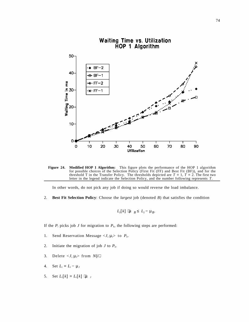
74

Figure 24. Modified HOP 1 Algorithm: This figure plots the performance of the HOP 1 algorithmfor possible choices of the Selection Policy (First Fit (FF) and Best Fit (BF)), and for thethreshold T in the Transfer Policy. The thresholds depicted are T = 1, T = 2. The first twoletter in the legend indicate the Selection Policy, and the number following represents T .

In other words, do not pick any job if doing so would reverse the load imbalance.

2. Best Fit Selection Policy: Choose the largest job (denoted B) that satisfies the condition

Li[k] + µB ≤ Li − µB.

If the Pi picks job J for migration to Pk, the following steps are performed:

1. Send Reservation Message <J, µJ> to Pk.

2. Initiate the migration of job J to Pk.

3. Delete <J, µJ> from N(i).

4. Set Li = Li − µ J

5. Set Li[k] = Li[k] + µ J

75

The HOP 1 algorithm is invoked at Pi when one of the following events occurs: 1) A local job

arrival, 2) A Reservation Message arrival, 3) A job completion, or 4) A migrating job arrival. The

HOP 1 algorithm executes repeatedly until no further migrations are possible. This means that ei-

ther #(N(i)) < T or Pi is less loaded than its neighbors. The algorithm also stops if no job can be

migrated without reversing the load imbalance.

The modified HOP 1 algorithm was simulated in the same distributed system as the load balancing

economy. Figure 24 on page 74 plots the performance of the modified HOP 1 for the following

choice of parameters:

1. Best Fit, T = 1 (BF-1)

2. Best Fit, T = 2 (BF-2)

3. First Fit, T = 1 (FF-1)

4. First Fit, T = 2 (FF-2)

The best choice is Best Fit with transfer threshold T = 1. This is the choice of values that was used

in the previous performance comparisons with the load balancing economy. The performance of

the load balancing economy for all choices of preferences and auction models is competitive with

(or better than) the best choice of parameters for the modified HOP 1 algorithm. Other choices

of parameters for HOP 1 yield performance worse than all 6 combinations of preference relations

and auction models for the load balancing economy.

76

4.0 The Flow Control Economy

This chapter presents an economy that implements flow control in a virtual circuit based computer

network. The agents in this economy are the virtual circuits (VCs) competing for communication

resources and the link controllers that set the prices for these resources. We present decentralized,

synchronous behavior algorithms for the agents in our economy. The allocation of resources to

VC agents computed by these algorithms is proven to be Pareto-optimal [40]. This is a new defi-

nition of optimality for the flow control problem and we discuss the benefits of this definition.

One of the goals of flow control is to fairly allocate communication resources to VCs [9].

Pareto-optimality provides a new definition for fair allocations of link capacity to virtual circuits.

We present a formalization for fairness definitions, and we compare previous definitions to

Pareto-optimality. We prove the existence of a Pareto-optimal allocation for arbitrary networks.

Finally, the results of a simulation study of the convergence behavior of the economy are presented.

This study demonstrates that the economy rapidly converges to a Pareto-optimal allocation over a

broad range of parameters for realistically large networks.

This chapter is structured as follows. Section 1 presents the network model used. This section also

describes the economy in detail. Section 2 proves that the flow control economy computes

Pareto-optimal allocations of link capacity to VCs. Additionally, this section presents a

formalization for defining fair resource allocations and compares the economy to previous work

with respect to fairness. Section 3 uses concepts from mathematical economics to prove the exist-

ence of a feasible, Pareto-optimal allocation for arbitrary flow control economies. In section 4, the

results of an extensive simulation study measuring the economy′s convergence to optimal allo-

cations are presented. Section 5 compares the economy to previous work on flow control, and

section 6 is a conclusion. Several lemmas used in the proofs of this chapter′s theorems are proved

in an appendix.

4.1 Network and Economy

In this section, we define the network model and the economy. Model the network as a graph

G = < V , E> , where V = {1, 2, ... , K} is a set of nodes and E = {1, 2, ... , M} is the set of edges re-

presenting the network links. We associate two numbers with each edge i ∈ E: A capacity Ci

(measured in data units per second), and a link supply Si such that Si < Ci. The link supply sets an

77

upper bound on the link utilization to assure that the queuing delays are bounded. This does not

limit generality because Si arbitrarily close to Ci is allowed. The goal of the flow control economy

is to allocate the link supplies among virtual circuits (VCs).

Let A = {1, 2, ... , N} denote the set of VCs. For each VC a ∈ A there is an associated path of edges

in G,

Pa = la,1, la,2, ... , la, m(a), with la, i ∈ E.

VCs play the roles of consumer agents in the economy and seek allocations of link capacities. An

allocation of capacity is a vector x• = < x1, x2, ... , xM>, such that xi ≥ 0. Each link i ∈ E has a sup-

plier agent (network node) that charges VCs using i. A price system is a vector

p• = < p1, p2, ... , pM> , where pi ≥ ε > 0. We restrict prices to be strictly positive in order to avoid

pathological behaviors. The assumption that pi > 0 is used in later sections. This assumption does

not limit generality because pi arbitrarily small is permitted.

Each VC a has a binary preference relation [40] denoted • a over the allocations; x• • a y

• denotes

that VC a prefers allocation x•

at least as much as allocation y•

. If x• • a y

• and y

• • a x•

, VC a is in-

different between x•

and y•

(denoted x• ∼ a y

•). If x

• • a y•

but not x• ∼ a y

•, then VC a strictly prefers

x•

(x• • a y

•).

We define • a to reflect two features of an allocation x•

: Its throughput T(x• ) and its worst case

average delay D(x• ). A VC a attempts to maximize T(x

• ) until it reaches its individual throughput

goal γa chosen by the VC′s user, and then tries to minimize D(x• ). The relation • a is defined to

capture this goal as follows:

1. If T(x• ) ≤ γa and T(y• ) ≤ γa, then if T(y• ) ≥ T(x

• ), y• • a x

•.

2. If T(x• ) < γa and T(y• ) ≥ γa, then y

• • a x•

.

3. If T(x• ) ≥ γa and T(y• ) ≥ γa, then if D(x

• ) ≥ D(y• ), y• • a x

•.

This preference relation can be tailored to model the diversity of throughput-delay goals in a com-

puter network supporting many types of VCs. A circuit supporting a throughput oriented applica-

tion (e.g. - file transfer) is modeled by setting γa = ∞ . The preference relation also models

applications with low throughput demands and tight delay constraints such as a VC connecting a

workstation to a database. In this case, the throughput goal γa is the mean transaction

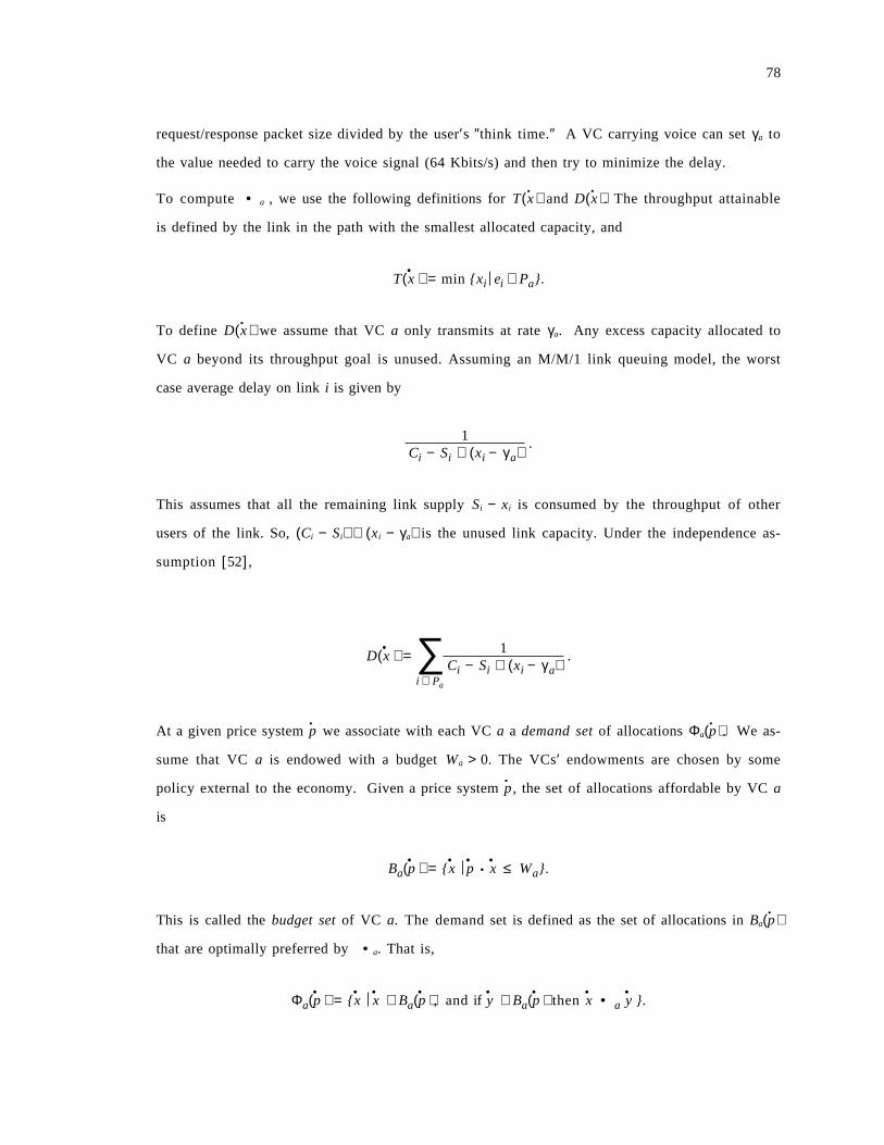
78

request/response packet size divided by the user′s ″think time.″ A VC carrying voice can set γa to

the value needed to carry the voice signal (64 Kbits/s) and then try to minimize the delay.

To compute • a , we use the following definitions for T(x• ) and D(x

• ). The throughput attainable

is defined by the link in the path with the smallest allocated capacity, and

T(x• ) = min {xi ei ∈ Pa}.

To define D(x• ) we assume that VC a only transmits at rate γa. Any excess capacity allocated to

VC a beyond its throughput goal is unused. Assuming an M/M/1 link queuing model, the worst

case average delay on link i is given by

1Ci − Si + (xi − γa)

.

This assumes that all the remaining link supply Si − xi is consumed by the throughput of other

users of the link. So, (Ci − Si) + (xi − γa) is the unused link capacity. Under the independence as-

sumption [52],

D(x• ) = ∑

i ∈ Pa

1Ci − Si + (xi − γa)

.

At a given price system p•

we associate with each VC a a demand set of allocations Φa(p• ). We as-

sume that VC a is endowed with a budget Wa > 0. The VCs′ endowments are chosen by some

policy external to the economy. Given a price system p•

, the set of allocations affordable by VC a

is

Ba(p• ) = {x•

p•

• x• ≤ Wa}.

This is called the budget set of VC a. The demand set is defined as the set of allocations in Ba(p• )

that are optimally preferred by • a. That is,

Φa(p• ) = {x•

x• ∈ Ba(p• ), and if y

• ∈ Ba(p• ) then x• • a y

•}.

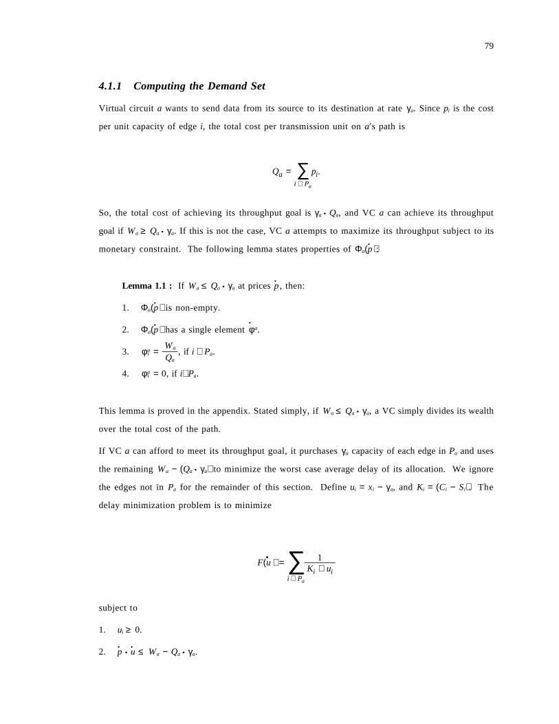
79

4.1.1 Computing the Demand Set

Virtual circuit a wants to send data from its source to its destination at rate γa. Since pi is the cost

per unit capacity of edge i, the total cost per transmission unit on a′s path is

Qa = ∑i ∈ Pa

pi.

So, the total cost of achieving its throughput goal is γa • Qa, and VC a can achieve its throughput

goal if Wa ≥ Qa • γa. If this is not the case, VC a attempts to maximize its throughput subject to its

monetary constraint. The following lemma states properties of Φa(p• ):

Lemma 1.1 : If Wa ≤ Qa • γa at prices p•

, then:

1. Φa(p• ) is non-empty.

2. Φa(p• ) has a single element φ

•a.

3. φ ai =

Wa

Qa, if i ∈ Pa.

4. φ ai = 0, if i∉Pa.

This lemma is proved in the appendix. Stated simply, if Wa ≤ Qa • γa, a VC simply divides its wealth

over the total cost of the path.

If VC a can afford to meet its throughput goal, it purchases γa capacity of each edge in Pa and uses

the remaining Wa − (Qa • γa) to minimize the worst case average delay of its allocation. We ignore

the edges not in Pa for the remainder of this section. Define ui = xi − γa, and Ki = (Ci − Si). The

delay minimization problem is to minimize

F(u• ) = ∑i ∈ Pa

1Ki + ui

subject to

1. ui ≥ 0.

2. p•

• u• ≤ Wa − Qa • γa.

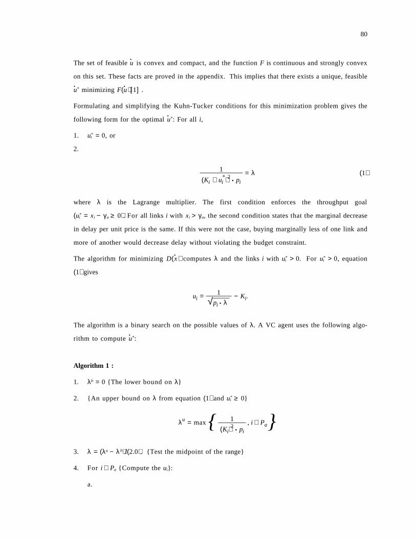
80

The set of feasible u•

is convex and compact, and the function F is continuous and strongly convex

on this set. These facts are proved in the appendix. This implies that there exists a unique, feasible

u• * minimizing F(u• )[1] .

Formulating and simplifying the Kuhn-Tucker conditions for this minimization problem gives the

following form for the optimal u• *: For all i,

1. u*i = 0, or

2.

1

(Ki + u*i )2

• pi

= λ (1)

where λ is the Lagrange multiplier. The first condition enforces the throughput goal

(u*i = xi − γ a ≥ 0). For all links i with xi > γa, the second condition states that the marginal decrease

in delay per unit price is the same. If this were not the case, buying marginally less of one link and

more of another would decrease delay without violating the budget constraint.

The algorithm for minimizing D(x• ) computes λ and the links i with u*

i > 0. For u*i > 0, equation

(1) gives

ui = 1

√pi • λ− Ki.

The algorithm is a binary search on the possible values of λ. A VC agent uses the following algo-

rithm to compute u• *:

Algorithm 1 :

1. λb = 0 {The lower bound on λ}

2. {An upper bound on λ from equation (1) and u*i ≥ 0}

λu = max { 1

(Ki)2

• pi

, i ∈ Pa}3. λ = (λu − λb)/(2.0). {Test the midpoint of the range}

4. For i ∈ Pa {Compute the ui}:

a.

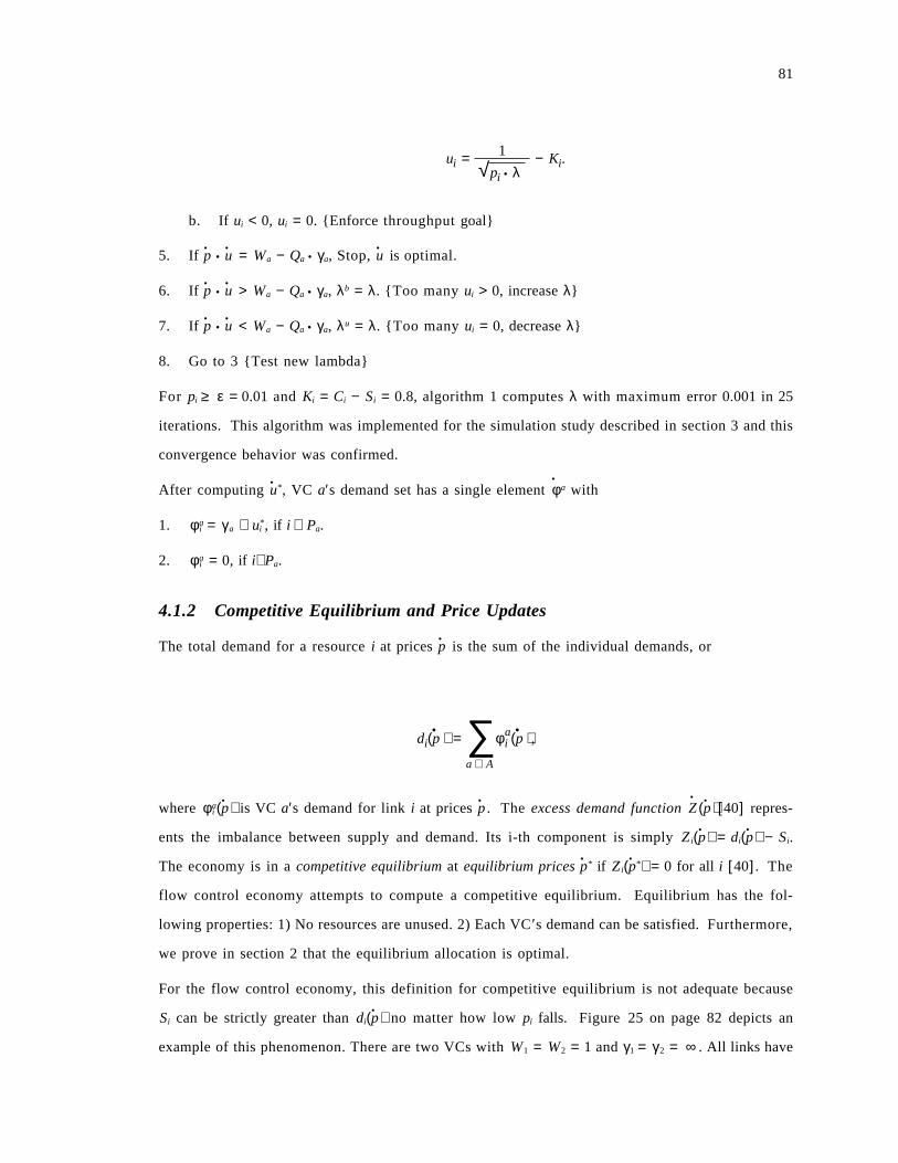
81

ui = 1

√pi • λ− Ki.

b. If ui < 0, ui = 0. {Enforce throughput goal}

5. If p•

• u• = Wa − Qa • γa, Stop, u

•is optimal.

6. If p•

• u• > Wa − Qa • γa, λb = λ. {Too many ui > 0, increase λ}

7. If p•

• u• < Wa − Qa • γa, λu = λ. {Too many ui = 0, decrease λ}

8. Go to 3 {Test new lambda}

For pi ≥ ε = 0.01 and Ki = Ci − Si = 0.8, algorithm 1 computes λ with maximum error 0.001 in 25

iterations. This algorithm was implemented for the simulation study described in section 3 and this

convergence behavior was confirmed.

After computing u• *, VC a′s demand set has a single element φ

•a with

1. φ ai = γ a + u*

i , if i ∈ Pa.

2. φ ai = 0, if i∉Pa.

4.1.2 Competitive Equilibrium and Price Updates

The total demand for a resource i at prices p•

is the sum of the individual demands, or

di(p• ) = ∑

a ∈ A

φai (p• ),

where φ ai (p

• ) is VC a′s demand for link i at prices p•

. The excess demand function Z•

(p• )[40] repres-

ents the imbalance between supply and demand. Its i-th component is simply Z i(p• ) = di(p

• ) − Si.

The economy is in a competitive equilibrium at equilibrium prices p• * if Z i(p

• *) = 0 for all i [40]. The

flow control economy attempts to compute a competitive equilibrium. Equilibrium has the fol-

lowing properties: 1) No resources are unused. 2) Each VC ′s demand can be satisfied. Furthermore,

we prove in section 2 that the equilibrium allocation is optimal.

For the flow control economy, this definition for competitive equilibrium is not adequate because

Si can be strictly greater than di(p• ) no matter how low pi falls. Figure 25 on page 82 depicts an

example of this phenomenon. There are two VCs with W1 = W2 = 1 and γ1 = γ 2 = ∞ . All links have

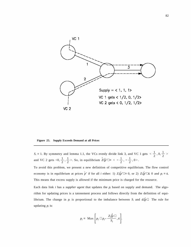
82

Figure 25. Supply Exceeds Demand at all Prices

Si = 1. By symmetry and lemma 1.1, the VCs evenly divide link 3, and VC 1 gets < 12

, 0, 12

>

and VC 2 gets <0, 12

, 12

>. So, in equilibrium Z•

(p• *) = < − 12

, − 12

, 0 > .

To avoid this problem, we present a new definition of competitive equilibrium. The flow control

economy is in equilibrium at prices p• * if for all i either: 1) Z i(p

• *) = 0, or 2) Z i(p• *) ≤ 0 and pi = ε.

This means that excess supply is allowed if the minimum price is charged for the resource.

Each data link i has a supplier agent that updates the pi based on supply and demand. The algo-

rithm for updating prices is a tatonement process and follows directly from the definition of equi-

librium. The change in pi is proportional to the imbalance between Si and di(p• ). The rule for

updating pi is:

pi = Max pi + pi •Zi(p

• )Si

, ε .

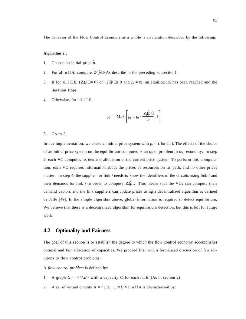
83

The behavior of the Flow Control Economy as a whole is an iteration described by the following:

Algorithm 2 :

1. Choose an initial price p•

.

2. For all a ∈ A, compute φ•

a(p• ) {As describe in the preceding subsection}.

3. If for all i ∈ E, (Z i(p• ) = 0) or ( Z i(p

• ) ≤ 0 and pi = ε), an equilibrium has been reached and the

iteration stops.

4. Otherwise, for all i ∈ E,

pi = Max pi + pi •Zi(p

• )Si

, ε .

5. Go to 2.

In our implementation, we chose an initial price system with pi = ε for all i. The effects of the choice

of an initial price system on the equilibrium computed is an open problem in our economy. In step

2, each VC computes its demand allocation at the current price system. To perform this computa-

tion, each VC requires information about the prices of resources on its path, and no other prices

matter. In step 4, the supplier for link i needs to know the identifiers of the circuits using link i and

their demands for link i in order to compute Z i(p• ). This means that the VCs can compute their

demand vectors and the link suppliers can update prices using a decentralized algorithm as defined

by Jaffe [49]. In the simple algorithm above, global information is required to detect equilibrium.

We believe that there is a decentralized algorithm for equilibrium detection, but this is left for future

work.

4.2 Optimality and Fairness

The goal of this section is to establish the degree to which the flow control economy accomplishes

optimal and fair allocation of capacities. We proceed first with a formalized discussion of fair sol-

utions to flow control problems.

A flow control problem is defined by:

1. A graph G = < V ,E> with a capacity Ci for each i ∈ E. (As in section 2)

2. A set of virtual circuits A = {1, 2, ... , N} . VC a ∈ A is characterized by:

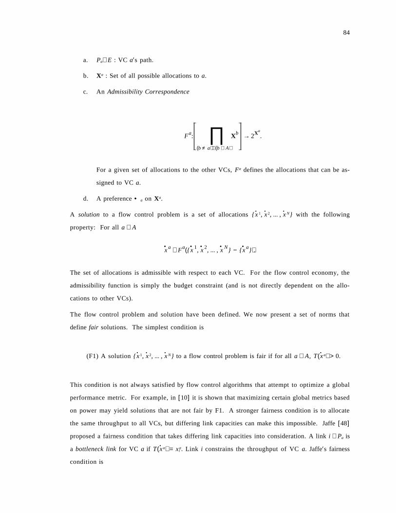
84

a. Pa⊆E : VC a′s path.

b. Xa : Set of all possible allocations to a.

c. An Admissibility Correspondence

Fa: ∏(b ≠ a)∧(b ∈ A)

Xb → 2Xa

.

For a given set of allocations to the other VCs, Fa defines the allocations that can be as-

signed to VC a.

d. A preference • a on Xa.

A solution to a flow control problem is a set of allocations {x• 1, x

• 2, ... , x• N} with the following

property: For all a ∈ A

x• a ∈ Fa({x

• 1, x• 2, ... , x• N} − {x

• a}).

The set of allocations is admissible with respect to each VC. For the flow control economy, the

admissibility function is simply the budget constraint (and is not directly dependent on the allo-

cations to other VCs).

The flow control problem and solution have been defined. We now present a set of norms that

define fair solutions. The simplest condition is

(F1) A solution {x• 1, x

• 2, ... , x• N} to a flow control problem is fair if for all a ∈ A, T(x

• a) > 0.

This condition is not always satisfied by flow control algorithms that attempt to optimize a global

performance metric. For example, in [10] it is shown that maximizing certain global metrics based

on power may yield solutions that are not fair by F1. A stronger fairness condition is to allocate

the same throughput to all VCs, but differing link capacities can make this impossible. Jaffe [48]

proposed a fairness condition that takes differing link capacities into consideration. A link i ∈ Pa is

a bottleneck link for VC a if T(x• a) = x a

i . Link i constrains the throughput of VC a. Jaffe′s fairness

condition is

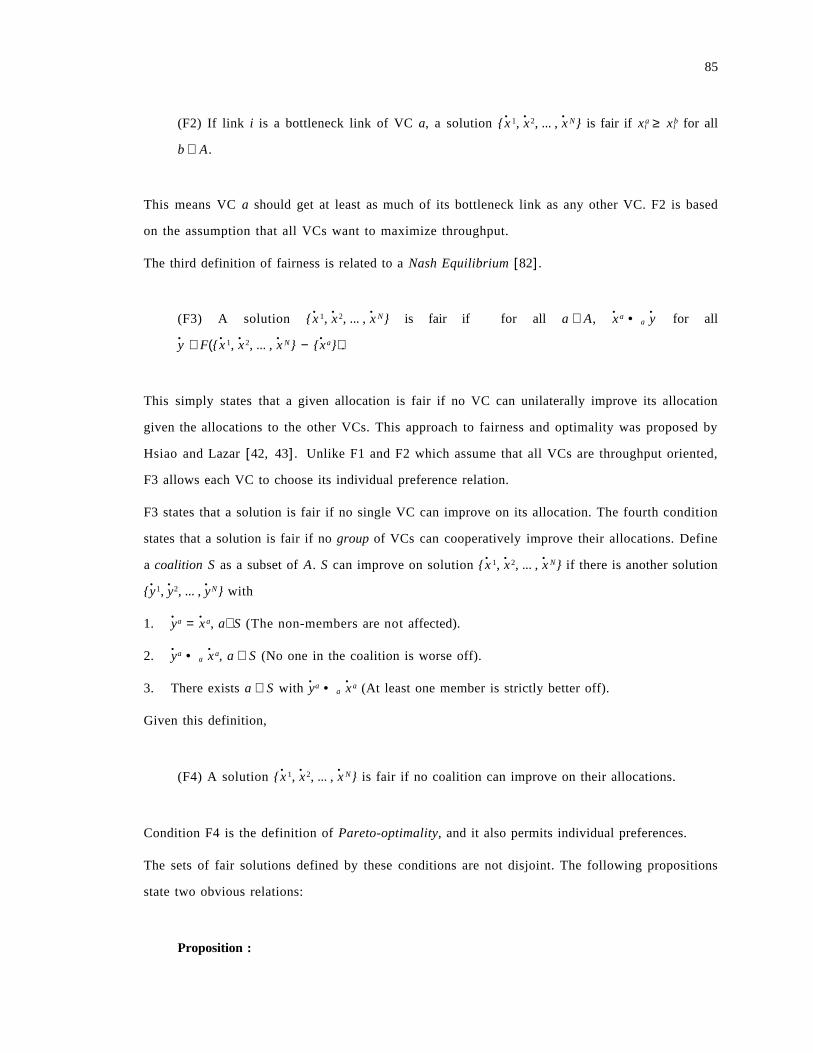
85

(F2) If link i is a bottleneck link of VC a, a solution {x• 1, x

• 2, ... , x• N} is fair if x a

i ≥ x bi for all

b ∈ A.

This means VC a should get at least as much of its bottleneck link as any other VC. F2 is based

on the assumption that all VCs want to maximize throughput.

The third definition of fairness is related to a Nash Equilibrium [82].

(F3) A solution {x• 1, x

• 2, ... , x• N} is fair if for all a ∈ A, x

• a • a y•

for all

y• ∈ F({x

• 1, x• 2, ... , x• N} − {x

• a}).

This simply states that a given allocation is fair if no VC can unilaterally improve its allocation

given the allocations to the other VCs. This approach to fairness and optimality was proposed by

Hsiao and Lazar [42, 43]. Unlike F1 and F2 which assume that all VCs are throughput oriented,

F3 allows each VC to choose its individual preference relation.

F3 states that a solution is fair if no single VC can improve on its allocation. The fourth condition

states that a solution is fair if no group of VCs can cooperatively improve their allocations. Define

a coalition S as a subset of A. S can improve on solution {x• 1, x

• 2, ... , x• N} if there is another solution

{y• 1, y

• 2, ... , y• N} with

1. y• a = x

• a, a∉S (The non-members are not affected).

2. y• a • a x

• a, a ∈ S (No one in the coalition is worse off).

3. There exists a ∈ S with y• a • a x

• a (At least one member is strictly better off).

Given this definition,

(F4) A solution {x• 1, x

• 2, ... , x•

N} is fair if no coalition can improve on their allocations.

Condition F4 is the definition of Pareto-optimality, and it also permits individual preferences.

The sets of fair solutions defined by these conditions are not disjoint. The following propositions

state two obvious relations:

Proposition :

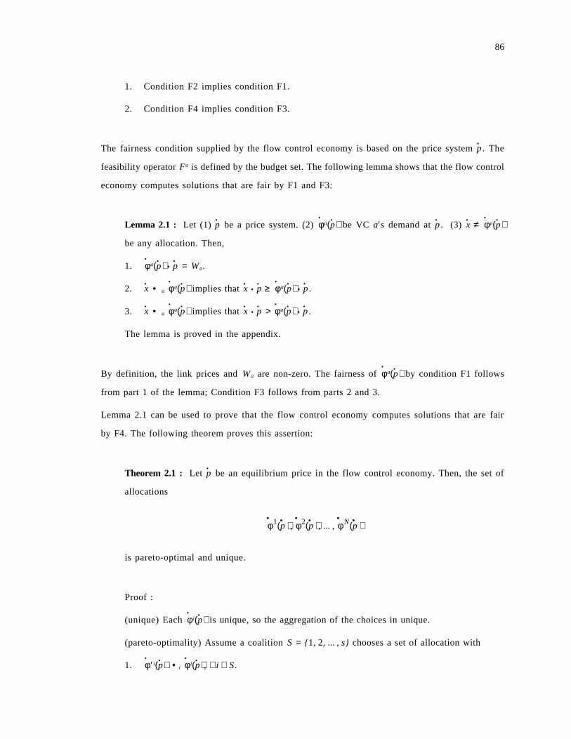
86

1. Condition F2 implies condition F1.

2. Condition F4 implies condition F3.

The fairness condition supplied by the flow control economy is based on the price system p•

. The

feasibility operator Fa is defined by the budget set. The following lemma shows that the flow control

economy computes solutions that are fair by F1 and F3:

Lemma 2.1 : Let (1) p•

be a price system. (2) φ•

a(p• ) be VC a′s demand at p•

. (3) x• ≠ φ

•a(p• )

be any allocation. Then,

1. φ•

a(p• ) • p• = Wa.

2. x• • a φ

•a(p• ) implies that x

•• p

• ≥ φ•

a(p• ) • p•

.

3. x• • a φ

•a(p• ) implies that x

•• p

• > φ•

a(p• ) • p•

.

The lemma is proved in the appendix.

By definition, the link prices and Wa are non-zero. The fairness of φ•

a(p• ) by condition F1 follows

from part 1 of the lemma; Condition F3 follows from parts 2 and 3.

Lemma 2.1 can be used to prove that the flow control economy computes solutions that are fair

by F4. The following theorem proves this assertion:

Theorem 2.1 : Let p•

be an equilibrium price in the flow control economy. Then, the set of

allocations

φ• 1(p• ), φ

• 2(p• ), ... , φ• N(p• )

is pareto-optimal and unique.

Proof :

(unique) Each φ•

i(p• ) is unique, so the aggregation of the choices in unique.

(pareto-optimality) Assume a coalition S = {1, 2, ... , s} chooses a set of allocation with

1. φ•

′ i(p• ) • i φ•

i(p• ), ∀i ∈ S.

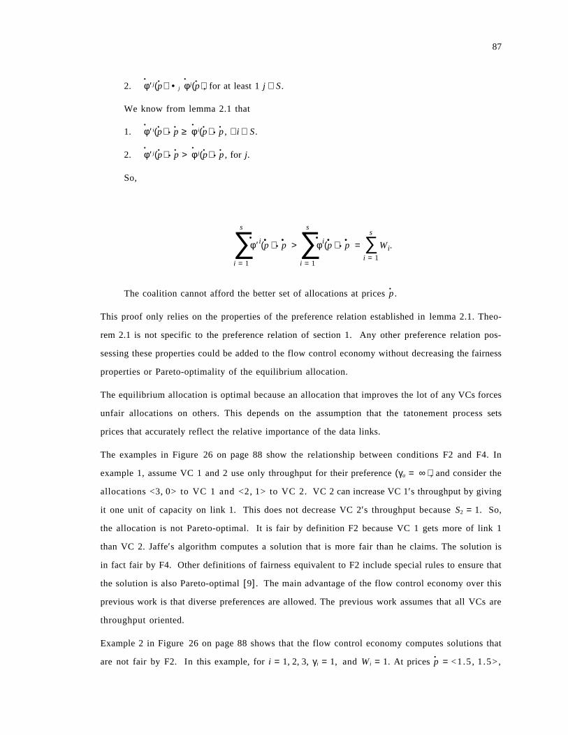
87

2. φ•

′ j(p• ) • j φ•

j(p• ), for at least 1 j ∈ S.

We know from lemma 2.1 that

1. φ•

′ i(p• ) • p• ≥ φ

•i(p• ) • p

•, ∀i ∈ S.

2. φ•

′ j(p• ) • p• > φ

•j(p• ) • p

•, for j.

So,

∑s

i = 1

φ•

′i(p• ) • p• > ∑

s

i = 1

φ• i(p• ) • p

• = ∑s

i = 1

Wi.

The coalition cannot afford the better set of allocations at prices p•

.

This proof only relies on the properties of the preference relation established in lemma 2.1. Theo-

rem 2.1 is not specific to the preference relation of section 1. Any other preference relation pos-

sessing these properties could be added to the flow control economy without decreasing the fairness

properties or Pareto-optimality of the equilibrium allocation.

The equilibrium allocation is optimal because an allocation that improves the lot of any VCs forces

unfair allocations on others. This depends on the assumption that the tatonement process sets

prices that accurately reflect the relative importance of the data links.

The examples in Figure 26 on page 88 show the relationship between conditions F2 and F4. In

example 1, assume VC 1 and 2 use only throughput for their preference (γa = ∞ ), and consider the

allocations <3, 0> to VC 1 and <2, 1> to VC 2. VC 2 can increase VC 1′s throughput by giving

it one unit of capacity on link 1. This does not decrease VC 2′s throughput because S2 = 1. So,

the allocation is not Pareto-optimal. It is fair by definition F2 because VC 1 gets more of link 1

than VC 2. Jaffe′s algorithm computes a solution that is more fair than he claims. The solution is

in fact fair by F4. Other definitions of fairness equivalent to F2 include special rules to ensure that

the solution is also Pareto-optimal [9]. The main advantage of the flow control economy over this

previous work is that diverse preferences are allowed. The previous work assumes that all VCs are

throughput oriented.

Example 2 in Figure 26 on page 88 shows that the flow control economy computes solutions that

are not fair by F2. In this example, for i = 1, 2, 3, γi = 1, and W i = 1. At prices p• = <1.5 , 1 .5>,

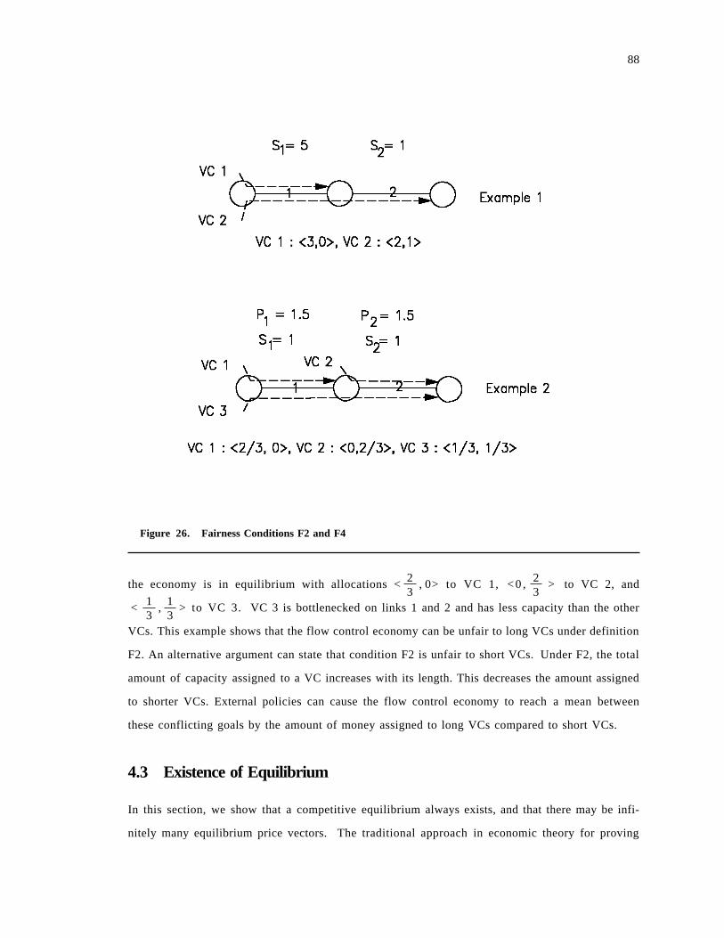
88

Figure 26. Fairness Conditions F2 and F4

the economy is in equilibrium with allocations < 23

, 0> to VC 1, < 0 , 23

> to VC 2, and

< 13

, 13

> to VC 3. VC 3 is bottlenecked on links 1 and 2 and has less capacity than the other

VCs. This example shows that the flow control economy can be unfair to long VCs under definition

F2. An alternative argument can state that condition F2 is unfair to short VCs. Under F2, the total

amount of capacity assigned to a VC increases with its length. This decreases the amount assigned

to shorter VCs. External policies can cause the flow control economy to reach a mean between

these conflicting goals by the amount of money assigned to long VCs compared to short VCs.

4.3 Existence of Equilibrium

In this section, we show that a competitive equilibrium always exists, and that there may be infi-

nitely many equilibrium price vectors. The traditional approach in economic theory for proving

89

the existence of an equilibrium price vector is based on fixed point theorems [1, 5, 40]. A point

p• 0 is a fixed point of a function f

• if f(p• 0) = p

• 0. A function f•

(p• ) = p• + Z

•(p• ) is defined and shown to

have a fixed point p• 0. This implies that Z

•(p• 0) = 0 and p

• 0 is an equilibrium price vector.

We must modify these tools to prove existence of equilibrium in the flow control economy because

of the non-standard definition of equilibrium that may have Z•

(p• *) ≠ 0•

in equilibrium. Economic

theory also assumes that the demand functions of the individual agents are continuous with p•

. We

cannot make this assumption, and we prove that the demand function defined in section 1 is con-

tinuous.

We define a new function H•

(p• ) with the property that H•

(p• ) = 0•

if, and only if, p•

is an equilibrium

price system. We then show that f•

(p• ) = p• + H

•(p• ) has a fixed point.

We define the function H•

(p• ) with i-th component

Hi(p• ) = (pi − ε) • Zi(p

• ) + Zi(p• ) + Zi(p

• ) .

By our definition of equilibrium, if p• * is an equilibrium price vector, then for every i

1. Z i(p• *) = 0, or

2. pi = ε and Z i(p• *) ≤ 0.

If Z i(p• *) = 0, then Hi(p

• *) = 0. If pi = ε, then the first term in Hi(p• *) is 0. If Z i(p

• *) ≤ 0, then the second

and third terms cancel and Hi(p• *) = 0. So, if p

• * is an equilibrium price, Hi(p• *) = 0 for all i, which

implies H•

(p• *) = 0•

.

Assume that H•

(p• ) = 0•

. We must show that p•

is an equilibrium price vector. We know by definition

that pi − ε ≥ 0. So, Hi(p• ) = 0 implies that Z i(p

• ) ≤ 0. This, in turn, implies that

Hi(p• ) = (pi − ε) • Zi(p

• ).

This term is 0 only if Z i(p• ) = 0 or pi = ε. So, Hi(p

• ) = 0 implies that Z i(p• ) = 0 or Z i(p

• ) ≤ 0 and

pi = ε. The following theorem has been shown.

Theorem 3.1 : H•

(p• ) = 0•

if, and only if, p•

is an equilibrium price vector.

Define the function f•

(p• ) = p• + H

•(p• ). We apply the following theorem to show that f

• has a fixed

point.

90

(Brouwer′s fixed point) Theorem : Let X be a compact, convex subset of • M, and let f•

be a

continuous function mapping X into X. Then there exists x• 0 ∈ X such that f

•(x

• 0) = x• 0.

Brouwer′s theorem is discussed in economic contexts in [1, 5, 40].

To apply the fixed point theorem, we must

1. Define the set X.

2. Prove f•

maps X into itself.

3. Prove continuity of f•

on X.

Let W T = ∑N

i = 1

W i. This is the total amount of money possessed by the VCs. Define the set X as

X = {x• ε ≤ xi ≤

2WTε }.

X is simply a cube in • M and contains its boundary. So, it is is compact and convex.

We must show that f(p• ) ∈ X for all p• ∈ X. To do so, we make two assumptions that do not limit

generality. First, we assume that 0 ≤ Si ≤ 1 for all i. If this is not the case, an equivalent economy

can be created by dividing all Si by Max {Si 1 ≤ i ≤ M} . Secondly, we assume that ε ≤ Si for all i.

This is possible because the only constraint is ε > 0.

Since pi ≥ ε > 0, fi takes its minimal value at p• 0 when Z i(p

• )0 is minimal. Our assumptions that

Si ≤ 1 implies that Z i(p• ) ≥ − 1, and we have

fi(p• 0) ≥ p0

i + (p• 0i − ε) • ( − 1) + ( − 1) + − 1 = ε.

To prove that fi(p• ) ≤

2W T

ε we define a function

g(pi) = pi + (pi − ε)WTpi

+2WT

pi.

The budget constraint implies that Z i(p• 0) ≤

W T

p0i

− Si. We know that Si > 0 and we have

g(p0i ) ≥ fi(p0

i ). The second derivative of g(p• ) is

g′′(p• ) =2(2 − ε)WT

p3i

,

91

which is strictly positive on ε,2W T

ε provided that ε < 2. So, g(pi) takes its maximal value at ei-

ther pi = ε or pi =2W T

ε . At pi = ε,

fi(p• 0) ≤ ε +

2WTε − 2Si ≤

2WTε .

At p0i =

2W T

ε , Z i(p• 0) ≤ 0 because of the budget constraint and

fi(p• 0) ≤

2WTε .

This shows that for all p• ∈ X, ε ≤ fi(p

• ) ≤2W T

ε for all i which means that f•

(p• ) ∈ X. So, f•

maps X

into itself.

The function H•

(p• ) is continuous if the excess demand function Z•

(p• ) is continuous. The excess de-

mand function is simply

Z•

(p• ) =(∑N

i = 1

φ• i(p• ))− S

•,

where φ•

a(p• ) is VC a′s demand at p•

and S•

is the vector of link supplies. We will show that φ•

a(p• ) is

continuous, which implies continuity of Z•

.

Lemma 1.1 shows that for VC a, if

γa ∑j ∈ Pa

pj ≥ Wa

the agent′s demand is a continuous function of p•

. If the agent can afford its throughput goal, and

attempts to minimize delay, we have to show that the u• * solving the minimization problem in the

previous section is a continuous function of p•

.

Let U(p• ) be defined as follows: u• ∈ • M is in U(p• ) if,

1. ui ≥ 0

2.

92

∑j ∈ Pa

(pi • ui) ≤ Wa − (γa) ∑j ∈ Pa

pi.

Define the function F:U(p• ) → • as

F(u• ) = ∑i ∈ Pa

1(Ki + ui)

as in section 2.

The following lemmas are needed to prove continuity and are proved in this chapter ′s appendix.

Lemmas 3 :

1. For any p•

, F is continuous and strongly convex on U(p• ).

2. For any p•

, U(p• ) is compact and convex.

3. A sequence of points {x• m} in • N converges to x

• 0 if, and only if, every sub sequence

{x• mk} contains a subsequence {x

• m′k} that converges to x• 0.

We prove the following theorem:

Theorem 3.2 : For all p•

, let x• = M(p• ) denote a vector in U(p• ) minimizing F(x

• ). Then M(p• )

is a continuous function of p•

.

Proof:

1. M(p• ) is a function:

a. U(p• ) is compact, and F is continuous on U(p• ), so there exists an x• ∈ U(p• ) mini-

mizing F [1].

b. So M(p• ) is defined for all p•

.

93

c. Furthermore, convexity of U(p• ) and strong convexity of F on U(p• ) imply that x•

is

unique for any p•

.

d. So, M is not multivalued and is a function.

2. M(p• ) is continuous:

a. Pick a point p• 0. Let p

• m be a sequence converging to p• 0.

b. Denote x• m = M(p• m) and x

• 0 = M(p• 0).

c. We must show that as p• m → p

• 0, x• m → x

• 0.

d. Define two sequences w• m and u

• m with the following properties:

1) w• m:

a) w• m ∈ U(p• m).

b) For all z• ∈ U(p• m),

w• m − x

• 0 ≤ z• − x

• 0 .

w• m is the point in U(p• m) closest to x

• 0.

2) u• m:

a) u• m ∈ U(p• 0).

b) For all y• ∈ U(p• 0),

u• m − x

• m ≤ y• − x

• m .

u• m is the point in U(p• 0) closest to x

• m.

u•

m and w•

m exist because U(p• m) and U(p• 0) are compact. Figure 27 on page 94 shows

an example of the sequences x• m, w

• m, u• m and their relationship to p

• 0 and x• 0 in the two

dimensional case.

e. As p•

m → p• 0,

1) w• m − x

• 0 → 0

2) u• m − x

• m → 0.

This is intuitively clear. It is formally proved in an appendix to this chapter.

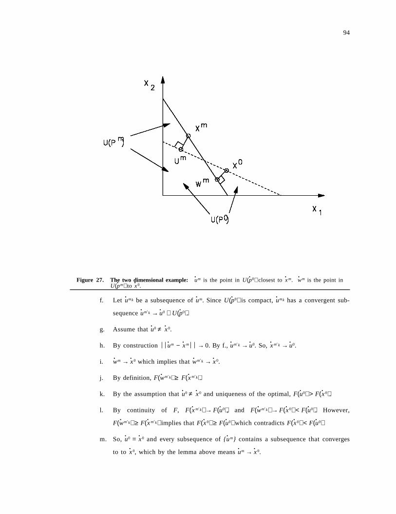
94

Figure 27. The two dimensional example: u• m is the point in U(p• 0) closest to x

• m. w• m is the point in

U(p• m) to x• 0.

f. Let u• mk be a subsequence of u

• m. Since U(p• 0) is compact, u• mk has a convergent sub-

sequence u• m′k → u

• 0 ∈ U(p• 0).

g. Assume that u• 0 ≠ x

• 0.

h. By construction u• m − x

• m → 0. By f., u• m′k → u

• 0. So, x• m′k → u

• 0.

i. w•

m → x• 0 which implies that w

•m′k → x

• 0.

j. By definition, F(w• m′k) ≥ F(x• m′k).

k. By the assumption that u• 0 ≠ x

• 0 and uniqueness of the optimal, F(u• 0) > F(x• 0).

l. By continuity of F, F(x• m′k) → F(u• 0), and F(w• m′k) → F(x

• 0) < F(u• 0). However,

F(w• m′k) ≥ F(x• m′k) implies that F(x

• 0) ≥ F(u• 0) which contradicts F(x• 0) < F(u• 0)

m. So, u• 0 = x

• 0 and every subsequence of {u• m} contains a subsequence that converges

to to x• 0, which by the lemma above means u

• m → x• 0.

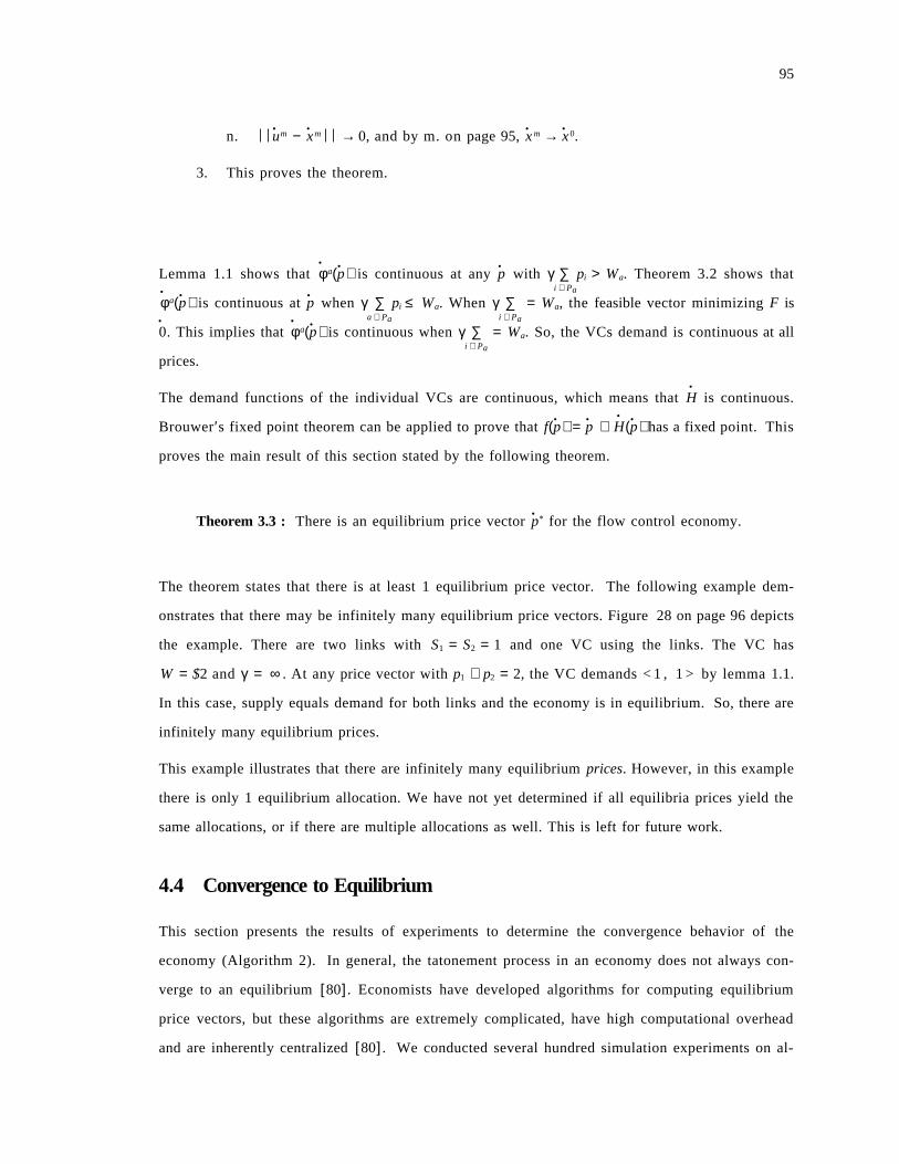
95

n. u• m − x

• m → 0, and by m. on page 95, x• m → x

• 0.

3. This proves the theorem.

Lemma 1.1 shows that φ•

a(p• ) is continuous at any p•

with γ ∑i ∈ Pa

pi > Wa. Theorem 3.2 shows that

φ•

a(p• ) is continuous at p•

when γ ∑a ∈ Pa

pi ≤ Wa. When γ ∑i ∈ Pa

= Wa, the feasible vector minimizing F is

0•

. This implies that φ•

a(p• ) is continuous when γ ∑i ∈ Pa

= Wa. So, the VCs demand is continuous at all

prices.

The demand functions of the individual VCs are continuous, which means that H•

is continuous.

Brouwer′s fixed point theorem can be applied to prove that f(p• ) = p• + H

•(p• ) has a fixed point. This

proves the main result of this section stated by the following theorem.

Theorem 3.3 : There is an equilibrium price vector p• * for the flow control economy.

The theorem states that there is at least 1 equilibrium price vector. The following example dem-

onstrates that there may be infinitely many equilibrium price vectors. Figure 28 on page 96 depicts

the example. There are two links with S1 = S2 = 1 and one VC using the links. The VC has

W = $2 and γ = ∞ . At any price vector with p1 + p2 = 2, the VC demands < 1 , 1 > by lemma 1.1.

In this case, supply equals demand for both links and the economy is in equilibrium. So, there are

infinitely many equilibrium prices.

This example illustrates that there are infinitely many equilibrium prices. However, in this example

there is only 1 equilibrium allocation. We have not yet determined if all equilibria prices yield the

same allocations, or if there are multiple allocations as well. This is left for future work.

4.4 Convergence to Equilibrium

This section presents the results of experiments to determine the convergence behavior of the

economy (Algorithm 2). In general, the tatonement process in an economy does not always con-

verge to an equilibrium [80]. Economists have developed algorithms for computing equilibrium

price vectors, but these algorithms are extremely complicated, have high computational overhead

and are inherently centralized [80]. We conducted several hundred simulation experiments on al-

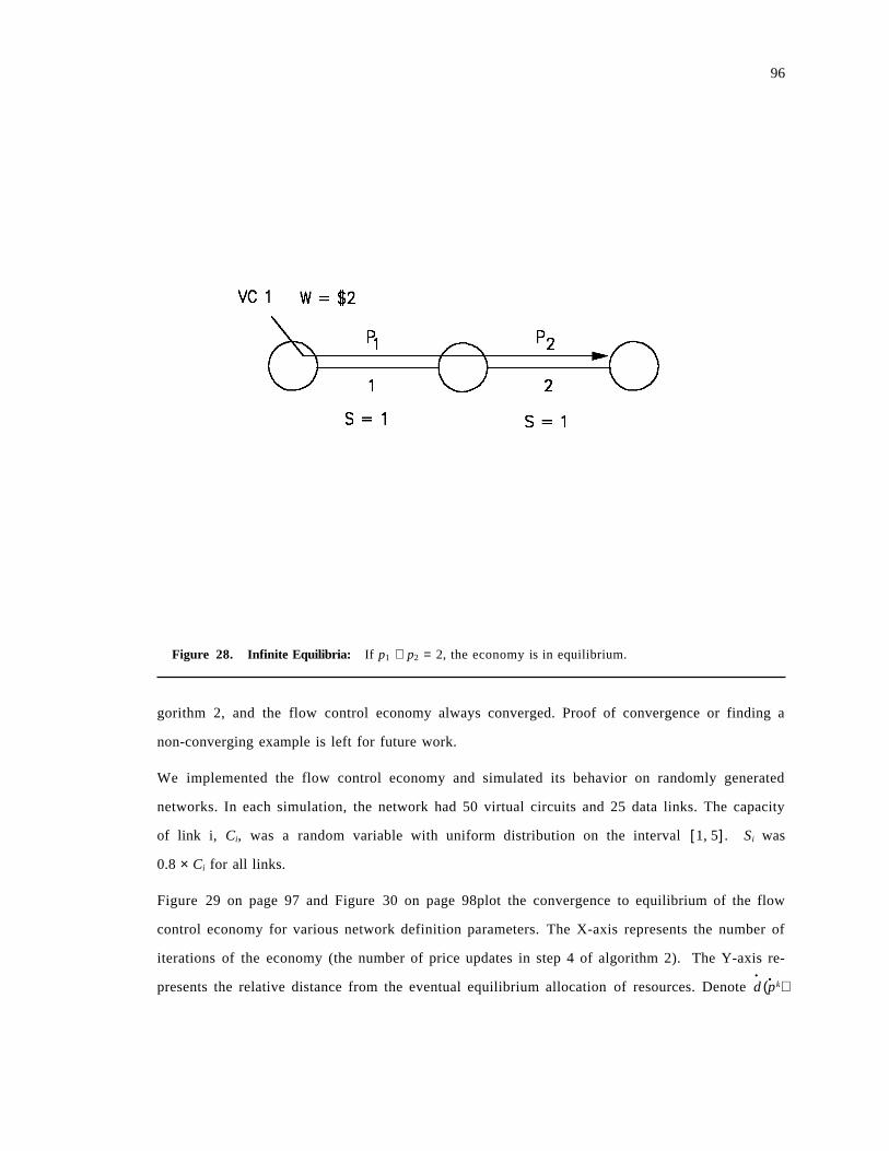
96

Figure 28. Infinite Equilibria: If p1 + p2 = 2, the economy is in equilibrium.

gorithm 2, and the flow control economy always converged. Proof of convergence or finding a

non-converging example is left for future work.

We implemented the flow control economy and simulated its behavior on randomly generated

networks. In each simulation, the network had 50 virtual circuits and 25 data links. The capacity

of link i, Ci, was a random variable with uniform distribution on the interval [1, 5]. Si was

0.8 × Ci for all links.

Figure 29 on page 97 and Figure 30 on page 98plot the convergence to equilibrium of the flow

control economy for various network definition parameters. The X-axis represents the number of

iterations of the economy (the number of price updates in step 4 of algorithm 2). The Y-axis re-

presents the relative distance from the eventual equilibrium allocation of resources. Denote d•

(p• k)

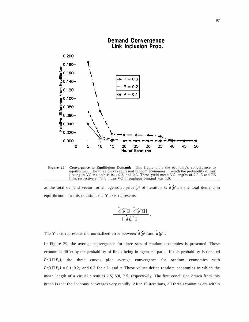
97

Figure 29. Convergence to Equilibrium Demand: This figure plots the economy′s convergence toequilibrium. The three curves represent random economies in which the probability of linki being in VC a′s path is 0.1, 0.2, and 0.3. These yield mean VC lengths of 2.5, 5 and 7.5links respectively. The mean VC throughput demand was 1.0.

as the total demand vector for all agents at price p• k of iteration k; d

•(p• *) is the total demand in

equilibrium. In this notation, the Y-axis represents

d•

(p• *) − d•

(p• k)

d•

(p• *).

The Y-axis represents the normalized error between d•

(p• k) and d•

(p*).

In Figure 29, the average convergence for three sets of random economies is presented. These

economies differ by the probability of link i being in agent a′s path. If this probability is denoted

Pr{i ∈ Pa}, the three curves plot average convergence for random economies with

Pr{i ∈ Pa} = 0.1, 0.2, and 0.3 for all i and a. These values define random economies in which the

mean length of a virtual circuit is 2.5, 5.0, 7.5, respectively. The first conclusion drawn from this

graph is that the economy converges very rapidly. After 15 iterations, all three economies are within

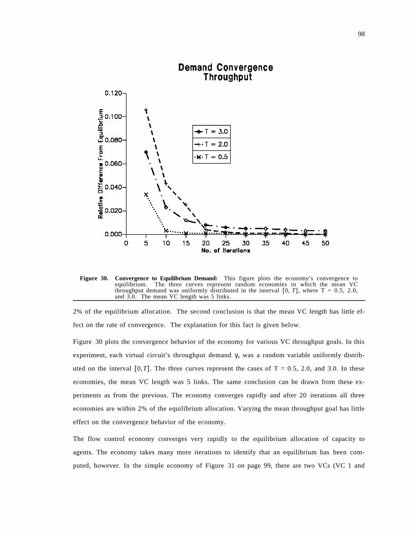
98

Figure 30. Convergence to Equilibrium Demand: This figure plots the economy′s convergence toequilibrium. The three curves represent random economies in which the mean VCthroughput demand was uniformly distributed in the interval [0, T ], where T = 0.5, 2.0,and 3.0. The mean VC length was 5 links.

2% of the equilibrium allocation. The second conclusion is that the mean VC length has little ef-

fect on the rate of convergence. The explanation for this fact is given below.

Figure 30 plots the convergence behavior of the economy for various VC throughput goals. In this

experiment, each virtual circuit′s throughput demand γa was a random variable uniformly distrib-

uted on the interval [0,T ]. The three curves represent the cases of T = 0.5, 2.0, and 3.0. In these

economies, the mean VC length was 5 links. The same conclusion can be drawn from these ex-

periments as from the previous. The economy converges rapidly and after 20 iterations all three

economies are within 2% of the equilibrium allocation. Varying the mean throughput goal has little

effect on the convergence behavior of the economy.

The flow control economy converges very rapidly to the equilibrium allocation of capacity to

agents. The economy takes many more iterations to identify that an equilibrium has been com-

puted, however. In the simple economy of Figure 31 on page 99, there are two VCs (VC 1 and

99

Figure 31. Convergence detection problem.

VC 2). P1 = 1,3 and P2 = 2,3, and both VCs have W = 1 and γ = 1. The supply vector is

S•

= <1, 1, 1.98>. By symmetry and lemma 1.1, the equilibrium allocation for this economy is:

1. VC 1 gets <0.99, 0, 0.99>.

2. VC 2 gets <0, 0.99, 0.99>.

In the simulation of this simple economy, the minimum price was ε = 0.001. The economy required

over 1000 iterations to detect that it had computed an equilibrium. The economy did converge very

rapidly to the equilibrium, but did not realize that it had. After only four iterations,

d•

(p• 4) − d•

(p• *)

d•

(p• *)= 0.002.

100

The detection problem is caused by the fact that in equilibrium some resource may have demand

slightly less than supply. In this case, the price of the resource is slowly driven down to ε. Let i

be the most utilized link whose equilibrium demand is less than supply. That is, the i that mini-

mizes:

∆ =(Si − di(p

• *))Si

and has p*i = ε. Suppose that the equilibrium allocation for this link is computed in iteration L. The

economy must drive the price of edge i to ε. The price pKi in iteration K > L is simply

pLi • (1 − ∆)(K − L).

For pKi ≤ ε, we have

K = L +log ε − log pL

i

log(1 − ∆). (2)

As ∆ → 0, the value of K in equation (2) goes to infinity. Factors such as mean VC throughput

goal and mean VC length only indirectly effect the detection of equilibrium. The detection of

equilibrium is solely determined by the most utilized, non-saturated link.

There are heuristic solutions to the equilibrium detection problem. One approach is to arbitrarily

stop the economy after some threshold K iterations. Our experiments suggest that K = 25 yields

allocations within 2% of optimal for realistically large networks. Another approach is to monitor

the change in demand in successive iterations. In this case, the economy stops iterating if

d•

(p• k + 1) − d•

(p• k)

d•

(p• k)≤ δ,

where δ is a parameter. We implemented and tested this second heuristic for the economies of

Figure 29 on page 97, Figure 30 on page 98 and Figure 31 on page 99, setting δ = 0.01. The

heuristic detects equilibrium in the pathological economy of Figure 31 on page 99 after 2 iterations.

The relative error in the demand vector when the heuristic guesses that equilibrium was found was

0.002. For the six sets of random economies of Figure 29 on page 97 and Figure 30 on page 98,

101

on the average the heuristic guesses that equilibrium has been found after 10.1 iterations. The av-

erage relative error if the economy stopped when equilibrium was guessed was 0.021.

4.4.1 Network Updates

The simulation experiments in the preceding discussion demonstrated that the flow control econ-

omy can rapidly compute an equilibrium allocation of resources when starting from an initial state

in which no resources have been allocated. In this section, we study the convergence of the econ-

omy to a new equilibrium when a VC leaves the economy, or when a new VC is started up.

Figure 32 on page 102 contains the results of simulation experiments testing the convergence. In

this figure, a network with 25 links and 50 random VCs is generated and the equilibrium is com-

puted. Then a VC addition or deletion is simulated. After each change, the new equilibrium is

computed. The curves represent the average number of iterations required to reach the new equi-

librium. The three cases are: 1) Adding 50 VCs, 2) Deleting 50 VCs, and 3) a random ordering of

50 additions and deletions.

Three main conclusions can be drawn from these experiments. First, the economy rapidly computes

the new equilibrium after an update. The economy is within 5% of the new equilibrium after 15

iterations in all cases. The second conclusion is that moving from one equilibrium to the new

equilibrium after an update requires approximately as many iterations as the computation of the

initial equilibrium. This is due to the same phenomenon described above. The third conclusions

is that the flow control economy can effectively deal with dynamic network environments.

In the simulations in this section, the path chosen for a new VC is determined before the economy

starts iterating to a new equilibrium. The price information can help the VC agent choose the

″best″ path. However, the VC cannot change its routing decision after the tatonement process be-

gins. That is, dynamic routing after each price update cannot be allowed. If this is allowed, there

are cases in which an equilibrium will never be computed.

Figure 33 on page 103 depicts an example of this problem. In this figure, there are three links

e1, e2 and e3. Each link has Si = 1 and initial price pi = ε, and we assume ε < 0.5. There is a single

VC agent that wants to route traffic from node 1 to node 3. This agent has throughput goal

γ = ∞ and wealth W = $1. The agent can choose either path {e1, e2} or simply {e3}. The agent

choose the cheaper path {e3} and demands capacity 1ε which is greater than S3. So, p3 increases.

As soon as p3 > 2 • ε, the agent switches to the cheaper path {e1, e2} and demands capacity 12 • ε

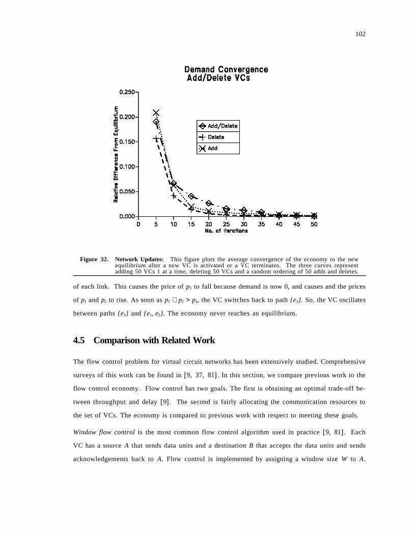
102

Figure 32. Network Updates: This figure plots the average convergence of the economy to the newequilibrium after a new VC is activated or a VC terminates. The three curves representadding 50 VCs 1 at a time, deleting 50 VCs and a random ordering of 50 adds and deletes.

of each link. This causes the price of p3 to fall because demand is now 0, and causes and the prices

of p1 and p2 to rise. As soon as p1 + p2 > p3, the VC switches back to path {e3}. So, the VC oscillates

between paths {e3} and {e1, e2}. The economy never reaches an equilibrium.

4.5 Comparison with Related Work

The flow control problem for virtual circuit networks has been extensively studied. Comprehensive

surveys of this work can be found in [9, 37, 81]. In this section, we compare previous work to the

flow control economy. Flow control has two goals. The first is obtaining an optimal trade-off be-

tween throughput and delay [9]. The second is fairly allocating the communication resources to

the set of VCs. The economy is compared to previous work with respect to meeting these goals.

Window flow control is the most common flow control algorithm used in practice [9, 81]. Each

VC has a source A that sends data units and a destination B that accepts the data units and sends

acknowledgements back to A. Flow control is implemented by assigning a window size W to A.

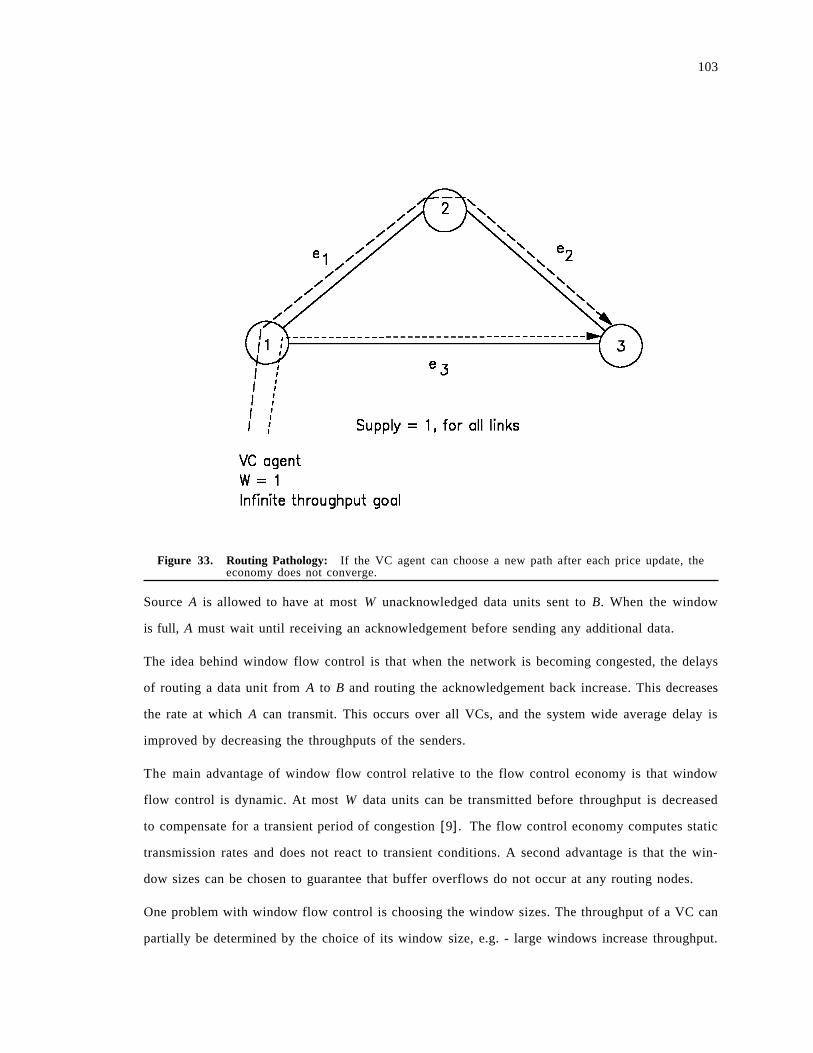
103

Figure 33. Routing Pathology: If the VC agent can choose a new path after each price update, theeconomy does not converge.

Source A is allowed to have at most W unacknowledged data units sent to B. When the window

is full, A must wait until receiving an acknowledgement before sending any additional data.

The idea behind window flow control is that when the network is becoming congested, the delays

of routing a data unit from A to B and routing the acknowledgement back increase. This decreases

the rate at which A can transmit. This occurs over all VCs, and the system wide average delay is

improved by decreasing the throughputs of the senders.

The main advantage of window flow control relative to the flow control economy is that window

flow control is dynamic. At most W data units can be transmitted before throughput is decreased

to compensate for a transient period of congestion [9]. The flow control economy computes static

transmission rates and does not react to transient conditions. A second advantage is that the win-

dow sizes can be chosen to guarantee that buffer overflows do not occur at any routing nodes.

One problem with window flow control is choosing the window sizes. The throughput of a VC can

partially be determined by the choice of its window size, e.g. - large windows increase throughput.

104

However, the throughput and delay of the VC are also determined by the window sizes of other

VCs. This makes the choice of window sizes complicated. The flow control economy has a similar

problem with the initial endowment of wealth to VCs. Exploring how the choice of the Wa′s effects

the relative throughputs and delays of the VCs is left for future work.

Another problem with window flow control is that it implements a system wide throughput-delay

trade-off. For example, the set of VCs experiencing delays due to congestion may be throughput

oriented, and should not have their window sizes decreased. The flow control economy does not

have this problem.

Window flow control can be unfair to short VCs [9]. The window size of a VC must be an in-

creasing function of the number of links in its path to meet its throughput goals during periods with

light contention. During periods of congestion, this makes it likely that a long VC gets more ca-

pacity of a heavily loaded link than a shorter VC sharing the same link [9]. The fairness of the flow

control economy with respect to long VCs versus short VCs was described in section 2.

The flow control problem can be combined with circuit routing to form a single optimization

problem [9]. The problem is to choose a path Pa and a transmission rate ra for each VC a that

minimizes:

∑a

Da + ∑a

ea(ra).

Da is VC a′s delay given the routing and transmission rates. ea(ra) is a penalty function for the VC.

As ra decreases, this function increases and defines the penalty for flow controlling this circuit.

The main disadvantage to this approach is the it requires computationally intensive, centralized

computing to determine the routing and transmission rates. The flow control economy also per-

forms a minimization problem when the VCs try to minimize delay. We have a efficient algorithm

that is specific to our optimization problem. It is not clear how the computational overheads of

the two approaches compare.

A second disadvantage of the combined routing-flow control problem is that the optimization must

be recomputed each time a new VC is activated or an existing VC terminates. This incurs overhead.

Furthermore, the new paths may be different from the existing paths. So, additional overhead is

incurred terminating the existing paths and starting the new ones.

105

The definition of the penalty functions adds complexity to the flow control problem. ea must reflect

VC a′s need for throughput. The rate actually assigned to VC a also depends on the penalty func-

tions of other VCs. So, the interactions between the penalty functions increase problem complexity.

The assignment of wealth to a VC in the flow control economy also should consider the values

assigned to other VCs. This is straight forward, however, and does not require comparisons of

throughput-delay goals.

Finally, combining routing and flow control in a single optimization problem may assign 0

throughput to some VCs. So, it is not fair be condition F1.

The main advantage of the combined flow control-routing approach is that it can improve on the

allocations given to the VCs compared to the flow control economy. We have proven that the

economy computes pareto-optimal resource allocations given a fixed set of VC paths. However,

choosing an alternate set of paths may result in an allocation the improves the lot of all VCs. We

demonstrated that the economy cannot implement dynamic routing in addition to flow control.

This is a major shortcoming of the economy. Quantifying the performance degradation due to not

dynamically assigning routes is an area for future work.

A third class of flow control algorithms are Bottleneck or max-min algorithms [9]. These algo-

rithms are based input rate adjustment. The algorithms′ primary goals is to compute allocations

which are fair by condition F2. An efficient decentralized algorithm for computing rate assignments

that are fair by condition F2 has been proposed by Jaffe [48]. Other algorithms are presented in

[9].

The main disadvantage of bottleneck flow control is the assumption that all VCs are throughput

oriented. This approach is less general than the flow control economy. We compared the fairness

properties of the economy with bottleneck flow control in section 1.

A major benefit of the flow control economy is that it supports decentralized choice of individual

throughput-delay trade-offs. Some previous work on the flow control problem has allowed a VC

to define its throughput-delay goals independently of other VCs. Sanders [78, 79] presented an

algorithm for computing optimal transmission rate allocations under a model in which each VC

has an individual utility function that defines its throughput-delay trade-off. Possible utility functions

were not defined. Sanders algorithm is decentralized and asynchronous, and maximizes the sum

of the individual utilities. The algorithm can assign transmission rate 0 to a circuit and is unfair by

condition F1. The algorithm also requires some coordination between choice of utility functions.

106

Bharath-Kumar and Jaffe [10] proposed a generalized form of power for for representing

throughput-delay trade-offs. This work focused on maximizing a global objective function based

on the power obtained by individual VCs, e.g. - the sum of the individual powers. The individual

VCs did not choose their own definition of power and were assumed to be homogeneous, however.

In some examples, their algorithm computes rate allocations that are a Nash Equilibrium. It was

shown in section 2 that a Nash Equilibrium is not Pareto-optimal. In their work, Bharath-Kumar

and Jaffe observed that their algorithm computed an allocation that could be improved upon by

all VCs.

The related flow control work described in chapter 2 and that of Bharath-Kumar and Jaffe use

power to model throughput-delay trade offs. Let γk be VC k′s throughput, and Dk is its delay. VC

k chooses a constant βk and attempts to maximize its power

(γk)βk

Dk.

Power is an awkward representation for a individual VC throughput-delay goals. It would be very

difficult for the user of VC k to choose the constant βk that achieves its throughput-delay goals.

The model used in the flow control economy makes specifying throughput-delay goals simpler.

4.6 Conclusions

In this chapter we have applied concepts from mathematical economics to develop an effective flow

control mechanism. The immediate advantages of our algorithm compared to previous flow control

mechanisms, are that: 1) it captures in a precise manner both diversity of priorities among virtual

circuits in a network as well as diversity of their performance objectives (throughput vs. delay). 2)

it accomplishes resource allocations that are optimally fair (in a formal sense).

Our algorithm is decentralized and is simple to implement. Additionally, simulation studies dem-

onstrated that the economy efficiently computes optimal resource allocations for realistically large

networks. We showed that the economy rapidly computes the new optimal allocation when a new

virtual circuit is activated or an existing circuit terminates. Finally, we demonstrated the limitations

of the economy as a dynamic, virtual circuit routing algorithm through a simple example.

In this chapter, we demonstrated the benefits of applying economic theory to resource management

problems in distributed systems. Pareto-optimality was shown to provide a powerful new definition

107

for optimal, fair resource allocations in heterogeneous network environments. Economic techniques

were used to prove optimality of the competitive equilibrium computed by the economy, and that

an equilibrium does exist for all networks under our model. This chapter illustrated that two main

challenges must be overcome when applying economic theory to resource management in distrib-

uted computer systems. First, the underlying economic models must be modified to accurately re-

flect the problem being studied. Secondly, and most importantly, it must proven that the system

possesses fundamental properties assumed by economic theory, and it cannot be assumed that the

economy possesses these properties. For example, continuity of demand with respect to prices is

assumed in economic theory. In this chapter we had to prove that the agents′ diverse demand

functions were continuous.

Several areas for future work remain. First, two theoretical questions were raised. One is uniqueness

of the equilibrium allocation. The second is a proof of convergence or a counter example. Another

area is expanding the economy to incorporate other models of VC goals. This would increase the

generality of the results. Finally, the use of link prices to determine long term routing decisions,

to guide capacity planning and to set demand based rate setting in public access networks are po-

tentially fruitful areas for further work.

4.7 Proof of Lemmas

This section proves lemmas on which results in this chapter depend. Let G = < V , E> be the

graph of the underlying network, and let the current price vector be p• = < p1, p2, ... , pm> with

0 < ε ≤ pi < ∞ for all i. A VC agent a in this economy has a non-empty path

Pa = {la,1, la,2, ... , la,m(a)}, wealth Wa > 0 with which it purchases allocations and a throughput goal

γa. To make the notation simpler, the p•

will be dropped from the allocation vectors when the

context is clear, i.e. - φ•

(p• ) is written simply φ•

.

For the proof of lemma 1.1, define a special allocation β•

a for VC a with:

1. βai = 0, if i∉Pa.

2. βai =

Wa

Qa, if i ∈ Pa.

where Qa = ∑i ∈ Pa

pi.

Lemma 1.1 : If Wa ≤ Qa • γa at prices p•

, then:

108

1. Φa(p• ) is non-empty.

2. Φa(p• ) has a single element φ

•.

3. φ i =Wa

Qa, if i ∈ Pa.

4. φ i = 0, if i∉Pa.

Proof:

All four propositions will be proven if we can show β•

a is VC a′s unique optimal choice at prices

p•

.

First,

β• a = ∑

i ∈ Pa

pi •Wa

Qa=

Wa

Qa• Qa = Wa.

So β•

a is affordable and Ba(p• ) is not empty. The preference relation • a is a partial order, and has a

maximal element. This means that Φa(p• ) is not empty.

Suppose there exists another allocation α• a • β•

a. Then we have the following:

1. αai ≥ 0 implies that αa

i ≥ βai for i∉Pa.

2. T(α• a) ≥ T(β•

a), which in turn implies αai ≥

Wa

Qa, i ∈ Pa.

If α• a ∼ a βa•

, then T(α• a) = T(α• a) =Wa

Qa and α• a = β

•a. If αa

•• a βa

•, then T(α• a) > T(α• a) =

Wa

Qa. This

means αai >

Wa

Qa, and α• a • p

• > Wa. So, α• a is not affordable.

Lemma 2.1 : Let (1) p•

be a price system. (2) φ•

a(p• ) be agent a′s demand at p•

. (3) x• ≠ φ

•a(p• ) be any

allocation. Then,

1. φ•

a(p• ) • p• = Wa.

2. x• • a φ

•a(p• ) implies that x

•• p

• ≥ φ•

a(p• ) • p•

.

3. x• • a φ

•a(p• ) implies x

•• p

• > φ•

a(p• ) • p•

.

Proof:

109

If T(φ•

a(p• )) ≤ γa the results are obvious. So, assume that T(φ•

a(p• )) ≥ γa.

(1) If φ•

a(p• ) • p• < Wa, then VC a has a surplus of δ = Wa − φ

•a(p• ) • p

•, with δ > 0. Buying δ

piof any

link i ∈ Pa improves the delay because delay decreases monotonically as a function of xi when

xi ≥ γ a. So, φ•

a(p• ) was not optimal, and this is a contradiction.

(2,3) Assume the opposite: x• • a φ

•a(p• ), and x

•• p

• < φ•

a(p• ) • p•

. Perform the following transforma-

tions

1. ui = φ ai (p

• ) − γa, for i ∈ Pa.

2. wi = xi − γ a, for i ∈ Pa.

3. ui = φ ai (p

• ), i∉Pa.

4. wi = xi, i∉Pa.

This means that p•

• w• ≤ Wa − Qa × γa, and w

• is feasible (affordable). x

• ∼ a φ•

a(p• ) means that in the

minimization problem of section 2, F(u• ) = F(w• ). This contradicts the strong convexity of F. If

x• • a φ

•a(p• ), then F(w• ) < F(u• ). This contradicts the optimality of u

• and the definition of φ

•a(p• ).

lemma 3.1 : F(u• ) is continuous and strongly convex.

Proof: :

F is the sum of m functions

Fi(u• ) = 1

Ki + ui

each of which is strongly convex and continuous (Ki > 0, ui ≥ 0). Figure 34 on page 110 shows the

form of Fi. It is clear that the segment connecting Fi(w) and Fi(v) always lies above the curve.

Strong convexity of the Fi′s means that for all u, w ∈ U,

α • Fi(u• ) + (1 − α) • Fi(w

• ) > F(α • u• + (1 − α) • w

• ).

This in turn implies,

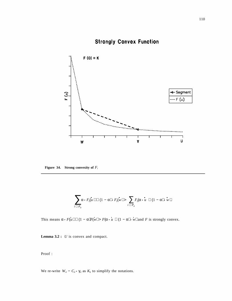
110

Figure 34. Strong convexity of Fi

∑i ∈ Pa

α • Fi(u• ) + (1 − α) • Fi(w

• ) > ∑i ∈ Pa

Fi(α • u• + (1 − α) • w

• ).

This means α • F(u• ) + (1 − α)F(w• ) > F(α • u• + (1 − α) • w

• ) and F is strongly convex.

Lemma 3.2 : U is convex and compact.

Proof :

We re-write Wa − Ca • γa as Ka to simplify the notations.

111

(Compact) : U is compact if it is bounded and closed. By definition, U is bounded below by

0•

= <0, 0, ..., ... , 0>. We know that p•

• u• ≤ Ka. This requires that pi • ui ≤ Ka which in turn means

that ui ≤Ka

pi. We know that pi > 0 which means that

Ka

pi< ∞ . So, U is bounded from above by

the vector

<Kap1

,Kap2

, ... ,KapM

> .

For U to be closed, any sequence of vectors u• n ∈ U that converges must converge to an element u

• *

of U. Assume the sequence u• n, n = 1, 2, ... converges to u

• *. This means that for all i = 1, 2, ... , M,

uni converges to u*

i . Assume that u*i < 0. This means that u*

i = 0 − δ, δ > 0. By definition, uni ≥ 0, for

all n. This means that lim uni − u*

i ≥ δ. This contradicts the assumption of convergence, and

u*i ≥ 0, i = 1, 2, ... , M.

p•

• u• n − p

•• u

• * =

∑M

i = 1

uni − u*

i • pi.

We know that as n → ∞ , uni − u*

i → 0 that in turn implies p•

• u• n − p

•• u

• * → 0. We know that

p•

• u• n ≤ Ka, so p

•• u

• * ≤ Ka.

We have shown that u*i ≥ 0 and p • u

• * ≤ Ka. So, u• * ∈ U and U is closed. U is closed and bounded

which means that it is compact.

(Convex) : For U to be convex, for any two vectors u, v ∈ U and any α, 0 ≤ α ≤ 1, the vector

w• = α • u

• + (1 − α)v•

must be in U. By definition, ui ≥ 0, vi ≥ 0, α ≥ 0 and 1 − α ≥ 0, so wi = α • ui + (1 − α) • wi ≥ 0.

p•

• w• = p

•• (α • u

• ) + p•

• ((1 − α) • v• ). This in turn means, p

•• w

• = α • (p• • u• ) + (1 − α) • (p• • v

• ). By

definition, p•

• u• ≤ Ka and p

•• v

• ≤ Ka. So, p•

• w• ≤ α • Ka + (1 − α) • Ka = Ka.

Lemma 3.3 : : A sequence of points {x•

m} in • N converges to x• 0 if, and only if, every sub sequence

{x• mk} contains a subsequence {x

• m′k} that converges to x• 0.

112

Proof :

The if part follows directly from the definition of convergence

For the only if part, assume that x• m→/ x

• 0. Also assume that every subsequence contains a subse-

quence converging to x• 0.

x• →/ x

• 0 implies that there exists a ε > 0 such that for any k ≥ 1, there is an mk such that

x• mk − x

• 0 > ε. For k = 1, 2, ... take the sequence of points x• mk. By definition, this sequence

cannot contain a subsequence converging to x• 0 because for all k, x

• mk − x• 0 > ε.

This contradicts the assumptions, and the lemma is shown.

We now prove one of the assertions made in the proof of continuity of a VC′s demand function

with respect to prices. This was theorem 4.2. Let x• 0, p

• 0, p• m be defined as for theorem 4.2. For the

sequence of points p• m → p

• 0, define a sequence of points w• m ∈ U(p• m) where

x• 0 − w

• m ≤ x• 0 − z

• m

for all z• ∈ U(p• m). We prove the following lemma:

Lemma 3.4 : As p• m → p

• 0, x• 0 − w

• m → 0.

Proof :

We construct a sequence y• m that converges to x

• 0. This will prove convergence of w• m.

If x• 0 = 0

•then y

• m = 0•

.

Assume that x• 0 is a vector in U(p• 0). Let S⊆{1, 2, ... , M} be the links for which x

• 0i > 0. Define em

as

em = min {(p0s − pm

s ) s ∈ S}.

We have em → 0.

We know that

pms + em ≤ p0

s . (1)

The budget constraint tells us that

113

∑M

i = 1

p0i x 0

i ≤ W − γ∑M

i = 1

pi.

Plugging the inequality (1) into the budget constraint gives

∑s ∈ S

(pms + em)x 0

s ≤ W − γ(∑N

i = 1

pmi ) − γemM.

Rearranging terms gives

∑s ∈ S

pms x 0

s + em∑s ∈ S

x 0s + γemM ≤ W − γ∑

M

i = 1

pmi .

We multiply and divide the second term in this inequality by the cardinality of S, denoted S , and

get

∑s ∈ S

pms x 0

s + S em((∑s ∈ S

x 0s)+ γM

S )≤ W − γ∑M

i = 1

pmi . (2)

For simplicity of notation, let

A =(∑

s ∈ S

x 0s)+ γM

S.

By definition of the cardinality of a set we have

114

S eM A = ∑s ∈ S

eM A,

and multiplying and dividing each i-th term pmi gives

S eM A = ∑s ∈ S

pms (eM A

pms

).

This means we can rewrite inequality (2) as

∑s ∈ S

pms (x 0

s +emA

pms)≤ W − γ∑

M

i = 1

pmi . (3)

We know that em → 0, and pms → p0

s . By definition, p0s > 0, and by the definition of the set S, we

know x 0s > 0. This implies that we can find K ∈ • such that for all s ∈ S, if m > K,

x 0s ≥ −

em

pms

•A

S . (4)

The sequence {y• m} is defined by components as follows:

1. ymi = 0, if m ≤ K

2.

y mi = x 0

i +em

pms

•A

S , if m > K and i ∈ S

3. ymi = 0, if m > K and i∉S

From inequality (4), we know that ymi ≥ 0, and inequality (3) shows that y

• m is affordable. So,

y• m ∈ U(p• m).

We know that:

1. em → 0.

115

2. pmi → p0

i > 0.

3. S > 0.

This means that ymi → x m

i . This proves the lemma

116

5.0 The Data Management Economy

This chapter presents an economy that manages data objects in a distributed system. The econo-

my′s goal is to improve performance by regulating the number of copies of each object, and the

assignment of copies to processors. The effectiveness of the economy is evaluated by a simulation

based performance study.

The main results of this section is a set of simulation based performance experiments that demon-

strates that the data management economy substantially improves performance compared to static

global policies. The improvement is achieved in two ways. First, the number of copies of each

data object is controlled to reflect the ratio of read access vs. write access. When an object is written,

all copies must be updated. If the write access rate is high, there should be few copies to avoid

update overhead. If read access is predominant, there should be many copies. This increases the

probability that a read can be processed locally or at a nearby processor. The second way in which

performance is improved is by assigning the copies to processors based on localities in transaction

reference patterns. This increases the probability of a data access be satisfied locally or at a nearby

processor. Both of these improvements are achieved by decentralized, competitive decision making.

This chapter is structured as follows. Section 1 describes the distributed system and defines the data

management problem. Section 2 presents the data management economy and a running example.

The main results of this chapter are contained in performance experiments described in section 3.

The data management economy solves a general version of the File Allocation Problem. Previous

work on this problem is compared with the economy in section 4. Section 5 contains conclusions

and directions for future work.

5.1 Problem Statement and System Model

The distributed system consists of N processing nodes P1, P2, ... , PN. Each Pi has a processing pa-

rameter ri that defines the rate at which it can process operations on local data. The nodes are

connected by a set of communication links E = {e• }, and link e• has delay d• .

There are M data objects in the system denoted D1, D2, ... , DM. S(Di) defines the size of Di in bytes.

The problem definition treats the data objects as abstract resources. In a real system, they could

correspond to Relations [20, 21], tuples, files, records or any other data structure. There may be

multiple copies of each data object at distinct processor nodes.

117

Transactions enter the system at all processors. A transaction is a sequence of Read and Write op-

erations on the data objects. We assume that a transaction′s operations must be serviced sequen-

tially. Operation Read(Di) can be performed on any copy of Di. If a transaction submits

Write(Di, value), all copies are updated.

The data management problem is to minimize mean transaction response time. The parameters that

can be controlled are: 1) The number of copies of each data object. 2) The assignment of copies

to processing nodes.

Our model does not explicitly study the effects of concurrency control [8]. The data management

economy is compatible with concurrency control protocols that do block transactions, e.g. -

Timestamp, Optimistic [7, 8]. Expanding the model to include lock based concurrency control is

an area for future work.

5.2 The Economy

There are four types of agents in the data management economy. These are transactions,

processors, data object managers and local data agents. A transaction T that enters the system at

node Pi pays Pi to perform its data access operations. T is endowed with an initial allocation of

money MT.

Processor node Pi sells data access to local transactions. To do so, Pi leases copies of data objects

from the data object managers. If transaction T submits a Read(Dj) or a Write(Dj, value) and Pi

does not lease a copy of object Dj, the work is subcontracted to some processor with a copy. A

processor′s sole goal is to maximize profit.

Each data object is controlled by a data object manager that leases copies of the object to

processors. The data object manager for Dj is also responsible for updating all copies when a

Write(Dj, value) occurs. A data object manager′s goal is to maximize profit.

There is one local data agent at each node in the system. The local data agent at Pi acts as an in-

termediary between Pi and the object managers, which may reside at other nodes. Figure 35 on

page 119 shows a simple data management economy that is used as an example in this chapter.

There are three processors in this economy (P1, P2, P3) and three objects (A, B, C). There may be

multiple read copies of an object, but only one write copy exists. In the example, P1 has a read

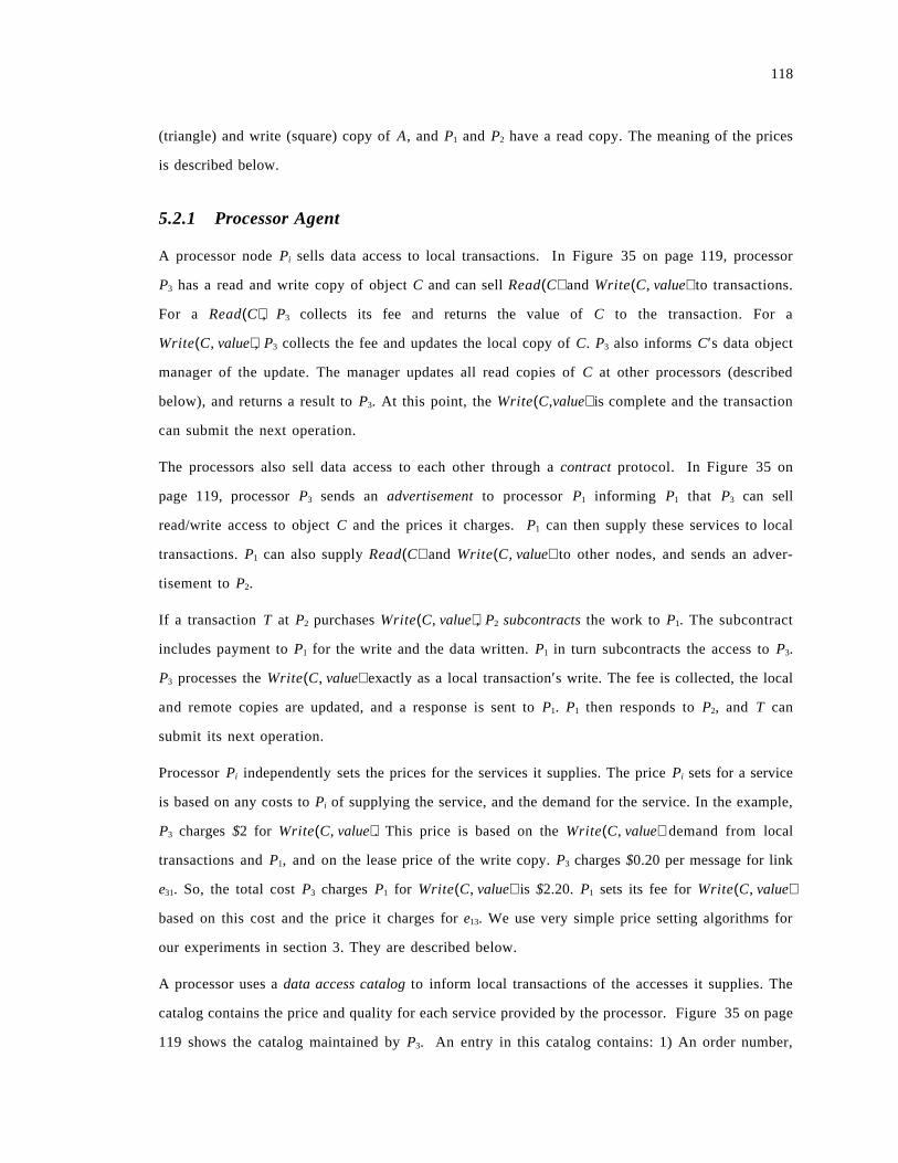
118

(triangle) and write (square) copy of A, and P1 and P2 have a read copy. The meaning of the prices

is described below.

5.2.1 Processor Agent

A processor node Pi sells data access to local transactions. In Figure 35 on page 119, processor

P3 has a read and write copy of object C and can sell Read(C) and Write(C, value) to transactions.

For a Read(C), P3 collects its fee and returns the value of C to the transaction. For a

Write(C, value), P3 collects the fee and updates the local copy of C. P3 also informs C′s data object

manager of the update. The manager updates all read copies of C at other processors (described

below), and returns a result to P3. At this point, the Write(C,value) is complete and the transaction

can submit the next operation.

The processors also sell data access to each other through a contract protocol. In Figure 35 on

page 119, processor P3 sends an advertisement to processor P1 informing P1 that P3 can sell

read/write access to object C and the prices it charges. P1 can then supply these services to local

transactions. P1 can also supply Read(C) and Write(C, value) to other nodes, and sends an adver-

tisement to P2.

If a transaction T at P2 purchases Write(C, value), P2 subcontracts the work to P1. The subcontract

includes payment to P1 for the write and the data written. P1 in turn subcontracts the access to P3.

P3 processes the Write(C, value) exactly as a local transaction′s write. The fee is collected, the local

and remote copies are updated, and a response is sent to P1. P1 then responds to P2, and T can

submit its next operation.

Processor Pi independently sets the prices for the services it supplies. The price Pi sets for a service

is based on any costs to Pi of supplying the service, and the demand for the service. In the example,

P3 charges $2 for Write(C, value). This price is based on the Write(C, value) demand from local

transactions and P1, and on the lease price of the write copy. P3 charges $0.20 per message for link

e31. So, the total cost P3 charges P1 for Write(C, value) is $2.20. P1 sets its fee for Write(C, value)

based on this cost and the price it charges for e13. We use very simple price setting algorithms for

our experiments in section 3. They are described below.

A processor uses a data access catalog to inform local transactions of the accesses it supplies. The

catalog contains the price and quality for each service provided by the processor. Figure 35 on page

119 shows the catalog maintained by P3. An entry in this catalog contains: 1) An order number,

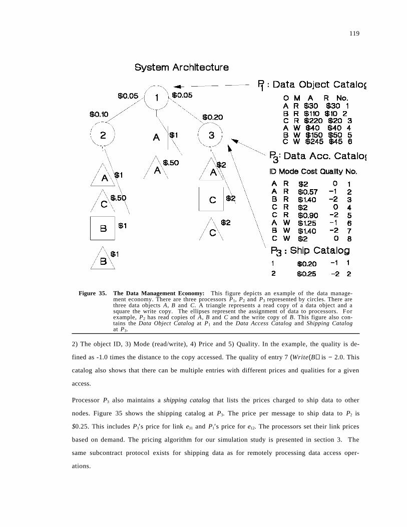
119

Figure 35. The Data Management Economy: This figure depicts an example of the data manage-ment economy. There are three processors P1, P2 and P3 represented by circles. There arethree data objects A, B and C. A triangle represents a read copy of a data object and asquare the write copy. The ellipses represent the assignment of data to processors. Forexample, P2 has read copies of A, B and C and the write copy of B. This figure also con-tains the Data Object Catalog at P1 and the Data Access Catalog and Shipping Catalogat P3.

2) The object ID, 3) Mode (read/write), 4) Price and 5) Quality. In the example, the quality is de-

fined as -1.0 times the distance to the copy accessed. The quality of entry 7 (Write(B)) is − 2.0. This

catalog also shows that there can be multiple entries with different prices and qualities for a given

access.

Processor P3 also maintains a shipping catalog that lists the prices charged to ship data to other

nodes. Figure 35 shows the shipping catalog at P3. The price per message to ship data to P2 is

$0.25. This includes P3′s price for link e31 and P1′s price for e12. The processors set their link prices

based on demand. The pricing algorithm for our simulation study is presented in section 3. The

same subcontract protocol exists for shipping data as for remotely processing data access oper-

ations.

120

A processor leases a copy of a data object only if it is profitable to do so. To make leasing business

decisions, a processor records all data accesses it sells and all subcontracts it processes. In the ex-

ample, P1 records all of its sales of read and write access on object A. It also records all of the

Read(C) and Write(C, value) subcontracts it sends to P3, and all of the Read(B) and

Write(B, value) subcontracts it sends to P2. Processor P1 measures its average revenue for read and

write access to A and maintains its leases on these objects only if they are good investments. There

is a system wide interest rate I that formalizes the definition of a good investment. If L RA is the read

lease price of A, and RA is the average Read(A) revenue per lease period, P1 retains its read lease

on A only if

RA − L RA ≥ I • L R

A .

RA − L RA is P1′s profit on Read(A) per lease period. I • L R

A is the return on an investment of L RA

dollars if the money were deposited in a ″savings″ account.

A processor acquires a new lease if it estimates doing so will be a good investment. Assume that

P1 pays P2 and average of RB dollars per lease period for subcontracting Read(B). Two lease prices

are associated with a read copy of B : 1) The acquisition price L AB , and 2) The renewal price L R

B . If

P1 acquires a read lease, it pays L AB for the first lease period, and L R

B for subsequent renewals. (How

these prices are set and distributed is described below).

P1 acquires a read copy of B if

RB − L RB ≥ I • R A

B .

RB − L RB is the expected profit per lease period, and R A

B is the initial investment needed to make this

profit.

5.2.2 Data Object Agents

There are two types of agents associated with data objects. Each object A is controlled by a man-

ager MA, which resides with the write copy. The second type of agents are local agents. There is a

local agent at each processor Pi and this agent acts as a representative to Pi for the data object

managers located at other processors. In the example, MC is located at P3 and it uses the local agents

at P1 and P2 to interact with these processors.

121

The data object manager is responsible for updating the read copies of the object. Assume that P3

services a Write(C, value). P3 passes the update to MC. The agent MC sends the update to the local

agent at P2. MC uses the shipping catalog and must pay P3 $0.25 to send the data to P2. When the

update arrives at P2, the local agent submits the update operation at P2. Since this update does not

effect any other copies, the price charged by P2 is the local read price for C. This is $0.50 in the

example. After the update completes, the local agent at P2 sends a response and a bill to MC. When

this message arrives, MC informs P3 that the update is complete and then sends a check for $0.50

to the local agent at P2.

The data object manager sets the lease renewal and acquisition prices for the object. The goal is to

set the prices that maximize the object′s profit. The renewal price for the read copy is set based

on the demand for read copies. Many price functions are possible, and we propose a simple algo-

rithm in section 3. The read acquisition price is simply the renewal price plus the cost of shipping

a copy to the processor. In the example, the read renewal price of C is $20 and all objects require

1000 messages to ship a copy. So, the read acquisition price at P1 is $220.

Since there is only one write copy, the data object manager uses an auction to set the write renewal

price. The write renewal price has a lower bound which must cover the cost of updating the read

copies. This lower bound is determined by averaging the update cost per copy over time. Any bid

below this value is rejected.

The data object manager broadcasts all changes in renewal and acquisition prices to the local agents.

Each local agent posts these prices in a data object catalog. Figure 35 on page 119 contains the data

object catalog at P1. An entry in this catalog has the following fields: 1) The object ID, 2) The mode

(R/W), 3) The acquisition price, 4) The renewal price and 5) An order number.

A processor Pi uses the local data object catalog to determine renewal and acquisition prices. To

order an object, Pi sends a request to the local agent and pays the fee listed in the catalog. This re-

quest and the fee are forwarded to the data object manager. When receiving a lease request, the

manager pays the local processor Pj to ship a copy of itself to the processor ordering the copy.

When the copy arrives, Pi can start using it to supply service to transactions and other processors.

The local agent at Pi also collects and forwards renewal fees when Pi renews a lease, and informs

the manager when a lease is not renewed.

122

5.2.3 Transactions

A transaction T enters the system with an initial endowment of money MT and sequentially submits

read and write operations. T uses the data access catalog to order these services from the local

processor. In the example, if T arrives at P3 and wants to issue Read(A), T can either order catalog

entry 1 or entry 2. The decision is based on the amount of money the transaction possesses. In our

model, the transaction purchases the best service that it can afford. If T cannot afford any service,

for example it has only $0.50 remaining, it aborts. Other policies such as queueing are possible and

are left for future work.

5.3 Performance Evaluation

We implemented and simulated the data management economy to measure its performance. The

data management problem studied in this chapter is not mathematically tractable without relying

on simplistic analytical models of the underlying distributed system.

The economy was simulated on the 5 processor distributed system depicted in Figure 36 on page

123. There were 10 data objects, and each object contained 1000 records. Individual records were

the granularity of transaction access. The processor service time for an access on local data was 1

time unit. The processors serviced the local data accesses sequentially. The transmission delay per

message was 2 time units for all links. Each access request required 1 message, and shipping an

entire data object required 1000 messages.

The processors′ pricing policy for local resources was static with the following prices:

1. Read access : $0.50

2. Write access : $0.50

3. Link use : $0.01 per message

Each processor Pi marked up all of its costs by 10%. In the example, P3 charges P1 $2.20 for

Write(C, value). P1 would charge local transactions $2.47 = (1.1)($2.20) + $0.05 for Write(C, value).

In the simulations, a transaction T entered the system with MT = $10 and randomly submitted be-

tween 1 and 10 access operations. No transactions aborted due to insufficient funds. Applying

simple algebra to to Figure 36 on page 123 shows that the maximum cost for 10 data accesses is

less than $10.

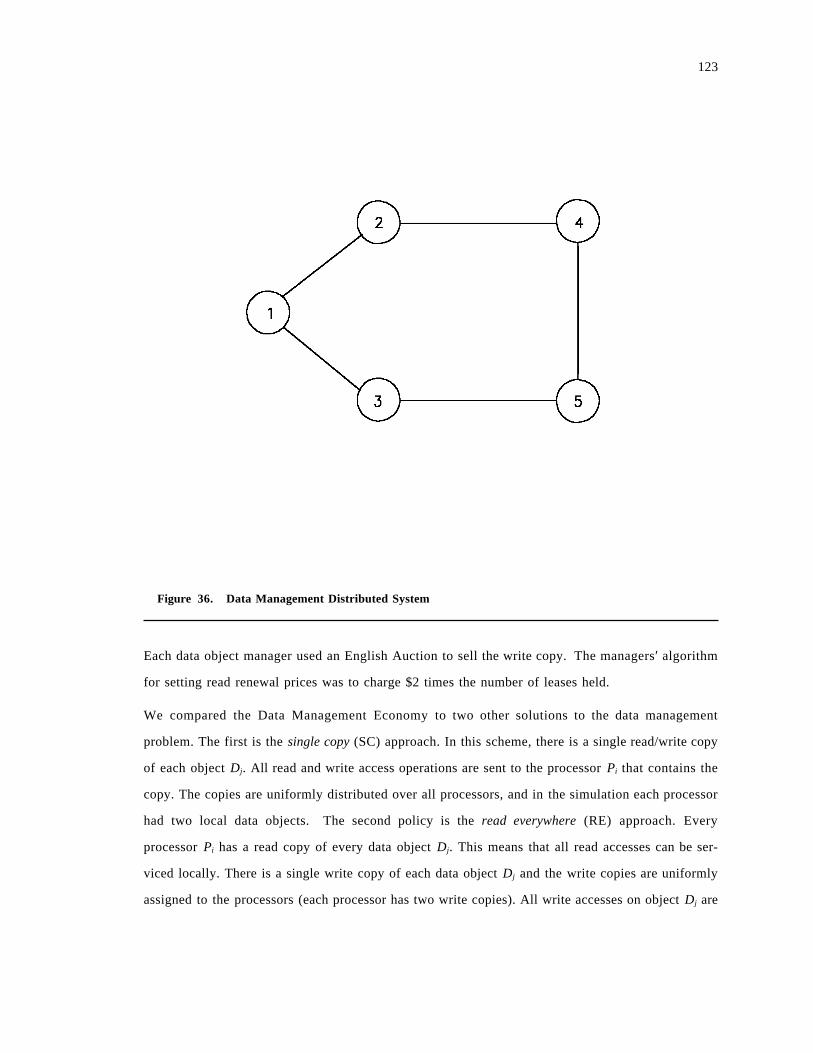
123

Figure 36. Data Management Distributed System

Each data object manager used an English Auction to sell the write copy. The managers′ algorithm

for setting read renewal prices was to charge $2 times the number of leases held.

We compared the Data Management Economy to two other solutions to the data management

problem. The first is the single copy (SC) approach. In this scheme, there is a single read/write copy

of each object Dj. All read and write access operations are sent to the processor Pi that contains the

copy. The copies are uniformly distributed over all processors, and in the simulation each processor

had two local data objects. The second policy is the read everywhere (RE) approach. Every

processor Pi has a read copy of every data object Dj. This means that all read accesses can be ser-

viced locally. There is a single write copy of each data object Dj and the write copies are uniformly

assigned to the processors (each processor has two write copies). All write accesses on object Dj are

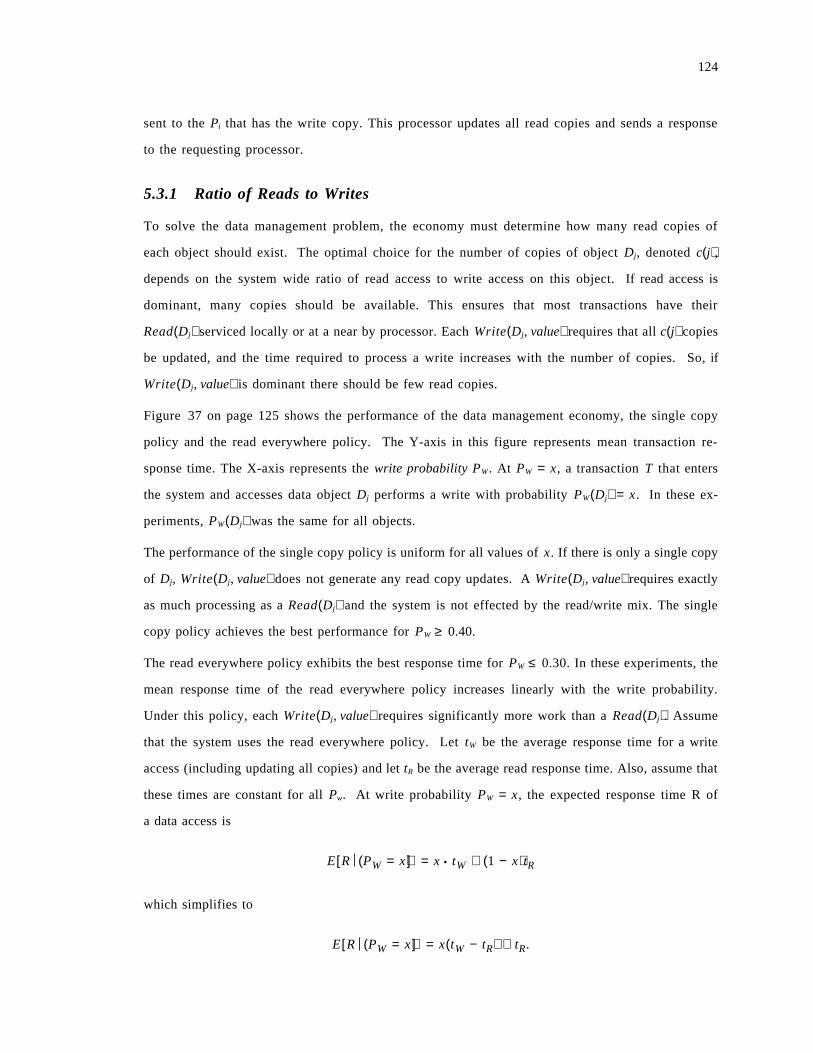
124

sent to the Pi that has the write copy. This processor updates all read copies and sends a response

to the requesting processor.

5.3.1 Ratio of Reads to Writes

To solve the data management problem, the economy must determine how many read copies of

each object should exist. The optimal choice for the number of copies of object Dj, denoted c(j),

depends on the system wide ratio of read access to write access on this object. If read access is

dominant, many copies should be available. This ensures that most transactions have their

Read(Dj) serviced locally or at a near by processor. Each Write(Dj, value) requires that all c(j) copies

be updated, and the time required to process a write increases with the number of copies. So, if

Write(Dj, value) is dominant there should be few read copies.

Figure 37 on page 125 shows the performance of the data management economy, the single copy

policy and the read everywhere policy. The Y-axis in this figure represents mean transaction re-

sponse time. The X-axis represents the write probability PW. At PW = x, a transaction T that enters

the system and accesses data object Dj performs a write with probability PW(Dj) = x. In these ex-

periments, PW(Dj) was the same for all objects.

The performance of the single copy policy is uniform for all values of x. If there is only a single copy

of Dj, Write(Dj, value) does not generate any read copy updates. A Write(Dj, value) requires exactly

as much processing as a Read(Dj) and the system is not effected by the read/write mix. The single

copy policy achieves the best performance for PW ≥ 0.40.

The read everywhere policy exhibits the best response time for PW ≤ 0.30. In these experiments, the

mean response time of the read everywhere policy increases linearly with the write probability.

Under this policy, each Write(Dj, value) requires significantly more work than a Read(Dj). Assume

that the system uses the read everywhere policy. Let tW be the average response time for a write

access (including updating all copies) and let tR be the average read response time. Also, assume that

these times are constant for all Pw. At write probability PW = x, the expected response time R of

a data access is

E[R (PW = x)] = x • tW + (1 − x)tR

which simplifies to

E[R (PW = x)] = x(tW − tR) + tR.

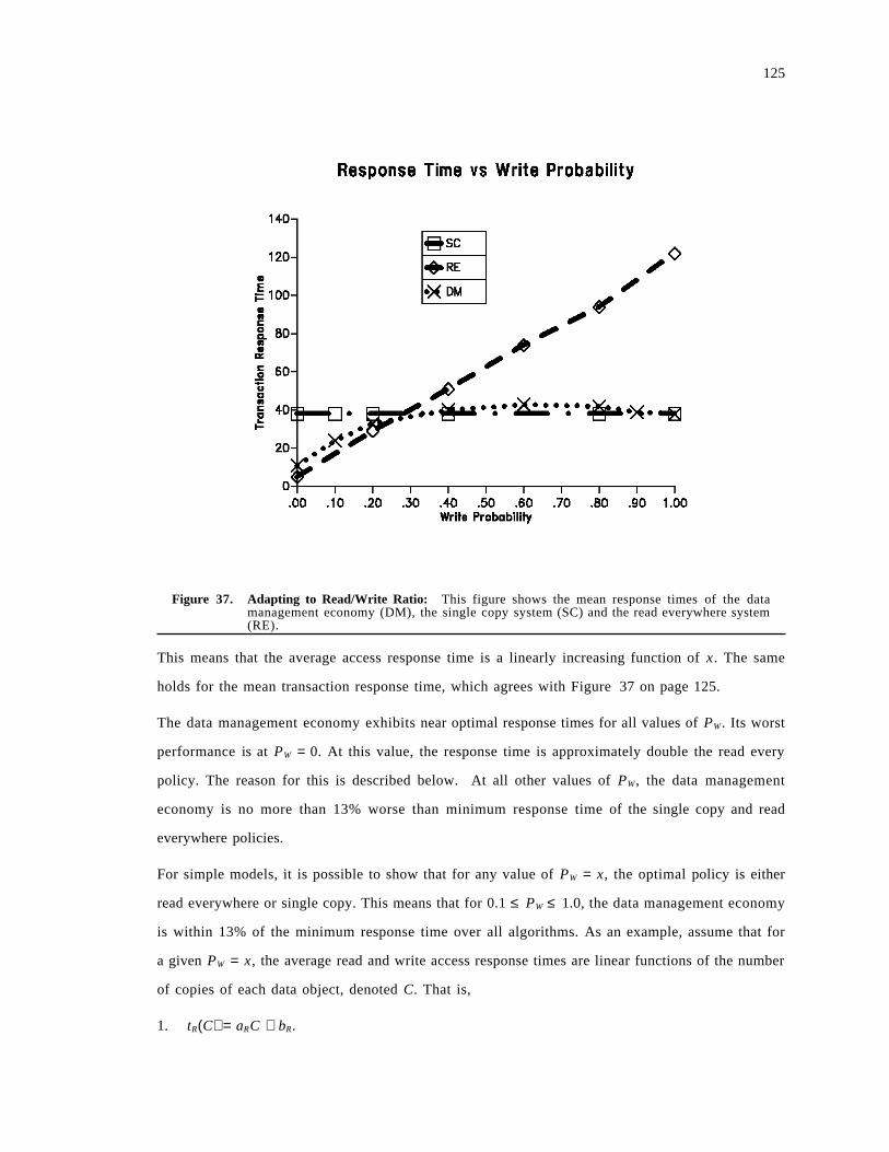
125

Figure 37. Adapting to Read/Write Ratio: This figure shows the mean response times of the datamanagement economy (DM), the single copy system (SC) and the read everywhere system(RE).

This means that the average access response time is a linearly increasing function of x. The same

holds for the mean transaction response time, which agrees with Figure 37 on page 125.

The data management economy exhibits near optimal response times for all values of PW. Its worst

performance is at PW = 0. At this value, the response time is approximately double the read every

policy. The reason for this is described below. At all other values of PW, the data management

economy is no more than 13% worse than minimum response time of the single copy and read

everywhere policies.

For simple models, it is possible to show that for any value of PW = x, the optimal policy is either

read everywhere or single copy. This means that for 0.1 ≤ PW ≤ 1.0, the data management economy

is within 13% of the minimum response time over all algorithms. As an example, assume that for

a given PW = x, the average read and write access response times are linear functions of the number

of copies of each data object, denoted C. That is,

1. tR(C) = aRC + bR.

126

2. tW(C) = aWC + bW .

The average response time at PW = x is

R(C) = (1 − x)tR(C) + xtW(C).

To find the optimal C, take the derivative of R(C). This is

R′(C) = (1 − x)aR + xaW .

The derivative is a constant, which means that R(C) takes its minimum value at either C = 0 or

C = N, where N is the number of processors. This analysis holds for all x, and under these simple

assumptions either the read everywhere or single copy policy is optimal for all x.

Two economic factors cause the data management economy to adapt the number of read copies

of each object Dj to the read/write ratio. These are:

1. The total revenue that all processors earn by selling Read(Dj) decreases as PW increases.

2. The read lease price for Dj increases linearly with the number of copies c(j).

For a given system wide arrival rate, this means that as PW increases, the processors as a whole can

afford fewer read copies.

Figure 38 on page 127 shows how the data management economy adapts the number of copies of

each object Dj to read/write ratio for it. In this example, there is a single data object A. The read

lease price is defined to be 5/3 times the number of leases held. Assume that on average, ten

transaction accessing A arrive at each processor during a lease period. Also assume that the

processors charge $0.50 for a Read(A). If PW = 0, each processor can earn $5 selling Read(A). The

system wide revenue is $15. The lease renewal price if three copies are leased is $53

× 3 = $5, and

3 copies can be afforded by the system as a whole. (To avoid complicating the example, the interest

rate I = 0). At PW = 0.50, half of the accesses are writes and only $7.50 worth of Read(A) business

enters the system per lease period. The total lease price for 3 leases is $15, and the total for two

leases is $6.67. This means that the system as a whole can only afford two copies. In the example

of Figure 38 on page 127, P1 subcontracts its Read(A) to P2 and P3. Finally, at PW = 0.80, the total

Read(A) revenue in the economy is $3 and only one copy is affordable. How the copies are as-

signed to the processors is described in a subsequent subsection.

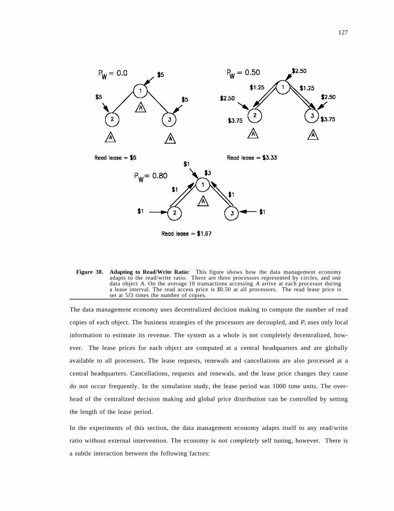
127

Figure 38. Adapting to Read/Write Ratio: This figure shows how the data management economyadapts to the read/write ratio. There are three processors represented by circles, and onedata object A. On the average 10 transactions accessing A arrive at each processor duringa lease interval. The read access price is $0.50 at all processors. The read lease price isset at 5/3 times the number of copies.

The data management economy uses decentralized decision making to compute the number of read

copies of each object. The business strategies of the processors are decoupled, and Pi uses only local

information to estimate its revenue. The system as a whole is not completely decentralized, how-

ever. The lease prices for each object are computed at a central headquarters and are globally

available to all processors. The lease requests, renewals and cancellations are also processed at a

central headquarters. Cancellations, requests and renewals, and the lease price changes they cause

do not occur frequently. In the simulation study, the lease period was 1000 time units. The over-

head of the centralized decision making and global price distribution can be controlled by setting

the length of the lease period.

In the experiments of this section, the data management economy adapts itself to any read/write

ratio without external intervention. The economy is not completely self tuning, however. There is

a subtle interaction between the following factors:

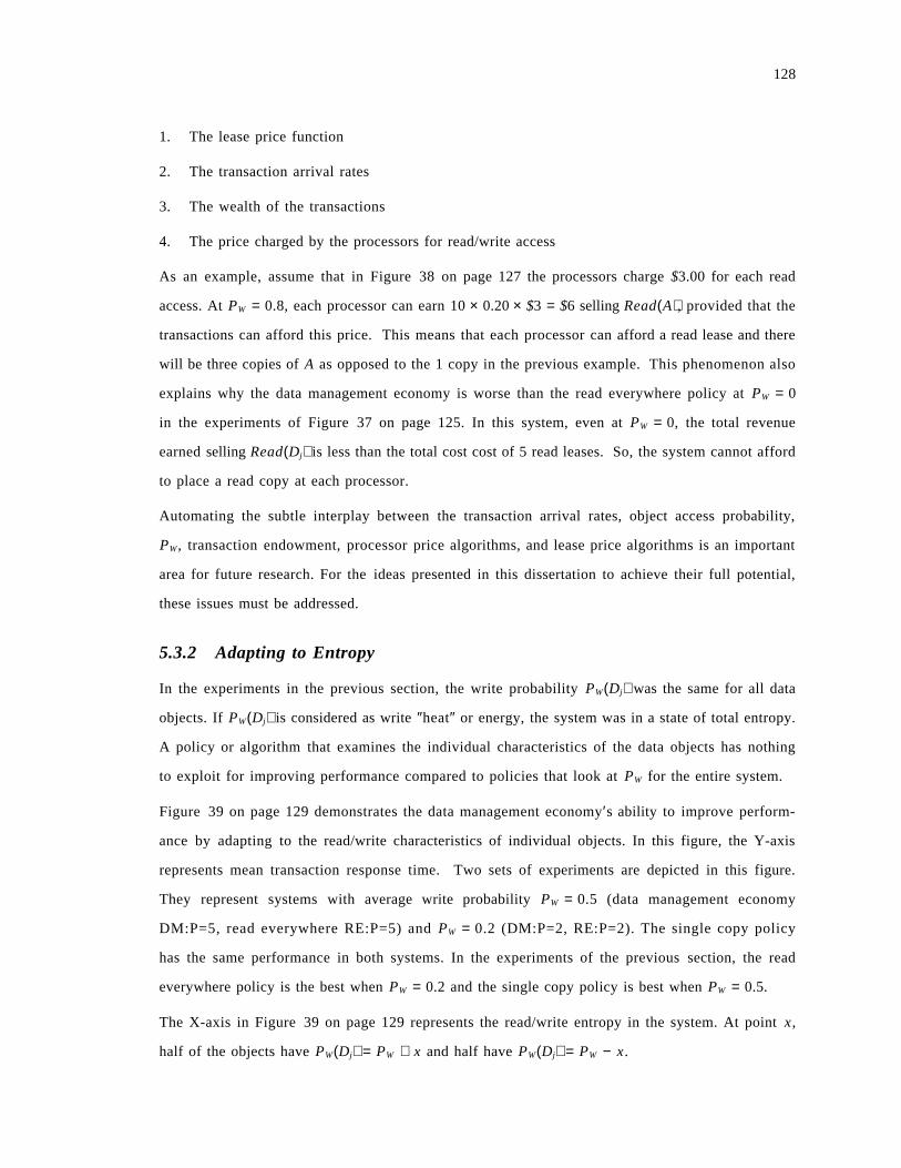
128

1. The lease price function

2. The transaction arrival rates

3. The wealth of the transactions

4. The price charged by the processors for read/write access

As an example, assume that in Figure 38 on page 127 the processors charge $3.00 for each read

access. At PW = 0.8, each processor can earn 10 × 0.20 × $3 = $6 selling Read(A), provided that the

transactions can afford this price. This means that each processor can afford a read lease and there

will be three copies of A as opposed to the 1 copy in the previous example. This phenomenon also

explains why the data management economy is worse than the read everywhere policy at PW = 0

in the experiments of Figure 37 on page 125. In this system, even at PW = 0, the total revenue

earned selling Read(Dj) is less than the total cost cost of 5 read leases. So, the system cannot afford

to place a read copy at each processor.

Automating the subtle interplay between the transaction arrival rates, object access probability,

PW, transaction endowment, processor price algorithms, and lease price algorithms is an important

area for future research. For the ideas presented in this dissertation to achieve their full potential,

these issues must be addressed.

5.3.2 Adapting to Entropy

In the experiments in the previous section, the write probability PW(Dj) was the same for all data

objects. If PW(Dj) is considered as write ″heat″ or energy, the system was in a state of total entropy.

A policy or algorithm that examines the individual characteristics of the data objects has nothing

to exploit for improving performance compared to policies that look at PW for the entire system.

Figure 39 on page 129 demonstrates the data management economy′s ability to improve perform-

ance by adapting to the read/write characteristics of individual objects. In this figure, the Y-axis

represents mean transaction response time. Two sets of experiments are depicted in this figure.

They represent systems with average write probability PW = 0.5 (data management economy

DM:P=5, read everywhere RE:P=5) and PW = 0.2 (DM:P=2, RE:P=2). The single copy policy

has the same performance in both systems. In the experiments of the previous section, the read

everywhere policy is the best when PW = 0.2 and the single copy policy is best when PW = 0.5.

The X-axis in Figure 39 on page 129 represents the read/write entropy in the system. At point x,

half of the objects have PW(Dj) = PW + x and half have PW(Dj) = PW − x.

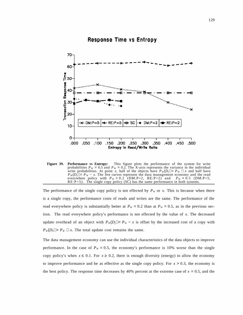
129

Figure 39. Performance vs Entropy: This figure plots the performance of the system for writeprobabilities P W = 0.5 and P W = 0.2. The X-axis represents the variance in the individualwrite probabilities. At point x, half of the objects have P W(Dj) = P W + x and half haveP W(Dj) = P W − x. The five curves represent the data management economy and the readeverywhere policy with P W = 0.2 (DM:P=2, RE:P=2) and P W = 0.5 (DM:P=5,RE:P=5) . The single copy policy (SC) has the same performance in both systems.

The performance of the single copy policy is not effected by PW or x. This is because when there

is a single copy, the performance costs of reads and writes are the same. The performance of the

read everywhere policy is substantially better at PW = 0.2 than at PW = 0.5, as in the previous sec-

tion. The read everywhere policy′s performance is not effected by the value of x. The decreased

update overhead of an object with PW(Dj) = PW − x is offset by the increased cost of a copy with

PW(Dk) = PW + x. The total update cost remains the same.

The data management economy can use the individual characteristics of the data objects to improve

performance. In the case of PW = 0.5, the economy′s performance is 10% worse than the single

copy policy′s when x ≤ 0.1. For x ≥ 0.2, there is enough diversity (energy) to allow the economy

to improve performance and be as effective as the single copy policy. For x > 0.3, the economy is

the best policy. The response time decreases by 40% percent at the extreme case of x = 0.5, and the

130

economy is 30% better than the single copy policy. At PW = 0.2, the read everywhere policy is the

best at x = 0. For x > 0.1, the data management economy is the best policy.

The experiments in this section demonstrate that the data management economy can exploit di-

versity in the read/write probabilities of the objects to improve performance relative to policies that

are based on global averages. No manual intervention is required for the economy to adapt to the

the diversity in the write probabilities.

5.3.3 Adapting to Locality

A second source of diversity that can be exploited is locality in the transactions′ reference patterns.

In the previous experiments, a transaction T arriving a node Pi accessed all of the data objects with

equal probability. Let p(i, j) denote the probability of a transaction at Pi accessing object Dj. There

are localities in the reference patterns if p(i, j) is not constant for all i and j. For example, if

p(i, j) > p(k, j) for all other processors Pk, a copy of Dj should be assigned to Pi.

Figure 40 on page 131 depicts the results of experiments to evaluate the economy′s ability to adapt

to localities in the reference patterns. The Y-axis in this figure represents mean transaction response

time. The X-axis represents the locality in the transactions′ reference patterns. At point x, the

transactions at a processor Pi exclusively access x% of the data objects. The subsets of data objects

accessed at each processor were chosen randomly. For all values of x, the mean transaction length

was 5 accesses. In this experiment, the write probability was PW = 0.4 for all objects.

The performance of the read everywhere and single copy policies do not change as a function of

locality of reference. Under the read everywhere policy, the response time of K reads on K distinct

object is the same as reading one object K times. The same is true for writes. A similar argument

holds for the single copy policy.

The data management economy′s performance improves as locality increases. For the range

100 ≥ x ≥ 60 , the response time changes by less than 10%. In the range 60 ≥ x ≥ 20 , the mean

transaction response time decreases linearly with increasing locality. At x = 20 , the economy is

30% better than the single copy policy.

Figure 41 on page 132 demonstrates how the data management economy adapts the assignment

of copies to processors based on referential locality. In this example, transactions at P1 and P2 only

update object C. Transactions at P3 only read B. Read and write access prices are $10 and the ship

price per link is $2.

131

Figure 40. Performance vs Locality of Reference: This figure plots the performance of the single copypolicy (SC), the read everywhere policy (RE) and the data management economy (DM)as a function of the locality of reference. The Y-axis represents average transaction re-sponse time. The X-axis represents the percent of the total number of data objects accessedby transactions at a given processor.

Initially, P2 is the only processor with a read copy of B. P3 subcontracts Read(B) to P1, which in turn

subcontracts to P2. Assume that 10 transactions per lease period arrive at P3. P2 earns $100 per lease

period selling Read(B), and P1 loses $110 and P3 loses $130. P1 and P3 will each order a read lease

for B (provided that the cost is less than $100). When this happens, P3 no longer subcontracts its

Read(B) business, and P1 and P2 have their Read(B) revenue fall to 0 and will not renew the read

leases on B.

In the example, the only write copy of C is at node P3. P2 subcontracts its Write(C) to P1 which in

turn subcontracts to P3. Assume that the arrival rate at processors P1 and P2 is 10 transactions per

lease period. P3 earns $200 per lease period, and P1 and P2 lose revenue of $220 and $160 respec-

tively. If the interest rate I = 0, the processors are willing to bid the following for the write copy

of C: 1) 220, 2) 160, 3) 200. So, P1 wins the next auction for the write lease of C. At this point, P1

earns $200 per lease period on Write(C) while P2 loses only $120 by not holding the lease. The write

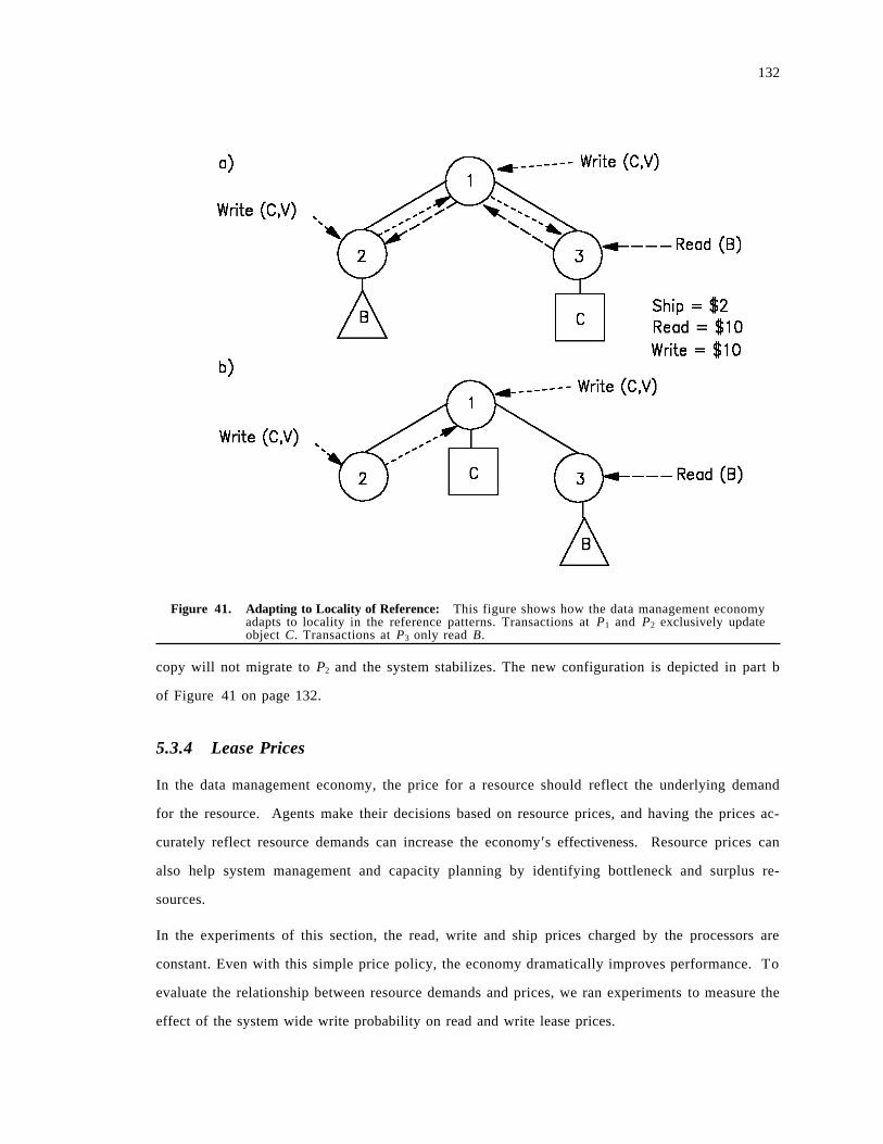
132

Figure 41. Adapting to Locality of Reference: This figure shows how the data management economyadapts to locality in the reference patterns. Transactions at P1 and P2 exclusively updateobject C. Transactions at P3 only read B.

copy will not migrate to P2 and the system stabilizes. The new configuration is depicted in part b

of Figure 41 on page 132.

5.3.4 Lease Prices

In the data management economy, the price for a resource should reflect the underlying demand

for the resource. Agents make their decisions based on resource prices, and having the prices ac-

curately reflect resource demands can increase the economy ′s effectiveness. Resource prices can

also help system management and capacity planning by identifying bottleneck and surplus re-

sources.

In the experiments of this section, the read, write and ship prices charged by the processors are

constant. Even with this simple price policy, the economy dramatically improves performance. To

evaluate the relationship between resource demands and prices, we ran experiments to measure the

effect of the system wide write probability on read and write lease prices.

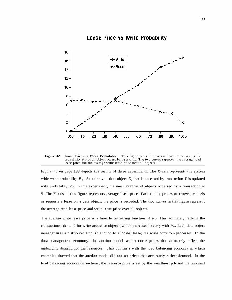
133

Figure 42. Lease Prices vs Write Probability: This figure plots the average lease price versus theprobability P W of an object access being a write. The two curves represent the average readlease price and the average write lease price over all objects.

Figure 42 on page 133 depicts the results of these experiments. The X-axis represents the system

wide write probability PW. At point x, a data object Dj that is accessed by transaction T is updated

with probability PW. In this experiment, the mean number of objects accessed by a transaction is

5. The Y-axis in this figure represents average lease price. Each time a processor renews, cancels

or requests a lease on a data object, the price is recorded. The two curves in this figure represent

the average read lease price and write lease price over all objects.

The average write lease price is a linearly increasing function of PW. This accurately reflects the

transactions′ demand for write access to objects, which increases linearly with PW. Each data object

manager uses a distributed English auction to allocate (lease) the write copy to a processor. In the

data management economy, the auction model sets resource prices that accurately reflect the

underlying demand for the resources. This contrasts with the load balancing economy in which

examples showed that the auction model did not set prices that accurately reflect demand. In the

load balancing economy′s auctions, the resource price is set by the wealthiest job and the maximal

134

wealth is not directly related to the number of jobs bidding. In the data management economy, the

number of potential bidders for a write lease is fixed. As PW increases, the wealth of each bidder

increases linearly. In the examples of Figure 22 on page 65 in the load balancing economy, if the

number of jobs remains the same and the wealth of each job increases, the sale price will also in-

creases. This explains the success of auctions in the data management economy.

Figure 42 on page 133 shows that the read lease prices do not accurately reflect the demand for read

access to data. The read demand decreases linearly with PW but the read lease price is nearly con-

stant in the interval 0 ≤ PW ≤ 0.4, and decreases nearly linearly in the interval [0.4, 0.9].

The algorithm for setting the read lease price was to charge $2 times the number of copies leased.

The write copy is also a read copy, which means that the minimum price for a pure read copy was

$2. Since the price is a function of the number of copies held, this figure shows that too few read

copies are demand when PW ≤ 0.2 and too many are held when 0.5 ≤ PW ≤ 0.9. This explains why

the economy′s performance is not as good as the read everywhere policy when 0 ≤ PW ≤ 0.2 and

is not as good as single copy with 0.5 ≤ PW ≤ 0.9. It may be possible to improve the economy′s

performance by choosing another constant for the read lease price algorithm.

The demand for read copies is not only a function of PW. The interest rate, shipping costs and

topology also effect the demand for read leases. The same is true for write lease prices. However,

there is a single write copy and the write demand aggregates over all nodes. There can be multiple

read copies and the demand is per processor as opposed to system wide. So, the read lease demand

is more subject to local considerations. Modifying the read lease price policy to account for these

problems is an area for future work that may improve the economy ′s′ performance.

5.4 Comparison with Related Work

In the performance experiments discussed in this chapter, the data management economy solves the

File Allocation Problem. We compare the data management economy with previous work on the

file allocation problem in this section. More general and extensive surveys can be found in

[33, 88].

Most previous solutions to the file allocation problem have been based on minimizing a cost

function. This approach was first used by Chu [18], and the most comprehensive cost function and

constraints are also due to Chu [19]. Under these models, there are M files (data objects) and N

processor nodes. The algorithm computes N • M binary decision variables X• . X• = 1 if a copy of

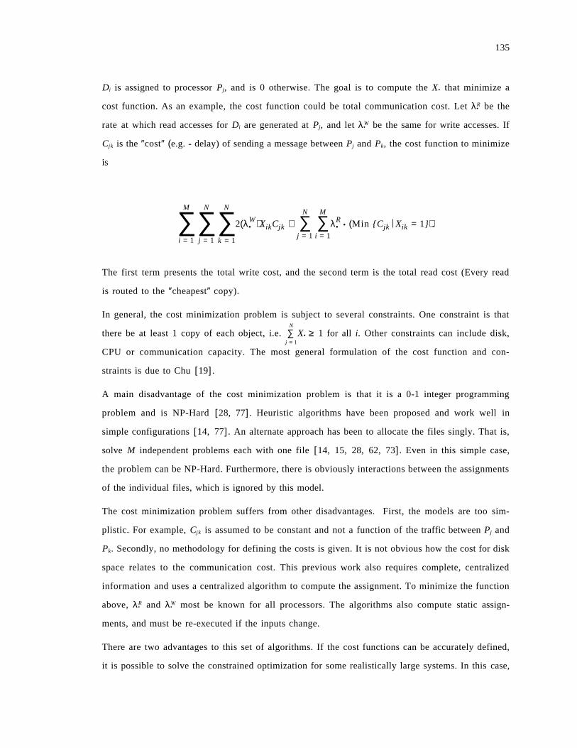
135

Di is assigned to processor Pj, and is 0 otherwise. The goal is to compute the X• that minimize a

cost function. As an example, the cost function could be total communication cost. Let λR• be the

rate at which read accesses for Di are generated at Pj, and let λW• be the same for write accesses. If

Cjk is the ″cost″ (e.g. - delay) of sending a message between Pj and Pk, the cost function to minimize

is

∑M

i = 1

∑N

j = 1

∑N

k = 1

2(λW• )XikCjk + ∑

N

j = 1∑M

i = 1

λR• • (Min {Cjk Xik = 1}).

The first term presents the total write cost, and the second term is the total read cost (Every read

is routed to the ″cheapest″ copy).

In general, the cost minimization problem is subject to several constraints. One constraint is that

there be at least 1 copy of each object, i.e. ∑N

j = 1

X• ≥ 1 for all i. Other constraints can include disk,

CPU or communication capacity. The most general formulation of the cost function and con-

straints is due to Chu [19].

A main disadvantage of the cost minimization problem is that it is a 0-1 integer programming

problem and is NP-Hard [28, 77]. Heuristic algorithms have been proposed and work well in

simple configurations [14, 77]. An alternate approach has been to allocate the files singly. That is,

solve M independent problems each with one file [14, 15, 28, 62, 73]. Even in this simple case,

the problem can be NP-Hard. Furthermore, there is obviously interactions between the assignments

of the individual files, which is ignored by this model.

The cost minimization problem suffers from other disadvantages. First, the models are too sim-

plistic. For example, Cjk is assumed to be constant and not a function of the traffic between Pj and

Pk. Secondly, no methodology for defining the costs is given. It is not obvious how the cost for disk

space relates to the communication cost. This previous work also requires complete, centralized

information and uses a centralized algorithm to compute the assignment. To minimize the function

above, λR• and λW

• most be known for all processors. The algorithms also compute static assign-

ments, and must be re-executed if the inputs change.

There are two advantages to this set of algorithms. If the cost functions can be accurately defined,

it is possible to solve the constrained optimization for some realistically large systems. In this case,

136

the assignment is provably optimal [88]. There is also evidence that heuristic algorithms do provide

near optimal assignments [33, 88].

The main advantage of the data management economy relative to the cost minimizations algo-

rithms is that the economy uses decentralized computation, and simple statistical measurement of

the parameters. Each processor independently measures λR• and λW

• . The only necessary global in-

formation are the lease prices. This information is relatively small and changes slowly. An additional

advantage of our work is that our simulation studies were based on realistic system models as op-

posed to the work above, which uses simple analytic cost functions. Finally, the data management

economy is adaptive and does not compute static solutions.

The main disadvantage of the data management economy is that currently there is no methodology

for choosing pricing functions. This is especially true for read/write access, link costs and read lease

prices. Our simulation studies indicate that very simple policies work well, however. A more thor-

ough study of pricing algorithms is an area for future work. A second disadvantage of the results

of this chapter is that the economy does not compute provably optimal assignments. Attempting

to use mathematical economics to prove optimality of the economy is also an area for further work.

The second category of solutions to the file allocation problem is based on analysis of queueing

networks [33, 88]. A global performance metric, which is usually throughput or response time, is

defined and an assignment of files to processors that optimizes the metric is computed. This work

is similar to the material above in the sense that a global metric is defined and optimized. The main

difference is that the queueing delays at CPU and communication resources are explicitly computed

instead of relying on statically defined costs.

Under this model, the file allocation problem is solved in two stages. In the first stage, a perform-

ance function Fi(x) is defined for each processor Pi. For example, Fi(x) could be the mean response

time of a file access at Pi when the arrival rate at Pi is x. The first stage algorithm computes a

branching probability pi for each node Pi. If Λ is the system wide arrival rate of file accesses (both

read and write), pi • Λ of the requests are routed to Pi. The first stage algorithm computes the

branching probabilities p*,1 p*

2, ... , p*N that minimize

∑N

i = 1

Fi(pi • Λ),

137

subject to

1. ∑N

i = 1

pi = 1

2. 0 ≤ pi ≤ 1.

The stage 1 optimization computes the processor loads that optimize the performance metric.

The second stage is to compute an assignment of files to processors that yields the desired branching

probabilities. It is typically assumed that the files are infinitely divisible [33], and 0 ≤ X• ≤ 1 instead

of X• ∈ {0, 1}. Given the branching probabilities and the distribution of access over the files com-

puting the X• is trivial.

For constrained topologies and under simplifying assumptions (exponential service time, poisson

arrival process, etc.), several algorithms have been studied that compute the optimal p*1, p*

2, ... , p*N

[4, 13, 17]. This work assumes that the distribution of accesses over all files is known, and that the

files are infinitely divisible. This means that the second stage computation is trivial.

If X• ∈ {0, 1} is required, computing the assignment in the second stage is NP-Hard [33]. Heuristic

search, linear programming and bin packing algorithms have been used to compute the X• in this

instance [31, 32].

The work above is only applicable in restricted topologies, and some assume that all references are

generated at a single node. Dowdy has extended throughput maximization to general topologies,

but optimality is no longer guaranteed [33]. This algorithm also requires solving an integer pro-

gramming problem to compute the assignments. In their survey, Dowdy and Foster demonstrate

that computing a file allocation that minimizes communication delay can be modeled as a traffic

flow assignment problem [52].

There are several disadvantages to the to the queueing based approaches to file allocation. First,

most work assumes that the data objects are infinitely divisible. If this is not the case, computing

the file assignment that yields optimal branching probabilities is NP-Hard. Secondly, most algo-

rithms can only be applied in restricted topologies (e.g. - single source of file references [76], star

networks [13, 17, 32, 45]). Third, complete information on the parameters is required and the

algorithm is centralized. Finally, the solutions are optimal only for static, steady state. The main

advantage to these algorithms is that optimality can be proven given the assumptions.

As with cost based algorithms, the data management economy has the following benefits compared

to the work above: 1) Decentralized computation, 2) More realistic system model, 3) Adaptive,

138

non-static assignments. The main disadvantages are the same as before. 1) No methodology for

pricing algorithms and 2) Not provably optimal assignments.

5.5 Conclusions

This chapter presented an economy that manages replicated data objects in a distributed transaction

processing system. Simulation based performance experiments demonstrate that the economy sub-

stantially improves performance. The economy was compared to the policies of 1) Maintaining a

single copy of each object, and 2) Maintaining a copy of each object at every processor. The

economy substantially improves performance relative to these policies.

The economy improves performance in two ways. First, the number of copies of each object is set

based on the ratio of read access to write access for the object. If writes are most common, few

copies are maintained to avoid update overhead. If, however, read access is predominant multiple

copies are maintained to ensure that reads are serviced locally or at nearby processors. The second

improvement is derived through exploiting localities in transaction access patterns. Copies of ob-

jects are assigned to the processors at which they are most frequently accessed. We provided several

examples that illustrate how the economy uses supply and demand to achieve the performance

improvements.

The data management economy solves the File Allocation Problem. We presented a brief survey

of previous work on this problem, and compared it with the economy. The main advantages of the

data management economy relative to previous work are: 1) Decentralized decision making, 2)

Realistic system models, 3) Computational tractability. The main disadvantage is that the econo-

my′s assignments are not provably optimal.

We studied the relationship between resource prices and demand. In this economy, an English

auction model was shown to set lease prices for write copies that accurately reflect the demand for

write access. Our algorithm for setting read lease prices was shown to be less successful. We are

currently exploring alternative policies.

Several avenues for further work were presented. The interactions between the processors ′ and data

object managers′ pricing algorithms and the transaction endowments that should be addressed. We

used simple pricing algorithms in our experiments. More sophisticated policies may be able to fur-

ther improve performance. Finally, our economy is not currently compatible with concurrency

139

control based on locking. Incorporating concurrency control is necessary to more realistically model

transaction processing systems.

140

6.0 Summary and Directions for Future Work

This thesis studied resource sharing problems in distributed computer systems. We proposed that

a distributed system should be structured as a society of competing microeconomic agents. We

demonstrated the effectiveness and generality of this approach by applying our ideas to the diverse

problems of load balancing, flow control in virtual circuit networks, and data management.

Our load balancing economy improved mean job waiting time compared to a representative, non-

economic load balancing algorithm. We showed that our economy implements a broad spectrum

of load balancing strategies. At one extreme, the economy has a high migration rate and migrates

short jobs. At the other extreme, the economy migrates long jobs and has a low migration rate.

We demonstrated that the economy′s load balancing strategy can be tuned to relative speeds of

CPU vs communication and that this gives better performance. The economy was shown to im-

plement flow control by decreasing throughput to improve response time. We also evaluated the

effectiveness of job wealth as a priority mechanism. Our experiments revealed that a simple learning

mechanism for the jobs substantially improved performance and counter acted the effectiveness of

wealth as a priority mechanism. Finally, we showed how the economy limits complexity by being

inherently decentralized and modular.

The flow control economy demonstrated how economies effectively deal with diversity. Each user

of a virtual circuit can independently set its individual throughput-delay goals. This improves on

previous work which has either: 1) Defined a system wide throughput-delay goal, or 2) Has as-

sumed all circuits have the same throughput-delay goals (e.g. - Maximize throughput). We pro-

posed Pareto-optimality as a new definition for optimal resource allocations for the flow control

problem. We presented a formalization of fairness criteria and compared Pareto-optimality with

previous definitions of optimality and fairness. We extended tools provided by mathematical eco-

nomics and proved that the resource allocations computed by our economy are Pareto-optimal.

We also proved that a Pareto-optimal allocation exists for arbitrary network. Proving convergence

in an economy is an extremely difficult problem, and we did not prove convergence for the flow

control economy. An extensive simulation study demonstrated that the economy rapidly converged

to an optimal allocation over a broad set of network parameters. We also discussed the integration

of circuit routing with flow control. The flow control economy demonstrated the power of math-

ematical economics as a tool for modelling resource sharing problems in distributed computer sys-

141

tems. It also demonstrated that the models must be altered to realistically model the computer

systems.

The data management economy solved a general version of the file allocation problem. This econ-

omy improved mean transaction response time compared to simple system wide policies. The im-

provements were achieved in two ways. First, the number of copies of a data object was chosen

based on the ratio of write access to read access. Secondly, localities in transaction reference patterns

were detected and exploited. The economy was tested on a more realistic system model that pre-

vious work. This economy demonstrated how economic competition resolves conflicting goals.

There is a trade-off for the number of copies of an object in the system. Many copies decreases read

access time, but increases write access time. A single copy eliminates update overhead, but increases

read access time. The economy resolved these conflicts over a broad range of read/write ratios. The

data management economy and the examples from this chapter highlighted the importance of the

algorithms that set resource prices. Our experiments demonstrate the simple policies work well.

Finally, the data management economy demonstrated that economic models can efficiently allocate

logical resources (access to data).

This thesis opens up several opportunities for further work. This work falls into two categories.

The first are extensions to the economies presented in this thesis. The load balancing economy ex-

periments showed that the economy can have its load balancing strategy tuned for a specific ratio

of CPU to communication power. This tuning requires manual intervention, however. Automating

the tuning is a possible area for further work. We also discussed that the economy implements flow

control. Currently there is no mechanism for setting the desired throughput-response goal. Provid-

ing such a facility is an area for future research. Two avenues for work are left open by the flow

control economy. The first is proof of convergence of the tatonement process or a counter exam-

ple. The second is integration of alternate models of VC throughput-delay goals. Our model is very

general, but does not exhaust the set of possible goals. Finally, the data management economy has

three opportunities for more research. One is determining if more complex price setting algorithms

improve performance. Secondly, it was shown that there are interactions between the transactions′

endowments, the processors′ pricing algorithms and the data managers′ pricing algorithms. Auto-

matically resolving these interactions would enhance the usefulness of the economy. The final

possible extension of the data management economy is including concurrency control in the econ-

omy.

142

The second avenue for further work is applying the microeconomic paradigm to other problems in

distributed systems. Doing so will further demonstrate the generality of this approach. In this thesis

we focused on the performance achieved by resource sharing algorithms. It may be possible to apply

this approach to problems of reliability and error recovery. Finally, an extremely promising area for

research is further relaxing the assumptions made by mathematical economics. This will allow

modelling a broader set of distributed system problems. The two most important assumptions are:

1) Agents possess complete, apriori knowledge of their resource requirements. 2) The set of agents

is fixed. Overcoming these assumptions is an interesting theoretical challenge, and would provide

computer science with a powerful new set of tools.

143

Bibliography

[1] Kenneth J. Arrow and Michael D. Intrilligator, editor. Hand-

book of Mathematical Economics.

North-Holland Publishing Co., Amsterdam, 1981.

[2] N. Abramson.

The ALOHA System - Another Alternative for Com-

puter Communication.

Proceedings AFIPS Fall Joint Computer Conference,

pages 281-285, AFIPS Press, Montvale, NJ, 1970.

[3] N. Abramson.

The Throughput of Packet Broadcasting Channels.

IEEE Transactions on Communications, COM-25(1),

January 1977.

[4] S. R. Arora and A. Gallo.

Optimal Sizing, Loading and Reloading in a Multi-level

Memory Hierarchy SysteM.

Proceedings AFIPS 1971 Spring Joint Computer Confer-

ence, 38, 1971.

[5] K. Arrow and F. Hahn.

General Competitive Analysis.

Holden Day Publisher, San Francisco, 1971.

[6] Amnon Barak and Amnon Shiloh.

A Distributed Load Balancing Policy for a Multicom-

puter.

Software Practice and Experience, 15(9):901-913, Septem-

ber 1985.

[7] Phillip A. Bernstein and Nathan Goodman.

Concurrency Control in Distributed Database Systems.

Computing Surveys, 13(2), June 1981.

[8] Philip A. Bernstein, Vassos Hadzilacos and Nathan Goodman.

Concurrency Control and Recovery in Database Systems.

Addison-Wesley, Reading, MA, 1987.

[9] Dimitri Bertsekas and Robert Gallager.

Data Networks.

Prentice-Hall, Englewood Cliffs, NJ, 1987.

[10] Kadaba Bharath-Kumar and Jeffrey Jaffe.

A New Approach to Performance Oriented Flow Con-

trol.

IEEE Transactions on Communication, COM-29(4), April

1981.

[11] Andreas Bovopoulos and Aurel Lazar.

Decentralized Algorithms for Optimal Flow Control.

Proceedings of the 25th Annual Allerton Conference on

Communication, Control and Computing, September

1987.

[12] Raymond M. Bryant and Raphael A. Finkel.

A Stable Distributed Scheduling Algorithm.

Proceedings of the Second International Conference on

Distributed Computing Systems, pages 314-232, April

1981.

[13] J. P. Buzen and P. Chen.

Optimal Load Balancing in Memory Hierarchies.

Proceedings of IFIP, North-Holland, Amsterdam, 1974.

[14] R. G. Casey.

Allocation of Copies of a File in an Information Net-

work.

Proceedings AFIPS 1972 Spring Joint Computer Confer-

ence, AFIPS Presss, Arlington VA, 1972.

144

[15] K. M. Chandy and J. E. Hewes.

File Allocation in Distributed Systems.

Proceedings International Symposium on Computer Per-

formance Modeling, Measurement and Evaluation, March

1976.

[16] D. Chazan and W. Miranker.

Chaotic Relaxation.

Linear Algebra and Its Applications, 2, 1969.

[17] P. Chen.

Optimal File Allocation in Multilevel Storage Systems.

Proceedings of AFIPS 1973 National Computer Confer-

ence, 42, 1973.

[18] Wesley W. Chu.

Optimal File Allocation in a Multiple Computer System.

IEEE Transactions on Computers, C-18(10), October

1969.

[19] Wesley W. Chu.

Optimal File Allocation in Computer Networks.

in N. Abramson and F.F. Kuo, editor, Computer-

Communication Systems, Prentice-Hall, Englewood

Cliffs, NJ, 1973.

[20] E.F. Codd.

A Relational Data Model for Large Shared Data Banks.

CACM , 13(6), June 1970.

[21] C.J. Date.

An Introduction to Database Systems: Volume I.

Addison-Wesley Publishing Co., Reading, Mass., 1982.

[22] Randall Davis and Reid G. Smith.

Negotiation as a Metaphor for Distributed Problem

Solving.

Artificial Intelligence, 20:63-109, 1983.

[23] Harvey M. Deitel.

An Introduction to Operating Systems.

Addison-Wesley Publishing Co., Reading, MA, 1984.

[24] K. Eric Drexler and Mark S. Miller.

Incentive Engineering for Computational Resource Man-

agement.

in B. A. Huberman, editor, The Ecology of Computation,

North-Holland, Amsterdam, 1988.

[25] Alex Dupuy.

Network Simulation Testbed (NEST) User Manual.

Computer Science Dept. , Columbia

University CS-NEST, 1986.

[26] Derek L. Eager, D. Lazowska and John Zahorjan.

Adaptive Load Sharing in Homogeneous Distributed

Systems.

IEEE Transactions on Software Engineering, SE-12(5),

May 1986.

[27] Derek L. Eager, Edward D. Lazowska and John Zahorjan.

A Comparison of Receiver-Initiated and Sender-Initiated

Dynamic Load Sharing.

Dept. of Computer Science University of

Washington 85-04-01, April 1985.

[28] Kapali P. Eswaran.

Placement of Records in a File and File Allocation in a

Computer Network.

Proceedings IFIP Conference, Stockholm, Sweden, Au-

gust 1974.

[29] Donald F. Ferguson.

Dynamic Distributed Load Sharing Algorithms - A Sur-

vey.

Computer Science Dept., Columbia University, May

1985.

145

[30] Domenico Ferrari.

Computer Systems Performance Evaluation.

Prentice-Hall, Inc., Englewood Cliffs, New Jersey, 1978.

[31] D.V. Foster and J.C. Browne.

File Assignment in Memory Hierarchies.

Proceedings Modeling and Performance Evaluation of

Computer Systems, North-Holland, October 1976.

[32] D.V. Foster, L.W. Dowdy and J.E. Ames.

File Assignment in a Computer Network.

Computer Networks, 5:341-349, September 1981.

[33] Lawrence Dowdy and Derrell Foster.

Comparative Models of the File Assignment Problem.

Computing Surveys, 14(2), June 1982.

[34] C.J. Gao, J.W. Liu and M Riley.

Load Balancing Algorithms in Homogeneous Distributed

Systems.

Proceedings of the 13th International on Parallel Process-

ing, 1984.

[35] C.J. Gao, J.W. Liu and M Riley.

Load Balancing Algorithms in Homogeneous Distributed

Systems.

University of Illinois at

Urbana-Champaign UIUC-DCS-84-1168, 1984.

[36] Lionel M. Ni and Ching-Wei Xu and Thomas B. Gendreau.

A Distributed Drafting Algorithm for Load Balancing.

IEEE Transactions on Software Engineering, SE-11(10),

October 1985.

[37] Mario Gerla and Leonard Kleinrock.

Flow Control: A Comparative Survey.

IEEE Transactions on Communication, COM-28(4), April

1980.

[38] G.M. Heal.

Planning Without Prices.

Review of Economic Studies, 36:346-362, 1969.

[39] G.M. Heal.

The Theory of Economic Planning.

North-Holland Publishing Co., Amsterdam, 1973.

[40] W. Hildenbrand and A.P. Kirman.

Introduction to Equilibrium Analysis.

North-Holland Publishing Co., Amsterdam, 1976.

[41] Y.C. Ho, L. Servi and R. Suri.

A Class of Center-Free Resource Allocation Algorithms.

Large Scale Systems, 1:51-62, 1980.

[42] Man-Tung Tony Hsiao.

Optimal Decentralized Flow Control in Computer Com-

munication Networks.

PhD thesis, Center for Telecommunications Research,

Columbia University, New York, NY. 86.

[43] Man-Tung Hsiao and Aurel Lazar.

A Game Theoretic Approach to Optimal Decentralized

Flow Control of Markovian Queueing Networks with

Multiple Controllers.

Proceedings of Performance ′87, Brussels, Belgium, De-

cember 1987.

[44] Chi-Yin Huang Hsu and Jane W.-S Liu.

Dynamic Load Balancing Algorithms in Homogeneous

Distributed Systems.

Proceedings of 6th IEEE Distributed Computer Systems

Conference, 1986.

146

[45] P.H. Hughes and G. Moe.

A Structural Approach to Computer Performance.

Analysis Proceedings AFIPS 1973 Spring Joint Computer

Conference, AFIPS Press, Arlington, VA, 1973.

[46] K. Hwang et al.

Engineering Computer Network (ECN): A Hard Wired

Network of Unix Computer Systems.

Proceedings of the National Computer Conference, May

1981.

[47] K. Hwang et al.

A Unix Based Local Computer Network with Load Bal-

ancing.

IEEE Computer, April 1982.

[48] Jeffrey Jaffe.

Bottleneck Flow Control.

IEEE Transactions on Communication, COM-29(7), July

1981.

[49] Jeffrey Jaffe.

Flow Control Power is Nondecentralizable.

IEEE Transactions on Communication, COM-29(9), Sep-

tember. 1981.

[50] R. E. Kahn.

The Organization of Computer Resources into a Packet

Radio Network.

IEEE Transactions on Communications, COM-25(1),

January 1977.

[51] Leonard Kleinrock.

Queueing Systems: Volume I: Theory.

Wiley Interscience, New York, 1975.

[52] Leonard Kleinrock.

Queueing Systems: Volume II: Computer Applications.

Wiley Interscience, New York, 1975.

[53] Phillip Krueger and Raphael A. Finkel.

An Adaptive Load Balancing Algorithm for a Multicom-

puter.

University of Wisconsin, Madison 539, April 1984.

[54] Phillip Krueger and Miron Livny.

When it the Best Load Sharing Algorithm a Load Bal-

ancing Algorithm?.

University of Wisconsin, Madison, April 1987.

[55] James F. Kurose.

Time-Constrained Communication in Multiple Access

Networks.

PhD thesis, Columbia University, 1984.

[56] James F. Kurose, Mischa Schwartz and Yechiam Yemini.

Distributed Multiple Access Protocols and Real-Time

Communication.

Computing Surveys, 6(1), March 1984.

[57] James F. Kurose, Mischa Schwartz and Yechiam Yemini.

A Microeconomic Approach to Optimization of Channel

Access Policies in Multiaccess Networks.

Proceedings of the 5th IEEE Distributed Computer Sys-

tems Conference, pages 70-80, May 1985.

[58] James F. Kurose and Rahul Simha.

A Microeconomic Approach to Optimal File Allocation.

Proceedings of the 6th IEEE Distributed Computer Sys-

tems Conference, 1986.

[59] James F. Kurose and Rahul Simha.

Second Derivative Algorithms for Optimal Resource Al-

location in Distributed Computer Systems.

Proceedings of the 7th International Conf. on Distributed

Computing Systems, 1987.

147

[60] James F. Kurose and Rahul Simha.

A Microeconomic Approach to Optimal Resource Allo-

cation in Distributed Computer Systems.

Univ. of Mass. at Amherst, 1987.

Submitted to IEEE Transactions on Computers.

[61] L. Lamport, R. Shostak and M. Pease.

The Byzantine Generals Problem.

ACM Transactions on Programming Languages and Sys-

tems, 4(3):382-401, 1982.

[62] K.D. Levin and H.L. Morgan.

Optimizing Distributed Databases - A Framework for

Research.

Proceedings AFIPS 1975 National Computer Conference,

44, 1975.

[63] S. Li and T. Basar.

Distributed Algorithms for the Computation of Nonco-

operative Criteria.

Automatica, 23(4), July 1987.

[64] Miron Livny.

The Study of Load Balancing Algorithms for Decentralized

Distributed Processing Systems.

PhD thesis, Weizmann Institue of Science, Rehovot,

Israel. 1984.

[65] Miron Livny and Myron Melman.

Load Balancing in Homogeneous Distributed Systems.

Proceedings of the ACM Computer Networking Perform-

ance Symposium, pages 47-55, April 1982.

[66] Thomas W. Malone, Richard E. Fikes, Kenneth R. Grant and

Michael T. Howard.

Market Like Load Sharing in Distributed Computing

Environments.

MIT, 1987.

[67] Thomas W. Malone, Richard E. Fikes, Kenneth R. Grant and

Michael T. Howard.

Enterprise: A Market-Like Task Scheduler for Distrib-

uted Computing Environments.

in B. A. Huberman, editor, The Ecology of Computation,

North-Holland, Amsterdam, 1988.

[68] M. Martinez.

Program behavior prediction and prefetching.

Acta Informatica, 17:101-120, 1982.

[69] Christos Douglieris and Ravi Mazumdar.

On Pareto Optimal Flow Control in a Multiclass Envi-

ronment.

Center for Telecommunications Research, Columbia

University, 1987.

[70] Christos Douglieris and Ravi Mazumdar.

User Optimal Flow Control in an Integrated Environ-

ment.

CTR Technical Report, Columbia University, 1987.

[71] R.M. Metcalfe and D.R. Boggs.

Ethernet: Distributed Packet Switching for Local Com-

puter Networks.

Xerox csl-80-2, 1980.

[72] Mark S. Miller and K. Eric Drexler.

Markets and Computation: Agoric Open Systems.

in B. A. Huberman, editor, The Ecology of Computation,

North-Holland, Amsterdam, 1988.

[73] H.L. Morgan and K.D. Levin.

Optimal Program and Data Locations in Computer Net-

works.

Communications of the ACM, 20(5):124-130, May 1977.

148

[74] Yung-Terng Wang and Robert J. Morris.

Load Sharing in Distributed Systems.

IEEE Transactions on Computers, C-34(3), March 1985.

[75] M.L. Powell and B.P. Miller.

Process Migration in DEMOS/MP.

Proceedings of 9th ACM Symposium on Operating Sys-

tems Principles, 1983.

[76] C. V. Ramamoorthy and K. M. Chandy.

Optimization of Memory Hierarchies in Multipro-

grammed Systems.

Journal of the ACM, 17(3), July 1970.

[77] C. V. Ramamoorthy and B. W. Wah.

The Isomorphism of Simple File Allocation.

IEEE Transactions on Computers, C-32(3), March 1983.

[78] Beverly Sanders.

An Incentive Compatible Flow Control Algorithm for

Fair Rate Allocation in Computer/Communication Net-

works.

Proceedings of the 6th IEEE Distributed Computer Sys-

tems Conference, pages 314-320, May 1986.

[79] Beverly Sanders.

An Asynchronous, Distributed Flow Control Algorithm

for Rate Allocation in Computer Networks.

IEEE Transactions on Computers, C-37(7), July 1988.

[80] Herbert Scarf.

The Computation of Economic Equilibria.

Yale University Press, New Haven, CN, 1973.

[81] Mischa Schwartz.

Telecommunication Networks: Protocols, Modeling and

Analysis.

Addison-Wesley Publishing Co., Reading, Mass., 1987.

[82] Martin Shubik.

Game Theory in the Social Sciences.

The MIT Press, Cambridge, Mass., 1983.

[83] Reid G. Smith.

The Contract Net Protocol: High Level Communication

and Control in a Distributed Problem Solver.

IEEE Transactions on Computers, C-29(12), December

1980.

[84] Reid G. Smith and Randall Davis.

Applications of the Contract Net Framework: Distrib-

uted Sensing.

Proceedings ARPA Distributed Sensor Network Sympo-

sium, pages 12-20, December 1978.

[85] Reid G. Smith and Randall Davis.

Frameworks for Cooperating in Distributed Problem

Solving.

IEEE Transactions on Systems, Man and Cybernetics,

SMC-11(1), January 1981.

[86] John A. Stankovic.

Stability and Distributed Scheduling Algorithms.

IEEE Transactions on Software Engineering, SE-11(10),

October. 1985.

[87] Harold S. Stone.

Multiprocessor Scheduling with the Aid of Network Flow

Algorithms.

IEEE Transactions on Software Engineering, SE-3(1),

January 1977.

[88] Benjamin Wah.

File Placement on Distributed Computer Systems.

Computer, 17(1), January 1984.

149

[89] Yechiam Yemini.

Selfish Optimization in Computer Networks.

Proceedings of the 20th IEEE Conference on Decision and

Control, pages 281-285, IEEE, San Diego, December

1981.

[90] Yechiam Yemini and Leonard Kleinrock.

On a General Rules for Access Control or Silence is

Golden....

Proceedings of the International Conference on Flow

Control in Computer Networks, pages 335-347, North

Holland Press Amsterdam, Versailles, February 1979.

[91] Songnian Zhou and Domenico Ferrari.

A Measurement Study of Load Balancing Performance.

Proceedings of 7th International Conference on Distrib-

uted Computing Systems, 1987.