Micro-Randomized Trials in mHealth

Peng Liao ∗1, Predrag Klasnja2, Ambuj Tewari1, and Susan A. Murphy1

1Department of Statistics, University of Michigan, Ann Arbor, MI 481092School of Information, University of Michigan, Ann Arbor, MI 48109

April 2, 2015

Abstract

The use and development of mobile interventions is experiencing rapid growth. In “just-in-time” mobileinterventions, treatments are provided via a mobile device that are intended to help an individual make healthydecisions “in the moment,” and thus have a proximal, near future impact. Currently the development of mobileinterventions is proceeding at a much faster pace than that of associated data science methods. A first steptoward developing data-based methods is to provide an experimental design for use in testing the proximaleffects of these just-in-time treatments. In this paper, we propose a “micro-randomized” trial design for thispurpose. In a micro-randomized trial, treatments are sequentially randomized throughout the conduct of thestudy, with the result that each participant may be randomized at the 100s or 1000s of occasions at which atreatment might be provided. Further, we develop a test statistic for assessing the proximal effect of a treatmentas well as an associated sample size calculator. We conduct simulation evaluations of the sample size calculatorin various settings. Rules of thumb that might be used in designing the micro-randomized trial are discussed.This work is motivated by our collaboration on the HeartSteps mobile application designed to increase physicalactivity.

Key words: Mirco-randomized Trial, Sample Size Calculation, mHealth

1 Introduction

The use and development of mobile interventions is experiencing rapid growth. Mobile interventions areused across the health fields and include treatments used to improve HIV medication adherence [11, 14], toimprove activity [12], accompany counseling/pharmacotherapy in substance use [4, 18], reinforce abstinence inaddictions [1, 2] and to support recovery from alcohol dependence [9, 21]. Mobile interventions in maintainingadherence to anti-retroviral therapy and smoking cessation have shown sufficient effectiveness and replicabilityin trials and thus have been recommended for inclusion in health services [8].

However as Nilsen et al. [20] state “In fact, the development of mHealth technologies is currently progressingat a much faster pace than the science to evaluate their validity and efficacy, introducing the risk that ineffectiveor even potentially harmful or iatrogenic applications will be implemented.”Indeed reviews, while reporting pre-liminary evidence of effectiveness, call for more programmatic, data-based approaches to constructing mobileinterventions [8, 19]. In particular these reviews call for research that focuses on data-informed developmentof these complex multi-component interventions prior to their evaluation in standard randomized controlledtrials. But methods for using data to inform the design and evaluation of adaptive mobile interventions havelagged behind the use and deployment of these interventions [13, 20, 26].

Many mobile interventions are designed to be “just-in-time” interventions, meaning that they intend toprovide treatments that help an individual make healthy decisions in the moment, such as engaging in adesirable behavior (e.g., taking a medication on time) or effectively coping with a stressful situation. As such,mobile interventions are often intended to have proximal, near-term effects. A first approach toward developingdata-based methods for evaluation of mobile health interventions is to provide an experimental design for usein testing the proximal effects of the treatments. This paper proposes a micro-randomized trial design for thispurpose. In a micro-randomized trial, treatments are sequentially randomized throughout the conduct of thestudy, with the result that each participant may be randomized at the hundreds or thousands of occasions atwhich a treatment might be provided. This repeated randomization of treatments under investigation enablescausal modeling of each treatment’s time-varying proximal effect as well as modeling of time-varying effect

∗Corresponding author. 439 West Hall, 1085 South University Ave, Ann Arbor, MI 48109. Email:pengliao@umich.edu

1

arX

iv:1

504.

0023

8v1

[st

at.M

E]

1 A

pr 2

015

moderation. Thus, the micro-randomized trial can be seen as a first experimental step in the developmentof effective mobile interventions that are composed of sequences of treatments. We propose to size the trialto detect the proximal main effect of the treatments. This is akin to the use of factorial designs for use inconstructing multi-component interventions. In these factorial designs [3, 6], a first analysis often involvestesting if the main effect of each treatment is equal to 0.

This work is motivated by our collaboration on the HeartSteps mobile application for increasing physicalactivity, which we will use to illustrate our discussion. One of the treatments in HeartSteps is suggestions forphysical activity which are tailored to the person’s current context. HeartSteps can deliver these suggestionsat any of the five time intervals during the day, which correspond roughly to morning commute, mid-day,mid-afternoon, evening commute, and post-dinner times. When a suggestion is delivered, the user’s phoneplays a notification sound, vibrates and lights up, and the suggestion is displayed on the lock screen of the phone.These suggestions encourage activity in the current context and are intended to have an effect (getting a personto walk) within the next hour.

In the following section, we introduce the micro-randomized trial design. In section 3 we precisely definethe proximal main effect of a treatment, using the language of potential outcomes. We develop the test statisticfor assessing the proximal effect of a treatment as well as an associated sample size calculator in section 4 and 5.Next we provide simulation evaluation of the sample size calculator. We end, in Section 7, with a discussion.

2 Micro-Randomized Trial

In general an individual’s longitudinal data, recorded via mobile devices that sense and provide treatments, canbe written as

{S0,S1, A1,S2, A2, . . . ,St , At , . . . ,ST , AT ,ST+1}

where, t indexes decision times, S0 is a vector of baseline information (gender, ethnicity, etc.) and St (t ≥ 1) isinformation collected between time t −1 and t (e.g. summary measures of recent activity levels, engagement,and burden; day of week; weather; busyness indicated by smartphone calendar, etc.). The treatment at time t isdenoted by At ; throughout this paper we consider binary options for the treatments (e.g., the treatment is onor off). The proximal response, denoted by Yt+1, is a known function of {St , At ,St+1}. Here we assume that thelongitudinal data are independent and identically distributed across N individuals. Note that this assumptionwould be violated, if for example, some of the treatments are used to enhance social support between individualsin the study.

In HeartSteps, data (St ) is collected both passively via sensors and via participant self-report. Each participantis provided a “Jawbone” band [5], worn at the wrist, which collects daily step count and the amount of sleep theuser had the previous night. Furthermore sensors on the phone are used to collect a variety of information ateach of the 5 time points during the day, including the time-stamp, location, busyness of planned activities onthe phone calendar and other activity on the phone. Each evening, self-report data is collected including utilityand burden ratings. The proximal response, Yt+1, for activity suggestions is the step count in the hour followingtime t .

A decision time is a point in time at which—based on participant’s current state, past behavior, or currentcontext—treatment may need to be delivered. Decision times vary by the nature of the intervention component.In HeartSteps, the decision times for activity suggestions are 5 times per day over the 42 day study duration.For an alcohol-recovery application that provides an intervention when an individual goes within 10 feet of ahigh risk location (e.g. a liquor store), decision points might be every 2 minutes, the frequency at which theapplication would get the person’s current location and assess whether she is close to a high-risk location. Ina long-term study of an intervention for multiple health behaviors, the decision points might be weekly ormonthly at which times, decisions are made regarding whether to change the focus from one behavior (e.g.,physical activity) to another (e.g., diet). Finally, in many studies there is an option for an individual to press a"panic”button, indicating the need for help; for such interventions, decision times correspond to times at whichthe panic button might be pressed.

A micro-randomized trial is a trial in which at each decision time t , participants are randomized to atreatment option, denoted by At . Treatment options may correspond to whether or not a treatment is providedat a decision time; for example in HeartSteps, whether or not the individual is provided a lock-screen activitysuggestion. Or treatment options may be alternative types of treatment that can be provided at the same decisiontime; for example, a daily step goal treatment might have two options, a fixed 10,000-steps-a-day goal or anadaptive goal based on the user’s activity level on the previous day. Considerations of treatment burden oftenimply that the randomization will not be uniform. For example in HeartSteps, P [At = 1] = .4 so that, if anindividual is always available, on average 2 lock-screen activity messages are delivered per day.

2

In designing, that is, determining the sample size for, a micro-randomized trial we focus on the reducedlongitudinal data

{S0, I1, A1,Y2, I2, A2,Y3, . . . , It , At ,Yt+1, . . . , IT , AT ,YT+1}.

The variable, It is an “availability”indicator. The availability indicator is coded as It = 1 if the individual isavailable for treatment and It = 0 otherwise. At some decision times feasibility, ethics or burden considerationsmean that the individual is unavailable for treatment and thus At should not be delivered. Consider againHeartSteps: if sensors indicate that the individual is likely driving a car or the individual is currently walking,then the lock-screen activity message should not occur. Other examples of when individuals are unavailable fortreatment include: in the alcohol recovery setting, an “warning”treatment would only be potentially providedwhen sensors indicate that the individual is within 10 feet of a high risk location or a treatment might only beprovided if the individual reports a high level of craving. If the application has a panic button, then only in anx second interval in which the panic button is pressed is it appropriate to provide “panic button”treatments.Individuals may be unavailable for treatment by choice. For example, the HeartSteps application permits theindividual to turn off the lock-screen activity messages; this option is considered critical to maintaining partici-pant buy-in and engagement with HeartSteps. After viewing the lock-screen activity message, the individualhas the option of turning off the lock-screen message for 4 or 8 or 12 hours. After the specified time interval,the lock-screen message automatically turns on again. To summarize, the availability indicator at time t is theindicator for the subpopulation at time t among which we are interested in assessing the proximal main effect ofthe treatment; we are uninterested in assessing the proximal main effect of a treatment among individuals forwhom it is unethical to provide treatment or for whom it makes no scientific sense to provide treatment or amongthose who refuse to be provided a treatment.

3 Proximal Main Effect of a Treatment

As discussed above, treatments in mobile health interventions are often designed so as to have a proximaleffect (e.g., increase activity in near future, help an individual manage current cravings for drugs or food, takemedications on schedule, etc.). As a result, a first question in developing a mobile health intervention is whetherthe treatments have a proximal effect. Here we develop sample size formulae that guarantee a stated power todetect the proximal effect of a treatment. In particular we aim to test if the proximal main effect is zero.

To define the proximal main effect of a treatment, we use potential outcomes [22, 23, 25]. Our use ofpotential outcome notation is slightly more complicated than usual because treatment can only be providedwhen an individual is available. As a result, we index the potential outcomes by decision rules that incorporateavailability. In particular define d(a, i ) for a ∈ {0,1}, i ∈ {0,1} by d(a,0) =“unavailable-do nothing”and d(a,1) = a.Then for each a1 ∈ A1 = {0,1}, define D1(a1) = d(a1, I1). Then we denote the potential proximal responsesfollowing decision time 1 by {Y D1(1)

2 , Y D1(0)2 } and denote the potential availability indicators at decision time 2

by {I D1(1)2 , I D1(0)

2 }. Next for each a2 = (a1, a2) with a1, a2 ∈ {0,1}, define D2(a2) = d(a2, I D1(a1)2 ). Define D2(a2) =

(D1(a1),D2(a2)). A potential proximal response following decision time 2 and corresponding to a2 is Y D2(a2)3

and a potential availability indicator at decision time 3 is I D2(a2)3 . Similarly, for each at = (a1, . . . , at ) ∈ At =

{(a1, . . . , at )∣∣ai ∈ {0,1}, i = 1, . . . , t }, define D t (at ) = d(at , I D t−1(at−1)

t ) and D t (at ) = (D1(a1), . . . ,D t (at )). For each

at = (a1, . . . , at ) ∈At , the potential proximal response is Y D t−1(at−1)t (following decision time t −1) and potential

availability indicator is I D t−1(at−1)t at decision time t .

We define the proximal main effect of a treatment at time t among available individuals by:

β(t ) = E

(Y D t (At−1,1)

t+1 −Y D t (At−1,0)t+1

∣∣∣I D t−1(At−1)t = 1

)where the expectation is taken with respect to the distribution of the potential outcomes and randomization inAt−1. This proximal effect is conditional in that the effect of treatment at time t is defined for only individuals

available for treatment at time t , that is, I D t−1(At−1)t = 1. This proximal effect is a main effect in that the effect is

marginal over any effects of At−1. The former conditional aspect of the definition is related to the concept ofviable or feasible dynamic treatment regimes [24, 28] in which one assesses only the causal effect of treatmentsthat can actually be provided.

Consider the proximal main effect, β(t), as t varies across time. β(t) may vary across time for a variety ofreasons. To see this consider the case of HeartSteps. Here β(t) might initially increase with increasing t asparticipants learn and practice the activities suggested on the lock-screen. For larger t one might expect to see

3

decreasing or flat β(t) due to habituation (participants begin to, at least partially, ignore the messages). Thistime variation in β(t ) can be attributed to both the immediate effect of a lock-screen activity message as well asinteractions between the past lock-screen activity messages and the present activity message; the time variationoccurs at least partially due to the marginal character of β(t). Alternately the conditional definition of β(t)means that the effect is only defined among the population of individuals who are available at decision time t .Changes in this population may cause changes in β(t ) across time. Again consider HeartSteps. At earlier timepoints, participants are highly engaged, yet have not developed habits that in various ways increase their activity,thus most participants will be available. However as time progresses, some participants may develop sufficientlypositive activity habits or anticipate activity suggestions, thus at later decision times these participants maybe already active and thus unavailable to receive a suggestion. Other participants may become increasingdisengaged and repeatedly turn off the lock-screen activity messages; these participants are also unavailable.Thus as time progresses, β(t ) may vary due to the subpopulation of participants among whom it is appropriateto assess the effect of the lock-screen activity message.

Our main objective in determining the sample size will be to assure sufficient power to detect alternatives tothe null hypothesis of no proximal main effect, H0 :β(t ) = 0, t = 1, . . .T for a trial with T decision points (if β(t ) isnonzero then for the population available at decision time t , there is a proximal effect). The proposed test willbe focused on detecting smooth, i.e., continuous in t , alternatives to this null hypothesis.

To express β(t ) in terms of the observed data distribution, we assume consistency [22, 23]. This assumption

is that for each t , the observed Yt and observed It equal the corresponding potential outcomes, Y D t−1(at−1)t ,

I D t−1(at−1)t whenever At−1 = at−1. This assumption may be violated if some of the treatments promote social

linkages between participants, for example, to enhance social/emotional support or to compete in mobilegames. In these cases it would be more appropriate to additionally index each individual’s potential outcomesby other participants’ treatments. The micro-randomization plus the consistency assumption implies that theproximal main effect of treatment at time t among available individuals, β(t ) can be written as,

β(t ) = E[Y D t (At−1,1)

t+1

∣∣I D t−1(At−1)t = 1

]−E[Y D t (At−1,0)

t+1

∣∣I D t−1(At−1)t = 1

]= E

[Y D t (At−1,1)

t+1

∣∣I D t−1(At−1)t = 1, At = 1

]−E[Y D t (At−1,0)

t+1

∣∣I D t−1(At−1)t = 1, At = 0

]= E

[Y D t (At )

t+1

∣∣I D t−1(At−1)t = 1, At = 1

]−E[Y D t (At )

t+1

∣∣I D t−1(At−1)t = 1, At = 0

]= E [Yt+1|It = 1, At = 1]−E [Yt+1|It = 1, At = 0]

where the second equality follows from the randomization of the At ’s and the last equality follows from theconsistency assumption.

4 Test Statistic

Our sample size formula is based on a test statistic for use in testing H0 :β(t ) = 0, t = 1, . . .T against a scientificallyplausible alternative. This alternative should be formed based on conversations with domain experts. Here weconstruct a test statistic to detect alternatives that are, at least approximately, linear in a vector parameter, β, thatis, alternatives of the form Z ′

tβ, where the p ×1 vector, Zt , is a function of t and covariates that are unaffected bytreatment such as time of day or day of week. In the case of HeartSteps, a plausible alternative is quadratic:

Z ′tβ= (

1,b t −1

5c, (b t −1

5c)2)β (1)

where β = (β1,β2,β3)′ (p = 3). Recall that in HeartSteps there are 5 decision times per day; b t−15 c translates

decision times t to days. This rather simplistic parametrization marginalizes across the day and treats theweekends and weekdays similarly.

We propose to use the alternate, H1 :β(t) = Z ′tβ, t = 1, . . . ,T to construct the test statistic. We base the test

statistic on the estimator of β in a least squares fit of a working model. A simple working model based on thealternative is:

E [Yt+1|It = 1, At ] = B ′tα+ (At −ρt )Z ′

tβ (2)

over all t ∈ {1, . . . ,T }, where ρt is the known randomization probability (P [At = 1] = ρt ) and the q ×1 vector Bt isa function of t and covariates that are unaffected by treatment such as time of day or day of week. Note that At

is centered by subtracting off the randomization probability; thus the working model for α(t ) = E [Yt+1|It = 1] is

4

B ′tα. The estimators α, β minimize the least squares error:

PN

{T∑

t=1It

(Yt+1 −B ′

tα− (At −ρt )Z ′tβ

)2

}(3)

where PN{

f (X )}

is defined as the average of f (X ) over the sample.Note that from a technical perspective, minimizing the least squares criterion, (3), is reminiscent of a

GEE analysis [16] with identity link function and a working correlation matrix equal to the identity. Thus it isnatural to consider a non-identity working correlation matrix as is common in GEE. This, however, is problem-atic from a causal inference perspective. To see this suppose that the true conditional expectation is in factE (Yt+1|It = 1, At ] = B ′

tα∗+ (At −ρt )Z ′

tβ∗, that is, the causal parameter, β(t ) is equal to Z ′

tβ∗. Further suppose

that the working correlation matrix has off-diagonal elements and that we estimate β∗ by minimizing theweighted (by the inverse of the working correlation matrix) least squares criterion. In this case the resultingestimating equations include sums of terms such as It

(Yt+1 −B ′

tα− (At −ρt )Z ′tβ

)Is (As −ρt )Zs for t > s. Unfor-

tunately, both availability at time t , It , as well as Yt+1 may be affected by treatment in the past (in particular, As ),thus absent strong assumptions E

[It

(Yt+1 −B ′

tα∗− (At −ρt )Z ′

tβ∗)

Is (As −ρt )]

is unlikely to be 0. Recall that aminimal condition for consistency of estimators of (α∗,β∗) is that the estimating equations have expectation0, thus absent further assumptions, the estimators derived from the weighted least squares criterion are likelybiased. Another possibility is to include a time-varying variance term in the least squares criterion, that is thet th entry in (3) might be weighted by a σ−2

t . This would be useful in the data analysis, however for sample sizecalculations, values of these variances are unlikely to be available. Thus for simplicity we use the unweightedleast squares criterion in (3).

Assume that the matrices Q =∑Tt=1 E [It ]ρt (1−ρt )Zt Z ′

t and∑T

t=1 E [It ]Bt B ′t are invertible. The least squares

estimators, α, β are consistent estimators of

α=(

T∑t=1

E [It ]Bt B ′t

)−1 T∑t=1

E [It ]α(t )Bt (4)

and

β=(

T∑t=1

E [It ]ρt (1−ρt )Zt Z ′t

)−1 T∑t=1

E [It ]ρt (1−ρt )β(t )Zt (5)

respectively. Furthermore if β(t) is in fact equal to Z ′tβ for some β, then Z ′

t β = β(t). This is the case even ifE [Yt+1|It = 1] 6= B ′

t α. In the appendix (Lemma 1), we prove these results and also show that, under momentconditions,

pN (β− β) is asymptotically normal with mean 0 and variance Σβ =Q−1W Q−1 where,

W = E

[( T∑t=1

εt It (At −ρt )Zt

)×

( T∑t=1

εt It (At −ρt )Z ′t

)]and εt = Yt+1 − It B ′

t α− (At −ρt )It Z ′t β. To test the null hypothesis H0 : β(t) = 0, t = 1, . . . ,T , one can use a test

statistic based on the alternative, e.g.

N β′Σ−1β β (6)

where Σβ = Q−1W Q−1 and Q and W are plug in estimators. Note that this test statistic results from a GEE analysiswith identity link function and a working correlation matrix equal to the identity matrix for which sample sizeformulae have been developed [27]. We build on this work as follows. As Tu et.al [27] discuss, under the nullhypothesis the large sample distribution of this statistic is a chi-squared with p degrees of freedom distribution.If N , the sample size, is small, then, as recommended in [17], we make small adjustments to improve the smallsample approximation to the distribution of the test statistic. In particular Mancl and DeRouen recommendadjusting W using the “hat” matrix; see the formulae for the adjusted W as well as Q in Appendix A. Also insmall sample settings, investigators commonly suggest that instead of using a critical value based on the chi-squared distribution, a critical value based on the t−distribution should be used [15]. As we are considering asimultaneous test for multiple parameters we form the critical value based on Hotelling’s T−squared distribution[10]. Hotelling’s T−squared distribution is a multiple of the F distribution given by d1(d1+d2−1)

d2Fd1,d2 ; here we

use d1 = p and d2 = N −q −p (recall q is the number of parameters in the nuisance parameter vector, α); see theappendix for a rationale. In the following, the rejection region for the test of H0 :β(t ) = 0, t = 1, . . .T based on (6)is {

N β′Σ−1β β> F−1

p,N−q−p

((N −q −p)(1−α0)

p(N −q −1)

)}where α0 is the desired significance level.

5

5 Sample Size Formulae

As Tu et.al [27] have developed general sample size formulas in the GEE setting, here we focus on considerationsspecific to the setting of micro-randomized trials. To size the study, we will determine the sample size needed todetect the alternate, β(t ) with:

H1 :β(t )/σ= d(t ), t = 1, . . . ,T

where σ2 = (1/T )∑T

t=1 E[Var

(Yt+1

∣∣It = 1, At)]

is the average variance and d(t ) is a standardized treatment effect.

When N is large and H1 holds, N β′Σ−1ββ is approximately distributed as a noncentral chi-squared χ2

p (cN ), where

cN , the non-centrality parameter, satisfies cN = N (σd)′Σ−1β

(σd), and d = (∑Tt=1 E [It ]ρt (1−ρt )Zt Z ′

t

)−1 ∑Tt=1 E [It ]ρt (1−

ρt )d(t )Zt [27]. Note that d = β/σ.Working Assumptions. To derive the sample size formula, we use the form of the non-centrality parameter

of the limiting non-central chi-squared distribution, along with working assumptions. The working assumptionsare used to simplify the form of Σ−1

β. In particular, we make the following working assumptions:

(a) E(Yt+1|It = 1) = B ′tα, for some α ∈Rq

(b) β(t ) = Z ′tβ for some β ∈Rp

(c) Var(Yt+1|It = 1, At ) is constant in t and At

(d) E [εt εs |It = 1, Is = 1, At , As ] is constant in At , As .

where, as before, εt = Yt+1 − It B ′t α− (At −ρt )It Z ′

t β. See the proof in appendix A (Lemma 2). The above workingassumptions are somewhat simplistic but as will be seen below the resulting sample size formula is robust tomoderate violations. First, under these working assumptions the alternative hypothesis can be re-written as

H1 :β/σ= d , (7)

where d is a p dimensional vector of standardized effects. Furthermore, Σβ is given by

Σβ = σ2( T∑

t=1E [It ]ρt (1−ρt )Zt Z ′

t

)−1,

and thus cN is given by

cN = N d ′( T∑

t=1E [It ]ρt (1−ρt )Zt Z ′

t

)d . (8)

To improve the small sample approximation, we use the multiple of the F -distribution as discussed above. Thusthe sample size, N , is found by solving

p(N −q −1)

N −q −pFp,N−q−p;cN

(F−1

p,N−q−p

((N −q −p)(1−α0)

p(N −q −1)

))= 1−β0 (9)

where Fp,N−q−p;cN is the noncentral F distribution with noncentrality parameter, cN and 1−β0 is the desiredpower. The inputs to this sample size formula are {Zt }T

t=1, a scientifically meaningful value for d (see below foran illustration), the time-varying availability pattern, {E [It ]}T

t=1, the desired significance level, α0 and power,1−β0.

Now we describe how the information needed in the sample size formula might be obtained when thealternative is quadratic (p = 3, (1)). In this case we first elicit the initial standardized proximal main effect given byZ ′

1β/σ=β1/σ. Second we elicit the averaged across time, standardized proximal main effect d = 1T

∑Tt=1 Z ′

tβ/σ.Lastly we elicit the time at which the proximal main effect is maximal, i.e. argmaxt Z ′

tβ. These three quantitiescan then be used to solve for d = (d1,d2,d3)′. For example, in HeartSteps, we might want to determine thesample size to ensure 80% power when there is no initial treatment effect on the first day, and the maximumproximal main effect comes around day 29. We specify the expected availability, E [It ] to be constant in t and Zt

is given by (1). Table I gives sample sizes for HeartSteps under a variety of average standardized proximal maineffects (d).

6

Table I: Illustrative sample sizes for Heart-Steps. The day of maximal treatment effectis 29. The expected availability is constantin t .

dE [It ]

0.7 0.6 0.5 0.4

0.10 32 36 42 520.09 38 44 51 630.08 47 54 64 780.07 60 69 81 1010.06 79 92 109 1350.05 112 130 155 193

d = (1/T )∑T

t=1 Z ′t d is the average stan-

dardized treatment effect.

In the behavioral sciences a standardized effect size of 0.2 is considered small [7]. Thus given the very smallstandardized effect sizes, the sample sizes given in Table I seem unbelievably small. Two points are worthmaking in this regard. First the use of the alternative parametric hypothesis (7) in forming the test statistic,implies that both between-subject as well as within-subject contrasts in proximal responses are used to detectthe alternative. To see this, note that if we focused on only the first time point, t = 1, and tested H0 :β(1) = 0, thenan appropriate test would be a two-sample t-test based on the proximal response Y2, in which case the requiredsample size would be much larger (akin to the sample size for a two arm randomized-controlled trial in which40% of the subjects are randomized to the treatment arm). This two-sample t-test uses only between-subjectcontrasts in proximal response to test the hypothesis. The required sample size would be even larger for a test ofH0 :β(1) = 0, β(2) = 0 in which no relationship between β(1) and β(2) is assumed. Conversely the sample sizewould be smaller if one focused on detecting alternatives to H0 :β(1) = 0, β(2) = 0 of the form H1 :β(1) =β(2) 6= 0.The use of the alternative, β(1) =β(2) 6= 0, allows one to construct tests that use both between-subject as wellas within-subject contrasts in proximal responses. Our approach is in between these two extremes in that wefocus on detecting smooth, in t , alternatives to H0 :β(t ) = 0 for all t . This permits use of both within- as well asbetween-subject contrasts in proximal responses. The assumption of a parsimonious alternative enables the useof smaller sample sizes. A second point is that, at this time, there is no general understanding of how large thestandardized effect size should be for these "in-the-moment" effects of a treatment. Thus these standardizedeffects may or may not be considered small in future.

6 Simulations

We consider a variety of simulations with different generative models to evaluate the performance of the samplesize formulae. In the simulations presented here, we use the same setup as in HeartSteps; see Appendix B forsimulations in other setups (Table 4B). Specifically, the duration of the study is 42 days and there are 5 decisiontimes within each day (T = 210). The randomization probability is 0.4 , e.g. ρ = ρt = P (At = 1) = 0.4. The samplesize formula is given in (8) and (9). All simulations are based on 1,000 simulated data sets.

Throughout this section the inputs to this sample size formula are Zt =(1,b t−1

5 c,b t−15 c2

)′, the time-varying

availability pattern, τt = E [It ], d ,α0 = .05 and power, 1−β0 = .80. The value for the vector d is indirectly specifiedvia (a) the time at which the maximal standardized proximal main effect is achieved (argmaxt Z ′

t d), (b) theaveraged across time, standardized proximal main effect d = 1

T

∑Tt=1 Z ′

t d and (c) no initial standardized proximalmain effect (Z ′

1d = d1 = 0). The test statistic used to evaluate the sample size formula is given by (6) in which Bt

and Zt are set to(1,b t−1

5 c,b t−15 c2

)′.

The simulation results provided below illustrate that the sample size formula and associated test statistic arerobust. For convenience we summarize the results here. When the working assumptions hold, then under avariety of availability patterns, i.e., time-varying values for τt = E [It ] (see Figure 1) the desired Type 1 error andpower are preserved. This is also the case when past treatment impacts availability. Furthermore the samplesize formula is robust to deviations from the working assumptions, that is, provides the desired Type 1 errorand power; this is true for a variety of forms of the true proximal main effect of the treatment (see Figure 2), avariety of distributions and correlation patterns for the errors, and dependence of Yt+1 on past treatment. In allcases the above robustness occurs as long as we provide an approximately true or conservative value for thestandardized effect, d and if we provide an approximately true or conservative (low) value for the availability,E [It ].

7

In our simulations, we note several areas in which the sample size formula is less robust to the workingassumption (c); this is when the error variance in Yt+1 varies depending on whether treatment At = 1 or At = 0or with time t . In particular if the ratio of Var[Yt+1|It = 1, At = 1]/Var[Yt+1|It = 1, At = 0] < 1, then the power isreduced. Also if average variance, E

[Var[Yt+1|It = 1, At ]

]varies greatly with time t , then the power is reduced.

See below for details. Lastly as would be expected for any sample size formula, using values of the standardizedeffect size, d , or availability that are larger than the truth degrades the power of the procedure.

6.1 Working Assumptions Underlying Sample Size Formula are True

First, we considered a variety of settings in which the working assumptions (a)-(d) hold and in which the inputs tothe sample size formula are correct (d is correct under the alternate hypothesis and the time-varying availabilityE [It ] is correct). Neither the working assumptions nor the inputs to the sample size formula specify the errordistribution, thus in the simulation we consider 5 distributions for the errors in the model for Yt+1 includingindependent normal, student’s t and exponential distributions as well as two autoregressive (AR) processes;all of these error patterns satisfy σ2 = 1 (recall σ2 = (1/T )

∑Tt=1 E

[Var

(Yt+1

∣∣It = 1, At)]

). Furthermore neitherthe working assumptions nor the inputs to the sample size formula specify the dependence of the availabilityindicator, It on past treatment. Thus we consider settings in which the availability decreases as the number ofrecent treatments increases. For brevity, we provide these standard results in the Appendix B (Tables 2B and 3B).The results are generally quite good, with very few Type 1 error rates significantly above .05 and power levelssignificantly below .80.

Pattern 1 Pattern 2 Pattern 3 Pattern 4

0.40

0.45

0.50

0.55

0.60

0 50 100 150 200 0 50 100 150 200 0 50 100 150 200 0 50 100 150 200

Time

Availa

bili

ty

Figure 1: Availability Patterns. The x-axis is decision time point and y-axis is the expected availability. Pattern 2represents availability varying by day of the week with higher availability on the weekends and lower mid-week.The average availability is 0.5 in all cases.

6.2 Working Assumptions Underlying Sample Size Formula are False

Second, we considered a variety of settings in which the working assumptions are false but the inputs to thesample size formula are approximately correct as follows. Throughout σ2 = 1.

6.2.1 Working Assumption (a) is Violated.

Suppose that the true E [Yt+1|It = 1] 6= Btα for any α ∈Rq . In particular, we consider the scenario in which thereis a "weekend" effect on Yt+1; see other scenario in Appendix B. The data is generated as follows,

ItBer∼ (

τt), At

Ber∼ (ρ)

Yt+1 =α(t )+ (At −ρ)Z ′t d +εt , if It = 1

where the conditional mean α(t) = B ′tα+Wtθ. Wt is a binary variable: Wt = 1 if day of the week is time t is a

weekend day, and Wt = 0 if the day is a weekday. For simplicity, we assume each subject starts on Monday, e.g.for k = 1, . . . ,6, Wi+35(k−1) = 0, when i = 1, . . . ,25, Wi+35(k−1) = 1, when i = 26, . . . ,35 (recall that we assume in thesimulation that there are 5 decision time points per day and the length of the study is 6 week). The values of{αi , i = 1,2,3} are determined by settingα(1) = 2.5,argmaxt α(t ) = T, (1/T )

∑Tt=1α(t )−α(1) = 0.1. The error terms

{εt }Nt=1 are i.i.d N(0,1). The day of maximal proximal effect is 29. Additionally, different values of the averaged

standardized treatment effect and four patterns of availability as shown in Figure 1 with average 0.5 and areconsidered. The type I error rate is not affected, thus is omitted here. The simulated power is reported in TableII; for more details see Table 6B in Appendix B.

8

Table II: Simulated power when working assump-tion (a) is violated. The patterns of availability areprovided in Figure 1.

Availability Patternθ d Pattern 1 Pattern 2 Pattern 3

0.5d0.10 0.80 0.79 0.810.06 0.78 0.83 0.81

1d0.10 0.79 0.78 0.780.06 0.78 0.79 0.79

1.5d0.10 0.78 0.81 0.780.06 0.77 0.81 0.82

2d0.10 0.78 0.79 0.790.06 0.81 0.79 0.78

θ is the coefficient of Wt in E [Yt+1|It = 1]. d =(1/T )

∑Tt=1 Z ′

t d is the average standardized treat-ment effect. Bold Numbers are significantly (at .05level) greater than .05.

6.2.2 Working Assumption (b) is Violated.

Suppose that the true β(t) 6= Z ′tβ for any β. Instead the vector of standardized effect, d , used in the sample

size formula corresponds to the projection of d(t ), that is, d = (∑Tt=1 E [It ]Zt Z ′

t

)−1 ∑Tt=1 E [It ]Zt d(t ) (recall d(t ) =

β(t )/σ and ρt = ρ). The sample size formula is used with the correct availability pattern, {E [It ]}Tt=1. The data for

each simulated subject is generated sequentially as follows. For each time t ,

ItBer∼ (

τt), At

Ber∼ (ρ)

Yt+1 =α(t )+ (At −ρ)d(t )+εt , if It = 1

for the variety of d(t ) =β(t )/σ and E [It ] patterns provided in Figure 2 and in Figure 1 respectively. The averageavailability is 0.5. The error terms {εt }T

t=1 are generated as i.i.d. N (0,1). The conditional mean, E [Yt+1|It =1] = α(t) is given by α(t) = α1 +α2b t−1

5 c +α3b t−15 c2, where α1 = 2.5, α2 = 0.727,α3 = −8.66× 10−4 (so that

(1/T )∑

t α(t )−α(1) = 1, argmaxt α(t ) = T ).

Table III: Simulated Power when working assumption (b) is violated. The shapeof the standardized proximal effect and pattern for availability are provided inFigure 2 and 1 respectively. The sample sizes are given on the right.

Shape of d(t )d Availability Pattern Max Maintained Degraded Sample Size

0.10

Pattern 115 0.78 0.79 43 3929 0.80 0.79 38 38

Pattern 215 0.79 0.80 43 3929 0.78 0.79 38 38

Pattern 315 0.81 0.77 45 4129 0.81 0.78 37 39

0.06

Pattern 115 0.81 0.79 111 10029 0.81 0.79 96 96

Pattern 215 0.79 0.81 112 10029 0.79 0.80 96 96

Pattern 315 0.78 0.81 116 10629 0.80 0.80 95 101

d = (1/T )∑T

t=1 Z ′t d is the average standardized treatment effect. The "Max" in

the first row refers to the day of maximal proximal effect. Bold Numbers aresignificantly (at .05 level) lower than .80.

9

Max = 15

Maintained

Max = 15

Severely Degraded

Max = 29

Maintained

Max = 29

Severely Degraded

0.00

0.05

0.10

0.15

0.20

0 50 100 150 200 0 50 100 150 200 0 50 100 150 200 0 50 100 150 200

Time

Pro

xim

al E

ffect

Figure 2: Proximal Main Effects of Treatment, {d(t )}Tt=1: representing maintained and severely degraded time-

varying proximal treatment effects. The horizontal axis is the decision time point. The vertical axis is thestandardized treatment effect. The "Max" in the titles refer to the day of maximal proximal effect. The averagestandardized proximal effect is d = 0.1 in all plots.

The simulated powers are provided in Table III. In all cases the power is close to .80; this is because all ofthe proximal main effect patterns in Figure 2 are sufficiently well approximated by a quadratic in time. SeeAppendix B for other cases of d(t ) and details (Figure 5 and Table 9B).

6.2.3 Working Assumption (c) is Violated.

Suppose that Var[Yt+1|It = 1, At ] = Atσ21t + (1− At )σ2

0t where σ1t /σ0t 6= 1. The sample size formula is used withthe correct pattern for {Z ′

t d , E [It ]}Tt=1. The data for each simulated subject is generated sequentially as follows.

For each time t ,

ItBer∼ (

τt), At

Ber∼ (ρ)

Yt+1 =α(t )+ (At −ρ)Z ′t d +1{At=1}σ1tεt +1{At=0}σ0tεt , if It = 1

where the average across time standardized proximal main effect, d = 1T

∑Tt=1 Z ′

t d is 0.1 and day of maximaleffect is equal to 22 or 29. The functionα(t ) = E [Yt+1|It = 1] is as in the prior simulation. The availability, τt = 0.5.The error terms {εt } follow a normal AR(1) process, e.g. εt = φεt−1 + vt with the variance of vt scaled so thatVar[εt ] = 1. Define σ2

t = E[

Var[Yt+1|It = 1, At ]](= ρσ2

1t + (1−ρ)σ20t

). Recall the average variance σ2 is given by

(1/T )∑T

t=1 σ2t . We consider 3 time-varying trends for {σt } together with different values of σ1t /σ0t ; see Figure

(3). In each trend, σ2t is scaled such that σ= 1; thus the standardized proximal main effect in the generative

model is Z ′t d . In all cases, the simulated type I error rates are close to .05 and thus the table is omitted here (see

Appendix B, Table 10B). The simulated power is given in Table IV.

Table IV: Simulated Power when working assumption (c) is violated, σ1t 6=σ0t . The trends are provided in Figure 3. The availability is 0.5. The averageproximal main effect, d = 0.1 and the day of maximal effect is 22 or 29, andthus the associated sample sizes are 41 and 42.

Max = 22 (N = 41) Max = 29 (N = 42)φ σ1t

σ0ttrend 1 trend 2 trend 3 trend 1 trend 2 trend 3

0.8 0.83 0.84 0.80 0.81 0.89 0.79-0.6 1.0 0.79 0.80 0.75 0.74 0.85 0.70

1.2 0.76 0.76 0.71 0.72 0.81 0.700.8 0.85 0.82 0.79 0.81 0.88 0.78

0 1.0 0.79 0.81 0.74 0.77 0.86 0.721.2 0.77 0.77 0.71 0.70 0.83 0.700.8 0.83 0.83 0.81 0.77 0.87 0.77

0.6 1.0 0.76 0.79 0.75 0.73 0.85 0.771.2 0.78 0.77 0.73 0.72 0.82 0.69

φ is the parameter in AR(1) for {εt }Tt=1. “Max”is the day in which the maxi-

mal proximal effect is attained. Bold numbers are significantly (at .05 level)lower than .80.

10

Trend 1 Trend 2 Trend 3

0.8

0.9

1.0

1.1

1.2

0.8

0.9

1.0

1.1

1.2

0.8

1.0

1.2

1.4

0 50 100 150 200 0 50 100 150 200 0 50 100 150 200

Time

Sig

ma

Figure 3: Trend of σt : For all trends, σ2t is scaled so that (1/T )

∑Tt=1 σ

2t = 1. In Trend 3, the variance, σ2

t =E

[V ar [Yt+1|It = 1, At ]

]peaks on weekends. In particular, σ7k+i = 0.8 for i = 1, . . . ,5 and σ7k+i = 1.5 for i = 6,7.

In the case of σ1t <σ0t , the simulated powers are slightly larger than 0.8, while the simulated powers aresmaller than 0.8 in the case of σ1t > σ0t . The impact of σt on the power depends on the shape of treatmenteffect: when β(t ) attains its maximum, more than halfway through the study, at day 29, a increasing {σt }, trend1, lowers the power, while a decreasing {σt }, trend 2, improves the power. When β(t) attains a maximal effectmidway through the study, either decreasing or increasing {σt } does not impact power. A large variation in σt ,e.g. trend 3, reduces the power in all cases. The differing auto correlations of the errors, εt , do not affect power;see a more detailed table in Appendix B, Table 10B.

6.2.4 Working Assumption (d) is Violated

We violate assumption (d) by making both the availability indicator, It and proximal response, Yt+1 dependon past treatment and past proximal responses. The sample size formula is used with the correct value of{Z ′

t d ,E [It ]}Tt=1; in particular d is determined by an average proximal main effect of d = 0.1, day of maximal effect

equal to 29 (d1 = 0,d2 = 9.64×10−3,d3 =−1.72×10−4) and with a constant availability pattern equal to 0.5. Thedata for each simulated subject is generated as follows. Denote the cumulative treatment over last 24 hours byCt =∑5

j=1 At− j It− j . In each time t ,

ItBer∼ (

τt +τtη1(Ct −E [Ct ])+τtη2 Trunc(1

5

5∑j=1

εt− j )), At

Ber∼ (ρ)

Yt+1 ={α(t )+γ1 [Ct −E [Ct |It = 1]]+ (At −ρ)

[Z ′

t d +Z ′t dγ2(Ct −E [Ct |It = 1])

]+σ∗εt if It = 1

α0(t )+εt if It = 0.

where {εt }Tt=1 are i.i.d N (0,1) and Trunc(x) := x1|x|≤1 + sign(x)I|x|>1 (the truncation is used to ensure that τt +

τtη1(Ct −E [Ct ])+τtη2 Trunc( 15

∑5j=1 εt− j ) ∈ [0,1]). Again α(t ) is as in the prior simulation. σ∗ is calculated such

that the average variance is equal to 1, e.g. σ= 1T

∑Tt=1 E [Var[Yt+1|It = 1, At ]] = 1. Note that since Ct is centered

in both the model for It as well as in the model for Yt+1, the standardized proximal main effect is Z ′t d and

E [It ] = τt = 0.5. α0(t) is the conditional mean of Yt+1 when It = 0. The form of E [Yt+1|It = 0] is not essential:only Ys+1 −E [Ys+1|Is = 0] is used to generate It . In the simulation, E [Ct |It = 1] and σ∗ are calculated by MonteCarlo methods. As before, the simulated type I error are not affected; see Table 11B in appendix B. The simulatedpowers are provided in Table V.

Table V: Simulated Power when working assumption(d) is false. The expected availability is 0.5, the averageproximal main effect d = 0.1 and the maximal effect isattained at day 29. The associated sample size is 42.

Parameters in It γ1

γ2 -0.1 -0.2 -0.3

-0.2 0.80 0.81 0.79η1 =−0.1,η2 =−0.1 -0.5 0.79 0.81 0.80

-0.8 0.81 0.82 0.79-0.2 0.78 0.82 0.79

η1 =−0.2,η2 =−0.1 -0.5 0.81 0.77 0.77-0.8 0.81 0.79 0.78-0.2 0.78 0.78 0.80

η1 =−0.1,η2 =−0.2 -0.5 0.80 0.79 0.78-0.8 0.78 0.79 0.80

γ1, γ2 are parameters for the cumulative treatments inmodel of Yt+1; η1, η2 are parameters in model of It . Boldnumbers are significantly(at .05 level)less than .80.

11

6.3 Some Practical Guidelines

Third, it is critical to use conservative values of d and availability E [It ] in the sample size formula. It is notsurprising that the quality of the sample size formula depends on an accurate or conservative values of thestandardized effects, d , as this is the case for all sample size formulas. Additionally availability provides thenumber of decision points as which treatment might be provided per individual and thus the sample sizeformula should be sensitive to availability. To illustrate these points we consider a simulation in which the datais generated by

ItBer∼ (

τt), At

Ber∼ (ρ)

Yt+1 =α(t )+ (At −ρ)Z ′t d +εt , if It = 1

where the εt ’s are i.i.d. standard normals and α(t) is as in the prior simulations. First suppose the scientistprovides the correct availability pattern, {E [It ]}T

t=1, the correct time at which the maximal standardized proximalmain effect is achieved (argmaxt Z ′

t d) and the correct initial standardized proximal main effect (Z ′1d = d1 = 0)

but provides too low a value of the averaged across time, standardized proximal main effect d = 1T

∑Tt=1 Z ′

t d . Thesimulated power is provided in Appendix B, Table 12B. The degradation in power is pronounced as might beexpected.

Second, suppose the scientist provides the correct argmaxt Z ′t d , correct Z ′

1d = d1 = 0, correct d = 1T

∑Tt=1 Z ′

t dand although the scientist’s time-varying pattern of availability is correct, the magnitude is underestimated. Thesimulation result is in Appendix B, Table 13B. Again the degradation in power is pronounced.

7 Discussion

In this paper, we have introduced the use of micro-randomized trials in mobile health and have provided anapproach to determining the sample size. More sophisticated sample size procedures might be entertained.Certainly it makes sense to include baseline information in the sample size procedure, for example in HeartSteps,a natural baseline variable is baseline step count. The inclusion of baseline variables in Bt in the regression (2) isstraightforward. An interesting generalization to the sample size procedure would allow scientists to includetime-varying variables (in St ) as covariates in Bt in the regression (2). This might be a useful strategy for reducingthe error variance.

Although this paper has focused on determining the sample size to detect the proximal main effect of atreatment with a given power, micro-randomized studies provide data for a variety of interesting further analyses.For example, it is of some interest to model and understand the predictors of the time-varying availabilityindicator. In the case of HeartSteps we will know why the participant is unavailable (driving a car, already activeor has turned off the lock-screen messages) so we will be able to consider each type of availability indicator.Other very interesting further analyses include assessing interactions between treatments, At and context, St ,past treatment As , s < t on the proximal response, Yt+1. Also there is much interest in using this type of data toconstruct “dynamic treatment regimes”; in this setting these are called Just-in-Time Adaptive Interventions [26].The sequential micro-randomizations enhance all of these analyses by reducing causal confounding.

12

Appendix A Theoretical Results and Proofs

Lemma 1 (Least Squares Estimator). The least square estimators α, β are consistent estimators of α, β in (4) and(5). In particular, if β(t ) = Z ′

tβ∗ for some vector β∗, then β=β∗. Under moment conditions, we have

pN (β−β) →

N (0,Σβ), where the asymptotic variance Σβ is given by Σβ = Q−1W Q−1 where Q = ∑Tt=1 E [It ]ρt (1−ρt )Zt Z ′

t ,

W = E[∑T

t=1 εt It (At −ρt )Zt ×∑Tt=1 εt It (At −ρt )Z ′

t

]and εt = Yt+1 −B ′

t α−Z ′t β(At −ρt ).

Proof. It’s easy to see that the least square estimators satisfy

θ = (α, β) =(PN

T∑t=1

It X t X ′t

)−1(PN

T∑t=1

It Yt+1X t

)→

( T∑t=1

E(It X t X ′t )

)−1( T∑t=1

E(It Yt+1X t ))

where X ′t = (B ′

t , (At −ρt )Z ′t ) ∈R1×(p+q) is the covariate at time t. For each t,

E(It X t X ′t ) =

(E [It ]Bt B ′

t Bt Z ′t E [It (At −ρt )]

Zt B ′t E [It (At −ρt )] Zt Z ′

t E [It (At −ρt )2]

)=

(E [It ]Bt B ′

t 00 E [It ]ρt (1−ρt )Zt Z ′

t

)E(It Yt+1X t ) =

(E [It Yt+1]Bt

E [It Yt+1(At −ρt )]Zt

)=

(E [It Yt+1]Bt

ρt (1−ρt )E [It ]β(t )Zt

),

so that

α→(

T∑t=1

E [It ]Bt B ′t

)−1 T∑t=1

E [It Yt+1]Bt =(

T∑t=1

E [It ]Bt B ′t

)−1 T∑t=1

E [It ]α(t )Bt

β→(

T∑t=1

ρt (1−ρt )E [It ]Zt Z ′t

)−1 T∑t=1

E [It Yt+1(At −ρt )]Zt =(

T∑t=1

ρt (1−ρt )E [It ]Zt Z ′t

)−1 T∑t=1

E [It ]ρt (1−ρt )β(t )Zt

as in (4) and (5). We can see that if β(t) = Z ′tβ

∗, then(∑T

t=1ρt (1−ρt )E [It ]Zt Z ′t

)−1 ∑Tt=1 E [It ]ρt (1−ρt )β(t)Zt =(∑T

t=1ρt (1−ρt )E [It ]Zt Z ′t

)−1 ∑Tt=1 E [It ]ρt (1−ρt )Zt Z ′

tβ∗ =β∗. This is true even if E [Yt+1|It = 1] 6= B ′

t α.We can easily see that,

pN (θ− θ) =

pN

{(PN

T∑t=1

It X t X ′t

)−1[(PN

T∑t=1

It Yt+1X t)− (

PN

T∑t=1

It X t X ′t

)θ]}

=p

N{

E[ T∑

t=1It X t X ′

t

]−1(PN

T∑t=1

It εt X t)}+op (1), (10)

where op (1) is a term that converges in probability to zero as N goes to infinity. By the definition of α and β, wehave

E[ T∑

t=1It εt X t

]= ( ∑Tt=1 E [It ]

(α(t )−B ′

t α)

Bt∑Tt=1 E [It ]ρt (1−ρt )

(β(t )−Z ′

t β)Zt

)= 0

So that under moments conditions, we havep

N (θ− θ) → N (0,Σθ), where Σθ is given by

Σθ = E[ T∑

t=1It X t X ′

t

]−1E[ T∑

t=1It εt X t ×

T∑t=1

It εt X ′t

]E

[ T∑t=1

It X t X ′t

]−1 =[Σα ΣαβΣ′αβ

Σβ

].

In particular, β satisfiesp

N (β− β) → N (0,Σβ) and Σβ is given by

Σβ =( T∑

t=1E [It ]ρt (1−ρt )Zt Z ′

t

)−1E

[ T∑t=1

εt It (At −ρt )Zt ×T∑

t=1εt It (At −ρt )Z ′

t

]( T∑t=1

E [It ]ρt (1−ρt )Zt Z ′t

)−1=Q−1W Q−1.

Lemma 2 (Asymptotic Variance Under Working Assumptions). Assuming working assumptions (a)-(d) are true,then under the alternative hypothesis H1 in (7), Σβ and cN are given by

Σβ = σ2( T∑

t=1E [It ]ρt (1−ρt )Zt Z ′

t

)−1,

cN = N d ′( T∑

t=1E [It ]ρt (1−ρt )Zt Z ′

t

)d .

13

Proof. Note that under assumptions (b) and (c), we have Z ′t β=β(t ) and Var(Yt+1|It = 1, At ) = σ for each t, and

d = d . The middle term, W , in Σβ can be separated by two terms, e.g. E[∑T

t=1 εt It (At −ρt )Zt ×∑Tt=1 εt It (At −

ρt )Z ′t

]=∑T

t=1 E[ε2

t It (At −ρt )2]

Zt Z ′t +

∑Ti 6= j E

[εi ε j Ii I j (Ai −ρi )(A j −ρ j )

]Zi Z ′

j . Under assumptions (a), (b) and

(c), we have E [εt |It = 1, At ] = 0 and E[ε2

t It (At −ρt )2] = E [It ]ρt (1−ρt )σ2. Furthermore, suppose i > j , then

E[εi ε j Ii I j (Ai −ρ)(A j −ρ)

]= E [Ii I j (A j −ρ)(Ai −ρ)]×E [εt εs |It = 1, Is = 1, At , As ] = 0, because Ai |= {Ii , I j , A j } andthe first term is 0. W is then given by

W = σ2T∑

t=1E [It ]ρt (1−ρt )Zt Z ′

t ,

so that Σβ = σ2(∑T

t=1 E [It ]ρt (1−ρt )Zt Z ′t

)−1 and cN = N (σd)′Σ−1β

(σd) = N d ′(∑T

t=1 E [It ]ρt (1−ρt )Zt Z ′t

)d .

Remark: Working assumption (d) can be replaced by assuming E [Yt+1|It = 1, At , Is = 1, As ]−E [Yt+1|It = 1, At ]does not depend on At for any s < t , or a markov type of assumption, Yt+1 |= {Ys+1, Is , As , s < t }|It , At . Either ofthem implies E

[εi ε j Ii I j (Ai −ρi )(A j −ρ j )

]= 0, so that Σβ and cN have the same simplified forms.

Rationale for multiple of F distribution The distribution of the quadratic form, n(X −µ)′Σ−1(X −µ) con-structed from a random sample of size n of N(µ,Σ) random variables in which Σ is the sample covariancematrix follows a Hotelling’s T -squared distribution. The Hotelling’s T -squared distribution is a multiple of the Fdistribution, d1(d1+d2−1)

d2Fd1,d2 in which d1 is the dimension of µ, and d2 is the sample size. Our sample sample

approximation replaces d1 by p (the number of parameters in the test statistic) and d2 by n −q −p (the samplesize minus the number of nuisance parameters minus d1).

Formula for adjusted W and Q Define a individual-specific residual vector e as the T × 1 vector with t thentry et = Yt+1 − It B ′

t α− It (At −ρt )Z ′t β. For each individual define the t th row of the T × (p + q) individual-

specific matrix X by (It B ′t , It (At −ρt )Zt ). Then define H = X

[PN X ′X

]−1 X ′. The matrix Q−1 is given by thelower right p × p block in the inverse of

[PN X ′X

]; the matrix W is given by the lower right p × p block in

PN[

X T (I −H)−1e e ′(I −H)−1X].

Appendix B Further Simulations and Details

B.1 Simulation Results When Working Assumptions are True

We conduct a variety of simulations in settings in which the working assumptions hold, the scientist providesthe correct pattern for the expected availability, τt = E [It ] and under the alternate, the standardized proximalmain effect is d(t ) = Z ′

t d . Here we will mainly focus on the setup where the duration of the study is 42 days andthere are 5 decision times within each day, but similar results can be obtained in different setups; see below. Therandomization probability is 0.4, e.g. ρ = ρt = P (At = 1) = 0.4. The sample size formula is given in (8) and (9).The test statistic is given by (6) in which Bt and Zt equal to

(1,b t−1

5 c,b t−15 c2

)′. All simulations are based on 1,000

simulated data sets. The significance level is 0.05 and the desired power is 80%.In the first simulation, the data for each simulated subject is generated sequentially as follows. For t =

1, . . . ,T = 210, It , At and Yt+1 are generated by

ItBer∼ (

τt), At

Ber∼ (ρ)

Yt+1 =α(t )+ (At −ρ)d(t )+εt , if It = 1

where d(t) = Z ′t d and τt are same as in the sample size model. The conditional mean, E [Yt+1|It = 1] =α(t) is

given by α(t) = α1 +α2b t−15 c+α3b t−1

5 c2, where α1 = 2.5, α2 = 0.727,α3 = −8.66×10−4 (so that (1/T )∑

t α(t)−α(1) = 1, argmaxt α(t) = T ). We consider 5 differing distributions for the errors {εt }T

t=1: independent normal;independent (scaled) Student’s t distribution with 3 degrees of freedom; independent (centered) exponentialdistribution with λ = 1; a Gaussian AR(1) process, e.g. εt = φεt−1 + vt , where vt is white noise with variance

σ2v such that Var(εt ) = 1; and lastly a Gaussian AR(5) process, e.g. εt = φ

5

∑5j=1 εt− j + vt , where vt is white

noise with variance σ2v such that Var(εt ) = 1. In all cases the errors are scaled to have mean 0 and variance 1

14

(i.e. E [εt |It = 1] = 0, Var[εt |At , It = 1] = 1). Additionally four availability patterns, e.g. time varying values forτt = E [It ], are considered; see Figure (1). The simulated type 1 error rate and power when the duration of studyis 42 days are reported in Table 2B and 3B. The simulation results in other setups, e.g. the length of the study is 4week and 8 week, are reported in Table 4B. The associated sample sizes are given in Table 1B.

Since neither the working assumptions nor the inputs to the sample size formula specify the dependence ofthe availability indicator, It on past treatment. In the second simulation, we consider the setting in which theavailability decreases as the number of treatments provided in the recent past increase. In particular, the dataare generated as follows,

ItBer∼ (

τt +η5∑

j=1(At− j It− j −E [At− j It− j ])

), At

Ber∼ (ρ)

Yt+1 =α(t )+ (At −ρ)d(t )+εt , if It = 1

Note that since we center∑5

j=1 At− j It− j in the generative model of It , the expected availability is τt . Thespecification of α(t ), β(t ) and εt are same as in the first simulation. The simulated type I error rate and powerare reported Table 5B.

B.2 Further Details When Working Assumptions are False

B.2.1 Working Assumption (a) is Violated.

Here we consider another setting in which the working assumption (a) is violated, e.g. the underlying trueE [Yt+1|It = 1] follows a non-quadratic form (recall that Bt is given by

(1,b t−1

5 c,b t−15 c2

)′). The data is generated

as follows

ItBer∼ (

τt), At

Ber∼ (ρ)

Yt+1 =α(t )+ (At −ρ)Z ′t d +εt , if It = 1

where α(t ) = E [Yt+1|It = 1] is provided in Figure 4. For each case, α(t ) satisfies α(1) = 2.5 and (1/T )∑T

t=1−α(1) =0.1. The error terms {εt }N

t=1 are i.i.d N(0,1). The day of maximal proximal effect is assumed to be 29. Additionally,different values of averaged standardized treatment effect and four patterns of availability in Figure 1 withaverage 0.5 are considered. The simulation results are reported in Table 7B.

B.2.2 Additional Simulation Results When Other Working Assumptions are False

The main body of the paper reports part of the results when working assumptions (b), (c) and (d) are violated.Additional simulation results are provided here. In particular, the simulation result is reported in Table 9B whend(t ) follows other non-quadratic forms, e.g. working assumption (b) is false; see Figure 5. The simulated Type 1error rate and power when working assumption (c) is false are reported in Table 10B. The simulated Type 1 errorrate when working assumption (d) is violated is reported in Table 11B.

B.2.3 Simulation Results when d and τ are misspecified.

As discussed in the paper, the first scenario considers the setting in which the scientist provides the correctavailability pattern, {E [It ]}T

t=1, the correct time at which the maximal standardized proximal main effect isachieved (argmaxt Z ′

t d) and the correct initial standardized proximal main effect (Z ′1d = d1 = 0) but provides

too low a value of the averaged across time, standardized proximal main effect d = 1T

∑Tt=1 Z ′

t d . The simulatedpower is provided in Table 12B. In the second scenario, the scientist provides the correct argmaxt Z ′

t d , correctZ ′

1d = d1 = 0, correct d = 1T

∑Tt=1 Z ′

t d and although the scientist’s time-varying pattern of availability is correct,the magnitude, e.g. the average availability, is underestimated. The simulation result is in Table 13B.

15

Table 1B: Sample Sizes when the proximal treatment effect satisfies d(t ) = Z ′t d . The significance

level is 0.05. The desired power is 0.80.

Duration of Study Availability Pattern Maxτ = 0.5 τ= 0.7

Average Proximal Effect0.10 0.08 0.06 0.10 0.08 0.06

4-week

Pattern 115 59 89 154 43 65 11222 60 91 158 44 66 11429 58 87 152 43 64 110

Pattern 215 59 89 154 43 65 11222 60 92 159 44 67 11529 58 89 154 43 64 111

Pattern 315 59 90 157 44 66 11322 63 96 167 46 69 11929 62 94 163 45 67 115

Pattern 415 59 89 155 43 65 11222 57 86 150 43 64 11029 54 82 142 41 61 105

6-week

Pattern 122 41 61 105 31 45 7629 42 64 109 32 47 7936 41 62 106 31 45 77

Pattern 222 41 61 105 31 45 7629 43 64 110 32 47 8036 42 62 107 31 46 77

Pattern 322 42 62 106 31 46 7729 44 66 114 33 48 8236 43 65 112 32 47 80

Pattern 422 41 62 106 31 45 7729 41 62 106 31 46 7836 40 59 101 30 44 74

8-week

Pattern 129 32 47 80 25 35 5836 33 49 84 26 37 6143 33 48 82 25 36 60

Pattern 229 32 47 80 25 35 5836 34 49 84 26 37 6143 33 49 82 25 36 60

Pattern 329 33 48 82 25 36 5936 35 51 87 26 38 6343 34 50 86 26 37 62

Pattern 429 33 48 81 25 36 5936 33 49 83 25 36 6143 32 47 80 25 35 59

“Max”is the day in which the maximal proximal effect is attained. τ = (1/T )∑T

t=1 E [It ] is theaverage availability.

16

Table 2B: Simulated Type I error rate (%) when working assumptions are true. Duration of thestudy is 6-week. The associated sample size is given in Table 1B.

Error Term Availability Pattern Maxτ = 0.5 τ= 0.7

Average Proximal Effect0.10 0.08 0.06 0.10 0.08 0.06

i.i.d. Normal

Pattern 122 3.8 4.5 4.9 4.6 5.3 4.829 4.7 6.0 4.6 4.0 3.2 5.036 5.0 5.4 4.9 4.3 4.8 4.6

Pattern 222 4.8 4.1 4.8 4.4 3.5 4.129 4.3 6.2 3.2 4.6 4.2 4.236 4.5 4.8 5.2 4.5 3.5 5.4

Pattern 322 4.7 4.5 6.3 4.4 4.9 4.929 4.1 5.1 4.6 4.3 6.0 5.636 4.7 4.4 4.6 4.1 5.1 4.4

Pattern 422 5.4 3.5 4.5 4.8 4.7 5.029 5.2 4.5 4.5 5.0 5.0 5.136 3.8 4.1 5.4 4.7 5.0 5.9

i.i.d. t dist. Pattern 122 4.3 4.4 3.2 4.1 4.1 5.229 5.0 3.8 3.2 3.7 4.2 6.336 4.3 4.5 4.0 5.0 5.7 5.4

i.i.d. Exp. Pattern 122 4.5 4.6 4.4 3.7 7.1 3.129 4.5 4.6 4.2 4.5 4.5 4.736 2.7 4.8 4.8 3.9 3.7 3.4

AR(1), φ=−0.6 Pattern 122 4.3 5.3 4.6 3.8 4.2 4.029 4.6 5.4 5.1 4.0 4.4 4.336 4.7 4.0 4.0 4.1 4.2 3.9

AR(1), φ=−0.3 Pattern 122 5.8 3.4 4.4 3.3 4.0 5.429 4.9 4.7 4.6 5.5 5.5 4.536 4.0 4.7 4.4 4.9 5.0 4.7

AR(1), φ= 0.3 Pattern 122 4.6 4.6 4.9 4.3 5.4 4.129 4.8 5.3 4.1 4.3 4.2 5.236 3.6 3.9 4.9 4.8 4.9 4.9

AR(1), φ= 0.6 Pattern 122 4.4 5.1 4.9 3.6 5.2 3.729 3.7 4.9 4.6 4.5 4.3 5.836 4.4 6.7 5.2 5.6 3.6 5.1

AR(5), φ=−0.6 Pattern 122 4.4 4.7 5.1 4.2 4.5 5.529 4.3 5.1 4.3 3.2 3.5 4.236 5.3 4.5 6.1 4.2 4.6 5.4

AR(5), φ=−0.3 Pattern 122 3.7 4.4 6.0 5.0 4.5 3.529 4.4 4.7 5.2 5.3 4.5 5.036 4.5 5.0 5.1 4.1 5.3 4.8

AR(5), φ= 0.3 Pattern 122 5.3 4.3 5.7 4.8 4.1 4.329 3.9 4.8 4.1 4.0 4.3 4.936 4.2 5.5 5.1 3.6 4.5 3.6

AR(5), φ= 0.6 Pattern 122 5.1 4.5 4.0 4.5 3.8 5.229 5.2 4.8 4.5 2.9 5.3 4.436 4.1 3.6 4.6 3.9 4.4 4.9

“Max”is the day in which the maximal proximal effect is attained. τ= (1/T )∑T

t=1 E [It ] is the aver-age availability. φ is the parameter for AR(1) and AR(5) process. Bold numbers are significantly(at.05 level) greater than .05.

17

Table 3B: Simulated Power(%) when working assumptions are true. Duration of the study is 6-week.The associated sample size is given in Table 1B

Error Term Availability Pattern Maxτ = 0.5 τ= 0.7

Average Proximal Effect0.10 0.08 0.06 0.10 0.08 0.06

i.i.d. Normal

Pattern 122 80.9 80.0 81.0 78.7 77.5 80.729 78.4 80.6 77.8 80.6 78.7 79.036 80.2 80.0 79.6 79.4 80.2 77.0

Pattern 222 80.3 78.1 78.8 80.6 79.6 79.829 80.3 79.1 80.2 77.4 79.9 79.936 76.8 79.3 80.2 78.5 78.4 80.0

Pattern 322 83.5 81.5 77.7 78.5 81.3 78.729 77.9 79.1 78.5 77.8 78.8 79.036 77.3 78.1 79.8 79.8 79.9 79.1

Pattern 422 77.2 79.7 81.8 80.2 79.0 78.829 80.1 78.8 80.3 79.4 80.6 80.136 80.5 79.4 80.0 78.9 79.9 78.1

i.i.d. t dist. Pattern 122 80.4 81.9 81.0 79.7 79.4 80.729 81.7 82.2 82.2 79.1 82.3 77.336 80.8 78.8 79.5 81.8 81.6 79.9

i.i.d. Exp. Pattern 122 81.0 81.6 79.7 77.2 80.1 80.229 80.6 82.4 80.3 79.0 79.8 80.336 82.1 79.8 80.8 79.8 79.5 80.3

AR(1), φ=−0.6 Pattern 122 78.5 80.3 78.5 82.3 79.8 80.329 78.7 80.8 80.0 77.1 79.5 77.936 77.7 80.3 80.2 78.2 77.4 83.6

AR(1), φ=−0.3 Pattern 122 77.9 79.0 79.6 80.0 77.8 80.429 77.9 79.1 80.0 79.0 78.0 78.436 78.1 81.2 80.2 80.7 80.9 78.4

AR(1), φ= 0.3 Pattern 122 80.2 78.5 80.8 80.5 79.6 82.629 78.0 80.0 80.0 78.0 79.4 80.136 77.6 82.5 80.6 77.0 78.9 82.0

AR(1), φ= 0.6 Pattern 122 80.4 79.8 79.5 80.7 79.5 82.029 78.9 81.5 79.3 79.5 81.3 79.536 79.5 78.4 78.8 80.1 77.9 77.8

AR(5), φ=−0.6 Pattern 122 79.9 79.4 80.0 78.7 79.2 79.429 80.0 78.3 79.1 76.8 79.6 79.336 80.5 80.0 79.2 80.1 78.0 80.4

AR(5), φ=−0.3 Pattern 122 79.2 80.4 81.9 81.3 77.7 79.129 80.0 82.3 80.5 80.5 82.2 79.236 75.9 78.7 79.3 79.0 79.4 79.9

AR(5), φ= 0.3 Pattern 122 79.4 80.8 79.8 79.5 77.3 81.229 78.0 79.2 79.2 79.2 80.5 78.436 78.3 79.1 78.1 80.7 80.5 79.5

AR(5), φ= 0.6 Pattern 122 80.2 77.9 80.3 78.6 78.4 80.329 76.9 79.3 80.2 79.1 80.6 80.536 78.7 84.0 80.1 78.8 79.3 78.8

“Max”is the day in which the maximal proximal effect is attained. τ= (1/T )∑T

t=1 E [It ] is the aver-age availability. φ is the parameter for AR(1) and AR(5) process. Bold numbers are significantly(at.05 level) less than .80.

18

Table 4B: Simulated type 1 error rate(%) and power(%) when the duration of study is 4-week and8-week. Error terms follow i.i.d. N(0,1). The associated sample size is given in Table 1B.

Duration of Study Availability Pattern Maxτ = 0.5 τ= 0.7

Average Proximal Effect0.10 0.08 0.06 0.10 0.08 0.06

4-week

Pattern 115 4.1 4.7 6.3 5.3 5.5 5.622 5.2 4.4 4.7 3.1 4.7 4.429 5.7 5.5 5.6 4.3 4.2 4.2

Pattern 215 4.8 4.8 5.0 5.0 5.2 5.322 5.1 5.2 4.7 3.7 4.2 3.729 5.6 5.1 4.2 4.2 4.9 4.4

Pattern 315 4.7 5.0 4.6 6.1 5.3 5.122 4.9 4.0 6.6 4.2 3.8 4.129 4.7 4.3 5.1 4.6 5.8 3.5

Pattern 415 4.9 4.6 4.8 3.0 5.9 3.822 3.5 5.1 4.5 5.2 3.8 6.029 4.4 6.4 4.7 4.4 4.3 4.7

8-week

Pattern 129 4.1 4.6 4.0 5.3 5.0 5.936 3.3 4.7 6.5 4.6 5.4 4.343 3.2 5.1 5.2 5.0 3.4 5.0

Pattern 229 3.9 5.0 4.5 4.2 3.7 4.136 3.8 4.6 4.9 4.5 3.4 5.243 3.9 5.4 5.0 3.4 3.8 5.0

Pattern 329 4.6 4.2 3.7 5.2 4.1 4.036 4.3 5.1 6.1 4.6 5.0 4.643 4.6 6.0 4.1 5.0 4.9 4.0

Pattern 429 4.5 5.2 2.9 3.6 5.3 4.436 4.5 5.2 3.7 2.7 3.7 4.743 4.2 7.1 4.9 4.4 4.5 4.8

4 week

Pattern 115 80.4 79.0 78.5 79.6 82.8 80.322 78.8 78.7 80.7 78.7 79.2 80.029 76.2 80.6 80.1 81.3 80.1 79.1

Pattern 215 82.4 77.8 77.2 75.9 80.0 78.922 77.2 80.3 81.5 75.8 80.7 82.029 80.1 79.3 80.1 78.0 77.7 76.9

Pattern 315 79.3 79.8 79.2 79.1 76.5 80.822 80.0 80.0 79.0 79.0 80.2 81.829 79.4 80.7 79.3 80.4 79.6 79.2

Pattern 415 82.6 78.3 79.2 80.5 80.0 79.522 80.4 80.7 79.3 79.1 78.5 79.229 78.4 79.2 78.5 79.6 79.2 80.5

8 week

Pattern 129 79.7 77.3 76.4 79.1 82.2 79.636 78.8 78.6 81.5 80.3 78.2 79.643 80.4 77.8 78.7 79.1 80.3 80.1

Pattern 229 79.3 81.1 79.8 78.7 79.7 80.236 81.2 78.5 79.0 81.3 80.8 78.243 80.3 81.5 77.5 75.1 78.8 78.1

Pattern 329 80.1 79.0 77.1 78.2 80.4 78.836 79.5 79.9 79.6 80.0 80.8 79.643 80.5 79.5 79.6 79.4 79.4 80.2

Pattern 429 82.1 79.7 80.7 79.7 79.0 78.436 77.8 78.2 80.1 77.9 76.9 79.543 79.6 78.5 78.1 79.4 80.6 79.5

“Max”is the day in which the maximal proximal effect is attained. τ= (1/T )∑T

t=1 E [It ] is the averageavailability. Bold numbers are significantly(at .05 level) greater than .05 and less than .80.

19

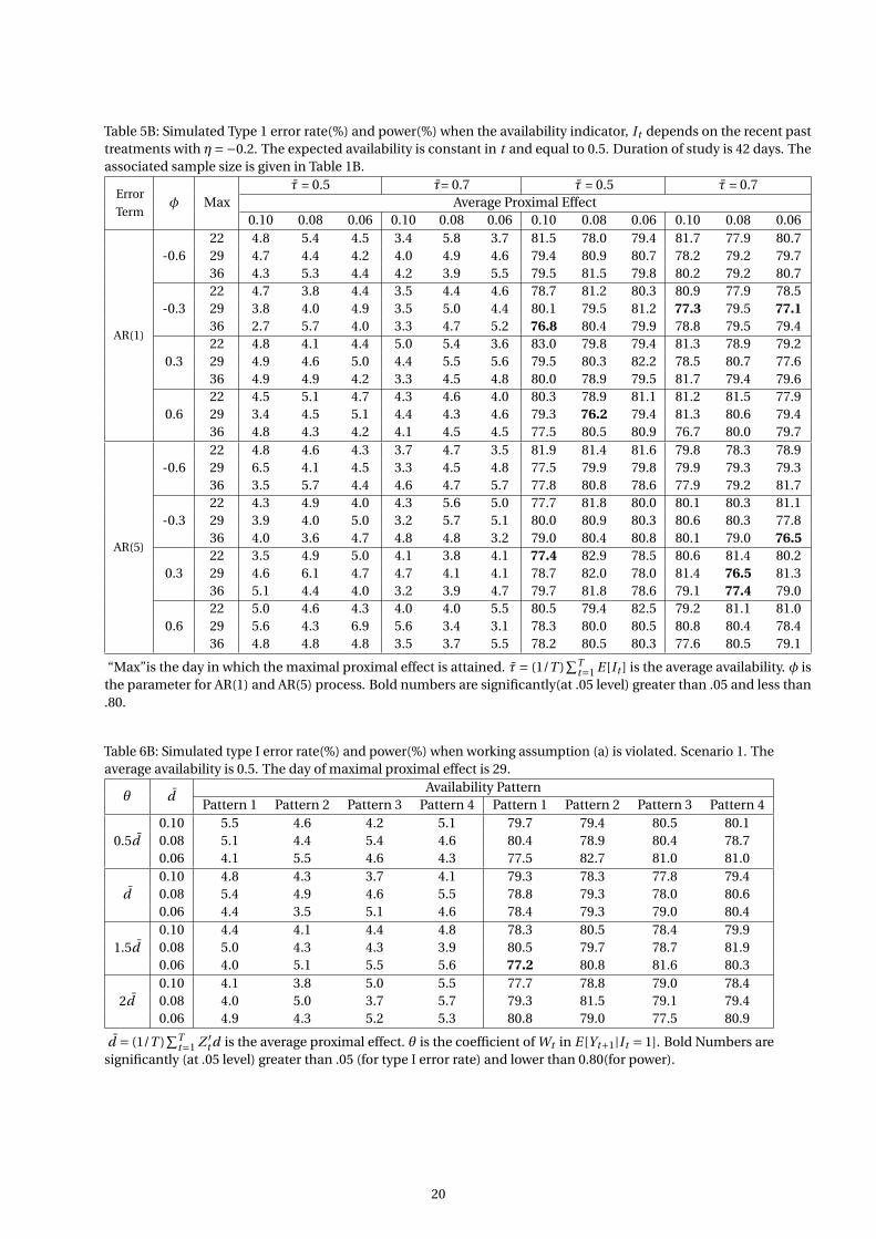
Table 5B: Simulated Type 1 error rate(%) and power(%) when the availability indicator, It depends on the recent pasttreatments with η=−0.2. The expected availability is constant in t and equal to 0.5. Duration of study is 42 days. Theassociated sample size is given in Table 1B.

Error

Termφ Max

τ = 0.5 τ= 0.7 τ = 0.5 τ = 0.7Average Proximal Effect

0.10 0.08 0.06 0.10 0.08 0.06 0.10 0.08 0.06 0.10 0.08 0.06

AR(1)

-0.622 4.8 5.4 4.5 3.4 5.8 3.7 81.5 78.0 79.4 81.7 77.9 80.729 4.7 4.4 4.2 4.0 4.9 4.6 79.4 80.9 80.7 78.2 79.2 79.736 4.3 5.3 4.4 4.2 3.9 5.5 79.5 81.5 79.8 80.2 79.2 80.7

-0.322 4.7 3.8 4.4 3.5 4.4 4.6 78.7 81.2 80.3 80.9 77.9 78.529 3.8 4.0 4.9 3.5 5.0 4.4 80.1 79.5 81.2 77.3 79.5 77.136 2.7 5.7 4.0 3.3 4.7 5.2 76.8 80.4 79.9 78.8 79.5 79.4

0.322 4.8 4.1 4.4 5.0 5.4 3.6 83.0 79.8 79.4 81.3 78.9 79.229 4.9 4.6 5.0 4.4 5.5 5.6 79.5 80.3 82.2 78.5 80.7 77.636 4.9 4.9 4.2 3.3 4.5 4.8 80.0 78.9 79.5 81.7 79.4 79.6

0.622 4.5 5.1 4.7 4.3 4.6 4.0 80.3 78.9 81.1 81.2 81.5 77.929 3.4 4.5 5.1 4.4 4.3 4.6 79.3 76.2 79.4 81.3 80.6 79.436 4.8 4.3 4.2 4.1 4.5 4.5 77.5 80.5 80.9 76.7 80.0 79.7

AR(5)

-0.622 4.8 4.6 4.3 3.7 4.7 3.5 81.9 81.4 81.6 79.8 78.3 78.929 6.5 4.1 4.5 3.3 4.5 4.8 77.5 79.9 79.8 79.9 79.3 79.336 3.5 5.7 4.4 4.6 4.7 5.7 77.8 80.8 78.6 77.9 79.2 81.7

-0.322 4.3 4.9 4.0 4.3 5.6 5.0 77.7 81.8 80.0 80.1 80.3 81.129 3.9 4.0 5.0 3.2 5.7 5.1 80.0 80.9 80.3 80.6 80.3 77.836 4.0 3.6 4.7 4.8 4.8 3.2 79.0 80.4 80.8 80.1 79.0 76.5

0.322 3.5 4.9 5.0 4.1 3.8 4.1 77.4 82.9 78.5 80.6 81.4 80.229 4.6 6.1 4.7 4.7 4.1 4.1 78.7 82.0 78.0 81.4 76.5 81.336 5.1 4.4 4.0 3.2 3.9 4.7 79.7 81.8 78.6 79.1 77.4 79.0

0.622 5.0 4.6 4.3 4.0 4.0 5.5 80.5 79.4 82.5 79.2 81.1 81.029 5.6 4.3 6.9 5.6 3.4 3.1 78.3 80.0 80.5 80.8 80.4 78.436 4.8 4.8 4.8 3.5 3.7 5.5 78.2 80.5 80.3 77.6 80.5 79.1

“Max”is the day in which the maximal proximal effect is attained. τ= (1/T )∑T

t=1 E [It ] is the average availability. φ isthe parameter for AR(1) and AR(5) process. Bold numbers are significantly(at .05 level) greater than .05 and less than.80.

Table 6B: Simulated type I error rate(%) and power(%) when working assumption (a) is violated. Scenario 1. Theaverage availability is 0.5. The day of maximal proximal effect is 29.

θ dAvailability Pattern

Pattern 1 Pattern 2 Pattern 3 Pattern 4 Pattern 1 Pattern 2 Pattern 3 Pattern 4

0.5d0.10 5.5 4.6 4.2 5.1 79.7 79.4 80.5 80.10.08 5.1 4.4 5.4 4.6 80.4 78.9 80.4 78.70.06 4.1 5.5 4.6 4.3 77.5 82.7 81.0 81.0

d0.10 4.8 4.3 3.7 4.1 79.3 78.3 77.8 79.40.08 5.4 4.9 4.6 5.5 78.8 79.3 78.0 80.60.06 4.4 3.5 5.1 4.6 78.4 79.3 79.0 80.4

1.5d0.10 4.4 4.1 4.4 4.8 78.3 80.5 78.4 79.90.08 5.0 4.3 4.3 3.9 80.5 79.7 78.7 81.90.06 4.0 5.1 5.5 5.6 77.2 80.8 81.6 80.3

2d0.10 4.1 3.8 5.0 5.5 77.7 78.8 79.0 78.40.08 4.0 5.0 3.7 5.7 79.3 81.5 79.1 79.40.06 4.9 4.3 5.2 5.3 80.8 79.0 77.5 80.9

d = (1/T )∑T

t=1 Z ′t d is the average proximal effect. θ is the coefficient of Wt in E [Yt+1|It = 1]. Bold Numbers are

significantly (at .05 level) greater than .05 (for type I error rate) and lower than 0.80(for power).

20

Shape 1 Shape 2 Shape 3

2.5

3.0

3.5

4.0

4.5

0 50 100 150 200 0 50 100 150 200 0 50 100 150 200

Time

Response

Figure 4: Conditional expectation of proximal response, E [Yt+1|It = 1]. The horizontal axis is the decision timepoint. The vertical axis is E [Yt+1|It = 1].

Table 7B: Simulated Type 1 error rate(%) and power (%) when working assumption (a) is violated. Scenario 2.The shapes of α(t) = E [Yt+1|It = 1] and patterns of availability are provided in Figure 4 and Figure 1. The averageavailability is 0.5. The day of maximal proximal effect is 29. The associated sample size is given in Table 1B.

Availability Patternα(t ) d Pattern 1 Pattern 2 Pattern 3 Pattern 4 Pattern 1 Pattern 2 Pattern 3 Pattern 4

Shape 10.10 3.6 4.3 4.7 4.5 77.4 80.2 76.2 75.90.08 5.9 3.8 4.1 3.4 79.7 80.1 78.9 80.60.06 4.6 5.7 4.2 6.5 78.7 76.3 78.3 79.9

Shape 20.10 4.8 4.8 4.4 4.1 79.2 79.1 78.5 79.70.08 3.9 5.4 4.8 4.3 77.7 80.4 76.8 80.90.06 5.1 5.5 3.4 4.9 78.3 79.4 79.8 80.2

Shape 30.10 5.1 3.5 4.3 4.4 79.1 79.4 75.6 78.00.08 4.6 5.0 6.2 3.8 78.3 78.1 79.1 78.10.06 4.8 4.4 5.4 4.2 78.0 78.3 79.8 77.7

d = (1/T )∑T

t=1 Z ′t d is the average standardized treatment effect. Bold Numbers are significantly (at .05 level) greater

than .05 (for type I error rate) and lower than 0.80(for power).

Maintained Severely Degraded Slightly Degraded

0.00

0.05

0.10

0.15

0.20

0.00

0.05

0.10

0.15

0.20

0.00

0.05

0.10

0.15

0.20

Ma

x =

15

Ma

x =

22

Ma

x =

29

0 50 100 150 200 0 50 100 150 200 0 50 100 150 200

Time

Pro

xim

al E

ffe

ct

Figure 5: Proximal Main Effects of Treatment, {d(t )}Tt=1: representing maintained, slightly degraded and severely

degraded time-varying treatment effects. The horizontal axis is the decision time point. The vertical axis isthe standardized treatment effect. The "Max" in the title refers to the day of maximal effect. The averagestandardized proximal effect is 0.1 in all plots.

21

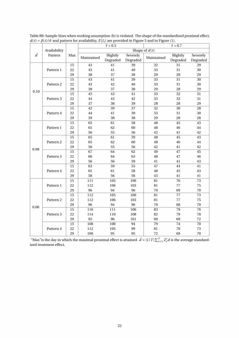
Table 8B: Sample Sizes when working assumption (b) is violated. The shape of the standardized proximal effect,d(t ) =β(t )/σ and pattern for availability, E [It ] are provided in Figure 5 and in Figure (1).

τ = 0.5 τ = 0.7Availability Shape of d(t )

d Pattern MaxMaintained

SlightlyDegraded

SeverelyDegraded

MaintainedSlightly

DegradedSeverely

Degraded

0.10

15 43 41 39 32 31 29Pattern 1 22 43 41 40 33 31 30

29 38 37 38 29 28 2915 43 41 39 33 31 30

Pattern 2 22 43 42 40 33 31 3029 38 37 38 29 28 2915 45 43 41 33 32 31

Pattern 3 22 44 43 42 33 32 3129 37 38 39 28 28 2915 42 39 37 32 30 28

Pattern 4 22 44 41 39 33 31 3029 39 38 38 29 28 28

0.08

15 65 61 58 48 45 43Pattern 1 22 65 62 60 48 46 44

29 56 55 56 42 41 4215 65 61 59 48 45 43

Pattern 2 22 65 62 60 48 46 4429 56 55 56 42 41 4215 67 64 62 49 47 45

Pattern 3 22 66 64 63 48 47 4629 56 56 59 41 41 4315 63 59 55 47 44 41

Pattern 4 22 65 61 58 48 45 4329 58 56 56 43 41 41

0.06

15 111 105 100 81 76 73Pattern 1 22 112 106 103 81 77 75

29 96 94 96 70 69 7015 112 105 100 81 77 73

Pattern 2 22 112 106 103 81 77 7529 96 94 96 70 68 7015 116 111 106 83 79 76

Pattern 3 22 114 110 108 82 79 7829 95 96 101 69 69 7215 108 100 94 79 74 70

Pattern 4 22 112 105 99 81 76 7329 100 95 95 72 69 70

“Max”is the day in which the maximal proximal effect is attained. d = (1/T )∑T

t=1 Z ′t d is the average standard-

ized treatment effect.

22

Table 9B: Simulated Power(%) when working assumption (b) is violated. The shape of the standardizedproximal effect, d(t ) =β(t )/σ and pattern for availability, E [It ] are provided in Figure 5 and in Figure (1). Thecorresponding sample sizes are given in Table 8B.

τ = 0.5 τ = 0.7Availability Shape of d(t )

d Pattern MaxMaintained

SlightlyDegraded

SeverelyDegraded

MaintainedSlightly

DegradedSeverely

Degraded

0.10

15 78.4 78.8 78.6 79.1 80.1 77.6Pattern 1 22 80.4 79.5 81.2 80.0 76.9 77.9

29 80.4 79.2 78.9 77.3 76.8 81.115 78.6 79.9 79.9 80.1 80.4 81.3

Pattern 2 22 78.3 81.2 78.8 79.2 80.8 80.529 77.9 80.8 79.3 78.1 77.7 82.215 81.0 79.7 77.4 77.9 80.9 77.6

Pattern 3 22 78.9 79.1 80.0 79.7 79.4 75.929 80.9 77.5 77.7 80.6 79.2 78.515 79.7 79.5 77.9 79.5 81.7 78.0

Pattern 4 22 78.9 77.9 80.4 82.2 78.9 78.829 77.9 79.7 79.0 78.0 80.2 80.8

0.08

15 80.5 79.5 78.6 80.6 79.2 78.7Pattern 1 22 78.9 78.7 78.8 78.9 80.7 80.3

29 76.6 78.0 78.3 80.9 78.6 80.415 81.0 79.3 78.7 82.0 80.5 80.1

Pattern 2 22 82.4 80.6 80.0 78.0 79.6 79.429 79.2 76.9 81.9 78.3 78.8 79.715 78.2 81.6 80.9 79.1 79.2 77.5

Pattern 3 22 80.9 79.5 78.6 79.2 78.3 81.429 80.4 79.3 77.5 77.9 80.2 82.315 79.4 79.4 78.1 78.6 77.4 78.8

Pattern 4 22 81.3 78.4 78.4 80.6 79.4 80.429 79.9 79.3 79.8 79.5 79.7 81.2

0.06

15 81.2 80.5 79.0 77.8 78.7 79.6Pattern 1 22 80.0 81.7 79.8 80.7 80.5 80.2

29 81.2 78.7 79.2 81.2 79.7 80.115 78.7 77.5 81.4 80.7 81.0 80.7

Pattern 2 22 80.6 81.8 79.2 80.3 81.6 80.229 78.5 80.2 80.0 77.7 78.1 78.015 78.1 80.0 80.9 79.7 79.3 78.8

Pattern 3 22 81.2 80.2 80.0 78.3 82.2 81.129 79.6 81.6 79.8 80.2 81.6 76.915 78.2 79.8 78.9 79.5 77.3 79.2

Pattern 4 22 79.2 81.1 79.4 76.8 79.2 80.429 79.9 78.5 79.8 80.1 78.9 81.8

“Max”is the day in which the maximal proximal effect is attained. d = (1/T )∑T

t=1 Z ′t d is the average standard-

ized treatment effect. Bold numbers are significantly (at .05 level) lower than .80.

23

Table 10B: Simulated Type I error rate(%) and power(%) when working assumption (c) is violated.The trends of σt are provided in Figure 3. The standardized average effect is 0.1. E [It ] = 0.5. Theassociated sample sizes are 41 and 42 when the day of maximal effect is 22 and 29.

Max = 22 Max = 29φ in AR(1) σ1t

σ0tconst. trend 1 trend 2 trend 3 const. trend 1 trend 2 trend 3

0.8 4.1 4.3 3.3 5.4 4.7 4.9 2.8 4.1-0.6 1.0 4.6 5.0 4.0 4.4 4.4 4.8 4.2 4.3

1.2 3.8 4.5 5.2 5.5 4.3 4.1 4.5 3.80.8 5.2 4.7 4.0 3.4 5.4 4.9 6.2 4.5

-0.3 1.0 4.9 4.5 4.5 4.3 5.2 5.1 4.0 3.71.2 5.4 4.6 4.1 3.8 3.7 5.2 4.3 5.00.8 4.8 4.0 4.1 3.9 4.7 5.2 3.7 4.2

0 1.0 5.4 4.0 5.8 3.9 4.1 4.0 5.9 5.71.2 4.4 4.9 5.0 4.6 3.7 4.8 4.4 4.90.8 5.3 4.4 4.7 3.2 4.6 5.4 5.6 4.1

0.3 1.0 5.5 4.0 3.4 3.7 5.0 4.6 4.0 3.61.2 3.8 4.5 4.5 4.8 4.5 5.0 6.2 4.30.8 5.5 3.9 5.3 3.8 3.3 3.5 5.1 4.2

0.6 1.0 4.0 3.7 5.2 5.1 4.8 5.1 5.0 4.71.2 4.5 5.1 4.6 4.9 4.5 4.4 4.7 4.8

0.8 82.8 82.7 83.7 79.9 83.6 80.6 88.7 79.2-0.6 1.0 81.1 79.1 79.9 74.8 77.7 74.3 84.8 70.4

1.2 76.6 76.3 76.3 70.6 77.6 72.0 80.7 70.40.8 83.0 83.0 86.0 80.3 82.7 79.2 87.9 78.0

-0.3 1.0 77.6 81.4 80.7 74.9 79.1 74.5 86.0 73.71.2 78.2 76.9 77.3 73.4 74.4 71.2 81.0 70.70.8 84.6 84.6 82.1 79.0 81.8 81.5 88.0 78.0

0 1.0 80.1 78.6 80.9 73.6 77.7 76.5 86.1 71.81.2 76.0 76.7 77.4 70.6 74.5 69.9 83.4 69.60.8 83.6 79.7 84.6 79.7 82.1 81.7 88.2 75.7

0.3 1.0 81.5 82.4 82.3 73.9 79.5 74.6 85.1 71.51.2 74.8 76.6 78.2 71.1 75.5 71.1 82.5 70.10.8 81.4 83.1 83.5 80.5 83.1 77.1 86.6 76.9

0.6 1.0 80.7 76.4 79.0 74.8 80.4 73.4 84.7 76.81.2 77.0 77.5 77.0 73.5 74.4 72.5 81.6 69.4

φ is the parameter in AR(1) process for {εt }Tt=1. Bold numbers are significantly(at .05 level) greater

than .05 and lower than .80.

Table 11B: Simulated Type I error rate(%) when work-ing assumption (d) is violated. E [It ] = 0.5. The averageeffect is 0.1 and day of maximal effect is 29. N = 42.

Parameters in It γ1

γ2 -0.1 -0.2 -0.3

-0.2 5.7 3.2 3.9η1 =−0.1,η2 =−0.1 -0.5 3.2 4.2 4.9

-0.8 4.2 5.1 5.5-0.2 5.4 3.8 3.9

η1 =−0.2,η2 =−0.1 -0.5 4.4 4.4 4.8-0.8 4.7 4.3 4.6-0.2 4.5 5.0 5.0

η1 =−0.1,η2 =−0.2 -0.5 4.9 3.8 6.0-0.8 4.7 4.8 4.8

η1,η2 are parameters in generating It . γ1, γ2 are coef-ficients in the model of Yt+1. Bold Numbers are signifi-cantly (at .05 level) greater than .05.

24

Table 12B: Degradation in power when average proximal effect is underesti-mated. Day of maximal effect is 29 and the average availability is 0.5.

d in SampleSize Formula

True dAvailability Pattern

Pattern 1 Pattern 2 Pattern 3 Pattern 4

0.10 (N = 42)

0.098 76.2 78.9 77.6 78.60.096 75.1 74.6 78.8 74.00.094 73.7 70.7 75.4 73.40.092 71.5 71.6 73.2 71.60.090 68.9 68.4 69.6 67.30.088 65.4 65.6 66.1 65.70.086 66.4 67.9 65.2 66.70.084 62.3 63.4 63.0 59.60.082 60.0 60.2 60.5 58.20.080 58.9 59.8 57.8 61.4

0.08(N = 64)

0.078 78.2 80.2 76.8 75.80.076 77.3 76.7 76.2 75.40.074 73.1 72.2 71.2 71.40.072 70.7 71.0 69.4 68.20.070 68.2 66.0 65.2 66.10.068 65.5 64.3 64.6 65.70.066 62.8 62.3 61.8 59.40.064 61.9 58.5 59.5 62.10.062 53.9 52.6 57.0 56.90.060 54.6 51.1 54.8 53.4

0.06(N = 109)

0.058 75.6 76.9 74.0 78.10.056 73.9 73.1 73.1 72.70.054 68.6 71.1 69.3 68.50.052 65.4 69.4 63.6 66.80.050 61.0 62.8 64.1 63.20.048 57.4 58.6 56.4 56.10.046 53.6 53.4 52.9 54.80.044 52.0 48.9 50.1 53.00.042 45.7 43.9 44.9 46.40.040 40.4 42.2 42.3 42.7

Table 13B: Degradation in Power when average availability is underestimated. The day ofmaximal treatment effect is attained at day 29 and the average proximal main effect is 0.1.

(1/T )∑T

t=1τt in True Availability PatternSample Size Formula (1/T )

∑Tt=1τt Pattern 1 Pattern 2 Pattern 3 Pattern 4

0.5 (N = 42)

0.048 76.4 81.7 76.0 78.20.046 73.9 75.5 73.6 75.80.044 70.6 72.1 71.0 71.70.042 70.8 70.6 74.2 70.30.040 70.3 69.2 65.7 68.60.038 66.0 66.8 67.8 67.00.036 64.0 62.5 62.4 62.90.034 60.8 61.3 59.4 63.90.032 56.4 59.2 54.7 59.80.030 51.4 53.1 51.9 54.5

0.7 (N = 32)

0.068 79.5 76.1 79.1 75.00.066 77.3 75.7 74.0 76.40.064 74.5 74.7 73.5 77.10.062 73.2 73.0 75.1 72.50.060 69.8 70.5 73.5 72.50.058 71.0 69.6 71.3 67.30.056 68.8 70.3 66.6 64.00.054 68.1 65.8 65.3 68.60.052 62.4 64.9 65.6 62.90.050 60.6 63.3 62.8 61.4

25

AcknowledgmentThis research was supported by NIH grants P50DA010075, R01HL12544001 and grant U54EB020404 awardedby the National Institute of Biomedical Imaging and Bioengineering (NIBIB) through funds provided by thetrans-NIH Big Data to Knowledge (BD2K) initiative (www.bd2k.nih.gov).

References

1. A. CUCCIARE, M., R. WEINGARDT, K., J. GREENE, C., AND HOFFMAN, J. Current trends in using internet andmobile technology to support the treatment of substance use disorders. Current Drug Abuse Reviews 5, 3(2012), 172–177.

2. ALESSI, S. M., AND PETRY, N. M. A randomized study of cellphone technology to reinforce alcohol abstinencein the natural environment. Addiction 108, 5 (2013), 900–909.

3. BOX, G. E., P.HUNTER, J. S., AND HUNTER, W. G. Statistics for experimenters : an introduction to design,data analysis, and model building. Wiley series in probability and mathematical statistics, 1978.

4. BOYER, E., FLETCHER, R., FAY, R., SMELSON, D., ZIEDONIS, D., AND PICARD, R. Preliminary efforts directedtoward the detection of craving of illicit substances: The iheal project. Journal of Medical Toxicology 8, 1(2012), 5–9.

5. BUMAN, M., HEKLER, E., FLOEGEL, T., FLOREZ PREGONERO, A., G., M., AND RILEY, K. Step validation of thejawbone up band in normal, overweight, and obese adults. In Proceedings of the American Medical Societyfor Sports Medicine. (2014).

6. CHAKRABORTY, B., COLLINS, L. M., STRECHER, V. J., AND MURPHY, S. A. Developing multicomponentinterventions using fractional factorial designs. Statistics in Medicine 28, 21 (2009), 2687–2708.

7. COHEN, J. Statistical Power Analysis for the Behavioral Sciences(2nd), 2nd ed. Routledge, July 1 1988.8. FREE, C., PHILLIPS, G., GALLI, L., WATSON, L., FELIX, L., EDWARDS, P., PATEL, V., AND HAINES, A. The effec-

tiveness of mobile-health technology-based health behaviour change or disease management interventionsfor health care consumers: A systematic review. PLoS Med 10, 1 (01 2013), e1001362.

9. GUSTAFSON, D., FM, M., M, C., AND ET AL. A smartphone application to support recovery from alcoholism:A randomized clinical trial. JAMA Psychiatry 71, 5 (2014), 566–572.

10. HOTELLING, H. The generalization of student’s ratio. Ann. Math. Statist. 2, 3 (08 1931), 360–378.11. KAPLAN, R. M., AND STONE, A. A. Bringing the laboratory and clinic to the community: Mobile technologies

for health promotion and disease prevention. Annual Review of Psychology 64, 1 (2013), 471–498. PMID:22994919.

12. KING, A. C., CASTRO, C. M., BUMAN, M. P., HEKLER, E. B., URIZAR, GUIDO G., J., AND AHN, D. K. Behavioralimpacts of sequentially versus simultaneously delivered dietary plus physical activity interventions: thecalm trial. Annals of Behavioral Medicine 46, 2 (2013), 157–168.

13. KUMAR, S., NILSEN, W., PAVEL, M., AND SRIVASTAVA, M. Mobile health: Revolutionizing healthcare throughtransdisciplinary research. Computer 46, 1 (2013), 28–35.

14. LEWIS, M. A., UHRIG, J. D., BANN, C. M., HARRIS, J. L., FURBERG, R. D., COOMES, C., AND KUHNS, L. M.Tailored text messaging intervention for hiv adherence: a proof-of-concept study. Health psychology :official journal of the Division of Health Psychology, American Psychological Association 32, 3 (March 2013),248—253.

15. LI, P., AND REDDEN, D. T. Small sample performance of bias-corrected sandwich estimators for cluster-randomized trials with binary outcomes. Statistics in Medicine 34, 2 (2015), 281–296.

16. LIANG, K.-Y., AND ZEGER, S. L. Longitudinal data analysis using generalized linear models. Biometrika 73, 1(1986), 13–22.

17. MANCL, L. A., AND DEROUEN, T. A. A covariance estimator for gee with improved small-sample properties.Biometrics 57, 1 (2001), 126–134.

18. MARSCH, L. A. Leveraging technology to enhance addiction treatment and recovery. Journal of AddictiveDiseases 31, 3 (2012), 313–318. PMID: 22873192.

19. MUESSIG, E. K., PIKE, C. E., LEGRAND, S., AND HIGHTOW-WEIDMAN, B. L. Mobile phone applications forthe care and prevention of hiv and other sexually transmitted diseases: A review. J Med Internet Res 15, 1(Jan 2013), e1.

20. NILSEN, W., KUMAR, S., SHAR, A., VAROQUIERS, C., WILEY, T., RILEY, W. T., PAVEL, M., AND ATIENZA, A. A.Advancing the science of mhealth. Journal of Health Communication 17, sup1 (2012), 5–10.

26

21. QUANBECK, A., GUSTAFSON, D., MARSCH, L., MCTAVISH, F., BROWN, R., MARES, M.-L., JOHNSON, R.,GLASS, J., ATWOOD, A., AND MCDOWELL, H. Integrating addiction treatment into primary care using mobilehealth technology: protocol for an implementation research study. Implementation Science 9, 1 (2014), 65.

22. ROBINS, J. A new approach to causal inference in mortality studies with a sustained exposure period—application to control of the healthy worker survivor effect. Mathematical Modelling 7, 9–12 (1986), 1393 –1512.

23. ROBINS, J. Addendum to “a new approach to causal inference in mortality studies with a sustained exposureperiod—application to control of the healthy worker survivor effect”. Computers and Mathematics withApplications 14, 9–12 (1987), 923 – 945.

24. ROBINS, J. M. Optimal structural nested models for optimal sequential decisions. In Proceedings of theSecond Seattle Symposium on Biostatistics (New York, 2004), D. Y. Lin and P. Heagerty, Eds., Springer, pp. 189–326.

25. RUBIN, D. B. Bayesian inference for causal effects: The role of randomization. Ann. Statist. 6, 1 (01 1978),34–58.

26. SPRUIJT-METZ, D., AND NILSEN, W. Dynamic models of behavior for just-in-time adaptive interventions.Pervasive Computing, IEEE 13, 3 (July 2014), 13–17.

27. TU, X. M., KOWALSKI, J., ZHANG, J., LYNCH, K. G., AND CRITS-CHRISTOPH, P. Power analyses for longitudinaltrials and other clustered designs. Statistics in Medicine 23, 18 (2004), 2799–2815.

28. WANG, L., ROTNITZKY, A., LIN, X., MILLIKAN, R. E., AND THALL, P. F. Evaluation of viable dynamic treatmentregimes in a sequentially randomized trial of advanced prostate cancer. Journal of the American StatisticalAssociation 107, 498 (2012), 493–508.

27