Embed Size (px)
Citation preview

Microarray Analysis with R/Bioconductor
Jiangwen Zhang, Ph.D.
Outline
o Overview of R and Bioconductor n Installation, updating and self learning
resources o Basic commands in R o Using Bioconductor for various steps of
microarray analysis (both 1 & 2 channels)

A quick overview
o R & Bioconductor n http://www.r-project.org n A statistical environment which implements a
dialect of the S language that was developed at AT&T Bell lab
n Open source, cross platform n Mainly command-line driven n Current release: 2.9 n http://www.bioconductor.org n Open source software packages written in R for
bioinformatics application n Mainly for microarray analysis at the moment n Current release: 2.4
o Advantages n Cross platform
o Linux, windows and MacOS n Comprehensive and centralized
o Analyzes both Affymetrix and two color spotted microarrays, and covers various stages of data analysis in a single environment
n Cutting edge analysis methods o New methods/functions can easily be incorporated and
implemented n Quality check of data analysis methods
o Algorithms and methods have undergone evaluation by statisticians and computer scientists before launch. And in many cases there are also literature references
n Good documentations o Comprehensive manuals, documentations, course materials,
course notes and discussion group are available n A good chance to learn statistics and programming
o Limitations n Not easy to learn
o Require a substantial effort to learn statistics and programming skills before one can do a meaningful data analysis
n Not intuitive o Mainly command-line based analysis o There are limited wrapper functions and GUIs for certain
basic functions
How to download, install and update the basic packages
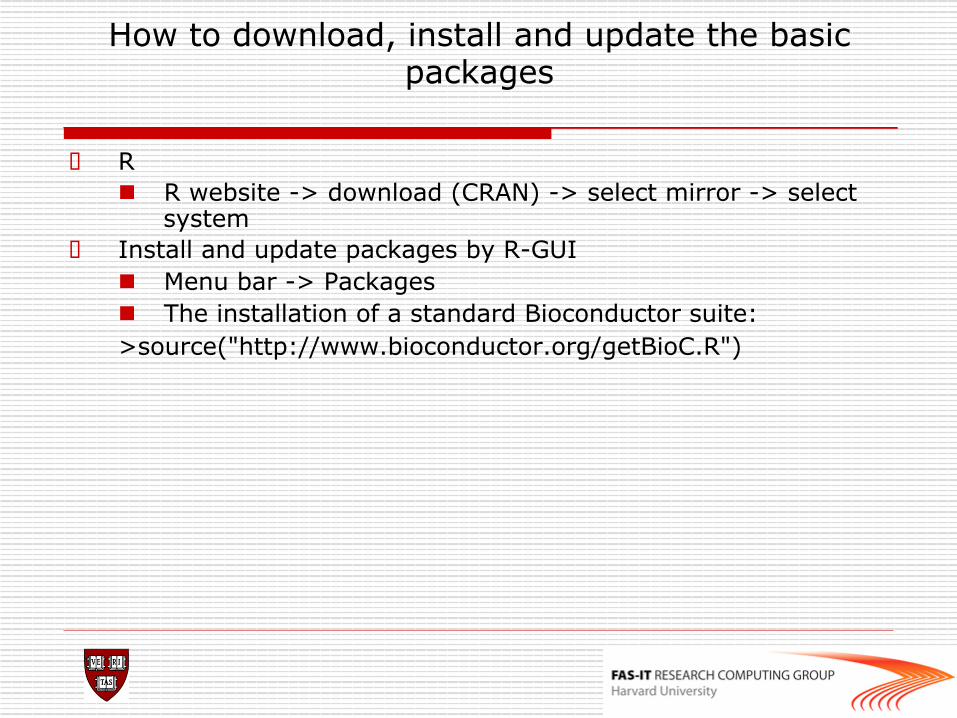
o R n R website -> download (CRAN) -> select mirror -> select
system o Install and update packages by R-GUI
n Menu bar -> Packages n The installation of a standard Bioconductor suite: >source("http://www.bioconductor.org/getBioC.R")
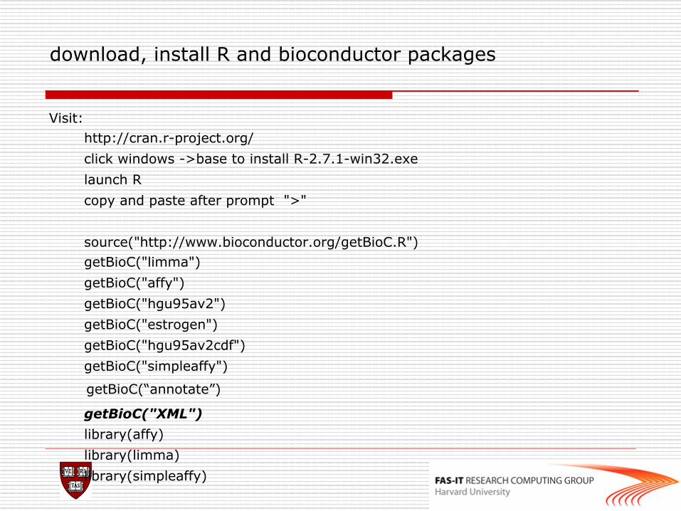
download, install R and bioconductor packages
Visit: http://cran.r-project.org/ click windows ->base to install R-2.7.1-win32.exe launch R copy and paste after prompt ">" source("http://www.bioconductor.org/getBioC.R") getBioC("limma") getBioC("affy") getBioC("hgu95av2") getBioC("estrogen") getBioC("hgu95av2cdf") getBioC("simpleaffy")
getBioC(“annotate”)
getBioC("XML") library(affy) library(limma) library(simpleaffy)
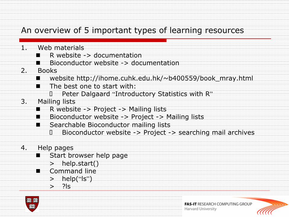
An overview of 5 important types of learning resources
1. Web materials n R website -> documentation n Bioconductor website -> documentation
2. Books n website http://ihome.cuhk.edu.hk/~b400559/book_mray.html n The best one to start with:
o Peter Dalgaard “Introductory Statistics with R” 3. Mailing lists
n R website -> Project -> Mailing lists n Bioconductor website -> Project -> Mailing lists n Searchable Bioconductor mailing lists
o Bioconductor website -> Project -> searching mail archives 4. Help pages
n Start browser help page > help.start()
n Command line > help(“ls”) > ?ls
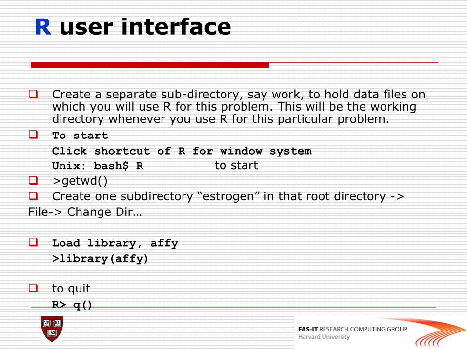
R user interface
q Create a separate sub-directory, say work, to hold data files on which you will use R for this problem. This will be the working directory whenever you use R for this particular problem.
q To start Click shortcut of R for window system Unix: bash$ R to start
q >getwd() q Create one subdirectory “estrogen” in that root directory -> File-> Change Dir…
q Load library, affy
>library(affy)
q to quit R> q()
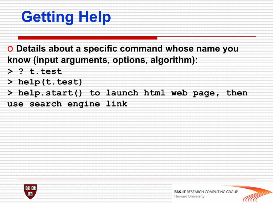
Getting Help
o Details about a specific command whose name you know (input arguments, options, algorithm): > ? t.test > help(t.test) > help.start() to launch html web page, then use search engine link
• Simple manipulations numbers and vectors • Factors, Arrays and matrices • Lists and data frames • Reading data from files • Probability distributions • Loops and conditional execution • Writing your own functions • Statistical models in R • Graphics • Packages
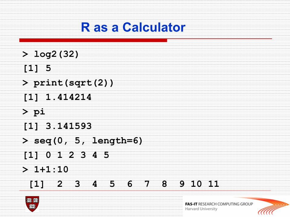
R as a Calculator
> log2(32) [1] 5
> print(sqrt(2))
[1] 1.414214
> pi
[1] 3.141593
> seq(0, 5, length=6)
[1] 0 1 2 3 4 5
> 1+1:10
[1] 2 3 4 5 6 7 8 9 10 11
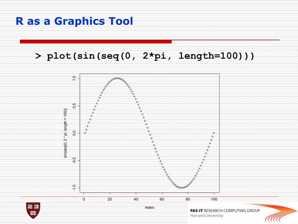
R as a Graphics Tool
> plot(sin(seq(0, 2*pi, length=100)))
0 20 40 60 80 100
-1.0
-0.5
0.0
0.5
1.0
Index
sin(
seq(
0, 2
* pi
, len
gth
= 10
0))
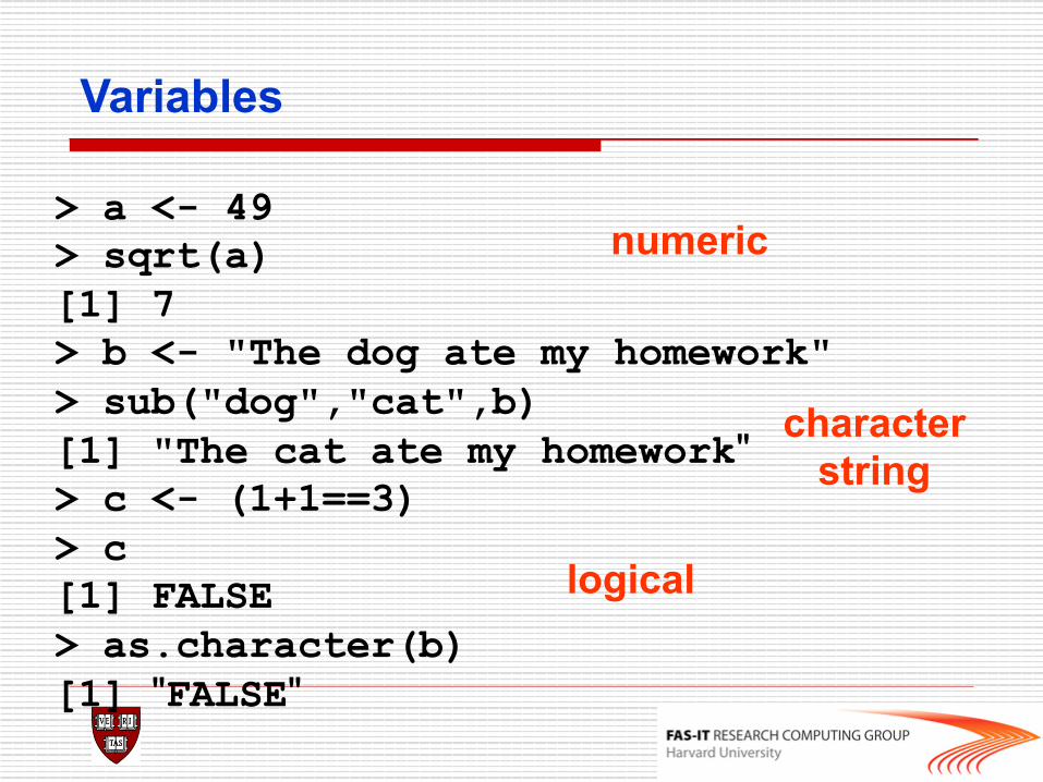
> a <- 49 > sqrt(a) [1] 7 > b <- "The dog ate my homework" > sub("dog","cat",b) [1] "The cat ate my homework" > c <- (1+1==3) > c [1] FALSE > as.character(b) [1] "FALSE"
numeric
character string
logical
Variables
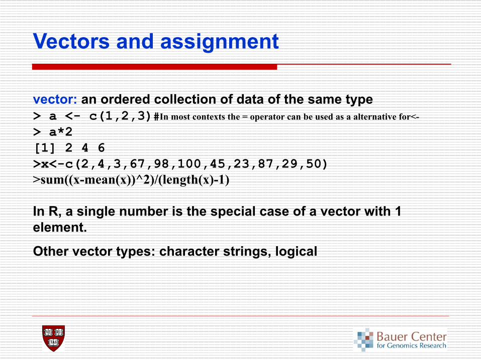
Vectors and assignment
vector: an ordered collection of data of the same type > a <- c(1,2,3)#In most contexts the = operator can be used as a alternative for<-
> a*2 [1] 2 4 6 >x<-c(2,4,3,67,98,100,45,23,87,29,50) >sum((x-mean(x))^2)/(length(x)-1) In R, a single number is the special case of a vector with 1 element.
Other vector types: character strings, logical
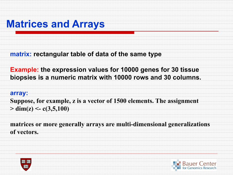
Matrices and Arrays
matrix: rectangular table of data of the same type Example: the expression values for 10000 genes for 30 tissue biopsies is a numeric matrix with 10000 rows and 30 columns. array: Suppose, for example, z is a vector of 1500 elements. The assignment > dim(z) <- c(3,5,100) matrices or more generally arrays are multi-dimensional generalizations of vectors.
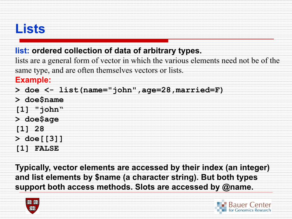
Lists list: ordered collection of data of arbitrary types. lists are a general form of vector in which the various elements need not be of the same type, and are often themselves vectors or lists. Example: > doe <- list(name="john",age=28,married=F) > doe$name [1] "john“ > doe$age [1] 28 > doe[[3]] [1] FALSE Typically, vector elements are accessed by their index (an integer) and list elements by $name (a character string). But both types support both access methods. Slots are accessed by @name.
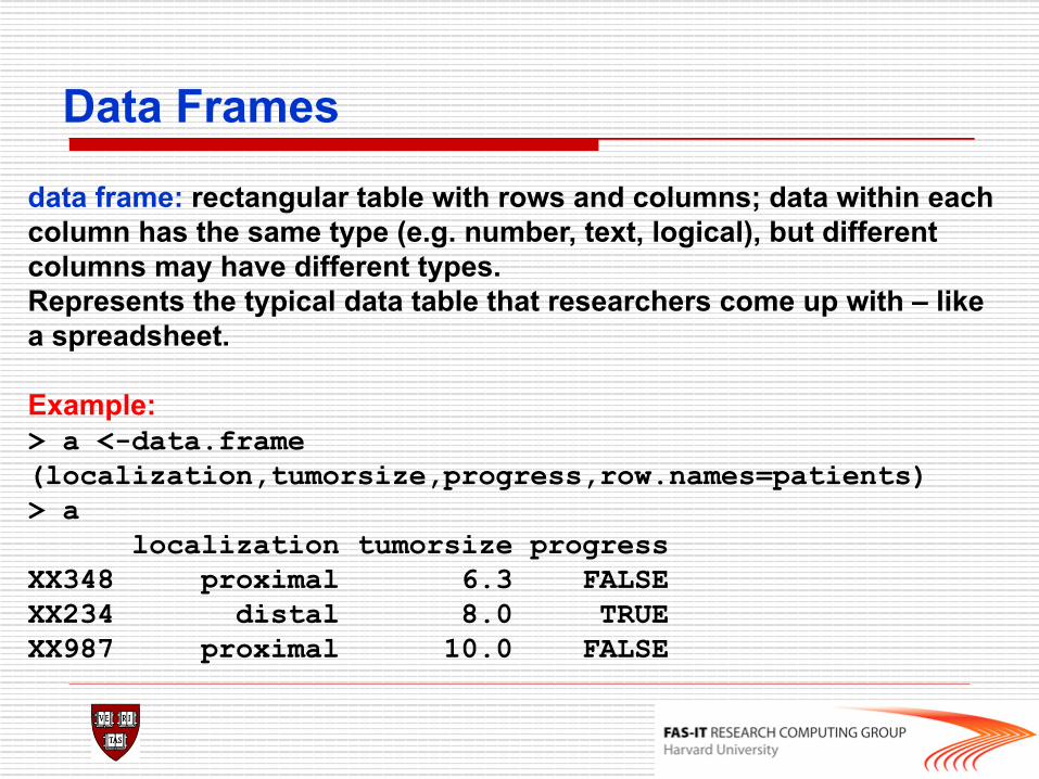
Data Frames
data frame: rectangular table with rows and columns; data within each column has the same type (e.g. number, text, logical), but different columns may have different types. Represents the typical data table that researchers come up with – like a spreadsheet. Example: > a <-data.frame(localization,tumorsize,progress,row.names=patients) > a localization tumorsize progress XX348 proximal 6.3 FALSE XX234 distal 8.0 TRUE XX987 proximal 10.0 FALSE
Reading data from files
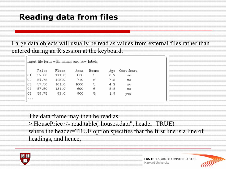
Large data objects will usually be read as values from external files rather than entered during an R session at the keyboard.
The data frame may then be read as > HousePrice <- read.table("houses.data", header=TRUE) where the header=TRUE option specifies that the first line is a line of headings, and hence,
Importing and Exporting Data
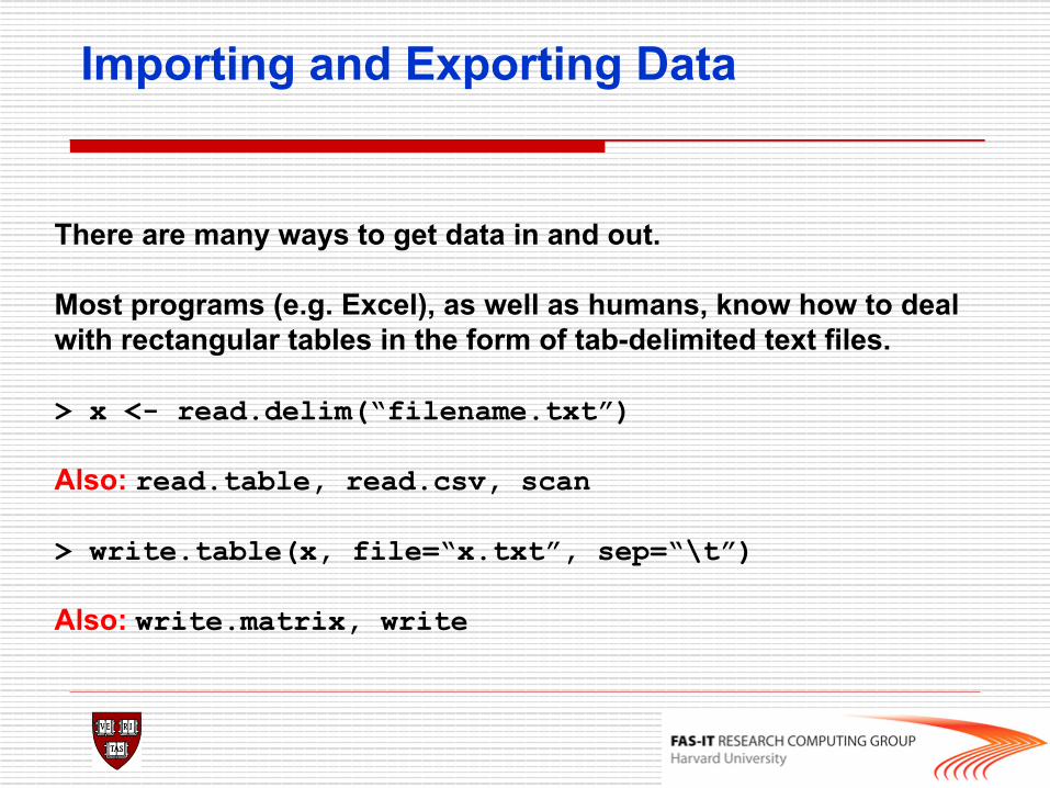
There are many ways to get data in and out. Most programs (e.g. Excel), as well as humans, know how to deal with rectangular tables in the form of tab-delimited text files. > x <- read.delim(“filename.txt”) Also: read.table, read.csv, scan > write.table(x, file=“x.txt”, sep=“\t”) Also: write.matrix, write
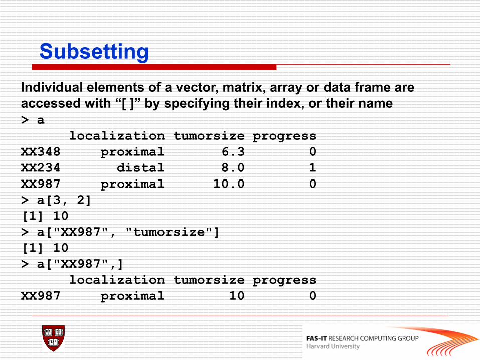
Subsetting Individual elements of a vector, matrix, array or data frame are accessed with “[ ]” by specifying their index, or their name > a localization tumorsize progress XX348 proximal 6.3 0 XX234 distal 8.0 1 XX987 proximal 10.0 0 > a[3, 2] [1] 10 > a["XX987", "tumorsize"] [1] 10 > a["XX987",] localization tumorsize progress XX987 proximal 10 0
Loops
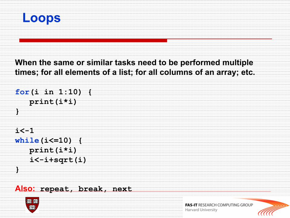
When the same or similar tasks need to be performed multiple times; for all elements of a list; for all columns of an array; etc. for(i in 1:10) { print(i*i) } i<-1 while(i<=10) { print(i*i) i<-i+sqrt(i) } Also: repeat, break, next
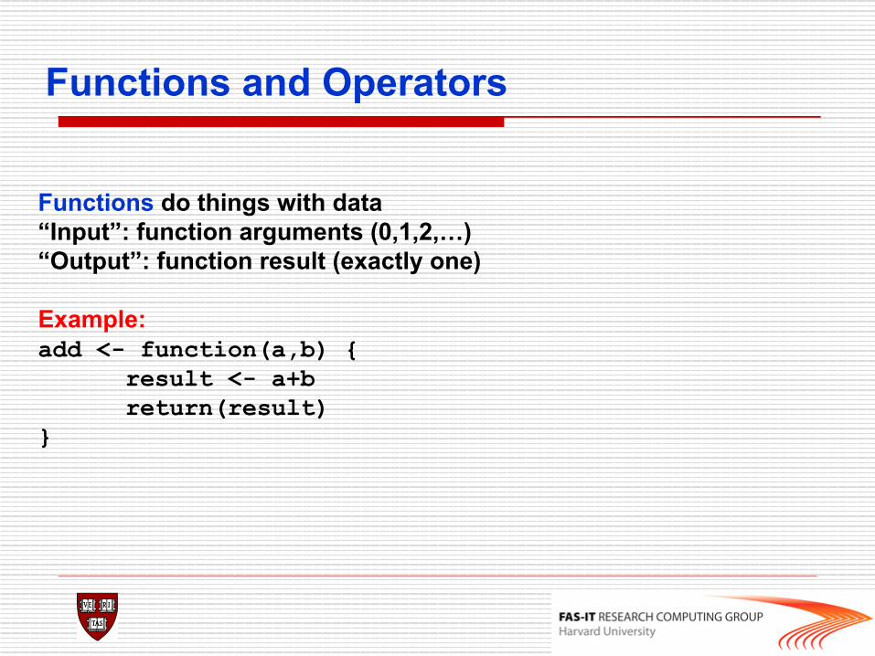
Functions and Operators
Functions do things with data “Input”: function arguments (0,1,2,…) “Output”: function result (exactly one) Example: add <- function(a,b) {
result <- a+b return(result) }
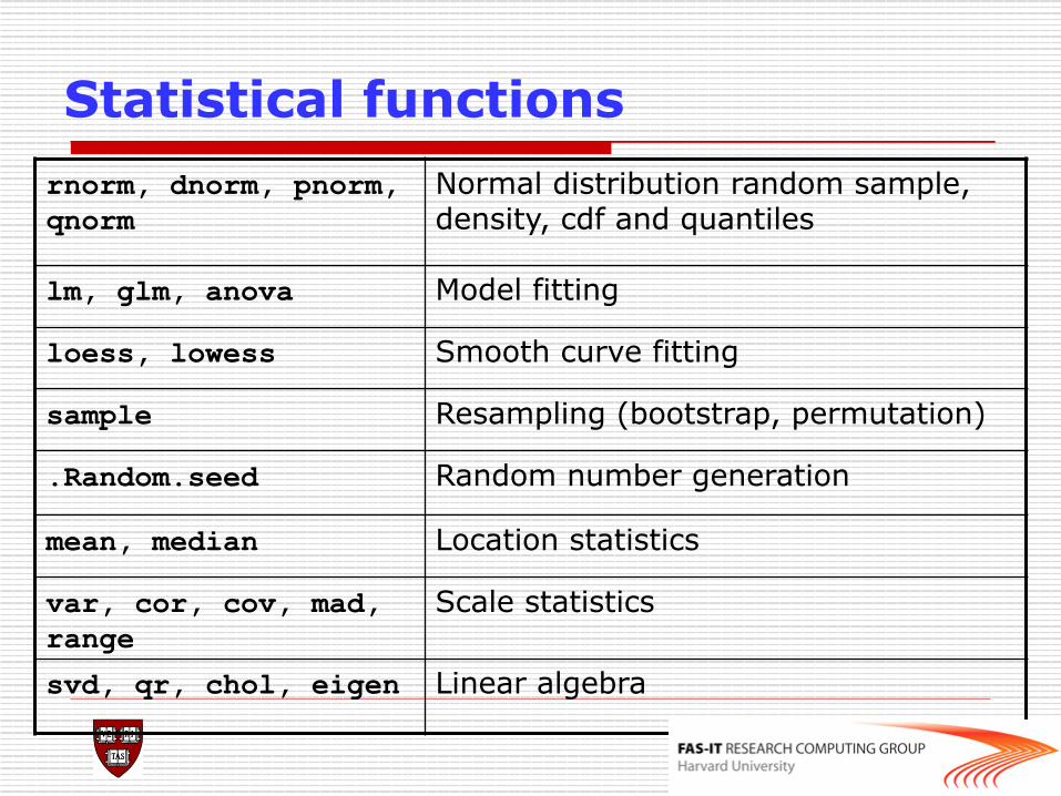
Statistical functions rnorm, dnorm, pnorm, qnorm
Normal distribution random sample, density, cdf and quantiles
lm, glm, anova Model fitting
loess, lowess Smooth curve fitting
sample Resampling (bootstrap, permutation)
.Random.seed Random number generation
mean, median Location statistics
var, cor, cov, mad, range
Scale statistics
svd, qr, chol, eigen Linear algebra
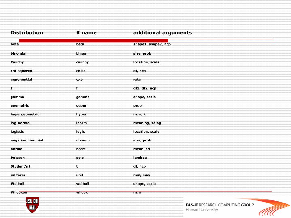
Distribution R name additional arguments
beta beta shape1, shape2, ncp
binomial binom size, prob
Cauchy cauchy location, scale
chi-squared chisq df, ncp
exponential exp rate
F f df1, df2, ncp
gamma gamma shape, scale
geometric geom prob
hypergeometric hyper m, n, k
log-normal lnorm meanlog, sdlog
logistic logis location, scale
negative binomial nbinom size, prob
normal norm mean, sd
Poisson pois lambda
Student's t t df, ncp
uniform unif min, max
Weibull weibull shape, scale
Wilcoxon wilcox m, n
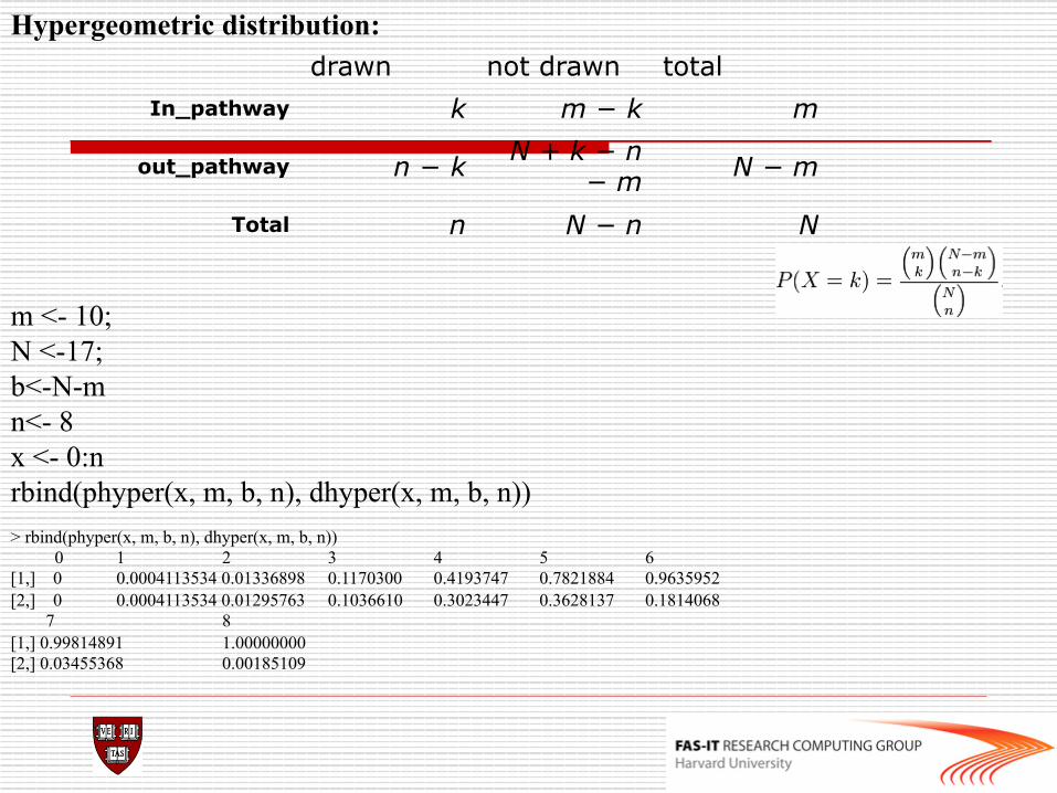
m <- 10; N <-17; b<-N-m n<- 8 x <- 0:n rbind(phyper(x, m, b, n), dhyper(x, m, b, n))
drawn not drawn total In_pathway k m − k m
out_pathway n − k N + k − n − m N − m
Total n N − n N
> rbind(phyper(x, m, b, n), dhyper(x, m, b, n)) 0 1 2 3 4 5 6 [1,] 0 0.0004113534 0.01336898 0.1170300 0.4193747 0.7821884 0.9635952 [2,] 0 0.0004113534 0.01295763 0.1036610 0.3023447 0.3628137 0.1814068 7 8 [1,] 0.99814891 1.00000000 [2,] 0.03455368 0.00185109
Hypergeometric distribution:
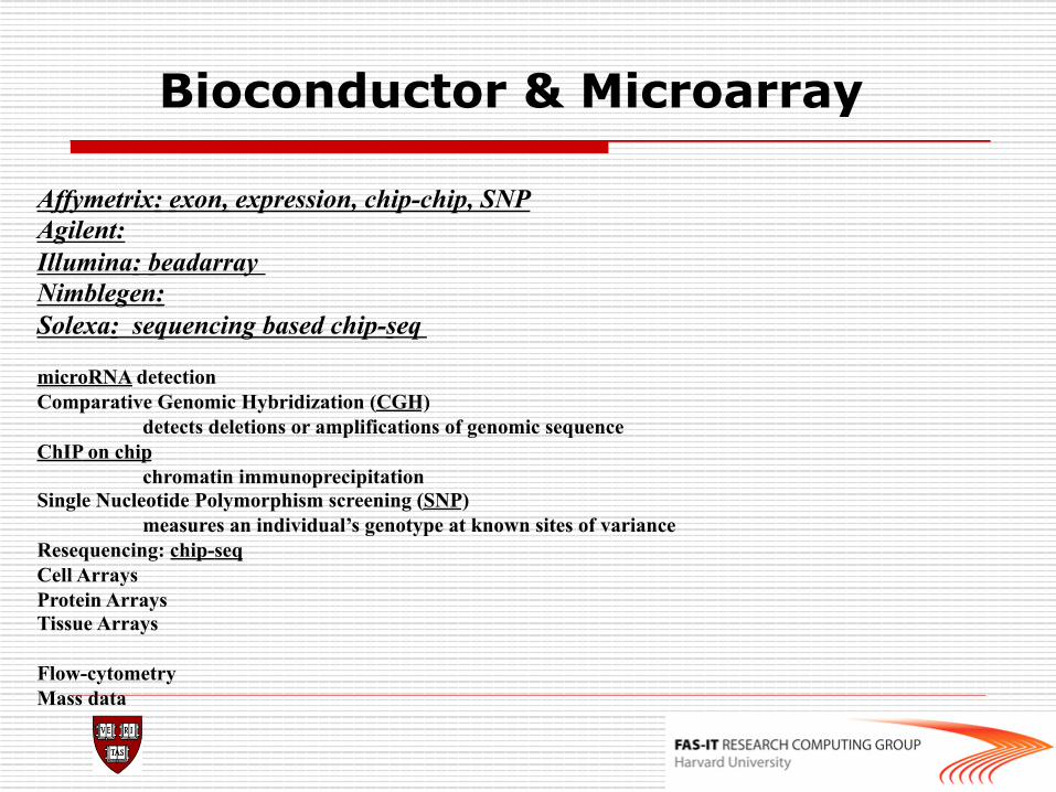
Bioconductor & Microarray Affymetrix: exon, expression, chip-chip, SNP
Agilent: Illumina: beadarray Nimblegen: Solexa: sequencing based chip-seq microRNA detection Comparative Genomic Hybridization (CGH)
detects deletions or amplifications of genomic sequence ChIP on chip
chromatin immunoprecipitation Single Nucleotide Polymorphism screening (SNP)
measures an individual’s genotype at known sites of variance Resequencing: chip-seq Cell Arrays Protein Arrays Tissue Arrays Flow-cytometry Mass data
Challenges in Genomics
•Diverse biological data types: Genotype, Copy Number, Transcription, Methylation,… •Diverse technologies to measure the above: Affymetrix, Nimblegen,… •Integration of multiple and diverse data structures •Large datasets Functional genomics, gene regulation network, signaling pathway, motif identification
Aims of Bioconductor
o Provide access to powerful statistical and graphical methods for the analysis of genomic data.
o Facilitate the integration of biological metadata (GenBank, GO, LocusLink, PubMed) in the analysis of experimental data.
o Allow the rapid development of extensible, interoperable, and scalable software.
o Promote high-quality documentation and reproducible research.
o Provide training in computational and statistical methods.
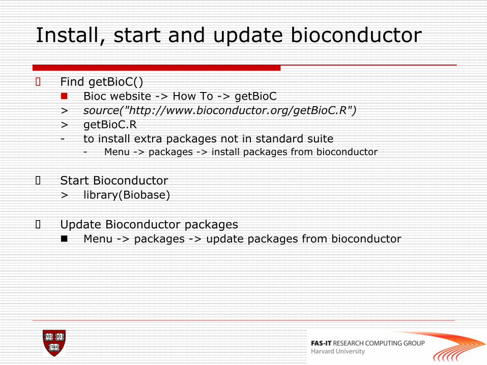
Install, start and update bioconductor
o Find getBioC() n Bioc website -> How To -> getBioC > source("http://www.bioconductor.org/getBioC.R") > getBioC.R - to install extra packages not in standard suite
- Menu -> packages -> install packages from bioconductor
o Start Bioconductor > library(Biobase)
o Update Bioconductor packages n Menu -> packages -> update packages from bioconductor
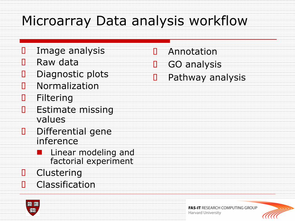
Microarray Data analysis workflow
o Image analysis o Raw data o Diagnostic plots o Normalization o Filtering o Estimate missing
values o Differential gene
inference n Linear modeling and
factorial experiment o Clustering o Classification
o Annotation o GO analysis o Pathway analysis
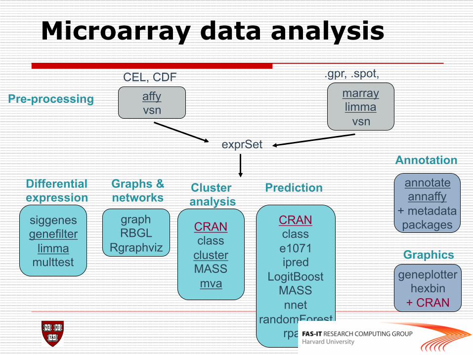
Microarray data analysis CEL, CDF
affy vsn
.gpr, .spot,
Pre-processing
exprSet
graph RBGL
Rgraphviz
siggenes genefilter
limma multtest
annotate annaffy
+ metadata packages CRAN
class cluster MASS mva
geneplotter hexbin
+ CRAN
marray limma
vsn
Differential expression
Graphs & networks
Cluster analysis
Annotation
CRAN class e1071 ipred
LogitBoost MASS nnet
randomForest rpart
Prediction
Graphics
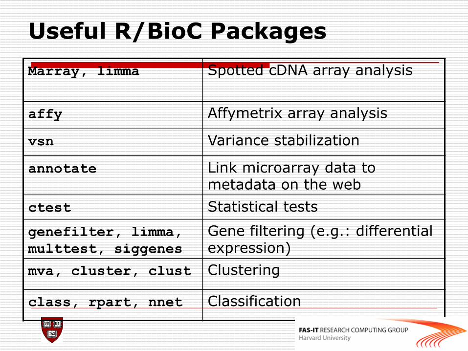
Useful R/BioC Packages Marray, limma Spotted cDNA array analysis
affy Affymetrix array analysis
vsn Variance stabilization
annotate Link microarray data to metadata on the web
ctest Statistical tests
genefilter, limma, multtest, siggenes
Gene filtering (e.g.: differential expression)
mva, cluster, clust Clustering
class, rpart, nnet Classification
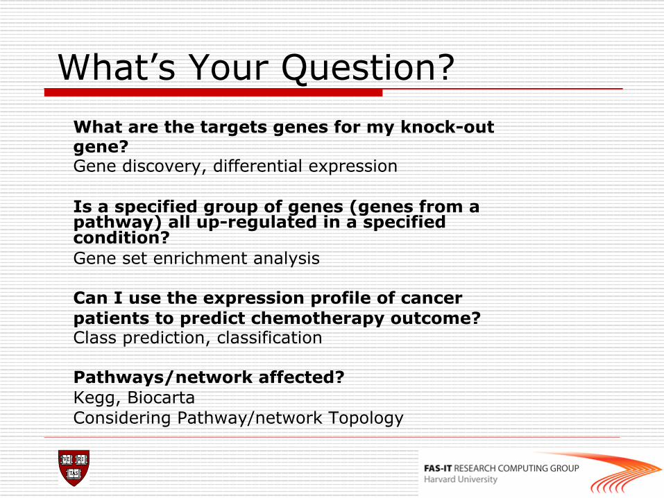
What’s Your Question? What are the targets genes for my knock-out gene? Gene discovery, differential expression Is a specified group of genes (genes from a pathway) all up-regulated in a specified condition? Gene set enrichment analysis Can I use the expression profile of cancer patients to predict chemotherapy outcome? Class prediction, classification Pathways/network affected? Kegg, Biocarta Considering Pathway/network Topology
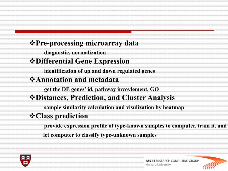
v Pre-processing microarray data diagnostic, normalization v Differential Gene Expression identification of up and down regulated genes v Annotation and metadata get the DE genes’ id, pathway invovlement, GO v Distances, Prediction, and Cluster Analysis sample similarity calculation and visulization by heatmap v Class prediction provide expression profile of type-known samples to computer, train it, and let computer to classify type-unknown samples
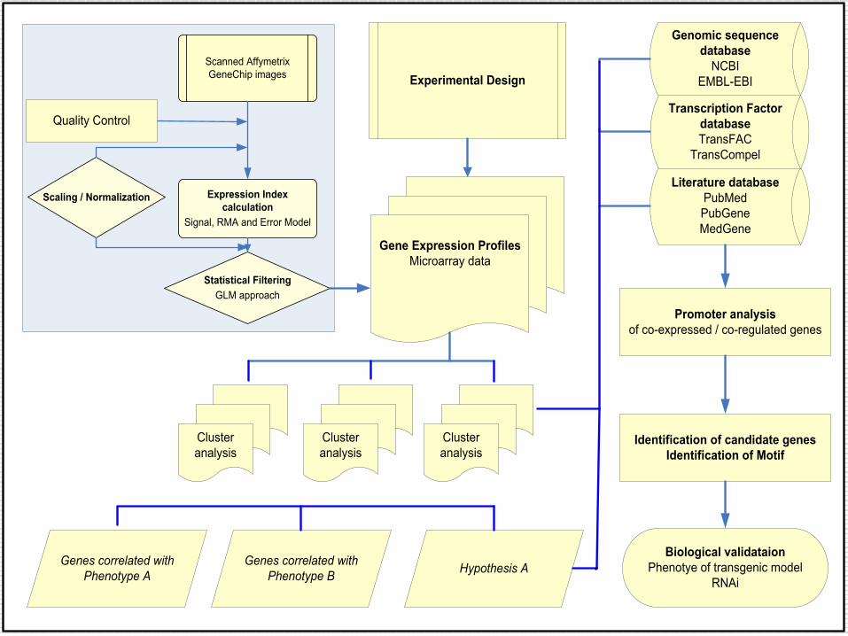
Experimental Design
Cluster analysis
Cluster analysis
Cluster analysis
Genes correlated with Phenotype A
Biological validataionPhenotye of transgenic model
RNAi
Promoter analysis of co-expressed / co-regulated genes
Expression Index calculation
Signal, RMA and Error Model
Scaling / Normalization
Statistical FilteringGLM approach
Scanned Affymetrix GeneChip images
Gene Expression ProfilesMicroarray data
Genomic sequence database
NCBIEMBL-EBI
Literature databasePubMedPubGeneMedGene
Transcription Factor databaseTransFAC
TransCompel
Genes correlated with Phenotype B Hypothesis A
Identification of candidate genesIdentification of Motif
Quality Control
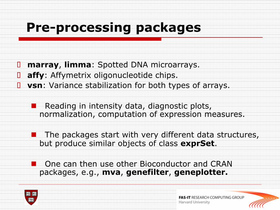
Pre-processing packages
o marray, limma: Spotted DNA microarrays. o affy: Affymetrix oligonucleotide chips. o vsn: Variance stabilization for both types of arrays.
n Reading in intensity data, diagnostic plots, normalization, computation of expression measures.
n The packages start with very different data structures, but produce similar objects of class exprSet.
n One can then use other Bioconductor and CRAN packages, e.g., mva, genefilter, geneplotter.
LIMMA and LIMMA GUI
o LIMMA is another library to perform basic 2 channels analysis, linear modeling for both single channel and 2 channel
o There is a nice GUI for LIMMA o library(limma) o library(limmaGUI)
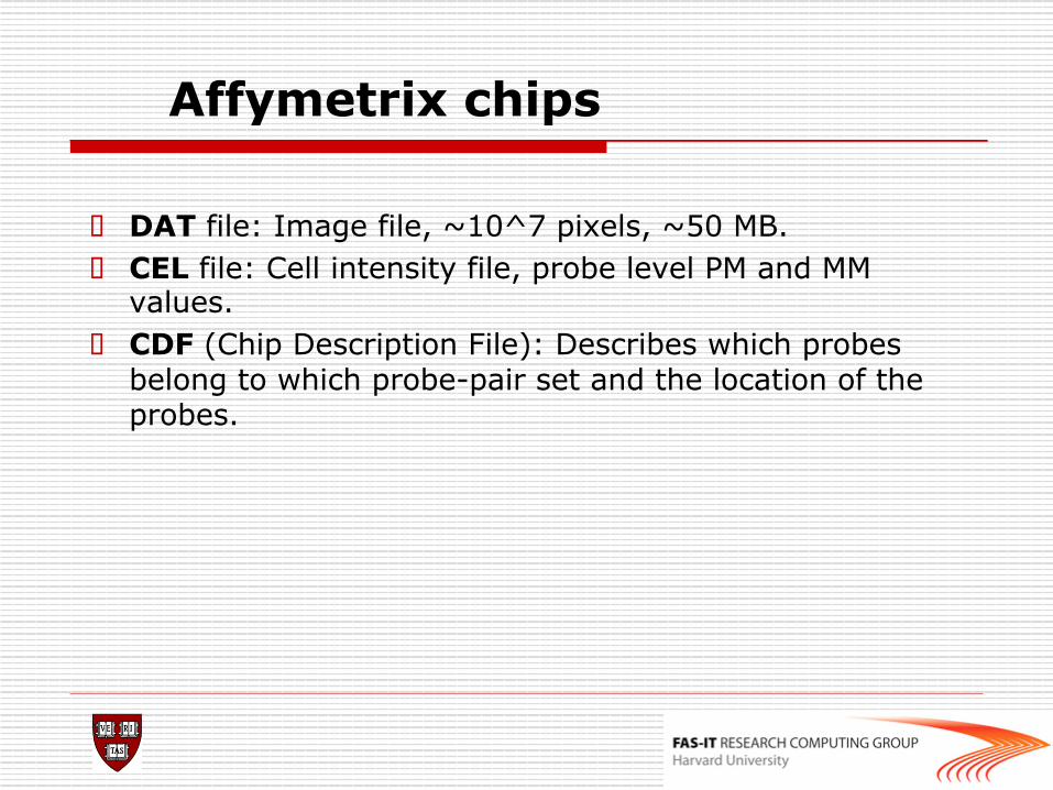
Affymetrix chips
o DAT file: Image file, ~10^7 pixels, ~50 MB. o CEL file: Cell intensity file, probe level PM and MM
values. o CDF (Chip Description File): Describes which probes
belong to which probe-pair set and the location of the probes.
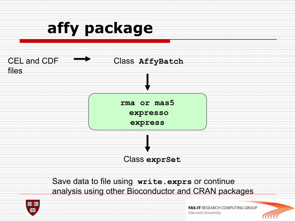
affy package
rma or mas5 expresso express
Class AffyBatch
Class exprSet
Save data to file using write.exprs or continue analysis using other Bioconductor and CRAN packages
CEL and CDF files
affy and simpleaffy package
o Class definitions for probe-level data: AffyBatch, ProbSet, Cdf, Cel. o Basic methods for manipulating microarray objects: printing, plotting,
subsetting. o Functions and widgets for data input from CEL and CDF files, and
automatic generation of microarray data objects. o Diagnostic plots: 2D spatial images, density plots, boxplots, MA-plots.
n image: 2D spatial color images of log intensities (AffyBatch, Cel). n boxplot: boxplots of log intensities (AffyBatch). n mva.pairs: scatter-plots with fitted curves (apply exprs, pm, or mm to AffyBatch object). n hist: density plots of log intensities (AffyBatch).
o Check RNA degradation and couple control metrics defined by affymetrix company library(simpleaffy) Data.qc<-qc(data) avbg(Data.qc) sfs(Data.qc) percent.present(Data.qc) ratios(Data.qc[,1:2])
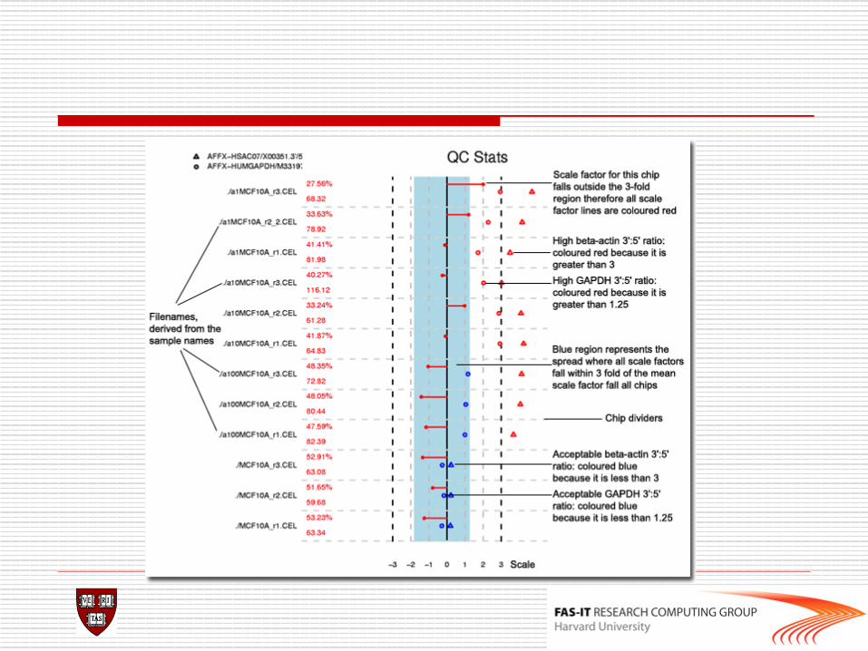
Quality control(2)
QC metrics o 1. Average background o 2. Scale factor o 3. Number of genes called present o 4. 3’ to 5’ ratios of actin and GAPDH o 5. Uses ordered probes in all probeset
to detect possible RNA degradation.
Lab
>library(affy) >library("simpleaffy") >data<-ReadAffy() >qc(data)->data.qc >avbg(data.qc) #comparable bg expected >sfs(data.qc) #within 3folds of each other expected >percent.present(data.qc) #extremely low value is a
#problem >ratios(data.qc) >AffyRNAdeg(data)->RNAdeg >plotAffyRNAdeg(RNAdeg) >summaryAffyRNAdeg(RNAdeg)
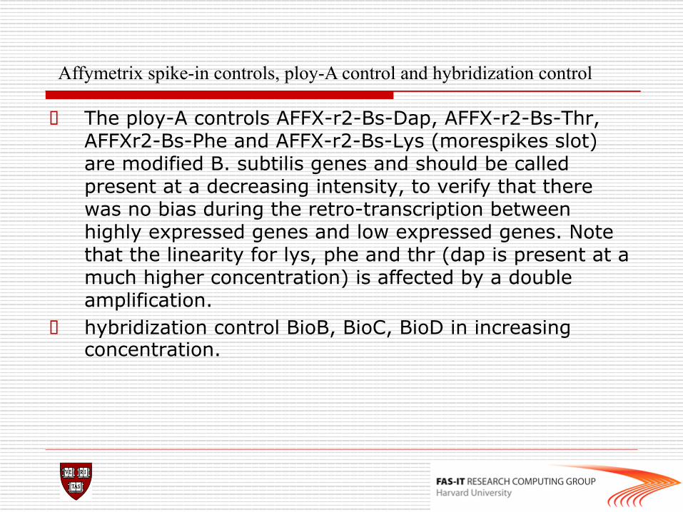
o The ploy-A controls AFFX-r2-Bs-Dap, AFFX-r2-Bs-Thr, AFFXr2-Bs-Phe and AFFX-r2-Bs-Lys (morespikes slot) are modified B. subtilis genes and should be called present at a decreasing intensity, to verify that there was no bias during the retro-transcription between highly expressed genes and low expressed genes. Note that the linearity for lys, phe and thr (dap is present at a much higher concentration) is affected by a double amplification.
o hybridization control BioB, BioC, BioD in increasing concentration.
Affymetrix spike-in controls, ploy-A control and hybridization control
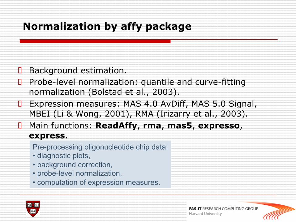
Normalization by affy package
o Background estimation. o Probe-level normalization: quantile and curve-fitting
normalization (Bolstad et al., 2003). o Expression measures: MAS 4.0 AvDiff, MAS 5.0 Signal,
MBEI (Li & Wong, 2001), RMA (Irizarry et al., 2003). o Main functions: ReadAffy, rma, mas5, expresso,
express. Pre-processing oligonucleotide chip data: • diagnostic plots, • background correction, • probe-level normalization, • computation of expression measures.
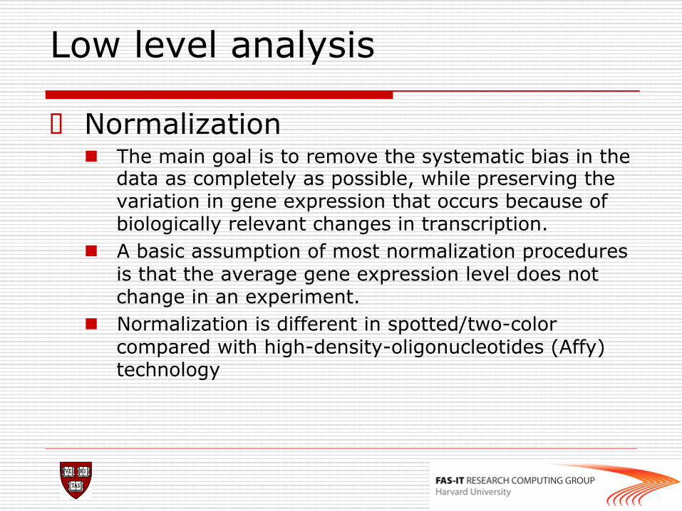
Low level analysis
o Normalization n The main goal is to remove the systematic bias in the
data as completely as possible, while preserving the variation in gene expression that occurs because of biologically relevant changes in transcription.
n A basic assumption of most normalization procedures is that the average gene expression level does not change in an experiment.
n Normalization is different in spotted/two-color compared with high-density-oligonucleotides (Affy) technology
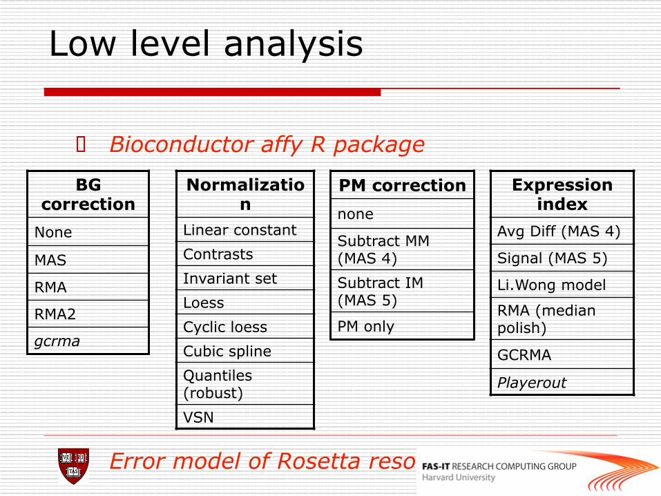
Low level analysis
o Bioconductor affy R package
o Error model of Rosetta resolver
Normalization
Linear constant Contrasts Invariant set Loess Cyclic loess Cubic spline Quantiles (robust) VSN
PM correction none
Subtract MM (MAS 4) Subtract IM (MAS 5)
PM only
BG correction
None
MAS
RMA
RMA2
gcrma
Expression index
Avg Diff (MAS 4)
Signal (MAS 5)
Li.Wong model
RMA (median polish)
GCRMA
Playerout
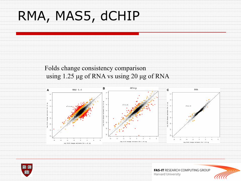
RMA, MAS5, dCHIP
Folds change consistency comparison using 1.25 µg of RNA vs using 20 µg of RNA
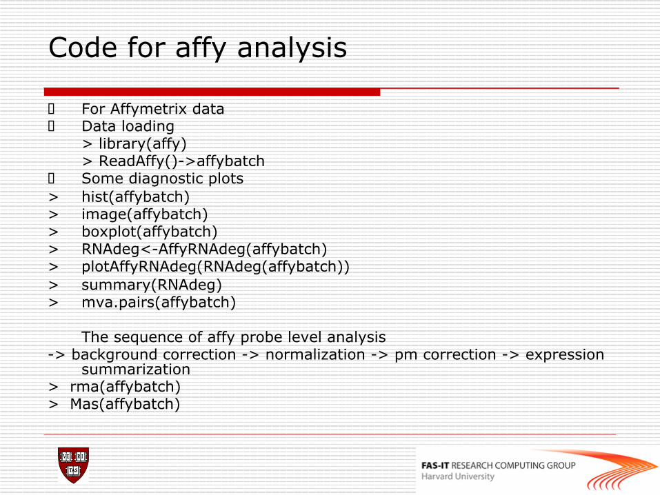
Code for affy analysis
o For Affymetrix data o Data loading
> library(affy) > ReadAffy()->affybatch
o Some diagnostic plots > hist(affybatch) > image(affybatch) > boxplot(affybatch) > RNAdeg<-AffyRNAdeg(affybatch) > plotAffyRNAdeg(RNAdeg(affybatch)) > summary(RNAdeg) > mva.pairs(affybatch)
The sequence of affy probe level analysis -> background correction -> normalization -> pm correction -> expression
summarization > rma(affybatch) > Mas(affybatch)
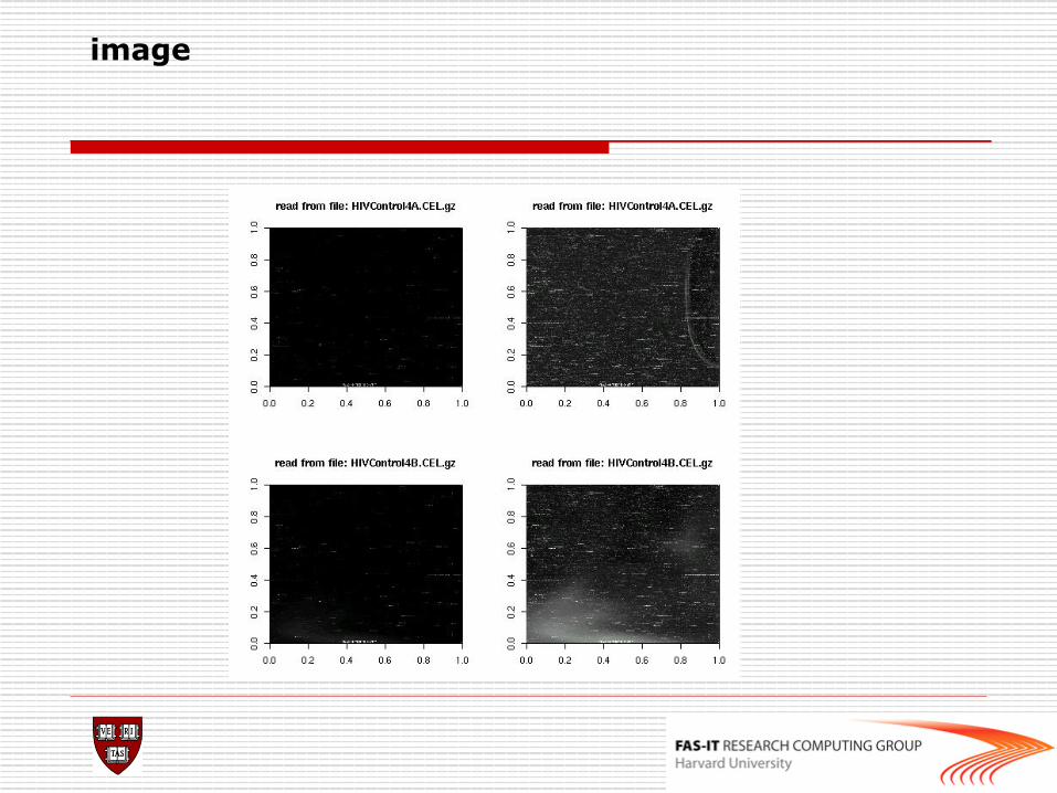
image
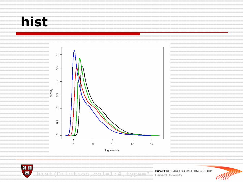
hist
hist(Dilution,col=1:4,type="l",lty=1,lwd=3)
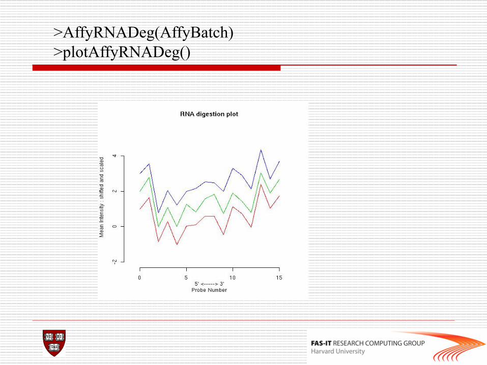
>AffyRNADeg(AffyBatch) >plotAffyRNADeg()
Differential Gene Expression
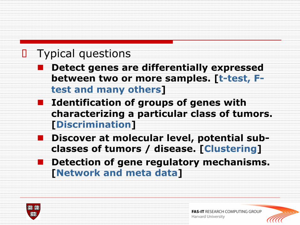
o Typical questions n Detect genes are differentially expressed
between two or more samples. [t-test, F-test and many others]
n Identification of groups of genes with characterizing a particular class of tumors. [Discrimination]
n Discover at molecular level, potential sub-classes of tumors / disease. [Clustering]
n Detection of gene regulatory mechanisms. [Network and meta data]
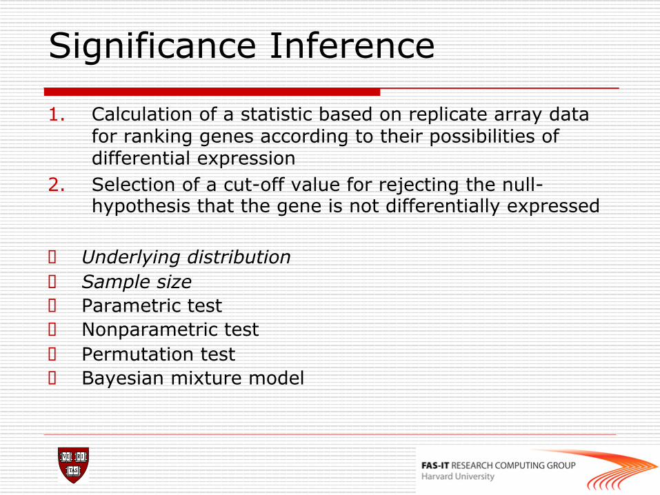
1. Calculation of a statistic based on replicate array data for ranking genes according to their possibilities of differential expression
2. Selection of a cut-off value for rejecting the null-hypothesis that the gene is not differentially expressed
o Underlying distribution o Sample size o Parametric test o Nonparametric test o Permutation test o Bayesian mixture model
Significance Inference
o Student’s T-test ti = (Mi/SEi) where SEi (standard error of Mi) = si/√n
o Introduces some conservative protection against outlier M-values and poor quality spots
o Limitations n large t-statistic can be driven by an
unrealistically small value for s n Suffers from multiple hypothesis testing problem n Suffers from inflated type I error
o Moderated t-statistic from limma package n Uses empirical Bayes to estimate a posterior variance
of the gene with the information borrow from all genes
n Smyth, G. K. (2004). Linear models and empirical Bayes methods for assessing differential expression in microarray experiments. Statistical Applications in Genetics and Molecular Biology 3, No. 1, Article 3.
Significance Inference
Ebayes: borrow information from ensemble of genes, a good strategy for small sample project, superior to t-test.
has more functions than just linear
modeling, it basically provides another ways for prepossessing, normalizing and plotting data as marray packages
Limma package
Significance Inference
o Fold change as a threshold cut-off is inadequate, even if it is an average of replicates
o Limitations: n Fixed threshold does not account for statistical
significance n Does not take into account of the variability of
the expression levels for each gene n Genes with larger variances have a good chance
of giving a large fold change even if they are not differentially expressed
n Inflated type I & type II errors
Statistical filtering
o Ultimately, what matters is biological relevance.
o P-values should help you evaluate the strength of the evidence, rather than being used as an absolute yardstick of significance.
o Statistical significance is not necessarily the same as biological significance.
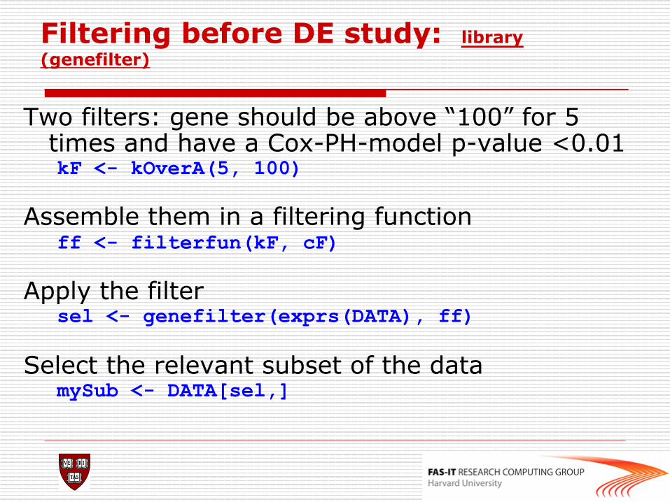
Filtering before DE study: library(genefilter)
Two filters: gene should be above “100” for 5 times and have a Cox-PH-model p-value <0.01 kF <- kOverA(5, 100)
Assemble them in a filtering function
ff <- filterfun(kF, cF) Apply the filter
sel <- genefilter(exprs(DATA), ff) Select the relevant subset of the data
mySub <- DATA[sel,]
Annotation and metadata
Biological metadata
o Biological attributes that can be applied to the experimental data. o E.g. for genes
n chromosomal location; n gene annotation (LocusLink, GO); n relevant literature (PubMed).
o Biological metadata sets are large, evolving rapidly, and typically distributed via the WWW.
o Tools: annotate, annaffy, and AnnBuilder packages, and annotation data packages.
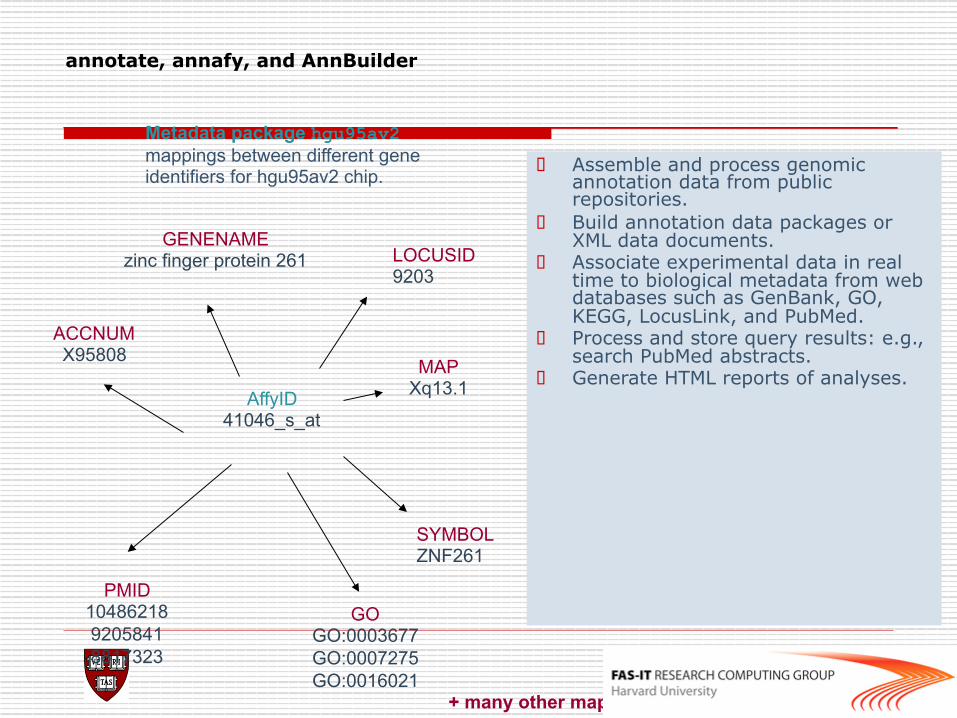
annotate, annafy, and AnnBuilder
o Assemble and process genomic annotation data from public repositories.
o Build annotation data packages or XML data documents.
o Associate experimental data in real time to biological metadata from web databases such as GenBank, GO, KEGG, LocusLink, and PubMed.
o Process and store query results: e.g., search PubMed abstracts.
o Generate HTML reports of analyses. AffyID
41046_s_at
ACCNUM X95808
LOCUSID 9203
SYMBOL ZNF261
GENENAME zinc finger protein 261
MAP Xq13.1
PMID 10486218 9205841 8817323
GO GO:0003677 GO:0007275 GO:0016021
+ many other mappings
Metadata package hgu95av2 mappings between different gene identifiers for hgu95av2 chip.
Distances, Prediction, and Cluster Analysis
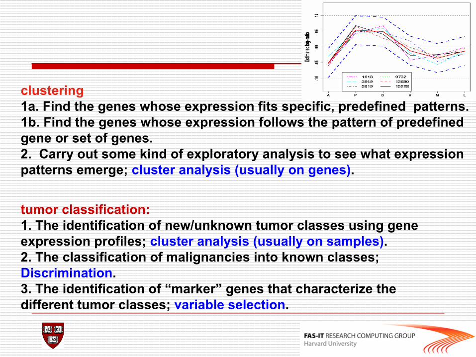
tumor classification: 1. The identification of new/unknown tumor classes using gene expression profiles; cluster analysis (usually on samples). 2. The classification of malignancies into known classes; Discrimination. 3. The identification of “marker” genes that characterize the different tumor classes; variable selection.
clustering 1a. Find the genes whose expression fits specific, predefined patterns. 1b. Find the genes whose expression follows the pattern of predefined gene or set of genes. 2. Carry out some kind of exploratory analysis to see what expression patterns emerge; cluster analysis (usually on genes).
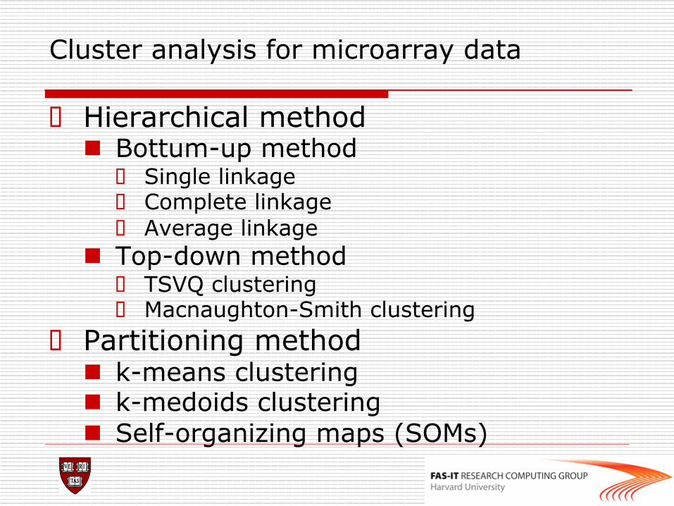
Cluster analysis for microarray data
o Hierarchical method n Bottum-up method
o Single linkage o Complete linkage o Average linkage
n Top-down method o TSVQ clustering o Macnaughton-Smith clustering
o Partitioning method n k-means clustering n k-medoids clustering n Self-organizing maps (SOMs)
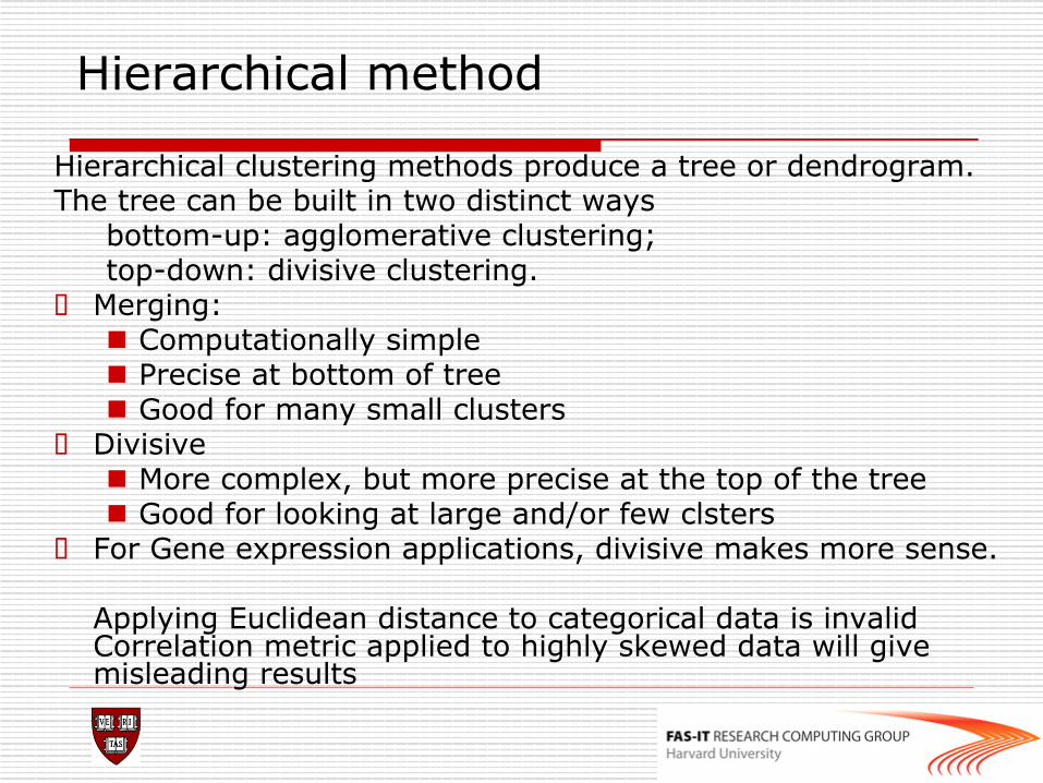
Hierarchical method
Hierarchical clustering methods produce a tree or dendrogram. The tree can be built in two distinct ways
bottom-up: agglomerative clustering; top-down: divisive clustering.
o Merging: n Computationally simple n Precise at bottom of tree n Good for many small clusters
o Divisive n More complex, but more precise at the top of the tree n Good for looking at large and/or few clsters
o For Gene expression applications, divisive makes more sense. Applying Euclidean distance to categorical data is invalid Correlation metric applied to highly skewed data will give misleading results
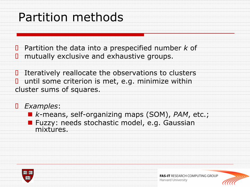
Partition methods
o Partition the data into a prespecified number k of o mutually exclusive and exhaustive groups.
o Iteratively reallocate the observations to clusters o until some criterion is met, e.g. minimize within cluster sums of squares.
o Examples: n k-means, self-organizing maps (SOM), PAM, etc.; n Fuzzy: needs stochastic model, e.g. Gaussian
mixtures.
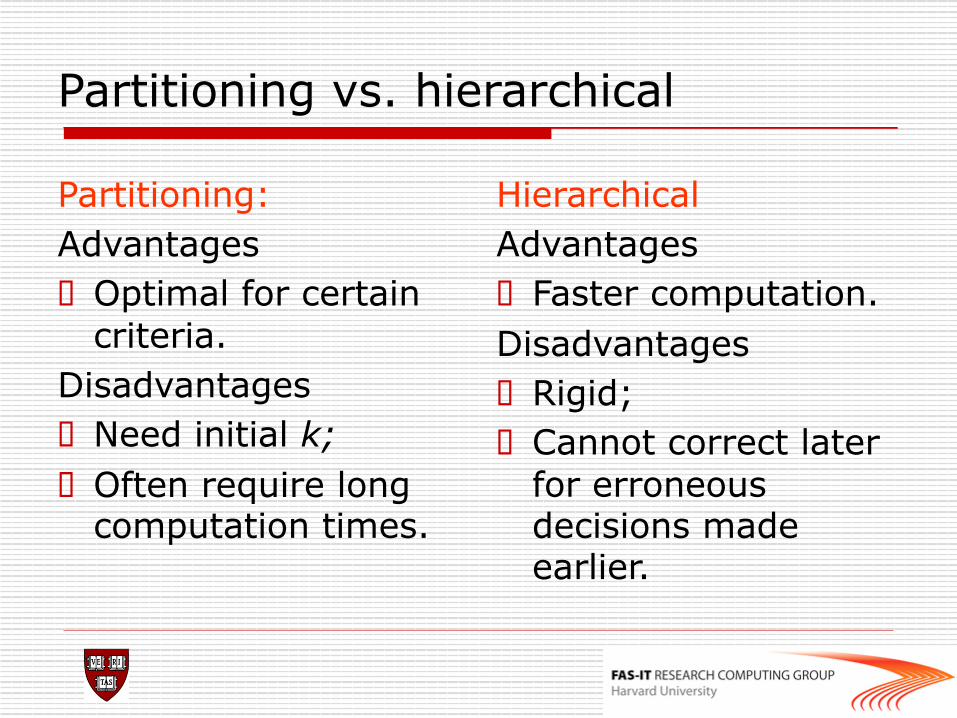
Partitioning vs. hierarchical
Partitioning: Advantages o Optimal for certain
criteria. Disadvantages o Need initial k; o Often require long
computation times.
Hierarchical Advantages o Faster computation. Disadvantages o Rigid; o Cannot correct later
for erroneous decisions made earlier.
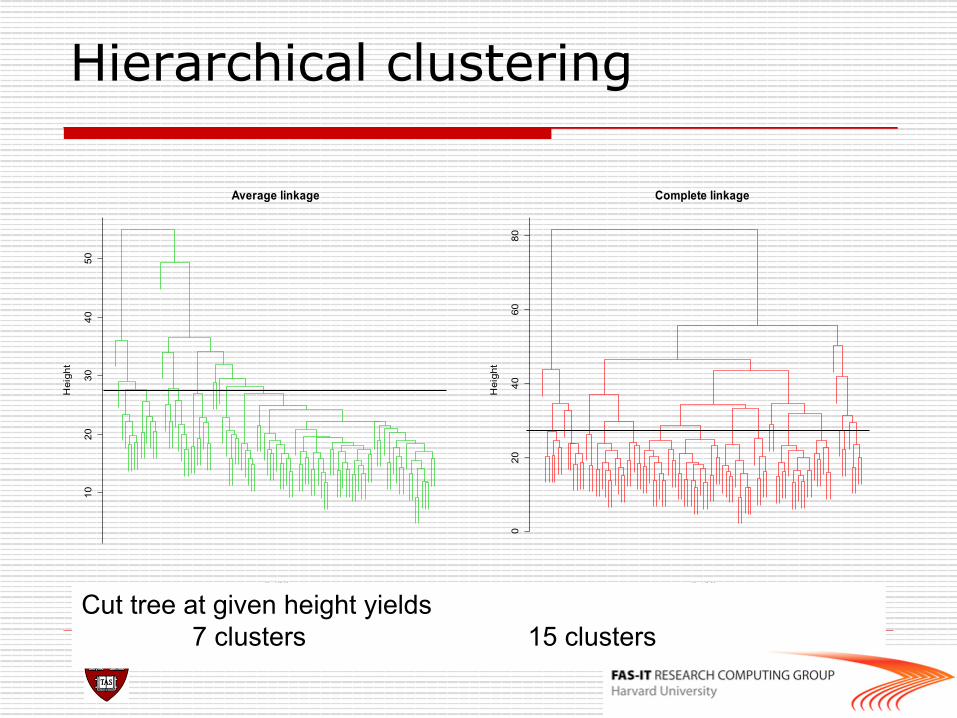
Hierarchical clustering 10
2030
4050
Average linkage
hclust (*, "average")dist(X)
Hei
ght
020
4060
80
Complete linkage
hclust (*, "complete")dist(X)
Hei
ght
Cut tree at given height yields 7 clusters 15 clusters
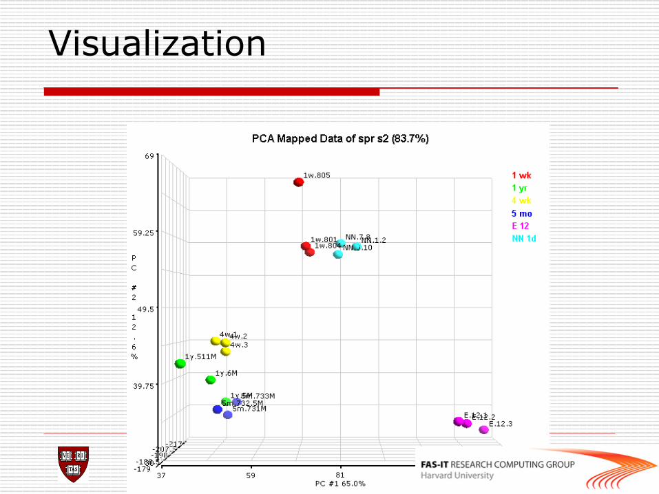
Visualization
o Principal components analysis (PCA), an exploratory technique that reduces data dimensionality to 2 or 3 dimensional space.
o For a matrix of m genes x n samples, create a new covariance matrix of size n x n
o Thus transform some large number of variables into a smaller number of uncorrelated variables called principal components (PCs).
Visualization
Distances
o Microarray data analysis often involves n clustering genes and/or samples; n classifying genes and/or samples.
o Both types of analyses are based on a measure of distance (or similarity) between genes or samples.
o R has a number of functions for computing and plotting distance and similarity matrices.
Distances
o Distance functions n dist (mva): Euclidean, Manhattan, Canberra, binary; n daisy (cluster).
o Correlation functions n cor, cov.wt.
o Plotting functions n image; n plotcorr (ellipse); n plot.cor, plot.mat (sma).
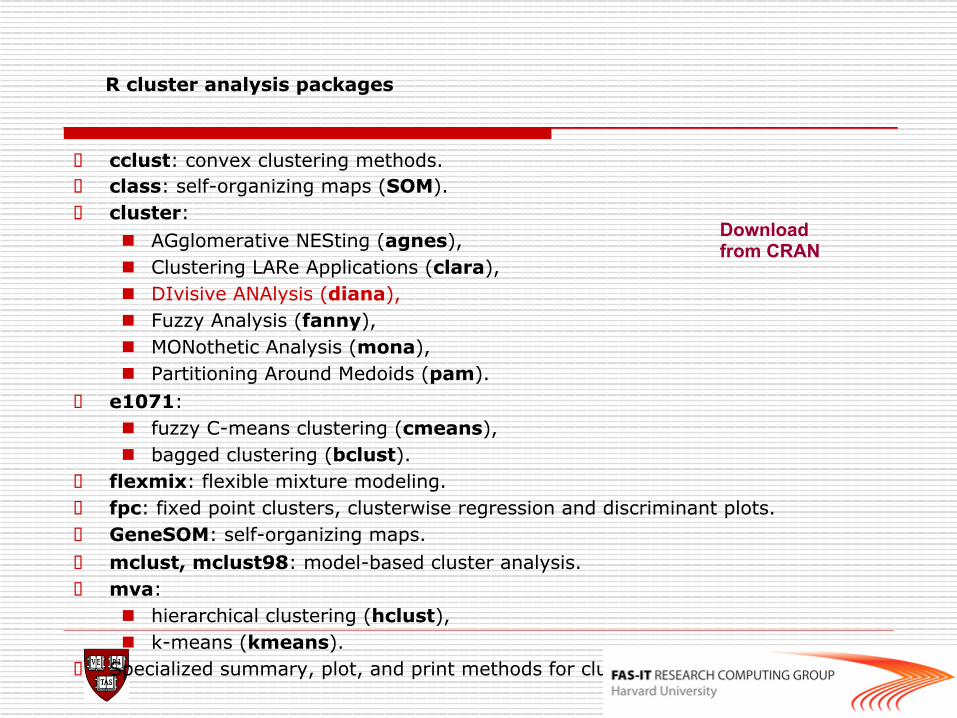
R cluster analysis packages
o cclust: convex clustering methods. o class: self-organizing maps (SOM). o cluster:
n AGglomerative NESting (agnes), n Clustering LARe Applications (clara), n DIvisive ANAlysis (diana), n Fuzzy Analysis (fanny), n MONothetic Analysis (mona), n Partitioning Around Medoids (pam).
o e1071: n fuzzy C-means clustering (cmeans), n bagged clustering (bclust).
o flexmix: flexible mixture modeling. o fpc: fixed point clusters, clusterwise regression and discriminant plots. o GeneSOM: self-organizing maps. o mclust, mclust98: model-based cluster analysis. o mva:
n hierarchical clustering (hclust), n k-means (kmeans).
o Specialized summary, plot, and print methods for clustering results.
Download from CRAN
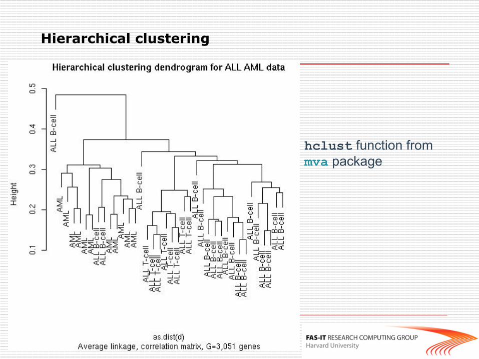
hclust function from mva package
Hierarchical clustering
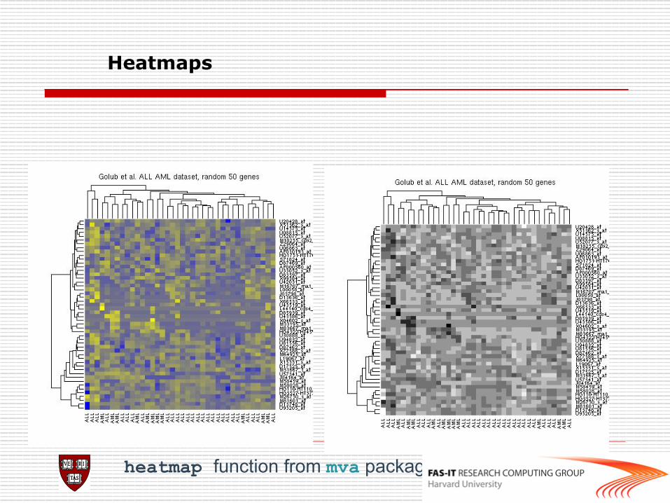
Heatmaps
heatmap function from mva package
Class prediction
o Old and extensive literature on class prediction, in statistics and machine learning.
o Examples of classifiers n nearest neighbor classifiers (k-NN); n discriminant analysis: linear, quadratic, logistic; n neural networks; n classification trees; n support vector machines.
o Aggregated classifiers: bagging and boosting
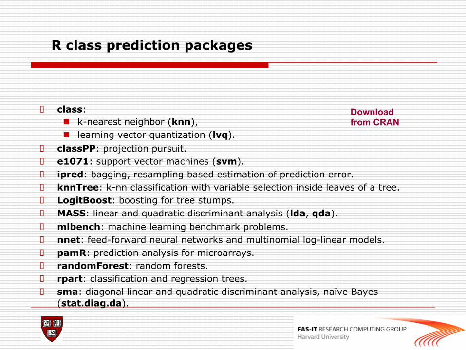
R class prediction packages
o class: n k-nearest neighbor (knn), n learning vector quantization (lvq).
o classPP: projection pursuit. o e1071: support vector machines (svm). o ipred: bagging, resampling based estimation of prediction error. o knnTree: k-nn classification with variable selection inside leaves of a tree. o LogitBoost: boosting for tree stumps. o MASS: linear and quadratic discriminant analysis (lda, qda). o mlbench: machine learning benchmark problems. o nnet: feed-forward neural networks and multinomial log-linear models. o pamR: prediction analysis for microarrays. o randomForest: random forests. o rpart: classification and regression trees. o sma: diagonal linear and quadratic discriminant analysis, naïve Bayes
(stat.diag.da).
Download from CRAN
Lab
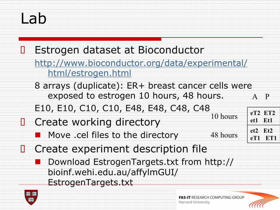
o Estrogen dataset at Bioconductor http://www.bioconductor.org/data/experimental/
html/estrogen.html 8 arrays (duplicate): ER+ breast cancer cells were
exposed to estrogen 10 hours, 48 hours. E10, E10, C10, C10, E48, E48, C48, C48
o Create working directory n Move .cel files to the directory
o Create experiment description file n Download EstrogenTargets.txt from http://
bioinf.wehi.edu.au/affylmGUI/EstrogenTargets.txt
eT2 ET2 et1 Et1 et2 Et2 eT1 ET1
10 hours
48 hours
A P
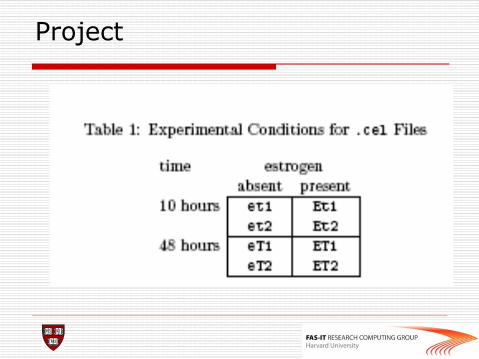
Project
Brief introduction: data gives results from a 2x2 factorial experiment on MCF7 breast cancer cells using Affymetrix HGU95av2 arrays. The factors in this experiment were estrogen (present or absent) and length of exposure (10 or 48 hours). The aim of the study is the identify genes which respond to estrogen and to classify these into early and late responders. Genes which respond early are putative direct-target genes while those which respond late are probably downstream targets in the molecular pathway This experiment studied the effect of estrogen on the gene expression in estrogen receptor positive breast cancer cells over time. After serum starvation, samples were exposed to estrogen, and mRNA was harvested at two time points (10 or 48 hours). The control samples were not exposed to estrogen and were harvested at the same time points. Table 1 shows the experimental design, and corresponding samples names. The full data set (12,625 probes, 32 samples) and its analysis are discussed in Scholtens, et al. Analyzing Factorial Designed Microarray Experiments.
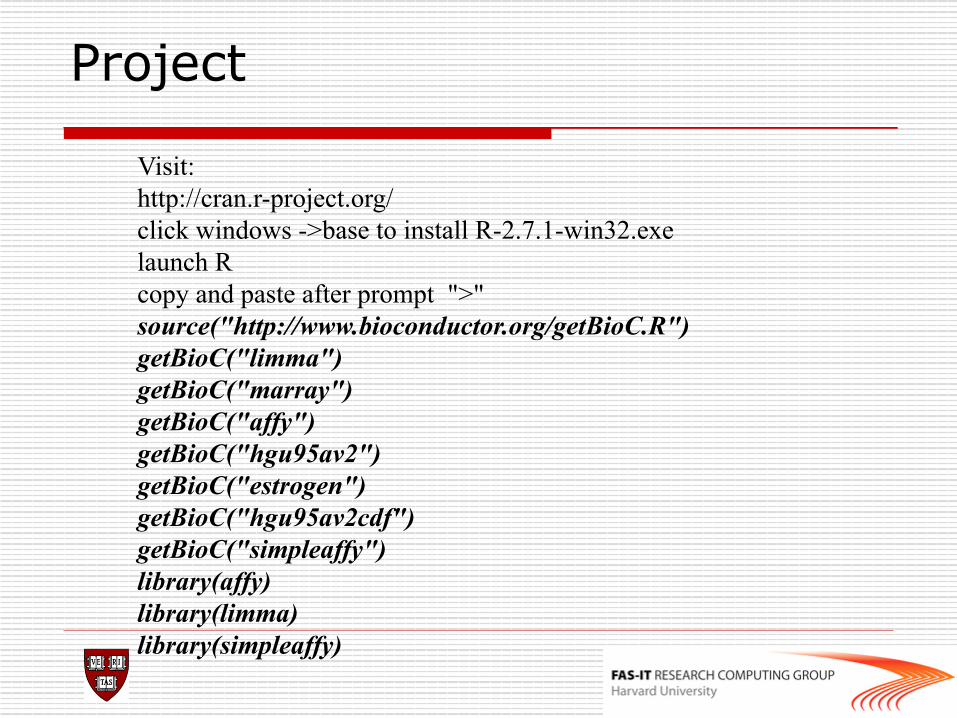
Project
Visit: http://cran.r-project.org/ click windows ->base to install R-2.7.1-win32.exe launch R copy and paste after prompt ">" source("http://www.bioconductor.org/getBioC.R") getBioC("limma") getBioC("marray") getBioC("affy") getBioC("hgu95av2") getBioC("estrogen") getBioC("hgu95av2cdf") getBioC("simpleaffy") library(affy) library(limma) library(simpleaffy)
Project
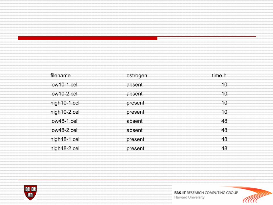
filename estrogen time.h
low10-1.cel absent 10
low10-2.cel absent 10
high10-1.cel present 10
high10-2.cel present 10
low48-1.cel absent 48
low48-2.cel absent 48
high48-1.cel present 48
high48-2.cel present 48
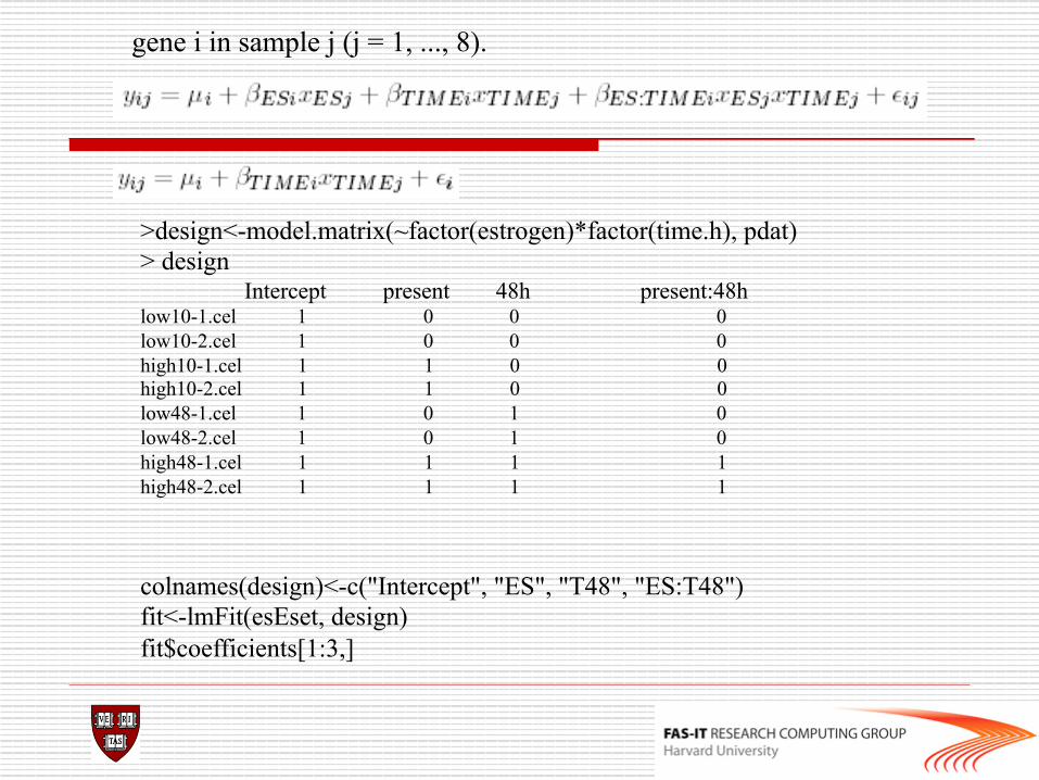
colnames(design)<-c("Intercept", "ES", "T48", "ES:T48") fit<-lmFit(esEset, design) fit$coefficients[1:3,]
gene i in sample j (j = 1, ..., 8).
>design<-model.matrix(~factor(estrogen)*factor(time.h), pdat) > design Intercept present 48h present:48h low10-1.cel 1 0 0 0 low10-2.cel 1 0 0 0 high10-1.cel 1 1 0 0 high10-2.cel 1 1 0 0 low48-1.cel 1 0 1 0 low48-2.cel 1 0 1 0 high48-1.cel 1 1 1 1 high48-2.cel 1 1 1 1
Project
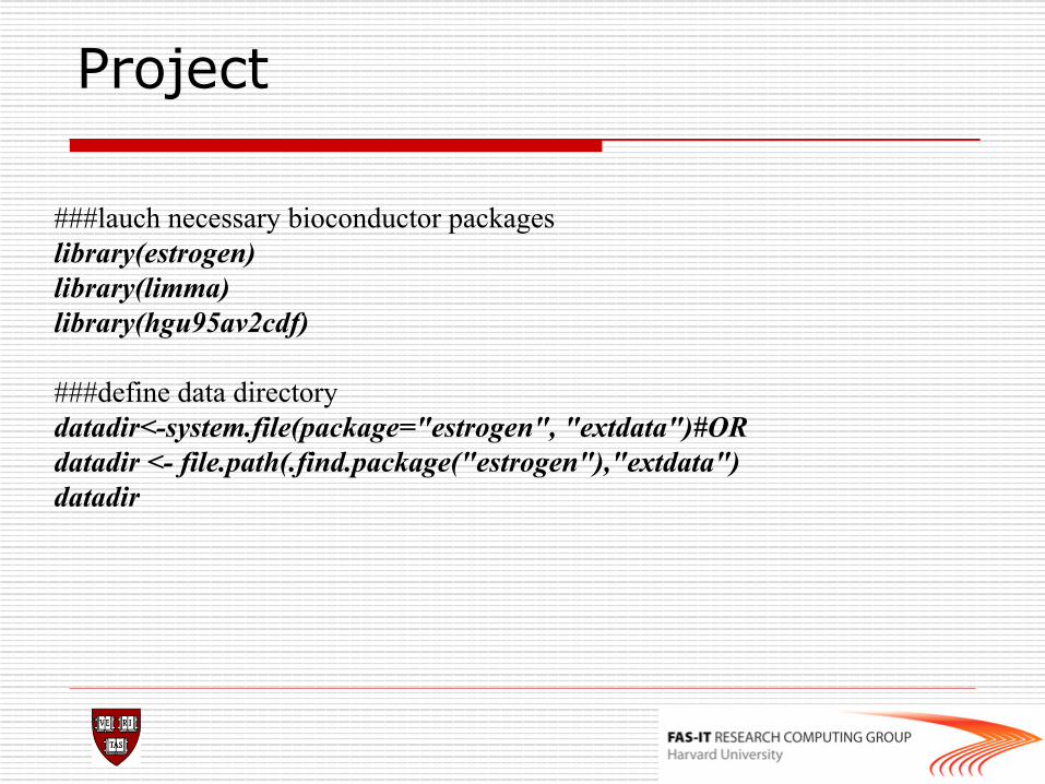
###lauch necessary bioconductor packages library(estrogen) library(limma) library(hgu95av2cdf) ###define data directory datadir<-system.file(package="estrogen", "extdata")#OR datadir <- file.path(.find.package("estrogen"),"extdata") datadir
Project
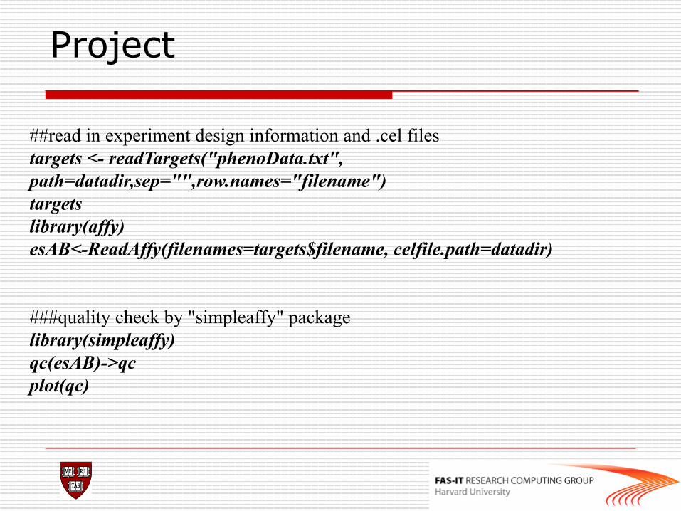
##read in experiment design information and .cel files targets <- readTargets("phenoData.txt", path=datadir,sep="",row.names="filename") targets library(affy) esAB<-ReadAffy(filenames=targets$filename, celfile.path=datadir) ###quality check by "simpleaffy" package library(simpleaffy) qc(esAB)->qc plot(qc)
Project
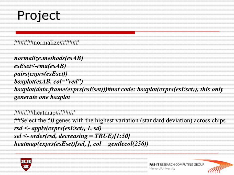
######normalize###### normalize.methods(esAB) esEset<-rma(esAB) pairs(exprs(esEset)) boxplot(esAB, col="red") boxplot(data.frame(exprs(esEset)))#not code: boxplot(exprs(esEset)), this only generate one boxplot ######heatmap###### ##Select the 50 genes with the highest variation (standard deviation) across chips rsd <- apply(exprs(esEset), 1, sd) sel <- order(rsd, decreasing = TRUE)[1:50] heatmap(exprs(esEset)[sel, ], col = gentlecol(256))
Project
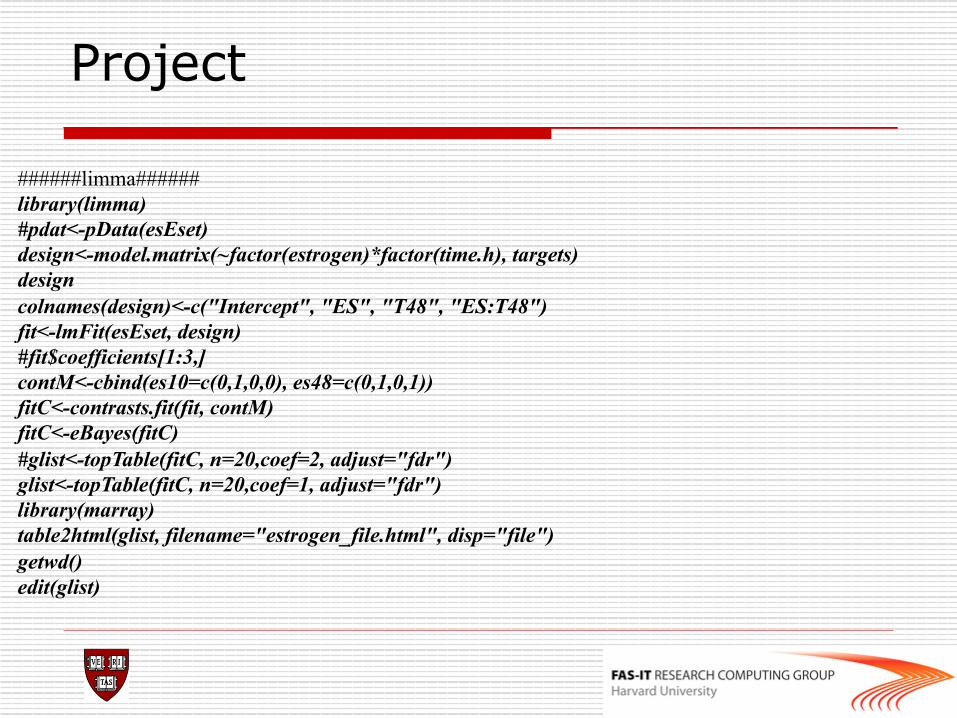
######limma###### library(limma) #pdat<-pData(esEset) design<-model.matrix(~factor(estrogen)*factor(time.h), targets) design colnames(design)<-c("Intercept", "ES", "T48", "ES:T48") fit<-lmFit(esEset, design) #fit$coefficients[1:3,] contM<-cbind(es10=c(0,1,0,0), es48=c(0,1,0,1)) fitC<-contrasts.fit(fit, contM) fitC<-eBayes(fitC) #glist<-topTable(fitC, n=20,coef=2, adjust="fdr") glist<-topTable(fitC, n=20,coef=1, adjust="fdr") library(marray) table2html(glist, filename="estrogen_file.html", disp="file") getwd() edit(glist)
Project
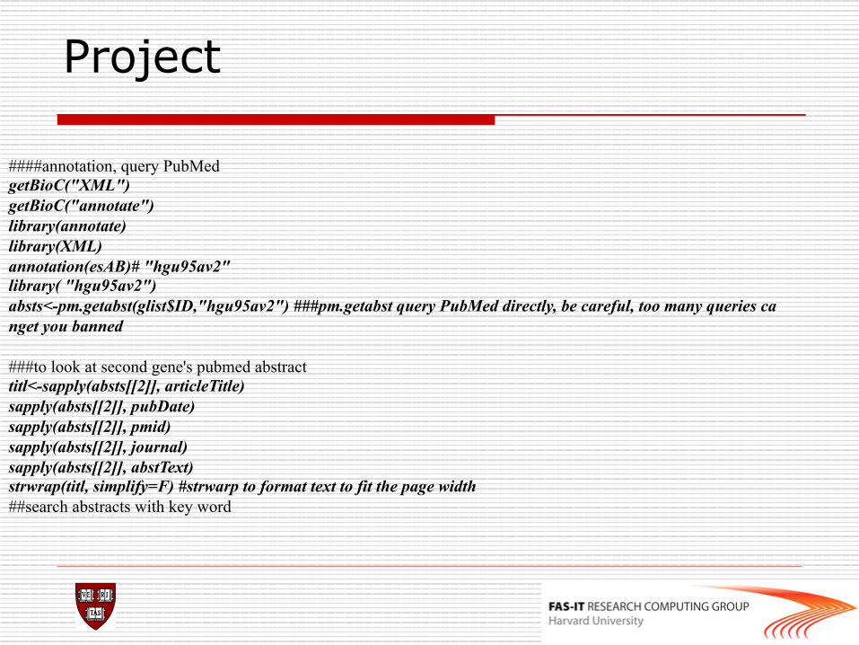
####annotation, query PubMed getBioC("XML") getBioC("annotate") library(annotate) library(XML) annotation(esAB)# "hgu95av2" library( "hgu95av2") absts<-pm.getabst(glist$ID,"hgu95av2") ###pm.getabst query PubMed directly, be careful, too many queries ca nget you banned ###to look at second gene's pubmed abstract titl<-sapply(absts[[2]], articleTitle) sapply(absts[[2]], pubDate) sapply(absts[[2]], pmid) sapply(absts[[2]], journal) sapply(absts[[2]], abstText) strwrap(titl, simplify=F) #strwarp to format text to fit the page width ##search abstracts with key word
Project
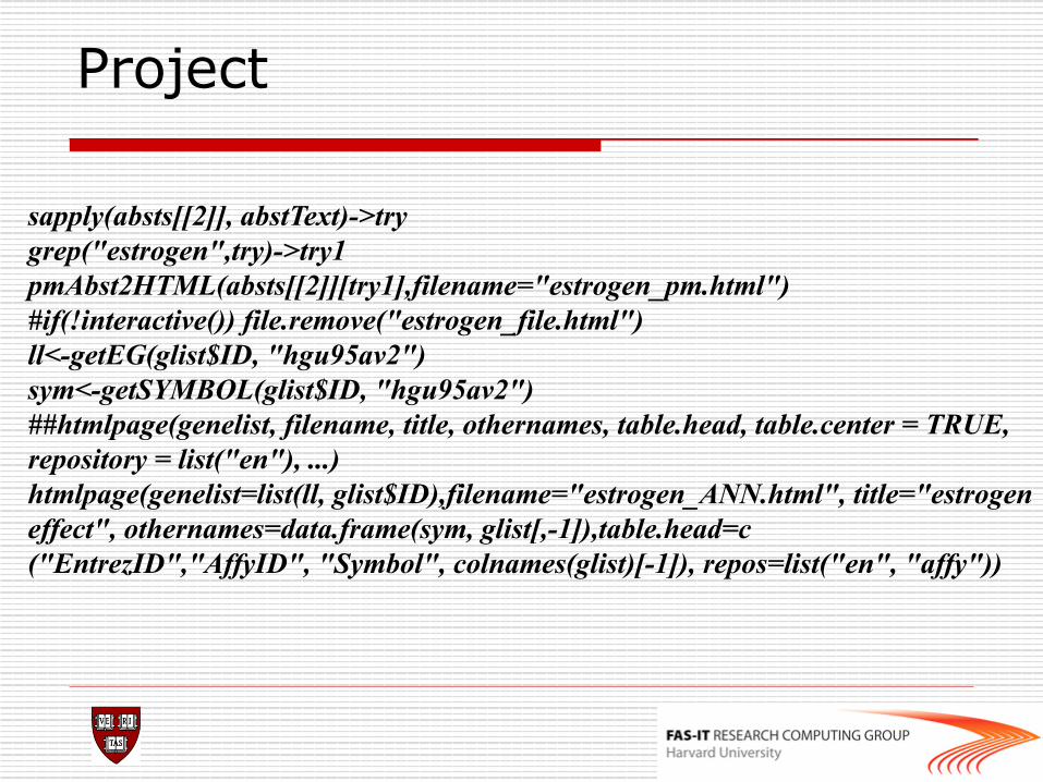
sapply(absts[[2]], abstText)->try grep("estrogen",try)->try1 pmAbst2HTML(absts[[2]][try1],filename="estrogen_pm.html") #if(!interactive()) file.remove("estrogen_file.html") ll<-getEG(glist$ID, "hgu95av2") sym<-getSYMBOL(glist$ID, "hgu95av2") ##htmlpage(genelist, filename, title, othernames, table.head, table.center = TRUE, repository = list("en"), ...) htmlpage(genelist=list(ll, glist$ID),filename="estrogen_ANN.html", title="estrogen effect", othernames=data.frame(sym, glist[,-1]),table.head=c("EntrezID","AffyID", "Symbol", colnames(glist)[-1]), repos=list("en", "affy"))
Project
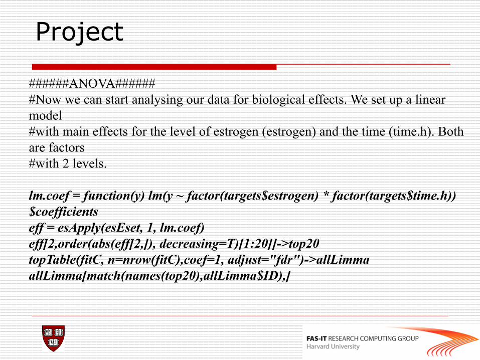
######ANOVA###### #Now we can start analysing our data for biological effects. We set up a linear model #with main effects for the level of estrogen (estrogen) and the time (time.h). Both are factors #with 2 levels. lm.coef = function(y) lm(y ~ factor(targets$estrogen) * factor(targets$time.h))$coefficients eff = esApply(esEset, 1, lm.coef) eff[2,order(abs(eff[2,]), decreasing=T)[1:20]]->top20 topTable(fitC, n=nrow(fitC),coef=1, adjust="fdr")->allLimma allLimma[match(names(top20),allLimma$ID),]
Project
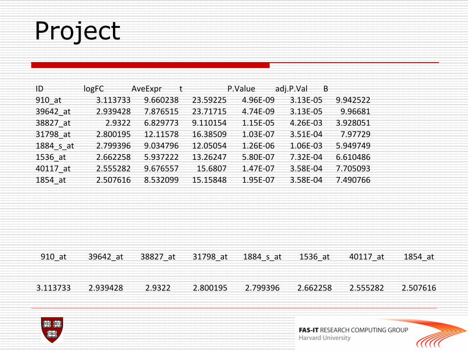
ID logFC AveExpr t P.Value adj.P.Val B 910_at 3.113733 9.660238 23.59225 4.96E-‐09 3.13E-‐05 9.942522 39642_at 2.939428 7.876515 23.71715 4.74E-‐09 3.13E-‐05 9.96681 38827_at 2.9322 6.829773 9.110154 1.15E-‐05 4.26E-‐03 3.928051 31798_at 2.800195 12.11578 16.38509 1.03E-‐07 3.51E-‐04 7.97729 1884_s_at 2.799396 9.034796 12.05054 1.26E-‐06 1.06E-‐03 5.949749 1536_at 2.662258 5.937222 13.26247 5.80E-‐07 7.32E-‐04 6.610486 40117_at 2.555282 9.676557 15.6807 1.47E-‐07 3.58E-‐04 7.705093 1854_at 2.507616 8.532099 15.15848 1.95E-‐07 3.58E-‐04 7.490766
910_at 39642_at 38827_at 31798_at 1884_s_at 1536_at 40117_at 1854_at
3.113733 2.939428 2.9322 2.800195 2.799396 2.662258 2.555282 2.507616
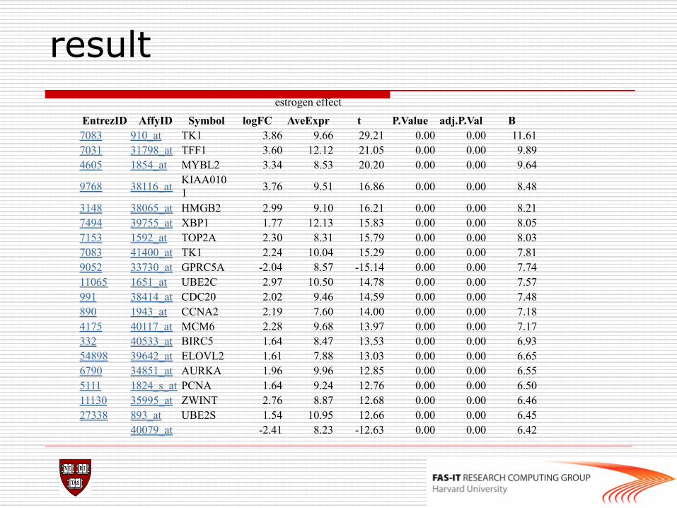
result estrogen effect
EntrezID AffyID Symbol logFC AveExpr t P.Value adj.P.Val B 7083 910_at TK1 3.86 9.66 29.21 0.00 0.00 11.61 7031 31798_at TFF1 3.60 12.12 21.05 0.00 0.00 9.89 4605 1854_at MYBL2 3.34 8.53 20.20 0.00 0.00 9.64
9768 38116_at KIAA0101 3.76 9.51 16.86 0.00 0.00 8.48
3148 38065_at HMGB2 2.99 9.10 16.21 0.00 0.00 8.21 7494 39755_at XBP1 1.77 12.13 15.83 0.00 0.00 8.05 7153 1592_at TOP2A 2.30 8.31 15.79 0.00 0.00 8.03 7083 41400_at TK1 2.24 10.04 15.29 0.00 0.00 7.81 9052 33730_at GPRC5A -2.04 8.57 -15.14 0.00 0.00 7.74 11065 1651_at UBE2C 2.97 10.50 14.78 0.00 0.00 7.57 991 38414_at CDC20 2.02 9.46 14.59 0.00 0.00 7.48 890 1943_at CCNA2 2.19 7.60 14.00 0.00 0.00 7.18 4175 40117_at MCM6 2.28 9.68 13.97 0.00 0.00 7.17 332 40533_at BIRC5 1.64 8.47 13.53 0.00 0.00 6.93 54898 39642_at ELOVL2 1.61 7.88 13.03 0.00 0.00 6.65 6790 34851_at AURKA 1.96 9.96 12.85 0.00 0.00 6.55 5111 1824_s_at PCNA 1.64 9.24 12.76 0.00 0.00 6.50 11130 35995_at ZWINT 2.76 8.87 12.68 0.00 0.00 6.46 27338 893_at UBE2S 1.54 10.95 12.66 0.00 0.00 6.45 40079_at -2.41 8.23 -12.63 0.00 0.00 6.42
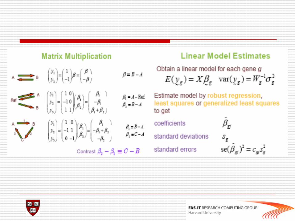
limma package
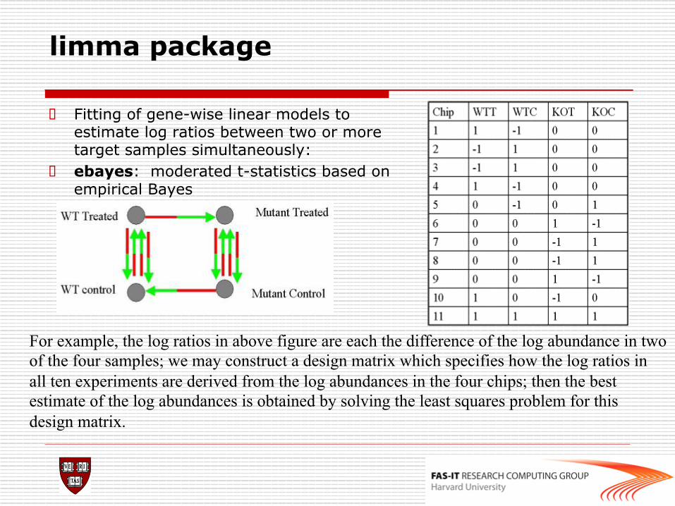
o Fitting of gene-wise linear models to estimate log ratios between two or more target samples simultaneously:
o ebayes: moderated t-statistics based on empirical Bayes
For example, the log ratios in above figure are each the difference of the log abundance in two of the four samples; we may construct a design matrix which specifies how the log ratios in all ten experiments are derived from the log abundances in the four chips; then the best estimate of the log abundances is obtained by solving the least squares problem for this design matrix.