Embed Size (px)
Citation preview
The University of Southern Mississippi The University of Southern Mississippi
The Aquila Digital Community The Aquila Digital Community
Dissertations
Spring 5-2011
Microarray Data Mining and Gene Regulatory Network Analysis Microarray Data Mining and Gene Regulatory Network Analysis
Ying Li University of Southern Mississippi
Follow this and additional works at: https://aquila.usm.edu/dissertations
Part of the Computational Biology Commons
Recommended Citation Recommended Citation Li, Ying, "Microarray Data Mining and Gene Regulatory Network Analysis" (2011). Dissertations. 477. https://aquila.usm.edu/dissertations/477
This Dissertation is brought to you for free and open access by The Aquila Digital Community. It has been accepted for inclusion in Dissertations by an authorized administrator of The Aquila Digital Community. For more information, please contact [email protected].

The University of Southern Mississippi
MICROARRAY DATA MINING AND GENE REGULATORY
NETWORK ANALYSIS
by
Ying Li
A DissertationSubmitted to the Graduate School
of The University of Southern Mississippiin Partial Fulfillment of the Requirements
for the Degree of Doctor of Philosophy
May 2011
ABSTRACT
MICROARRAY DATA MINING AND
GENE REGULATORY NETWORK ANALYSIS
by Ying Li
May 2011
The novel molecular biological technology, microarray, makes it feasible to obtain
quantitative measurements of expression of thousands of genes present in a biological
sample simultaneously. Genome-wide expression data generated from this technology are
promising to uncover the implicit, previously unknown biological knowledge. In this
study, several problems about microarray data mining techniques were investigated,
including feature(gene) selection, classifier genes identification, generation of reference
genetic interaction network for non-model organisms and gene regulatory network
reconstruction using time-series gene expression data. The limitations of most of the
existing computational models employed to infer gene regulatory network lie in that they
either suffer from low accuracy or computational complexity. To overcome such
limitations, the following strategies were proposed to integrate bioinformatics data
mining techniques with existing GRN inference algorithms, which enables the discovery
of novel biological knowledge. An integrated statistical and machine learning (ISML)
pipeline was developed for feature selection and classifier genes identification to solve
the challenges of the curse of dimensionality problem as well as the huge search space.
Using the selected classifier genes as seeds, a scale-up technique is applied to search
through major databases of genetic interaction networks, metabolic pathways, etc.
ii
By curating relevant genes and blasting genomic sequences of non-model organisms
against well-studied genetic model organisms, a reference gene regulatory network for
less-studied organisms was built and used both as prior knowledge and model validation
for GRN reconstructions. Networks of gene interactions were inferred using a Dynamic
Bayesian Network (DBN) approach and were analyzed for elucidating the dynamics
caused by perturbations. Our proposed pipelines were applied to investigate molecular
mechanisms for chemical-induced reversible neurotoxicity.
iii

COPYRIGHT BY
YING LI
2011

The University of Southern Mississippi
MICROARRAY DATA MINING AND GENE REGULATORY
NETWORK ANALYSIS
by
Ying Li
A DissertationSubmitted to the Graduate School
of The University of Southern Mississippiin Partial Fulfillment of the Requirements
for the Degree of Doctor of Philosophy
Approved:
Chaoyang ZhangDirector
____ Nan Wang______________________
____ Ping Gong______________________
Edward J Perkins
Andrew Strelzoff
Dean of the Graduate SchoolSusan A Siltanen
May 2011

ACKNOWLEDGMENTS
I would like to thank Dr. Nan Wang, Dr. Chaoyang Zhang, and all the other
committee members, Dr. Ping Gong, Dr. Edward J. Perkins, and Dr. Andrew Strelzoff,
for their suggestions and advice to improve my work during the whole process. I
gratefully acknowledge my advisors, Dr. Wang and Dr. Zhang, for their generous help in
the past four years. Along the path of research that has led to this dissertation, they have
constantly been there to provide me guidance, support and suggestions. I also would like
to thank Dr. Ping Gong and Dr. Edward Perkins for their comments and for providing
high-quality data during my doctoral research.
I am forever indebted to my parents, who have been extremely supportive and helpful
despite living thousands miles away. My father always encourages me to do what I want
to do, and my mother believes I am the best in the world, which gives me a lot of
confidence. I am especially thankful to all other collaborators in Engineer Research and
Development Center Environmental Lab in Vicksburg, MS. They gave me a lot of help
when I was working there during my Ph.D. program.
iv
TABLE OF CONTENTS
ABSTRACT ....................................................................................................................... ii
ACKNOWLEDGMENTS ................................................................................................ iv
LIST OF TABLES............................................................................................................ vii
LIST OF ILLUSTRATIONS............................................................................................. ix
CHAPTER
I. INTRODUCTION.......................................................................................1
Biological BackgroundDNA Microarray TechnologyMicroarray Data AnalysisContributionsDissertation Organization
II. REVIEW OF MICROARRAY DATA MINING ......................................13
Microarray Experiments and Data GenerationMicroarray Data PreprocessingIdentification of Differentially Expressed Genes (DEGs)Feature SelectionInference of Gene Regulatory Networks (GRNs)
III. IDENTIFY CLASSIFIER GENES USING ISML PIPELINE..................26
Integrated Statistical and Machine Learning (ISML) PipelineFeature Filtering by Statistical AnalysisClassifier Gene Selection and RankingOptimization by Machine Learning ApproachesIdentification of Significant Pathways
IV. REFNET: A TOOLBOX TO RETRIEVE REFERENCE NETWORK.....37
Basic Local Alignment Search Tool (BLAST)KEGG Metabolic Pathways and GRN DatabaseRefNet: Reference Network for Non-Model OrganismsInterpretation of Retrieved Reference Network
v

V. GENE REGULATORY NETWORK RECONSTRUCTION...................48
Information TheoryBoolean Network and Probabilistic Boolean Network (PBN)Bayesian Network and Dynamic Bayesian Network (DBN)Learning Bayesian NetworkTime-Delayed Dynamic Bayesian Network
VI. MICROARRAY DATA MINING: CASE STUDY.................................65
Multi-Class Earthworm Microarray DatasetIdentification and Optimization of Classifier GenesTime-Series Earthworm Microarray DatasetIdentification and Optimization of Classifier GenesReconstruction of GRNs for Chemical-Induced Neurotoxicity
VII. CONCLUSIONS....................................................................................118
Summary and ConclusionsFuture Directions
REFERENCES ................................................................................................................121
vi
LIST OF TABLES
Table
3.1. Tree-Based Classifier Algorithms in WEKA........................................................32
4.1. Different BLAST Programs………………………………………………….......42
4.2. Commonly Used Public Databases of Genetic Interactions….…………….……44
4.3. KEGG Databases………………………………………………………..……….45
5.1. Methods for Learning Bayesian Network Structure and ParameterDetermination…………………………………………………………………....62
6.1. Summary of Classification Results Using Tree-Based Classification Algorithms……………………………………………………………………….75
6.2. Confusion Matrix Showing Classification Results Using 39 Classifier Genes by SVM…………………………………………………….......……..…..78
6.3. Confusion Matrix Showing Classification Results Using 30 Classifier Genes by Clustering……………………………………………………...…...….78
6.4. Confusion Matrix Showing Classification Results Using 58 Classifier Genes by SVM or Clustering…………………………………………...………..80
6.5. Optimized Set of 58 Classifier Genes……………………………………...…….81
6.6. Summary of Classification Results Using Tree-Based Classification Algorithms……………………………………………………………………….93
6.7. Confusion Matrix Showing Classification Results Using 45 Classifier Genes by SVM.……….………………………………………………………….96
6.8. Confusion Matrix Showing Classification Results Using 49 Classifier Genes by Clustering..………………………………………………………….....98
6.9. Confusion Matrix Showing Classification Results Using 70 Classifier Genes by SVM or Clustering…………..………………………………………...99
6.10. Summary of Nine Identified Significant Pathways…………………………….101
6.11. Summary of Inferred GRNs for MAPK Pathway by DBN Model…………..…109
vii
6.12. Summary of Comparing Inferred GRNs in Three Treatment Conditions...........110
6.13. Summary of Inferred GRNs for Huntington’s Disease Pathway by DBN Model……………………………………………...……………………………113
6.14. Summary of Comparing Inferred GRNs in Three Treatment Conditions……...117
viii
LIST OF ILLUSTRATIONS
Figure
1.1. Central Dogma of Molecular Biology……..……………………………………...2
1.2. Transcription and Translation Process………………………...………………......4
1.3. Regulations of Genes………………………...…………………………………....5
1.4. Workflow of Microarray Experiment……………………………………………..7
2.1. Process of cDNA Microarray Experiment Design……………………………….14
2.2. Intensity Distribution of Arrays Before and After Median Normalization……....18
2.3. Spot Intensity Plots with Different Lowess Window Width………………….....19
2.4. Comparison of KNN, SVD, and Row Average Based Estimations’ Performance on the Same Data Set …...................................................................20
2.5. Intensity-Dependent Z-Scores for Identifying Differential Expression………….21
2.6. Key References for Feature Selection Technique in Microarray Domain.............23
2.7. A Typical Gene Regulatory Network....................................................................25
3.1. Overview of the ISML Pipeline.............................................................................28
3.2. Classifier Tree Models with Corresponding Accuracy…………...……..……….33
4.1. Overview of the RefNet Analysis Platform...........................................................39
4.2. Overall Procedure of RefNet.................................................................................46
5.1. Relationship between Entropy and Mutual Information……………..…………..50
5.2. An Example of Boolean Network……………………………………….……….53
5.3. A Basic Building Block of a PBN…………………………….…………………54
5.4. A Simple Example of Bayesian Network…………………………………….….57
5.5. Static Bayesian Network and DBN……………………………...……………….58
ix
5.6. A Basic Building Block of DBN……………………………………….………..59
5.7. Process of Time Lag DBN………………………………………………………64
6.1. Summary of DEGs in Multi-Class Earthworm Microarray Dataset.…………….71
6.2. Screenshots of Gene Expression Data of Multi-Class Earthworm Dataset...........72
6.3. Application of ISML Pipeline in Multi-Class Earthworm Dataset…....................73
6.4. The Accumulative Distribution (a) and Histogram (b) of Weights of 354 Classifier Genes………...………………………………………………………..75
6.5. Classification Accuracy Using 354 Classifier Genes by SVM or Clustering........76
6.6. Classification Accuracy Using 39 or 30 Classifier Genes by SVM or Clustering, Respectively…………………….…………………………………...77
6.7. Array Distribution of Three Treatments and 31 Time Points................................89
6.8. Sampling Scheme of 44K Time-Series Earthworm Microarray Dataset...............90
6.9. Application of ISML Pipeline in Time-Series Earthworm Dataset.......................91
6.10. The Accumulative Distribution (a) and Histogram (b) of Weights of 1074Classifier Genes.....................................................................................................94
6.11. Classification Accuracy Using 1074 Classifier Genes by SVM or Clustering...............................................................................................................95
6.12. Classification Accuracy Using 45 or 49 Classifier Genes by SVM or Clustering, Respectively........................................................................................97
6.13. Reference Pathway for Alzheimer’s Disease Built by RefNet…………….…...100
6.14. Reference Pathways of (a) MAPK and (b) Huntington’s Disease built by RefNet…………………………………………………………………….....102
6.15. A Curated Reference Network of 38 Genes from MAPK Pathway……………104
6.16. List of 38 Genes from MAPK Pathway for Reconstruction of GRN …………..105
6.17. Inferred GRNs of 38 Genes from MAPK Pathway………………………….…106
6.18. Summary of common edges between Six Inferred GRNs with Curated Reference Network, Respectively…………………...……………………….…109
x
6.19. List of 40 Genes from Hungtington’s Disease Pathway for Reconstruction of GRN……………………………………………………………………….…112
6.20. Inferred GRNs of 40 Genes from Huntington’s Disease Pathway…………..…114
xi
1
CHAPTER I
INTRODUCTION
Biological Background
Central Dogma of Molecular Biology
The Central Dogma of genetics [1] is: DNA is transcribed to RNA which is translated
to protein. Protein is never back-translated to RNA or DNA, and DNA is never directly
translated to protein. This dogma forms the backbone of molecular biology and is
represented by four major stages: (1) replication: the DNA replicates its information in a
process that involves many enzymes; (2) transcription: the DNA codes for the production
of messenger RNA (mRNA); (3) In eukaryotic cells, the mRNA is processed (essentially
by splicing) and migrates from the nucleus to the cytoplasm; (4) translation: messenger
RNA carries coded information to ribosome. The ribosome “read” this information and
uses it for protein synthesis. Proteins do not code for the production of protein, RNA or
DNA. They are involved in almost all biological activities, structural or enzymatic. We
often concentrate on protein coding genes, because proteins are the building blocks of
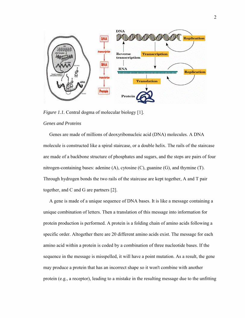
cells and the majority of bio-active molecules. Figure 1.1 shows the central dogma of
molecular biology [1].
The relationships of DNA, RNA, and Proteins are: Proteins determines the activity of
the cells. They are the physical format of the abstract information integrated in the
genome. DNA contains the genetic information and each cell has a copy. It is stable,
packaged, and inert. RNA is the messenger and translator. It is unstable and lacks
secondary structure. Some RNA has enzymatic activity.
2
Figure 1.1. Central dogma of molecular biology [1].
Genes and Proteins
Genes are made of millions of deoxyribonucleic acid (DNA) molecules. A DNA
molecule is constructed like a spiral staircase, or a double helix. The rails of the staircase
are made of a backbone structure of phosphates and sugars, and the steps are pairs of four
nitrogen-containing bases: adenine (A), cytosine (C), guanine (G), and thymine (T).
Through hydrogen bonds the two rails of the staircase are kept together, A and T pair
together, and C and G are partners [2].
A gene is made of a unique sequence of DNA bases. It is like a message containing a
unique combination of letters. Then a translation of this message into information for
protein production is performed. A protein is a folding chain of amino acids following a
specific order. Altogether there are 20 different amino acids exist. The message for each
amino acid within a protein is coded by a combination of three nucleotide bases. If the
sequence in the message is misspelled, it will have a point mutation. As a result, the gene
may produce a protein that has an incorrect shape so it won't combine with another
protein (e.g., a receptor), leading to a mistake in the resulting message due to the unfitting
3
shape. In other words, if the message in the gene is misspelled, the protein it encodes may
be wrong and its function in the body may be changed. In general, experimental and
computational evidence shows that many genes produce an average of three different
proteins and as many as ten protein products. The protein-coding regions of a gene are
called exons, while the non-coding regions are called introns. Due to alternative splicing,
the exons of a gene can be combined in different ways to make variants of the complete
protein [3].
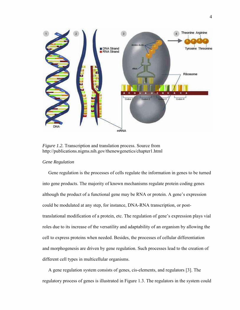
Gene Expression
By using the information from the DNA sequence of a gene, the synthesis of
functional gene products is usually called gene expression. In Figure 1.2, it shows that
there are two major steps in gene expression: transcription of DNA and translation of mRNA
into protein. Here, the products are often proteins or functional RNA. Protein is
considered the most basic building block of life. The roles that proteins play in the
process of life include constituting cell structures, regulating cellular processes,
catalyzing biochemical reactions in metabolic pathways, etc. The specific functions of a
certain protein are determined by its particular physical structure and chemical properties.
Several steps in the gene expression process may be modulated, including the
transcription, RNA splicing, translation, and post-translational modification of a protein.
Gene regulation gives the cell control over structure and function, and is the basis for
cellular differentiation, morphogenesis and the versatility and adaptability of any
organism. Gene regulation may also serve as a substrate for evolutionary change, since
control of the timing, location, and amount of gene expression can have a profound effect
on the functions of the gene in a cell or in a multicellular organism.
4
Figure 1.2. Transcription and translation process. Source from http://publications.nigms.nih.gov/thenewgenetics/chapter1.html
Gene Regulation
Gene regulation is the processes of cells regulate the information in genes to be turned
into gene products. The majority of known mechanisms regulate protein coding genes
although the product of a functional gene may be RNA or protein. A gene’s expression
could be modulated at any step, for instance, DNA-RNA transcription, or post-
translational modification of a protein, etc. The regulation of gene’s expression plays vial
roles due to its increase of the versatility and adaptability of an organism by allowing the
cell to express proteins when needed. Besides, the processes of cellular differentiation
and morphogenesis are driven by gene regulation. Such processes lead to the creation of
different cell types in multicellular organisms.
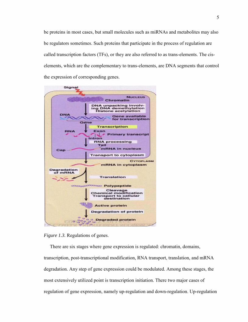
A gene regulation system consists of genes, cis-elements, and regulators [3]. The
regulatory process of genes is illustrated in Figure 1.3. The regulators in the system could
5
be proteins in most cases, but small molecules such as miRNAs and metabolites may also
be regulators sometimes. Such proteins that participate in the process of regulation are
called transcription factors (TFs), or they are also referred to as trans-elements. The cis-
elements, which are the complementary to trans-elements, are DNA segments that control
the expression of corresponding genes.
Figure 1.3. Regulations of genes.
There are six stages where gene expression is regulated: chromatin, domains,
transcription, post-transcriptional modification, RNA transport, translation, and mRNA
degradation. Any step of gene expression could be modulated. Among these stages, the
most extensively utilized point is transcription initiation. There two major cases of
regulation of gene expression, namely up-regulation and down-regulation. Up-regulation
6
occurs within a cell, which results in increased expression of one or more genes while
down-regulation results in decreased gene expression and corresponding protein
expression. The regulation mechanism includes the binding of certain TFs to cis-elements
and then controls the level of target gene’s expression during transcription. A gene’s
expression is regulated by some regulators, while its own expressed products can be
regulators of another gene. The gene regulatory network (GRN) is formed by such
complex regulatory connections [3].
DNA Microarray Technology
Functional genomics involves the analysis of large datasets of information derived
from various biological experiments. One such type of large-scale experiment involves
monitoring the expression levels of thousands genes simultaneously under a particular
condition, called gene expression analysis. Microarray technology makes use of the
sequence resources created by the genome projects and other sequencing efforts to
answer the question, what genes are expressed in a particular cell type of an organism, at
a particular time, under particular conditions.
DNA Microarray
A DNA microarray is a multiplex technology used in molecular biology, which
consists of an arrayed series of thousands of microscopic spots of DNA oligonucleotides,
called features (genes). Each feature contains picomoles (10-12 moles) of a certain DNA
sequence, which are also known as probes. Such probes can be a fragment of a gene or
other DNA element which are used to hybridize with a cDNA/cRNA sample under
experimental designed conditions. A microarray experiment is able to accomplish several
genetic tests in parallel because tens of thousands of probes can be included in an array.
Thus, microarray technology allows us to monitor tens of thousands of gene expressions

7
and have significantly accelerated the investigations of many types of biology
experiments. Figure 1.4 illustrated the overall workflow of a microarray experiment.
Figure 1.4. Workflow of microarray experiment. Source from http://images-mediawiki-sites.thefullwiki.org/06/3/9/3/8878261581107656.png
Microarray technology evolved from Southern blotting, where fragmented DNA is
attached to a substrate and then probed with a known gene or fragment. The use of a
collection of distinct DNAs in arrays for expression profiling was first described in 1987,
and the arrayed DNAs were used to identify genes whose expression is modulated by
interferon [4]. These early gene arrays were made by spotting cDNAs onto filter paper
with a pin-spotting device. The use of miniaturized microarrays for gene expression
profiling was first reported in 1995 [5], and a complete eukaryotic genome on a
microarray was published in 1997 [6].
Microarray Types and Applications
There exist many types of microarrays and they are differed by whether being
spatially arranged on a surface or on coded beads. The early-stage array is a collection of
orderly microscopic spots. Each spot is combined with a specific probe attached to a solid
surface, such as silicon, glass or plastic biochip. The location of a certain probe has been
arranged and thousands of these probes are placed on a single DNA microarray. On the
alternative, bead array is a collection of microscopic polystyrene beads. A specific probe
8
and a ratio of two or more dyes are combined with each bead. Thus, they do not interfere
with the fluorescent dyes used on the target sequence. DNA microarrays technology can
be used in many areas such as gene expression profiling, comparative genomic
hybridization, chromatin immunoprecipitation on Chip (ChIP), SNP detection, alternative
splicing detection [4, 5, 7, 8] and etc.
Microarray Data Analysis
Microarray experiments are inexpensive compare to many other biological
experimental technologies. However, there exist several specific bioinformatics
challenges as follows: first one is the multiple levels of replication in experimental
design. Due to the biological complexity of gene expression, experiment design of a
microarray experiment is critically important if statistically and biologically valid
conclusions need to be elucidated from the data [9]. The second challenge is the number
of platforms and distinct groups and data format. Microarray data is impossible to be
exchanged due to the lack of standard protocols in platform fabrication, assay types, and
analysis approaches. The "MicroArray Quality Control (MAQC) Project" is being
conducted by the US Food and Drug Administration (FDA) to form standards and quality
control metrics which will allow the use of microarray data in many fields such as drug
discovery, clinical practice and regulatory decision-making [10, 11]. The third challenge
is statistical analysis regards to accuracy and precision. Microarray data sets are normally
of huge amount, and its analytical precision is influenced by several variables. Statistical
challenges include effects of image background noise, whether appropriate normalization
and transformation techniques are conducted, identification of significantly differentially
expressed genes (DEGs) [12, 13, 14, 15] as well as inference of gene regulatory networks
9
[16]. How to reduce the dimensionality of microarray dataset in order to obtain more
comprehension and focused analysis requires further preprocess of microarray data [17].
Contributions
In this dissertation, we have made a number of contributions in identification and
optimization of classifier genes and significant pathways. Based on such information,
reconstruction of gene regulatory networks of interested pathways was performed, and all
above work were summarized below.
Identification and Optimization of Classifier Genes
One important goal of microarray experiments is to discover novel classifier genes
which play vital roles in genetic and molecular interactions. Microarrays have been
successfully served as a research tool in discovering novel drug targets [18] and disease-
or toxicity-related biomarker genes for cancer classification [19]. A challenge in
classifying or predicting the diagnostic categories using microarray data is the curse of
dimensionality problem coupled with sparse sampling. That is, the number of examined
genes per sample is much greater than the number of samples that are involved in
classification [20]. The other crucial challenge is that the huge search space for an
optimal combination of classifier genes renders high computational expenses [21]. To
address these two issues, we developed the new Integrated statistical and machine
learning (ISML) pipeline, which integrates statistical analysis with supervised and
unsupervised machine learning techniques. A set of classifier/biomarker genes from high
dimensional datasets were identified and classification models of acceptable precision for
multiple classes were generated as well by our pipeline. More details will be discussed in
Chapter III.
10
Reference Network Builder
Gene Regulatory Networks (GRNs) provide integrated views of gene interactions that
control biological processes. Many public databases contain biological interactions
extracted from literature with experimental validations, but most of them only provide
information for a few genetic model organisms. A number of computational models have
been developed to infer GRN from microarray data, and these models are often evaluated
on model organisms. Researchers who work with non-model organisms rely on these
computational models to build GRN for less-studied organisms. However, they can only
evaluate GRNs built by computational models based on the evaluation criteria such as
recall, precision tested on model organisms. The accuracy and reliability of the tools are
critical for non-model organisms. The researchers also are interested in evaluating the
GRN based on “true” GRN of their organisms. Although, some public network databases
provide experimentally validated interactions among genes or proteins, there are
limitations in accessibility and scalability. Thus, we developed a cyber-based integrated
environment, called "reference network (RefNet)", to build a reference gene regulatory
network for less-studied organisms. The resulting reference network could be used for
validation of inferred GRNs or as prior knowledge for further inference.
Gene Regulatory Network Reconstruction
In the past, many computational models have been proposed to infer gene regulatory
networks. Among them Probabilistic Boolean Network (PBN) [22, 23, 24, 25, 26] and
Dynamic Bayesian Network (DBN) [27, 28, 29, 30, 31] are two popular and powerful
models. PBN is a discrete state space model which characterizes a system using
quantized data, while DBN is an extension of Bayesian network model to incorporate
temporal concept. Previous studies showed that both PBN and DBN approaches had good
11
performance in modeling the gene regulatory network, but DBN identified more gene
interactions and gave better accuracy than PBN [32]. Besides, Zou et al. [28] used DBNs
with various time-delays, by shifting time-series profiles with properly predicted amount
of time steps. Therefore, we used the time-lagged DBN to reconstruct those chemical-
induced networks/pathways which were identified by the RefNet (see Chapter IV) to
analyze the dynamics caused by perturbations.
Dissertation Organization
This dissertation is organized as follows: In Chapter II, we introduce some basic
concepts and backgrounds of microarray experiments and gene regulatory networks.
Then some data preprocessing methods and techniques based on microarray data are
introduced, such as transformation, normalization, etc. We also discuss some statistical
models to identify differentially expressed genes such as t-test, ANOVA and others for
either two-class comparison or multi-class comparison. Then, some machine learning
methods such as clustering, classification based on microarray data for feature selection
and identification of biomarker genes are reviewed.
In Chapter III, we proposed an integrated pipeline combining statistical analysis and
machine learning approaches to identify a set of classifier genes for disease diagnostic
and toxicity evaluation. We assembled an integrated statistical and machine learning
pipeline consisting of several well-established feature filtering/selection and classification
techniques to analyze microarray dataset in order to construct classifier models that can
separate samples into different treatment groups such as evaluating toxicity exposure in
certain environment or diagnosing cancer patients from normal people, etc.
In Chapter IV, a cyber-based environment to retrieve reference genetic interaction
network (RefNet) is proposed. Our RefNet toolbox provides the following services: (1) to
12
build reference GRN/Pathway for non-model organisms; (2) to provide biological prior
knowledge of GRN to improve computational models; (3) to interpret and compare the
GRNs built from computational models with wet-lab experiments; and (4) to serve as a
gene selection tool for GRN reconstruction.
In Chapter V, we introduced and discussed various computational methodologies to
infer gene regulatory network. A review of existing inferring algorithms such as Boolean
networks, Bayesian networks, and Dynamic Bayesian network is given. The time-lagged
dynamic Bayesian network model was used to reconstruct sets of genes from selected
pathways by RefNet. Results showed that our strategy helped with the improvement of
accuracy as well as computational cost of GRN reconstruction and novel biological
knowledge was discovered. In Chapter VI, by integrating all the toolkits and services for
microarray data mining and gene regulatory network analysis, we presented two case
studies to present the detailed contextual analysis.
We complete the dissertation by summarizing our work, and providing sets of issues
appropriate for future work in Chapter VII.
13
CHAPTER II
REVIEW OF MICROARRAY DATA MINING
Microarray Experiments and Data Generation
A microarray experiment requires a number of cDNA or oligonucleotide DNA
sequences (probes) that are affiliated to a glass, nylon, or quartz wafer (adopted from the
semiconductor industry and used by Affymetrix, Inc. [33]). Then material containing
RNA, which is acquired from the biological samples to be studied, is mixed with this
array. For example, the mixture of samples from normal tissues with samples from cancer
tissues. Figure 2.1 illustrates the basic process of cDNA microarray experiments.
Microarrays can be manufactured using various technologies. In spotted microarrays,
the probes are oligonucleotides, cDNA or small fragments of PCR products that
correspond to mRNAs. The probes are synthesized prior to deposition on the array
surface and are then "spotted" onto glass. The resulting grid of probes represents the
nucleic acid profiles of the prepared samples. This provides a relatively low-cost
microarray that may be customized for each study, and avoids the costs of interest to the
investigator. However, publications exist which indicate such microarrays may not
provide the same level of sensitivity compared to commercial oligonucleotide arrays [34].
In oligonucleotide microarrays, the probes are short sequences designed to match parts of
the sequence of known or predicted Expressed Sequence Tags (ESTs), which is a short
sub-sequence of a transcribed cDNA sequence [35]. Oligonucleotide arrays are produced
by printing short oligonucleotide sequences designed to represent a single gene or family
of gene splice-variants by synthesizing this sequence directly onto the array surface
instead of depositing intact sequences. Sequences may be longer (60-mer probes such as
the Agilent design) or shorter (25-mer probes produced by Affymetrix) depending on the

14
desired purpose; longer probes are more specific to individual target genes, shorter
probes may be spotted in higher density across the array [36].
Figure 2.1. Process of cDNA microarray experiment design. Source from http://www.microarray.lu/en/MICROARRAY_Overview.shtml
Two-color microarrays or two-channel microarrays are typically hybridized with
cDNA prepared from two types of samples to be compared (i.e., chemical-treated sample
versus un-treated sample) and they are labeled with two different fluorophores [37]. Cy3
and Cy5 are two common fluorescent dyes that are used for cDNA labeling. The two Cy-
labeled cDNA samples are mixed and hybridized to a single microarray which is then
scanned in a microarray scanner to measure the intensities of fluorescence of the two
fluorophores after excitation with a laser beam of a defined wavelength. Relative
intensities of each fluorophore are then used to identify up-regulated and down-regulated
genes [38]. In single-channel or one-color microarrays, the array provides intensity data
for each probe indicating a relative level of hybridization with the labeled target.

15
However, this intensity data is not true indicator of abundance level of a gene, but rather
a relative abundance when compared with other samples processed in the same
experiment. Since each chip is exposed to only one sample as opposed to two-channel
platform, the single-channel system is more accurate. In one-color array chip, an aberrant
sample cannot affect the raw data derived from other samples. While in two-color array
chip, a single low-quality sample may drastically impinge on the precision of overall data
set even if the other sample was of high quality. Another advantage of single-channel
chip is that it is much easier when comparing data to arrays from different experiments as
long as batch effects are taken care of.
Microarray Data Preprocessing
Image Processing Analysis
The population of mRNA in a certain sample can be stored as an image with intensity
values indicating the relative expression level for each gene. The array chips are scanned
by microarray scanners, which are provided by microarray manufacturers, and the
intensity values of each spot on the chip are recorded. Image processing involves the
following steps: (1) Identification of the spots and distinguishing them from spurious
signals. The microarray is scanned following hybridization and an image file is
generated. Once image generation is completed, the image is then analyzed to identify
spots and used to identify regions that correspond to spots; (2) Determination of the spot
area will be studied and identification of the local region is used to estimate background
noise. After identifying regions that correspond to sub-arrays, in order to get a
measurement of the spot signal and estimated for background intensity, a region within
the sub-array needs to be selected; (3) Reporting statistics summary and generate spot
intensity by subtracting background intensity. In this step, once the center and
16
background areas have been determined, a number of statistics summary for each spot are
reported. Another concern in image processing is the number of pixels to be included for
measurement in the spot image [39
However, it is better to use a smaller pixel size to make sure enough pixels included.
Even though using a smaller pixel size increases the confidence in the measurement, the
image size tends to be bigger when compared with ones using larger pixel size.
Data Normalization and Transformation
The purpose of normalization is to eliminate variations to allow appropriate
comparison of data that is obtained from each sample. Comparison of different
arrays/samples normally involves making adjustments for systematic errors which is
introduced by different procedures and effects. The order of operations for filtering the
data is that spot filters are applied first, then data normalization, and then truncation of
extreme values, then gene screening.
Spot filtering refers to filters on spots in individual arrays. Spot filtering is used for
quality control purposes, i.e., to filter out “bad” spots. Unlike gene screening, Spot
filtering does not filter out the entire gene (a row), but replaces the existing values of a
spot within any given array with a missing value. There exist four types of spot filters:
intensity filter, spot flag filter, spot size filter and detection call filter. The intensity filter
is applied to the background adjustment of signals and different parameters are adopted
for dual-channel or single-channel data. The spot flag filter can contain both numeric and
character values. Outside of a specified numeric range, a flag is considered to be
“excluded”. For example, in Affymetrix array, a Detection Call column is used to
designate as the spot flag at the time of collating, which allows the users to filter out
expression values that have an “A” (Absent) call. Additionally, the spot flag is also used

17
to filter out spots with a large percentage of expression values that have a spot flag value
of “A”.
In general, a logarithmic (base 2) transformation is applied to the signal intensities (for
single-channel data) or intensity-ratios (for dual-channel data) before they are normalized
and truncated. There are currently four major normalization options: median
normalization, housekeeping gene normalization, lowess normalization as well as print-
tip group normalization. The first two are available for both single-channel and dual-
channel data, but the last two are only for dual-channel data. For single-channel data, the
user needs to choose a reference array against which all other arrays will be normalized.
The “median” reference array is selected as following algorithm:
(1) Let N be the number of experiments, and let i be an index of experiments running
from 1 to N.
(2) For each array i, the median log-intensity of the array (denoted Mi) will be
computed.
(3) A median M will be selected from the {M1,…,MN} values. If N is even, then the
median M will be the lower of the two middle values.
(4) The array whose median log-intensity Mi equals the overall median M will be
chosen as the median array.
Then, the median normalization is performed by subtracting out the median log-ration for
each array, so that each normalized array has a median log-ration of 0. Such median
normalization is called per-gene normalization. Besides, per chip normalization is
performed by computing a gene-by-gene difference between each array and the reference
array, and subtracting the median difference from the log-intensities on that array, so that
the gene-by-gene difference between the normalized array and the reference array is 0.

18
Figure 2.2. Intensity distribution of arrays before and after median normalization.
For dual-channel data, locally weighted linear regression (LOWESS) normalization is
normally used. In the lowess normalization, a non-linear lowess smoother function is fit
to the graph of un-normalized log-ratio on the y-axis versus average log intensity (i.e.,
[log(R)+log(G)]/2) on the x-axis. That is, lowess normalization assumes that the dye bias
appears to be dependent on spot intensity. The adjusted ratio is computed by the
following Equation 2.1:
log log ( ) (2.1)where c(A) is the lowess fit to the log / versus log × plot. Lowess regression is
a technique for fitting a smoothing curve to a dataset. The degree of smoothing is
determined by the window width parameter. In general, a larger window width results in
a smoother curve, while a smaller window results in local variation [40, 41, 42, 43].
Figure 2.3 shows the plots under different lowess window width.

19
Figure 2.3. Spot intensity plots with different lowess window width.
Missing Values
After applying various techniques of normalization or filtering, missing expression
values may exists in the data sets. However, many further gene expression analysis
require a complete matrix of array values. Even missing values are allowed for some
analysis algorithms, they are treated as intensity value of zero when calculated, which
will certainly affect the accuracy and validity of analysis results. Therefore, methods for
imputing missing data are needed to minimize the effect of incomplete data sets.
Previously, three most popular methods to impute missing values are proposed, namely,
Singular Value Decomposition (SVD) based method (SVDimpute) [45, 46, 47], weighted
K-nearest neighbors (KNNimpute) [44], as well as row average. The KNN-based method
selects genes whose expression profiles are similar to the gene of interest to impute
missing values. Suppose there is a missing value in experiment 1 for gene A, KNNimpute
will find K other genes whose expression values are most similar to A in experiments 2 to
N. Euclidean distance, which is the metric for gene similarity is used during the imputing
process. The row average technique is trivial as calculating the average of the row
20
containing missing values and filling them with it. SVDimpute method can only be
performed on complete matrices, so row average is imputed for all missing values and
then utilize an expectation maximization method to arrive at the final estimate.
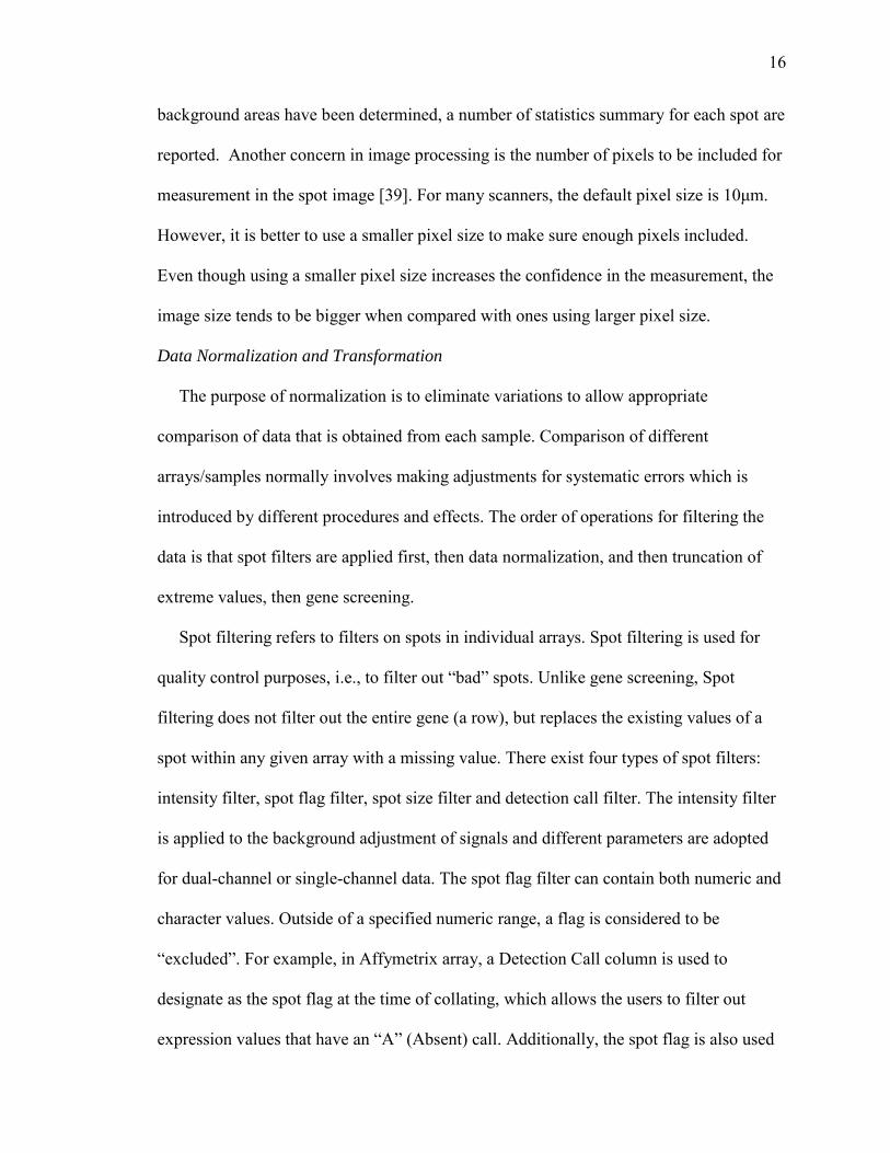
Troyanskaya et al. compared the above three missing value imputation techniques and
KNN-based estimations turned out to have best performance among the three on the same
data set.
Figure 2.4. Comparison of KNN, SVD, and row average based estimations’ performance on the same data set [44].
Identification of Differentially Expressed Genes (DEGs)
One of the common interests of microarray analysis is to identify genes that are
significantly differentially expressed. Such DEGs are ones with expression ratio
significantly different from 1 and are considered as important genes in later analysis
study such as classification, clustering, or gene regulatory network reconstruction.
Although some clustering techniques are used to find groups of genes with similar
patterns [48, 49, 50], it is still very useful to find those genes that are changed
significantly between different samples or conditions. A number of methods are proposed
to identify the largely varied genes such as fold-change cut-off (usually two folds is used)
method or a statistical approach called “Z-score”, which calculates the mean and standard
21
deviation of the distribution of intensity values and defines a global fold change
difference and confidence level. Therefore, if the confidence level is chosen at 95%,
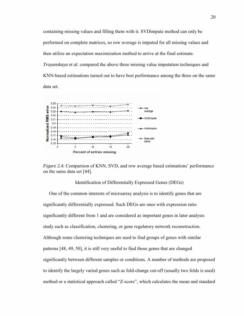
DEGs will have a Z-score value of Z > 1.96 [51]. Figure 2.5 illustrates an example of a Z-
score selection application.
Figure 2.5. Intensity-dependent Z-scores for identifying differential expression.
In general, if two classes are compared and the experiments are paired, the paried t-
test could be used to find DEGs. For example, DEGs can be found by comparing samples
from cancer tissues with normal tissues. Here, either a single replicate for each RNA
sample is used or the averaging mean of all replicates should be used. T-test (or F-test) is
based on the comparison of differences in the mean log-ratios / log-intensities between
classes relative to the variation expected in the mean differences. It is assumed that all the
samples are independent. Alternatively, if multivariate permutation classes need to be
compared (i.e., more than two classes), analysis of variance (ANOVA) is used, usually
one-way ANOVA. The ANOVA test the null hypothesis that samples in multiple groups
are drawn from the same population. Two estimates, which are made of the population
variance, rely on various assumptions such as independent samples, equal variances of

22
populations, etc. The ANOVA calculates an F-score, which is the ratio of the variance
among the means to the variance within the samples.
Feature Selection
Due to the “curse-of-dimensionality,” i.e., the large dimensionality (usually contain
tens of thousands of genes) and their relatively small sample sizes [52], it is of great
challenge to analyze microarray data using data mining techniques. Furthermore,
experimental complications such as systematic noise and variability add more difficulties
to the analysis. Thus, one of the effective ways to deal with these particular
characteristics of microarray data is to reduce the dimension and select “useful” features
[53, 54, 55, 56]. A number of feature selection techniques has been proposed and studied
to contribute to feature selection methodologies [57]. There are two major types of
feature selection methods: univariate filtering and multivariate filtering. Figure 2.6
summarizes the most widely used techniques [58].
Univariate Filtering
Due to the high dimensionality of microarray data set, fast and efficient feature
selection techniques such as univariate filtering methods are widely used. Previously and
nowadays, comparative evaluations of different classification and feature selection
techniques over DNA microarray datasets are normally focused in the univariate cases
[59, 60, 61, 62]. Some trivial heuristics for the identification of DEGs include choosing a
threshold for the fold-change differences in gene expression, and detection of the
threshold point in each gene that minimizes the misclassification of training sample
numbers [63]. Furthermore, new or adapted univariate feature ranking techniques has
been developed, which is divided into two classes: parametric and model-free methods.
Parametric methods assume a given distribution from which the samples have been

23
generated. Among them, t-test and ANOVA are the most widely used approaches in
microarray analysis. Dominating the parametrical analysis field by Gaussian
assumptions, other parametrical approaches such as regression modeling technique [64]
and Gamma distribution models [65] are also useful.
Figure 2.6. Key references for feature selection technique in microarray domain [58].
Multivariate Filter Paradigm
Univariate filtering approaches have specific restrictions and may cause less accurate
classifiers. For example, gene to gene regulatory interactions are not considered.
Therefore, techniques that capture such correlations between genetic interactions are
proposed. The widely used applications of multivariate filter methods includes simple
bivariate interactions [66], correlation-based feature selection (CFS) [67, 68] as well as
some variants of the Markov blanket filter method [69, 70, 71]. An alternative way to
perform a multivariate gene selection is to use wrapper or embedded methods. This could
incorporate the classifier’s bias into the search space and more accurate classifiers might
24
be constructed. Most wrapper approaches use population-based, randomized search
heuristics [72, 73, 74, 75] while others use sequential search techniques [76, 77].
Inference of Gene Regulatory Networks (GRNs)
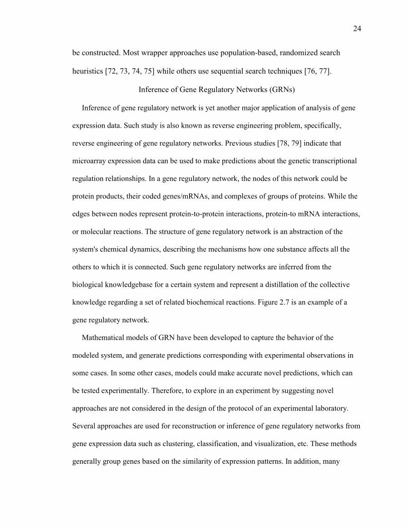
Inference of gene regulatory network is yet another major application of analysis of gene
expression data. Such study is also known as reverse engineering problem, specifically,
reverse engineering of gene regulatory networks. Previous studies [78, 79] indicate that
microarray expression data can be used to make predictions about the genetic transcriptional
regulation relationships. In a gene regulatory network, the nodes of this network could be
protein products, their coded genes/mRNAs, and complexes of groups of proteins. While the
edges between nodes represent protein-to-protein interactions, protein-to mRNA interactions,
or molecular reactions. The structure of gene regulatory network is an abstraction of the
system's chemical dynamics, describing the mechanisms how one substance affects all the
others to which it is connected. Such gene regulatory networks are inferred from the
biological knowledgebase for a certain system and represent a distillation of the collective
knowledge regarding a set of related biochemical reactions. Figure 2.7 is an example of a
gene regulatory network.
Mathematical models of GRN have been developed to capture the behavior of the
modeled system, and generate predictions corresponding with experimental observations in
some cases. In some other cases, models could make accurate novel predictions, which can
be tested experimentally. Therefore, to explore in an experiment by suggesting novel
approaches are not considered in the design of the protocol of an experimental laboratory.
Several approaches are used for reconstruction or inference of gene regulatory networks from
gene expression data such as clustering, classification, and visualization, etc. These methods
generally group genes based on the similarity of expression patterns. In addition, many
25
Figure 2.7. A typical gene regulatory network. Source from http://upload.wikimedia.org/wikipedia/commons/thumb/c/c4/Gene_Regulatory_Network.jpg/360px-Gene_Regulatory_Network.jpg
computational approaches have been proposed to reconstruct gene regulatory networks based
on large-scale microarray data retrieved from biological experiments such as information
theory [80, 81, 82, 83, 84], Boolean networks [23, 26, 85, 86, 87, 88], differential equations
[89, 90, 91, 92, 93], Bayesian networks [27, 28, 29, 30, 94, 95, 96] and neural networks [97].
Many computational methods have been developed for modeling or simulating GRNs.

26
CHAPTER III
IDENTIFY CLASSIFIER GENES USING ISML PIPELINE
From a regulatory standpoint, there is an increasing and continuous demand for more
rapid, more accurate and more predictive assays due to the already large but still growing,
number of man-made chemicals released into the environment [98]. Molecular endpoints
such as gene expression that may reflect phenotypic disease symptoms manifested later at
higher biological levels (e.g., cell, tissue, organ, or organism) are potentially biomarkers
that meet such demands. As a high throughput tool, microarrays simultaneously measure
thousands of biologically-relevant endpoints (gene expression). However, to apply this
tool to animals under field conditions, one critical hurdle to overcome is the separation of
toxicity-induced signals from background noise associated with environmental variation
and other confounding factors such as animal age, genetic make-up, physiological state
and exposure length and route [99, 100]. A common approach to biomarker discovery is
to screen genome- or transcriptome-wide gene expression responses and identify a small
subset of genes capable of discriminating animals that received different treatments, or
predicting the class of unknown samples. It is relatively less challenging to identify
differentially expressed genes from two or more classes of samples. However, the search
for an optimal and small subset of genes that has a high discriminatory power in
classifying field samples often having multiple classes is much more complicated.
We propose an integrated statistics and machine learning (ISML) pipeline to analyze
the microarray dataset in order to construct classifier models that can separate samples
into different chemical treatment groups. The results show that our approach can be used
to identify and optimize a small subset of classifier/biomarker genes from high
27
dimensional datasets and generate classification models of acceptable precision from
multiple classes.
Integrated Statistical and Machine Learning (ISML) Pipeline
Overview of ISML
A challenge in classifying or predicting the diagnostic categories using microarray
data is the curse of dimensionality problem coupled with sparse sampling. That is, the
number of examined genes per sample is much greater than the number of samples that
are involved in classification [101]. The other crucial challenge is that the huge search
space for an optimal combination of classifier genes renders high computational expenses
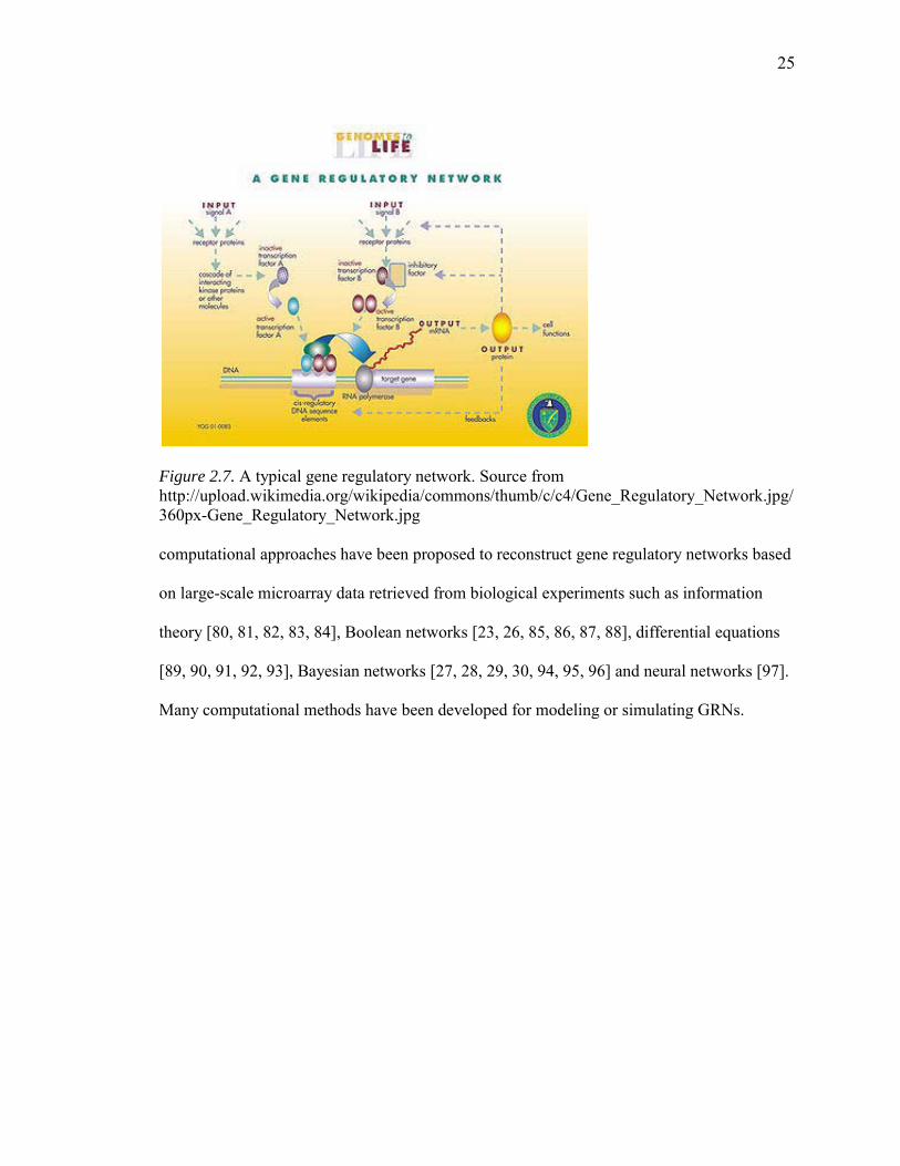
[102]. To address these two issues, we developed the new ISML pipeline, which
integrates statistical analysis with supervised and unsupervised machine learning
techniques (Figure 3.1). The pipeline consists of four major components: (1) statistical
analysis that reduces dimensionality through identification of the most differentially
expressed genes; (2) tree-based algorithms that are used to further downsize the number
of classifier genes with assigned weight and associated ranking; (3) MC-SVM and
unsupervised clustering, each of which independently selects an optimal set of classifier
genes using an iterative elimination process; and (4) the integration of the two
independent gene sets to generate a final refined gene sets.

28
Figure 3.1. Overview of the ISML pipeline.
Feature Filtering by Statistical Analysis
Data Preprocessing
The following data pre-treatment steps were applied prior to further statistical and
computational analyses: (1) feature filtering: flag out spots with signal intensity outside
the linear range as well as non-uniform spots; (2) conversion: convert signal intensity into
relative RNA concentration based on the linear standard curve of spike-in RNAs; (3)

29
normalization: normalize the relative RNA concentration to the median value on each
array; and (4) gene filtering: filter out genes appearing in less than 50% of arrays.
Identification of Differentially Expressed Genes
The Class Comparison Between Groups of Arrays Tool in BRB-ArrayTools v.3.8
software package ([103]; linus.nci.nih.gov/BRB-ArrayTools.html) was used to identify
significantly changed genes. The dataset was normalized and transformed previously, and
then was imported into the BRB-ArrayTools application. The tool runs a random
variance version of the t-test or F-test separately for each gene. It performs random
permutations of the class labels and computes the proportion of the random permutations
that give as many genes significant at the level set by the user as are found in comparing
the true class labels. Differentially expressed genes were inferred by univariate statistical
analysis. In general, we use a univariate test random variance model, multivariate
permutation test with 10,000 random permutations, a confidence level of false discovery
rate assessment = 99%, and a maximum allowed number of false-positive genes = 10.
Classifier Gene Selection and Ranking
Molecular endpoints such as gene expression that may reflect phenotypic disease
symptoms manifested later at higher biological levels (e.g., cell, tissue, organ, or
organism) are potentially biomarkers that meet such demands. As a high throughput tool,
microarrays simultaneously measure thousands of biologically-relevant endpoints (gene
expression). However, to apply this tool to animals under field conditions, one critical
hurdle to overcome is the separation of toxicity-induced signals from background noise
associated with environmental variation and other confounding factors such as animal
age, genetic make-up, physiological state and exposure length and route [99, 100]. A
common approach to biomarker discovery is to screen genome- or transcriptome-wide
30
gene expression responses and identify a small subset of genes capable of discriminating
animals that received different treatments, or predicting the class of unknown samples. It
is relatively less challenging to identify differentially expressed genes from two or more
classes of samples. However, the search for an optimal and small subset of genes that has
a high discriminatory power in classifying field samples often having multiple classes is
much more complicated.
Classifier Gene Selection by Tree-Based Algorithms
A tree structure consists of a number of branches, one root, a number of internal nodes
and a number of leaves. A decision tree is a decision support tool that uses a tree-like
model of decisions and their possible consequences, where each internal node (non-leaf
node) denotes a test on an attribute, each branch represents an outcome of the test, and
each leaf node holds a class label. The topmost node in a tree is the root node. The
occurrence of a node (feature/gene) in a tree provides the information about the
importance of the associated feature/gene. At each decision node in a decision tree, one
can select the most useful feature for classification using estimation criteria such as the
concepts of entropy reduction and information gain. In a decision tree, the feature in the
root is the best one for classification. The other features in the decision tree nodes appear
in descending order of importance, which contribute to the classification, appear in the
decision tree. The features that have less capability of discrimination are discarded during
the tree construction. Thus, the decision tree algorithms could identify good features for
the purpose of classification from the given training dataset.
Seven decision tree methods (SimpleCart, BFTree, FT, J48, LADTree, LMT and
REPTree) were used for gene selection to avoid the biases and overcome limitations of
each single algorithm [105, 106]. An ensemble strategy was also applied to increase
31
prediction accuracy using bagging (Bagging) and boosting (AdaBoostM1) [106]. These
two well known methods are used to construct ensemble by re-sampling techniques.
Bagging builds bags of the same size of the original data set by applying random
sampling with replacement. While boosting resample original data set with replacement,
but weights has been assigned to each training sample. The weights are updated
iteratively to train subsequent classifier to pay more attention to misclassified samples.
The last classifier combines the votes of each individual classifier.
All of these algorithms are implemented in the WEKA machine learning workbench
v.3.6.0 ([108]; www.cs.waikato.ac.nz/ml/weka/). Table 3.1 summarizes the seven tree-
based classification algorithms that were examined and the last two strategies were the
ensemble ones. Each algorithm generated a set of classification rules and a selection of
classifier genes. For each algorithm, a 10-fold cross validation method was used to
calculate the accuracy of the classifiers.
The performance of the classification algorithms was evaluated based on three criteria:
accuracy, Receiver Operating Characteristic (ROC) area, and size of the tree. Accuracy
of a classifier M is the percentage of dataset that are correctly classified by the model M.
ROC Area is the area under the ROC curve, which can be interpreted as the probability
that the classifier ranks a randomly chosen positive instance above a randomly chosen
negative one. Roughly speaking, the larger the area is, the better the model would be. The
ROC can also be represented equivalently by plotting the fraction of true positives (TPR
= true positive rate) versus the fraction of false positives (FPR = false positive rate). The
ROC curve is a comparison of two operating characteristics (TPR & FPR) as the criterion
changes [108].
32
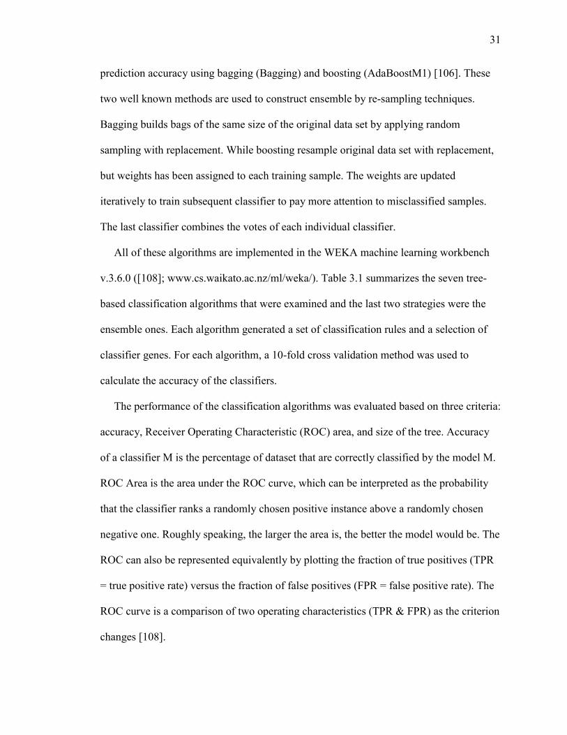
Table 3.1
Tree-Based Classifier Algorithms in WEKA [17]
Classifier Name Function
SimpleCart Class implementing minimal cost-complexity pruning
BFTree Class for building a best-first decision tree classifier
FT Classifier for building “Functional trees” with logistic regression functions at inner nodes/leaves
J48 Class for generating a pruned or un-pruned C4.5 decision tree
LADTree Class for generating a multi-class alternating decision tree using the LogitBoost strategy
LMT Classifier for building 'logistic model trees' with logistic regression functions at the leaves
REPTree Fast decision tree learner
Bagging(ensemble)
Class for bagging a classifier to reduce variance
AdaBoostM1(ensemble)
Class for boosting a nominal class classifier using the Adaboost M1 method
ROC analysis provides tools to select optimal models and is related in a direct and natural
way to cost/benefit analysis of diagnostic decision making. The size of the tree represents
the number of selected genes in an assembled tree. Classification rules generated by
algorithms with ensemble strategy included multiple trees and the total number of non-
redundant classifier genes was counted as the tree size.
Ranking Classifier Genes by Weight of Significance
A weight of significance was assigned on a scale between 0 and 1 to every selected
classifier gene based on its position/significance in an assembled decision tree according
to Equation 3.1:
( ) = max 1_ (3.1)
33
where ( ) is the weight of gene assigned by a tree model t, _ is the longest
path of the tree, and is the height of the gene in path . A “root” gene was awarded the
largest weight whereas a “leaf” gene the smallest. The weight value was normalized to
the longest leaf-to-root path, except for those genes selected by the LMT algorithm,
whose weight had already been assigned by a logistic model. The overall weight for a
classifier gene, i.e., the sum of its weight assigned in all the decision tree methods, was
calculated in Equation 3.2:
( ) = ( ) (3.2)where ( ) is the overall weight of gene , is the accuracy of tree model t, and N is
the total number of tree models. All of the classifier genes were ranked by their overall
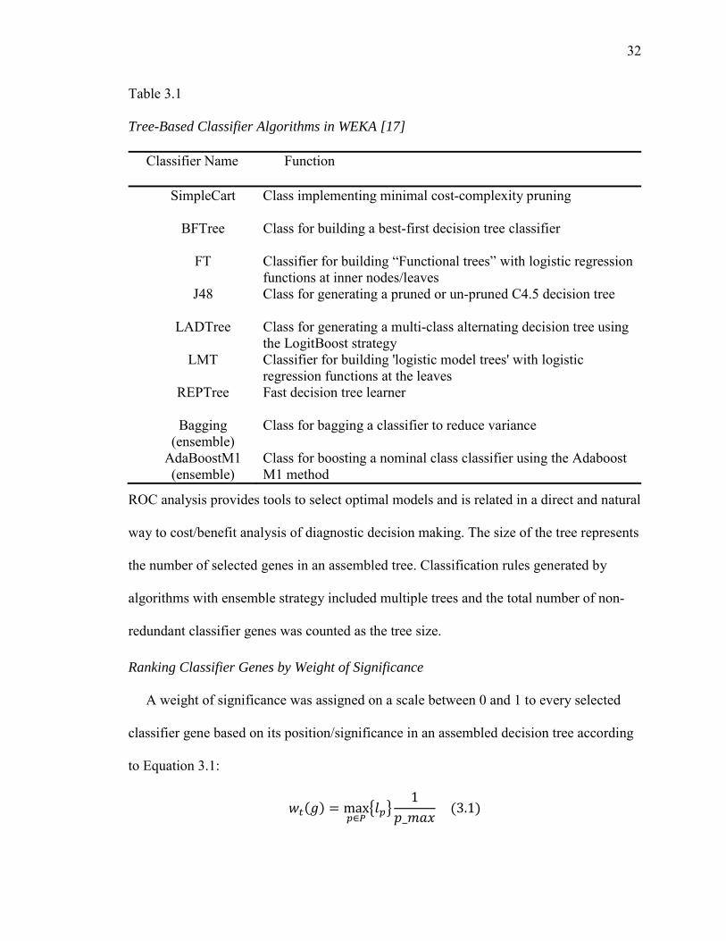
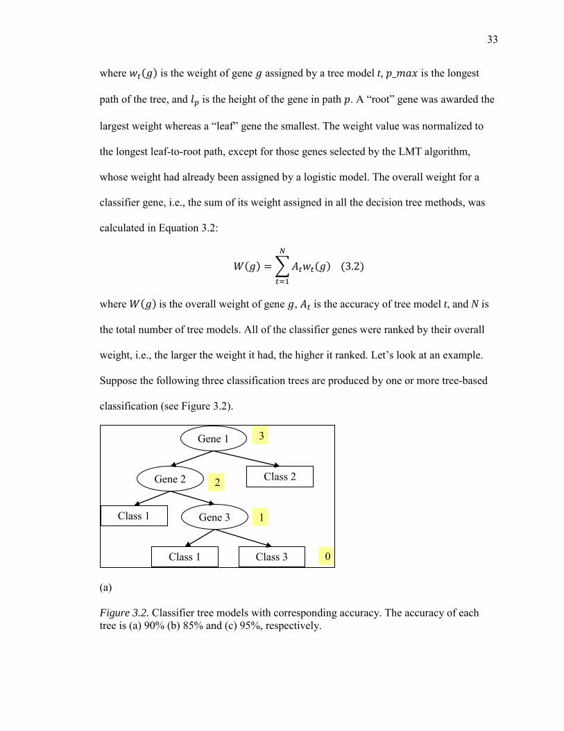
weight, i.e., the larger the weight it had, the higher it ranked. Let’s look at an example.
Suppose the following three classification trees are produced by one or more tree-based
classification (see Figure 3.2).
(a)
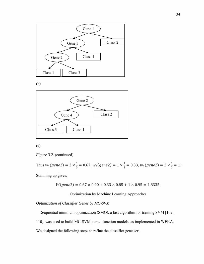
Figure 3.2. Classifier tree models with corresponding accuracy. The accuracy of each tree is (a) 90% (b) 85% and (c) 95%, respectively.
Gene 3
Gene 2
Gene 1
Class 1
Class 2
Class 1 Class 3
1
0
2
3
34
(b)
(c)
Figure 3.2. (continued).
Thus ( 2) = 2 × = 0.67, ( 2) = 1 × = 0.33, ( 2) = 2 × = 1.
Summing up gives:( 2) = 0.67 × 0.90 + 0.33 × 0.85 + 1 × 0.95 = 1.8335.
Optimization by Machine Learning Approaches
Optimization of Classifier Genes by MC-SVM
Sequential minimum optimization (SMO), a fast algorithm for training SVM [109,
110], was used to build MC-SVM kernel function models, as implemented in WEKA.
We designed the following steps to refine the classifier gene set:
Gene 4
Gene 2
Class 1
Class 2
Class 3
Gene 2
Gene 3
Gene 1
Class 1
Class 2
Class 1 Class 3

35
(1) start with the highest ranking classifier gene to train the SVM using the training
dataset and classify the testing dataset using the trained SVM;
(2) add one gene of immediately lower ranking in overall weight at a time to
constitute a new gene set, and use the gene set to train and predict the samples;
repeat this step until all the classifier genes have been included;
(3) calculate the classification accuracy of each class (control, TNT and RDX) and
the weighted average accuracy of all three classes for each set of genes using
results from the testing dataset;
(4) estimate the improvement or decline in classification accuracy as a result of
adding one gene for each of the three classes plus the weighted average accuracy
of all three classes;
(5) remove any gene(s) starting from the one ranking at the bottom that causes a
decline in ALL four classification accuracies; and
(6) Iterate steps 1~5 until no more gene(s) can be removed. The remaining set of
genes is considered the refined classifier gene set because of its small gene size
and high accuracy.
Optimization of Classifier Genes by Clustering
Because both tree-based algorithms and SVM are supervised machine learning
methods, an unsupervised clustering method was used to independently optimize the
classifier genes. Clustering was performed using the K-mean clustering analysis as
implemented in the WEKA toolbox. All the dendrogram trees were cut at a level so that
all the 248 earthworm RNA samples were grouped into three clusters. The three pre-
labelled clusters (control, RDX and TNT) served as the reference, and the three clusters
derived from the dendrogram trees were compared to the reference clusters to determine
36
matching sample numbers. The optimization of classifier genes by clustering followed
the same iterative steps as described above for MC-SVM.
Estimation of Classification Accuracy
Accuracy (also called true positive rate or recall) of a classifier was defined as the
percentage of the dataset correctly classified by the method, i.e., number of correctly
classified samples/total number of samples in the class. Due to the use of the whole
dataset in feature selection, ten-fold stratified cross-validation with inner and outer loops
was performed as described in [111] throughout this study to avoid sample selection bias
and obtain unbiased estimates of prediction accuracies [112].
Identification of Significant Pathways
By using the ISML pipeline, we are able to reduce the dimensionality of microarray
datasets, identify and rank classifier genes, and generate a small set of classifier genes.
However, from the system biology point of view, networks/pathways of genetic
regulation were able to discover the mechanisms of the modern biomedical research.
Thus, having the list of classifier genes which are significant affected by treated chemical
compounds, we are able to identify those relevant highly affected pathways. Combined
with the reference network tool, which was introduced in the next chapter, all the
pathways that includes the classifier genes were selected and ranked based on the number
of classifier genes involved. The resulting ordered list of highly affected pathways are
considered as the candidates for detailed analysis.
37
CHAPTER IV
REFNET: A TOOLBOX TO RETRIEVE REFERENCE NETWORK
Once a list of significant classifier genes has been obtained, the next consideration is
the identification of the biological processes represented in the list. The information
associated with a particular gene, such as the annotation and the relevant biological
interactions, is available from many online resources [114, 115, 116, 117]. Many public
databases contain genetic interactions retrieved from literature with wet-lab experimental
validations. Unfortunately, only a few well-studied model organisms are curated and their
GRN/Pathways are available in most of these public databases. A number of
computational models also have been developed to infer gene regulatory network such as
Boolean Network (BN [23, 26, 85]), Probabilistic Boolean Network (PBN [86, 87, 88]),
Dynamic Bayesian Network (DBN [27, 28, 29, 30, 94, 95, 96]), etc. Such models are
only assessed based on the evaluation criteria such as recall and precision tested on model
organisms. However, researchers who work with non-model organisms also need to
obtain genetic interaction information and use it to systematically analyze their own
organisms. And they rely on these computational models to infer GRN and investigate
the genetic interaction among thousands of genes for less-studied organisms. Due to the
lack of "true" genetic interaction network as reference to assess the reconstructed GRNs,
accuracy and reliability are the critical limitations of using the computational models
which are only evaluated on model organisms for inference of GRNs for non-model
organisms. Although some public network databases provide experimentally validated
interactions among genes or proteins, limitations in accessibility and scalability make it
difficult to extract relevant information for researchers.
38
Several bioinformatics toolkits have been developed to extract biological interactions
from public databases for known interactions of well-studied organism. For example,
BioNetBiulder [119, 120] and NetMatch [122] are Cytoscape [118] plug-ins for
retrieving, integrating, visualization and analysis of known biology networks. However,
their usage is very limited for species whose networks are unknown. Other tools such as
BlastPath [124] and OmicViZ [121], also are Cytoscape [118] plug-ins, provide network
mapping across species based on homology. But they only map query species to its
related model organism; and have limited number of query genes / proteins. For less-
studied organisms, their related species may not be well-annotated. Moreover,
information from a single model organism is usually not enough to map network for
query species. In addition, biological interactions among genes/proteins in an entire
pathway may be more comprehensive than those among several random genes/proteins.
To the best of our knowledge, currently no tools are available that provide an integrated
environment for less-studied non-model organisms GRN. Thus, we propose to develop a
cyber-based reference GRN analysis platform in order to (1) build reference
GRNs/Pathways for non-model organisms; (2) provide biological prior knowledge of
GRN which is useful for improving those computational models; (3) interpret and
compare the GRNs built from computational models with wet-lab experiments; and (4)
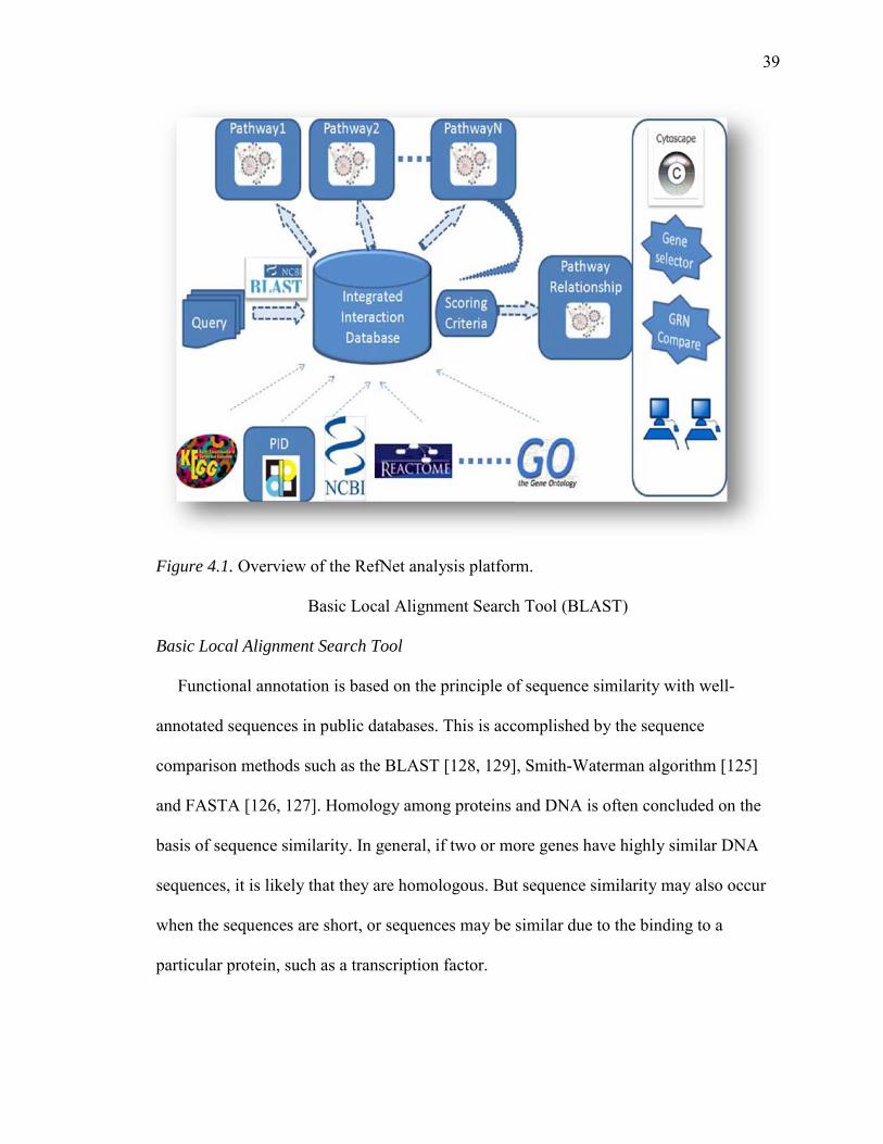
serve as a gene selection tool for GRN reconstruction. Figure 4.1 shows the overall
workflow for the cyber-based RefNet analysis platform.
39
Figure 4.1. Overview of the RefNet analysis platform.
Basic Local Alignment Search Tool (BLAST)
Basic Local Alignment Search Tool
Functional annotation is based on the principle of sequence similarity with well-
annotated sequences in public databases. This is accomplished by the sequence
comparison methods such as the BLAST [128, 129], Smith-Waterman algorithm [125]
and FASTA [126, 127]. Homology among proteins and DNA is often concluded on the
basis of sequence similarity. In general, if two or more genes have highly similar DNA
sequences, it is likely that they are homologous. But sequence similarity may also occur
when the sequences are short, or sequences may be similar due to the binding to a
particular protein, such as a transcription factor.

40
Basic Local Alignment Search Tool (BLAST) [128, 129] is one of the most popular
and widely-used algorithm for comparing primary biological sequence information, such
as the amino-acid sequences of different proteins or the nucleotides of DNA sequences. A
BLAST search enables the comparison of a query sequence with a library or database of
sequences. The library sequences that resemble the query sequence above a certain
threshold will be identified. BLAST is implemented based on the Smith-Waterman
Algorithm, but it emphasizes speed over sensitivity, which makes it more practical on the
huge genome databases currently available. However, BLAST cannot guarantee the
optimal alignments of a certain query sequence with database sequences.
Alignment Theory: Smith-Waterman Algorithm
Before BLAST, alignment programs used dynamic programming algorithms, such as
the Needleman-Wunsch [130] and Smith-Waterman [125] algorithms, that required long
processing times and the use of a supercomputer or parallel computer processors. Both
algorithms are dynamic programming algorithms, but the main difference is that S-W
algorithm sets the negative scoring matrix cells to zero, which renders the local
alignments visible. Backtracking starts at the highest scoring matrix cell and proceeds
until a cell with score zero is encountered, yielding the highest scoring local alignment.
Given a query sequence am and database B, where . Sequence a, b contains m
and n nucleotides respectively. A matrix H is built as in Equation 4.1 and 4.2:( , 0) = 0, 0 (4.1)(0, ) = 0,0 (4.2)if ai = bj w(ai,bj) = w(match) or if ai! = bj w(ai,bj) = w(mismatch)

41
( , ) = 0( 1, 1 + ( , )( 1, ) + ( , )( , 1) + , , 1 , 1 (4.3)where:
a,b = Strings over the
m = length(a)
n = length(b)
H(i,j) - is the maximum Similarity-Score between a suffix of a[1...i] and a suffix of
b[1...j]( , ), , {‘ ’}, where ‘-’ is the gap-scoring scheme
For example, suppose we have sequence a = ACACACTA and sequence b =
AGCACACA. We assign w (match) = +2, w (a, -) = w (-, b) = w (mismatch) = -1.
The resulting matrix H will be obtained and by tracing back, sequence a and b was
aligned as follows:
Configurations of BLAST Program
BLAST increases the speed of alignment by decreasing the search space or number of
comparisons it makes. A word list from the query sequence with words of a specific
length is created and a short "word" (w) segments is used to create alignment "seeds."
Once an alignment is seeded, BLAST extends the alignment according to a threshold (T)
which is set by the user. When performing a BLAST query, the computer extends words
with a neighborhood score greater than T. A cutoff score (S) is used to select alignments
Sequence a = A-CACACTA
Sequence b = AGCACAC-A
42
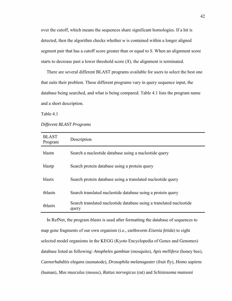
over the cutoff, which means the sequences share significant homologies. If a hit is
detected, then the algorithm checks whether w is contained within a longer aligned
segment pair that has a cutoff score greater than or equal to S. When an alignment score
starts to decrease past a lower threshold score (X), the alignment is terminated.
There are several different BLAST programs available for users to select the best one
that suits their problem. These different programs vary in query sequence input, the
database being searched, and what is being compared. Table 4.1 lists the program name
and a short description.
Table 4.1
Different BLAST Programs
BLAST Program Description
blastn Search a nucleotide database using a nucleotide query
blastp Search protein database using a protein query
blastx Search protein database using a translated nucleotide query
tblastn Search translated nucleotide database using a protein query
tblastx Search translated nucleotide database using a translated nucleotidequery
In RefNet, the program blastx is used after formatting the database of sequences to
map gene fragments of our own organism (i.e., earthworm Eisenia fetida) to eight
selected model organisms in the KEGG (Kyoto Encyclopedia of Genes and Genomes)
database listed as following: Anopheles gambiae (mosquito), Apis mellifera (honey bee),
Caenorhabditis elegans (nematode), Drosophila melanogaster (fruit fly), Homo sapiens
(human), Mus musculus (mouse), Rattus norvegicus (rat) and Schistosoma mansoni
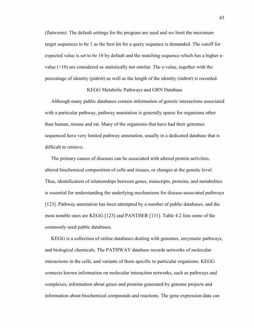
43
(flatworm). The default settings for the program are used and we limit the maximum
target sequences to be 1 as the best hit for a query sequence is demanded. The cutoff for
expected value is set to be 10 by default and the matching sequence which has a higher e-
value (>10) are considered as statistically not similar. The e-value, together with the
percentage of identity (pident) as well as the length of the identity (nident) is recorded.
KEGG Metabolic Pathways and GRN Database
Although many public databases contain information of genetic interactions associated
with a particular pathway, pathway annotation is generally sparse for organisms other
than human, mouse and rat. Many of the organisms that have had their genomes
sequenced have very limited pathway annotation, usually in a dedicated database that is
difficult to retrieve.
The primary causes of diseases can be associated with altered protein activities,
altered biochemical composition of cells and tissues, or changes at the genetic level.
Thus, identification of relationships between genes, transcripts, proteins, and metabolites
is essential for understanding the underlying mechanisms for disease-associated pathways
[123]. Pathway annotation has been attempted by a number of public databases, and the
most notable ones are KEGG [123] and PANTHER [131]. Table 4.2 lists some of the
commonly used public databases.
KEGG is a collection of online databases dealing with genomes, enzymatic pathways,
and biological chemicals. The PATHWAY database records networks of molecular
interactions in the cells, and variants of them specific to particular organisms. KEGG
connects known information on molecular interaction networks, such as pathways and
complexes, information about genes and proteins generated by genome projects and
information about biochemical compounds and reactions. The gene expression data can
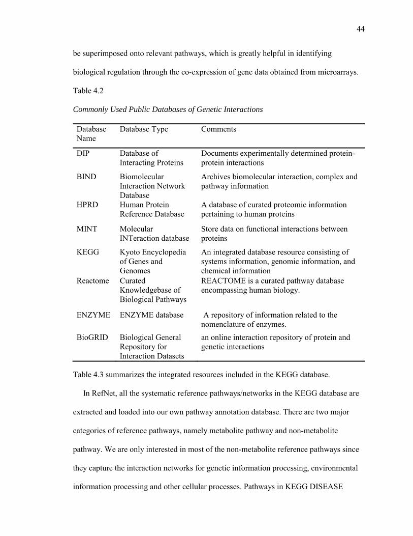
44
be superimposed onto relevant pathways, which is greatly helpful in identifying
biological regulation through the co-expression of gene data obtained from microarrays.
Table 4.2
Commonly Used Public Databases of Genetic Interactions
Database Name
Database Type Comments
DIP Database of Interacting Proteins
Documents experimentally determined protein-protein interactions
BIND Biomolecular Interaction Network Database
Archives biomolecular interaction, complex and pathway information
HPRD Human Protein Reference Database
A database of curated proteomic information pertaining to human proteins
MINT Molecular INTeraction database
Store data on functional interactions between proteins
KEGG Kyoto Encyclopedia of Genes and Genomes
An integrated database resource consisting of systems information, genomic information, and chemical information
Reactome Curated Knowledgebase of Biological Pathways
REACTOME is a curated pathway database encompassing human biology.
ENZYME ENZYME database A repository of information related to the nomenclature of enzymes.
BioGRID Biological General Repository for Interaction Datasets
an online interaction repository of protein and genetic interactions
Table 4.3 summarizes the integrated resources included in the KEGG database.
In RefNet, all the systematic reference pathways/networks in the KEGG database are
extracted and loaded into our own pathway annotation database. There are two major
categories of reference pathways, namely metabolite pathway and non-metabolite
pathway. We are only interested in most of the non-metabolite reference pathways since
they capture the interaction networks for genetic information processing, environmental
information processing and other cellular processes. Pathways in KEGG DISEASE
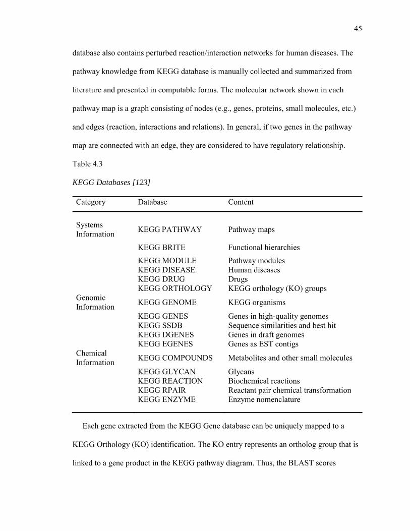
45
database also contains perturbed reaction/interaction networks for human diseases. The
pathway knowledge from KEGG database is manually collected and summarized from
literature and presented in computable forms. The molecular network shown in each
pathway map is a graph consisting of nodes (e.g., genes, proteins, small molecules, etc.)
and edges (reaction, interactions and relations). In general, if two genes in the pathway
map are connected with an edge, they are considered to have regulatory relationship.
Table 4.3
KEGG Databases [123]
Category Database Content
Systems Information KEGG PATHWAY Pathway maps
KEGG BRITE Functional hierarchies
KEGG MODULE Pathway modulesKEGG DISEASE Human diseasesKEGG DRUG DrugsKEGG ORTHOLOGY KEGG orthology (KO) groups
Genomic Information KEGG GENOME KEGG organisms
KEGG GENES Genes in high-quality genomesKEGG SSDB Sequence similarities and best hitKEGG DGENES Genes in draft genomesKEGG EGENES Genes as EST contigs
Chemical Information KEGG COMPOUNDS Metabolites and other small molecules
KEGG GLYCAN GlycansKEGG REACTION Biochemical reactionsKEGG RPAIR Reactant pair chemical transformationKEGG ENZYME Enzyme nomenclature
Each gene extracted from the KEGG Gene database can be uniquely mapped to a
KEGG Orthology (KO) identification. The KO entry represents an ortholog group that is
linked to a gene product in the KEGG pathway diagram. Thus, the BLAST scores

46
between a query sequence and the reference sequence set from the KEGG GENES
database are computed, and homologs are found in the reference set.
RefNet: Reference Network for Non-Model Organisms
After BLAST between query gene and the reference gene set from KEGG GENES
database, homologs are found for each query sequence. Then, homologs ranked above the
threshold are selected as ortholog candidates based on the BLAST score. Ortholog
candidates are divided into KO groups according to the annotation of the KEGG GENES
database and each query sequence was mapped with the corresponding KO group. Figure
4.2 shows the flow chart of RefNet pipeline.
Figure 4.2. Overall procedure of RefNet.
Interpretation of Retrieved Reference Network
The KEGG represents the metabolic and regulatory processes in the form of wiring
diagrams, which can be used for browsing and information retrieval as well as a base for
modeling and simulation. And it helps in understanding biological processes and higher-
order functions of biological systems. Currently the KEGG website uses semi-static
47
visualizations for the presentation and navigation of its pathway information. However, it
does not provide the possibilities of dynamic visualizations or customized visualization
of user-specific pathways. The KEGG system provides a XML representation of its
pathway information called KGML (KEGG Markup Language). Several applications that
support KGML are available for the visualization, analysis and modeling of the
biological networks such as KGML-ED [132], VisANT [133, 134], kegg2sbml,
Biopathways Workbench etc. Not only interactive visualization and exploration of
pathways is desirable to study biological processes, but scientists would also like to
change the pathway structure as to customize interpretation of the pathway. The KGML
visualization and editing tool (KGML-ED) application is a visual exploration method in a
Java based graphical editor. It is based on Gravisto [135], a graph editor and visualization
system, and supports KGML file import and export, visualization and editing of pathway
structures and attributes consistent to the KGML pathway model.
Based on the results of mapping between query sequence and KO reference genes
from the KEGG GENE database, all the reference pathways that are extracted from the
KEGG database were interpreted as highlighting those KO reference genes if they could
be mapped to a query sequence from our own organism. That is, for each pathway map,
the node (representation of ortholog gene) is marked “red” if it is the best hit of a query
sequence from our organism and the gene names are replaced by its corresponding KO
group identification. The rest of the structure on the map remains the same as the original
map from KEGG database. By using the KGML-ED tool, the customized interpretation
of pathway maps, which include mapping information of query gene and KO reference
gene, are generated and can be used as graphical representation of reference network for
reconstruction of GRNs/Pathways for our own non-model organism.
48
CHAPTER V
GENE REGULATORY NETWORK RECONSTRUCTION
Inference of gene regulatory network is yet another major application of analysis of
gene expression data. Such study is also known as reverse engineering problem,
specifically, reverse engineering of gene regulatory networks. Previous studies [78, 79]
indicate that microarray expression data can be used to make predictions about the
genetic transcriptional regulation relationships. In a gene regulatory network, the nodes
of this network could be protein products, their coded genes/mRNAs, and complexes of
groups of proteins. While the edges between nodes represent protein-to-protein
interactions, protein-to mRNA interactions, or molecular reactions. The structure of gene
regulatory network is an abstraction of the system's chemical dynamics, describing the
mechanisms how one substance affects all the others to which it is connected. Such gene
regulatory networks are inferred from the biological knowledgebase for a certain system
and represent a distillation of the collective knowledge regarding a set of related
biochemical reactions.
Mathematical models of GRN have been developed to capture the behavior of the
modeled system, and generate predictions corresponding with experimental observations
in some cases. In some other cases, models could make accurate novel predictions, which
can be tested experimentally. Several approaches are used for reconstruction or inference
of gene regulatory networks from gene expression data such as clustering, classification,
and visualization, etc. These methods generally group genes based on the similarity of
expression patterns. In addition, many computational approaches have been proposed to
reconstruct gene regulatory networks based on large-scale microarray data retrieved from
biological experiments such as information theory [80, 81, 82, 83, 84], Boolean networks
49
[23, 26, 85, 86, 87, 88], differential equations [89, 90, 91, 92, 93], Bayesian networks [27,
28, 29, 30, 94, 95, 96] and neural networks [97]. Many computational methods have been
developed for modeling or simulating GRNs. In this chapter, we reviewed several
widely-used gene regulatory network reconstruction methods, which provide a guideline
to choosing the most appropriate methods to infer the GRNS in a case study described in
Chapter VI.
Information Theory
Information theoretic approaches use a generalization of pairwise correlation
coefficient in Equation 5.1, called Mutual Information (MI), to compare expression
profiles from a set of microarrays. For each pair of genes, their MIij is computed and the
edge aij=aji is set to 0 or 1 depending on a significance threshold to which MIij is
compared. MI can be used to measure the degree of independence between two genes.
= ( ( ) ( ))( ( ) x (k)) (5.1)Mutual information, MIij, between gene i and gene j is computed as in Equation 5.2:MI = + (5.2)where H, the entropy, is defined as in Equation 5.3:
H = (x ) log (x ) (5.3)The entropy Hi has many interesting properties; specifically, it reaches a maximum for
uniformly distributed variables, that is, the higher the entropy, the more randomly
distributed are gene expression levels across the experiments. From the definition, it
follows that MI becomes zero if the two variables xi and xj are statistically independent
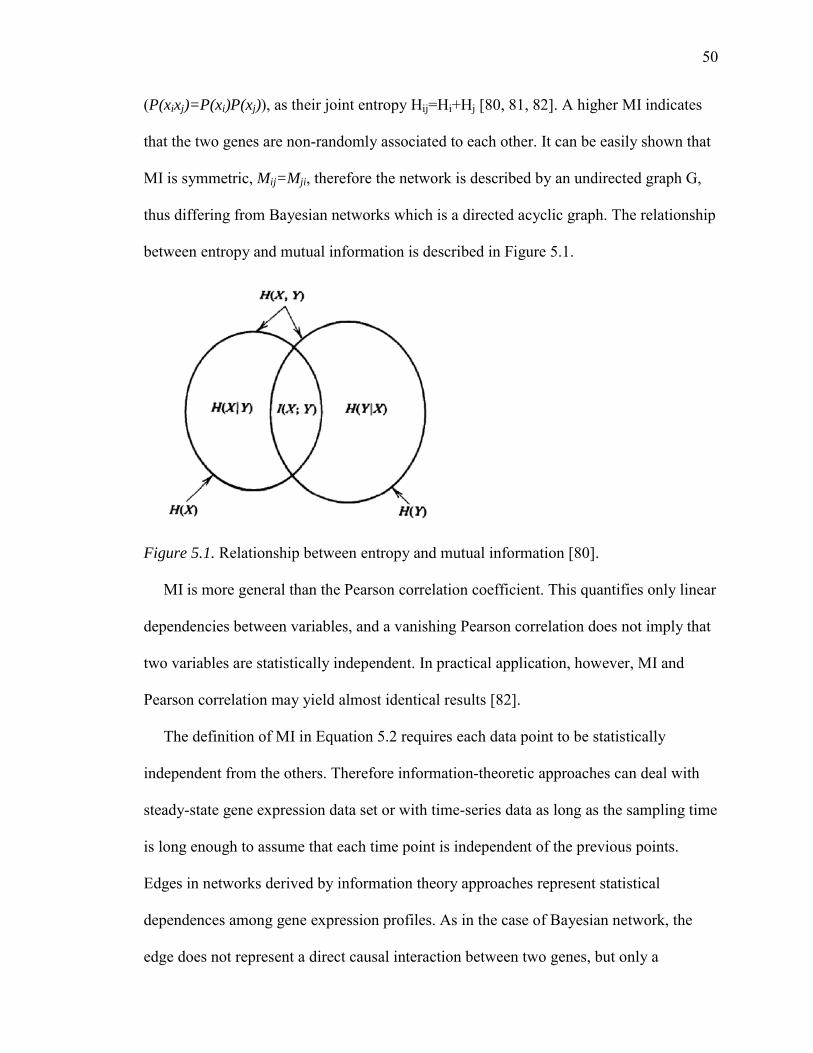
50
(P(xixj)=P(xi)P(xj)), as their joint entropy Hij=Hi+Hj [80, 81, 82]. A higher MI indicates
that the two genes are non-randomly associated to each other. It can be easily shown that
MI is symmetric, Mij=Mji, therefore the network is described by an undirected graph G,
thus differing from Bayesian networks which is a directed acyclic graph. The relationship
between entropy and mutual information is described in Figure 5.1.
Figure 5.1. Relationship between entropy and mutual information [80].
MI is more general than the Pearson correlation coefficient. This quantifies only linear
dependencies between variables, and a vanishing Pearson correlation does not imply that
two variables are statistically independent. In practical application, however, MI and
Pearson correlation may yield almost identical results [82].
The definition of MI in Equation 5.2 requires each data point to be statistically
independent from the others. Therefore information-theoretic approaches can deal with
steady-state gene expression data set or with time-series data as long as the sampling time
is long enough to assume that each time point is independent of the previous points.
Edges in networks derived by information theory approaches represent statistical
dependences among gene expression profiles. As in the case of Bayesian network, the
edge does not represent a direct causal interaction between two genes, but only a
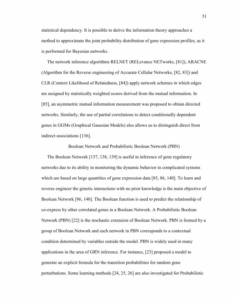
51
statistical dependency. It is possible to derive the information theory approaches a
method to approximate the joint probability distribution of gene expression profiles, as it
is performed for Bayesian networks.
The network inference algorithms RELNET (RELevance NETworks, [81]), ARACNE
(Algorithm for the Reverse engineering of Accurate Cellular Networks, [82, 83]) and
CLR (Context Likelihood of Relatedness, [84]) apply network schemes in which edges
are assigned by statistically weighted scores derived from the mutual information. In
[85], an asymmetric mutual information measurement was proposed to obtain directed
networks. Similarly, the use of partial correlations to detect conditionally dependent
genes in GGMs (Graphical Gaussian Models) also allows us to distinguish direct from
indirect associations [136].
Boolean Network and Probabilistic Boolean Network (PBN)
The Boolean Network [137, 138, 139] is useful in inference of gene regulatory
networks due to its ability in monitoring the dynamic behavior in complicated systems
which are based on large quantities of gene expression data [85, 86, 140]. To learn and
reverse engineer the genetic interactions with no prior knowledge is the main objective of
Boolean Network [86, 140]. The Boolean function is used to predict the relationship of
co-express by other correlated genes in a Boolean Network. A Probabilistic Boolean
Network (PBN) [22] is the stochastic extension of Boolean Network. PBN is formed by a
group of Boolean Network and each network in PBN corresponds to a contextual
condition determined by variables outside the model. PBN is widely used in many
applications in the area of GRN inference. For instance, [23] proposed a model to
generate an explicit formula for the transition probabilities for random gene
perturbations. Some learning methods [24, 25, 26] are also investigated for Probabilistic

52
Boolean Network. PBN and DBN are studied in terms of fundamental relationships [96]
considering the same joint probability distribution over common variables.
In a Boolean Network, by using the logical rules target gene’s expression level is
functionally related to other genes’ expression states. In addition, the target gene is
updated by other genes through a Boolean function. In a Boolean network, the gene
expression values need to be discretized into two states: namely on and off, which
corresponds to “activated” and “inhibited” respectively. A probabilistic Boolean network
consists of a family of Boolean networks and incorporates rule-based dependencies
between variables. In a PBN model, BNs are allowed to switch from one to another with
certain probabilities during state transitions.
Boolean Network
A Boolean network G(V,F) [87, 181] is defined by a set of variables representing
genes V={x1,x2,…,xn} (where xi {0,1} is a binary variable) and a set of Boolean functions
F={f1,f2,…,fn} which represents the transitional relationships between different time
points. A Boolean function ( ( ), ( ), … , ( )( )) with k(i) specified input nodes is
assigned to node xi. The gene status (state) at time point t+1 is determined by the values
of some other genes at previous time point t using one Boolean function fi taken from a
set of Boolean functions F . So we can define the transitions as in Equation 5.4:( + 1) = ( )( ), ( )( ), … , ( )( )( ) (5.4)where each xi is the expression value of gene i, if xi = 1, it is activated; if xi = 0, gene i is
inhibited. The variable ( ) is the mapping between gene networks at different time
points. Boolean function F is the rules of regulatory interactions between different genes.
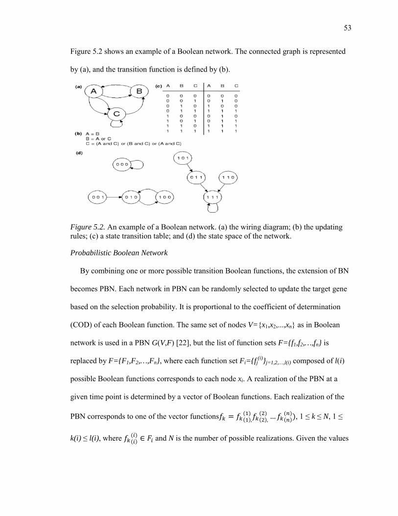
53
Figure 5.2 shows an example of a Boolean network. The connected graph is represented
by (a), and the transition function is defined by (b).
Figure 5.2. An example of a Boolean network. (a) the wiring diagram; (b) the updating rules; (c) a state transition table; and (d) the state space of the network.
Probabilistic Boolean Network
By combining one or more possible transition Boolean functions, the extension of BN
becomes PBN. Each network in PBN can be randomly selected to update the target gene
based on the selection probability. It is proportional to the coefficient of determination
(COD) of each Boolean function. The same set of nodes V={x1,x2,...,xn} as in Boolean
network is used in a PBN G(V,F) [22], but the list of function sets F={f1,f2,…,fn} is
replaced by F={F1,F2,…,Fn}, where each function set Fi={fj(i)}j=1,2,…,l(i) composed of l(i)
possible Boolean functions corresponds to each node xi. A realization of the PBN at a
given time point is determined by a vector of Boolean functions. Each realization of the
PBN corresponds to one of the vector functions = ( ),( ) ( ),( ) … ( )( )), 1 k N, 1
k(i) l(i), where ( )( ) and N is the number of possible realizations. Given the values
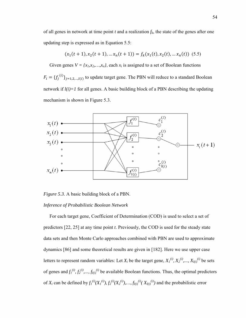
54
of all genes in network at time point t and a realization fk, the state of the genes after one
updating step is expressed as in Equation 5.5:( ( + 1), ( + 1), … ( + 1)) = ( ( ), ( ), … ( )) (5.5)
Given genes V = {x1,x2,…,xn}, each xi is assigned to a set of Boolean functions= { ( )} , ,…, ( ) to update target gene. The PBN will reduce to a standard Boolean
network if l(i)=1 for all genes. A basic building block of a PBN describing the updating
mechanism is shown in Figure 5.3.
Figure 5.3. A basic building block of a PBN.
Inference of Probabilistic Boolean Network
For each target gene, Coefficient of Determination (COD) is used to select a set of
predictors [22, 25] at any time point t. Previously, the COD is used for the steady state
data sets and then Monte Carlo approaches combined with PBN are used to approximate
dynamics [86] and some theoretical results are given in [182]. Here we use upper case
letters to represent random variables: Let Xi be the target gene, X1(i), X2
(i),..., Xl(i)(i) be sets
of genes and f1(i), f2
(i),..., fl(i)(i) be available Boolean functions. Thus, the optimal predictors
of Xi can be defined by f1(i)(X1
(i)), f2(i)(X2
(i)),…, fl(i)(i)( Xl(i)
(i)) and the probabilistic error
55
measure i, fk(i)(Xk
(i))). For each k, the COD for Xi relative to the
conditioning set Xk(i) is defined by Equation 5.6:
= ( , ( )( ( ))) (5.6)
where is the error of the best estimate of [25].
Based on the above equations [22, 25], the Boolean functions which are corresponding
to the highest CODs will be chosen in the probabilistic network. The selected Boolean
functions will be used to predict the state of gene (gene expression status) on the
subsequent time point as well as to infer gene regulatory networks.
Bayesian Network and Dynamic Bayesian Network (DBN)
Due to the probabilistic nature of Bayesian network, it is widely used in reconstruction
of gene regulatory network from time series dataset. Dynamic Bayesian network is the
temporal extension of Bayesian network. DBN can be used to model complex temporal
stochastic processes as it captures several other often used modeling frameworks such as
hidden Markov models (and its variants) and Kalman filter models. The drawbacks of
Bayesian network approach makes it fail to capture temporal information and unable to
model cyclic networks. The Dynamic Bayesian network approaches solved such
problems as it is better suited for characterizing time series gene expression dataset. A lot
of researches have been conducted to infer GRNs from gene expression data using BN
and DBN. For example, the stochastic machine learning algorithm is used to model
genetic interactions are capable of handling dataset with missing variables [29]. In
addition, Min Zou et al. [28] proposed a new DBN-based approach, in which the number
of potential regulators is limited in order to reduce search space. Yu, J. et al. [27]
developed a simulation approach to take advantage of DBN algorithm, especially in the

56
case of limited biological dataset. In [30], a higher order Markov DBN approach is
proposed in order to model multiple time units in a delayed GRN. Also, likelihood
maximization algorithms have been used to predict hidden parameters and impute
missing gene expression values [31].
Bayesian Network
A Bayesian network is a graphical model for probabilistic relationships among a set of
random variables Xi, where i=1…n. Such relationships are represented in a structure of
directed acyclic graph G, in which the vertices are random variables Xi. The relationship
between the variables are indicated as a joint probability distribution P(X1, …, Xn) which
is consistent with the independence assertions embedded in the graph G and has the form
as in Equation 5.7:
( , … , ) = ( = | = , … , = (5.7)where the p+1 genes, on which the probability is conditioned, are called the parents of
gene i and represent its regulators, and the joint probability density is expressed as a
product of conditional probabilities by applying the chain rule of probabilities and
independence. This rule is based on the Bayes’ theorem:
P(A,B)=P(B||A)*P(A)=P(A||B)*P(B). The joint probability distribution can be
decomposed as the product of conditional probabilities [26, 94]. A simple example of
Bayesian network is shown in Figure 5.4.
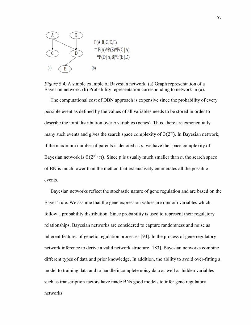
57
Figure 5.4. A simple example of Bayesian network. (a) Graph representation of a Bayesian network. (b) Probability representation corresponding to network in (a).
The computational cost of DBN approach is expensive since the probability of every
possible event as defined by the values of all variables needs to be stored in order to
describe the joint distribution over n variables (genes). Thus, there are exponentially
many such events and gives the search space complexity of (2 ). In Bayesian network,
if the maximum number of parents is denoted as p, we have the space complexity of
Bayesian network is (2 ). Since p is usually much smaller than n, the search space
of BN is much lower than the method that exhaustively enumerates all the possible
events.
Bayesian networks reflect the stochastic nature of gene regulation and are based on the
Bayes’ rule. We assume that the gene expression values are random variables which
follow a probability distribution. Since probability is used to represent their regulatory
relationships, Bayesian networks are considered to capture randomness and noise as
inherent features of genetic regulation processes [94]. In the process of gene regulatory
network inference to derive a valid network structure [183], Bayesian networks combine
different types of data and prior knowledge. In addition, the ability to avoid over-fitting a
model to training data and to handle incomplete noisy data as well as hidden variables
such as transcription factors have made BNs good models to infer gene regulatory
networks.

58
Three essential elements in the process of learning a BN: model selection, parameter
learning as well as model scoring [184]. In model selection, instead of using brute-force
search algorithm, heuristics methods are usually used to learn a BN efficiently since the
brute-force search will grow exponentially as the number of genes increase in a directed
acyclic graph. In parameter learning, the goal is to find the best conditional probabilities
(CP) for each node in a graph and experimental dataset. In model scoring, each candidate
model will be scored and higher score indicates the network model (the DAG and the
learned CP distribution) better fits to the data. The inferred GRN will be the model with
the highest score.
Dynamic Bayesian Network
The drawbacks of Bayesian network approach makes it fail to capture temporal
information and unable to model cyclic networks. The Dynamic Bayesian network
(DBN) [185] approaches solved such problems as it is better suited for characterizing
time series gene expression dataset. DBN can be used to model complex temporal and
cyclic relationships of genes by incorporating time course (or time slice) information.
Here we are modeling a dynamic system while the gene regulatory network does not
change over time. By incorporating time series information, DBN represents the cyclic
relations among genes in Figure 5.5.
Figure 5.5. Static Bayesian network and DBN.
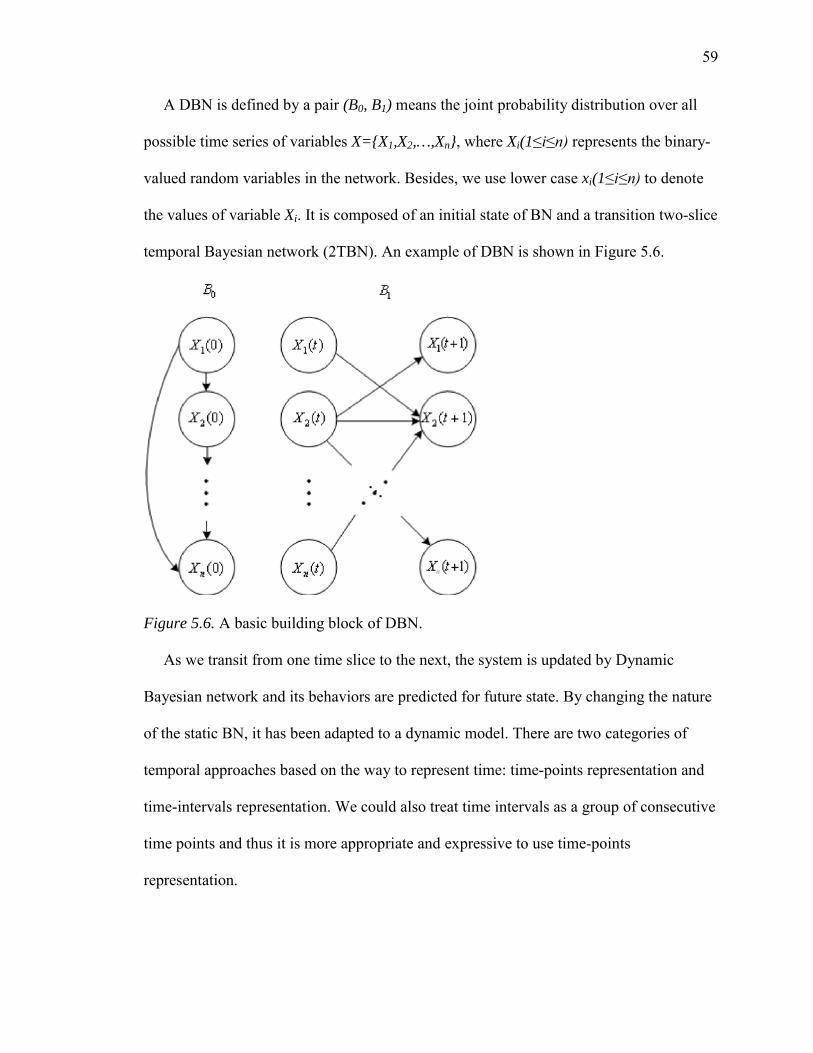
59
A DBN is defined by a pair (B0, B1) means the joint probability distribution over all
possible time series of variables X={X1,X2,…,Xn}, where Xi(1 represents the binary-
valued random variables in the network. Besides, we use lower case xi(1 to denote
the values of variable Xi. It is composed of an initial state of BN and a transition two-slice
temporal Bayesian network (2TBN). An example of DBN is shown in Figure 5.6.
Figure 5.6. A basic building block of DBN.
As we transit from one time slice to the next, the system is updated by Dynamic
Bayesian network and its behaviors are predicted for future state. By changing the nature
of the static BN, it has been adapted to a dynamic model. There are two categories of
temporal approaches based on the way to represent time: time-points representation and
time-intervals representation. We could also treat time intervals as a group of consecutive
time points and thus it is more appropriate and expressive to use time-points
representation.

60
Leaning Bayesian Network
In general, it is difficult or hardly to manually capture the complete structure and
parameters of Bayesian network. Therefore, the task of learning BN from gene
expression data becomes very important. Estimating the parameters of the model and
inferring the structure of the GRN are two key elements to learn a Bayesian network from
a given gene expression data.
Parameter Learning
For a given graph G, maximizing the joint likelihood of gene expression data is
generally used to estimate the parameters (also known as generative parameter learning
[186]). Recently, the algorithms of maximizing conditional likelihood of the class
variables given the observed evidence variables have been proposed in order to learn the
parameters since BNs are widely used as classifiers. Such algorithms are called
discriminative parameter learning [187, 188, 189].
Generative Parameter Learning
Given a set of training data , which is composed of a set of independent and
identically distributed instances [x1,…,xN], where all components are observed,
generative parameter learning methods estimate the parameters of a BN either by directly
maximizing the joint likelihood of training data, or by computing the posterior over
parameters given a prior distribution
The method of maximum likelihood estimation uses the conditional independence
assumptions encoded in the structure. The joint log likelihood of training data can be
factored in Equation 5.8:log ( | ) = log ( | ( ), ) (5.8)
61
The second generative method is called maximum a posteriori estimation (MAP).
Bayesian networks allow us to incorporate prior domain knowledge and use it to
effectively avoid the problem of over-fitting, especially when limited number of training
datasets is given. Given a prior density , we can learn the parameters to maximize the
posterior as in Equation 5.9:
log ( | ) = log ( ) ( | )( ) (5.9)This is equivalent to maximizing because P(D) is invariant with respect to .
A commonly used algorithm to learn BN from incomplete data is the Expectation
Maximization (EM) method.
Discriminative Parameter Learning
Due to the shortcoming of inconsistency with its performance when optimizing a
criterion such as maximum likelihood or MAP, the generative parameter learning method
is not the best way to train classification models. Recently, an improved discriminative
approach for supervised parameter learning that takes conditional likelihood as the
optimization criterion is proposed in [187, 188, 189, 190].
Although it is easy to learn parameters given complete dataset, to find the global
maximum is still difficult when using the discriminative conditional likelihood criterion
for general Bayesian networks. To find the parameters for a fixed BN structure that
maximize the conditional likelihood of a given sample of incomplete data is a NP-hard
problem as in [187].
Structural Learning
If the topology of the target Bayesian network is fixed, the task is to estimate the CPTs
or CPDs for every node in the network. Or else, if the topology is unknown, structure

62
learning is required to learn the graph topology of the target BN before the parameters
could be determined. In addition, the dataset could be either complete or incomplete for
BN learning. Thus, four cases of learning structure of BNs are summarized based on the
above varieties [191]. Table 5.1 shows the four cases for learning Bayesian network
structure.
Table 5.1
Methods for Learning Bayesian Network Structure and Parameter Determination
Structure/Observability Method
Known, full Sample statistics
Known, partial EM or gradient ascent
Unknown, full Search through model space
Unknown, partial Structural EM
Full observability means that the values of all variables are known; partial
observability means that we do not know the values of some of the variables. This might
be because they cannot be measured (in which case they are usually called hidden
variables), or because they just happen to be unmeasured in the training data (in which
case they are called missing variables). Unknown structure means we do not know the
complete topology of the gene regulatory network. Usually we know some parts of it, or
at least know some properties of the graph, for instance, the maximum number of parents
(fan-in) that a node can take in, and we may know that nodes of a certain “type” only
connect to other nodes of the same type. Such constraints are called prior knowledge.
Therefore, the learning task becomes parameter estimation when we know the structure
of the model.
DBN Implementation
63
Kevin Murphy [185, 191] implemented a Dynamic Bayesian Network toolbox using
the mathematical programming language (MATLAB), namely Bayes Net toolbox (BNT).
It is an open-source package for directed graphical models and supports many types of
nodes (probability distributions), exact and approximate inference, parameter and
structure learning, and static as well as dynamic models. BNT can be freely downloaded
from [192]. In Murphy’s method, the gene expression data was first discretized from
continuous form and the number of discrete steps is kept as low as possible. In general,
three discrete steps were used: one for unchanged, one for up-regulated and one for
down-regulated expression values. Then the BNT function learn_struct_dbn_reveal is
called to conduct structural learning, which employs the REVEAL algorithm [193]. The
BNT function called draw_layout is used to visualize the generated inter-slice adjacency
matrix that represents the transition network. A number of other implementations of DBN
method using time series gene expression data are proposed in [27, 28, 29, 30].
Time-Delayed Dynamic Bayesian Network
There are two major problems with Murphy’s DBN method which greatly reduce their
effectiveness. The first is the lack of a systematic way to determine the time lag of
biological relevance. Such problem results in a relatively low accuracy of inferring gene
regulatory networks. The second is the excessive computational cost of huge searching
space. Only limited number of genes can be modeled and reconstructing GRN. Thus, Min
Zou et al. [28] introduces a DBN-based analysis that can predict gene regulatory
networks from time course expression data with significantly increased accuracy and
reduced computational time. Based on the characteristics of our microarray dataset, Zou’s
implementation is used to reconstruct gene regulatory network. Figure 5.7 shows the
process of approach in [28]: (1) Identification of the initial expression changes; (2)
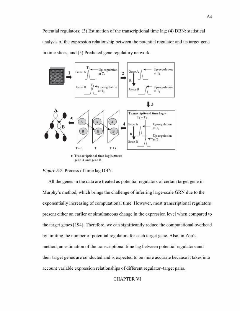
64
Potential regulators; (3) Estimation of the transcriptional time lag; (4) DBN: statistical
analysis of the expression relationship between the potential regulator and its target gene
in time slices; and (5) Predicted gene regulatory network.
Figure 5.7. Process of time lag DBN.
All the genes in the data are treated as potential regulators of certain target gene in
Murphy’s method, which brings the challenge of inferring large-scale GRN due to the
exponentially increasing of computational time. However, most transcriptional regulators
present either an earlier or simultaneous change in the expression level when compared to
the target genes [194]. Therefore, we can significantly reduce the computational overhead
by limiting the number of potential regulators for each target gene. Also, in Zou’s
method, an estimation of the transcriptional time lag between potential regulators and
their target genes are conducted and is expected to be more accurate because it takes into
account variable expression relationships of different regulator–target pairs.
CHAPTER VI
65
MICROARRAY DATA MINING: CASE STUDY
Military-related activities produce many different chemicals, a portion of which
inevitably contaminate soil. Neurotoxicity has been associated with energetic
compounds, TNT and RDX as well as their degradation products. Monitoring, assessing
and predicting the risks these chemicals pose when released require fundamental
knowledge on how neurotoxicity occurs. A major barrier to development of predictive
risk tools is the lack of an appropriate and detailed model of the molecular events leading
to neurotoxicity when organisms are exposed to contaminated soils. We are interested to
identify and discover how components involved in neurotransmission within the soil
organism Eisenia fetida interact and are affected by neurotoxicants. Understanding this
network of interactions is essential for development of predictive risk models in the
future.
As a terrestrial toxicological model organism, E. fetida has a simple but efficient
nervous system that is an excellent model to study the major neurotransmitters and
synaptic pathways. Many neurotransmission pathways are conserved between E. fetida
and vertebrates. Previously, we discovered that at sub-lethal doses, TNT affected genes
involved in neurological processes. At appropriate dosages RDX both exhibit reversible
neurotoxicity in E. fetida. However, it is unclear whether RDX has affected other
neurotransmission pathways and how genes involved in these pathways interact in a
broader network context to compensate for or to cope with the perturbation caused by
exposure to a neurotoxicant. Therefore, a system biology approach is used to discover
effects of neurotoxicants on neurotransmitter pathways related gene expression in a gene
regulatory network (GRN). First, the data set of gene expression values are preprocessed
and analyzed by ISML pipeline to discover classifier genes that significantly affected by
66
the chemical and identify relevant pathways/GRNs for further study. Then, reference
networks of user-selected pathways in the organism of interest were built by RefNet
toolbox. Last, a set of genes in a certain pathway were selected and used to reconstruct
gene regulatory networks in order to discover the mechanisms of perturbations of the
network after being exposed to the chemical. Two case studies will be described in the
following section to walk through the procedure.
Multi-Class Earthworm Microarray Dataset
DNA microarray, a maturing genomic technology, has been used extensively as a
diagnostic tool to complement traditional approaches such as histopathological
examination for various diseases (particularly cancers) because microscopic appearances
sometimes can be deceiving [141, 142, 143, 144]. Microarrays have also successfully
served as a research tool in discovering novel drug targets [145] and disease- or toxicity-
related biomarker genes for cancer classification [146]. In ecological risk assessment,
indigenous species such as fish and earthworms are often used as bioindicators for
adverse effects caused by environmental contaminants. Previously, we developed an
earthworm (Eisenia fetida) cDNA microarray to analyze toxicological mechanisms for
two military-unique explosive compounds 2,4,6-trinitrotolune (TNT) and 1,3,5-trinitro-
1,3,5-triazacyclohexane (also known as Royal Demolition eXplosive or RDX) [147, 148].
These two compounds exhibit distinctive toxicological properties that are accompanied
by significantly different gene expression profiles in the earthworm E. fetida [147, 148,
149], which has motivated us to look further into toxicant- or toxicity-specific signature
genes/biomarkers. The second motivation comes from the fact that many diagnostic
assays exist for human diseases while very few are available for evaluating impacts on
environmentally-relevant organisms. Gross survival, growth and reproduction rates are

67
often used as assessment endpoints without reflecting the diseased population of affected
animals that is an important part of long-term impact assessment. The last motivation is
that computational tools such as machine learning techniques have been widely used in
cancer and toxicant classification with microarray data but rarely applied in microarray
data analysis of environmentally relevant organisms [150, 151, 152].
From a regulatory standpoint, there is an increasing and continuous demand for more
rapid, more accurate and more predictive assays due to the already large, but still
growing, number of man-made chemicals released into the environment [153]. Molecular
endpoints such as gene expression that may reflect phenotypic disease symptoms
manifested later at higher biological levels (e.g., cell, tissue, organ, or organism) are
potentially biomarkers that meet such demands. As a high throughput tool, microarrays
simultaneously measure thousands of biologically-relevant endpoints (gene expression).
However, to apply this tool to animals under field conditions, one critical hurdle to
overcome is the separation of toxicity-induced signals from background noise associated
with environmental variation and other confounding factors such as animal age, genetic
make-up, physiological state and exposure length and route [150,151]. A common
approach to biomarker discovery is to screen genome- or transcriptome-wide gene
expression responses and identify a small subset of genes capable of discriminating
animals that received different treatments, or predicting the class of unknown samples. It
is relatively less challenging to identify differentially expressed genes from two or more
classes of samples. However, the search for an optimal and small subset of genes that has
a high discriminatory power in classifying field samples often having multiple classes is
much more complicated.
68
For instance, Falciani and colleagues profiled gene expression of 77 hepatic samples
of European flounder (Platichthys flesus) collected from six different environmental sites
[150]. Using a multivariate variable selection coupled with a statistical modelling
procedure they demonstrated that the accuracy of predicting the geographical site of
origin based on gene expression signatures in flounder livers was limited to specific sites.
After incorporating prior knowledge and data from laboratory exposures to individual
toxicants, they were able to limit the search space for a combination of effective classifier
genes and built a very accurate model consisting of only 17 genes for classification of all
the different environmental sites. Similarly, Nota and co-workers recently identified a set
of 188 genes from expression profiles of the springtail (Folsomia candida) exposed to a
soil spiked with six different metals using the uncorrelated shrunken centroid method,
and predicted an independent test soils set with an accuracy of 83% but failed on field
soils collected from two cobalt-contaminated sites using this gene set [151]. Several other
studies also reported a varying degree of success in the identification of classifier genes
in both aquatic species like the zebrafish (Danio rerio) [152], the common carp Cyprinus
carpio [154] and the water flea Daphnia magna [155], and terrestrial organisms such as
the earthworm Lumbricus rubellus [156].
As part of a larger effort towards discovering novel biomarkers for ecological risk
assessment of military lands, researchers at the Environmental Laboratory of U.S. Army
Engineer Research and Development Center have developed a 15208-oligonucleotide E.
fetida array, and generated a large-scale microarray dataset from a laboratory study where
earthworms (E. fetida) were exposed to various concentrations of TNT or RDX for
various lengths of time in soil, mimicking field exposure scenarios (see below for
details). The objective of the current study was to identify a small set of classifier genes
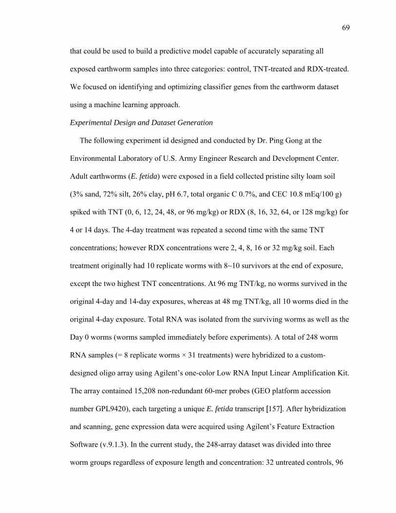
69
that could be used to build a predictive model capable of accurately separating all
exposed earthworm samples into three categories: control, TNT-treated and RDX-treated.
We focused on identifying and optimizing classifier genes from the earthworm dataset
using a machine learning approach.
Experimental Design and Dataset Generation
The following experiment id designed and conducted by Dr. Ping Gong at the
Environmental Laboratory of U.S. Army Engineer Research and Development Center.
Adult earthworms (E. fetida) were exposed in a field collected pristine silty loam soil
(3% sand, 72% silt, 26% clay, pH 6.7, total organic C 0.7%, and CEC 10.8 mEq/100 g)
spiked with TNT (0, 6, 12, 24, 48, or 96 mg/kg) or RDX (8, 16, 32, 64, or 128 mg/kg) for
4 or 14 days. The 4-day treatment was repeated a second time with the same TNT
concentrations; however RDX concentrations were 2, 4, 8, 16 or 32 mg/kg soil. Each
treatment originally had 10 replicate worms with 8~10 survivors at the end of exposure,
except the two highest TNT concentrations. At 96 mg TNT/kg, no worms survived in the
original 4-day and 14-day exposures, whereas at 48 mg TNT/kg, all 10 worms died in the
original 4-day exposure. Total RNA was isolated from the surviving worms as well as the
Day 0 worms (worms sampled immediately before experiments). A total of 248 worm
RNA samples (= 8 replicate worms × 31 treatments) were hybridized to a custom-
designed oligo array using Agilent’s one-color Low RNA Input Linear Amplification Kit.
The array contained 15,208 non-redundant 60-mer probes (GEO platform accession
number GPL9420), each targeting a unique E. fetida transcript [157]. After hybridization
and scanning, gene expression data were acquired using Agilent’s Feature Extraction
Software (v.9.1.3). In the current study, the 248-array dataset was divided into three
worm groups regardless of exposure length and concentration: 32 untreated controls, 96
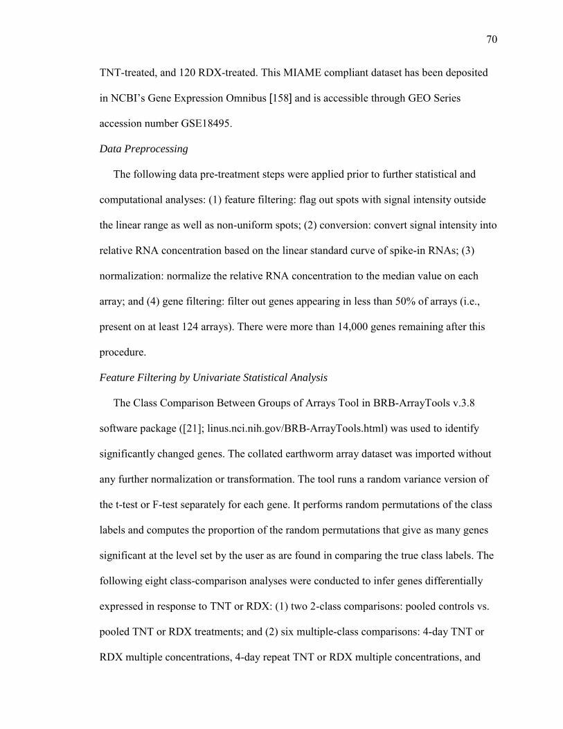
70
TNT-treated, and 120 RDX-treated. This MIAME compliant dataset has been deposited
in NCBI’s Gene Expression Omnibus [158] and is accessible through GEO Series
accession number GSE18495.
Data Preprocessing
The following data pre-treatment steps were applied prior to further statistical and
computational analyses: (1) feature filtering: flag out spots with signal intensity outside
the linear range as well as non-uniform spots; (2) conversion: convert signal intensity into
relative RNA concentration based on the linear standard curve of spike-in RNAs; (3)
normalization: normalize the relative RNA concentration to the median value on each
array; and (4) gene filtering: filter out genes appearing in less than 50% of arrays (i.e.,
present on at least 124 arrays). There were more than 14,000 genes remaining after this
procedure.
Feature Filtering by Univariate Statistical Analysis
The Class Comparison Between Groups of Arrays Tool in BRB-ArrayTools v.3.8
software package ([21]; linus.nci.nih.gov/BRB-ArrayTools.html) was used to identify
significantly changed genes. The collated earthworm array dataset was imported without
any further normalization or transformation. The tool runs a random variance version of
the t-test or F-test separately for each gene. It performs random permutations of the class
labels and computes the proportion of the random permutations that give as many genes
significant at the level set by the user as are found in comparing the true class labels. The
following eight class-comparison analyses were conducted to infer genes differentially
expressed in response to TNT or RDX: (1) two 2-class comparisons: pooled controls vs.
pooled TNT or RDX treatments; and (2) six multiple-class comparisons: 4-day TNT or
RDX multiple concentrations, 4-day repeat TNT or RDX multiple concentrations, and
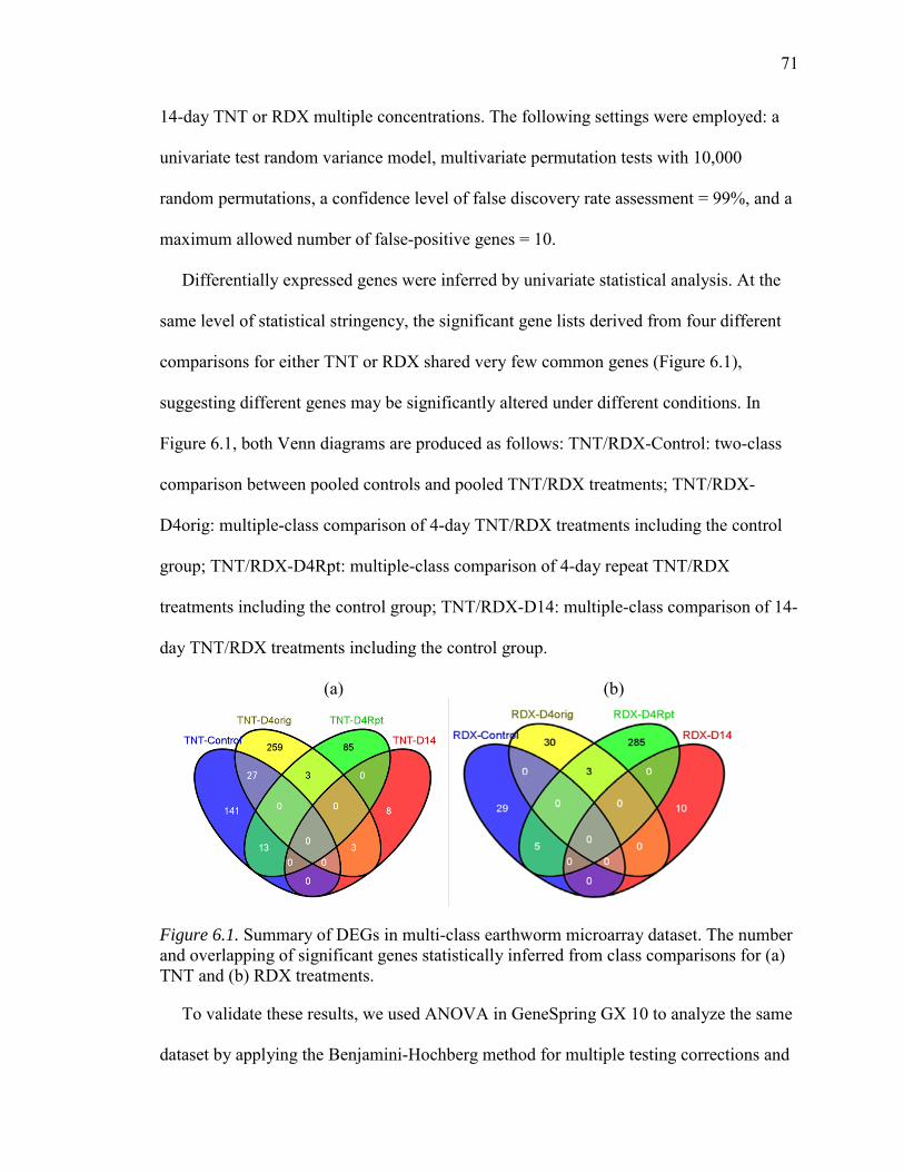
71
14-day TNT or RDX multiple concentrations. The following settings were employed: a
univariate test random variance model, multivariate permutation tests with 10,000
random permutations, a confidence level of false discovery rate assessment = 99%, and a
maximum allowed number of false-positive genes = 10.
Differentially expressed genes were inferred by univariate statistical analysis. At the
same level of statistical stringency, the significant gene lists derived from four different
comparisons for either TNT or RDX shared very few common genes (Figure 6.1),
suggesting different genes may be significantly altered under different conditions. In
Figure 6.1, both Venn diagrams are produced as follows: TNT/RDX-Control: two-class
comparison between pooled controls and pooled TNT/RDX treatments; TNT/RDX-
D4orig: multiple-class comparison of 4-day TNT/RDX treatments including the control
group; TNT/RDX-D4Rpt: multiple-class comparison of 4-day repeat TNT/RDX
treatments including the control group; TNT/RDX-D14: multiple-class comparison of 14-
day TNT/RDX treatments including the control group.
(a) (b)
Figure 6.1. Summary of DEGs in multi-class earthworm microarray dataset. The number and overlapping of significant genes statistically inferred from class comparisons for (a) TNT and (b) RDX treatments.
To validate these results, we used ANOVA in GeneSpring GX 10 to analyze the same
dataset by applying the Benjamini-Hochberg method for multiple testing corrections and
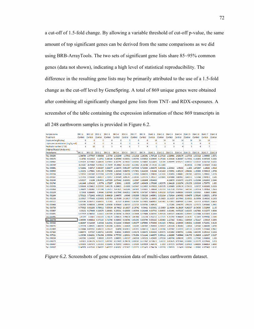
72
a cut-off of 1.5-fold change. By allowing a variable threshold of cut-off p-value, the same
amount of top significant genes can be derived from the same comparisons as we did
using BRB-ArrayTools. The two sets of significant gene lists share 85~95% common
genes (data not shown), indicating a high level of statistical reproducibility. The
difference in the resulting gene lists may be primarily attributed to the use of a 1.5-fold
change as the cut-off level by GeneSpring. A total of 869 unique genes were obtained
after combining all significantly changed gene lists from TNT- and RDX-exposures. A
screenshot of the table containing the expression information of these 869 transcripts in
all 248 earthworm samples is provided in Figure 6.2.
Figure 6.2. Screenshots of gene expression data of multi-class earthworm dataset.
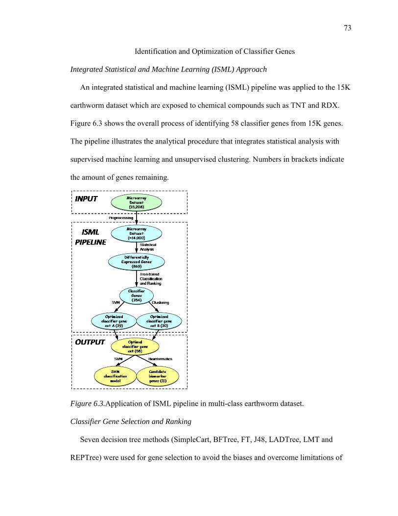
73
Identification and Optimization of Classifier Genes
Integrated Statistical and Machine Learning (ISML) Approach
An integrated statistical and machine learning (ISML) pipeline was applied to the 15K
earthworm dataset which are exposed to chemical compounds such as TNT and RDX.
Figure 6.3 shows the overall process of identifying 58 classifier genes from 15K genes.
The pipeline illustrates the analytical procedure that integrates statistical analysis with
supervised machine learning and unsupervised clustering. Numbers in brackets indicate
the amount of genes remaining.
Figure 6.3.Application of ISML pipeline in multi-class earthworm dataset.
Classifier Gene Selection and Ranking
Seven decision tree methods (SimpleCart, BFTree, FT, J48, LADTree, LMT and
REPTree) were used for gene selection to avoid the biases and overcome limitations of
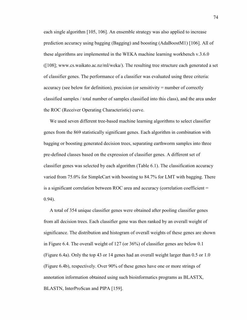
74
each single algorithm [105, 106]. An ensemble strategy was also applied to increase
prediction accuracy using bagging (Bagging) and boosting (AdaBoostM1) [106]. All of
these algorithms are implemented in the WEKA machine learning workbench v.3.6.0
([108]; www.cs.waikato.ac.nz/ml/weka/). The resulting tree structure each generated a set
of classifier genes. The performance of a classifier was evaluated using three criteria:
accuracy (see below for definition), precision (or sensitivity = number of correctly
classified samples / total number of samples classified into this class), and the area under
the ROC (Receiver Operating Characteristic) curve.
We used seven different tree-based machine learning algorithms to select classifier
genes from the 869 statistically significant genes. Each algorithm in combination with
bagging or boosting generated decision trees, separating earthworm samples into three
pre-defined classes based on the expression of classifier genes. A different set of
classifier genes was selected by each algorithm (Table 6.1). The classification accuracy
varied from 75.0% for SimpleCart with boosting to 84.7% for LMT with bagging. There
is a significant correlation between ROC area and accuracy (correlation coefficient =
0.94).
A total of 354 unique classifier genes were obtained after pooling classifier genes
from all decision trees. Each classifier gene was then ranked by an overall weight of
significance. The distribution and histogram of overall weights of these genes are shown
in Figure 6.4. The overall weight of 127 (or 36%) of classifier genes are below 0.1
(Figure 6.4a). Only the top 43 or 14 genes had an overall weight larger than 0.5 or 1.0
(Figure 6.4b), respectively. Over 90% of these genes have one or more strings of
annotation information obtained using such bioinformatics programs as BLASTX,
BLASTN, InterProScan and PIPA [159].
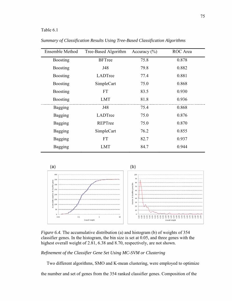
75
Table 6.1
Summary of Classification Results Using Tree-Based Classification Algorithms
Ensemble Method Tree-Based Algorithm Accuracy (%) ROC Area
Boosting BFTree 75.8 0.878
Boosting J48 79.8 0.882
Boosting LADTree 77.4 0.881
Boosting SimpleCart 75.0 0.868
Boosting FT 83.5 0.930
Boosting LMT 81.8 0.936
Bagging J48 75.4 0.868
Bagging LADTree 75.0 0.876
Bagging REPTree 75.0 0.870
Bagging SimpleCart 76.2 0.855
Bagging FT 82.7 0.937
Bagging LMT 84.7 0.944
Figure 6.4. The accumulative distribution (a) and histogram (b) of weights of 354classifier genes. In the histogram, the bin size is set at 0.05, and three genes with the highest overall weight of 2.81, 6.38 and 8.70, respectively, are not shown.
Refinement of the Classifier Gene Set Using MC-SVM or Clustering
Two different algorithms, SMO and K-mean clustering, were employed to optimize
the number and set of genes from the 354 ranked classifier genes. Composition of the
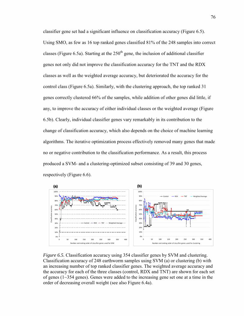
76
classifier gene set had a significant influence on classification accuracy (Figure 6.5).
Using SMO, as few as 16 top ranked genes classified 81% of the 248 samples into correct
classes (Figure 6.5a). Starting at the 250th gene, the inclusion of additional classifier
genes not only did not improve the classification accuracy for the TNT and the RDX
classes as well as the weighted average accuracy, but deteriorated the accuracy for the
control class (Figure 6.5a). Similarly, with the clustering approach, the top ranked 31
genes correctly clustered 66% of the samples, while addition of other genes did little, if
any, to improve the accuracy of either individual classes or the weighted average (Figure
6.5b). Clearly, individual classifier genes vary remarkably in its contribution to the
change of classification accuracy, which also depends on the choice of machine learning
algorithms. The iterative optimization process effectively removed many genes that made
no or negative contribution to the classification performance. As a result, this process
produced a SVM- and a clustering-optimized subset consisting of 39 and 30 genes,
respectively (Figure 6.6).
Figure 6.5. Classification accuracy using 354 classifier genes by SVM and clustering. Classification accuracy of 248 earthworm samples using SVM (a) or clustering (b) with an increasing number of top ranked classifier genes. The weighted average accuracy and the accuracy for each of the three classes (control, RDX and TNT) are shown for each set of genes (1~354 genes). Genes were added to the increasing gene set one at a time in the order of decreasing overall weight (see also Figure 6.4a).
0%
10%
20%
30%
40%
50%
60%
70%
80%
90%
100%
0 50 100 150 200 250 300 350 400
Number and ranking order of classifier genes used for clustering
Clas
sific
atio
n ac
cura
cy
Control RDX TNT Weighted Average
0%
10%
20%
30%
40%
50%
60%
70%
80%
90%
100%
0 50 100 150 200 250 300 350 400
Number and ranking order of classifier genes used for SVM
Clas
sific
atio
n ac
cura
cy
Control RDX TNT Weighted Average
(a) (b)
0%
10%
20%
30%
40%
50%
60%
70%
80%
90%
100%
0 50 100 150 200 250 300 350 400
Number and ranking order of classifier genes used for clustering
Clas
sific
atio
n ac
cura
cy
Control RDX TNT Weighted Average
0%
10%
20%
30%
40%
50%
60%
70%
80%
90%
100%
0 50 100 150 200 250 300 350 400
Number and ranking order of classifier genes used for SVM
Clas
sific
atio
n ac
cura
cy
Control RDX TNT Weighted Average
(a) (b)
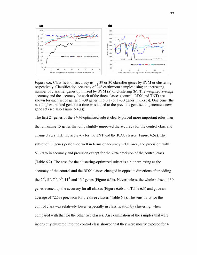
77
Figure 6.6. Classification accuracy using 39 or 30 classifier genes by SVM or clustering, respectively. Classification accuracy of 248 earthworm samples using an increasing number of classifier genes optimized by SVM (a) or clustering (b). The weighted average accuracy and the accuracy for each of the three classes (control, RDX and TNT) are shown for each set of genes (1~39 genes in 6.6(a) or 1~30 genes in 6.6(b)). One gene (the next highest ranked gene) at a time was added to the previous gene set to generate a new gene set (see also Figure 6.4(a)).
The first 24 genes of the SVM-optimized subset clearly played more important roles than
the remaining 15 genes that only slightly improved the accuracy for the control class and
changed very little the accuracy for the TNT and the RDX classes (Figure 6.5a). The
subset of 39 genes performed well in terms of accuracy, ROC area, and precision, with
83~91% in accuracy and precision except for the 76% precision of the control class
(Table 6.2). The case for the clustering-optimized subset is a bit perplexing as the
accuracy of the control and the RDX classes changed in opposite directions after adding
the 2nd, 5th, 7th, 9th, 11th and 13th genes (Figure 6.5b). Nevertheless, the whole subset of 30
genes evened up the accuracy for all classes (Figure 6.6b and Table 6.3) and gave an
average of 72.5% precision for the three classes (Table 6.3). The sensitivity for the
control class was relatively lower, especially in classification by clustering, when
compared with that for the other two classes. An examination of the samples that were
incorrectly clustered into the control class showed that they were mostly exposed for 4
(a) (b)
0%
10%
20%
30%
40%
50%
60%
70%
80%
90%
100%
0 5 10 15 20 25 30 35 40
Number and ranking of classifier genes in the SVM-optimized gene set
Clas
sific
atio
n ac
cura
cy o
f cla
ssifi
er g
ene
set
Control RDX TNT Weighted average
0%
10%
20%
30%
40%
50%
60%
70%
80%
90%
100%
0 5 10 15 20 25 30
Number and ranking of classifier genes in the clustering-optimized gene set
Clas
sific
atio
n ac
cura
cy
Control RDX TNT Weighted Average
(a) (b)
0%
10%
20%
30%
40%
50%
60%
70%
80%
90%
100%
0 5 10 15 20 25 30 35 40
Number and ranking of classifier genes in the SVM-optimized gene set
Clas
sific
atio
n ac
cura
cy o
f cla
ssifi
er g
ene
set
Control RDX TNT Weighted average
0%
10%
20%
30%
40%
50%
60%
70%
80%
90%
100%
0 5 10 15 20 25 30
Number and ranking of classifier genes in the clustering-optimized gene set
Clas
sific
atio
n ac
cura
cy
Control RDX TNT Weighted Average
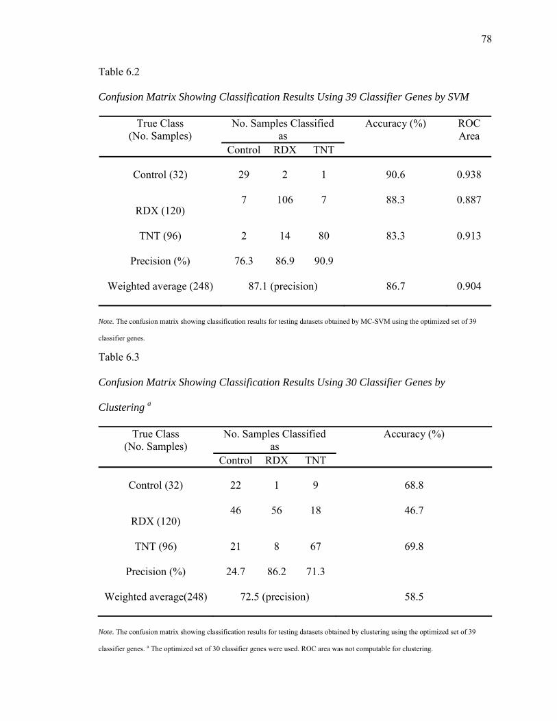
78
Table 6.2
Confusion Matrix Showing Classification Results Using 39 Classifier Genes by SVM
True Class(No. Samples)
No. Samples Classified as
Accuracy (%) ROC Area
Control RDX TNT
Control (32) 29 2 1 90.6 0.938
RDX (120)7 106 7 88.3 0.887
TNT (96) 2 14 80 83.3 0.913
Precision (%) 76.3 86.9 90.9
Weighted average (248) 87.1 (precision) 86.7 0.904
Note. The confusion matrix showing classification results for testing datasets obtained by MC-SVM using the optimized set of 39
classifier genes.
Table 6.3
Confusion Matrix Showing Classification Results Using 30 Classifier Genes by
Clustering a
True Class(No. Samples)
No. Samples Classified as
Accuracy (%)
Control RDX TNT
Control (32) 22 1 9 68.8
RDX (120)46 56 18 46.7
TNT (96) 21 8 67 69.8
Precision (%) 24.7 86.2 71.3
Weighted average(248) 72.5 (precision) 58.5
Note. The confusion matrix showing classification results for testing datasets obtained by clustering using the optimized set of 39
classifier genes. a The optimized set of 30 classifier genes were used. ROC area was not computable for clustering.
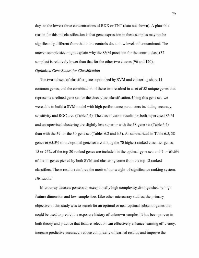
79
days to the lowest three concentrations of RDX or TNT (data not shown). A plausible
reason for this misclassification is that gene expression in these samples may not be
significantly different from that in the controls due to low levels of contaminant. The
uneven sample size might explain why the SVM precision for the control class (32
samples) is relatively lower than that for the other two classes (96 and 120).
Optimized Gene Subset for Classification
The two subsets of classifier genes optimized by SVM and clustering share 11
common genes, and the combination of these two resulted in a set of 58 unique genes that
represents a refined gene set for the three-class classification. Using this gene set, we
were able to build a SVM model with high performance parameters including accuracy,
sensitivity and ROC area (Table 6.4). The classification results for both supervised SVM
and unsupervised clustering are slightly less superior with the 58-gene set (Table 6.4)
than with the 39- or the 30-gene set (Tables 6.2 and 6.3). As summarized in Table 6.5, 38
genes or 65.5% of the optimal gene set are among the 70 highest ranked classifier genes,
15 or 75% of the top 20 ranked genes are included in the optimal gene set, and 7 or 63.6%
of the 11 genes picked by both SVM and clustering come from the top 12 ranked
classifiers. These results reinforce the merit of our weight-of-significance ranking system.
Discussion
Microarray datasets possess an exceptionally high complexity distinguished by high
feature dimension and low sample size. Like other microarray studies, the primary
objective of this study was to search for an optimal or near optimal subset of genes that
could be used to predict the exposure history of unknown samples. It has been proven in
both theory and practice that feature selection can effectively enhance learning efficiency,
increase predictive accuracy, reduce complexity of learned results, and improve the
80
Table 6.4
Confusion Matrix Showing Classification Results Using 58 Classifier Genes by SVM or
Clustering a
True Class(No. Samples)
No. Samples Classified as Accuracy (%) ROC AreaControl RDX TNT
SVM
Control (32) 26 6 0 81.3 0.936
RDX (120) 9 100 11 83.3 0.856
TNT (96) 2 13 81 84.4 0.913
Precision (%) 70.3 84.0 88.0
Weighted average (248) 83.8 (precision) 83.5 0.904
Clustering
Control (32)
a
22 1 9 68.8 NA
RDX (120) 48 55 17 45.8 NA
TNT (96) 22 10 64 66.7 NA
Precision (%) 23.9 83.3 71.1
Weighted average (248) 70.9 (precision) 56.9 NA
Note. Confusion matrix of classification results obtained using the refined set of 58 classifier genes combined from the SVM- and the
clustering-optimized gene sets. a ROC area was not computable with clustering.
accuracy of classification models [156, 160, 161]. Although numerous supervised or
unsupervised machine learning techniques have been used for feature selection and
sample classification of microarray data (for reviews see [162, 163, 164]), classification
performance appears to depend strongly on the dataset and less on the variable selection
and classification methods [165]. Meanwhile, it has been demonstrated that a combined
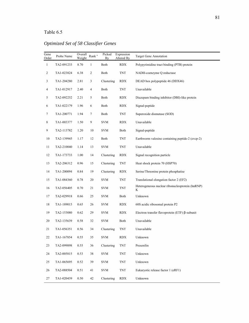
81
Table 6.5
Optimized Set of 58 Classifier Genes
Gene Order Probe Name Overall
Weight Rank a PickedBy
Expression Altered By Target Gene Annotation
1 TA2-091233 8.70 1 Both RDX Polypyrimidine tract binding (PTB) protein
2 TA1-023824 6.38 2 Both TNT NADH-coenzyme Q reductase
3 TA1-204280 2.81 3 Clustering RDX DEAD box polypeptide 46 (DDX46)
4 TA1-012917 2.40 4 Both TNT Unavailable
5 TA2-092252 2.21 5 Both RDX Diazepam binding inhibitor (DBI)-like protein
6 TA1-022179 1.96 6 Both RDX Signal-peptide
7 TA1-200771 1.94 7 Both TNT Superoxide dismutase (SOD)
8 TA1-003377 1.50 9 SVM RDX Unavailable
9 TA2-113782 1.20 10 SVM Both Signal-peptide
10 TA2-139945 1.17 12 Both TNT Earthworm valosine containing peptide-2 (evcp-2)
11 TA2-210040 1.14 13 SVM TNT Unavailable
12 TA1-173733 1.00 14 Clustering RDX Signal recognition particle
13 TA2-206312 0.96 15 Clustering TNT Heat shock protein 70 (HSP70)
14 TA1-200094 0.84 19 Clustering RDX Serine/Threonine protein phosphatise
15 TA1-084360 0.78 20 SVM TNT Translational elongation factor 2 (EF2)
16 TA2-056405 0.70 21 SVM TNT Heterogeneous nuclear ribonucleoprotein (hnRNP) K
17 TA2-029918 0.66 25 SVM Both Unknown
18 TA1-189015 0.65 26 SVM RDX 60S acidic ribosomal protein P2
19 TA2-153080 0.62 29 SVM RDX Electron transfer flavoprotein (ETF) -subunit
20 TA2-135639 0.58 32 SVM Both Unavailable
21 TA1-056351 0.56 34 Clustering TNT Unavailable
22 TA1-167854 0.55 35 SVM RDX Unknown
23 TA2-099898 0.55 36 Clustering TNT Presenilin
24 TA2-005815 0.53 38 SVM TNT Unknown
25 TA1-065695 0.52 39 SVM TNT Unknown
26 TA2-088504 0.51 41 SVM TNT Eukaryotic release factor 1 (eRF1)
27 TA1-020439 0.50 42 Clustering RDX Unknown
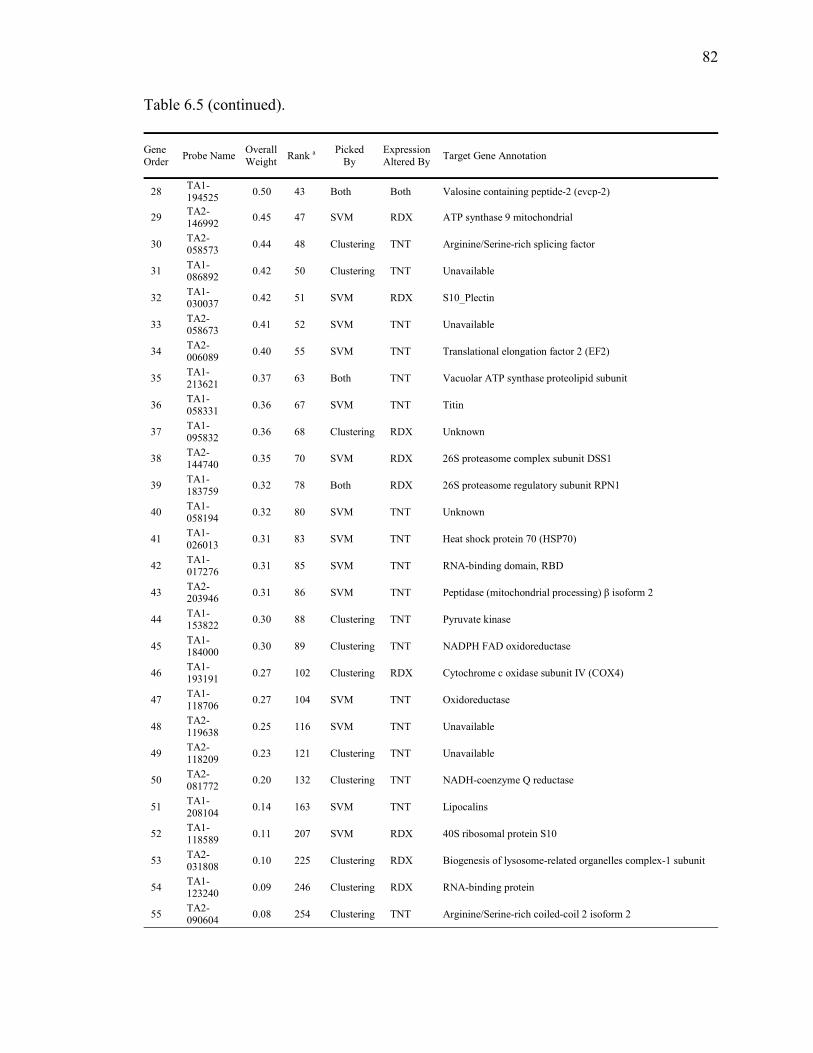
82
Table 6.5 (continued).
Gene Order Probe Name Overall
Weight Rank a PickedBy
Expression Altered By Target Gene Annotation
28 TA1-194525 0.50 43 Both Both Valosine containing peptide-2 (evcp-2)
29 TA2-146992 0.45 47 SVM RDX ATP synthase 9 mitochondrial
30 TA2-058573 0.44 48 Clustering TNT Arginine/Serine-rich splicing factor
31 TA1-086892 0.42 50 Clustering TNT Unavailable
32 TA1-030037 0.42 51 SVM RDX S10_Plectin
33 TA2-058673 0.41 52 SVM TNT Unavailable
34 TA2-006089 0.40 55 SVM TNT Translational elongation factor 2 (EF2)
35 TA1-213621 0.37 63 Both TNT Vacuolar ATP synthase proteolipid subunit
36 TA1-058331 0.36 67 SVM TNT Titin
37 TA1-095832 0.36 68 Clustering RDX Unknown
38 TA2-144740 0.35 70 SVM RDX 26S proteasome complex subunit DSS1
39 TA1-183759 0.32 78 Both RDX 26S proteasome regulatory subunit RPN1
40 TA1-058194 0.32 80 SVM TNT Unknown
41 TA1-026013 0.31 83 SVM TNT Heat shock protein 70 (HSP70)
42 TA1-017276 0.31 85 SVM TNT RNA-binding domain, RBD
43 TA2-203946 0.31 86 SVM TNT
44 TA1-153822 0.30 88 Clustering TNT Pyruvate kinase
45 TA1-184000 0.30 89 Clustering TNT NADPH FAD oxidoreductase
46 TA1-193191 0.27 102 Clustering RDX Cytochrome c oxidase subunit IV (COX4)
47 TA1-118706 0.27 104 SVM TNT Oxidoreductase
48 TA2-119638 0.25 116 SVM TNT Unavailable
49 TA2-118209 0.23 121 Clustering TNT Unavailable
50 TA2-081772 0.20 132 Clustering TNT NADH-coenzyme Q reductase
51 TA1-208104 0.14 163 SVM TNT Lipocalins
52 TA1-118589 0.11 207 SVM RDX 40S ribosomal protein S10
53 TA2-031808 0.10 225 Clustering RDX Biogenesis of lysosome-related organelles complex-1 subunit
54 TA1-123240 0.09 246 Clustering RDX RNA-binding protein
55 TA2-090604 0.08 254 Clustering TNT Arginine/Serine-rich coiled-coil 2 isoform 2
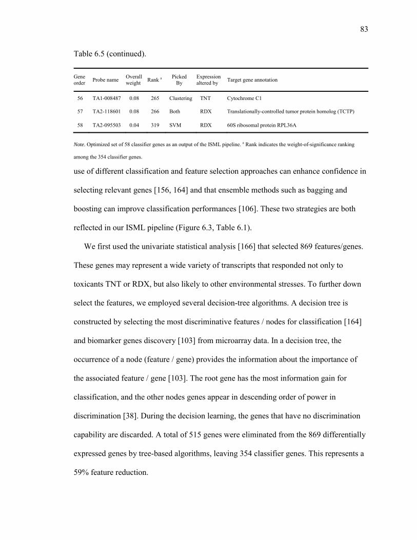
83
Table 6.5 (continued).
Gene order Probe name Overall
weight Rank a PickedBy
Expression altered by Target gene annotation
56 TA1-008487 0.08 265 Clustering TNT Cytochrome C1
57 TA2-118601 0.08 266 Both RDX Translationally-controlled tumor protein homolog (TCTP)
58 TA2-095503 0.04 319 SVM RDX 60S ribosomal protein RPL36A
Note. Optimized set of 58 classifier genes as an output of the ISML pipeline. a Rank indicates the weight-of-significance ranking
among the 354 classifier genes.
use of different classification and feature selection approaches can enhance confidence in
selecting relevant genes [156, 164] and that ensemble methods such as bagging and
boosting can improve classification performances [106]. These two strategies are both
reflected in our ISML pipeline (Figure 6.3, Table 6.1).
We first used the univariate statistical analysis [166] that selected 869 features/genes.
These genes may represent a wide variety of transcripts that responded not only to
toxicants TNT or RDX, but also likely to other environmental stresses. To further down
select the features, we employed several decision-tree algorithms. A decision tree is
constructed by selecting the most discriminative features / nodes for classification [164]
and biomarker genes discovery [103] from microarray data. In a decision tree, the
occurrence of a node (feature / gene) provides the information about the importance of
the associated feature / gene [103]. The root gene has the most information gain for
classification, and the other nodes genes appear in descending order of power in
discrimination [38]. During the decision learning, the genes that have no discrimination
capability are discarded. A total of 515 genes were eliminated from the 869 differentially
expressed genes by tree-based algorithms, leaving 354 classifier genes. This represents a
59% feature reduction.
84
As our goal was to scale down the size of potential classifier gene set while
maintaining a high discriminative power, we introduced in the ISML pipeline a new
algorithm to compute and rank the overall weight of the 354 individual classifier genes
based on their contribution/significance to classification. We also developed a novel
optimization algorithm for iteratively removing classifier genes that had little or a
negative impact on classification performance. This bottom-up removal process began
with the least important gene having the lowest overall weight. We chose to eliminate
those genes that only reduced the classification accuracies of all classes as well as the
weighted average. This conservative approach was adopted to preserve genes that might
increase the accuracy of one class but decrease that of another, like the 2nd, 5th, 7th, 9th,
11th and 13th genes in the clustering-optimized gene set (Figure 6.6b). These genes are
usually important for discriminating one particular class while confounding other classes.
SVMs are powerful classification models that have shown state-of-the-art
performance on several diagnosis and prognosis tasks on biological data [106, 167].
SVM-based classification can usually achieve higher accuracy/precision on a given
dataset than unsupervised algorithms. Ideally, an SVM analysis should produce a hyper-
plane that completely separates the feature vectors into non-overlapping groups.
However, perfect separation may not be possible, or it may result in a model with so
many feature vector dimensions that the model does not generalize well to other data,
which is a problem commonly known as over-fitting [168]. The risk of over-fitting to the
specific dataset in compensation for high accuracy/precision may render a high
probability of misclassification when the trained SVM model is applied to predict
unknown samples of other independent datasets. Unlike SVM, unsupervised learning
algorithms can overcome this shortfall with a trade-off of less superior

85
accuracy/precision. Our ISML pipeline adopted a compromise between these two
approaches. Although the effectiveness, efficiency and superiority of this approach has to
go through more stringent validation and testing, our results indicate that the final
combined gene set produced nearly as good classification outcome as the two separately
optimized gene subsets. This combined gene set need to be tested in field samples where
exposure history including species and concentration of contaminants as well as exposure
length is often unknown. Currently, a field soil study is undertaken to validate this
optimal gene set, where lab-cultured mature earthworms are exposed in field soils
primarily contaminated with TNT or RDX.
Classification accuracy was evaluated in this study on a sole basis of the pre-defined
exposure history, that is, each sample was labelled with a priori class corresponding to
the chemical it had been exposed to, disregarding the differences in soil concentration of
TNT or RDX. The accuracy of biological classification can be impaired for soils
containing low toxicant concentrations which may not induce gene expression effects
significant enough to distinguish exposed animals from the controls. This might
contribute partly to the lower accuracy obtained from clustering than from SVM. It is
desirable to define a threshold such as the lowest observable effect concentration
expressed as the toxicant concentration in soil or animals (body burden). We prefer body
burden as an exposure measure over soil concentration due to the often heterogeneous
distribution of toxicants in soil. This way, animals with a tissue concentration below the
threshold can be grouped/pre-defined together with unexposed control animals, which
potentially benefits clustering more than SVM.
To define a sensitive threshold, one can measure disease-related biological endpoints
that are presumably more sensitive than the mortality and growth endpoints in short-term
86
exposures of 4 or 14 days. Alternatively, one can measure toxicity-related phenotypic
(e.g., biochemical, physiological, or pathological) endpoints if a more toxicological
meaningful discrimination is desired. The SVM classification model for exposure
classification in the output of the ISML pipeline can be conveniently converted into a
disease or toxicity diagnosis model.
Another confounding factor that affects classification accuracy is that vulnerability
and susceptibility vary from one animal to another, which may be caused by many factors
such as genetic make-up, age, and physiological status. We believe that the diagnosis or
prediction accuracy of unknown samples can be greatly improved if gene expression
profiles of biologically well-characterized, pre-defined animals are used as the training
dataset, just like in cancer microarray studies.
Among the 58 optimized genes, 93% genes exhibited toxicant-specific gene
expression alterations, that is, 32 genes responded specifically to TNT, 22 to RDX, and
only 4 to both chemicals (Table 6.5). Forty-two genes (72%) have meaningful annotation
with a wide range of biological functions spanning from antioxidant response (COX4 and
NADH-coenzyme Q reductase) to spermatogenesis (evcp-2) and GABA receptor
modulator (DBI, also known as Acyl-CoA-binding protein or ACBP). Three of the top 10
ranked genes, PTB, DBI and SOD, have previously been shown being altered by TNT
[157] or RDX [158]. Two probes targeting two highly similar transcripts coding for evcp-
2, a gene expressed specifically in the anterior segments of sexually mature earthworms
[169], take the 10th and the 28th positions on the optimal gene list, suggesting that both
TNT and RDX may affect spermatogenesis. On the list, there are also several stress-
responding genes such as HSP70 (#13 & #41) [170] as well as cancer-related genes such
as TCTP (#57) [171]. It is worth noting that six genes, PTB (#1) [172], DDX46 (#3)
87
[173], EF2 (#15 & #34) [174], hnRNP K (#16) [175], and eRF1 (# 26) [176] are all
involved in mRNA splicing or processing and RNA translation initiation or termination,
indicating alteration of mRNA secondary structure and protein synthesis may be targeted
by both TNT and RDX. More work should be devoted to exploring biological functions
and interactions of the 58 genes that may lead or be linked to toxicological effects or
biochemical endpoints.
This study addresses a sophisticated issue of discovering and optimizing classifier
gene sets in environmentally relevant animal models. Although a perfect or the best
solution to it is yet to be found, we have demonstrated that the ISML pipeline can reduce
the dimensionality of microarray datasets, identify and rank classifier genes, generate a
small set of classifier genes, produce an SVM classification model with high accuracy,
and select a small group of biomarker candidate genes for biological validation. This
approach can also be applied to discover diagnostic biomarker genes exhibiting toxicity-
or disease-dependent response in environmental species from fish and springtail to water
flea and earthworm.
We report here some preliminary results of a much larger effort. Our future work
include: (1) compare the performance of the ISML approach with that of other popular
and existing feature selection techniques such as SVM-RFE (SVM Recursive Feature
2 using the earthworm
dataset and other microarray datasets; (2) validate the final 58- gene set using other
experimental methods such as real-time quantitative PCR; (3) further test the classifiers
in field samples; (4) identify TNT/RDX concentration-related classifier genes; and (5)
validate the biochemical outcome regulated by the biomarker candidate genes. We
88
believe that these consorted efforts will lead us to discovery of novel classifier genes
useful for environmental risk assessment.
Time-Series Earthworm Microarray Dataset
Experimental Design and Dataset Generation
The following experiment id designed and conducted by Dr. Ping Gong at the
Environmental Laboratory of U.S. Army Engineer Research and Development Center. A
new earthworm array containing 43,803 non-redundant 60-mer probes was used to
generate the dataset. The probes were selected from 63,641 previously validated
oligonucleotide probes, each targeting a unique Eisenia fetida transcript, and 37,439
(59%) of probed targets had meaningful biological annotation [157]. A synchronized
earthworm culture (starting from cocoons) was created and mature worms bearing
clitellum and weighing 0.4~0.6 g were chosen for this experiment. Each worm was
transferred from artificial soil-based bedding (culture) and housed in an individual glass
vial (115 mL in volume) [177]. These worms were exposed to carbaryl (20 ng/cm2) or
RDX (2 μg/cm2) or acetone (solvent control) on moistened filter paper lined up inside the
vial. These chemical concentrations were selected because they did not cause lethality
(based on results from preliminary tests). The entire experiment was divided into three
phases (Figure 6.8): acclimation (4 days), exposure (6 days) and recovery (7 days). The
acclimation phase was necessary for the worms to adapt from soil culture to filter paper,
and four samplings were taken to establish the “background” baseline under the control
condition. Worms were sampled at 13 and 14 time points for all three treatments (control,
RDX and carbaryl) during the exposure and the recovery phase, respectively. Sampled
worms were measured for conduction velocity of the medial giant nerve fiber (MGF)
before being sacrificed by snap-freezing in liquid nitrogen. All yet-to-be-sampled worms
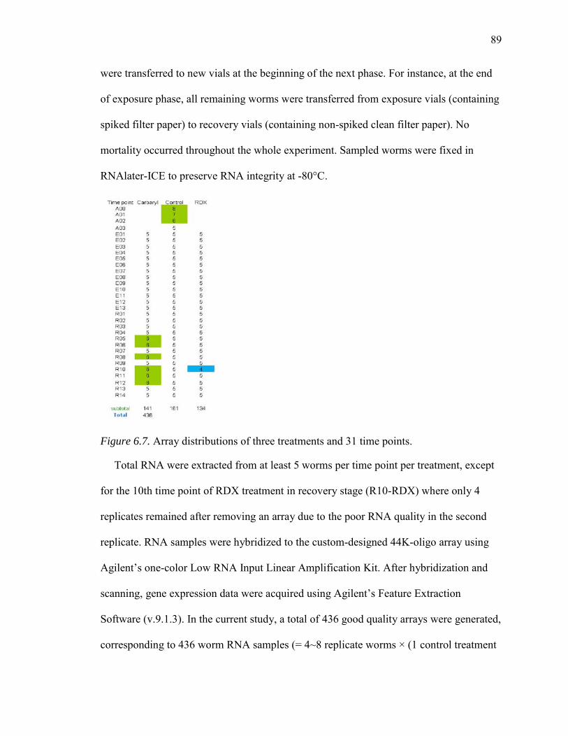
89
were transferred to new vials at the beginning of the next phase. For instance, at the end
of exposure phase, all remaining worms were transferred from exposure vials (containing
spiked filter paper) to recovery vials (containing non-spiked clean filter paper). No
mortality occurred throughout the whole experiment. Sampled worms were fixed in
RNAlater-ICE to preserve RNA integrity at -80°C.
Figure 6.7. Array distributions of three treatments and 31 time points.
Total RNA were extracted from at least 5 worms per time point per treatment, except
for the 10th time point of RDX treatment in recovery stage (R10-RDX) where only 4
replicates remained after removing an array due to the poor RNA quality in the second
replicate. RNA samples were hybridized to the custom-designed 44K-oligo array using
Agilent’s one-color Low RNA Input Linear Amplification Kit. After hybridization and
scanning, gene expression data were acquired using Agilent’s Feature Extraction
Software (v.9.1.3). In the current study, a total of 436 good quality arrays were generated,
corresponding to 436 worm RNA samples (= 4~8 replicate worms × (1 control treatment
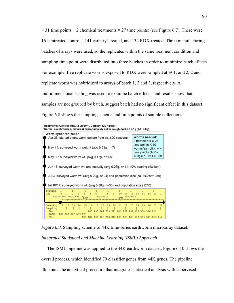
90
× 31 time points + 2 chemical treatments × 27 time points) (see Figure 6.7). There were
161 untreated controls, 141 carbaryl-treated, and 134 RDX-treated. Three manufacturing
batches of arrays were used, so the replicates within the same treatment condition and
sampling time point were distributed into three batches in order to minimize batch effects.
For example, five replicate worms exposed to RDX were sampled at E01, and 2, 2 and 1
replicate worm was hybridized to arrays of batch 1, 2 and 3, respectively. A
multidimensional scaling was used to examine batch effects, and results show that
samples are not grouped by batch, suggest batch had no significant effect in this dataset.
Figure 6.8 shows the sampling scheme and time points of sample collections.
Figure 6.8. Sampling scheme of 44K time-series earthworm microarray dataset.
Integrated Statistical and Machine Learning (ISML) Approach
The ISML pipeline was applied to the 44K earthworm dataset. Figure 6.10 shows the
overall process, which identified 70 classifier genes from 44K genes. The pipeline
illustrates the analytical procedure that integrates statistical analysis with supervised
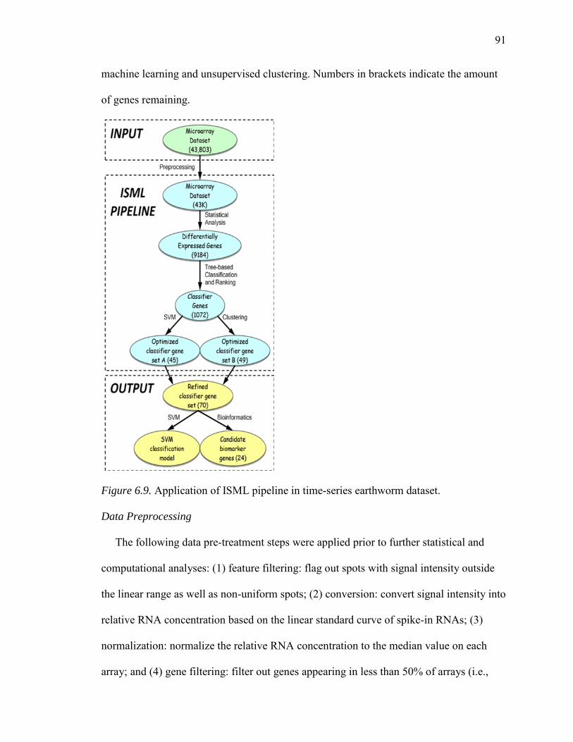
91
machine learning and unsupervised clustering. Numbers in brackets indicate the amount
of genes remaining.
Figure 6.9. Application of ISML pipeline in time-series earthworm dataset.
Data Preprocessing
The following data pre-treatment steps were applied prior to further statistical and
computational analyses: (1) feature filtering: flag out spots with signal intensity outside
the linear range as well as non-uniform spots; (2) conversion: convert signal intensity into
relative RNA concentration based on the linear standard curve of spike-in RNAs; (3)
normalization: normalize the relative RNA concentration to the median value on each
array; and (4) gene filtering: filter out genes appearing in less than 50% of arrays (i.e.,
92
present on at least 219 arrays). There were more than 43,000 genes remaining after this
procedure.
Feature Filtering by Univariate Statistical Analysis
The Class Comparison Between Groups of Arrays Tool in BRB-ArrayTools v.3.8
software package ([103]) was used to identify significantly changed genes. The collated
earthworm array dataset was imported without any further normalization or
transformation. The tool runs a random variance version of the t-test or F-test separately
for each gene. It performs random permutations of the class labels and computes the
proportion of the random permutations that give as many genes significant at the level set
by the user as are found in comparing the true class labels. The following class-
comparison analyses were conducted to infer genes differentially expressed in response
to Carbaryl or RDX: two 2-class comparisons: pooled controls vs. pooled Carbaryl or
RDX treatments. The following settings were employed: a univariate test random
variance model, multivariate permutation tests with 10,000 random permutations, a
confidence level of false discovery rate assessment = 99%, and a maximum allowed
number of false-positive genes = 10. A total of 9184 unique genes were obtained after
combining all significantly changed gene lists from Carbaryl- and RDX-exposures. The
frequency of changes of gene expression values for each gene across 31 time points are
counted, and among the 9184 differentially expressed genes (DEGs), 2574 unique genes
were identified as DEGs for at least two time points.
Identification and Optimization of Classifier Genes
Classifier Gene Selection and Ranking
We used seven different tree-based machine learning algorithms to select classifier
genes from the 2574 statistically significant genes. Each algorithm in combination with
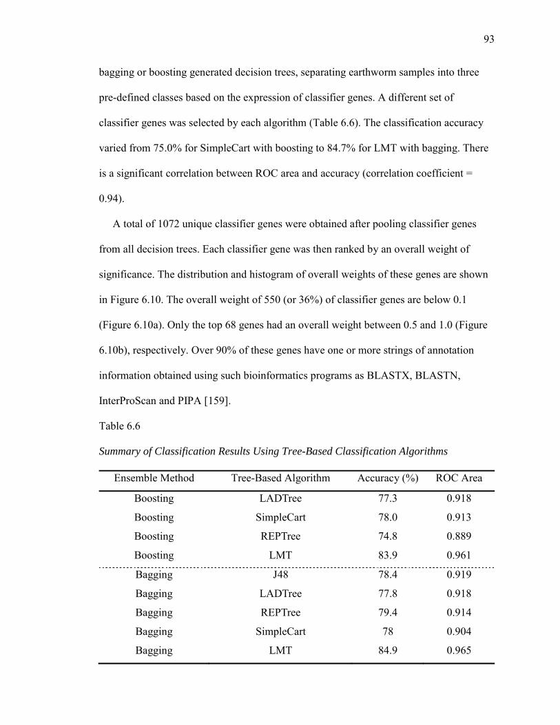
93
bagging or boosting generated decision trees, separating earthworm samples into three
pre-defined classes based on the expression of classifier genes. A different set of
classifier genes was selected by each algorithm (Table 6.6). The classification accuracy
varied from 75.0% for SimpleCart with boosting to 84.7% for LMT with bagging. There
is a significant correlation between ROC area and accuracy (correlation coefficient =
0.94).
A total of 1072 unique classifier genes were obtained after pooling classifier genes
from all decision trees. Each classifier gene was then ranked by an overall weight of
significance. The distribution and histogram of overall weights of these genes are shown
in Figure 6.10. The overall weight of 550 (or 36%) of classifier genes are below 0.1
(Figure 6.10a). Only the top 68 genes had an overall weight between 0.5 and 1.0 (Figure
6.10b), respectively. Over 90% of these genes have one or more strings of annotation
information obtained using such bioinformatics programs as BLASTX, BLASTN,
InterProScan and PIPA [159].
Table 6.6
Summary of Classification Results Using Tree-Based Classification Algorithms
Ensemble Method Tree-Based Algorithm Accuracy (%) ROC Area
Boosting LADTree 77.3 0.918
Boosting SimpleCart 78.0 0.913
Boosting REPTree 74.8 0.889
Boosting LMT 83.9 0.961
Bagging J48 78.4 0.919
Bagging LADTree 77.8 0.918
Bagging REPTree 79.4 0.914
Bagging SimpleCart 78 0.904
Bagging LMT 84.9 0.965

94
(a) (b)
Figure 6.10. The accumulative distribution (a) and histogram (b) of weights of 1074classifier genes. In the histogram, the bin size is set at 0.02.
Refinement of Classifier Gene Set Using MC-SVM or Clustering
Two different algorithms, SMO and K-mean clustering, were employed to optimize
the number and set of genes from the 1074 ranked classifier genes. Composition of the
classifier gene set had a significant influence on classification accuracy (Figure 6.11).
Using SMO, as few as 22 top ranked genes classified 82% of the 436 samples into correct
classes (Figure 6.11a). Starting at the 268th gene, the inclusion of additional classifier
genes not only did not improve the classification accuracy for the TNT and the RDX
classes as well as the weighted average accuracy, but deteriorated the accuracy for the
control class (Figure 6.11a). Similarly, with the clustering approach, the top ranked 23
genes correctly clustered 72% of the samples, while addition of other genes did little, if
any, to improve the accuracy of either individual classes or the weighted average (Figure
6.11b). Clearly, individual classifier genes vary remarkably in its contribution to the
change of classification accuracy, which also depends on the choice of machine learning
algorithms. In Figure 6.11, the weighted average accuracy and the accuracy for each of
the three classes (control, RDX and Carbaryl) are shown for each set of genes (1~1074
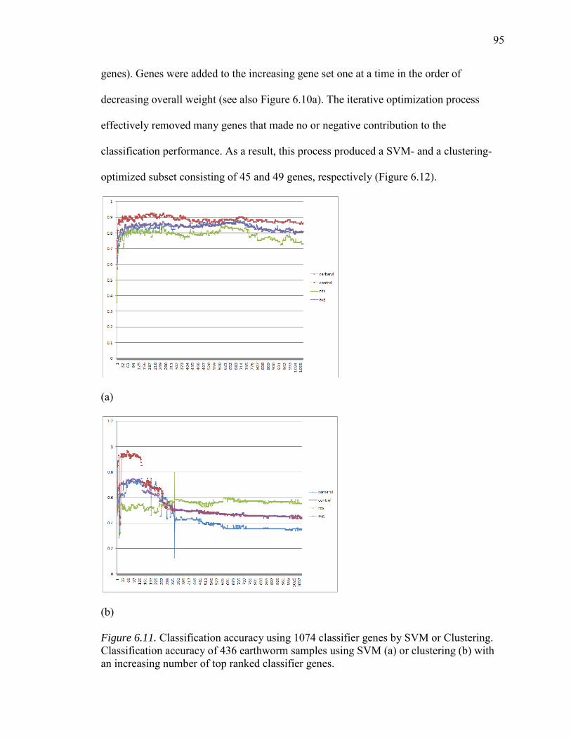
95
genes). Genes were added to the increasing gene set one at a time in the order of
decreasing overall weight (see also Figure 6.10a). The iterative optimization process
effectively removed many genes that made no or negative contribution to the
classification performance. As a result, this process produced a SVM- and a clustering-
optimized subset consisting of 45 and 49 genes, respectively (Figure 6.12).
(a)
(b)
Figure 6.11. Classification accuracy using 1074 classifier genes by SVM or Clustering. Classification accuracy of 436 earthworm samples using SVM (a) or clustering (b) with an increasing number of top ranked classifier genes.
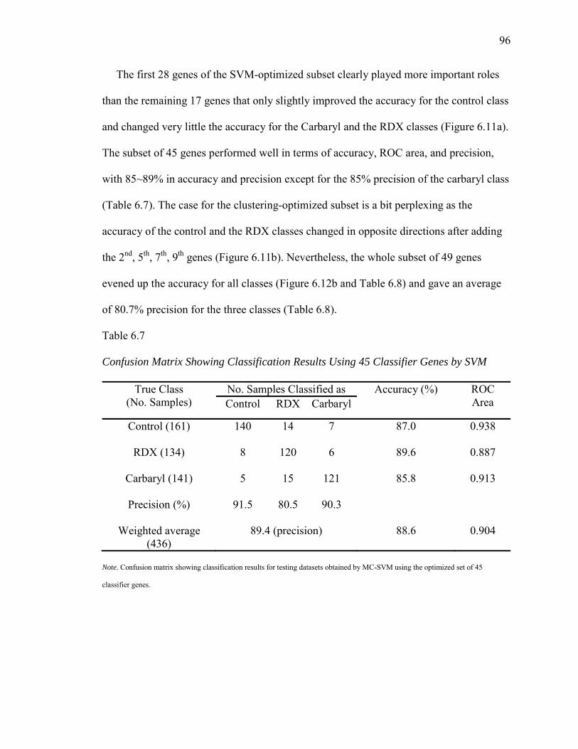
96
The first 28 genes of the SVM-optimized subset clearly played more important roles
than the remaining 17 genes that only slightly improved the accuracy for the control class
and changed very little the accuracy for the Carbaryl and the RDX classes (Figure 6.11a).
The subset of 45 genes performed well in terms of accuracy, ROC area, and precision,
with 85~89% in accuracy and precision except for the 85% precision of the carbaryl class
(Table 6.7). The case for the clustering-optimized subset is a bit perplexing as the
accuracy of the control and the RDX classes changed in opposite directions after adding
the 2nd, 5th, 7th, 9th genes (Figure 6.11b). Nevertheless, the whole subset of 49 genes
evened up the accuracy for all classes (Figure 6.12b and Table 6.8) and gave an average
of 80.7% precision for the three classes (Table 6.8).
Table 6.7
Confusion Matrix Showing Classification Results Using 45 Classifier Genes by SVM
True Class(No. Samples)
No. Samples Classified as Accuracy (%) ROC AreaControl RDX Carbaryl
Control (161) 140 14 7 87.0 0.938
RDX (134) 8 120 6 89.6 0.887
Carbaryl (141) 5 15 121 85.8 0.913
Precision (%) 91.5 80.5 90.3
Weighted average (436)
89.4 (precision) 88.6 0.904
Note. Confusion matrix showing classification results for testing datasets obtained by MC-SVM using the optimized set of 45
classifier genes.
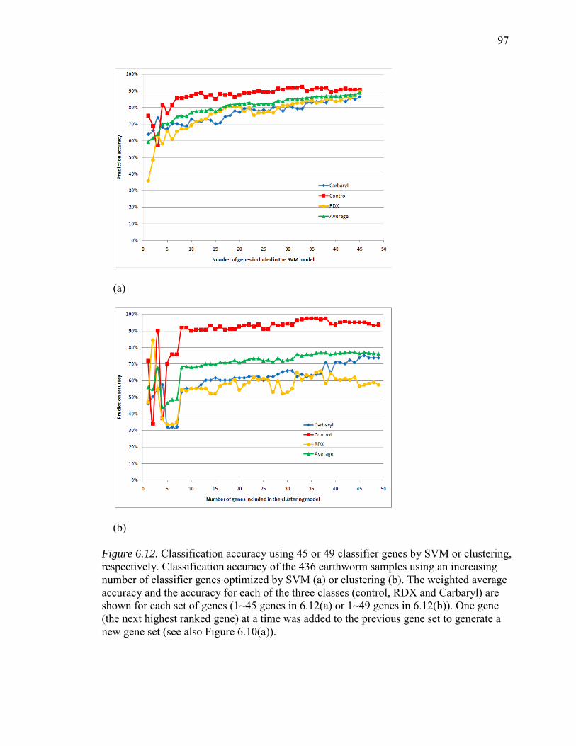
97
(a)
(b)
Figure 6.12. Classification accuracy using 45 or 49 classifier genes by SVM or clustering, respectively. Classification accuracy of the 436 earthworm samples using an increasing number of classifier genes optimized by SVM (a) or clustering (b). The weighted average accuracy and the accuracy for each of the three classes (control, RDX and Carbaryl) are shown for each set of genes (1~45 genes in 6.12(a) or 1~49 genes in 6.12(b)). One gene (the next highest ranked gene) at a time was added to the previous gene set to generate a new gene set (see also Figure 6.10(a)).
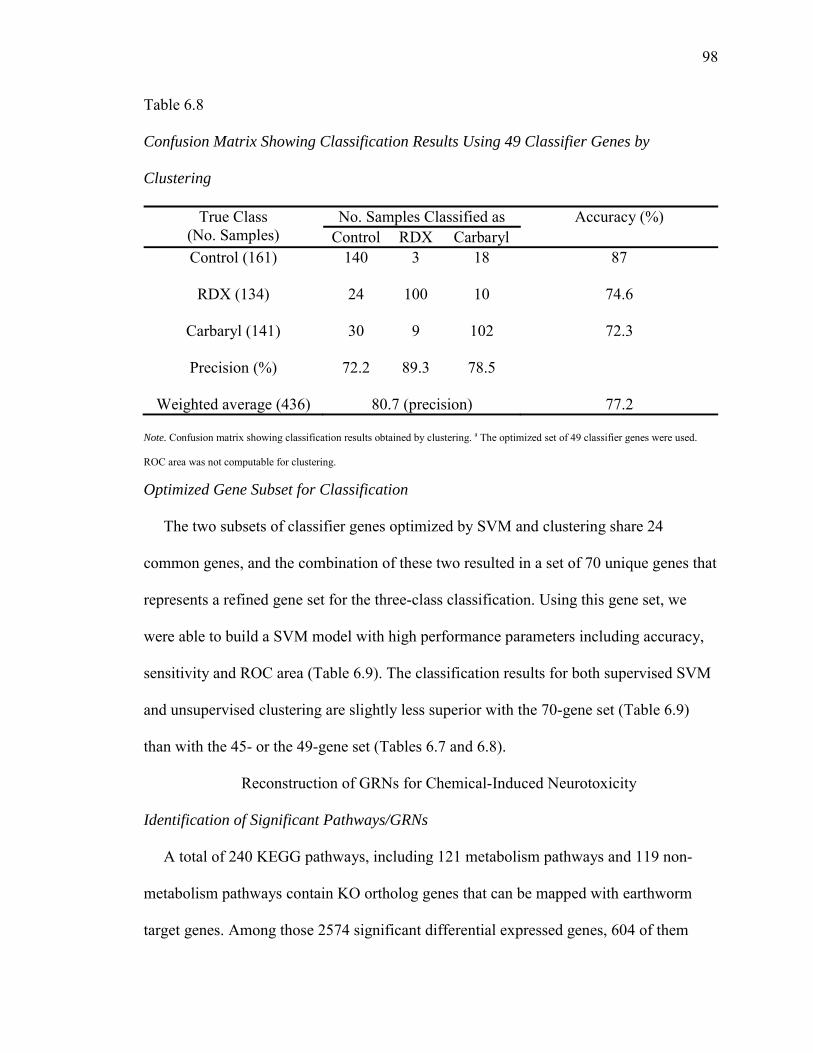
98
Table 6.8
Confusion Matrix Showing Classification Results Using 49 Classifier Genes by
Clustering
True Class(No. Samples)
No. Samples Classified as Accuracy (%)Control RDX Carbaryl
Control (161) 140 3 18 87
RDX (134) 24 100 10 74.6
Carbaryl (141) 30 9 102 72.3
Precision (%) 72.2 89.3 78.5
Weighted average (436) 80.7 (precision) 77.2
Note. Confusion matrix showing classification results obtained by clustering. a The optimized set of 49 classifier genes were used.
ROC area was not computable for clustering.
Optimized Gene Subset for Classification
The two subsets of classifier genes optimized by SVM and clustering share 24
common genes, and the combination of these two resulted in a set of 70 unique genes that
represents a refined gene set for the three-class classification. Using this gene set, we
were able to build a SVM model with high performance parameters including accuracy,
sensitivity and ROC area (Table 6.9). The classification results for both supervised SVM
and unsupervised clustering are slightly less superior with the 70-gene set (Table 6.9)
than with the 45- or the 49-gene set (Tables 6.7 and 6.8).
Reconstruction of GRNs for Chemical-Induced Neurotoxicity
Identification of Significant Pathways/GRNs
A total of 240 KEGG pathways, including 121 metabolism pathways and 119 non-
metabolism pathways contain KO ortholog genes that can be mapped with earthworm
target genes. Among those 2574 significant differential expressed genes, 604 of them
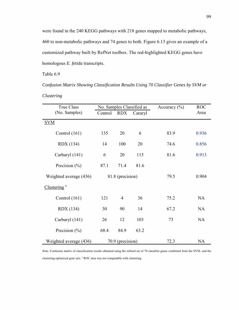
99
were found in the 240 KEGG pathways with 218 genes mapped to metabolic pathways,
460 to non-metabolic pathways and 74 genes to both. Figure 6.13 gives an example of a
customized pathway built by RefNet toolbox. The red-highlighted KEGG genes have
homologous E. fetida transcripts.
Table 6.9
Confusion Matrix Showing Classification Results Using 70 Classifier Genes by SVM or
Clustering
True Class(No. Samples)
No. Samples Classified as Accuracy (%) ROC AreaControl RDX Cararyl
SVM
Control (161) 135 20 6 83.9 0.936
RDX (134) 14 100 20 74.6 0.856
Carbaryl (141) 6 20 115 81.6 0.913
Precision (%) 87.1 71.4 81.6
Weighted average (436) 81.8 (precision) 79.5 0.904
Clustering
Control (161)
a
121 4 36 75.2 NA
RDX (134) 30 90 14 67.2 NA
Carbaryl (141) 26 12 103 73 NA
Precision (%) 68.4 84.9 63.2
Weighted average (436) 70.9 (precision) 72.3 NA
Note. Confusion matrix of classification results obtained using the refined set of 70 classifier genes combined from the SVM- and the
clustering-optimized gene sets. a ROC area was not computable with clustering.
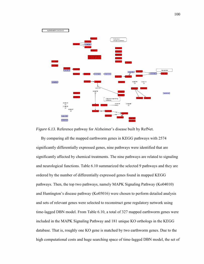
100
Figure 6.13. Reference pathway for Alzheimer’s disease built by RefNet.
By comparing all the mapped earthworm genes in KEGG pathways with 2574
significantly differentially expressed genes, nine pathways were identified that are
significantly affected by chemical treatments. The nine pathways are related to signaling
and neurological functions. Table 6.10 summarized the selected 9 pathways and they are
ordered by the number of differentially expressed genes found in mapped KEGG
pathways. Then, the top two pathways, namely MAPK Signaling Pathway (Ko04010)
and Huntington’s disease pathway (Ko05016) were chosen to perform detailed analysis
and sets of relevant genes were selected to reconstruct gene regulatory network using
time-lagged DBN model. From Table 6.10, a total of 327 mapped earthworm genes were
included in the MAPK Signaling Pathway and 181 unique KO orthologs in the KEGG
database. That is, roughly one KO gene is matched by two earthworm genes. Due to the
high computational costs and huge searching space of time-lagged DBN model, the set of
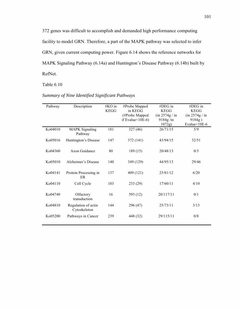
101
372 genes was difficult to accomplish and demanded high performance computing
facility to model GRN. Therefore, a part of the MAPK pathway was selected to infer
GRN, given current computing power. Figure 6.14 shows the reference networks for
MAPK Signaling Pathway (6.14a) and Huntington’s Disease Pathway (6.14b) built by
RefNet.
Table 6.10
Summary of Nine Identified Significant Pathways
Pathway Description #KO in KEGG
#Probe Mapped in KEGG
(#Probe Mapped if Evalue<10E-6)
#DEG in KEGG
(in 2574g / in 9184g /in 1072g)
#DEG in KEGG
(in 2574g / in 9184g )
Evalue<10E-6Ko04010 MAPK Signaling
Pathway181 327 (46) 26/71/15 5/9
Ko05016 Huntington’s Disease 147 372 (141) 43/94/15 32/51
Ko04360 Axon Guidance 80 189 (15) 20/48/13 0/3
Ko05010 Alzheimer’s Disease 140 349 (129) 44/95/13 29/46
Ko04141 Protein Processing in ER
137 409 (121) 25/81/12 6/20
Ko04110 Cell Cycle 103 233 (29) 17/60/11 4/10
Ko04740 Olfactory transduction
16 593 (12) 20/117/11 0/1
Ko04810 Regulation of actin Cytoskeleton
144 296 (47) 25/73/11 3/13
Ko05200 Pathways in Cancer 239 448 (32) 29/115/11 0/8
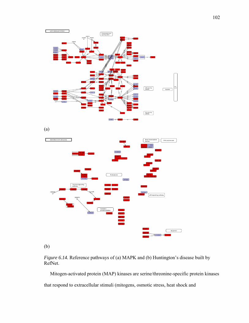
102
(a)
(b)
Figure 6.14. Reference pathways of (a) MAPK and (b) Huntington’s disease built by RefNet.
Mitogen-activated protein (MAP) kinases are serine/threonine-specific protein kinases
that respond to extracellular stimuli (mitogens, osmotic stress, heat shock and
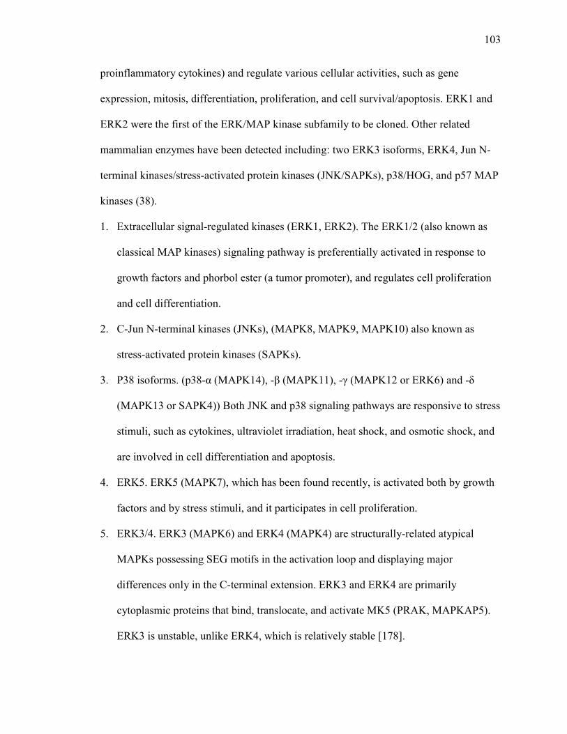
103
proinflammatory cytokines) and regulate various cellular activities, such as gene
expression, mitosis, differentiation, proliferation, and cell survival/apoptosis. ERK1 and
ERK2 were the first of the ERK/MAP kinase subfamily to be cloned. Other related
mammalian enzymes have been detected including: two ERK3 isoforms, ERK4, Jun N-
terminal kinases/stress-activated protein kinases (JNK/SAPKs), p38/HOG, and p57 MAP
kinases (38).
1. Extracellular signal-regulated kinases (ERK1, ERK2). The ERK1/2 (also known as
classical MAP kinases) signaling pathway is preferentially activated in response to
growth factors and phorbol ester (a tumor promoter), and regulates cell proliferation
and cell differentiation.
2. C-Jun N-terminal kinases (JNKs), (MAPK8, MAPK9, MAPK10) also known as
stress-activated protein kinases (SAPKs).
3. P38 isoforms. (p38- - - -
(MAPK13 or SAPK4)) Both JNK and p38 signaling pathways are responsive to stress
stimuli, such as cytokines, ultraviolet irradiation, heat shock, and osmotic shock, and
are involved in cell differentiation and apoptosis.
4. ERK5. ERK5 (MAPK7), which has been found recently, is activated both by growth
factors and by stress stimuli, and it participates in cell proliferation.
5. ERK3/4. ERK3 (MAPK6) and ERK4 (MAPK4) are structurally-related atypical
MAPKs possessing SEG motifs in the activation loop and displaying major
differences only in the C-terminal extension. ERK3 and ERK4 are primarily
cytoplasmic proteins that bind, translocate, and activate MK5 (PRAK, MAPKAP5).
ERK3 is unstable, unlike ERK4, which is relatively stable [178].
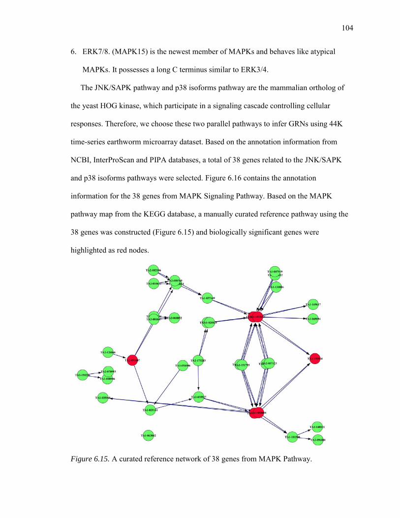
104
6. ERK7/8. (MAPK15) is the newest member of MAPKs and behaves like atypical
MAPKs. It possesses a long C terminus similar to ERK3/4.
The JNK/SAPK pathway and p38 isoforms pathway are the mammalian ortholog of
the yeast HOG kinase, which participate in a signaling cascade controlling cellular
responses. Therefore, we choose these two parallel pathways to infer GRNs using 44K
time-series earthworm microarray dataset. Based on the annotation information from
NCBI, InterProScan and PIPA databases, a total of 38 genes related to the JNK/SAPK
and p38 isoforms pathways were selected. Figure 6.16 contains the annotation
information for the 38 genes from MAPK Signaling Pathway. Based on the MAPK
pathway map from the KEGG database, a manually curated reference pathway using the
38 genes was constructed (Figure 6.15) and biologically significant genes were
highlighted as red nodes.
Figure 6.15. A curated reference network of 38 genes from MAPK Pathway.
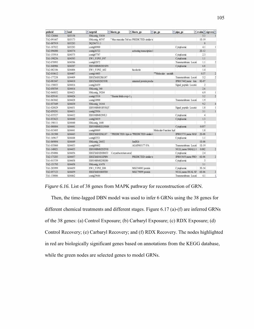
105
Figure 6.16. List of 38 genes from MAPK pathway for reconstruction of GRN.
Then, the time-lagged DBN model was used to infer 6 GRNs using the 38 genes for
different chemical treatments and different stages. Figure 6.17 (a)-(f) are inferred GRNs
of the 38 genes: (a) Control Exposure; (b) Carbaryl Exposure; (c) RDX Exposure; (d)
Control Recovery; (e) Carbaryl Recovery; and (f) RDX Recovery. The nodes highlighted
in red are biologically significant genes based on annotations from the KEGG database,
while the green nodes are selected genes to model GRNs.
probeid koid targetid blastn_go blastx_go ips_go pipa_go evalue sigeventTA2-126866 K03158 SMcontig_53030 5.3 1TA2-091607 K03173 SMcontig_40747 " Mus musculus Tnf recePREDICTED: similar to 1E-19TA1-007919 K03283 DQ286711.1 0TA1-107832 K03283 contig00900 Cytoplasmic 4.1 1TA2-096080 K04374 contig26722 activating transcription fa 2E-12TA1-155914 K04375 contig07787 Cytoplasmic 2.3TA1-190236 K04383 EW1_F1P03_F07 Cytoplasmic 1.1TA2-070993 K04386 contig02072 Transmembrane Locatio 1.1 2TA1-048906 K04387 EB3O8BM02H1SF8 Cytoplasmic 6.8TA2-082186 K04406 EW1_F1P02_A02 fucolectin 1.4TA2-010612 K04407 contig14403 """Molecular Function: m 0.37 2TA1-177238 K04409 EB3ZX6E02JKG87 Transmembrane Locatio 5.2 2TA2-081847 K04410 EB3ZX6E02H35FR unnamed protein produc IPR017442;name kina 8E-07TA1-158033 K04416 contig26439 Signal_peptide Location 2TA2-050769 K04416 SMcontig_340 2.6TA2-068852 K04421 SMcontig_39284 6.9 1TA1-029141 K04426 contig15518 " Eisenia fetida evcp-1 g 5.2 2TA1-063042 K04428 contig24900 Transmembrane Locatio 1.9TA1-037449 K04430 SMcontig_16164 9.2 4TA1-028829 K04431 EB3O8BM01BYSQT Signal_peptide Location 1.8 1TA2-059291 K04431 contig25936 3.1 1TA2-035527 K04432 EB3O8BM02I9JL3 Cytoplasmic 4TA1-033623 K04440 contig24419 Cytoplasmic 1.3TA1-190111 K04440 SMcontig_1640 7TA1-088084 K04441 EB3O8BM02G38M8 Cytoplasmic 0.057TA1-015495 K04441 contig08069 Molecular Function: hydr 1.8TA1-181500 K04443 EB3ZX6E02JKLS7 " PREDICTED: Apis me"PREDICTED: similar to IPR015731;name MAP 2E-08 1TA1-169617 K04448 contig02521 Cytoplasmic 1.1TA1-069894 K04449 SMcontig_24452 JunDLb 1E-08TA1-035060 K04453 contig00402 AGAP003177-PA Transmembrane Locatio 1E-19TA1-148021 K04455 EB3O8BM02I5ZVH NULL;name SMALL H 0.002 2TA1-054006 K04456 EB3ZX6E02HBMTJ Corynebacterium urealy Cytoplasmic 2.4TA2-173283 K04457 EB3ZX6E01EEPBN PREDICTED: similar to IPR015655;name PROT 6E-06 2TA1-015759 K04458 EB3O8BM02JRER0 Cytoplasmic 3TA2-151795 K04458 SMcontig_61478 3.1TA1-203999 K04459 EW1_F1P02_E08 MGC84083 protein Cytoplasmic 3E-34TA2-057123 K04459 EB3ZX6E01BHTE0 MGC79099 protein NULL;name DUAL SP 6E-06 2TA1-130886 K04462 contig29646 Transmembrane Locatio 4.1 1
eee ttttttt
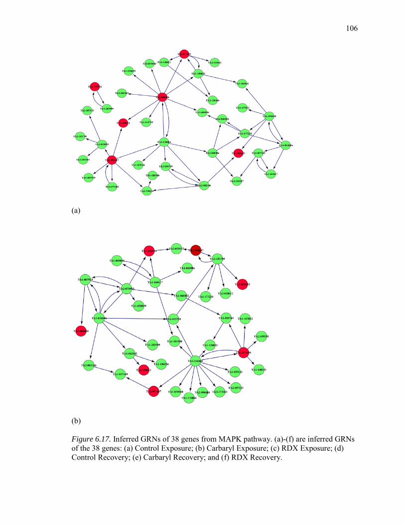
106
(a)
(b)
Figure 6.17. Inferred GRNs of 38 genes from MAPK pathway. (a)-(f) are inferred GRNs of the 38 genes: (a) Control Exposure; (b) Carbaryl Exposure; (c) RDX Exposure; (d) Control Recovery; (e) Carbaryl Recovery; and (f) RDX Recovery.
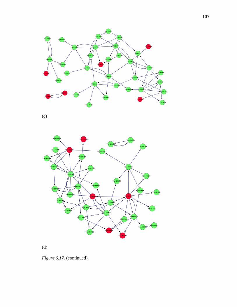
107
(c)
(d)
Figure 6.17. (continued).
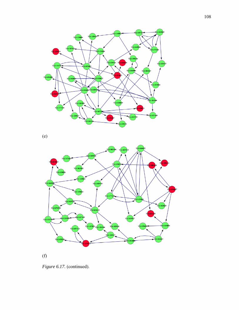
108
(e)
(f)
Figure 6.17. (continued).
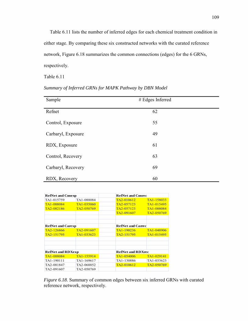
109
Table 6.11 lists the number of inferred edges for each chemical treatment condition in
either stage. By comparing these six constructed networks with the curated reference
network, Figure 6.18 summarizes the common connections (edges) for the 6 GRNs,
respectively.
Table 6.11
Summary of Inferred GRNs for MAPK Pathway by DBN Model
Sample # Edges Inferred
Refnet 62
Control, Exposure 55
Carbaryl, Exposure 49
RDX, Exposure 61
Control, Recovery 63
Carbaryl, Recovery 69
RDX, Recovery 60
Figure 6.18. Summary of common edges between six inferred GRNs with curated reference network, respectively.
RefNet and Conexp RefNet and ConrecTA1-015759 TA1-088084 TA2-010612 TA1-158033TA1-088084 TA1-035060 TA2-057123 TA1-015495TA2-082186 TA2-050769 TA2-057123 TA1-088084
TA2-091607 TA2-050769
RefNet and Carexp RefNet and CarrecTA2-126866 TA2-091607 TA1-190236 TA1-048906TA2-151795 TA1-033623 TA2-151795 TA1-015495
RefNet and RDXexp RefNet and RDXrecTA1-088084 TA1-155914 TA1-054006 TA1-029141TA1-190111 TA1-169617 TA1-130886 TA1-033623TA2-081847 TA2-068852 TA2-010612 TA2-050769TA2-091607 TA2-050769
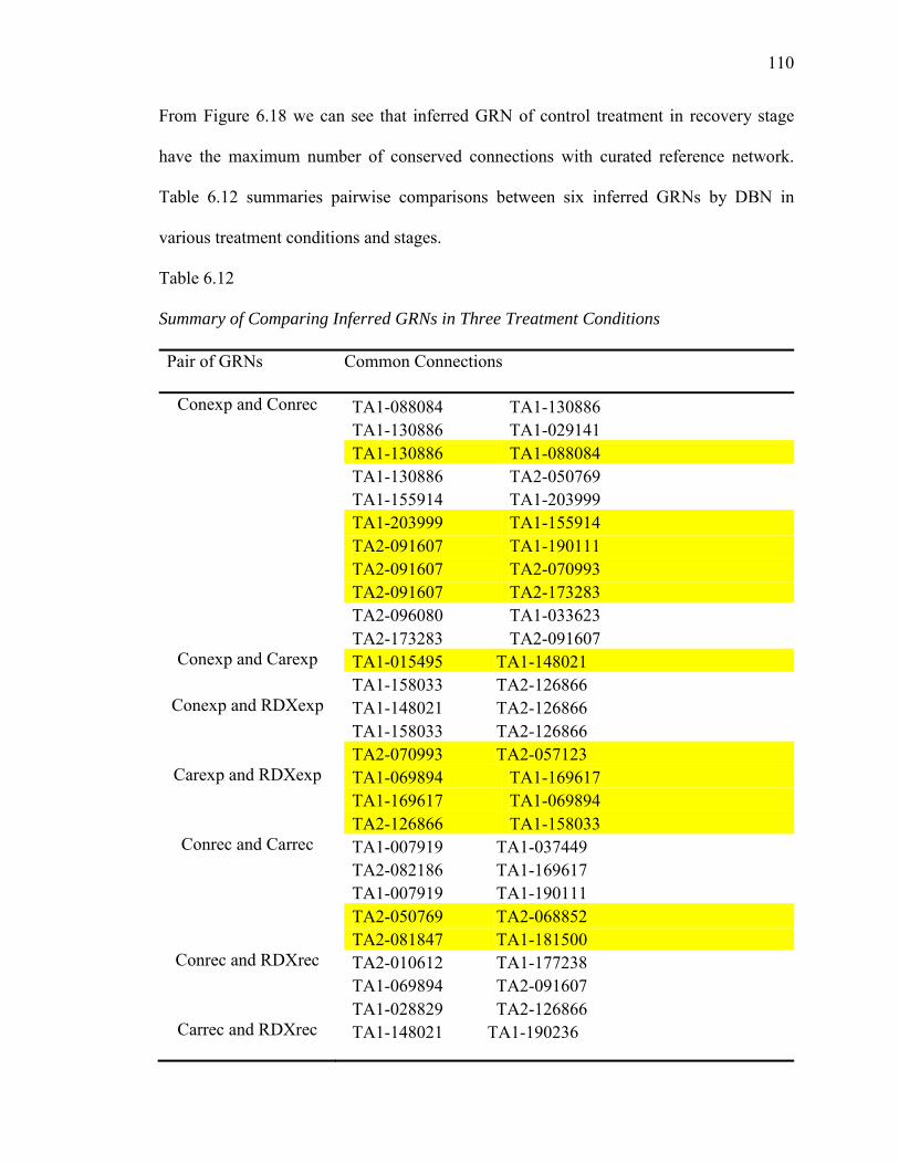
110
From Figure 6.18 we can see that inferred GRN of control treatment in recovery stage
have the maximum number of conserved connections with curated reference network.
Table 6.12 summaries pairwise comparisons between six inferred GRNs by DBN in
various treatment conditions and stages.
Table 6.12
Summary of Comparing Inferred GRNs in Three Treatment Conditions
Pair of GRNs Common Connections
Conexp and Conrec TA1-088084 TA1-130886TA1-130886 TA1-029141TA1-130886 TA1-088084TA1-130886 TA2-050769TA1-155914 TA1-203999TA1-203999 TA1-155914TA2-091607 TA1-190111TA2-091607 TA2-070993TA2-091607 TA2-173283TA2-096080 TA1-033623TA2-173283 TA2-091607
Conexp and Carexp TA1-015495 TA1-148021TA1-158033 TA2-126866
Conexp and RDXexp TA1-148021 TA2-126866TA1-158033 TA2-126866TA2-070993 TA2-057123
Carexp and RDXexp TA1-069894 TA1-169617TA1-169617 TA1-069894TA2-126866 TA1-158033
Conrec and Carrec TA1-007919 TA1-037449TA2-082186 TA1-169617TA1-007919 TA1-190111TA2-050769 TA2-068852TA2-081847 TA1-181500
Conrec and RDXrec TA2-010612 TA1-177238TA1-069894 TA2-091607TA1-028829 TA2-126866
Carrec and RDXrec TA1-148021 TA1-190236

111
Huntington’s Disease
Huntington's disease, chorea, or disorder (HD), is a neurodegenerative genetic
disorder that affects muscle coordination and leads to cognitive decline and dementia. It
typically becomes noticeable in middle age. HD is the most common genetic cause of
abnormal involuntary writhing movements called chorea. The disease is caused by an
autosomal dominant mutation on either of an individual's two copies of a gene called
Huntingtin (Htt gene in KEGG pathway), which means that any child of an affected
parent has a 50% risk of inheriting the disease. The Huntingtin gene normally provides
the genetic information for a protein that is also called “Huntingtin.” The mutation of the
Huntingtin gene codes for a different form of the protein, whose presence results in
gradual damage to specific areas of the brain.
All humans have the Huntingtin gene, which codes for the protein Huntingtin (Htt).
Part of this gene is a repeated section called a trinucleotide repeat, which varies in length
between individuals and may change length between generations. When the length of this
repeated section reaches a certain threshold, it produces an altered form of the protein,
called mutant Huntingtin protein (mHtt). The differing functions of these proteins are the
cause of pathological changes which in turn cause the disease symptoms. The
Huntington's disease mutation is genetically dominant and almost fully penetrant:
mutation of either of a person's HTT genes causes the disease. It is not inherited
according to sex, but the length of the repeated section of the gene, and hence its severity,
can be influenced by the sex of the affected parent [179, 180].
By mapping the 44K earthworm genes to KEGG ortholog genes, a total of 372
transcripts were mapped in the KEGG Huntington's disease pathway and 43 of them are
DEGs from the set of 2574 DEGs. Again, a part of the Huntington’s disease pathway has
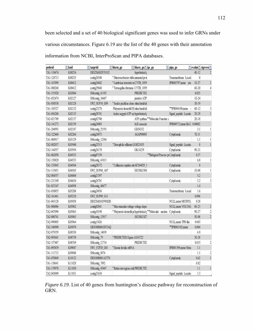
112
been selected and a set of 40 biological significant genes was used to infer GRNs under
various circumstances. Figure 6.19 are the list of the 40 genes with their annotation
information from NCBI, InterProScan and PIPA databases.
Figure 6.19. List of 40 genes from huntington’s disease pathway for reconstruction of GRN.
probeid koid targetid blastn_go blastx_go ips_go pipa_go evalue sigeventTA1-110674 K00234 EB3ZX6E02F5UO2 hypothetical p 4E-12 2TA1-124713 K00235 contig26540 " Dinoroseobacter shibaunnamed prot Transmembrane Locatio 0TA1-167099 K00412 contig24442 " Lumbricus terrestris miCYTB_1059 IPR005797;name ytoc 1E-27 2TA1-080260 K00412 contig29848 " Tetraogallus tibetanus iCYTB_1059 6E-20 4TA1-151920 K02084 SMcontig_61192 PREDICTED 0.025TA1-052474 K02127 SMcontig_36607 putative ATP 1E-24TA1-030538 K02128 EW2_R1P10_E09 " Ixodes pacificus clone mitochondrial 3E-19TA1-185327 K02132 contig23278 Platynereis dumerilii ES mitochondrial """IPR004100;name - 6E-12 3TA1-056208 K02133 contig28741 Aedes aegypti ATP synhypothetical p Signal_peptide Location 2E-29 1TA2-021709 K02137 contig02700 ATP synthase"""Molecular Function: e 2E-18TA2-141273 K02159 contig24085 bcl2-associate IPR000712;name Bcl-2 0.00002TA1-204993 K02187 SMcontig_25193 GD24332 3.1 1TA2-122460 K02266 contig24873 AGAP00085 Cytoplasmic 7E-31TA1-088917 K03129 SMcontig_12304 1.1 1TA2-082037 K03940 contig25313 " Drosoph ila willistoni GGH21035 Signal_peptide Location 0 1TA2-144557 K03954 contig26178 GK14239 Cytoplasmic 9E-21TA1-062050 K04533 contig07159 """Biological Process: pr Cytoplasmic 0.37TA2-158820 K04533 SMcontig_41013 6.8 1TA1-153843 K04564 contig28172 " Callinectes sapidus mitAF264029_1 Cytoplasmic 0TA1-115451 K04565 EW2_R1P04_A07 SJCHGC056 Cytoplasmic 1E-08 1TA2-084557 K04604 contig21397 5.2TA1-231349 K04634 contig26701 Cytoplasmic 5.2 3TA1-023347 K04958 SMcontig_40677 1.4TA1-030855 K05208 contig24936 Transmembrane Locatio 1.6TA2-161461 K05210 EW2_R1P09_G11 0.096TA1-043128 K05858 EB3ZX6E01DWRZB NULL;name METHYL 0.28TA1-006086 K05862 contig02841 " Mus musculus voltage-voltage-depen NULL;name VOLTAG 6E-23 2TA2-047090 K05863 contig10190 " Platynereis dumerilii pahypothetical p"""Molecular unction: Cytoplasmic 9E-27 2TA2-000741 K05863 SMcontig_12917 SJCHGC027 5E-08 2TA2-090805 K05864 contig13426 NULL;name TPR-like 0.043TA2-106990 K05870 EB3O8BM01D3TAQ """IPR003102;name 0.004TA2-079359 K08530 SMcontig_14039 6.9TA2-093641 K08738 SMcontig_79 " PREDICTED: Equus cGJ16722 3E-28TA2-157407 K08769 SMcontig_21734 PREDICTED 0.015 2TA1-093839 K09047 EW1_F2P20_G01 " Eisenia foetida mRNA IPR001396;name Meta 1.1TA1-111713 K09048 SMcontig_8876 1.1 2TA1-070849 K10132 EB3O8BM01A2T70 Cytoplasmic 0.62 1TA1-138641 K11828 SMcontig_7092 0.82TA1-178978 K11830 SMcontig_45447 " Rattus norvegicus coilePREDICTED 1.1 1TA2-045009 K11831 contig23638 Signal_peptide Location 1.3
ttttttt
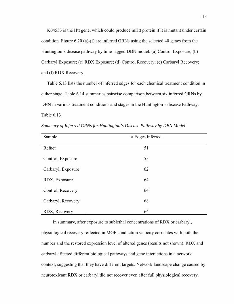
113
K04533 is the Htt gene, which could produce mHtt protein if it is mutant under certain
condition. Figure 6.20 (a)-(f) are inferred GRNs using the selected 40 genes from the
Huntington’s disease pathway by time-lagged DBN model: (a) Control Exposure; (b)
Carbaryl Exposure; (c) RDX Exposure; (d) Control Recovery; (e) Carbaryl Recovery;
and (f) RDX Recovery.
Table 6.13 lists the number of inferred edges for each chemical treatment condition in
either stage. Table 6.14 summaries pairwise comparison between six inferred GRNs by
DBN in various treatment conditions and stages in the Huntington’s disease Pathway.
Table 6.13
Summary of Inferred GRNs for Huntington’s Disease Pathway by DBN Model
Sample # Edges Inferred
Refnet 51
Control, Exposure 55
Carbaryl, Exposure 62
RDX, Exposure 64
Control, Recovery 64
Carbaryl, Recovery 68
RDX, Recovery 64
In summary, after exposure to sublethal concentrations of RDX or carbaryl,
physiological recovery reflected in MGF conduction velocity correlates with both the
number and the restored expression level of altered genes (results not shown). RDX and
carbaryl affected different biological pathways and gene interactions in a network
context, suggesting that they have different targets. Network landscape change caused by
neurotoxicant RDX or carbaryl did not recover even after full physiological recovery.

114
(a)
(b)
Figure 6.20. Inferred GRNs of 40 genes from Huntington’s disease pathway. (a)-(f) are inferred GRNs using the selected 40 genes from Huntington’s disease pathway by time-lagged DBN model: (a) Control Exposure; (b) Carbaryl Exposure; (c) RDX Exposure; (d) Control Recovery; (e) Carbaryl Recovery; and (f) RDX Recovery.
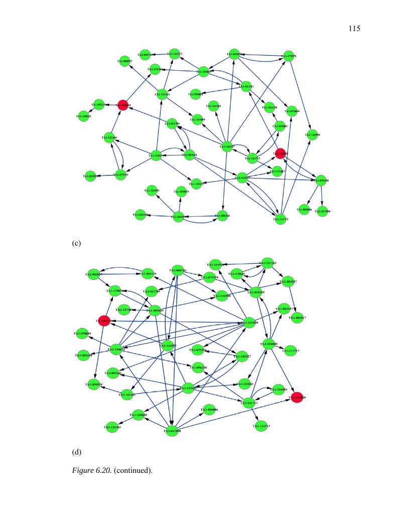
115
(c)
(d)
Figure 6.20. (continued).
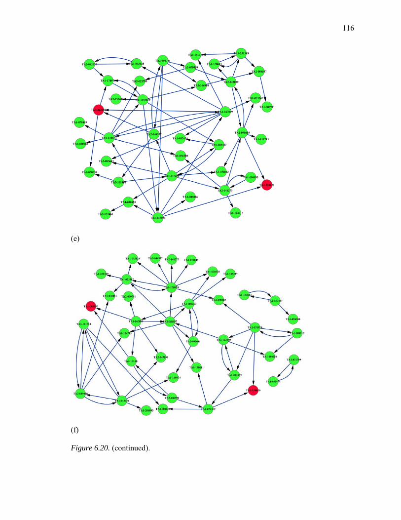
116
(e)
(f)
Figure 6.20. (continued).
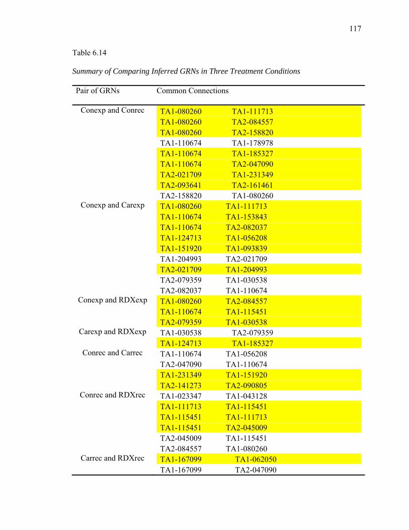
117
Table 6.14
Summary of Comparing Inferred GRNs in Three Treatment Conditions
Pair of GRNs Common Connections
Conexp and Conrec TA1-080260 TA1-111713TA1-080260 TA2-084557TA1-080260 TA2-158820TA1-110674 TA1-178978TA1-110674 TA1-185327TA1-110674 TA2-047090TA2-021709 TA1-231349TA2-093641 TA2-161461TA2-158820 TA1-080260
Conexp and Carexp TA1-080260 TA1-111713TA1-110674 TA1-153843TA1-110674 TA2-082037TA1-124713 TA1-056208TA1-151920 TA1-093839TA1-204993 TA2-021709TA2-021709 TA1-204993TA2-079359 TA1-030538TA2-082037 TA1-110674
Conexp and RDXexp TA1-080260 TA2-084557TA1-110674 TA1-115451TA2-079359 TA1-030538
Carexp and RDXexp TA1-030538 TA2-079359TA1-124713 TA1-185327
Conrec and Carrec TA1-110674 TA1-056208TA2-047090 TA1-110674TA1-231349 TA1-151920TA2-141273 TA2-090805
Conrec and RDXrec TA1-023347 TA1-043128TA1-111713 TA1-115451TA1-115451 TA1-111713TA1-115451 TA2-045009TA2-045009 TA1-115451TA2-084557 TA1-080260
Carrec and RDXrec TA1-167099 TA1-062050TA1-167099 TA2-047090
118
CHAPTER VII
CONCLUSIONS
Summary and Conclusions
Gene Regulatory Networks (GRNs) provide integrated views of gene interactions that
control biological processes. Reconstruction of GRNs from time-series microarray gene
expression data is a very challenging problem for bioinformatics researchers. Although a
number of computational models and algorithms have been developed to infer GRNs,
there is no single outstanding approach that can model GRNs with the best performances
for any given data set. Here, we have developed ISML and RefNet toolboxs that have
shown promising potential in overcoming some of the difficulties in inference of GRNs
and have had some novel biological discovery.
By applying ISML to two microarray datasets, we have identified and optimized small
subsets of classifier/biomarker genes from high dimensional datasets and generated
classification models of acceptable precision for multiple classes.
In the RefNet toolbox, we have developed a cyber-based integrated environment to (1)
build reference GRN/Pathway for non-model organisms; (2) provide biological prior
knowledge of GRN to improve computational models, (3) interpret and compare the
GRNs built from computational models with wet-lab experiments; and (4) serve as a gene
selection tool for GRN reconstruction. This tool was applied to the earthworm Eisenia
fetida, an environmentally important species without a complete genome sequence and
helped identify pathway-related genes from transcriptomic-wide transcripts.
By applying ISML, RefNet and time-lagged DBN to a time-course microarray dataset,
GRNs were inferred for the exposure and the recovery phases of unexposed earthworms
and earthworms exposed to RDX and carbaryl. Differences between these networks are
119
attributed to perturbations caused by chemical exposure. These differences warrant
further biological experiments for validation and validated changes have the great
potential of providing new clues to toxicity targets and modes of action (mechanisms).
Future Directions
There are several areas that we can extend the current work to in the future:
Identification of exposure dose- and duration-specific classifier genes from the
15K earthworm multi-class microarray dataset. Instead of separating the
biological samples into three classes of treatment types, they can be further
classified into six classes: (1) Control day_0 & day_14; (2) Control day_4; (3)
TNT day_0 & day_14; (4) TNT day_4; (5) RDX day_0 & day_14; (6) RDX
day_4. Currently, we are investigating which factor (dose or exposure time) has
more pronounced effects on the gene expression of biological samples.
Many other biological interaction resources and databases may be incorporated in
the RefNet toolbox. To integrate the organism specific reference pathways, genes
and interaction relations in all organism-specific reference pathways will be
merged to form a unified pathways graph. This graph contains the maximum (but,
may be redundant or inaccurate) information extracted from the experimental
validated pathways. The graph will be pruned based on the importance score of
the nodes, which will be computed using a graph ranking algorithm, e.g. page
rank algorithm. Different similarity metrics for comparing pathways can be tested
to generate gene interaction relationships in pathway-pathway relationships for
whole genome of query organism. Furthermore, to validate the pruned pathways,
leave-one-out cross validation can be applied. For the eight model organisms, one
can be used as query, and a pathway based on homologues search against the

120
other seven model organisms can be built. The number of genes and the number
of interaction relations can be used to evaluate the accuracy and the precision of
the proposed method. In addition, we can interpret and display the pathway in
web-based Cytoscape and integrate confirmed prior interaction information to
computational model. Meanwhile, the generated GRN can be used to develop a
gene selection tool to generate a gene set for GRN reconstruction.
Currently, I only used the time-lagged DBN model to reconstruct gene regulatory
networks and only small parts of the constructed reference network by RefNet are
reconstructed. I intend to try other computational approaches such as information
theory based method (e.g., ARACNE), Probabilistic Boolean network model, or
differential equations method to infer gene regulatory network using the same sets
of genes from a specific pathway of interest. Based on the inferred networks from
various methods, their performances such as precision, recall, and run time will be
compared with current inferred results. Furthermore, I also plan to integrate
results of different computational approaches by combining each inferred network
with their performance/scores to generate a more reliable gene regulatory
network. For example, certain connections may exist in the multiple GRNs
inferred using different computational methods, and such connections are
considered more reliable than others inferred by a single method.
121
REFERENCES
[1] Crick, F. (1970): Central Dogma of Molecular Biology. Nature 227, 561-563.
[2] Bodenreider, O. (2004). The unified medical language system (umls): Integrating
biomedical terminology. Nucleic Acids Res, 32 (Database issue):D267–D270.
[3] David P. Clark (2005). Molecular Biology (Understanding the Genetic Revolution),
Chapter 6. Elsevier academic press.
[4] Adomas A, Heller G, Olson A, Osborne J, Karlsson M, Nahalkova J, Van Zyl L,
Sederoff R, Stenlid J, Finlay R, Asiegbu FO (2008). Comparative analysis of transcript
abundance in Pinus sylvestris after challenge with a saprotrophic, pathogenic or
mutualistic fungus. Tree Physiol. 28 (6): 885–897.
[5] Pollack JR, Perou CM, Alizadeh AA, Eisen MB, Pergamenschikov A, Williams CF,
Jeffrey SS, Botstein D, Brown PO (1999). Genome-wide analysis of DNA copy-number
changes using cDNA microarrays. Nat Genet 23 (1): 41–46.
[6] Moran G, Stokes C, Thewes S, Hube B, Coleman DC, Sullivan D (2004).
Comparative genomics using Candida albicans DNA microarrays reveals absence and
divergence of virulence-associated genes in Candida dubliniensis. Microbiology 150 (Pt
10): 3363–3382.
[7] Kulesh DA, Clive DR, Zarlenga DS, Greene JJ (1987). Identification of interferon-
modulated proliferation-related cDNA sequences. Proc Natl Acad Sci USA 84 (23):
8453–8457.
[8] Hacia JG, Fan JB, Ryder O, Jin L, Edgemon K, Ghandour G, Mayer RA, Sun B, Hsie
L, Robbins CM, Brody LC, Wang D, Lander ES, Lipshutz R, Fodor SP, Collins FS
(1999). Determination of ancestral alleles for human single-nucleotide polymorphisms
using high-density oligonucleotide arrays. Nat Genet 22: 164–167.
122
[9] Churchill, GA (2002). Fundamentals of experimental design for cDNA microarrays.
Nature genetics supplement 32: 490.
[10] Patterson, T.A., Lobenhofer, E.K., Fulmer-Smentek, S.B., Collins, P.J., Chu, T.M.,
Bao, W., Fang, H., Kawasaki, E.S., Hager, J., Tikhonova, I.R. et al. Performance
comparison of one-color and two-color platforms within the MicroArray Quality
Control (MAQC) project. Nat Biotechnol, 24(9):1140-1150, 2006.
[11] Shi, L., Reid, L.H., Jones, W.D., Shippy, R., Warrington, J.A., Baker, S.C., Collins,
P.J., de Longueville, F., Kawasaki, E.S., Lee, K.Y. et al. The MicroArray Quality
Control (MAQC) project shows inter- and intraplatform reproducibility of gene
expression measurements. Nat Biotechnol, 24(9):1151-1161, 2006.
[12] Ben-Gal I., Shani A., Gohr A., Grau J., Arviv S., Shmilovici A., Posch S. and Grosse
I. (2005), Identification of Transcription Factor Binding Sites with Variable-order
Bayesian Networks, Bioinformatics, 21(11): 2657-2666.
[13] Yuk Fai Leung and Duccio Cavalieri, Fundamentals of cDNA microarray data
analysis. TRENDS in Genetics 19(11), November 2003
[14] Priness I., Maimon O., Ben-Gal I. (2007), Evaluation of Gene-Expression Clustering
by Mutual Information Distance Measures, BMC Bioinformatics, 8(1):111.
[15] Wei C, Li J, Bumgarner RE. (2004). Sample size for detecting differentially
expressed genes in microarray experiments. BMC Genomics 5 (1): 87.
[16] Emmert-Streib, F. and Dehmer, M. (2008). Analysis of Microarray Data A Network-
Based Approach. Wiley-VCH.
[17] Wouters L, Gõhlmann HW, Bijnens L, Kass SU, Molenberghs G, Lewi PJ (2003).
Graphical exploration of gene expression data: a comparative study of three
multivariate methods. Biometrics 59 (4): 1131–1139.
123
[18] Yang Y, Adelstein SJ, Kassis AI (2009) Target discovery from data mining
approaches. Drug Discov Today 14: 147–154.
[19] Huang LT (2009) An integrated method for cancer classification and rule extraction
from microarray data. J Biomed Sci 16: 25.
[20] Powell WB (2007) Approximate Dynamic Programming: Solving the Curse of
Dimensionality. Hoboken, NJ: Wiley.
[21] Trevino V, Falciani F (2006) GALGO: an R package for multivariate variable
selection using genetic algorithms. Bioinformatics 22: 1154–1156.
[22] Shmulevich I., E.R. Dougherty, K. Seungchan, W. Zhang (2002). Probabilistic
Boolean networks: a rule-based uncertainty model for gene regulatory networks.
Bioinformatics, 18(2): 261–274.
[23] Shmulevich I., Dougherty E. R. and Zhang W (2002). Gene perturbation and
intervention in probabilistic Boolean networks. Bioinformatics, 18 (10):1319-1331.
[24] X. Zhou, X. Wang, and E. R. Dougherty (2003): Construction of genomic networks
using mutual information clustering and reversible-jump Markov-Chain-Monte-Carlo
predictor design. Signal Processing, 83(4), pp. 745--761.
[25] Dougherty, E. R., Kim, S. and Chen, Y (2000). Coefficient of determination in
nonlinear signal processing. Signal Processing, 80:10, pp. 2219-2235. 16.
[26] N. Friedman, K. Murphy, S (1998). Russell: Learning the structure of dynamic
probabilistic networks. Proceedings of the Fourteenth Conference on Uncertainty in
Artificial Intelligence (UAI), 139–147.
[27] J. Yu, V. Smith, P. Wang, A. Hartemink and E Jarvis (2004). Advances to Bayesian
network inference for generating causal networks from observational biological data.
Bioinformatics 20: 3594-603.
124
[28] M. Zou and S. D. Conzen (2005). A new dynamic Bayesian network (DBN)
approach for identifying gene regulatory networks from time course microarray data.
Bioinformatics 21(1): 71-79.
[29] Perrin BE, Ralaivola L et al (2003). Gene networks inference using dynamic
Bayesian networks. Bioinformatics, 19 Suppl 2:II138-II148.
[30] Zhengzheng Xing, Dan Wu (2006): Modeling Multiple Time Units Delayed Gene
Regulatory Network Using Dynamic Bayesian Network. ICDM Workshops, 190-195.
[31] Zhang, L., Samaras, D., Alia-Klein, N., Volkow, N., and Goldstein, R (2006).
Modeling neuronal interactivity using dynamic Bayesian networks. Advances in Neural
Information Processing Systems 18. Eds. Y. Weiss and B. Scholkopf, and J. Platt.
Cambridge, MA: MIT Press.
[32] Li P, Zhang C, Perkins E, Gong P, Deng Y. Comparison of probabilistic boolean
network and dynamic bayesian network approaches for inferring gene regulatory
networks. BMC Bioinformatics. 2007;8(Suppl 7):S13.
[33] Affymetrix: http://www.affymetrix.com/index.affx
[34] Lausted C et al. (2004). POSaM: a fast, flexible, open-source, inkjet oligonucleotide
synthesizer and microarrayer. Genome Biology 5 (8): R58.
[35] Nagaraj SH, Gasser RB, Ranganathan S (Jan 2007). A hitchhiker's guide to
expressed sequence tag (EST) analysis. Brief. Bioinformatics 8 (1): 6–21.
[36] Bammler T, Beyer RP; Consortium, Members of the Toxicogenomics Research;
Kerr, X; Jing, LX; Lapidus, S; Lasarev, DA; Paules, RS; Li, JL et al. (2005).
Standardizing global gene expression analysis between laboratories and across
platforms. Nat Methods 2 (5): 351–356.
125
[37] Pease AC, Solas D, Sullivan EJ, Cronin MT, Holmes CP, Fodor SP. (1994). Light-
generated oligonucleotide arrays for rapid DNA sequence analysis. PNAS 91 (11):
5022–5026.
[38] Nuwaysir EF, Huang W, Albert TJ, Singh J, Nuwaysir K, Pitas A, Richmond T,
Gorski T, Berg JP, Ballin J, McCormick M, Norton J, Pollock T, Sumwalt T, Butcher L,
Porter D, Molla M, Hall C, Blattner F, Sussman MR, Wallace RL, Cerrina F, Green
RD. (2002). Gene expression analysis using oligonucleotide arrays produced by
maskless photolithography. Genome Res 12 (11): 1749–1755.
[39] D. J. Duggan, M. Bittner, Y. Chen, P. Meltzer and J. M. Trent (1999). Expression
profiling using cDNA microarrays. Nature Genetics, 21(1 Suppl.):10–14.
[40] Y. H. Yang, S. Dudoit, P. Luu and T. P. Speed. Normalization for cDNA Microarray
Data. SPIE BiOS 2001, San Jose, California, January 2001.
[41] Yang, Y.H. et al (2002). Normalization for cDNA microarray data: a robust
composite method addressing single and multiple slide systematic variation. Nucleic
Acids Res. 30, e15.
[42] Yang, I.V. et al (2002). Within the fold: assessing differential expression measures
and reproducibility in microarray assays. Genome Biol 3, research0062.1–0062.12.
[43] Cleveland, W.S (1979). Robust locally weighted regression and smoothing
scatterplots. J. Amer. Stat. Assoc. 74, 829–836.
[44] Olga Troyanskaya, Michael Cantor, Gavin Sherlock, Pat Brown, Trevor Hastie,
Robert Tibshirani, David Botstein, and Russ B. Altman, Missing value estimation
methods for DNA microarrays. Bioinformatics (2001) 17(6): 520-525.

126
[45] Alter,O., Brown,P.O. and Botstein,D. (2000) Singular value decomposition for
genome-wide expression data processing and modeling. Proc. Natl Acad. Sci. USA, 97,
10101–10106.
[46] Anderson,T.W. (1984) An Introduction to Multivariate Statistical Analysis. Wiley,
New York.
[47] Golub,G.H. and Van Loan,C.F. (1996) Matrix Computations. Johns Hopkins
University Press, Baltimore, MD.
[48] Eisen, M.B., Spellman, P.T., Brown, P.O (1998). Cluster analysis and display of
genome-wide expression patterns. Proc. Natl Acad. Sci. USA 95, 14863-14868.
[49] Wen, X., Fuhrman, S., Michaels, G.S., Carr, D.B., Smith, S., Barker, J.L. &
Somogy, R (1998). Large-scale temporal gene expression mapping of central nervous
system development. Proc. Natl Acad. Sci. USA 95, 334–339.
[50] Tamayo, P. et al (1999). Interpreting patterns of gene expression with self-
organizing maps: methods and application to hematopoietic differentiation. Proc. Natl
Acad. Sci. USA 96, 2907–2912.
[51] Quackenbush, J (2002). Microarray data normalization and transformation. Nature
Genetics 32, 496-501.
[52] Somorjai R, et al. Class prediction and discovery using gene microarray and
proteomics mass spectroscopy data: curses, caveats, cautions. Bioinformatics
2003;19:1484-1491.
[53] Alon U, et al. Broad patterns of gene expression revealed by clustering analysis of
tumor and normal colon tissues probed by oligonucleotide arrays. Proc. Nat. Acad. Sci.
USA 1999;96:6745-6750
127
[54] Ben-Dor A, et al. Tissue classification with gene expression profiles. J. Comput.
Biol. 2000;7:559-584
[55] Golub T, et al. Molecular classification of cancer: class discovery and class
prediction by gene expression monitoring. Science 1999;286:531-537
[56] Ross D, et al. Systematic variation in gene expression patterns in human cancer cell
lines. Nat. Genet. 2000;24:227-234
[57] Jafari P, Azuaje F. An assessment of recently published gene expression data
analyses: reporting experimental design and statistical factors. BMC Med. Inform.
Decis. Mak. 2006;6:27.
[58] Yvan Saeys, Iñaki Inza, and Pedro Larrañaga, A review of feature selection
techniques in bioinformatics. Bioinformatics (2007) 23(19): 2507-2517.
[59] Dudoit S, et al. Comparison of discriminant methods for the classification of tumors
using gene expression data. J. Am. Stat. Assoc 2002;97:77-87.
[60] Lee J, et al. An extensive comparison of recent classification tools applied to
microarray data. Comput. Stat. and Data Anal. 2005;48:869-885.
[61] Li L, et al. Applications of the GA/KNN method to SELDI proteomics data.
Bioinformatics 2004;20:1638-1640.
[62] Statnikov A, et al. A comprhensive evaluation of multicategory classification
methods for microarray gene expression cancer diagnosis. Bioinformatics 2005;21:631-
643.
[63] Ben-Dor A, et al. Tissue classification with gene expression profiles. J. Comput.
Biol. 2000;7:559-584.
128
[64] Thomas J, et al. An efficient and robust statistical modeling approach to discover
differentially expressed genes using genomic expression profiles. Genome Res.
2001;11:1227-1236.
[65] Newton M, et al. On differential variability of expression ratios: improving statistical
inference about gene expression changes from microarray data. J. Comput. Biol.
2001;8:37-52.
[66] Bø T, Jonassen I. New feature subset selection procedures for classification of
expression profiles. Genome Biol. 2002;3.
[67] Wang Y, et al. Gene selection from microarray data for cancer classification–a
machine learning approach. Comput. Biol. Chem. 2005;29:37-46.
[68] Yeoh E, et al. Classification, subtype discovery, and prediction of outcome in
pediatric lymphoblastic leukemia by gene expression profiling. Cancer Cell
2002;1:133-143.
[69] Gevaert O, et al. Predicting the prognosis of breast cancer by integrating clinical and
microarray data with Bayesian networks. Bioinformatics 2006;22:e184-e190.
[70] Mamitsuka H. Selecting features in microarray classification using ROC curves.
Pattern Recognit. 2006;39:2393-2404.
[71] Xing EP, et al. Feature selection for high-dimensional genomic microarray data.
Proceedings of the Eighteenth International Conference on Machine Learning. 2001.
pp. 601-608.
[72] Blanco R, et al. Gene selection for cancer classification using wrapper approaches.
Int. J. Pattern Recognit. Artif. Intell. 2004;18:1373-1390.
129
[73] Jirapech-Umpai T, Aitken S. Feature selection and classification for microarray data
analysis: evolutionary methods for identifying predictive genes. BMC Bioinformatics
2005;6:148.
[74] Li L, et al. Gene selection for sample classification based on gene expression data:
study of sensitivity to choice of parameters of the GA/KNN method. Bioinformatics
2001;17:1131-1142.
[75] Ooi C, Tan P. Genetic algorithms applied to multi-class prediction for the analysis of
gene expression data. Bioinformatics 2003;19:37-44.
[76] Inza I, et al. Filter versus wrapper gene selection approaches in DNA microarray
domains. Artif. Intell. Med. 2004;31:91-103.
[77] Xiong M, et al. Biomarker identification by feature wrappers. Genome Res.
2001;11:1878-1887.
[78] Segal, E., Shapira, M., Regev, A., Pe'er, D., Botstein, D., Koller, D., and Friedman,
N (2003). Module networks: identifying regulatory modules and their condition-specific
regulators from gene expression data. Nat. Genet. 34, 166-176.
[79] Gardner, T. S., di Bernardo, D., Lorenz, D., and Collins, J. J. (2003). Inferring
genetic networks and identifying compound mode of action via expression profiling.
Science 301, 102-105.
[80] Steuer, R., Kurths, J., Daub, C.O., Weise, J., Selbig, J (2002). The mutual
information: detecting and evaluating dependencies between variables. Bioinformatics
18 (Suppl 2), S231–S240.
[81] Butte, A., Kohane, I (2000). Mutual information relevance networks: Functional
genomics clustering using pairwise entropy measurements. Proceeding of the Pacific
Symposium on Biocomputing, pp. 418–429.
130
[82] Basso, K., Margolin, A.A., Stolovitzky, G., Klein, U., Dalla-Favera (2005). Reverse
engineering of regulatory networks in human B cells. Nat. Genet 37, 382–390.
[83] Opgen-Rhein, R., Strimmer, K (2007). From correlation to causation networks: a
simple approximate learning algorithm and its application to high-dimensional plant
gene expression data. BMC Syst. Biol. 1, 37.
[84] W. Zhao, E. Serpedin, and E. R. Dougherty (2008). Inferring connectivity of genetic
regulatory networks using information-theoretic criteria," IEEE/ACM Transactions on
Computational Biology and Bioinformatics, vol. 5, no. 2, pp.262-274.
[85] Huang S (1999). Gene expression profiling, genetic networks and cellular states: An
integrating concept for tumorigenesis and drug discovery. Journal of Molecular
Medicine, 77:469-480.
[86] Shmulevich I, Gluhovsky I, Hashimoto RF, Dougherty ER, Zhang W (2003).
Steady-state analysis of genetic regulatory networks modeled by probabilistic Boolean
networks. Comparative and Functional Genomics, 4:601-608.
[87] Shmulevich I., Dougherty R., Zhang W (2002). From Boolean to Probabilistic
Boolean Networks as Models of Genetic Regulatory Networks. Proceeding of the IEEE,
90(11), 1778-1792.
[88] H. Lähdesmäki, I. Shmulevich, and O. Yli-Harja (2003). On Learning Gene 52, pp.
147 167.
[89] Voit, E.O (2000). Computational analysis of biochemical systems: a practical guide
for biochemists and molecular biologists. Cambridge University Press, Cambridge, New
York.
[90] De Jong, H (2002). Modeling and simulation of genetic regulatory systems: a
literature review. J. Comput. Biol. 9, 67–103.
131
[91] P. Smolen, D.A. Baxter, and J.H. Byrne (2000). Modeling transcriptional control in
gene networks: Methods, recent results, and future directions. Bulletin of Mathematical
Biology, 62:247_292.
[92] H.D. Landahl (1969). Some conditions for sustained oscillations in biochemical
chaines. Bulletin of Mathematical Biophysics, 31:775_787.
[93] Spieth, C., Hassis, N., Streichert, F (2006). Comparing mathematical models on the
problem of network inference. In: Proceeding of the 8th Annual Conference on Genetic
and evolutionary computation (GECCO 2006),Washington, USA, pp. 279–285.
[94] N. Friedman, et al (2000) Using Bayesian Networks to Analyze Expression Data.
Journal of Computational Biology 7(3-4): 601-620.
[95] N. Dojer, et al (2006). Applying dynamic Bayesian networks to perturbed gene
expression data. BMC Bioinformatics 7(1): 249.
[96] H. Lahdesmki, S. Hautaniemi, I. Shmulevich, O.Yli-Hrja (2006): Relationships
between probabilistic Boolean networks and dynamic Bayesian networks as models of
gene regulatory networks. Signal Processing, volume 86, issue 4, 814 - 834.
[97] Lockhart, D. J. and Winzeler, E. A. (2000). Genomics, gene expression and DNA
arrays. Nature, 405(6788):827–836.
[98] Ankley GT, Daston GP, Degitz SJ, Denslow ND, Hoke RA, et al. (2006)
Toxicogenomics in regulatory ecotoxicology. Environ Sci Technol 40: 4055–4065.
[99] Falciani F, Diab AM, Sabine V, Williams TD, Ortega F, et al. (2008) Hepatic
transcriptomic profiles of European flounder (Platichthys flesus) from field sites and
computational approaches to predict site from stress gene responses following exposure
to model toxicants. Aquat Toxicol 90: 92–101.
132
[100] Nota B, Verweij RA, Molenaar D, Ylstra B, van Straalen NM, et al. (2010) Gene
expression analysis reveals a gene set discriminatory to different metals in soil. Toxicol
Sci 115: 34–40.
[101] Powell WB (2007) Approximate Dynamic Programming: Solving the Curse of
Dimensionality. Hoboken, NJ: Wiley.
[102] Trevino V, Falciani F (2006) GALGO: an R package for multivariate variable
selection using genetic algorithms. Bioinformatics 22: 1154–1156.
[103] Simon R, Lam A, Li MC, Ngan M, Menenzes S, et al. (2007) Analysis of Gene
Expression Data Using BRB-Array Tools. Cancer Inform 3: 11–17.
[104] Horng J, Wu L, Liu B, Kuo J, Kuo W, et al. (2009) An expert system to classify
microarray gene expression data using gene selection by decision tree. Expert Systems
with Applications 36: 9072–9081.
[105] Tan PJ, Dowe DL, Dix TI (2007) Building classification models from microarray
data with tree-based classification algorithms. In: Orgun MA, Thornton J, editors.
Advances in Artificial Intelligence. Berlin, Heidelberg: Springer-Verlag. pp. 589–598.
[106] Abeel T, Helleputte T, Van de PY, Dupont P, Saeys Y (2010) Robust biomarker
identification for cancer diagnosis with ensemble feature selection methods.
Bioinformatics 26: 392–398.
[107] Frank E, Hall M, Trigg L, Holmes G, Witten IH (2004) Data mining in
bioinformatics using Weka. Bioinformatics 20: 2479–2481.
[108] Signal detection theory and ROC analysis in psychology and diagnostics: collected
papers; Swets, 1996.

133
[109] Platt JC (1998) Fast training of support vector machines using sequential minimal
optimization. In: Schoelkopf B, Burges CJC, Smola AJ, editors. Advances in Kernel
Methods: Support Vector Learning. Cambridge, MA: MIT Press. pp. 185–208.
[110] Zhang C, Li P, Rajendran A, Deng Y, Chen D (2006) Parallelization of
multicategory support vector machines (PMC-SVM) for classifying microarray data.
BMC Bioinformatics 7: Suppl 4S15.
[111] Statnikov A, Aliferis CF, Tsamardinos I, Hardin D, Levy S (2005) A
comprehensive evaluation of multicategory classification methods for microarray gene
expression cancer diagnosis. Bioinformatics 21: 631–643.
[112] McLachlan GJ, Chevelu J, Zhu J (2008) Correcting for selection bias via cross-
validation in the classification of microarray data. In: Balakrishnan N, Pena E,
Silvapulle MJ, editors. Beyond Parametrics in Interdisciplinary Research: Festschrift in
Honor of Professor Pranab K. Sen. Institute of Mathematical Statistics. pp. 364–376.
[113] Salwinski L, Miller CS, Smith AJ, Pettit FK, Bowie JU, Eisenberg D. (2004) The
Database of Interacting Proteins: 2004 update. NAR 32:D449-51.
[114] Bader GD, Donaldson I, Wolting C, Ouellette BF, Pawson T, Hogue CW. BIND--
The Biomolecular Interaction Network Database. Nucleic Acids Res. 2001;29(1):242–
245.
[115] Stark C, Breitkreutz BJ, Reguly T, Boucher L, Breitkreutz A, Tyers M. BioGRID: a
general repository for interaction datasets. Nucleic Acids Res. 2006;34(Database
issue):D535–539.
[116] Ceol A, Chatr Aryamontri A, Licata L, Peluso D, Briganti L, Perfetto L, Castagnoli
L, Cesareni G. MINT, the molecular interaction database: 2009 update. Nucleic Acids
Res.2010;38(Database issue):D532–539.

134
[117] Keshava Prasad TS, Goel R, Kandasamy K, Keerthikumar S, Kumar S, Mathivanan
S, Telikicherla D, Raju R, Shafreen B, Venugopal A. et al. Human Protein Reference
Database--2009 update. Nucleic Acids Res. 2009;37(Database issue):D767–772.
[118] Lopes CT, Franz M, Kazi F, Donaldson SL, Morris Q, Bader GD. Cytoscape Web:
an interactive web-based network browser. Bioinformatics. 2010 Jul 23.
[119] Avila-Campillo I, Drew K, Lin J, Reiss DJ, Bonneau R. BioNetBuilder: automatic
integration of biological networks. Bioinformatics. 2007 Feb 1;23(3):392-3. Epub 2006
Nov 30.
[120] Konieczka JH, Drew K, Pine A, Belasco K, Davey S, Yatskievych TA, Bonneau R,
Antin B. BioNetBuilder2.0: bringing systems biology to chicken and other model
organisms. BMC Genomics. 2009 Jul 14;10 Suppl 2:S6.
[121] Xia T, Dickerson JA. OmicsViz: Cytoscape plug-in for visualizing omics data
across species. Bioinformatics. 2008 Nov 1;24(21):2557-8. Epub 2008 Sep 8.
[122] Ferro A, Giugno R, Pigola G, Pulvirenti A, Skripin D, Bader GD, Shasha D.
NetMatch: a Cytoscape plugin for searching biological networks. Bioinformatics. 2007
Apr 1;23(7):910-2.
[123] Kanehisa M, Goto S. KEGG: kyoto encyclopedia of genes and genomes. Nucleic
Acids Res. 2000 Jan 1;28(1):27-30.
[124] Kelley BP, Yuan B, Lewitter F, Sharan R, Stockwell BR, Ideker T. PathBLAST: a
tool for alignment of protein interaction networks. Nucleic Acids Res. 2004 Jul
1;32(Web Server issue):W83-8.
[125] Smith, Temple F.; and Waterman, Michael S. (1981). Identification of Common
Molecular Subsequences. Journal of Molecular Biology 147: 195–197.

135
[126] Lipman, DJ; Pearson, WR (1985). Rapid and sensitive protein similarity
searches. Science 227 (4693): 1435–41.
[127] Pearson, WR; Lipman, DJ (1988). Improved tools for biological sequence
comparison. Proceedings of the National Academy of Sciences of the United States of
America 85 (8): 2444–8. doi:10.1073/pnas.85.8.2444.
[128] Johnson M, Zaretskaya I, Raytselis Y, Merezhuk Y, McGinnis S, Madden TL.
NCBI BLAST: a better web interface. Nucleic Acids Res. 2008;36:W5–W9.
[129] Ye J, McGinnis S, Madden TL. BLAST: improvements for better sequence
analysis. Nucleic Acids Res. 2006;34:W6–W9.
[130] Needleman, Saul B.; and Wunsch, Christian D. (1970). "A general method
applicable to the search for similarities in the amino acid sequence of two proteins".
Journal of Molecular Biology 48 (3): 443–53.
[131] Paul D. Thomas, Michael J. Campbell, Anish Kejariwal, Huaiyu Mi, Brian Karlak,
Robin Daverman, Karen Diemer, Anushya Muruganujan, Apurva Narechania. 2003.
PANTHER: a library of protein families and subfamilies indexed by function. Genome
Res., 13: 2129-2141.
[132] Christian Klukas and Falk Schreiber: Dynamic exploration and editing of KEGG
pathway diagrams. Bioinformatics 2007 23: 344-350.
[133] Hu, Z. Mellor, Snitkin, S. E., & DeLisi, C. (2008). VisANT: an integrative
framework for networks in systems biology, Briefings in Bioinformatics, 2008;9:317-
325.
[134] Hu, Z., et al., (2009) VisANT 3.5: multi-scale network visualization, analysis and
inference based on the gene ontology. 2009 37: W115-W121.
136
[135] P. Holleis, T. Zimmermann, D. Gmach, Drawing Graphs Within Graphs, Journal of
Graph Algorithms and Applications, JGAA, Vol. 9, No. 1, pp. 7-18, 2005.
[136] Opgen-Rhein, R., Strimmer, K (2007). From correlation to causation networks: a
simple approximate learning algorithm and its application to high-dimensional plant
gene expression data. BMC Syst. Biol. 1, 37.
[137] Kauffman SA (1969). Metabolic stability and epigenesis in randomly constructed
genetic nets. Journal of Theoretical Biology, 9:3273-3297.
[138] K. Glass and S. A. Kauffman (1973). The logical analysis of continuous, nonlinear
biochemical control networks. J. Theoret. Biol., vol. 39, pp. 103–129.
[139] S. A. Kauffman (1974): The large scale structure and dynamics of genetic control
circuits: an ensemble approach. J. Theoret. Biol., vol. 44, pp. 167–190.
[140] Kim H, Lee JK, Park T (2007). Boolean networks using the chi-square test for
inferring large-scale gene regulatory networks. BMC Bioinformatics, 8:37.
[141] Antonov AV, Tetko IV, Mader MT, Budczies J, Mewes HW (2004) Optimization
models for cancer classification: extracting gene interaction information from
microarray expression data. Bioinformatics 20: 644–652.
[142] Chi JT, Rodriguez EH, Wang Z, Nuyten DS, Mukherjee S, et al. (2007) Gene
expression programs of human smooth muscle cells: tissue-specific differentiation and
prognostic significance in breast cancers. PLoS Genet 3: 1770–1784.
[143] Choi JK, Yu U, Yoo OJ, Kim S (2005) Differential coexpression analysis using
microarray data and its application to human cancer. Bioinformatics 21: 4348–4355.
[144] Golub TR, Slonim DK, Tamayo P, Huard C, Gaasenbeek M, et al. (1999)
Molecular classification of cancer: class discovery and class prediction by gene
expression monitoring. Science 286: 531–537.
137
[145] Yang Y, Adelstein SJ, Kassis AI (2009) Target discovery from data mining
approaches. Drug Discov Today 14: 147–154.
[146] Huang LT (2009) An integrated method for cancer classification and rule extraction
from microarray data. J Biomed Sci 16: 25.
[147] Gong P, Guan X, Inouye LS, Pirooznia M, Indest KJ, et al. (2007) Toxicogenomic
analysis provides new insights into molecular mechanisms of the sublethal toxicity of
2,4,6-trinitrotoluene in Eisenia fetida. Environ Sci Technol 41: 8195–8202.
[148] Gong P, Guan X, Inouye LS, Deng Y, Pirooznia M, et al. (2008) Transcriptomic
analysis of RDX and TNT interactive sublethal effects in the earthworm Eisenia fetida.
BMC Genomics 9: Suppl 1S15.
[149] Kuperman RG, Simini M, Siciliano SD, Gong P (2009) Effects of energetic
materials on soil organisms. In: Sunahara GI, Lotufo GR, Kuperman RG, Hawari J,
editors. Ecotoxicology of Explosives. Boca Raton, FL: CRC Press. pp. 35–76.
[150] Falciani F, Diab AM, Sabine V, Williams TD, Ortega F, et al. (2008) Hepatic
transcriptomic profiles of European flounder (Platichthys flesus) from field sites and
computational approaches to predict site from stress gene responses following exposure
to model toxicants. Aquat Toxicol 90: 92–101.
[151] Nota B, Verweij RA, Molenaar D, Ylstra B, van Straalen NM, et al. (2010) Gene
expression analysis reveals a gene set discriminatory to different metals in soil. Toxicol
Sci 115: 34–40.
[152] Wang RL, Bencic D, Biales A, Lattier D, Kostich M, et al. (2008) DNA
microarray-based ecotoxicological biomarker discovery in a small fish model species.
Environ Toxicol Chem 27: 664–675.
138
[153] Ankley GT, Daston GP, Degitz SJ, Denslow ND, Hoke RA, et al. (2006)
Toxicogenomics in regulatory ecotoxicology. Environ Sci Technol 40: 4055–4065.
[154] Moens LN, van der V, Van RP, Del-Favero J, De Coen WM (2006) Expression
profiling of endocrine-disrupting compounds using a customized Cyprinus carpio
cDNA microarray. Toxicol Sci 93: 298–310.
[155] Poynton HC, Zuzow R, Loguinov AV, Perkins EJ, Vulpe CD (2008) Gene
expression profiling in Daphnia magna, part II: validation of a copper specific gene
expression signature with effluent from two copper mines in California. Environ Sci
Technol 42: 6257–6263.
[156] Svendsen C, Owen J, Kille P, Wren J, Jonker MJ, et al. (2008) Comparative
transcriptomic responses to chronic cadmium, fluoranthene, and atrazine exposure
in Lumbricus rubellus. Environ Sci Technol 42: 4208–4214.
[157] Gong P, Pirooznia M, Guan X, Perkins EJ (2010) Design, Validation and
Annotation of Transcriptome-Wide Oligonucleotide Probes for the Oligochaete
Annelid Eisenia fetida. PLoS ONE 5(12): e14266.
[158] Edgar R, Domrachev M, Lash AE (2002) Gene Expression Omnibus: NCBI gene
expression and hybridization array data repository. Nucleic Acids Res 30: 207–210.
[159] Yu C, Zavaljevski N, Desai V, Johnson S, Stevens FJ, et al. (2008) The
development of PIPA: an integrated and automated pipeline for genome-wide protein
function annotation. BMC Bioinformatics 9: 52.
[160] Lu Y, Han J (2003) Cancer classification using expression data. Information
Systems 28: 243–268.
[161] Yu L, Liu H (2004) Efficient feature selection via analysis of relevance and
redundancy. Journal of Machine Learning Research 5: 1205–1224.
139
[162] Boutros PC, Okey AB (2005) Unsupervised pattern recognition: an introduction to
the whys and wherefores of clustering microarray data. Brief Bioinform 6: 331–343.
[163] Saeys Y, Inza I, Larranaga P (2007) A review of feature selection techniques in
bioinformatics. Bioinformatics 23: 2507–2517.
[164] Wang Y, Tetko IV, Hall MA, Frank E, Facius A, et al. (2005) Gene selection from
microarray data for cancer classification–a machine learning approach. Comput Biol
Chem 29: 37–46.
[165] Rocke DM, Ideker T, Troyanskaya O, Quackenbush J, Dopazo J (2009) Papers on
normalization, variable selection, classification or clustering of microarray data.
Bioinformatics 25: 701–702.
[166] Jeffery IB, Higgins DG, Culhane AC (2006) Comparison and evaluation of
methods for generating differentially expressed gene lists from microarray data. BMC
Bioinformatics 7: 359.
[167] Anand A, Suganthan PN (2009) Multiclass cancer classification by support vector
machines with class-wise optimized genes and probability estimates. J Theor Biol 259:
533–540.
[168] Hawkins DM (2004) The problem of overfitting. J Chem Inf Comput Sci 44: 1–12.
[169] Suzuki T, Honda M, Matsumoto S, Sturzenbaum SR, Gamou S (2005) Valosine-
containing proteins (VCP) in an annelid: identification of a novel spermatogenesis
related factor. Gene 362: 11–18.
[170] Mosser DD, Caron AW, Bourget L, Meriin AB, Sherman MY, et al. (2000) The
chaperone function of hsp70 is required for protection against stress-induced apoptosis.
Mol Cell Biol 20: 7146–7159.

140
[171] Arcuri F, Papa S, Meini A, Carducci A, Romagnoli R, et al. (2005) The
translationally controlled tumor protein is a novel calcium binding protein of the human
placenta and regulates calcium handling in trophoblast cells. Biol Reprod 73: 745–751.
[172] Southby J, Gooding C, Smith CW (1999) Polypyrimidine tract binding protein
functions as a repressor to regulate alternative splicing of alpha-actinin mutally
exclusive exons. Mol Cell Biol 19: 2699–2711.
[173] Tonevitsky EA, Trushkin EV, Shkurnikov MU, Akimov EB, Sakharov DA (2009)
Changed profile of splicing regulator genes expression in response to exercise. Bull Exp
Biol Med 147: 733–736.
[174] Jorgensen R, Merrill AR, Andersen GR (2006) The life and death of translation
elongation factor 2. Biochem Soc Trans 34: 1–6.
[175] Trabucchi M, Briata P, Garcia-Mayoral M, Haase AD, Filipowicz W, et al. (2009)
The RNA-binding protein KSRP promotes the biogenesis of a subset of microRNAs.
Nature 459: 1010–1014.
[176] Song H, Mugnier P, Das AK, Webb HM, Evans DR, et al. (2000) The crystal
structure of human eukaryotic release factor eRF1–mechanism of stop codon
recognition and peptidyl-tRNA hydrolysis. Cell 100: 311–321.
[177] Gong P, Basu N, Scheuhammer AM, Perkins EJ (2010) Neurochemical and
electrophysiological diagnosis of reversible neurotoxicity in earthworms exposed to
sublethal concentrations of CL-20. Environ Sci Pollut Res Int 17: 181-186.
[178] Orton RJ, Sturm OE, Vyshemirsky V, Calder M, Gilbert DR, Kolch W (Dec 2005).
Computational modelling of the receptor-tyrosine-kinase-activated MAPK pathway.
The Biochemical journal 392 (Pt 2): 249–61.
[179] Walker FO (2007). "Huntington's disease". Lancet 369(9557): 218
141
[180] Kremer B (2002). "Clinical neurology of Huntington's disease". In Bates G, Harper
P, and Jones L. Huntington's Disease – Third Edition. Oxford: Oxford University Press.
pp. 28–53.
[181] Akutsu T, Miyano S, Kuhara S (1999). Identification of genetic networks from a
small number of gene expression patterns under the Boolean network model. Pacific
Symposium on Biocomputing, 4:17-28.
[182] M. Brun, E. R. Dougherty, I. Shmulevich (2005). Steady-State Probabilities for
Attractors in Probabilistic Boolean Networks. Signal Processing, 85, 1993–2013.
[183] Werhli, A.V., Husmeier, D (2007). Reconstructing gene regulatory networks with
Bayesian networks by combining expression data with multiple sources of prior
knowledge. Stat. Appl. Genet. Mol. Biol., 6:Article 15.
[184] Needham, C.J., Bradford, J.R., Bulpitt, A.J.,Westhead, D.R (2007). A primer on
learning in Bayesian networks for computational biology. PLoS Comput. Biol. 3 (8),
e129.
[185] Murphy, K. and Mian, S (1999). Modelling gene expression data using dynamic
Bayesian networks. Technical report, Computer Science Division, University of
California, Berkeley, CA.
[186] Z. Ghahramani (2002). Graphical Models: Parameter Learning. The handbook of
Brain Theory and Neural Networks (2nd edition).
[187] R. Greiner and W. Zhou (2002). Structural extension to logistic regression:
Discriminant parameter learning of belief net classifiers. In AAAI.
[188] H. Wettig, P. Grünwald, T. Roos, P. Myllymäki, and H. Tirri (2003). When
discriminative learning of Bayesian network parameters is easy. In IJCAI2003, pages
491-496.
142
[189] P. Kontkanen, P. Myllymäki, T. Silander, and H. Tirri (1999). On supervised
selection of Bayesian networks. In UAI99, pages 334-342.
[190] A. Ng and M. Jordan (2001). On discriminative versus generative classifiers: A
comparison of logistic regression and naive Bayes. In NIPS.
[191] Murphy, K (2002). Dynamic Bayesian Networks: Representation, Inference and
Learning. PhD dissertation, University of California, Berkeley.
[192] Bayes Net Toolbox. http://www.cs.berkeley.edu/~murphyk/Bayes/bnt.html
[193] S. Liang, S. Fuhrman, et al (1998). Reveal, a general reverse engineering algorithm
for inference of genetic network architectures. Pac Symp Biocomput: 18-29.
[194] Yu,H., Luscombe,N.M., Qian,J. and Gerstein,M (2003). Genomic analysis of gene
expression relationships in transcriptional regulatory networks. Trends Genet, 19, 422–
427.