Microarray Normalization

Xiaole Shirley Liu

STAT115 / STAT215

2

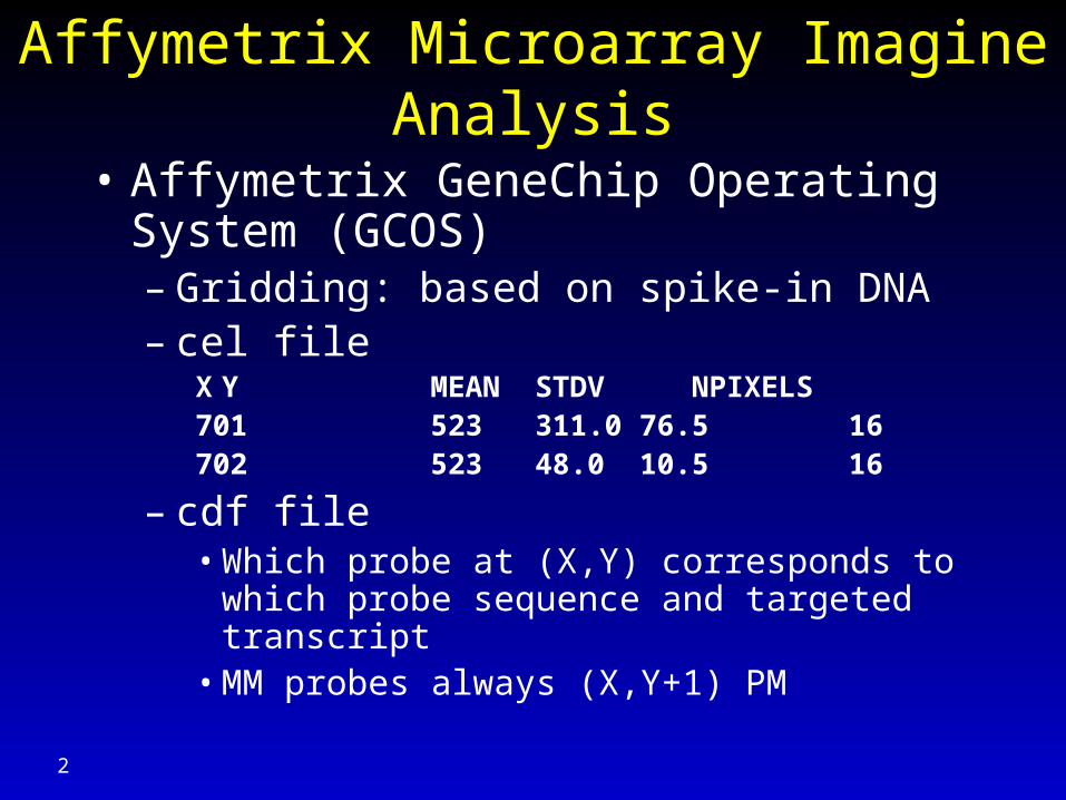
Affymetrix Microarray Imagine Analysis

• Affymetrix GeneChip Operating System (GCOS)– Gridding: based on spike-in DNA– cel file

X Y MEAN STDV NPIXELS

701 523 311.0 76.5 16

702 523 48.0 10.5 16

– cdf file• Which probe at (X,Y) corresponds to which probe

sequence and targeted transcript• MM probes always (X,Y+1) PM

Normalization

• Try to preserve biological variation and minimize experimental variation, so different experiments can be compared

• Assumption: most genes / probes don’t change between two conditions

• Normalization can have larger effect on analysis than downstream steps (e.g. group comparisons)

3

4

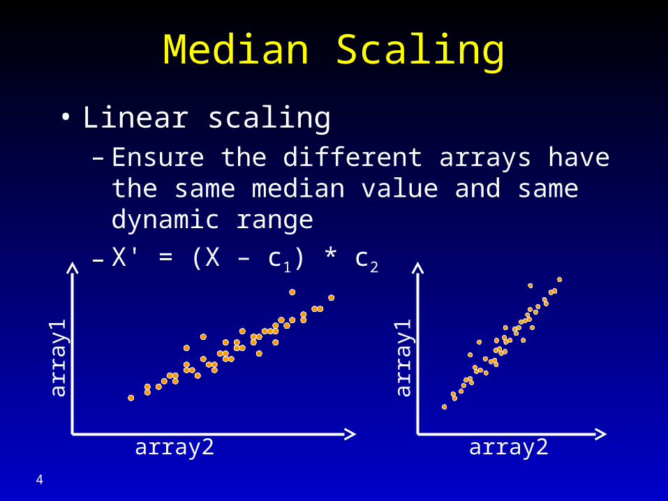
Median Scaling

• Linear scaling– Ensure the different arrays have the same

median value and same dynamic range

– X' = (X – c1) * c2

array2 array2

arra

y1

arra

y1

5

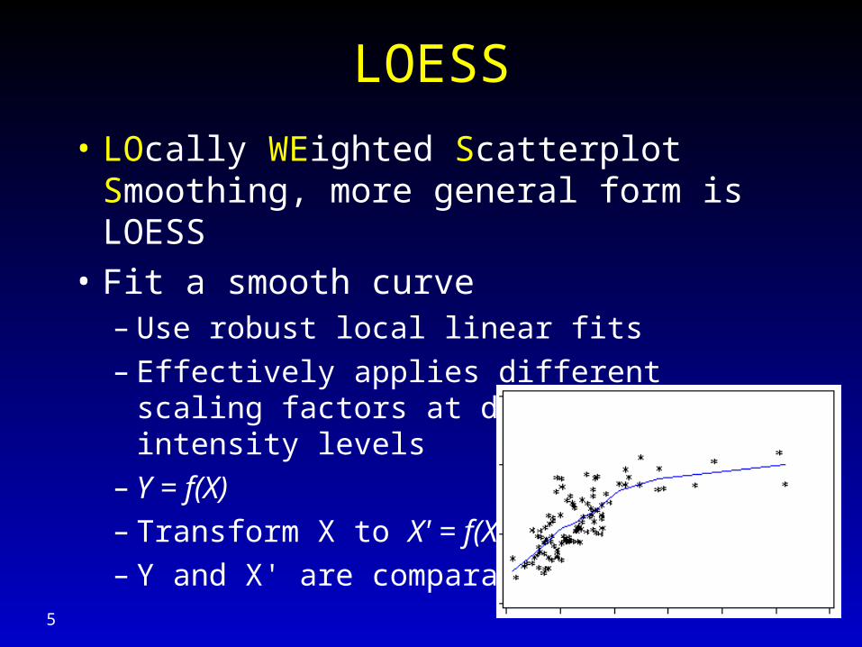
LOESS

• LOcally WEighted Scatterplot Smoothing, more general form is LOESS

• Fit a smooth curve– Use robust local linear fits– Effectively applies different scaling factors at

different intensity levels– Y = f(X)– Transform X to X' = f(X)– Y and X' are comparable

6

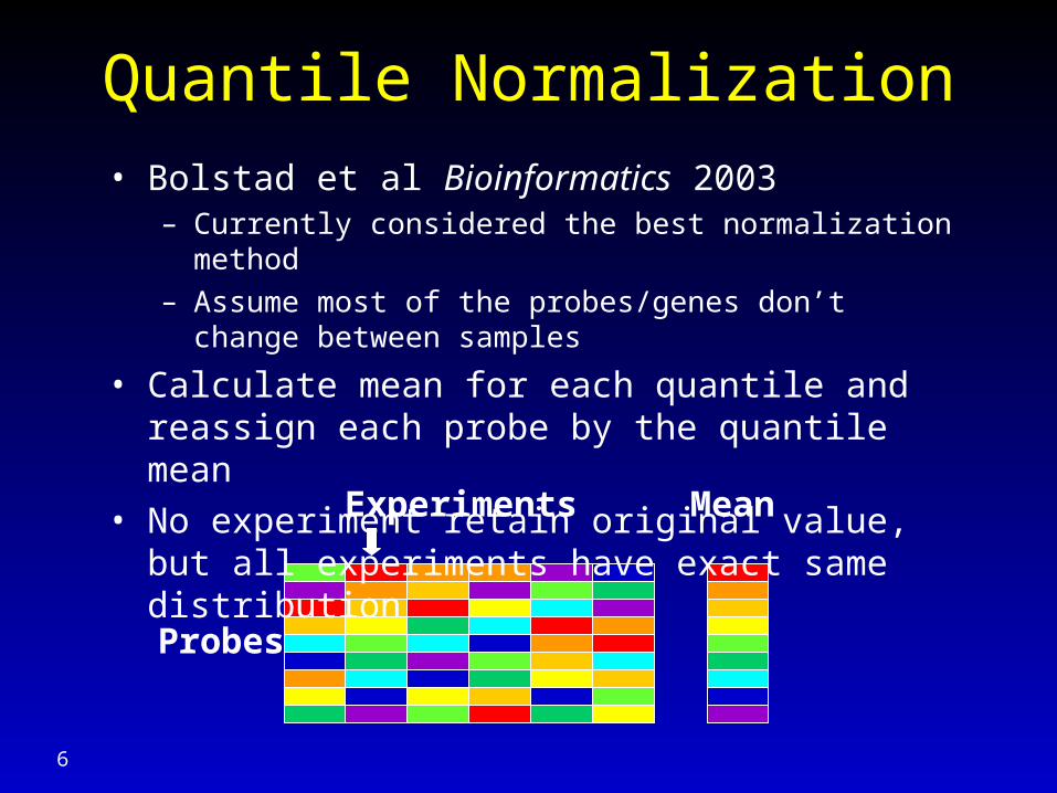
Quantile Normalization

Probes

Experiments Mean

• Bolstad et al Bioinformatics 2003– Currently considered the best normalization method

– Assume most of the probes/genes don’t change between samples

• Calculate mean for each quantile and reassign each probe by the quantile mean

• No experiment retain original value, but all experiments have exact same distribution

How to Visualize Microarray Normalization?

7

8

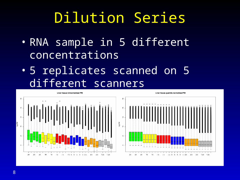
Dilution Series

• RNA sample in 5 different concentrations

• 5 replicates scanned on 5 different scanners

• Before and after quantile normalization

9

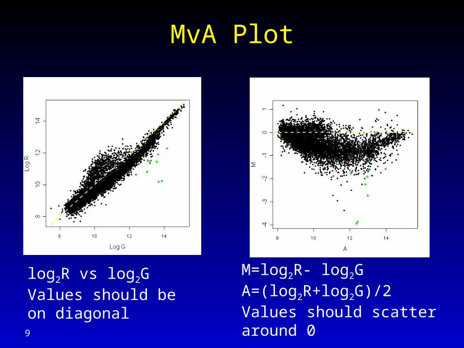
MvA Plot

log2R vs log2G Values should be on diagonal

M=log2R- log2GA=(log2R+log2G)/2Values should scatter around 0

10

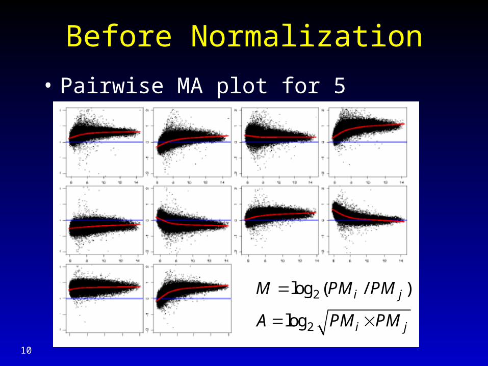
Before Normalization

• Pairwise MA plot for 5 arrays, probe (PM)

2

2

log ( / )

log

i j

i j

M PM PM

A PM PM

11

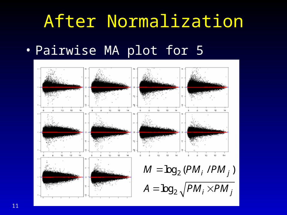
After Normalization

• Pairwise MA plot for 5 arrays, probe (PM)

2

2

log ( / )

log

i j

i j

M PM PM

A PM PM

Gene Expression Index

13

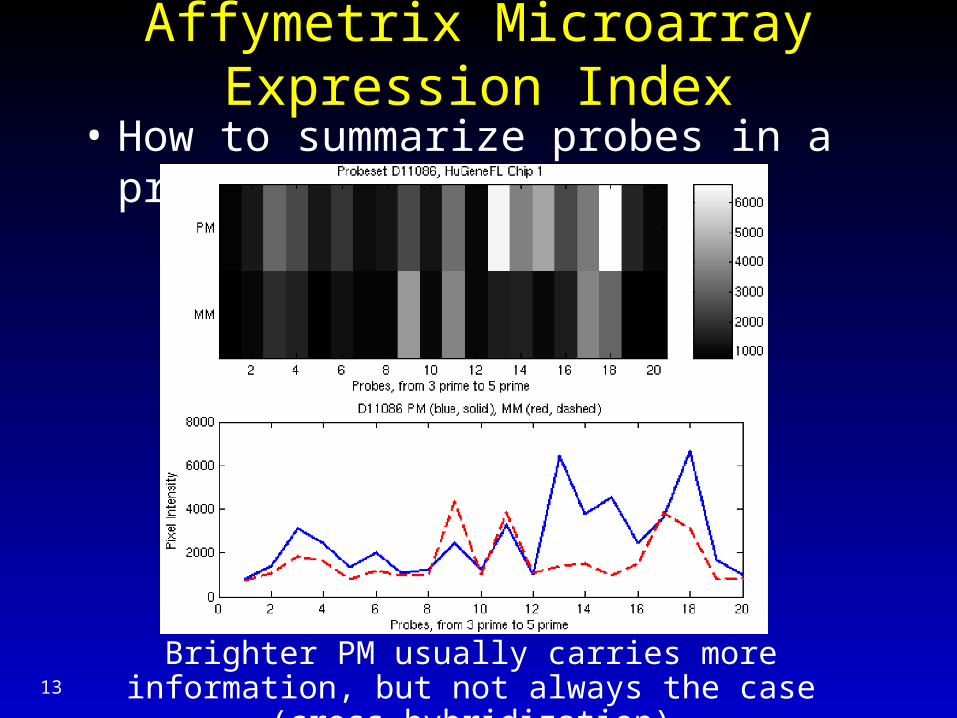
Affymetrix Microarray Expression Index

• How to summarize probes in a probeset?

Brighter PM usually carries more information, but not always the case (cross-hybridization)

14

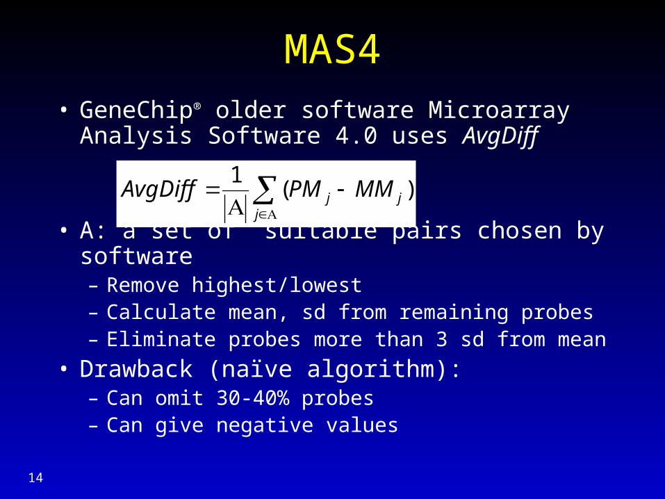
MAS4• GeneChip® older software Microarray Analysis

Software 4.0 uses AvgDiff

• A: a set of suitable pairs chosen by software– Remove highest/lowest– Calculate mean, sd from remaining probes– Eliminate probes more than 3 sd from mean

• Drawback (naïve algorithm):– Can omit 30-40% probes – Can give negative values

j

jj MMPMAvgDiff )(1

15

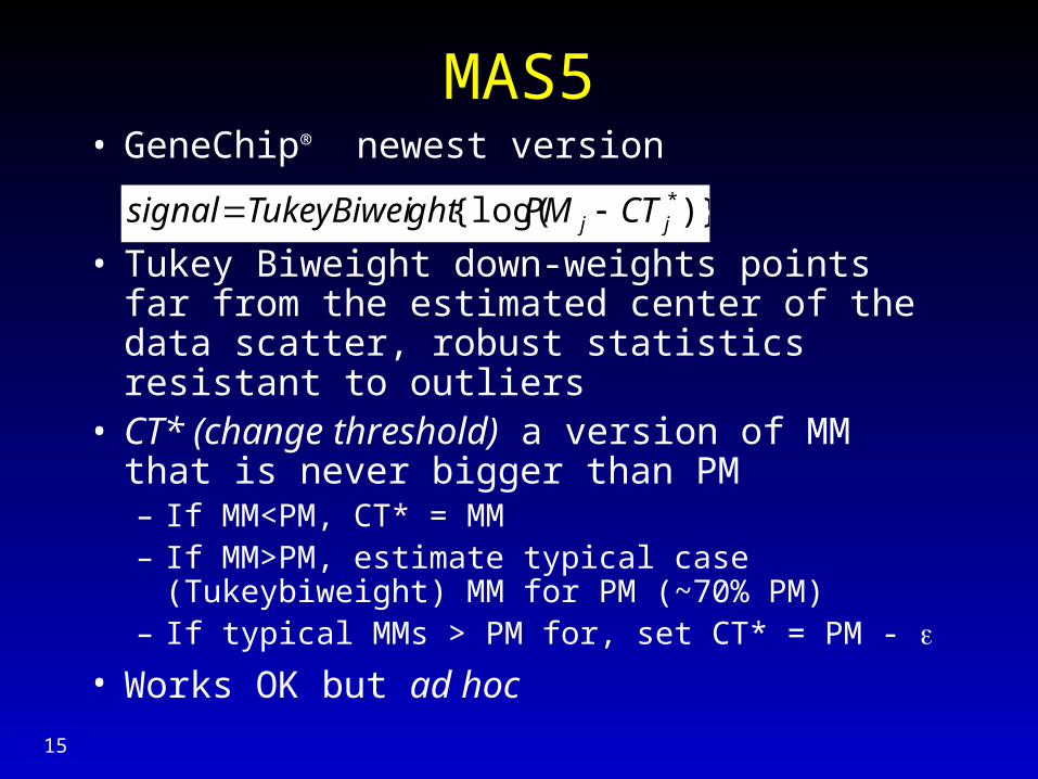
MAS5• GeneChip® newest version

• Tukey Biweight down-weights points far from the estimated center of the data scatter, robust statistics resistant to outliers

• CT* (change threshold) a version of MM that is never bigger than PM– If MM<PM, CT* = MM– If MM>PM, estimate typical case (Tukeybiweight)

MM for PM (~70% PM)– If typical MMs > PM for, set CT* = PM -

• Works OK but ad hoc

)}{log( *jj CTPMghtTukeyBiweisignal

16

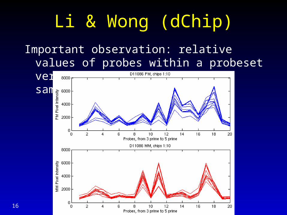
Li & Wong (dChip)

Important observation: relative values of probes within a probeset very stable across multiple samples.

17

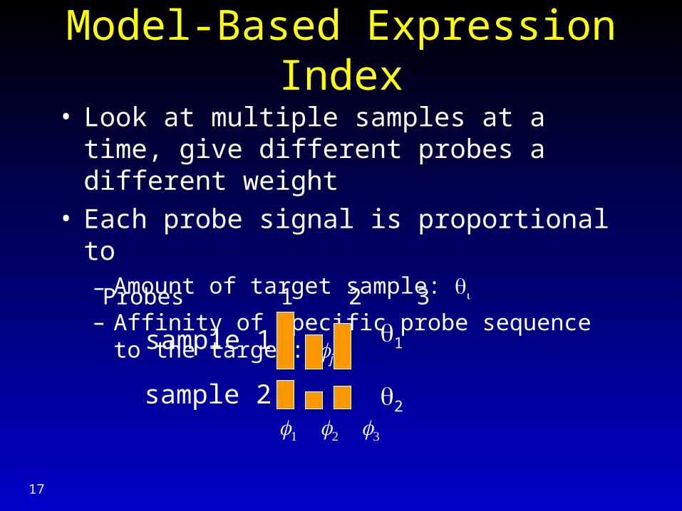
Model-Based Expression Index

• Look at multiple samples at a time, give different probes a different weight

• Each probe signal is proportional to – Amount of target sample:

– Affinity of specific probe sequence to the target: j

1

2

Probes 1 2 3

sample 1

sample 2

18

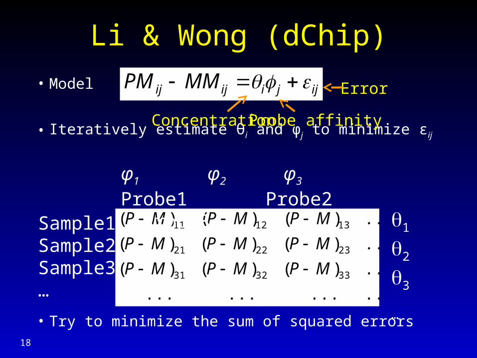
Li & Wong (dChip)

• Model

• Iteratively estimate θi and φj to minimize εij

• Try to minimize the sum of squared errors

ijjiijij MMPM

............

...)()()(

...)()()(

...)()()(

333231

232221

131211

MPMPMP

MPMPMP

MPMPMP

Sample1

Sample2Sample3…

φ1 φ2 φ3

Probe1 Probe2 Probe3 …1

2

3

…

Concentration Probe affinity

Error

19

RMA = Robust Multi-chip Analysis

• Irizarry & Speed, 2003

• 1: Probe intensity background adjustment

• 2: Quantile normalize the Log transformed background adjusted PM

• 3: Robust probe summary

20

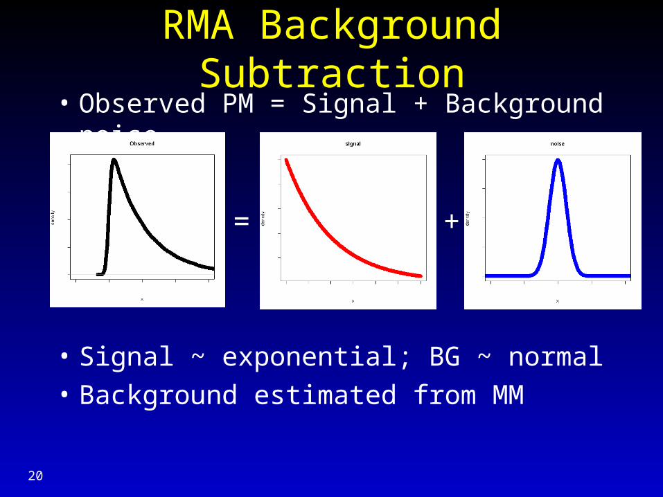
RMA Background Subtraction• Observed PM = Signal + Background noise

• Signal ~ exponential; BG ~ normal

• Background estimated from MM

+=

21

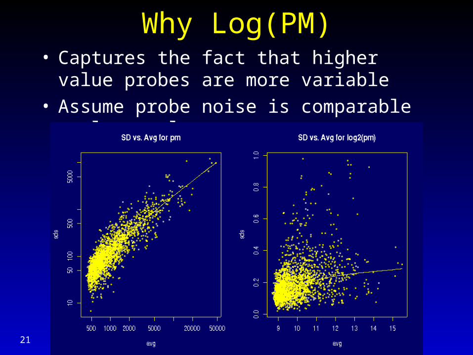
Why Log(PM)• Captures the fact that higher value probes are

more variable• Assume probe noise is comparable on log scale

22

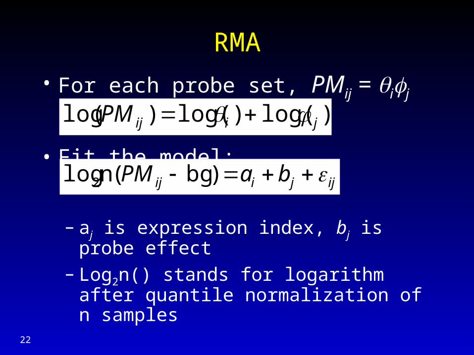
• For each probe set, PMij = ij

• Fit the model:

– aj is expression index, bj is probe effect– Log2n() stands for logarithm after quantile

normalization of n samples

RMA

)log()log()(log jiijPM

ijjiij baPM )bg(nlog2

RMA

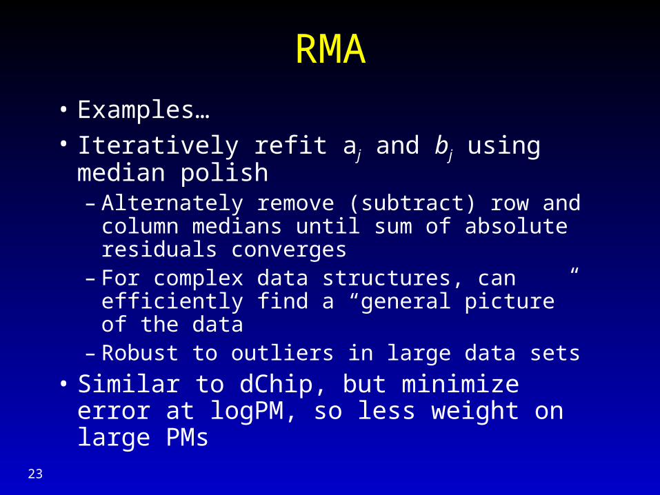
• Examples…• Iteratively refit aj and bj using median

polish– Alternately remove (subtract) row and column

medians until sum of absolute residuals converges

– For complex data structures, can efficiently find a “general picture” of the data

– Robust to outliers in large data sets

• Similar to dChip, but minimize error at logPM, so less weight on large PMs

23

Gene Expression IndexMethod Comparison

25

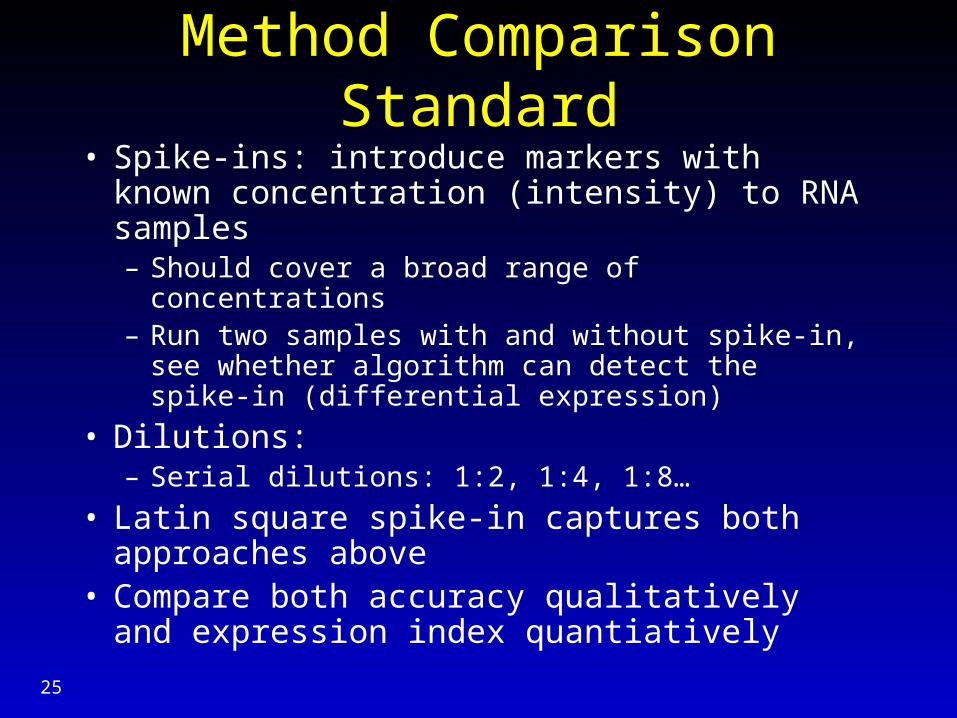
Method Comparison Standard• Spike-ins: introduce markers with known

concentration (intensity) to RNA samples– Should cover a broad range of concentrations– Run two samples with and without spike-in, see

whether algorithm can detect the spike-in (differential expression)

• Dilutions: – Serial dilutions: 1:2, 1:4, 1:8…

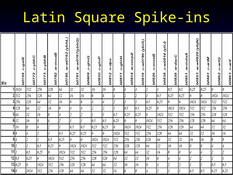
• Latin square spike-in captures both approaches above

• Compare both accuracy qualitatively and expression index quantiatively

26

Latin Square Spike-ins

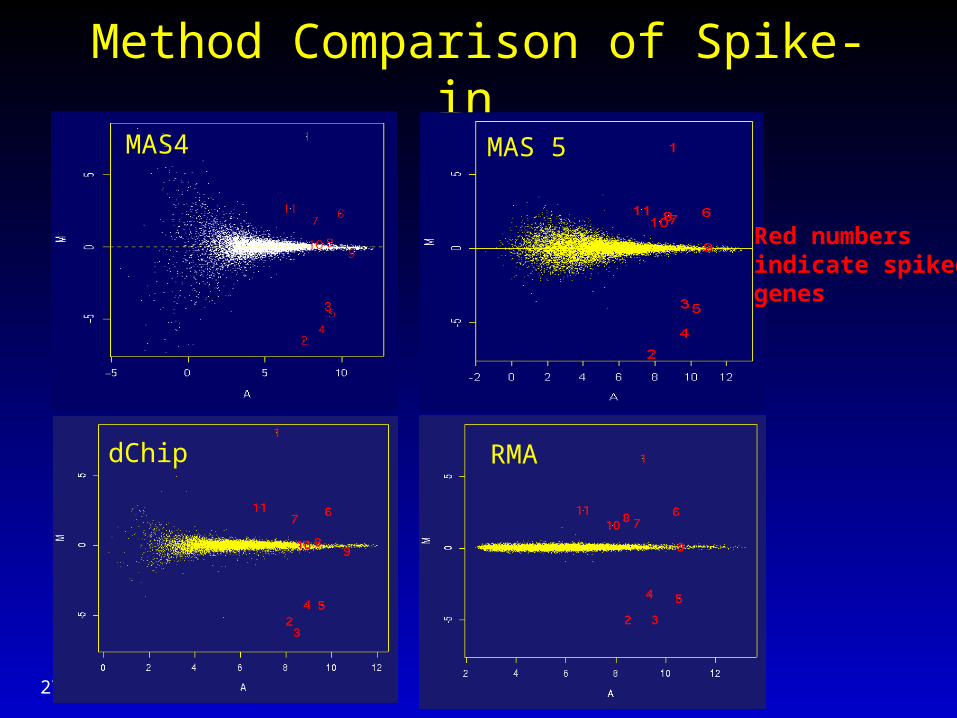
Method Comparison of Spike-in

27

MAS4 MAS 5

dChip RMA

Red numbers indicate spikedgenes

Summary

• Cel file and cdf file. • Array normalization: Loess, qnorm

– Assumptions

• Normalization visualization: MA plots• Gene Expression Index

– RMA models probe effect in expression arrays

– Use MM to correct background

– Qnorm log (PM)

– Median polish, model probe behavior to get expression index

• Method comparison28