MICROECONOMICS

TOPIC 3

Economics 2013-14

SUPPLY

NATURE OF PRODUCTION

SPECIALISATION

Modern production is based on the principle of specialisation.

Specialisation is using a resource in the productive capacity for which it is best suited.

Helps to use scarce resources efficiently.

BENEFITS OF SPECIALISATION

Increases the amount produced

Reduces the cost per unit produced

Efficient use of scarce resources.

APPLYING SPECIALISATION

Can be seen a number of different levels:

National – countries specialising eg coffee Regional – different areas of one country eg

farming Industry eg whisky Firm eg whisky distilling, bottling Worker – called DIVISION OF LABOUR

DIVISION OF LABOUR

ADVANTAGES FOR THE WORKER

Increased productivity leading to increased income

More skills acquired

Gain more job satisfaction

DISADVANTAGES FOR THE WORKER

Increased risk of unemployment – too specialised and can’t do anything else

Interdependence of workers

Monotony of tasks – gets boring!!!

PRODUCTION DECISIONS

Producers want to maximise their profits.

One way to do this is to use the most efficient method of production in order to keep cost per unit low.

In the short run, the capacity of the firm is fixed and so the firm will only be able to produce a maximum number of products

In the long run, the capacity of the firm can be increased or decreased, which can change the level of production.

PRODUCTION IN THE SHORT RUN:LAW OF DIMINISHING RETURNS

Factors of production – land, labour, capital and enterprise.

Returns are what a producer gets back in output when they employ more of a variable factor of production.

Example – returns to labour means the output gained when more labour is employed.

In the short run when deciding what output will be the most efficient to produce the firm must take into consideration the LAW OF DIMINISHING RETURNS

This states that as a producer uses more of a factor of production the returns to begin with will increase but diminishing returns will eventually happen.

TYPES OF OUTPUT

Total Output – the total amount produced

Marginal Output – the extra output produced when an extra factor of production is employed

Average Output – the average amount produced. Normally TOTAL OUTPUT divided by NUMBER OF WORKERS

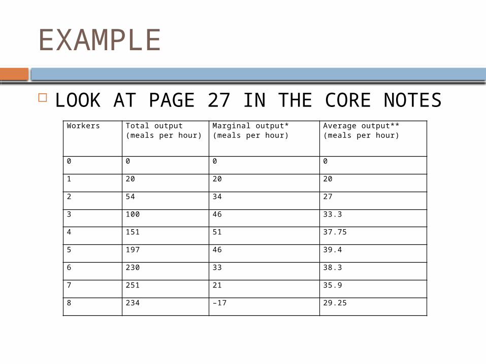
EXAMPLE

LOOK AT PAGE 27 IN THE CORE NOTESWorkers Total output

(meals per hour)Marginal output*(meals per hour)

Average output**(meals per hour)

0 0 0 0

1 20 20 20

2 54 34 27

3 100 46 33.3

4 151 51 37.75

5 197 46 39.4

6 230 33 38.3

7 251 21 35.9

8 234 –17 29.25

Increasing Marginal Returns – occurs when marginal output is growing.

Diminishing Marginal Returns – occurs when marginal output is decreasing.

PRODUCTION IN THE LONG RUN in the long run all factors of production

are variable.

The firm can change its capacity which is also called changing the scale of its operations.

RETURNS TO SCALE

Increasing Returns to Scale – output grows faster than the size of the firm. Also called ECONOMIES OF SCALE

Constant Returns to Scale – output rises at the same rate as the size of the firm.

Decreasing Returns to Scale – output rises slower than the size of the firm – also called DISECONOMIES OF SCALE

Economies of Scale

The advantages of large scale production that result in lower unit (average) costs (cost per unit)

AC = TC / Q Economies of Scale – spreads total costs

over a greater range of output

ECONOMIES OF SCALE

Often referred to as the ADVANTAGES OF BEING A BIG COMPANY

Two types:

Internal – improvements in output (productivity) as the firm grows in size

External – improvements in output which a firm gains from growth of its industry.

INTERNAL ECONOMIES OF SCALE Technical Financial Purchasing Managerial

Marketing Research and

development (R&D)

Risk bearing Welfare

INTERNAL ECONOMIES OF SCALE

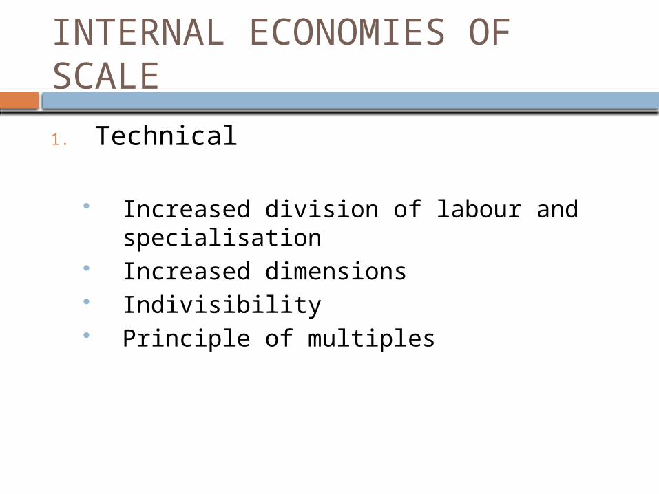
1. Technical

Increased division of labour and specialisation

Increased dimensions Indivisibility Principle of multiples

2. Financial

Easier to attract investors due to low risk

Borrow money at lower rates of interest

3. Purchasing

Gain large discounts for buying in bulk

Dictate to suppliers price, quality and delivery date they want

4. Managerial

Can afford to employ specialist staff e.g. an accountant

5. Marketing

Costs can be spread over a larger volume of sales

Transport costs per unit are lowered as ships, lorries etc are full.

6. Research and Development

Can afford to research

Can gain a competitive advantage through innovation

Maintain market share through product development

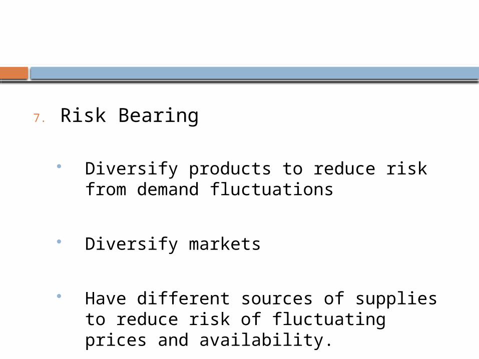
7. Risk Bearing

Diversify products to reduce risk from demand fluctuations

Diversify markets

Have different sources of supplies to reduce risk of fluctuating prices and availability.

8. Welfare

Can afford to offer benefits to employees that will increase motivation and efficiency.

Pensions Medical services Fringe benefits Recreational facilities

Economies of Scale

Capital Land Labour Output TC AC

Scale A 5 3 4 100

Scale B 10 6 8 300

Assume each unit of capital = £5, Land = £8 and Labour = £2Calculate TC and then AC for the two different ‘scales’ (‘sizes’) of production facilityWhat happens and why?

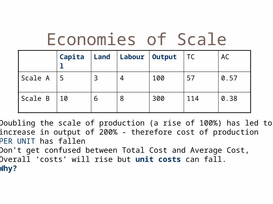
Economies of ScaleCapital Land Labour Output TC AC

Scale A 5 3 4 100 57 0.57

Scale B 10 6 8 300 114 0.38

Doubling the scale of production (a rise of 100%) has led to an increase in output of 200% - therefore cost of production PER UNIT has fallenDon’t get confused between Total Cost and Average Cost, Overall ‘costs’ will rise but unit costs can fall.Why?

EXTERNAL ECONOMIES OF SCALE Normally happens when firms in an

industry are focused in a particular area.

They can gain the following advantages:

Lower training costs Ancillary services provided by specialist

suppliers Co-operation of firms

DISECONOMIES OF SCALE

These are the disadvantages of being a big company.

INTERNAL DISECONOMIES

Management problems – difficult to control

Waste is difficult to control or detect.

EXTERNAL DISECONOMIES

Shortages of skilled labour and high wages

Shortage of raw materials

Congestion and high transport costs

COSTS OF PRODUCTION

These are the money values of resources used in producing a good or service.

Wages to labour Rent for land Interest on capital

The owner of the firm provides enterprise. If revenue earned is equal to cost of production this is called NORMAL PROFIT, if revenue is greater than costs, it is called SUPERNORMAL PROFITS

TYPES OF COSTS

Fixed Costs

Costs which do not change with output.

If nothing is made fixed costs still need to be paid

Examples include rent and insurance.

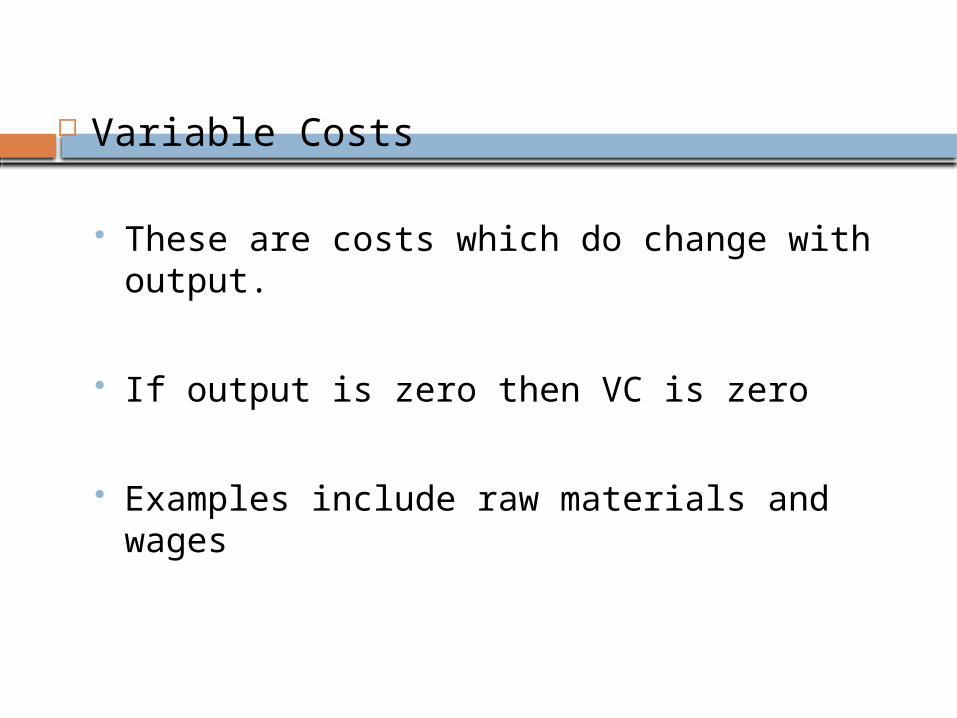
Variable Costs

These are costs which do change with output.

If output is zero then VC is zero

Examples include raw materials and wages

Total Costs

This is fixed costs plus variable costs

Average (Total) Cost

Total Costs divided by Output

Can also be called UNIT COST

Average Fixed Cost

Fixed cost divided by Output

Average Variable Cost

Variable cost divided by Output

Marginal Cost

The extra cost of producing one additional unit of output.

E.g. The MC of the 50th unit is the Total Cost of the 50th unit minus the Total Cost of the 49th Unit.

MC = TC n – TCn-1

SHORT RUN AND LONG RUN

In the short run the firm will have fixed capacity.

Some costs will be fixed and some variable

In the long run all costs are variable.

SHORT RUN COSTS

LOOK AT TABLE ON PAGE 35 OF CORE NOTES

DRAW THE GRAPHS

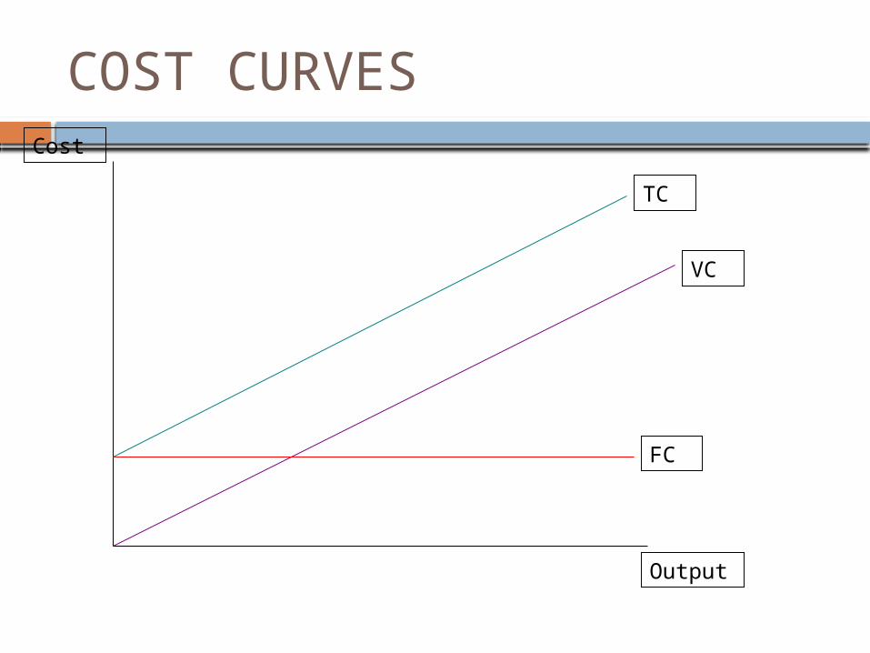
COST CURVES

Output

Cost

FC

TC

VC

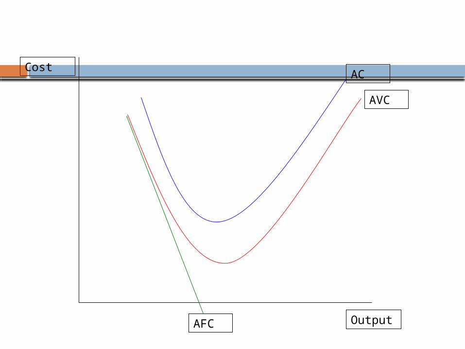
Output

Cost

AFC

AVC

AC

Output

CostACMC

AVC

OBSERVATIONS

When output increases in the short run:

Fixed costs do not change

Variable costs increase, not always at a constant rate

Total costs increase at the same rate as variable costs

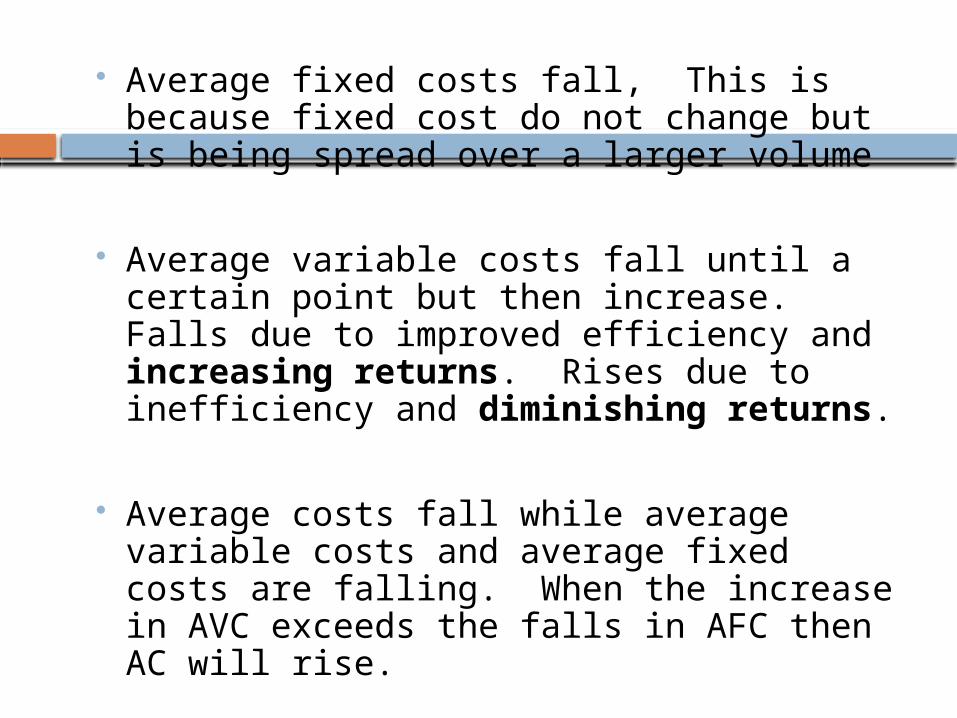
Average fixed costs fall, This is because fixed cost do not change but is being spread over a larger volume

Average variable costs fall until a certain point but then increase. Falls due to improved efficiency and increasing returns. Rises due to inefficiency and diminishing returns.

Average costs fall while average variable costs and average fixed costs are falling. When the increase in AVC exceeds the falls in AFC then AC will rise.

Combining the Factors of Production

In the short run a firm cannot change its fixed factors of production (eg land) but it can change its variable factors (eg labour)

Law of Diminishing Returns

As successive units of one factor are added to fixed amounts of other factors the increments in total output at first rise and then decline.

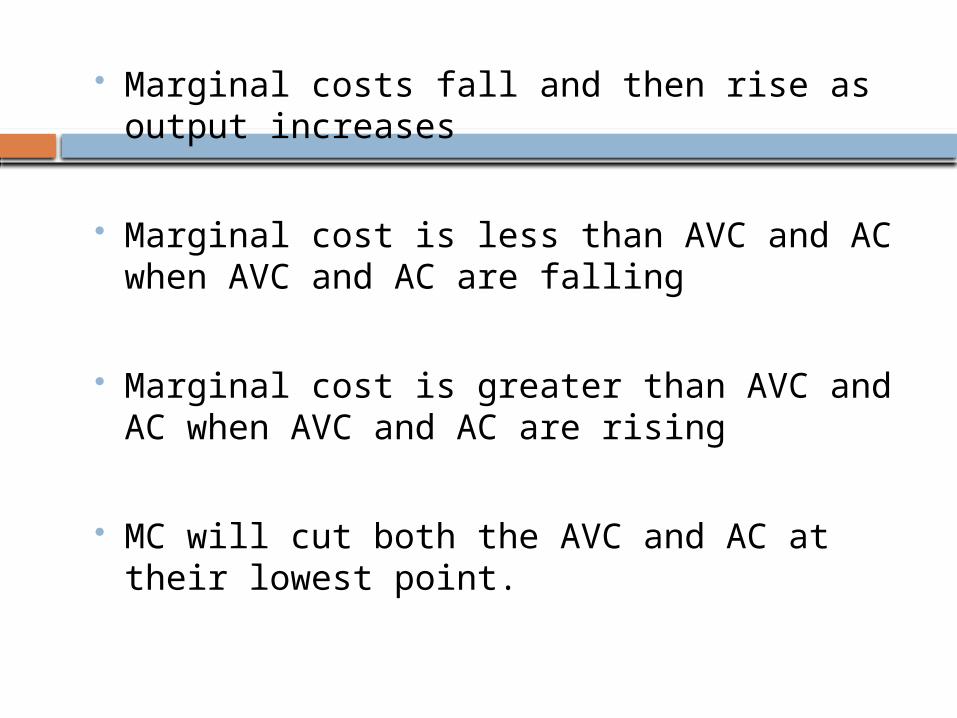
Marginal costs fall and then rise as output increases

Marginal cost is less than AVC and AC when AVC and AC are falling

Marginal cost is greater than AVC and AC when AVC and AC are rising

MC will cut both the AVC and AC at their lowest point.

OPTIMUM OUTPUT

This is the output where the firm would be technically efficient.

At this point AC is at its lowest.

DIMINISHING RETURNS AND COSTS IN THE SHORT RUN

When a firm has increasing marginal returns it will have falling marginal costs

Diminishing marginal returns means rising marginal costs

Increasing average returns means falling average cost

Diminishing average returns means rising average cost

OUTPUT DECISION IN THE SHORT RUN

Firms want to maximise profits.

Any decision on how much to produce is based on the relationship between their sales revenue and their costs.

REVENUE

Total Revenue – total amount earned from selling output;

quantity sold X price per unit

Average Revenue – total revenue divided output. If only one product is sold then AR will be the same as price.

Marginal Revenue is the extra revenue from selling an extra unit of output.

MC = TR n – TRn-1

When a firm sells all its output at the same price, price and MR will be the same.

PROFIT MAXIMISING

This can be determined in two ways.

1. Maximum profit is where the difference between total revenue and total cost is greatest.

2. Where MC = MR

SHUT DOWN POSITION IN THE SHORT RUN

As long as a firm’s TR covers VC then the firm will stay open.

Any money left over from paying VC can be used to pay towards TC and reduce the loss the firm will make.

Shut down would be where TR is less than VC or when price is less than AVC

In the long run the firm must make at least normal profit.

COSTS IN THE LONG RUN

In the long run all costs and factors of production are variable.

Average cost in the long run fall because of economies of scale and rise due to diseconomies of scale.

The AC curve in the long run is U-shaped and has a series of interlinking Short Run AC curves.

The point where LRAC is at its lowest is the optimum size of the firm.

REMEMBER!!!

Short Run Average Costs fall due to increasing average returns to the variable factor

They rise due to diminishing average returns to the variable factor

Short Run Marginal Costs fall due to increasing marginal returns to the variable factor

They rise due to diminishing marginal returns to the variable factor

In the long run Average Costs falls due to economies of scale and rises due to diseconomies of scale.

SUPPLYUNIT 1

TOPIC 3

DEFINITION

Supply is the quantity of a good or service that firms are able and willing to supply at a certain price.

Individual supply is the supply of one firm

Market supply is the supply of all firms in the market.

EFFECT OF PRICE ON SUPPLY

As the price of a product increases the supply of that product will rise.

Represented by a MOVEMENT along the supply curve.

This is due to:-

Existing producers will to supply more to earn more profit

New firms entering the market to earn higher profits

SUPPLY CURVE

Qty

PriceS

S

Supply Curve for Product A

P

P1

Q Q1

CONDITIONS OF SUPPLY

A condition of supply will cause the supply curve to either:

shift to the left (a decrease in supply)

or

shift to the right (an increase in supply)

Prices of other commodities

Competitive Supply – where a supplier will switch resources from the production of one product to another as a result of an increase in price.

Example – price of beef increases so there would be a shift to the right of the beef supply curve.

Joint Supply – a rise in the price could lead to an increase in supply of another commodity

Example – increase in price of petrol leads to the increase in supply of other oil products e.g. bitumen.

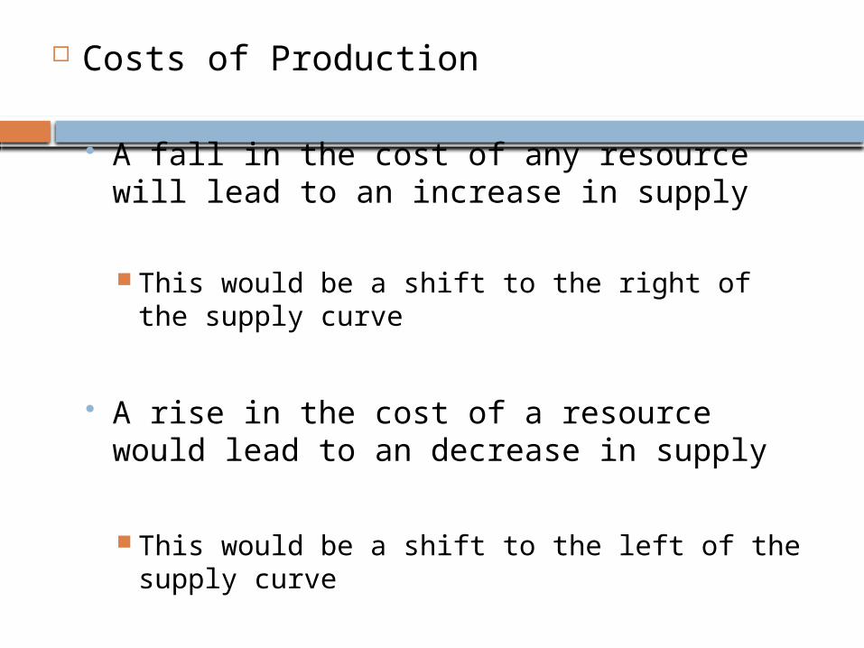
Costs of Production

A fall in the cost of any resource will lead to an increase in supply

This would be a shift to the right of the supply curve

A rise in the cost of a resource would lead to an decrease in supply

This would be a shift to the left of the supply curve

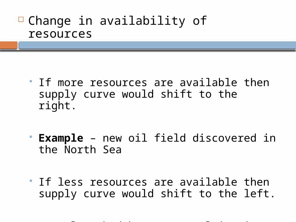
Change in availability of resources

If more resources are available then supply curve would shift to the right.

Example – new oil field discovered in the North Sea

If less resources are available then supply curve would shift to the left.

Example – bad harvest resulting in less wheat

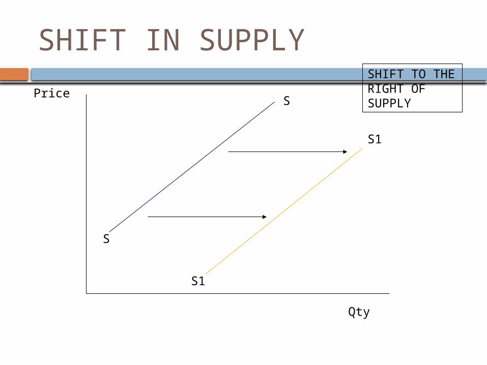
SHIFT IN SUPPLY

Qty

Price

SHIFT TO THE RIGHT OF SUPPLY

S

S

S1

S1

ELASTICITY OF SUPPLYUNIT 1

TOPIC 3

DEFINTION

Price elasticity of supply measures the responsiveness of supply to a change in price.

How do suppliers react when there is a change in the price of their product?

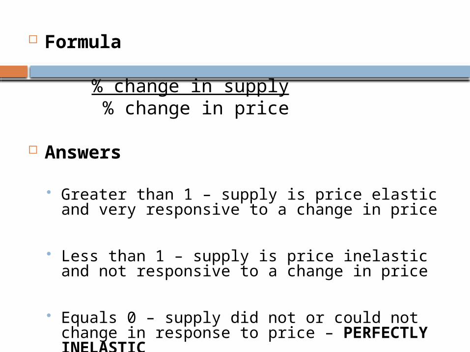
Formula

% change in supply % change in price

Answers

Greater than 1 – supply is price elastic and very responsive to a change in price

Less than 1 – supply is price inelastic and not responsive to a change in price

Equals 0 – supply did not or could not change in response to price – PERFECTLY INELASTIC

FACTOR AFFECTING ELASTICITY OF SUPPLY The only factor that affects supply is TIME

In the short run a firm that is at full capacity cannot change its supply in response to a change in price.

Supply would be perfectly inelastic and the supply curve would be a vertical straight line.

PERFECTLY INELASTIC SUPPLY CURVE

Qty

Price S

If the firm has spare capacity and stocks then it will be able to increase supply

The more spare capacity or more stock the firm has then the more elastic supply will be.

A LITTLE SPARE CAPACITY SOME SPARE STOCKS

PLENTY SPARE CAPACITY, PLENTY STOCKS

Qty Qty

PricePrice

In the long run, supply will be elastic.

Firms will have time to increase their capacity and new firms can enter the market.