ECONOMIC GROWTH CENTERYALE UNIVERSITY

P.O. Box 208629New Haven, CT 06520-8269

http://www.econ.yale.edu/~egcenter/

CENTER DISCUSSION PAPER NO. 936

Microfinance GamesXavier GinéWorld Bank

Pamela JakielaUniversity of California, Berkeley

Dean KarlanYale University

Jonathan MorduchNew York University

June 2006

Notes: Center Discussion Papers are preliminary materials circulated to stimulate discussions andcritical comments.

We thank Shachar Kariv, Edward Miguel, Chris Udry, and participants in the University ofGroningen 2005 conference on microfinance, NEUDC 2005, and seminars at Yale and UCBerkeley. Antoni Codinas, Gissele Gajate, Jacob Goldston, Marcos Gonzales, and KarenLyons provided excellent research assistance in the field. We thank the World Bank, SocialScience Research Council Program in Applied Economics, the UC Berkeley Institute forBusiness and Economic Research, and Princeton University for funding.

This paper can be downloaded without charge from the Social Science Research Networkelectronic library at: http://ssrn.com/abstract=912301

An index to papers in the Economic Growth Center Discussion Paper Series is located at:http://www.econ.yale.edu/~egcenter/research.htm

Microfinance Games

Xavier GinéPamela JakielaDean Karlan

Jonathan Morduch

Abstract

Microfinance has been heralded as an effective way to address imperfections in credit markets. From

a theoretical perspective, however, the success of microfinance contracts has puzzling elements. In

particular, the group-based mechanisms often employed are vulnerable to free-riding and collusion,

although they can also reduce moral hazard and improve selection. We created an experimental

economics laboratory in a large urban market in Lima, Peru and over seven months conducted

eleven different games that allow us to unpack microfinance mechanisms in a systematic way. We

find that risk-taking broadly conforms to predicted patterns, but that behavior is safer than optimal.

The results help to explain why pioneering microfinance institutions have been moving away from

group-based contracts.

JEL Codes: O12, D92, D10, D21, D82, C93

Keywords: microfinance, group lending, information asymmetries, contract theory, experimental economics

2

1 Introduction Banking in low-income communities is a notoriously difficult business. Banks typically

have limited information about their customers and often find it costly or impossible to

enforce loan contracts. Customers, for their part, frequently lack adequate collateral or

credit histories with commercial banks. Moral hazard and adverse selection, coupled with

small transaction sizes, together limit the possibilities for banks to lend profitably.

Despite these obstacles, over the past three decades microfinance practitioners

have defied predictions by finding workable mechanisms through which to make small,

uncollateralized loans to poor customers. Repayment rates on their unsecured loans often

exceed 95 percent, and by 2005 (officially-designated by the United Nations as the

“International Year of Microcredit”), microfinance institutions had served about 100

million customers around the world.

This achievement has been exciting to many, and advocates describe

microfinance as a revolutionary way to reduce poverty (Yunus 1999). From a theoretical

perspective, though, the success has puzzling elements. Many of the new mechanisms

rely on groups of borrowers to jointly monitor and enforce contracts themselves.

However, group-based mechanisms tend to be vulnerable to free-riding and collusion.

Inefficiencies are well known to emerge in similar contexts: examples are documented in

the literatures on public goods, the tragedy of the commons, insurance, and

environmental externalities (Gruber (2005), e.g., describes examples).

We created an experimental economics laboratory in a large, urban market in

Lima, Peru, and conducted eleven different games which allow us to unpack

microfinance mechanisms in a systematic way.1 The experiments took place twice a week

for seven months. All of the participants were small-scale entrepreneurs in the market. By

design, the demographic and economic profiles of participants are similar to those of

1 Harrison and List (2004) would classify the approach as a series of “framed field experiments.” Examples of the approach in other settings include List (2004) and Barr and Kinsey (2002). The closest study to this paper is Cassar, Crowley and Wydick (2005) which conducts a series of repeated public goods games, framed as a decision to repay a loan, in South Africa and Armenia in order to relate contributions to likely behavior in a microfinance setting.

3

microfinance customers in urban Peru. The simulated microfinance transactions involved

players choosing hypothetical risky investments, receiving loans, and managing the risk

of default. In a typical day, we played two or three games, and over seven months of

experimental sessions each of the eleven variants of the game was played on average 27

times. Participants were compensated based on their success as investors in the

simulations. By working in Lima and designing the games to replicate actual

microfinance scenarios, our aim has been to understand the logic of the mechanisms with

individuals likely to participate in an actual microfinance program, but not to replicate

exactly customers’ experience with microfinance.

The simulated environment allowed us to test systematically many of the features

embedded in lending contracts; such a strategy would be impractical for bankers. By

playing a sequence of games with the same individuals, we are able to isolate the impact

of contract from innate propensities to take risks. Second, the experiment allows us to

control the nature of risky choices thus allowing us to gauge explicitly impacts on risk-

taking.

We show that the tendency toward free-riding also emerges in experimental

settings that simulate microfinance transactions: moral hazard is exacerbated by simple

group-based microfinance contracts. However, we show that moral hazard is allayed by

allowing customers to form their own groups voluntarily. Moreover, the mutual insurance

induced by joint liability can allow borrowers to invest in profitable risky projects

without reducing overall repayment rates. Given endogenous group formation,

microfinance contracts do function effectively to reduce moral hazard and facilitate

profitable risk-taking. We find that in the most “true-to-life” game, participants tend, in

fact, to take too little risk relative to the optimum. The finding is consistent with a strong

role for social factors in group settings.

We find in particular that participants who have a propensity to take risks tend to

reduce their risk-taking when their partners act more safely. The result is consistent with

4

altruism or fairness, rather than profit maximization.2

In Section 2, we discuss the microfinance mechanisms that motivate the

experiments. In Section 3, we outline the competing roles of ex ante moral hazard and

mutual insurance that are at the heart of the study. Section 4 describes the lab setting and

participant pool. Section 5 presents theoretical predictions and initial data that relate

contract structure to individual choices. Section 6 presents our main empirical results, and

Section 7 concludes.

2 Microfinance mechanisms Microfinance loan contracts typically include multiple and overlapping mechanisms

aimed at reducing the risk of default. A large theoretical literature details how these

components work in isolation to mitigate problems arising from information

asymmetries, but empirical progress in sorting out the pieces has proved slower.

To see the complexity, consider the following microfinance mechanism, often

called a “group lending” or “joint liability” contract; it is based on models first employed

in South Asia and Latin America in the late 1970s. The mechanism begins with a lender

deciding to enter a new location. In preparation for entry, the lender announces to

residents of the community that in order to access credit, potential customers must first

form small groups. In Bangladesh, groups have typically been restricted to five people,

but sizes vary across programs and regions. Borrowers obtain loans and invest the funds

independently, selecting investments based on the technologies available and their own

perceptions of risk and return. Access to loans continues without interruption as long as

all loans are repaid. But all group members are denied future credit if any member fails to

repay. In this sense, the group members are jointly liable for the loan repayments of their

peers.

This way, group liability is used to harness customers’ information about each

other and their mutual relationships to the lender’s advantage. First, group self-formation

2 For instance, see Rabin (1993) and Fehr and Schmidt (1999) for recent work that incorporates fairness into decision-making models.

5

provides a screening mechanism that can help to reduce adverse selection (e.g., Ghatak

1999). In addition, moral hazard can be reduced either by fostering cooperation among

group members (e.g., Stiglitz 1990) or through repeated interactions (Armendariz de

Aghion and Morduch 2000). The group element provides an inducement for members to

monitor each other (Banerjee, Besley and Guinnane 1994) and to punish each other in the

face of moral hazard, possibly through social sanctions (Wydick 1999; Karlan 2005a). In

sum, group liability can potentially reduce risk-taking and improve the lender’s

repayment rate. It could also increase risk-taking, though, by fostering a mutual insurance

arrangement within the group. This could be helpful for the bank and customers

(Sadoulet 2000), could lead to free-riding, or to collusion against the bank (Besley and

Coate 1995). By just observing the mechanism as implemented, it is difficult to

determine the relative importance of group formation, dynamic incentives, monitoring,

enforcement, insurance, free-riding, or collusion.

Ideally, researchers would like to analyze the behavior of customers who are

(randomly) offered a wide range of different credit contracts, each designed to reveal the

logic behind a particular component. As a practical matter, though, this kind of

randomized variation is difficult to implement. Identifying the role of each component,

though, is critical for understanding how microfinance markets function – and for

determining where the largest payoff to innovation might lie. We use the methods of

experimental economics to understand the logic of existing microfinance mechanisms

and illuminate various theoretical explanations of their performance. The experimental

setting also allows us to accommodate psychological and social forces that may

systematically operate alongside standard economic motivations.

3 Risky investments The games were designed to capture the logic of the best-known microfinance contract

features, focusing on moral hazard and the ways that contracts reduce default rates by

enabling partners to insure one another and by creating social costs to individual default.

To disentangle the relative importance of specific mechanisms behind joint liability

6

contracts, we place participants in an experimental setting inspired by Stiglitz’s (1990)

model of ex ante moral hazard in microfinance. We then extend the model to consider the

impact of introducing opportunities for monitoring, coordination, and enforcement.

Note that ex-ante moral hazard broadly construed includes many types of

behavior. The typical description involves entrepreneurs changing from a safe project to a

risky project due to incentives from the loan contract. For a microentrepeneur who

manages a small shop, such a change could be subtle, e.g., buying more inventory than

they would normally, or buying a new product for which the revenue is uncertain. Ex-

ante moral hazard might also be manifested in diversion of the loan from business to

household needs, hence lowering expected revenue. Although microfinance lenders

typically target micro-entrepreneurs, it is widely accepted that many borrowers use the

proceeds for consumption smoothing (Menon 2003; Armendariz de Aghion and Morduch

2005). Our benchmark game extends Stiglitz’s model of moral hazard to a dynamic

framework where agents make repeated project choice decisions. Each participant was

first given a game sheet marked with spaces for ten rounds, but participants were told that

the game might end after any given round and we varied the ending round across games.

In the analysis below, we focus on the first six rounds only to minimize potential survivor

biases (participants with a propensity to choose the safe project will be disproportionately

represented among active participants as the game proceeds); the qualitative results are

robust to restricting analyses to even earlier rounds.

In each round, participants were given a “loan” of 100 points and instructed to

invest it in one of two projects: a safe project (“project square”) which yielded a return of

200 points with certainty or a riskier project (“project triangle”) that pays out 600 points

with probability ½ and zero otherwise. At no time during the games did we refer to the

choices as “safe” and “risky.”

An individual whose project succeeded had to repay her loan, while an individual

whose project failed did not; wealth from prior rounds could not be used to repay the

current round’s loan. Thus limited liability – and hence the possibility of moral hazard –

7

is introduced. In each round, the safe project had an expected (and certain) net return of

100 points after repaying the principal, whereas the risky project had an expected return

of 250 points (50 percent chance of 500 points and 50 percent chance of zero).

In Stiglitz’s model, as in much of the theoretical work on microfinance, safer

projects are assumed to have higher expected returns than riskier projects, and,

consequently, the bank's optimum is equivalent to the social optimum. In that context, an

optimal contract induces a safe project choice. We relax this assumption here for several

reasons. First, our pilot games suggested that participants were risk averse even over

small stakes. When gross project returns were equal in expectation, risk aversion

appeared to eliminate moral hazard, and most participants chose the project that was

optimal from the bank’s perspective. In light of this finding, we calibrated the project

returns so that approximately equal numbers of participants would choose the safe and

the risky project in the benchmark games. In our most “true-to-life” game, the calibration

yields an average loan repayment rate (94 percent) that approximates repayment rates

achieved by leading microfinance institutions.

The second rationale for the payoff structure is that the assumption that risky

projects have higher expected returns than safe projects is more realistic than the

alternative assumption that the expected returns to safe projects are higher (de Meza and

Webb 1990). One objective in expanding financial access is to enable borrowers to make

risky investments in pursuit of higher incomes – and the structure highlights this

possibility.

We compare individual liability games to outcomes under a “joint liability” (JL)

contract structure that captures elements of the “group lending” approach described in the

previous section. In the joint liability treatments, each participant was matched with a

single partner3 and investment payouts depend on both one’s own decisions and one’s

partner’s choices. Table 1 shows the expected net returns. If both partners choose safe

investments, their outcomes are identical to those in the benchmark individual game:

each participant is guaranteed a safe return of 100 points. But if a safe investor is 3 We test different matching processes, including random and anonymous, random and public, as well as peer-selected.

8

partnered with someone who chooses the risky investment, the safe investor can expect to

bail out its partner half the time. The only case in which the group may not be able to

repay the bank occurs when both partners choose risky investments and fail, a situation

that occurs with a probability of one quarter chance given that outcomes are independent.

From the risk-taker’s point of view, choosing the risky investment when the

partner chooses the safe investment is a particularly winning arrangement – though it

imposes burdens on the partner. From the lender’s perspective, risk-taking may result in

lower repayment rates. In this sense, risk taking has an element of moral hazard.

However, note that the payoff structure is such that some degree of risk-taking is

desirable from the borrower and the lender’s perspective as long as at least one person

chooses the safe project, since the lender should prefer higher profits for its clients as

long as repayment is not jeopardized. Thus, in the analysis, we will examine the

determinants not only of risky choice, but of the coordination of the players as well.

Table 1 shows the advantages to information and coordination in this setting. If a

participant has no information on the investments of their partner, they are left guessing

about how exposed they are. Depending on preferences over risk, this could push toward

safer or riskier behavior. But with information and the possibility of coordinating, a

strategy of alternating safe and risky investments can emerge that over time will trump

outcomes in which both group members choose the safe option. Here, for instance, one

participant could choose the risky choice while the partner chooses the safe option; next

round they switch investment choices; and so forth. Table 1 shows that this (safe-risky,

risky-safe, safe-risky, etc.) strategy removes default risk completely while ensuring

higher expected returns than the case in which both partners always opt for the safe

choice. The downside is that it is unclear how long the game will last, nor whether it is

possible to sustain coordination. Risky-risky choices carry greater risk, but they also

promise higher expected net returns. For the bank, the risky-risky situation is

unambiguously the worst outcome since it alone carries the possibility of default.

9

4 The lab setting in Peru and the nature of the sample To capture the logic of microfinance as accurately as possible, we implemented our game

design as a “lab experiment in the field” or a “framed field experiment” which we played

with owners and employees of micro-enterprises in Lima, Peru. We set up our

experimental lab in an isolated room in a large consumer market, Polvos Azules, located

in the center of the city. The market has approximately 1,800 stalls where vendors sell

clothes, shoes, personal items, jewelry, and consumer electronics. We used two methods

to recruit participants. First, we hired delegates from the local association of micro-

entrepreneurs to round up players for specific game sessions. We then invited participants

to return for subsequent sessions and to invite their neighbors from the market.

We played eleven different games an average of 27 times each over the course of

seven months (from July 2004, to February 2005). Our sample includes data from 324

games played over the course of 81 days. We had 491 participants who played an average

of eleven games each. Table 2 describes the allocation of players across games. 238

participants attended only one game session, while 23 participants attended more than ten

sessions.

We informed participants that we would convert the points they won in each

round into Peruvian currency (Nuevos Soles) at a constant rate. Payouts were made at the

end of each game session, after all the games were completed. Each individual was

awarded 10 Soles for showing up on time, an amount which is equal to approximately

two hours worth of profits for the micro-business owners in our sample (10 Soles = $2.98

in July 2004). Earnings in a given session ranged from ten to twenty soles (including the

show-up fee). The rules for each game were explained to all the participants

simultaneously, and no written instructions were provided except for large poster boards

explaining the rules that were posted on the wall as reminders throughout the game.

Appendix A provides further details of the game administration.

Each session consisted of two or three games played in random order followed by

a social networks survey. To conduct the networks survey, we asked participants to stand

up one at a time. While participant J was standing, we asked the other participants to

10

indicate if they knew participant J’s name, if they knew where her store was located, if

they had ever watched her store for her, if they met her on social occasions, and if they

were relatives. We then used these data to construct a social network map for each game

session.

We also conducted a census of micro-entrepreneurs working in Polvos Azules.

The market census serves four purposes. First, it allows us to control for demographic

and socioeconomic characteristics in our experimental analysis. Second, we can examine

hypotheses about heterogeneous behavior – e.g., do men play differently than women, or

do the risk averse play differently than the less risk averse? Third, we use the census data

to learn about the matching process for the game in which individuals choose their own

partners. Fourth, the census allows us to examine sample frame selection biases to

determine the characteristics of individuals that are likely to participate in our

experiments. Specifically, we are able to test whether the nature of the games specifically

attracts risk-seeking individuals.4

Demographic summary statistics of our subject pool are provided in Table 3. The

data suggest that most of our participants are not the poorest according to local poverty

measures: most completed secondary school and own both a refrigerator and a television.

However, eleven percent indicated that they cook with kerosene, a characteristic that

Peruvians use to identify poor households. Approximately half of our subjects own a

microenterprise in Polvos Azules; the rest are microenterprise employees. Only six

percent have experience with group lending, but 65 percent have participated in an

informal rotating and saving and credit association (ROSCA).

Relative to the broader population of Polvos Azules, participants tend to be older

(34 years old on average versus 30); have more work experience (eleven years versus

eight); and are more likely to be married (49 percent versus 39), to attend church (28

percent versus 22), to own a microenterprise (51 percent versus 34), to work in an

enterprise with a government business license (38 percent versus 27), to have taken a

4 The bias caused by nonrandom participation in experiments is rarely mentioned in the experimental literature and almost never studied directly. Two recent exceptions are Lazear, Malmendier and Weber (2005) and Harrison, Lau and Rutström (2005).

11

loan in the past year (39 percent versus 29), and, specifically, to have taken a joint

liability loan (six percent versus three). Participants also score somewhat higher on

questions designed to elicit a sense of trust, fairness, and altruism.5 The correlates of

poverty (assets, cooking with kerosene) show the participants to be similar to the broader

population but slightly poorer on average.

From a broader methodological perspective, the survey shows that participants in

lab experiments in the field cannot be assumed to represent the general population. While

the economic and social variables show participants are roughly similar to the general

population of the community, they are more similar to those of the typical microfinance

borrowers.

Since our experiment randomizes contract structure within the games, non-

random selection will not affect our results unless demographic characteristics also

predict behavior in the lab. To check this, we ran between-effects regressions of

individual risky project choice on the set of socioeconomic characteristics and found that,

with the exception of the propensity to hold a savings account, the variables do not

systematically predict risky play.6 To further control for nonrandom characteristics, we

also run all main specifications with individual-level fixed effects, sweeping out the roles

of fixed demographic variables, and find that results are robust. The census data also

allow us to interact joint liability contract structure with demographic characteristics, and

again we find little evidence that sample selection within pool of individuals working at

5 The General Social Survey (GSS) contains three questions on “trust,” “fairness” and “helping” which purport to measure social capital. The exact wording is as follows: the trust question, "Generally speaking, would you say that most people can be trusted or that you can't be too careful in dealing with people?", the fairness question, "Do you think most people would try to take advantage of you if they got a chance, or would they try to be fair?", and the helpful question, "Would you say that most of the time people try to be helpful, or that they are mostly just looking out for themselves?" In cross-country regressions, several studies find that these GSS questions correlate with outcomes of interest. Knack and Keefer (1997) finds correlations with growth; Kennedy et al. (1998) and Lederman et al. (2002) with crime; Brehm and Rahn (1997) with civic involvement; Fisman and Khanna (1999) with communication infrastructure; and Guiso et al. (2005) with stock market participation. In experimental economics, Karlan (2005b) finds that positive answers to the GSS questions predict the repayment of loans one year after the survey, and that positive answers to the GSS questions predict trustworthy behavior in a Trust game (conducted shortly after the GSS questions). 6 Individuals with savings accounts are more likely to choose the risky project in the dynamic games, but, as noted in the text, fixed effects specifications should control for this effect.

12

Polvos Azules alters our results. Regression results relating to demographic

characteristics are included as Appendix Tables 1 and 2.

5 Treatments and theoretical predictions The games isolate the roles of information and communication across different contract

structures and allow us to gauge impacts on risk-taking and coordination. The eleven

different manipulations involve adding one or more treatments to the benchmark

individual liability game (described in Section 3) in order to isolate key features of

contracts. Figure 1 describes these permutations. Table 4 gives the percent of players

choosing the risky investment option and the average loan repayment rate for each

permutation. The regression analyses (Table 5) described in sections 5.7 and 5.8 show

similar patterns to those in Table 4 after controlling for a range of variables and

individual-level and round-level fixed effects.

There are two main categories of treatment manipulations: “repeated one-shot”

(ROS) games and “dynamic” games. In repeated one-shot games, the bank does not

penalize default, and participants are allowed to continue playing even if they have

defaulted in previous rounds. In the dynamic games, individuals who default in any round

are forced to sit out the rest of the game. Defaulters are allowed to participate in

subsequent games on the same day.

5.1 The benchmark individual game

The individual repeated one-shot game serves as a benchmark against which to measure

the impact of contract structure on outcomes of interest. There is no consequence to

defaulting and no joint liability mechanism. As a result, participant choices depend

entirely on individual risk aversion. Participants who are risk neutral will select the risky

project in all rounds. Those who are sufficiently risk averse will opt for the safe project.7

7 It is impossible to use behavior in the individual repeated one-shot game to calibrate a parameter of relative risk aversion for several reasons: points were not converted into Soles until after the games, we have no reasonable estimates of individual lifetime wealth, and we cannot be certain that players were framing their decisions at the round rather than the game level. However, taking the extreme assumptions

13

Table 4 indicates that many participants displayed considerable risk aversion: despite the

relatively attractive expected returns, the risky project is chosen just 61 percent of time in

this benchmark game, with an average repayment rate of 68 percent.8

5.2 Adding a dynamic incentive to the individual game

Introducing a dynamic incentive raises the cost of default by excluding defaulters from

future rounds. In the individual dynamic game, this cost of default looms large,

particularly in the early rounds. Hence, rates of risky project choice and, consequently,

default should be lower in the individual dynamic treatment than in the benchmark

individual repeated one-shot games. Table 4 shows this to be the case: the average rate of

risky choices falls to 34 percent (from 61), with a corresponding rise in the average

repayment rate to 82 percent (from 68). Thus, the simple dynamic incentive has

considerable power, and its inclusion in the loan contract dramatically increases the

amount of money recouped by the bank.

5.3 Adding joint liability to the repeated one-shot game

In the benchmark repeated one-shot joint liability treatment, each player is matched with

an anonymous partner for the duration of the game. Players are informed that they will

not learn the identities of their partners during or after the experiment. The joint liability

treatment differs from the individual liability setup because players are liable for the

loans of their defaulting partners. Net payouts are identical to those described in Table 1.

The choice to invest in the safe project no longer eliminates risk since participants may

now be forced to repay the loan of a defaulting partner. When a player investing in the

safe project is forced to repay both loans, her profits are reduced to zero. The risky option

also becomes less appealing since there is now a 50 percent chance that a risk-taker with

of zero wealth and framing at the round level, we can calculate that an individual’s parameter of constant relative risk aversion would need to be at least 0.57 in order for her to prefer the safe project in the individual repeated one-shot game. 8 The repayment rate depends on the fraction choosing the safe project (39 percent on average) since they always repay. To the 39 percent are added those who opt for the risky project and who have favorable outcomes (roughly half of 61 percent). With sufficient replications, the repayment rate should converge in this case to just under 70 percent (39 + 0.5 x 61), and the rate we find is close (68 percent).

14

a positive investment outcome will have to bail out their risk-taking partner’s loss. Joint

liability thus imposes a potential tax on participants. In the one-shot games, the customers

receive no compensating benefit from the implicit insurance — though the bank gains as

repayments increase.

Table 4 shows that in this set-up risk-taking rises only slightly – to 63 percent

from 61 percent – while repayment rates rise sharply – to 88 percent from 68 percent.

The result shows that the insurance element of joint liability helps the bank, even if

average risk-taking behavior changes little.

5.4 Adding joint liability to the dynamic game

Adding joint liability to the dynamic games is an important step toward realism. Risk-

taking should fall relative to the one-shot game with joint liability, and it should increase

relative to the dynamic game without joint liability. Both predictions are borne out in the

data.

Adding joint liability to the dynamic set-up creates strong incentives for safe

behavior that are absent in the joint-liability repeated one-shot game. As Table 1 shows,

risk-taking could lead to project failure that triggers exclusion from future rounds.

Holding constant the probability that the partner chooses the risky project, rates of

investment in the safe project should increase relative to the repeated one-shot game. The

partner’s probability of choosing the risky project is, however, likely to change. A

strategic tension exists because of a basic coordination problem: safe projects are more

attractive holding fixed the partner’s decision, but risky projects are more attractive if the

partner is more likely to choose safe.

Relative to the individual dynamic game, predictions are unambiguous: joint

liability leads to an increase in risky play relative to individual liability. First, as in the

repeated one-shot case, safe players are forced to cover the defaults of their partners,

taxing success and making the risky project relatively more desirable. Moreover, the cost

of default decreases relative to the individual liability case, since players are able to

insure each other. In the individual liability case, project failure leads to exclusion with

15

certainty. Here, project failure never leads to exclusion if your partner plays safe, and the

chance of exclusion is just 50 percent if your partner invests in the risky project. Joint

liability will thus push toward more risk-taking than in the individual dynamic games.

Table 4 shows that risk-taking does indeed fall relative to the repeated one-shot

games – to 49 percent from 63 – while, as predicted, risk-taking rises relative to the

individual dynamic game – to 49 percent from 34. Again, the implicit insurance element

of the joint liability contract means that the increase in risk-taking does not necessarily

translate to a drop in repayment rates. Instead, the average repayment rate rises relative to

the individual dynamic case, from 82 percent to 94 percent.

5.5 Monitoring and communication

The next variant maintains anonymity while increasing information flows. In

“monitoring” games, each participant receives complete information about her partner’s

project choice and outcome at the end of each round. Hence, ex post monitoring is

costless and automatic. As in the other joint liability treatments described above, partner

identities are never revealed during or after the game. The information allows participants

to sharpen their beliefs about their partners’ propensities to take risks – specifically, risky

actions are apparent even when do not impose costs on the cosigning partner – and this

can encourage additional risk-taking. At the same time, risk-takers now have to worry

about strategic responses by partners. This force will push some risk-takers to take less

risk than in the games without information. Table 4 shows that, on average, the latter

force predominates and in both repeated one-shot games and dynamic games risk-taking

falls slightly relative to the variants with no information on partner decisions.

In “communication” games, we eliminate partner anonymity, though participants

still have no choice in group formation because groups are randomly assigned. In this

communication treatment, partners sit together and are allowed to talk during the course

of play. Thus, each participant knows both the identity of her partner and the action that

her partner takes in every round. With the ability to coordinate, we expect that a greater

number of groups will move from safe-safe choices to safe-risky or risky-safe choices,

16

exploiting the insurance possibilities while increasing expected net benefits. We may also

see increases in risky-risky choices as groups decide to collude against the bank. Not

surprisingly, average risk-taking rises strikingly in response: from 47 percent to 58

percent in the joint liability dynamic games with monitoring but no communication. In

evidence consistent with coordination on mixed safe-risky choices, the sharp increase in

risk-taking is not met with a sharp fall in the average repayment rate. In fact, it hardly

falls: to 93 percent from 95 percent.

5.6 Allowing partner choice

“Partner choice” games are a variant of communication games in which participants

choose their partners before the start of play. As in the communication games,

participants sit together and they are allowed to talk throughout the game.

The literature on joint liability makes competing predictions about the

endogenous group formation process. While some (e.g., Ghatak 1999) argue that

individuals will sort themselves into groups that are relatively homogenous in their levels

of risk aversion and creditworthiness, Sadoulet (2000) suggests that borrowers may

intentionally form groups that are heterogeneous so as to take maximal advantage of the

possibilities for mutual insurance. In our model, participants do not have perfect

information about the propensities of others to take risk, so it is not obvious that

participants will choose to match along the lines defined by past play in the game.

While we expect that coordination will be facilitated, the effect of this treatment

on risky project choice and default is ambiguous. In the repeated one-shot games, partner

choice makes little difference to average risk-taking – it raises the rate from 68 percent to

69 percent – but it sharply improves repayment rates – taking from 58 percent to 89

percent. This result is consistent with improved coordination. However, we find that

risk-taking falls sharply from 87 percent to 53 percent in the dynamic games, though

repayment rates change little. We show below that the move reflects a shift by both

players toward safe investments.

17

5.7 Regression analysis

In Table 5 we examine the basic predictions outlined above in a regression framework.

The dependent variable is individual risky project choice in a round of play. All

regressions are estimated using a linear probability model, and all include individual-

level and round-level fixed effects. The fixed effects control for learning and for time

invariant characteristics of participants. The sample includes just the first six rounds of

play to limit possible survivor bias, and the qualitative results are robust to restricting

estimation to shorter panels.

Column (1) shows that the independent impact of adding a dynamic incentive to

any loan mechanism reduces the rates of risky project choice by 21 percent. The variables

interacted with “Dynamic” pertain to the dynamic permutations of the game, while the

others pertain to the repeated one-shot benchmarks. As predicted, adding joint liability

increases rates of risk-taking, and the impact is larger in the dynamic games – moving

from the individual dynamic treatment to the analogous joint liability treatment increases

the rate of risky project choice by more than seven percentage points. The effect of

monitoring is only marginally significant, but allowing for communication increases the

rate of risk-taking significantly. Finally, allowing players to choose their partners

decreases the rate of risky project choice in the dynamic treatments, but not as much as

the other treatments led to more risky choices.

Overall, the findings are broadly consistent with the theoretical predictions

presented above and the summary statistics of Table 4. In sum, in the dynamic games,

introducing joint liability contracts increases risk-taking, and risk-taking increases further

when information and communication channels improve. But risk-taking falls in the most

true-to-life scenario, in which participants are allowed to form groups on their own, a

result to which we return below.

5.8 Heterogeneity by age, gender, education, trust, and savings

Much is written on how credit contracts may or should differ for different demographic

groups. Microfinance has tended to focus on females (Armendariz de Aghion and

18

Morduch 2005). Women are viewed as more reliable customers, and they do, in fact, tend

to repay their loans more frequently than men do. By the same token, they tend to be less

prone to moral hazard (Karlan and Zinman 2005). We examine our primary set of results

for different demographic groups in order to identify systematic differences in the

responses to different mechanisms.

Table 6 breaks down the analysis of Table 5 by demographic categories. Despite

some variation in significance across the specifications, we find that the sign patterns are

broadly consistent across the demographic subsets we consider. Strikingly, we find no

gender differences, and only minor differences between the old and the young. The

patterns are also similar among better educated individuals, more trusting individuals (as

measured by the social survey, i.e., GSS, questions), and individuals who have a savings

account in a commercial bank.9 These results are reinforced by findings below that

individual play within the game is not driven predominantly by personal characteristics.

6 Joint play In line with most of the theoretical literature on microfinance mechanisms, the focus thus

far has been largely on levels of risk-taking by individuals, but the bank is less concerned

with individual risk-taking than with overall repayment. Joint liability games offer the

possibility of implicit insurance such that risk-taking can rise while repayment rates

remain steady. But joint liability does not eliminate the risk of collusion against the bank.

In this section we consider determinants of joint play and coordination.

6.1 Asymmetric predictions

We begin with a set of asymmetric predictions. To see these, consider the payouts in

Table 1. Under joint liability, a player whose partner always plays safe faces a decision

problem identical to the individual liability case, since a safe partner never defaults.

However, the safe project becomes less attractive as the probability that the partner

9 One surprising result in the games with “trusting” participants (GSS≥2) is their strong increase in risk-taking in the dynamic joint liability games once monitoring is introduced. The regressions, though, pertain just to 24 individuals, and might not be robust to expanding the data set.

19

invests in the risky project increases; indeed, any player prefers the risky project to the

safe one if she is certain that her partner is also choosing the risky investment. Thus, the

effects of the joint liability treatment on risky choice may not be uniform across the

population: relatively safe players matched with relatively risky partners should

unambiguously move toward the risky project in the joint liability repeated one-shot

treatment.

It is also possible that some players might become safer in the joint liability

treatment: for individuals with levels of risk aversion just low enough to prefer the risky

project to the safe one in the benchmark game, the cooperative “all safe” outcome is

preferable to the “all risky” equivalent. Hence, these players are playing a game

equivalent to a repeated prisoners’ dilemma, and might therefore invest in the safe

project, particularly in the early rounds, in an attempt to coordinate. Alternatively,

individuals motivated by altruism or reciprocity may increase their rates of safe project

choice if they do not wish to penalize relatively safer partners by forcing them to cover

defaults.

Adding monitoring sharpens the asymmetric predictions described above.

Monitoring should not affect the behavior of individuals in homogeneous pairings:

players who prefer the safe project in the individual game have no incentive to change

strategy when matched with a similar type in the joint liability treatments, and individuals

who choose the risky project in a joint liability game without monitoring will still prefer

this strategy when they are matched with an equally risky partner. However, as described

above, relatively safe individuals matched with riskier partners in repeated one-shot

games should switch to the risky investment. In the monitoring treatment, such players

receive better information on their partners’ propensities for risk-taking, and should

respond with greater alacrity as a result. Similarly, in monitoring games, intrinsically risk

neutral players motivated by feelings of reciprocity receive better information on safe

play by their partners, and should consequently respond more readily.

The asymmetric predictions might be even more striking in the communication

game, since each participant knows in advance what strategy her partner will choose in

20

each round. On the other hand, coordination is easier, and players may be able to

coordinate on an “all safe” or alternating strategy. In addition, players may be able to

convince each other to adopt a new strategy: a player who prefers the risky project might

convince her partner of the value of high expected returns; alternatively, an extremely

risk averse player might discourage a partner from choosing the risky investment by

blaming him when she has to repay his loan.

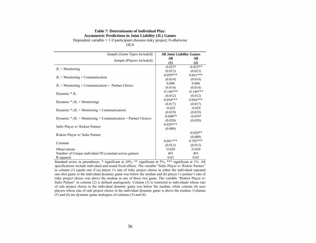
In Table 7, we examine our asymmetric predictions about the impact of joint

liability contract structure on different types of players. In columns (1) and (2), we focus

on heterogeneous pairings. The variables “Safer Player w/ Riskier Partner” and “Riskier

Player w/ Safer Partner” are defined as follows: we termed a player “safer” (“riskier”) if

she chose the risky project with less (greater) than the median frequency in the individual

liability games; the variable “Safer Player w/ Riskier Partner” (“Riskier Player w/ Safer

Partner”) is a dummy equal to one if a player is safer (riskier) and her partner is riskier

(safer) by this definition. As predicted, column (1) shows that safe types do increase their

rates of risky project choice when they are matched with risky partners, though at only

three percent the effect is relatively small. Column (2) indicates that risky players are

somewhat less likely to invest in the risky project when they are matched with a safe

individual, providing evidence of coordination, altruism, or both.

6.2 Coordination

The effects of the behavioral changes described above on joint outcomes and default rates

are indeterminate since they depend on the nature of pairings, and that depends on the

initial distribution of risk preference types, beliefs about this distribution, and the

outcome of the random group formation process. For example, joint liability might

decrease default rates in a uniformly risk neutral population, since partners would be

forced to insure one another. Alternatively, all of the contractual mechanisms we consider

might have no effect on a uniformly risk averse population – one in which it was known

that everyone preferred the safe investment to the risky option in the individual game –

since, in that population, everyone would play safe. Finally, joint liability contract

21

structures might lead to increased default if players move toward risky behavior when

they expect to repay the loans of their partners with positive probability.

Table 8 considers joint outcomes using a multinomial logit specification with

three possible values for the dependent variable: both played risky, played opposite, and

both played safe (the omitted category). Allowing communication in the repeated one-

shot games greatly increases the rate of both playing risky, a result that is profit

maximizing given the lack of penalty for default. In the dynamic games with

communication, we see a substantial increase in both playing opposite (i.e., risky-safe)

and both playing risky. Playing opposite is consistent with the strategy of profit

maximization while protecting the ability to continue playing.

Strikingly, in the dynamic games, allowing for endogenous partner choice sharply

decreases the rate of joint risky play and the rate of mixed play. The result is a strong

increase in jointly safe choices. This is a result to which we return below in Section 6.4

(Partner Choice).

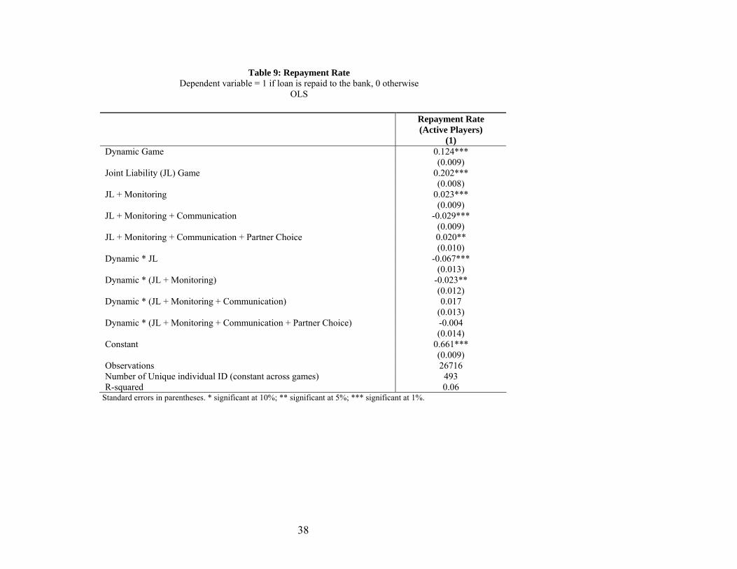
Table 9 considers the outcome of interest to the bank – repayment. The table

examines the effect of loan contract structure on repayment among those actively taking

out loans in any given round (i.e. excluding those who are no longer playing because they

have defaulted in an earlier round of a dynamic game). Not surprisingly, dynamic

incentives, joint liability, monitoring and endogenous partner choice all increase

repayment in this framework. Communication, on the other hand, leads to higher default

rates due to the increase in jointly risky play shown in Table 8.

6.3 Punishment

We introduced an opportunity for ex post punishment in the dynamic monitoring games.

In these games, communication was not allowed and anonymity was maintained

throughout. In “punishment games,” participants learned at the beginning of the game

that they would be allowed to punish their partners at the end of the game. After the

completion of each punishment game, each participant was given an opportunity to pay

50 points and deduct 500 points from the final point total of her partner.

22

Several models of joint liability (e.g. Besley and Coate 1995) suggest that it

increases repayment because villagers can punish default with social sanctions. Though

social sanctions are not feasible in a laboratory environment, previous studies have found

that participants in experiments are often willing to pay to punish uncooperative behavior

in the lab, despite the fact that such punishment is not part of any subgame perfect

equilibrium (Fehr and Gächter 2000).

In total, 380 players participated in punishment games, and 61 of these players

punished a partner. Since theory suggests that punishment can only occur out of

equilibrium, the observed frequency is unexpectedly high: the mere threat of punishment

should drive behavioral changes, and we should not actually observe punishment. On the

other hand, if we expect all safe players to punish risky choices by their partners, the

punishment rate is low.

Table 4 shows that adding punishment leads to a slight increase in risk-taking – to

53 percent from 47 percent in the joint liability dynamic games with monitoring – and a

modest drop in the average repayment rate – to 93 percent from 95. In principle,

punishment should help steer coordination, but the summary statistics in Table 4 are too

aggregated to reveal the specific dynamics. Table 10 explores specific hypotheses around

coordination. Analyses of punishment treatments are completed using OLS and a

multinomial logit. In the multinomial logit, we use the dependent variables “both played

risky,” “both played safe,” and “played opposite” that were defined above. Table 10

shows that adding the possibility of punishment significantly reduces rates of joint risky

play and has little effect on opposite play. Implicitly, the action arises from an increase in

the omitted category (joint safe play). This leads to a slightly lower default rate for the

lender (column 1). Note that the regression results with fixed effects in Table 10 are

inconsistent with the summary statistics from Table 4. The discrepancy could be due to

the introduction of the fixed effects, and hence the preferred analysis is that from Table

10, that shows that punishment leads to safer play.

23

6.4 Partner choice

As Tables 5 and 7 demonstrate, allowing participants to choose their own partners has a

strong, negative effect on risk-taking. Table 11 begins to address the issue by examining

the determinants of matching among players by running social network regressions. For

each communication game (where partners are either elected or assigned), we create all

possible dyads or pairs among players: if a game has twenty players, there are 190

possible pairs or combinations of two players. However, only ten of those pairs are

matches, either randomly assigned by the computer or elected by the players

themselves.10 The goal is to determine the relevant variables used by players in choosing

their partners. We use the information on where players were sitting during the games,

whether they had ever been guests or hosts,11 the social network survey, and the census

survey.

Columns (2), (3) and (4) report the results for all elected partner games, broken

down into one-shot and dynamic treatments. For comparison purposes, column (1)

reports the results of the network regression using the randomly assigned matches from

the other communication treatment (without endogenous partner choice) as dependent

variable. By comparing the R-squared of the elected partner games to that of the assigned

partner manipulations, it is clear individuals match on information that is observable to

the econometrician – there is a much better fit when players can choose their partner.

The coefficient on “sitting next to your partner” is only significant (taking a

negative sign) when the partner is assigned. This reflects the fact that the random

assignment process avoided pairing individuals who were sitting next to each other (so

that they could not share information and infer they were matched). In contrast, having

10 Dyadic observations are typically not independent due to the presence of individual-specific factors common to all observations involving the individual. Thus, OLS or probit methods will yield inconsistent standard errors. We use game and player fixed effects to correct for this problem. Another method used in the literature, especially among sociologists, is the Quadratic Assignment Procedure (QAP). This method, similar to bootstrap, computes the p-value directly. We compared both fixed effects estimates and QAP estimates and found them very similar. Thus, we only report fixed effects estimates. 11 On certain days, participation was restricted to individuals that had already played (hosts) who were allowed to attend only if they invited someone that had never played (a guest).

24

been a host or a guest of someone else is an important predictor of partner choice.12

Despite its correlation with some social network questions, these questions have

predictive power on their own, even when census variables are introduced. While

participants tend to sort along most social network variables in one-shot games, fewer

variables predict pairing in the dynamic games: being relatives and having watched the

partner’s store are the only significant predictors from the social networks data in the

dynamic treatments.

The most notable finding is a non-result: there is no evidence that risk averse

partners particularly choose each other in the dynamic games. Not being risk averse has

some explanatory power, but the coefficient (0.048) is considerably smaller than other

variables like being a relative or having watched a partner’s store.13 These data thus offer

little support for Ghatak’s (1999) hypothesis that joint liability will lead to assortative

matching by risk attributes.

The findings reinforce the puzzle: if pairing is done mainly on the basis of social

attributes, the ability to coordinate on mixed risky-safe project choices (and thus to

increase earnings) should be enhanced. It should be easier to coordinate among people

who know each other well, and, with anonymity dropped, enforcement mechanisms that

operate outside of the game setting may come into play. But instead we see a tendency

toward safe-safe choices.

It cannot simply be that partners who know each other enjoy playing the game

together and thus opt for longevity in the game over maximizing point totals: the mixed

safe-risky option also guarantees longevity. One possibility is that participants judge their

success relative to their close friends and relatives; in this case, they may prefer to

coordinate at a low, safe level in which equal point totals are guaranteed, rather than

risking the chance of imbalanced totals when trying to coordinate on risky-safe choices.

12 Using the same methods we regressed “Had ever been a host or guest” against social network variables as well as census variables and found (not shown) that host and guest pairs tended to be between individuals that sold the same product, were relatives or close friends, that is, people that trusted each other and knew each other well. 13 In general matched players do not have the same marital status, but given that being relatives is so important, it could be that parents and children play together, explaining the difference in marital status (and possibly the same religion).

25

Another possibility is that participants that would otherwise choose the risky project, play

instead safe in an attempt to be fair to their friends (Rabin 1993; Fehr and Schmidt 1999).

Stiglitz (1990) assumes that partner selection allows coordination to the efficient

outcome. In contrast, we find that communication introduces a social element that results

in a sub-optimal level of risk-taking, albeit only in the dynamic treatment. The

explanation, with its stress on the desire for equality of outcomes, points to a downside of

joint liability: that it can induce a set of choices that is more conservative than optimal.

7 Conclusion Microfinance is transforming thinking about banking in low-income communities. The

techniques that are employed to ensure loan repayment contain numerous overlapping

mechanisms, and we have taken them apart in order to examine how important

components function in isolation and how they interact with one another.

The results draw from a series of experimental “microfinance games” run over

seven months in Peru. The experimental laboratory approach allows us to pose clear but

narrow questions and generate precise hypotheses about several loan features all at once.

Furthermore, by locating the games in Peru, we were also able to attract participants who

are similar to typical microfinance customers, including some who were in fact customers

of local microfinance institutions.

Our focus has been on group-based mechanisms. We describe a balancing act.

Joint liability reduces default since group members bail each other out when luck is

bad.14 Thus, ceteris paribus, group-based mechanisms help the lender’s bottom line. But

the mechanisms can also generate riskier behavior on the part of borrowers, undermining

some of the lender’s gains. Our findings here confirm the existence of a puzzle that is

often overlooked in theoretical models of group-based lending: the group-based

mechanisms that are frequently employed can induce moral hazard (or more risk-taking

behavior) instead of reducing it. Moreover, improving the information flows between

14 Although, as Rai and Sjöström (2004) show, insurance could also be achieved through side contracts in an individual liability setting.

26

members can make matters even worse. However, we show that allowing participants to

form groups can help to mitigate these tendencies – through assortative matching, the

positive features of group banking can be established. This, though, introduces its own

puzzle: risk-taking falls to levels that are surprisingly low.

Apart from this insight into joint liability mechanisms, we also found that

dynamic incentives are powerful tools for reducing moral hazard even when lenders are

using individual liability contracts. These results are consistent with recent shifts by

micro-lenders from group-based mechanisms toward individual loans. The Grameen

Bank of Bangladesh and Bolivia’s BancoSol, for example, are the two best-known group

lending pioneers, but they have both shifted toward individual lending as their customers

have matured and sought larger loans (Armendariz de Aghion and Morduch 2005).

Grameen has dropped joint liability entirely, and just one percent of BancoSol’s loan

portfolio was under group contracts in 2005. The individual-lending approach allows

customers and lenders more flexibility without the worry about the moral hazard induced

by the use of groups. Giné and Karlan (2006) conduct a natural field experiment in the

Philippines in which pre-formed group liability centers were assigned randomly to be

converted to individual-liability centers (treatment group) or to remain as-is (control

group) in order to test the importance of group liability for mitigating moral hazard. They

find no change in default rate under individual liability relative to group liability and an

increase in ability to attract new clients. Hence, the group liability contract does not

appear to be a necessary component of the microfinance model in order to maintain high

repayment rates.

The participants in these games behaved strategically according to predictions

drawn from neo-classical theories of choice under risk, but participants were also

sensitive to social factors of the simulated credit contracts. Ultimately, these

microfinance games show how strategic behavior and social concerns interact to yield

effective contracts that can work both for customers and lenders. But there is evidence

that the social factors undermine profit maximization by customers and may blunt the

effectiveness of group-based approaches in reducing poverty and stimulating investment.

27

References Armendariz de Aghion, B. and J. Morduch (2000). "Microfinance Beyond Group

Lending." Economics of Transition 8(2): 401-420. Armendariz de Aghion, B. and J. Morduch (2005). The Economics of Microfinance, MIT

Press. Banerjee, A., T. Besley and T. Guinnane (1994). "Thy Neighbor's Keeper: The Design of

a Credit Cooperative with Theory and a Test." Quarterly Journal of Economics 109(2): 491-515.

Barr, A. M. and B. Kinsey (2002). "Do Men Really Have No Shame?" Oxford University working paper.

Besley, T. J. and S. Coate (1995). "Group Lending, Repayment Incentives and Social Collateral." Journal of Development Economics 46(1): 1-18.

Brehm, J. and W. M. Rahn (1997). "Individual-level evidence for the causes and consequences of social capital." American Journal of Political Science 41(3): 999-1024.

Cassar, A., L. Crowley and B. Wydick (2005). "The Effect of Social Capital on Group Loan Repayment: Evidence from Artefactual Field Experiments." working paper.

de Meza, D. and D. Webb (1990). "Risk, Adverse Selection and Capital Market Failure." Economic Journal 100(399): 206-214.

Fehr, E. and S. Gächter (2000). "Cooperation and Punishment in Public Goods Experiments." American Economic Review 90(4): 980-994.

Fehr, E. and K. M. Schmidt (1999). "A Theory of Fairness, Competition, and Cooperation." Quarterly Journal of Economics 114: 817–68.

Fisman, R. and T. Khanna (1999). "Is Trust a Historical Residue? Information Flows and Trust Levels." Journal of Economic Behavior and Organization 38: 79-92.

Ghatak, M. (1999). "Group lending, local information and peer selection." Journal of Development Economics 60(1): 27-50.

Giné, X. and D. Karlan (2006). "Group versus Individual Liability: Evidence from a Field Experiment in the Philippines." working paper.

Gruber, J. (2005). Public Finance and Public Policy. New York, Worth Publishers. Harrison, G. and J. A. List (2004). "Field Experiments." Journal of Economic Literature

XLII: 1009-1055. Karlan, D. S. (2005a). "Social Connections and Group Banking." Yale University

Economic Growth Center Discussion Paper 913. Karlan, D. S. (2005b). "Using Experimental Economics to Measure Social Capital and

Predict Financial Decisions." American Economic Review 95(5): 1688-1699. Karlan, D. S. and J. D. Zinman (2005). "Observing Unobservables: Identifying

Information Asymmetries with a Consumer Credit Field Experiment." Yale University Economic Growth Center Discussion Paper 911.

Kennedy, B. P., I. Kawachi, D. Prothrow-Stith and K. Lochner (1998). "Social capital, income inequality, and firearm violent crime." Social Science and Medicine 47(1): 7-17.

28

Knack, S. F. and P. Keefer (1997). "Does Social Capital Have an Economic Payoff? A Cross-Country Investigation." Quarterly Journal of Economics November 1997: 1251-1288.

Lazear, E., U. Malmendier and R. Weber (2005). "Sorting in Experiments." working paper.

Lederman, D., N. V. Loayza and A. M. Menendez (2002). "Crime: Does Social Capital Matter?" Economic Development and Cultural Change 50(3): 509-539.

List, J. A. (2004). "Neoclassical Theory Versus Prospect Theory: Evidence from the Marketplace." Econometrica 72(2): 615-625.

Menon, N. (2003). "Consumption Smoothing in Micro-credit Programs." Review of Economics and Statistics forthcoming.

Rabin, M. (1993). "Incorporating Fairness into Game Theory and Economics." American Economic Review 85(5): 1281-1302.

Rai, A. and T. Sjöström (2004). "Is Grameen Lending Efficient? Repayment Incentives and Insurance in Village Economies." Review of Economic Studies 71(1): 217-234.

Sadoulet, L. (2000). The Role of Mutual Insurance in Group Lending., ECARES/Free University of Brussels.

Stiglitz, J. (1990). "Peer Monitoring and Credit Markets." World Bank Economic Review 4(3): 351-366.

Wydick, B. (1999). "Can Social Cohesion be Harnessed to Repair Market Failures? Evidence from Group Lending in Guatemala." Economic Journal 109(457): 463-475.

Yunus, M. (1999). Banker to the Poor. New York, Public Affairs.

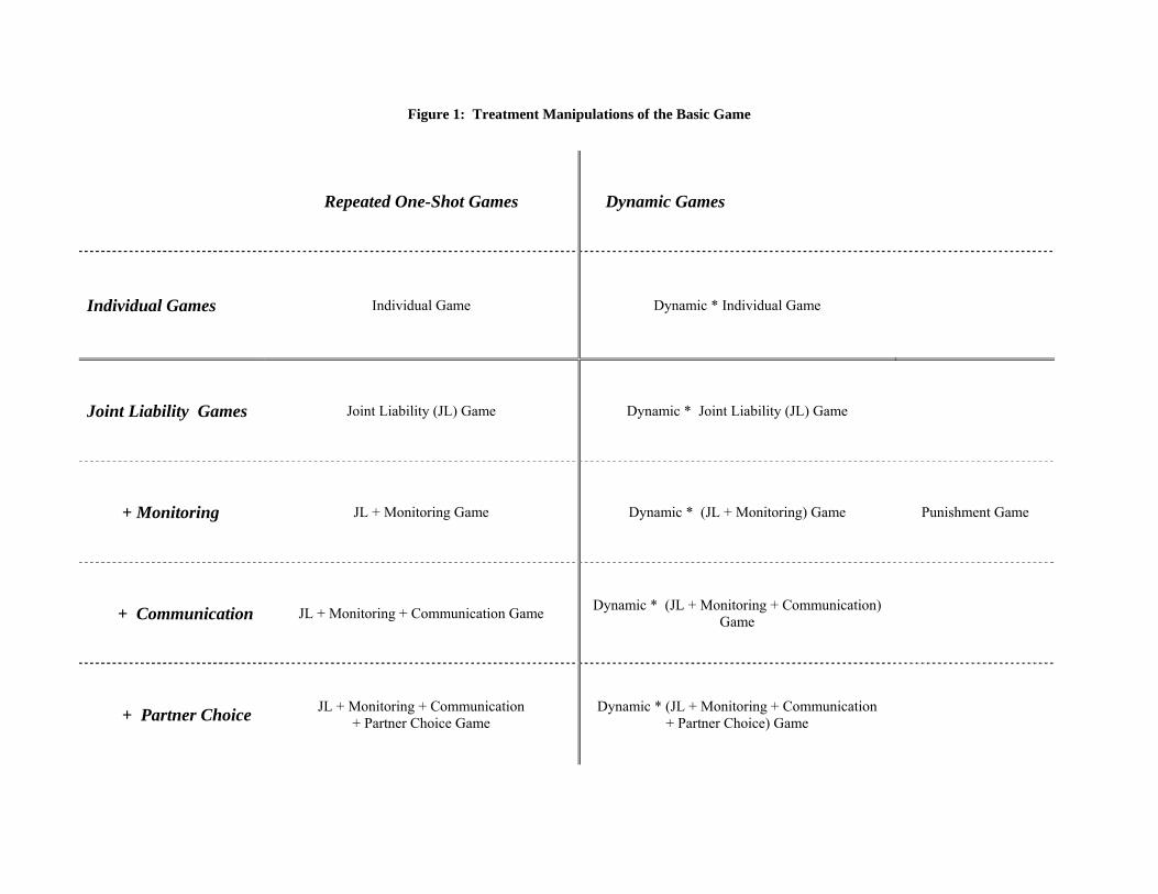
Figure 1: Treatment Manipulations of the Basic Game

Repeated One-Shot Games Dynamic Games

Individual Games Individual Game Dynamic * Individual Game

Joint Liability Games Joint Liability (JL) Game Dynamic * Joint Liability (JL) Game

+ Monitoring JL + Monitoring Game Dynamic * (JL + Monitoring) Game Punishment Game

+ Communication JL + Monitoring + Communication Game Dynamic * (JL + Monitoring + Communication) Game

+ Partner Choice JL + Monitoring + Communication + Partner Choice Game

Dynamic * (JL + Monitoring + Communication + Partner Choice) Game

Table 1: Net Payouts each Round in Joint Liability Games

Decision-Maker’s Choice

Partner’s Choice

Decision-Maker’s Outcome

Partner’s Outcome Probability Net Payout Default?

Safe

+ + 100% 100 No

■: Safe Project

Risky

+ + -

50 50

100 0

No No

Safe

+ - + 50

50 500

0 No No

▲: Risky Project

Risky + -

+ - + -

25 25 25 25

500 400

0 0

No No No Yes

31

Table 2: Treatment Manipulations

Total Number of Games Played

Average Number of Players / Game

Repeated One-Shot Games

Dynamic Games

Repeated One-Shot Games

Dynamic Games

Individual Games

34 37 19.3 20.2

Joint Liability

31 33 21.6 19.7

Joint Liability + Monitoring

32 28 18.6 19.3

Joint Liability + Monitoring + Communication

22 25 20.2 20.7

Joint Liability + Monitoring + Communication + Partner Choice

25 23 20.5 18.3

Joint Liability + Monitoring + Punishment

N.A.

32

N.A.

13.1

32

Table 3: Summary Statistics on Player and Market Demographic Characteristics

Entire Census Sample Participants in Games

Mean Standard error Mean Standard error Female 0.58 (0.49) 0.57 (0.50) Age 29.9 (10.5) 34.4 (11.9) Married 0.39 (0.49) 0.49 (0.50) Years of education 5.6 (1.1) 5.6 (1.15) Spanish is second language 0.08 (0.27) 0.11 (0.31) Attends church at least once a week 0.22 (0.41) 0.28 (0.45) Does not attend church 0.10 (0.30) 0.05 (0.21) Born in Lima 0.53 (0.50) 0.51 (0.50) Household size 4.7 (2.3) 4.9 (2.1) Number of assets / appliances 3.1 (1.7) 2.9 (1.6) Cooks with kerosene 0.08 (0.26) 0.11 (0.32) Played lotto in past month 0.19 (0.39) 0.18 (0.38) Visited casino in past month 0.07 (0.26) 0.06 (0.24) Number of positive GSS answers 0.33 (0.59) 0.40 (0.67) Years experience 8.2 (7.9) 11.4 (9.2) Owns microenterprise 0.34 (0.48) 0.51 (0.50) Hours worked per week 65.8 (15.6) 63.3 (19.8) Number of workers in business 1.9 (0.9) 2.3 (1.0) Has government business license 0.73 (0.44) 0.62 (0.49) Saves in a commercial bank 0.09 (0.28) 0.07 (0.26) Has been involved in a ROSCA 0.61 (0.49) 0.65 (0.48) Has had a joint liability loan 0.03 (0.17) 0.06 (0.24) Received a loan in past year 0.28 (0.45) 0.39 (0.49) Observations 1427 323

33

Table 4: Summary Statistics: Average Rates of Risky Choices and Repayment

Percent of Participants Choosing Risky Investment Repayment Rate (Percent)

Repeated One-Shot games

Dynamic Games

Repeated One-Shot Games

Dynamic Games

Individual Games

61 34 68 82

Joint Liability

63 49 88 94

Joint Liability + Monitoring

61 47 90 95

Joint Liability + Monitoring + Communication

68 58 87 91

Joint Liability + Monitoring + Communication + Partner Choice

69 53 89 94

Joint Liability + Monitoring + Punishment N.A. 53 N.A. 94

34

Table 5: Determinants of Risky Choice by Individuals: Implications of Contract Structure Dependent Variable = 1 if participant chooses risky project, 0 otherwise

OLS

Sample: All Games

Repeated One-Shot

Games Dynamic Games

(1) (2) (3) Dynamic Game -0.213*** (0.013) Joint Liability (JL) Game 0.015 0.022* (0.012) (0.012) JL + Monitoring -0.023* -0.023* (0.012) (0.012) JL + Monitoring + Communication 0.061*** 0.060*** (0.013) (0.014) JL + Monitoring + Communication + Partner Choice 0.007 0.007 (0.013) (0.014) Dynamic * JL 0.065*** 0.072*** (0.018) (0.014) Dynamic * (JL + Monitoring) 0.056*** 0.022* (0.017) (0.012) Dynamic * (JL + Monitoring + Communication) -0.028 0.044*** (0.018) (0.013) Dynamic * (JL + Monitoring + Communication + Partner Choice) -0.037* -0.035** (0.020) (0.015) Previous days played Constant 0.666*** 0.651*** 0.484*** (0.012) (0.012) (0.015) Observations 26716 13541 13175 Number of Unique individual ID (constant across games) 493 474 449 R-squared 0.04 0.01 0.03 Standard errors in parentheses. * significant at 10%; ** significant at 5%; *** significant at 1%. Individual and round fixed effects included in all specifications.

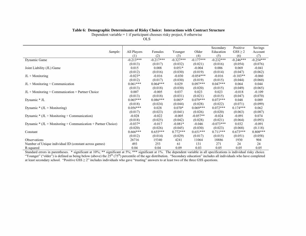
Table 6: Demographic Determinants of Risky Choice: Interactions with Contract Structure Dependent variable = 1 if participant chooses risky project, 0 otherwise

OLS

Sample: All Players Females Younger Older Secondary Education

Positive GSS ≥ 2

Savings Account

(1) (2) (3) (4) (5) (6) (7) Dynamic Game -0.213*** -0.217*** -0.327*** -0.177*** -0.232*** -0.246*** -0.254*** (0.013) (0.017) (0.032) (0.021) (0.016) (0.054) (0.076) Joint Liability (JL) Game 0.015 0.008 0.051* -0.004 0.006 0.069 -0.041 (0.012) (0.016) (0.030) (0.019) (0.014) (0.047) (0.062) JL + Monitoring -0.023* -0.016 -0.030 -0.054*** -0.016 -0.103** -0.060 (0.012) (0.017) (0.030) (0.019) (0.015) (0.044) (0.060) JL + Monitoring + Communication 0.061*** 0.064*** 0.029 0.097*** 0.047*** 0.064 0.044 (0.013) (0.018) (0.030) (0.020) (0.015) (0.049) (0.065) JL + Monitoring + Communication + Partner Choice 0.007 -0.005 0.037 0.023 0.023 -0.018 -0.109 (0.013) (0.018) (0.031) (0.021) (0.015) (0.047) (0.070) Dynamic * JL 0.065*** 0.086*** 0.085* 0.079*** 0.073*** 0.048 0.089 (0.018) (0.024) (0.044) (0.028) (0.022) (0.071) (0.099) Dynamic * (JL + Monitoring) 0.056*** 0.028 0.070* 0.069*** 0.072*** 0.174*** 0.062 (0.017) (0.023) (0.041) (0.026) (0.020) (0.063) (0.087) Dynamic * (JL + Monitoring + Communication) -0.028 -0.022 -0.005 -0.057** -0.024 -0.091 0.074 (0.018) (0.025) (0.042) (0.028) (0.021) (0.064) (0.093) Dynamic * (JL + Monitoring + Communication + Partner Choice) -0.037* -0.017 -0.081* -0.046 -0.073*** 0.032 -0.091 (0.020) (0.026) (0.045) (0.030) (0.023) (0.068) (0.118) Constant 0.666*** 0.655*** 0.772*** 0.651*** 0.711*** 0.673*** 0.808*** (0.012) (0.014) (0.029) (0.017) (0.015) (0.051) (0.058) Observations 26716 15340 4241 11064 18886 1930 904 Number of Unique individual ID (constant across games) 493 253 61 131 271 24 24 R-squared 0.04 0.04 0.09 0.03 0.05 0.05 0.05 Standard errors in parentheses. * significant at 10%; ** significant at 5%; *** significant at 1%. The dependent variable in all specifications is individual risky choice. “Younger” (“older”) is defined as being below (above) the 25th (75th) percentile of the age distribution. “Secondary education” includes all individuals who have completed at least secondary school. “Positive GSS ≥ 2” includes individuals who gave “trusting” answers to at least two of the three GSS questions.

36

Table 7: Determinants of Individual Play: Asymmetric Predictions in Joint Liability (JL) Games

Dependent variable = 1 if participant chooses risky project, 0 otherwise OLS

Sample (Game Types Included): All Joint Liability Games

All All Sample (Players included): (1) (2) -0.023* -0.025** JL + Monitoring (0.013) (0.013)

0.059*** 0.061*** JL + Monitoring + Communication (0.014) (0.014) 0.008 0.006 JL + Monitoring + Communication + Partner Choice (0.014) (0.014)

-0.146*** -0.146*** Dynamic * JL (0.012) (0.012) 0.054*** 0.056*** Dynamic * (JL + Monitoring) (0.017) (0.017)

-0.025 -0.029 Dynamic * (JL + Monitoring + Communication) (0.019) (0.019) -0.040** -0.039* Dynamic * (JL + Monitoring + Communication + Partner Choice) (0.020) (0.020) 0.029*** Safer Player w/ Riskier Partner (0.009)

-0.020** Riskier Player w/ Safer Partner (0.008) 0.681*** 0.703*** Constant (0.013) (0.013)

Observations 21420 21420 Number of Unique individual ID (constant across games) 491 491 R-squared 0.03 0.03

Standard errors in parentheses. * significant at 10%; ** significant at 5%; *** significant at 1%. All specifications include individual and round fixed effects. The variable “Safer Player w/ Riskier Partner” in column (1) equals one if (a) player i’s rate of risky project choice in either the individual repeated one-shot game or the individual dynamic game was below the median and (b) player i’s partner’s rate of risky project choice was above the median in one of those two game. The variable “Riskier Player w/ Safer Partner” in column (2) is defined analogously. Column (3) is restricted to individuals whose rate of safe project choice in the individual dynamic game was below the median, while column (4) uses players whose rate of safe project choice in the individual dynamic game is above the median. Columns (5) and (6) are dynamic game analogues of columns (3) and (4).

37

Table 8: Determinants of Joint Outcomes Multinomial Logit

Treatments Included: Repeated One-Shot

Games Only Dynamic Games Only

Specification: Multinomial Logit Multinomial Logit Omitted Outcome: Both Played Safe Both Played Safe

(1) (2) Outcome #1: Both Played Risky Both Played Risky

Monitoring -0.097 0.085 (0.098) (0.093) Monitoring + Communication 0.385*** 0.598*** (0.110) (0.103) Monitoring + Communication + Partner Choice 0.038 -0.433*** (0.112) (0.121) Constant 0.250 28.978*** (1.423) (1.654)

Outcome #2: Played Opposite Played Opposite Monitoring 0.035 0.076 (0.093) (0.073) Monitoring + Communication 0.053 0.482*** (0.108) (0.085) Monitoring + Communication + Partner Choice 0.054 -0.207** (0.112) (0.100) Constant 1.289 28.464*** (1.126) (1.428) Observations 10554 10166 Fixed Effects of Individuals Yes Yes R-squared 0.15 0.16 Standard errors in parentheses. * significant at 10%; ** significant at 5%; *** significant at 1%.

38

Table 9: Repayment Rate Dependent variable = 1 if loan is repaid to the bank, 0 otherwise

OLS

Repayment Rate (Active Players)

(1) Dynamic Game 0.124*** (0.009) Joint Liability (JL) Game 0.202*** (0.008) JL + Monitoring 0.023*** (0.009) JL + Monitoring + Communication -0.029*** (0.009) JL + Monitoring + Communication + Partner Choice 0.020** (0.010) Dynamic * JL -0.067*** (0.013) Dynamic * (JL + Monitoring) -0.023** (0.012) Dynamic * (JL + Monitoring + Communication) 0.017 (0.013) Dynamic * (JL + Monitoring + Communication + Partner Choice) -0.004 (0.014) Constant 0.661*** (0.009) Observations 26716 Number of Unique individual ID (constant across games) 493 R-squared 0.06

Standard errors in parentheses. * significant at 10%; ** significant at 5%; *** significant at 1%.

39

Table 10: Effect of Punishment Opportunity on Outcomes OLS, Multinomial Logit

Dependent variable:

Default

Both Played Risky

Played Opposite Specification: OLS Multinomial Logit

(1) (2) (3) -0.015* -0.308*** -0.050

Punishment Game (0.008) (0.091) (0.078)

0.084*** 1.386 1.946* Constant

(0.003) (1.118) (1.069) Observations 12814 12404 12404 Fixed Effects of Individuals Yes Yes Yes R-squared 0.00 0.00 0.00 Standard errors in parentheses. * significant at 10%; ** significant at 5%; *** significant at 1%. In all specifications, the sample is restricted to dynamic joint liability games with monitoring. Columns 2 and 3 report the results from one multinomial logit specification, where “Both played safe” is the omitted outcome.

Table 11: Determinants of Partner Choice Dependent variable = 1 if dyad is partnered

OLS Elected Partners

Assigned Partners All games

Repeated One-Shot

Games Dynamic games

(1) (2) (3) (4) Sitting next to each other -0.0722*** 0.0097 0.0184 -0.0013 (0.0145) (0.0138) (0.0176) (0.0227) Has ever been host or guest of partner -0.0545 0.4720*** 0.6255*** 0.2389*** (0.0349) (0.0322) (0.0395) (0.0555) From Social Networks Survey Bought or sold from partner's store -0.0065 0.0134 0.0166 0.0129 (0.0123) (0.0124) (0.0157) (0.0210) Is relative of partner -0.0038 0.1971*** 0.2019*** 0.2029*** (0.0361) (0.0340) (0.0480) (0.0507) Coincides in social gathering with partner -0.0194 0.0254* 0.0384** 0.0004 (0.0126) (0.0131) (0.0168) (0.0217) Knows store location of partner 0.0321*** 0.0256** 0.0271* 0.0222 (0.0116) (0.0126) (0.0153) (0.0221) Has watched over store for partner 0.0347*** 0.0906*** 0.0857*** 0.1039*** (0.0129) (0.0127) (0.0163) (0.0208) Both are popular -0.0021 -0.0271** -0.0171 -0.0392 (0.0123) (0.0123) (0.0157) (0.0242) Both are trusted 0.0068 -0.0155 -0.0164 -0.0045 (0.0112) (0.0111) (0.0139) (0.0211) From Census Survey Both are highly risk averse -0.0077 -0.0085 -0.0224 0.0011 (0.0195) (0.0189) (0.0239) (0.0313) Both are moderately risk averse 0.0314 -0.0234 -0.0067 -0.0505 (0.0215) (0.0215) (0.0262) (0.0384) Both are not risk averse -0.0161 0.0375** 0.0290 0.0478* (0.0175) (0.0167) (0.0207) (0.0284) Both have same marital status -0.0004 -0.0163** -0.0082 -0.0277** (0.0089) (0.0081) (0.0102) (0.0136) Both share same religion -0.0012 0.0380*** 0.0423*** 0.0375* (0.0121) (0.0118) (0.0148) (0.0200) Wealth difference 0.0160*** -0.0107* -0.0138* -0.0077 (0.0062) (0.0062) (0.0079) (0.0103) Polvos Azules founder 0.0134 0.0357** 0.0419** 0.0329 (0.0157) (0.0153) (0.0192) (0.0257) Both own the store -0.0180 0.0008 0.0357* -0.0578* (0.0179) (0.0173) (0.0216) (0.0296) Constant -0.3474 -0.1530 -0.1423 -0.0021 (0.4096) (0.5271) (0.5038) (0.3232) Observations 3,610 3,426 1,985 1,441 R-squared 0.0501 0.1887 0.2520 0.1722

Standard errors in parenthesis. * significant at 10%; ** significant at 5%; *** significant at 1%. The dependent variable is a binary variable with value one if the dyad is a match. “Sitting adjacent to each other” takes value one if both players in the dyad are sitting next to each other. “Has ever been host or guest of partner” equals one if player was ever been a guest or host of the partner in days where participation was restricted to individuals that had previously played as long as they invited an individual that had never played. All the variables from the social networks survey except for “both are popular” and “both are trusted” take value one if either player in the dyad answers positively to the statement when asked about partner. A player is popular if the number of participants that know the name or store location of the player is higher than that of the median player. Likewise, a player is trusted if the number of participants that report having watched the store or being related to the players is higher than that of the median player. “Both are popular” (“both are trusted”) takes the value one if both players are popular (trusted), and takes the value zero otherwise. Risk aversion questions come from the experimental questions in the survey. The regressions include game and individual fixed effects.

Appendix Table 1: Determinants of Participation in Games OLS

Dependent Variable: Played Games at Least Once Days Played Sample: Entire Census Owners Non-Owners Entire Census

(1) (2) (3) (4) Female 0.014 0.029 0.016 0.454 (0.023) (0.047) (0.024) (0.493) Age 0.005*** 0.003 0.006*** 0.116*** (0.002) (0.003) (0.002) (0.036) Married -0.019 -0.018 -0.029 -0.238 (0.025) (0.048) (0.026) (0.532) Years of education 0.003 0.003 0.000 0.015 (0.005) (0.009) (0.007) (0.105) Spanish is second language -0.028 -0.014 -0.028 -0.929 (0.040) (0.065) (0.055) (0.900) Attends church at least once a week 0.019 -0.005 0.025 0.465 (0.027) (0.054) (0.030) (0.557) Does not attend church -0.074** -0.153* -0.039 -1.750* (0.035) (0.083) (0.036) (0.956) Born in Lima 0.043* 0.051 0.040 0.844 (0.024) (0.052) (0.025) (0.532) Household size -0.003 -0.019* 0.001 -0.067 (0.005) (0.012) (0.005) (0.111) Number of assets / appliances -0.017** -0.034** -0.009 -0.285* (0.007) (0.014) (0.008) (0.159) Cooks with kerosene 0.086* 0.060 0.080 1.194 (0.049) (0.096) (0.054) (0.846) Played lotto in past month -0.003 -0.037 0.022 -0.273 (0.032) (0.063) (0.038) (0.704) Visited casino in past month -0.017 -0.137 0.003 -0.057 (0.044) (0.092) (0.043) (0.957) Number of positive GSS answers 0.043** 0.036 0.047*** 0.982*** (0.017) (0.039) (0.018) (0.375) Years experience 0.002 0.002 0.006** 0.059 (0.002) (0.003) (0.003) (0.043) Owns microenterprise 0.073** 1.115* (0.029) (0.591) Hours worked per week -0.001 0.000 -0.001* -0.020 (0.001) (0.001) (0.001) (0.014) Number of workers in business 0.091*** 0.083*** 0.080*** 2.002*** (0.012) (0.030) (0.012) (0.259) Has government business license -0.058** -0.132*** -0.006 -1.186** (0.026) (0.048) (0.029) (0.523) Saves in a commercial bank -0.033 -0.152** 0.037 -1.449 (0.038) (0.070) (0.048) (0.900) Has been involved in a ROSCA 0.020 0.064 0.002 0.134 (0.023) (0.047) (0.025) (0.511) Has had a joint liability loan 0.097 0.198* 0.033 1.949 (0.076) (0.103) (0.130) (1.221) Received a loan in past year 0.086*** 0.098** 0.063* 1.938*** (0.027) (0.046) (0.032) (0.519) Constant -11.765*** (2.279) Pseudo R2 0.14 0.11 0.16 0.07 Observations 1418 488 930 1418 Robust standard errors in parentheses. * significant at 10%; ** significant at 5%; *** significant at 1%. Columns (1) through (3) are probit regressions in which the dependent variable is equal to one if an individual ever participated in the microfinance games (marginal effects reported). Column (4) is a tobit regression in which the dependent variable is the number of times an individual participated in the games. The independent variable “number of assets / appliances” aggregates seven survey questions which asked whether individuals owned a land line telephone, a cell phone, a computer, a car, a washing machine, a television with a remote control, or a refrigerator.

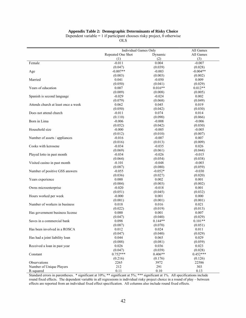
42

Appendix Table 2: Demographic Determinants of Risky Choice Dependent variable = 1 if participant chooses risky project, 0 otherwise

OLS

Individual Games Only All Games Repeated One Shot Dynamic All Games (1) (2) (3) Female -0.011 0.004 -0.007 (0.047) (0.039) (0.028) Age -0.007** -0.003 -0.004** (0.003) (0.003) (0.002) Married 0.041 -0.050 0.009 (0.050) (0.041) (0.029) Years of education 0.007 0.016** 0.012** (0.009) (0.008) (0.005) Spanish is second language -0.029 -0.024 0.002 (0.079) (0.068) (0.049) Attends church at least once a week 0.062 0.045 0.019 (0.050) (0.042) (0.030) Does not attend church -0.011 0.074 0.014 (0.110) (0.090) (0.066) Born in Lima -0.006 -0.008 -0.006 (0.052) (0.042) (0.030) Household size -0.000 -0.005 -0.005 (0.012) (0.010) (0.007) Number of assets / appliances -0.016 -0.007 0.007 (0.016) (0.013) (0.009) Cooks with kerosene -0.034 -0.035 0.026 (0.069) (0.061) (0.044) Played lotto in past month -0.034 -0.026 -0.015 (0.064) (0.054) (0.038) Visited casino in past month -0.101 -0.048 -0.003 (0.087) (0.080) (0.059) Number of positive GSS answers -0.055 -0.052* -0.030 (0.036) (0.027) (0.020) Years experience 0.000 0.002 0.001 (0.004) (0.003) (0.002) Owns microenterprise -0.020 -0.018 0.001 (0.051) (0.045) (0.032) Hours worked per week -0.000 0.001 0.000 (0.001) (0.001) (0.001) Number of workers in business 0.018 0.016 0.021 (0.022) (0.019) (0.013) Has government business license 0.000 0.001 0.007 (0.047) (0.040) (0.029) Saves in a commercial bank 0.098 0.144** 0.101** (0.087) (0.070) (0.051) Has been involved in a ROSCA 0.012 0.024 0.011 (0.047) (0.040) (0.029) Has had a joint liability loan 0.044 0.065 0.029 (0.088) (0.081) (0.059) Received a loan in past year 0.026 0.036 0.023 (0.047) (0.039) (0.028) Constant 0.752*** 0.406** 0.452*** (0.216) (0.176) (0.126) Observations 2265 3972 22586 Number of Unique Players 212 291 303 R-squared 0.11 0.10 0.13 Standard errors in parentheses. * significant at 10%; ** significant at 5%; *** significant at 1%. All specifications include round fixed effects. The dependent variable in all regressions is individual risky project choice in a round of play – between effects are reported from an individual fixed effect specification. All columns also include round fixed effects.

43

Appendix A: Game Administration All games were administered by a team of three to five researchers. Players were randomly assigned to numbered seats at the beginning of each game session, and were identified using their seat numbers throughout the day. In each game, each player received a packet of ten game worksheets. Sample worksheets are included in Appendix B. In each round, participants would circle their desired projects before returning their game packets to the researchers. Choices were then entered into a computer which randomized outcomes for players investing in the risky project and then reported individual earnings for that round (after automatically deducting the loan repayment). A member of the research team then highlighted final outcomes on participant game sheets before returning them to players. After players examined their results for the round, the game either continued into the next round or ended. Instructions Read to Participants Read at the beginning of all games: Good morning everyone. We are a group of college students carrying out research about how microentrepreneurs from Polvos Azules make business decisions. We would like you to participate in our study. If you choose to participate, we will ask you to play several types of games with us. Just for showing up and staying for two hours, you will receive ten soles. You may earn up to ten soles. How much you earn will depend on how many points you accumulate during the course of the games. The more points you accumulate during the games, the more money you will receive at the end of the session. Packets of game worksheets are passed out at this point. You are not allowed to talk to each other during the course of the games. In addition, you are not allowed to look at the worksheets of people sitting near you. Each game consists of multiple rounds. At the beginning of each round, you will receive a bank loan for 100 points. You must invest this loan in one of two projects: “Project Square” or “Project Triangle.” Project Square pays 200 points with certainty. If you choose Project Triangle, your project may be successful or it may fail. Each time you choose Project Triangle, it is like the computer flips an imaginary coin. If the coin lands on heads, you will receive 600 points. However, if the coin lands on tails, you won’t receive anything. Note that project outcomes are independent, so if two players chose Project Triangle in the same round, one can be successful while the other fails because the computer tosses a different imaginary coin for each player. Before receiving the points from your project, you have to repay the loan from the bank. This is done automatically by the computer, so no one has the right to decide whether or not to repay the loan. You can only use the points you earned in each round to repay the bank. In any round, if you choose Project Triangle and your project is not successful, you cannot repay the bank. To begin the game everybody is assigned 500 points. The only thing you have to do is circle one of the two projects for each round. After that you will hand us the game sheets and we will fill in the rest of the information after entering your choice into the computer. Do not forget to write your ID number in the upper right corner of each sheet. We will be playing many rounds, but we are not sure how many. It will be as if we were rolling an imaginary dice, and with some probability the game stops and we will start another game. There are going to be several types of games that we will explain as we play them. In some of them you will play alone, in others you will have a partner.

44

Read before specific game specifications: Individual Repeated One-Shot Games: In this game you will be playing alone, meaning you will be solely responsible for your loan from the bank. You will receive the loan from the bank and you will have to circle the project (Square or Triangle) that you want to invest in. In this game, you will always receive a new loan at the beginning of each round even when you were not able to repay your loan in the previous round. In this case, the bank will allow you to borrow again even if your project does not succeed and you do not repay the loan. Individual Dynamic Games: In this game you will be playing alone, meaning you will be solely responsible for your loan from the bank. You will receive the loan from the bank and you will have to circle the project (Square or Triangle) that you want to invest in. In this game, the bank will not loan to you again if your project does not succeed and thus are unable to repay the loan. This will happen if you choose Project Triangle and your project fails. In that case you will have to remain in your seat and wait for the other participants to finish playing. Joint Liability Repeated One-Shot Games: In this game you will be borrowing jointly from the bank with a partner in the room. You will not know who the partner is, nor will you be shown what project the partner chooses. As before, you will choose a project by circling either Square or Triangle. You and your partner are responsible for each other’s loans. If your project succeeds and your partner’s does not, you will have to repay your partner’s loan. On the other hand, if your partner’s project succeeds and yours does not, your partner will repay your loan. In this game, you will always receive a new loan at the beginning of each round even when neither of you are able to repay the loan in the previous round. Joint Liability Dynamic Games: In this game you will be borrowing jointly from the bank with a partner in the room. You will not know who the partner is, nor will you be shown what project the partner chooses. As before, you will choose a project by circling either Square or Triangle. You and your partner are responsible for each other’s loans. If your project succeeds and your partner’s does not, you will have to repay your partner’s loan. On the other hand, if your partner’s project succeeds and yours does not, your partner will repay your loan. In this game, the bank will not loan to you or your partner again if your projects do not succeed and you are unable to repay your loans. This will happen if both partners choose Triangle and both projects fail. Monitoring Repeated One-Shot Games: In this game you will be borrowing jointly from the bank with a partner in the room. You will not know who the partner is. However, at the start of each round, we will show you what your partner chose (square or triangle) in the prior round. As before, you will choose a project by circling either Square or Triangle. You and your partner are responsible for each other’s loans. If your project succeeds and your partner’s does not, you will have to repay your partner’s loan. On the other hand, if your partner’s project succeeds and yours does not, your partner will repay your loan. In this game, you will always receive a new loan at the beginning of each round even when neither of you are able to repay the loan in the previous round. Monitoring Dynamic Games: In this game you will be borrowing jointly from the bank with a partner in the room. You will not know who the partner is. However, at the start of each round, we will show you what your partner chose (square or triangle) in the prior round. As before, you will choose a project by circling either Square or Triangle. You and your partner are responsible for each other’s loans. If your project succeeds and your partner’s does not, you will have to repay your partner’s loan. On the other hand, if your partner’s project succeeds and yours does not, your partner will repay your loan. In this game, the bank will not loan to you or your partner again if your projects do not succeed and you are unable to repay your loans. This will happen if both partners choose Triangle and both projects fail. Repeated One-Shot Games with Communication: In this game you will be borrowing jointly from the bank with a partner in the room. Before the game begins, the computer will assign each of you a partner and we will ask you to move to a seat next to your partner. You and your partner will sit next to each other, and you will be allowed to talk to your partner throughout the game. In addition, in each round we will show you what your partner chose (square or triangle) in the prior round. As before, you will choose a project by circling either Square or Triangle. You and your partner are responsible for each other’s loans. If your project succeeds and your partner’s does not, you will have to repay your partner’s loan. On the other hand, if your partner’s project succeeds and yours does not, your partner will repay your loan. In this game, you will always receive a new loan at the beginning of each round even when neither of you are able to repay the loan in the previous round.

45

Dynamic Games with Communication: In this game you will be borrowing jointly from the bank with a partner in the room. Before the game begins, the computer will assign each of you a partner and we will ask you to move to a seat next to your partner. You and your partner will sit next to each other, and you will be allowed to talk to your partner throughout the game. In addition, in each round we will show you what your partner chose (square or triangle) in the prior round. As before, you will choose a project by circling either Square or Triangle. You and your partner are responsible for each other’s loans. If your project succeeds and your partner’s does not, you will have to repay your partner’s loan. On the other hand, if your partner’s project succeeds and yours does not, your partner will repay your loan. In this game, the bank will not loan to you or your partner again if your projects do not succeed and you are unable to repay your loans. This will happen if both partners choose Triangle and both projects fail. Repeated One-Shot Games with Partner Choice: In this game you will be borrowing jointly from the bank with a partner in the room. Before the game begins, we will ask you to stand up and find a partner that you would like to play with. You and your partner will sit next to each other, and you will be allowed to talk to your partner throughout the game. In addition, in each round we will show you what your partner chose (square or triangle) in the prior round. As before, you will choose a project by circling either Square or Triangle. You and your partner are responsible for each other’s loans. If your project succeeds and your partner’s does not, you will have to repay your partner’s loan. On the other hand, if your partner’s project succeeds and yours does not, your partner will repay your loan. In this game, you will always receive a new loan at the beginning of each round even when neither of you are able to repay the loan in the previous round. Dynamic Games with Partner Choice: In this game you will be borrowing jointly from the bank with a partner in the room. Before the game begins, we will ask you to stand up and find a partner that you would like to play with. You and your partner will sit next to each other, and you will be allowed to talk to your partner throughout the game. In addition, in each round we will show you what your partner chose (square or triangle) in the prior round. As before, you will choose a project by circling either Square or Triangle. You and your partner are responsible for each other’s loans. If your project succeeds and your partner’s does not, you will have to repay your partner’s loan. On the other hand, if your partner’s project succeeds and yours does not, your partner will repay your loan. In this game, the bank will not loan to you or your partner again if your projects do not succeed and you are unable to repay your loans. This will happen if both partners choose Triangle and both projects fail. Dynamic Games with Opportunities for Punishment: In this game you will be borrowing jointly from the bank with a partner in the room. You will not know who the partner is. However, at the start of each round, we will show you what your partner chose (square or triangle) in the prior round. As before, you will choose a project by circling either Square or Triangle. You and your partner are responsible for each other’s loans. If your project succeeds and your partner’s does not, you will have to repay your partner’s loan. On the other hand, if your partner’s project succeeds and yours does not, your partner will repay your loan. In this game, the bank will not loan to you or your partner again if your projects do not succeed and you are unable to repay your loans. This will happen if both partners choose Triangle and both projects fail. At the end of the game, you will be given the opportunity to punish your partner. If for any reason you feel the person that has been your partner did something you do not approve or that you want to send them a message about your satisfaction in relation to their choices, you can punish them. If you choose to punish your partner, we will deduct 500 points from their total earnings in this game. Punishing is costly: we will also deduct 50 points from your earnings. Keep in mind that as well as you can punish your partner, your partner can punish you if he/she feels they ought to. Also remember that your winnings are determined by how many points you accumulate, and are not affected by how many points everyone else accumulates. In order to be able to punish you are receiving an additional sheet. At the end of the game, you will able to choose between option 1 (No punishment – 0 Cost of punishment) or option 2 (500 points of punishment – 50 points as cost of punishment). After you hand in your sheets with your punishment choice we will return them to you and you will be able to see if someone punished you. You will never know the identity of your partner, even if they punish you.

46

Appendix B: Sample Game Worksheets

Worksheet for Individual Repeated One-Shot Game:

Worksheet for Monitoring Dynamic Game: