Micromechanical modeling of a dual phase steel · Micromechanical modeling of a dual phase steel 2 Abstract Dual Phase steel (DP-steel) is one of the more common advanced steels and

Micromechanical modeling of a dual phase steel P.H.E.O. van Mil 0555129 Report number: MT07.18

Bachelor End Project Supervisor: dr.ir.V.G.Kouznetsova 4 June 2007

13

Micromechanical modeling of a dual phase steel 1

Table of Contents

ABSTRACT 2

1 INTRODUCTION 3

2 COMPUTATIONAL HOMOGENIZATION 6

2.1 Post-processing calculations 8

3 PERIODIC BOUNDARY CONDITIONS 9

4 THE MICROMODEL 12

5 PROPERTIES OF THE PHASES 14

6 RESULTS 15

6.1 prescribed deformation modes 15

6.2 variation on randomness 15

6.3 variation on grain sizes 20

7 CONCLUSIONS 25

8 RECOMMENDATIONS 26

9 BIBLIOGRAPHY 27

13


Abstract

Dual Phase steel (DP-steel) is one of the more common advanced steels and is widely used in the automotive industry to create complicated and strong parts. The DP-steel consists of two different phases, namely ferrite and martensite and the micro structure can be described as a ferrite matrix with small grains of martensite. Because the macroscopic behavior is a direct result of this micro structure, a good model of the micro structure is needed in order to get a good representative macro-scale response. In this work the influence of different variables in the RVE’s (Representative Volume Element) of the micro structure is investigated. First, the effect of randomness of the martensite grains on the overall response is investigated and further the influence of the ratio between RVE size and grain size is discussed. RVE’s with different grain sizes and per grain size, several random configurations are generated within MSC Marc/Mentat, where three different loading cases are applied on the RVE’s, namely tension, compression and simple shear. These loading cases are applied using periodic boundary conditions. The results are used to calculate the overall stress. From this a conclusion is drawn about the influence of different variables on the macro scale response of the model.

13


1 Introduction In the past years there was growth in the search and use of new advanced materials in the transport industry. Until now conventional steel is the main material in car bodies, but there is a demand for other materials to decrease the weight of the car and thereby saving costs, energy and environment. Also the increasing safety requirements in the automotive industry lead to a search for new materials. To ensure the position of the steel, the world leaders in steel production started a research program to achieve the ULSAB (Ultra-Light Steel Auto Body). So the different parts need to be as light as possible, but with sufficient strength. Hereby steels like DP-steel (Dual phase) and the TRIP-assisted steel (TRansformation Induced Plasticity) are very interesting because of their high strength in combination with good formability. For some applications just a few processing steps are needed to get the steel in the preferred shape and size with the needed properties, but with some applications the material processing is very extensive. Especially when making small and detailed products a lot of production steps are needed to get the final product. To undergo all those treatments and at the same time keep the good properties, different kinds of steels are used. Dual Phase steel (DP-steel) is one of the more common advanced steels which is widely used in the automotive industry to create complicated and strong parts. In figure 1 all the different steel types used in a modern car-body are shown. As can be seen from the figure, almost three quarters of the parts are made of DP-steel.

Figure 1. Example of different steel types used in a car body, 74% DP and 3% TRIP.

DP-steel consists, as the name already says, of two phases, namely ferrite and martensite. Ferrite has a BCC crystal structure (body centered cubic)

13


and has the advantage that it is easily formable. At the same time the good formability leads to a low strength. To increase the strength, small particles of martensite are added. This is done by a specific heat-treatment during which small particles of martensite appear. Martensite is in contrast to ferrite a very strong phase, but because it’s very strong, it isn’t good formable. A schematic representation of the microstructure of DP-steel is given in figure 2, as also a micrograph in figure 3. To get an optimum steel, the different phases have to be combined in the correct proportions to get a material which exhibits the desired properties.

Figure 2. Schematic representation of the microstructure of a dual phase steel.

Figure 3. Micrograph of the microstructure of a dual phase steel; the light part is ferrite, the

dark spots is martensite. Also other phase mixtures are possible in steels; this can lead to advanced steels like TRIP-steel (Transformation Induced Plasticity). This steel has all the advantages of good formability and good strength. At the beginning of the deformation process, the steel largely consist of ferrite and austenite. Both phases are well formable with moderate strength, but when the deformation starts the austenite grains transform into martensite, finishing as a product with high strength. This mechanism can be used for complex and detailed productions, but also can be used in other applications like the shrink zone at the front of a car. To design a good product in a relatively cheap and fast way it is almost necessary to use FEM (finite element methods), of course in combination with dedicated experiments. For these simulations, the material properties

13


are needed to be implemented into the model. Because the properties of the DP-steel are the direct result of its micro structure, a good micro-scale model for this material has to be made before it can be translated into a macro scale model. In this project several micro-models will be designed and simulations will allow to make some conclusions on the validity at these models and on the relation between the microstructure and the overall properties of DP-steels. In the next chapter it is explained how the micro structure can be taken into account in the macro scale calculations. This chapter will be followed by a deeper look on the boundary conditions in chapter 3. Then the design of the microstructural model will be explained in chapter 4 and the properties of the phases will be given in chapter 5. In chapter 6 the results will be presented from which several conclusions can be made.

13


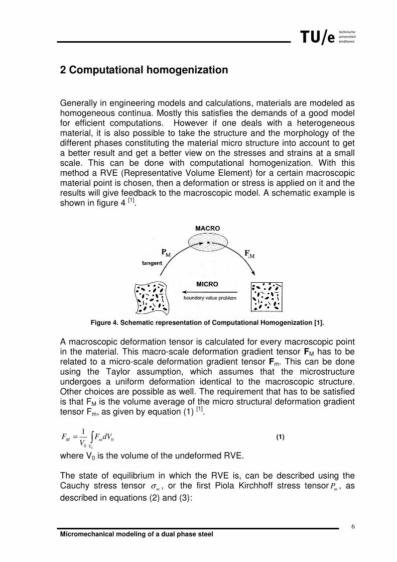
2 Computational homogenization Generally in engineering models and calculations, materials are modeled as homogeneous continua. Mostly this satisfies the demands of a good model for efficient computations. However if one deals with a heterogeneous material, it is also possible to take the structure and the morphology of the different phases constituting the material micro structure into account to get a better result and get a better view on the stresses and strains at a small scale. This can be done with computational homogenization. With this method a RVE (Representative Volume Element) for a certain macroscopic material point is chosen, then a deformation or stress is applied on it and the results will give feedback to the macroscopic model. A schematic example is shown in figure 4 [1].

Figure 4. Schematic representation of Computational Homogenization [1].

A macroscopic deformation tensor is calculated for every macroscopic point in the material. This macro-scale deformation gradient tensor FM has to be related to a micro-scale deformation gradient tensor Fm. This can be done using the Taylor assumption, which assumes that the microstructure undergoes a uniform deformation identical to the macroscopic structure. Other choices are possible as well. The requirement that has to be satisfied is that FM is the volume average of the micro structural deformation gradient tensor Fm, as given by equation (1) [1].

0

0

0

1M m

V

F F dVV

= ∫ (1)

where V0 is the volume of the undeformed RVE. The state of equilibrium in which the RVE is, can be described using the Cauchy stress tensor

mσ , or the first Piola Kirchhoff stress tensor

mP , as

described in equations (2) and (3):

13


0m m

σ∇ =�

i in V, (2)

Or:

00

c

m mP∇ =

�

i in V0, (3)

Where

m∇ is the gradient operator with respect to the current configuration

and 0m

∇ the gradient operator with respect to the undeformed configuration

of the micro structural cell.

With constitutive laws the mechanical behavior of the microstructure can be described. This law is formulated in a general form as follows [1]:

[ ]{ }( ) ( ) ( )( ) ( ), 0,

m mt F tα α α

σσ τ τ= ℑ ∈ (4)

Or as :

[ ]{ }( ) ( ) ( )( ) ( ), 0,

m P mP t F tα α α τ τ= ℑ ∈ (5)

Where t stands for the current time, 1, Nα = , with N the number of micro

structural constituents to be distinguished. With use of appropriate boundary conditions this problem can be solved. There are three kinds of boundary conditions, namely:

• Prescribed displacement

• Prescribed tractions

• Prescribed periodicity The prescribed tractions are not possible in combination with a deformation tensor since it is prescribed with use of stresses. For the calculations in this project the prescribed periodicity is used and will be further explained in the next chapter. From the solution of the boundary value problem, the macroscopic stress tensor, namely the first Piola Kirchhof stress tensor (PM), is calculated by averaging the resulting micro scale stresses (Pm) over the volume of the RVE. The obtained stress tensor can then be incorporated in the macroscopic model.

0

0

10 0

1 1 pN

PM m p

pV

P P dV f XV V =

= = ∑∫��

i (6)

with p

f��

the reaction forces on the nodes at which the displacements were

prescribed and PX��

the position vectors of these nodes.

13


2.1 Post-processing calculations

In the previous part all the calculations were needed to complete the computational homogenization, but in this work also the equivalent Cauchy stress is calculated out of the First Piola Kirchhoff stress tensor. They will be used for the post-processing and comparison of the different RVE’s responses. The calculations consist of different steps: Compute the Kirchhoff stress tensor [2]:

T

M M MP Fτ = i (7)

And the Cauchy stress tensor [2]:

1M M

MJ

σ τ= (8)

with ( )detM MJ F= the third invariant of M

F .

Finally we obtain the equivalent Cauchy stress as [2]:

, :T

M eq M Mσ σ σ= (9)

The stresses will be plotted as a function of the equivalent Green-Lagrange strain. This is calculated as follows [2]:

( )1

2

T

M M ME F F I= −i (10)

, :T

M eq M ME E E= (11)

Because the deformation is applied in several steps (increments) the deformation prescribed at each step is:

( )M

t

F IF I t

n

−= + ⋅ (12)

With t the current increment number and n the total number of increments.

13


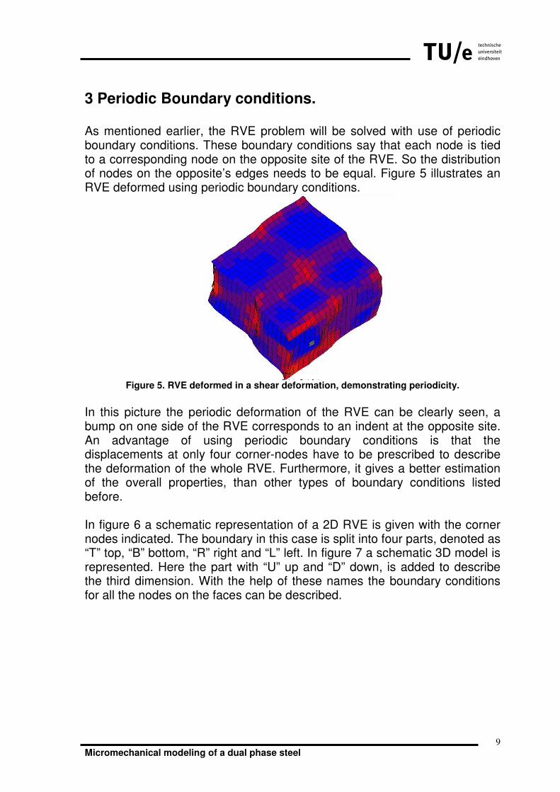
3 Periodic Boundary conditions. As mentioned earlier, the RVE problem will be solved with use of periodic boundary conditions. These boundary conditions say that each node is tied to a corresponding node on the opposite site of the RVE. So the distribution of nodes on the opposite’s edges needs to be equal. Figure 5 illustrates an RVE deformed using periodic boundary conditions.

Figure 5. RVE deformed in a shear deformation, demonstrating periodicity.

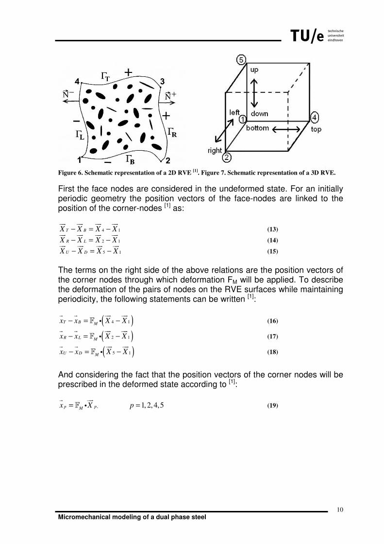
In this picture the periodic deformation of the RVE can be clearly seen, a bump on one side of the RVE corresponds to an indent at the opposite site. An advantage of using periodic boundary conditions is that the displacements at only four corner-nodes have to be prescribed to describe the deformation of the whole RVE. Furthermore, it gives a better estimation of the overall properties, than other types of boundary conditions listed before. In figure 6 a schematic representation of a 2D RVE is given with the corner nodes indicated. The boundary in this case is split into four parts, denoted as “T” top, “B” bottom, “R” right and “L” left. In figure 7 a schematic 3D model is represented. Here the part with “U” up and “D” down, is added to describe the third dimension. With the help of these names the boundary conditions for all the nodes on the faces can be described.

13


Figure 6 . Schematic representation of a 2D RVE

[1]. Figure 7. Schematic representation of a 3D RVE.

First the face nodes are considered in the undeformed state. For an initially periodic geometry the position vectors of the face-nodes are linked to the position of the corner-nodes [1] as:

4 1T BX X X X− = −��

(13)

2 1R LX X X X− = −��

(14)

5 1U DX X X X− = −��

(15) The terms on the right side of the above relations are the position vectors of the corner nodes through which deformation FM will be applied. To describe the deformation of the pairs of nodes on the RVE surfaces while maintaining periodicity, the following statements can be written [1]:

( )4 1T B Mx x X X− = −� � ��

iF (16)

( )2 1R L Mx x X X− = −� � ��

iF (17)

( )5 1U D Mx x X X− = −� � ��

iF (18)

And considering the fact that the position vectors of the corner nodes will be prescribed in the deformed state according to [1]:

,pp Mx X=� ��

iF 1, 2, 4,5p = (19)

13


The periodic boundary conditions (16)-(18) can be rewritten as [1]:

4 1T Bx x x x= + −� � � �

(20)

2 1R Lx x x x= + −� � � �

(21)

5 1U Dx x x x= + −� � � �

(22) Finally these position vectors can be written in terms of displacements and then implemented in a FEM package like MSC.Marc. These boundary conditions are then applied as tying relations between the nodes, in the MSC.Marc package called SERVO LINKS.

13


4 The Micromodel Computational homogenization is of course a good way to take the microstructure into account within the macro scale calculations. But in order to do that, a good micro model is needed. It has to represent all the properties of the material, without introducing non-existing properties. For example, when a RVE is large enough, the stress fields around small asymmetric particles will cancel each other and result in an overall isotropic behavior, but if one takes a RVE that is too small, an asymmetric particle will lead to anisotropy. So there are some requirements for a good RVE that are listed below:

• Must contain all microstructural properties

• Has to be large enough to realistically represent the microstructure and to exclude non-existing properties like anisotropy

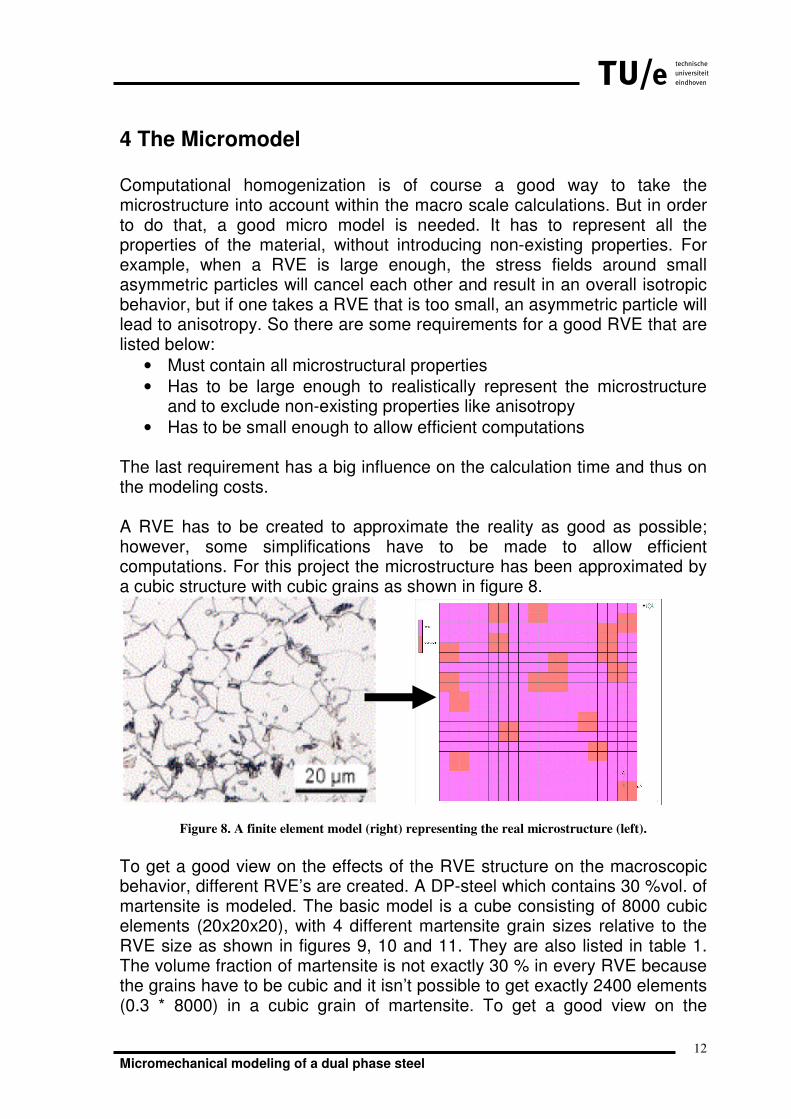
• Has to be small enough to allow efficient computations The last requirement has a big influence on the calculation time and thus on the modeling costs. A RVE has to be created to approximate the reality as good as possible; however, some simplifications have to be made to allow efficient computations. For this project the microstructure has been approximated by a cubic structure with cubic grains as shown in figure 8.

Figure 8. A finite element model (right) representing the real microstructure (left). To get a good view on the effects of the RVE structure on the macroscopic behavior, different RVE’s are created. A DP-steel which contains 30 %vol. of martensite is modeled. The basic model is a cube consisting of 8000 cubic elements (20x20x20), with 4 different martensite grain sizes relative to the RVE size as shown in figures 9, 10 and 11. They are also listed in table 1. The volume fraction of martensite is not exactly 30 % in every RVE because the grains have to be cubic and it isn’t possible to get exactly 2400 elements (0.3 * 8000) in a cubic grain of martensite. To get a good view on the

13


influence of the randomness of the microstructural distribution for every grain size, 5 random configurations are created. Table 1. Different RVE’s used

Side-length Number of martensite grains

Volume percentage of total

Grainsize 1 2400 grains 30%

Grainsize 2 300 grains 30%

Grainsize 5 19 grains 29.69%

Grainsize 13 1 grain 27,46%

Figure 9. Grain size 1. Figure 10. Grain size 5. Figure 11. Grain size 13.

13


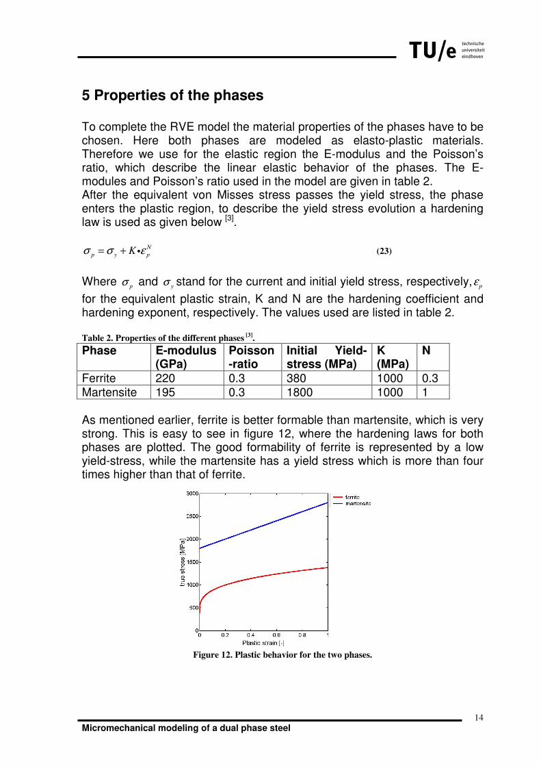
5 Properties of the phases To complete the RVE model the material properties of the phases have to be chosen. Here both phases are modeled as elasto-plastic materials. Therefore we use for the elastic region the E-modulus and the Poisson’s ratio, which describe the linear elastic behavior of the phases. The E-modules and Poisson’s ratio used in the model are given in table 2. After the equivalent von Misses stress passes the yield stress, the phase enters the plastic region, to describe the yield stress evolution a hardening law is used as given below [3].

N

p y pKσ σ ε= + i (23)

Where

pσ and

yσ stand for the current and initial yield stress, respectively, p

ε

for the equivalent plastic strain, K and N are the hardening coefficient and hardening exponent, respectively. The values used are listed in table 2. Table 2. Properties of the different phases

[3].

Phase E-modulus (GPa)

Poisson-ratio

Initial Yield-stress (MPa)

K (MPa)

N

Ferrite 220 0.3 380 1000 0.3 Martensite 195 0.3 1800 1000 1 As mentioned earlier, ferrite is better formable than martensite, which is very strong. This is easy to see in figure 12, where the hardening laws for both phases are plotted. The good formability of ferrite is represented by a low yield-stress, while the martensite has a yield stress which is more than four times higher than that of ferrite.

Figure 12. Plastic behavior for the two phases.

13


6 Results

6.1 Prescribed deformation modes

Three different types of deformation are chosen to investigate the behavior of the RVE’s. The deformations are set as shown in table 3, with the deformation gradient tensor given in the last column.

Table 3. The prescribed deformation modes

The selected tension deformation mode is accompanied by an increase in volume. Such deformation is not realistic; however it still can be investigated numerically. For the compression and shear the volume will stay constant.

6.2 Variation on randomness

As a first variable to be considered, the influence of the randomness of the microstructure is evaluated. For this the response of the five random configurations per grain size are compared using statistics. The deviation in the response of the different structures is evaluated using the following formulas:

Tension

1 1 2 2 3 311.1F e e e e e e= + +� � � � � �

Compression

1 1 2 2 3 32

1 10.9

0.9 0.9F e e e e e e= + +

� � � � � �

Simple Shear

1 1 1 2 2 2 3 330.1F e e e e e e e e= + + +

� � � � � � � �

13


Mean stress:

1

n

i

i

x

xn

==∑

(24)

Standard deviation:

( )2

1

1

n

i

i

x x

sn

=

−

=−

∑ (25)

With n the number of random configurations and xi the stress calculated on the random configuration i. For all different grain sizes the maximum deviation is obtained and the results are summarized in table 4. Here the relative deviation is shown which means that it is divided by the mean stress as given by equation (22), so it is possible to compare the different RVE’s or the different deformation modes.

100%r

ss

x= i (26)

Table 4. Relative deviation for random configurations per grain size and deformation mode.

Deformation\Size 1 2 5 13

tension 0.0075% 0.0039% 0.0182% 0.0027%

compression 0.1462% 0.2957% 1.2577% 0.0039%

shear 0.5088% 0.5182% 2.6833% 0.0013%

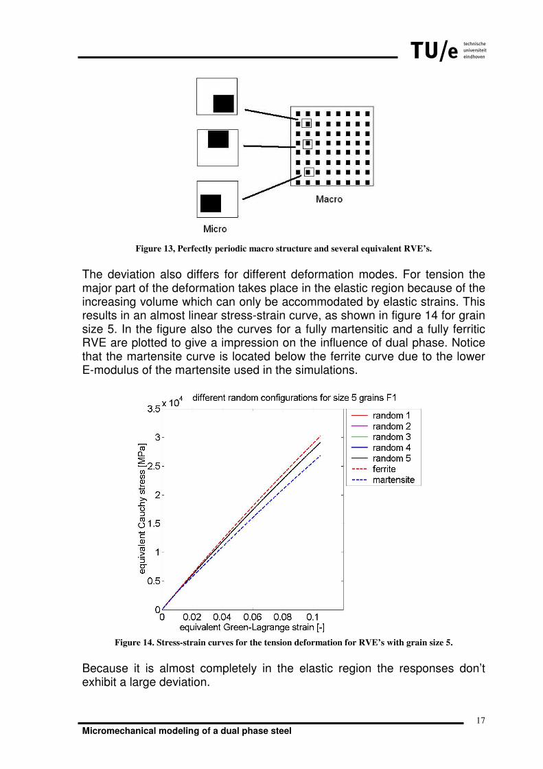
The influence of the randomness stays in general beneath one percent. Only for grain size 5 the influence rises to more than one percent which indicates an increase of the deviation for increasing grain size, although for grain size 13 the deviation never exceeds 0.005 percent. This can be explained by the perfect periodicity. Because there is only one martensite grain in a RVE the macroscopic configuration will be the same for any RVE irrespectively of the exact position of the grain in the RVE, as illustrated in figure 14.

13


Figure 13, Perfectly periodic macro structure and several equivalent RVE’s.

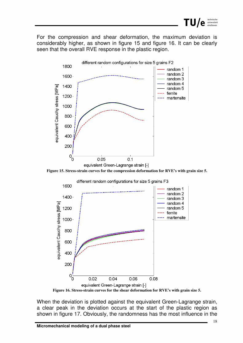
The deviation also differs for different deformation modes. For tension the major part of the deformation takes place in the elastic region because of the increasing volume which can only be accommodated by elastic strains. This results in an almost linear stress-strain curve, as shown in figure 14 for grain size 5. In the figure also the curves for a fully martensitic and a fully ferritic RVE are plotted to give a impression on the influence of dual phase. Notice that the martensite curve is located below the ferrite curve due to the lower E-modulus of the martensite used in the simulations.

Figure 14. Stress-strain curves for the tension deformation for RVE’s with grain size 5.

Because it is almost completely in the elastic region the responses don’t exhibit a large deviation.

13


For the compression and shear deformation, the maximum deviation is considerably higher, as shown in figure 15 and figure 16. It can be clearly seen that the overall RVE response in the plastic region.

Figure 15. Stress-strain curves for the compression deformation for RVE’s with grain size 5.

Figure 16. Stress-strain curves for the shear deformation for RVE’s with grain size 5.

When the deviation is plotted against the equivalent Green-Lagrange strain, a clear peak in the deviation occurs at the start of the plastic region as shown in figure 17. Obviously, the randomness has the most influence in the

13


plastic region and especially at the start of this region. Qualitatively similar results have been observed for other grain sizes.

Figure 17. Deviation of the random configurations for the different deformations for RVE’s with grain

size 5.

13


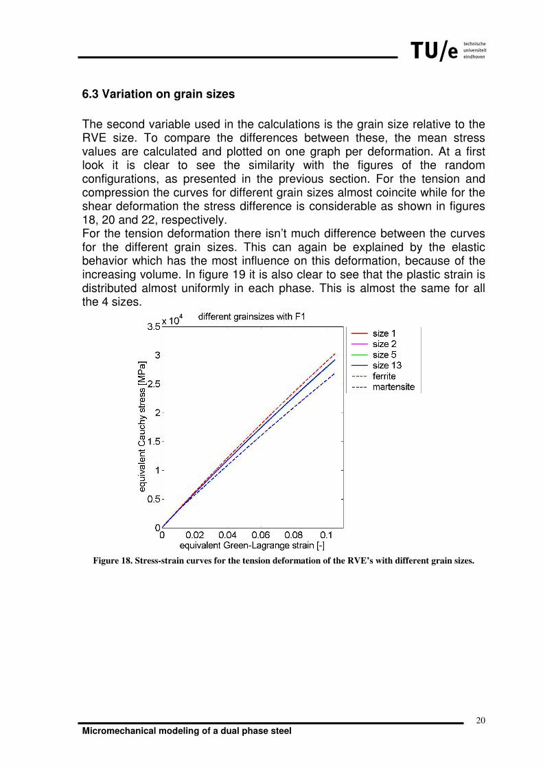
6.3 Variation on grain sizes

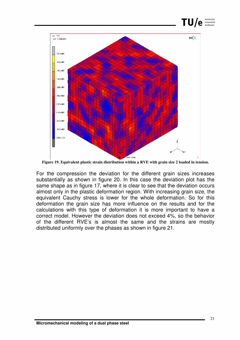
The second variable used in the calculations is the grain size relative to the RVE size. To compare the differences between these, the mean stress values are calculated and plotted on one graph per deformation. At a first look it is clear to see the similarity with the figures of the random configurations, as presented in the previous section. For the tension and compression the curves for different grain sizes almost coincite while for the shear deformation the stress difference is considerable as shown in figures 18, 20 and 22, respectively. For the tension deformation there isn’t much difference between the curves for the different grain sizes. This can again be explained by the elastic behavior which has the most influence on this deformation, because of the increasing volume. In figure 19 it is also clear to see that the plastic strain is distributed almost uniformly in each phase. This is almost the same for all the 4 sizes.

Figure 18. Stress-strain curves for the tension deformation of the RVE’s with different grain sizes.

13


Figure 19. Equivalent plastic strain distribution within a RVE with grain size 2 loaded in tension.

For the compression the deviation for the different grain sizes increases substantially as shown in figure 20. In this case the deviation plot has the same shape as in figure 17, where it is clear to see that the deviation occurs almost only in the plastic deformation region. With increasing grain size, the equivalent Cauchy stress is lower for the whole deformation. So for this deformation the grain size has more influence on the results and for the calculations with this type of deformation it is more important to have a correct model. However the deviation does not exceed 4%, so the behavior of the different RVE’s is almost the same and the strains are mostly distributed uniformly over the phases as shown in figure 21.

13


Figure 20. Stress-strain curves for the compression deformation of the RVE’s with different grain sizes.

Figure 21. Equivalent plastic strain distribution within a RVE with grain size 2 loaded in compression.

Although the stresses obtained under tension and compression have a relatively small deviation, the deviation for the shear deformation is about 11.5 %. The standard and relative standard deviations for cell deformation modes are listed in table 5.

13


It is again remarkable to see that the equivalent Cauchy stress lowers for increasing grain size as shown in figure 22. As shown in figures 9, 10 and 11, it is clear to see that the ferrite is less scattered for increasing grain size and because of its lower initial yield stress the ferrite can easily deform around the harder martensite grain. This leads to lower plastic strains in the martensite grains. In figure 23 it is also clear to see that for increasing grain size the plastic strain becomes more localized per phase. This occurs especially in the ferrite phase. For the shear deformation it can be concluded that it is very important to have a good representative RVE to get the correct modeling results.

Figure 22. Stress-strain curves for the shear deformation of the RVE’s with different grain sizes.

13


Figure 23. Equivalent plastic strain distribution within a RVE with grain size 2, 5 and 13

loaded in simple shear.

Table 5, standard and relative standard deviation of the RVE’s with different grain sizes.

Deformation Max-deviation[MPa]

Percentage of mean stress

Tension 41.2078 0.1492%

Pressure 25.8412 3.8990%

shear 74.0501 11.3776%

13


7 Conclusions From the literature study it has been concluded that the use of high performance steel will grow and that the computational homogenization is an important tool to create correct models. With the computational homogenization it is possible to take into account the structure and the morphology of the different phases constituting the material micro structure to obtain a better result and get a better view on the stresses and strains at a small scale. To use this technique there is a need for a good micro scale model. Several models, Representative Volume Elements (RVE) for a dual phase steel have been created in this work to test the influence of spatial randomness and the grain size (relative to the RVE size) of the martensite grains on the stress output. It follows that for the models considered the randomness per grain size does not have a great influence on the stress output, although the deviation increases slightly with increasing grain size. The results also show a larger deviation for the shear deformation in comparison to the tension and compression and especially at the start of plastic deformation. When the different grain sizes are compared it is also clear that for the tension and compression the deviations are not that high. But for the shear deformation the differences are significant. With increasing grain size, the overall equivalent Cauchy stress lowers. It is observed that the martensite grains show much less plastic deformation than the ferrite phase of the RVE. Therefore when computational homogenization is used to describe shear deformations, it is especially important to have a correct microstructure model. It can be concluded that in general choosing a RVE for a certain material is a delicate task which should be done with care.

13


8 Recommendations In this project the only considered microstructural variables were the grain size and the random spatial configuration. In practice, there exist of course a lot more variables; a few of them which can be taken into account in future research are listed below.

• Different grain sizes in one RVE.

• Random grain geometry (not only cubic).

• Influence of the phase volume fraction percentage. These are all measures to approach the real microstructure as much as possible. To compare the models with the real material some physical experiments have to be done to obtain the real material properties, so the best RVE can be obtained. The M-files (Matlab) developed in this project can also be used to create RVE’s for other materials. The files have different variables as listed below:

• RVE-size (number of elements).

• Grain size, relative to RVE size.

• Volume percentage of grains.

• Material properties. With the adaptation of these variables it is possible to create RVE’s for other high performance steels, like TRIP.

13


9 Bibliography [1] V.G. Kouznetsova, Computational Homogenization for the multi-scale

analysis of multi-phase materials, PhD thesis, Netherlands Institute for Metals Research, Department of Mechanical Engineering, Eindhoven University of Technology Eindhoven, The Netherlands, 2002.

[2] Continuum Mechanics for Manufacturing Technology, Lecture notes – course 4C600, M.G.D. Geers, F.P.T. Baaijens, P.J.G. Schreurs, Eindhoven University of Technology, Faculty of Mechanical Engineering, 2005.

[3] Spyros Papaefthymiou, Failure mechanisms of multiphase steels, PhD thesis, Fakultät für Georessourcen und Materialtechnik der RWTH Aachen, 2005.

[4] Frédéric Lani, Micro-mechanical modeling of dual-phase elasto-plastic materials, influence of the morphological anisotropy, continuity and transformation of the phases. PhD thesis, Faculte des Sciences Appliquees, Universite catholique de Louvain, 2005.

Documents

Micromechanical modeling of a dual phase steel · Micromechanical modeling of a dual phase steel 2 Abstract Dual Phase steel (DP-steel) is one of the more common advanced steels and