Copyright 0 1995 by the Genetics Society of America

An Evaluation of Genetic Distances for Use With Microsatellite Loci

David B. Goldstein, * Andres Ruiz bares, Luigi Luca Cavalli-Sforzaf and Marcus W. Feldman * *Department of Biological Sciences, Stanford University, Stanford, California 94305, Universidad de Antioquia,

Famltad de Medicina, Centro de Investigaciones Medicas, Medellin, Colombia and x Department of Genetics, Stanford University, Stanford, California 94305

Manuscript received June 22, 1994 Accepted for publication October 5 , 1994

ABSTRACT Mutations of alleles at microsatellite loci tend to result in alleles with repeat scores similar to those

of the alleles from which they were derived. Therefore the difference in repeat score between alleles carries information about the amount of time that has passed since they shared a common ancestral allele. This information is ignored by genetic distances based on the infinite alleles model. Here we develop a genetic distance based on the stepwise mutation model that includes allelic repeat score. We adapt earlier treatments of the stepwise mutation model to show analytically that the expectation of this distance is a linear function of time. We then use computer simulations to evaluate the overall reliability of this distance and to compare it with allele sharing and Nei’s distance. We find that no distance is uniformly superior for all purposes, but that for phylogenetic reconstruction of taxa that are sufficiently diverged, our new distance ispreferable.

S TUDIES of phylogenetic relationships among very closely related species are often hampered by a lack

of variation. For example, in their study of mitochon- drial DNA variation in the Lake Victoria flock of East African cichlids, MEYER et al. ( 1990) found no variation in a 363-bp region of the cytochrome b gene and an average of two or three substitutions separating species in 440 bp of the control region. The estimation of rela- tionships among such closely related taxa, or the estima- tion of relationships within a species, would be easier if faster evolving characters were used. Because of their exceptionally high mutation rate, microsatellites may prove more informative for working out relationships among such closely related species, as well as among subpopulations of a single species ( BOWCOCK et al. 1994).

Microsatellites are a special class of tandem repeat loci that involve a base motif of 1-6 bp repeated up to - 100 times ( TAUTZ 1993). The few tandem repeat loci that have been studied show exceptionally high muta- tion rates, with minimal rates as high as lo-’ (JEFFREY~ et al. 1988; KELLY et al. 1991 ) or 10 -‘ ( LEVINSON and GUTMAN 1987; HENDERSON and PETES 1992). Because of this and the generally large number of alleles avail- able, these loci have been extremely useful in DNA fingerprinting (JEFFREB and PENA 1993; QUELLER et al. 1993), linkage analysis (TODD et al. 1991; DIETRICH et al. 1992) and more recently in the reconstruction of human phylogeny ( BOWCOCK et al. 1994).

Although microsatellites may prove to be more useful

Cmesponding author: David B. Goldstein, Department of Biology, The Pennsylvania State University, 208 Mueller Laboratory, University Park, PA 16802-5301. E-mail: david@kimura.stanford.edu

Genetics 139: 46.51171 (January, 1995)

than classical polymorphisms (or sequence data) for assessing population structure and determining the re- lationships among very closely related species, they may be less informative for more distantly related taxa. This is because the range of variation in number of repeats, while large, is ultimately restricted (BOWCOCK et al. 1994). Therefore, after sufficient time has passed, any distance applied to these loci will reach a maximal value.

Although a large number of evolutionary distances could conceivably be applied to microsatellites (see be- low), there has been relatively little theoretical evalua- tion of inferences and their reliability (but see CHAKRA- BORTY and JIN 1993). Furthermore, alleles at some of these loci are thought to evolve by a stepwise mutation process, in which an allele mutates up or down by a small number of repeats ( SCHLOTTERER and TAUTZ 1992). Therefore, estimators of population parameters based on the infinite-alleles model, for example, are unlikely to apply to microsatellite loci. Although this stepwise mutation model is consistent with the distribu- tion of alleles at microsatellite loci ( SHRIVER et al. 1993; VALDES et al. 1993), it is probably not applicable to minisatellite loci ( SHRIVER et al. 1993). Furthermore, DI RIENZO et al. (1994) provide evidence that a strict (single-step) stepwise mutation model may not be suf- ficient to account for allele frequency distributions at microsatellite loci.

In this paper we first derive a distance measure that is linear with time when applied to loci undergoing a strict stepwise mutation process with no constraint on allele size and then use computer simulations to evalu- ate the reliability of this and other distances. We con-

464 D. B. Goldstein et al.

sider both the reliability of phylogenetic reconstruction and the reliability of inferences about the populations to which individuals belong.

A LINEAR GENETIC DISTANCE FOR MICROSATELLITES

Here we adapt earlier treatments of the stepwise mu- tation model to obtain an evolutionary distance whose expectation is linear with time. The reliability of an evolutionary distance depends both on its expectation and variance, but a linear expectation is desirable if it does not entail too large an increase in the variance. OHTA and KIMURA’S (1973) stepwise mutation model was originally applied to changes in the charge state of proteins as inferred from electrophoretic mobility. More detailed mathematical and statistical analyses of this model, including the possibility of two-step muta- tions, were made by MORAN ( 1975), WEHRHAHN (1975), BROWN et al. (1975), WEIR et al. (1976) and others.

We consider here only the strict stepwise mutation model, in which an allele with i repeats mutates to each of i - 1 and i + 1 repeats with probability p / 2 . Assume a population of N diploid individuals. MORAN ( 1975) showed that with multinomial sampling, the probability distribution of n, ( t ) , the number of gametes carrying an allele with i repeats at time t , does not converge as t grows large. Similarly, the mean number of repeats, ( 2 N ) X, ini ( t ) , does not converge (although the ex- pected value of this mean does not change with time). The variance in repeat number, given the initial condi- tions, however, does converge. Thus, although the aver- age of the number of repeats never reaches an equilib- rium value, the “cloud” around the mean retains constant variance as the mean position wanders. MORAN ( 1975 ) also showed that the random variables C, ( t ) = ( 2 N ) -‘ Z8 nj ( t ) nL+k( t ) converge. For example, E [ C,] approaches (1 + 28) where 8 = 4Np, a result also derived by OHTA and KIMURA (1973). Its reciprocal is the effective number of alleles.

If D,, is defined as the average squared difference in repeat numbers for two alleles drawn from the same population, then direct application of MORAN’S (1975) results yields the limiting expectation, E ( Do) = 2 (2N - 1 ) p. Similarly, define Dl as the average squared dif- ference in repeat numbers for two alleles drawn one each from different populations isolated T generations in the past. For convenience we will refer to a distance based on D, as the average squared distance. In the APPENDIX we show that the expectation of Dl is a linear function of T . Specifically,

E[D1 ( T ) ] = 2 ( 2 N - 1 ) p -t T ~ P . (1)

SLATKIN ( 1995) has also derived very similar expecta- tions using coalescent theory. He found that the aver-

age squared difference between alleles is ZpoiT, where t 1s the expected coalescence time between the alleles, p is the mutation rate and CT; is the variance of the distribution of mutations. Within a single population 7 is 2N (HUDSON 1990). This gives E ( Do) = 4Np for the strict stepwise mutation model. The expected coales- cence time for alleles drawn from each of two popula- tions separated T generations ago is 2N + T ( SLATKIN 1995), from which E ( D l ) may be derived. These results agree with those derived above upon substitution of 2N for 2N - 1. Note that Slatkin’s analysis allows mutations of more than one repeat unit in the stepwise mutation model.

- .

INFERENCES BASED ON VARIATION AT MICROSATELLITE LOCI

Estimation of D,: If it is known a pn‘ori to which population each individual belongs, the phylogenetic relationships among the populations can be inferred using an estimate of Dl based on the sampled individu- als. An obvious estimator of Dl can be written in terms of the repeat scores of two sampled alleles i, i’. Namely,

&, = ( i - i ’ ) 2 . ( 2 )

It is easy to see that the average (a) of A between all alleles sampled, one from each population, is an unbiased estimator of E [ Dl 3 . Denote E, as the expecta- tion under random sampling from the two populations, then the expectation of ( A ) is E,,[ A ] = E,\ E, C,, ( i - i ’ ) ‘ JJ , , where the sum is over all i , i ’ , andJ, J f are, respectively, the frequencies of alleles i and i’ in the samples from the first and the second population. Thus, because sampling is independent in the two popula- tions, we have &,[A] = X i C,, ( i - i ’ ) 2 E , [ J ] E , [ J f ] = Xi E,, ( i - i’) ‘F,Er = Dl where F, , FL, are, respectively, the parametric frequencies of alleles i and i’ in the first and second population. Therefore, is an unbiased estimator of D, . Thus, the expectation of A should be a linear function of the time since the populations were isolated.

Phylogeny reconstruction: We confirmed the linear- ity of Li using computer simulation and also compared its behavior with two other distances: allele sharing (D,4s), which has recently been used to infer human phylogenetic relationships ( BOWCOCK et al. 1994) , and Nei’s distance ( NEI 1972) , denoted In Figure 1 the mean behaviors of a, DAS and DS are compared. The figure reports the results of 100 independent simula- tions, all using the same parameters ( N , p ) . For conve- nience we will refer to the generation time in compar- ing the behavior of the distances, but it should be noted that such references are specific to the particular values of N and p used in the simulation. Notice that after sufficient time has passed (here about 1000 genera- tions), both DAs and D,s are beginning to asymptote,

Microsatellite Genetic Distances 465

A 6 7 1

5

4

a

c :3 m 0 -

2

1

0

Generations

C

0.8

0.7

0.6 u C a I - m 0.5 0

0.4

0.3

0.2 ! I .

0 500 1000 1500 2000 2500 Generatlons

- . 0 500 1000 1500

Generations

2000

0.54 f

5 0.3 c

Nei’s Distance I E 0.2

0.1 1-1 Allele Sharing I

0.0 ! 1 I I I ’

0 500 1000 1500 2000 2500 Generations

FIGURE 1.-Means and variances of the distances as a function of time. To determine the mean of the distance estimates as a function of time, we started with two identical populations with an equilibrium variance of repeat number. This equilibrium was reached by iteration. We simulated the independent evolution of these populations for 2500 generations. The haploid population size of each taxon was 200 and an allele in state i mutated to state i + 1 and i - 1 with probability 0.0005 each psr generation. The next generation was formed by random sampling of the previous generation. We calculated each distance (A , DAs, DS) every 100 generations. D,4.y was calculated based directly on the haploid populations as 1 - (the average number of shared alleles). That is, DAs = 1 - (1/2N) -‘ Z, Z: I( i, 2 ’ ) , where the first and second sums are over all alleles in the first and second population, and I ( i, i ‘ ) is an indicator variable that equals 1 if the alleles are the same and zero if they are not. The formula for A is given in the text, and the fcrmula for D,s (Nei’s “standard” distance) can be found in NEI ( 1972). Figure 1, A-C show, respectively, the average values of A, D,s and DAs among 100 independent simulations. Figure 1D shows the coefficients of variation for the three measures.

but A remains linear. A log transformation of DAs im- proves its linearity only slightly, making it similar to D,l.. Thus, we will not consider this further here.

Because the variance of an estimator also influences its performance, we estimated the coefficients of varia- tion of the distances (Figure ID) . Notice that the coef- ficient of variation of DA.5 is always smaller than that of

and D,$. Thus, DA,yis the superior distance with respect

to variance but inferior with respect to expectation. One criterion that can be used to determine which distance is superior is to compare the slope of the mean to the standard deviation at each point in time ( TAJIMA and TAKEZM 1994). This shows that A is superior after - 100 generations (data not shown) . Trees that include more distantly related taxa, therefore, should tend to be more accurately reconstructed by A.

466 D. B. Goldstein et al.

0 !!

I-

O

250 c

L W , . , . , . , . , ~ ,

0 1000 2000 3000 4000 5000 Length of Tree (Generatlons)

FIGURE 2.-Reliability of the distances in recovering the correct phylogeny. To test how the two distance measures influence the reliability of phylogenetic reconstruction, we simulated the stepwise mutation process along a three-taxon tree of variable length and inferred the phylogenetic relation- ship among the taxa at the end of the simulation using the UPGMA algorithm with each distance estimate. The total length of the tree varied from 50 to 4400 generations, the haploid population size of each taxon was 200, and the num- ber of loci was 15. The single speciation event occurred at the exact midpoint of the tree. We ran 400 independent simu- lations along each of the trees. The curves represent the num- ber of times out of 400 that the correct topology was inferred.

It is important to determine the expected difference in performance between DA,y and for different types of trees. We compared the overall reliability of DAS and A by simulating evolution along a three-taxon tree of variable length. Figure 2 shows that for trees of a total length shorter than -300 generations, DAs reconstructs phylogenies more accurately than A. From -500 gener- ations on, however, A is progressively more reliable than DAS.

Note from Equation 1 that, except for a constant factor independent of time, A is not a function of the population size. Therefore, unlike distances such as FsT

that measure the differentiation caused by sampling and not mutation, the appropriate measure of time for A is p r , not Nr.

Revealing cryptic population structure: For some data sets it may not be possible to determine member- ship of individuals in populations before genetic analy- sis is carried out. For example, we might be interested in testing whether a population that is not obviously partitioned into isolated subgroups is in fact genetically structured because of behavior (e.g., BOWEN et al. 1993) or because of recent admixture among a set of pre- viously distinct populations (e.g., BOWCOCK et al. 1994) .

When the proper assignment of individuals to popu- lations is not known, the mean squared differences among alleles in pairs of individuals can be split into

two components, giving information about D, and Do. Let the alleles in one individual be i l , i2 and those in the other be jl , j 2 . The total squared difference among the four alleles in these two individuals is V,. = 2 ( i l - i ~ ) ~ + 2 ( j 1 - j 2 ) ' + ( j 1 + j 2 - il - i2)'. The within- and between-individual components of this sum of squares are ( i l - i 2 ) 2 + (jl - j 2 ) ' and ( i , - j l ) 2 + ( i , - j 2 ) * + ( 2 2 - j , ) + ( i2 - j ,) ', respectively. The within-individual component is an estimate of Do (al- though not unbiased), because alleles within an indi- vidual must come from the same population (ignoring admixture) . At a single locus there is a total of N (total population size) observations that can be used to esti- mate Do. These may not all estimate the same value of Do, however, because the different subpopulations may have different population sizes.

The between-individual component of the sum of squares will reflect either Do or D l , depending on whether the two individuals come from the same or different populations. A matrix of these between-indi- vidual squared differences, therefore, will have ele- ments each of which is an estimate of either Do or Dl. If these estimates are sufficiently different, a clustering program will group individuals into their correct popu- lations. This is the basis for the approach taken by Bow- COCK et al. (1994), who used a distance measure based on the proportion of shared alleles between individuals (see also STEPHENS et al. 1992; CHAKRABORTY and JIN

1993). They found that trees of individuals based on this distance are structured into taxonomic units that correspond well with the geographic origins of the indi- viduals. This suggests that microsatellite loci can be used to assign individuals to the populations from which they come.

We simulated evolution on a three-taxon tree to de- termine whether & or DAS more accurately assigns indi- viduals to their correct populations. Figure 3 shows that over all trees evaluated DAS makes this assignment more accurately. Because A is more accurate over long peri- ods of time, this is at first puzzling. A possible explana- tion may involve the method of assignment of individu- als to populations. Denote by Dw, the expected value of either distance for two individuals drawn from the same population and by DB, the same for individuals drawn from different populations. ( I f there are more than two subpopulations there will be a series of D i s , one for each pair of populations.) For the individuals to be placed into taxonomic groups corresponding to the populations from which they come, it is necessary and sufficient that Dn be distinguishable from Dw It is not necessary that any of the different values of DR (representing individuals drawn from different pairs of populations) be distinguishable. Therefore, the fact that DAS asymptotes more quickly than Dl does not inter- fere with the assignment of individuals to populations, and its greater precision (lower variance) makes it the

Microsatellite Genetic Distances 467

0 l o o 200 300 400 500 600

Length of Tree (Generations)

FIGURE 3.-Reliability of assignment of individuals to popu- lations. To test how well and allele sharing assign individu- als to populations, we simulated evolution along a three-taxon tree as described above but with 75 haploid individuals of each taxon. The trees ranged in length from 100 to 600 gener- ations, and 100 replications were run for each tree length. At the end of the simulation, we assumed that the assignment of indiziduais to populations was unknown. We then used either A or allele sharing (see text) to build a tree of individu- als. The structure of this tree was then studied, and the aver- age number of individuals incorrectly assigned (out of 225) among the 100 replications was calculated.

superior distance for this purpose. Of course, the ar- rangement of the populations that results from DAs may be incorrect, but individuals coming from the same population will tend to cluster near one another regard- less of the arrangement of the populations within the tree.

PRACTICAL CONSIDERATIONS

Constraints on the maximum number of re- peats: The treatment above assumed that alleles can mutate to arbitrarily large or small repeat scores. In reality the number of possible repeat scores is restricted, and several lines of evidence suggest that this limit is fairly strict. BOWCOCK et al. (1994) found that the vari- ance in repeat score is approximately the same within humans and within primates. If there were no restric- tion, one would expect the greater evolutionary dis- tance among primates to lead to much greater differ- ences in repeat scores. Additionally, of the 20 loci typed in humans and the 10 also typed in the other primates (unpublished data), all but one has a maximal repeat score under 100. The demonstrated connection be- tween large repeat scores and hypermutability ( KUNKEL 1993; STRAND et al. 1993) suggests a mechanism for the constraint on repeat score.

The length of time during which Dl is (approxi-

mately) linear as a function of the maximum number of alleles possible, R (which is also the range of the repeat score ) , can be approximated as follows. Assume that each of two isolated populations has only one type of allele. Then, it is possible to calculate the average value of Dl after the isolated populations have reached maximal divergence. In this case the repeat score of the single allele in each population is randomly drawn from the possible R values. Therefore, the joint proba- bility distribution for the process of sampling an allele in state i from one population and an allele in state j from the other population is given by p ( i, j ) = 1 / R'. The maximum divergence possible as a function of R, denoted 6 ( R ) , is the expectation of ( i - j ) and is given by

Substituting 6( R ) for Dl ( t ) in Equation 1 and solving for T yields the amount of time it takes Dl to reach the value it takes at maximal divergence. This time should approximate the duration of linearity of Dl and is given bY

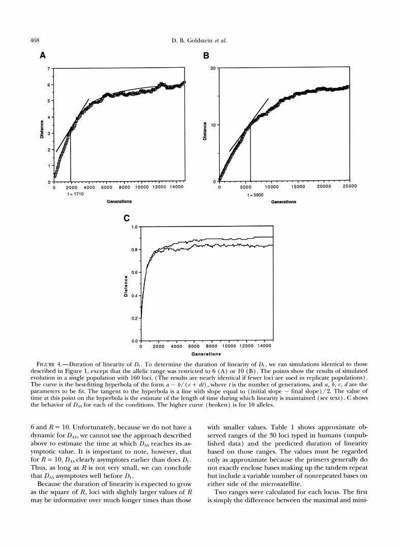
Figure 4 shows the results of computer simulations similar to those shown in Figure 1, except that the total number of alleles possible is restricted to 6 (Figure 4 A ) and 10 (Figure 4B). First, note that asymptotes at -6 and 17 for the respective simulations. This com- pares nicely with predictions of 19( 6) = 5.8 and 6( 10) = 16.3. Thus, the approximation for the maximum value of Dl given in Equation 3 appears to be quite accurate under these conditions.

In Figure 4 a hyperbolic function has been fitted to the simulation results. We take the point at which lin- earity is lost to be that point on the hyperbola where a tangent has slope halfway between the initial slope (based on Equation 1 ) and the final value (zero) . This method produces estimates of 1710 and 5900 for the approximate times that the simulated values of stopped their linear increase with time, somewhat lower than predicted by Equation 4 (2800 and 8100, respec- tively). This is probably due to the fact that the simula- tion reports the average values of a nonlinear function, from which we wish to infer the value of its argument (time). Because the average value of a nonlinear func- tion is not the same as the function applied to the average of its argument, the method used in Figure 4 provides a biased estimate of the time at which the slope is halfway between its initial and final values. Nonethe- less, it appears that Equation 4 provides a useful approx- imation of the range of linearity of D l . For comparison, Figure 4C shows the dynamic behavior of DAS for R =

D. B. Goldstein et nl. 468

A

t = 1710

Generations

C

B 20

4 10

- Q n

0

t = 5900 GeneraUons

0.0 0 2000 4000 6000 8000 10000 12000 14000

Generation8

FIGURE 4.-Duration of linearity of Dl. To determine the duration of linearity of D, , we ran simulations identical to those described in Figure 1 , except that the allelic range was restricted to 6 ( A ) or 10 ( B ) . The points show the results of simulated evolution in a single population with 160 loci. (The results are nearly identical if fewer loci are used in replicate populations). The curve is the best-fitting hyperbola of the form a - b/ ( c + d t ) , where 1 is the number of generations, and a, b, 6, dare the parameters to be fit. The tangent to the hyperbola is a line with slope equal to (initial slope - final slope) /2 . The value of time at this point on the hyperbola is the estimate of the length of time during which linearity is maintained (see text). C shows the behavior of D,,% for each of the conditions. The higher curve (broken) is for 10 alleles.

6 and R = 10. Unfortunately, because we do not have a dynamic for DAs, we cannot use the approach described above to estimate the time at which DAS reaches its as- ymptotic value. It is important to note, however, that for R = 10, DAs clearly asymptotes earlier than does D l . Thus, as long as R is not very small, we can conclude that DAS asymptotes well before Dl.

Because the duration of linearity is expected to grow as the square of R , loci with slightly larger values of R may be informative over much longer times than those

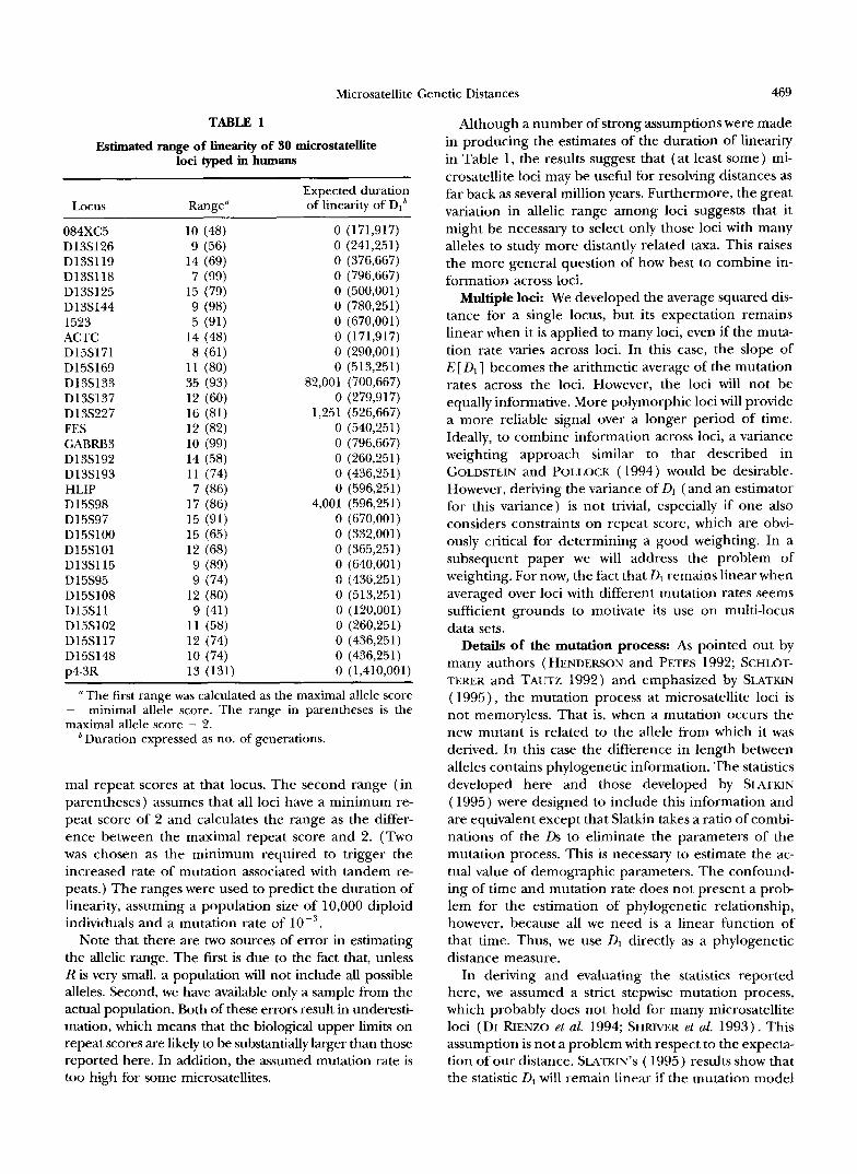
with smaller values. Table 1 shows approximate ob- served ranges of the 30 loci typed in humans (unpub- lished data) and the predicted duration of linearity based on those ranges. The values must be regarded only as approximate because the primers generally do not exactly enclose bases making up the tandem repeat but include a variable number of nonrepeated bases on either side of the microsatellite.

Two ranges were calculated for each locus. The first is simply the difference between the maximal and mini-

Microsatellite Genetic Distances 469

TABLE 1

Estimated range of linearity of 30 microstatellite loci typed in humans

Expected duration Locus Range" of linearity of Dlb

084XC5 10 (48) 0 (171,917) D13S126 9 (56) 0 (241,251) D13S119 14 (69) 0 (376,667) D13S118 7 (99) 0 (796,667) D13S125 15 (79) 0 (500,001) D13S144 9 (98) 0 (780,251) 1523 5 (91) 0 (670,001) ACTC 14 (48) 0 (171,917) D15S171 8 (61) 0 (290,001) D15S169 11 (80) 0 (513,251) Dl 3S133 35 (93) 82,001 (700,667) D13S137 12 (60) 0 (279,917) D13S227 16 (81) 1,251 (526,667) FES 12 (82) 0 (540,251) GABRB3 10 (99) 0 (796,667) D13S192 14 (58) 0 (260,251) D13S193 11 (74) 0 (436,251) HLIP 7 (86) 0 (596,251) D 15S98 17 (86) 4,001 (596,251) D15S97 15 (91) 0 (670,001) D15S100 15 (65) 0 (332,001) D15S101 12 (68) 0 (365,251) D13S115 9 (89) 0 (640,001) D 15S95 9 (74) 0 (436,251) D15S108 12 (80) 0 (513,251) D15Sll 9 (41) 0 (120,001) D15S102 11 (58) 0 (260,251) D15S117 12 (74) 0 (436,251) D15S148 10 (74) 0 (436,251) p43R 13 (131) 0 (1,410,001)

" The first range was calculated as the maximal allele score - minimal allele score. The range in parentheses is the maximal allele score - 2. ' Duration expressed as no. of generations.

mal repeat scores at that locus. The second range (in parentheses) assumes that all loci have a minimum re- peat score of 2 and calculates the range as the differ- ence between the maximal repeat score and 2. (Two was chosen as the minimum required to trigger the increased rate of mutation associated with tandem re- peats.) The ranges were used to predict the duration of linearity, assuming a population size of 10,000 diploid individuals and a mutation rate of

Note that there are two sources of error in estimating the allelic range. The first is due to the fact that, unless R is very small, a population will not include all possible alleles. Second, we have available only a sample from the actual population. Both of these errors result in underesti- mation, which means that the biological upper limits on repeat scores are likely to be substantially larger than those reported here. In addition, the assumed mutation rate is too high for some microsatellites.

Although a number of strong assumptions were made in producing the estimates of the duration of linearity in Table 1, the results suggest that (at least some) mi- crosatellite loci may be useful for resolving distances as far back as several million years. Furthermore, the great variation in allelic range among loci suggests that it might be necessary to select only those loci with many alleles to study more distantly related taxa. This raises the more general question of how best to combine in- formation across loci.

Multiple loci: We developed the average squared dis- tance for a single locus, but its expectation remains linear when it is applied to many loci, even if the muta- tion rate varies across loci. In this case, the slope of E [ Dl ] becomes the arithmetic average of the mutation rates across the loci. However, the loci will not be equally informative. More polymorphic loci will provide a more reliable signal over a longer period of time. Ideally, to combine information across loci, a variance weighting approach similar to that described in GOLDSTEIN and POLLOCK (1994) would be desirable. However, deriving the variance of Dl (and an estimator for this variance) is not trivial, especially if one also considers constraints on repeat score, which are obvi- ously critical for determining a good weighting. In a subsequent paper we will address the problem of weighting. For now, the fact that Dl remains linear when averaged over loci with different mutation rates seems sufficient grounds to motivate its use on multi-locus data sets.

Details of the mutation process: As pointed out by many authors (HENDERSON and PETES 1992; SCHLOT- TERER and TAUTZ 1992) and emphasized by SLATIUN (1995), the mutation process at microsatellite loci is not memoryless. That is, when a mutation occurs the new mutant is related to the allele from which it was derived. In this case the difference in length between alleles contains phylogenetic information. The statistics developed here and those developed by SLATKIN ( 1995) were designed to include this information and are equivalent except that Slatkin takes a ratio of combi- nations of the Ds to eliminate the parameters of the mutation process. This is necessary to estimate the ac- tual value of demographic parameters. The confound- ing of time and mutation rate does not present a prob- lem for the estimation of phylogenetic relationship, however, because all we need is a linear function of that time. Thus, we use D, directly as a phylogenetic distance measure.

In deriving and evaluating the statistics reported here, we assumed a strict stepwise mutation process, which probably does not hold for many microsatellite loci ( DI RIENZO et al. 1994; SHRIVER et al. 1993). This assumption is not a problem with respect to the expecta- tion of our distance. SLATKIN'S (1995) results show that the statistic Dl will remain linear if the mutation model

470 D. B. Goldstein et al.

is relaxed to include mutations of larger effect. Instead of a distance measure with slope p, where p is the aver- age mutation rateacross loci, the distance measure would have slope pa:. However, the variances of Dl, DAs and DSwill depend on the exact details of the muta- tion process, and the relative performance of the dis- tances will therefore depend on those details.

In fact, it is clear that the average squared distance will do progressively worse as the mutation model be- comes more like the infinite alleles model. Under the infinite-alleles model, we know that Nei's distance is linear and that the average square includes information that is not related to time since common ancestry (al- lelic repeat score) . Thus, the average square must be noisier and will perform worse. For a mixed model, we can assume that as the proportion of single-step mutations is reduced (and the proportion of arbitrary size goes u p ) , the performance of the average square relative to Nei's distance will decline.

A potentially more serious complication is that the mutation process may depend on the repeat score. If this dependence were strong, the results reported here would not be relevant. In particular, it might be inap- propriate to consider a repeat score of 2 as a reflecting boundary (WALSH 1987), and, more generally, if the mutation rate depends on the repeat score, Dl may not be linear.

We thank J. EISEN, J. KUMM, D. POLLOCK, M. SLATKIN and an anony- mous reviewer for helpful discussions and/or comments on earlier versions of this manuscript. This research was supported in part by National Institutes of Health grants GM-28016 to M.W.F., GM-20467 to L.C.S. and GM-28428 to L.C.S. and M.W.F. A.R.L. was supported in part by Colciencias and the Programa de Reproduccion, Universi- dad de Antioquia. A program that calculates various distances for microsatellites is available from Dr. Eric Minch, Department of Genet- ics, Stanford University. E-mail: Eric@Lotka.Stanford.edu

LITERATURE CITED

BOWCOCK, A. M., A. RUIZ-LINARES, J. TOMFOHRDE, E. MINCH, J. R. KIDD et al., 1994 High resolution of human evolutionary trees with polymorphic microsatellites. Nature 368: 455-457.

BOWEN, B. W., J. I . RICHARDSON, A. B. MEW, D. MARGARITOULIS, R. HOPKINS MURFWV and J. C. AVISE, 1993 Population structure of loggerhead turtles ( Curetta curetta) in the northwestern Atlan- tic Ocean and Mediterranean Sea. Consew. Biol. 7: 834-844.

BROWN, A. H. D., D. R. MARSHALI. and L. ALBERCH, 1975 Profiles of electrophoretic alleles in natural populations. Genet. Res. 25: 137-143.

CHAKRABORTY, R., and L. JIN, 1993 A unified approach to study hypervariable polymorphisms: statistical considerations of de- termining relatedness and population distances, pp. 153-175 in DNA Fingetpnnting: State ofthe Science, edited by S. D. J. PENA, R. CHAKRABORTY, J. T. EPPI.F.N and A. J. JEFFREI~. Birkhauser Verlag:

DIETRICH, W., H. KATZ, S. E. LINCOLN, H.S. SHIN, J. FRIEDMAN et Basel.

nl., 1992 A genetic map of the mouse suitable for intraspecific crosses. Genetics 131: 423-447.

DI RIENZO, A,, A. C. PETERSON, J. C. GARZ.4, A. M. VALDES, M. SLATKIN rt ab, 1994 Mutational processes of simple sequence repeat loci in human populations. Proc. Natl. Acad. Sci. USA 91: 3166- 3170.

GOLDSTEIN, D. B., and D. D. POLI.OCK, 1994 L,east squares estima-

tion of molecular distance-noise abatement in phylogenetic reconstruction. Theor. Popul. Biol. 45: 219-226.

HENDERSON, S. T., and T. D. PETES, 1992 Instability of simple se- quence DNA in Saccharomyces cerevisiae. Mol. Cell. Biol. 12: 2749- 2757.

HUDSON, R. R., 1990 Gene genealogies and the coalescent process. Oxf. Sum. Evol. Biol. 7: 1-44.

JEFFREYS, A.J . , and S. D. J. PENA, 1993 Brief introduction to human DNA fingerprinting, pp. 1-20 in DNA Fzngerpn'nting: State of the Science, edited by S. D. J. PENA, R. CHAKRABORTY, J. T. EPPIXN and A. .J. JEFFWE. Birkhauser Verlag: Basel.

JEFFREYS, A. J., N. J. ROYLE, V. WILSON and Z. WONG, 1988 Spontane- ous mutation rates to new length alleles at tandem-repetitive hypervariable loci in human DNA. Nature 322: 278-281.

KEI.I.Y, R., M. GIBBS, A. COLLICK and A. J. JEFFREE, 1991 Spontane- ous mutation at the hypervariable mouse minisatellites locus Ms6 hm: flanking DNA sequence and analysis of germline and early somatic events. Proc. R. SOC. Lond. Ser. B 245: 235-245.

KUNKEL, T. A,, 1993 Slippery DNA and diseases. Nature 365: 207-

LEVINSON, G., and G. A. GUTMAN, 1987 Slipped-strand mispairing: a major mechanism for DNA sequence evolution. Mol. Biol. Evol. 4 203-221.

MEYF.R, A., T. D. KOCHER, P. BASASIBWAKI and A. C. WIISON, 1990 Monophyletic origin of Lake Victoria cichlid fishes suggested by mitochondrial DNA sequences. Nature 347: 550-553.

MORAN, P. A. P., 1975 Wandering distributions and the electropho- retic profile. Theor. Popul. Biol. 8 318-330.

NEI, M., 1972 Genetic distance between populations. Am. Nat. 106:

OHTA, T., and K. KIMURA, 1973 The model of mutation appropriate to estimate the number of electrophoretically detectable alleles in a genetic population. Genet. Res. 22: 201-204.

QUEI.I.ER, D. C., J. E. STRLSSMANN and R. H. COLIN, 1993 Microsatel- lites and kinship. Tree 8: 285-288.

SCHL~TTERER, C., and D. TAUTZ, 1992 Slippage synthesis of simple sequence DNA. Nucleic Acids Res. 20: 211-215.

SHRIVER, M. D., L. JIN, R. CHAKRABORTY and E. BOERWINKLE, 1993 VNTR allele frequency distributions under the stepwise mutation model: a computer simulation approach. Genetics 134 983-993.

SIATKIN, M., 1995 A measure of population subdivision based on microsatellite allele frequencies. Genetics 139: 457-462.

STEPHENS, J. C., D. A. GILBERT, N. YUHKI and S. J. O'BRIEN, 1992 Estimation of heterozygosity for single-probe multilocus DNA fingerprints. Mol. Biol. Evol. 9: 729-743.

STRAND, M.,T.A. PROLW, R. M. LISKAYandT. D. PETES, 1993 Destabi- lization of tracts of simple repetitive DNA in yeast by mutations affecting DNA mismatch repair. Nature 365: 274-276.

TAJIMA, F., and N. TAKEZAKI, 1994 Estimation of evolutionary dis- tance for reconstructing molecular phylogenetic trees. Mol. Biol.

TAUTZ, D., 1993 Notes on the defunction and nomenclature of tan- demly repetitive DNA sequences, pp. 21-28 i n DNA Fzngerpn'nl- ing: State of the Science, edited by S. D. J. PENA, R. CHAKRABORTY, J. T. EPPIEN and A. J. JEFFWAS. Birkhauser Verlag: Basel.

TODD, J. A,, T. .J. AITMAN, R. J. CC)RNAI.I., S. GHOSH,J. R. s. HAIL et al., 1991 Genetic analysis of autoimmune type 1 diabetes melli- tus in mice. Nature 351: 542-547.

VAI.IXS, A. M., M. SIATKIN and N. B. FRFJMER, 1993 Allele frequen- cies at microsatellite loci: the stepwise mutatin model revisited. Genetics 133: 737-749.

WALSH, J. B., 1987 Persistence of tandem arrays: implications for satellite and simple-sequence DNAs. Genetics 115: 553-567.

WEHRHAHN, C., 1975 The evolution of selectively similar electropho- retically detectable alleles in finite natural popdatiOnS. Genetics 80: 375-394.

WEIR, B. S., A. H. D. BROWN and D. R. MARSHAIL, 1976 Testing for selective neutrality of electrophoretically detectable protein polymorphisms. Genetics 84: 639-659.

208.

283-292.

Evol. 11: 278-286.

Communicating editor: W. J. EWENS

Microsatellite Genetic Distances 47 1

APPENDIX

To derive the expectation of Dl as a function of time, define Eg as the single generation expectation operator. Then write

E,[Dl( t ) 1 = (2N)- 'Eg[C ( i - i ' ) 2 n i ( t ) n i , ( t ) ] , ( A l )

where the prime indicates the second population, and the sum is over all i, i'. Following MORAN (1975) , de- note ( 2 N ) -' Xi in, ( t ) as MI ( t ) and ( 2 N ) -' X, i'ni ( t ) as M2 ( t ) . Then, add and subtract squared means to get,

Eg[Dl ( t ) l = E g [ M z ( t ) - Ml(t)'I

+ Eg[M;( t ) - M ; ( t ) ' ] - 2(2N)- 'Eg

X [ ii'nt ( t ) n: ( t ) ] + EgMl ( t ) ' + EgMI ( t ) ' (A2)

= E g [ V ( t ) + V ' ( t ) ]

+ Eg[(M'(t) - W ( t ) ) ' I , (A3)

where V ( t ) is the variance in allelic repeat number at time t . Then substitute MOW'S (1975) equations for the sampling and mutation process (his Equations 6 and 7 ) to get

E,[D1( t ) ] = (1 - iN)(M,(t- 1) - M,(t- 1 ) 2 )

+ (1 - ; N ) p + (1 -iN)(M;(t- 1)

- M I 2 ( t - 1 ) ) + (1 - ; N ) p + (1 - iN)M1

1 x ( t - 1 ) 2 + - n/r , ( t - 1) + - P 2N 2N

+ (1 - i N ) M ; ( t - 1 ) * + - M ; ( t - 1 ) 1

2N

+" 2 M 1 ( t - l ) M ; ( t - 1 ) . (A4) P 2N

Rewriting in terms of the variances in the previous generation, we have E g [ D 1 ( t ) ] = ( 1 - i N ) ( V ( t - 1) + V ' ( t - 1 ) )

+ 2 ( 1 - 4 N ) p + ( 1 - t N ) M l ( t - 1 ) '

+ - - 2 M , ( t - l ) M i ( t - l ) , (A5) CL 2N

which simplifies to E g [ D 1 ( t ) ] = V ' ( t - 1) + V ( t - 1 )

+ 2p + M,(t- l ) ' + M f ( t - 1 ) 2

- 2 M 1 ( t - l ) M ; ( t - 1 ) . (A6) Then, noting that Dl ( t - I ) = V ( t - 1) + V ' ( t - 1 ) + (Ml(t- 1) - M ; ( t - l ) ) ' , w e have

E,[ Dl ( t ) 3 = Dl ( t - 1 ) + 2p. (A7 1 Now, define E as expectation over multiple generations. Then, the average squared difference between alleles drawn from populations isolated T generations ago is given by

E [ D l ( t ) ] = D o ( 0 ) + 72p. (A8 1 Assuming the population was at equilibrium when sepa- ration occurred, we have,

E [ D , ( t ) ] = 2 ( 2 N - 1 ) ~ + 72p. (A9)