Embed Size (px)
Citation preview

Introduction Methods K-means Spectral Clustering Markov Random Fields Modeling Data Mixture Modeling Conclusion
MicroscopySupervised Segmentation of Domain Boundaries in STM Images
of Self-Assembled Molecule Layers
Daniel Lander, Rodrigo Rios, Matt Vollmer, Yu (Dan) ZhouSupervised by: Dominique Zosso
Department of Mathematics, University of California, Los Angeles (UCLA)
08/07/2013
Introduction Methods K-means Spectral Clustering Markov Random Fields Modeling Data Mixture Modeling Conclusion
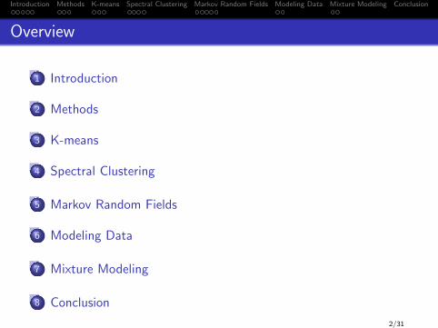
Overview
1 Introduction
2 Methods
3 K-means
4 Spectral Clustering
5 Markov Random Fields
6 Modeling Data
7 Mixture Modeling
8 Conclusion
2/31
Introduction Methods K-means Spectral Clustering Markov Random Fields Modeling Data Mixture Modeling Conclusion
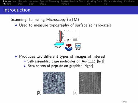
Introduction
Scanning Tunneling Microscopy (STM)
Used to measure topography of surface at nano-scale
Produces two different types of images of interestSelf-assembled cage molecules on Au111 [left]Beta-sheets of peptide on graphite [right]
[2] [3]
3/31
Introduction Methods K-means Spectral Clustering Markov Random Fields Modeling Data Mixture Modeling Conclusion
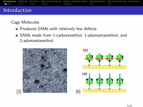
Introduction
Cage Molecules
Produces SAMs with relatively few defects
SAMs made from 1-carboranethiol, 1-adamantanethiol, and2-adamantanethiol
[2] [6]
4/31
Introduction Methods K-means Spectral Clustering Markov Random Fields Modeling Data Mixture Modeling Conclusion
Introduction
Image Segmentation
I0 be the observed image stored as set of pixels and P is auniformity (homogeneity) predicate
Partitioning of I0 into a set of subregions (S1,S2, ...,Sn) wheren⋃
i=1
Si = F with Si ∩ Sj = Ø, i 6= j (1)
P(Si ) = true ∀i and P(Si ∪ Sj) = false, when Si is adjacentto Sj
5/31
Introduction Methods K-means Spectral Clustering Markov Random Fields Modeling Data Mixture Modeling Conclusion
Introduction
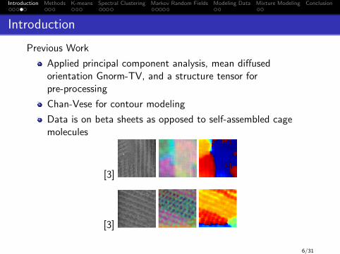
Previous Work
Applied principal component analysis, mean diffusedorientation Gnorm-TV, and a structure tensor forpre-processing
Chan-Vese for contour modeling
Data is on beta sheets as opposed to self-assembled cagemolecules
[3]
[3]
6/31
Introduction Methods K-means Spectral Clustering Markov Random Fields Modeling Data Mixture Modeling Conclusion
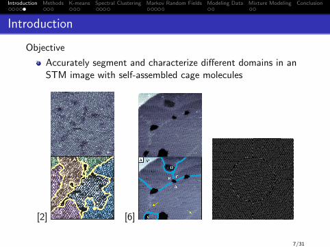
Introduction
Objective
Accurately segment and characterize different domains in anSTM image with self-assembled cage molecules
[2] [6]
7/31

Introduction Methods K-means Spectral Clustering Markov Random Fields Modeling Data Mixture Modeling Conclusion
Methods
Preprocessing
Mexican hat filter separates structure from texture
Hole finder to isolate artifacts
8/31
Introduction Methods K-means Spectral Clustering Markov Random Fields Modeling Data Mixture Modeling Conclusion
Methods
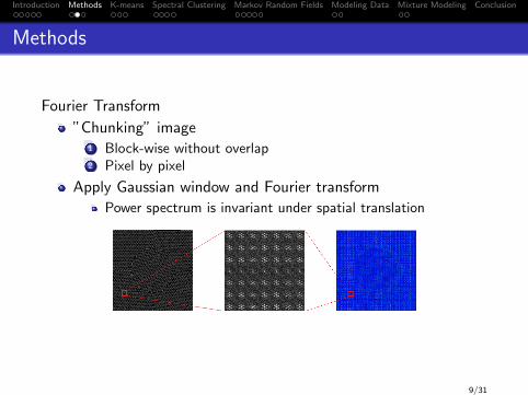
Fourier Transform
”Chunking” image1 Block-wise without overlap2 Pixel by pixel
Apply Gaussian window and Fourier transform
Power spectrum is invariant under spatial translation
9/31
Introduction Methods K-means Spectral Clustering Markov Random Fields Modeling Data Mixture Modeling Conclusion
Methods
Fourier Domain
K-means
Spectral clustering
Bayesian Probability in Fourier Domain
Markov random fields1 Spectral clustering initialization2 Partial labeling
Mixture modeling
Assessing Correctness
Pixel by pixel difference with ground truth
10/31
Introduction Methods K-means Spectral Clustering Markov Random Fields Modeling Data Mixture Modeling Conclusion
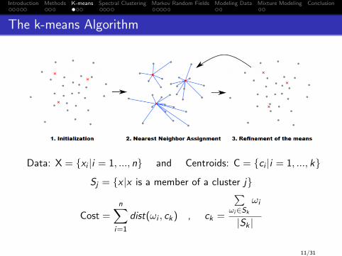
The k-means Algorithm
Data: X = xi |i = 1, ..., n and Centroids: C = ci |i = 1, ..., k
Sj = x |x is a member of a cluster j
Cost =n∑
i=1
dist(ωi , ck) , ck =
∑ωi∈Sk
ωi
|Sk |
11/31
Introduction Methods K-means Spectral Clustering Markov Random Fields Modeling Data Mixture Modeling Conclusion
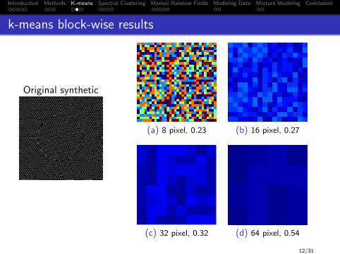
k-means block-wise results
Original synthetic
(a) 8 pixel, 0.23 (b) 16 pixel, 0.27
(c) 32 pixel, 0.32 (d) 64 pixel, 0.54
12/31

Introduction Methods K-means Spectral Clustering Markov Random Fields Modeling Data Mixture Modeling Conclusion
k-means pixel by pixel results
Original Synthetic 32 pixel size, 0.59
13/31
Introduction Methods K-means Spectral Clustering Markov Random Fields Modeling Data Mixture Modeling Conclusion
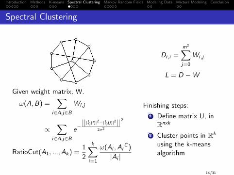
Spectral Clustering
Given weight matrix, W.
ω(A,B) =∑
i∈A,j∈BWi ,j
∝∑
i∈A,j∈Be−|||I0(i)|2−|I0(j)|2||
2σ2
2
RatioCut(A1, ...,Ak) =1
2
k∑i=1
ω(Ai ,AiC )
|Ai |
Di ,i =m2∑j=0
Wi ,j
L = D −W
Finishing steps:
1 Define matrix U, inRnxk
2 Cluster points in Rk
using the k-meansalgorithm
14/31

Introduction Methods K-means Spectral Clustering Markov Random Fields Modeling Data Mixture Modeling Conclusion
Spectral clustering block-wise results
Original synthetic
Various σ at 32 pixel size
(a) σ = log(1.5), 0.69 (b) σ = log(2), 0.54
(c) σ = log(2.5), 0.78 (d) σ = log(3), 0.7215/31
Introduction Methods K-means Spectral Clustering Markov Random Fields Modeling Data Mixture Modeling Conclusion
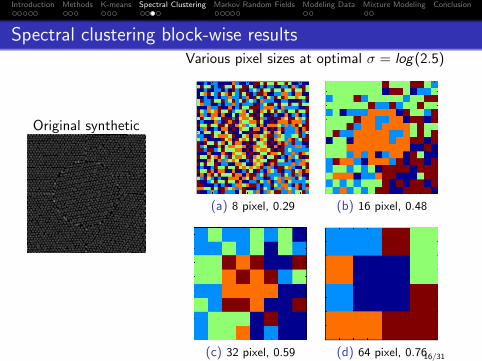
Spectral clustering block-wise results
Original synthetic
Various pixel sizes at optimal σ = log(2.5)
(a) 8 pixel, 0.29 (b) 16 pixel, 0.48
(c) 32 pixel, 0.59 (d) 64 pixel, 0.7616/31

Introduction Methods K-means Spectral Clustering Markov Random Fields Modeling Data Mixture Modeling Conclusion
Spectral clustering pixel by pixel results
(a) Original synthetic (b) σ = 0.071, 32pixel, 0.95
(c) 32 pixel
17/31
Introduction Methods K-means Spectral Clustering Markov Random Fields Modeling Data Mixture Modeling Conclusion
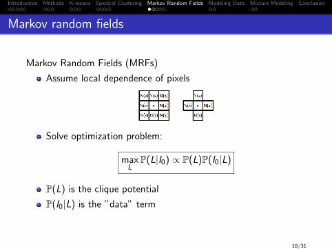
Markov random fields
Markov Random Fields (MRFs)
Assume local dependence of pixels
Solve optimization problem:
maxL
P(L|I0) ∝ P(L)P(I0|L)
P(L) is the clique potential
P(I0|L) is the ”data” term
18/31

Introduction Methods K-means Spectral Clustering Markov Random Fields Modeling Data Mixture Modeling Conclusion
Markov random fields
The Tentative Procedure
Initialize mean (µk) and variance (Σk) for spectrum of eachcluster using k-means
Apply Expectation-Maximization (EM) algorithm on
P(L) =∏x∈I0
P(L(x)|LΩ\x
)=∏x∈I0
P(L(x)|LN(x)
)(2)
∝∏x∈I0
e−λH where H =∑
y∈N(x)
1− 1[L(x)=L(y)] (3)
P(I0|L) =∏x∈I0
N (PS |µk ,Σk) where PS = |I0(x)|2 (4)
Maximize label configuration L in double product forP(L)P(I0|L) across k clusters
Update expected new mean and variance parameters ofspectral clusters
19/31
Introduction Methods K-means Spectral Clustering Markov Random Fields Modeling Data Mixture Modeling Conclusion
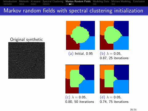
Markov random fields with spectral clustering initialization
Original synthetic
(a) Initial, 0.95 (b) λ = 0.05,0.87, 25 iterations
(c) λ = 0.05,0.80, 50 iterations
(d) λ = 0.05,0.74, 75 iterations
20/31
Introduction Methods K-means Spectral Clustering Markov Random Fields Modeling Data Mixture Modeling Conclusion
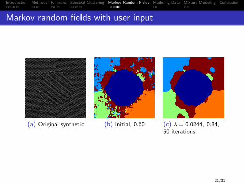
Markov random fields with user input
(a) Original synthetic (b) Initial, 0.60 (c) λ = 0.0244, 0.84,50 iterations
21/31
Introduction Methods K-means Spectral Clustering Markov Random Fields Modeling Data Mixture Modeling Conclusion
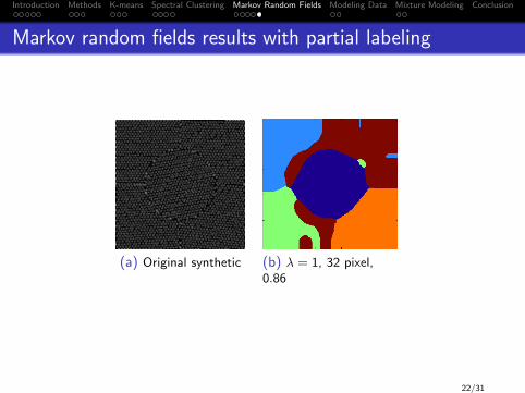
Markov random fields results with partial labeling
(a) Original synthetic (b) λ = 1, 32 pixel,0.86
22/31
Introduction Methods K-means Spectral Clustering Markov Random Fields Modeling Data Mixture Modeling Conclusion
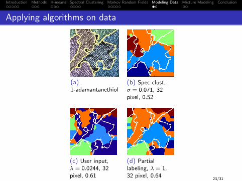
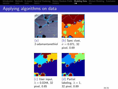
Applying algorithms on data
(a)1-adamantanethiol
(b) Spec clust,σ = 0.071, 32pixel, 0.52
(c) User input,λ = 0.0244, 32pixel, 0.61
(d) Partiallabeling, λ = 1,32 pixel, 0.64
23/31
Introduction Methods K-means Spectral Clustering Markov Random Fields Modeling Data Mixture Modeling Conclusion
Applying algorithms on data
(a)2-adamantanethiol
(b) Spec clust,σ = 0.071, 32pixel, 0.69
(c) User input,λ = 0.0244, 32pixel, 0.85
(d) Partiallabeling, λ = 1,32 pixel, 0.89
24/31
Introduction Methods K-means Spectral Clustering Markov Random Fields Modeling Data Mixture Modeling Conclusion
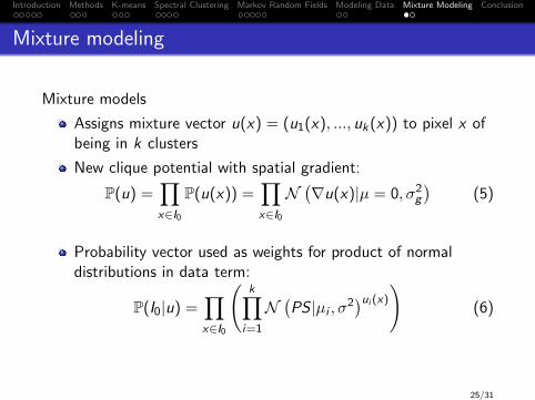
Mixture modeling
Mixture models
Assigns mixture vector u(x) = (u1(x), ..., uk(x)) to pixel x ofbeing in k clusters
New clique potential with spatial gradient:
P(u) =∏x∈I0
P(u(x)) =∏x∈I0
N(∇u(x)|µ = 0, σ2
g
)(5)
Probability vector used as weights for product of normaldistributions in data term:
P(I0|u) =∏x∈I0
(k∏
i=1
N(PS |µi , σ2
)ui (x)
)(6)
25/31
Introduction Methods K-means Spectral Clustering Markov Random Fields Modeling Data Mixture Modeling Conclusion
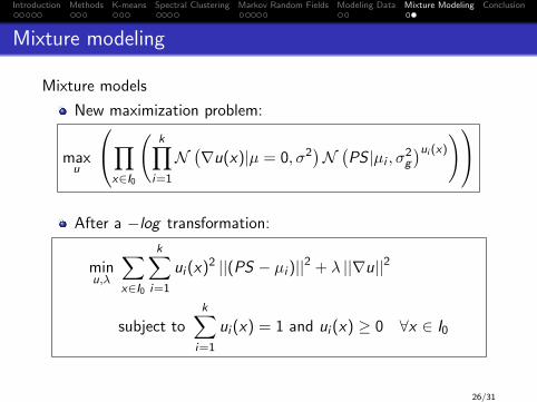
Mixture modeling
Mixture models
New maximization problem:
maxu
∏x∈I0
(k∏
i=1
N(∇u(x)|µ = 0, σ2
)N(PS |µi , σ2
g
)ui (x)
)After a −log transformation:
minu,λ
∑x∈I0
k∑i=1
ui (x)2 ||(PS − µi )||2 + λ ||∇u||2
subject tok∑
i=1
ui (x) = 1 and ui (x) ≥ 0 ∀x ∈ I0
26/31
Introduction Methods K-means Spectral Clustering Markov Random Fields Modeling Data Mixture Modeling Conclusion
Conclusions & Outlook
1 Block by block is not as good as pixel by pixel
2 Spectral clustering works best on synthetic images
3 Markov random fields with k-means manual initialization andpartial labeling works best on microscopy data
4 Optimize Markov random fields to be interactive
5 Attempt mixture modeling
27/31

Introduction Methods K-means Spectral Clustering Markov Random Fields Modeling Data Mixture Modeling Conclusion
References I
Julian Besag.On the statistical analysis of dirty pictures.Journal of the Royal Statistical Society. Series B(Methodological), pages 259–302, 1986.
Arrelaine A. Dameron, Lyndon F. Charles, and Paul S. Weiss.Structures and displacement of 1-adamantanethiolself-assembled monolayers on au 111.Journal of the American Chemical Society,127(24):8697–8704, 2005.
28/31

Introduction Methods K-means Spectral Clustering Markov Random Fields Modeling Data Mixture Modeling Conclusion
References II
Huynh Nen Lim Tawny Meyer Travis Dragomiretskiy, JonathanSiegel Konstantin and Joseph Woodworth.Image analysis and classification in scanning tunnelingmicroscopy.2012.
Rafael C. Gonzalez and R.E. Woods.Digital image processing, 2008.
John A. Hartigan and Manchek A. Wong.Algorithm as 136: A k-means clustering algorithm.Journal of the Royal Statistical Society. Series C (AppliedStatistics), 28(1):100–108, 1979.
29/31

Introduction Methods K-means Spectral Clustering Markov Random Fields Modeling Data Mixture Modeling Conclusion
References III
J. Nathan Hohman, Shelley A. Claridge, Moonhee Kim, andPaul S. Weiss.Cage molecules for self-assembly.Materials Science and Engineering: R: Reports,70(3):188–208, 2010.
Anil K Jain, M. Narasimha Murty, and Patrick J Flynn.Data clustering: a review.ACM computing surveys (CSUR), 31(3):264–323, 1999.
Todd K. Moon.The expectation-maximization algorithm.Signal processing magazine, IEEE, 13(6):47–60, 1996.
30/31
Introduction Methods K-means Spectral Clustering Markov Random Fields Modeling Data Mixture Modeling Conclusion
References IV
Ulrike Von Luxburg.A tutorial on spectral clustering.Statistics and computing, 17(4):395–416, 2007.
31/31