Microsoft Office 2010 Worksheets Excel - Intermediate.docx Page 2 Grouping Worksheets Activate Group Mode Whenever you select more than one worksheet, Excel considers those sheets

Microsoft Office 2010

Excel 2010 Intermediate

Manual

www.catraining.co.uk

- i -

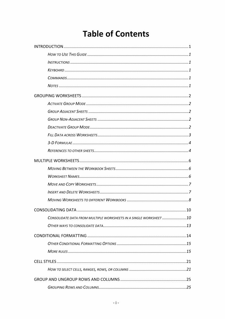
Table of Contents INTRODUCTION .............................................................................................................. 1

HOW TO USE THIS GUIDE ......................................................................................... 1

INSTRUCTIONS ........................................................................................................ 1

KEYBOARD ............................................................................................................. 1

COMMANDS ........................................................................................................... 1

NOTES .................................................................................................................. 1

GROUPING WORKSHEETS .............................................................................................. 2

ACTIVATE GROUP MODE .......................................................................................... 2

GROUP ADJACENT SHEETS ........................................................................................ 2

GROUP NON-ADJACENT SHEETS ................................................................................ 2

DEACTIVATE GROUP MODE ....................................................................................... 2

FILL DATA ACROSS WORKSHEETS ................................................................................ 3

3-D FORMULAE ...................................................................................................... 4

REFERENCES TO OTHER SHEETS ................................................................................... 4

MULTIPLE WORKSHEETS ................................................................................................ 6

MOVING BETWEEN THE WORKBOOK SHEETS ................................................................ 6

WORKSHEET NAMES ................................................................................................ 6

MOVE AND COPY WORKSHEETS ................................................................................. 7

INSERT AND DELETE WORKSHEETS .............................................................................. 7

MOVING WORKSHEETS TO DIFFERENT WORKBOOKS ...................................................... 8

CONSOLIDATING DATA ................................................................................................ 10

CONSOLIDATE DATA FROM MULTIPLE WORKSHEETS IN A SINGLE WORKSHEET ..................... 10

OTHER WAYS TO CONSOLIDATE DATA ......................................................................... 13

CONDITIONAL FORMATTING ....................................................................................... 14

OTHER CONDITIONAL FORMATTING OPTIONS ............................................................. 15

MORE RULES ........................................................................................................ 15

CELL STYLES .................................................................................................................. 21

HOW TO SELECT CELLS, RANGES, ROWS, OR COLUMNS .................................................. 21

GROUP AND UNGROUP ROWS AND COLUMNS .......................................................... 25

GROUPING ROWS AND COLUMNS ............................................................................. 25

- ii -

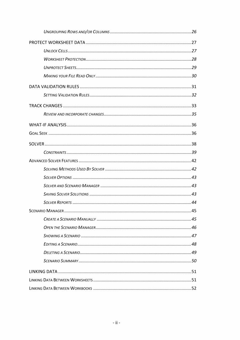
UNGROUPING ROWS AND/OR COLUMNS ................................................................... 26

PROTECT WORKSHEET DATA ....................................................................................... 27

UNLOCK CELLS ...................................................................................................... 27

WORKSHEET PROTECTION ....................................................................................... 28

UNPROTECT SHEETS ............................................................................................... 29

MAKING YOUR FILE READ ONLY ............................................................................... 30

DATA VALIDATION RULES ............................................................................................ 31

SETTING VALIDATION RULES .................................................................................... 32

TRACK CHANGES .......................................................................................................... 33

REVIEW AND INCORPORATE CHANGES ........................................................................ 35

WHAT-IF ANALYSIS ....................................................................................................... 36

GOAL SEEK ...................................................................................................................... 36

SOLVER ......................................................................................................................... 38

CONSTRAINTS ....................................................................................................... 39

ADVANCED SOLVER FEATURES ............................................................................................. 42

SOLVING METHODS USED BY SOLVER ....................................................................... 42

SOLVER OPTIONS .................................................................................................. 43

SOLVER AND SCENARIO MANAGER ........................................................................... 43

SAVING SOLVER SOLUTIONS .................................................................................... 43

SOLVER REPORTS .................................................................................................. 44

SCENARIO MANAGER ......................................................................................................... 45

CREATE A SCENARIO MANUALLY .............................................................................. 45

OPEN THE SCENARIO MANAGER ............................................................................... 46

SHOWING A SCENARIO ........................................................................................... 47

EDITING A SCENARIO .............................................................................................. 48

DELETING A SCENARIO............................................................................................ 49

SCENARIO SUMMARY ............................................................................................. 50

LINKING DATA .............................................................................................................. 51

LINKING DATA BETWEEN WORKSHEETS ................................................................................. 51

LINKING DATA BETWEEN WORKBOOKS ................................................................................. 52

- iii -

Excel - Intermediate.docx Introduction

Page 1

Introduction Excel 2010 is a powerful spreadsheet application that allows users to produce tables containing calculations and graphs. These can range from simple formulae through to complex functions and mathematical models.

How to Use This Guide

This manual should be used as a point of reference following attendance of the Excel 2010 Intermediate level training course. It covers all the topics taught and aims to act as a support aid for any tasks carried out by the user after the course.

The manual is divided into sections, each section covering an aspect of the intermediate course. The table of contents lists the page numbers of each section.

Instructions

Those who have already used a spreadsheet before may not need to read explanations on what each command does, but would rather skip straight to the instructions to find out how to do it. Look out for the arrow icon which precedes a list of instructions.

Keyboard

Keys are referred to throughout the manual in the following way:

[ENTER] – Denotes the return or enter key, [DELETE] – denotes the Delete key and so on.

Where a command requires two keys to be pressed, the manual displays this as follows:

[CTRL] + [P] – this means press the letter “p” while holding down the Control key.

Commands

When a command is referred to in the manual, the following distinctions have been made:

When Ribbon commands are referred to, the manual will refer you to the Ribbon – e.g. “Choose HOME from the Ribbons and then B for bold”.

When dialog box options are referred to, the following style has been used for the text – “In the PAGE RANGE section of the PRINT dialog, click the CURRENT PAGE option”

Dialog box buttons are shaded and boxed – “Click OK to close the PRINT dialog and launch

the print.”

Notes

Within each section, any items that need further explanation or extra attention devoted to them are denoted by shading. For example:

“Excel will not let you close a file that you have not already saved changes to without prompting you to save.”

Grouping Worksheets Excel - Intermediate.docx

Page 2

Grouping Worksheets

Activate Group Mode

Whenever you select more than one worksheet, Excel considers those sheets to be grouped and switches group mode on accordingly. When group mode is active, the grouped worksheet tabs turn white and the word “[group]” appears on the title bar. Any data that you enter and any formatting that you apply will appear on all worksheets in the group in the same positions on each – this is particularly useful if you need to create a “Summary” sheet that will reference the other worksheets three dimensionally.

Group Adjacent Sheets

When the worksheets that you want to group are next to each other, you can use the [SHIFT] key to block select them.

To group adjacent worksheets:

Click the on the first worksheet’s tab that you want to include in your group.

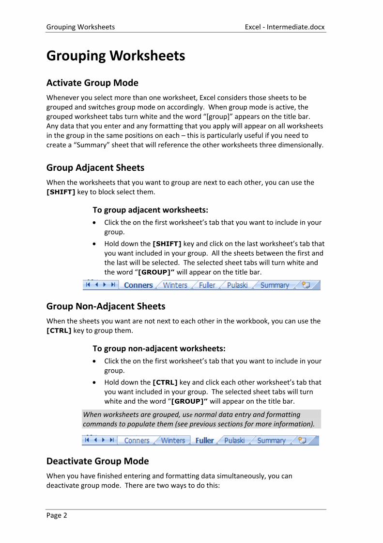
Hold down the [SHIFT] key and click on the last worksheet’s tab that you want included in your group. All the sheets between the first and the last will be selected. The selected sheet tabs will turn white and the word “[GROUP]” will appear on the title bar.

Group Non-Adjacent Sheets

When the sheets you want are not next to each other in the workbook, you can use the [CTRL] key to group them.

To group non-adjacent worksheets:

Click the on the first worksheet’s tab that you want to include in your group.

Hold down the [CTRL] key and click each other worksheet’s tab that you want included in your group. The selected sheet tabs will turn white and the word “[GROUP]” will appear on the title bar.

When worksheets are grouped, use normal data entry and formatting commands to populate them (see previous sections for more information).

Deactivate Group Mode

When you have finished entering and formatting data simultaneously, you can deactivate group mode. There are two ways to do this:

Excel - Intermediate.docx Grouping Worksheets

Page 3

To deactivate group mode:

Click on a sheet tab that is not currently grouped (non white).

Or Click the right mouse button over any sheet tab and choose Ungroup

Sheets from the shortcut menu.

Fill Data across Worksheets

You can copy data to the same position on multiple sheets using the Fill command. This is particularly useful if you need to decide what gets copied (everything, or just the formats). It also saves time for those occasions where you accidentally deactivated group mode, typed your entries and then realised that they are only on one page!

To fill across worksheets:

Select the cells you want to copy to the other worksheet(s)

Select the worksheets you want the copy to appear on by clicking the

sheet tabs (use [SHIFT] to block select or [CTRL] to pick non-adjacent

pages)

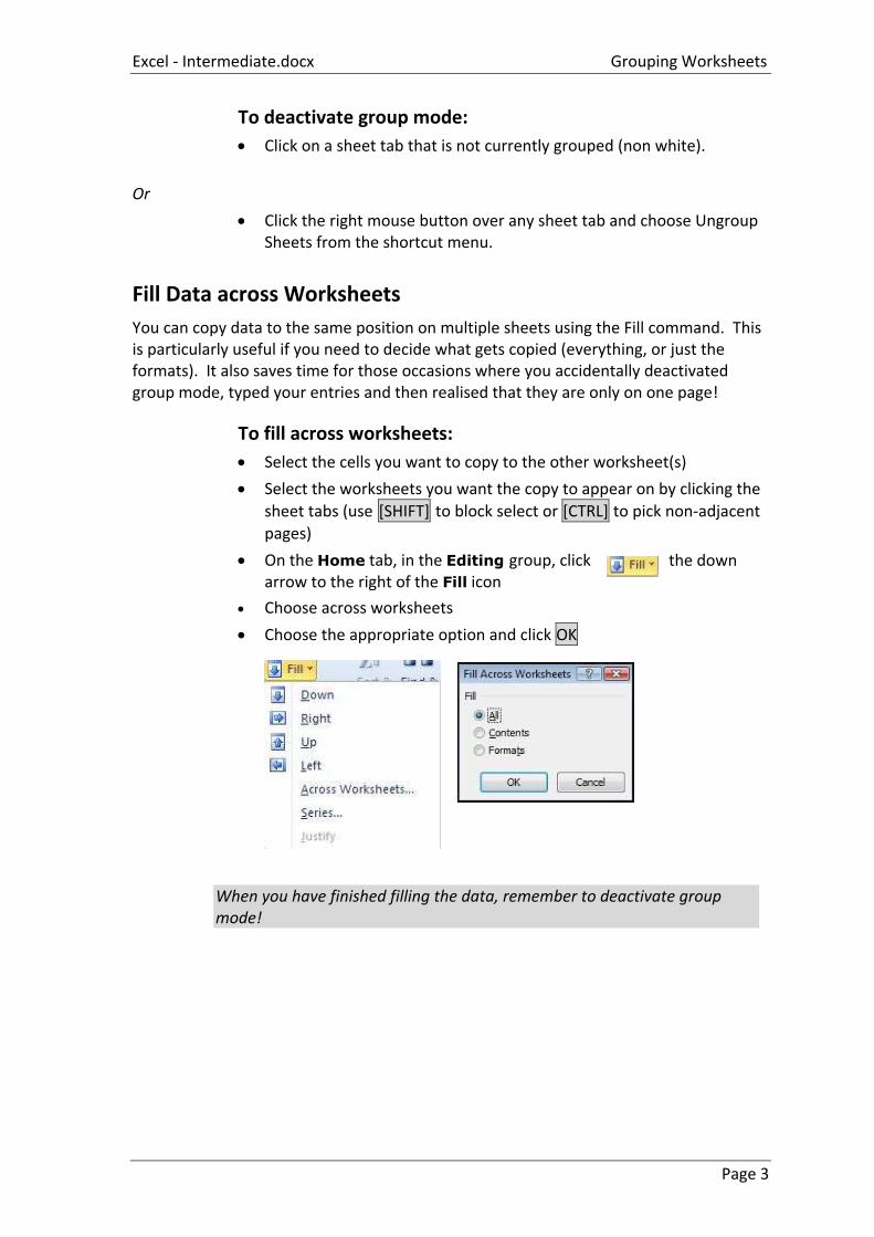
On the Home tab, in the Editing group, click the down arrow to the right of the Fill icon

Choose across worksheets

Choose the appropriate option and click OK

When you have finished filling the data, remember to deactivate group mode!

Grouping Worksheets Excel - Intermediate.docx

Page 4

3-D Formulae

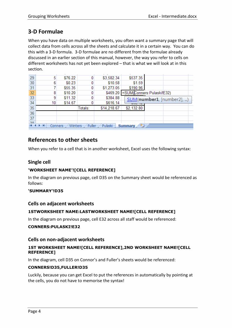
When you have data on multiple worksheets, you often want a summary page that will collect data from cells across all the sheets and calculate it in a certain way. You can do this with a 3-D formula. 3-D formulae are no different from the formulae already discussed in an earlier section of this manual, however, the way you refer to cells on different worksheets has not yet been explored – that is what we will look at in this section.

References to other sheets

When you refer to a cell that is in another worksheet, Excel uses the following syntax:

Single cell

‘WORKSHEET NAME’![CELL REFERENCE]

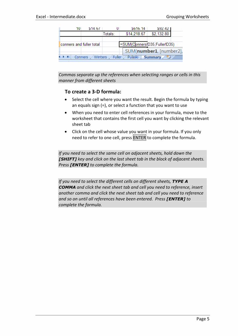
In the diagram on previous page, cell D35 on the Summary sheet would be referenced as follows:

‘SUMMARY’!D35

Cells on adjacent worksheets

1STWORKSHEET NAME:LASTWORKSHEET NAME![CELL REFERENCE]

In the diagram on previous page, cell E32 across all staff would be referenced:

CONNERS:PULASKI!E32

Cells on non-adjacent worksheets

1ST WORKSHEET NAME![CELL REFERENCE],2ND WORKSHEET NAME![CELL

REFERENCE]

In the diagram, cell D35 on Connor’s and Fuller’s sheets would be referenced:

CONNERS!D35,FULLER!D35

Luckily, because you can get Excel to put the references in automatically by pointing at the cells, you do not have to memorise the syntax!

Excel - Intermediate.docx Grouping Worksheets

Page 5

Commas separate up the references when selecting ranges or cells in this manner from different sheets

To create a 3-D formula:

Select the cell where you want the result. Begin the formula by typing an equals sign (=), or select a function that you want to use

When you need to enter cell references in your formula, move to the worksheet that contains the first cell you want by clicking the relevant sheet tab

Click on the cell whose value you want in your formula. If you only

need to refer to one cell, press ENTER to complete the formula.

If you need to select the same cell on adjacent sheets, hold down the [SHIFT] key and click on the last sheet tab in the block of adjacent sheets. Press [ENTER] to complete the formula.

If you need to select the different cells on different sheets, TYPE A

COMMA and click the next sheet tab and cell you need to reference, insert another comma and click the next sheet tab and cell you need to reference and so on until all references have been entered. Press [ENTER] to complete the formula.

Multiple Worksheets Excel - Intermediate.docx

Page 6

Multiple Worksheets When you create a new workbook, Excel gives you multiple pages within that workbook called worksheets. The number of worksheets you get defaults to 3, but you can change that (see the section on customisation for more information). The worksheets are useful when you want to store information under common column headings but need to split it up, (for example by month, week or by department).

When the same data needs to be entered on several worksheets, you can use Group mode which forces data that you type on one worksheet appear on all selected sheets. When Group mode is active, any formatting that you apply to the active worksheet also gets applied to the selected sheets.

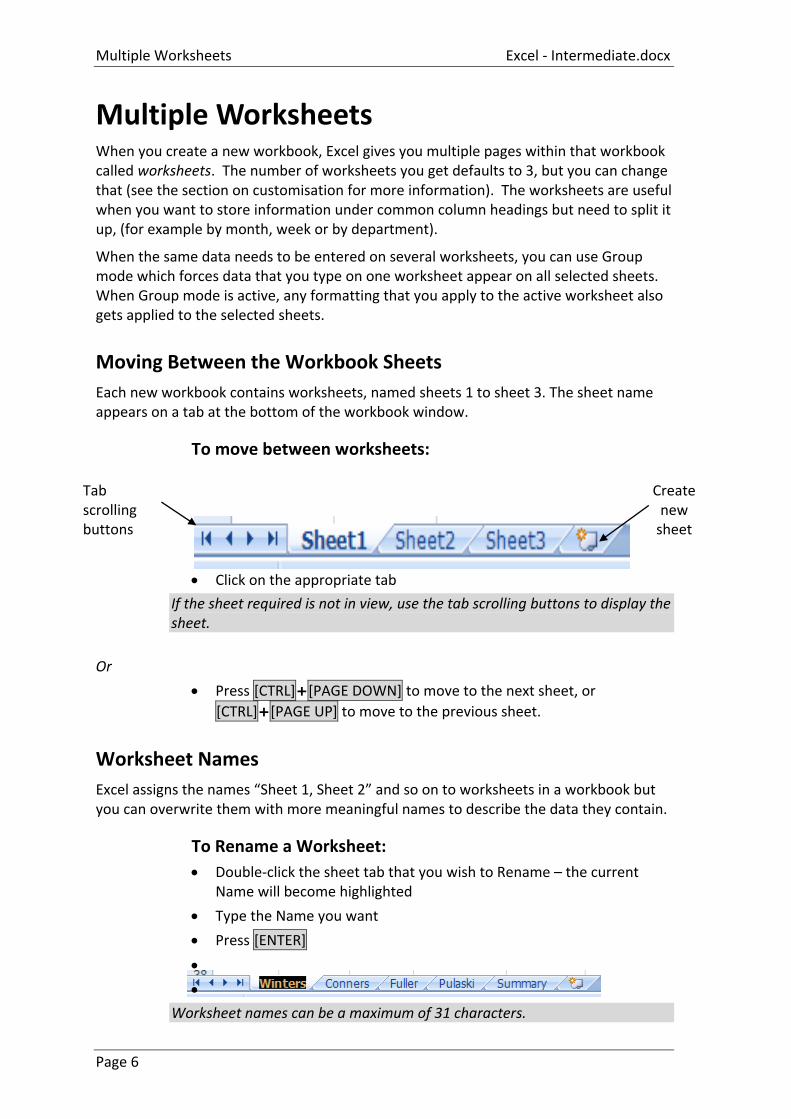
Moving Between the Workbook Sheets

Each new workbook contains worksheets, named sheets 1 to sheet 3. The sheet name appears on a tab at the bottom of the workbook window.

To move between worksheets:

Click on the appropriate tab

If the sheet required is not in view, use the tab scrolling buttons to display the sheet.

Or Press [CTRL]+[PAGE DOWN] to move to the next sheet, or

[CTRL]+[PAGE UP] to move to the previous sheet.

Worksheet Names

Excel assigns the names “Sheet 1, Sheet 2” and so on to worksheets in a workbook but you can overwrite them with more meaningful names to describe the data they contain.

To Rename a Worksheet:

Double-click the sheet tab that you wish to Rename – the current Name will become highlighted

Type the Name you want

Press [ENTER]

Worksheet names can be a maximum of 31 characters.

Tab scrolling buttons

Create new

sheet

Excel - Intermediate.docx Multiple Worksheets

Page 7

Move and Copy Worksheets

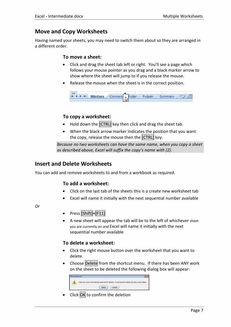
Having named your sheets, you may need to switch them about so they are arranged in a different order.

To move a sheet:

Click and drag the sheet tab left or right. You’ll see a page which follows your mouse pointer as you drag and a black marker arrow to show where the sheet will jump to if you release the mouse.

Release the mouse when the sheet is in the correct position.

To copy a worksheet:

Hold down the [CTRL] key then click and drag the sheet tab.

When the black arrow marker indicates the position that you want

the copy, release the mouse then the [CTRL] key.

Because no two worksheets can have the same name, when you copy a sheet as described above, Excel will suffix the copy’s name with (2).

Insert and Delete Worksheets

You can add and remove worksheets to and from a workbook as required.

To add a worksheet:

Click on the last tab of the sheets this is a create new worksheet tab

Excel will name it initially with the next sequential number available

Or

Press [Shift]+[F11]

A new sheet will appear the tab will be to the left of whichever sheet

you are currently on and Excel will name it initially with the next sequential number available

To delete a worksheet:

Click the right mouse button over the worksheet that you want to delete.

Choose Delete from the shortcut menu. If there has been ANY work

on the sheet to be deleted the following dialog box will appear:

Click OK to confirm the deletion

Multiple Worksheets Excel - Intermediate.docx

Page 8

Moving Worksheets to different Workbooks

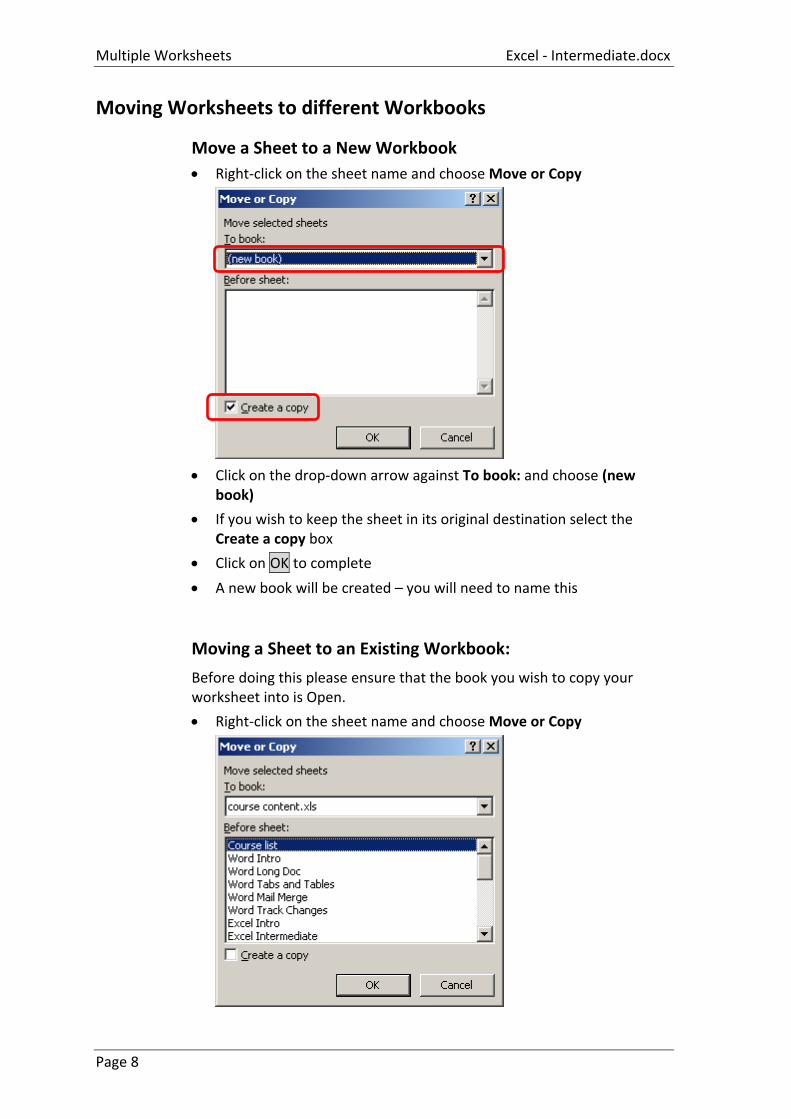
Move a Sheet to a New Workbook

Right-click on the sheet name and choose Move or Copy

Click on the drop-down arrow against To book: and choose (new

book)

If you wish to keep the sheet in its original destination select the Create a copy box

Click on OK to complete

A new book will be created – you will need to name this

Moving a Sheet to an Existing Workbook:

Before doing this please ensure that the book you wish to copy your worksheet into is Open.

Right-click on the sheet name and choose Move or Copy

Excel - Intermediate.docx Multiple Worksheets

Page 9

Click on the drop-down arrow in the To book: section and choose the Workbook you wish to copy the sheet into

If you wish to also keep the sheet in its original destination select the Create a copy box

In the Before sheet: section choose the sheet you wish your worksheet to go before

Click on OK to complete

Consolidating Data Excel - Intermediate.docx

Page 10

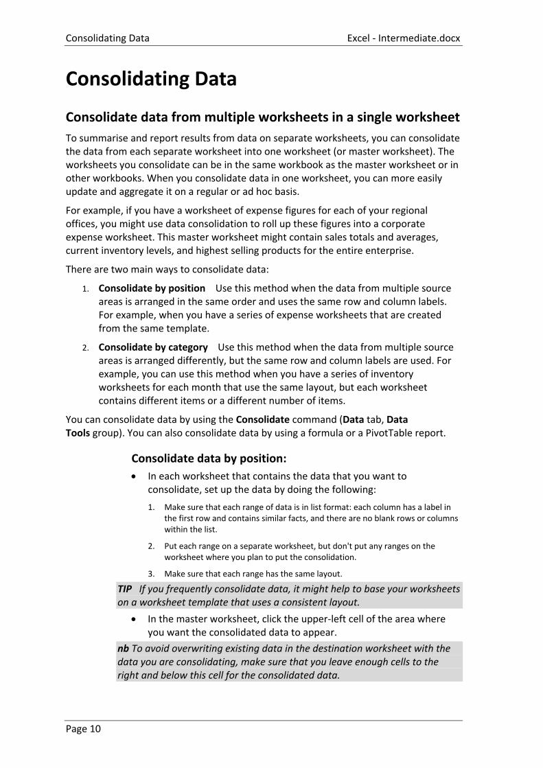
Consolidating Data

Consolidate data from multiple worksheets in a single worksheet

To summarise and report results from data on separate worksheets, you can consolidate the data from each separate worksheet into one worksheet (or master worksheet). The worksheets you consolidate can be in the same workbook as the master worksheet or in other workbooks. When you consolidate data in one worksheet, you can more easily update and aggregate it on a regular or ad hoc basis.

For example, if you have a worksheet of expense figures for each of your regional offices, you might use data consolidation to roll up these figures into a corporate expense worksheet. This master worksheet might contain sales totals and averages, current inventory levels, and highest selling products for the entire enterprise.

There are two main ways to consolidate data:

1. Consolidate by position Use this method when the data from multiple source areas is arranged in the same order and uses the same row and column labels. For example, when you have a series of expense worksheets that are created from the same template.

2. Consolidate by category Use this method when the data from multiple source areas is arranged differently, but the same row and column labels are used. For example, you can use this method when you have a series of inventory worksheets for each month that use the same layout, but each worksheet contains different items or a different number of items.

You can consolidate data by using the Consolidate command (Data tab, Data Tools group). You can also consolidate data by using a formula or a PivotTable report.

Consolidate data by position:

In each worksheet that contains the data that you want to consolidate, set up the data by doing the following:

1. Make sure that each range of data is in list format: each column has a label in the first row and contains similar facts, and there are no blank rows or columns within the list.

2. Put each range on a separate worksheet, but don't put any ranges on the worksheet where you plan to put the consolidation.

3. Make sure that each range has the same layout.

TIP If you frequently consolidate data, it might help to base your worksheets on a worksheet template that uses a consistent layout.

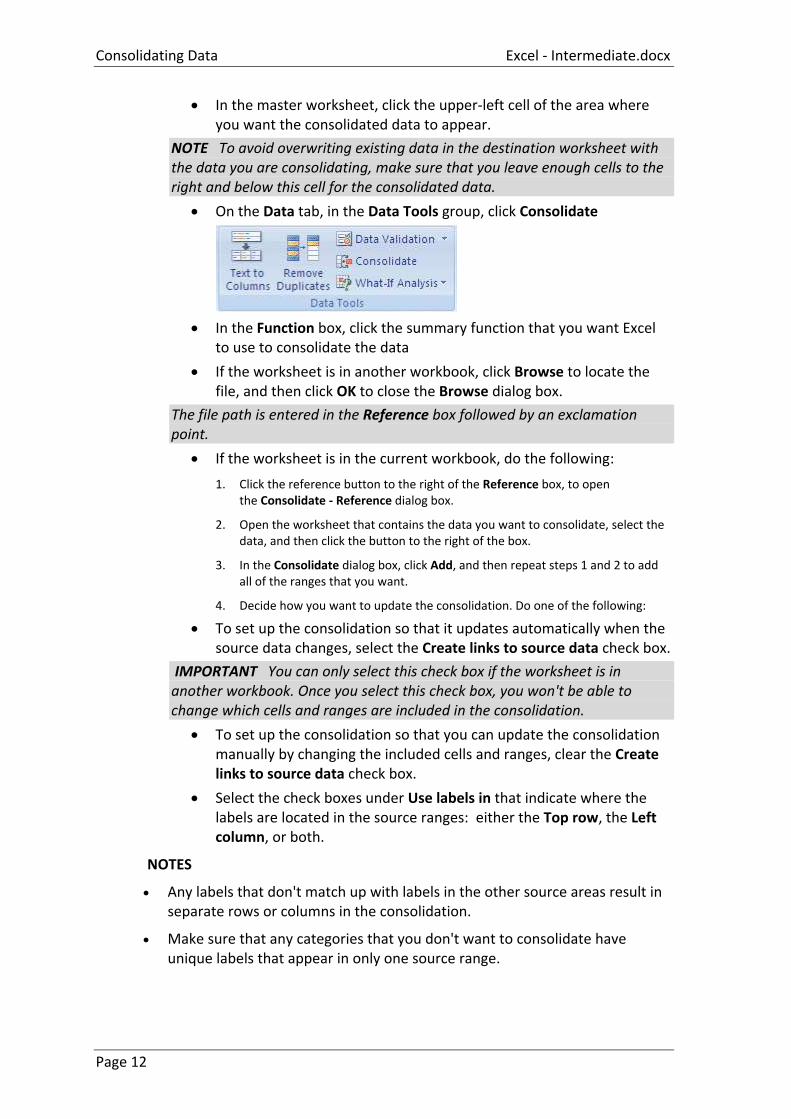
In the master worksheet, click the upper-left cell of the area where you want the consolidated data to appear.

nb To avoid overwriting existing data in the destination worksheet with the data you are consolidating, make sure that you leave enough cells to the right and below this cell for the consolidated data.

Excel - Intermediate.docx Consolidating Data

Page 11

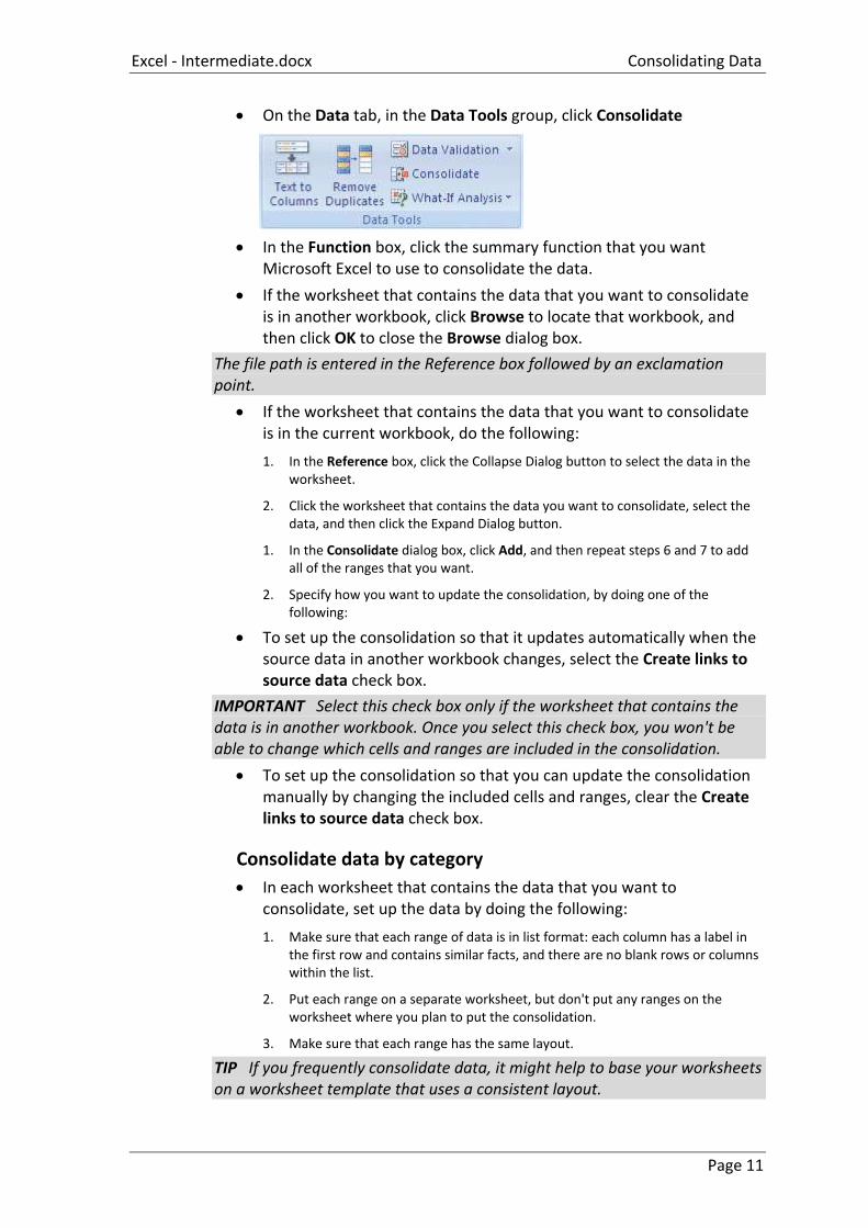
On the Data tab, in the Data Tools group, click Consolidate

In the Function box, click the summary function that you want Microsoft Excel to use to consolidate the data.

If the worksheet that contains the data that you want to consolidate is in another workbook, click Browse to locate that workbook, and then click OK to close the Browse dialog box.

The file path is entered in the Reference box followed by an exclamation point.

If the worksheet that contains the data that you want to consolidate is in the current workbook, do the following:

1. In the Reference box, click the Collapse Dialog button to select the data in the worksheet.

2. Click the worksheet that contains the data you want to consolidate, select the data, and then click the Expand Dialog button.

1. In the Consolidate dialog box, click Add, and then repeat steps 6 and 7 to add all of the ranges that you want.

2. Specify how you want to update the consolidation, by doing one of the following:

To set up the consolidation so that it updates automatically when the source data in another workbook changes, select the Create links to source data check box.

IMPORTANT Select this check box only if the worksheet that contains the data is in another workbook. Once you select this check box, you won't be able to change which cells and ranges are included in the consolidation.

To set up the consolidation so that you can update the consolidation manually by changing the included cells and ranges, clear the Create links to source data check box.

Consolidate data by category

In each worksheet that contains the data that you want to consolidate, set up the data by doing the following:

1. Make sure that each range of data is in list format: each column has a label in the first row and contains similar facts, and there are no blank rows or columns within the list.

2. Put each range on a separate worksheet, but don't put any ranges on the worksheet where you plan to put the consolidation.

3. Make sure that each range has the same layout.

TIP If you frequently consolidate data, it might help to base your worksheets on a worksheet template that uses a consistent layout.

Consolidating Data Excel - Intermediate.docx

Page 12

In the master worksheet, click the upper-left cell of the area where you want the consolidated data to appear.

NOTE To avoid overwriting existing data in the destination worksheet with the data you are consolidating, make sure that you leave enough cells to the right and below this cell for the consolidated data.

On the Data tab, in the Data Tools group, click Consolidate

In the Function box, click the summary function that you want Excel to use to consolidate the data

If the worksheet is in another workbook, click Browse to locate the file, and then click OK to close the Browse dialog box.

The file path is entered in the Reference box followed by an exclamation point.

If the worksheet is in the current workbook, do the following:

1. Click the reference button to the right of the Reference box, to open the Consolidate - Reference dialog box.

2. Open the worksheet that contains the data you want to consolidate, select the data, and then click the button to the right of the box.

3. In the Consolidate dialog box, click Add, and then repeat steps 1 and 2 to add all of the ranges that you want.

4. Decide how you want to update the consolidation. Do one of the following:

To set up the consolidation so that it updates automatically when the source data changes, select the Create links to source data check box.

IMPORTANT You can only select this check box if the worksheet is in another workbook. Once you select this check box, you won't be able to change which cells and ranges are included in the consolidation.

To set up the consolidation so that you can update the consolidation manually by changing the included cells and ranges, clear the Create links to source data check box.

Select the check boxes under Use labels in that indicate where the labels are located in the source ranges: either the Top row, the Left column, or both.

NOTES

Any labels that don't match up with labels in the other source areas result in separate rows or columns in the consolidation.

Make sure that any categories that you don't want to consolidate have unique labels that appear in only one source range.

Excel - Intermediate.docx Consolidating Data

Page 13

Other ways to consolidate data

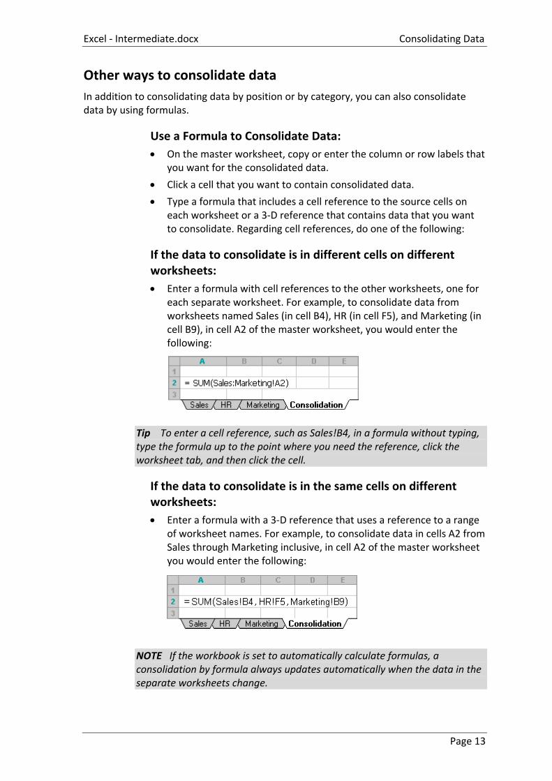
In addition to consolidating data by position or by category, you can also consolidate data by using formulas.

Use a Formula to Consolidate Data:

On the master worksheet, copy or enter the column or row labels that you want for the consolidated data.

Click a cell that you want to contain consolidated data.

Type a formula that includes a cell reference to the source cells on each worksheet or a 3-D reference that contains data that you want to consolidate. Regarding cell references, do one of the following:

If the data to consolidate is in different cells on different worksheets:

Enter a formula with cell references to the other worksheets, one for each separate worksheet. For example, to consolidate data from worksheets named Sales (in cell B4), HR (in cell F5), and Marketing (in cell B9), in cell A2 of the master worksheet, you would enter the following:

Tip To enter a cell reference, such as Sales!B4, in a formula without typing, type the formula up to the point where you need the reference, click the worksheet tab, and then click the cell.

If the data to consolidate is in the same cells on different worksheets:

Enter a formula with a 3-D reference that uses a reference to a range of worksheet names. For example, to consolidate data in cells A2 from Sales through Marketing inclusive, in cell A2 of the master worksheet you would enter the following:

NOTE If the workbook is set to automatically calculate formulas, a consolidation by formula always updates automatically when the data in the separate worksheets change.

Conditional Formatting Excel - Intermediate.docx

Page 14

Conditional Formatting Conditional formatting helps to answer these questions by making it easy to highlight interesting cells or ranges of cells, emphasize unusual values, and visualize data by using data bars, colour scales and icon sets. A conditional format changes the appearance of a cell range based on a condition (or criteria). If the condition is true, the cell range is formatted based on that condition; if the conditional is false, the cell range is not formatted based on that condition.

When creating a conditional format, you can reference other cells in a worksheet, such as =FY2006!A5, but you cannot use external references to another workbook.

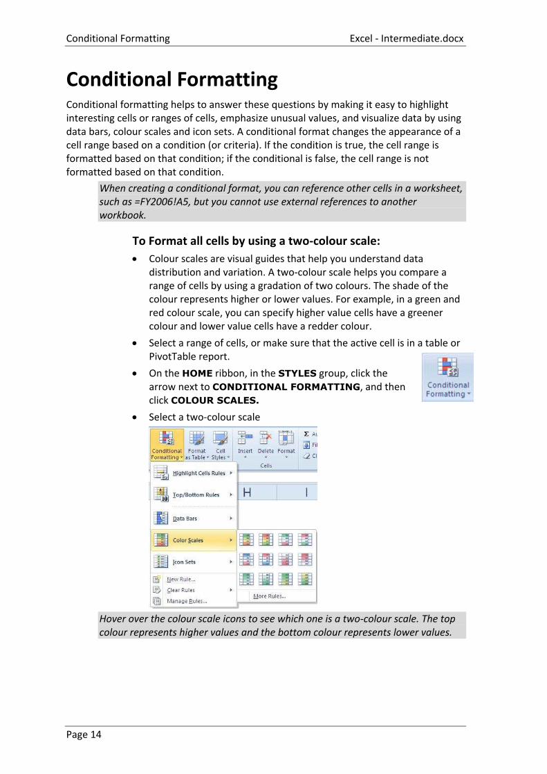
To Format all cells by using a two-colour scale:

Colour scales are visual guides that help you understand data distribution and variation. A two-colour scale helps you compare a range of cells by using a gradation of two colours. The shade of the colour represents higher or lower values. For example, in a green and red colour scale, you can specify higher value cells have a greener colour and lower value cells have a redder colour.

Select a range of cells, or make sure that the active cell is in a table or PivotTable report.

On the HOME ribbon, in the STYLES group, click the arrow next to CONDITIONAL FORMATTING, and then click COLOUR SCALES.

Select a two-colour scale

Hover over the colour scale icons to see which one is a two-colour scale. The top colour represents higher values and the bottom colour represents lower values.

Excel - Intermediate.docx Conditional Formatting

Page 15

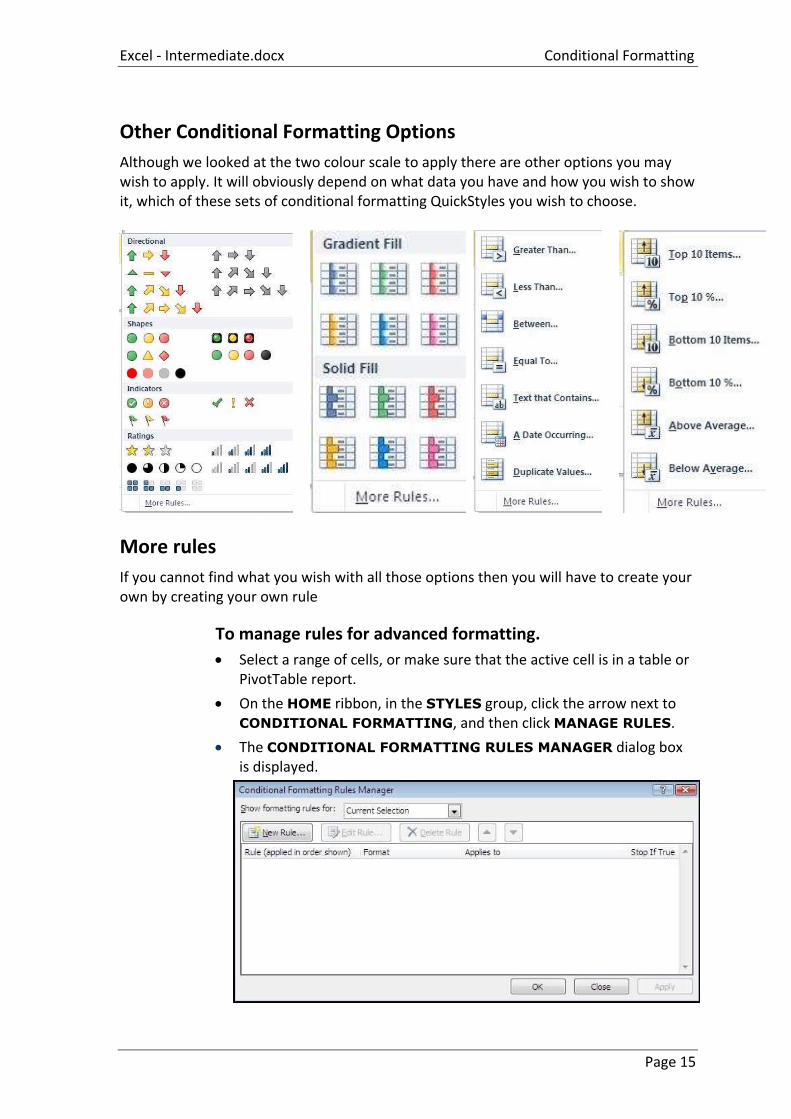
Other Conditional Formatting Options

Although we looked at the two colour scale to apply there are other options you may wish to apply. It will obviously depend on what data you have and how you wish to show it, which of these sets of conditional formatting QuickStyles you wish to choose.

More rules

If you cannot find what you wish with all those options then you will have to create your own by creating your own rule

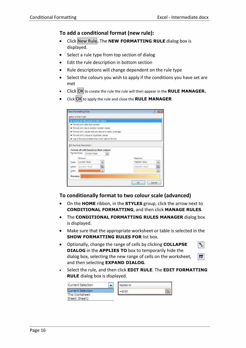
To manage rules for advanced formatting.


On the HOME ribbon, in the STYLES group, click the arrow next to CONDITIONAL FORMATTING, and then click MANAGE RULES.

The CONDITIONAL FORMATTING RULES MANAGER dialog box is displayed.


Page 16

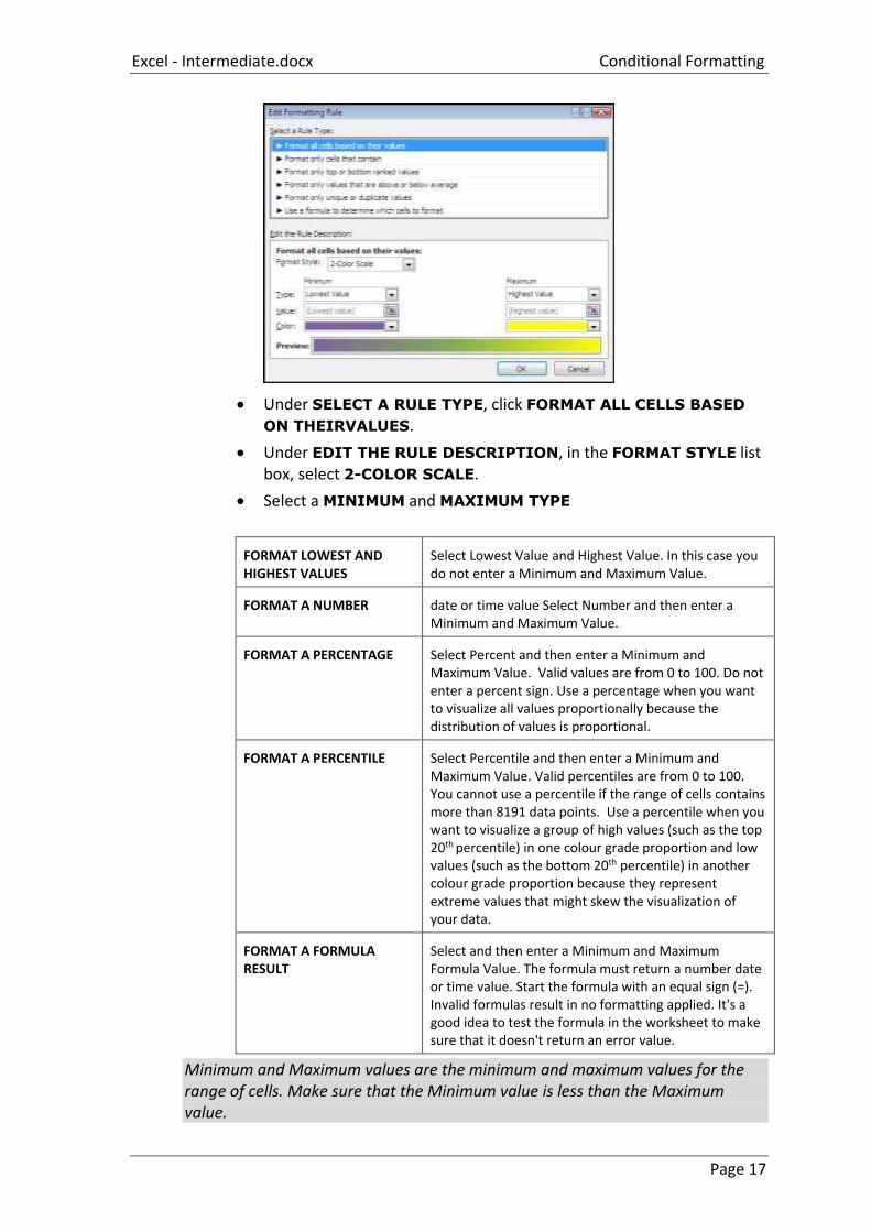
To add a conditional format (new rule):

Click New Rule. The NEW FORMATTING RULE dialog box is

displayed.

Select a rule type from top section of dialog

Edit the rule description in bottom section

Rule descriptions will change dependent on the rule type

Select the colours you wish to apply if the conditions you have set are met

Click OK to create the rule the rule will then appear in the RULE MANAGER.

Click OK to apply the rule and close the RULE MANAGER

To conditionally format to two colour scale (advanced)

On the HOME ribbon, in the STYLES group, click the arrow next to CONDITIONAL FORMATTING, and then click MANAGE RULES.

The CONDITIONAL FORMATTING RULES MANAGER dialog box is displayed.

Make sure that the appropriate worksheet or table is selected in the SHOW FORMATTING RULES FOR list box.

Optionally, change the range of cells by clicking COLLAPSE

DIALOG in the APPLIES TO box to temporarily hide the dialog box, selecting the new range of cells on the worksheet, and then selecting EXPAND DIALOG.

Select the rule, and then click EDIT RULE. The EDIT FORMATTING

RULE dialog box is displayed.


Page 17

Under SELECT A RULE TYPE, click FORMAT ALL CELLS BASED

ON THEIRVALUES.

Under EDIT THE RULE DESCRIPTION, in the FORMAT STYLE list box, select 2-COLOR SCALE.

Select a MINIMUM and MAXIMUM TYPE

FORMAT LOWEST AND HIGHEST VALUES

Select Lowest Value and Highest Value. In this case you do not enter a Minimum and Maximum Value.

FORMAT A NUMBER date or time value Select Number and then enter a Minimum and Maximum Value.

FORMAT A PERCENTAGE Select Percent and then enter a Minimum and Maximum Value. Valid values are from 0 to 100. Do not enter a percent sign. Use a percentage when you want to visualize all values proportionally because the distribution of values is proportional.

FORMAT A PERCENTILE Select Percentile and then enter a Minimum and Maximum Value. Valid percentiles are from 0 to 100. You cannot use a percentile if the range of cells contains more than 8191 data points. Use a percentile when you want to visualize a group of high values (such as the top 20th percentile) in one colour grade proportion and low values (such as the bottom 20th percentile) in another colour grade proportion because they represent extreme values that might skew the visualization of your data.

FORMAT A FORMULA RESULT

Select and then enter a Minimum and Maximum Formula Value. The formula must return a number date or time value. Start the formula with an equal sign (=). Invalid formulas result in no formatting applied. It's a good idea to test the formula in the worksheet to make sure that it doesn't return an error value.

Minimum and Maximum values are the minimum and maximum values for the range of cells. Make sure that the Minimum value is less than the Maximum value.


Page 18

You can choose a different Minimum and Maximum Type. For example, you can choose a Minimum Number and Maximum Percent.

To choose a MINIMUM and MAXIMUM colour scale, click COLOUR for each, and then select a colour. If you want to choose additional colours or create a custom colour, click MORE COLOURS.

The colour scale that you select is displayed in the PREVIEW box.

Click OK to return to the rule manager

Click OK to apply the new rule to selected cells and close rule manager.

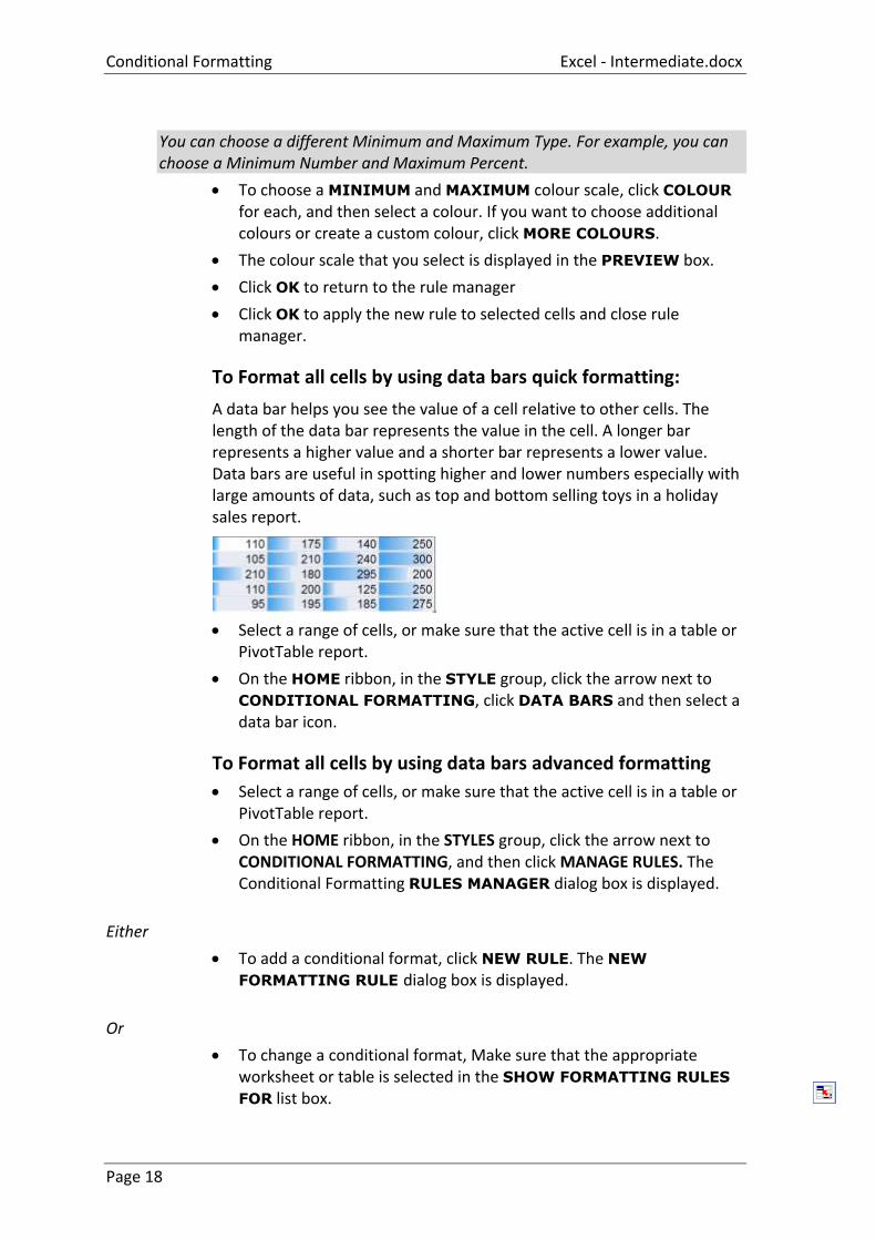
To Format all cells by using data bars quick formatting:

A data bar helps you see the value of a cell relative to other cells. The length of the data bar represents the value in the cell. A longer bar represents a higher value and a shorter bar represents a lower value. Data bars are useful in spotting higher and lower numbers especially with large amounts of data, such as top and bottom selling toys in a holiday sales report.


On the HOME ribbon, in the STYLE group, click the arrow next to CONDITIONAL FORMATTING, click DATA BARS and then select a data bar icon.

To Format all cells by using data bars advanced formatting


On the HOME ribbon, in the STYLES group, click the arrow next to CONDITIONAL FORMATTING, and then click MANAGE RULES. The Conditional Formatting RULES MANAGER dialog box is displayed.

Either

To add a conditional format, click NEW RULE. The NEW

FORMATTING RULE dialog box is displayed.

Or

To change a conditional format, Make sure that the appropriate worksheet or table is selected in the SHOW FORMATTING RULES

FOR list box.


Page 19

Optionally, change the range of cells by clicking COLLAPSE DIALOG in the APPLIES TO box to temporarily hide the dialog box, selecting the new range of cells on the worksheet, and then selecting EXPAND

DIALOG .

Select the rule, and then click EDIT RULE. The EDIT FORMATTING RULE dialog box is displayed.

Under SELECT A RULE TYPE, click FORMAT ALL CELLS BASED

ON THEIR VALUES.

Under EDIT THE RULE DESCRIPTION, in the FORMAT STYLE list box, select DATA BAR.

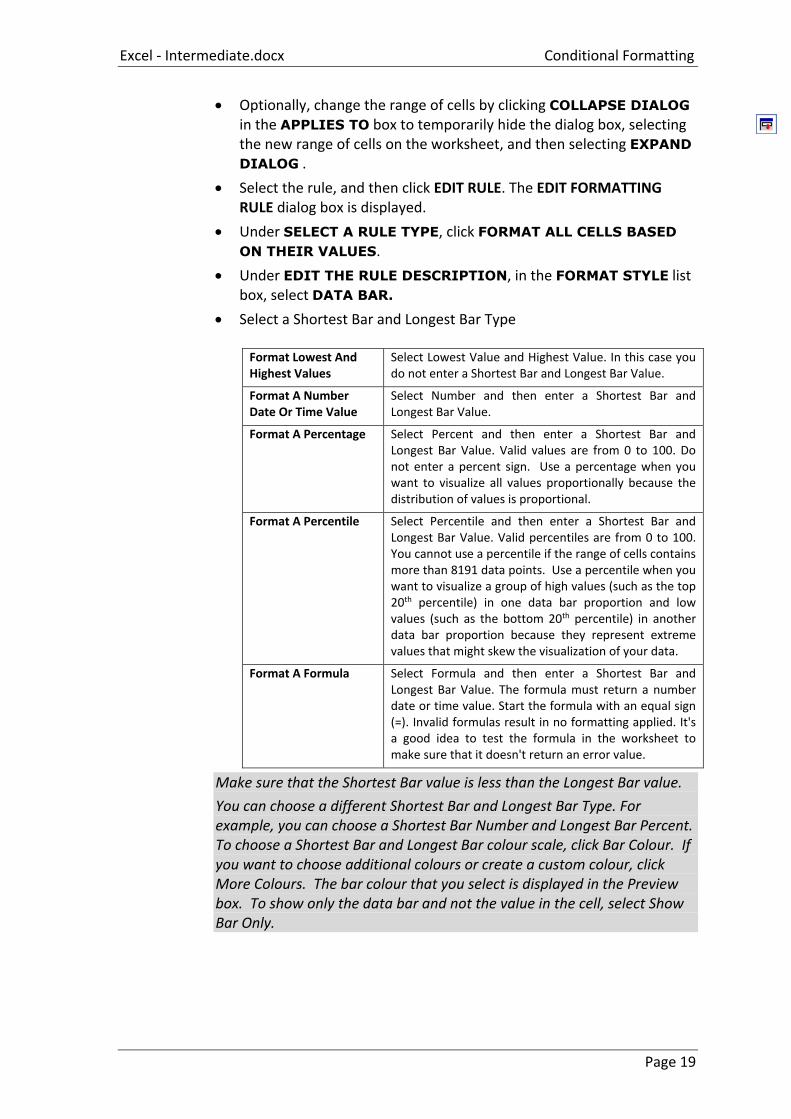
Select a Shortest Bar and Longest Bar Type

Format Lowest And Highest Values

Select Lowest Value and Highest Value. In this case you do not enter a Shortest Bar and Longest Bar Value.

Format A Number Date Or Time Value

Select Number and then enter a Shortest Bar and Longest Bar Value.

Format A Percentage Select Percent and then enter a Shortest Bar and Longest Bar Value. Valid values are from 0 to 100. Do not enter a percent sign. Use a percentage when you want to visualize all values proportionally because the distribution of values is proportional.

Format A Percentile Select Percentile and then enter a Shortest Bar and Longest Bar Value. Valid percentiles are from 0 to 100. You cannot use a percentile if the range of cells contains more than 8191 data points. Use a percentile when you want to visualize a group of high values (such as the top 20th percentile) in one data bar proportion and low values (such as the bottom 20th percentile) in another data bar proportion because they represent extreme values that might skew the visualization of your data.

Format A Formula Select Formula and then enter a Shortest Bar and Longest Bar Value. The formula must return a number date or time value. Start the formula with an equal sign (=). Invalid formulas result in no formatting applied. It's a good idea to test the formula in the worksheet to make sure that it doesn't return an error value.

Make sure that the Shortest Bar value is less than the Longest Bar value.

You can choose a different Shortest Bar and Longest Bar Type. For example, you can choose a Shortest Bar Number and Longest Bar Percent. To choose a Shortest Bar and Longest Bar colour scale, click Bar Colour. If you want to choose additional colours or create a custom colour, click More Colours. The bar colour that you select is displayed in the Preview box. To show only the data bar and not the value in the cell, select Show Bar Only.


Page 20

To clear conditional formats (worksheet):

On the HOME ribbon, in the STYLES group, click the arrow next to CONDITIONAL FORMATTING, and then click CLEAR RULES.

Click ENTIRE SHEET.

To clear conditional formats (A range of cells, table, or PivotTable):

Select the range of cells, table or PivotTable for which you want to clear conditional formats.

On the HOME ribbon, in the STYLES group, click the arrow next to CONDITIONAL FORMATTING, and then click CLEAR RULES.

Depending on what you have selected, click SELECTED CELLS,

THIS TABLE or THIS PIVOTTABLE.

Excel - Intermediate.docx Cell Styles

Page 21

Cell Styles To apply several formats in one step, and to ensure that cells have consistent formatting, you can use a cell style. A cell style is a defined set of formatting characteristics, such as fonts and font sizes, number formats, cell borders and cell shading. To prevent anyone from making changes to specific cells, you can also use a cell style that locks cells. Microsoft Office Excel has several built-in cell styles that you can apply or modify. You can also modify or duplicate a cell style to create your own, custom cell style.

Cell styles are based on the document theme that is applied to the entire workbook. When you switch to another document theme, the cell styles are updated to match the new document theme.

How to select cells, ranges, rows, or columns

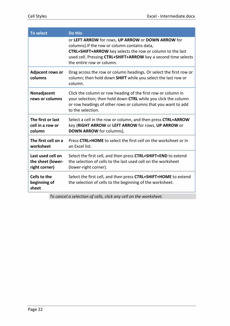
To select Do this

A single cell Click the cell, or press the arrow keys to move to the cell.

A range of cells Click the first cell in the range, and then drag to the last cell, or hold down SHIFT while you press the arrow keys to extend the selection.

You can also select the first cell in the range, and then press F8 to extend the selection by using the arrow keys. To stop extending the selection, press F8 again.

A large range of cells

Click the first cell in the range, and then hold down SHIFT while you click the last cell in the range. You can scroll to make the last cell visible.

All cells on a worksheet

Click the Select All button. To select the entire worksheet, you can also press CTRL+A. If the worksheet contains data, CTRL+A selects the current region. Pressing CTRL+A a second time selects the entire worksheet.

Nonadjacent cells or cell ranges

Select the first cell or range of cells, and then hold down CTRL while you select the other cells or ranges. You can also select the first cell or range of cells, and then press SHIFT+F8 to add another nonadjacent cell or range to the selection. To stop adding cells or ranges to the selection, press SHIFT+F8 again. You cannot cancel the selection of a cell or range of cells in a nonadjacent selection without cancelling the entire selection.

An entire row or column

You can also select cells in a row or column by selecting the first cell and then pressing CTRL+SHIFT+ARROW key (RIGHT ARROW

Cell Styles Excel - Intermediate.docx

Page 22

To select Do this

or LEFT ARROW for rows, UP ARROW or DOWN ARROW for columns).If the row or column contains data, CTRL+SHIFT+ARROW key selects the row or column to the last used cell. Pressing CTRL+SHIFT+ARROW key a second time selects the entire row or column.

Adjacent rows or columns

Drag across the row or column headings. Or select the first row or column; then hold down SHIFT while you select the last row or column.

Nonadjacent rows or columns

Click the column or row heading of the first row or column in your selection; then hold down CTRL while you click the column or row headings of other rows or columns that you want to add to the selection.

The first or last cell in a row or column

Select a cell in the row or column, and then press CTRL+ARROW key (RIGHT ARROW or LEFT ARROW for rows, UP ARROW or DOWN ARROW for columns).

The first cell on a worksheet

Press CTRL+HOME to select the first cell on the worksheet or in an Excel list.

Last used cell on the sheet (lower-right corner)

Select the first cell, and then press CTRL+SHIFT+END to extend the selection of cells to the last used cell on the worksheet (lower-right corner).

Cells to the beginning of sheet

Select the first cell, and then press CTRL+SHIFT+HOME to extend the selection of cells to the beginning of the worksheet.

To cancel a selection of cells, click any cell on the worksheet.

Excel - Intermediate.docx Cell Styles

Page 23

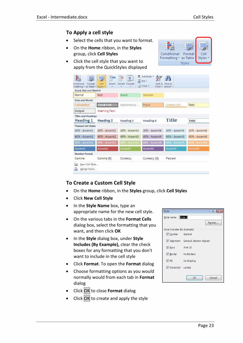
To Apply a cell style

Select the cells that you want to format.

On the Home ribbon, in the Styles group, click Cell Styles

Click the cell style that you want to apply from the QuickStyles displayed

To Create a Custom Cell Style

On the Home ribbon, in the Styles group, click Cell Styles

Click New Cell Style

In the Style Name box, type an appropriate name for the new cell style.

On the various tabs in the Format Cells dialog box, select the formatting that you want, and then click OK

In the Style dialog box, under Style Includes (By Example), clear the check boxes for any formatting that you don't want to include in the cell style

Click Format. To open the Format dialog

Choose formatting options as you would normally would from each tab in Format dialog

Click OK to close Format dialog

Click OK to create and apply the style

Cell Styles Excel - Intermediate.docx

Page 24

To remove a cell style

On the Home ribbon, in the Styles group, click Cell Styles.

To remove the cell style from the selected cells without deleting the cell style, choose the normal style this will remove all formatting from the cell,

To delete a created cell style the access the QuickStyles list.

Right click on desired cell style, choose delete.

You cannot delete the Normal cell style

Excel - Intermediate.docx Group and Ungroup Rows and Columns

Page 25

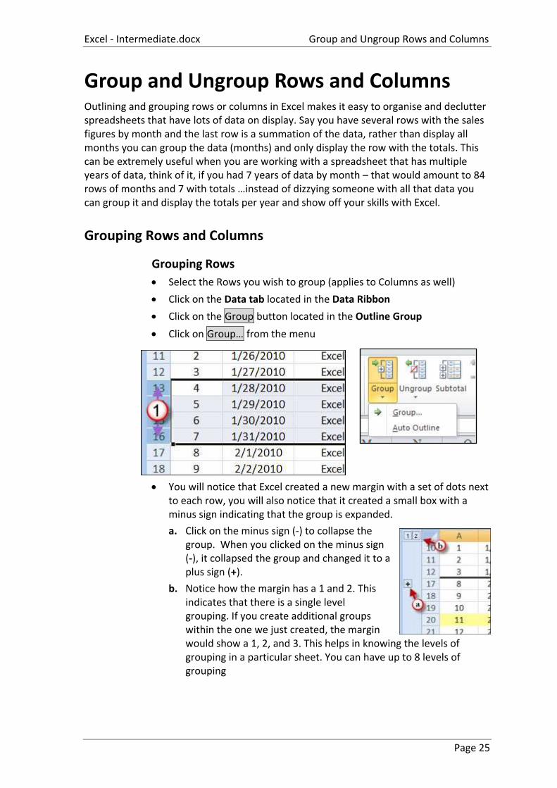
Group and Ungroup Rows and Columns Outlining and grouping rows or columns in Excel makes it easy to organise and declutter spreadsheets that have lots of data on display. Say you have several rows with the sales figures by month and the last row is a summation of the data, rather than display all months you can group the data (months) and only display the row with the totals. This can be extremely useful when you are working with a spreadsheet that has multiple years of data, think of it, if you had 7 years of data by month – that would amount to 84 rows of months and 7 with totals …instead of dizzying someone with all that data you can group it and display the totals per year and show off your skills with Excel.

Grouping Rows and Columns

Grouping Rows

Select the Rows you wish to group (applies to Columns as well)

Click on the Data tab located in the Data Ribbon

Click on the Group button located in the Outline Group

Click on Group… from the menu

You will notice that Excel created a new margin with a set of dots next to each row, you will also notice that it created a small box with a minus sign indicating that the group is expanded.

a. Click on the minus sign (-) to collapse the group. When you clicked on the minus sign (-), it collapsed the group and changed it to a plus sign (+).

b. Notice how the margin has a 1 and 2. This indicates that there is a single level grouping. If you create additional groups within the one we just created, the margin would show a 1, 2, and 3. This helps in knowing the levels of grouping in a particular sheet. You can have up to 8 levels of grouping

Group and Ungroup Rows and Columns Excel - Intermediate.docx

Page 26

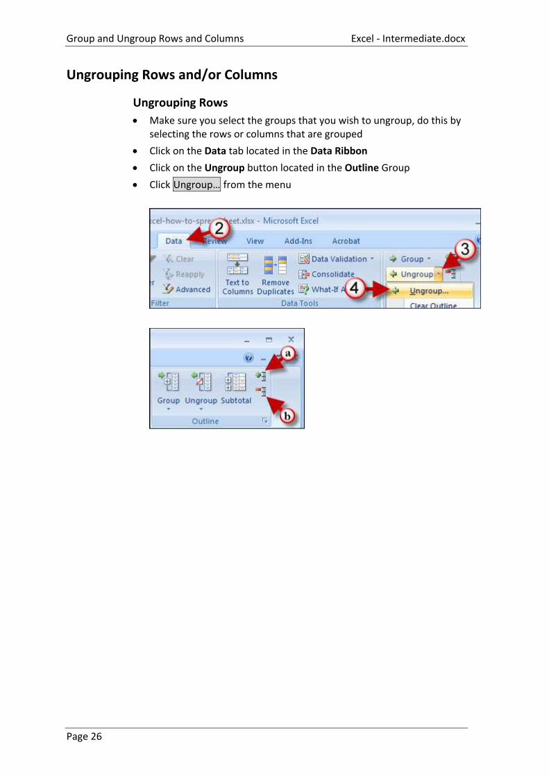
Ungrouping Rows and/or Columns

Ungrouping Rows

Make sure you select the groups that you wish to ungroup, do this by selecting the rows or columns that are grouped

Click on the Data tab located in the Data Ribbon

Click on the Ungroup button located in the Outline Group

Click Ungroup… from the menu

Excel - Intermediate.docx Protect Worksheet Data

Page 27

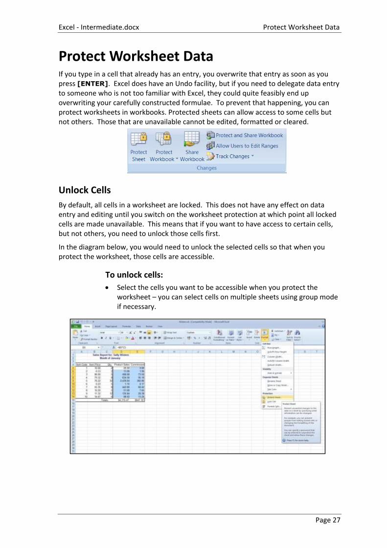
Protect Worksheet Data If you type in a cell that already has an entry, you overwrite that entry as soon as you press [ENTER]. Excel does have an Undo facility, but if you need to delegate data entry to someone who is not too familiar with Excel, they could quite feasibly end up overwriting your carefully constructed formulae. To prevent that happening, you can protect worksheets in workbooks. Protected sheets can allow access to some cells but not others. Those that are unavailable cannot be edited, formatted or cleared.

Unlock Cells

By default, all cells in a worksheet are locked. This does not have any effect on data entry and editing until you switch on the worksheet protection at which point all locked cells are made unavailable. This means that if you want to have access to certain cells, but not others, you need to unlock those cells first.

In the diagram below, you would need to unlock the selected cells so that when you protect the worksheet, those cells are accessible.

To unlock cells:

Select the cells you want to be accessible when you protect the worksheet – you can select cells on multiple sheets using group mode if necessary.

Protect Worksheet Data Excel - Intermediate.docx

Page 28

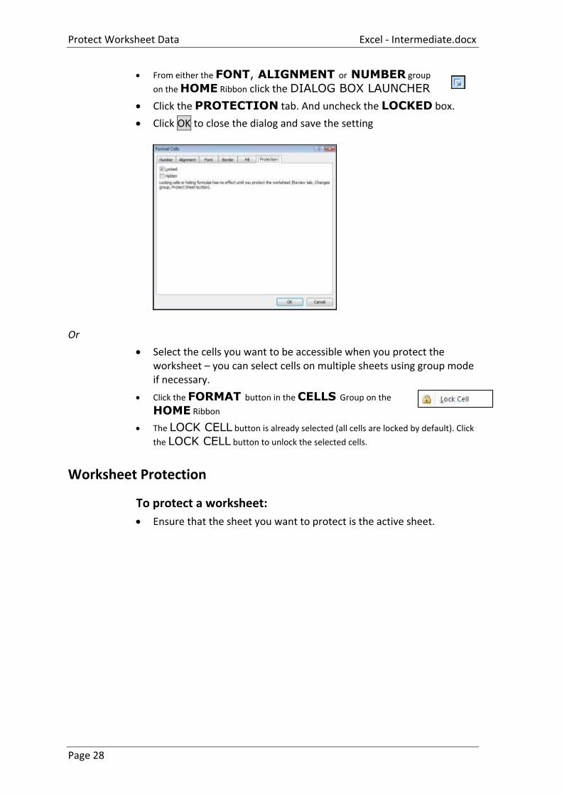
From either the FONT, ALIGNMENT or NUMBER group

on the HOME Ribbon click the DIALOG BOX LAUNCHER

Click the PROTECTION tab. And uncheck the LOCKED box.

Click OK to close the dialog and save the setting

Or

Select the cells you want to be accessible when you protect the worksheet – you can select cells on multiple sheets using group mode if necessary.

Click the FORMAT button in the CELLS Group on the

HOME Ribbon

The LOCK CELL button is already selected (all cells are locked by default). Click

the LOCK CELL button to unlock the selected cells.

Worksheet Protection

To protect a worksheet:

Ensure that the sheet you want to protect is the active sheet.

Excel - Intermediate.docx Protect Worksheet Data

Page 29

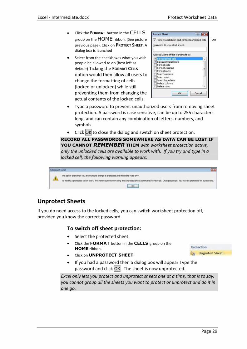
Click the FORMAT button in the CELLS

group on the HOME ribbon. (See picture on

previous page). Click on PROTECT SHEET. A

dialog box is launched

Select from the checkboxes what you wish people be allowed to do (best left as

default) Ticking the FORMAT CELLS option would then allow all users to change the formatting of cells (locked or unlocked) while still preventing them from changing the actual contents of the locked cells.

Type a password to prevent unauthorized users from removing sheet protection. A password is case sensitive, can be up to 255 characters long, and can contain any combination of letters, numbers, and symbols.

Click OK to close the dialog and switch on sheet protection.

RECORD ALL PASSWORDS SOMEWHERE AS DATA CAN BE LOST IF

YOU CANNOT REMEMBER THEM with worksheet protection active, only the unlocked cells are available to work with. If you try and type in a locked cell, the following warning appears:

Unprotect Sheets

If you do need access to the locked cells, you can switch worksheet protection off, provided you know the correct password.

To switch off sheet protection:

Select the protected sheet.

Click the FORMAT button in the CELLS group on the

HOME ribbon.

Click on UNPROTECT SHEET.

If you had a password then a dialog box will appear Type the

password and click OK. The sheet is now unprotected.

Excel only lets you protect and unprotect sheets one at a time, that is to say, you cannot group all the sheets you want to protect or unprotect and do it in one go.

Protect Worksheet Data Excel - Intermediate.docx

Page 30

Making your File Read Only

Creating a Read Only File:

If your Excel file has important information and you do not want the file to be edited then you may make the file as a read-only file. Perform the following steps to do so:

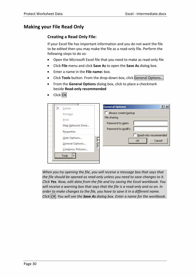
Open the Microsoft Excel file that you need to make as read-only file

Click File menu and click Save As to open the Save As dialog box.

Enter a name in the File name: box.

Click Tools button. From the drop-down box, click General Options…

From the General Options dialog box, click to place a checkmark beside Read-only recommended

Click OK

When you try opening the file, you will receive a message box that says that the file should be opened as read-only unless you need to save changes to it. Click Yes. Now, edit data from the file and try saving the Excel workbook. You will receive a warning box that says that the file is a read-only and so on. In order to make changes to the file, you have to save it in a different name.

Click OK. You will see the Save As dialog box. Enter a name for the workbook.

Excel - Intermediate.docx Data Validation Rules

Page 31

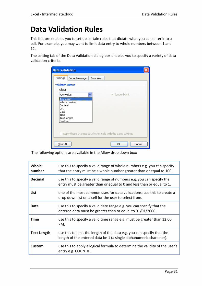
Data Validation Rules This feature enables you to set up certain rules that dictate what you can enter into a cell. For example, you may want to limit data entry to whole numbers between 1 and 12.

The setting tab of the Data Validation dialog box enables you to specify a variety of data validation criteria.

The following options are available in the Allow drop down box:

Whole number

use this to specify a valid range of whole numbers e.g. you can specify that the entry must be a whole number greater than or equal to 100.

Decimal use this to specify a valid range of numbers e.g. you can specify the entry must be greater than or equal to 0 and less than or equal to 1.

List one of the most common uses for data validations; use this to create a drop down list on a cell for the user to select from.

Date use this to specify a valid date range e.g. you can specify that the entered data must be greater than or equal to 01/01/2000.

Time use this to specify a valid time range e.g. must be greater than 12:00 PM.

Text Length use this to limit the length of the data e.g. you can specify that the length of the entered data be 1 (a single alphanumeric character).

Custom use this to apply a logical formula to determine the validity of the user’s entry e.g. COUNTIF.

Data Validation Rules Excel - Intermediate.docx

Page 32

Setting Validation Rules

Creating a data validation on a worksheet

Select the cell or range to validate.

On the Data Ribbon, select Data Validation from the Data Tools

group and then click the Settings tab

Specify the type of validation you want (using one of the options above), in the validation criteria.

Set the Validation Data i.e. Minimum and Maximum.

Note: setting the Ignore blank check box allows any values to be entered in the validated cell. This is also true for any cells referenced by validation formulas: if any referenced cell is blank, setting the Ignore blank check box allows any values to be entered in the validated cell.

To display an optional input message when the cell is clicked, click the Input Message tab, and make sure the Show input message when cell is selected check box is selected, and fill in the title and text for the message.

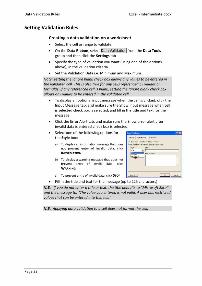
Click the Error Alert tab, and make sure the Show error alert after invalid data is entered check box is selected.

Select one of the following options for the Style box:

a) To display an information message that does not prevent entry of invalid data, click

INFORMATION

b) To display a warning message that does not prevent entry of invalid data, click

WARNING

c) To prevent entry of invalid data, click STOP

Fill in the title and text for the message (up to 225 characters)

N.B. If you do not enter a title or text, the title defaults to "Microsoft Excel" and the message to: "The value you entered is not valid. A user has restricted values that can be entered into this cell."

N.B. Applying data validation to a cell does not format the cell.

Excel - Intermediate.docx Track Changes

Page 33

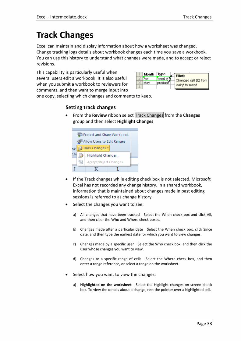
Track Changes Excel can maintain and display information about how a worksheet was changed. Change tracking logs details about workbook changes each time you save a workbook. You can use this history to understand what changes were made, and to accept or reject revisions.

This capability is particularly useful when several users edit a workbook. It is also useful when you submit a workbook to reviewers for comments, and then want to merge input into one copy, selecting which changes and comments to keep.

Setting track changes

From the Review ribbon select Track Changes from the Changes

group and then select Highlight Changes

If the Track changes while editing check box is not selected, Microsoft Excel has not recorded any change history. In a shared workbook, information that is maintained about changes made in past editing sessions is referred to as change history.

Select the changes you want to see:

a) All changes that have been tracked Select the When check box and click All, and then clear the Who and Where check boxes.

b) Changes made after a particular date Select the When check box, click Since date, and then type the earliest date for which you want to view changes.

c) Changes made by a specific user Select the Who check box, and then click the user whose changes you want to view.

d) Changes to a specific range of cells Select the Where check box, and then enter a range reference, or select a range on the worksheet.

Select how you want to view the changes:

a) Highlighted on the worksheet Select the Highlight changes on screen check box. To view the details about a change, rest the pointer over a highlighted cell.

Track Changes Excel - Intermediate.docx

Page 34

b) Listed on a separate sheet Select the List changes on a new sheet check box to display the History worksheet. This check box is available only after you've turned on change tracking and saved some changes.

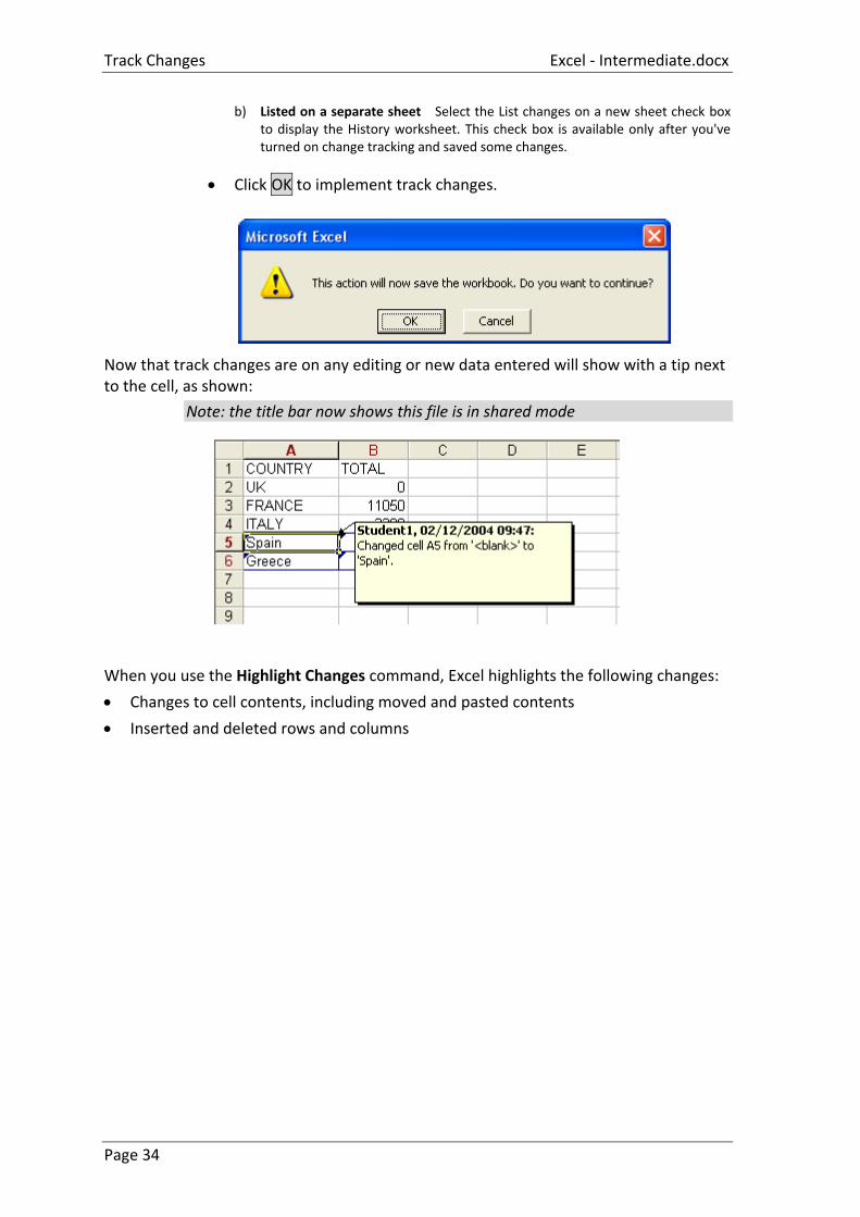
Click OK to implement track changes.

Now that track changes are on any editing or new data entered will show with a tip next to the cell, as shown:

Note: the title bar now shows this file is in shared mode

When you use the Highlight Changes command, Excel highlights the following changes:

Changes to cell contents, including moved and pasted contents

Inserted and deleted rows and columns

Excel - Intermediate.docx Track Changes

Page 35

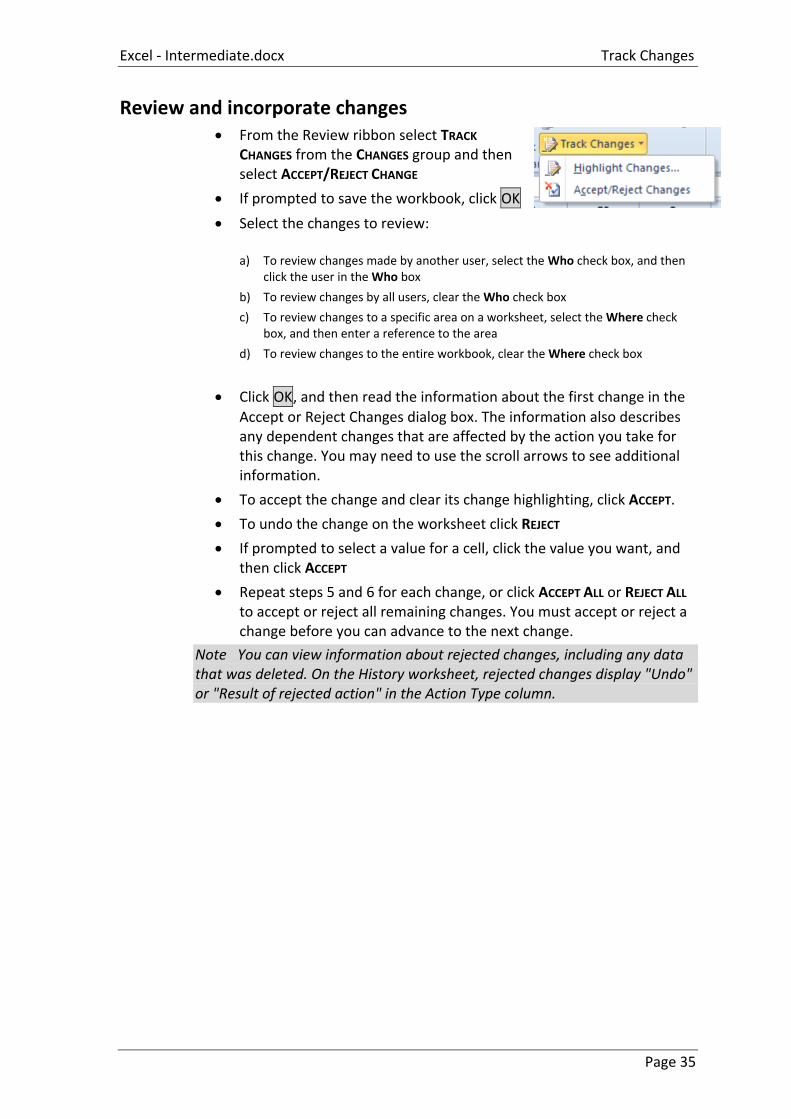
Review and incorporate changes From the Review ribbon select TRACK

CHANGES from the CHANGES group and then select ACCEPT/REJECT CHANGE

If prompted to save the workbook, click OK

Select the changes to review: a) To review changes made by another user, select the Who check box, and then

click the user in the Who box

b) To review changes by all users, clear the Who check box

c) To review changes to a specific area on a worksheet, select the Where check box, and then enter a reference to the area

d) To review changes to the entire workbook, clear the Where check box

Click OK, and then read the information about the first change in the

Accept or Reject Changes dialog box. The information also describes any dependent changes that are affected by the action you take for this change. You may need to use the scroll arrows to see additional information.

To accept the change and clear its change highlighting, click ACCEPT.

To undo the change on the worksheet click REJECT

If prompted to select a value for a cell, click the value you want, and then click ACCEPT

Repeat steps 5 and 6 for each change, or click ACCEPT ALL or REJECT ALL to accept or reject all remaining changes. You must accept or reject a change before you can advance to the next change.

Note You can view information about rejected changes, including any data that was deleted. On the History worksheet, rejected changes display "Undo" or "Result of rejected action" in the Action Type column.

What-If Analysis Excel - Intermediate.docx

Page 36

What-If Analysis Excel has a number of ways of altering conditions on the spreadsheet and making formulae produce whatever result is requested. Excel can also forecast what conditions on the spreadsheet would be needed to optimise the result of a formula. For instance, there may be a profits figure that needs to be kept as high as possible, a costs figure that needs to be kept to a minimum, or a budget constraint that has to equal a certain figure exactly. Usually, these figures are formulae that depend on a great many other variables on the spreadsheet. Therefore, you would have to do an awful lot of trial-and-error analysis to obtain the desired result. Excel can, however, perform this analysis very quickly to obtain optimum results. The Goal Seek command can be used to make a formula achieve a certain value by altering just one variable. The Solver can be used for more painstaking analysis where many variables could be adjusted to reach a desired result. The Solver can be used to not only obtain a specific value, but also to maximise or minimise the result of a formula (e.g. maximise profits or minimise costs).

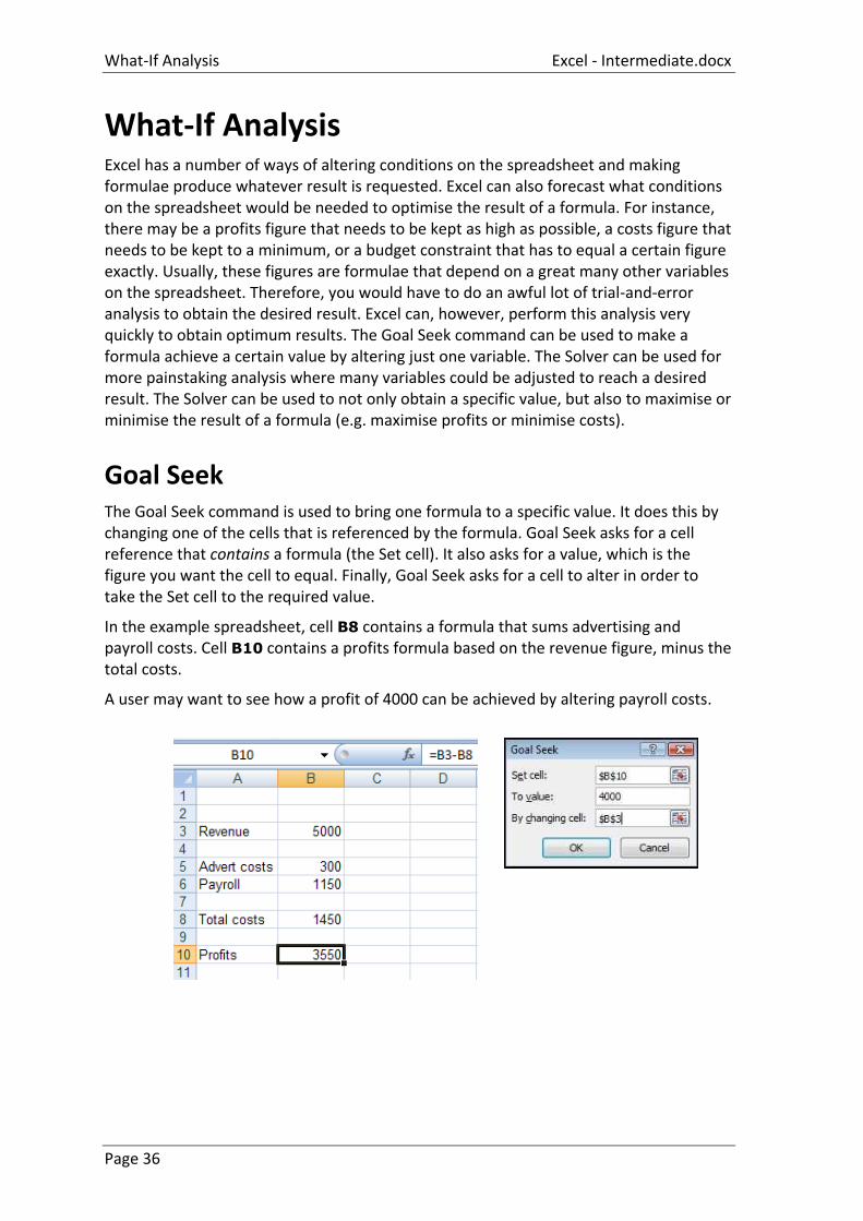
Goal Seek The Goal Seek command is used to bring one formula to a specific value. It does this by changing one of the cells that is referenced by the formula. Goal Seek asks for a cell reference that contains a formula (the Set cell). It also asks for a value, which is the figure you want the cell to equal. Finally, Goal Seek asks for a cell to alter in order to take the Set cell to the required value.

In the example spreadsheet, cell B8 contains a formula that sums advertising and payroll costs. Cell B10 contains a profits formula based on the revenue figure, minus the total costs.

A user may want to see how a profit of 4000 can be achieved by altering payroll costs.

Excel - Intermediate.docx What-If Analysis

Page 37

To launch the Goal Seeker:

On the DATA ribbon, DATA TOOLS group, click WHAT-IF

ANALYSIS and then click GOAL SEEK.

In the SET CELL box, enter the reference for the cell that contains the formula result you wish to set to a specific figure. (In the example, this is cell B10.)

In the TO VALUE box, type the result you want. (In the example, this is -4000.)

In the BY CHANGING CELL box, enter the reference for the cell that contains the value you want to adjust. (In the example, this is cell B3.)

The Goal Seek command automatically suggests the active cell as the Set cell. This can be overtyped with a new cell reference or you may click on the appropriate cell on the spreadsheet.

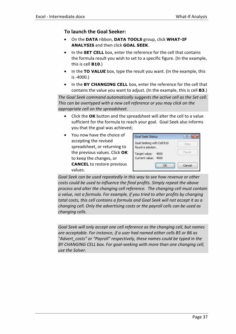
Click the OK button and the spreadsheet will alter the cell to a value sufficient for the formula to reach your goal. Goal Seek also informs you that the goal was achieved;

You now have the choice of accepting the revised spreadsheet, or returning to the previous values. Click OK to keep the changes, or CANCEL to restore previous values.

Goal Seek can be used repeatedly in this way to see how revenue or other costs could be used to influence the final profits. Simply repeat the above process and alter the changing cell reference. The changing cell must contain a value, not a formula. For example, if you tried to alter profits by changing total costs, this cell contains a formula and Goal Seek will not accept it as a changing cell. Only the advertising costs or the payroll cells can be used as changing cells.

Goal Seek will only accept one cell reference as the changing cell, but names are acceptable. For instance, if a user had named either cells B5 or B6 as "Advert_costs" or "Payroll" respectively, these names could be typed in the BY CHANGING CELL box. For goal-seeking with more than one changing cell, use the Solver.

Solver Excel - Intermediate.docx

Page 38

Solver For more complex trial-and-error analysis the Excel Solver should be used. Unlike Goal Seek, the Solver can alter a formula not just to produce a set value, but also to maximise or minimise the result. Solver has changed markedly in 2010 from previous versions but works in very much the same way. More than one changing cell can be specified, so as to increase the number of possibilities, and constraints can be built in to restrict the analysis to operate only under specific conditions.

The basis for using the Solver is usually to alter many figures to produce the optimum result for a single formula. This could mean, for example, altering price figures to maximise profits. It could mean adjusting expenditure to minimise costs, etc. Whatever the case, the variable figures to be adjusted must have an influence, either, directly or indirectly, on the overall result, that is to say the changing cells must affect the formula to be optimised. Up to 200 changing cells can be included in the solving process, and up to 100 constraints can be built in to limit the Solver's results.

Solver Parameters

The Solver needs quite a lot of information in order for it to be able to come up with a realistic solution. These are the Solver parameters

To set up the Solver:

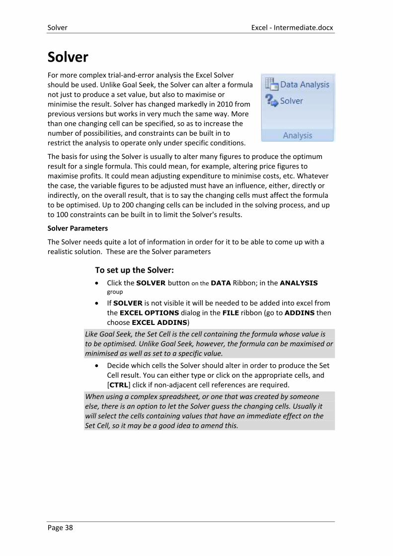
Click the SOLVER button on the DATA Ribbon; in the ANALYSIS

group

If SOLVER is not visible it will be needed to be added into excel from the EXCEL OPTIONS dialog in the FILE ribbon (go to ADDINS then choose EXCEL ADDINS)

Like Goal Seek, the Set Cell is the cell containing the formula whose value is to be optimised. Unlike Goal Seek, however, the formula can be maximised or minimised as well as set to a specific value.

Decide which cells the Solver should alter in order to produce the Set Cell result. You can either type or click on the appropriate cells, and [CTRL] click if non-adjacent cell references are required.

When using a complex spreadsheet, or one that was created by someone else, there is an option to let the Solver guess the changing cells. Usually it will select the cells containing values that have an immediate effect on the Set Cell, so it may be a good idea to amend this.

Excel - Intermediate.docx Solver

Page 39

Constraints

Constraints prevent the Solver from coming up with unrealistic solutions.

To build constraints into your Solver parameters:

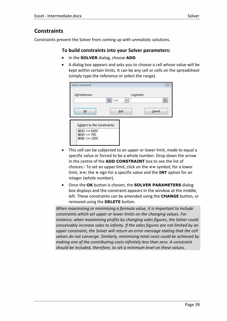
In the SOLVER dialog, choose ADD

A dialog box appears and asks you to choose a cell whose value will be kept within certain limits. It can be any cell or cells on the spreadsheet (simply type the reference or select the range).

This cell can be subjected to an upper or lower limit, made to equal a specific value or forced to be a whole number. Drop down the arrow in the centre of the ADD CONSTRAINT box to see the list of choices:- To set an upper limit, click on the <= symbol; for a lower limit, >=; the = sign for a specific value and the INT option for an integer (whole number).

Once the OK button is chosen, the SOLVER PARAMETERS dialog box displays and the constraint appears in the window at the middle, left. These constraints can be amended using the CHANGE button, or removed using the DELETE button.

When maximising or minimising a formula value, it is important to include constraints which set upper or lower limits on the changing values. For instance, when maximising profits by changing sales figures, the Solver could conceivably increase sales to infinity. If the sales figures are not limited by an upper constraint, the Solver will return an error message stating that the cell values do not converge. Similarly, minimising total costs could be achieved by making one of the contributing costs infinitely less than zero. A constraint should be included, therefore, to set a minimum level on these values.


Page 40

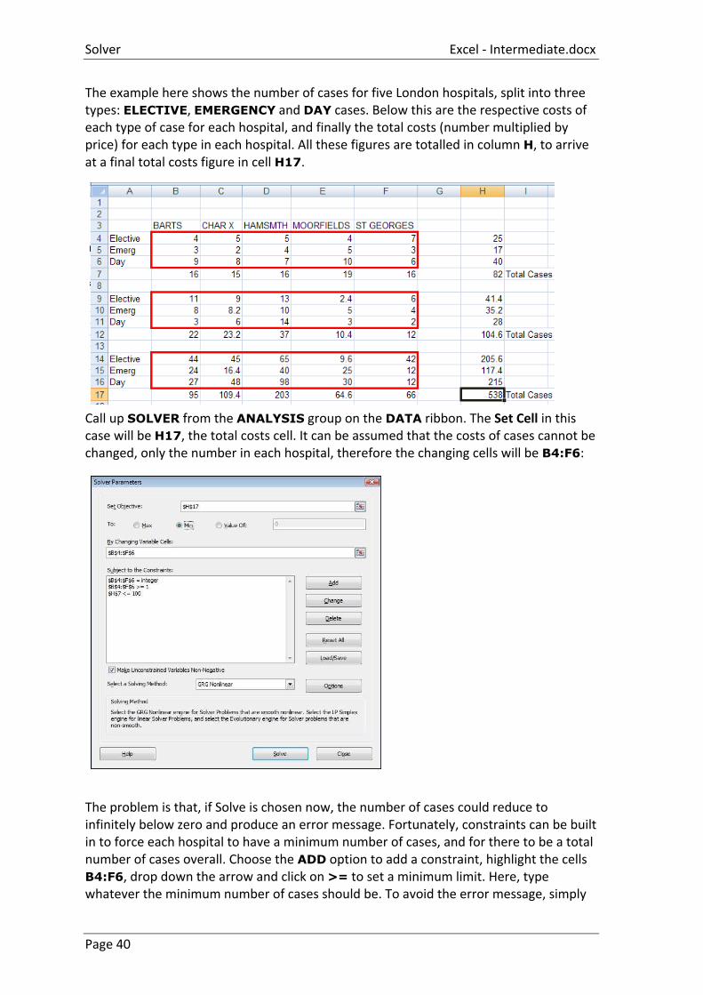
The example here shows the number of cases for five London hospitals, split into three types: ELECTIVE, EMERGENCY and DAY cases. Below this are the respective costs of each type of case for each hospital, and finally the total costs (number multiplied by price) for each type in each hospital. All these figures are totalled in column H, to arrive at a final total costs figure in cell H17.

Call up SOLVER from the ANALYSIS group on the DATA ribbon. The Set Cell in this case will be H17, the total costs cell. It can be assumed that the costs of cases cannot be changed, only the number in each hospital, therefore the changing cells will be B4:F6:

The problem is that, if Solve is chosen now, the number of cases could reduce to infinitely below zero and produce an error message. Fortunately, constraints can be built in to force each hospital to have a minimum number of cases, and for there to be a total number of cases overall. Choose the ADD option to add a constraint, highlight the cells B4:F6, drop down the arrow and click on >= to set a minimum limit. Here, type whatever the minimum number of cases should be. To avoid the error message, simply


Page 41

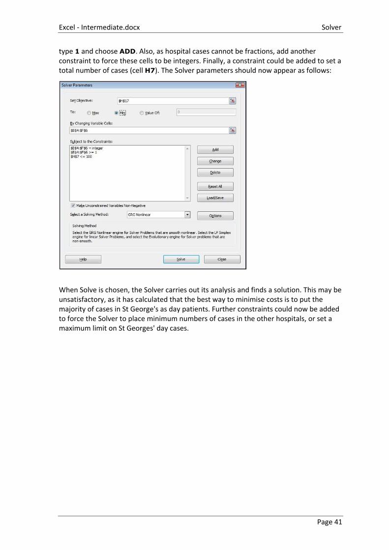
type 1 and choose ADD. Also, as hospital cases cannot be fractions, add another constraint to force these cells to be integers. Finally, a constraint could be added to set a total number of cases (cell H7). The Solver parameters should now appear as follows:

When Solve is chosen, the Solver carries out its analysis and finds a solution. This may be unsatisfactory, as it has calculated that the best way to minimise costs is to put the majority of cases in St George's as day patients. Further constraints could now be added to force the Solver to place minimum numbers of cases in the other hospitals, or set a maximum limit on St Georges' day cases.


Page 42

Advanced Solver Features

Save or Load A Problem Model:

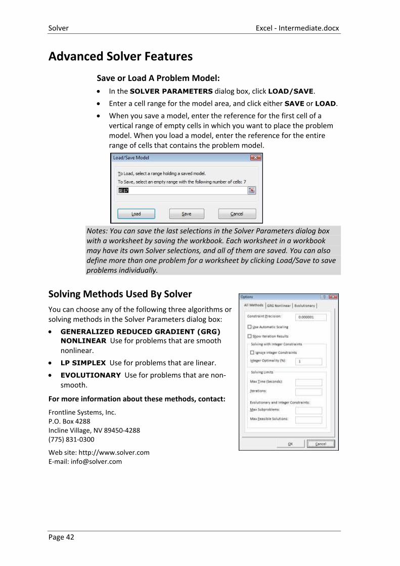
In the SOLVER PARAMETERS dialog box, click LOAD/SAVE.

Enter a cell range for the model area, and click either SAVE or LOAD.

When you save a model, enter the reference for the first cell of a vertical range of empty cells in which you want to place the problem model. When you load a model, enter the reference for the entire range of cells that contains the problem model.

Notes: You can save the last selections in the Solver Parameters dialog box with a worksheet by saving the workbook. Each worksheet in a workbook may have its own Solver selections, and all of them are saved. You can also define more than one problem for a worksheet by clicking Load/Save to save problems individually.

Solving Methods Used By Solver

You can choose any of the following three algorithms or solving methods in the Solver Parameters dialog box:

GENERALIZED REDUCED GRADIENT (GRG)

NONLINEAR Use for problems that are smooth nonlinear.

LP SIMPLEX Use for problems that are linear.

EVOLUTIONARY Use for problems that are non-smooth.

For more information about these methods, contact:

Frontline Systems, Inc. P.O. Box 4288 Incline Village, NV 89450-4288 (775) 831-0300

Web site: http://www.solver.com E-mail: [email protected]


Page 43

Solver Options

There are many options that you can access to refine your results for each of the solving methods mentioned above access these by clicking on the OPTIONS button on the SOLVER PARAMETERS dialog

Solver and Scenario Manager

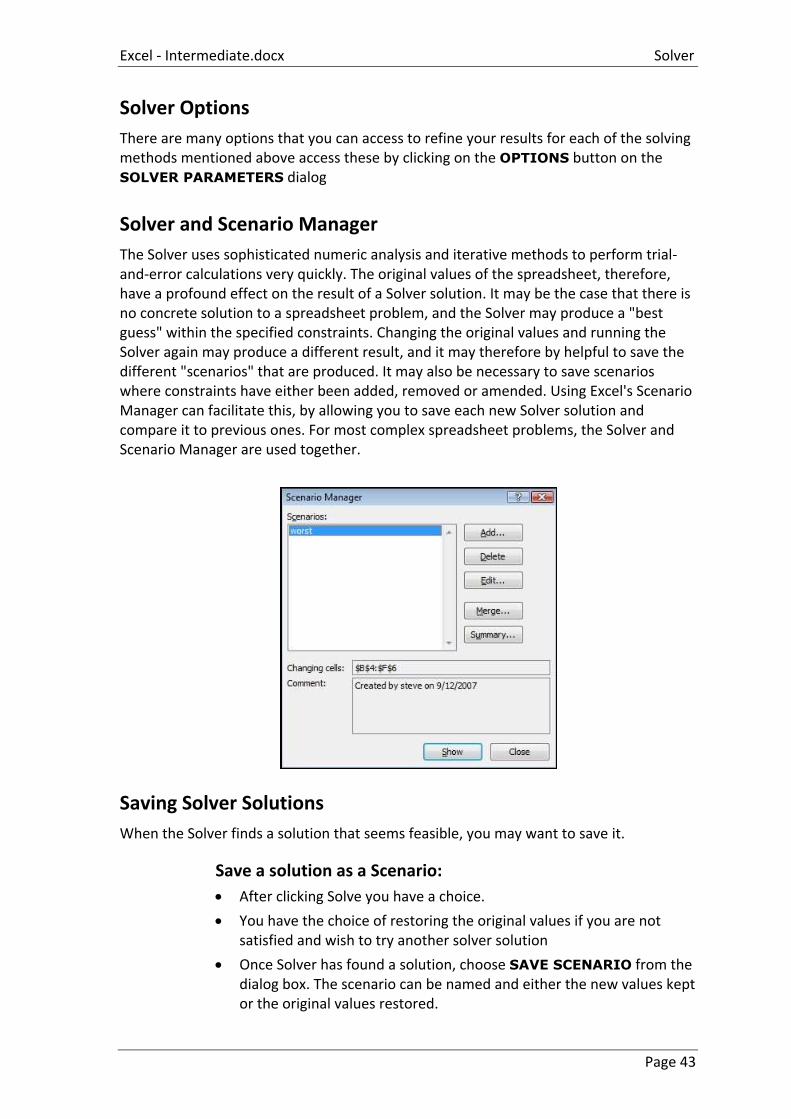
The Solver uses sophisticated numeric analysis and iterative methods to perform trial-and-error calculations very quickly. The original values of the spreadsheet, therefore, have a profound effect on the result of a Solver solution. It may be the case that there is no concrete solution to a spreadsheet problem, and the Solver may produce a "best guess" within the specified constraints. Changing the original values and running the Solver again may produce a different result, and it may therefore by helpful to save the different "scenarios" that are produced. It may also be necessary to save scenarios where constraints have either been added, removed or amended. Using Excel's Scenario Manager can facilitate this, by allowing you to save each new Solver solution and compare it to previous ones. For most complex spreadsheet problems, the Solver and Scenario Manager are used together.

Saving Solver Solutions

When the Solver finds a solution that seems feasible, you may want to save it.

Save a solution as a Scenario:

After clicking Solve you have a choice.

You have the choice of restoring the original values if you are not satisfied and wish to try another solver solution

Once Solver has found a solution, choose SAVE SCENARIO from the dialog box. The scenario can be named and either the new values kept or the original values restored.


Page 44

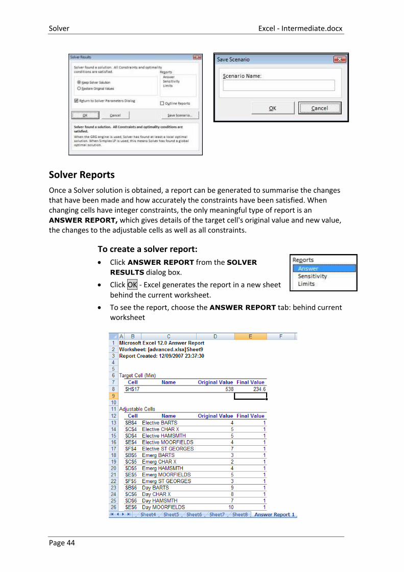
Solver Reports

Once a Solver solution is obtained, a report can be generated to summarise the changes that have been made and how accurately the constraints have been satisfied. When changing cells have integer constraints, the only meaningful type of report is an ANSWER REPORT, which gives details of the target cell's original value and new value, the changes to the adjustable cells as well as all constraints.

To create a solver report:

Click ANSWER REPORT from the SOLVER

RESULTS dialog box.

Click OK - Excel generates the report in a new sheet

behind the current worksheet.

To see the report, choose the ANSWER REPORT tab: behind current worksheet


Page 45

Scenario Manager

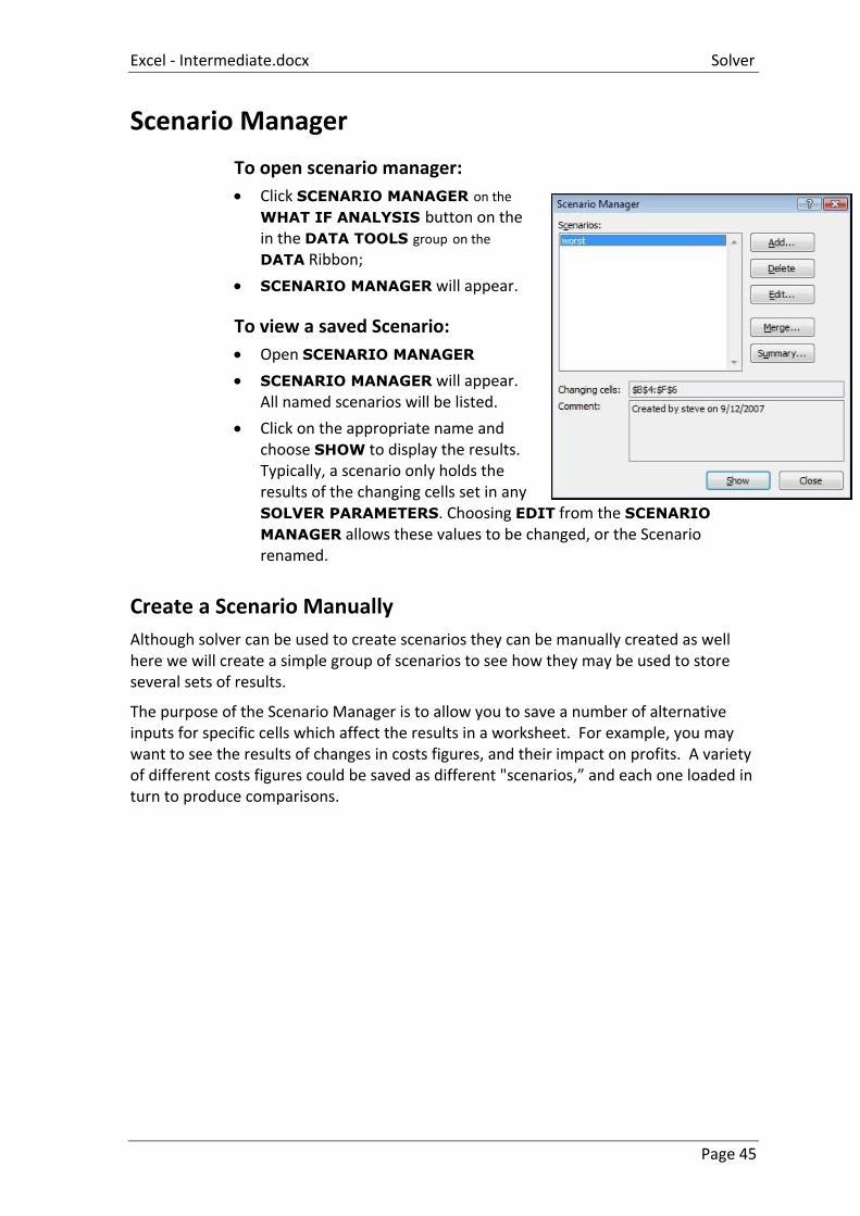
To open scenario manager:

Click SCENARIO MANAGER on the

WHAT IF ANALYSIS button on the in the DATA TOOLS group on the DATA Ribbon;

SCENARIO MANAGER will appear.

To view a saved Scenario:

Open SCENARIO MANAGER

SCENARIO MANAGER will appear. All named scenarios will be listed.

Click on the appropriate name and choose SHOW to display the results. Typically, a scenario only holds the results of the changing cells set in any SOLVER PARAMETERS. Choosing EDIT from the SCENARIO

MANAGER allows these values to be changed, or the Scenario renamed.

Create a Scenario Manually

Although solver can be used to create scenarios they can be manually created as well here we will create a simple group of scenarios to see how they may be used to store several sets of results.

The purpose of the Scenario Manager is to allow you to save a number of alternative inputs for specific cells which affect the results in a worksheet. For example, you may want to see the results of changes in costs figures, and their impact on profits. A variety of different costs figures could be saved as different "scenarios,” and each one loaded in turn to produce comparisons.


Page 46

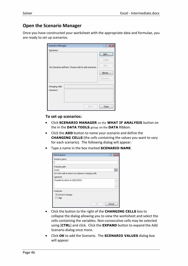
Open the Scenario Manager

Once you have constructed your worksheet with the appropriate data and formulae, you are ready to set up scenarios.

To set up scenarios:

Click SCENARIO MANAGER on the WHAT IF ANALYSIS button on the in the DATA TOOLS group on the DATA Ribbon.

Click the ADD button to name your scenario and define the CHANGING CELLS (the cells containing the values you want to vary for each scenario). The following dialog will appear:

Type a name in the box marked SCENARIO NAME.

Click the button to the right of the CHANGING CELLS box to collapse the dialog allowing you to view the worksheet and select the cells containing the variables. Non-consecutive cells may be selected using [CTRL] and click. Click the EXPAND button to expand the Add Scenario dialog once more.

Click OK to add the Scenario. The SCENARIO VALUES dialog box will appear:


Page 47

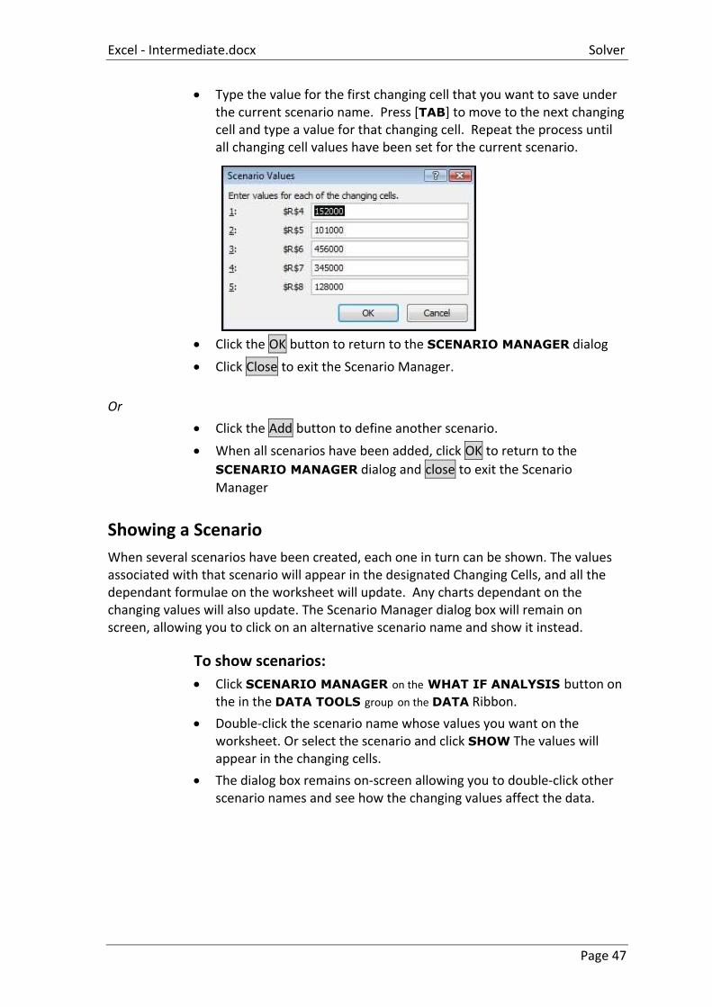
Type the value for the first changing cell that you want to save under the current scenario name. Press [TAB] to move to the next changing cell and type a value for that changing cell. Repeat the process until all changing cell values have been set for the current scenario.

Click the OK button to return to the SCENARIO MANAGER dialog

Click Close to exit the Scenario Manager.

Or

Click the Add button to define another scenario.

When all scenarios have been added, click OK to return to the

SCENARIO MANAGER dialog and close to exit the Scenario

Manager

Showing a Scenario

When several scenarios have been created, each one in turn can be shown. The values associated with that scenario will appear in the designated Changing Cells, and all the dependant formulae on the worksheet will update. Any charts dependant on the changing values will also update. The Scenario Manager dialog box will remain on screen, allowing you to click on an alternative scenario name and show it instead.

To show scenarios:

Click SCENARIO MANAGER on the WHAT IF ANALYSIS button on the in the DATA TOOLS group on the DATA Ribbon.

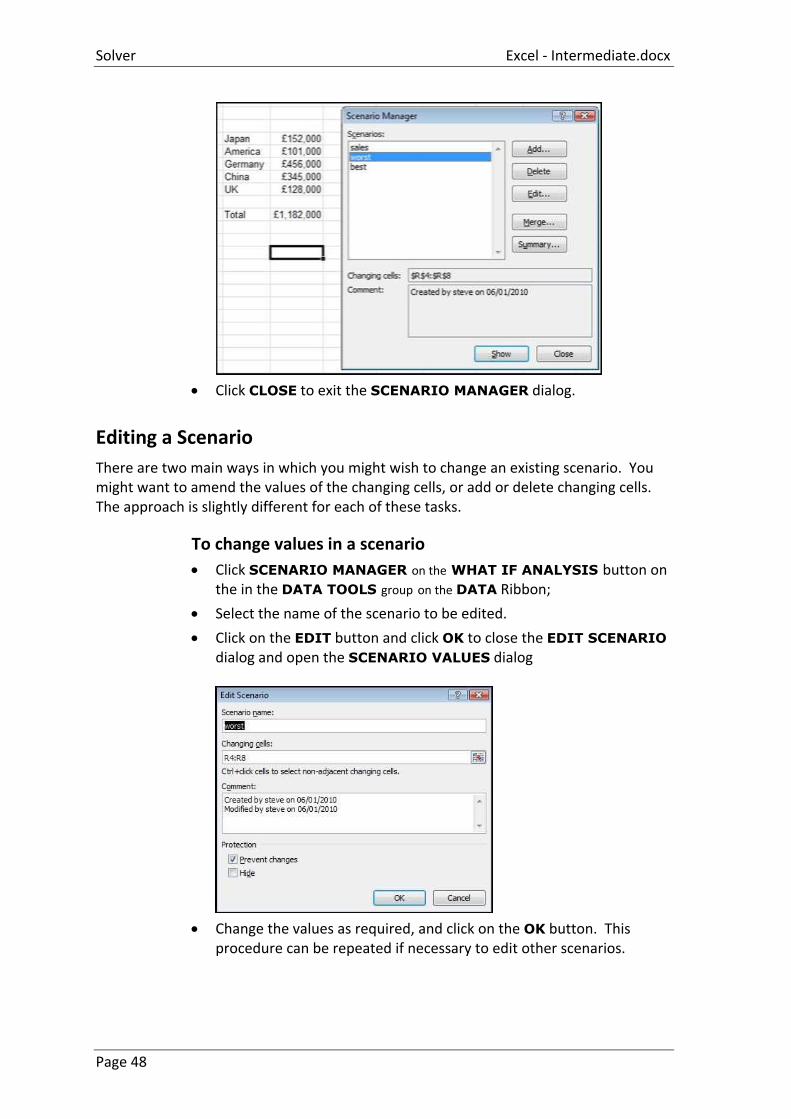
Double-click the scenario name whose values you want on the worksheet. Or select the scenario and click SHOW The values will appear in the changing cells.

The dialog box remains on-screen allowing you to double-click other scenario names and see how the changing values affect the data.


Page 48

Click CLOSE to exit the SCENARIO MANAGER dialog.

Editing a Scenario

There are two main ways in which you might wish to change an existing scenario. You might want to amend the values of the changing cells, or add or delete changing cells. The approach is slightly different for each of these tasks.

To change values in a scenario

Click SCENARIO MANAGER on the WHAT IF ANALYSIS button on the in the DATA TOOLS group on the DATA Ribbon;

Select the name of the scenario to be edited.

Click on the EDIT button and click OK to close the EDIT SCENARIO dialog and open the SCENARIO VALUES dialog

Change the values as required, and click on the OK button. This procedure can be repeated if necessary to edit other scenarios.


Page 49

To add changing cells:

Click SCENARIO MANAGER on the WHAT IF ANALYSIS button on the in the DATA TOOLS group on the DATA Ribbon; (


Click on the EDIT button and click the button to the right of the CHANGING CELLS box to collapse the EDIT SCENARIO dialog.

Hold down the [CTRL] key as you click and drag across the cells that you want to add. Click the button to expand the dialog. Click OK to confirm the addition.

Enter the value for the newly added changing cell in the SCENARIO

VALUES dialog and click OK to confirm.

Click CLOSE to exit the Scenario Manager.

To remove changing cells:



Click on the EDIT button.

Drag across the cell references of the cells you want to remove from the CHANGING CELLS box and press [DELETE]. Click OK to confirm the deletion and OK again to close the SCENARIO VALUES dialog.

Click CLOSE to exit the Scenario Manager.

Deleting a Scenario

To delete a scenario:


Select the name of the scenario to be deleted.

1. There will be no prompt to confirm deletion when deleting a scenario so ensure you have the correct scenario selected.

2. Take note you can’t undo the deletion of a scenario.

Click Delete button. The scenario is removed


Page 50

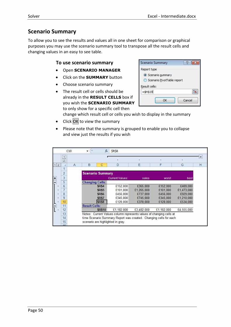
Scenario Summary

To allow you to see the results and values all in one sheet for comparison or graphical purposes you may use the scenario summary tool to transpose all the result cells and changing values in an easy to see table.

To use scenario summary

Open SCENARIO MANAGER

Click on the SUMMARY button

Choose scenario summary

The result cell or cells should be already in the RESULT CELLS box if you wish the SCENARIO SUMMARY to only show for a specific cell then change which result cell or cells you wish to display in the summary

Click OK to view the summary

Please note that the summary is grouped to enable you to collapse and view just the results if you wish

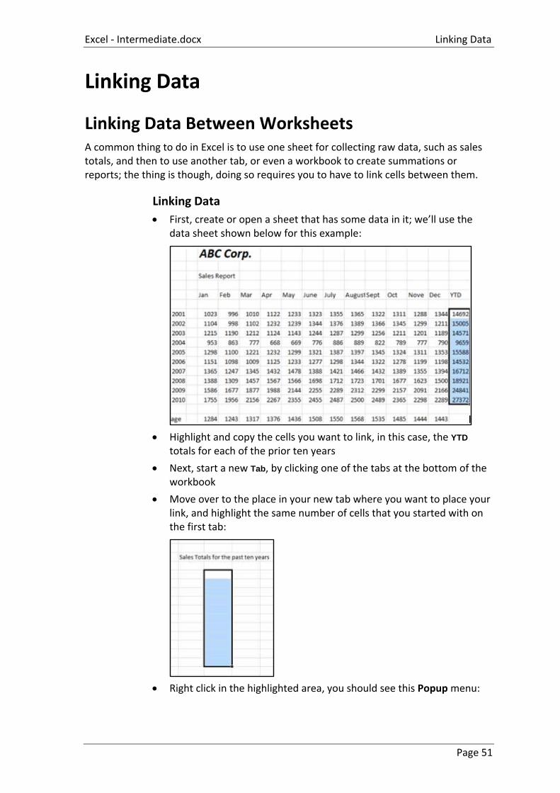
Excel - Intermediate.docx Linking Data

Page 51

Linking Data

Linking Data Between Worksheets A common thing to do in Excel is to use one sheet for collecting raw data, such as sales totals, and then to use another tab, or even a workbook to create summations or reports; the thing is though, doing so requires you to have to link cells between them.

Linking Data

First, create or open a sheet that has some data in it; we’ll use the data sheet shown below for this example:

Highlight and copy the cells you want to link, in this case, the YTD totals for each of the prior ten years

Next, start a new Tab, by clicking one of the tabs at the bottom of the workbook

Move over to the place in your new tab where you want to place your link, and highlight the same number of cells that you started with on the first tab:

Right click in the highlighted area, you should see this Popup menu:

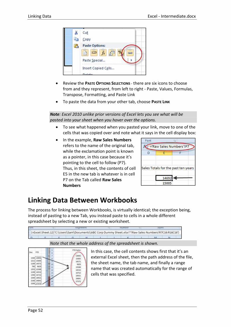
Linking Data Excel - Intermediate.docx

Page 52

Review the PASTE OPTIONS SELECTIONS - there are six icons to choose from and they represent, from left to right - Paste, Values, Formulas, Transpose, Formatting, and Paste Link

To paste the data from your other tab, choose PASTE LINK

Note: Excel 2010 unlike prior versions of Excel lets you see what will be pasted into your sheet when you hover over the options.

To see what happened when you pasted your link, move to one of the cells that was copied over and note what it says in the cell display box:

In the example, Raw Sales Numbers refers to the name of the original tab, while the exclamation point is known as a pointer, in this case because it’s pointing to the cell to follow (P7). Thus, in this sheet, the contents of cell E5 in the new tab is whatever is in cell P7 on the Tab called Raw Sales Numbers

Linking Data Between Workbooks The process for linking between Workbooks, is virtually identical; the exception being, instead of pasting to a new Tab, you instead paste to cells in a whole different spreadsheet by selecting a new or existing worksheet.

Note that the whole address of the spreadsheet is shown.

In this case, the cell contents shows first that it’s an external Excel sheet, then the path address of the file, the sheet name, the tab name, and finally a range name that was created automatically for the range of cells that was specified.

http://www.ficpa.org/Content/Files/Img/Sections/BizTech/techtips/2011/032411/5b.jpg

Documents

Microsoft Office 2010 Worksheets Excel - Intermediate.docx Page 2 Grouping Worksheets Activate Group Mode Whenever you select more than one worksheet, Excel considers those sheets