Embed Size (px)
Citation preview
Methods of Psychological Research Online 2003, Vol.8, No.2, pp. 75-112 Department of Psychology
Internet: http://www.mpr-online.de © 2003 University of Koblenz-Landau
Structural Equations Modeling in Developmental Research
Concepts and Applications1
Alexander von Eye2
Michigan State University
Christiane Spiel and Petra Wagner
University of Wien
This article discusses structural models for developmental research. First, it gives a
brief overview of structural modeling using the well-known LISREL notation. Then,
characteristics of well-fitting models are reviewed. These characteristics are presented
with the goal in mind of presenting complete reports of structural models such that
readers are enabled to derive their own conclusions concerning a model. The features
of developmental models are discussed. Models are developmental in particular when
some variation of time or age is central to the hypotheses under study. Data examples
are presented from a study on the long-term effects of biological and social risks in in-
fancy and early childhood. These examples suggest that performance in academic sub-
jects in school at age 11 can be predicted based on information of early risks. The
models are discussed with reference to the characteristics of well-fitting models.
Keywords: developmental modeling, fit criteria, developmental hypotheses, structural
modeling
The purpose of this article is to discuss and illustrate structural equations modeling
(SEM) for research in disciplines concerned with development, for example, develop-
mental psychology, education, or developmental psychopathology. This article provides
an overview of SEM concepts and methods, and presents examples, using data from a
1 This research was in part supported by the Austrian “Fonds zur Förderung der wissenschaftlichen For-
schung” Grant No. P7630-SOZ and by the Johann Jacobs Foundation. 2 Correspondence concerning this article should be addressed to Alexander von Eye, Michigan State Uni-
versity, Department of Psychology, 119 Snyder Hall, East Lansing, MI 48824-1117, USA;
E-mail [email protected]
76 MPR-Online 2003, Vol. 8, No. 2
study on the prediction of performance in academic subjects in elementary school from
indicators of risk in early childhood.
We also discuss characteristics of well-fitting models. In this discussion, we posit that
models can be appreciated by readers only if they are described to the extent that read-
ers are enabled to derive their own conclusions.
Concepts of SEM for Developmental Research
Structural equations modeling (SEM) provides a methodology that can be viewed as
a rather general methodology in the contexts of regression analysis and factor analysis.
As Tomer (2003) notes in his “short history of SEM,” one root of SEM can be traced
back at least to Wright’s (1918) early specifications of path analysis. Another root is
factor analysis which is known to go back to Thurstone (1931). In the 1960s, Jöreskog
(1966) proposed methods of confirmatory factor analysis and published software, e.g.,
the well known program COFAM, to enable researchers to perform such analysis. The
general LISREL model (Jöreskog, 1977), combines path analysis and factor analysis in a
more general model.
The development of models for longitudinal data, of particular concern to develop-
mental researchers, goes parallel to the development of structural modeling. Bayley
(1956) identified the search for the best methods to perform longitudinal data analysis
as a major concern of much developmental research. In the meantime, a plethora of
SEM approaches to the analysis of longitudinal data have been proposed (see Little,
Schnabel, & Baumert, 2000; McArdle & Bell, 2000). The most popular among these
models are known as latent growth curve models which originated in work by Tucker
(1958) and Rao (1958), and have first been related to SEM by Meredith (see Meredith
& Tisak, 1990; Tisak & Meredith, 1990).
McArdle and Bell (2000) note that SEM methods provide mathematical and statisti-
cal tools for the specification and testing of theoretical propositions. In particular, the
authors list the following five options:
1. Organization of concepts about data analysis into scientific models;
2. Providing tools for the estimation of mathematical components of models;
3. Providing tools for the evaluation of statistical features of models;
von Eye et al: SEM in Developmental Research 77
4. Providing tools for the specification of models with unobserved or latent variables;
and
5. Providing flexible tools for the analysis of incomplete data.
Most of the commercially or freely available software packages allow researchers to
use all these options. In addition, most of these programs also provide graphical input
or output options that translate models into graphs. These graphs are created based on
a number of competing specifications (see McDonald & Ho, 2002). The general purpose
of depicting a model in graphical form is to provide an overview of all important fea-
tures in an unambiguous fashion. The probably most widely used SEM software package
is LISREL (Jöreskog & Sörbom, 1993), at the time of this writing available in release
8.52. Also among the more popular commercially distributed programs are Bentler’s
EQS (1995), and Arbuckle’s Amos (1997). For a comparison of these three packages see
von Eye and Fuller (2002). Free of charge is Neale’s Mx program (1997).
In the following paragraphs, we give a brief overview of structural modeling. This
overview is followed by a discussion of SEM for developmental research and data exam-
ples.
SEM –an Overview
For the following overview, we use the notation known as the LISREL notation
(Jöreskog & Sörbom, 1993). Alternatively, other, equivalent notations could be used,
e.g., the one introduced by Bentler and Weeks (1980).
The full LISREL model can be described by
η η ξ ζ= + +Β Γ
with
η η η' ( ,..., )= 1 m : m latent factors on the dependent variables side;
B: covariance matrix of the η factors
ξ ξ ξ' ( ,..., )= 1 n : n latent factors on the independent variables side;
Γ: matrix of the covariances of η and ξ factors; and
ζ ζ ζ' ( ,..., )= 1 m : vector of residuals.
78 MPR-Online 2003, Vol. 8, No. 2
The full model incorporates both components of factor analysis and path analysis.
The path analytic component of this model resides in the structural model part. This
part describes relations of dependency. These relations connect latent variables, mani-
fest variables (in path models), or both. Depending on the causality concept adopted by
researchers, these relations are often interpreted as causal. The factor analytic compo-
nent of the full model resides in the measurement models. These models specify the re-
lations of the p observed, that is, manifest variables to the m latent variables, or factors
on the dependent variables side, and the q manifest variables to their n latent variables
on the independent variables side. More specifically, the measurement model for the
dependent variables is
y y= +Λ η ε,
and the measurement for the independent variables is
x x= +Λ ξ δ ,
with
y’ = (y1, …, yp): observed dependent variables,
x’ = (x1, …, xq): observed independent variables,
ε’ = (ε1, …, εp): residuals on the dependent variable side;
δ’ = (δ1, …, δq): residuals on the independent variable side;
Λ: matrices of loadings of the x- or y-variables on their factors;
p: number of dependent variables; and
q: number of independent variables.
There exists a number of submodels of the full LISREL model. Most interestingly,
one of the submodels (Submodel 3B; Jöreskog & Sörbom, 1993) is more general than the
full model. Thus, all LISREL models can equivalently be expressed as special cases of
this submodel. This includes the full model.
Consider the situation in which there are no x-variables. In this situation, either all
variables are assumed to be on the y-side or there are indeed no manifest independent
variables. An example of the latter could be a second order factor model. A model with
no x-variables can be defined by the two equations yy = Λ η+ ε and Bη = η+ Γξ+ ς
von Eye et al: SEM in Developmental Research 79
from above. Solving the second of these two equations for η and inserting into the equa-
tion for y yields
y I By= − + +−Λ Γ( ) ( )1 ξ ζ ε .
This model is known as Submodel 3A. Going one step farther and assuming that there
are no ξ-variables either, the equation for η reduces to
η η ζ= +B ,
and the equation for y reduces to
y I By= − +−Λ ( ) .1ζ ε
The covariance matrix of y under this model is
Σ Λ Ψ Λ Θ= − − +− −y yI B I B( ) ( ' ) '1 1
ε
where
Ψ: Matrix of covariances of the η-factors; and
εΘ : Matrix of variances and covariances of the residuals ε.
This model is known as Submodel 3B (Jöreskog & Sörbom, 1993). There are two rea-
sons why researchers often prefer this model to the full model. The first reason is that
the number of matrices to consider is only 4, down from 8 of the full model. These are
the matrics Λy, Β, Ψ and εΘ . Thus, the submodel is simpler yet can be used to express
the same hypotheses as the full model. The price for simplicity of specification is that
each of the four remaining matrices is larger than the corresponding matrices in the full
model. When large numbers of variables are examined, the size of matrices can lead to
numerical accuracy problems. The second reason why this model may be advantageous
is that the covariances of residuals on the x-side and the y-side of the model appear in
just one matrix, the εΘ matrix. In the original version of LISREL, there was no provi-
sion for covariances of residuals from the x-side of the model with residuals on the y-
side of the model. In more recent versions (beginning with LISREL 8), the full model
was extended to allow for such covariances. They can be specified to appear in the rec-
tangular matrix δεΘ . The examples in the second part of this paper use both the full
model and Submodel 3A. In the first data example in the section titled “Model 1”, we
use Submodel 3b. In the second example, we use the Full LISREL model.
80 MPR-Online 2003, Vol. 8, No. 2
In the following section, we discuss characteristics of structural models for develop-
mental research. The focus is on latent growth curve models.
Characteristics of Structural Models
In this section, we discuss characteristics of structural models. We split the presenta-
tion of characteristics in two parts. The first part is general and contains characteristics
of models that can be considered well fitting. These characteristics apply to most struc-
tural models, and to path models and factor models as well. Many researchers use these
characteristics for the decision as to whether to retain or reject/further improve a mo-
del. The second part is specific to developmental models. This part has no evaluative
component to it. However, it lists features often found in models for developmental
data.
Characteristics of Structural Models –General
Researchers who examine their data and hypotheses using SEM often wonder what
the specifics of a “good” model are, and what to report about the models they retain.
There exists a number of articles and chapters providing guidelines. While being peri-
odically updated, these texts rarely reflect noteworthy changes (texts worth reading
were presented by Boomsma, 2000; McDonald & Ho, 2002; and Tomer, 2003). From a
user’s perspective problematic, these texts suggest that criteria that can be considered
commonly agreed-upon markers of the quality of a model do not exist. Therefore, we
adopt a perspective in this article that deviates slightly from the rather prescriptive per-
spective found in some articles. Rather than discussing criteria for the sole purpose of
model evaluation and rather than proposing rules of thumb, we take the perspective
that models can be evaluated and appreciated by readers only if they are described and
depicted to the extent that readers are put in a position in which they can reconstruct a
model or derive their own conclusions. The following paragraphs discuss some of the
more frequently proposed characteristics used to describe models (see Boomsma, 2000;
McDonald & Ho, 2002; Tomer, 2003).
Model specification. A first set of information to be conveyed concerns the specifica-
tion of a model. For both, the measurement and the structural models, one expects
theoretical reasons why particular relations were included and why the ones not consid-
ered were excluded from the model. Researchers often justify only relations included in
their models. In a review of papers in which SEM was used, McDonald and Ho (2002)
von Eye et al: SEM in Developmental Research 81
note that none of the screened articles presented justification for the presence or absence
of every relation in the model. The authors note that the “possibility of unspecified
omitted common causes is the Achilles heel of SEM” (2002, p. 67). In addition, for most
models there exist equivalent specifications. One would expect researchers to justify
their model choice in particular in the light of equivalent models (compare Hershberger,
1994; Raykov & Penev, 1999). We thus conclude that theoretical justification is needed
for every relation in a model, so readers are placed in a position in which they can use
their own substantive knowledge to evaluate the plausibility of a particular model. In
addition, the fit of alternative, equally plausible models should be reported for compari-
son. If these models are nested, they should be reported in an order such that the more
parsimonious ones appear first and the more complex ones follow (Boomsma, 2000).
Model identification. A second set of information to be reported concerns the identifi-
ability of a model. It is well known that identifiability of a model is a prerequisite for
proper estimation. Graphical conditions for the identifiability of path coefficients in a
path model have been provided (Pearl, 2000), and the corresponding algebraic condi-
tions have been formulated (McDonald, in press).
As far as the measurement models are concerned, a sufficient condition for identifi-
ability is pure identification of factors. This condition states that each observed variable
loads on only one factor. A weaker version of this condition is that there be an inde-
pendent cluster basis. This implies that each latent variable or factor have at least two
pure indicators, that is, indicators that load on no other factor. In addition to these
conditions, the number of indicators for the factors must be large enough. In most em-
pirical applications, all factors are purely identified, and mostly meet the desiderate of
unidimensionality. There exist, however, examples in which variables load on more than
one factor (e.g., Jöreskog & Sörbom, 1993). Some of these cases are easily justified, for
example, when a scale has both speed and power components.
There also exist conditions that must be met for a path model to be identified. A
strong condition is that the covariances of disturbances of variables involved in a causal
(or prediction) chain be zero. By way of inspection of the path diagram (or the corre-
sponding output), one can check this condition which was called the precedence rule
(McDonald, 1997). A stronger condition is placed by the orthogonality rule which im-
plies that all disturbances of endogenous variables be uncorrelated (McDonald, 1997).
The orthogonality rule implies the precedence rule. While it is not always easy to detect
violations by visual inspection, some errors are easily found. An example of such a
82 MPR-Online 2003, Vol. 8, No. 2
threat to identifiability is the existence of correlated disturbances between factors in-
cluded in a causal or predictive chain.
A third aspect related to identifiability is scaling. Researchers often resort to stan-
dardization either before or after estimation in order to avoid underidentification that is
due to arbitrariness of scale. Only some of the currently available software programs are
capable of providing standardized solutions with correct standard errors.
Estimation and data characteristics. The third issue to be discussed here concerns es-
timation. LISREL, just as any of the other programs for SEM, attempts to estimate
parameters such that some function of the discrepancies between the observed and the
model covariance matrices is minimized. The most frequently used estimation function,
the default option in some programs, is maximum likelihood (ML). Unweighted least
squares (ULS) and generalized least squares (GLS) are popular also. In addition, most
programs offer a number of weighted least squares options (WLS) with the weights pro-
vided by the users or estimated by the program. The first three of the options men-
tioned here require multivariate normality. WLS does not make this requirement. How-
ever, it may need very large samples. Boomsma (2000) notes that if the number of vari-
ables is 15 or greater, the sample should include several thousand cases.
The requirement of multivariate normality has been a problem for social science re-
search since the beginning of multivariate statistics, for two reasons. First, there are no
conclusive tests for multivariate normality. Researchers often check multivariate nor-
mality by inspecting the univariate distributions, or they use Mardia’s test which checks
multivariate normality by examining multivariate skewness and curtosis coefficients.
These tests, often criticized, are inconclusive because they allow one to make a clear
decision about multivariate normality only in the case in which the null hypothesis
must be rejected. If this is the case, it is very unlikely that the data come from a popu-
lation with multivariate normal distribution. In the affirmative case, that is, when the
null hypothesis can be retained, one cannot conclude that the data come for a multi-
variate-normal population. Therefore, the usefulness of such tests has been challenged.
The second reason why the assumption of multivariate normality is a problem is that
many data sets in the social and behavioral sciences fail to meet this assumption. Mic-
ceri (1989) examined the distributional characteristics of 440 large-sample achievement
and psychometric measures and found that all of them were significantly nonnormal at
the .01 level. There is a temptation to generalize and to assume that many more empiri-
cal data sets come from nonnormal populations.
von Eye et al: SEM in Developmental Research 83
In response to these problems, two developments are under way. The first involves
the derivation of asymptotically distribution-free estimators (Browne, 1984), or correc-
tions to the normal likelihood ratio statistic in the presence of elliptical distributions
(Satorra & Bentler, 1994). When nonnormality is caused by categorical variables,
Muthén’s (1984) continuous/categorical variable methodology allows one to analyze any
combination of dichotomous, ordered polytomous, and metric variables. The second de-
velopment involves the specification of robust estimators as they have become available
in a number of programs, for example, the recent versions of LISREL, beginning with
release 8.20.
Users have been reluctant to adopt these new methodologies, mainly for two reasons.
First, the standard ML estimators are assumed to be robust against “reasonable” viola-
tions of the normality assumption. Second, some of the robust or asymptotically distri-
bution-free estimators require extremely large sample sizes for reliable estimation. How-
ever, the degree of distortion that is due to non-normality is largely unknown and there
always remains some uneasy feeling when the normality assumption is untenable.
From the perspective of a researcher who reports results, there remains only one op-
tion. This option involves reporting data characteristics and the selected estimation
method in detail. The results of tests of normality can be reported, and the variance-
covariance matrices should be provided along with means, so that readers can recalcu-
late results and draw their own conclusions. When data are missing, it needs to be re-
ported what was done with the missing information. Options include estimating and
imputing missing data, and using the full information maximum likelihood method that
is available, for instance, in Amos. Missing data are of particular concern in repeated
measurement developmental studies because attrition is know to be non-random in most
cases. It is very important that researchers also report the version of the program that
they used for data analysis. One main reason for this is that the methods of estimating
standard errors have changed over the various releases.
Goodness-of-fit (GFI). Measures of GFI come in many forms. One way of classifying
these measures distinguishes between absolute and relative fit indices. Absolute indices
describe the discrepancies between model and empirical covariance matrices. Some of
these indices also take into account sample size and degrees of freedom. Relative indices
assess the discrepancy between the fitted model and some null model, for instance the
independence model.
84 MPR-Online 2003, Vol. 8, No. 2
It is well known that these indices are problematic. McDonald and Ho (2002) list four
problems. First, there is no established empirical or mathematical basis for their use and
interpretation. Second, there exists no foundation for using an absolute index over a
relative one or vice versa. Third, not always do the various indices suggest the same
decision as to whether to retain a model. Thus, there is the suspicion that users select
the index that makes their preferred model look most favorably. Fourth, the same GFI
can indicate that a few large discrepancies exist that may be correctable, or that there
is a general scatter of discrepancies. An inspection of standardized discrepancies is
therefore always recommended.
Only recently has it been proposed recognizing that the structural model is nested
within the measurement model (e.g., Bentler, 2000). Therefore, one can ask what the
contribution of the structural model is above and beyond the measurement model. For
examples see McDonald and Ho (2002).
From the perspective of a user who reports the results of model fitting, it is hard to
make a decision as to which global indices to use. Practically every one of them has
come under critique. For example, the rather popular root mean square error of ap-
proximation (RMSEA) has recently been criticized as being logically incompatible with
the usual procedure of testing nested models (Hayduk & Glaser, 2000). In addition, the
authors noted that the frequently cited target value of RMSEA = .05 is not a stable
target. In a rebuttal, Steiger (2000, p. 149) dismissed these two criticisms and states
that they describe “no problem at all.” We conclude that it may be useful to report
many GFI indices, even if the individual index is not interpreted in detail, just to dis-
perse the suspicion that indices were left unreported that describe a model in a less than
positive light.
Parameters and standard errors. In a structural model, there are two groups of pa-
rameters. The first belongs to the measurement models. It contains the loadings, their
residual variances, and their covariances. The second group belongs to the structural
model. It contains the path coefficients, the disturbances, and the covariances. A com-
plete report of a structural model should contain all estimated parameters and their
standard errors. The graphs that are often used to report the results of a model test
may not be the best way to report all this information. Therefore, researchers may con-
sider reporting this information in the form of a table or equations (for an example of
the latter see Hussy & von Eye, 1988). Criteria for the inspection of this information
include that the unique variances should not be close to zero, and the standard error

von Eye et al: SEM in Developmental Research 85
should not be very large. The disturbance variances indicate the portion of the variance
of endogenous variables that the model accounts for.
Characteristics of Developmental Models
The preceding section listed criteria that can be used when presenting the results of a
modeling effort. These criteria are general in the sense that they can be employed for
any structural or measurement model. In the present section, we ask a different ques-
tion. We ask what makes a model developmental.
Developmental research focuses on constancy and change in behavior over time. This
includes research of ontogenetic development, but also phylogenetic development and
the development of larger bodies of individuals as studied in sociology or biology. As is
well known from the discussion of research methodology (Baltes, Reese, & Nesselroade,
1977; von Eye, & Spiel, 1995; von Eye & Bergman, in press), variation of time can be
achieved in several ways. This can be illustrated using the variable age.
Age variation can be achieved in two ways. The first involves cross-sectional designs,
that is, designs in which samples from different cohorts are observed at the same point
in time. If this is repeated at a later point in time using independent samples, one cre-
ates a cross-sequential design. There are many options to specify structural models for
cross-sectional and cross-sequential designs. The second way involves repeated observa-
tion of the same individuals. The following paragraphs present four examples of the
analysis of age variation.
The simplest case of a cross-sectional study involves two cohorts. One can ask
whether the measurement and structural models are the same for these two cohorts. To
establish identity (compare von Eye & Bergman’s, in press, concept of dimensional
identity), one can compare mean structures, covariance structures, or both. The
LISREL program (Jöreskog & Sörbom, 1993), to give an example, offers a variety of
options (other programs offer comparable options). The program allows users to
1. test whether correlation matrices or covariance matrices are the same across cohorts
or age groups;
2. test whether the measurement models are the same in all cohorts or age groups;
3. test whether the residual structures are the same across all cohorts or age groups;
and
86 MPR-Online 2003, Vol. 8, No. 2
4. test whether differences among groups can be represented by differences in the dis-
tributions of latent variables.
Any degree of similarity or differences can be tested. One extreme case is that re-
searchers propose that parameters are invariant across groups. The other extreme case
is that there are no constraints across groups. An example of a less extreme case is the
hypothesis that indicators load on the same factors in each group, but that their load-
ings can differ in magnitude.
Multigroup analyses have been popular in developmental research in spite of their
shortcoming that sample sizes have to be rather large. More specifically, the sample size
for each cohort or age group has to meet the same standards as the sample size for a
one-group analysis, because parameters are estimated for each group. To the best of our
knowledge, there exist no studies on the power of SEM methods for the case in which
parameters are constrained to be equal.
The second possibility to achieve variation in age is the repeated observation of the
same individuals. This is typically done with either one cohort in longitudinal studies,
with several, time-shifted cohorts in cohort-sequential studies, or with stacks of short-
term longitudinal studies as in McArdle’s convergence analysis in which series of meas-
ures from age-adjacent cohorts are pieced together (McArdle & Hamagami, 1991;
Ghisletta & McArdle, 2001).
Most popular in the analysis of repeated observations are latent growth models, in
which repeatedly observed measures are hypothesized to follow trends that can be de-
scribed by continuous functions, e.g., orthogonal polynomials. In the typical case (for an
example, see McArdle & Bell, 2000), latent growth models display the following charac-
teristics:
1. The covariation among the temporally ordered measures is hypothesized to be due
to two groups of underlying variables: the trend variables that are represented by,
e.g., polynomial coefficients (which can be interpreted in a fashion parallel to poly-
nomial regression coefficients; see Part III in von Eye, 2002), and the unique vari-
ables. The latter can be viewed parallel to the usual residuals. The residuals contain
those portions of the variance of a variable that cannot be accounted for by the
growth model;
2. The level score, for example the parameter for the zero order polynomial, is typi-
cally constant and applies to each of the observed scores. The scores for the first
von Eye et al: SEM in Developmental Research 87
second, and higher order polynomials are chosen to represent the hypothesized shape
of the growth curve. The values of the parameters depend on the hypothesized
shape. Typically, none of these scores is estimated. Rather, researchers determine
them based on theory or earlier results. These scores are also called basis parame-
ters;
3. The basis parameters and the latent means are used to describe group characteris-
tics. Recent extensions allow one to employ latent growth curve modeling from a
person perspective so that group-specific parameters are estimated (e.g., Li, Duncan,
Duncan, & Acock, 2001; Muthén, & Muthén, 2000).
4. Individual differences within each group can be captured.
In addition to the already mentioned extension to latent growth modeling for the
person perspective, these models have been developed so that two-stage growth models
and multilevel growth models can be estimated. In addition, and for the purposes of
developmental research most important is that these models can be used to combine
longitudinal and cross-sectional information (see McArdle & Bell, 2000).
In many contexts, researchers process manifest variables rather than latent variables.
A typical manifest variable model connects measures observed over time including (a)
autoregression relations among repeated measures of the same behavior, and (b) rela-
tions among measures of different behaviors, observed cross-sectionally or at different
points in time. In manifest variable models, variables predict each other over time. The
person perspective can be considered by specifying stacked models, that is, multigroup
models. To test hypotheses about particular shapes of developmental change it has been
proposed specifying SEMs using the parameters of the polynomials estimated to describe
intra-individual development (Fuller, von Eye, Wood, & Keeland, 2003; compare Li et
al., 2000; Raykov, 2000).
Another most interesting and important yet underused option is available in the dy-
namic latent factor models proposed by Molenaar (1985, 1987, 1994). These models ac-
commodate the normal linear factor model to multivariate time-series data. One of the
most important aspects of these new developments is that the assumption of time-
invariant parameters does not need to be made any more. Rather, models can be time-
heterogeneous and parameters can be time varying.
These four examples, multigroup models for cross-sectional data, latent growth mod-
els, manifest variable path models for repeated observations, and dynamic factor models
88 MPR-Online 2003, Vol. 8, No. 2
indicate that the nature of developmental models reflects the nature of developmental
research in general. Constancy and change are central parts of this research, and the
models exemplified in these examples suggest that developmental research typically ap-
proaches constancy and change via variation of the age variable.
The following sections present two empirical data examples of covariance structure
models in developmental research.
Data Examples:
Predicting Academic Performance in Elementary School from
Early Childhood Risks and Early Childhood Behavior
In this section, we present two examples of models that are typical in developmental
research. In both models, data are used from the Vienna Developmental Study (VDS;
Spiel, 1995, 1996a, 1996b). The VDS is a combined prospective and retrospective longi-
tudinal study that focuses on social competence, achievement behavior, and academic
performance in infancy, childhood, and adolescence. Based on such conceptualizations as
Horowitz’s (1987, 1992) interactional models and Sameroff’s transactional model (Sam-
eroff & Chandler, 1975), the VDS assumed that development results from the continu-
ous interplay of organismic and environmental factors. It is assumed that, on one side,
an individual’s competencies change over time, and, on the other side, environmental
characteristics change as well. On both sides, at least part of these changes is the result
of the interplay of the two sides. The VDS focuses on the effects of biological and social
factors on development. One major focus of the study is school achievement.
Method. In 1981, a random sample of children was drawn from 13 daycare centers,
representatively located in Vienna, Austria. Two waves of data collection were con-
ducted at kindergarten age, a third wave was conducted at school age. Data were ob-
tained from the children, their parents, and their kindergarten teachers. One part of the
data was collected retrospectively using questionnaires; the other part was element of
the prospective component of the study. Here, standardized observations, question-
naires, and tests were used (for more detail see Spiel, 1995)
Sample. The examples presented here use data from the first and the third waves. At
the first wave, the sample consisted of 94 participant children, 44 of which were girls.
Mean age was 2.56 (range 2.06-3.06 y). The third wave sample consisted of 90 partici-
pating children, including 47 girls. Mean age was 12 years (range 12.22-13.06 y). As is
von Eye et al: SEM in Developmental Research 89
obvious from the gender distribution, the samples overlap only partly. To obtain a
large-enough sample, a total of 27 children were included for the third wave, mostly to
counter attrition.
Measures. The following measures were collected:
1. Developmental parameters
1.1 Developmental parameters for the first year of life (collected retrospectively):
Fine motor behavior, autonomy, concentration, and exploration. The last three
of these variables are hypothesized to be prerequisites of information processing
competence (McCall & Carriger, 1993)
1.2 Developmental parameters at school age: Crystallized and Fluid Intelligence
scores, measured using Kubinger’s and Wurst’s AID-test (Adaptive Intelligence
Diagnostic; 1985; see Spiel, 1999); Task Commitment (4 items; observational);
Social Behavior, both variables observed while taking the AID (3 items; observa-
tional; see Spiel 1996c); number of friends nominated by the respondent chil-
dren; emotional stability of children (parent-provided ratings)
2. Factors affecting development
2.1 Early influences (collected prospectively for part of the sample, retrospectively
for the rest of the sample): pre-, peri-, and postnatal biological risks (e.g., infec-
tions, vacuum extraction, low birth weight); socio-economic status (SES); hospi-
talizations in the first year of life (number of days in hospital); begin of unas-
sisted walking.
2.2 Later influences: Hospitalizations at kindergarten age and at school age (num-
bers of days); life events (parent-provided data; degree of negative-positive im-
pact was rated by independent raters on 7-point Likert scale); number of school
changes (only non-normative changes included).
2.3 Academic Achievement: Grades in German and in Mathematics (transformed to
ten-point Likert scales to take different performance tracks into account).
We selected these data for the following reasons. First, the characteristics of these
data are typical of many data sets collected in developmental research. They are longi-
tudinal, they include variables that vary in characteristics from observational to test
information, and the distributional characteristics of many of the variables are un-
known. Thus, in the following analyses we have to rely on the robustness of the estima-
tors. This is no different than in many other studies in developmental research. Second,
90 MPR-Online 2003, Vol. 8, No. 2
the sample is admittedly small. As is occasionally the case in developmental research,
the financial means of researchers are limited, and it is hard to find participants first
committing to a many-year study and then being steady. As was indicated above, there
was attrition of over 20%. Again, this is typical of developmental research.
To counter attrition, 27 children were added to the sample. For these children, all
the information of the years before school had to be created retrospectively. This proce-
dure has three important implications. First, the original sample and the school-age
sample overlap only in 71 children (Only 64 children provided information at all three
observation points). Second, the effects of the inclusion of these 27 children on compa-
rability are unknown at this point. Studies will be undertaken to determine whether
estimation and imputation of unavailable information would lead to a different render-
ing of variable relationships than reported here. The results reported here use the sam-
ple created for the school-age wave of data collection.
A third implication of the rather modest sample size is that the power of the model-
ing efforts is rather low. Using the often-cited rule of thumb that about 10 respondents
are needed for each variable in a structural model, we can estimate models with no
more than 10 variables. Using the power tables published by MacCallum, Browne, and
Sugawara (1996), we need a sample of N = 132 when testing a model with df = 100
(close fit; that is, ε0 = .05 and εa = .08 with α= .05, where ε0 is the RMSEA score under
the null hypothesis; for not-close fit, we would have α = .01; and ε0 = .05 and εa = .01,
respectively).
Again, we conclude that the models we can fit are rather limited in scope. Still, we
employ SEM, for two reasons. First, there is no alternative that would be recommended
given the small samples. Second, it is well known that for repeated observation data,
the required sample sizes can – all other things being equal – be smaller than in cross-
sectional studies (Muthén & Curran, 1997).
Still, the results presented here should be interpreted with caution. First, replications
are necessary. Second, it needs to be determined whether the true models have been
approximated.
The following sections present two examples of latent variable developmental models.
The first example uses the grades in German and Mathematics (these data have been
published before; see Spiel, 1998; however, the model presented here represents an im-
provement over the earlier publication). The second model predicts academic perform-
ance from factors comprising early risk and early behavioral patterns. Both models use
von Eye et al: SEM in Developmental Research 91
longitudinal data. The first model examines the same variable – grades in school -, ob-
served over four years. The second model examines the longitudinal effects of different
variables over time.
Both models were estimated using LISREL 5.2. In both cases, the final models re-
sulted from modifications of an original model. The modification were done using (1)
the modification indices provided by LISREL, and (2) theory-based decisions as to the
meaningfulness, interpretability, and defensibility of the added parameters.
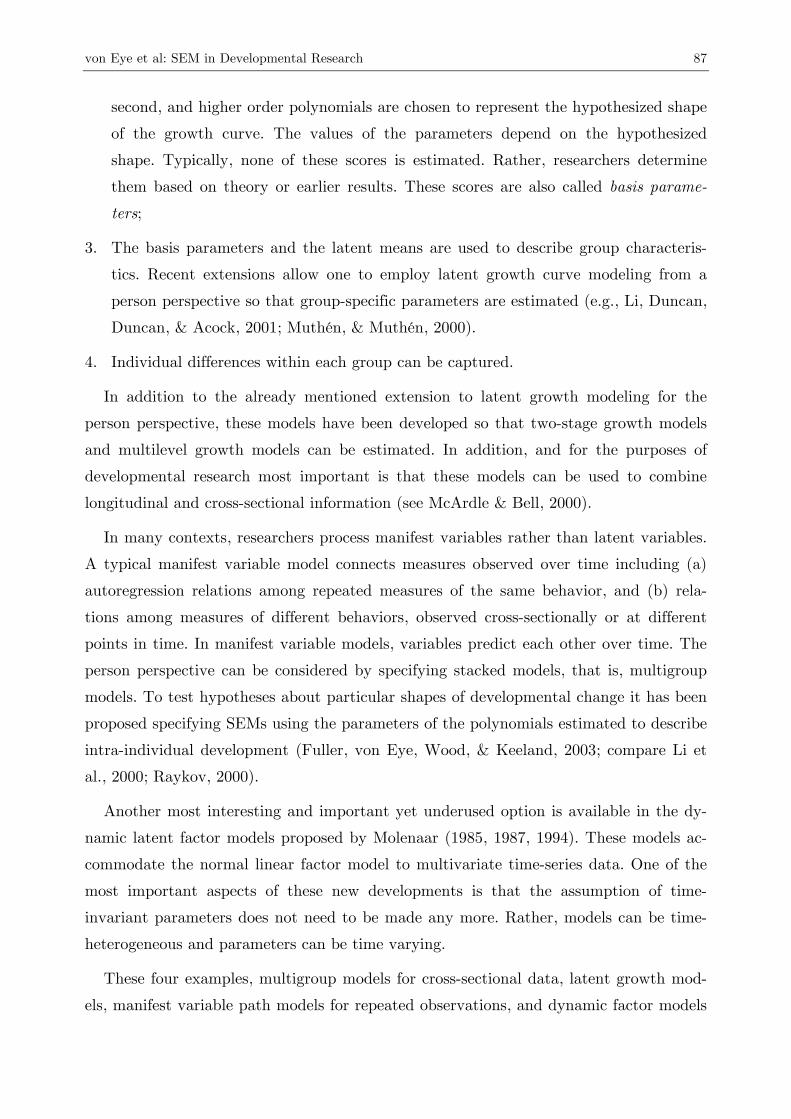
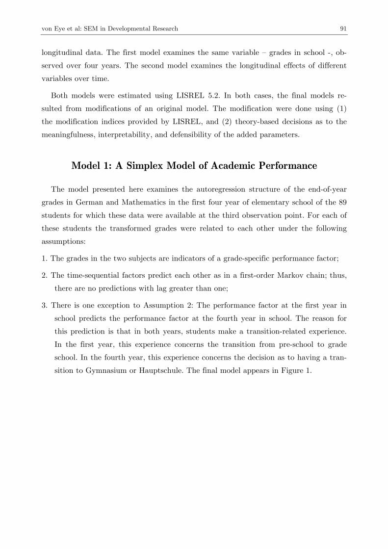
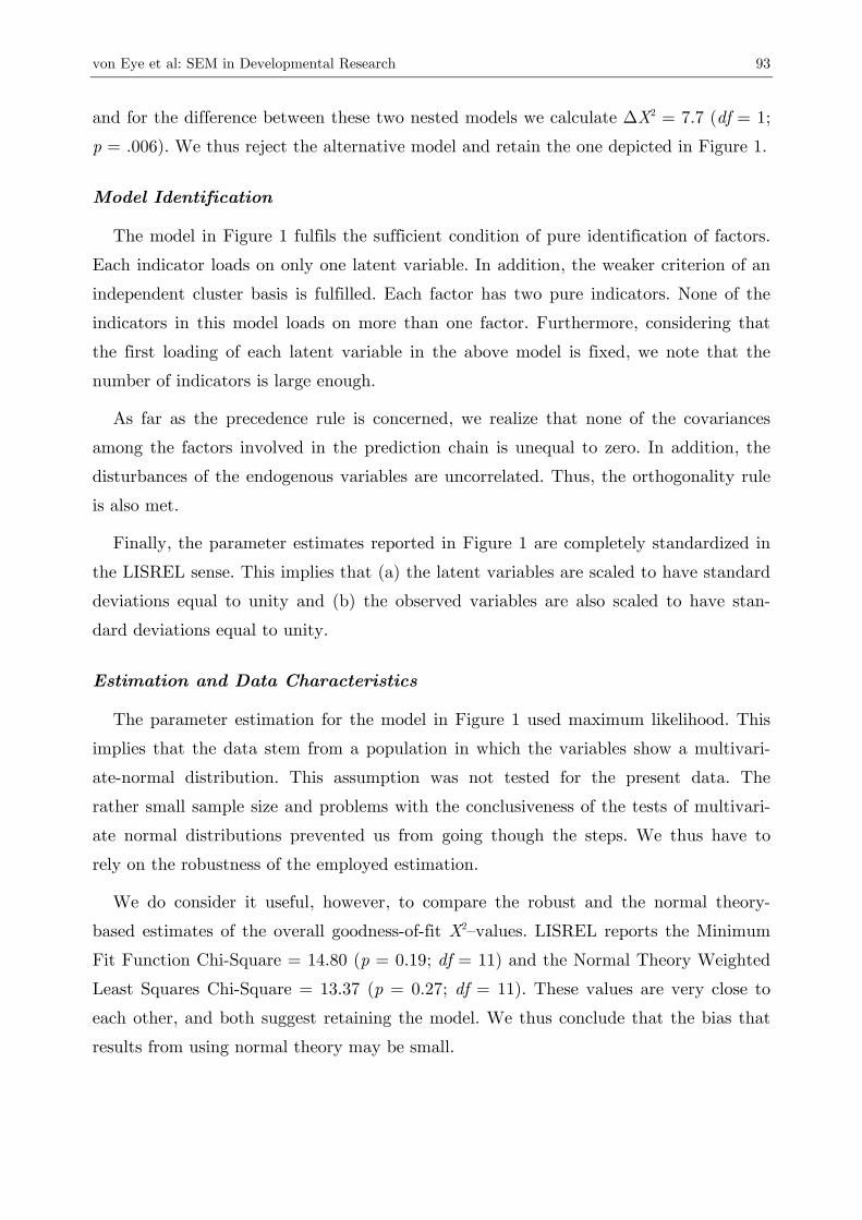
Model 1: A Simplex Model of Academic Performance
The model presented here examines the autoregression structure of the end-of-year
grades in German and Mathematics in the first four year of elementary school of the 89
students for which these data were available at the third observation point. For each of
these students the transformed grades were related to each other under the following
assumptions:
1. The grades in the two subjects are indicators of a grade-specific performance factor;
2. The time-sequential factors predict each other as in a first-order Markov chain; thus,
there are no predictions with lag greater than one;
3. There is one exception to Assumption 2: The performance factor at the first year in
school predicts the performance factor at the fourth year in school. The reason for
this prediction is that in both years, students make a transition-related experience.
In the first year, this experience concerns the transition from pre-school to grade
school. In the fourth year, this experience concerns the decision as to having a tran-
sition to Gymnasium or Hauptschule. The final model appears in Figure 1.
92 MPR-Online 2003, Vol. 8, No. 2
grade11.00
grade20.80
grade30.46
grade40.23
g1 0.27
g2 0.29
g3 0.27
g4 0.42
m1 0.27
m2 0.30
m3 0.08
m4 0.00
Chi-Square=13.37, df=11, P-value=0.27012, RMSEA=0.049
0.85
0.85
0.84
0.84
0.85
0.96
0.76
1.00
0.45
0.73
0.22
0.78
0.26
0.13
0.25
0.20
0.28
Figure 1: Final simplex of academic performance in the first four grades of elementary
school (completely standardized parameters are given; all paths significant)
We now discuss the model with reference to the five characteristics discussed in
“Characteristics of structural models –general”, above.
Model Specification
The issue of model specification concerns the decisions as to which covariances to in-
clude and which covariances not to include. In the present model, it is hypothesized
that grades in school can be sufficiently predicted using information from the previous
year. The first year in school serves as external variable. This does not imply that pre-
dictions that skip one or two years cannot be made. However, the model proposes that
lags greater than one are not needed for a good description of the data. Therefore, none
of the paths for lags greater than one are included in the model. The only exception is
the path from the first to the fourth year, because these years share the transition ele-
ment in common.
Keeping the simplex model pure, that is, omitting the path from Year 1 to Year 4,
yields a model of lesser fit that is significantly worse than the model in Figure 1. More
specifically, for the model without this path, we obtain a X2 = 21.07 (df = 12; p = .049)
von Eye et al: SEM in Developmental Research 93
and for the difference between these two nested models we calculate ∆X2 = 7.7 (df = 1;
p = .006). We thus reject the alternative model and retain the one depicted in Figure 1.
Model Identification
The model in Figure 1 fulfils the sufficient condition of pure identification of factors.
Each indicator loads on only one latent variable. In addition, the weaker criterion of an
independent cluster basis is fulfilled. Each factor has two pure indicators. None of the
indicators in this model loads on more than one factor. Furthermore, considering that
the first loading of each latent variable in the above model is fixed, we note that the
number of indicators is large enough.
As far as the precedence rule is concerned, we realize that none of the covariances
among the factors involved in the prediction chain is unequal to zero. In addition, the
disturbances of the endogenous variables are uncorrelated. Thus, the orthogonality rule
is also met.
Finally, the parameter estimates reported in Figure 1 are completely standardized in
the LISREL sense. This implies that (a) the latent variables are scaled to have standard
deviations equal to unity and (b) the observed variables are also scaled to have stan-
dard deviations equal to unity.
Estimation and Data Characteristics
The parameter estimation for the model in Figure 1 used maximum likelihood. This
implies that the data stem from a population in which the variables show a multivari-
ate-normal distribution. This assumption was not tested for the present data. The
rather small sample size and problems with the conclusiveness of the tests of multivari-
ate normal distributions prevented us from going though the steps. We thus have to
rely on the robustness of the employed estimation.
We do consider it useful, however, to compare the robust and the normal theory-
based estimates of the overall goodness-of-fit X2–values. LISREL reports the Minimum
Fit Function Chi-Square = 14.80 (p = 0.19; df = 11) and the Normal Theory Weighted
Least Squares Chi-Square = 13.37 (p = 0.27; df = 11). These values are very close to
each other, and both suggest retaining the model. We thus conclude that the bias that
results from using normal theory may be small.
94 MPR-Online 2003, Vol. 8, No. 2
Goodness-of-Fit
It is recommended that many goodness-of-fit results be reported, mainly to (a) indi-
cate that discrepant appraisals of model fit are minimal, and (b) to disperse with the
suspicion that authors select the index that presents their final model in the most fa-
vorable light. For the present example, we decided to report the entire goodness-of-fit
information that LISREL makes available to the user. Table 1 contains this informa-
tion.
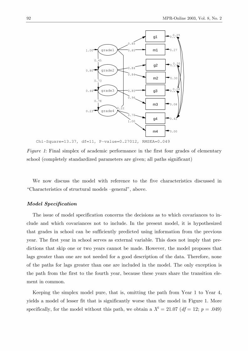
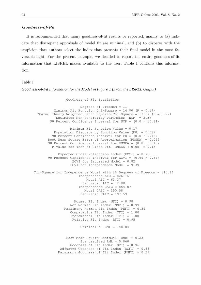
Table 1
Goodness-of-Fit Information for the Model in Figure 1 (From the LISREL Output)
Goodness of Fit Statistics Degrees of Freedom = 11 Minimum Fit Function Chi-Square = 14.80 (P = 0.19) Normal Theory Weighted Least Squares Chi-Square = 13.37 (P = 0.27) Estimated Non-centrality Parameter (NCP) = 2.37 90 Percent Confidence Interval for NCP = (0.0 ; 15.84) Minimum Fit Function Value = 0.17 Population Discrepancy Function Value (F0) = 0.027 90 Percent Confidence Interval for F0 = (0.0 ; 0.18) Root Mean Square Error of Approximation (RMSEA) = 0.049 90 Percent Confidence Interval for RMSEA = (0.0 ; 0.13) P-Value for Test of Close Fit (RMSEA < 0.05) = 0.45 Expected Cross-Validation Index (ECVI) = 0.72 90 Percent Confidence Interval for ECVI = (0.69 ; 0.87) ECVI for Saturated Model = 0.82 ECVI for Independence Model = 9.39 Chi-Square for Independence Model with 28 Degrees of Freedom = 810.16 Independence AIC = 826.16 Model AIC = 63.37 Saturated AIC = 72.00 Independence CAIC = 854.07 Model CAIC = 150.58 Saturated CAIC = 197.59 Normed Fit Index (NFI) = 0.98 Non-Normed Fit Index (NNFI) = 0.99 Parsimony Normed Fit Index (PNFI) = 0.39 Comparative Fit Index (CFI) = 1.00 Incremental Fit Index (IFI) = 1.00 Relative Fit Index (RFI) = 0.95 Critical N (CN) = 148.04 Root Mean Square Residual (RMR) = 0.23 Standardized RMR = 0.060 Goodness of Fit Index (GFI) = 0.96 Adjusted Goodness of Fit Index (AGFI) = 0.88 Parsimony Goodness of Fit Index (PGFI) = 0.29
von Eye et al: SEM in Developmental Research 95
Of the many indices presented in this table, we discuss only a few briefly. First, we
note again that both X2–values suggest that the discrepancies between the model-
created variance-covariance matrix and the empirical variance-covariance matrix are
non-significant. The inspection of the residuals follows below. Second, we find an
RMSEA smaller than the cut-off of 0.05 that is typically used to indicate close fit.
Third, the model AIC scores are smaller than the saturated and the independence AIC
scores. We conclude that the model enabled us to reduce uncertainty. The GFI is a
large 0.96. All other goodness-of-fit indices are very large too. We thus conclude that
none of the goodness-of-fit indicators for the present model would lead us to rejection.
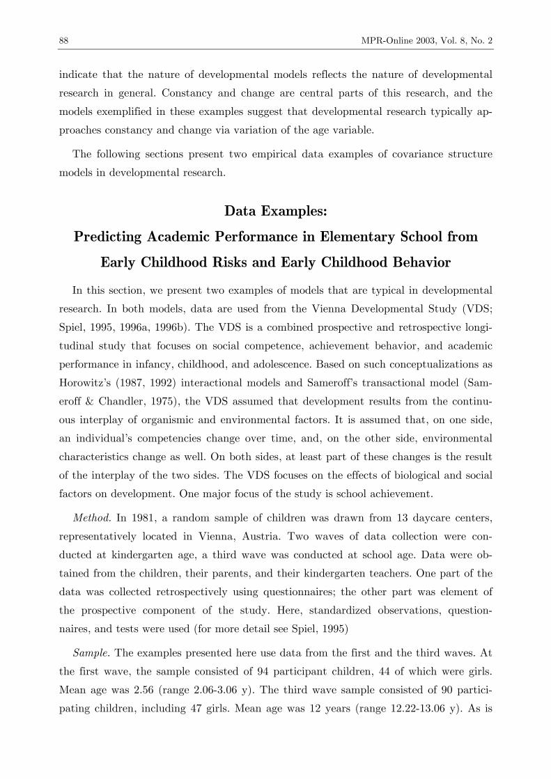
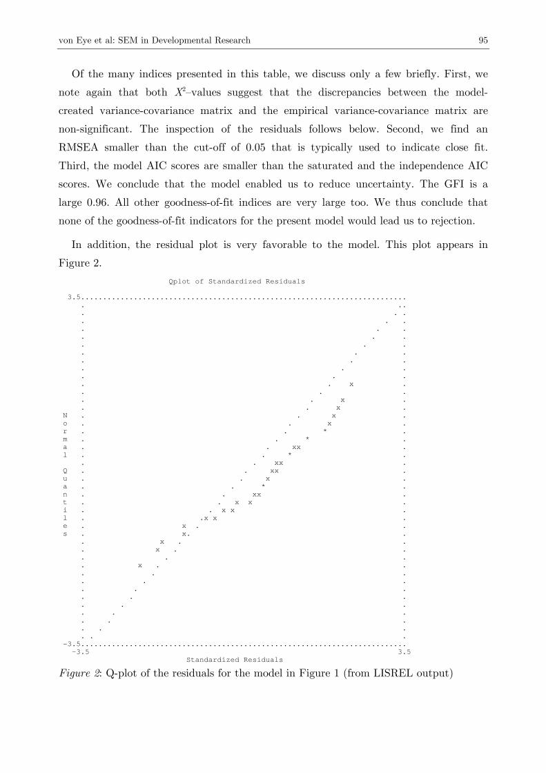
In addition, the residual plot is very favorable to the model. This plot appears in
Figure 2. Qplot of Standardized Residuals 3.5.......................................................................... . .. . . . . . . . . . . . . . . . . . . . . . . . . . . . . . x . . . . . . x . . . x . N . . x . o . . x . r . . * . m . . * . a . . xx . l . . * . . . xx . Q . . xx . u . . x . a . . * . n . . xx . t . . x x . i . . x x . l . .x x . e . x . . s . x. . . x . . . x . . . . . . x . . . . . . . . . . . . . . . . . . . . . . . . . . . . . -3.5.......................................................................... -3.5 3.5 Standardized Residuals
Figure 2: Q-plot of the residuals for the model in Figure 1 (from LISREL output)
96 MPR-Online 2003, Vol. 8, No. 2
Figure 2 shows two of the important characteristics of residual plots that represent a
well-fitting model. First, there is a monotonic increase of residuals that is almost paral-
lel to the optimal line (dotted in the figure). This characteristic suggests that the distri-
bution of the residuals is very near to a normal distribution. Discrepancies are most
likely random. Second, there are no extreme residuals. None of the residual scores comes
even close to the value of 3.5, that is, the extreme ends of the graph. Note that there is
no agreement among methodologists concerning the percentage of extreme residuals that
can be accepted. One group of experts proposes that α-% of the residuals can be ex-
treme. Another group of experts proposes that the existence of extreme residuals sug-
gests that a model shows room for improvement.
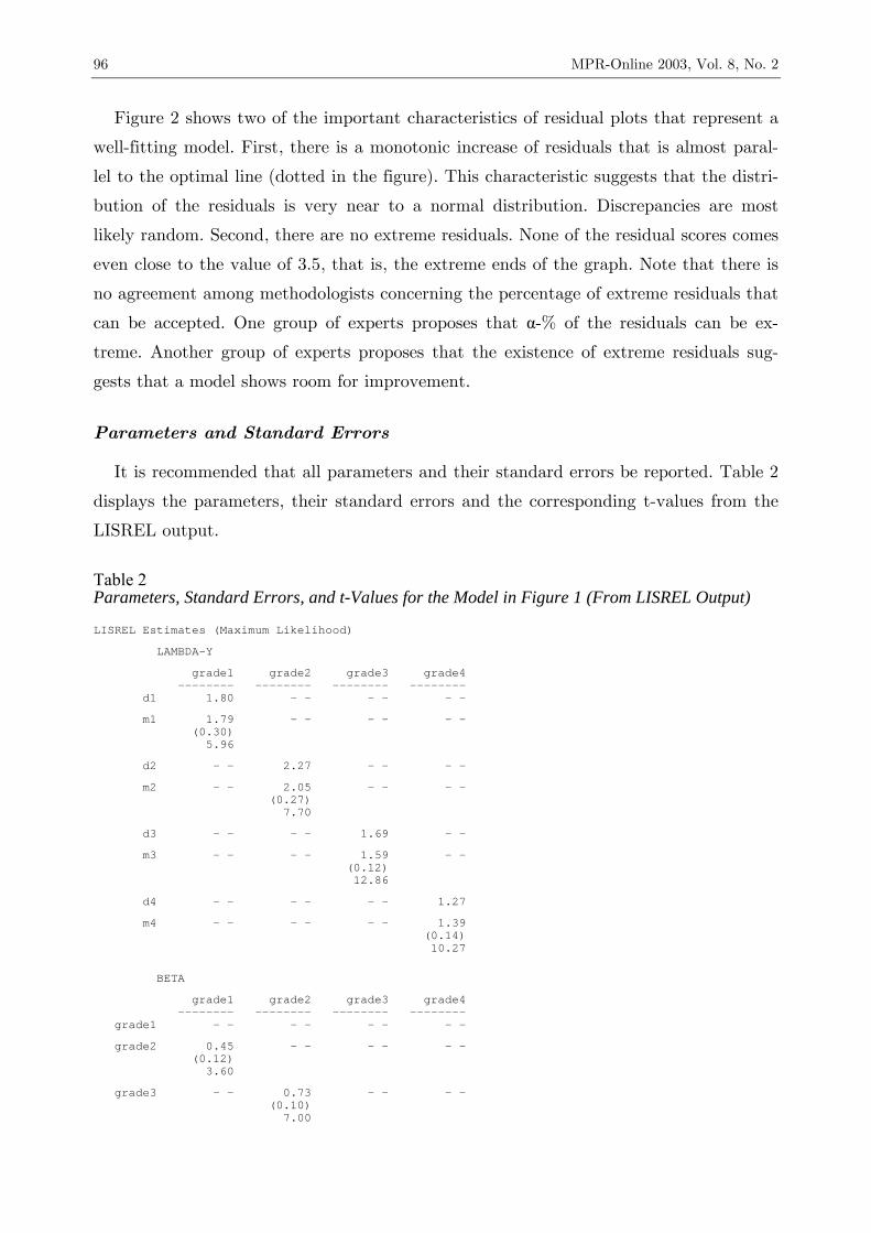
Parameters and Standard Errors
It is recommended that all parameters and their standard errors be reported. Table 2
displays the parameters, their standard errors and the corresponding t-values from the
LISREL output.
Table 2 Parameters, Standard Errors, and t-Values for the Model in Figure 1 (From LISREL Output)
LISREL Estimates (Maximum Likelihood) LAMBDA-Y grade1 grade2 grade3 grade4 -------- -------- -------- -------- d1 1.80 - - - - - - m1 1.79 - - - - - - (0.30) 5.96 d2 - - 2.27 - - - - m2 - - 2.05 - - - - (0.27) 7.70 d3 - - - - 1.69 - - m3 - - - - 1.59 - - (0.12) 12.86 d4 - - - - - - 1.27 m4 - - - - - - 1.39 (0.14) 10.27 BETA grade1 grade2 grade3 grade4 -------- -------- -------- -------- grade1 - - - - - - - - grade2 0.45 - - - - - - (0.12) 3.60 grade3 - - 0.73 - - - - (0.10) 7.00
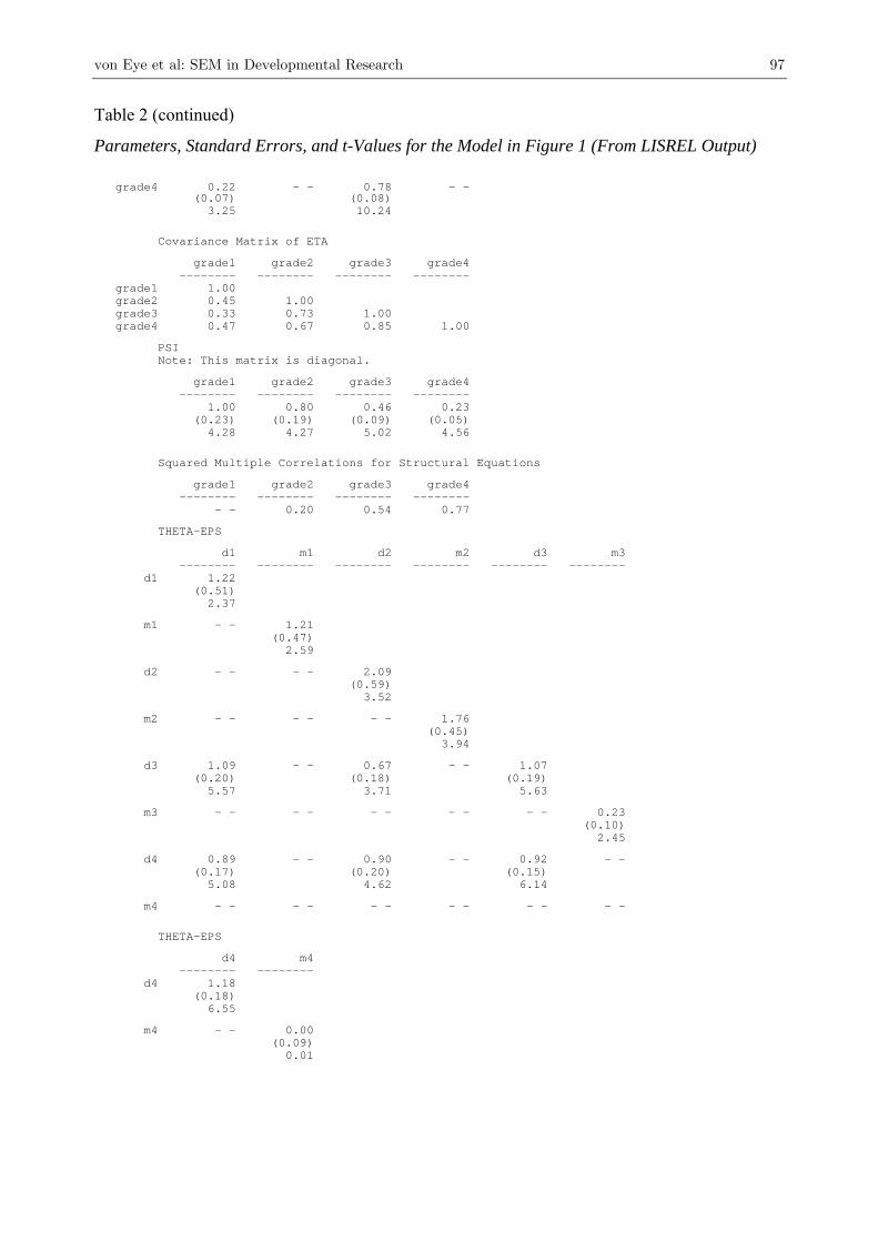
von Eye et al: SEM in Developmental Research 97
Table 2 (continued)
Parameters, Standard Errors, and t-Values for the Model in Figure 1 (From LISREL Output)
grade4 0.22 - - 0.78 - - (0.07) (0.08) 3.25 10.24 Covariance Matrix of ETA grade1 grade2 grade3 grade4 -------- -------- -------- -------- grade1 1.00 grade2 0.45 1.00 grade3 0.33 0.73 1.00 grade4 0.47 0.67 0.85 1.00 PSI Note: This matrix is diagonal. grade1 grade2 grade3 grade4 -------- -------- -------- -------- 1.00 0.80 0.46 0.23 (0.23) (0.19) (0.09) (0.05) 4.28 4.27 5.02 4.56 Squared Multiple Correlations for Structural Equations grade1 grade2 grade3 grade4 -------- -------- -------- -------- - - 0.20 0.54 0.77 THETA-EPS d1 m1 d2 m2 d3 m3 -------- -------- -------- -------- -------- -------- d1 1.22 (0.51) 2.37 m1 - - 1.21 (0.47) 2.59 d2 - - - - 2.09 (0.59) 3.52 m2 - - - - - - 1.76 (0.45) 3.94 d3 1.09 - - 0.67 - - 1.07 (0.20) (0.18) (0.19) 5.57 3.71 5.63 m3 - - - - - - - - - - 0.23 (0.10) 2.45 d4 0.89 - - 0.90 - - 0.92 - - (0.17) (0.20) (0.15) 5.08 4.62 6.14 m4 - - - - - - - - - - - - THETA-EPS d4 m4 -------- -------- d4 1.18 (0.18) 6.55 m4 - - 0.00 (0.09) 0.01
98 MPR-Online 2003, Vol. 8, No. 2
Table 2 shows the estimates for the unstandardized solution. LISREL does not pro-
vide standard errors for the standardized solutions (note, however, that the estimates
for the structural part of the model are the same in the non-standardized and the com-
pletely standardized solutions). We therefore inspect the above solution. None of the
standard errors in this solution is extremely large. This applies to both the parameters
for the measurement and the path models. In addition, the variances of the latent vari-
ables are significantly greater than zero. Their covariances are unequal to zero, too.
However, they are not needed for a satisfactory description of the data at hand.
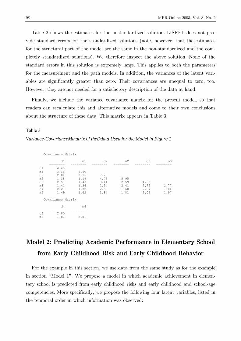
Finally, we include the variance covariance matrix for the present model, so that
readers can recalculate this and alternative models and come to their own conclusions
about the structure of these data. This matrix appears in Table 3.
Table 3
Variance-CovarianceMmatrix of theDdata Used for the Model in Figure 1
Covariance Matrix d1 m1 d2 m2 d3 m3 -------- -------- -------- -------- -------- -------- d1 4.40 m1 3.16 4.40 d2 2.04 2.15 7.28 m2 1.18 1.19 4.75 5.95 d3 2.57 1.43 3.41 2.59 4.03 m3 1.41 1.36 2.54 2.41 2.75 2.77 d4 2.27 1.32 2.59 1.60 2.87 1.84 m4 1.49 1.42 1.84 1.81 2.09 1.97 Covariance Matrix d4 m4 -------- -------- d4 2.85 m4 1.82 2.01
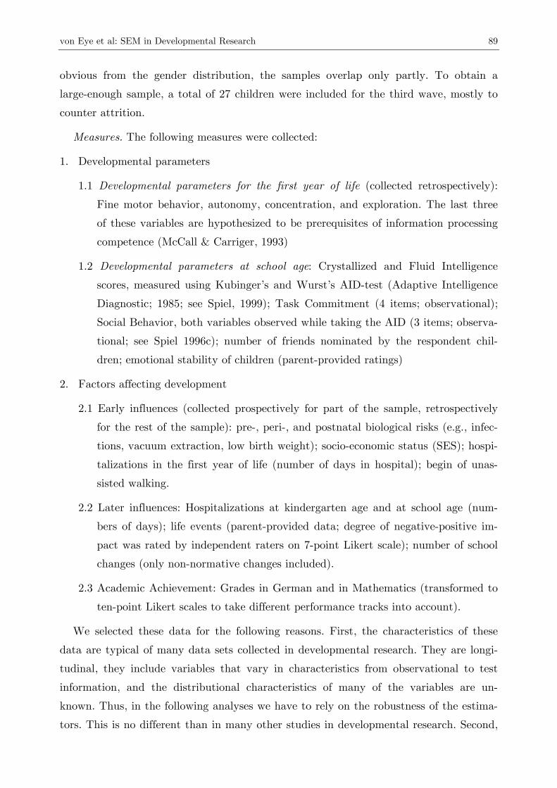
Model 2: Predicting Academic Performance in Elementary School
from Early Childhood Risk and Early Childhood Behavior
For the example in this section, we use data from the same study as for the example
in section “Model 1”. We propose a model in which academic achievement in elemen-
tary school is predicted from early childhood risks and early childhood and school-age
competencies. More specifically, we propose the following four latent variables, listed in
the temporal order in which information was observed:
von Eye et al: SEM in Developmental Research 99
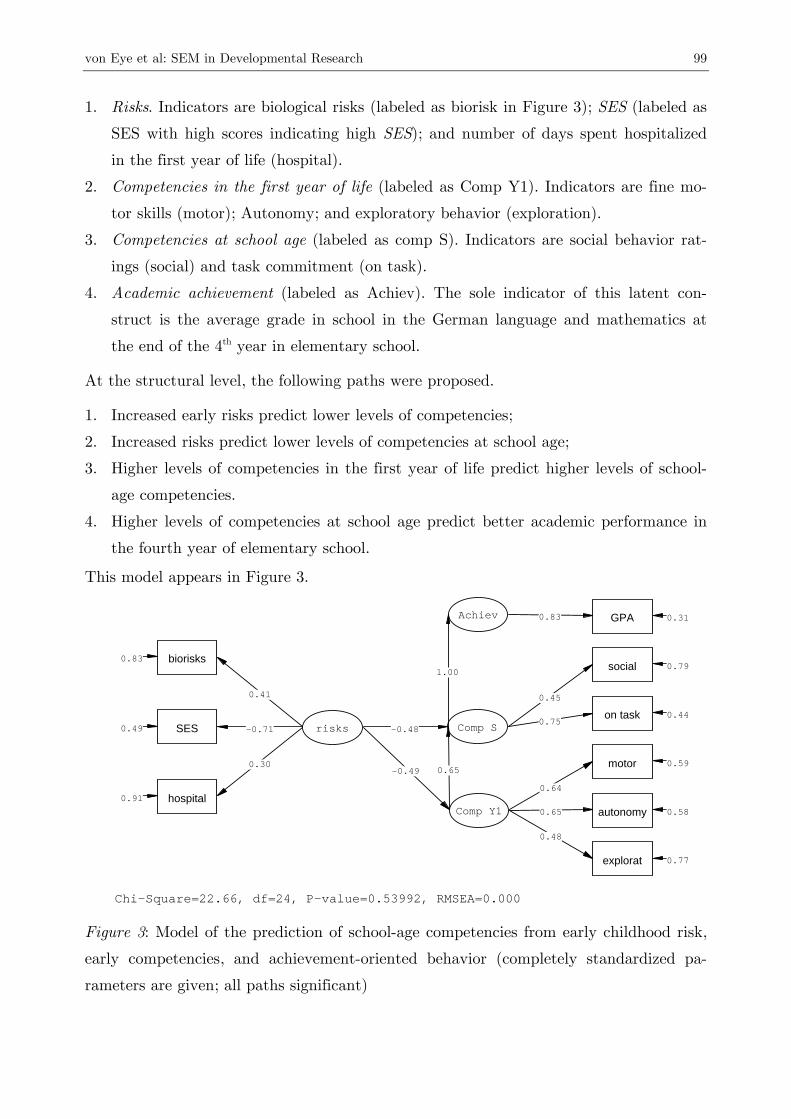
1. Risks. Indicators are biological risks (labeled as biorisk in Figure 3); SES (labeled as
SES with high scores indicating high SES); and number of days spent hospitalized
in the first year of life (hospital).
2. Competencies in the first year of life (labeled as Comp Y1). Indicators are fine mo-
tor skills (motor); Autonomy; and exploratory behavior (exploration).
3. Competencies at school age (labeled as comp S). Indicators are social behavior rat-
ings (social) and task commitment (on task).
4. Academic achievement (labeled as Achiev). The sole indicator of this latent con-
struct is the average grade in school in the German language and mathematics at
the end of the 4th year in elementary school.
At the structural level, the following paths were proposed.
1. Increased early risks predict lower levels of competencies;
2. Increased risks predict lower levels of competencies at school age;
3. Higher levels of competencies in the first year of life predict higher levels of school-
age competencies.
4. Higher levels of competencies at school age predict better academic performance in
the fourth year of elementary school.
This model appears in Figure 3.
biorisks0.83
SES0.49
hospital0.91
risks
Comp Y1
Comp S
Achiev GPA 0.31
social 0.79
on task 0.44
motor 0.59
autonomy 0.58
explorat 0.77
Chi-Square=22.66, df=24, P-value=0.53992, RMSEA=0.000
0.64
0.65
0.48
0.75
0.45
0.83
0.41
-0.71
0.300.65
1.00
-0.49
-0.48
Figure 3: Model of the prediction of school-age competencies from early childhood risk,
early competencies, and achievement-oriented behavior (completely standardized pa-
rameters are given; all paths significant)
100 MPR-Online 2003, Vol. 8, No. 2
In a fashion parallel to the first data example, we now discuss this model with refer-
ence to the five model characteristics presented in the section titled “Characteristics of
structural models –general”.
Model Specification
Obviously, the model in Figure 3 is an indirect effects model. That is, risk is pro-
posed to predict achievement via early competencies and achievement-oriented behav-
ior. To establish an indirect effects model, one needs to run at least the following three
models: (1) the complete model including all indirect and all direct effects; (2) the
model of only indirect effects; and (3) the model of only direct effects. The latter two
models are hierarchically related to the first, but not to each other. One can thus de-
termine whether the latter two model account for significantly less variance than the
complete model. However, there is no way that we are aware of to statistically compare
the two partial effect models. For lack of space, we only report the indirect effect model
here3. This applies accordingly to the direct versus mediated relationship between the
latent variables Comp Y1 and Achiev.
Model Identification
The model in Figure 3 is identified. It fulfills the criteria of pure identification and
independent cluster basis. The number of indicators per latent variable is relatively
small. However, both the path from the achievement factor and the residual of the
achievement indicator were fixed, and so was the variance of the achievement factor.
Thus, the explainable portion of achievement variance resides in the path from the fac-
tor of achievement-oriented behavior to achievement. Fixing these parameters made the
model identified. The discussion of the precedence rule carries over from the first exam-
ple.
Also as in the first example, the parameter estimates presented in Figure 3 are com-
pletely standardized in the LISREL sense.
3 Readers are invited to confirm that the complete model represents only a modest, non-significant im-
provement over the indirect effects model in Figure 3 (X2 = 21.28; df = 23; p = .56; ∆X2 = 1.38; ∆df =
1; n.s.); and that the direct effects-only model represents the data significantly worse than the complete
model (X2 = 28.13; df = 24; p = .25; ∆X2 = 6.85; ∆df = 1; p = .009). We thus retain the indirect effects
model. The command files for the models discussed in the two examples of this article can be obtained
from C. Spiel at [email protected] .
von Eye et al: SEM in Developmental Research 101
Estimation and Data Characteristics
The parameter estimation for the model in Figure 3 used maximum likelihood. As in
the first example, we are not certain that the variables used in the present model stem
from a population in which they follow a multivariate-normal distribution. So again, we
have to rely on the robustness characteristics of the estimators used by LISREL. As in
the first example, we note that the differences between the normal theory-based and the
robust X2–values are minimal. Specifically, we obtain a Minimum Fit Function Chi-
Square = 25.19 (p = .40) and a Normal Theory Weighted Least Squares Chi-Square =
22.66 (p = .54; df = 14 for both). Clearly, both of these values suggest that the model
can be retained.
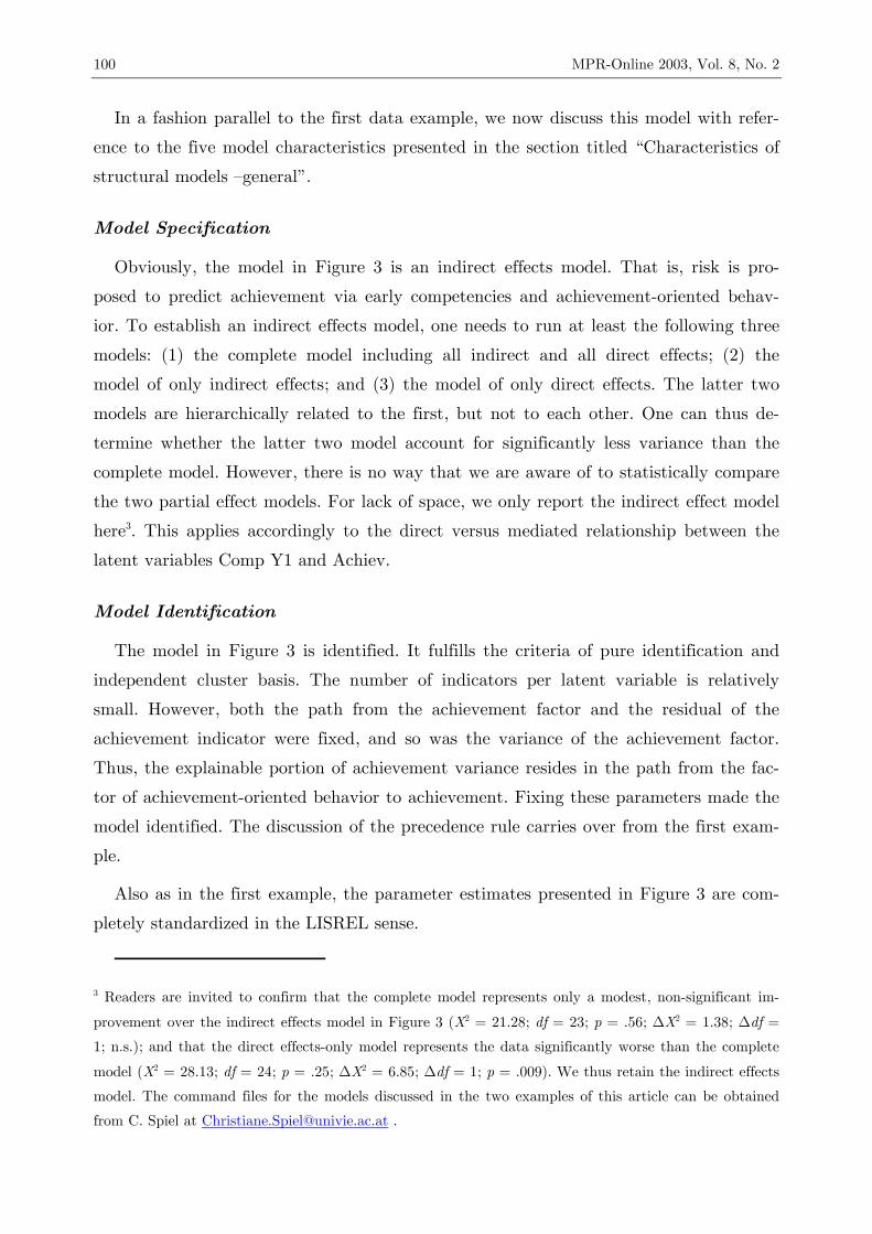
Goodness-of-Fit
Following the recommendation to report a larger number of goodness-of-fit estimates
rather than a small number, we present the entire table of goodness-of-fit statistics pro-
vided by LISREL in Table 4.
As was noted above, both X2–values suggest good model-data fit. The discrepancies
between the model covariance matrix and the empirical covariance matrix are non sig-
nificant. The RMSEA is basically zero, indicating exact fit. The AIC scores indicate
that the model reduced uncertainty in comparison to both the independence and the
saturated models. The goodness-of-fit indices are all close to or at the maximum value
of 1.0. We conclude that none of these indicators suggests that the model misrepresents
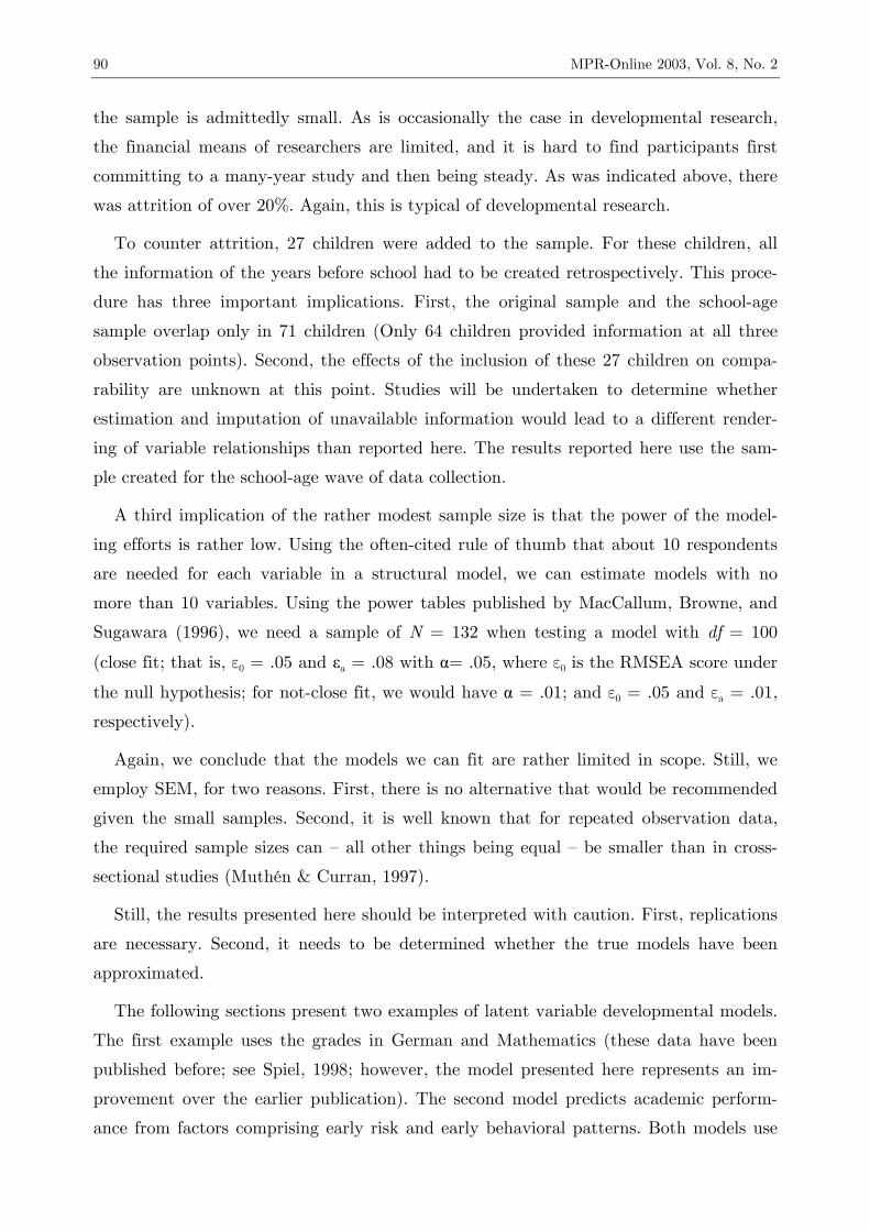
the data. This applies accordingly to the Q-plot of the residuals, which appears in Fig-
ure 4.
102 MPR-Online 2003, Vol. 8, No. 2
Table 4:
Goodness-of-Fit Indicators for the Model in Figure 3 (From the LISREL Output)
Goodness of Fit Statistics Degrees of Freedom = 24 Minimum Fit Function Chi-Square = 25.19 (P = 0.40) Normal Theory Weighted Least Squares Chi-Square = 22.66 (P = 0.54) Estimated Non-centrality Parameter (NCP) = 0.0 90 Percent Confidence Interval for NCP = (0.0 ; 13.81) Minimum Fit Function Value = 0.28 Population Discrepancy Function Value (F0) = 0.0 90 Percent Confidence Interval for F0 = (0.0 ; 0.16) Root Mean Square Error of Approximation (RMSEA) = 0.0 90 Percent Confidence Interval for RMSEA = (0.0 ; 0.080) P-Value for Test of Close Fit (RMSEA < 0.05) = 0.78 Expected Cross-Validation Index (ECVI) = 0.74 90 Percent Confidence Interval for ECVI = (0.74 ; 0.90) ECVI for Saturated Model = 1.01 ECVI for Independence Model = 3.66 Chi-Square for Independence Model with 36 Degrees of Freedom = 308.14 Independence AIC = 326.14 Model AIC = 64.66 Saturated AIC = 90.00 Independence CAIC = 357.64 Model CAIC = 138.16 Saturated CAIC = 247.49 Normed Fit Index (NFI) = 0.92 Non-Normed Fit Index (NNFI) = 0.99 Parsimony Normed Fit Index (PNFI) = 0.61 Comparative Fit Index (CFI) = 1.00 Incremental Fit Index (IFI) = 1.00 Relative Fit Index (RFI) = 0.88 Critical N (CN) = 152.86 Root Mean Square Residual (RMR) = 0.12 Standardized RMR = 0.050 Goodness of Fit Index (GFI) = 0.94 Adjusted Goodness of Fit Index (AGFI) = 0.90 Parsimony Goodness of Fit Index (PGFI) = 0.50
The Q-plot of the residuals of the model in Figure 3 is close to perfect. The residuals
are almost perfectly normally distributed, and they are far from extreme. Each residual
in Figure 4 is indicated by an x, multiple residuals with the same values are indicated
by an asterisk. If the distribution of residuals in a Q-plot is monotonic and close to the
ideal, dotted, line, the residuals can be considered normally distributed. This is the case
in this example.
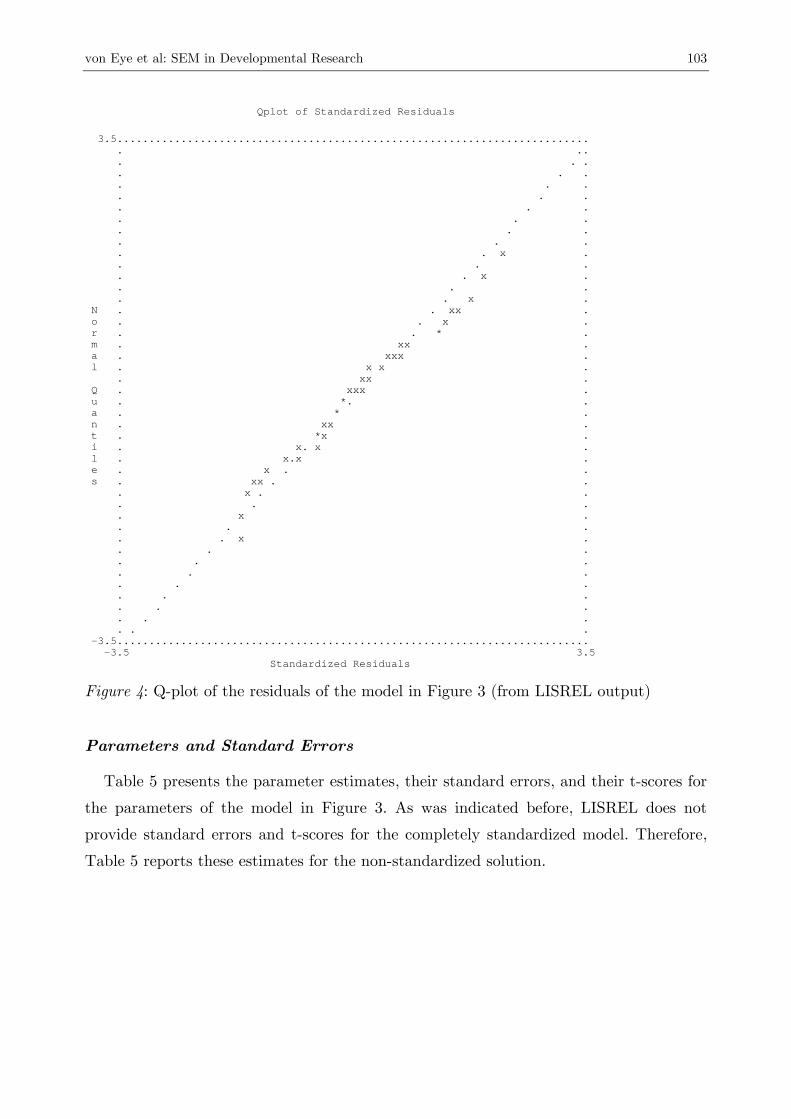
von Eye et al: SEM in Developmental Research 103
Qplot of Standardized Residuals
3.5.......................................................................... . .. . . . . . . . . . . . . . . . . . . . . . . . . . . x . . . . . . x . . . . . . x . N . . xx . o . . x . r . . * . m . xx . a . xxx . l . x x . . xx . Q . xxx . u . *. . a . * . n . xx . t . *x . i . x. x . l . x.x . e . x . . s . xx . . . x . . . . . . x . . . . . . x . . . . . . . . . . . . . . . . . . . . . . . . . -3.5.......................................................................... -3.5 3.5 Standardized Residuals Figure 4: Q-plot of the residuals of the model in Figure 3 (from LISREL output)
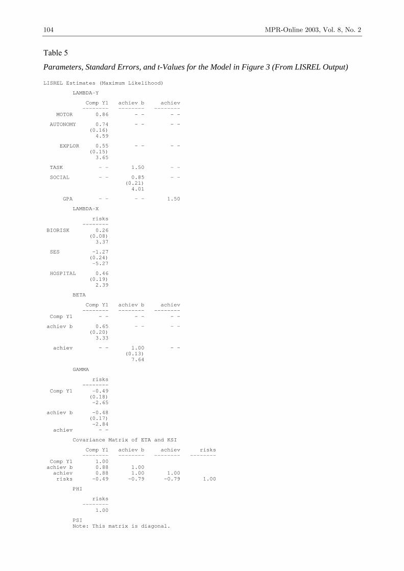
Parameters and Standard Errors
Table 5 presents the parameter estimates, their standard errors, and their t-scores for
the parameters of the model in Figure 3. As was indicated before, LISREL does not
provide standard errors and t-scores for the completely standardized model. Therefore,
Table 5 reports these estimates for the non-standardized solution.
104 MPR-Online 2003, Vol. 8, No. 2
Table 5
Parameters, Standard Errors, and t-Values for the Model in Figure 3 (From LISREL Output)
LISREL Estimates (Maximum Likelihood) LAMBDA-Y Comp Y1 achiev b achiev -------- -------- -------- MOTOR 0.86 - - - - AUTONOMY 0.74 - - - - (0.16) 4.59 EXPLOR 0.55 - - - - (0.15) 3.65 TASK - - 1.50 - - SOCIAL - - 0.85 - - (0.21) 4.01 GPA - - - - 1.50 LAMBDA-X risks -------- BIORISK 0.26 (0.08) 3.37 SES -1.27 (0.24) -5.27 HOSPITAL 0.46 (0.19) 2.39 BETA Comp Y1 achiev b achiev -------- -------- -------- Comp Y1 - - - - - - achiev b 0.65 - - - - (0.20) 3.33 achiev - - 1.00 - - (0.13) 7.64 GAMMA risks -------- Comp Y1 -0.49 (0.18) -2.65 achiev b -0.48 (0.17) -2.84 achiev - - Covariance Matrix of ETA and KSI Comp Y1 achiev b achiev risks -------- -------- -------- -------- Comp Y1 1.00 achiev b 0.88 1.00 achiev 0.88 1.00 1.00 risks -0.49 -0.79 -0.79 1.00 PHI risks -------- 1.00 PSI Note: This matrix is diagonal.
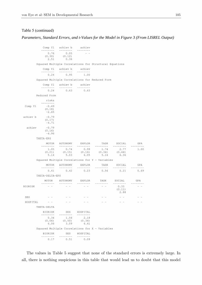
von Eye et al: SEM in Developmental Research 105
Table 5 (continued)
Parameters, Standard Errors, and t-Values for the Model in Figure 3 (From LISREL Output)
Comp Y1 achiev b achiev -------- -------- -------- 0.76 0.05 - - (0.30) (0.12) 2.51 0.36 Squared Multiple Correlations for Structural Equations Comp Y1 achiev b achiev -------- -------- -------- 0.24 0.95 1.00 Squared Multiple Correlations for Reduced Form Comp Y1 achiev b achiev -------- -------- -------- 0.24 0.63 0.63 Reduced Form risks -------- Comp Y1 -0.49 (0.18) -2.65 achiev b -0.79 (0.17) -4.71 achiev -0.79 (0.16) -4.96 THETA-EPS MOTOR AUTONOMY EXPLOR TASK SOCIAL GPA -------- -------- -------- -------- -------- -------- 1.05 0.74 0.99 1.74 2.77 1.00 (0.21) (0.15) (0.16) (0.34) (0.44) 5.14 5.03 6.05 5.16 6.36 Squared Multiple Correlations for Y - Variables MOTOR AUTONOMY EXPLOR TASK SOCIAL GPA -------- -------- -------- -------- -------- -------- 0.41 0.42 0.23 0.56 0.21 0.69 THETA-DELTA-EPS MOTOR AUTONOMY EXPLOR TASK SOCIAL GPA -------- -------- -------- -------- -------- -------- BIORISK - - - - - - - - 0.33 - - (0.11) 2.88 SES - - - - - - - - - - - - HOSPITAL - - - - - - - - - - - - THETA-DELTA BIORISK SES HOSPITAL -------- -------- -------- 0.34 1.56 2.18 (0.06) (0.50) (0.34) 6.06 3.09 6.41 Squared Multiple Correlations for X - Variables BIORISK SES HOSPITAL -------- -------- -------- 0.17 0.51 0.09
The values in Table 5 suggest that none of the standard errors is extremely large. In
all, there is nothing suspicious in this table that would lead us to doubt that this model
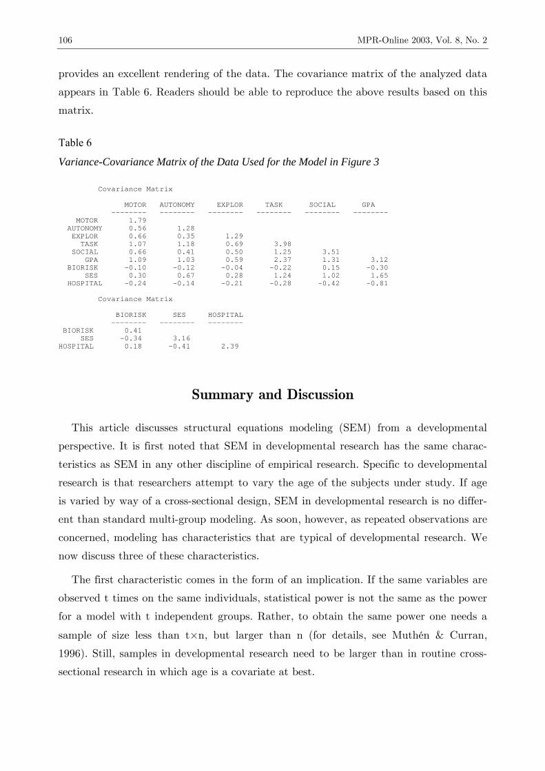
106 MPR-Online 2003, Vol. 8, No. 2
provides an excellent rendering of the data. The covariance matrix of the analyzed data
appears in Table 6. Readers should be able to reproduce the above results based on this
matrix.
Table 6
Variance-Covariance Matrix of the Data Used for the Model in Figure 3
Covariance Matrix MOTOR AUTONOMY EXPLOR TASK SOCIAL GPA -------- -------- -------- -------- -------- -------- MOTOR 1.79 AUTONOMY 0.56 1.28 EXPLOR 0.66 0.35 1.29 TASK 1.07 1.18 0.69 3.98 SOCIAL 0.66 0.41 0.50 1.25 3.51 GPA 1.09 1.03 0.59 2.37 1.31 3.12 BIORISK -0.10 -0.12 -0.04 -0.22 0.15 -0.30 SES 0.30 0.67 0.28 1.24 1.02 1.65 HOSPITAL -0.24 -0.14 -0.21 -0.28 -0.42 -0.81 Covariance Matrix BIORISK SES HOSPITAL -------- -------- -------- BIORISK 0.41 SES -0.34 3.16 HOSPITAL 0.18 -0.41 2.39
Summary and Discussion
This article discusses structural equations modeling (SEM) from a developmental
perspective. It is first noted that SEM in developmental research has the same charac-
teristics as SEM in any other discipline of empirical research. Specific to developmental
research is that researchers attempt to vary the age of the subjects under study. If age
is varied by way of a cross-sectional design, SEM in developmental research is no differ-
ent than standard multi-group modeling. As soon, however, as repeated observations are
concerned, modeling has characteristics that are typical of developmental research. We
now discuss three of these characteristics.
The first characteristic comes in the form of an implication. If the same variables are
observed t times on the same individuals, statistical power is not the same as the power
for a model with t independent groups. Rather, to obtain the same power one needs a
sample of size less than t×n, but larger than n (for details, see Muthén & Curran,
1996). Still, samples in developmental research need to be larger than in routine cross-
sectional research in which age is a covariate at best.
von Eye et al: SEM in Developmental Research 107
The second characteristic is that attrition is typical. In repeated observation studies,
attrition is almost impossible to prevent. The authors know of now long-term study in
which there was no attrition. There are many ways to deal with attrition. First, one can
employ the full information maximum likelihood method. Second, one can estimate and
impute missing information. A third option, which was realized in the examples given in
this article, involves collecting a random sample of data from a parallel cohort that is
then imputed. The characteristics and implications of this procedure are largely un-
known. Future studies will have to determine the degree to which this procedure creates
bias.
The third characteristic concerns the model specifications used to represent the data.
Growth curve models and path models of repeated observations differ from models of
curvilinear relations in cross-sectional studies. For example, growth curve models repre-
sent dependent data, because the same individuals are repeatedly observed. Curvilinear
models of functions such as the one that describes the Weber-Fechner law can be speci-
fied using cross-sectional data. McArdle’s convergence models reside between these ex-
tremes. The main difference is that covariances between time-adjacent observations or,
in more general terms, covariances between observations from different scale points of
some predictor variable can be estimated only if the same individuals are involved. In
cross-sectional designs, these covariances are not defined. The examples presented in
this article used longitudinal data and the models included parameters for the cross-
time covariances.
References
Arbuckle, J. L. (1997). Amos users’ guide. Version 3.6. Chicago: Small Waters.
Baltes, P. B., Reese, H. W., & Nesselroade, J. R. (1977). Life-span developmental psy-
chology: Introduction to research methods. Monterey, CA: Brooks/Cole.
Bayley, N. (1956). Individual patterns of development. Child Development, 27, 45-74.
Bentler, P. M. (1995). EQS structural equation program manual. Encino, CA: Multiva-
riate Software.
Bentler, P. M. (2000). Rites, wrong, and gold in model testing. Structural Equation
Modeling, 7, 82-91.
Bentler, P. M., & Weeks, D. G. (1980). Linear structural equations with latent vari-
ables. Psychometrika, 45, 289-308.
108 MPR-Online 2003, Vol. 8, No. 2
Boomsma, A. (2000). Reporting analyses of covariance structures. Structural Equation
Modeling, 7, 461-483.
Browne, M. W. (1984). Asymptotically distribution free methods for the analysis of co-
variance structures. British Journal of Mathematical and Statistical Psychology, 37,
62-83.
Fuller, B. E., von Eye, A., Wood, P. K., & Keeland, B. (2003). Modeling manifest vari-
ables in longitudinal designs - a two-stage approach. In B. H. Pugesek, A. Tomer, &
A. von Eye (Eds.), Structural equations modeling: applications in ecological and evo-
lutionary biology research (pp. 312-351). Cambridge: Cambridge University Press.
Ghisletta, P., & McArdle, J. J. (2001). Latent growth curve analysis of the development
of height. Structural Equation Modeling, 8, 531-555.
Hayduk, L. A., & Glaser, D. N. (2000). Jiving the four-step waltzing around factor
analysis, and other serious fun. Structural Equation Modeling, 7, 1-35.
Hershberger, S. L. (1994). The specification of equivalent models before the collection of
data. In A. von Eye, & C. C. Clogg (Eds.), Latent variables analysis: Applications to
developmental research (pp. 68-108). Thousand Oaks, CA: Sage.
Horowitz, F. D. (1987). Exploring developmental theories: Toward a structural behavior
model of development. Hillsdale, NJ: Erlbaum.
Horowitz, F. D. (1992). The risk-environment interaction and developmental outcome:
A theoretical perspective. In Ch. W. Greenbaum & J. G. Auerbach (Eds.), Longitu-
dinal studies of children at psychological risk: Cross-national perspectives (pp. 29-
39). Norwood, NJ: Ablex.
Hussy, W., & von Eye, A. (1988). On cognitive operators in information processing and
their effects on memory in different age groups. In F. E. Weinert & M. Perlmutter
(Eds.), Memory development: Universal changes and individual differences (pp. 275-
291). Hillsdale, NJ: Lawrence Erlbaum.
Jöreskog, K. G. (1966). Testing a simple structure hypothesis in factor analysis. Psy-
chometrika, 31, 165-178.
Jöreskog, K. G. (1977). Structural equation models in the social sciences: specification,
estimation and testing. In P. R. Krishnaiah (Ed.), Applications of statistics (pp.
265-287). Amsterdam: North Holland.
Jöreskog, K. G., & Sörbom, D. (1993). LISREL 7 – A guide to the program and appli-
cations. Chicago: SPSS Publications.
Kubinger, K. D., & Wurst, E. (1985). Adaptives Intelligenzdiagnostikum [Adaptive intel-
ligence diagnostics]. Weinheim, Germany: Beltz.
von Eye et al: SEM in Developmental Research 109
Li, F., Duncan, T.E., Duncan, S. C., & Acock, A. (2001). Latent growth modeling of
longitudinal data: A finite mixture modeling approach. Structural Equation Model-
ing, 8, 493-530.
Little, T. D., Schnabel, K. U., & Baumert, J. (Eds.)(2000). Modeling longitudinal and
multilevel data. Practical issues, applied approaches, and specific examples. Mahwah,
NJ: Erlbaum.
MacCallum, R. C., Browne, M. W., & Sugawara, H. M. (1996). Power analysis and de-
termination of sample size for covariance structure modeling. Psychological Methods,
1, 130-149.
McArdle, J. J., & Bell, R. Q. (2000). An introduction to latent growth models for de-
velopmental data analysis. In T. D. Little, K. U. Schnabel, & J. Baumert,
(Eds.)(2000). Modeling longitudinal and multilevel data. Practical issues, applied ap-
proaches, and specific examples (pp. 69-107). Mahwah, NJ: Erlbaum.
McArdle, J. J., & Hamagami, F. (1991). Modeling incomplete longitudinal and cross-
sectional data using latent growth structural models. Experimantal Aging Research,
18, 145-166.
McDonald, R.P. (1997). Haldane’s lungs: A case study in path analysis. Multivariate
Behavioral Research, 32, 1-38.
McDonald, R. P. (in press). What can we learn from the path equations? Psychometrika
McDonald, R. P., & Ho, M.-H. R. (2002). Principles and practice in reporting structural
equation analyses. Psychological Methods, 7, 64-82.
Meredith, W., & Tisak, J. (1990). Latent curve analysis. Psychometrika, 55, 107-122.
Micceri, T. (1989). The unicorn, the normal curve and other improbable creatures. Psy-
chological Bulletin, 105, 156-165.
Molenaar, P. C. M. (1985). A dynamic factor model for the analysis of multivariate
time series. A dynamic factor model for the analysis of multivariate time series.
Psychometrika, 50, 181-202.
Molenaar, P. C. M. (1987). Dynamic factor analysis in the frequency domain: Causal
modeling of multivariate psychophysiological time series. Multivariate Behavioral
Research, 22, 329-353.
Molenaar, P. C. M. (1994). Dynamic latent variable models in developmental psychol-
ogy. In A. von Eye, & C. C. Clogg (Eds.), Latent variables analysis: Applications for
developmental research (pp. 155-180). Thousand Oaks, CA: Sage.
Muthén, B. (1984). A general structural equation model with dichotomous, ordered
categorical and continuous latent variable indicators. Psychometrika, 49, 115-132.
110 MPR-Online 2003, Vol. 8, No. 2
Muthén, B., & Curran, P. (1997). General longitudinal modeling of individual differ-
ences in experimental designs: a latent variable framework for analysis and power
estimation. Psychological Methods, 2, 371-402.
Muthén, B., & Muthén, L. (2000). Integrating person-centered and variable-centered
analyses: Growth mixture modeling with latent trajectory classes. Alcoholism: Clini-
cal and Experimental Research, 24, 882-891.
Neale, M. C. (1997). Mx: Statistical modeling. Box 980126 MCV, Richmond, VA 23298,
4th ed. Computer program.
Pearl, J. (2000). Causality: Models, reasoning, and inference. Cambridge, United King-
dom: Cambridge University Press.
Rao, C. R. (1958). Some statistical methods for comparison of growth curves. Biomet-
rics, 13, 1 – 17.
Raykov, T. (2000). Modeling simultaneously individual and group patterns of ability
growth or decline. In T. D. Little, K. U. Schnabel, & J. Baumert (Eds.). Modeling
longitudinal and multilevel data. Practical issues, applied approaches, and specific
examples (pp. 127-146). Mahwah, NJ: Erlbaum.
Raykov, T., & Penev, S. (1999). On structural equation model equivalence. Multivariate
Behavioral Research, 34, 199-244.
Sameroff, A. J. & Chandler, M. J. (1975). Reproductive risk and the continuum of care-
taking casualty. In F. D. Horowitz, M. Hetherington, S. Scarr-Salapatek & G. Siegel
(Eds.), Review of child development research (Vol.4, pp. 187-244). Chicago: Univer-
sity of Chicago Press. Satorra, A., & Bentler, P. P. (1994). Corrections to standard errors in covariance struc-
ture analysis. In A. von Eye, & C. C. Clogg (Eds.), Latent variable analysis: Appli-
cations to developmental research (pp. 399-419). Thousand Oaks, CA: Sage.
Spiel, C. (1995, unpublished). Erfolg in der Schule. Ein dynamisches Modell der Effekte
biologischer und sozialer Faktoren für die Entwicklung [Success in school. A dynamic
model of the effects of biological and social factors on development]. Universität
Wien.
Spiel, C. (1996a). Long-term effects of minor biological and psychosocial risks on cogni-
tive competence, school achievement, and personality traits. In S. Harel & J. P.
Shonkoff (Eds.), Early childhood intervention and family support programs: Accom-
plishments and challenges (pp. 223-242). Jerusalem: JDC - Brookdale Institute of
Gerontology and Human Development.
von Eye et al: SEM in Developmental Research 111
Spiel, C. (1996b). Effekte leichter biologischer und leichter sozialer Risiken auf Leis-
tungsverhalten im Schulalter –Ergebnisse der Wiener Entwicklungsstudie (WES)
[Effects of moderate biological and social risks on performance behavior during
school age –results of the Vienna Development Research]. In C. Spiel, U. Kastner-
Koller, & P. Deimann (Eds.), Motivation und Lernen aus der Perspektive lebenslan-
ger Entwicklung (pp. 41-59). Münster, Germany: Waxmann.
Spiel. C. (1996c). Verhalten bei Leistungsanforderung: Aufgabenzuwendung, Aktivitäts-
niveau und Sozialverhalten –Eine Revision des Beiblatts "Arbeitshaltungen" des AID
[Behavior during performance requirement: Task attention, level of activity, and so-
cial behavior –a revision of the supplement “attitudes toward work” of the AID].
Zeitschrift für Differentielle und Diagnostische Psychologie, 17, 48-55.
Spiel, C. (1998). Four methodological approaches for the study of stability and change
in development. Methods of Psychological Research online 3. Retrieved August,
2003, from http://www.mpr-online.de .
Spiel, C. (1999). A strategy for data reanalyses in longitudinal studies. In R. K. Sil-
bereisen & A. von Eye (Eds.), Growing up in times of social change (pp. 245-260).
Berlin, Germany: De Gruyter.
Steiger, J. H. (2000). Point estimation, hypothesis testing, and interval estimation using
the RMSEA: Some comments and a reply to Hayduk and Glaser. Structural Equa-
tion Modeling, 7, 149-162.
Thurstone, L. L. (1931). The theory of multiple factors. Ann Arbor, MI: Edwards
Brothers.
Tisak, J., & Meredith, W. (1990). Longitudinal factor analysis. In A. von Eye (Ed.),
Statistical methods in longitudinal research. Vol. 1: Principles and structuring
change (pp. 125-149). Boston: Academic Press.
Tomer, A. (2003). A short history of structural equation models. In B.H. Pugesek, A.
Tomer, & A. von Eye (Eds.), Structural equation modeling: Applications in ecology
and evolutionary biology (pp. 85-124). Cambridge, United Kingdom: Cambridge
University Press
Tomer, A., & Pugesek, B. H. (2003). Guidelines for publication of structural equation
models. In B.H. Pugesek, A. Tomer, & A. von Eye (Eds.), Structural equation mod-
eling: Applications in ecology and evolutionary biology (pp. 125-140). Cambridge,
United Kingdom: Cambridge University Press
Tucker, L.R. (1958). Determination of parameters of a functional relation by factor
analysis. Psychometrika, 23, 19-23.
112 MPR-Online 2003, Vol. 8, No. 2
von Eye, A. (2002). Configural Frequency Analysis - Methods, Models, and Applications.
Mahwah, NJ: Lawrence Erlbaum.
von Eye, A., & Bergman, L. R. (in press). Research strategies in developmental psycho-
pathology: Dimensional identity and the person-oriented approach. Development and
Psychopathology.
von Eye, A., & Fuller, B. E. (2003). A comparison of the SEM software packages
LISREL, EQS, and Amos. In B. Pugesek, A. Tomer, & A. von Eye (Eds.), Struc-
tural equations modeling: applications in ecological and evolutionary biology research
(pp. 355-391). Cambridge: Cambridge University Press.
von Eye, A., & Spiel, C. (1995). Human developmental research: Methodology. In F. E.
Weinert (Ed.), International Encyclopedia of Education, Vol. V, Section Human De-
velopment (pp. 2673-2677). Oxford, United Kingdom: Pergamon.
Wright, S. (1918). On the nature of size factors. Genetics, 3, 367-374.


![[MS-OFFDI]: Microsoft Office File Format Documentation … · 2017-09-19 · Microsoft Word 97 Microsoft Word 2000 Microsoft Word 2002 Microsoft Office Word 2003 Microsoft Office](https://img.pdfslide.net/doc/110x75/5edde022ad6a402d66691993/ms-offdi-microsoft-office-file-format-documentation-2017-09-19-microsoft-word.jpg)


![[MS-OFFDI]: Microsoft Office File Format Documentation ...MS... · Microsoft PowerPoint 2010 Microsoft PowerPoint 2013 Microsoft Word 97 Microsoft Word 2000 Microsoft Word 2002 Microsoft](https://img.pdfslide.net/doc/110x75/5ea61160271e716b297d501f/ms-offdi-microsoft-office-file-format-documentation-ms-microsoft-powerpoint.jpg)