1

Microwave radiometer measurements at Chilbolton

Liquid water path algorithm development and accuracy

by

P.M. Simpson, E.C. Brand, C.L. Wrench

July 2002

Radio Communications Research Unit CLRC-Rutherford Appleton Laboratory

Chilton, DIDCOT, Oxon. OX11 0QX, UK.

RutherfordAppletonLaboratory

FP5 - CLOUDNET Project Report

2

CONTENTS

1. INTRODUCTION.

1.1 Liquid water clouds 1.2 Microwave emission from the atmosphere 1.3 Liquid water path retrieval 2. MICROWAVE RADIOMETERS.

2.1 Radiometer description. 2.2 Radiometer calibration.

3. LIQUID WATER PATH RETRIEVAL ALGORITHM. 3.1 Relationship between radiometer output and atmospheric water. 3.2 Algorithm development Training Set. 3.3 Radiative transfer model. 3.4 Analysis of radiosonde data. 3.5 Transfer Function retrievals. 3.6 Deriving atmospheric properties from radiosonde data.

3.6.1 Water vapour pressure. 3.6.2 Air density. 3.6.3 Water vapour mixing ratio. 3.6.4 Water vapour density. 3.6.5 Relative Humidity. 3.6.6 Cloud liquid water content.

4. RESULTS. 4.1 Calibration of RCRU microwave radiometers, and sources of error.

4.1.1 Offset caused by dielectric lens in radiometer horn antenna. 4.2 Validation of measurements.

4.2.1 The scale height of water vapour in Southern England. 4.2.2 A comparison between measured and predicted brightness

temperature. 4.3 Brightness Temperature estimates from radiosonde measurements. 4.4 Comparison of water vapour path estimates from radiometer

observations, GPS receivers, and radiosonde measurements. 4.5 Clouds and rain. 4.6 Error estimates 4.6.1 Brightness temperature 4.6.2 Water vapour path and liquid water path 5. CONCLUSION.

REFERENCES.

3

1 INTRODUCTION This report concerns the accuracy with which cloud liquid water that is present along a vertical path through the atmosphere can be estimated by making brightness temperature measurements with multi-frequency microwave radiometers.

1.1 Liquid water clouds Water is one of the most variable of the atmosphere’s constituents. It occurs in all three states of matter (solid ice crystals, liquid water droplets, and vapour); its abundance and spatial distribution vary continuously. Liquid water content (LWC) of cloud is usually defined as the mass of liquid water per unit volume of air (expressed in g/m3). By integrating the LWC along a path through the atmosphere, the value of liquid water path (LWP) can be established.

In the UK, the majority of clouds form as layers of stratus and stratocumulus; typically they are less than 2 km thick, have a base at an altitude of about 1 km. and have densities of ~0.3 g/m3. Where deep convection occurs to create the tallest cumulus clouds, LWC can reach much higher values; however, for the non-precipitating clouds that are the subject of this study, the LWC at cloud base is normally about 0.1 g/m3, typically rising to 0.5 g/m3 just below cloud top.

1.2 Microwave emission from the atmosphere

In the microwave region there is a broad spectrum of radiation emitted by atmospheric water; this is significantly enhanced at 22, and 183 GHz by the rotational absorption bands of the polar water vapour molecules. The intensity of microwave radiation emitted at specific frequencies depends on the amount of water occurring in each phase. One way of determining levels of water vapour and liquid water in the atmosphere is to measure emissions with very sensitive microwave radiometers.

It has been shown that a zenith-pointing ground-based microwave receiver measuring sky brightness temperature in the region of 22 GHz is three times more sensitive to the amount of water vapour than the amount of liquid water. However, in the region of 30 GHz the sky brightness temperature is twice as sensitive to liquid water as to water vapour. (Sensitivity to ice is negligible at both frequencies.)

Given this variation of sensitivity it is possible to estimate the amounts of atmospheric water vapour and cloud liquid water by combining measurements of the sky brightness temperature at ~22 GHz and ~30 GHz.

1.3 Liquid water path retrieval

To establish statistical distributions of cloud liquid water the RCRU has designed and built radiometers operating at frequencies of 22.2 GHz, 28.8 GHz and 37.5 GHz. These have been installed at the Chilbolton observatory in Hampshire, UK. Current estimates of retrieval accuracy based on two frequencies are +/-0.1 cm for precipitable water, and +/-28 g/m2 for liquid water path. This improves to +/-24g/m2 when using all three frequencies. It is hoped that one more

4

radiometers at 78 GHz, will be added in the near future to improve the sensitivity to low levels of liquid water.

This report contains a description of measurements made at Chilbolton, the development of an algorithm used to estimate the atmospheric water vapour and cloud liquid water content from measurements of sky brightness temperature, and initial results that illustrate the effectiveness of the retrieval technique.

5

2 MICROWAVE RADIOMETERS.

Microwave radiometers measure incoherent radiant electromagnetic energy. From the ground, zenith pointing radiometers measure energy radiated (emitted) by atmospheric gases, and liquid water in the form of cloud and rain; that energy is dependent on the measurement frequency, and is proportional to the amount of material present in the atmosphere. Radiometer measurements at selected frequencies are used to make estimates of integrated water vapour path and liquid water path.

2.1 Radiometer description.

The RCRU radiometers have been designed to detect microwaves in two bands. For example, the 22.235 GHz radiometer detects signals in the bands 21.685-22.085 GHZ and 22.385 – 22.785 GHz. These two bands lie on either side of a water vapour absorption line. The 28.8 GHz radiometer bands are between 28.25 – 28.65 and 28.95 – 29.35 GHz.

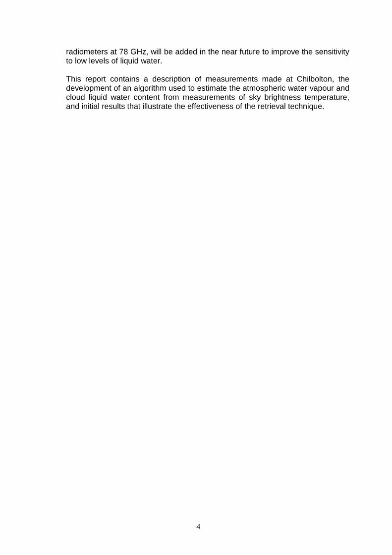
The receiving beamwidths of the three RCRU radiometers are ~2.5o, so that at typical cloud heights from 1 km to 5 km the radiometers are viewing cross-sectional areas of 40x40 m and 220x220 m respectively. This compares with cumulus cloud sizes that range from a few tens of metres to a few hundred metres across. Deep convective clouds can be larger still. The RCRU radiometers are mounted horizontally on a bench inside a temperature controlled cabin at the Chilbolton Observatory. They look through tailored openings in the cabin wall, and view the sky at zenith via an external metal reflector plate mounted at a 45o angle.

RCRU microwave radiometers

6

2.2 Radiometer Calibration.

One method of calibrating radiometers is to measure their output voltages when viewing black-body targets of known temperatures, normally hot (ambient) and cold (liquid nitrogen). This relates the microwave emission from the targets directly to their temperatures. The method relies on there being a linear variation of detector output voltage with target temperature. (This is analogous to calibrating a common mercury bulb thermometer by immersing the bulb in an ice-water mixture and in boiling water). The intensity of microwave radiation from the atmosphere is then expressed as the equivalent Brightness Temperature (BT or Tb, measured in degrees Kelvin), the temperature of a Black Body that would emit the same microwave radiation as the atmosphere. The cold load used to calibrate the RCRU radiometers is provided by a dewar containing a black body target that is immersed in liquid Nitrogen giving a temperature of 77 K. The hot load is a black body (Eccosorb) target at room temperature (approximately 293 K). The receiving horn through which each radiometer receives the atmospheric radiation has a dielectric lens that is designed to ensure a plane wavefront enters the waveguide. The material of the lens introduces some loss so that additional noise is introduced between the radiometer receiver and the sky; it is not incorporated in the calibration procedure, so there are offsets to the brightness temperatures at both frequencies. These offsets are estimated by comparing radiometer brightness temperature measurements with values calculated from an analysis of simultaneous radiosonde ascent measurements.

7

2.3 Radiometer Characteristics

Table 2.1 contains details of the RCRU radiometers that are currently operating at Chilbolton, and one that it is planned to operate in the near future (italics). The addition of a radiometer at 78 GHz would increase sensitivity to thin cloud cover.

Table 2-1 Specification of RCRU Microwave Radiometers (RMR)

FREQUENCY 2 2 . 2 G H z 2 8 . 8 G H z 3 7 . 5 G H z 7 8 G H z 3 d B b e a m w i d t h 2 . 3 d e g . 2 . 3 d e g . 2 d e g . ~ 2 d e g I n t e g r a t i o n t i m e 1 0 s e c o n d s 1 0 s e c o n d s 1 0 s e c o n d s 1 0 s e c o n d s M e a s u r e m e n t 0 . 5 K 0 . 5 K 0 . 5 K 1 K r e s o l u t i o n B a n d w i d t h + / -4 0 0 M H z + / -4 0 0 M H z + / -4 0 0 M H z + / - 4 0 0 M H z

8

3 LIQUID WATER PATH RETRIEVAL ALGORITHM.

3.1 Relationship between radiometer output and atmospheric water. Radiometers are passive instruments that sense downwelling radiation within a conical volume of the sky. Individually, the zenith pointing Chilbolton radiometers measure at frequencies that are sensitive to both the total amount of water vapour and liquid water in the atmosphere, they cannot partition the radiation. Water Vapour Path (WVP), is the depth of water that could be condensed out of an atmospheric column of uniform cross-sectional area (also commonly referred to as Integrated Precipitable Water Vapour, IPWV). WVP can be expressed in cm (depth of water), and g/m2 (mass of water per unit cross-sectional area). Similarly, Liquid Water path (LWP) is the depth of water that could be collected from a column of cloud liquid water droplets, it can also be expressed in either cm, or g/m2.

The basis of the data inversion technique employed is to obtain transfer functions that relate WVP and LWP to sky brightness temperature (BT) at two or more frequencies.

i

i

i BTaaWVP ∑+= 0

i

i

i BTbbLWP ∑+= 0

where the subscript i refers to the radiometer frequencies. This cannot be done analytically, but is accomplished by constructing a database (described as a Training Set) of WVP, LWP, and BTi values, and deriving the coefficients ai and bi by multiple linear regression. Measurements of BTi from the radiometers can then be transformed into estimates of WVP and LWP.

3.2 Algorithm development training set.

A training set can be compiled using vertical profiles of atmospheric temperature and humidity. These may be simulated [Schiavon, 1993] or obtained from radiosonde ascents [Güldner and Spänkuch, 1999]. From the profiles, water vapour density and cloud liquid water content are calculated (Salonen, 1991), and WVP and LWP are obtained by integration. Finally, the Millimetre-wave Propagation Model (Liebe, 1989) is applied to all of the vertical profiles to calculate corresponding brightness temperatures.

At the frequencies under study, the Liebe model gives results that are highly dependent on water vapour density and cloud liquid water content, they are relatively insensitive to other input parameters such as atmospheric pressure and temperature. However, annual variations in the regional climate at the radiometer site, particularly in humidity and cloud base height, have a significant impact on the

9

sky emissions. Because of this, it was important to ensure that the Training Set is representative of the local climate, and covers a period of several years. The RCRU has access to meteorological data via the British Atmospheric Data Centre (BADC), this includes radiosonde ascents routinely carried out at Larkhill (approximately 30 km west of Chilbolton). From this archive, we were able to compile a Training Set by analysing radiosonde ascents performed between 1997 and 2000. Since the analysis of radiometer measurements will be limited to non-precipitating clouds, the Transfer Functions would be skewed if the Training Set included precipitating conditions. An analysis carried out by S. Crewell (1999) of the University of Bonn during the CLIWA-NET campaign showed that LWP greater than 0.05 cm is associated with precipitating clouds (that is, rainfall); such cases were removed from the Training Set, leaving 2190 radiosonde ascents over the 4 year period.

3.3 Radiative Transfer Model. The Liebe Millimetre-wave Propagation Model (MPM) (1989) provides a means of calculating absorption and emission of electromagnetic radiation by the atmosphere. At the frequencies under consideration, the atmosphere is treated as a Rayleigh scattering and non-refractive medium which is in thermal equilibrium. For the normal range of atmospheric temperatures, the Planck function reduces to a form in which the intensity of radiation absorbed and emitted by the atmosphere is proportional to its equivalent blackbody temperature. This means that the atmosphere may be represented by plane-parallel slabs, and the radiative transfer equation can be expressed conveniently in terms of brightness temperature, TB, as a function of the distance travelled through the atmosphere (i.e. depth), s.

( ) ( ) ( )[ ] ( ) ( )[ ] ( ) sdsksssTsTsTh

BB ′′′−+−= ∫0,exp,0exp0 ννν ττ

Where TB(s) is the equivalent blackbody temperature of the downwelling

radiation emerging from a slab of atmosphere with its bottom at s, TB(0) is the downwelling radiation incident on the top of the slab kv(s’) is the volume absorption coefficient of the atmosphere at frequency v and position s’; it is a function of atmospheric density, temperature and pressure, (s’ is within the slab), τv(s’,s) is the optical depth between positions s and s’.

The first term on the right-hand side of the equation represents attenuation of the radiation by the factor exp[-τv(0,s)] as it passes from position s = 0 to s. The second term is the emission T(s)kv(s’)ds’ from a path element ds’, attenuated by the factor exp[-τv (s’,s)] as it passes from s’ to s. In this implementation the atmosphere has been divided into 0.2km thick slabs between the ground and 5km altitude, and above 5km the slabs are 1 km thick up to 85 km maximum altitude. Values of atmospheric pressure (mb), temperature (K), water vapour density (g/m3) and cloud liquid water content (g/m3) are obtained

10

from analysis of radiosonde ascents (described below), and these inputs are used to calculate the Brightness Temperature at each radiometer frequency.

3.4 Analysis of Radiosonde data. Each radiosonde ascent records profiles of atmospheric pressure, altitude, temperature and dewpoint temperature data. In the standard data format used at Larkhill, all four quantities are recorded at fifteen specified values of atmospheric pressure. Intermediate values are recorded whenever there are significant changes of pressure or temperature; corresponding altitudes can be determined by interpolation, assuming an exponential profile between the relevant pressure values. Vertical profiles that match the slab heights required by the Liebe model are then obtained by further interpolation. The pressure, temperature and dewpoint temperature at each height are used to derive relative humidity, air density and vapour pressure for each slab. From these we obtain the water vapour density profile, and calculate WVP by integration with respect to height. To establish the probable cloud liquid water profile we use an algorithm developed by Salonen et al (1991), which is illustrated in Fig. 3.1. This uses a normalised pressure profile (in which surface pressure equals 1.0) as a parameter within a 'critical humidity function'. The cloud is defined as existing within the region between the points where relative humidity (calculated from the radiosonde ascent) exceeds the critical humidity function. Salonen et al (1991) report that when this algorithm was applied to radiosonde ascents from several places in Europe, they found good agreement between predicted probability of cloud presence and the actual total cloud coverage – meaning that the critical humidity function acts as a good predictor of cloud occurrence.

11

Figure 3.1 In the algorithm that calculates cloud liquid water content from radiosonde ascents, the cloud extent (cloud base and cloud top altitudes) is given by those altitudes where the Relative Humidity exceeds Salonen’s Critical Humidity Function.

Once the vertical extent of cloud has been set, LWC within the cloud is determined by combining the dependencies on height, temperature, and the liquid-ice fraction (which is temperature dependent).

Figure 3.2 Determination of cloud Liquid Water Content (bottom right figure) from the combination of dependency factors constructed by Salonen et al (1991).

12

This gives a cloud LWC that is small at cloud base, increasing to maximum near cloud top, as shown in Fig.3.2. Although Salonen’s equations were developed from statistics on cloud properties in the USSR [Matveev, 1984], a good match was found across Europe between the total-attenuation distribution predicted from applying the algorithm to radiosonde data, and the actual attenuation measured by nearby radiometers.

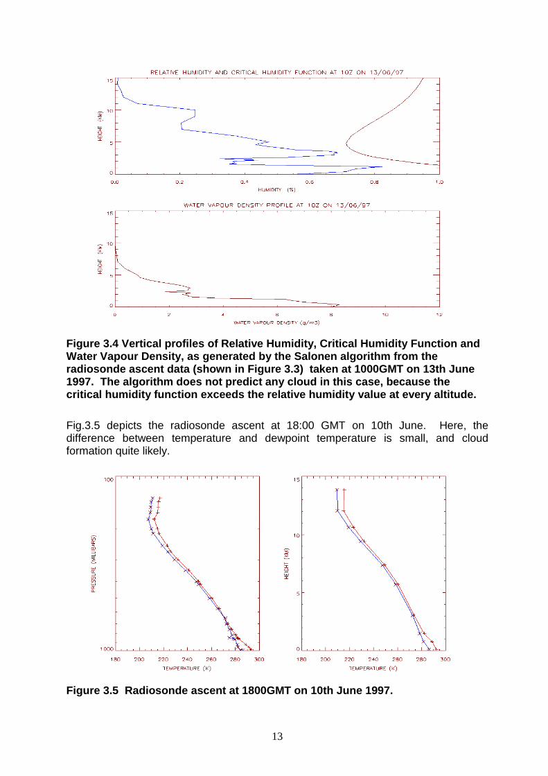
Fig.3.3 shows data from a typical radiosonde ascent where the vertical profiles of atmospheric temperature and dewpoint temperature are plotted against both pressure and altitude (temperature is shown in red and dewpoint temperature in blue), for the radiosonde ascent at 10:00 GMT on 13th June 1997. At the ground, atmospheric temperature is 5 K higher than the dewpoint temperature, and the difference between the two increases with altitude. In such conditions, the atmosphere is ‘dry’ (low relative humidity) and convectively stable, so that no clouds should be formed. Fig.3.4 shows that the relative humidity derived from this ascent is lower than the critical humidity function at each height, and so the algorithm does not generate any cloud from this ascent. The water vapour density profile is included in Fig.3.4 for completeness.

Figure 3.3 Radiosonde ascent from 1000GMT on 13th June 1997. The red trace shows ambient air temperature and the blue shows dewpoint temperature. The graph on the left shows the vertical profile with respect to atmospheric pressure, while the one on the right shows the profile with respect to altitude.

13

Figure 3.4 Vertical profiles of Relative Humidity, Critical Humidity Function and Water Vapour Density, as generated by the Salonen algorithm from the radiosonde ascent data (shown in Figure 3.3) taken at 1000GMT on 13th June 1997. The algorithm does not predict any cloud in this case, because the critical humidity function exceeds the relative humidity value at every altitude.

Fig.3.5 depicts the radiosonde ascent at 18:00 GMT on 10th June. Here, the difference between temperature and dewpoint temperature is small, and cloud formation quite likely.

Figure 3.5 Radiosonde ascent at 1800GMT on 10th June 1997.

14

Fig.3.6 shows that, for this ascent, the relative humidity is higher than the critical humidity function between 2km and 8km, and also shows the cloud liquid water content profile generated by the Salonen algorithm between these altitudes.

Figure 3.6 The results of the Salonen algorithm applied to the radiosonde ascent at 1800GMT on 10th June 1997. Here, a deep layer of cloud is predicted where the relative humidity exceeds the critical humidity function. The profile of cloud Liquid Water Content is also shown in the upper graph.

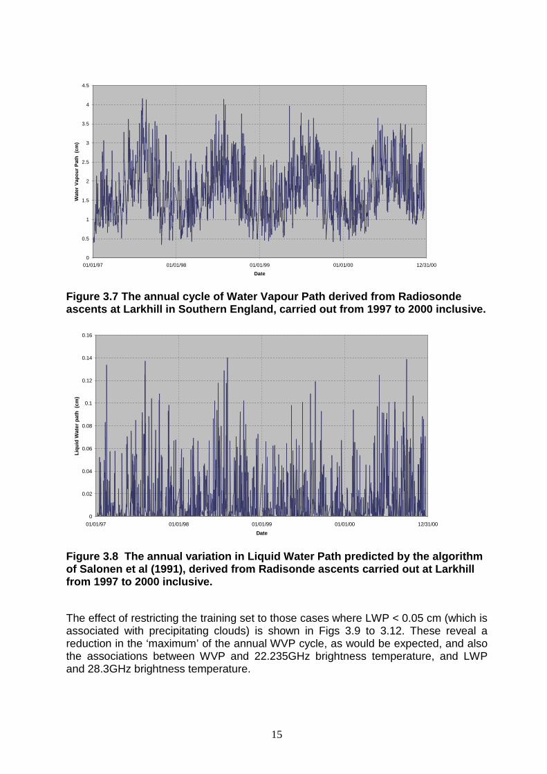
Figs. 3.7 and 3.8 show the results of using the Larkhill radiosonde data to compute WVP and LWP during the years 1997 to 2000 inclusive. In Fig.3.7, the annual variation of WVP between approximately 1cm (dry, Winter) and 4cm (humid, Summer) is apparent, which is in agreement with the findings of other experiments in the North Atlantic and Europe (Snider, 2000). An annual cycle is also discernible in the LWP values shown in Fig.3.8.

15

0

0.5

1

1.5

2

2.5

3

3.5

4

4.5

01/01/97 01/01/98 01/01/99 01/01/00 12/31/00

Date

Wat

er V

apo

ur

Pat

h (

cm)

Figure 3.7 The annual cycle of Water Vapour Path derived from Radiosonde ascents at Larkhill in Southern England, carried out from 1997 to 2000 inclusive.

0

0.02

0.04

0.06

0.08

0.1

0.12

0.14

0.16

01/01/97 01/01/98 01/01/99 01/01/00 12/31/00

Date

Liq

uid

Wat

er p

ath

(cm

)

Figure 3.8 The annual variation in Liquid Water Path predicted by the algorithm of Salonen et al (1991), derived from Radisonde ascents carried out at Larkhill from 1997 to 2000 inclusive.

The effect of restricting the training set to those cases where LWP < 0.05 cm (which is associated with precipitating clouds) is shown in Figs 3.9 to 3.12. These reveal a reduction in the ‘maximum’ of the annual WVP cycle, as would be expected, and also the associations between WVP and 22.235GHz brightness temperature, and LWP and 28.3GHz brightness temperature.

16

0

0.5

1

1.5

2

2.5

3

3.5

4

4.5

01/01/97 01/01/98 01/01/99 01/01/00 12/31/00

Date

Wat

er V

apo

ur

Pat

h (

cm)

Figure 3.9 Water vapour paths used in the training set after removal of values associated with precipitating cloud.

0

0.01

0.02

0.03

0.04

0.05

0.06

01/01/97 01/01/98 01/01/99 01/01/00 12/31/00

Date

Liq

uid

Wat

er p

ath

(cm

)

Figure 3.10 Liquid water paths used in the training set after removal of values associated with precipitating clouds (i.e., LWP > 0.05 cm have been excluded).

17

0

10

20

30

40

50

60

70

80

01/01/97 01/01/98 01/01/99 01/01/00 12/31/00

Date

Bri

gh

tnes

s T

emp

erat

ure

(K

)

Figure 3.11 Brightness temperatures at 22.235 GHz calculated from the Radiosonde Training Set. The annual cycle is comparable with the Water Vapour Path data in Fig. 3.9.

0

10

20

30

40

50

60

01/01/97 01/01/98 01/01/99 01/01/00 12/31/00

Date

Bri

gh

tnes

s T

emp

erat

ure

(K

)

Figure 3.12 Brightness Temperatures at 28.3 GHz calculated from the Radiosonde Training Set. The annual cycle is consistent with the cycles of Water Vapour Path and Liquid Water Path shown in Figs. 3.10 and 3.11.

18

3.5 Transfer function retrievals. The 4-year training set was used to obtain the following transfer functions by multiple linear regression.

LWP = -0.0126 – 0.0008 BT22 + 0.0025 BT28 WVP = 0.0350 + 0.0737 BT22 – 0.0394 BT28

Each of these equations describes an inclined planar surface in a three dimensional co-ordinate system, with axes (BT22, BT28, WVP) or (BT22, BT28, LWP). When brightness temperature measurements from the radiometers, BT22 and BT28, are used in the Transfer Functions, the estimated values of WVP and LWP will lie on this surface. However, the input data from the Training Set is scattered above and below the surface. This scatter represents the errors on the estimates of WVP and LWP (referred to as the Retrieval Accuracy) and can be measured by applying the Transfer Functions to the brightness temperatures used in the Training Set, then analysing the difference between the input and retrieved values of WVP & LWP. The entire procedure is illustrated in Fig. 3.13.

Figure 3.13 Schematic diagram of the stages involved in constructing a Training Set from radiosonde data, deriving the Transfer Functions and estimating their Retrieval Accuracy.

(WVD = atmospheric Water Vapour Density; LWC = cloud Liquid Water Content; WVP = Water Vapour Path; LWP = Liquid Water Path; Liebe refers to Liebe Millimetre-wave Propagation Model).

The differences between input and retrieved WVP & LWP are shown in Figs.3.14 and 3.15. In both cases, the Retrieval Accuracy is given by the standard deviation. (Note that this means the retrieved LWP can sometimes be negative). Finally, the procedure was extended to incorporate future measurements to be made by a 37GHz radiometer. A 3-frequency (22/28/37) retrieval algorithm was developed, which should provide more accurate estimates of LWP. Also, an

19

additional 2-frequency (22/37) retrieval algorithm was developed so that if either the 28 or 37GHz radiometers fails, continuous LWP estimates can be continued. Retrieval Accuracies for each of our frequency combinations are listed in Table 3.1, where the figures reported by previous experimenters are given for comparison.

Location WVP Retrieval Accuracy (CM)

LWP Retrieval Accuracy (CM)

GUIRAUD (1979) 0.1 GAO (1992) 0.1 SCHIAVON (1993) MID-LATITUDE SUMMER 0.12 0.007

SUBARCTIC WINTER 0.05 0.007 ROCKEN (1993) 0.1 Not given LESHT (1996) OKLAHOMA WINTER 0.1 Not given

OKLAHOMA SUMMER 0.1 Not given STEINHAGEN (1998)

0.1 Not given

GÜLDNER (1999) EUROPE WINTER 0.3 Not given EUROPE SUMMER 0.5 Not given

SIMPSON (2001) CHILBOLTON 22,28 GHz 0.083 0.0018 CHILBOLTON 22,37 GHz 0.076 0.0017 CHILBOLTON 22,28,37

GHz 0.042 0.0016

Table 3.1 Comparison of retrieval accuracies (quoted in standard deviations) reported by various experimenters.

-0.5

-0.4

-0.3

-0.2

-0.1

0

0.1

0.2

0.3

0.4

0.5

01/01/97 01/01/98 01/01/99 01/01/00 12/31/00

Date

Rad

iso

nd

e W

VP

- E

stim

ated

WV

P (

cm)

Figure 3.14 The difference between WVP obtained from Radiosonde analysis, and WVP estimated by applying the Transfer Function to the corresponding Brightness Temperatures.

20

-0.02

-0.015

-0.01

-0.005

0

0.005

0.01

0.015

0.02

0.025

0.03

01/01/97 01/01/98 01/01/99 01/01/00 12/31/00

Date

Rad

ioso

nd

e L

WP

- E

stim

ated

LW

P (

cm)

Figure 3.15 The difference between LWP obtained from Radiosonde analysis, and LWP estimated by applying the Transfer Function to the corresponding Brightness Temperatures.

3.6 Deriving atmospheric properties from Radiosonde data.

3.6.1 Water Vapour Pressure (Goff & Gratch, 1946).

Given the surface air temperature, T0, and dewpoint temperature TD(h) at each height h If T0 >= 273.16 K the vapour pressure over water is given by

( ){ }[ ] ( ) ( )

+

−−=

hT

TLog

hT

ThTeLog

D

S

D

SDw 1010 02808.5190298.7

( )

−−

−

− 11010*3816.11344.11

7 S

D

T

hT

( ) ( )wshT

T

eLogD

S

10

149149.33 11010*1328.8 +

−+

−−

−

where ew(TD(h)) is vapour pressure over water at height h (mb). TD(h) is dew point temperature at height h (K). TS is 373.16 K.

ews is 1023.246 mb. If T0 < 273.16 K the vapour pressure over ice is given by

( ){ }[ ] ( ) ( )

−

−−=

hT

TLog

hT

ThTeLog

D

I

D

IDi 1010 56654.3109718.9

21

( ) ( )iII

D eLogT

hT101876793.0 +

−+

where ei(TD(h)) is vapour pressure over ice at height h (mb). TI is 273.16 K. eiI is 6.1071 mb. 3.6.2 Air Density.

Given atmospheric pressure p (h) in mb and air temperature T(h) in K, the air density in kg/m3 is given by

( ) ( )( )

=hT

hph 34838.0ρ

3.6.3 Water Vapour Mixing ratio.

Given water vapour pressure e(TD(h)) in mb and atmospheric pressure p(h) in mb, the water vapour mixing ratio is given by

( )( )( )( )[ ]hTehp

hTehr

D

D

−=

)(

62197.0)(

3.6.4 Water Vapour Density.

Given the water vapour mixing ratio r(h) and air density ρ (h) in kg/m3, the water vapour density ρ w(h) is given by

( ) ( )( ) ( )hhr

hrhw ρρ

+

=1

3.6.5 Relative Humidity.

The relative humidity (RH) is defined as the ratio of the water vapour mixing ratio, r(h), to its saturation value, rs(h), at the same temperature and pressure.

( )( )

( )( )s

Diw

s e

hTe

Tphr

hrRH ≈=

,,

where T(h) is the air temperature at height h in Centigrade. eiw(TD(h)) is vapour pressure (mb) over ice or water at height h. es is the saturated vapour pressure over water given by the formula (Bolton, 1980) [“A Short Course in Cloud Physics”, Rogers and Yau, 1989, page 16]

( )( )

+×=

hT

hTes 5.243

67.17exp112.6

3.6.6 Cloud Liquid Water Content (Salonen, 1991).

The following model is illustrated for a standard atmospheric profile in Figs.3.1

22

and 3.2

The critical humidity function, Uc, is calculated at each altitude with the formula ( ) ( )[ ]5.0111 −+−−= σβσασcU

where α=1, β = √3, σ is the ratio of the atmospheric pressure at each height to surface pressure.

Cloud is assumed to occur at each altitude where the relative humidity is greater than Uc. This method is illustrated in Fig. 3.1, using a simulation of a standard atmospheric profile. Where cloud occurs, the liquid water content, w (g/m3), as a function of temperature t (oC), and height from cloud base hc, is given by

( ) ( )tph

hctww w

a

r

c

+= 10

where a = 1.4 is the parameter for height dependence.

c = 0.041 /oC is the parameter for temperature dependence. w0 = 0.14 g/m3 is the liquid water content, if hc = hr = 1.5 km at 0oC (i.e. at cloud base).

pw(t) is the liquid water fraction, approximated by pw(t) = 1 if 0oC < t pw(t) = 1+ t/20 if -20oC < t < 0oC pw(t) = 0 if t < -20oC

23

4 RESULTS. Two RCRU radiometers at Chilbolton have been measuring sky brightness temperature since 14th February 2001, a third was added during May 2002; the retrieval algorithm described in section 3 has been applied to those measurements to generate water vapour path (WVP) and liquid water path (LWP) estimates. The measurements, and the estimated products, have subsequently been compared with: • Predictions of clear-sky Brightness Temperatures and WVP estimated using the

Liebe MPM method, taking input data from ground-based meteorological instruments;

• Brightness Temperatures and WVP estimated from Larkhill radiosonde data; • Observations made with the ESA Multi-frequency radiometer (MFR); • GPS WVP estimates supplied by the University of Bath.

4.1 Calibration of RCRU microwave radiometers, and sources of experimental error.

Nine calibrations were carried out at regular intervals during the period February to June 2001; there were additional calibrations whenever changes were made to the instrument and its systems. The calibration method was tested to ensure its reproducibility, and tests using the ambient load were carried out to monitor receiver stability.

During calibration measurements it was found that both the 22.235GHz and the 28.8GHz receiver output voltages were stable to +/-0.02V while pointing at the cold load (77K), and +/-0.01V when pointing at the hot load (293K). This corresponds to an uncertainty of +/-0.7K when deriving brightness temperature from the radiometer output voltages. The variations are due to small drifts in receiver stability and to the presence of standing waves between the calibration antenna horn and the liquid nitrogen surface of the cold load. They result in uncertainties of +/-0.002cm (20g/m2) and +/-0.35 mm when deriving LWP and WVP respectively. From the history of clear-sky observations in 2001, three periods of different, but steady, calibrations are evident. The first period runs from the beginning of operations up to 20th March. The second begins on 21st March, when modifications to the data acquisition system (extra cable) caused a change in the output voltage of the 28GHz radiometer. The new calibration is steady until 19th April, when the 22GHz radiometer performance began to be adversely affected by cyclic increases (linked to solar heating) of the ambient temperature within the Receiver Cabin. The radiometers incorporate thermostatically controlled heaters designed to maintain the receiver electronics at a steady operating temperature. However, when the ambient temperature of the building rose above a certain point, the radiometer electronics could not lose heat quickly enough, and so the receiver response was not stable. This problem was dealt with at first by using a fan to cool the radiometer electronics, and then later by upgrading the cabin’s air-conditioning units to eliminate diurnal temperature variations. By comparing the radiometer estimates

24

of WVP with the values derived from GPS data by the University of Bath, we were able to verify that the radiometers had started to overestimate WVP when the units began to overheat, and also that the remedial action had cured the problem. The ambient temperature within the cabin was initially brought back under control on 14th May; the stability of the radiometers was checked, and they were re-calibrated. Since then, there have been no major changes to the instrument calibrations. It is intended that at least one calibration will be performed every two weeks.

4.1.1 Offset caused by dielectric lens in radiometer horn antenna.

Each radiometer antenna contains a dielectric lens designed to ensure uniform phase at the aperture. The lens material in the 22GHz antenna is Polypropylene, in the 28GHz and 37GHz antennas it is Polyethylene. As the antennas are quite large, it is not possible to incorporate them in the calibration procedure. Instead, a method to compensate for the error introduced by the additional path loss has been established.

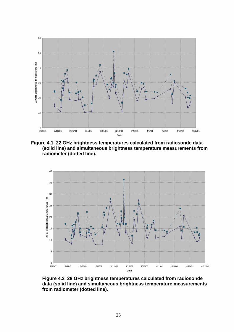
Figs. 4.1 and 4.2 illustrate the comparison between radiometer and radiosonde measurement based brightness temperatures for suitable sky conditions in the first third of 2001. These graphs reveal a clear qualitative correlation between the brightness temperatures from the radiometers and from the radiosondes. However, both radiometer values appear to be high.

The error introduced by each lens has been estimated by comparing the brightness temperatures measured with the radiometers, and those estimated from Larkhill radiosonde data when atmospheric conditions are homogenous (that is when skies are clear of liquid water bearing clouds, or the cloud cover is thin and uniform). For the purposes of this comparison we have selected periods when the measured sky brightness temperature at 28 GHz was 40K or lower. (This corresponds to integrated atmospheric path loss of <0.7dB) Radiometer brightness temperatures are plotted against coincident radiosonde-based estimates in Figs. 4.3 and 4.4.

Our current best estimates of the brightness temperature offsets caused by the presence of the lenses, are 6K at 22 GHz, and 4K at 28 GHz; these correspond to an insertion loss in each lens of 0.1 dB and 0.065 dB respectively. The offsets reduce as brightness temperature increases; a linear relationship between brightness temperature offset and observed brightness temperature has been established which enables corrections to be applied to all measured data.

25

0

10

20

30

40

50

60

2/11/01 2/18/01 2/25/01 3/4/01 3/11/01 3/18/01 3/25/01 4/1/01 4/8/01 4/15/01 4/22/01

Date

22 G

Hz

Bri

gh

tnes

s T

emp

erat

ure

(K

)

Figure 4.1 22 GHz brightness temperatures calculated from radiosonde data

(solid line) and simultaneous brightness temperature measurements from radiometer (dotted line).

0

5

10

15

20

25

30

35

40

2/11/01 2/18/01 2/25/01 3/4/01 3/11/01 3/18/01 3/25/01 4/1/01 4/8/01 4/15/01 4/22/01

Date

28 G

Hz

Bri

gh

tnes

s te

mp

erat

ure

(K

)

Figure 4.2 28 GHz brightness temperatures calculated from radiosonde data (solid line) and simultaneous brightness temperature measurements from radiometer (dotted line).

26

0

10

20

30

40

50

60

70

0 10 20 30 40 50 60 70

22 GHz Brightness Temperature from Radiosonde (K)

22 G

Hz

Bri

gh

tnes

s T

emp

erat

ure

fro

m R

adio

met

er (

K)

Figure 4.3 Radiometer vs radiosonde brightness temperatures at 22 GHz during clear sky conditions. The intercept provides an estimate of the offset caused by the radiometer antenna lens.

0

10

20

30

40

50

60

70

0 10 20 30 40 50 60 70

28 GHz Brightness Temperatures from Radiosonde (K)

28 G

Hz

Bri

gh

tnes

s T

emp

eera

ture

s fr

om

Rad

iom

eter

(K

)

Figure 4.4 28 GHz radiometer brightness temperature versus radiosonde brightness temperature during clear sky conditions. The intercept provides an estimate of the offset caused by the radiometer antenna lens.

27

0

1

2

3

4

0 1 2 3 4

WVP (cm) derived from Radiosonde Ascents

WV

P (

cm)

der

ived

fro

m U

nco

rrec

ted

Rad

iom

eter

dat

a.

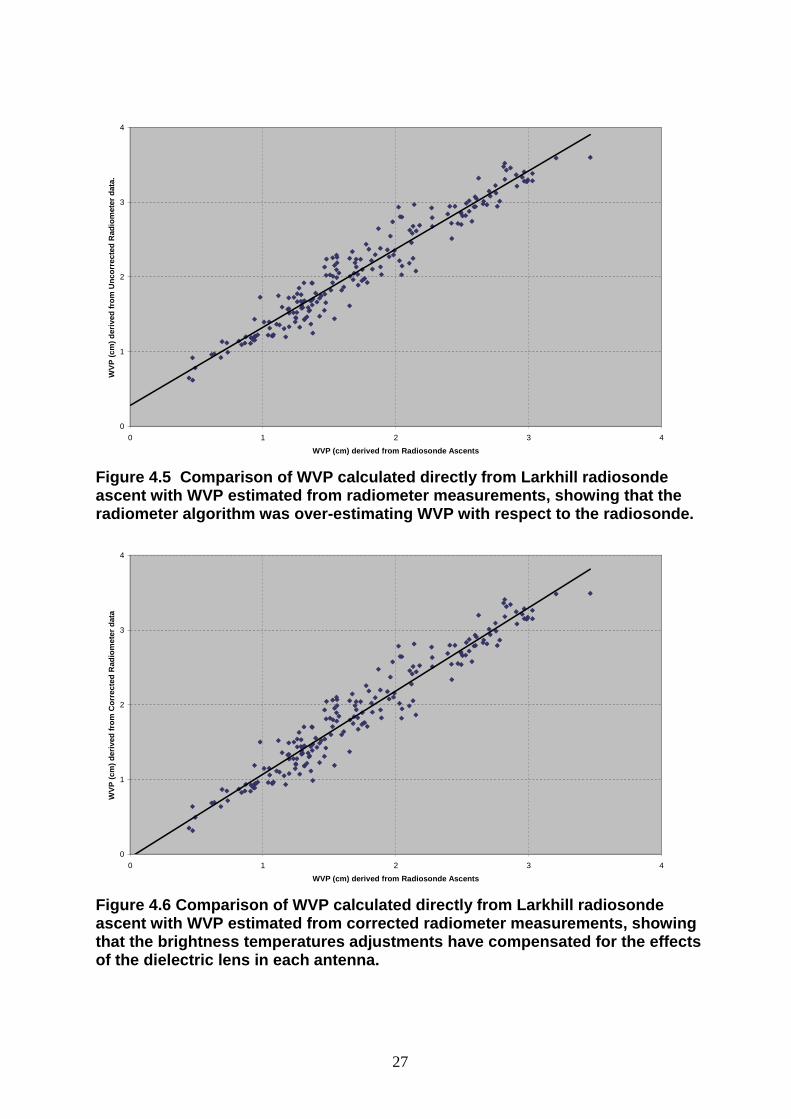
Figure 4.5 Comparison of WVP calculated directly from Larkhill radiosonde ascent with WVP estimated from radiometer measurements, showing that the radiometer algorithm was over-estimating WVP with respect to the radiosonde.

0

1

2

3

4

0 1 2 3 4

WVP (cm) derived from Radiosonde Ascents

WV

P (

cm)

der

ived

fro

m C

orr

ecte

d R

adio

met

er d

ata

Figure 4.6 Comparison of WVP calculated directly from Larkhill radiosonde ascent with WVP estimated from corrected radiometer measurements, showing that the brightness temperatures adjustments have compensated for the effects of the dielectric lens in each antenna.

28

In Figs. 4.5 and 4.6, WVP obtained directly from the radiosonde ascent data is compared with WVP estimates calculated by applying the Transfer Functions to the radiometer measurements, both before and after the radiometer brightness temperatures were corrected for the effects of the dielectric lenses. In the first case (Fig.4.5), the mean value of radiometer-estimated WVP differs from the radiosonde measurement. In the second case (Fig. 4.6), it is apparent that adjusting the radiometer Brightness Temperatures as described above, compensates for the effect of the lens to within the expected accuracy.

4.2 Validation of Measurements. When there is no cloud in the sky, radiometer measurements can be compared with predictions made by using the Liebe Millimetre-Wave Propagation Model (MPM) together with appropriate meteorological inputs. The MPM predictions are normally based on surface measurements of pressure, temperature and dew-point temperature which are recorded continuously at Chilbolton; these can be enhanced by using radiosonde data collected at Larkhill to provide additional information about the vertical profiles of water vapour and temperature. Predictions made from the surface-only measurements assume that the vertical profile of water vapour decreases exponentially with altitude. Water vapour scale height is estimated from radiosonde ascent data, as described in section 4.2.1.

29

4.2.1 The scale height of water vapour in Southern England. An exponential profile of water vapour can be written as:

( )

−=

S

hWhW exp0

where: W(h) is the water vapour density (g/m3) at altitude h (km), W0 is the water vapour density (g/m3) at the Earth’s surface, S is the scale height (km).

Water vapour decreases rapidly with altitude when S is small, and more slowly when S is large.

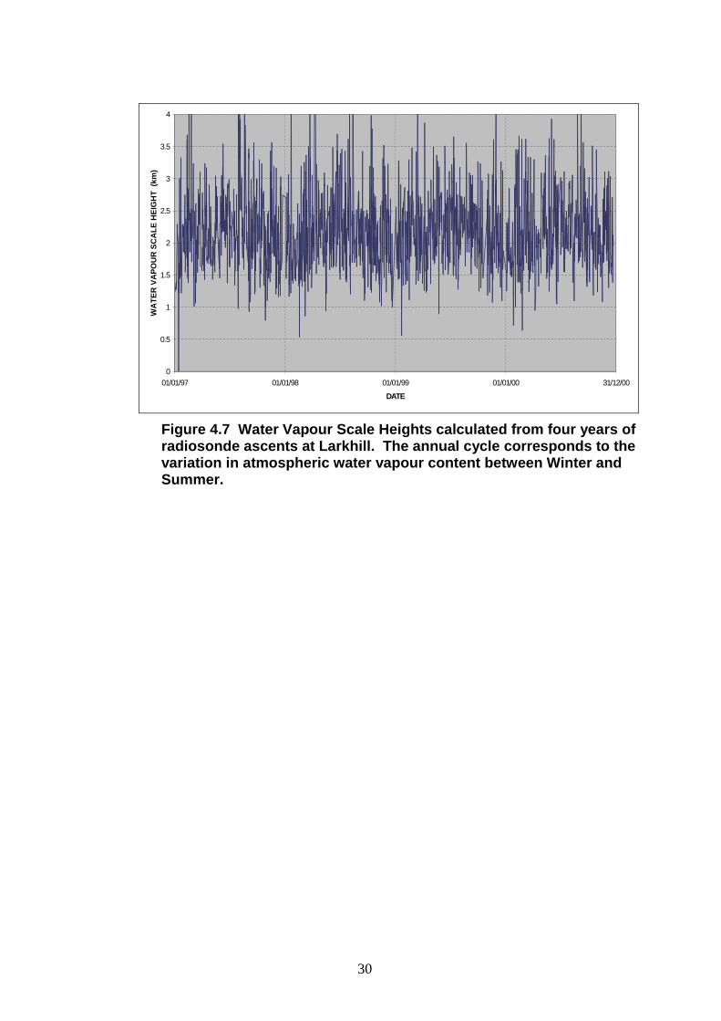
Examples of typical water vapour density profiles determined from radiosonde ascents are shown in Figs. 3.4 and 3.6. Most of the radiatively significant water vapour occurs in the lower troposphere, so that an estimate of water vapour scale height made using data from that region is more representative of the conditions that dominate the radiometer response. For this study, water vapour scale height has been determined from radiosonde profiles by fitting an exponential to the water vapour density values from the lowest 6km of data, and then assessing the point where W(h) = W'0exp(-1). The scale height S is equal to the altitude at that point, h. (W'0 is the surface value of water vapour density derived from an exponential fit to the radiosonde data). Scale heights that have been determined from the radiosonde ascents used for the Training Set are shown in Fig.4.7; the difference between Winter and Summer atmospheres is apparent.

30

0

0.5

1

1.5

2

2.5

3

3.5

4

01/01/97 01/01/98 01/01/99 01/01/00 31/12/00

DATE

WA

TE

R V

AP

OU

R S

CA

LE

HE

IGH

T (

km)

Figure 4.7 Water Vapour Scale Heights calculated from four years of radiosonde ascents at Larkhill. The annual cycle corresponds to the variation in atmospheric water vapour content between Winter and Summer.

31

4.2.2 A comparison between measured and predicted brightness temperature. 20th June 2001 was a day in which periods of cloud free skies provided an opportunity to demonstrate the effectiveness of Liebe's MPM procedures. This day was mainly clear of cloud at Chilbolton apart from the passage of a cold front that crossed southern UK during the afternoon. Cold fronts normally consist of a narrow band of deep, dense rain clouds, typically preceded by clear-sky or fairweather-cumulus cloud, and followed by the gradual clearing of low-altitude cloud. Pictures from the Chilbolton cloud camera show changes in the sky during 20th June, that confirm this (see Figs. 4.8a and 4.8b). The radiometer brightness temperatures for 20th June are shown in Fig.4.9. In addition we have plotted hourly clear-sky predictions of brightness temperature made using the surface meteorological measurements together with water vapour scale heights derived from radiosonde ascents at 0500, 1000, 1200 and 1400 GMT. Predictions based on the radiosonde measurements alone are also included. It can be seen that radiometer measurements at 22 GHz are in better agreement with the radiosonde based estimates. This is to be expected because the radiosonde is able to detect the build up of water vapour in the upper atmosphere that precedes the formation of the clouds. From the sky camera pictures we can see that cloud begins to occur at about 12:30 GMT, this corresponds to an increase in brightness temperature at 28.8 GHz.

32

10AM

12noon

2PM

11AM

1PM

3PM

Figure 4.8a Chilbolton Cloud-camera photos from 20th June 2001, illustrating the arrival of a cold front between 12 noon and 1pm.

33

4PM

6PM

8PM

5PM

7PM

Figure 4.8b Chilbolton Cloud-camera photos from 20th June 2001, illustrating the clearance of the skies after the passage of a cold front.

34

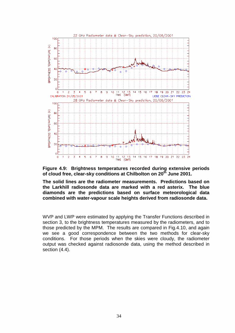
Figure 4.9: Brightness temperatures recorded during extensive periods of cloud free, clear-sky conditions at Chilbolton on 20th June 2001.

The solid lines are the radiometer measurements. Predictions based on the Larkhill radiosonde data are marked with a red asterix. The blue diamonds are the predictions based on surface meteorological data combined with water-vapour scale heights derived from radiosonde data.

WVP and LWP were estimated by applying the Transfer Functions described in section 3, to the brightness temperatures measured by the radiometers, and to those predicted by the MPM. The results are compared in Fig.4.10, and again we see a good correspondence between the two methods for clear-sky conditions. For those periods when the skies were cloudy, the radiometer output was checked against radiosonde data, using the method described in section (4.4).

35

Figure 4.10: WVP (top) & LWP(bottom) estimated from measurements made with the radiometers, radiosondes, and surface met. instruments, on 20th June 2001 at Chilbolton. The solid lines are the estimates from the Transfer Functions applied to the radiometer data. Similarly, the blue diamonds are estimated from the predictions for clear-sky conditions shown in Fig 4.9. The estimates based on Larkhill radiosonde data are marked with a red asterix.

4.3 Brightness Temperature estimates from radiosonde measurements.

The Larkhill radiosonde data has been used as input to the Liebe MPM prediction model for the estimation of sky brightness temperature. In Figs 4.9 and 4.10, values of WVP & LWP obtained from radiosonde data are shown by a red asterix. The general agreement between all three methods when estimating clear-sky values is apparent, especially for the values of LWP during the morning. In the afternoon when cloud moves across, the LWP estimate from the surface meteorological data does not respond because the calculation is based on the assumption of cloud free skies. The radiosonde-based values of liquid water do include the cloud because the Salonen estimator of cloud is applied (as described in section 3.4).

36

During the day, instruments at Chilbolton recorded windspeeds of approximately 18 km/hr from the West, which suggests that the apparent time-lag of one hour between the radiosonde and radiometer LWP estimates corresponds to the time taken for clouds to drift from Larkhill to Chilbolton.

4.4 Comparison of water vapour path estimates from radiometer observations, GPS receivers, and radiosonde measurements.

The Department of Electronic and Electrical Engineering at the University of Bath provided us with estimates of Integrated Precipitable Water Vapour (IPWV), calculated for the atmosphere over Chilbolton from measurements of GPS satellite signals during the 6 month period from the beginning of March to the beginning of September in 2001. These estimates are spaced at 5-minute intervals, and by suitable averaging of the radiometer outputs we are able to compare estimates of columnar atmospheric water vapour from independent sources. The comparisons are shown in Figures 4.11a and 4.11b, time-series of WVP estimates for March to September 2001. For good measure we have also plotted WVP obtained directly from the Larkhill Radiosonde data. The overall correspondence between the three independent estimates is clear, but closer examination reveals differences in the finer detail. However, on inspection we have been able to attribute these differences to the following causes:

(i) Differences in the measurement technique, such as : the distance between the Larkhill Radiosonde site and the Chilbolton observatory; the different ‘field-of-view’ of the radiometers and the GPS satellites & receiver; and the lack of 24 hour coverage in the Radiosonde data. (ii) Different sources of measurement error, such as condensation around the radiometers. (iii) Radiometer failure, such as overheating of the instrument electronics.

37

Figure 4.11a Time series of WVP estimated by three independent techniques, March 2001 to May 2001 inclusive.

Figure 4.11b Time series of WVP estimated by three independent techniques, June 2001 to August 2001 inclusive. A statistical summary of the comparison is illustrated in Figure 4.12. This shows histograms of WVP estimates, expressed as a percentage of the total number of samples obtained by each of the three techniques. On average, there is a 15% difference between the GPS and Radiometer estimates of WVP. Note that the Radiosonde measurements are taken at approximately the same time on each day(usually one early in the morning, and one near midday or early in the afternoon). So as well as being prone to greater variation because there are far fewer samples than the other two methods, the Radiosonde data

38

shows signs of a bi-modal distribution in the histogram.

Figure 4.12 Histograms of WVP estimated by 3 independent techniques.

‘GPS’ values were derived from Global Positioning Satellite data. ‘RMR’ estimated from radiometer brightness temperature measurements, ‘RS’ values from direct measurement using radiosonde ascent data.

Finally, Figure 4.13 shows a direct comparison between the GPS and Radiometer estimates of WVP for the period 7th to 27th August 2001. This period was selected because there is a minimum of ‘outside interference’ by the error sources described above. In this Figure, the outlying data corresponds to Radiometer observations adversely affected by rainfall. The R2 correlation coefficient associated with the best-fit line in the figure is 0.95, and we take this to indicate that the radiometer retrieval algorithm, in the absence of contaminated data, is performing accurately and reliably. Strictly speaking, this conclusion applies only to the WVP retrieval, and may not hold for the LWP retrieval. However, it is fair to say that the retrieval technique is sound, at least until such time as we are able to compare radiometer-retrieved LWP with independently measured values.

39

Figure 4.13 A direct comparison of WVP estimated by the GPS and the Radiometer retrieval algorithms, covering the period from 7th August 2001 to 27 August 2001.

40

4.5 Clouds and Rain. Here we look at the radiometer measurements under cloudy conditions.

Figure 4.14: Cloud radar time-series showing passage of cloud and rain over Chilbolton on 14th June 2001.

Rainfall (approximately 10mm/hr) was recorded by surface gauges between 1500 & 1530 UTC, and between 1800 & 2100 UTC.

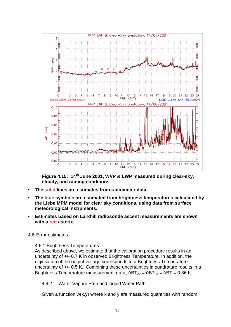
The general conditions at Chilbolton on 14th June 2001 are shown by the time-series data from the vertically pointing 94 GHz cloud radar, shown in Fig 4.14. Clear-skies in the morning were followed by a build-up of cloud in the afternoon, and then rain just after 1500 and 1800. The corresponding changes in WVP & LWP are shown in Fig 4.15. Once again, there is reasonable agreement between the clear-sky values estimated by the three methods, and good agreement between the radiometer and radiosonde estimates during the cloudy periods. LWP derived from the radiosondes at Larkhill would not necessarily be the same as LWP derived from the radiometers. On 14th June, wind direction was mainly from the South, and since Larkhill is to the West of Chilbolton, the radiosonde would not have seen the same clouds that passed over Chilbolton. Liquid water content is naturally inhomogenous and variable, both spatially and temporally even for stratus cloud (widespread, overcast conditions); so the distance between Larkhill and Chilbolton means that exact comparisons are rarely possible. However, atmospheric water vapour density does tend to be more homogenous over large distances, so it is encouraging to know that there is close agreement between the estimates of WVP under different conditions.

41

Figure 4.15: 14th June 2001, WVP & LWP measured during clear-sky, cloudy, and raining conditions.

• The solid lines are estimates from radiometer data.

• The blue symbols are estimated from brightness temperatures calculated by the Liebe MPM model for clear sky conditions, using data from surface meteorological instruments.

• Estimates based on Larkhill radiosonde ascent measurements are shown with a red asterix.

4.6 Error estimates.

4.6.1 Brightness Temperatures. As described above, we estimate that the calibration procedure results in an uncertainty of +/- 0.7 K in observed Brightness Temperature. In addition, the digitisation of the output voltage corresponds to a Brightness Temperature uncertainty of +/- 0.5 K. Combining these uncertainties in quadrature results in a Brightness Temperature measurement error, !BT22 = !BT28 = !BT = 0.86 K.

4.6.2 Water Vapour Path and Liquid Water Path

Given a function w(x,y) where x and y are measured quantities with random

42

measurement errors ! ! !x and y, the uncertainty in w. w is given by the formula

22

∂∂+

∂∂= y

y

wx

x

ww δδδ

So for Transfer Functions of the form w = ax + by where a and b are constants, an estimate of the error !w arising from uncertainties !x and !y is given by

( ) ( )22 ybxaw δδδ += Applying this to the 22 & 28 GHz Transfer Functions for WVP and LWP (chapter 3), the errors in Brightness Temperature measurements result in uncertainties of !WVP = 0.08 cm, and !LWP = 0.002cm (both to first significant figure). Finally, the uncertainties due to measurement error are combined in quadrature with the Transfer Function retrieval accuracies (section 3.5).

Table 4.1 shows the error estimates associated with different combinations of radiometer frequencies. For the 22/28 GHz combination used up until June 2002, the estimated error in WVP is 0.1cm, and in LWP it is 0.003cm (30 g/m2). Addition of the 37 Ghz radiometer reduces the estimated error in LWP to 0.0022cm (22 g/m2) By comparison, Crewell (1999) using cloud base height and temperature in a neural-network algorithm, reported LWP rms errors of ~20 g/m2. Table 4.1 Frequency Combination

Uncertainty (cm) due to Brightness Temperature measurement error

Retrieval Accuracy (cm)

Errror Estimate (cm)

! W V P ! L W P ! W V P ! L W P ! W V P ! L W P 22, 28 Ghz 0.08 0.0024 0.083 0.0018 0.1 0.0030 22, 37 GHz 0.07 0.0015 0.076 0.0017 0.1 0.0022 22,28,37GHz 0.20 0.0013 0.042 0.0016 0.2 0.0021

43

5 CONCLUSIONS

This report has described how microwave radiometers are being used to make multi-frequency measurements of sky brightness temperature; from those measurements we have shown how total water vapour path (precipitable water), and total liquid water path, can be estimated above the Chilbolton Observatory. The algorithm that has been developed to perform the inversion of the data is described together with estimates of the retrieval accuracy that is expected. Examples of retrievals performed on measured data have been compared with predictions based on surface and radiosonde measurements. These results confirm the effectiveness of the procedures being used.

44

6 REFERENCES

Bolton, D. (1980), “The computation of equivalent potential temperature”, Monthly Weather Review,, Vol.108, pages 1046-1053. Crewell, S., Löhnert, L., and Simmer, C., (1999), “Remote sensing of liquid water profiles using microwave radiometry”, Proceedings of Symposium in Remote Sensing of Cloud Parameters : Retrieval and Validation, International Research Centre of Telecommunication-Transmission and Radar, Delft University of Technology, October 1999. Goff, J.A. & Gratch, S., (1946), "Low-pressure properties of water from -160 to 212F", Trans. Amer. Soc. Heat and Vent. Engineering, Vol.52, pages 95-122. Güldner, J. and Spänkuch, D., (1999), “Results of year-round remotely sensed integrated water vapour by ground-based microwave radiometry”, Journal of Apllied Meteorology, Vol.38, pages 981-988. Liebe, H.J., (1989), “MPM – an atmospheric millimetre-wave propagation model.”, International Journal of Infrared and Millimetre Waves, Vol.10, pages 631-650. Matveev, L., (1984), “Cloud Dynamics”, D.Riedel Publishing Company, Dordrecht, page 340.

Rogers, R.R. and M.K.Yau, (1996), “A Short Course In Cloud Physics”, 3rd Edition, Butterworth Heinemann. Salonen, E., (1991), “New prediction method of cloud attenuation”, Electronics Letters, Vol.27, No.12, pages 1106-1108. Schiavon, D. and G.Solimini, (1993), “Performance analysis of a multi-frequency radiometer for predicting atmospheric propagation parameters”. Radio Science, Vol.28, No.1, pages 63-76. Snider, J.B., (2000), "Temporal Variability of Precipitable Water Vapour in the Northern Atlantic". IEEE Trans Geo & Remote Sensing, Vol.38, No 3, pages 1489-1491.