Embed Size (px)
Citation preview
SEISMIC FRAGILITY ASSESSMENT FOR REINFORCED CONCRETE
HIGH-RISE BUILDINGS
BY
JUN JI
AMR S. ELNASHAI
DANIEL A. KUCHMA
Report 07-14 September 2007
Mid-America Earthquake Center
Headquarter: University of Illinois at Urbana-Champaign

iii
Abstract
In contrast to the worldwide rapid growth of high-rise buildings, no probabilistic assessment
procedures have been proposed or developed for seismic risk evaluation of this special building
group. The new purpose of this report is to provide the earthquake engineering community with
an integrated probabilistic seismic fragility assessment framework and a reference application for
this special building population.
A complete methodology is presented for the seismic fragility assessment of reinforced concrete
high-rise buildings. The key steps of the methodology are illustrated through an example of the
fragility assessment of an existing 54-storey building with a dual core wall system. The set of
rigorously derived probabilistic fragilities are the first published for high-rise RC buildings, thus
they fill an important void in regional earthquake impact assessment in Metropolitan
communities. The inelastic dynamic analyses for the fragility assessments are undertaken using a
simplified lumped-parameter model that was derived from highly detailed FE models using
genetic algorithms. New definitions for performance limit states are based on the results of
detailed pushover analyses of a multi-resolution distributed finite element model that includes
shear-flexure-axial interaction effects. To develop the fragility relationships, more than two
thousand dynamic response history analyses were conducted. This study considered uncertainty
in structural material values as well as in seismic demand. Thirty natural and twenty artificial
strong motion records were selected for the analyses that would produce an appropriate range in
structural response parameters due to variation in magnitude, distance and site condition. The
overall approach is generic and can be applied to develop computationally efficient and
probabilistically based seismic fragility relationships for RC high-rise buildings of different
configurations.

iv
Acknowledgements
This study is a product of project EE-1 ‘Vulnerability Functions’ of the Mid-America Earthquake
Center. The MAE Center is an Engineering Research Center funded by the National Science
Foundation under cooperative agreement reference EEC 97-01785.
v
Table of Contents
List of Tables .......................................................................................................................... ix
List of Figures......................................................................................................................... xi
1. Introduction........................................................................................................................1
1.1 Significance....................................................................................................................1
1.2 Objectives ......................................................................................................................5
1.3 Organization of the Report.............................................................................................5
2. Seismic Fragility Assessment of RC High-rise Buildings...............................................8
2.1 RC High-rise Building Configuration and Design.........................................................8
2.1.1 High-rise Building Definition ...............................................................................9
2.1.2 Structural Types ....................................................................................................9
2.2 Seismic Design and Performance of RC High-rise Systems .......................................13
2.3 Requirements for Fragility Assessment .......................................................................16
3. Analytical Structural Modeling......................................................................................19
3.1 Literature Survey .........................................................................................................19
3.1.1 Material Properties..............................................................................................19
3.1.2 Structural Components .......................................................................................21
3.1.3 Seismic Analysis Approaches.............................................................................24
3.2 Material Constitutive Relationship ..............................................................................26
3.2.1 Concrete ..............................................................................................................26
3.2.2 Reinforcement Steel ...........................................................................................35
3.3 Beam-Column Members and Wall Panel ....................................................................36
3.3.1 Beam-Column Members.....................................................................................36
3.3.1.1 Beam Model with Fibered Sectional Approach......................................36
vi
3.3.1.2 ZEUS-NL Application ...........................................................................38
3.3.2 Structural Wall Panels.........................................................................................39
3.3.2.1 Macroscopic Model ................................................................................40
3.3.2.2 Microscopic Model .................................................................................42
3.3.2.3 VecTor2 Application ..............................................................................45
3.3.2.4 Necessity of Lumped-Parameter-Based Modeling .................................46
3.3.3 Wall-Frame Interaction.......................................................................................47
3.3.4 Verifications of Frame and Wall FEM Analysis Software.................................49
3.3.4.1 ZEUS-NL for Frame Analysis ................................................................49
3.3.4.2 VecTor2 for Wall Analysis.....................................................................50
3.4 Lumped-Parameter-Based Model Derivation ..............................................................57
3.4.1 Methodology.......................................................................................................59
3.4.2 Reference Building Selection .............................................................................63
3.4.3 Mass Simulation..................................................................................................64
3.4.4 Simplification Stage I Using Genetic Algorithm................................................65
3.4.4.1 ZEUS-NL Pushover Analysis of Full Model..........................................65
3.4.4.2 Construct Equivalent Wall Boundary Supports......................................68
3.4.4.3 Parametric Study with Genetic Algorithm..............................................69
3.4.5 Simplification Stage II Using Genetic Algorithm ..............................................76
3.4.5.1 VecTor2 Analysis Using Continuum FEM Model .................................76
3.4.5.2 Investigated Wall Lumped Modelling ....................................................78
3.4.5.3 Parametric Study with Genetic Algorithm..............................................78
3.4.6 Lumped Model Evaluation .................................................................................82
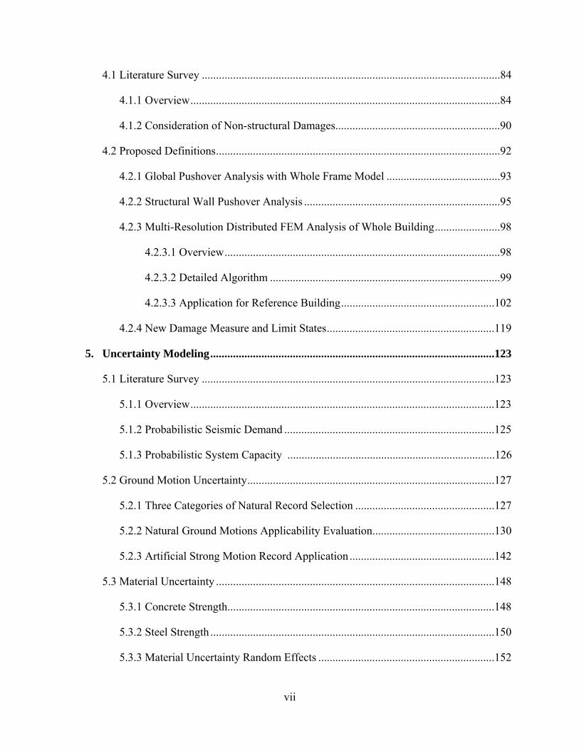
4. Limit States Definition.....................................................................................................84
vii
4.1 Literature Survey .........................................................................................................84
4.1.1 Overview.............................................................................................................84
4.1.2 Consideration of Non-structural Damages..........................................................90
4.2 Proposed Definitions....................................................................................................92
4.2.1 Global Pushover Analysis with Whole Frame Model ........................................93
4.2.2 Structural Wall Pushover Analysis .....................................................................95
4.2.3 Multi-Resolution Distributed FEM Analysis of Whole Building.......................98
4.2.3.1 Overview.................................................................................................98
4.2.3.2 Detailed Algorithm .................................................................................99
4.2.3.3 Application for Reference Building......................................................102
4.2.4 New Damage Measure and Limit States...........................................................119
5. Uncertainty Modeling....................................................................................................123
5.1 Literature Survey .......................................................................................................123
5.1.1 Overview...........................................................................................................123
5.1.2 Probabilistic Seismic Demand ..........................................................................125
5.1.3 Probabilistic System Capacity .........................................................................126
5.2 Ground Motion Uncertainty.......................................................................................127
5.2.1 Three Categories of Natural Record Selection .................................................127
5.2.2 Natural Ground Motions Applicability Evaluation...........................................130
5.2.3 Artificial Strong Motion Record Application ...................................................142
5.3 Material Uncertainty ..................................................................................................148
5.3.1 Concrete Strength..............................................................................................148
5.3.2 Steel Strength ....................................................................................................150
5.3.3 Material Uncertainty Random Effects ..............................................................152
viii
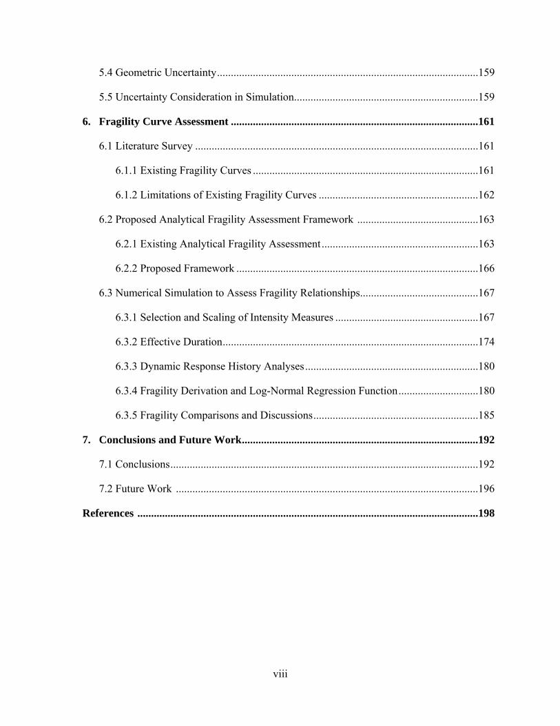
5.4 Geometric Uncertainty...............................................................................................159
5.5 Uncertainty Consideration in Simulation...................................................................159
6. Fragility Curve Assessment ..........................................................................................161
6.1 Literature Survey .......................................................................................................161
6.1.1 Existing Fragility Curves ..................................................................................161
6.1.2 Limitations of Existing Fragility Curves ..........................................................162
6.2 Proposed Analytical Fragility Assessment Framework ............................................163
6.2.1 Existing Analytical Fragility Assessment.........................................................163
6.2.2 Proposed Framework ........................................................................................166
6.3 Numerical Simulation to Assess Fragility Relationships...........................................167
6.3.1 Selection and Scaling of Intensity Measures ....................................................167
6.3.2 Effective Duration.............................................................................................174
6.3.3 Dynamic Response History Analyses...............................................................180
6.3.4 Fragility Derivation and Log-Normal Regression Function.............................180
6.3.5 Fragility Comparisons and Discussions............................................................185
7. Conclusions and Future Work......................................................................................192
7.1 Conclusions................................................................................................................192
7.2 Future Work ..............................................................................................................196
References ............................................................................................................................198
ix
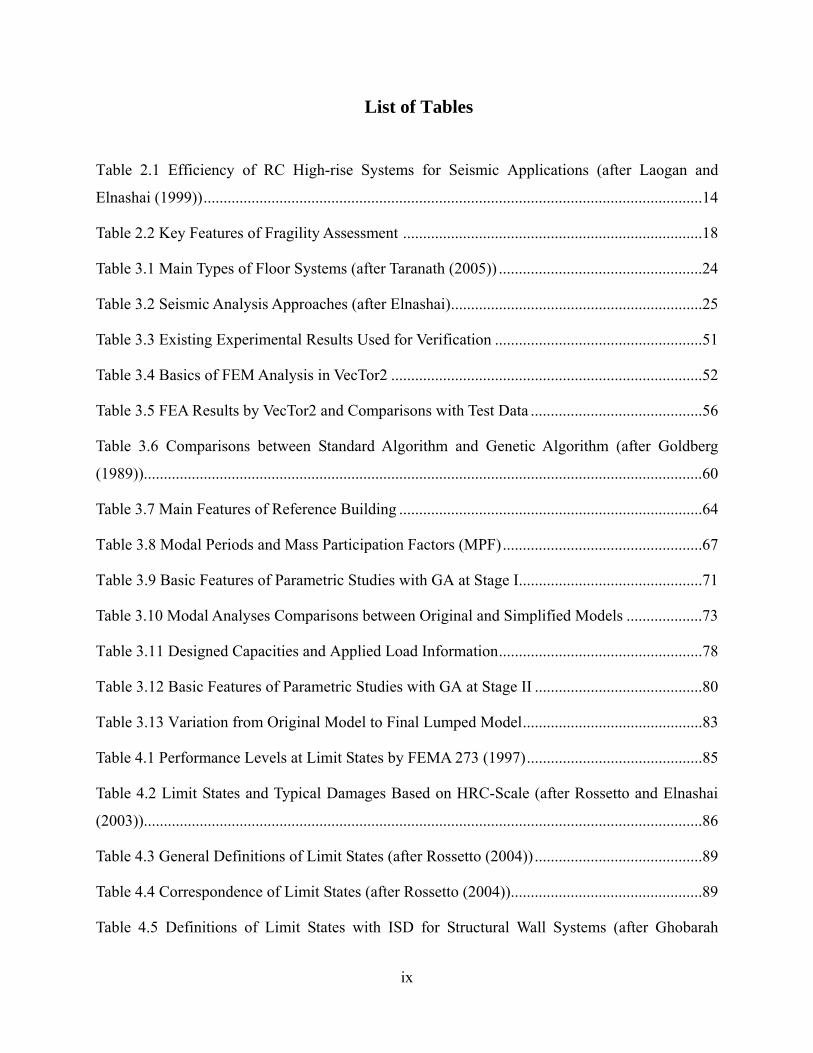
List of Tables
Table 2.1 Efficiency of RC High-rise Systems for Seismic Applications (after Laogan and
Elnashai (1999)).............................................................................................................................14
Table 2.2 Key Features of Fragility Assessment ...........................................................................18
Table 3.1 Main Types of Floor Systems (after Taranath (2005)) ...................................................24
Table 3.2 Seismic Analysis Approaches (after Elnashai)...............................................................25
Table 3.3 Existing Experimental Results Used for Verification ....................................................51
Table 3.4 Basics of FEM Analysis in VecTor2 ..............................................................................52
Table 3.5 FEA Results by VecTor2 and Comparisons with Test Data ...........................................56
Table 3.6 Comparisons between Standard Algorithm and Genetic Algorithm (after Goldberg
(1989))............................................................................................................................................60
Table 3.7 Main Features of Reference Building ............................................................................64
Table 3.8 Modal Periods and Mass Participation Factors (MPF)..................................................67
Table 3.9 Basic Features of Parametric Studies with GA at Stage I..............................................71
Table 3.10 Modal Analyses Comparisons between Original and Simplified Models ...................73
Table 3.11 Designed Capacities and Applied Load Information...................................................78
Table 3.12 Basic Features of Parametric Studies with GA at Stage II ..........................................80
Table 3.13 Variation from Original Model to Final Lumped Model.............................................83
Table 4.1 Performance Levels at Limit States by FEMA 273 (1997)............................................85
Table 4.2 Limit States and Typical Damages Based on HRC-Scale (after Rossetto and Elnashai
(2003))............................................................................................................................................86
Table 4.3 General Definitions of Limit States (after Rossetto (2004))..........................................89
Table 4.4 Correspondence of Limit States (after Rossetto (2004))................................................89
Table 4.5 Definitions of Limit States with ISD for Structural Wall Systems (after Ghobarah
x
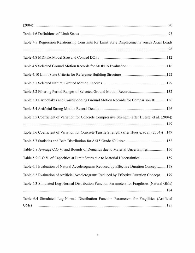
(2004)) ..........................................................................................................................................90
Table 4.6 Definitions of Limit States .............................................................................................93
Table 4.7 Regression Relationship Constants for Limit State Displacements versus Axial Loads
........................................................................................................................................................98
Table 4.8 MDFEA Model Size and Control DOFs ......................................................................112
Table 4.9 Selected Ground Motion Records for MDFEA Evaluation .........................................116
Table 4.10 Limit State Criteria for Reference Building Structure ...............................................122
Table 5.1 Selected Natural Ground Motion Records ...................................................................129
Table 5.2 Filtering Period Ranges of Selected Ground Motion Records.....................................132
Table 5.3 Earthquakes and Corresponding Ground Motion Records for Comparison III ...........136
Table 5.4 Artificial Strong Motion Record Details ......................................................................146
Table 5.5 Coefficient of Variation for Concrete Compressive Strength (after Hueste, et al. (2004))
......................................................................................................................................................149
Table 5.6 Coefficient of Variation for Concrete Tensile Strength (after Hueste, et al. (2004)) .149
Table 5.7 Statistics and Beta Distribution for A615 Grade 60 Rebar ...........................................152
Table 5.8 Average C.O.V. and Bounds of Demands due to Material Uncertainties ...................156
Table 5.9 C.O.V. of Capacities at Limit States due to Material Uncertainties............................159
Table 6.1 Evaluation of Natural Accelerograms Reduced by Effective Duration Concept .........178
Table 6.2 Evaluation of Artificial Accelerograms Reduced by Effective Duration Concept ......179
Table 6.3 Simulated Log-Normal Distribution Function Parameters for Fragilities (Natural GMs)
......................................................................................................................................................184
Table 6.4 Simulated Log-Normal Distribution Function Parameters for Fragilities (Artificial
GMs) ......................................................................................................................................185

xi
List of Figures
Figure 1.1 Distribution of High-rise Buildings in the World (© http://www.emporis.com, 2006) .2
Figure 2.1 Height Limit of High-rise Building................................................................................9
Figure 2.2 Concrete Systems Suitable for Buildings with Different Number of Stories (after Ali
(2001)) ...........................................................................................................................................11
Figure 2.3 General Fragility Assessment Framework....................................................................17
Figure 3.1 Typical Structural Wall Cross Sections ........................................................................22
Figure 3.2 Typical FEM Seismic Analysis Algorithm ...................................................................26
Figure 3.3 Concrete Responses to Compression Load (Mehta and Monteiro (1993)) ..................27
Figure 3.4 Typical Stress Strain Curves of Different f’c Levels (from Mendis (2003))................28
Figure 3.5 Enhancement Effects by Confining Pressures (from Candappa et al. (1999)).............28
Figure 3.6 Variations of Strength as a Function of Strain-rate: Crushing Strength for Concrete
(left) and Yield Strength for Steel (Right) (from Bruneau et al. (1998)) .......................................29
Figure 3.7 Compressive Constitutive Models Suitable for NSC: Popovics (1973) (Upper) and
Hognestad Parabola (Lower) .........................................................................................................30
Figure 3.8 Modified Popovics Constitutive Model Suitable for HSC (Collins and Porasz (1989))
........................................................................................................................................................30
Figure 3.9 Vecchio and Collins-Mitchell Tension Stiffening Response Models ...........................31
Figure 3.10 Mohr-Coulomb and Drucker-Prager Failure Criteria .................................................33
Figure 3.11 Multi-surface Plasticity Models for Concrete ............................................................34
Figure 3.12 Stress-strain Relationship of Reinforcing Steel..........................................................35
Figure 3.13 Configuration of Beam Using Timoshenko Beam Theory.........................................37
Figure 3.14 Construction of a Fiber Element (after Spacone et al. (1996))...................................37
Figure 3.15 Structural Wall Failure Modes (Top) and Cyclic Response (Bottom): Flexural (Left)
and Shear (Right) Modes (Paulay and Priestley, 1992) .................................................................39
xii
Figure 3.16 Macroscopic Structural Wall Models (after Vulcano (1992)) ....................................40
Figure 3.17 Macroscopic Structural Wall Models (after Ghobarah and Youseff (1999))..............42
Figure 3.18 Smeared Concrete Element Model.............................................................................43
Figure 3.19 Mohr’s Circle of Average Strains ...............................................................................44
Figure 3.20 Hysteretic Models for Concrete (after Palermo and Vecchio (2003)) ........................53
Figure 3.21 LSW1 Test Structure and Data vs. FEM Model and Analysis Results.......................56
Figure 3.22 MSW1 Test Structure and Data vs. FEM Model and Analysis Results .....................57
Figure 3.23 Equivalent Nonlinear Springs at Wall Joint ...............................................................59
Figure 3.24 Structure of Genetic Algorithm ..................................................................................61
Figure 3.25 Global Stick (Lumped) Model Derivation Using Genetic Algorithm........................62
Figure 3.26 Reference Building SAP2000 Model (Left), Half Plane View (Middle) and ZEUS-
NL Model (Right) .........................................................................................................................63
Figure 3.27 Lumped Mass Model in Selected Structure................................................................65
Figure 3.28 Structural Model in ZEUS-NL (a) and Typical Component Cross Sections (b ~ d)
........................................................................................................................................................66
Figure 3.29 First Five Natural Modal Shapes................................................................................67
Figure 3.30 Distributed Lateral Loads Following Mixed Modal Shape........................................68
Figure 3.31 Main Features in Simplified Model Stage I ...............................................................69
Figure 3.32 Pushover Response Comparisons between Original and Lumped Models ................74
Figure 3.33 Pushover Deformed Shape Comparisons at X Direction ...........................................74
Figure 3.34 Dynamic Response History Comparisons between Original and Lumped Models ...76
Figure 3.35 Discrete FEM model of Core Wall Panel...................................................................77
Figure 3.36 Investigated Lumped Wall Models ............................................................................78
Figure 3.37 Pushover Comparisons for SVLEM and MVLEM with VecTor2 Model ..................81
Figure 4.1 Limit States Corresponding to Structural Behavior (after Ghobarah (2004)) ..............90

xiii
Figure 4.2 Typical Non-structural Components in Building (from WJE (1994))..........................91
Figure 4.3 Global Pushover Responses and Equivalent Simulations ............................................94
Figure 4.4 One-storey Wall Panel Pushover Analysis with N-V Combinations............................96
Figure 4.5 Processed and Simulated Pushover Curves (Upper) and Limit State Displacements for
Different Axial Load Levels (Lower) ............................................................................................97
Figure 4.6 Architecture of UI-SIMCOR Framework (Spencer et al. (2006))..............................102
Figure 4.7 Frame Beam Element and Wall Continuum Element Interface (Left) and Model DOFs
(Right) ..........................................................................................................................................104
Figure 4.8 Upper Wall Beam and Lower Wall Continuum Element Interface Models: (a).
Interface Model with One Control Point per Floor (Left); (b). Interface Model with Three
Control Points per Floor (Right) ..................................................................................................107
Figure 4.9 Wall Interface Interpolation Approaches and DOFs: (a). One-control-point Approach
(Upper). (b). Three-control-point Approach (Lower) ..................................................................108
Figure 4.10 Multi-resolution Distributed Simulation for Reference Building Combining ZEUS-
NL and VecTor2 within UI-SIMCOR ..........................................................................................111
Figure 4.11 UI-SIMCOR Main Control Window ........................................................................112
Figure 4.12 Static Loading Histories in MDFEA ........................................................................113
Figure 4.13 Pushover Comparisons between Results from MDFEA and Complete ZEUS-NL
Approaches .................................................................................................................................114
Figure 4.14 Crack Map and Vertical Strain Distribution of the Wall at Load Step 50 ................115
Figure 4.15 Spectral Acceleration Diagrams of Selected GMs for MDFEA...............................116
Figure 4.16 Deformed Shapes of Three Modules from DRHA Using the MDFEA Framework 117
Figure 4.17 Sample Displacement Histories and Comparisons between MDFEA and ZEUS-NL
Approaches ..................................................................................................................................118
Figure 4.18 Quantitative Definitions for Limit States 1 and 2 Using MDFEA Results ..............120
Figure 4.19 Wall Shear versus Inter-storey Drift (ISD) and Drift Components Evaluation .......121
xiv
Figure 4.20 Inter-storey Member Deformation Geometry ..........................................................121
Figure 5.1 Uncertainty Sources for System Demand and Capacity.............................................124
Figure 5.2 Significant Uncertainty Sources for System Demand and Capacity ..........................125
Figure 5.3 Selected GM Spectral Accelerations at First Four Modes of Reference Structure ....134
Figure 5.4 Modal Significance Factor (MSF) of Ground Motions..............................................135
Figure 5.5 Effects of Ground Motion Features on Maximum Seismic Demands .......................137
Figure 5.6 ISDmax Result, Mean, and C.O.V. Values for Selected GM Categories (Continuous
Lines in ISDmax vs. PGA Plots Are Mean Values, Dashed Lines Are Individual GMs) .............139
Figure 5.7 ISPTmax Result, Mean, and C.O.V. Values for Selected GM Categories (Continuous
Lines in ISPTmax vs. PGA Plots Are Mean Values, Dashed Lines Are Individual GMs) ...........140
Figure 5.8 Fourier and Power Spectra of Category I ...................................................................141
Figure 5.9 Fourier and Power Spectra of Category II..................................................................141
Figure 5.10 Fourier and Power Spectra of Category III ..............................................................141
Figure 5.11 Three Artificial Accelerograms Samples from BEQ Series .....................................144
Figure 5.12 Three Artificial Accelerograms Samples from SEQ Series......................................145
Figure 5.13 Fourier and Power Spectra of BEQ Series ...............................................................147
Figure 5.14 Fourier and Power Spectra of SEQ Series................................................................147
Figure 5.15 Histogram with Probability Density Function for Yield Strength of All A615 Grade
60 Bars (by Bournonville et al. (2004)) .......................................................................................151
Figure 5.16 ISDmax and ISPTmax Variation for Each Natural Ground Motion Record with Three
Levels of Material Strengths f’c and fy: 5%, 95%, Mean .............................................................154
Figure 5.17 Variation of Maximum Demand Values due to Material Uncertainties....................155
Figure 5.18 C.O.V. of ISDmax and ISPTmax for Each Natural Ground Motion Record due to
Material Strength Uncertainties ...................................................................................................156
Figure 5.19 MDFEA Pushover Comparisons for Different Material Strengths ..........................157
xv
Figure 5.20 Quantitative Definitions for Limit States 1 and 2 Using MDFEA Results with
Material Uncertainty–induced Variation .....................................................................................157
Figure 5.21 ISDmax and ISPTmax Capacity Variations due to Material Uncertainties along
Pushover Loading History ...........................................................................................................158
Figure 6.1 Proposed Analytical Fragility Assessment Framework..............................................167
Figure 6.2 Average Spectral Intensities for All Ground Motion Records....................................172
Figure 6.3 PGA and SA (T=0.2s, 1.0s) for All Ground Motion Records.....................................173
Figure 6.4 Sample Derivation of Effective Duration for Selected Ground Motions ...................176
Figure 6.5 Spectral Acceleration Plots for Original and Effective Natural Accelerograms........177
Figure 6.6 Spectral Acceleration Plots for Original and Effective Artificial Accelerograms .....179
Figure 6.7 ISDmax and ISPTmax along Height within Time History..............................................180
Figure 6.8 Derived Fragility Relationships for All Intensity Measures (from Natural GMs) .....183
Figure 6.9 Derived Fragility Relationships for Intensity Measure Using PGA from Artificial
GMs: BEQ Series (Left Plot); SEQ Series (Right Plot) .............................................................184
Figure 6.10 Fragility Comparisons for Close and Small Earthquake Categories (Derived from
Natural (Left) and Artificial (Right) Records) ............................................................................186
Figure 6.11 Fragility Comparisons for Distant and Large Earthquake Categories (Derived from
Natural (Left) and Artificial (Right) Records) ............................................................................186
Figure 6.12 Fragility Comparisons for Close to Source Earthquake Categories with Different
Magnitude Levels ........................................................................................................................188
Figure 6.13 Fragility Comparisons for Large Magnitude Earthquake Categories with Different
Distances to Source .....................................................................................................................189
Figure 6.14 Fragility Comparisons for Selected Ground Motion Sets from Same Earthquakes but
with Different Site Soil Conditions .............................................................................................190

-- 1 --
1. Introduction
1.1 Significance
Urbanization and Growth of Cities
The process of urbanization has been a common feature throughout the past decades, as
communities generally intended to settle in favorable locations and to focus their commercial,
political and cultural activities around central points. United Nation sources predict that between
1990 and 2020 the urban population of developing countries will increase by 160%, a total
increase of 2.2 billion people. More and more large cities or even ‘mega-cities’ (defined by the
United Nations (UN) as a city with a population of over eight million) will be created.
Growth of High-rise Building
From their emergence in the middle of the last century till the present day, high-rise buildings
have always been dominant landmarks in the landscape. High-rise buildings are increasing in
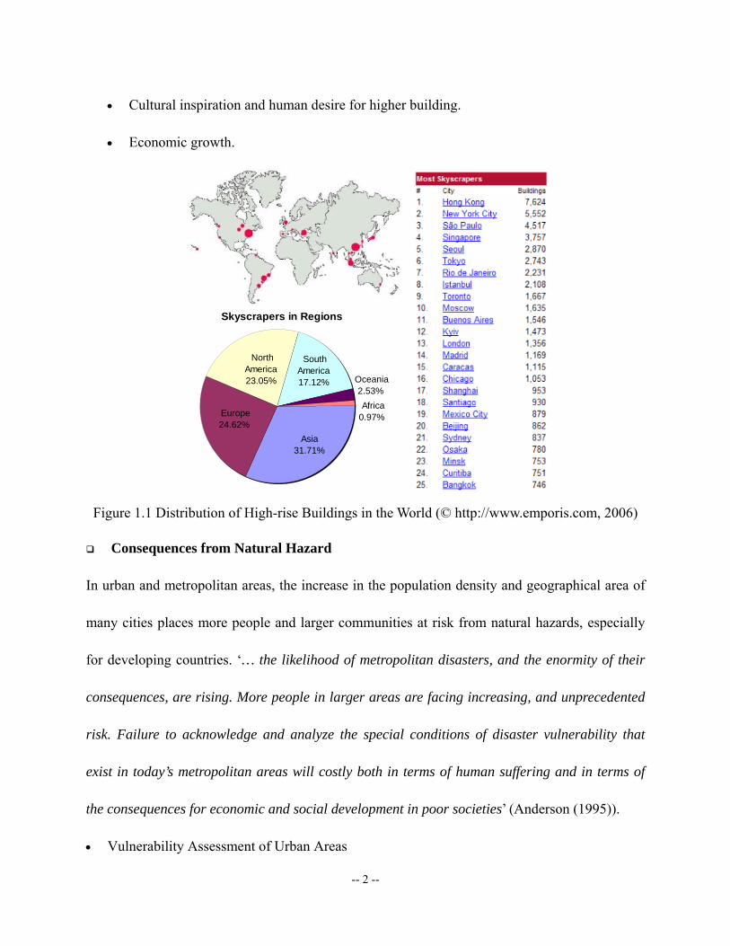
number and spreading in distribution around the world. Figure 1.1 shows the distribution of
high-rise buildings worldwide. The proliferation of high-rise buildings in urban area is speared
by several considerations amongst which:
• Pressure on land in urban areas and increasing demand for office and residential space
needs.
• Desire for aesthetics in urban areas and city skyline.
• Innovation in Structural Systems.
• Development of construction technology.
-- 2 --
• Cultural inspiration and human desire for higher building.
• Economic growth.
Skyscrapers in Regions
Europe24.62%
South America17.12%
Asia31.71%
North America23.05% Oceania
2.53% Africa0.97%
Figure 1.1 Distribution of High-rise Buildings in the World (© http://www.emporis.com, 2006)
Consequences from Natural Hazard
In urban and metropolitan areas, the increase in the population density and geographical area of
many cities places more people and larger communities at risk from natural hazards, especially
for developing countries. ‘… the likelihood of metropolitan disasters, and the enormity of their
consequences, are rising. More people in larger areas are facing increasing, and unprecedented
risk. Failure to acknowledge and analyze the special conditions of disaster vulnerability that
exist in today’s metropolitan areas will costly both in terms of human suffering and in terms of
the consequences for economic and social development in poor societies’ (Anderson (1995)).
• Vulnerability Assessment of Urban Areas

-- 3 --
Assessment of the potential severity of the consequences of a particular hazard involves the
assessment of vulnerability. Large cities exacerbate the human vulnerabilities because of the
difficulties of controlling and mitigating the hazard caused by potential disasters. Residential
vulnerability is fundamentally dependent upon the nature of the buildings and infrastructure
surrounding them. Among these, high-rise buildings, as residential, commercial, financial or
cultural centers, are most significant in the potential consequences from natural hazard events
since they usually represent concentrated economic and human assets.
• Fragility Assessment of RC High-rise Buildings
Vulnerability for structures, also referred to as fragility, is directly related to structural damage
extent and overall performance during or after the disaster. Damage has direct and indirect
consequences. For high-rise buildings, damage can cause significant losses in human life and
injuries due to structural collapse and fire. Indirect consequences may include the blockage of
transportation, inefficient casualty evacuation, diseases, and other longer-term national and
possibly international consequences. Therefore, to predict and mitigate the risk effectively,
fragility assessment of high-rise buildings is essential not only for new constructions but also for
the existing and largely non-seismically designed stock.
Reinforced concrete (RC) is now the principal structural material used in the construction of
high-rise structures. The tendency to use RC systems is expected to continue due to the
development of commercial high-strength concretes up to 170 MPa, the advent of admixtures
that can provide high fluidity without segregation and advances in construction techniques in
both pumping and formwork erection (Ali (2001)). The moldability of concrete is a major factor
-- 4 --
in creating exciting building forms with elegant aesthetic expression. Concrete is selected as a
primary structural material also because it is a naturally fireproof material and monolithic
concrete can absorb thermal movements, shrinkage and creep, and foundation movements.
Compared to steel, concrete tall buildings have larger masses and damping ratios that help in
minimizing perceptible motion. New structural systems including the composite option that are
popular now have allowed concrete buildings to reach new heights.
Due to the significance of wind forces on the lateral load demands in high-rise structures, the
effects of lateral loads from seismic action are often not considered in detail under different
earthquake scenarios. This can be quite inappropriate, because when assessing the seismic
performance of high-rise buildings it is important to consider that: (1) the wide frequency content
in real ground motions might excite both lower and higher modes and produce very complex
seismic demands; and (2) the imposed displacements in earthquakes may be very substantial
since the standard earthquake displacement spectrum peaks in the period of about 3-6 seconds.
This period range corresponds to the fundamental modes of many RC high-rise structures,
especially when responding in the inelastic range.
There is presently very limited information available to determine the seismic fragility of
high-rise buildings. For example, one of the most influential features of RC high-rise building
response is the response of RC walls. However, research on different configurations of complex
walls is not mature enough to enable the complete understanding of high-rise seismic behavior.
In current literature, only a few existing experimental data characterize both global response and
localized strain fields of complex walls.
-- 5 --
For the reasons above, there is the need for an improved understanding of the inelastic dynamic
response of RC high-rise structures subjected to realistic earthquake records representative of
near and far earthquakes. Moreover, motivated by the increasing interest in obtaining more
accurate assessments of earthquake losses, there is the need for deriving probabilistic fragility
relationships for high-rise structures.
1.2 Objectives
This research aims at deriving probabilistic assessment procedures for seismic vulnerability of
RC high-rise buildings and demonstrates the procedure through a reference application. The
study includes all the essentials included in the framework, such as seismic analysis of typical
building, uncertainty modeling of capacity and demand, definition of limit states and final
derivation of fragility functions. A comprehensive framework and its demonstration are sought,
in order to provide the tools needed for future studies that would cover most different types of
high-rise buildings for the purposes of assessing earthquake impact on large cities.
Since most RC high-rise buildings use complex wall systems as the main earthquake resisting
system, analytical modeling and corresponding experimental validations for structural walls is a
critical part of this research. The goal is to build accurate, reliable and efficient analytical tools
for structural walls and the whole building including wall-frame interaction effects.
1.3 Organization of the Report
The report documents completed studies of the essential areas discussed in the previous section,
-- 6 --
as well as a literature survey, proposed framework, case study, results, and discussion. Following
this introductory chapter, Chapter 2 is a general literature review of RC high-rise buildings and
fragility assessments. It includes basic configurations and information related to the structural
design of RC high-rise buildings, fragility assessment requirements, and the general framework
for deriving fragility relationships.
Chapter 3 describes the analytical structural modeling of a typical RC high-rise building. A
literature survey of RC materials, structural components and seismic analysis approaches is
briefly summarized. Then detailed modeling descriptions are given both at the material level for
concrete and reinforcement steel as well as at the structural component level for frames and walls.
Next, the two advanced Finite Element Analysis (FEA) software platforms employed in this
study are introduced and verifications are presented. The chapter highlights the importance of
developing a lumped-parameter-based model in the fragility assessment for a high-rise building.
The lumped-modeling process is illustrated in detail with the selected 54-story high-rise building,
and the chapter includes the proposed methodology, the derivation of a two-stage simplified
model using the Genetic Algorithm for parametric studies, and final lumped-model evaluations.
Chapter 4 defines new limit states for RC high-rise buildings. Based on the brief literature review,
a new qualitative definition is proposed for the limit states. Following this, the chapter discusses
the pushover analyses that were conducted to detect both global and local structural behaviors.
Then the newly developed multi-resolution distributed FEM analysis (MDFEA) method is
summarized, including the concept, model derivation and application for the analysis of real
structures. Finally, quantitative definitions of the new limit states are proposed.

-- 7 --
Chapter 5 presents a study of uncertainty modeling. After a brief literature survey of probabilistic
seismic demand and capacity, major sources of uncertainty, including ground motions and
materials, are investigated and discussed. The dominant uncertainty source was determined based
on the evaluation of random parameters and the effects on the numerical simulation for fragilities
are noted.
Chapter 6 describes the derivation of fragility relationships. This chapter starts with a literature
survey of existing fragility curves and then highlights the specific analytical fragility assessment
framework used for this study. Numerical simulations were conducted and are presented in the
chapter. Specific topics related to the numerical simulations including selecting and scaling
intensity measures, adopting effective duration concepts, fragility derivation through dynamic
response history analyses, and log-normal regression functions.
Chapter 7 summarizes the report. Conclusions are drawn about the process, proposed framework,
fragility results for RC high-rise buildings, and the research findings. Finally, future work is
proposed that will extend this research method to types of high-rise buildings besides the
reference structure.
-- 8 --
2. Seismic Fragility Assessment of RC High-rise Buildings
This chapter provides an overview of the forms of Reinforced Concrete (RC) High-rise buildings,
special considerations for the seismic performance and design of these structures, and an
introduction to methods for their fragility assessment.
2.1 RC High-rise Building Configuration and Design
As the height of RC concrete buildings increase, so due the complexity of structural forms and
the structural engineering design challenge. The design of tall buildings is particularly sensitive
to advancements in material science, construction techniques, methods of analysis, and wind
engineering. For example, concretes with compressive strength of up 24 ksi (165 MPa) are now
commercially available and advancements in mix design and chemical admixtures enable
concrete to be more easily and reliably placed. This has enabled reinforced concrete high-rise
buildings to become the material of choice in the design of world’s tallest buildings, with
full-height RC solutions being possible. The design of tall buildings is also very sensitive to the
imagination and aspirations of both designers and owners who in their desire to produce ever
taller signature structures take advantage of new materials, forms, techniques and innovative
approaches. This includes new structural systems such as the introduction of composite
construction to tall tubular buildings, first conceived and used by Fazlur Khan in the 1960s,
which paved the way for famous composite buildings including the Petronas Towers and Jin Mao
building in recent years.
-- 9 --
Due to the special features and forms of high-rise buildings, there has arisen the classification of
buildings according to both height and structural configuration. These classifications are
described in the next two subsections.
2.1.1 High-rise Building Definition
According to The Council of Tall Buildings and Urban Habitat, the description of ‘Tall building’,
equivalent to ‘High-rise building’ used herein, is: “A building whose height creates different
conditions in the design, construction, and use than those that exist in common buildings of a
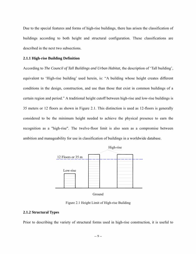
certain region and period.” A traditional height cutoff between high-rise and low-rise buildings is
35 meters or 12 floors as shown in Figure 2.1. This distinction is used as 12-floors is generally
considered to be the minimum height needed to achieve the physical presence to earn the
recognition as a "high-rise". The twelve-floor limit is also seen as a compromise between
ambition and manageability for use in classification of buildings in a worldwide database.
12 Floors or 35 m
Ground
Low-rise
High-rise
Figure 2.1 Height Limit of High-rise Building
2.1.2 Structural Types
Prior to describing the variety of structural forms used in high-rise construction, it is useful to
-- 10 --
first discuss the role taken by “shear” (or “structural”) walls. Khan and Sbarounis (1964)
introduced a novel design approach that took advantage of the interaction between rigid frames
and shear walls. A combination of the two structural components leads to a highly efficient
system, in which the shear wall (or a truss) resists the majority of the lateral loads in the lower
portion of the building, and the frame supports the majority of the lateral loads in the upper
portion of the building. The innovation of combining the frame with shear trusses or walls
allowed Khan to design economically competitive buildings up to 40 stories. This approach is
now extensively used in the design of 20- to 40-storey buildings either fully constructed in
concrete or composite with steel.
Another significant innovation in high-rises was proposed by Khan and Rankine (1980), who
proposed the idea of using a hollow thin-walled tube with punched holes to form the exterior of
buildings. By reducing the spacing of exterior columns, the entire system of beams and columns
lying on the external perimeter of a building can be made to act as a perforated or framed tube.
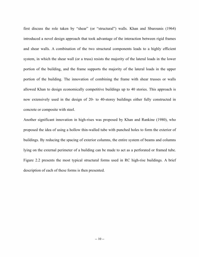
Figure 2.2 presents the most typical structural forms used in RC high-rise buildings. A brief
description of each of these forms is then presented.
-- 11 --
Figure 2.2 Concrete Systems Suitable for Buildings with Different Number of Stories (after Ali (2001))
Moment Resisting Frame Systems (MRF)
Moment-resisting frames are structures with traditional beam-column frames that carry the
gravity loads that are imposed on the floor system. The floors also function as horizontal
diaphragm elements that transfer lateral forces to the girders and columns. While a MRF may be
designed to resist the lateral load from wind or seismic actions, it is more common to provide
another lateral load resisting system.
Braced Frame (BF), Shear Wall Systems (SW)
To increase the lateral load resisting capacity and reduce relative translations, diagonal braces are
frequently added to MRF. These braces enable the downward flow of lateral loads by axial
tension and compression in these braces and membrane actions in floors without significant
flexural demands being placed on the MRF. Rather than diagonal braces, it is also common to us
“shear” (or “structural”) walls. The lateral stiffness of these walls is typically so much greater
than that of the MRF in lower high-rise buildings that the lateral load is considered to be entirely
-- 12 --
resisted by the walls. Structural walls were first used in 1940s. An additional benefit for the use
of RC walls is that their significant mass dampens a building vibration.
Core and Outrigger Systems (COS)
A combined system called a shear wall-frame interaction system, as first seriously studied by
Fazlur Khan, was a milestone in the development of taller concrete buildings. In this system, a
central core or dispersed shear walls interact with the remaining beam-column or slab-column
framing and in which lateral loads are transmitted by floor diaphragms. The outer part is referred
to as the “Outrigger System”. As previously described, the interaction of these two systems
enabled a more effective use of both frames and walls.
Tubular Systems (TS)
A tubular structure acts as a stiffened three-dimensional framework where the entire building
works to resist overturning moments. Tubes can be composed of shear walls and frames that act
as a single unit. The main feature of a tube is closely spaced exterior columns connected by deep
spandrels that form a spatial skeleton and are advantageous for resisting lateral loads in a
three-dimensional structural space. The primary types of tubular structures are Framed or Braced
Tubes, Trussed Tubes, Tube-in-Tube, and Bundled Tubes.
Tubular core walls are designed to carry the full lateral load or to interact with frames. This gives
the building a tube-in-tube appearance although it was designed using the shear wall-frame
interaction principle. A tube-in-tube is a system with framed tube that has an external and
internal shear wall core which act together to resist the lateral loads. Bundled tubes are used in
very large structures as a way of decreasing the surface exposed to wind. Multiple tubes share
-- 13 --
internal and adjoining columns depending on their adjacencies.
Hybrid Systems (HS)
Through advancements in material properties, construction techniques and structural knowledge,
more complex but efficient structural form have emerged. They are typically some combination
of tube and outrigger system, use either concrete or steel composite systems, and are thereby
generally referred to as hybrid systems. One example is the structural frames for the 1,483 ft
(452 m) tall Petronas Towers, in Kuala Lumpur, Malaysia, that used columns, core walls, and
ring beams made of high-strength concrete but then steel floor beams and decking for faster
construction and future adaptation. The core and frame act together to provide the needed lateral
stiffness for these very tall towers. Another example of a hybrid system is the 1,380 ft (421 m)
high Jin Mao building that was completed in 1999 in Shanghai, China. This structure has a
hybrid system with a number of steel outrigger trusses tying the building's concrete core to its
exterior composite mega-columns.
2.2 Seismic Design and Performance of RC High-rise Systems
According to Laogan and Elnashai (1999), the characteristics of the previously-described
structural forms determine performance during earthquake strikes. Hence a structure’s suitability
for seismic applications depends on this performance. Table 2.1 presents the general
characteristics of each of these forms and their suitability for use in seismic regions.

-- 14 --
Table 2.1 Efficiency of RC High-rise Systems for Seismic Applications
(after Laogan and Elnashai (1999))
Suitability
System Type Stiffness Strength Ductility Max number of stories
Seismic application
Moment Resisting Frame L H H 15-20 ��
Braced Frame H H L-M 20-30 �
Structural Wall H H L-M 25-30 �
Hybrid Frame H H M-H 30-40 ��
Core and Outrigger System H H L-M 50-60 �
Framed Tube System H H M-H 60-70 ��
Tube-in-Tube System H H M-H 70-80 ��
Trussed Tube System H H M-H 80-100 ��
Bundled Tube System H H M-H 120-150 ��
Notes: H = High; M = Moderate; L = Low; � = Suitable; �� = Very Suitable.
Due to the economic necessity of incorporating advancements in materials, construction
techniques, and analysis methods, the structural design of high-rise buildings is inherently
innovative. High-rise buildings typically must be designed to resist significant lateral loads
imposed by wind effects from typhoons or hurricanes or due to inertial forces caused by seismic
strikes. The overall structural response under wind or seismic loads becomes the controlling
factor in most designs. Since the first publication of the Uniform Building Code (UBC) in 1926,
provisions for seismic design have been under continuous development and are evolving from
their empirical origins (Taranath (2005)). Changes to the provisions are based on improved

-- 15 --
understanding of structural behavior as well as advancements in numerical models and
computational capabilities.
Due to for the difficulty of precisely evaluating the dynamic response of high-rise structures
through laboratory experiments or non-linear analysis, much of our understanding of the seismic
behavior of tall structures comes from observations during seismic events. The poor response of
many structures during the Northridge (1994) and Kobe (1995) earthquakes inspired a
reexamination of structural design methods. For RC high-rise buildings, the limitations of
traditional strength-based design were recognized, and performance-based as well as
consequence-based evaluation approaches have emerged.
Two building codes have been developed and maintained for seismic design in the United States.
The International Building Code (IBC) was developed by the International Code Council (ICC),
and the second building code is the National Fire Protection Agency (NFPA) 5000 Code. The
seismic design provisions within both codes are consistent with the National Earthquake Hazard
Reduction Program (NEHRP) provisions. In addition, both codes incorporate major national
standards as references, including the ACI Building Code Requirements for Structural Concrete
(ACI-318) and the ASCE Minimum Design Loads for Buildings and Other Structures (ASCE 7)
provisions for seismic loads. To ensure acceptable performance of high-rise RC structures in
seismic regions, dynamic analyses and the use of seismic design principles need to be employed
at all stages in design.
-- 16 --
2.3 Requirements for Fragility Assessment
For hazard mitigation and risk analysis for populations of RC high-rise buildings, it is needed to
fully assess and synthesis the potential damage to such structures. A first key step is to define
acceptable damage and establish performance criteria for different structure forms under
different natural hazards. This requires the use of fragility assessment methods, which allow the
prediction of the probability of occurrence of different damage states and under different natural
hazards. This study focuses on earthquake hazards.
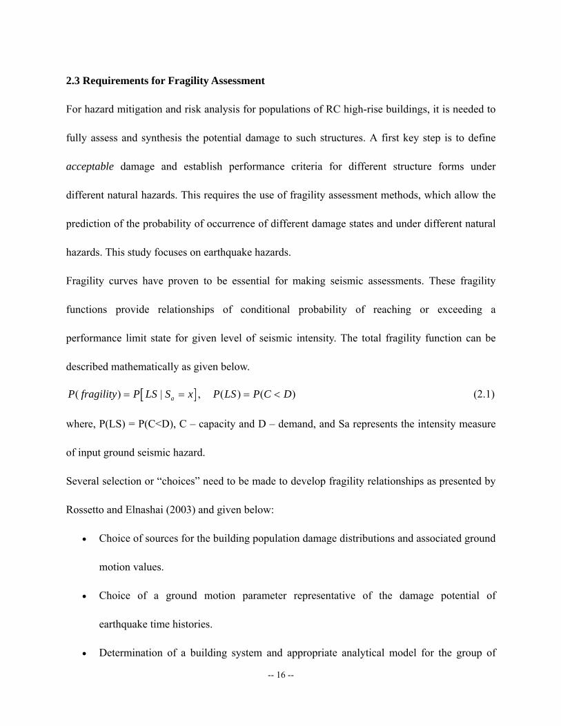
Fragility curves have proven to be essential for making seismic assessments. These fragility
functions provide relationships of conditional probability of reaching or exceeding a
performance limit state for given level of seismic intensity. The total fragility function can be
described mathematically as given below.
[ ]( ) | , ( ) ( )aP fragility P LS S x P LS P C D= = = < (2.1)
where, P(LS) = P(C<D), C – capacity and D – demand, and Sa represents the intensity measure
of input ground seismic hazard.
Several selection or “choices” need to be made to develop fragility relationships as presented by
Rossetto and Elnashai (2003) and given below:
• Choice of sources for the building population damage distributions and associated ground
motion values.
• Choice of a ground motion parameter representative of the damage potential of
earthquake time histories.
• Determination of a building system and appropriate analytical model for the group of
-- 17 --
damage statistics for buildings with similar dynamic response characteristics.
• Selection of damage scales and the definition of limit states for the assessment of
building performance.
• Choice of a structural response parameter for estimation of global building damage, and
determination of its value at the thresholds of the chosen limit states.
• Determination of a procedure for the interpretation of the building damage statistics in
terms of the chosen damage scales.
• Choice of a methodology for the damage data combination and confidence bound
estimation.
• Selection of shape functions for fragility curves and of regression procedures.
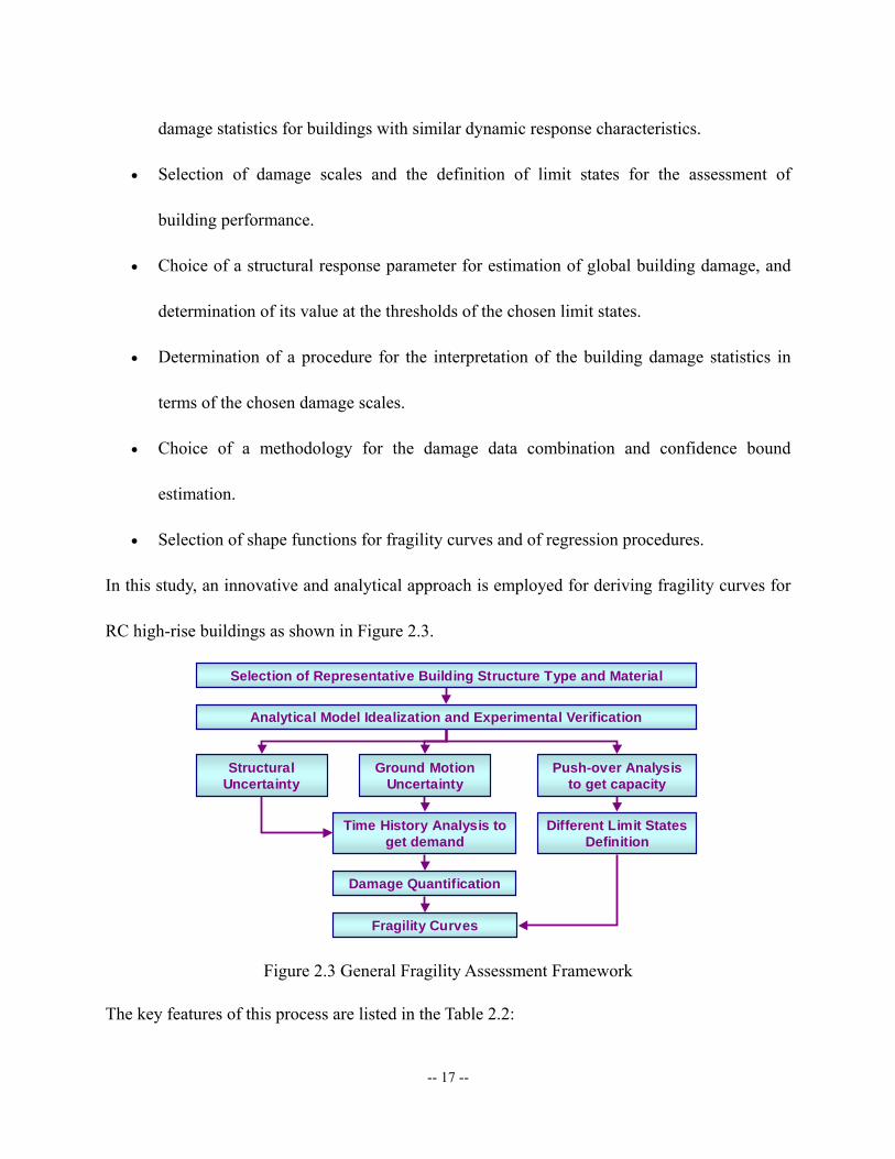
In this study, an innovative and analytical approach is employed for deriving fragility curves for
RC high-rise buildings as shown in Figure 2.3.
Selection of Representative Building Structure Type and Material
Analytical Model Idealization and Experimental Verification
Push-over Analysis to get capacity
Ground Motion Uncertainty
Structural Uncertainty
Different Limit States Definition
Time History Analysis to get demand
Fragility Curves
Damage Quantification
Figure 2.3 General Fragility Assessment Framework
The key features of this process are listed in the Table 2.2:
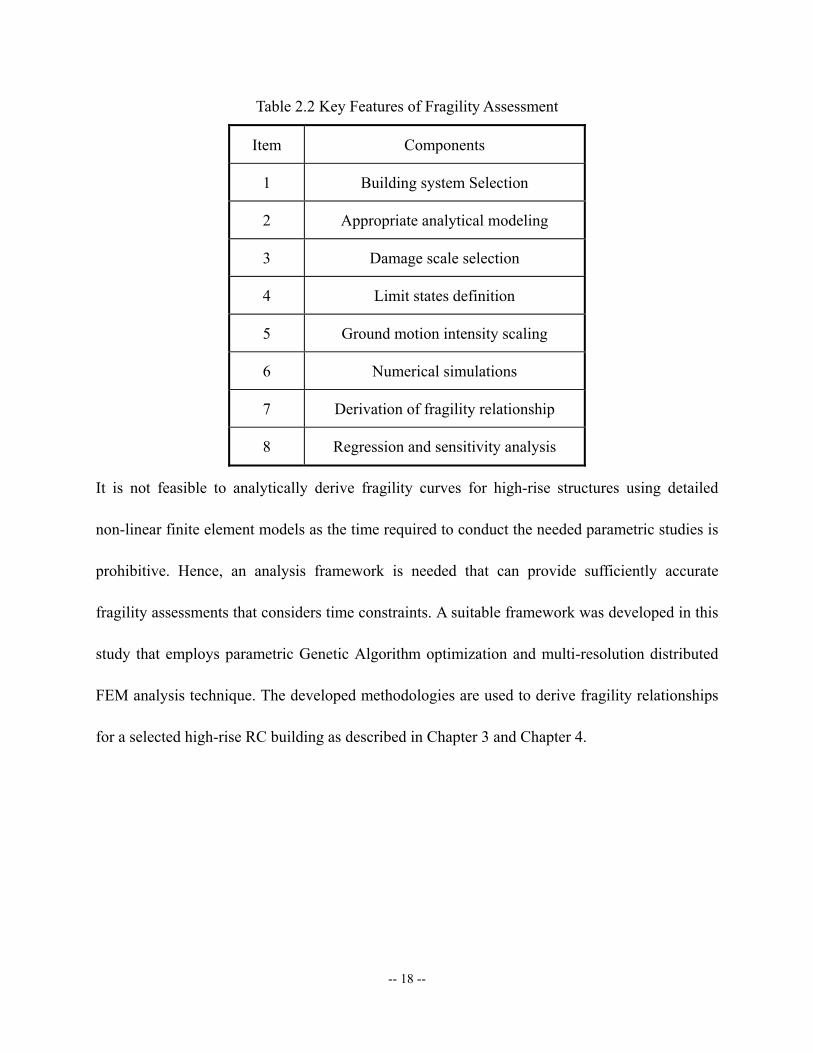
-- 18 --
Table 2.2 Key Features of Fragility Assessment
Item Components
1 Building system Selection
2 Appropriate analytical modeling
3 Damage scale selection
4 Limit states definition
5 Ground motion intensity scaling
6 Numerical simulations
7 Derivation of fragility relationship
8 Regression and sensitivity analysis
It is not feasible to analytically derive fragility curves for high-rise structures using detailed
non-linear finite element models as the time required to conduct the needed parametric studies is
prohibitive. Hence, an analysis framework is needed that can provide sufficiently accurate
fragility assessments that considers time constraints. A suitable framework was developed in this
study that employs parametric Genetic Algorithm optimization and multi-resolution distributed
FEM analysis technique. The developed methodologies are used to derive fragility relationships
for a selected high-rise RC building as described in Chapter 3 and Chapter 4.

-- 19 --
3. Analytical Structural Modeling
3.1 Literature Survey
The analysis methods for RC high-rise buildings have special requirements different from
low-to-middle rise buildings, especially for the typical structural system that consists of slender
members in frames and more RC stocky structural walls. The complexities of concrete properties,
wall-frame interaction and three-dimensional effects need to be accounted for in structural
modeling.
The development of an analytical model to predict the response of RC high-rise structures to
seismic actions is complicated by the different types of structural elements and the inherently
inelastic and non-linear and degrading behavior of reinforced concrete. The behavior of the
beams and columns can usually be adequately captured by fiber-based or multi-layer beam
elements in which only a strength check is made for shear. For walls, either continuum analysis
is required or the effects of shear must be handled separately. While the lateral response of a RC
high-rise structure to seismic actions is typically dominated by the response of the wall, it is
essential to consider the contribution of the frame and the frame-wall interactions to obtain
sufficiently accurate results from the dynamic response-history analyses.
3.1.1 Material Properties
Many researchers have developed constitutive relationships for concrete based on a variety of
experimental tests. Shah and Slate (1968) analyzed the micro-mechanism of the idealization of
stresses around a single aggregate particle to understand the flow and bond between paste and
-- 20 --
aggregates. Darwin and Slate (1970) quantified and compared the effects considering different
aggregate types. Ahmad and Shah (1985) and Mendis (2003) obtained the stress-strain curves for
concretes for different concrete strengths ranging from 4.0~12.0 ksi. Based on a lot of
investigations of test data, many concrete constitutive models have been proposed, for the
compressive response of concrete, including the commonly used model by Popovics (1973) and
Hognestad Parabolic Model for concrete behavior under uniaxial loading, and nonlinear biaxial
stress-strain laws by Kupfer et al. (1969), Kupfer and Gerstle (1973) and Darwin and Pecknold
(1977), etc. Other response characteristics have been studied including the modulus of elasticity,
Poisson’s Ratio, confining effects, cyclic loading responses, and so on. In recent years, high
strength concrete (HSC) or high performance concrete (HPC) has become popular for application
in high-rise buildings as it increases the height potential for RC construction, reduces weight, and
increases available floor areas. ACI Committee 363 has documented the different behaviors of
HSC as to their stress-strain relationships, failure modes and time-dependent behavior (ACI
(1997)).
Typical stress-strain curves for reinforcing steel bars were obtained from many tests of bars
loaded monotonically in tension. For all practical purposes steel exhibits the same stress-strain
response in compression as in tension and symmetric cyclic loading responses can be reasonably
assumed. Bi-linear or tri-linear (with one flat yield plateau) constitutive relationships have
proven to be accurate enough to meet the need of analysis, especially at the structural level (Ngo
and Scordelis (1967); Bashur and Darwin (1978)).
-- 21 --
3.1.2 Structural Components
No matter what type and size of RC structure is under investigation the finite element method
(FEM) is the most accurate and reliable analytical technique for assessing the demands on
structure components in both 2D and 3D domains. The earliest application to the analysis of RC
structures was by Ngo and Scordelis (1967). Scordelis et al. (1974) used the same approach to
study the behavior of beams in shear. Nilson (1972) introduced nonlinear material properties for
concrete and steel and a nonlinear bond-slip relationship into the analysis. Nayak and
Zienkiewicz (1972) conducted two-dimensional stress studies that include the tensile cracking
and the elasto-plastic behavior of concrete in compression using an initial stress approach. For
the analysis of RC beams with material and geometric nonlinearities Rajagopal (1976) developed
a layered rectangular plate element with axial and bending stiffness treating concrete as an
orthotropic material. RC frame problems have also been treated by many other investigators
(Bashur and Darwin (1978); Adeghe and Collins (1986); Bergmann and Pantazopoulou (1988))
using similar methods. At the same time the damage and crack simulation have also been studied
and generated some representative models, such as the concept of a smeared crack model
introduced by Rashid (1968) and revised or extended by researches like Meyer and Okamura
(1985).
According to the buildings categories described in section 2.1.2, typical RC high-rise structures
will consist of the following components:
Structural Wall
Structural walls serve as the major lateral resisting component, providing much larger stiffness or
-- 22 --
capacity in strong directions than other members. The relatively larger width to thickness ratio of
walls makes their shear stiffness and strength significantly larger than normal beams and
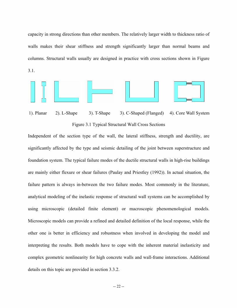
columns. Structural walls usually are designed in practice with cross sections shown in Figure
3.1.
1). Planar 2). L-Shape 3). T-Shape 3). C-Shaped (Flanged) 4). Core Wall System
Figure 3.1 Typical Structural Wall Cross Sections
Independent of the section type of the wall, the lateral stiffness, strength and ductility, are
significantly affected by the type and seismic detailing of the joint between superstructure and
foundation system. The typical failure modes of the ductile structural walls in high-rise buildings
are mainly either flexure or shear failures (Paulay and Priestley (1992)). In actual situation, the
failure pattern is always in-between the two failure modes. Most commonly in the literature,
analytical modeling of the inelastic response of structural wall systems can be accomplished by
using microscopic (detailed finite element) or macroscopic phenomenological models.
Microscopic models can provide a refined and detailed definition of the local response, while the
other one is better in efficiency and robustness when involved in developing the model and
interpreting the results. Both models have to cope with the inherent material inelasticity and
complex geometric nonlinearity for high concrete walls and wall-frame interactions. Additional
details on this topic are provided in section 3.3.2.
-- 23 --
Beam-Column Frame
Frame members primarily serve to carry the majority of gravity loads in a building, but also
serve as part of lateral resisting systems. The beams and columns have varieties of cross section
types including rectangular, T–shape and I–Shape. In FEM analysis, it is very straightforward to
use beam element connected by rigid joints to form the frame. Bernoulli-Euler beam theory and
Timoshenko beam theory (Hjelmstad (2005)) if considering shear effects for deep beam, are
widely used and have been implemented into most computer-based frame analysis packages. In
order to model inelastic behavior, fiber models are employed as discussed in section 3.3.1.
Floor System
There are a large variety of floor systems, used in high-rise construction. The selected system
must consider the building functionalities, space requirements, construction techniques,
reduction of dead loads and cost-effectiveness. Floor system in high-rise buildings functions not
only provides gravity load resistance, but also provides constraints between frames, walls, and
core and outrigger systems, with great contribution to spatial components interactions. Therefore,
in analytical modeling, floor system will be simulated according to the purpose of analysis,
which indicates that, if spatial load path and stress strain fields are desired, then detailed
modeling for slabs and related beams are necessary in FEA, otherwise simplification into
equivalent beam elements or even sets of springs or rigid bars (the part within wall or column
regions) are sufficient to obtain overall building response especially in designated directions.
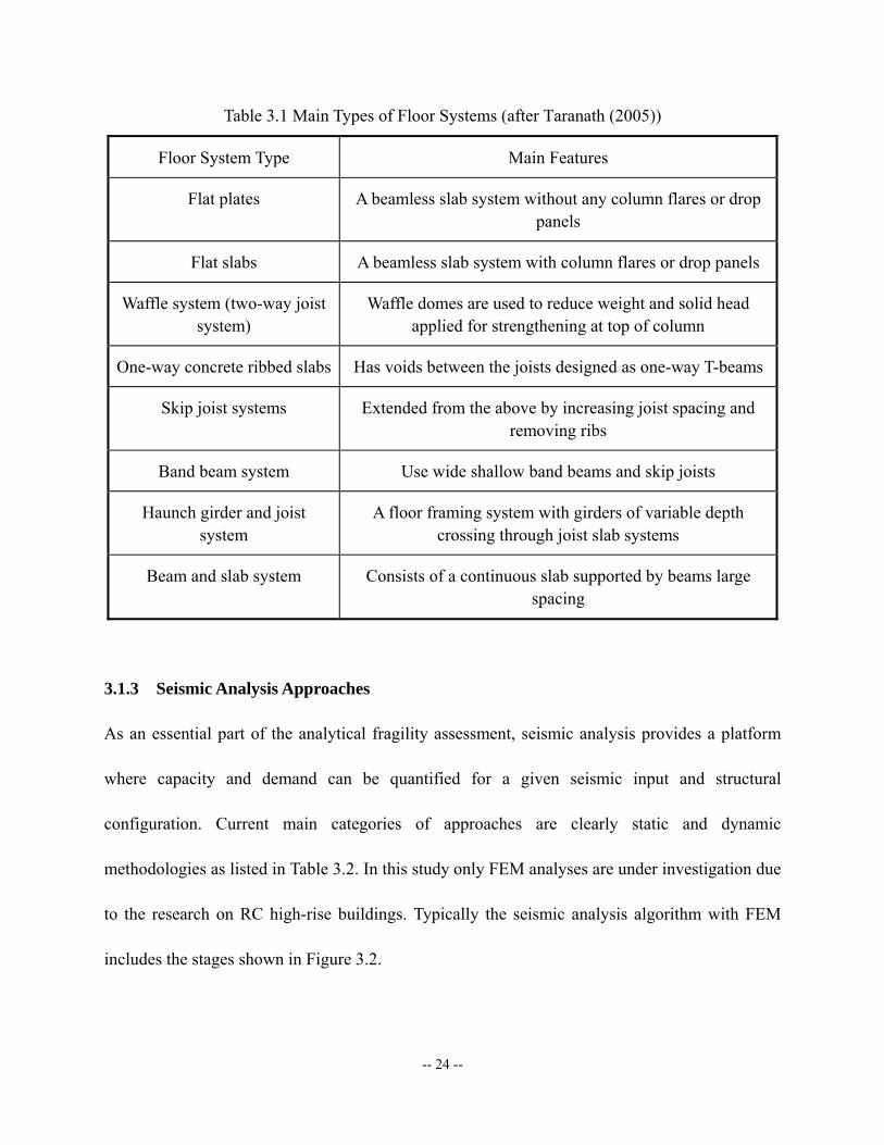
Main types of floor systems are listed in Table 3.1 after Taranath (2005).
-- 24 --
Table 3.1 Main Types of Floor Systems (after Taranath (2005))
Floor System Type Main Features
Flat plates A beamless slab system without any column flares or drop panels
Flat slabs A beamless slab system with column flares or drop panels
Waffle system (two-way joist system)
Waffle domes are used to reduce weight and solid head applied for strengthening at top of column
One-way concrete ribbed slabs Has voids between the joists designed as one-way T-beams
Skip joist systems Extended from the above by increasing joist spacing and removing ribs
Band beam system Use wide shallow band beams and skip joists
Haunch girder and joist system
A floor framing system with girders of variable depth crossing through joist slab systems
Beam and slab system Consists of a continuous slab supported by beams large spacing
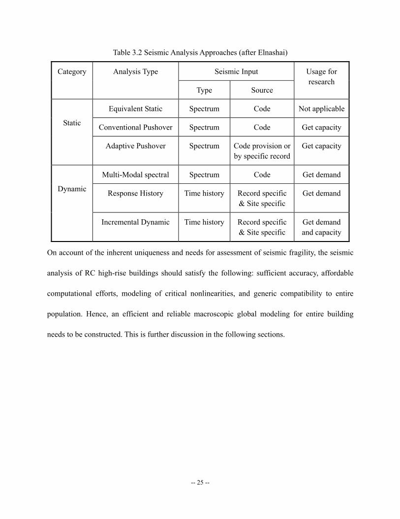
3.1.3 Seismic Analysis Approaches
As an essential part of the analytical fragility assessment, seismic analysis provides a platform
where capacity and demand can be quantified for a given seismic input and structural
configuration. Current main categories of approaches are clearly static and dynamic
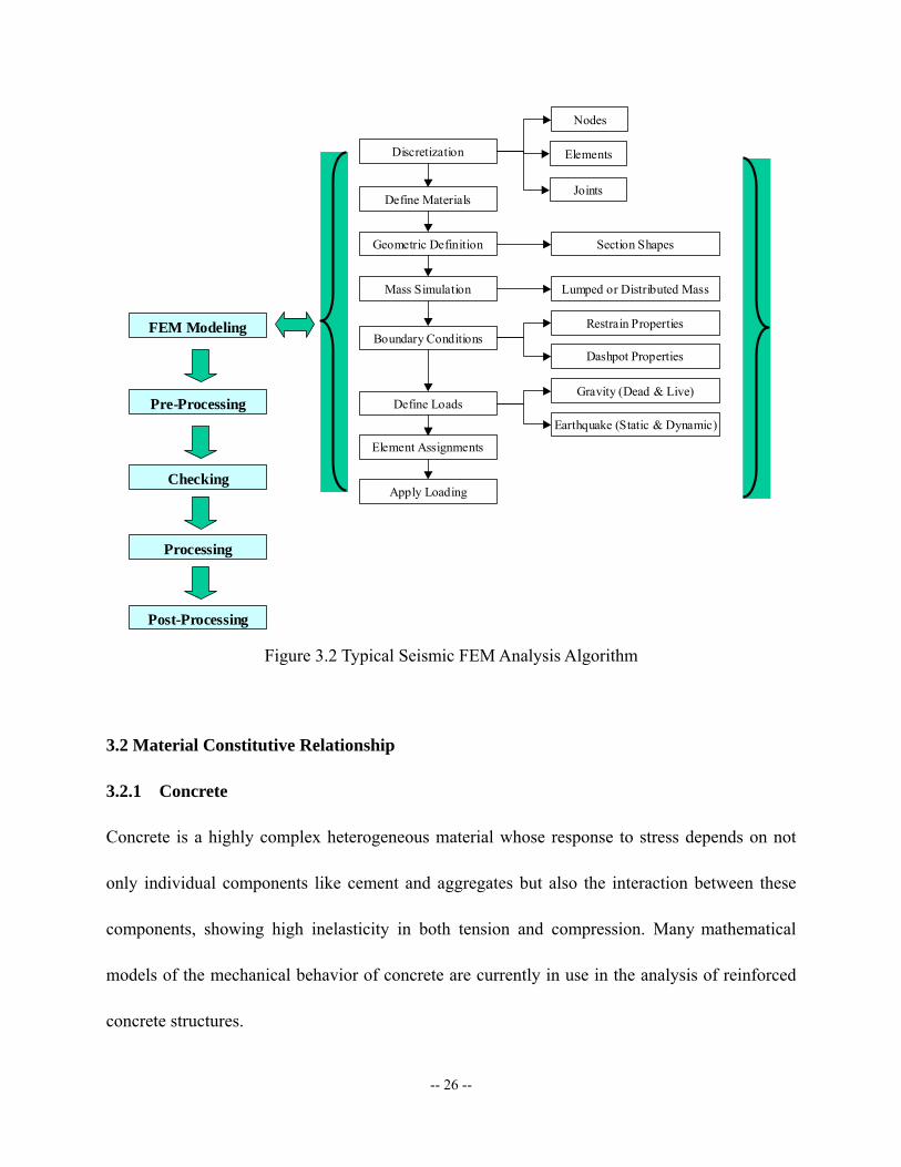
methodologies as listed in Table 3.2. In this study only FEM analyses are under investigation due
to the research on RC high-rise buildings. Typically the seismic analysis algorithm with FEM
includes the stages shown in Figure 3.2.
-- 25 --
Table 3.2 Seismic Analysis Approaches (after Elnashai)
Seismic Input Category Analysis Type
Type Source
Usage for research
Equivalent Static Spectrum Code Not applicable
Conventional Pushover Spectrum Code Get capacity
Static
Adaptive Pushover Spectrum Code provision or by specific record
Get capacity
Multi-Modal spectral Spectrum Code Get demand
Response History Time history Record specific & Site specific
Get demand
Dynamic
Incremental Dynamic Time history Record specific & Site specific
Get demand and capacity
On account of the inherent uniqueness and needs for assessment of seismic fragility, the seismic
analysis of RC high-rise buildings should satisfy the following: sufficient accuracy, affordable
computational efforts, modeling of critical nonlinearities, and generic compatibility to entire
population. Hence, an efficient and reliable macroscopic global modeling for entire building
needs to be constructed. This is further discussion in the following sections.
-- 26 --
Discretization
Define Materials
Define Loads
Element Assignments
Apply Loading
Nodes
Elements
Joints
Gravity (Dead & Live)
Earthquake (Static & Dynamic)
FEM Modeling
Pre-Processing
Checking
Processing
Post-Processing
Mass Simulation
Restrain Properties
Dashpot PropertiesBoundary Conditions
Geometric Definition Section Shapes
Lumped or Distributed Mass
Figure 3.2 Typical Seismic FEM Analysis Algorithm
3.2 Material Constitutive Relationship
3.2.1 Concrete
Concrete is a highly complex heterogeneous material whose response to stress depends on not
only individual components like cement and aggregates but also the interaction between these
components, showing high inelasticity in both tension and compression. Many mathematical
models of the mechanical behavior of concrete are currently in use in the analysis of reinforced
concrete structures.
-- 27 --
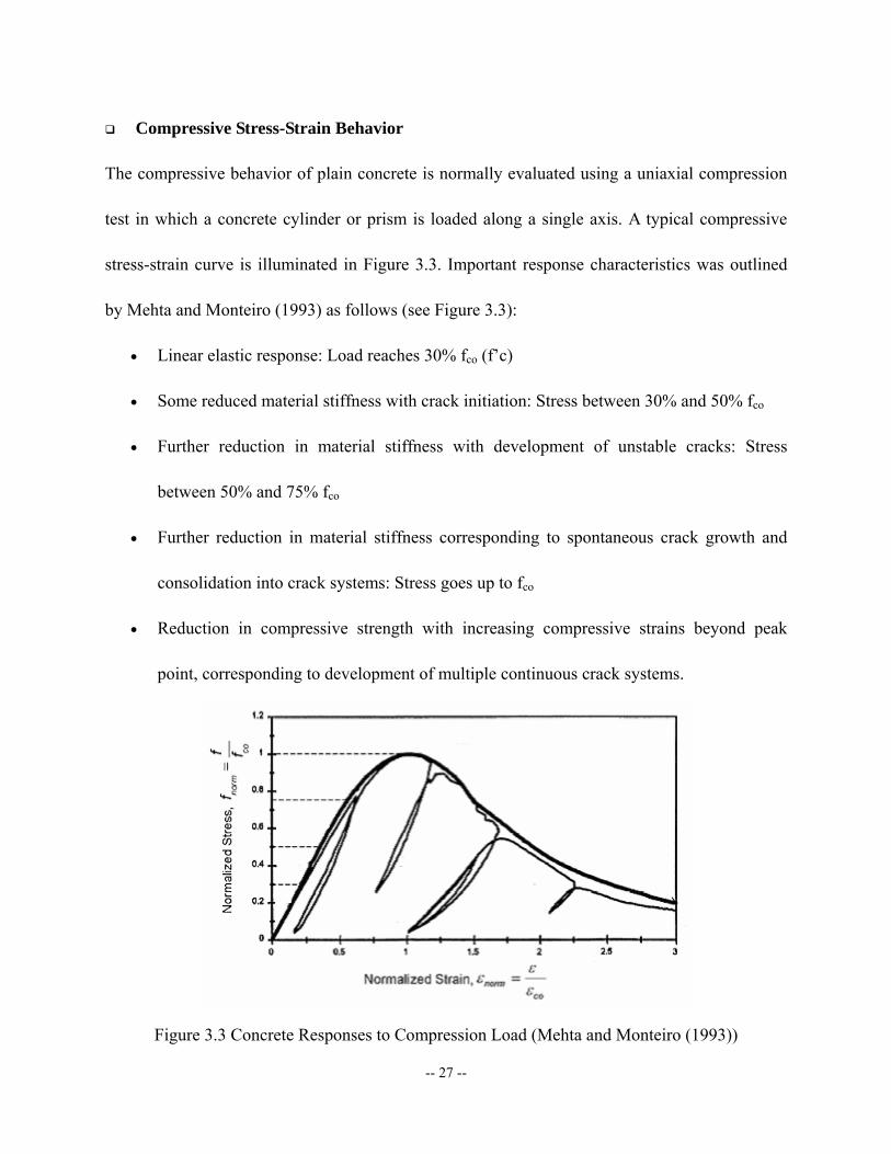
Compressive Stress-Strain Behavior
The compressive behavior of plain concrete is normally evaluated using a uniaxial compression
test in which a concrete cylinder or prism is loaded along a single axis. A typical compressive
stress-strain curve is illuminated in Figure 3.3. Important response characteristics was outlined
by Mehta and Monteiro (1993) as follows (see Figure 3.3):
• Linear elastic response: Load reaches 30% fco (f’c)
• Some reduced material stiffness with crack initiation: Stress between 30% and 50% fco
• Further reduction in material stiffness with development of unstable cracks: Stress
between 50% and 75% fco
• Further reduction in material stiffness corresponding to spontaneous crack growth and
consolidation into crack systems: Stress goes up to fco
• Reduction in compressive strength with increasing compressive strains beyond peak
point, corresponding to development of multiple continuous crack systems.
Figure 3.3 Concrete Responses to Compression Load (Mehta and Monteiro (1993))
-- 28 --
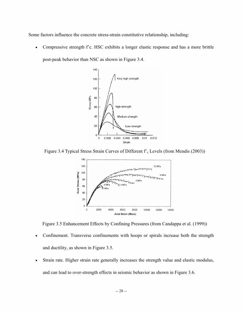
Some factors influence the concrete stress-strain constitutive relationship, including:
• Compressive strength f’c. HSC exhibits a longer elastic response and has a more brittle
post-peak behavior than NSC as shown in Figure 3.4.
Figure 3.4 Typical Stress Strain Curves of Different f’c Levels (from Mendis (2003))
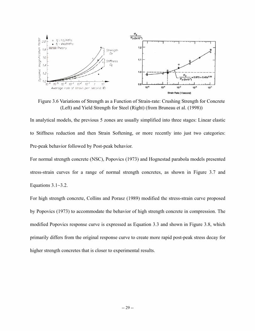
Figure 3.5 Enhancement Effects by Confining Pressures (from Candappa et al. (1999))
• Confinement. Transverse confinements with hoops or spirals increase both the strength
and ductility, as shown in Figure 3.5.
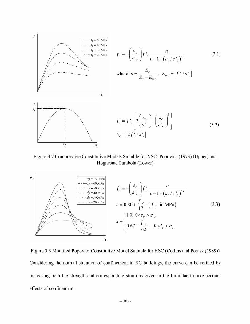
• Strain rate. Higher strain rate generally increases the strength value and elastic modulus,
and can lead to over-strength effects in seismic behavior as shown in Figure 3.6.
-- 29 --
Figure 3.6 Variations of Strength as a Function of Strain-rate: Crushing Strength for Concrete (Left) and Yield Strength for Steel (Right) (from Bruneau et al. (1998))
In analytical models, the previous 5 zones are usually simplified into three stages: Linear elastic
to Stiffness reduction and then Strain Softening, or more recently into just two categories:
Pre-peak behavior followed by Post-peak behavior.
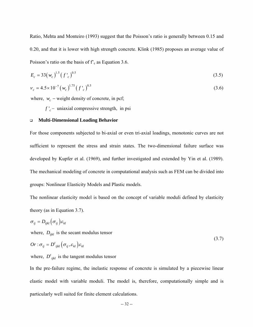
For normal strength concrete (NSC), Popovics (1973) and Hognestad parabola models presented
stress-strain curves for a range of normal strength concretes, as shown in Figure 3.7 and
Equations 3.1~3.2.
For high strength concrete, Collins and Porasz (1989) modified the stress-strain curve proposed
by Popovics (1973) to accommodate the behavior of high strength concrete in compression. The
modified Popovics response curve is expressed as Equation 3.3 and shown in Figure 3.8, which
primarily differs from the original response curve to create more rapid post-peak stress decay for
higher strength concretes that is closer to experimental results.
-- 30 --
( )'
' 1 / 'c
c c nc c c
nf fn
εε ε ε
⎛ ⎞= −⎜ ⎟
− +⎝ ⎠ (3.1)
secsec
where: , ' / 'cc c
c
En E f
E Eε= =
−
2
' 2' '
2 ' / '
c cc c
c c
c c c
f f
E f
ε εε ε
ε
⎡ ⎤⎛ ⎞ ⎛ ⎞⎢ ⎥= −⎜ ⎟ ⎜ ⎟⎢ ⎥⎝ ⎠ ⎝ ⎠⎣ ⎦
=
(3.2)
Figure 3.7 Compressive Constitutive Models Suitable for NSC: Popovics (1973) (Upper) and Hognestad Parabola (Lower)
( )
( )
'' 1 / '
'0.80 , ' in MPa
171.0, 0> '
'0.67 , 0> '
62
cc c nk
c c c
cc
c c
cc c
nf fn
fn f
k f
εε ε ε
ε ε
ε ε
⎛ ⎞= −⎜ ⎟
− +⎝ ⎠
= +
>⎧⎪= ⎨
+ >⎪⎩
(3.3)
Figure 3.8 Modified Popovics Constitutive Model Suitable for HSC (Collins and Porasz (1989))
Considering the normal situation of confinement in RC buildings, the curve can be refined by
increasing both the strength and corresponding strain as given in the formulae to take account
effects of confinement.

-- 31 --
Tensile Stress-Strain Behavior
In tension, concrete is predominantly brittle and its response can be differentiated into uncracked
and cracked response. The practical parameter is cracking strength fcr, which is associated with
factors such as specimen size, compressive strength, and the stress states. Some tensile stress
strain relationships have been proposed such as those by Vecchio and Collins (1982) Model and
its modification as Collins-Mitchell (1987) Model, shown as following Figure 3.9 and Equation
3.4.
Figure 3.9 Vecchio and Collins-Mitchell Tension Stiffening Response Models
, > >0
, > >0, (Vecchio 1982)1 200
, > >0, (Collins-Mitchell 1987)1 500
c crcr c
cr
crc c cr
c
crc cr
c
f
ff
f
εε ε
ε
ε εε
ε εε
⎧⎪⎪⎪⎪= ⎨
+⎪⎪⎪⎪ +⎩
(3.4)
Elastic Modulus and Poisson’s Ratio
The modulus of elasticity and also the strain corresponding to the peak stress increase with
increasing compressive strength, see Equation 3.5 according to ACI 1992. For the Poisson’s
-- 32 --
Ratio, Mehta and Monteiro (1993) suggest that the Poisson’s ratio is generally between 0.15 and
0.20, and that it is lower with high strength concrete. Klink (1985) proposes an average value of
Poisson’s ratio on the basis of f’c as Equation 3.6.
( ) ( )1.5 0.533 'c c cE w f= (3.5)
( ) ( )1.75 0.574.5 10 'c c cw fν −= × (3.6)
where, weight density of concrete, in pcf;
' uniaxial compressive strength, in psi
c
c
w
f
−
−
Multi-Dimensional Loading Behavior
For those components subjected to bi-axial or even tri-axial loadings, monotonic curves are not
sufficient to represent the stress and strain states. The two-dimensional failure surface was
developed by Kupfer et al. (1969), and further investigated and extended by Yin et al. (1989).
The mechanical modeling of concrete in computational analysis such as FEM can be divided into
groups: Nonlinear Elasticity Models and Plastic models.
The nonlinear elasticity model is based on the concept of variable moduli defined by elasticity
theory (as in Equation 3.7).
( )
( )
where, is the secant modulus tensor
: ,
where, is the tangent modulus tensor
ij ijkl ij kl
ijkl
tij ijkl ij kl kl
tijkl
D
D
Or D
D
σ σ ε
σ σ ε ε
=
= (3.7)
In the pre-failure regime, the inelastic response of concrete is simulated by a piecewise linear
elastic model with variable moduli. The model is, therefore, computationally simple and is
particularly well suited for finite element calculations.
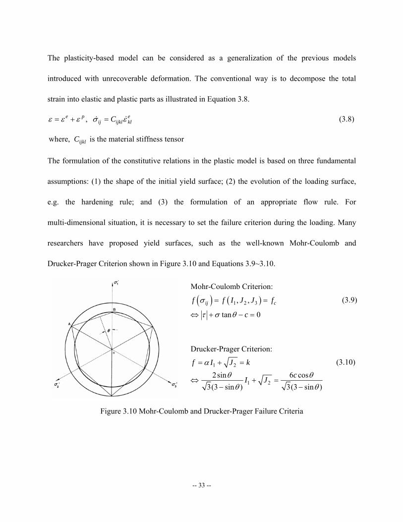
-- 33 --
The plasticity-based model can be considered as a generalization of the previous models
introduced with unrecoverable deformation. The conventional way is to decompose the total
strain into elastic and plastic parts as illustrated in Equation 3.8.
, e p eij ijkl klCε ε ε σ ε= + = && (3.8)
where, is the material stiffness tensorijklC
The formulation of the constitutive relations in the plastic model is based on three fundamental
assumptions: (1) the shape of the initial yield surface; (2) the evolution of the loading surface,
e.g. the hardening rule; and (3) the formulation of an appropriate flow rule. For
multi-dimensional situation, it is necessary to set the failure criterion during the loading. Many
researchers have proposed yield surfaces, such as the well-known Mohr-Coulomb and
Drucker-Prager Criterion shown in Figure 3.10 and Equations 3.9~3.10.
( ) ( )1 2 3
Mohr-Coulomb Criterion:
, ,
tan 0ij cf f I J J f
c
σ
τ σ θ
= =
⇔ + − =
(3.9)
1 2
1 2
Drucker-Prager Criterion:
2sin 6 cos3(3 sin ) 3(3 sin )
f I J kcI J
αθ θθ θ
= + =
⇔ + =− −
(3.10)
Figure 3.10 Mohr-Coulomb and Drucker-Prager Failure Criteria
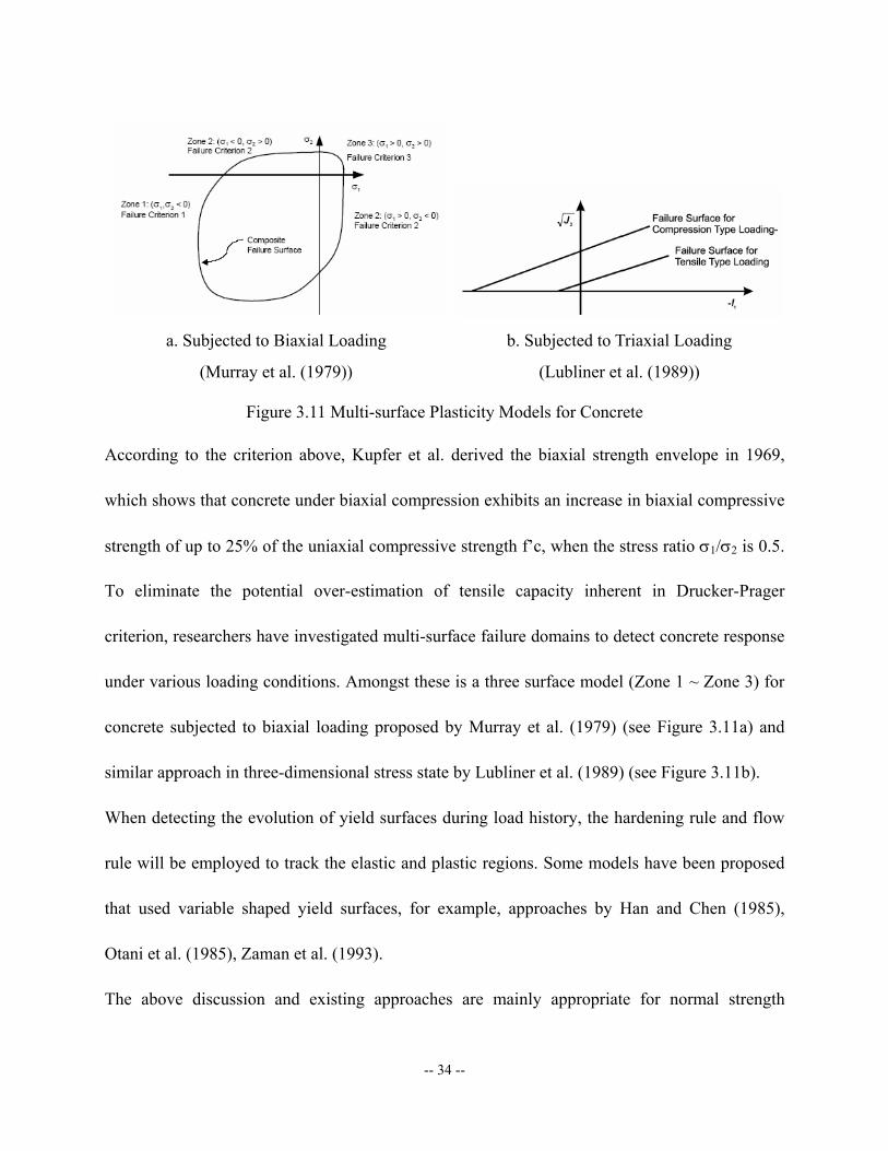
-- 34 --
a. Subjected to Biaxial Loading
(Murray et al. (1979))
b. Subjected to Triaxial Loading
(Lubliner et al. (1989))
Figure 3.11 Multi-surface Plasticity Models for Concrete
According to the criterion above, Kupfer et al. derived the biaxial strength envelope in 1969,
which shows that concrete under biaxial compression exhibits an increase in biaxial compressive
strength of up to 25% of the uniaxial compressive strength f’c, when the stress ratio σ1/σ2 is 0.5.
To eliminate the potential over-estimation of tensile capacity inherent in Drucker-Prager
criterion, researchers have investigated multi-surface failure domains to detect concrete response
under various loading conditions. Amongst these is a three surface model (Zone 1 ~ Zone 3) for
concrete subjected to biaxial loading proposed by Murray et al. (1979) (see Figure 3.11a) and
similar approach in three-dimensional stress state by Lubliner et al. (1989) (see Figure 3.11b).
When detecting the evolution of yield surfaces during load history, the hardening rule and flow
rule will be employed to track the elastic and plastic regions. Some models have been proposed
that used variable shaped yield surfaces, for example, approaches by Han and Chen (1985),
Otani et al. (1985), Zaman et al. (1993).
The above discussion and existing approaches are mainly appropriate for normal strength
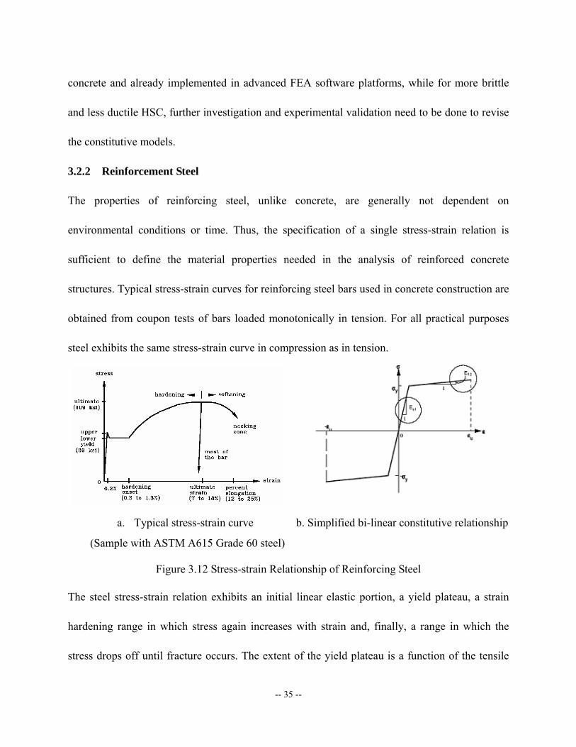
-- 35 --
concrete and already implemented in advanced FEA software platforms, while for more brittle
and less ductile HSC, further investigation and experimental validation need to be done to revise
the constitutive models.
3.2.2 Reinforcement Steel
The properties of reinforcing steel, unlike concrete, are generally not dependent on
environmental conditions or time. Thus, the specification of a single stress-strain relation is
sufficient to define the material properties needed in the analysis of reinforced concrete
structures. Typical stress-strain curves for reinforcing steel bars used in concrete construction are
obtained from coupon tests of bars loaded monotonically in tension. For all practical purposes
steel exhibits the same stress-strain curve in compression as in tension.
a. Typical stress-strain curve
(Sample with ASTM A615 Grade 60 steel)
b. Simplified bi-linear constitutive relationship
Figure 3.12 Stress-strain Relationship of Reinforcing Steel
The steel stress-strain relation exhibits an initial linear elastic portion, a yield plateau, a strain
hardening range in which stress again increases with strain and, finally, a range in which the
stress drops off until fracture occurs. The extent of the yield plateau is a function of the tensile

-- 36 --
strength of steel. High-strength, high-carbon steels, generally, have a much shorter yield plateau
than relatively low-strength, low-carbon steels. In this study the reinforcing steel is modeled as a
linear elastic, linear strain hardening material with yield stress σy, as shown in Figure 3.12a and
3.12b.
3.3 Beam-Column Members and Wall Panel
Design guidelines for RC high-rise buildings usually assume that the structural wall or core
system serve as the main resisting structure for lateral loads, while use beam-column frames to
support the gravity loads. This is generally reasonable since columns and beams generally
possess lower flexural and shear strengths than structural walls, and higher deformation capacity
than the latter. In the mechanism of reinforced concrete, beam and columns are also different
from the wall panels, especially in the influencing factors of shear, crack patterns and plastic
zone developments.
3.3.1 Beam-Column Members
3.3.1.1 Beam Model with Fiber-Based Sectional Approach
Timoshenko beam theory is the theoretical base for the analysis of RC beams and columns in the
present study, as shown in Figure 3.13, with following basics considered:
• The cross section will remain plane as rotating under bending
• Tension stress in concrete will be calculated by available formula using average tensile
strain along the member.
• Not only material inelasticity but also geometric nonlinearity (especially for columns)
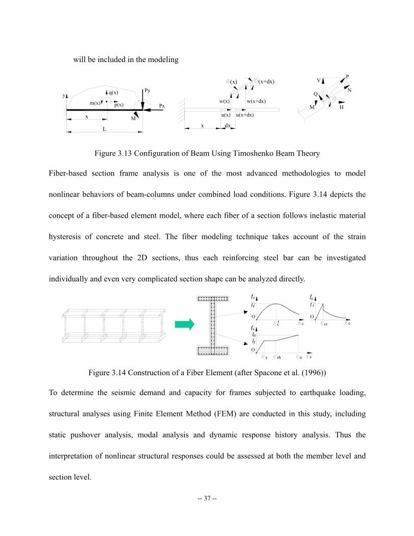
-- 37 --
will be included in the modeling
Px
q(x)
p(x)
L
x
w(x)
u(x)
x
w(x+dx)
u(x+dx)
dx
(x) (x+dx)
m(x)y
Py
M
V
HM
QN
P
Figure 3.13 Configuration of Beam Using Timoshenko Beam Theory
Fiber-based section frame analysis is one of the most advanced methodologies to model
nonlinear behaviors of beam-columns under combined load conditions. Figure 3.14 depicts the
concept of a fiber-based element model, where each fiber of a section follows inelastic material
hysteresis of concrete and steel. The fiber modeling technique takes account of the strain
variation throughout the 2D sections, thus each reinforcing steel bar can be investigated
individually and even very complicated section shape can be analyzed directly.
cr c
fc
O
tf '
'
f 'c
O
cf
cc
sh s
fs
O
yf
y u
f u
Figure 3.14 Construction of a Fiber Element (after Spacone et al. (1996))
To determine the seismic demand and capacity for frames subjected to earthquake loading,
structural analyses using Finite Element Method (FEM) are conducted in this study, including
static pushover analysis, modal analysis and dynamic response history analysis. Thus the
interpretation of nonlinear structural responses could be assessed at both the member level and
section level.
-- 38 --
3.3.1.2 ZEUS-NL Application
The Mid-America Earthquake Center analysis environment ZEUS-NL (Elnashai et al. (2002)) is
the principal computational tool for the 2D and 3D analysis needs of frames employed in this
research. As a promising frame analysis platform, ZEUS-NL has been developed over the past 16
years and used. It is a third generation 3D frame analysis platform, being a development of the
programs ADAPTIC (Izzuddin and Elnashai (1989)) and INDYAS (Elnashai et al. (2000)).
In ZEUS-NL, elements capable of modeling material and geometric nonlinearity are available.
The sectional force-displacement and moment-rotation responses are obtained through
integration of inelastic material responses of individual fibers describing the section. The
Eularian approach towards geometric nonlinearity is employed at the element level. Therefore,
full account is taken of the spread of inelasticity along the member length and across the section
depth as well as the effect of large member deformations. Since the sectional response is
calculated at each loading step from inelastic material models that account for stiffness and
strength degradation, there is no need for sweeping assumptions on the moment-curvature
relationships as required in other analysis approaches. In ZEUS-NL, conventional pushover,
adaptive pushover, Eigen analysis, and dynamic analyses are available that have been tested at
the member and structural levels. And axial-shear interaction effects can be taken into account
using nonlinear springs (Lee and Elnashai (2002)).
In this study, pushover analysis is executed for load-capacity curves and dynamic response
history analysis (DRHA) is in demand for numerical simulations to obtain fragility relationships.
ZEUS-NL is chosen as the main analytical platform for selected sample structures.
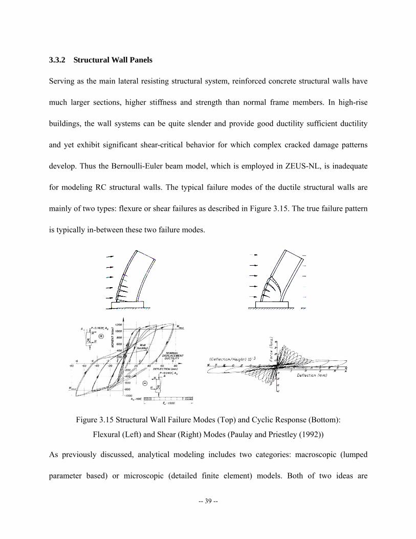
-- 39 --
3.3.2 Structural Wall Panels
Serving as the main lateral resisting structural system, reinforced concrete structural walls have
much larger sections, higher stiffness and strength than normal frame members. In high-rise
buildings, the wall systems can be quite slender and provide good ductility sufficient ductility
and yet exhibit significant shear-critical behavior for which complex cracked damage patterns
develop. Thus the Bernoulli-Euler beam model, which is employed in ZEUS-NL, is inadequate
for modeling RC structural walls. The typical failure modes of the ductile structural walls are
mainly of two types: flexure or shear failures as described in Figure 3.15. The true failure pattern
is typically in-between these two failure modes.
Figure 3.15 Structural Wall Failure Modes (Top) and Cyclic Response (Bottom):
Flexural (Left) and Shear (Right) Modes (Paulay and Priestley (1992))
As previously discussed, analytical modeling includes two categories: macroscopic (lumped
parameter based) or microscopic (detailed finite element) models. Both of two ideas are
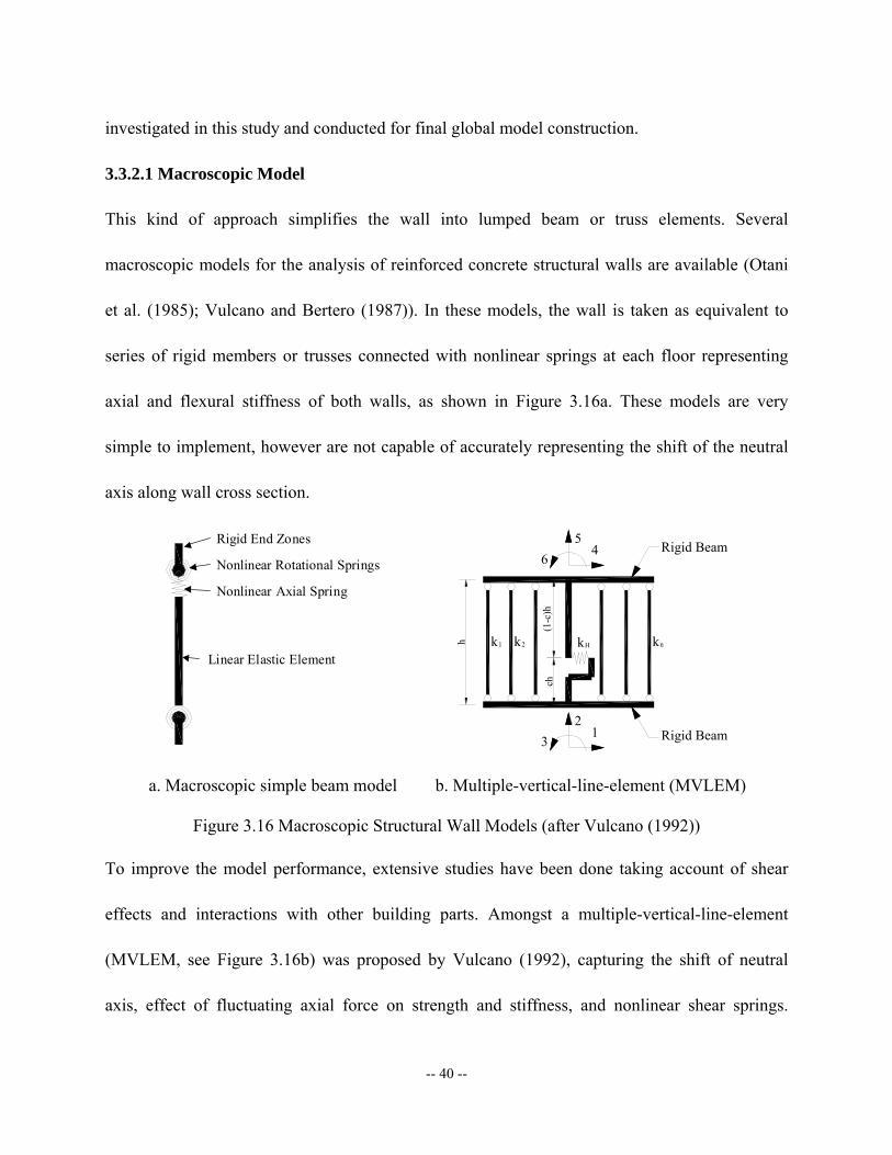
-- 40 --
investigated in this study and conducted for final global model construction.
3.3.2.1 Macroscopic Model
This kind of approach simplifies the wall into lumped beam or truss elements. Several
macroscopic models for the analysis of reinforced concrete structural walls are available (Otani
et al. (1985); Vulcano and Bertero (1987)). In these models, the wall is taken as equivalent to
series of rigid members or trusses connected with nonlinear springs at each floor representing
axial and flexural stiffness of both walls, as shown in Figure 3.16a. These models are very
simple to implement, however are not capable of accurately representing the shift of the neutral
axis along wall cross section.
Rigid End Zones
Nonlinear Rotational Springs
Nonlinear Axial Spring
Linear Elastic Element
k1 2k Hk nk
ch(1
-c)h
12
3
Rigid Beam
Rigid Beam
65
4
h
a. Macroscopic simple beam model b. Multiple-vertical-line-element (MVLEM)
Figure 3.16 Macroscopic Structural Wall Models (after Vulcano (1992))
To improve the model performance, extensive studies have been done taking account of shear
effects and interactions with other building parts. Amongst a multiple-vertical-line-element
(MVLEM, see Figure 3.16b) was proposed by Vulcano (1992), capturing the shift of neutral
axis, effect of fluctuating axial force on strength and stiffness, and nonlinear shear springs.
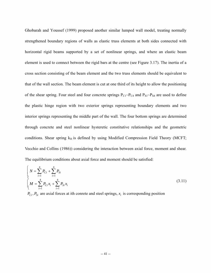
-- 41 --
Ghobarah and Youssef (1999) proposed another similar lumped wall model, treating normally
strengthened boundary regions of walls as elastic truss elements at both sides connected with
horizontal rigid beams supported by a set of nonlinear springs, and where an elastic beam
element is used to connect between the rigid bars at the centre (see Figure 3.17). The inertia of a
cross section consisting of the beam element and the two truss elements should be equivalent to
that of the wall section. The beam element is cut at one third of its height to allow the positioning
of the shear spring. Four steel and four concrete springs PC1~PC4 and PS1~PS4 are used to define
the plastic hinge region with two exterior springs representing boundary elements and two
interior springs representing the middle part of the wall. The four bottom springs are determined
through concrete and steel nonlinear hysteretic constitutive relationships and the geometric
conditions. Shear spring kH is defined by using Modified Compression Field Theory (MCFT;
Vecchio and Collins (1986)) considering the interaction between axial force, moment and shear.
The equilibrium conditions about axial force and moment should be satisfied:
4 4
1 14 4
1 1
, are axial forces at ith conrete and steel springs, is corresponding position
Ci Sii i
Ci i Si ii i
Ci Si i
N P P
M P x P x
P P x
= =
= =
⎧= +⎪
⎪⎨⎪ = +⎪⎩
∑ ∑
∑ ∑ (3.11)
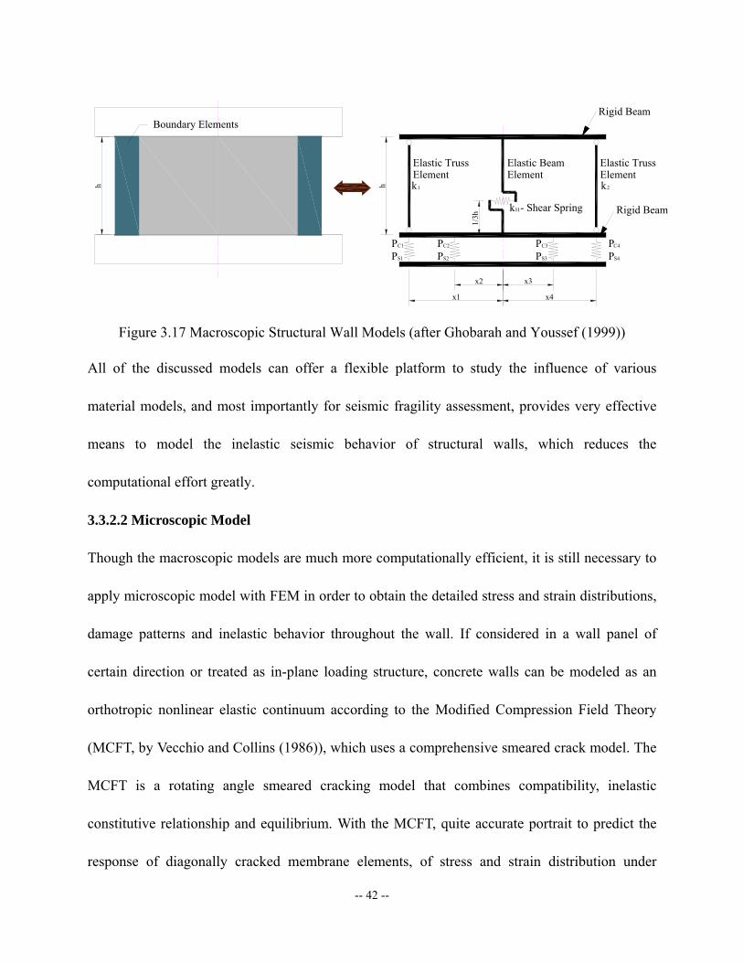
-- 42 --
Elastic TrussElement Element
Elastic Truss
PC1
S1P PS4
C4PPS2
C2P PC3
S3P
x1 x4
x2 x3
Boundary Elements
h
Elastic BeamElement
Rigid Beam
Rigid Beam
1/3h
k2
k - Shear SpringH
1kh
Figure 3.17 Macroscopic Structural Wall Models (after Ghobarah and Youssef (1999))
All of the discussed models can offer a flexible platform to study the influence of various
material models, and most importantly for seismic fragility assessment, provides very effective
means to model the inelastic seismic behavior of structural walls, which reduces the
computational effort greatly.
3.3.2.2 Microscopic Model
Though the macroscopic models are much more computationally efficient, it is still necessary to
apply microscopic model with FEM in order to obtain the detailed stress and strain distributions,
damage patterns and inelastic behavior throughout the wall. If considered in a wall panel of
certain direction or treated as in-plane loading structure, concrete walls can be modeled as an
orthotropic nonlinear elastic continuum according to the Modified Compression Field Theory
(MCFT, by Vecchio and Collins (1986)), which uses a comprehensive smeared crack model. The
MCFT is a rotating angle smeared cracking model that combines compatibility, inelastic
constitutive relationship and equilibrium. With the MCFT, quite accurate portrait to predict the
response of diagonally cracked membrane elements, of stress and strain distribution under
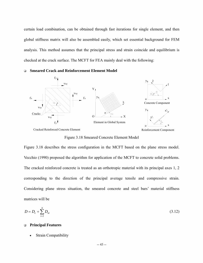
-- 43 --
certain load combination, can be obtained through fast iterations for single element, and then
global stiffness matrix will also be assembled easily, which set essential background for FEM
analysis. This method assumes that the principal stress and strain coincide and equilibrium is
checked at the crack surface. The MCFT for FEA mainly deal with the following:
Smeared Crack and Reinforcement Element Model
Cracked Reinforced Concrete Element
fy
fx
vxy
vxy
vxy
fy
fx
vxy
Cracks
Y
O X
y
o
xo
y
x
o x
y
12
y'i
x'i
iElement in Global System
Concrete Component
Reinforcement Component Figure 3.18 Smeared Concrete Element Model
Figure 3.18 describes the stress configuration in the MCFT based on the plane stress model.
Vecchio (1990) proposed the algorithm for application of the MCFT to concrete solid problems.
The cracked reinforced concrete is treated as an orthotropic material with its principal axes 1, 2
corresponding to the direction of the principal average tensile and compressive strain.
Considering plane stress situation, the smeared concrete and steel bars’ material stiffness
matrices will be
1
n
c sii
D D D=
= +∑ (3.12)
Principal Features
• Strain Compatibility
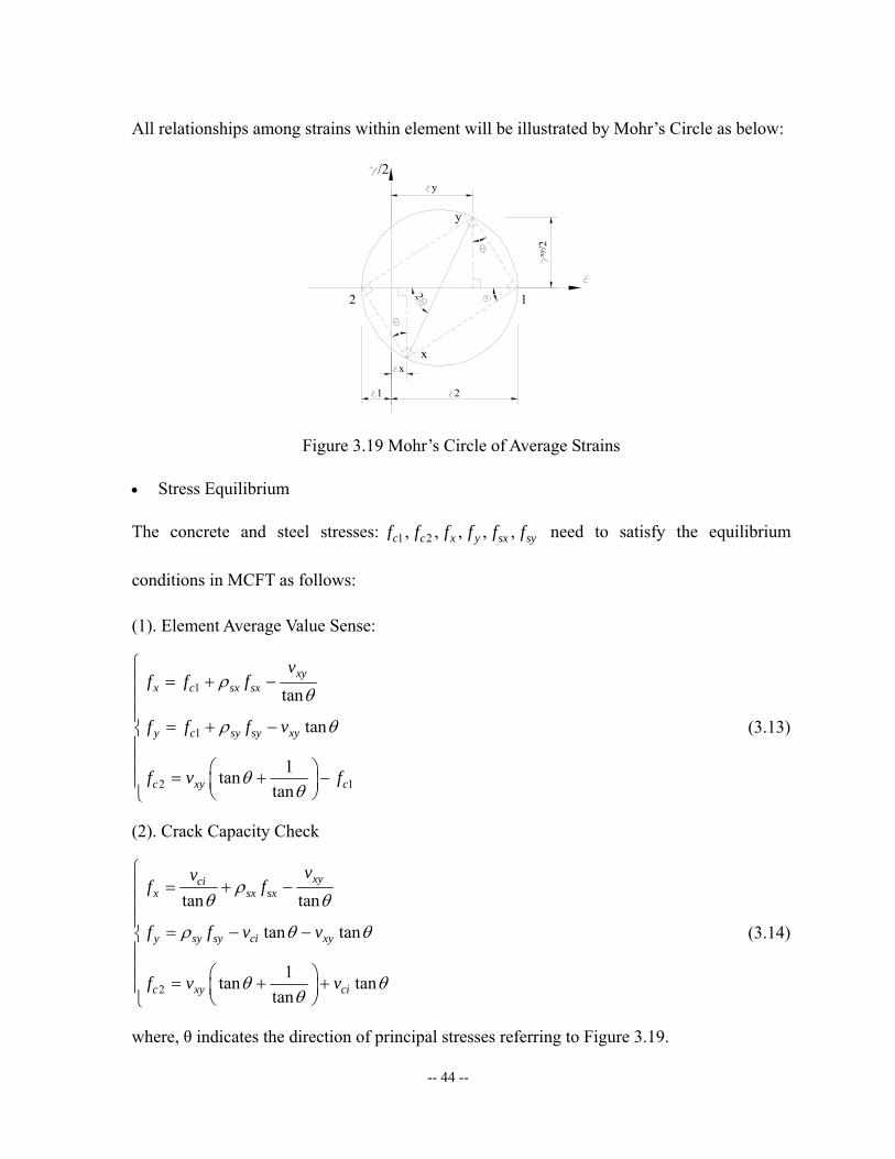
-- 44 --
All relationships among strains within element will be illustrated by Mohr’s Circle as below:
x
1 2
12
x
y
2
/2y
xy/2
Figure 3.19 Mohr’s Circle of Average Strains
• Stress Equilibrium
The concrete and steel stresses: 1 2, , , , ,c c x y sx syf f f f f f need to satisfy the equilibrium
conditions in MCFT as follows:
(1). Element Average Value Sense:
1
1
2 1
tan
tan
1tantan
xyx c sx sx
y c sy sy xy
c xy c
vf f f
f f f v
f v f
ρθ
ρ θ
θθ
⎧⎪ = + −⎪⎪
= + −⎨⎪⎪ ⎛ ⎞= + −⎪ ⎜ ⎟
⎝ ⎠⎩
(3.13)
(2). Crack Capacity Check
2
tan tan
tan tan
1tan tantan
xycix sx sx
y sy sy ci xy
c xy ci
vvf f
f f v v
f v v
ρθ θ
ρ θ θ
θ θθ
⎧⎪ = + −⎪⎪
= − −⎨⎪⎪ ⎛ ⎞= + +⎪ ⎜ ⎟
⎝ ⎠⎩
(3.14)
where, θ indicates the direction of principal stresses referring to Figure 3.19.
-- 45 --
3.3.2.3 VecTor2 Application
The inelastic 2D continuum analysis tool VecTor2 (developed at University of Toronto, Vecchio
(1990), Wong and Vecchio (2002)) was used to provide the predicted behavior of structural walls
in high-rise buildings. VecTor2 employs a rotating-angle smeared crack modeling approach and
implements both the MCFT and Disturbed Stress Field Model (DSFM) by Vecchio (2000).
The main difference and improvement from MCFT to DSFM lies in the including of shear slip
deformation at the cracks. This leads to the differences between the directions of the principal
stress and principal strain fields, hence distinguishing strains due to shear slip from the concrete
strains due to stress, which relates the stress and strain by constitutive relationships in a more
direct and reliable way. In addition, the shear check required in MCFT is eliminated in the
DSFM.
VecTor2 utilizes an iterative secant stiffness algorithm to produce an efficient and robust
nonlinear solution technique, with considerations of compression softening and tension stiffening.
It can model concrete expansion and confinement, cyclic loading and hysteretic response,
construction and loading chronology for repair applications, bond slip, crack shear slip
deformations, reinforcement dowel action, reinforcement buckling, and crack allocation
processes.
Finite element models constructed for VecTor2 use a fine mesh of low-powered elements. This
methodology has advantages of computational efficiency and numerical stability. It is also well
suited to reinforced concrete structures, which require a relatively fine mesh to model
reinforcement detailing and 3 local crack patterns. The element library includes a three-node
-- 46 --
constant strain triangle, a four-node plane stress rectangular element and a four-node
quadrilateral element for modeling concrete with smeared reinforcement; a two-node truss-bar
for modeling discrete reinforcement; and a two-node link and a four-node contact element for
modeling bond-slip mechanisms.
3.3.2.4 Necessity of Lumped-Parameter-Based Modeling
Required by the analytically based seismic fragility assessment, a great many simulations and
dynamic analyses must be executed for selected RC high-rise buildings. It is not practical to
employ microscopic wall model with continuum FEM for each analysis, e.g. it usually takes
more than 2 hours to run one nonlinear DRHA for a RC fiber-based model with more than 1000
beam elements using normal ground motion records. Hundreds of DRHA for analytical fragility
assessment would require prohibitively long analysis time. Therefore appropriate
lumped-parameter based structural model is one of the major objectives in this study. Referring
to the existing lumped models, enhanced simplification techniques are under investigation with
the following concerns:
• Simulation of M-N-V interaction
• Constitutive relationships for both normal and high-strength concrete
• Position of shear springs
• Model validation
The computational tool for lumped model will be ZEUS-NL where the final model will consist
of beam elements, rigid bars and nonlinear springs. The lumped model will be constructed and
refined using mathematical parametric studies on critical joint and spring constants. Both

-- 47 --
ZEUS-NL and VecTor2 are used for this process.
3.3.3 Wall-Frame Interaction
Under lateral earthquake loads, the common frame-wall interaction varies along the height of the
structure; it also depends upon the type and the stiffness of structural components used to
connect the two components of the high-rise buildings, e.g. coupling beams with rigid or
semi-rigid connections. Shear racking from the frame and flexural bending from the wall
primarily generate the lateral structural deformations. Frame lateral displacements reduce as the
height increases; conversely, lateral deflections of braced frames and structural walls increase
with the height. This difference in lateral stiffness along the height between the structural
components significantly affects the distribution of seismic actions. The shear resisted by the
frame increase with the height, while decrease for the interacting wall.
An accurate way to detect the wall-frame interaction is to build detailed FEM models for all
structural components, e.g., whole 3D building model with brick elements in ABAQUS. Then
the load transfer and redistributions due to different inelastic behavior of different components
can be observed and investigated throughout the structure. However the major weakness of this
approach is the great computational cost caused by large number of elements and complex
nonlinear algorithms required in detailed finite element analyses (FEA). There exist more
feasible alternative approaches for the structural modeling by:
• Using beam elements for wall and frame components to form 2D or 3D lumped frame model
of the whole structure; for example, 3D frame analysis in ZEUS-NL with fiber-based
sectional approach.
-- 48 --
• Performing multi-stage FEA, in which a frame model for the whole building is used first and
then structural components like wall and frame are analyzed separately in different
compatible models with load histories applied on the interfaces obtained from the previous
stage results. Through sets of parametric studies, equivalent lumped models for walls and
wall-frame interfaces can be derived and integrated into a new simplified structural model for
the future analysis especially DRHA, including wall shear effects and wall-frame
interactions. This will serve as the main methodology for the derivation of the global
structural model for fragility assessment.
• Using a technique called multi-resolution distributed finite element analysis (MDFEA) for
the whole building. Different compatible FEM models for different divided sub-structural
components are employed in such way that the components subjected to the most complex
states of stress are modeled using detailed FE and the remaining parts are in computationally
efficient skeletal elements. This might be the most reliable and computationally efficient
method to analyze large complex structure. Unfortunately, many existing software do not
include all the best material models or finite elements. It is therefore natural to consider the
use of more than one analysis platform to make best use of their relative merits. The multiple
distinct applications can be combined within a multi-platform simulation framework in a
step-by-step fashion with the load history. MDFEA is described in details in section 4.2.
However there still exists a major inherent pullback – the huge runtime request of MDFEA
makes it impractical to be applied for large amount of simulations for fragility assessment at
this time.
-- 49 --
3.3.4 Verifications of Frame and Wall FEM Analysis Software
3.3.4.1 ZEUS-NL for Frame Analysis
As the major analysis platform in Mid-America Earthquake (MAE) Center, ZEUS-NL has been
used by many researchers from institutes and multiple areas. ZEUS-NL proved itself to be a
powerful, accurate and reliable 3D frame FEA software.
During the development, many verifications and enhancements have been executed for
ZEUS-NL by the original developers and other researchers. The uniaxial nonlinear constant
confinement model was derived by Martinez-Rueda and Elnashai (1997) according to
constitutive relationship proposed by Mander et al. (1988) for reasons of numerical stability
under large displacements analysis. Pinho et al. (2000) used the application to analyze a
full-scale reinforced concrete frame that was tested using the pseudo-dynamic approach at the
ELSA laboratory at JRC (Ispra, Italy). The results proved that the experimental response of the
model did follow the behavior numerically predicted prior to the test. Most recently, Jeong and
Elnashai (2004a) used ZEUS-NL to assess the seismic response of a full-scale 3D RC frame
testing structure, showing the blind predictions to be accurate and representative of the
subsequence pseudo-dynamic test. Kwon and Elnashai (2005) verified the structural model and
analysis environment in ZEUS-NL through comparison of response history analysis with shake
table test by Bracci et al. (1992). The verification is undertaken for a multi-storey RC frame
building in terms of structural periods and global displacement history since local stress-strain
measurements are not available in the published literature.
Therefore ZEUS-NL is functional and reliable enough to meet the requirement of numerical
-- 50 --
simulations needed in fragility assessment.
3.3.4.2 VecTor2 for Wall Continuum Analysis
Existing Experimental Data
In the analytical modeling process VecTor2 will be used to serve as the primary analysis tool for
RC shear walls to include shear contributions and M-V-N interactions. As advanced FEM
software, VecTor2 have been widely employed by researchers for different kinds of RC
continuum structures, including predictions for large-scale experimental test specimens. Palermo
and Vecchio (2004) have verified the performances of VecTor2 for series of shear wall test
researches, such as Portland Cement Association (PCA) slender structural walls (Oesterle et al.
(1976)), O series wall specimens tested at the University of Ottawa (Wiradinata and Saatcioglu
2002), and DP walls tested by Palermo and Vecchio (2004). Multiple aspects, consist of concrete
and steel reverse cyclic constitutive relationships and FEM meshing, are investigated with the
evaluation of effects on FEA results and comparisons with experiment results from both global
responses and local RC behavior. It was concluded by Palermo and Vecchio (2004) that for both
squat and slender walls VecTor2 can handle the microscopic FEA very well and detailed
information from global deformation to local stress strain fields and crack propagation can be
collected accurately.
Due to the significance of structural wall performance in high-rise buildings, additional
verifications are conducted to evaluate VecTor2 from accuracy and stability aspects in this
research. Here, the results from two systematic large-scale shear wall experiments conducted by
other researchers are compared with the results from FEM analysis. For the purpose of
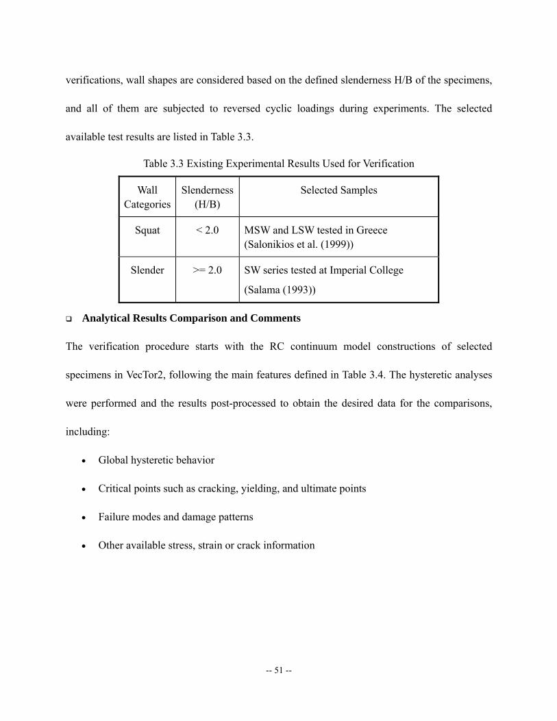
-- 51 --
verifications, wall shapes are considered based on the defined slenderness H/B of the specimens,
and all of them are subjected to reversed cyclic loadings during experiments. The selected
available test results are listed in Table 3.3.
Table 3.3 Existing Experimental Results Used for Verification
Wall Categories
Slenderness (H/B)
Selected Samples
Squat < 2.0 MSW and LSW tested in Greece (Salonikios et al. (1999))
Slender >= 2.0 SW series tested at Imperial College
(Salama (1993))
Analytical Results Comparison and Comments
The verification procedure starts with the RC continuum model constructions of selected
specimens in VecTor2, following the main features defined in Table 3.4. The hysteretic analyses
were performed and the results post-processed to obtain the desired data for the comparisons,
including:
• Global hysteretic behavior
• Critical points such as cracking, yielding, and ultimate points
• Failure modes and damage patterns
• Other available stress, strain or crack information
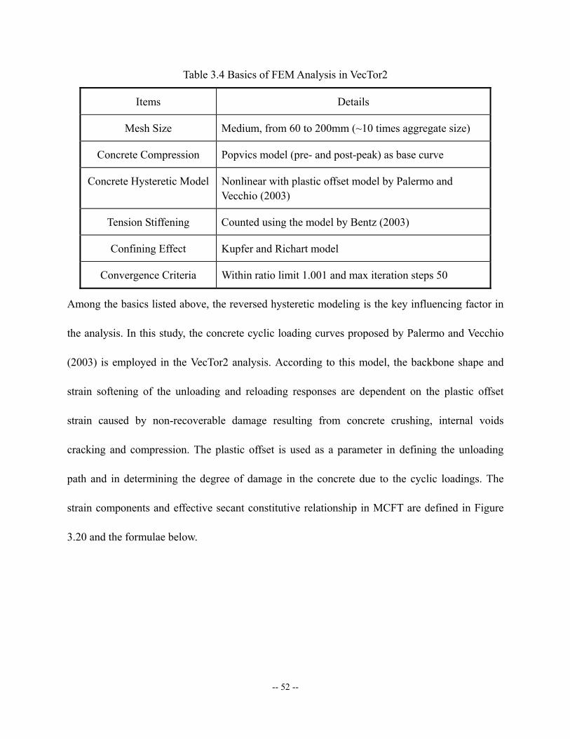
-- 52 --
Table 3.4 Basics of FEM Analysis in VecTor2
Items Details
Mesh Size Medium, from 60 to 200mm (~10 times aggregate size)
Concrete Compression Popvics model (pre- and post-peak) as base curve
Concrete Hysteretic Model Nonlinear with plastic offset model by Palermo and Vecchio (2003)
Tension Stiffening Counted using the model by Bentz (2003)
Confining Effect Kupfer and Richart model
Convergence Criteria Within ratio limit 1.001 and max iteration steps 50
Among the basics listed above, the reversed hysteretic modeling is the key influencing factor in
the analysis. In this study, the concrete cyclic loading curves proposed by Palermo and Vecchio
(2003) is employed in the VecTor2 analysis. According to this model, the backbone shape and
strain softening of the unloading and reloading responses are dependent on the plastic offset
strain caused by non-recoverable damage resulting from concrete crushing, internal voids
cracking and compression. The plastic offset is used as a parameter in defining the unloading
path and in determining the degree of damage in the concrete due to the cyclic loadings. The
strain components and effective secant constitutive relationship in MCFT are defined in Figure
3.20 and the formulae below.
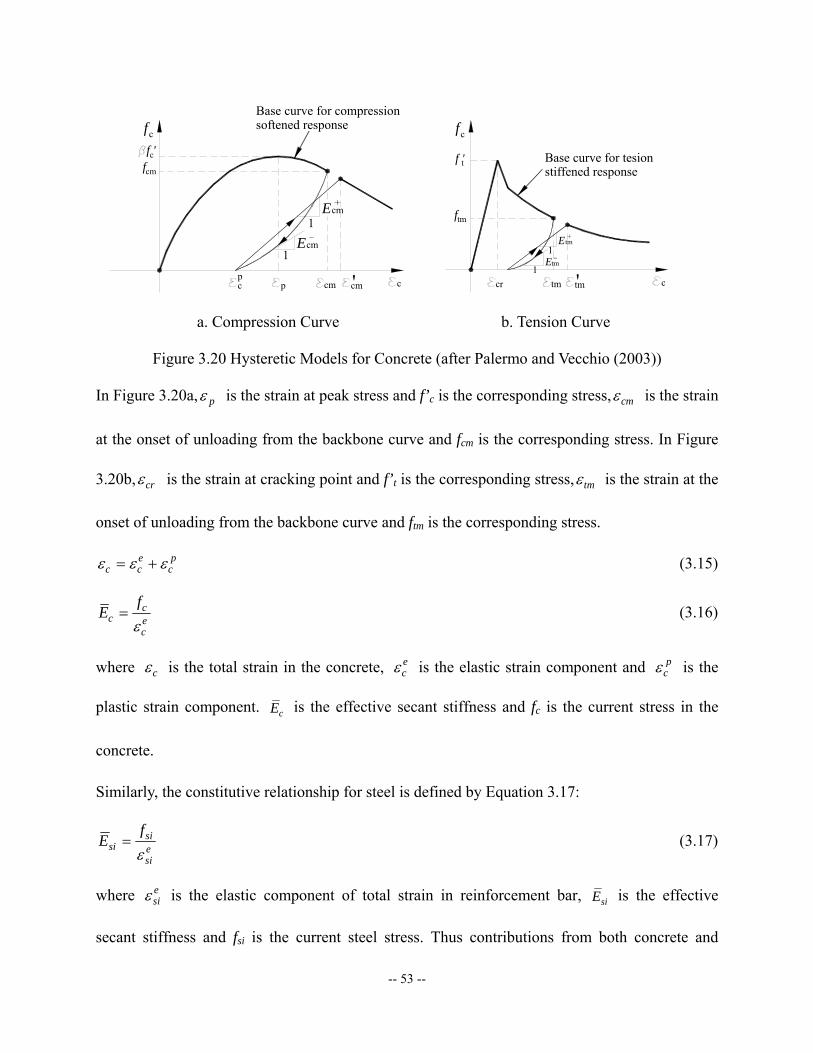
-- 53 --
softened responseBase curve for compression
'
cmf f 'c
cmE1
cf
ccmp cmpc
1Ecm
+
tmtm c
fc
1
tf '
f tm
'
Base curve for tesionstiffened response
E
+
tm1
Etm
cr
a. Compression Curve b. Tension Curve
Figure 3.20 Hysteretic Models for Concrete (after Palermo and Vecchio (2003))
In Figure 3.20a, pε is the strain at peak stress and f’c is the corresponding stress, cmε is the strain
at the onset of unloading from the backbone curve and fcm is the corresponding stress. In Figure
3.20b, crε is the strain at cracking point and f’t is the corresponding stress, tmε is the strain at the
onset of unloading from the backbone curve and ftm is the corresponding stress.
e pc c cε ε ε= + (3.15)
cc e
c
fE
ε= (3.16)
where cε is the total strain in the concrete, ecε is the elastic strain component and p
cε is the
plastic strain component. cE is the effective secant stiffness and fc is the current stress in the
concrete.
Similarly, the constitutive relationship for steel is defined by Equation 3.17:
sisi e
si
fE
ε= (3.17)
where esiε is the elastic component of total strain in reinforcement bar, siE is the effective
secant stiffness and fsi is the current steel stress. Thus contributions from both concrete and

-- 54 --
reinforcement are counted including plasticity.
• Compressive response
The important plastic offset strain pcε can be computed as following:
2
0.166 0.132p cm cmc p
p p
ε εε ε
ε ε
⎡ ⎤⎛ ⎞ ⎛ ⎞⎢ ⎥= +⎜ ⎟ ⎜ ⎟⎜ ⎟ ⎜ ⎟⎢ ⎥⎝ ⎠ ⎝ ⎠⎣ ⎦
(3.18)
The unloading relationship of the model is expressed as:
( ) ( )( )( )
( )2 1
1 , with N
cm cmc cm c c cmNp
c cm
E Ef f E
N
εε ε ε ε ε
ε ε
− −
−
⎡ ⎤− Δ⎢ ⎥Δ = + Δ + Δ = −⎢ ⎥−⎢ ⎥⎣ ⎦
(3.19)
where 1cmE− is the initial unloading stiffness assumed to be equal to the elastic tangent stiffness
of concrete cE , 2cmE− is the end unloading stiffness assumed to be equal to 0.071 cE , and N is
the Ramberg-Osgood power term computed as below:
( )( )( )
1 2
1
pcm cm c cm
pcm cm c cm
E EN
f E
ε ε
ε ε
− −
−
− −=
+ − (3.20)
For the reloading branch, linear relationship degrading by increasing load cycles is proposed in
the employed model. The reloading response can be expressed as:
( ) ( ) , with c ro cm c rof f Eε ε ε ε ε+Δ = + Δ Δ = − (3.21)
where rof is the initial reloading stress and roε is the initial reloading strain. Reloading
stiffness cmE+ is computed as:
( )maxd rocm
cm ro
f fE
βε ε
+ −=
− (3.22)
Here, dβ is a damage indicator defined to count the degradation of strength by the load cycling.
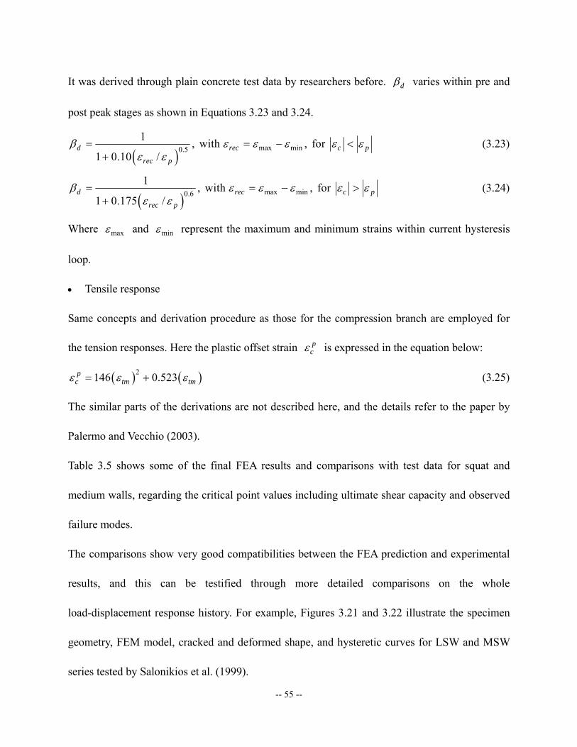
-- 55 --
It was derived through plain concrete test data by researchers before. dβ varies within pre and
post peak stages as shown in Equations 3.23 and 3.24.
( )max min0.5
1 , with , for 1 0.10 /
d rec c p
rec p
β ε ε ε ε εε ε
= = − <+
(3.23)
( )max min0.6
1 , with , for 1 0.175 /
d rec c p
rec p
β ε ε ε ε εε ε
= = − >+
(3.24)
Where maxε and minε represent the maximum and minimum strains within current hysteresis
loop.
• Tensile response
Same concepts and derivation procedure as those for the compression branch are employed for
the tension responses. Here the plastic offset strain pcε is expressed in the equation below:
( ) ( )2146 0.523pc tm tmε ε ε= + (3.25)
The similar parts of the derivations are not described here, and the details refer to the paper by
Palermo and Vecchio (2003).
Table 3.5 shows some of the final FEA results and comparisons with test data for squat and
medium walls, regarding the critical point values including ultimate shear capacity and observed
failure modes.
The comparisons show very good compatibilities between the FEA prediction and experimental
results, and this can be testified through more detailed comparisons on the whole
load-displacement response history. For example, Figures 3.21 and 3.22 illustrate the specimen
geometry, FEM model, cracked and deformed shape, and hysteretic curves for LSW and MSW
series tested by Salonikios et al. (1999).

-- 56 --
Table 3.5 FEA Results by VecTor2 and Comparisons with Test Data
Specimen B/H fcc (Mpa) Vu (Experiment) (kN)
Vu (VecTor2) (kN)
Difference (%) Failure Mode
SW4 2 49.5 108 110.9 2.69 FlexureSW9 2 53.7 101 110.3 9.21 FlexureSW22 2 45.1 98.7 111.0 12.46 FlexureSW23 2 47.4 123 130.6 6.18 FlexureSW31 2 46.4 62 64.4 3.87 Flexure
(Tested walls by Salama and Elnashai, 1993)
Specimen B/H f'c (Mpa) Vu (Experiment) (kN)
Vu (VecTor2) (kN)
Difference (%) Failure Mode
LSW1 1 22.2 262 284.3 8.51 Flexure-ShearLSW3 1 23.9 268 279.6 4.33 Flexure-ShearMSW1 1.5 26.1 197 198.2 0.61 FlexureMSW2 1.5 26.2 124 143.4 15.65 FlexureMSW3 1.5 24.1 176 195.7 11.19 Flexure
(Tested walls by Salonikios, Kappos, Tegos and Penelis, 1999)
a. Specimen Geometry vs. FEM Model b. Image vs. FEA Plot for Cracked Shape
-300
-200
-100
0
100
200
300
-30 -20 -10 0 10 20 30
Top Displacement Dx (mm)
Tota
l Loa
d Fx
(kN
)
LSW1
c. Test Data vs. FEA Results for Hysteretic Vbase-Dtop Curve
Figure 3.21 LSW1 Test Structure and Data vs. FEM Model and Analysis Results
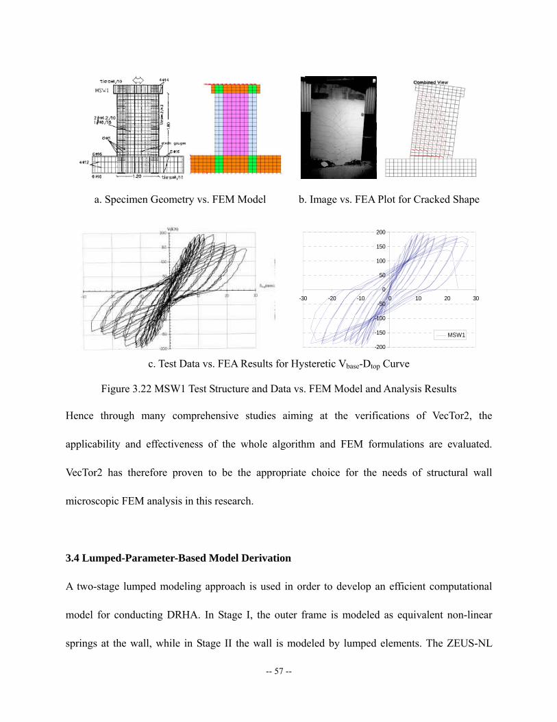
-- 57 --
a. Specimen Geometry vs. FEM Model b. Image vs. FEA Plot for Cracked Shape
-200
-150
-100
-50
0
50
100
150
200
-30 -20 -10 0 10 20 30(
)
MSW1
c. Test Data vs. FEA Results for Hysteretic Vbase-Dtop Curve
Figure 3.22 MSW1 Test Structure and Data vs. FEM Model and Analysis Results
Hence through many comprehensive studies aiming at the verifications of VecTor2, the
applicability and effectiveness of the whole algorithm and FEM formulations are evaluated.
VecTor2 has therefore proven to be the appropriate choice for the needs of structural wall
microscopic FEM analysis in this research.
3.4 Lumped-Parameter-Based Model Derivation
A two-stage lumped modeling approach is used in order to develop an efficient computational
model for conducting DRHA. In Stage I, the outer frame is modeled as equivalent non-linear
springs at the wall, while in Stage II the wall is modeled by lumped elements. The ZEUS-NL
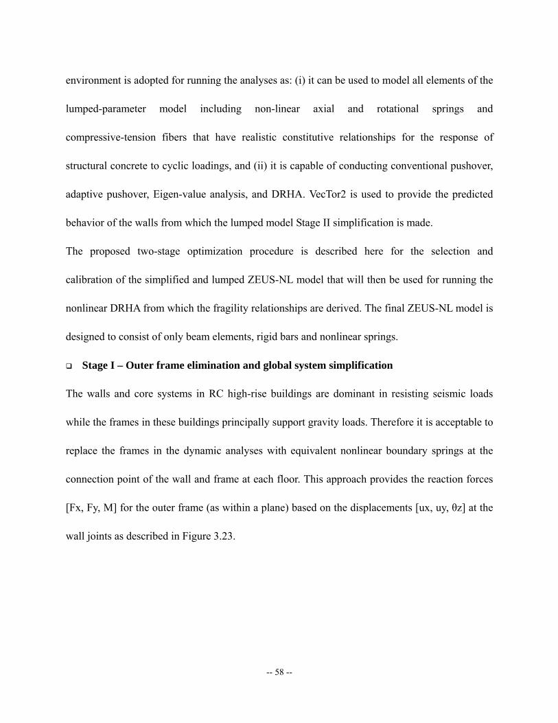
-- 58 --
environment is adopted for running the analyses as: (i) it can be used to model all elements of the
lumped-parameter model including non-linear axial and rotational springs and
compressive-tension fibers that have realistic constitutive relationships for the response of
structural concrete to cyclic loadings, and (ii) it is capable of conducting conventional pushover,
adaptive pushover, Eigen-value analysis, and DRHA. VecTor2 is used to provide the predicted
behavior of the walls from which the lumped model Stage II simplification is made.
The proposed two-stage optimization procedure is described here for the selection and
calibration of the simplified and lumped ZEUS-NL model that will then be used for running the
nonlinear DRHA from which the fragility relationships are derived. The final ZEUS-NL model is
designed to consist of only beam elements, rigid bars and nonlinear springs.
Stage I – Outer frame elimination and global system simplification
The walls and core systems in RC high-rise buildings are dominant in resisting seismic loads
while the frames in these buildings principally support gravity loads. Therefore it is acceptable to
replace the frames in the dynamic analyses with equivalent nonlinear boundary springs at the
connection point of the wall and frame at each floor. This approach provides the reaction forces
[Fx, Fy, M] for the outer frame (as within a plane) based on the displacements [ux, uy, θz] at the
wall joints as described in Figure 3.23.
-- 59 --
WallKxKr_z
Ky
Fixed
Joint Detail
1
2
3
( )Equivalent Outer Frame Model: ( )
( )Where, i - floor level;
, , - nodal displacements of core wall
i xi
i yi
i i
xi yi i
Fx f uFy f uM f
u u
θ
θ
⎧ ⎫⎧ ⎫⎪ ⎪⎪ ⎪ =⎨ ⎬ ⎨ ⎬
⎪ ⎪ ⎪ ⎪⎩ ⎭ ⎩ ⎭
⎡ ⎤⎣ ⎦
Figure 3.23 Equivalent Nonlinear Springs at Wall Joint
Stage II – Simplify the structural wall into lumped elements
It is possible to simplify the model for the wall into lumped elements that must be selected to
capture the nonlinear longitudinal behavior across the width of the wall as well as its shear
behavior. Two different simplified lumped models were used and are compared in this Stage II
optimization procedure. The simple-vertical-line-element model (SVLEM) shown in Figure
3.16a and a multiple-vertical-line-element model (MVLEM) is shown in Figure 3.17. Nonlinear
shear springs are added for both models introducing the shear deformation contributions to
enhance the ZEUS-NL beam modeling.
3.4.1 Methodology
While lumped-modeling approaches are conceptually simple, the selection of a suitable
replacement structure that properly considers the influence of the dominant parameters on the
nonlinear response is not trivial. The whole procedure is actually dominated by parametric
studies. There is no explicit analytical approach to derive this model from inelastic FEA and
direct optimization techniques for parametric studies are not appropriate since they all depend on
explicit functions. In this proposed framework and computational approach, implicit
methodologies that use Genetic Algorithm (GA) are applied.
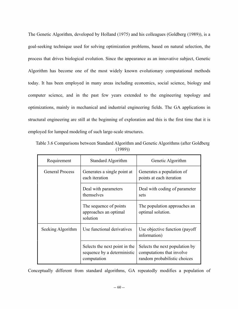
-- 60 --
The Genetic Algorithm, developed by Holland (1975) and his colleagues (Goldberg (1989)), is a
goal-seeking technique used for solving optimization problems, based on natural selection, the
process that drives biological evolution. Since the appearance as an innovative subject, Genetic
Algorithm has become one of the most widely known evolutionary computational methods
today. It has been employed in many areas including economics, social science, biology and
computer science, and in the past few years extended to the engineering topology and
optimizations, mainly in mechanical and industrial engineering fields. The GA applications in
structural engineering are still at the beginning of exploration and this is the first time that it is
employed for lumped modeling of such large-scale structures.
Table 3.6 Comparisons between Standard Algorithm and Genetic Algorithms (after Goldberg (1989))
Requirement Standard Algorithm Genetic Algorithm
Generates a single point at each iteration
Generates a population of points at each iteration
Deal with parameters themselves
Deal with coding of parameter sets
General Process
The sequence of points approaches an optimal solution
The population approaches an optimal solution.
Use functional derivatives Use objective function (payoff information)
Seeking Algorithm
Selects the next point in the sequence by a deterministic computation
Selects the next population by computations that involve random probabilistic choices
Conceptually different from standard algorithms, GA repeatedly modifies a population of
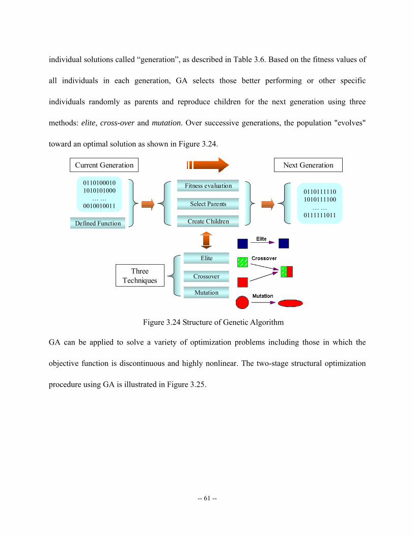
-- 61 --
individual solutions called “generation”, as described in Table 3.6. Based on the fitness values of
all individuals in each generation, GA selects those better performing or other specific
individuals randomly as parents and reproduce children for the next generation using three
methods: elite, cross-over and mutation. Over successive generations, the population "evolves"
toward an optimal solution as shown in Figure 3.24.
01101000101010101000
… …0010010011
Current Generation
01101111101010111100
… …0111111011
Next Generation
Elite
Fitness evaluation
Crossover
Mutation
Defined Function
Three Techniques
Select Parents
Create Children
Figure 3.24 Structure of Genetic Algorithm
GA can be applied to solve a variety of optimization problems including those in which the
objective function is discontinuous and highly nonlinear. The two-stage structural optimization
procedure using GA is illustrated in Figure 3.25.
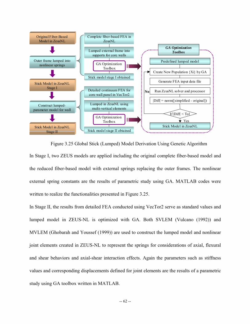
-- 62 --
Detailed continuum FEA for core wall panel in VecTor2
Lumped in ZeusNL using multi-vertical elements
Original Fiber-Based Model in ZeusNL
Stick Model in ZeusNL Stage I
Outer frame lumped into nonlinear springs
Stick Model in ZeusNL Stage II
Construct lumped-parameter model for wall
GA Optimization Toolbox
Predefined lumped model
Create New Population {Xi} by GA
Stick Model in ZeusNL
Generate FEA input data file
Run ZeusNL solver and processor
If |Diff| < Tol
|Diff| = norm([simplified - original])
No
Yes
GA Optimization Toolbox
Complete fiber-based FEA in ZeusNL
Lumped external frame into supports for core walls
GA Optimization Toolbox
Stick model stage I obtained
Stick model stage II obtained
Figure 3.25 Global Stick (Lumped) Model Derivation Using Genetic Algorithm
In Stage I, two ZEUS models are applied including the original complete fiber-based model and
the reduced fiber-based model with external springs replacing the outer frames. The nonlinear
external spring constants are the results of parametric study using GA. MATLAB codes were
written to realize the functionalities presented in Figure 3.25.
In Stage II, the results from detailed FEA conducted using VecTor2 serve as standard values and
lumped model in ZEUS-NL is optimized with GA. Both SVLEM (Vulcano (1992)) and
MVLEM (Ghobarah and Youssef (1999)) are used to construct the lumped model and nonlinear
joint elements created in ZEUS-NL to represent the springs for considerations of axial, flexural
and shear behaviors and axial-shear interaction effects. Again the parameters such as stiffness
values and corresponding displacements defined for joint elements are the results of a parametric
study using GA toolbox written in MATLAB.
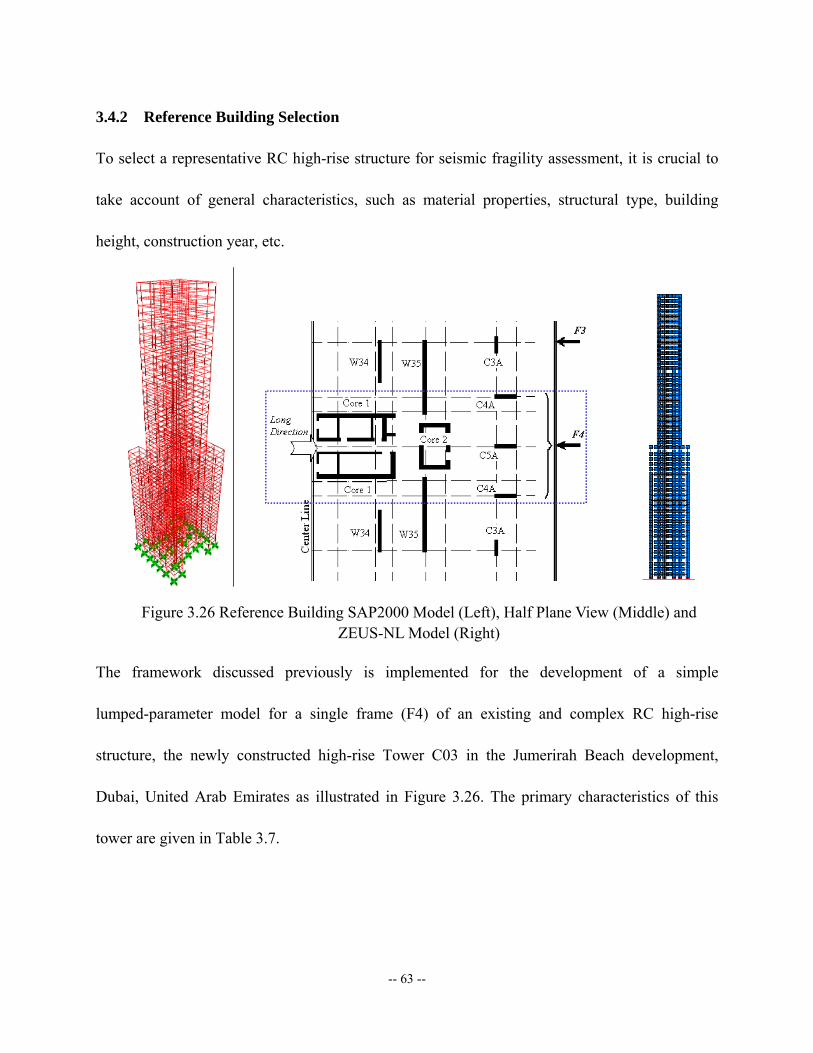
-- 63 --
3.4.2 Reference Building Selection
To select a representative RC high-rise structure for seismic fragility assessment, it is crucial to
take account of general characteristics, such as material properties, structural type, building
height, construction year, etc.
Figure 3.26 Reference Building SAP2000 Model (Left), Half Plane View (Middle) and ZEUS-NL Model (Right)
The framework discussed previously is implemented for the development of a simple
lumped-parameter model for a single frame (F4) of an existing and complex RC high-rise
structure, the newly constructed high-rise Tower C03 in the Jumerirah Beach development,
Dubai, United Arab Emirates as illustrated in Figure 3.26. The primary characteristics of this
tower are given in Table 3.7.
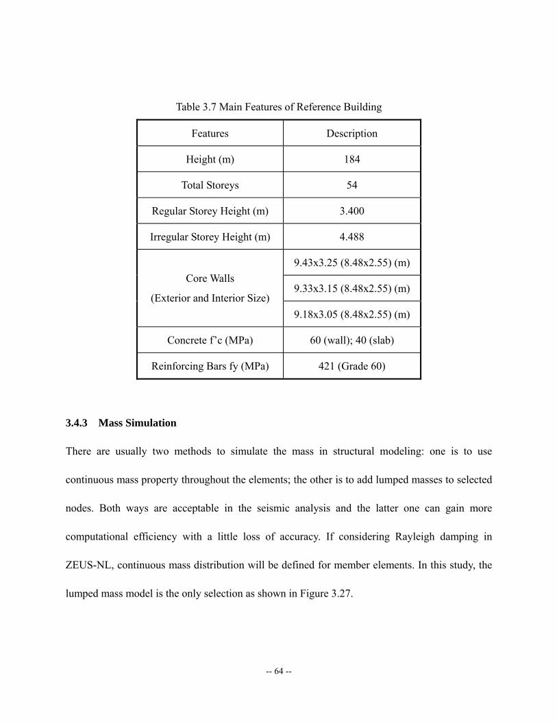
-- 64 --
Table 3.7 Main Features of Reference Building
Features Description
Height (m) 184
Total Storeys 54
Regular Storey Height (m) 3.400
Irregular Storey Height (m) 4.488
9.43x3.25 (8.48x2.55) (m)
9.33x3.15 (8.48x2.55) (m) Core Walls
(Exterior and Interior Size) 9.18x3.05 (8.48x2.55) (m)
Concrete f’c (MPa) 60 (wall); 40 (slab)
Reinforcing Bars fy (MPa) 421 (Grade 60)
3.4.3 Mass Simulation
There are usually two methods to simulate the mass in structural modeling: one is to use
continuous mass property throughout the elements; the other is to add lumped masses to selected
nodes. Both ways are acceptable in the seismic analysis and the latter one can gain more
computational efficiency with a little loss of accuracy. If considering Rayleigh damping in
ZEUS-NL, continuous mass distribution will be defined for member elements. In this study, the
lumped mass model is the only selection as shown in Figure 3.27.
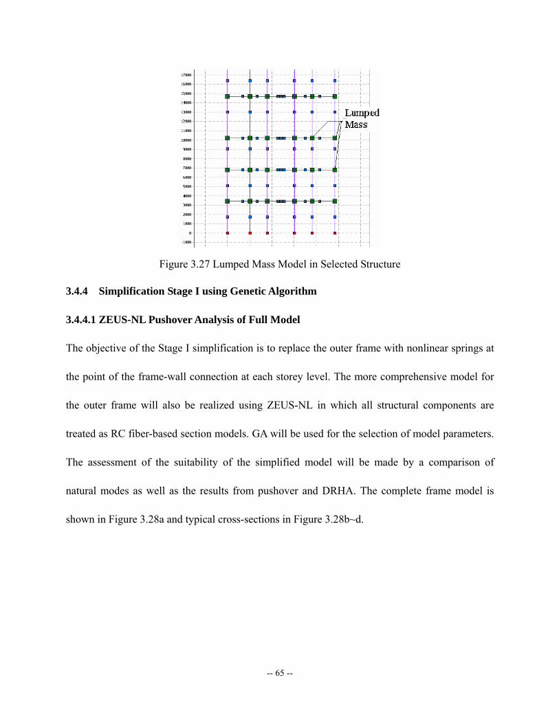
-- 65 --
Figure 3.27 Lumped Mass Model in Selected Structure
3.4.4 Simplification Stage I using Genetic Algorithm
3.4.4.1 ZEUS-NL Pushover Analysis of Full Model
The objective of the Stage I simplification is to replace the outer frame with nonlinear springs at
the point of the frame-wall connection at each storey level. The more comprehensive model for
the outer frame will also be realized using ZEUS-NL in which all structural components are
treated as RC fiber-based section models. GA will be used for the selection of model parameters.
The assessment of the suitability of the simplified model will be made by a comparison of
natural modes as well as the results from pushover and DRHA. The complete frame model is
shown in Figure 3.28a and typical cross-sections in Figure 3.28b~d.
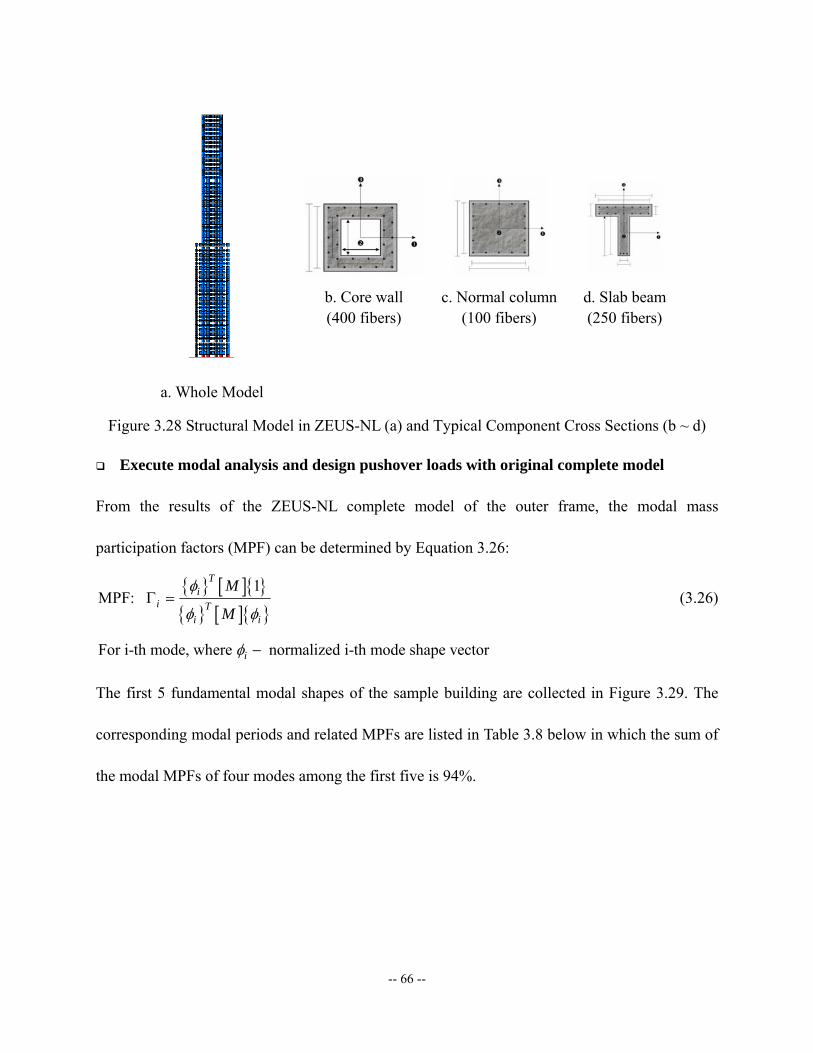
-- 66 --
a. Whole Model
b. Core wall (400 fibers)
c. Normal column
(100 fibers)
d. Slab beam (250 fibers)
Figure 3.28 Structural Model in ZEUS-NL (a) and Typical Component Cross Sections (b ~ d)
Execute modal analysis and design pushover loads with original complete model
From the results of the ZEUS-NL complete model of the outer frame, the modal mass
participation factors (MPF) can be determined by Equation 3.26:
{ } [ ]{ }{ } [ ]{ }
1MPF:
Ti
i Ti i
M
M
φ
φ φΓ = (3.26)
For i-th mode, where normalized i-th mode shape vector iφ −
The first 5 fundamental modal shapes of the sample building are collected in Figure 3.29. The
corresponding modal periods and related MPFs are listed in Table 3.8 below in which the sum of
the modal MPFs of four modes among the first five is 94%.
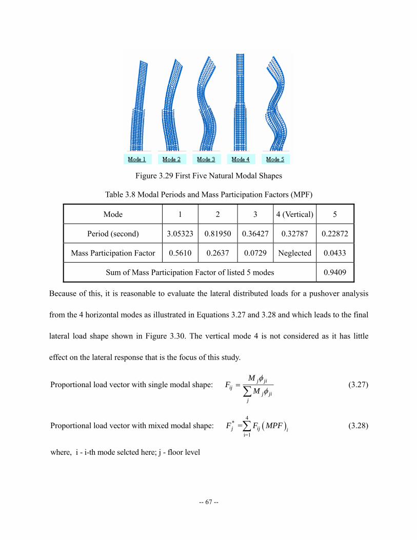
-- 67 --
Figure 3.29 First Five Natural Modal Shapes
Table 3.8 Modal Periods and Mass Participation Factors (MPF)
Mode 1 2 3 4 (Vertical) 5
Period (second) 3.05323 0.81950 0.36427 0.32787 0.22872
Mass Participation Factor 0.5610 0.2637 0.0729 Neglected 0.0433
Sum of Mass Participation Factor of listed 5 modes 0.9409
Because of this, it is reasonable to evaluate the lateral distributed loads for a pushover analysis
from the 4 horizontal modes as illustrated in Equations 3.27 and 3.28 and which leads to the final
lateral load shape shown in Figure 3.30. The vertical mode 4 is not considered as it has little
effect on the lateral response that is the focus of this study.
Proportional load vector with single modal shape: j jiij
j jij
MF
Mφφ
=∑
(3.27)
( )4
*
i=1Proportional load vector with mixed modal shape: = j ij iF F MPF∑ (3.28)
where, i - i-th mode selcted here; j - floor level
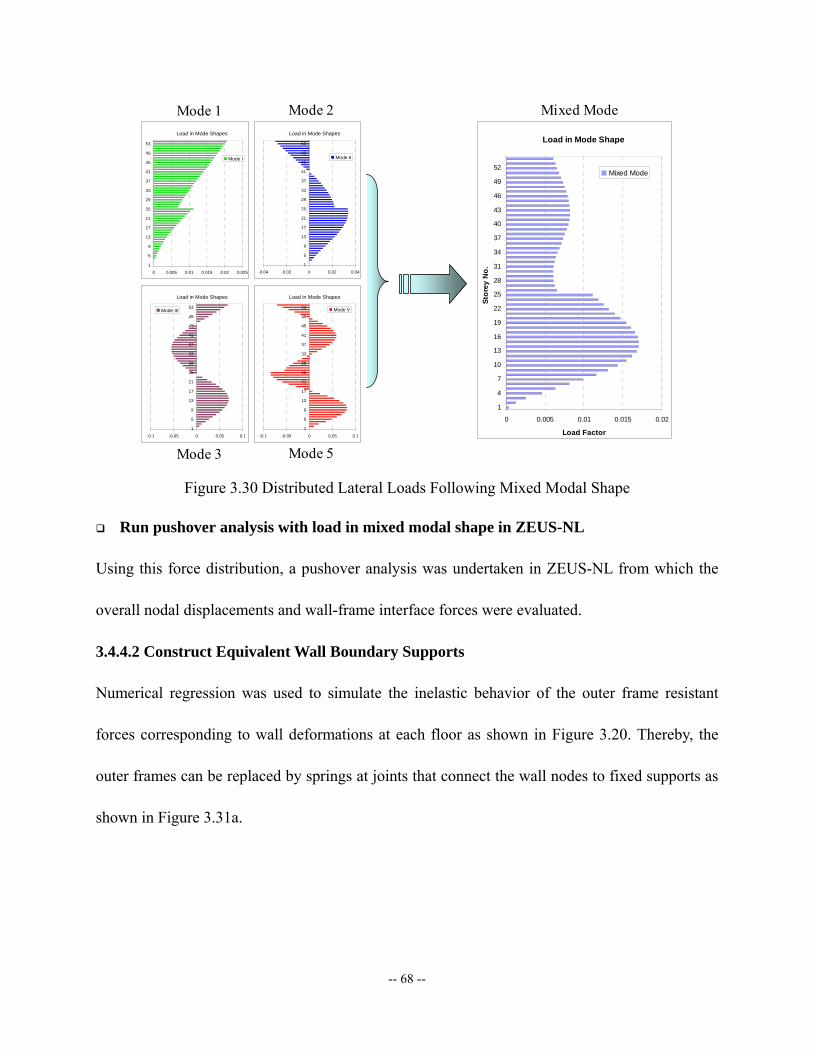
-- 68 --
Load in Mode Shapes
-0.04 -0.02 0 0.02 0.04
1
5
9
13
17
21
25
29
33
37
41
45
49
53
Mode II
Load in Mode Shapes
-0.1 -0.05 0 0.05 0.1
1
5
9
13
17
21
25
29
33
37
41
45
49
53Mode III
Load in Mode Shapes
-0.1 -0.05 0 0.05 0.1
1
5
9
13
17
21
25
29
33
37
41
45
49
53 Mode V
Load in Mode Shapes
0 0.005 0.01 0.015 0.02 0.025
1
5
9
13
17
21
25
29
33
37
41
45
49
53
Mode I
Load in Mode Shape
0 0.005 0.01 0.015 0.02
1
4
7
10
13
16
19
22
25
28
31
34
37
40
43
46
49
52
Stor
ey N
o.
Load Factor
Mixed Mode
Mode 1 Mode 2
Mode 3 Mode 5
Mixed Mode
Figure 3.30 Distributed Lateral Loads Following Mixed Modal Shape
Run pushover analysis with load in mixed modal shape in ZEUS-NL
Using this force distribution, a pushover analysis was undertaken in ZEUS-NL from which the
overall nodal displacements and wall-frame interface forces were evaluated.
3.4.4.2 Construct Equivalent Wall Boundary Supports
Numerical regression was used to simulate the inelastic behavior of the outer frame resistant
forces corresponding to wall deformations at each floor as shown in Figure 3.20. Thereby, the
outer frames can be replaced by springs at joints that connect the wall nodes to fixed supports as
shown in Figure 3.31a.
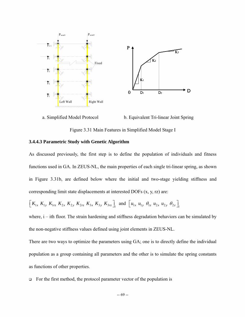
-- 69 --
Fixed
Right WallLeft Wall
Paxial2
F1
2F
F3
iF
Fi+1
axial1P
P
D
K1
K2
K3
0 D1 D2
P
D
K1
K2
K3
0 D1 D2
a. Simplified Model Protocol b. Equivalent Tri-linear Joint Spring
Figure 3.31 Main Features in Simplified Model Stage I
3.4.4.3 Parametric Study with Genetic Algorithm
As discussed previously, the first step is to define the population of individuals and fitness
functions used in GA. In ZEUS-NL, the main properties of each single tri-linear spring, as shown
in Figure 3.31b, are defined below where the initial and two-stage yielding stiffness and
corresponding limit state displacements at interested DOFs (x, y, rz) are:
1 1 1 2 2 2 3 3 3 x y rz x y rz x y rz iK K K K K K K K K⎡ ⎤⎣ ⎦ and 1 1 1 2 2 2 x y z x y z i
u u u uθ θ⎡ ⎤⎣ ⎦
where, i – ith floor. The strain hardening and stiffness degradation behaviors can be simulated by
the non-negative stiffness values defined using joint elements in ZEUS-NL.
There are two ways to optimize the parameters using GA; one is to directly define the individual
population as a group containing all parameters and the other is to simulate the spring constants
as functions of other properties.
For the first method, the protocol parameter vector of the population is
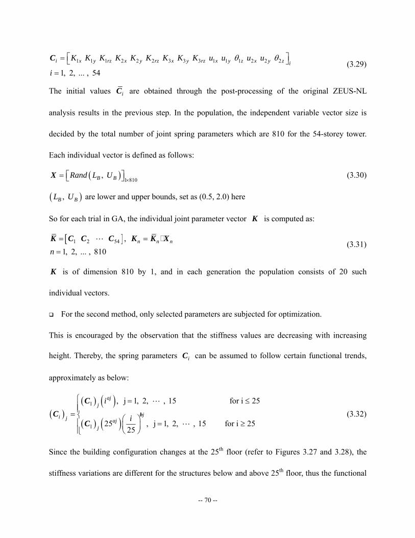
-- 70 --
1 1 1 2 2 2 3 3 3 1 1 1 2 2 2
1, 2, ... , 54
i x y rz x y rz x y rz x y z x y z i
K K K K K K K K K u u u u
i
θ θ⎡ ⎤= ⎣ ⎦=
C (3.29)
The initial values iC are obtained through the post-processing of the original ZEUS-NL
analysis results in the previous step. In the population, the independent variable vector size is
decided by the total number of joint spring parameters which are 810 for the 54-storey tower.
Each individual vector is defined as follows:
( ) 1 810, B BRand L U
×⎡ ⎤= ⎣ ⎦X (3.30)
( ), are lower and upper bounds, set as (0.5, 2.0) hereB BL U
So for each trial in GA, the individual joint parameter vector K is computed as:
[ ]1 2 54 , 1, 2, ... , 810
n n n
n= =
=
LK C C C K K X (3.31)
K is of dimension 810 by 1, and in each generation the population consists of 20 such
individual vectors.
For the second method, only selected parameters are subjected for optimization.
This is encouraged by the observation that the stiffness values are decreasing with increasing
height. Thereby, the spring parameters iC can be assumed to follow certain functional trends,
approximately as below:
( )( ) ( )
( ) ( )
1
1
, j 1, 2, , 15 for i 25
25 , j 1, 2, , 15 for i 2525
ajj
ji j ajj
i
i
⎧ = ≤⎪⎪= ⎨ ⎛ ⎞⎪ = ≥⎜ ⎟⎪ ⎝ ⎠⎩
L
Lb
CC
C (3.32)
Since the building configuration changes at the 25th floor (refer to Figures 3.27 and 3.28), the
stiffness variations are different for the structures below and above 25th floor, thus the functional
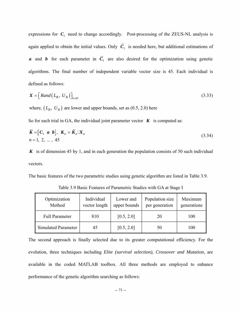
-- 71 --
expressions for iC need to change accordingly. Post-processing of the ZEUS-NL analysis is
again applied to obtain the initial values. Only 1C is needed here, but additional estimations of
a and b for each parameter in 1C are also desired for the optimization using genetic
algorithms. The final number of independent variable vector size is 45. Each individual is
defined as follows:
( ) 1 45, B BRand L U
×⎡ ⎤= ⎣ ⎦X (3.33)
( )where, , are lower and upper bounds, set as (0.5, 2.0) hereB BL U
So for each trial in GA, the individual joint parameter vector K is computed as:
[ ]1 , 1, 2, ... , 45
n n n
n= =
=
K C a b K K X (3.34)
K is of dimension 45 by 1, and in each generation the population consists of 50 such individual
vectors.
The basic features of the two parametric studies using genetic algorithm are listed in Table 3.9.
Table 3.9 Basic Features of Parametric Studies with GA at Stage I
Optimization Method
Individual vector length
Lower and upper bounds
Population size per generation
Maximum generations
Full Parameter 810 [0.5, 2.0] 20 100
Simulated Parameter 45 [0.5, 2.0] 50 100
The second approach is finally selected due to its greater computational efficiency. For the
evolution, three techniques including Elite (survival selection), Crossover and Mutation, are
available in the coded MATLAB toolbox. All three methods are employed to enhance
performance of the genetic algorithm searching as follows:

-- 72 --
Fitness function:
The main comparison between lumped model and original complete model is of the deformed
shapes under the same loadings. On account of different influences on whole building behavior
from boundary conditions at different heights, weighting factors are introduced in the
deformation based fitness function. The fitness function is defined as:
( )t oi i
oi
Fi
⎧ ⎫−⎪ ⎪= ⎨ ⎬×⎪ ⎪⎩ ⎭
D D
D (3.35)
where, Storey number = 1, 2, ..., 54
Wall nodal displacement along X at ith storey, from lumped model
Wall nodal displacement along X at ith storey, from original model
tioi
i −
−
−
D
D
Elite (selected parents with fitness values under 20% level):
1 , Generation numberi i i+ = −X X (3.36)
Crossover (two types of combinations are applied here):
Partial crossover:
(1) (1) (1) (2) (2) (2)1 1 2 1, , , (1 ) , , , i k k nnk kα α+ −⎡ ⎤= + −⎣ ⎦L LX X X X X X X (3.37)
[ ]where, Preset or random number, 0 1 , 1 , is variable vector length Generation number
k k n niα − ∈ < <
−
Complete crossover:
(1) (2)1 (1 )i i iα α+ = + −X X X (3.38)
[ ]where, preset value or random number, 0 1 ; Generation numberiα − ∈ −
Mutation (scale or shrink according to the fitness performance level):
( ) ( ) ( )1 , 1, 2, ... , 45i i in n n n+ = =X X β (3.39)
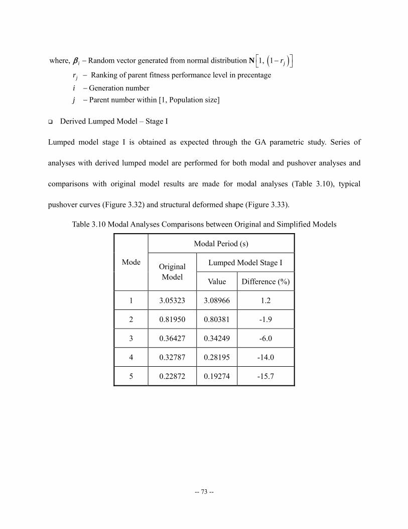
-- 73 --
( )where, Random vector generated from normal distribution 1, 1
Ranking of parent fitness performance level in precentage
Generation number Pare
Ni j
j
r
r
ij
⎡ ⎤− −⎣ ⎦−
−−
β
nt number within [1, Population size]
Derived Lumped Model – Stage I
Lumped model stage I is obtained as expected through the GA parametric study. Series of
analyses with derived lumped model are performed for both modal and pushover analyses and
comparisons with original model results are made for modal analyses (Table 3.10), typical
pushover curves (Figure 3.32) and structural deformed shape (Figure 3.33).
Table 3.10 Modal Analyses Comparisons between Original and Simplified Models
Modal Period (s)
Lumped Model Stage I Mode Original Model Value Difference (%)
1 3.05323 3.08966 1.2
2 0.81950 0.80381 -1.9
3 0.36427 0.34249 -6.0
4 0.32787 0.28195 -14.0
5 0.22872 0.19274 -15.7
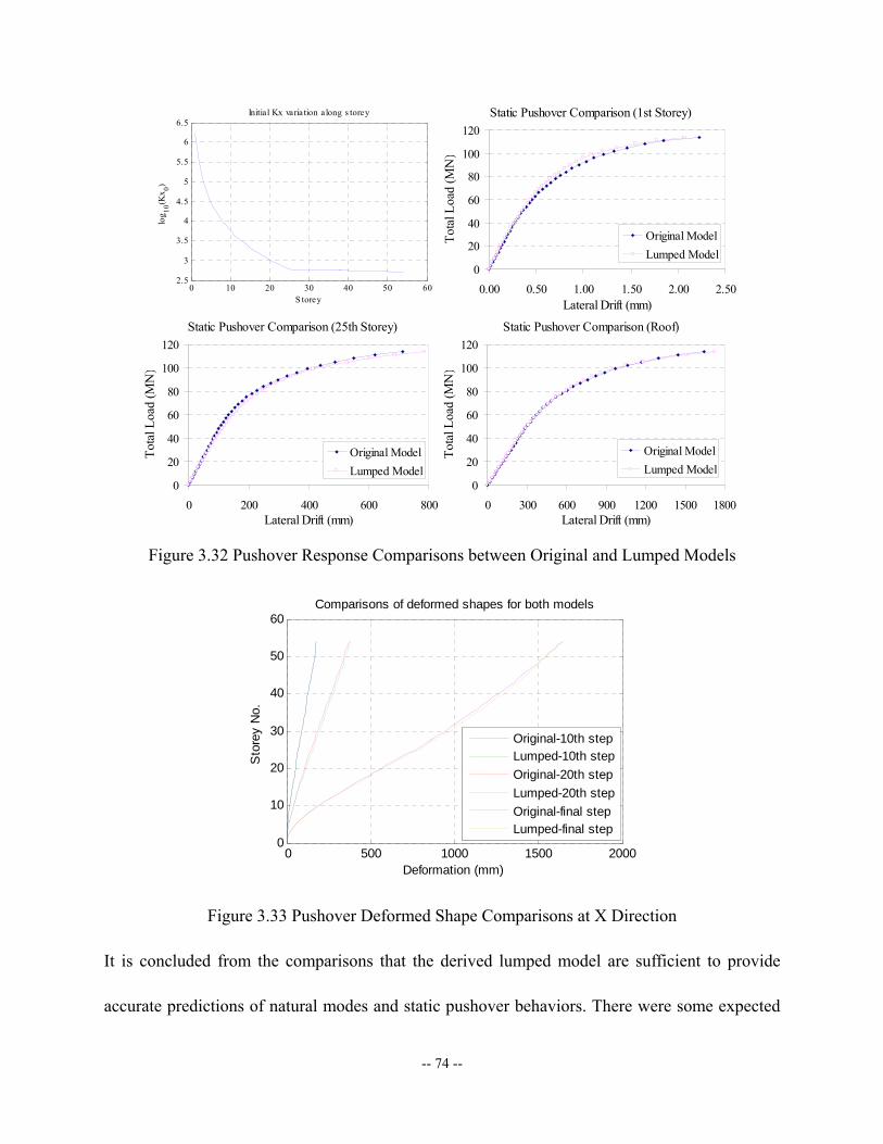
-- 74 --
0 10 20 30 40 50 602.5
3
3.5
4
4.5
5
5.5
6
6.5
S torey
log 10
(Kx 0)
Initial Kx variation along s torey Static Pushover Comparison (1st Storey)
0
20
40
60
80
100
120
0.00 0.50 1.00 1.50 2.00 2.50Lateral Drift (mm)
Tota
l Loa
d (M
N)
Original ModelLumped Model
Static Pushover Comparison (25th Storey)
0
20
40
60
80
100
120
0 200 400 600 800Lateral Drift (mm)
Tota
l Loa
d (M
N)
Original ModelLumped Model
Static Pushover Comparison (Roof)
0
20
40
60
80
100
120
0 300 600 900 1200 1500 1800Lateral Drift (mm)
Tota
l Loa
d (M
N)
Original ModelLumped Model
Figure 3.32 Pushover Response Comparisons between Original and Lumped Models
0 500 1000 1500 20000
10
20
30
40
50
60
Deformation (mm)
Sto
rey
No.
Comparisons of deformed shapes for both models
Original-10th stepLumped-10th stepOriginal-20th stepLumped-20th stepOriginal-final stepLumped-final step
Figure 3.33 Pushover Deformed Shape Comparisons at X Direction
It is concluded from the comparisons that the derived lumped model are sufficient to provide
accurate predictions of natural modes and static pushover behaviors. There were some expected

-- 75 --
errors including shorter periods for higher modes and larger resistant forces in the highly
inelastic range. The explanation for these errors may lie in the computational joint models used
in ZEUS-NL that require non-negative tangent stiffness values and thereby make it difficult to
detect actual strain softening of the substitute outer frame. Hence, the lumped model is a little
stiffer than the complete frame model in some cases, especially for higher modes and large
deformation ranges where the RC outer frame members are more likely to get damaged. Such
errors may be taking into consideration by slight adjustments in uncertainties.
Similar comparisons were also made using DRHA as shown in Figure 3.34b ~ c; the sample
ground motion record from Kocaeli Earthquake (1999, Turkey, Duzce station) is given in Figure
3.34a.
At intermediate and top height levels, relative displacement time histories from the lumped
model are quite close to those from the original model. That means that the lumped model well
replicates the predicted seismic behavior of the selected building.

-- 76 --
a. Strong motion
Time [sec]54.543.532.521.510.50
Acc
eler
atio
n [g
]
0.30.20.1
0-0.1-0.2-0.3
b. 25th Floor Comparison between Models (Drift at 25th Floor)
-20
-15
-10
-5
0
5
10
15
20
0 1 2 3 4 5 6
Time (sec)
Late
ral D
rift (
mm
)
Original ModelLumped Model
c. Roof Comparison between Models (Top drift)
-50
-40
-30
-20
-10
0
10
20
30
40
0 1 2 3 4 5 6
Time (sec)
Late
rla D
rift (
mm
)
Original ModelLumped Model
Figure 3.34 Dynamic Response History Comparisons between Original and Lumped Models
3.4.5 Simplification Stage II Using Genetic Algorithm
3.4.5.1 VecTor2 Analysis Using Continuum FEM Model
The objective of this simplification is to produce a simple lumped-parameter model that will
provide a similar prediction of the pushover response as that which would be predicted from a
2D continuum analysis for the core wall panels. The program VecTor2 is used to provide the

-- 77 --
continuum analysis predictions. Both the SVLEM and MVLEM models, described in Figures
3.16 and 3.17, are considered for developing the lumped model in ZEUS-NL. The GA process is
employed for parameter value selection. In addition, the “hsv” type joint is applied to consider
the axial load-shear interaction effects in ZEUS-NL (Lee and Elnashai (2002)). For all wall
panels of the same size, only one parametric study for lumped modeling is required. The core
wall panel is modeled as shown in Figure 3.35a~c.
3.4
m
L = 9.33 ~ 9.43 m
F1
axialP
Mtop
B=1
.575
0.325
0.45
0.325
axial
1p (kN/node)
v2p (by M , kN/node)
p (by P , kN/node)v1
top
a. Wall Prototype b. Equivalent Nodal Loads c. FEM Model in VecTor2
Figure 3.35 Discrete FEM Model of Core Wall Panel
In the VecTor2 pushover analyses, the axial loads at different levels as shown in Table 3.11 are
imposed as initial load corresponding for the different analyses as required by the nonlinear hsv
joints in ZEUS-NL. Horizontal loads are incrementally applied in displacement control. All loads
are equivalent to uniformly distributed nodal loads along the floor at the top of wall panel.
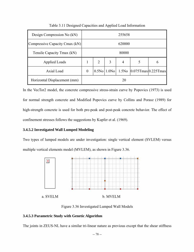
-- 78 --
Table 3.11 Designed Capacities and Applied Load Information
Design Compression No (kN) 255658
Compressive Capacity Cmax (kN) 620000
Tensile Capacity Tmax (kN) 80000
Applied Loads 1 2 3 4 5 6
Axial Load 0 0.5No 1.0No 1.5No 0.075Tmax 0.225Tmax
Horizontal Displacement (mm) 20
In the VecTor2 model, the concrete compressive stress-strain curve by Popovics (1973) is used
for normal strength concrete and Modified Popovics curve by Collins and Porasz (1989) for
high-strength concrete is used for both pre-peak and post-peak concrete behavior. The effect of
confinement stresses follows the suggestions by Kupfer et al. (1969).
3.4.5.2 Investigated Wall Lumped Modeling
Two types of lumped models are under investigation: single vertical element (SVLEM) versus
multiple vertical elements model (MVLEM), as shown in Figure 3.36.
a. SVELM b. MVELM
Figure 3.36 Investigated Lumped Wall Models
3.4.5.3 Parametric Study with Genetic Algorithm
The joints in ZEUS-NL have a similar tri-linear nature as previous except that the shear stiffness
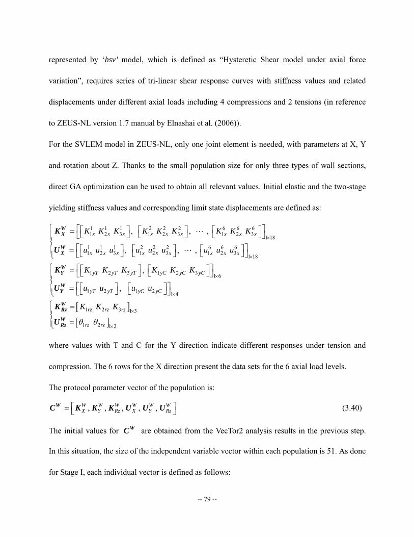
-- 79 --
represented by ‘hsv’ model, which is defined as “Hysteretic Shear model under axial force
variation”, requires series of tri-linear shear response curves with stiffness values and related
displacements under different axial loads including 4 compressions and 2 tensions (in reference
to ZEUS-NL version 1.7 manual by Elnashai et al. (2006)).
For the SVLEM model in ZEUS-NL, only one joint element is needed, with parameters at X, Y
and rotation about Z. Thanks to the small population size for only three types of wall sections,
direct GA optimization can be used to obtain all relevant values. Initial elastic and the two-stage
yielding stiffness values and corresponding limit state displacements are defined as:
1 1 1 2 2 2 6 6 61 2 3 1 2 3 1 2 3 1 18
1 1 1 2 2 2 6 6 61 2 3 1 2 3 1 2 3 1 18
1 2 3 1 2 3
, , ,
, , ,
,
x x x x x x x x x
x x x x x x x x x
yT yT yT yC yC yC
K K K K K K K K K
u u u u u u u u u
K K K K K K
×
×
⎧ ⎡ ⎤⎡ ⎤ ⎡ ⎤ ⎡ ⎤= ⎣ ⎦ ⎣ ⎦ ⎣ ⎦⎣ ⎦⎪⎨
⎡ ⎤⎡ ⎤ ⎡ ⎤ ⎡ ⎤=⎪ ⎣ ⎦ ⎣ ⎦ ⎣ ⎦⎣ ⎦⎩
⎡ ⎤ ⎡ ⎤= ⎣ ⎦ ⎣
L
L
WX
WX
WY
K
U
K
[ ][ ]
1 6
1 2 1 2 1 4
1 2 3 1 3
1 2 1 2
,
yT yT yC yC
rz rz rz
rz rz
u u u u
K K K
θ θ
×
×
×
×
⎧ ⎡ ⎤⎦⎣ ⎦⎪⎨
⎡ ⎤⎡ ⎤ ⎡ ⎤=⎪ ⎣ ⎦ ⎣ ⎦⎣ ⎦⎩⎧ =⎪⎨
=⎪⎩
WY
WRz
WRz
U
K
U
where values with T and C for the Y direction indicate different responses under tension and
compression. The 6 rows for the X direction present the data sets for the 6 axial load levels.
The protocol parameter vector of the population is:
, , , , , W W W W W WX Y Rz X Y Rz⎡ ⎤= ⎣ ⎦
WC K K K U U U (3.40)
The initial values for WC are obtained from the VecTor2 analysis results in the previous step.
In this situation, the size of the independent variable vector within each population is 51. As done
for Stage I, each individual vector is defined as follows:
-- 80 --
( ) 1 51, B BRand L U
×⎡ ⎤= ⎣ ⎦
WX (3.41)
( ), are lower and upper bounds, set as (0.5, 2.0) hereB BL U
So for each trial in GA, the individual joint parameter vector K is computed as:
1, 2, ... , 51n n n
n=
=
W WK C X (3.42)
A similar procedure is applied for MVLEM model, except now for a total of five joint elements
including four vertical springs at the bottom and one horizontal spring at the lower part of the
wall panel. The basic features of the two parametric studies using GA are listed in Table 3.12.
Table 3.12 Basic Features of Parametric Studies with GA at Stage II
Model Individual vector length
Lower and upper bounds
Population size per generation
Maximum generations
SVLEM 51 [0.5, 2.0] 50 100
MVLEM 66 [0.5, 2.0] 50 100
As in Stage I, the three techniques of Elite (survival selection), Crossover and Mutation, are
employed for generating populations using the genetic algorithm toolbox, as described by
Equations 3.36~3.39. In the ZEUS analysis for fragility assessment, nodal displacements at the
center of wall panel at each floor level are required. Therefore, the main comparison between the
optimized lumped model and the RC continuum model were control point displacements.
Because the floor slab is treated as rigid in the ZEUS-NL model, while not in VecTor2, the nodal
rotation at control points is excluded from the comparisons. It follows that the fitness function is
defined as:
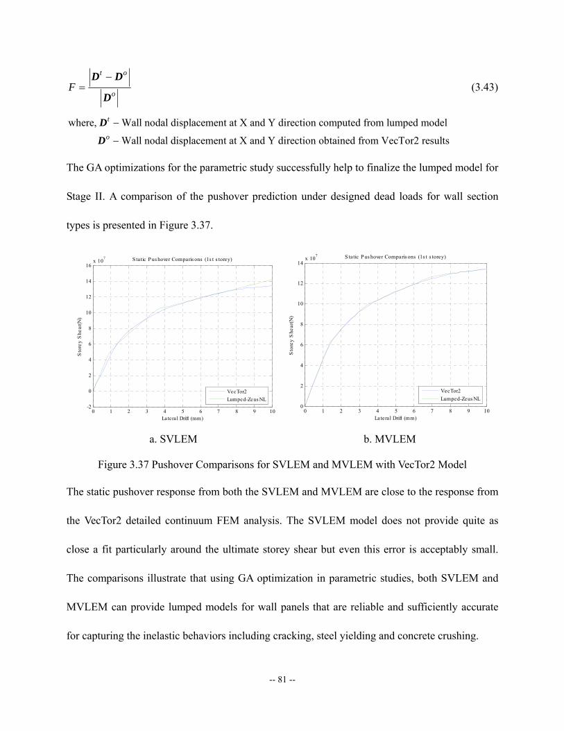
-- 81 --
t o
oF
−=
D D
D (3.43)
where, Wall nodal displacement at X and Y direction computed from lumped model
Wall nodal displacement at X and Y direction obtained from VecTor2 results
t
o
−
−
D
D
The GA optimizations for the parametric study successfully help to finalize the lumped model for
Stage II. A comparison of the pushover prediction under designed dead loads for wall section
types is presented in Figure 3.37.
0 1 2 3 4 5 6 7 8 9 10-2
0
2
4
6
8
10
12
14
16x 10
7
Lateral Drift (mm)
Sto
rey
She
ar(N
)
S tatic P us hover Comparis ons (1s t s torey)
VecTor2Lumped-Zeus NL
0 1 2 3 4 5 6 7 8 9 100
2
4
6
8
10
12
14x 107
Lateral Drift (mm)
Sto
rey
She
ar(N
)
S tatic P us hover Comparis ons (1s t s torey)
VecTor2Lumped-Zeus NL
a. SVLEM b. MVLEM
Figure 3.37 Pushover Comparisons for SVLEM and MVLEM with VecTor2 Model
The static pushover response from both the SVLEM and MVLEM are close to the response from
the VecTor2 detailed continuum FEM analysis. The SVLEM model does not provide quite as
close a fit particularly around the ultimate storey shear but even this error is acceptably small.
The comparisons illustrate that using GA optimization in parametric studies, both SVLEM and
MVLEM can provide lumped models for wall panels that are reliable and sufficiently accurate
for capturing the inelastic behaviors including cracking, steel yielding and concrete crushing.
-- 82 --
3.4.6 Lumped Model Evaluation
Through the implementation of the above two-stage model optimization procedure, a
comparatively simple lumped-parameter model is created that consists of beam elements, rigid
bars, and nonlinear springs. The simplified model is sufficiently accurate for evaluating nodal
displacements, global internal forces, and at the same time accounting for shear deformations
within the structural walls. The required computational time for completing a DRHA is reduced
to a small fraction of what it would have been for an analysis of the original model. Table 3.13
compares the details and computational times between the original whole building frame model
and the final lumped model in ZEUS-NL. Though it took around one week to actually complete
the lumped modeling process for this specific building, the computational saving of next step
DRHA runtime is much more significant compared to this cost. The total estimated runtime of
DRHA and post-process for the reference structure is about 3 hours per 1000 time steps which
leads to 1800 hours (2.5 months) when considering a total of 600 ground motion records with
average 1000 time steps. So the time can be reduced to less than 180 hours (1 week) when using
derived lumped model, which creates more research flexibility for making fragility assessments.
In addition, the methodology developed in this research can be extended and applied to other
complex structures.
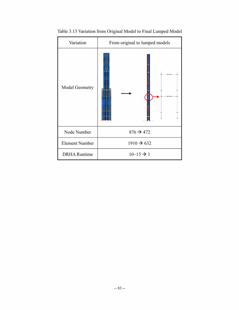
-- 83 --
Table 3.13 Variation from Original Model to Final Lumped Model
Variation From original to lumped models
Model Geometry
Node Number 876 472
Element Number 1910 632
DRHA Runtime 10~15 1
-- 84 --
4. Limit States Definition
4.1 Literature Survey
4.1.1 Overview
The definition of limit states plays a significant role in the construction of the fragility curves due
to its direct effect on evaluation of building performance levels. The analytical fragility
assessment requires the appropriate and easily tracked damage scales for the evaluation of the
system demand and capacity. There are two ways to characterize the performance level or limit
states: qualitative and quantitative approaches.
Qualitative Approach
These kinds of approaches have traditionally been used in building codes. FEMA273 (1997) and
its update FEMA 356, has very comprehensive documentation on performance levels that are
defined qualitatively and is briefly summarized in Table 4.1. Rossetto and Elnashai (2003)
defined seven limit states for derivation of fragility curve based on observational data, and
employed a creative damage index so-called the homogenized damage scale for reinforced
concrete buildings (HRC-Scale) for the performance level representation from 0 for no damage
to 100 for collapse, as shown in Table 4.2, in terms of the typical structural and non-structural
damage for the four main types of reinforced concrete structures found in Europe, (i.e. ductile
and non-ductile frames, frames with masonry infill and shear-wall structures). Because of the
lack of researches for RC high-rise buildings, especially of structural wall systems, current
qualitative approaches can only serve as references.
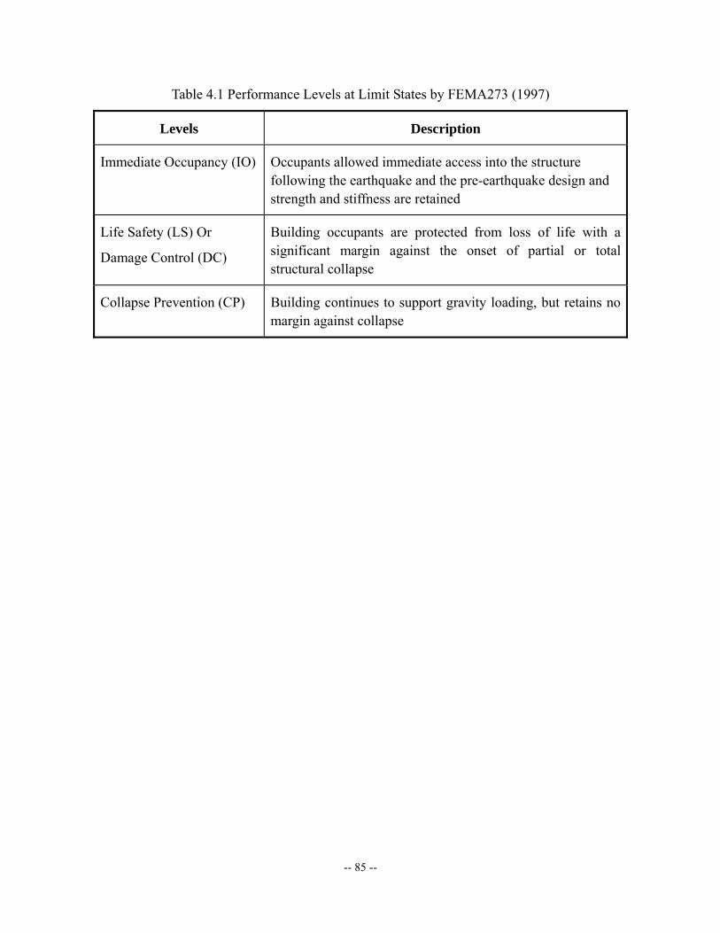
-- 85 --
Table 4.1 Performance Levels at Limit States by FEMA273 (1997)
Levels Description
Immediate Occupancy (IO) Occupants allowed immediate access into the structure following the earthquake and the pre-earthquake design and strength and stiffness are retained
Life Safety (LS) Or
Damage Control (DC)
Building occupants are protected from loss of life with a significant margin against the onset of partial or total structural collapse
Collapse Prevention (CP) Building continues to support gravity loading, but retains no margin against collapse
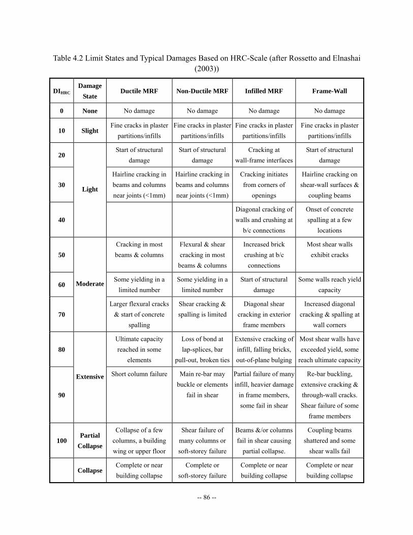
-- 86 --
Table 4.2 Limit States and Typical Damages Based on HRC-Scale (after Rossetto and Elnashai (2003))
DIHRC Damage
State Ductile MRF Non-Ductile MRF Infilled MRF Frame-Wall
0 None No damage No damage No damage No damage
10 Slight Fine cracks in plaster
partitions/infills Fine cracks in plaster
partitions/infills Fine cracks in plaster
partitions/infills Fine cracks in plaster
partitions/infills
20 Start of structural
damage Start of structural
damage Cracking at
wall-frame interfaces Start of structural
damage
30 Hairline cracking in beams and columns near joints (<1mm)
Hairline cracking in beams and columns near joints (<1mm)
Cracking initiates from corners of
openings
Hairline cracking on shear-wall surfaces &
coupling beams
40
Light
Diagonal cracking of walls and crushing at
b/c connections
Onset of concrete spalling at a few
locations
50 Cracking in most beams & columns
Flexural & shear cracking in most
beams & columns
Increased brick crushing at b/c
connections
Most shear walls exhibit cracks
60 Some yielding in a
limited number Some yielding in a
limited number Start of structural
damage Some walls reach yield
capacity
70
Moderate
Larger flexural cracks & start of concrete
spalling
Shear cracking & spalling is limited
Diagonal shear cracking in exterior
frame members
Increased diagonal cracking & spalling at
wall corners
80 Ultimate capacity reached in some
elements
Loss of bond at lap-splices, bar
pull-out, broken ties
Extensive cracking of infill, falling bricks, out-of-plane bulging
Most shear walls have exceeded yield, some
reach ultimate capacity
90
Extensive Short column failure Main re-bar may buckle or elements
fail in shear
Partial failure of many infill, heavier damage
in frame members, some fail in shear
Re-bar buckling, extensive cracking & through-wall cracks. Shear failure of some
frame members
100 Partial
Collapse
Collapse of a few columns, a building wing or upper floor
Shear failure of many columns or soft-storey failure
Beams &/or columns fail in shear causing
partial collapse.
Coupling beams shattered and some
shear walls fail
Collapse Complete or near building collapse
Complete or soft-storey failure
Complete or near building collapse
Complete or near building collapse
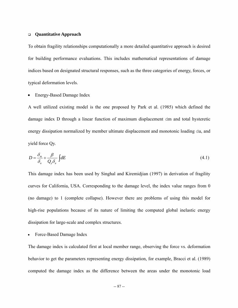
-- 87 --
Quantitative Approach
To obtain fragility relationships computationally a more detailed quantitative approach is desired
for building performance evaluations. This includes mathematical representations of damage
indices based on designated structural responses, such as the three categories of energy, forces, or
typical deformation levels.
• Energy-Based Damage Index
A well utilized existing model is the one proposed by Park et al. (1985) which defined the
damage index D through a linear function of maximum displacement dm and total hysteretic
energy dissipation normalized by member ultimate displacement and monotonic loading du, and
yield force Qy.
m
u y u
D dEQ
δ βδ δ
= + ∫ (4.1)
This damage index has been used by Singhal and Kiremidjian (1997) in derivation of fragility
curves for California, USA. Corresponding to the damage level, the index value ranges from 0
(no damage) to 1 (complete collapse). However there are problems of using this model for
high-rise populations because of its nature of limiting the computed global inelastic energy
dissipation for large-scale and complex structures.
• Force-Based Damage Index
The damage index is calculated first at local member range, observing the force vs. deformation
behavior to get the parameters representing energy dissipation, for example, Bracci et al. (1989)
computed the damage index as the difference between the areas under the monotonic load
-- 88 --
response and the cyclic load response envelope curves. The global damage can be found using
similar method as Park et al. (1985). The problem for these kinds of indices is that the load
response behavior and the damage index calculation are mainly based on some selected
predominant modes, which is not adequate for high-rise buildings that have complicated
vibration modes and hence it is very difficult to obtain appropriate index value from the energy
dissipation investigation.
• Deformation-Based Damage Index
Compared with the previous two, this type is more intuitive, straightforward, comprehensive and
easier for calibration with investigation or experimental data, because these measures are
sufficient to show the detailed structural behavior under seismic loads, not only including global
displacements, but also local damage including cracking and yielding mechanisms. This fits the
characteristics of the response of RC high-rise buildings quite well.
Generally, the response parameter mostly used in storey level is the maximum inter-storey drift
ratio (ISD) since it is easily to relate to the structural damage and inelastic behavior. But for RC
high-rise buildings, it is still necessary to be able to track the global performance. So also global
drift ratio is important in this study. Many researchers and institutes have employed the lateral
drift ratios for the damage evaluation of structures, such as FEMA273 (1997), Kircher et al.
(1997), Mosalem et al. (1997), etc.). Jeong and Elnashai (2004a) have proposed a 3D damage
index for irregular RC frame structures counting more complete concerns and influencing factors
in spatial building behavior.
Usually the limit states can be detected through sets of pushover analyses for the prototype
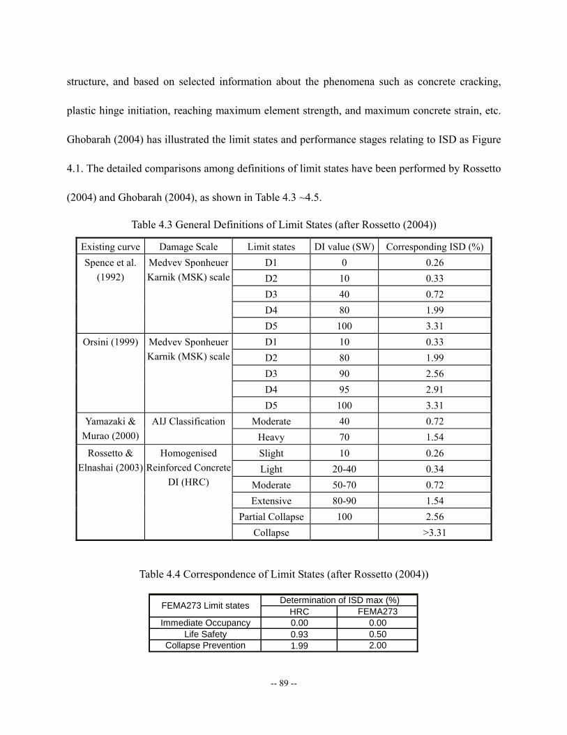
-- 89 --
structure, and based on selected information about the phenomena such as concrete cracking,
plastic hinge initiation, reaching maximum element strength, and maximum concrete strain, etc.
Ghobarah (2004) has illustrated the limit states and performance stages relating to ISD as Figure
4.1. The detailed comparisons among definitions of limit states have been performed by Rossetto
(2004) and Ghobarah (2004), as shown in Table 4.3 ~4.5.
Table 4.3 General Definitions of Limit States (after Rossetto (2004))
Existing curve Damage Scale Limit states DI value (SW) Corresponding ISD (%) D1 0 0.26 D2 10 0.33 D3 40 0.72 D4 80 1.99
Spence et al. (1992)
Medvev Sponheuer Karnik (MSK) scale
D5 100 3.31 D1 10 0.33 D2 80 1.99 D3 90 2.56 D4 95 2.91
Orsini (1999) Medvev Sponheuer Karnik (MSK) scale
D5 100 3.31 Moderate 40 0.72 Yamazaki &
Murao (2000) AIJ Classification
Heavy 70 1.54 Slight 10 0.26 Light 20-40 0.34
Moderate 50-70 0.72 Extensive 80-90 1.54
Partial Collapse 100 2.56
Rossetto & Elnashai (2003)
Homogenised Reinforced Concrete
DI (HRC)
Collapse >3.31
Table 4.4 Correspondence of Limit States (after Rossetto (2004))
HRC FEMA273Immediate Occupancy 0.00 0.00
Life Safety 0.93 0.50Collapse Prevention 1.99 2.00
Determination of ISD max (%)FEMA273 Limit states
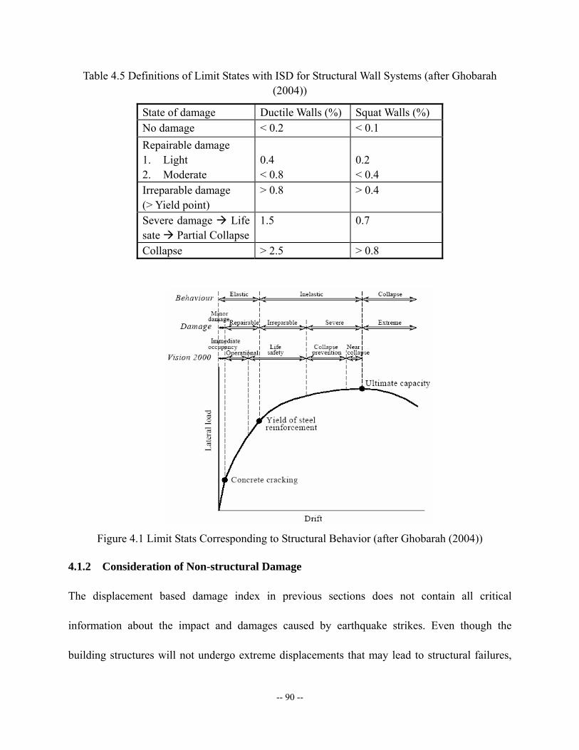
-- 90 --
Table 4.5 Definitions of Limit States with ISD for Structural Wall Systems (after Ghobarah (2004))
State of damage Ductile Walls (%) Squat Walls (%) No damage < 0.2 < 0.1 Repairable damage 1. Light 2. Moderate
0.4 < 0.8
0.2 < 0.4
Irreparable damage (> Yield point)
> 0.8 > 0.4
Severe damage Life sate Partial Collapse
1.5 0.7
Collapse > 2.5 > 0.8
Figure 4.1 Limit Stats Corresponding to Structural Behavior (after Ghobarah (2004))
4.1.2 Consideration of Non-structural Damage
The displacement based damage index in previous sections does not contain all critical
information about the impact and damages caused by earthquake strikes. Even though the
building structures will not undergo extreme displacements that may lead to structural failures,

-- 91 --
the interior or attached non-structural facilities may still be damaged severely and great losses
can be expected since most high-rise buildings are either commercial or residential centers.
Non-structural components are defined for those attachments or facilities within the building
with purposes for either functionalities or decorations, as illuminated in Figure 4.2.
Figure 4.2 Typical Non-structural Components in Building (from WJE (1994))
Ordinary non-structural components include two categories:
• Architectural components. Including ceiling, cladding, exterior and interior non-bearing infill
and partitions, furniture and equipments, and other decorations
• Mechanical and electrical components. Containing storage, water and gas piping systems,
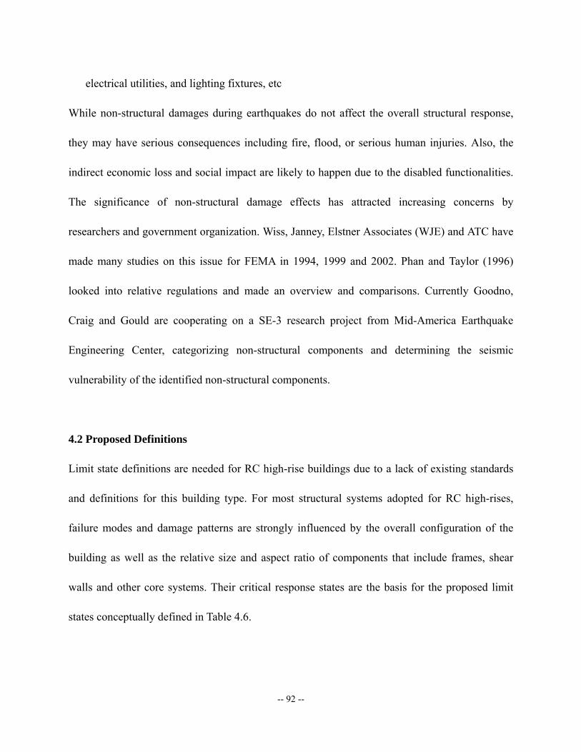
-- 92 --
electrical utilities, and lighting fixtures, etc
While non-structural damages during earthquakes do not affect the overall structural response,
they may have serious consequences including fire, flood, or serious human injuries. Also, the
indirect economic loss and social impact are likely to happen due to the disabled functionalities.
The significance of non-structural damage effects has attracted increasing concerns by
researchers and government organization. Wiss, Janney, Elstner Associates (WJE) and ATC have
made many studies on this issue for FEMA in 1994, 1999 and 2002. Phan and Taylor (1996)
looked into relative regulations and made an overview and comparisons. Currently Goodno,
Craig and Gould are cooperating on a SE-3 research project from Mid-America Earthquake
Engineering Center, categorizing non-structural components and determining the seismic
vulnerability of the identified non-structural components.
4.2 Proposed Definitions
Limit state definitions are needed for RC high-rise buildings due to a lack of existing standards
and definitions for this building type. For most structural systems adopted for RC high-rises,
failure modes and damage patterns are strongly influenced by the overall configuration of the
building as well as the relative size and aspect ratio of components that include frames, shear
walls and other core systems. Their critical response states are the basis for the proposed limit
states conceptually defined in Table 4.6.
-- 93 --
Table 4.6 Definitions of Limit States
Level Limit State Description
Limit State 1 (LS1) Serviceability Determined at minor cracks point of main resisting members like core wall here
Limit State 2 (LS2) Damage Control First yielding of longitudinal steel reinforcement, or presence of first plastic hinge (may only apply for beam or columns)
Limit State 3 (LS3) Collapse Prevention Ultimate point of main resisting members and starting point of decreasing of overall capacity curve
The associated quantitative criteria for these definitions are derived from the results of pushover
analyses are presented hereafter. The combination of overall load-displacement relationships and
local damage patterns will help to determine the critical structural behavior stages.
4.2.1 Global Pushover Analysis with Whole Frame Model
To obtain the global response of the building, pushover analysis of the entire structure is
necessary. Full fiber-based model of whole structure is constructed in ZEUS-NL. The
combination of the first 4 natural modal shapes, weighted by modal mass participation factors, is
used for the lateral load distribution pattern. By the approach, the overall load-displacement
relationships could be assessed, figuring out the critical structural behavior stages by considering
two methods:
• The evaluation of yielding and ultimate deformation quantities from pushover curve can be
achieved through several ways by finding equivalent bi-linear response curves proposed by
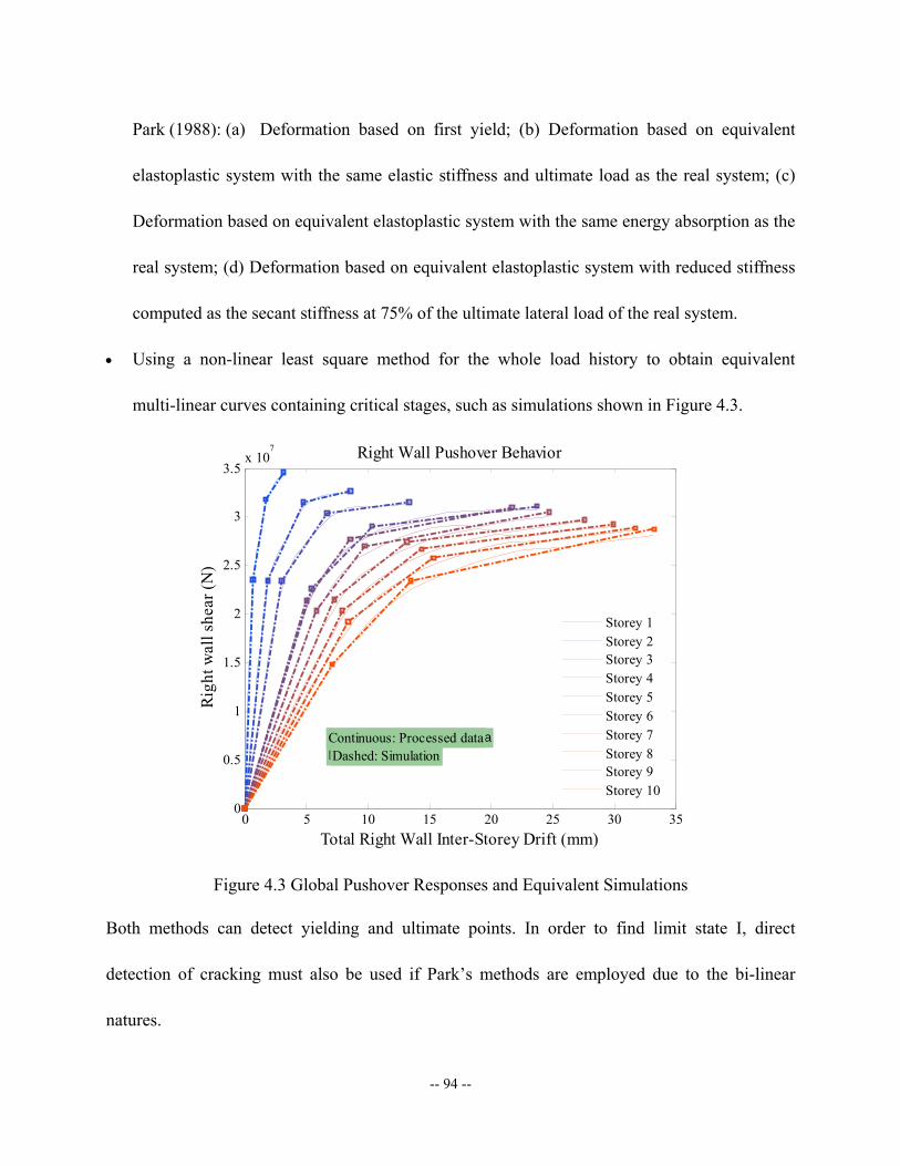
-- 94 --
Park (1988): (a) Deformation based on first yield; (b) Deformation based on equivalent
elastoplastic system with the same elastic stiffness and ultimate load as the real system; (c)
Deformation based on equivalent elastoplastic system with the same energy absorption as the
real system; (d) Deformation based on equivalent elastoplastic system with reduced stiffness
computed as the secant stiffness at 75% of the ultimate lateral load of the real system.
• Using a non-linear least square method for the whole load history to obtain equivalent
multi-linear curves containing critical stages, such as simulations shown in Figure 4.3.
0 5 10 15 20 25 30 350
0.5
1
1.5
2
2.5
3
3.5x 10
7
Total Right Wall Inter-Storey Drift (mm)
Righ
t wal
l she
ar (N
)
Right Wall Pushover Behavior
Continuous: Processed dataDashed: SimulationContinuous: Processed dataDashed: Simulation
Storey 1Storey 2Storey 3Storey 4Storey 5Storey 6Storey 7Storey 8Storey 9Storey 10
Figure 4.3 Global Pushover Responses and Equivalent Simulations
Both methods can detect yielding and ultimate points. In order to find limit state I, direct
detection of cracking must also be used if Park’s methods are employed due to the bi-linear
natures.
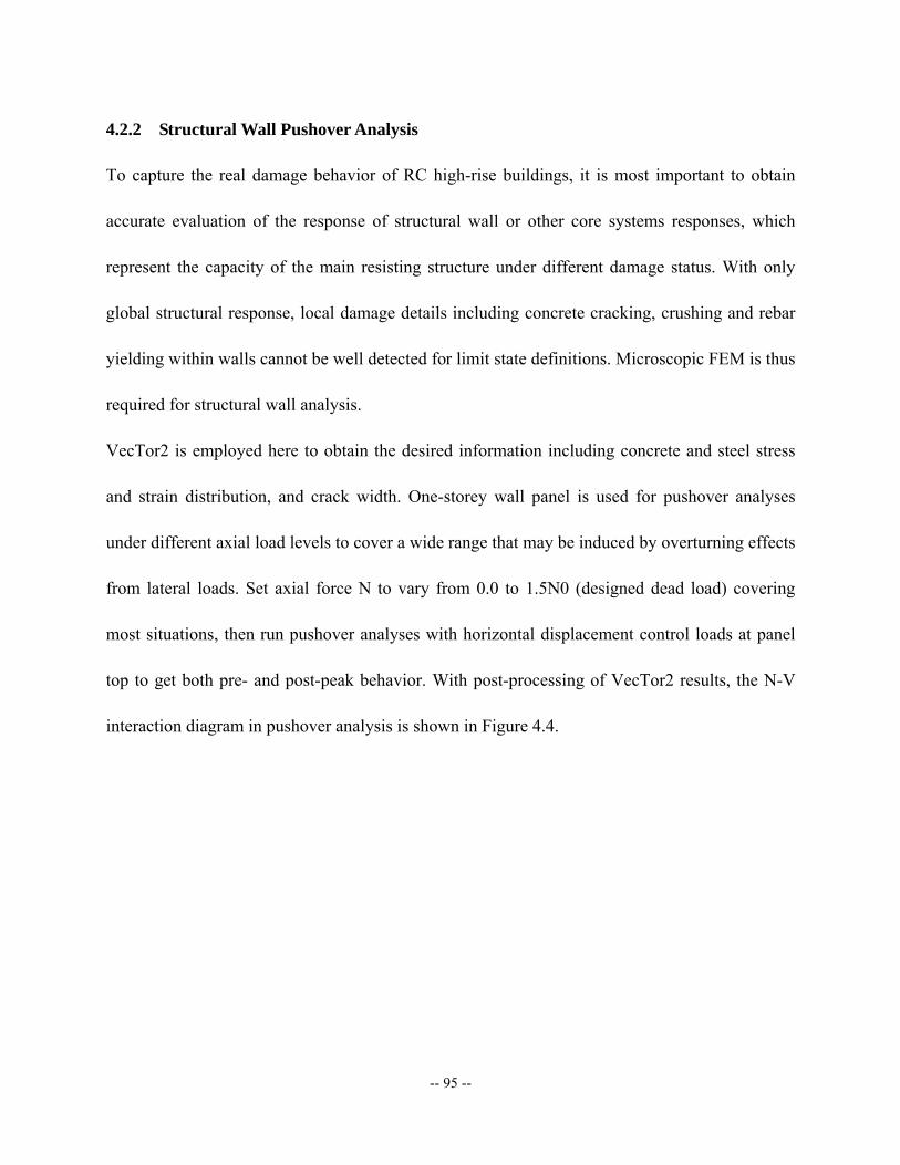
-- 95 --
4.2.2 Structural Wall Pushover Analysis
To capture the real damage behavior of RC high-rise buildings, it is most important to obtain
accurate evaluation of the response of structural wall or other core systems responses, which
represent the capacity of the main resisting structure under different damage status. With only
global structural response, local damage details including concrete cracking, crushing and rebar
yielding within walls cannot be well detected for limit state definitions. Microscopic FEM is thus
required for structural wall analysis.
VecTor2 is employed here to obtain the desired information including concrete and steel stress
and strain distribution, and crack width. One-storey wall panel is used for pushover analyses
under different axial load levels to cover a wide range that may be induced by overturning effects
from lateral loads. Set axial force N to vary from 0.0 to 1.5N0 (designed dead load) covering
most situations, then run pushover analyses with horizontal displacement control loads at panel
top to get both pre- and post-peak behavior. With post-processing of VecTor2 results, the N-V
interaction diagram in pushover analysis is shown in Figure 4.4.
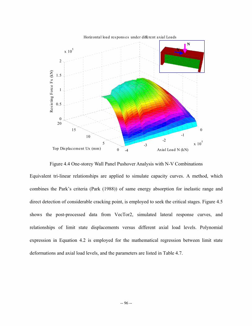
-- 96 --
-4-3
-2-1
0
x 105
05
10
1520
0
0.5
1
1.5
2
x 105
Axial Load N (kN)
Horizontal load res pons es under different axial Loads
Top Dis placement Ux (mm)
Res
istin
g Fo
rce
Fx (k
N)
Figure 4.4 One-storey Wall Panel Pushover Analysis with N-V Combinations
Equivalent tri-linear relationships are applied to simulate capacity curves. A method, which
combines the Park’s criteria (Park (1988)) of same energy absorption for inelastic range and
direct detection of considerable cracking point, is employed to seek the critical stages. Figure 4.5
shows the post-processed data from VecTor2, simulated lateral response curves, and
relationships of limit state displacements versus different axial load levels. Polynomial
expression in Equation 4.2 is employed for the mathematical regression between limit state
deformations and axial load levels, and the parameters are listed in Table 4.7.
NV
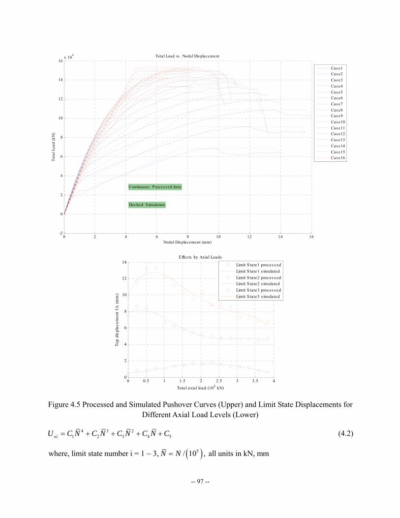
-- 97 --
0 2 4 6 8 10 12 14 16-2
0
2
4
6
8
10
12
14
16x 10
4
Nodal Dis placement (mm)
Tota
l Loa
d (k
N)
Total Load vs . Nodal Dis placement
Continuous : P roces s ed data
Das hed: S imulation
Cas e1Cas e2Cas e3Cas e4Cas e5Cas e6Cas e7Cas e8Cas e9Cas e10Cas e11Cas e12Cas e13Cas e14Cas e15Cas e16
0 0.5 1 1.5 2 2.5 3 3.5 40
2
4
6
8
10
12
14
Total axial load (105 kN)
Top
disp
lace
men
t Ux
(mm
)
Effects by Axial Loads
Limit S tate1 proces s edLimit S tate1 s imulatedLimit S tate2 proces s edLimit S tate2 s imulatedLimit S tate3 proces s edLimit S tate3 s imulated
Figure 4.5 Processed and Simulated Pushover Curves (Upper) and Limit State Displacements for Different Axial Load Levels (Lower)
4 3 21 2 3 4 5xiU C N C N C N C N C= + + + + (4.2)
( )5where, limit state number i = 1 ~ 3, / 10 , all units in kN, mmN N=
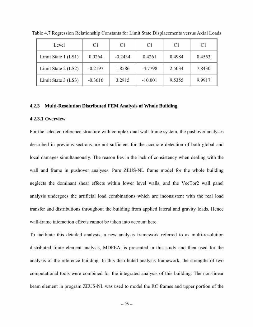
-- 98 --
Table 4.7 Regression Relationship Constants for Limit State Displacements versus Axial Loads
Level C1 C1 C1 C1 C1
Limit State 1 (LS1) 0.0264 -0.2434 0.4261 0.4984 0.4553
Limit State 2 (LS2) -0.2197 1.8586 -4.7798 2.5034 7.8430
Limit State 3 (LS3) -0.3616 3.2815 -10.001 9.5355 9.9917
4.2.3 Multi-Resolution Distributed FEM Analysis of Whole Building
4.2.3.1 Overview
For the selected reference structure with complex dual wall-frame system, the pushover analyses
described in previous sections are not sufficient for the accurate detection of both global and
local damages simultaneously. The reason lies in the lack of consistency when dealing with the
wall and frame in pushover analyses. Pure ZEUS-NL frame model for the whole building
neglects the dominant shear effects within lower level walls, and the VecTor2 wall panel
analysis undergoes the artificial load combinations which are inconsistent with the real load
transfer and distributions throughout the building from applied lateral and gravity loads. Hence
wall-frame interaction effects cannot be taken into account here.
To facilitate this detailed analysis, a new analysis framework referred to as multi-resolution
distributed finite element analysis, MDFEA, is presented in this study and then used for the
analysis of the reference building. In this distributed analysis framework, the strengths of two
computational tools were combined for the integrated analysis of this building. The non-linear
beam element in program ZEUS-NL was used to model the RC frames and upper portion of the
-- 99 --
RC walls while the non-linear continuum analysis program VecTor2 was used to model the lower
portions of the building’s RC shear walls. The combined use of these two different programs was
made possible by the development of a ‘simulation coordinator’ program that can seamlessly
merge multiple computational components into one structural system. The latter coordinator,
UI-SIMCOR developed by Kwon et al. (2005), runs several concurrent components, combining
their action-deformation characteristics on a network.
4.2.3.2 Detailed Algorithm
Different state-of-the-art analysis software packages have unique features that other competing
packages do not have. Similarly, different research laboratories are equipped with unique
experimental facilities that complement each other. The main advantage of multi-platform
simulation is the use of the unique features of analytical tools and/or experimental facilities in an
integrated fashion, an essence of the distributed Network for Earthquake Engineering
Simulations (NEES). The concept of multi-platform simulation is implemented using the
pseudo-dynamic (PSD) simulation approach combined with sub-structuring. In the latter
simulation, a structure is subdivided into several modules that are either physically tested or
computationally simulated. UI-SIMCOR (Kwon et al. (2005)) was developed for this purpose.
The Operator Splitting method in conjunction with the α-modified Newmark scheme (α-OS
method) is implemented as a time-stepping analysis scheme. The main feature of UI-SIMCOR is
that it is capable of coordinating any number of analysis tools. Interfaces are currently exist for
ZEUS-NL, OpenSees (McKenna and Fenves (2001)), FedeasLab (Filippou and Constantinides
(2004)), VecTor2, and ABAQUS (Hibbit et al. (2001). Any number of testing sites, or a mixture
-- 100 --
of analysis tools and testing sites can be incorporated into a pseudo-dynamic multi-platform
simulation. It employs software or hardware supporting NEESgrid Teleoperation Control
Protocol (NTCP; by Pearlman et al. (2004)) as well as TCP-IP connections outside of the NEES
system. It is also capable of using the same analysis platform while modeling different parts of
the system on the same or different processors, thus minimizing computational run time. In this
study, UI-SIMCOR is used to combine VecTor2 and ZEUS-NL to model shear-walls and frame
elements.
In the use of UI-SIMCOR, an entire structure is divided into components, which are represented
by different analysis platforms or experimental models. Mesh refinements and DOF numbering
are conducted within sub-structure components. Global stiffness matrix for effective DOFs at
control points is assembled in UI-SIMCOR with control points in the sub-structure models.
Control points are nodes with lumped masses or at the interface between two structural
components. These control points must be defined first in order to form the global mass and
stiffness matrices necessary in pseudo-dynamic (PSD) algorithm employed in UI-SIMCOR, and
to serve as the common interfaces between sub-structures. Hence one important issue in
sub-structuring of RC high-rise buildings is to model the wall-frame interfaces at control points.
For frame elements and solid continuum elements connected at control points,
degree-of-freedom (DOF) coupling must be considered, such as displacements and load transfer
between [u, v, θ] for 2D beam elements and [u’, v’] for 2D solid continuum elements. The details
for modeling this interface are described in Section 3 of this paper within the description of the
complete modeling of 54-story high-rise building example.
-- 101 --
In sub-structured simulation, the structure should be divided into sub-components satisfying two
basic conditions – displacement compatibility and force equilibrium. The multi-platform
simulation framework utilizes unique structural analysis platforms at the user level, which does
not allow iteration for path-dependent nonlinear inelastic models. Hence, Kwon et al. (2005)
employed a method to avoid iterations. UI-SIMCOR takes advantage of the PSD scheme to
combine various analytical platforms and thereby to avoid global nonlinear iterations. Only time
integration scheme is coded inside UI-SIMCOR main framework. Other structural models reside
within external static analysis modules or experimental facilities if hybrid simulation (combined
analysis and experimentation) is engaged. Currently, the α-modified Newmark scheme (α-OS
method) is implemented as the PSD scheme in UI-SIMCOR. The α-OS method follows the
algorithm presented by Combescure and Pegon (1997).
The architecture of the framework is depicted in Figure 4.6. UI-SIMCOR uses object-oriented
programming for easier maintenance and future expansion. There exist two major classes of
modules:
• MDL_RF (restoring force module) represents structural components, with functionalities of
imposing displacement to the structural components and obtaining restoring forces.
• MDL_AUX (auxiliary module) controls experimental hardware other than actuators, which
is not applicable in this study.
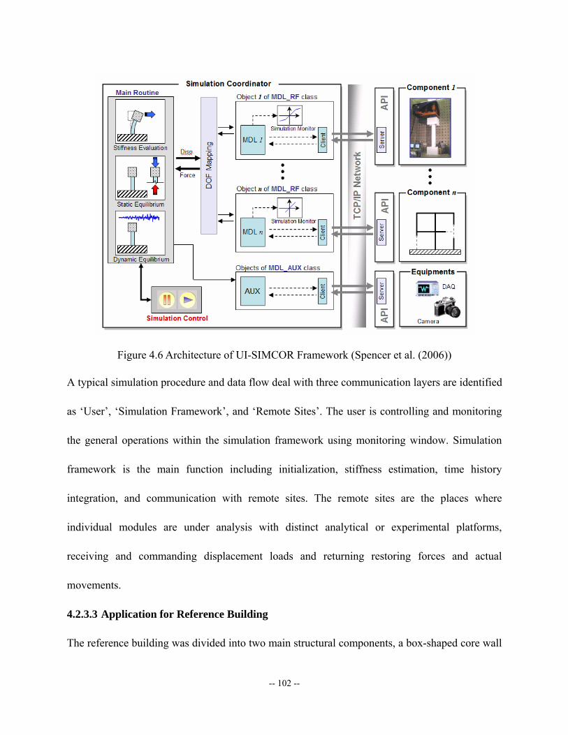
-- 102 --
Figure 4.6 Architecture of UI-SIMCOR Framework (Spencer et al. (2006))
A typical simulation procedure and data flow deal with three communication layers are identified
as ‘User’, ‘Simulation Framework’, and ‘Remote Sites’. The user is controlling and monitoring
the general operations within the simulation framework using monitoring window. Simulation
framework is the main function including initialization, stiffness estimation, time history
integration, and communication with remote sites. The remote sites are the places where
individual modules are under analysis with distinct analytical or experimental platforms,
receiving and commanding displacement loads and returning restoring forces and actual
movements.
4.2.3.3 Application for Reference Building
The reference building was divided into two main structural components, a box-shaped core wall
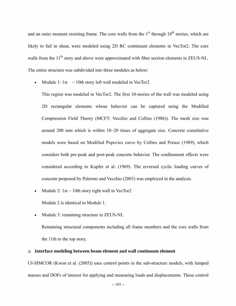
-- 103 --
and an outer moment resisting frame. The core walls from the 1st through 10th stories, which are
likely to fail in shear, were modeled using 2D RC continuum elements in VecTor2. The core
walls from the 11th story and above were approximated with fiber section elements in ZEUS-NL.
The entire structure was subdivided into three modules as below:
• Module 1: 1st ~ 10th story left wall modeled in VecTor2
This region was modeled in VecTor2. The first 10-stories of the wall was modeled using
2D rectangular elements whose behavior can be captured using the Modified
Compression Field Theory (MCFT; Vecchio and Collins (1986)). The mesh size was
around 200 mm which is within 10~20 times of aggregate size. Concrete constitutive
models were based on Modified Popovics curve by Collins and Porasz (1989), which
considers both pre-peak and post-peak concrete behavior. The confinement effects were
considered according to Kupfer et al. (1969). The reversed cyclic loading curves of
concrete proposed by Palermo and Vecchio (2003) was employed in the analysis.
• Module 2: 1st ~ 10th story right wall in VecTor2
Module 2 is identical to Module 1.
• Module 3: remaining structure in ZEUS-NL
Remaining structural components including all frame members and the core walls from
the 11th to the top story.
Interface modeling between beam element and wall continuum element
UI-SIMCOR (Kwon et al. (2005)) uses control points in the sub-structure models, with lumped
masses and DOFs of interest for applying and measuring loads and displacements. These control
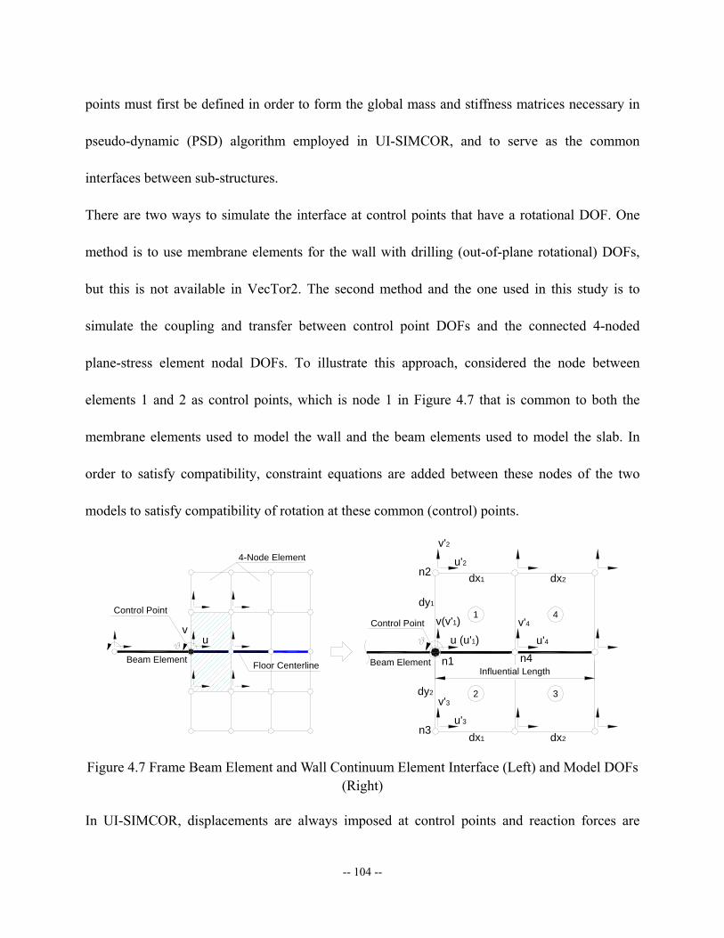
-- 104 --
points must first be defined in order to form the global mass and stiffness matrices necessary in
pseudo-dynamic (PSD) algorithm employed in UI-SIMCOR, and to serve as the common
interfaces between sub-structures.
There are two ways to simulate the interface at control points that have a rotational DOF. One
method is to use membrane elements for the wall with drilling (out-of-plane rotational) DOFs,
but this is not available in VecTor2. The second method and the one used in this study is to
simulate the coupling and transfer between control point DOFs and the connected 4-noded
plane-stress element nodal DOFs. To illustrate this approach, considered the node between
elements 1 and 2 as control points, which is node 1 in Figure 4.7 that is common to both the
membrane elements used to model the wall and the beam elements used to model the slab. In
order to satisfy compatibility, constraint equations are added between these nodes of the two
models to satisfy compatibility of rotation at these common (control) points.
n4
n3
n1
n2
3
4
dx2dx1
Influential Length
dy2
dy1
u'3
v'3
u'4
v'2
u'2
v'4u (u'1)
2
1
Beam Element
Control Point v(v'1)
uv
Floor Centerline
Control Point
4-Node Element
Beam Element
dx1 dx2
Figure 4.7 Frame Beam Element and Wall Continuum Element Interface (Left) and Model DOFs (Right)
In UI-SIMCOR, displacements are always imposed at control points and reaction forces are
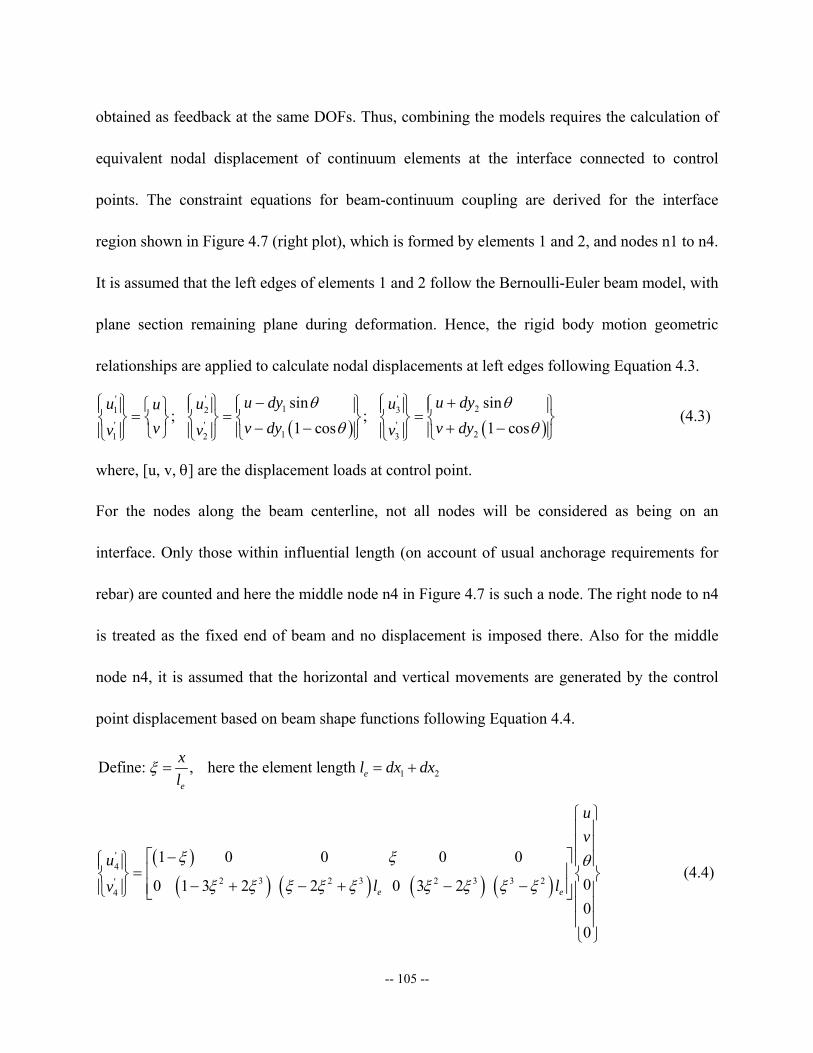
-- 105 --
obtained as feedback at the same DOFs. Thus, combining the models requires the calculation of
equivalent nodal displacement of continuum elements at the interface connected to control
points. The constraint equations for beam-continuum coupling are derived for the interface
region shown in Figure 4.7 (right plot), which is formed by elements 1 and 2, and nodes n1 to n4.
It is assumed that the left edges of elements 1 and 2 follow the Bernoulli-Euler beam model, with
plane section remaining plane during deformation. Hence, the rigid body motion geometric
relationships are applied to calculate nodal displacements at left edges following Equation 4.3.
( ) ( )
'' '1 231 2
' ' '1 21 2 3
sin sin; ;
1 cos 1 cosu dy u dyuu uuv dy v dyvv v v
θ θθ θ
− +⎧ ⎫⎧ ⎫ ⎧ ⎫ ⎧ ⎫ ⎧ ⎫⎧ ⎫⎪ ⎪ ⎪ ⎪ ⎪ ⎪ ⎪ ⎪ ⎪ ⎪= = =⎨ ⎬ ⎨ ⎬ ⎨ ⎬ ⎨ ⎬ ⎨ ⎬ ⎨ ⎬− − + −⎪ ⎪ ⎪ ⎪⎪ ⎪ ⎪ ⎪⎩ ⎭ ⎪ ⎪⎩ ⎭ ⎩ ⎭⎩ ⎭ ⎩ ⎭ ⎩ ⎭ (4.3)
where, [u, v, θ] are the displacement loads at control point.
For the nodes along the beam centerline, not all nodes will be considered as being on an
interface. Only those within influential length (on account of usual anchorage requirements for
rebar) are counted and here the middle node n4 in Figure 4.7 is such a node. The right node to n4
is treated as the fixed end of beam and no displacement is imposed there. Also for the middle
node n4, it is assumed that the horizontal and vertical movements are generated by the control
point displacement based on beam shape functions following Equation 4.4.
1 2Define: , here the element length ee
x l dx dxl
ξ = = +
( )( ) ( ) ( ) ( )
'4
2 3 2 3 2 3 3 2'4
1 0 0 0 0
00 1 3 2 2 0 3 2 00
e e
uv
ul lv
ξ ξ θξ ξ ξ ξ ξ ξ ξ ξ ξ
⎧ ⎫⎪ ⎪⎪ ⎪
−⎡ ⎤⎧ ⎫ ⎪ ⎪⎪ ⎪ ⎢ ⎥=⎨ ⎬ ⎨ ⎬− + − + − −⎢ ⎥⎪ ⎪ ⎪ ⎪⎩ ⎭ ⎣ ⎦
⎪ ⎪⎪ ⎪⎩ ⎭
(4.4)
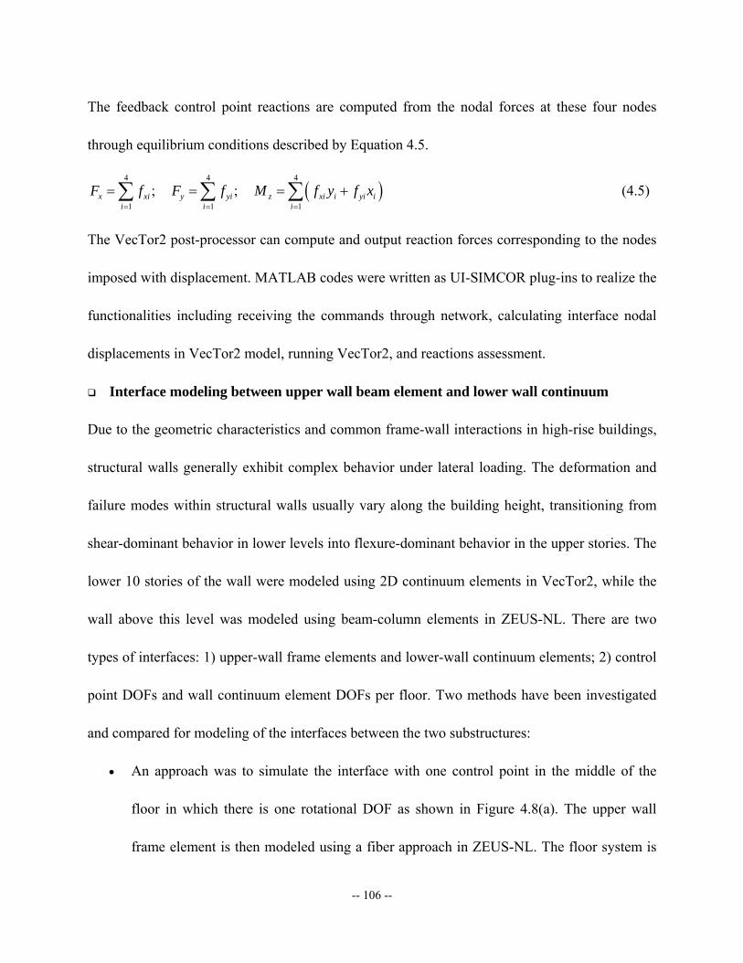
-- 106 --
The feedback control point reactions are computed from the nodal forces at these four nodes
through equilibrium conditions described by Equation 4.5.
( )4 4 4
1 1 1
; ; x xi y yi z xi i yi ii i i
F f F f M f y f x= = =
= = = +∑ ∑ ∑ (4.5)
The VecTor2 post-processor can compute and output reaction forces corresponding to the nodes
imposed with displacement. MATLAB codes were written as UI-SIMCOR plug-ins to realize the
functionalities including receiving the commands through network, calculating interface nodal
displacements in VecTor2 model, running VecTor2, and reactions assessment.
Interface modeling between upper wall beam element and lower wall continuum
Due to the geometric characteristics and common frame-wall interactions in high-rise buildings,
structural walls generally exhibit complex behavior under lateral loading. The deformation and
failure modes within structural walls usually vary along the building height, transitioning from
shear-dominant behavior in lower levels into flexure-dominant behavior in the upper stories. The
lower 10 stories of the wall were modeled using 2D continuum elements in VecTor2, while the
wall above this level was modeled using beam-column elements in ZEUS-NL. There are two
types of interfaces: 1) upper-wall frame elements and lower-wall continuum elements; 2) control
point DOFs and wall continuum element DOFs per floor. Two methods have been investigated
and compared for modeling of the interfaces between the two substructures:
• An approach was to simulate the interface with one control point in the middle of the
floor in which there is one rotational DOF as shown in Figure 4.8(a). The upper wall
frame element is then modeled using a fiber approach in ZEUS-NL. The floor system is
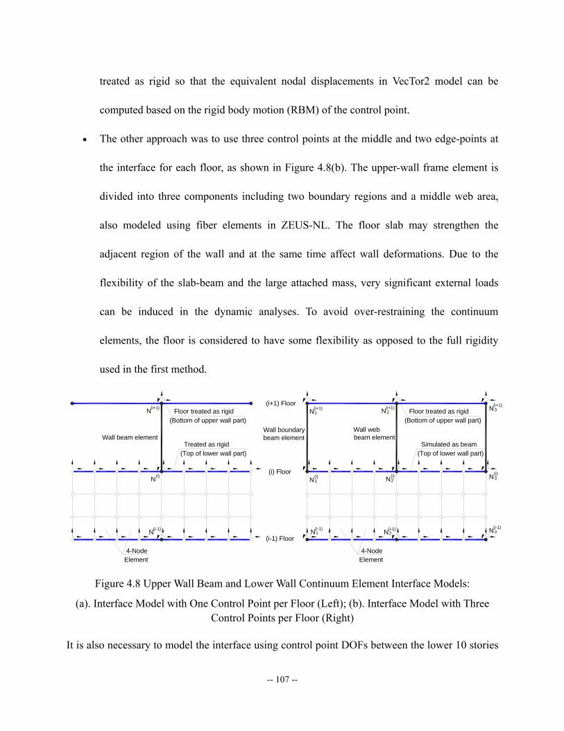
-- 107 --
treated as rigid so that the equivalent nodal displacements in VecTor2 model can be
computed based on the rigid body motion (RBM) of the control point.
• The other approach was to use three control points at the middle and two edge-points at
the interface for each floor, as shown in Figure 4.8(b). The upper-wall frame element is
divided into three components including two boundary regions and a middle web area,
also modeled using fiber elements in ZEUS-NL. The floor slab may strengthen the
adjacent region of the wall and at the same time affect wall deformations. Due to the
flexibility of the slab-beam and the large attached mass, very significant external loads
can be induced in the dynamic analyses. To avoid over-restraining the continuum
elements, the floor is considered to have some flexibility as opposed to the full rigidity
used in the first method.
Floor treated as rigid(Bottom of upper wall part)
4-Node
N(i+1)
(Top of lower wall part)Treated as rigid
Wall beam element
(i-1)N3(i-1)N21N(i-1)
(i)N3(i)N21N(i)
(i-1) Floor
Floor treated as rigid(Bottom of upper wall part)
(i) Floor
(i+1) Floor(i+1)N1 2N(i+1) 3N(i+1)
(Top of lower wall part)Simulated as beam
Wall boundarybeam element beam element
Wall web
4-NodeElementElement
(i-1)N
(i)N
Figure 4.8 Upper Wall Beam and Lower Wall Continuum Element Interface Models:
(a). Interface Model with One Control Point per Floor (Left); (b). Interface Model with Three Control Points per Floor (Right)
It is also necessary to model the interface using control point DOFs between the lower 10 stories

-- 108 --
of the wall that were modeled using continuum elements in VecTor2 and the upper stories that
were modeled by beam-column elements in ZEUS-NL. This interface is described in Figure 4.9.
As with the previous discussed interface, it is necessary to select a pattern of displacements of
the interface nodes along the interface, in this case floor centerline, in the VecTor2 model. Once
again, the two previously described methods are considered.
Bxj
v'ju'j 2
(i) Floor(i)N1 2N (i) 3N (i)
v2(i)
(i)2u
(i)(i)1 u1
(i) (i)1v (i)
3 u3(i)
(i)3v
Cubic shape function
(i) Floor(i)N
Slab beam treated as rigid
(i)2v
u2(i)(i)
2v'j
u'j
xj
B
Figure 4.9 Wall Interface Interpolation Approaches and DOFs
(a). One-control-point Approach (Upper). (b). Three-control-point Approach (Lower)
• One-control-point approach
In this approach, the rigid body motion assumption is made for the floor slab system as shown in
Figure 4.9(a). The rotational DOF at this control point will generate a linear variation in vertical
displacements at all nodes along the ith floor. The constraint equations for both upper wall to
lower wall and inter-storey lower wall interfaces are derived using Equation 4.6. The control
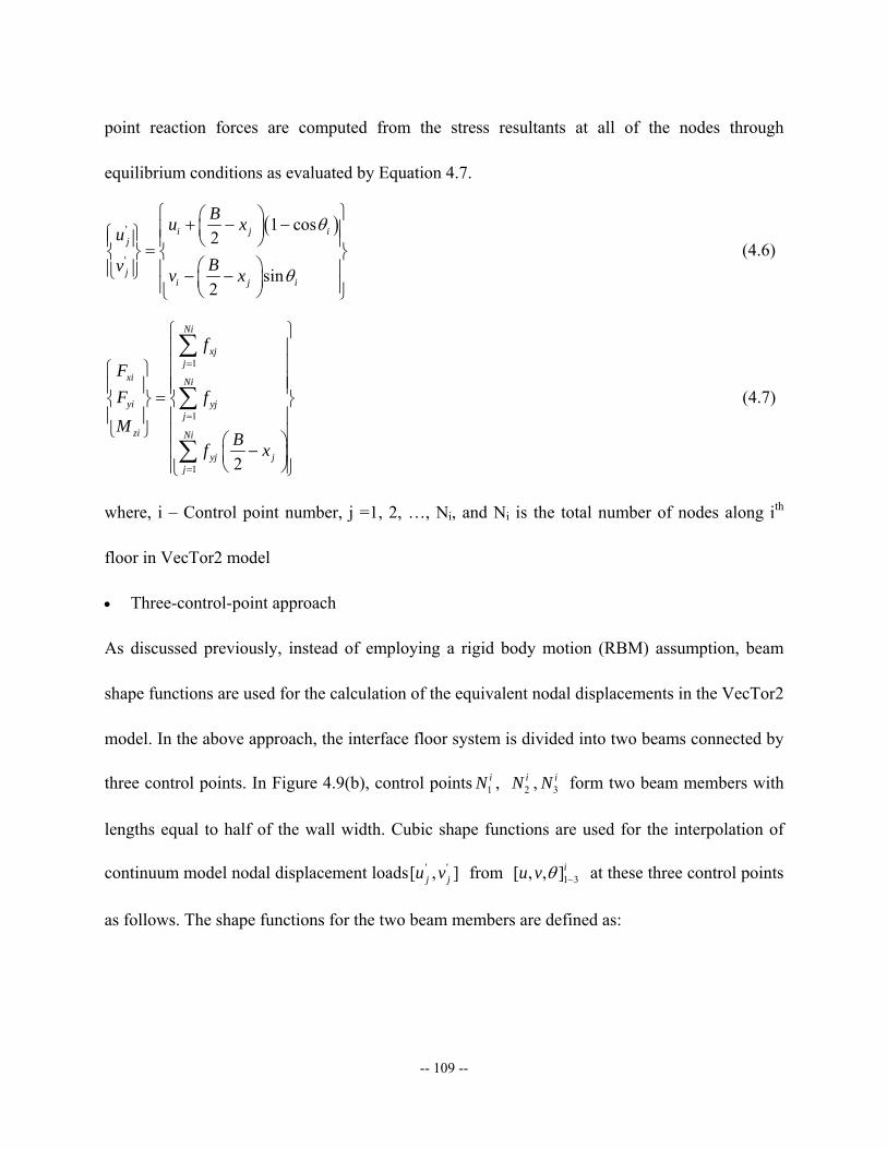
-- 109 --
point reaction forces are computed from the stress resultants at all of the nodes through
equilibrium conditions as evaluated by Equation 4.7.
( )'
'
1 cos2
sin2
i j ij
ji j i
Bu xu
Bv v x
θ
θ
⎧ ⎫⎛ ⎞+ − −⎜ ⎟⎪ ⎪⎧ ⎫⎪ ⎪ ⎪ ⎝ ⎠ ⎪=⎨ ⎬ ⎨ ⎬⎛ ⎞⎪ ⎪ ⎪ ⎪⎩ ⎭ − −⎜ ⎟⎪ ⎪⎝ ⎠⎩ ⎭
(4.6)
1
1
1 2
Ni
xjj
xi Ni
yi yjj
zi Ni
yj jj
fFF f
MBf x
=
=
=
⎧ ⎫⎪ ⎪⎪ ⎪⎧ ⎫⎪ ⎪⎪ ⎪ ⎪ ⎪=⎨ ⎬ ⎨ ⎬
⎪ ⎪ ⎪ ⎪⎩ ⎭ ⎪ ⎪⎛ ⎞⎪ − ⎪⎜ ⎟
⎝ ⎠⎪ ⎪⎩ ⎭
∑
∑
∑
(4.7)
where, i – Control point number, j =1, 2, …, Ni, and Ni is the total number of nodes along ith
floor in VecTor2 model
• Three-control-point approach
As discussed previously, instead of employing a rigid body motion (RBM) assumption, beam
shape functions are used for the calculation of the equivalent nodal displacements in the VecTor2
model. In the above approach, the interface floor system is divided into two beams connected by
three control points. In Figure 4.9(b), control points 1iN , 2
iN , 3iN form two beam members with
lengths equal to half of the wall width. Cubic shape functions are used for the interpolation of
continuum model nodal displacement loads ' '[ , ]j ju v from 1~3[ , , ]iu v θ at these three control points
as follows. The shape functions for the two beam members are defined as:
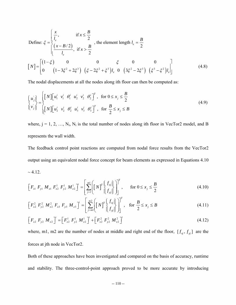
-- 110 --
( )
, if 2
Define: , the element length / 2 2
, if 2
ee
e
x Bxl Blx B Bx
l
ξ
⎧ ≤⎪⎪= =⎨ −⎪ >⎪⎩
[ ]( )
( ) ( ) ( ) ( )2 3 2 3 2 3 3 2
1 0 0 0 0
0 1 3 2 2 0 3 2 e e
Nl l
ξ ξ
ξ ξ ξ ξ ξ ξ ξ ξ ξ
−⎡ ⎤⎢ ⎥=
− + − + − −⎢ ⎥⎣ ⎦ (4.8)
The nodal displacements at all the nodes along ith floor can then be computed as:
[ ]
[ ]
' 1 1 1 2 2 2
'
2 2 2 3 3 3
, for 02
, for 2
Ti i i i i ij
j
Ti i i i i ijj
BN u v u v xu
Bv N u v u v x B
θ θ
θ θ
⎧ ⎡ ⎤ ≤ ≤⎧ ⎫ ⎣ ⎦⎪⎪ ⎪ ⎪=⎨ ⎬ ⎨⎪ ⎪ ⎪⎩ ⎭ ⎡ ⎤ ≤ ≤⎣ ⎦⎪⎩
(4.9)
where, j = 1, 2, …, Ni, Ni is the total number of nodes along ith floor in VecTor2 model, and B
represents the wall width.
The feedback control point reactions are computed from nodal force results from the VecTor2
output using an equivalent nodal force concept for beam elements as expressed in Equations 4.10
~ 4.12.
[ ]1
1 1 11 1 1 2 2 2
1 , for 0
2
Tmi xjT
x y z x y z jj yj
f BF F M F F M N xf=
⎡ ⎤⎛ ⎞⎧ ⎫⎪ ⎪⎡ ⎤ ⎢ ⎥= ≤ ≤⎜ ⎟⎨ ⎬⎣ ⎦ ⎜ ⎟⎢ ⎥⎪ ⎪⎩ ⎭⎝ ⎠⎣ ⎦∑ (4.10)
[ ]2
2 2 22 2 2 3 3 3
1 , for
2
Tmi xjT
x y z x y z jj m yj
f BF F M F F M N x Bf=
⎡ ⎤⎛ ⎞⎧ ⎫⎪ ⎪⎡ ⎤ ⎢ ⎥= ≤ ≤⎜ ⎟⎨ ⎬⎣ ⎦ ⎜ ⎟⎢ ⎥⎪ ⎪⎩ ⎭⎝ ⎠⎣ ⎦∑ (4.11)
1 1 1 2 2 22 2 2 2 2 2 2 2 2
i ii
x y z x y z x y zF F M F F M F F M⎡ ⎤ ⎡ ⎤⎡ ⎤ = +⎣ ⎦ ⎣ ⎦ ⎣ ⎦ (4.12)
where, m1, m2 are the number of nodes at middle and right end of the floor, [ , ]xj yjf f are the
forces at jth node in VecTor2.
Both of these approaches have been investigated and compared on the basis of accuracy, runtime
and stability. The three-control-point approach proved to be more accurate by introducing
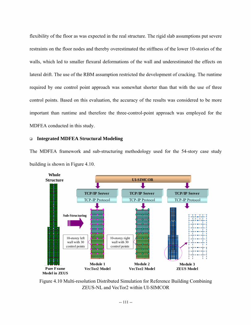
-- 111 --
flexibility of the floor as was expected in the real structure. The rigid slab assumptions put severe
restraints on the floor nodes and thereby overestimated the stiffness of the lower 10-stories of the
walls, which led to smaller flexural deformations of the wall and underestimated the effects on
lateral drift. The use of the RBM assumption restricted the development of cracking. The runtime
required by one control point approach was somewhat shorter than that with the use of three
control points. Based on this evaluation, the accuracy of the results was considered to be more
important than runtime and therefore the three-control-point approach was employed for the
MDFEA conducted in this study.
Integrated MDFEA Structural Modeling
The MDFEA framework and sub-structuring methodology used for the 54-story case study
building is shown in Figure 4.10.
UI-SIMCOR
TCP-IP Protocol
TCP/IP Server
TCP-IP Protocol
TCP/IP Server
Whole Structure
Module 1 VecTor2 Model
10-storey left wall with 30
control points
Module 3 ZEUS Model
TCP-IP Protocol
TCP/IP Server
Module 2 VecTor2 Model
10-storey right wall with 30
control points
Pure Frame Model in ZEUS
Sub-Structuring
Figure 4.10 Multi-resolution Distributed Simulation for Reference Building Combining ZEUS-NL and VecTor2 within UI-SIMCOR
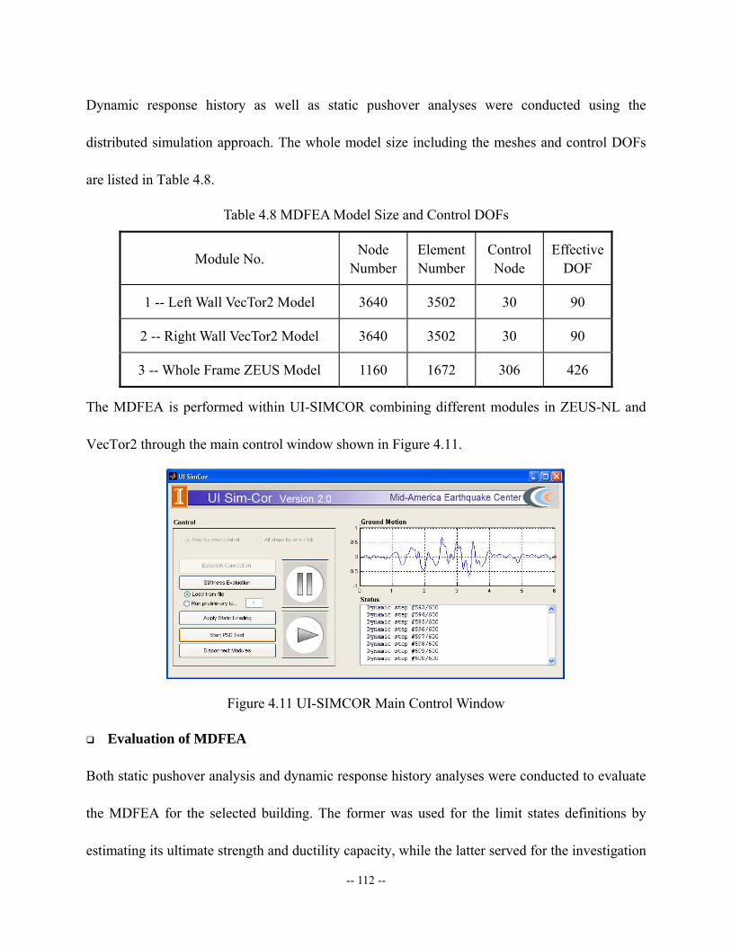
-- 112 --
Dynamic response history as well as static pushover analyses were conducted using the
distributed simulation approach. The whole model size including the meshes and control DOFs
are listed in Table 4.8.
Table 4.8 MDFEA Model Size and Control DOFs
Module No. Node Number
Element Number
Control Node
Effective DOF
1 -- Left Wall VecTor2 Model 3640 3502 30 90
2 -- Right Wall VecTor2 Model 3640 3502 30 90
3 -- Whole Frame ZEUS Model 1160 1672 306 426
The MDFEA is performed within UI-SIMCOR combining different modules in ZEUS-NL and
VecTor2 through the main control window shown in Figure 4.11.
Figure 4.11 UI-SIMCOR Main Control Window
Evaluation of MDFEA
Both static pushover analysis and dynamic response history analyses were conducted to evaluate
the MDFEA for the selected building. The former was used for the limit states definitions by
estimating its ultimate strength and ductility capacity, while the latter served for the investigation

-- 113 --
of real building behavior under selected representative ground motion records.
• Static pushover analysis
In UI-SIMCOR, gravity loads were applied to the building prior to conducting this static
pushover analysis, as shown in Figure 4.12. Static Loading History
0
0.2
0.4
0.6
0.8
1
1.2
0 10 20 30 40 50 60 70 80 90 100 110 120 130
Load Steps
Load
Fac
tor
Gravity LoadingPush-over Loading
Figure 4.12 Static Loading Histories in MDFEA
Two analyses were conducted in the study, one using the MDFEA framework and the other in
which the structure was entirely modeled as a frame using ZEUS-NL. A comparison of the
results from these analyses is presented in Figure 4.13.
These comparisons illustrate that the lateral drift in the lower part of the wall has more flexibility
and ductility in MDFEA than in the ZEUS-NL analysis. This is mainly due to the much larger
shear deformation contributions that were captured in the continuum model of the MDFEA. At
higher load levels, the ZEUS-NL model exhibits lower stiffness and ultimately less strength than
the MDFEA model. This is mainly because the plane section assumption in the fiber approach
leads to concrete crushing at the base of the wall before the concrete compressive capacity is
reached in accordance to the continuum model.
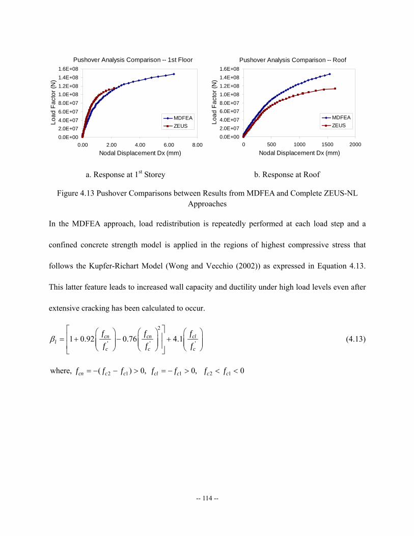
-- 114 --
Pushover Analysis Comparison -- 1st Floor
0.0E+002.0E+074.0E+076.0E+078.0E+071.0E+081.2E+081.4E+081.6E+08
0.00 2.00 4.00 6.00 8.00Nodal Displacement Dx (mm)
Load
Fac
tor (
N)
MDFEAZEUS
Pushover Analysis Comparison -- Roof
0.0E+002.0E+074.0E+076.0E+078.0E+071.0E+081.2E+081.4E+081.6E+08
0 500 1000 1500 2000
Nodal Displacement Dx (mm)
Load
Fac
tor (
N)
MDFEAZEUS
a. Response at 1st Storey b. Response at Roof
Figure 4.13 Pushover Comparisons between Results from MDFEA and Complete ZEUS-NL Approaches
In the MDFEA approach, load redistribution is repeatedly performed at each load step and a
confined concrete strength model is applied in the regions of highest compressive stress that
follows the Kupfer-Richart Model (Wong and Vecchio (2002)) as expressed in Equation 4.13.
This latter feature leads to increased wall capacity and ductility under high load levels even after
extensive cracking has been calculated to occur.
2
' ' '1 0.92 0.76 4.1cn cn cll
c c c
f f ff f f
β⎡ ⎤⎛ ⎞ ⎛ ⎞ ⎛ ⎞⎢ ⎥= + − +⎜ ⎟ ⎜ ⎟ ⎜ ⎟⎜ ⎟ ⎜ ⎟ ⎜ ⎟⎢ ⎥⎝ ⎠ ⎝ ⎠ ⎝ ⎠⎣ ⎦
(4.13)
2 1 1 2 1where, ( ) 0, 0, 0cn c c cl c c cf f f f f f f= − − > = − > < <
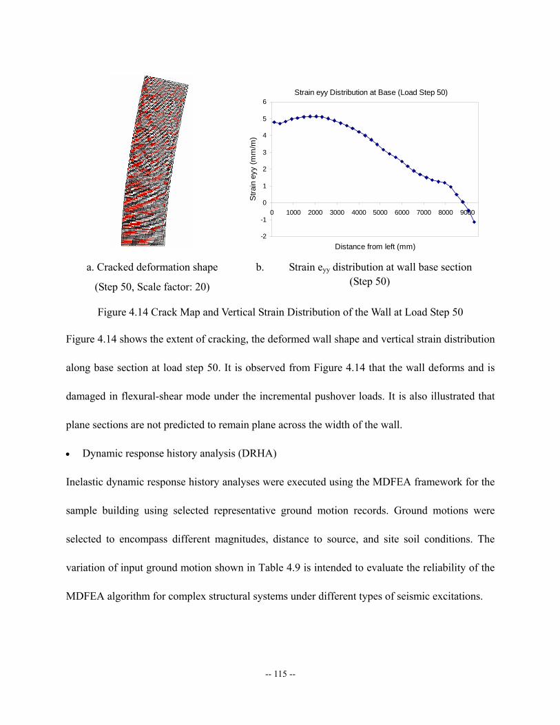
-- 115 --
Strain eyy Distribution at Base (Load Step 50)
-2
-1
0
1
2
3
4
5
6
0 1000 2000 3000 4000 5000 6000 7000 8000 9000
Distance from left (mm)S
train
eyy
(mm
/m)
a. Cracked deformation shape
(Step 50, Scale factor: 20)
b. Strain eyy distribution at wall base section (Step 50)
Figure 4.14 Crack Map and Vertical Strain Distribution of the Wall at Load Step 50
Figure 4.14 shows the extent of cracking, the deformed wall shape and vertical strain distribution
along base section at load step 50. It is observed from Figure 4.14 that the wall deforms and is
damaged in flexural-shear mode under the incremental pushover loads. It is also illustrated that
plane sections are not predicted to remain plane across the width of the wall.
• Dynamic response history analysis (DRHA)
Inelastic dynamic response history analyses were executed using the MDFEA framework for the
sample building using selected representative ground motion records. Ground motions were
selected to encompass different magnitudes, distance to source, and site soil conditions. The
variation of input ground motion shown in Table 4.9 is intended to evaluate the reliability of the
MDFEA algorithm for complex structural systems under different types of seismic excitations.
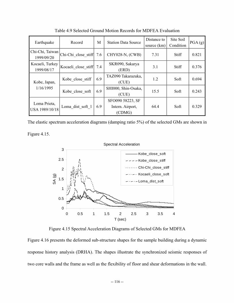
-- 116 --
Table 4.9 Selected Ground Motion Records for MDFEA Evaluation
Earthquake Record M Station Data Source Distance to source (km)
Site Soil Condition
PGA (g)
Chi-Chi, Taiwan 1999/09/20
Chi-Chi_close_stiff 7.6 CHY028-N, (CWB) 7.31 Stiff 0.821
Kocaeli, Turkey 1999/08/17
Kocaeli_close_stiff 7.4 SKR090, Sakarya
(ERD) 3.1 Stiff 0.376
Kobe_close_stiff 6.9 TAZ090 Takarazuka,
(CUE) 1.2 Soft 0.694
Kobe, Japan, 1/16/1995
Kobe_close_soft 6.9 SHI000, Shin-Osaka,
(CUE) 15.5 Soft 0.243
Loma Prieta, USA 1989/10/18
Loma_dist_soft_1 6.9 SFO090 58223, SF
Intern. Airport, (CDMG)
64.4 Soft 0.329
The elastic spectrum acceleration diagrams (damping ratio 5%) of the selected GMs are shown in
Figure 4.15.
Spectral Acceleration
0
0.5
1
1.5
2
2.5
3
0 0.5 1 1.5 2 2.5 3 3.5 4T (sec)
SA
(g)
Kobe_close_soft
Kobe_close_stiff
Chi-Chi_close_stiff
Kocaeli_close_soft
Loma_dist_soft
Figure 4.15 Spectral Acceleration Diagrams of Selected GMs for MDFEA
Figure 4.16 presents the deformed sub-structure shapes for the sample building during a dynamic
response history analysis (DRHA). The shapes illustrate the synchronized seismic responses of
two core walls and the frame as well as the flexibility of floor and shear deformations in the wall.
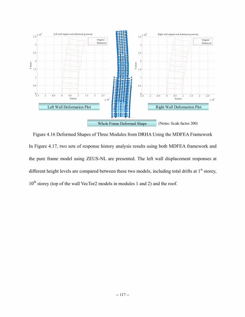
-- 117 --
-1.5 -1 -0.5 0 0.5 1 1.5 2 2.5
x 104
0
0.5
1
1.5
2
2.5
3
3.5x 10
4
X (mm)
Y (m
m)
Left wall original and deformed geometry
OriginalDeformed
-1.5 -1 -0.5 0 0.5 1 1.5 2 2.5
x 104
0
0.5
1
1.5
2
2.5
3
3.5x 10
4
X (mm)
Y (m
m)
Right wall original and deformed geometry
OriginalDeformed
Left Wall Deformation Plot Right Wall Deformation Plot
(Notes: Scale factor 200)Whole Frame Deformed Shape
Figure 4.16 Deformed Shapes of Three Modules from DRHA Using the MDFEA Framework
In Figure 4.17, two sets of response history analysis results using both MDFEA framework and
the pure frame model using ZEUS-NL are presented. The left wall displacement responses at
different height levels are compared between these two models, including total drifts at 1st storey,
10th storey (top of the wall VecTor2 models in modules 1 and 2) and the roof.

-- 118 --
Displacement History -- 1st Floor (Left wall)
-2-1.5
-1-0.5
00.5
11.5
2
0 1 2 3 4 5 6
Time (sec)
Dx
(mm
)
ZEUSMDFEA
Displacement History -- 1st Floor (Left wall)
-2-1.5
-1-0.5
00.5
11.5
2
0 1 2 3 4 5 6 7 8 9 10
Time (sec)
Dx
(mm
)
ZEUSMDFEA
Displacement History -- 10th Floor (Left wall)
-80-60-40-20
020406080
0 1 2 3 4 5 6
Time (sec)
Dx
(mm
)
ZEUSMDFEA
Displacement History -- 10th Floor (Left wall)
-80-60-40-20
020406080
0 1 2 3 4 5 6 7 8 9 10
Time (sec)
Dx
(mm
)
ZEUSMDFEA
Displacement History -- Roof (Left wall)
-600
-400
-200
0
200
400
600
0 1 2 3 4 5 6
Time (sec)
Dx
(mm
)
ZEUSMDFEA
Displacement History -- Roof (Left wall)
-600
-400
-200
0
200
400
600
0 1 2 3 4 5 6 7 8 9 10
Time (sec)
Dx
(mm
)
ZEUSMDFEA
a. Seismic responses imposed with GM record Kobe_close_stiff
b. Seismic responses imposed with GM record Kobe_close_soft
Figure 4.17 Sample Displacement Histories and Comparisons between MDFEA and ZEUS-NL Approaches
The results presented in Figure 13 illustrate that the drift computed from MDFEA at the lower
levels is much larger than that from ZEUS-NL pure frame model, while the roof drifts from the
two models are relatively close.
The comparisons presented above illustrate that pure-frame analyses neglect important and
critical features of the response of the 54-story high-rise building. The MDFEA procedure can
account for response limit states including shear-flexure-axial interaction and can serve as the
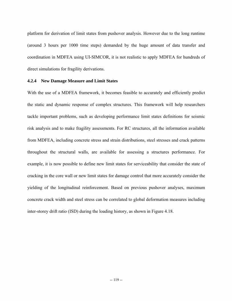
-- 119 --
platform for derivation of limit states from pushover analysis. However due to the long runtime
(around 3 hours per 1000 time steps) demanded by the huge amount of data transfer and
coordination in MDFEA using UI-SIMCOR, it is not realistic to apply MDFEA for hundreds of
direct simulations for fragility derivations.
4.2.4 New Damage Measure and Limit States
With the use of a MDFEA framework, it becomes feasible to accurately and efficiently predict
the static and dynamic response of complex structures. This framework will help researchers
tackle important problems, such as developing performance limit states definitions for seismic
risk analysis and to make fragility assessments. For RC structures, all the information available
from MDFEA, including concrete stress and strain distributions, steel stresses and crack patterns
throughout the structural walls, are available for assessing a structures performance. For
example, it is now possible to define new limit states for serviceability that consider the state of
cracking in the core wall or new limit states for damage control that more accurately consider the
yielding of the longitudinal reinforcement. Based on previous pushover analyses, maximum
concrete crack width and steel stress can be correlated to global deformation measures including
inter-storey drift ratio (ISD) during the loading history, as shown in Figure 4.18.
-- 120 --
Maximum Crack Width vs. Maximum ISD
0
1
2
3
4
5
6
7
8
0 0.1 0.2 0.3 0.4 0.5 0.6 0.7 0.8 0.9 1
Maximum ISD (%)
Max
imum
Wcr
(mm
)First crack
>0.2mm point
Maximum Steel Stress vs. Maximum ISD
050
100150200250300350400450500
0 0.1 0.2 0.3 0.4 0.5 0.6 0.7 0.8 0.9 1
Maximum ISD (%)
Max
imum
Ss
(Mpa
)
First steel yielding point
a. Limit State 1 – Serviceability by Considerable Cracking (Wcr > 0.2mm)
b. Limit State 2 – Damage Control by Wall Rebar Yielding (fy >= 460 MPa)
Figure 4.18 Quantitative Definitions for Limit States 1 and 2 Using MDFEA Results
For high-rise buildings, it is insufficient to use traditional definitions of ISD for damage measure
of the structural performances. The reason is due to the nature of two major sources contributing
to the ISD: (1) lateral translations by shear and flexural deformation; and (2) translations from
rigid body motion (RBM) due to lower storey rotation. The first one relates structural
deformations to member stress and strain resultants, while the latter one does not contribute to
structural demand. Figure 4.19 presents the relationship between the right wall shear and
inter-storey drift, pure translation component, lower storey rotation, and the ratio of the rotation
effect to overall drift. As shown, the total inter-storey drift at level 10 increases to 33 mm while
that at the 1st level is only 3.3 mm. The ratio of ISD by lower storey rotation to total ISD rises up
from 0.0 at the 1st storey, to 0.68 at the 2nd storey, to 0.97 at the 10th storey. The drift from pure
translations at 10th storey is only about 1.5 mm. This illustrates that for high-rise buildings the
traditional measure of total ISD cannot be directly related to structural performance.

-- 121 --
0 5 10 15 20 25 30 350
0.5
1
1.5
2
2.5
3
3.5x 10⁴
Inter-storey Drift (mm)
Wal
l She
ar (k
N)
Vwall vs. ISD
0 5 10 15 20 25 30 350
0.5
1
1.5
2
2.5
3
3.5x 10⁴
Inter-storey Drift (mm)
Wal
l She
ar (k
N)
Vwall vs. ISD by lower storey rotation
0 0.5 1 1.5 2 2.5 3 3.50
0.5
1
1.5
2
2.5
3
3.5x 10⁴
Inter-storey Drift (mm)
Wal
l She
ar (k
N)
Vwall vs. ISD by pure translation
0 0.2 0.4 0.6 0.8 10
0.5
1
1.5
2
2.5
3
3.5x 10⁴
Ratio of Rotation effect to total drift
Wal
l She
ar (k
N)
Vwall vs. Rotation effect
Wall2 in Storey 1Wall2 in Storey 2Wall2 in Storey 4Wall2 in Storey 6Wall2 in Storey 8Wall2 in Storey 10
Wall2 in Storey 1Wall2 in Storey 2Wall2 in Storey 4Wall2 in Storey 8Wall2 in Storey 10
Wall2 in Storey 1Wall2 in Storey 2Wall2 in Storey 4Wall2 in Storey 6Wall2 in Storey 8Wall2 in Storey 10
Wall2 in Storey 1Wall2 in Storey 2Wall2 in Storey 4Wall2 in Storey 6Wall2 in Storey 8Wall2 in Storey 10
Figure 4.19 Wall Shear versus Inter-storey Drift (ISD) and Drift Components Evaluation
In this study a new measure called inter-storey pure translation ratio (ISPT) is proposed by
removing the RBM due to lower storey rotation. ISPT is computed from post-processed member
(mainly wall) deformation data as shown in Figure 4.20 and Equation 4.14.
[ ]11 1 1 1
1
( sin )1 (1 cos ) ( sin ) tan sincos
i ii i i i
i
dx HISPT dy H dx H
Hθ
θ θ θ θθ
⎡ ⎤−= + − − − −⎢ ⎥
⎣ ⎦ (4.14)
dyi
dxi
θ1
θ1
θ2
dui
i
i+1
Hi
Figure 4.20 Inter-storey Member Deformation Geometry
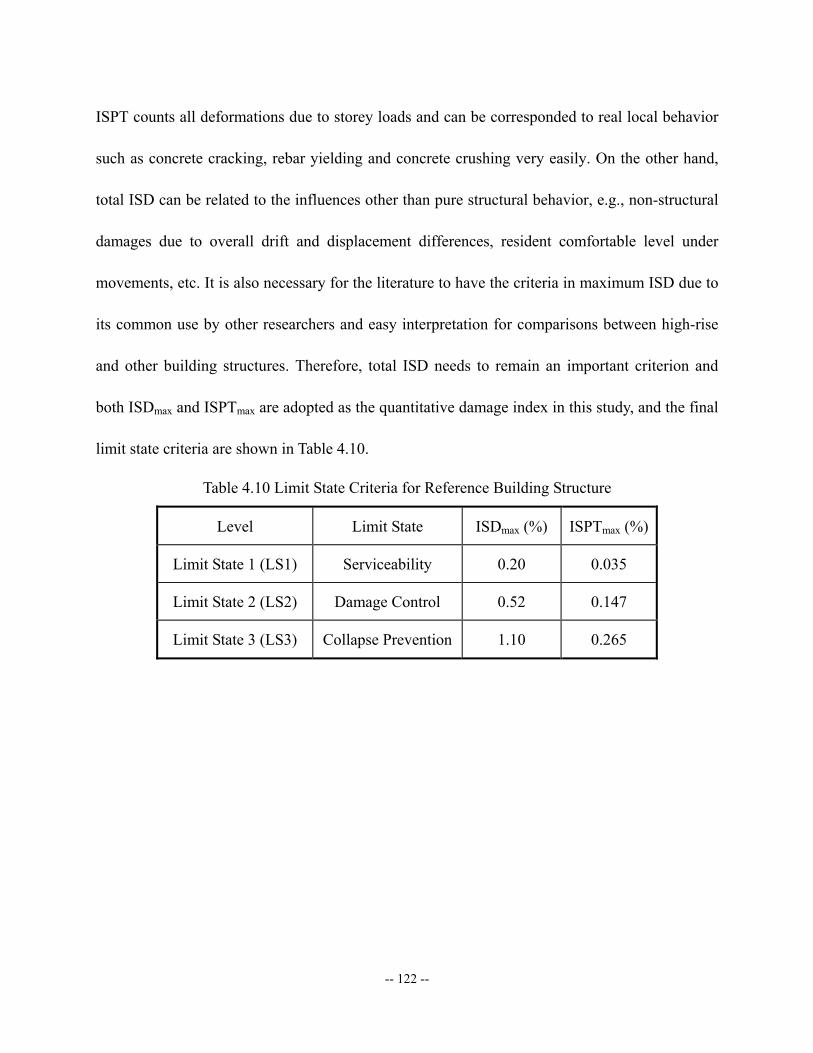
-- 122 --
ISPT counts all deformations due to storey loads and can be corresponded to real local behavior
such as concrete cracking, rebar yielding and concrete crushing very easily. On the other hand,
total ISD can be related to the influences other than pure structural behavior, e.g., non-structural
damages due to overall drift and displacement differences, resident comfortable level under
movements, etc. It is also necessary for the literature to have the criteria in maximum ISD due to
its common use by other researchers and easy interpretation for comparisons between high-rise
and other building structures. Therefore, total ISD needs to remain an important criterion and
both ISDmax and ISPTmax are adopted as the quantitative damage index in this study, and the final
limit state criteria are shown in Table 4.10.
Table 4.10 Limit State Criteria for Reference Building Structure
Level Limit State ISDmax (%) ISPTmax (%)
Limit State 1 (LS1) Serviceability 0.20 0.035
Limit State 2 (LS2) Damage Control 0.52 0.147
Limit State 3 (LS3) Collapse Prevention 1.10 0.265
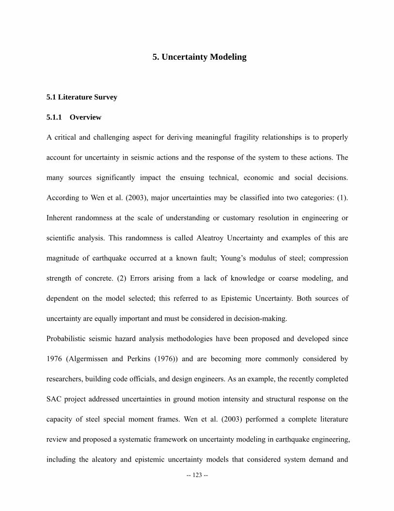
-- 123 --
5. Uncertainty Modeling
5.1 Literature Survey
5.1.1 Overview
A critical and challenging aspect for deriving meaningful fragility relationships is to properly
account for uncertainty in seismic actions and the response of the system to these actions. The
many sources significantly impact the ensuing technical, economic and social decisions.
According to Wen et al. (2003), major uncertainties may be classified into two categories: (1).
Inherent randomness at the scale of understanding or customary resolution in engineering or
scientific analysis. This randomness is called Aleatroy Uncertainty and examples of this are
magnitude of earthquake occurred at a known fault; Young’s modulus of steel; compression
strength of concrete. (2) Errors arising from a lack of knowledge or coarse modeling, and
dependent on the model selected; this referred to as Epistemic Uncertainty. Both sources of
uncertainty are equally important and must be considered in decision-making.
Probabilistic seismic hazard analysis methodologies have been proposed and developed since
1976 (Algermissen and Perkins (1976)) and are becoming more commonly considered by
researchers, building code officials, and design engineers. As an example, the recently completed
SAC project addressed uncertainties in ground motion intensity and structural response on the
capacity of steel special moment frames. Wen et al. (2003) performed a complete literature
review and proposed a systematic framework on uncertainty modeling in earthquake engineering,
including the aleatory and epistemic uncertainty models that considered system demand and
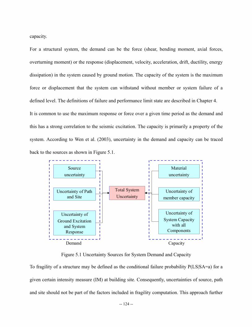
-- 124 --
capacity.
For a structural system, the demand can be the force (shear, bending moment, axial forces,
overturning moment) or the response (displacement, velocity, acceleration, drift, ductility, energy
dissipation) in the system caused by ground motion. The capacity of the system is the maximum
force or displacement that the system can withstand without member or system failure of a
defined level. The definitions of failure and performance limit state are described in Chapter 4.
It is common to use the maximum response or force over a given time period as the demand and
this has a strong correlation to the seismic excitation. The capacity is primarily a property of the
system. According to Wen et al. (2003), uncertainty in the demand and capacity can be traced
back to the sources as shown in Figure 5.1.
Total SystemUncertainty
Material uncertainty
Uncertainty of member capacity
Uncertainty of System Capacity
with all Components
Source uncertainty
Uncertainty of Path and Site
Uncertainty ofGround Excitation
and System Response
Demand Capacity
Figure 5.1 Uncertainty Sources for System Demand and Capacity
To fragility of a structure may be defined as the conditional failure probability P(LS|SA=a) for a
given certain intensity measure (IM) at building site. Consequently, uncertainties of source, path
and site should not be part of the factors included in fragility computation. This approach further
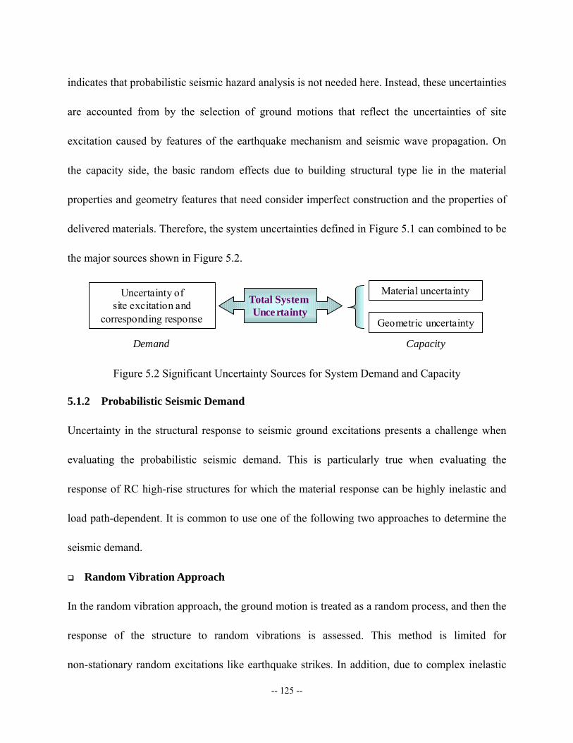
-- 125 --
indicates that probabilistic seismic hazard analysis is not needed here. Instead, these uncertainties
are accounted from by the selection of ground motions that reflect the uncertainties of site
excitation caused by features of the earthquake mechanism and seismic wave propagation. On
the capacity side, the basic random effects due to building structural type lie in the material
properties and geometry features that need consider imperfect construction and the properties of
delivered materials. Therefore, the system uncertainties defined in Figure 5.1 can combined to be
the major sources shown in Figure 5.2.
Total System Uncertainty
Uncertainty of site excitation and
corresponding response
Material uncertainty
Geometric uncertainty
Demand Capacity
Figure 5.2 Significant Uncertainty Sources for System Demand and Capacity
5.1.2 Probabilistic Seismic Demand
Uncertainty in the structural response to seismic ground excitations presents a challenge when
evaluating the probabilistic seismic demand. This is particularly true when evaluating the
response of RC high-rise structures for which the material response can be highly inelastic and
load path-dependent. It is common to use one of the following two approaches to determine the
seismic demand.
Random Vibration Approach
In the random vibration approach, the ground motion is treated as a random process, and then the
response of the structure to random vibrations is assessed. This method is limited for
non-stationary random excitations like earthquake strikes. In addition, due to complex inelastic

-- 126 --
RC structural behavior such as brittle cracking, it is difficult to derive analytical solutions using
the random vibration approach.
Nonlinear Dynamic Response History Analysis Approach
A second, and more effective, approach is to conduct nonlinear response history analyses for
selected ground motions. In order to cover an appropriately wide range of possible excitations,
the selection of ground motions should consider intensity, frequency content, duration, and
scaling. Using sets of nonlinear dynamic time history analyses, the probabilistic structural
response demand can be obtained using sampling techniques. Alternatively, regression methods
may be applied to establish functional relationships between intensity and variables such as
global (roof) and local (inter-story) drifts as well as energy dissipation (cumulative damage). For
the latter, the power-law expression proposed by Vamvatsikos and Cornell (2002) may be used
through Incremental Dynamic Analysis (IDA). Once the functional relationship of interest has
been determined, it is possible to estimate the mean and variation for a given IM value. This is
typically described using a simulated normal or lognormal distribution.
5.1.3 Probabilistic System Capacity
Structural capacity is the maximum force, displacement, velocity, or acceleration that a member
or a system can withstand without reaching a prescribed limit state. The capacity is therefore
dependent on the material properties, member dimensions, system configuration, and methods
used to describe the capacity. There are no explicit functions that directly relate these basic
characteristics to the capacities of complex RC high-rise structures. Numerical simulation with
non-linear FEA is the only viable option to evaluate the effects of random system characteristics.
-- 127 --
5.2 Ground Motion Uncertainty
Another major source of uncertainty in determining seismic demand is ground excitation, which
must consider the combination of source mechanisms, path attenuation, and site effects. These
parameters are summarized below.
• Source: Random mechanisms control frequency contents and inherent energy;
• Path: Different wave propagation paths introduce different attenuation effects; and
• Site: Soil conditions may mitigate or amplify the response.
To account for the complex characteristics of RC high-rise structures, it is necessary to include a
wide range of frequency and seismic energy levels in the selection of ground motions.
5.2.1 Three Categories of Natural Record Selection
Specific features of the frequency content, such as the ratio of acceleration-to-velocity (a/v; Zhu
et al., 1988) and spectral acceleration (Sa) at key frequency levels, should be considered in
relation to the natural periods of the structure when selecting ground motion records. It is often
difficult, however, to select the most appropriate records for high-rise buildings because the
response frequency range is much wider than for shorter buildings.
In this research, natural strong motion records were selected based on magnitude of events (M),
distance to source (D), and site soil condition (S). The ground excitations induced by earthquakes
with large magnitudes typically have long effective durations and many significant peaks. These
two characteristics usually dominate the dynamic structural behavior, especially during inelastic
stages accompanied by stiffness degradation. Distance to source generally influences the site
-- 128 --
ground motion through path attenuation and by filtering high-frequency fractions during wave
propagations. The specific site soil layers either dissipate or amplify the seismic wave while it
travels from bedrock to ground, which affects the dynamic responses of high-rise buildings that
are sensitive to wide frequency ranges. For example, ground excitations at soft soil sites will
amplify displacement demands for structures with longer structural periods, especially in the first
and second vibration modes. These demands are significant for the highly inelastic portion of the
response in which the natural vibration periods elongate. Based on the concepts presented above,
the selected natural records were categorized into three combinations of representative [M, D, S]:
1) Close to source and large magnitude; 2) Close to source and small magnitude; 3) Far from
source and large magnitude.
For each category, 10 natural strong motion records were selected to cover a sufficient range of
the natural characteristics mentioned previously. The details for these selections are presented in
Table 5.1. Among these, the largest earthquakes (magnitude larger than 6.5) are selected from the
U.S. and Asia, and include the Northridge, Chi-Chi, and Kocaeli Earthquakes. Most of the
smaller events (magnitude less than 6.5) are taken from the U.S. and Europe. By employing a
number of records that represent the various magnitudes, distances, and site conditions, this
study account for ground motion uncertainty.
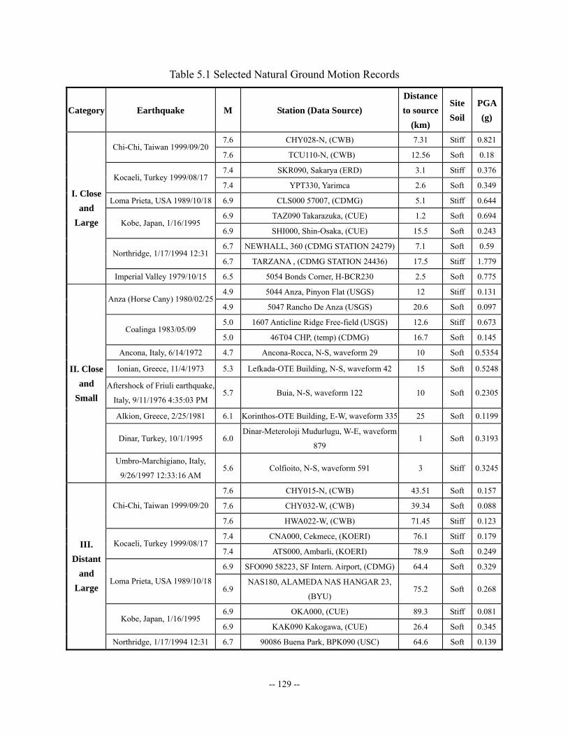
-- 129 --
Table 5.1 Selected Natural Ground Motion Records
Category Earthquake M Station (Data Source) Distance to source
(km)
Site Soil
PGA (g)
7.6 CHY028-N, (CWB) 7.31 Stiff 0.821 Chi-Chi, Taiwan 1999/09/20
7.6 TCU110-N, (CWB) 12.56 Soft 0.18
7.4 SKR090, Sakarya (ERD) 3.1 Stiff 0.376 Kocaeli, Turkey 1999/08/17
7.4 YPT330, Yarimca 2.6 Soft 0.349
Loma Prieta, USA 1989/10/18 6.9 CLS000 57007, (CDMG) 5.1 Stiff 0.644
6.9 TAZ090 Takarazuka, (CUE) 1.2 Soft 0.694 Kobe, Japan, 1/16/1995
6.9 SHI000, Shin-Osaka, (CUE) 15.5 Soft 0.243
6.7 NEWHALL, 360 (CDMG STATION 24279) 7.1 Soft 0.59 Northridge, 1/17/1994 12:31
6.7 TARZANA , (CDMG STATION 24436) 17.5 Stiff 1.779
I. Close and
Large
Imperial Valley 1979/10/15 6.5 5054 Bonds Corner, H-BCR230 2.5 Soft 0.775
4.9 5044 Anza, Pinyon Flat (USGS) 12 Stiff 0.131 Anza (Horse Cany) 1980/02/25
4.9 5047 Rancho De Anza (USGS) 20.6 Soft 0.097
5.0 1607 Anticline Ridge Free-field (USGS) 12.6 Stiff 0.673 Coalinga 1983/05/09
5.0 46T04 CHP, (temp) (CDMG) 16.7 Soft 0.145
Ancona, Italy, 6/14/1972 4.7 Ancona-Rocca, N-S, waveform 29 10 Soft 0.5354
Ionian, Greece, 11/4/1973 5.3 Lefkada-OTE Building, N-S, waveform 42 15 Soft 0.5248
Aftershock of Friuli earthquake,
Italy, 9/11/1976 4:35:03 PM 5.7 Buia, N-S, waveform 122 10 Soft 0.2305
Alkion, Greece, 2/25/1981 6.1 Korinthos-OTE Building, E-W, waveform 335 25 Soft 0.1199
Dinar, Turkey, 10/1/1995 6.0 Dinar-Meteroloji Mudurlugu, W-E, waveform
879 1 Soft 0.3193
II. Close and
Small
Umbro-Marchigiano, Italy,
9/26/1997 12:33:16 AM 5.6 Colfioito, N-S, waveform 591 3 Stiff 0.3245
7.6 CHY015-N, (CWB) 43.51 Soft 0.157
7.6 CHY032-W, (CWB) 39.34 Soft 0.088 Chi-Chi, Taiwan 1999/09/20
7.6 HWA022-W, (CWB) 71.45 Stiff 0.123
7.4 CNA000, Cekmece, (KOERI) 76.1 Stiff 0.179 Kocaeli, Turkey 1999/08/17
7.4 ATS000, Ambarli, (KOERI) 78.9 Soft 0.249
6.9 SFO090 58223, SF Intern. Airport, (CDMG) 64.4 Soft 0.329
Loma Prieta, USA 1989/10/18 6.9
NAS180, ALAMEDA NAS HANGAR 23,
(BYU) 75.2 Soft 0.268
6.9 OKA000, (CUE) 89.3 Stiff 0.081 Kobe, Japan, 1/16/1995
6.9 KAK090 Kakogawa, (CUE) 26.4 Soft 0.345
III. Distant
and Large
Northridge, 1/17/1994 12:31 6.7 90086 Buena Park, BPK090 (USC) 64.6 Soft 0.139
-- 130 --
5.2.2 Natural Ground Motions Applicability Evaluation
The 30 selected ground motion records were corrected and filtered from natural raw data. Even
though the selections account for basic features of earthquake strikes, their frequency contents
are investigated to ensure the frequency range is sufficiently wide to affect high-rise building
seismic behavior. The evaluations are performed using both response spectra and power spectra
for energy distribution over the frequency domain.
Source Data Correction and Filtering
Raw ground motion data from stations is not often used. Instead, the strong motion data is
processed in order to: (1) correct data by eliminating the effects of a moving recording
instrument, and (2) reduce random noise in the recorded signals. Due to technological
developments, most recent records are measured by digital instruments. Many old
accelerograms, such as some Category II records for earthquakes in the 1970’s and 80’s, are
analog records that must be digitized before processing. The basic processing steps for an
acceleration time series obtained by digitizing analog records or from digital instruments are:
• Baseline removal;
• Conditioning and padding the ends of the accelerograms;
• Acausal band pass filtering of the acceleration;
• Integration of corrected acceleration without decimation to velocity and displacement,
and
• Response spectra computation.
-- 131 --
Among the 30 ground motion records, 20 from Categories I and III are from U.S. sources, such
as the Pacific Earthquake Engineering Research Center (PEER) strong motion database. The
remaining records are from the European Strong Motion Database (by Ambraseys et al. (2004)).
PEER’s processing concentrates on extending the high and low frequency ranges of the usable
signals within the records on an individual component basis. More recent data, especially from
digital recorders, generally do not require additional processing and are deposited into the
database after review. It is apparent that there is diversity in the data processing and filtering due
to the different record instruments, data formats, processing institutes, and techniques. The
records from the European database contain strong motion records at permanent, ground level
recording stations located in Europe and the Mediterranean region. All uncorrected records have
been pre-processed to account for irregularities such as spurious large amplitudes or very high
frequency acceleration points, non-zero sloping or translated baselines, poor quality digitization,
zero or negative time steps, and duplicate records. The pre-processed records have been
subjected to a uniform correction procedure to reduce the low and high frequency noise levels.
Eighth-order elliptical bandpass filtering is applied in the procedure using a frequency range
between 0.25 Hz and 25Hz. Table 5.2 shows the effective period ranges [TL, TU] for the 30
ground motion records. The record names correspond to Table 5.1 and follow the same order.
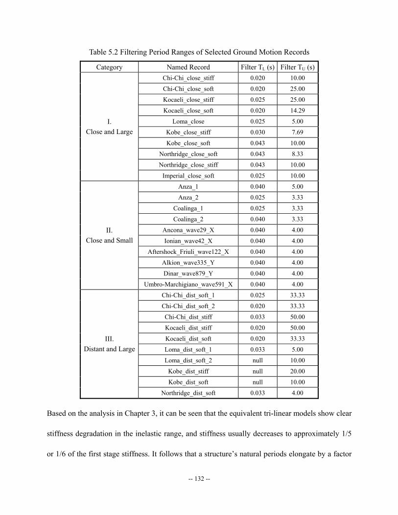
-- 132 --
Table 5.2 Filtering Period Ranges of Selected Ground Motion Records
Category Named Record Filter TL (s) Filter TU (s) Chi-Chi_close_stiff 0.020 10.00
Chi-Chi_close_soft 0.020 25.00
Kocaeli_close_stiff 0.025 25.00
Kocaeli_close_soft 0.020 14.29
Loma_close 0.025 5.00
Kobe_close_stiff 0.030 7.69
Kobe_close_soft 0.043 10.00
Northridge_close_soft 0.043 8.33
Northridge_close_stiff 0.043 10.00
I. Close and Large
Imperial_close_soft 0.025 10.00
Anza_1 0.040 5.00
Anza_2 0.025 3.33
Coalinga_1 0.025 3.33
Coalinga_2 0.040 3.33
Ancona_wave29_X 0.040 4.00
Ionian_wave42_X 0.040 4.00
Aftershock_Friuli_wave122_X 0.040 4.00
Alkion_wave335_Y 0.040 4.00
Dinar_wave879_Y 0.040 4.00
II. Close and Small
Umbro-Marchigiano_wave591_X 0.040 4.00
Chi-Chi_dist_soft_1 0.025 33.33
Chi-Chi_dist_soft_2 0.020 33.33
Chi-Chi_dist_stiff 0.033 50.00
Kocaeli_dist_stiff 0.020 50.00
Kocaeli_dist_soft 0.020 33.33
Loma_dist_soft_1 0.033 5.00
Loma_dist_soft_2 null 10.00
Kobe_dist_stiff null 20.00
Kobe_dist_soft null 10.00
III. Distant and Large
Northridge_dist_soft 0.033 4.00
Based on the analysis in Chapter 3, it can be seen that the equivalent tri-linear models show clear
stiffness degradation in the inelastic range, and stiffness usually decreases to approximately 1/5
or 1/6 of the first stage stiffness. It follows that a structure’s natural periods elongate by a factor

-- 133 --
of approximately 2.2 to 2.5 after yielding. After examining the selected ground motion records,
the following observations can be made:
• Categories I and III have a good frequency content distribution. Only ground motions one
and two do not satisfy the maximum inelastic period limit. Both categories are applicable
to the fragility assessment of all limit states for the reference structure.
• Category II exhibits generally low upper bounds for periods. This means the highly
inelastic responses of the reference building structure will be underestimated in some
cases. For this reason, the modeling of collapse prevention may not be as accurate as for
categories I and III.
Random Effects on Spectral Acceleration
The 30 selected ground motion records consist of wide ranges of three basic features: magnitude
(M), distance to source (D), and site condition (S). For further understanding of the effects of
uncertainty on the demand, it is necessary to evaluate the influences of these basic features of
ground motion records.
The basic dynamic natures of the ground motions are analyzed to provide the basis for further
comparisons of seismic demands. Figure 5.3 shows the elastic spectral acceleration diagrams
corresponding to the reference structure’s first four fundamental modes.
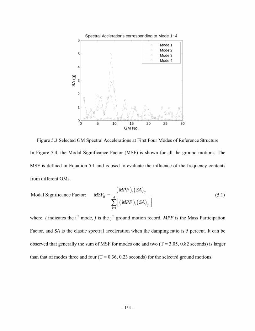
-- 134 --
0 5 10 15 20 25 300
1
2
3
4
5
6
GM No.
SA
(g)
Spectral Acclerations corresponding to Mode 1~4
Mode 1Mode 2Mode 3Mode 4
Figure 5.3 Selected GM Spectral Accelerations at First Four Modes of Reference Structure
In Figure 5.4, the Modal Significance Factor (MSF) is shown for all the ground motions. The
MSF is defined in Equation 5.1 and is used to evaluate the influence of the frequency contents
from different GMs.
( ) ( )
( ) ( )4
i=1
Modal Significance Factor: = i ijij
i ij
MPF SAMSF
MPF SA⎡ ⎤⎣ ⎦∑
(5.1)
where, i indicates the ith mode, j is the jth ground motion record, MPF is the Mass Participation
Factor, and SA is the elastic spectral acceleration when the damping ratio is 5 percent. It can be
observed that generally the sum of MSF for modes one and two (T = 3.05, 0.82 seconds) is larger
than that of modes three and four (T = 0.36, 0.23 seconds) for the selected ground motions.
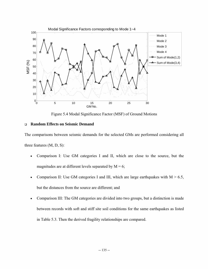
-- 135 --
0 5 10 15 20 25 300
10
20
30
40
50
60
70
80
90
100
GM No.
MS
F (%
)Modal Significance Factors corresponding to Mode 1~4
Mode 1
Mode 2
Mode 3
Mode 4
Sum of Mode(1,2)
Sum of Mode(3,4)
Figure 5.4 Modal Significance Factor (MSF) of Ground Motions
Random Effects on Seismic Demand
The comparisons between seismic demands for the selected GMs are performed considering all
three features (M, D, S):
• Comparison I: Use GM categories I and II, which are close to the source, but the
magnitudes are at different levels separated by M = 6;
• Comparison II: Use GM categories I and III, which are large earthquakes with M > 6.5,
but the distances from the source are different; and
• Comparison III: The GM categories are divided into two groups, but a distinction is made
between records with soft and stiff site soil conditions for the same earthquakes as listed
in Table 5.3. Then the derived fragility relationships are compared.

-- 136 --
Table 5.3 Earthquakes and Corresponding Ground Motion Records for Comparison III
Case No.
Earthquake M D (km) Station (Data Source) Site Soil
7.6 7.31 CHY028-N, (CWB) Stiff 1
Chi-Chi, Taiwan 1999/09/20 7.6 12.56 TCU110-N, (CWB) Soft
7.4 3.1 SKR090, Sakarya (ERD) Stiff 2
Kocaeli, Turkey 1999/08/17 7.4 2.6 YPT330, Yarimca Soft
6.7 7.1 NEWHALL, 360 (CDMG STATION 24279) Soft
3 Northridge,
1/17/1994 12:31 6.7 17.5 TARZANA-CEDAR HILL, (CDMG
STATION 24436) Stiff
4.9 12 5044 Anza, Pinyon Flat (USGS) Stiff 4
Anza (Horse Cany) 1980/02/25 4.9 20.6 5047 Rancho De Anza (USGS) Soft
5.0 12.6 1607 Anticline Ridge Free-field (USGS) Stiff 5
Coalinga 1983/05/09 5.0 16.7 46T04 CHP, (temp) (CDMG) Soft
7.6 43.51 CHY015-N, (CWB) Soft 6
Chi-Chi, Taiwan 1999/09/20 7.6 71.45 HWA022-W, (CWB) Stiff
7.4 76.1 CNA000, Cekmece, (KOERI) Stiff 7
Kocaeli, Turkey 1999/08/17 7.4 78.9 ATS000, Ambarli, (KOERI) Soft
6.9 89.3 OKA000, (CUE) Stiff 8
Kobe, Japan, 1/16/1995 6.9 26.4 KAK090 Kakogawa, (CUE) Soft
Figure 5.5 shows the variations in the extreme seismic demand (all GMs scaled to PGA=1.0g),
including maximum inter-story drift ratio (ISD) and inter-story pure translation ratio (ISPT),
caused by different ground motion features.
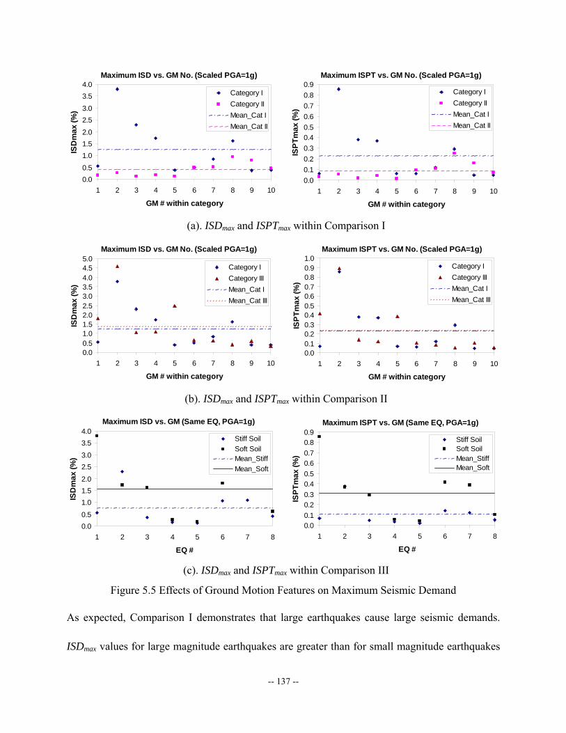
-- 137 --
Maximum ISD vs. GM No. (Scaled PGA=1g)
0.00.5
1.01.52.0
2.53.0
3.54.0
1 2 3 4 5 6 7 8 9 10
GM # within category
ISD
max
(%)
Category ICategory IIMean_Cat IMean_Cat II
Maximum ISPT vs. GM No. (Scaled PGA=1g)
0.00.10.20.30.40.50.60.70.80.9
1 2 3 4 5 6 7 8 9 10
GM # within category
ISPT
max
(%)
Category ICategory IIMean_Cat IMean_Cat II
(a). ISDmax and ISPTmax within Comparison I
Maximum ISD vs. GM No. (Scaled PGA=1g)
0.00.51.01.52.02.53.03.54.04.55.0
1 2 3 4 5 6 7 8 9 10
GM # within category
ISD
max
(%)
Category ICategory IIIMean_Cat IMean_Cat III
Maximum ISPT vs. GM No. (Scaled PGA=1g)
0.00.10.20.30.40.50.60.70.80.91.0
1 2 3 4 5 6 7 8 9 10
GM # within category
ISPT
max
(%)
Category ICategory IIIMean_Cat IMean_Cat III
(b). ISDmax and ISPTmax within Comparison II
Maximum ISD vs. GM (Same EQ, PGA=1g)
0.00.5
1.01.52.0
2.53.0
3.54.0
1 2 3 4 5 6 7 8
EQ #
ISD
max
(%)
Stiff SoilSoft SoilMean_StiffMean_Soft
Maximum ISPT vs. GM (Same EQ, PGA=1g)
0.00.10.20.30.40.50.60.70.80.9
1 2 3 4 5 6 7 8
EQ #
ISPT
max
(%)
Stiff SoilSoft SoilMean_StiffMean_Soft
(c). ISDmax and ISPTmax within Comparison III
Figure 5.5 Effects of Ground Motion Features on Maximum Seismic Demand
As expected, Comparison I demonstrates that large earthquakes cause large seismic demands.
ISDmax values for large magnitude earthquakes are greater than for small magnitude earthquakes
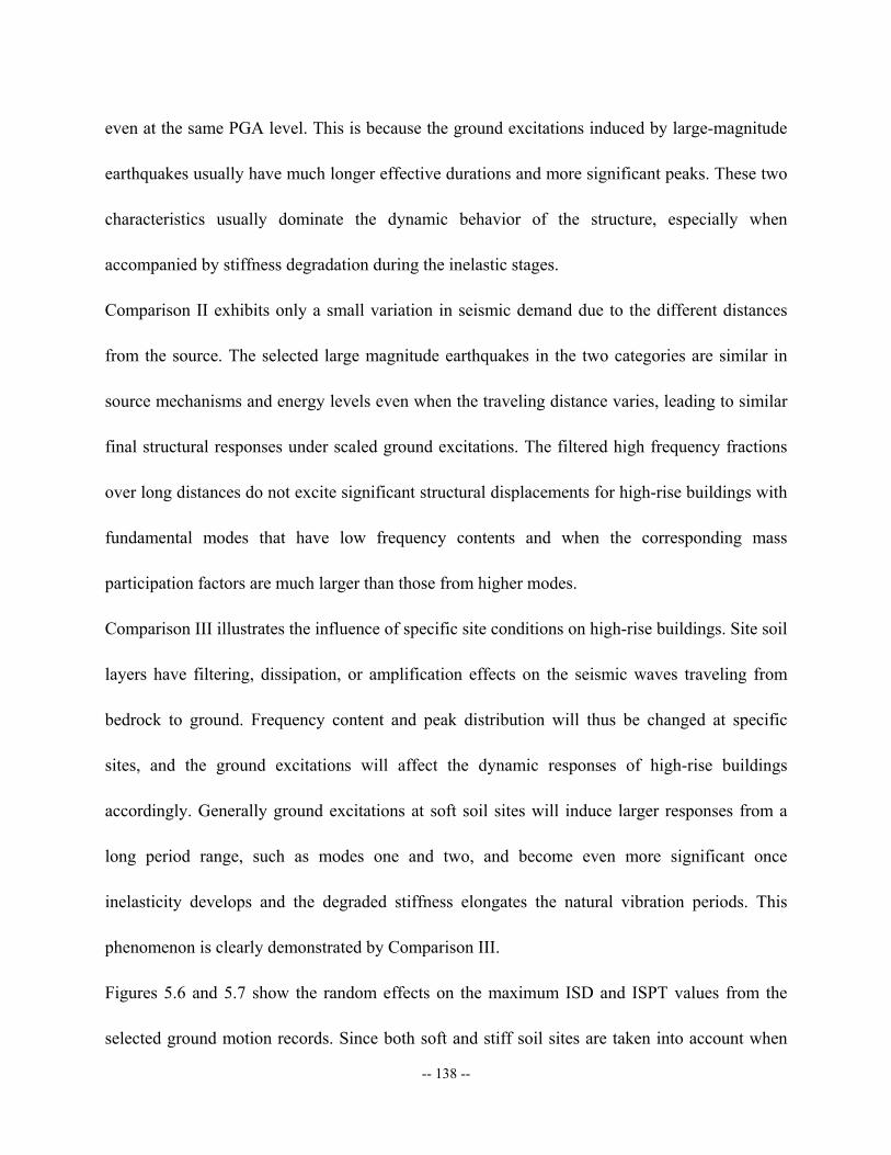
-- 138 --
even at the same PGA level. This is because the ground excitations induced by large-magnitude
earthquakes usually have much longer effective durations and more significant peaks. These two
characteristics usually dominate the dynamic behavior of the structure, especially when
accompanied by stiffness degradation during the inelastic stages.
Comparison II exhibits only a small variation in seismic demand due to the different distances
from the source. The selected large magnitude earthquakes in the two categories are similar in
source mechanisms and energy levels even when the traveling distance varies, leading to similar
final structural responses under scaled ground excitations. The filtered high frequency fractions
over long distances do not excite significant structural displacements for high-rise buildings with
fundamental modes that have low frequency contents and when the corresponding mass
participation factors are much larger than those from higher modes.
Comparison III illustrates the influence of specific site conditions on high-rise buildings. Site soil
layers have filtering, dissipation, or amplification effects on the seismic waves traveling from
bedrock to ground. Frequency content and peak distribution will thus be changed at specific
sites, and the ground excitations will affect the dynamic responses of high-rise buildings
accordingly. Generally ground excitations at soft soil sites will induce larger responses from a
long period range, such as modes one and two, and become even more significant once
inelasticity develops and the degraded stiffness elongates the natural vibration periods. This
phenomenon is clearly demonstrated by Comparison III.
Figures 5.6 and 5.7 show the random effects on the maximum ISD and ISPT values from the
selected ground motion records. Since both soft and stiff soil sites are taken into account when
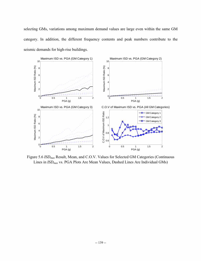
-- 139 --
selecting GMs, variations among maximum demand values are large even within the same GM
category. In addition, the different frequency contents and peak numbers contribute to the
seismic demands for high-rise buildings.
0 0.5 1 1.5 20
2
4
6
8
10
Max
imum
ISD
Rat
io (%
)
PGA (g)
Maximum ISD vs. PGA (GM Category 1)
0 0.5 1 1.5 20
2
4
6
8
10
Max
imum
ISD
Rat
io (%
)PGA (g)
Maximum ISD vs. PGA (GM Category 2)
0 0.5 1 1.5 20
2
4
6
8
10
Max
imum
ISD
Rat
io (%
)
PGA (g)
Maximum ISD vs. PGA (GM Category 3)
0 0.5 1 1.5 2
0.6
0.8
1
1.2
C.O
.V o
f Max
imum
ISD
Rat
io
PGA (g)
C.O.V of Maximum ISD vs. PGA (All GM Categories)
GM Category 1
GM Category 2
GM Category 3
Figure 5.6 ISDmax Result, Mean, and C.O.V. Values for Selected GM Categories (Continuous Lines in ISDmax vs. PGA Plots Are Mean Values, Dashed Lines Are Individual GMs)

-- 140 --
0 0.5 1 1.5 20
0.5
1
1.5
2
Max
imum
ISP
T R
atio
(%)
PGA (g)
Maximum ISPT vs. PGA (GM Category 1)
0 0.5 1 1.5 20
0.5
1
1.5
2
Max
imum
ISP
T R
atio
(%)
PGA (g)
Maximum ISPT vs. PGA (GM Category 2)
0 0.5 1 1.5 20
0.5
1
1.5
2
Max
imum
ISP
T R
atio
(%)
PGA (g)
Maximum ISPT vs. PGA (GM Category 3)
0 0.5 1 1.5 2
0.6
0.8
1
1.2
C.O
.V o
f Max
imum
ISP
T R
atio
PGA (g)
C.O.V of Maximum ISPT vs. PGA (All GM Categories)
GM Category 1GM Category 2GM Category 3
Figure 5.7 ISPTmax Result, Mean, and C.O.V. Values for Selected GM Categories (Continuous Lines in ISPTmax vs. PGA Plots Are Mean Values, Dashed Lines Are Individual GMs)
An important observation is that the ground motion sets significantly influence the seismic
demand of high-rise buildings, and hence greatly affect the fragility relationship assessment.
Random Effects on Fourier and Power Spectra
To gain further insight into the frequency contents and energy distributions, Fourier amplitudes
and power spectra densities were computed for all selected natural ground motion records over
the frequency domain. They are normalized and plotted separately for each GM category in
Figures 5.8 through 5.10. The most influential period range is related to the reference structure’s
elastic and inelastic natural modal periods, and in this case the range between 0.1 and 10 seconds
is of interest.
-- 141 --
10-1 100 1010
0.1
0.2
0.3
0.4
0.5
0.6
0.7
0.8
0.9
1Fourier Amplitude of Natural Record Category 1
Natural Period T (sec)
Four
ier A
mpl
itude
10-1 100 101
0
0.1
0.2
0.3
0.4
0.5
0.6
0.7
0.8
0.9
1Power Spectral Density of Natural Record Category 1
Natural Period T (sec)
Pow
er S
pect
ral D
ensi
ty
Figure 5.8 Fourier and Power Spectra of Category I
10-1 100 1010
0.1
0.2
0.3
0.4
0.5
0.6
0.7
0.8
0.9
1Fourier Amplitude of Natural Record Category 2
Natural Period T (sec)
Four
ier A
mpl
itude
10-1 100 101
0
0.1
0.2
0.3
0.4
0.5
0.6
0.7
0.8
0.9
1Power Spectral Density of Natural Record Category 2
Natural Period T (sec)
Pow
er S
pect
ral D
ensi
ty
Figure 5.9 Fourier and Power Spectra of Category II
10-1 100 1010
0.1
0.2
0.3
0.4
0.5
0.6
0.7
0.8
0.9
1Fourier Amplitude of Natural Record Category 3
Natural Period T (sec)
Four
ier A
mpl
itude
10-1 100 101
0
0.1
0.2
0.3
0.4
0.5
0.6
0.7
0.8
0.9
1Power Spectral Density of Natural Record Category 3
Natural Period T (sec)
Pow
er S
pect
ral D
ensi
ty
Figure 5.10 Fourier and Power Spectra of Category III
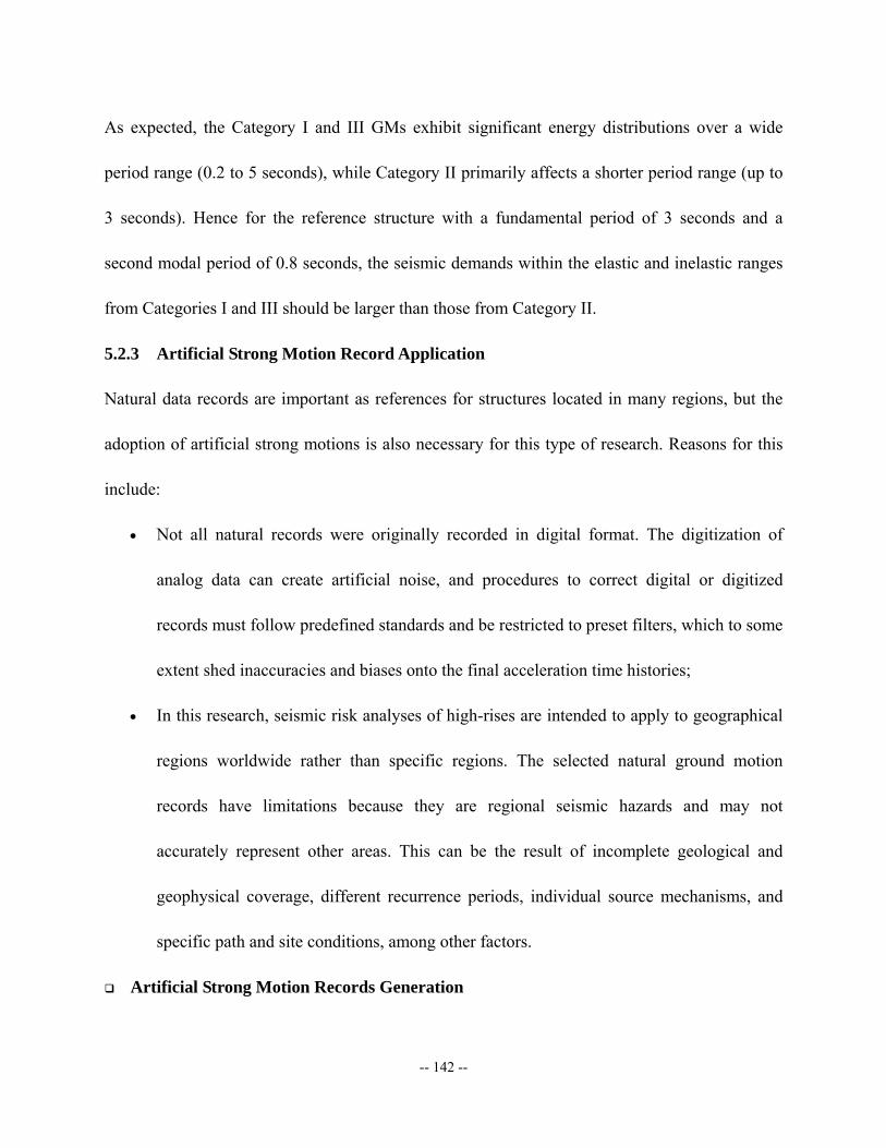
-- 142 --
As expected, the Category I and III GMs exhibit significant energy distributions over a wide
period range (0.2 to 5 seconds), while Category II primarily affects a shorter period range (up to
3 seconds). Hence for the reference structure with a fundamental period of 3 seconds and a
second modal period of 0.8 seconds, the seismic demands within the elastic and inelastic ranges
from Categories I and III should be larger than those from Category II.
5.2.3 Artificial Strong Motion Record Application
Natural data records are important as references for structures located in many regions, but the
adoption of artificial strong motions is also necessary for this type of research. Reasons for this
include:
• Not all natural records were originally recorded in digital format. The digitization of
analog data can create artificial noise, and procedures to correct digital or digitized
records must follow predefined standards and be restricted to preset filters, which to some
extent shed inaccuracies and biases onto the final acceleration time histories;
• In this research, seismic risk analyses of high-rises are intended to apply to geographical
regions worldwide rather than specific regions. The selected natural ground motion
records have limitations because they are regional seismic hazards and may not
accurately represent other areas. This can be the result of incomplete geological and
geophysical coverage, different recurrence periods, individual source mechanisms, and
specific path and site conditions, among other factors.
Artificial Strong Motion Records Generation
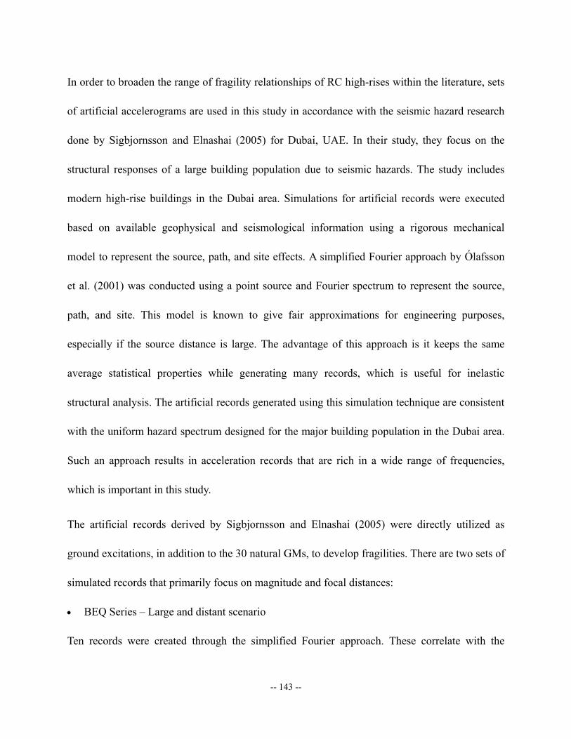
-- 143 --
In order to broaden the range of fragility relationships of RC high-rises within the literature, sets
of artificial accelerograms are used in this study in accordance with the seismic hazard research
done by Sigbjornsson and Elnashai (2005) for Dubai, UAE. In their study, they focus on the
structural responses of a large building population due to seismic hazards. The study includes
modern high-rise buildings in the Dubai area. Simulations for artificial records were executed
based on available geophysical and seismological information using a rigorous mechanical
model to represent the source, path, and site effects. A simplified Fourier approach by Ólafsson
et al. (2001) was conducted using a point source and Fourier spectrum to represent the source,
path, and site. This model is known to give fair approximations for engineering purposes,
especially if the source distance is large. The advantage of this approach is it keeps the same
average statistical properties while generating many records, which is useful for inelastic
structural analysis. The artificial records generated using this simulation technique are consistent
with the uniform hazard spectrum designed for the major building population in the Dubai area.
Such an approach results in acceleration records that are rich in a wide range of frequencies,
which is important in this study.
The artificial records derived by Sigbjornsson and Elnashai (2005) were directly utilized as
ground excitations, in addition to the 30 natural GMs, to develop fragilities. There are two sets of
simulated records that primarily focus on magnitude and focal distances:
• BEQ Series – Large and distant scenario
Ten records were created through the simplified Fourier approach. These correlate with the

-- 144 --
response spectra of large, distant earthquakes and exhibit a relatively low response for stiff
structures, an increased response for long period structures, and the apparent intermediate period
gap. All the synthetic records were simulated independently, and each one should be regarded as
a sample of many possibilities. Figure 5.11 shows three sample records from this category.
0 10 20 30 40 50 60-0.2
-0.1
0
0.1
0.2Accelerogram corresponding to BEQTS03
Acc
eler
atio
n (g
)
0 10 20 30 40 50 60-0.2
-0.1
0
0.1
0.2Accelerogram corresponding to BEQTS06
Acc
eler
atio
n (g
)
0 10 20 30 40 50 60-0.2
-0.1
0
0.1
0.2Accelerogram corresponding to BEQTS09
Time (sec)
Acc
eler
atio
n (g
)
Figure 5.11 Three Artificial Accelerograms Samples from BEQ Series
• SEQ Series – Moderate and close scenario
Ten records were created through the simplified Fourier approach. These correlate with the
response spectra of small, close earthquakes, which tend to excite the higher modes of high-rise
building structures. As with the BEQ series, all the synthetic records are simulated independently.
Figure 5.12 shows three sample records from this category.
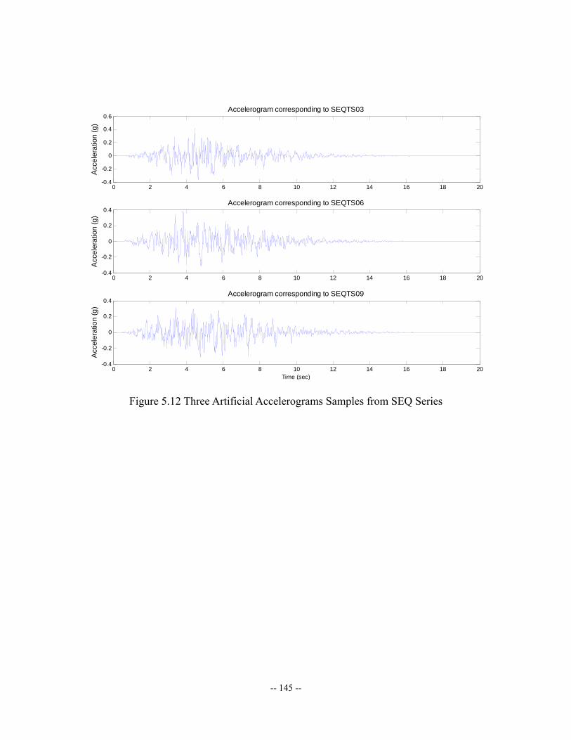
-- 145 --
0 2 4 6 8 10 12 14 16 18 20-0.4
-0.2
0
0.2
0.4
0.6Accelerogram corresponding to SEQTS03
Acc
eler
atio
n (g
)
0 2 4 6 8 10 12 14 16 18 20-0.4
-0.2
0
0.2
0.4Accelerogram corresponding to SEQTS06
Acc
eler
atio
n (g
)
0 2 4 6 8 10 12 14 16 18 20-0.4
-0.2
0
0.2
0.4Accelerogram corresponding to SEQTS09
Time (sec)
Acc
eler
atio
n (g
)
Figure 5.12 Three Artificial Accelerograms Samples from SEQ Series

-- 146 --
The detail information of these two artificial record series is listed in Table 5.4.
Table 5.4 Artificial Strong Motion Record Details
Earthquake Scenario M D (km) Record Name PGA (g) BEQTS01 0.1246 BEQTS02 0.1108 BEQTS03 0.1150 BEQTS04 0.1331 BEQTS05 0.1475 BEQTS06 0.1371 BEQTS07 0.1392 BEQTS08 0.1610 BEQTS09 0.1207
Distant and Large 7.4 100
BEQTS010 0.1227 SEQTS01 0.3413 SEQTS02 0.3398 SEQTS03 0.4144 SEQTS04 0.3609 SEQTS05 0.3839 SEQTS06 0.3784 SEQTS07 0.4432 SEQTS08 0.2707 SEQTS09 0.3144
Close and Small 6.0 10
SEQTS010 0.3398
Random Effects on Fourier and Power Spectra
Using the same concepts and methodologies, energy distribution is analyzed for the artificial
ground motion records over frequency domain. They are also normalized and plotted separately
for BEQ and SEQ series as following Figures 5.13 and 5.14, and the interested period range is
again set here within [0.1, 10] seconds.
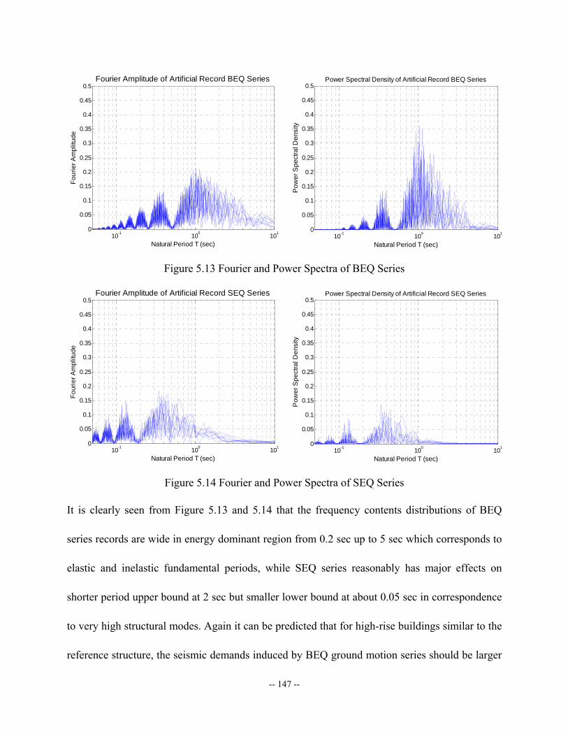
-- 147 --
10-1 100 1010
0.05
0.1
0.15
0.2
0.25
0.3
0.35
0.4
0.45
0.5Fourier Amplitude of Artificial Record BEQ Series
Natural Period T (sec)
Four
ier A
mpl
itude
10-1 100 101
0
0.05
0.1
0.15
0.2
0.25
0.3
0.35
0.4
0.45
0.5Power Spectral Density of Artificial Record BEQ Series
Natural Period T (sec)
Pow
er S
pect
ral D
ensi
ty
Figure 5.13 Fourier and Power Spectra of BEQ Series
10-1 100 1010
0.05
0.1
0.15
0.2
0.25
0.3
0.35
0.4
0.45
0.5Fourier Amplitude of Artificial Record SEQ Series
Natural Period T (sec)
Four
ier A
mpl
itude
10-1 100 101
0
0.05
0.1
0.15
0.2
0.25
0.3
0.35
0.4
0.45
0.5Power Spectral Density of Artificial Record SEQ Series
Natural Period T (sec)
Pow
er S
pect
ral D
ensi
ty
Figure 5.14 Fourier and Power Spectra of SEQ Series
It is clearly seen from Figure 5.13 and 5.14 that the frequency contents distributions of BEQ
series records are wide in energy dominant region from 0.2 sec up to 5 sec which corresponds to
elastic and inelastic fundamental periods, while SEQ series reasonably has major effects on
shorter period upper bound at 2 sec but smaller lower bound at about 0.05 sec in correspondence
to very high structural modes. Again it can be predicted that for high-rise buildings similar to the
reference structure, the seismic demands induced by BEQ ground motion series should be larger
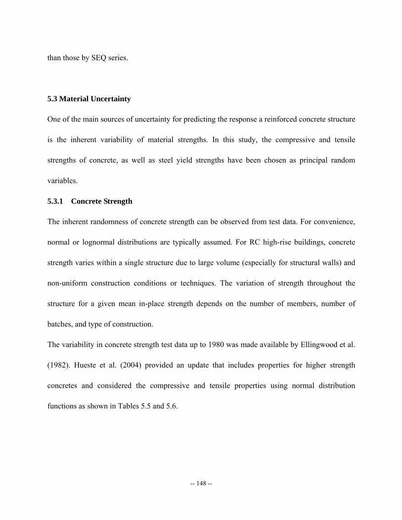
-- 148 --
than those by SEQ series.
5.3 Material Uncertainty
One of the main sources of uncertainty for predicting the response a reinforced concrete structure
is the inherent variability of material strengths. In this study, the compressive and tensile
strengths of concrete, as well as steel yield strengths have been chosen as principal random
variables.
5.3.1 Concrete Strength
The inherent randomness of concrete strength can be observed from test data. For convenience,
normal or lognormal distributions are typically assumed. For RC high-rise buildings, concrete
strength varies within a single structure due to large volume (especially for structural walls) and
non-uniform construction conditions or techniques. The variation of strength throughout the
structure for a given mean in-place strength depends on the number of members, number of
batches, and type of construction.
The variability in concrete strength test data up to 1980 was made available by Ellingwood et al.
(1982). Hueste et al. (2004) provided an update that includes properties for higher strength
concretes and considered the compressive and tensile properties using normal distribution
functions as shown in Tables 5.5 and 5.6.
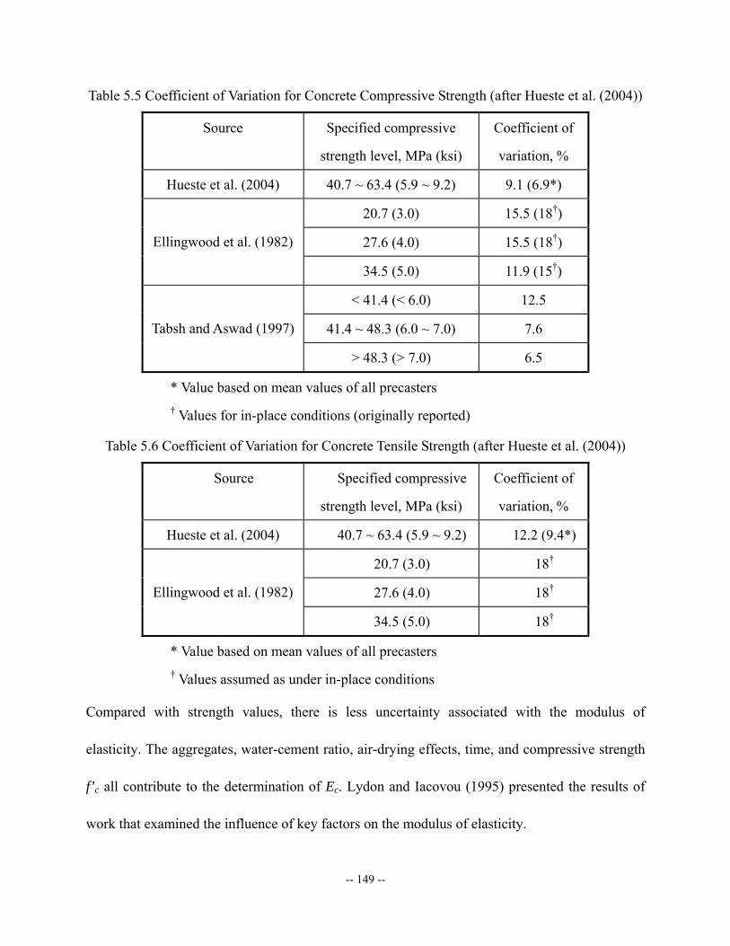
-- 149 --
Table 5.5 Coefficient of Variation for Concrete Compressive Strength (after Hueste et al. (2004))
Source Specified compressive
strength level, MPa (ksi)
Coefficient of
variation, %
Hueste et al. (2004) 40.7 ~ 63.4 (5.9 ~ 9.2) 9.1 (6.9*)
20.7 (3.0) 15.5 (18†)
27.6 (4.0) 15.5 (18†) Ellingwood et al. (1982)
34.5 (5.0) 11.9 (15†)
< 41.4 (< 6.0) 12.5
41.4 ~ 48.3 (6.0 ~ 7.0) 7.6 Tabsh and Aswad (1997)
> 48.3 (> 7.0) 6.5
* Value based on mean values of all precasters † Values for in-place conditions (originally reported)
Table 5.6 Coefficient of Variation for Concrete Tensile Strength (after Hueste et al. (2004))
Source Specified compressive
strength level, MPa (ksi)
Coefficient of
variation, %
Hueste et al. (2004) 40.7 ~ 63.4 (5.9 ~ 9.2) 12.2 (9.4*)
20.7 (3.0) 18†
27.6 (4.0) 18† Ellingwood et al. (1982)
34.5 (5.0) 18†
* Value based on mean values of all precasters † Values assumed as under in-place conditions
Compared with strength values, there is less uncertainty associated with the modulus of
elasticity. The aggregates, water-cement ratio, air-drying effects, time, and compressive strength
f’c all contribute to the determination of Ec. Lydon and Iacovou (1995) presented the results of
work that examined the influence of key factors on the modulus of elasticity.
-- 150 --
5.3.2 Steel Strength
Mirza and MacGregor (1979) reported results of approximately 4000 tests on Grade 40 and 60
steel reinforcing bars. The results from these tests were examined to obtain statistical
relationships for various mechanical properties. The sample included No. 3 through No. 18 sizes
of Grades 40 and 60 reinforcements. The means and coefficients of variation of the mill test
yield strengths were found to be 48.8 ksi (337 MPa) and 10.7% for Grade 40 and 71 ksi (490
MPa) and 9.3% for Grade 60 bars. Beta distributions were used to represent both of these sets of
data. The static yield strength was found to be 3.5 ksi (24 MPa)) lower on average than the mill
test yield strength in both cases, with a coefficient of variation of 13.4%.
Bournonville et al. (2004) assessed the variability of the mechanical properties and weight of
steel reinforcing bars produced by more than 34 mills in the United States and Canada under
ASTM A615, A616, and A706 in 1997. Using a similar approach to that of Mirza and
MacGregor (1979), beta functions were obtained from parametric studies to represent the yield
and tensile (ultimate) strength distributions for different bar sizes, grades, and steel types. After
comparing the test data with previous findings, Bournonville et al. (2004) concluded that:
• The beta distributions for yield strengths covering all A615 Grade 40 and all A615 Grade
60 bars provide good representations for the distributions for individual bar sizes within
each of these grades, with the exception of A615 No. 14 and No. 18 bars, which exhibit
significantly different distribution functions. This is illustrated in Figure 5.15.
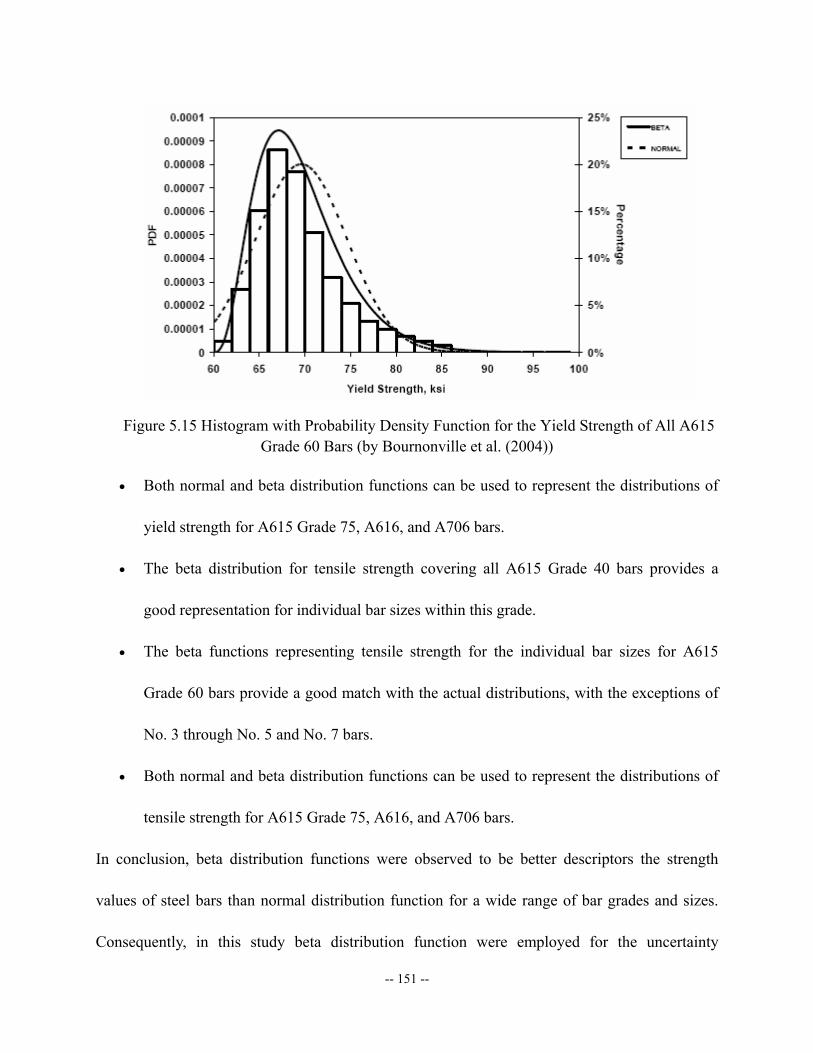
-- 151 --
Figure 5.15 Histogram with Probability Density Function for the Yield Strength of All A615 Grade 60 Bars (by Bournonville et al. (2004))
• Both normal and beta distribution functions can be used to represent the distributions of
yield strength for A615 Grade 75, A616, and A706 bars.
• The beta distribution for tensile strength covering all A615 Grade 40 bars provides a
good representation for individual bar sizes within this grade.
• The beta functions representing tensile strength for the individual bar sizes for A615
Grade 60 bars provide a good match with the actual distributions, with the exceptions of
No. 3 through No. 5 and No. 7 bars.
• Both normal and beta distribution functions can be used to represent the distributions of
tensile strength for A615 Grade 75, A616, and A706 bars.
In conclusion, beta distribution functions were observed to be better descriptors the strength
values of steel bars than normal distribution function for a wide range of bar grades and sizes.
Consequently, in this study beta distribution function were employed for the uncertainty
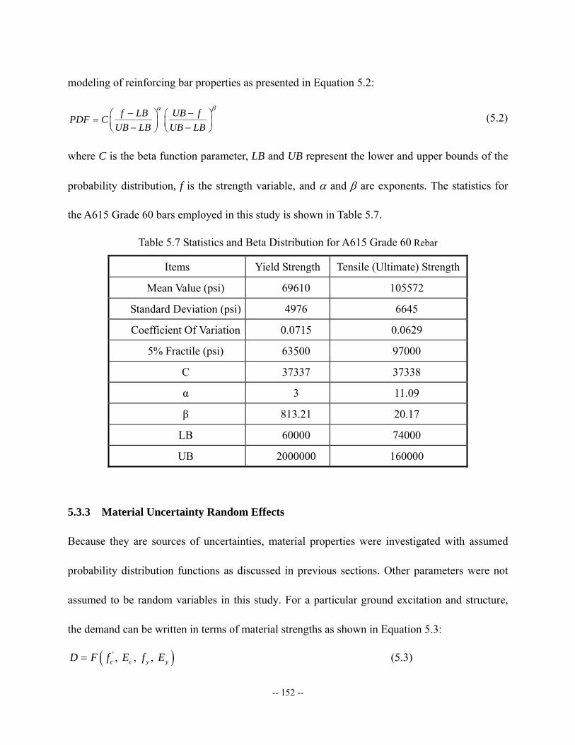
-- 152 --
modeling of reinforcing bar properties as presented in Equation 5.2:
f LB UB fPDF CUB LB UB LB
α β− −⎛ ⎞ ⎛ ⎞= ⎜ ⎟ ⎜ ⎟− −⎝ ⎠ ⎝ ⎠ (5.2)
where C is the beta function parameter, LB and UB represent the lower and upper bounds of the
probability distribution, f is the strength variable, and α and β are exponents. The statistics for
the A615 Grade 60 bars employed in this study is shown in Table 5.7.
Table 5.7 Statistics and Beta Distribution for A615 Grade 60 Rebar
Items Yield Strength Tensile (Ultimate) Strength
Mean Value (psi) 69610 105572
Standard Deviation (psi) 4976 6645
Coefficient Of Variation 0.0715 0.0629
5% Fractile (psi) 63500 97000
C 37337 37338
α 3 11.09
β 813.21 20.17
LB 60000 74000
UB 2000000 160000
5.3.3 Material Uncertainty Random Effects
Because they are sources of uncertainties, material properties were investigated with assumed
probability distribution functions as discussed in previous sections. Other parameters were not
assumed to be random variables in this study. For a particular ground excitation and structure,
the demand can be written in terms of material strengths as shown in Equation 5.3:
( )' , , , c c y yD F f E f E= (5.3)
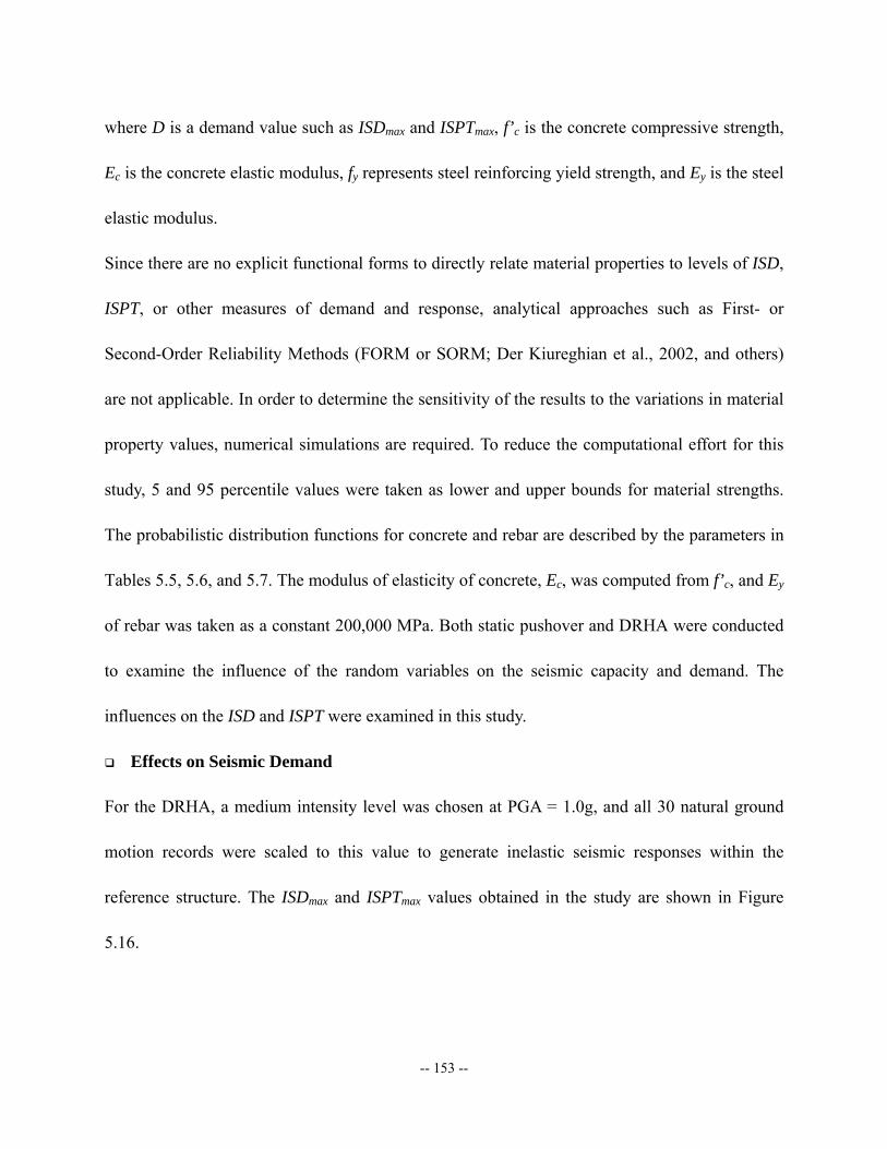
-- 153 --
where D is a demand value such as ISDmax and ISPTmax, f’c is the concrete compressive strength,
Ec is the concrete elastic modulus, fy represents steel reinforcing yield strength, and Ey is the steel
elastic modulus.
Since there are no explicit functional forms to directly relate material properties to levels of ISD,
ISPT, or other measures of demand and response, analytical approaches such as First- or
Second-Order Reliability Methods (FORM or SORM; Der Kiureghian et al., 2002, and others)
are not applicable. In order to determine the sensitivity of the results to the variations in material
property values, numerical simulations are required. To reduce the computational effort for this
study, 5 and 95 percentile values were taken as lower and upper bounds for material strengths.
The probabilistic distribution functions for concrete and rebar are described by the parameters in
Tables 5.5, 5.6, and 5.7. The modulus of elasticity of concrete, Ec, was computed from f’c, and Ey
of rebar was taken as a constant 200,000 MPa. Both static pushover and DRHA were conducted
to examine the influence of the random variables on the seismic capacity and demand. The
influences on the ISD and ISPT were examined in this study.
Effects on Seismic Demand
For the DRHA, a medium intensity level was chosen at PGA = 1.0g, and all 30 natural ground
motion records were scaled to this value to generate inelastic seismic responses within the
reference structure. The ISDmax and ISPTmax values obtained in the study are shown in Figure
5.16.
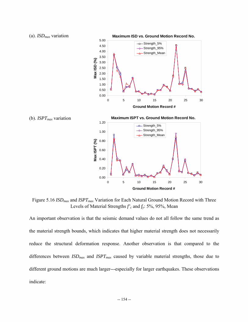
-- 154 --
(a). ISDmax variation Maximum ISD vs. Ground Motion Record No.
0.00
0.50
1.00
1.50
2.00
2.50
3.00
3.50
4.00
4.50
5.00
0 5 10 15 20 25 30
Ground Motion Record #
Max
ISD
(%)
Strength_5%Strength_95%Strength_Mean
(b). ISPTmax variation Maximum ISPT vs. Ground Motion Record No.
0.00
0.20
0.40
0.60
0.80
1.00
1.20
0 5 10 15 20 25 30
Ground Motion Record #
Max
ISPT
(%)
Strength_5%Strength_95%Strength_Mean
Figure 5.16 ISDmax and ISPTmax Variation for Each Natural Ground Motion Record with Three Levels of Material Strengths f’c and fy: 5%, 95%, Mean
An important observation is that the seismic demand values do not all follow the same trend as
the material strength bounds, which indicates that higher material strength does not necessarily
reduce the structural deformation response. Another observation is that compared to the
differences between ISDmax and ISPTmax caused by variable material strengths, those due to
different ground motions are much larger---especially for larger earthquakes. These observations
indicate:
-- 155 --
• Dynamic response uncertainties are dominated by the random nature of the ground
excitation for high-rise building structures; and
• The seismic deformation demand is primarily influenced by structural stiffness rather
than strength because the former affects the vibration period.
A statistical analysis of these results was performed to evaluate the probabilistic features of
ISDmax and ISPTmax for each ground motion record. A normal distribution of results was assumed
to evaluate the coefficient of variation. The relative deviations were calculated using regression
analyses as demonstrated in Figure 5.17 and Equation 5.4. The C.O.V. values were found to be
less than 10% on average and less than 20% for extreme cases, as Figure 5.18 shows.
(Assumed Normal here)
Ground Motion Set #
Dmax
i
Dmax
Probabilistic Distributionby Material Uncertainties
Figure 5.17 Variation of Maximum Demand Values due to Material Uncertainties 2
21 , , 1 ~ 302
i i
i
X
ii i
ii
p e iμσ σ
δμσ π
⎛ ⎞−−⎜ ⎟⎜ ⎟⎝ ⎠= = = (5.4)
where, Probability density function of seismic demand at ith ground motion record
Normal distribution mean value at ith ground motion record
Normal distribution standard d
i
i
i
p
μ
σ
−
−
− eviation at ith ground motion record
Normal distribution C.O.V at ith ground motion recordiδ −
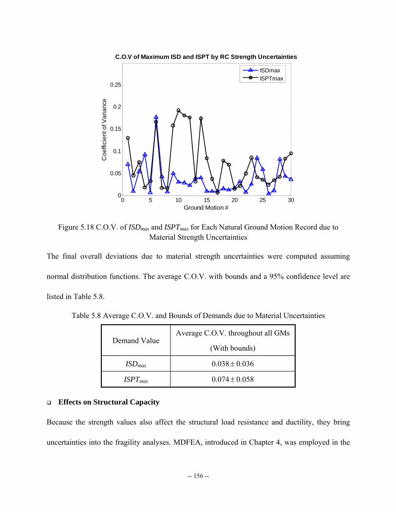
-- 156 --
0 5 10 15 20 25 300
0.05
0.1
0.15
0.2
0.25
Coe
ffici
ent o
f Var
ianc
e
Ground Motion #
C.O.V of Maximum ISD and ISPT by RC Strength Uncertainties
ISDmaxISPTmax
Figure 5.18 C.O.V. of ISDmax and ISPTmax for Each Natural Ground Motion Record due to Material Strength Uncertainties
The final overall deviations due to material strength uncertainties were computed assuming
normal distribution functions. The average C.O.V. with bounds and a 95% confidence level are
listed in Table 5.8.
Table 5.8 Average C.O.V. and Bounds of Demands due to Material Uncertainties
Demand Value Average C.O.V. throughout all GMs
(With bounds)
ISDmax 0.038± 0.036
ISPTmax 0.074± 0.058
Effects on Structural Capacity
Because the strength values also affect the structural load resistance and ductility, they bring
uncertainties into the fragility analyses. MDFEA, introduced in Chapter 4, was employed in the
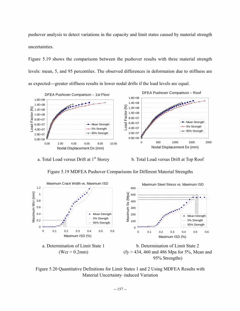
-- 157 --
pushover analysis to detect variations in the capacity and limit states caused by material strength
uncertainties.
Figure 5.19 shows the comparisons between the pushover results with three material strength
levels: mean, 5, and 95 percentiles. The observed differences in deformation due to stiffness are
as expected---greater stiffness results in lower nodal drifts if the load levels are equal.
DFEA Pushover Comparison -- 1st Floor
0.0E+00
2.0E+07
4.0E+07
6.0E+07
8.0E+07
1.0E+08
1.2E+08
1.4E+08
1.6E+08
0.00 2.00 4.00 6.00 8.00 10.00
Nodal Displacement Dx (mm)
Load
Fac
tor (
N)
Mean Strength5% Strength95% Strength
DFEA Pushover Comparison -- Roof
0.0E+00
2.0E+07
4.0E+07
6.0E+07
8.0E+07
1.0E+08
1.2E+08
1.4E+08
1.6E+08
0 500 1000 1500 2000
Nodal Displacement Dx (mm)
Load
Fac
tor (
N)
Mean Strength5% Strength95% Strength
a. Total Load versus Drift at 1st Storey b. Total Load versus Drift at Top Roof
Figure 5.19 MDFEA Pushover Comparisons for Different Material Strengths
Maximum Crack Width vs. Maximum ISD
0
0.2
0.4
0.6
0.8
1
1.2
0 0.1 0.2 0.3 0.4 0.5 0.6
Maximum ISD (%)
Max
imum
Wcr
(mm
)
Mean Strength5% Strength95% Strength
Maximum Steel Stress vs. Maximum ISD
0
100
200
300
400
500
600
0 0.1 0.2 0.3 0.4 0.5 0.6
Maximum ISD (%)
Max
imum
Ss
(Mpa
)
Mean Strength5% Strength95% Strength
a. Determination of Limit State 1 (Wcr > 0.2mm)
b. Determination of Limit State 2 (fy > 434, 460 and 486 Mpa for 5%, Mean and
95% Strengths)
Figure 5.20 Quantitative Definitions for Limit States 1 and 2 Using MDFEA Results with Material Uncertainty–induced Variation
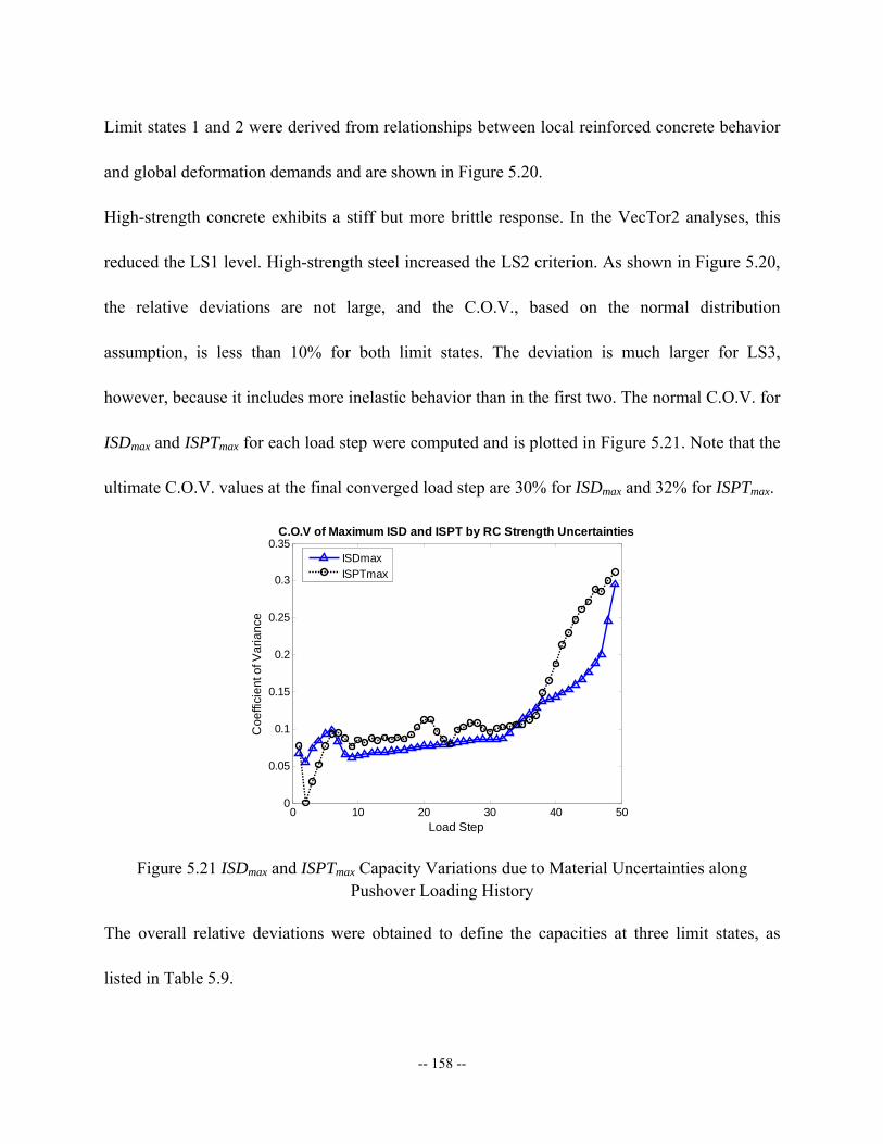
-- 158 --
Limit states 1 and 2 were derived from relationships between local reinforced concrete behavior
and global deformation demands and are shown in Figure 5.20.
High-strength concrete exhibits a stiff but more brittle response. In the VecTor2 analyses, this
reduced the LS1 level. High-strength steel increased the LS2 criterion. As shown in Figure 5.20,
the relative deviations are not large, and the C.O.V., based on the normal distribution
assumption, is less than 10% for both limit states. The deviation is much larger for LS3,
however, because it includes more inelastic behavior than in the first two. The normal C.O.V. for
ISDmax and ISPTmax for each load step were computed and is plotted in Figure 5.21. Note that the
ultimate C.O.V. values at the final converged load step are 30% for ISDmax and 32% for ISPTmax.
0 10 20 30 40 500
0.05
0.1
0.15
0.2
0.25
0.3
0.35
Coe
ffici
ent o
f Var
ianc
e
Load Step
C.O.V of Maximum ISD and ISPT by RC Strength Uncertainties
ISDmaxISPTmax
Figure 5.21 ISDmax and ISPTmax Capacity Variations due to Material Uncertainties along Pushover Loading History
The overall relative deviations were obtained to define the capacities at three limit states, as
listed in Table 5.9.
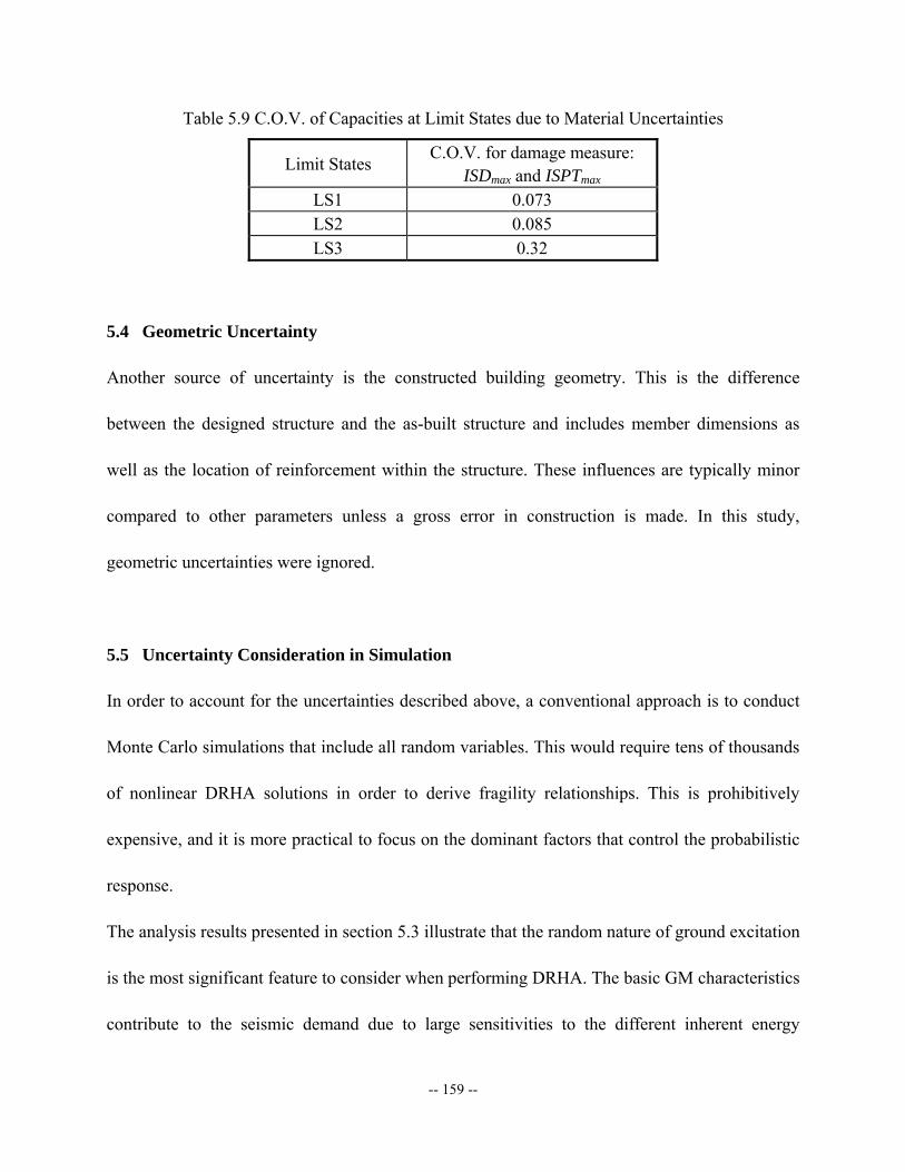
-- 159 --
Table 5.9 C.O.V. of Capacities at Limit States due to Material Uncertainties
Limit States C.O.V. for damage measure: ISDmax and ISPTmax
LS1 0.073 LS2 0.085 LS3 0.32
5.4 Geometric Uncertainty
Another source of uncertainty is the constructed building geometry. This is the difference
between the designed structure and the as-built structure and includes member dimensions as
well as the location of reinforcement within the structure. These influences are typically minor
compared to other parameters unless a gross error in construction is made. In this study,
geometric uncertainties were ignored.
5.5 Uncertainty Consideration in Simulation
In order to account for the uncertainties described above, a conventional approach is to conduct
Monte Carlo simulations that include all random variables. This would require tens of thousands
of nonlinear DRHA solutions in order to derive fragility relationships. This is prohibitively
expensive, and it is more practical to focus on the dominant factors that control the probabilistic
response.
The analysis results presented in section 5.3 illustrate that the random nature of ground excitation
is the most significant feature to consider when performing DRHA. The basic GM characteristics
contribute to the seismic demand due to large sensitivities to the different inherent energy

-- 160 --
distributions and frequency contents. Material uncertainties can be taken into account as
additional epistemic uncertainty in fragility relationships using statistical confidence levels, such
as 5 and 95 percentile bounds.
-- 161 --
6. Fragility Curve Assessment
6.1 Literature Survey
6.1.1 Existing Fragility Curves
Fragility curves are defined as the relationship between the conditional probability of reaching or
exceeding a certain damage states given the intensity measure of ground motion. Fragilitiy is
influenced by the nature of ground excitation, structure characteristics and the simulation
environment. The latter component comprises selection of structural model, limit states
definition and analysis platform. There are several proposed fragility relationships for different
reinforced concrete structural systems, using a variety of methodologies and parameters for
representation of seismic demand and damages. Rossetto and Elnashai (2003) classified the
existing fragility curves into four generic groups:
• Empirical Fragility Curves. These are derived through statistical analysis of real buildings
in past earthquakes. Examples of such fragilities are those proposed by Miyakoshi et al.
(1997), Orsini (1999) and Yamazaki and Murao (2000).
• Analytical Fragility Curves. This approach uses numerical techniques to simulate the
behavior of systems including variation of structural capacity and seismic demands.
Studies done in this category include: Singhal and Kiremidjian (1997) that has some
considerations for high-rise buildings, and Mosalem et al. (1997).
• Judgmental Fragility Curves. These are fragility curves that are based partially or wholly
on expert opinion. An example of these fragility curves are those implemented in
-- 162 --
HAZUS (reference to FEMA). The main advantage of this approach is that a wide range
of structure types are dealt with in the same manner hence the level of uncertainty,
though unknown, is uniform.
• Hybrid Fragility Curves. The hybrid categories are constructed through combination of
more than one of the approaches discussed above.
6.1.2 Limitations of Existing Fragility Curves
These four fragility derivation approaches have some limitations and deficiencies. For example,
• Empirical vulnerability curves are highly regional. Their applicability is limited to
environments similar to that associated with the data used in their derivations. Also, the
quality of field-collected data is highly variable and is subject to human judgment and
errors.
• Analytical vulnerability curves are derived through a set of numerical models and
simulations. The choice of analysis method, model idealization, seismic hazard, potential
uncertainties and damage models affect fundamentally the fidelity of the functions. There
are no universally accepted models of response of complex structures and therefore there
is no basis for verification but against very limited experimental results.
• Judgmental vulnerability curves are dependent on the individual experience of assigned
experts. Potential lack of knowledge of concerned structural types always puts weak base
to the judgments by experts.
• Even though there have been many proposed fragility curves, currently the approaches
available for RC high-rise buildings are still very few; only the one proposed by Singhal
-- 163 --
and Kiremidjian (1997) using the damage index from Park et al. (1985) as damage scale.
Also no systematic investigation and survey of post-earthquake damage statistics has
been done for high-rise building population till now.
It is concluded that the few studies that attempted to investigate the fragility of high-rise
buildings are deficient and do not provide a framework for repeatable and verifiable fragility
analysis. A robust framework and application example are provided below. The framework is
transparent, uses the best available analytical tools and is indeed repeatable and verifiable.
6.2 Proposed Analytical Fragility Assessment Framework
6.2.1 Existing Analytical Fragility Assessment
In existing analytical fragility relationships, the assessment procedures range in complexity from
elastic analysis of equivalent SDOF system (Mosalem et al. (1997)), to inelastic time history
analyses of 3D RC structures (Singhal and Kiremidjian (1997)). Generally the analytical
approaches can be divided into the types: FORM Based Methods, Response Surface Methods
and Simulation Based Methods (Pinto et al. (2004)).
FORM Based Methods
This class of methods, including First Order Reliability Method (FORM) and Second Order
Reliability Method (SORM), is based on the widely used approach dealing with the limit
function correlated to space domain of random variables. By iterating for the closest direction
and distance to the failure surface, the reliability index can be found and hence the failure
probability – fragility relationships are also obtained. The calculation steps are:
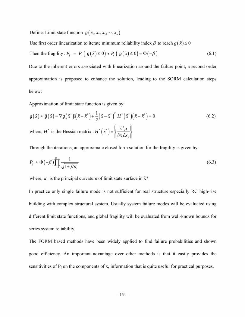
-- 164 --
( )
( )1 2 3Define: Limit state function , , , ,
Use first order linearization to iterate minimum reliability index to reach 0
ng x x x x
g xβ ≤
L
%
( )( ) ( )( ) ( ) r r Then the fragility : 0 0fP P g x P g x β= ≤ ≈ ≤ = Φ −% % (6.1)
Due to the inherent errors associated with linearization around the failure point, a second order
approximation is proposed to enhance the solution, leading to the SORM calculation steps
below:
Approximation of limit state function is given by:
( ) ( ) ( ) ( ) ( ) ( )( )* * * * * *1 02
Tg x g x g x x x x x H x x x≈ = ∇ − + − − =(
% % % % % % % % % % (6.2)
( )2
* * *where, is the Hessian matrix :i j
gH H xx x
⎧ ⎫∂⎪ ⎪= ⎨ ⎬∂ ∂⎪ ⎪⎩ ⎭%
Through the iterations, an approximate closed form solution for the fragility is given by:
( )1
1
11
n
fi i
P ββκ
−
=
≈ Φ −+
∏ (6.3)
where, is the principal curvature of limit state surface in x*iκ %
In practice only single failure mode is not sufficient for real structure especially RC high-rise
building with complex structural system. Usually system failure modes will be evaluated using
different limit state functions, and global fragility will be evaluated from well-known bounds for
series system reliability.
The FORM based methods have been widely applied to find failure probabilities and shown
good efficiency. An important advantage over other methods is that it easily provides the
sensitivities of Pf on the components of x, information that is quite useful for practical purposes.
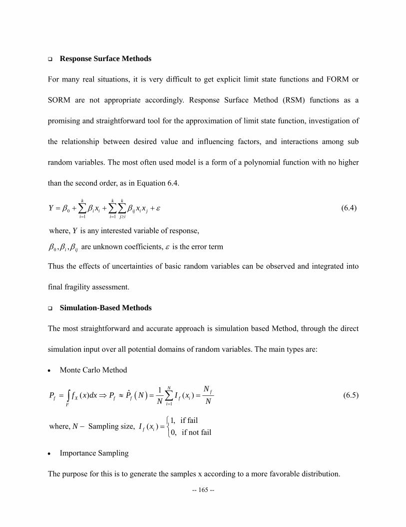
-- 165 --
Response Surface Methods
For many real situations, it is very difficult to get explicit limit state functions and FORM or
SORM are not appropriate accordingly. Response Surface Method (RSM) functions as a
promising and straightforward tool for the approximation of limit state function, investigation of
the relationship between desired value and influencing factors, and interactions among sub
random variables. The most often used model is a form of a polynomial function with no higher
than the second order, as in Equation 6.4.
01 1
k k k
i i ij i ji i j i
Y x x xβ β β ε= = ≥
= + + +∑ ∑∑ (6.4)
0
where, is any interested variable of response,
, , are unknown coefficients, is the error termi ij
Y
β β β ε
Thus the effects of uncertainties of basic random variables can be observed and integrated into
final fragility assessment.
Simulation-Based Methods
The most straightforward and accurate approach is simulation based Method, through the direct
simulation input over all potential domains of random variables. The main types are:
• Monte Carlo Method
( )1
1ˆ( ) ( )N
ff X f f f i
iF
NP f x dx P P N I x
N N=
= ⇒ ≈ = =∑∫ (6.5)
1, if failwhere, Sampling size, ( )
0, if not failf iN I x⎧
− = ⎨⎩
• Importance Sampling
The purpose for this is to generate the samples x according to a more favorable distribution.
-- 166 --
( )1
( )1ˆ ( )( )
Nx i
f f f ii i
f xP P N I x
N h x=
≈ = ∑ (6.6)
where, ( ) an optimal sampling density.ih x −
• Directional Simulation
It is a more enhanced simulation technique, for which preliminary transformation to standard
normal is required (Pinto et al. (2004)). Random variables y can be expressed in spherical
coordinates, as following:
Define: , , is unit vector of direction cosines of y r r y yθ θ= =%% %
( ) ( ) ( )f rF
P y dy f r dr f dθφ θ θ θΩ Ω Ω
⎡ ⎤= = ⎢ ⎥
⎣ ⎦∫ ∫ ∫ ∫% % (6.7)
( )( )2 20
1
1ˆ 1N
f f n ii
P P x rN
θ=
⎡ ⎤≈ = −⎣ ⎦∑ (6.8)
6.2.2 Proposed Framework
The fragility curves for the reference structure – Tower03 in Dubai will be developed using the
analytical procedures presented in Figure 6.1. Some basic features, including structural lumped
modeling, uncertainty modeling and limit state definition, have already been introduced and
accomplished earlier in previous sections. Therefore the dynamic response history analysis
(DRHA) for the evaluation of seismic demand is the main focus of the discussion below..
-- 167 --
Dynamic analyses to get seismic demand
Obtain fragility curves
RC material property uncertainties
Post-process to obtain desired values
Time history analysis using lumped model
Define limit statesMulti-resolution distributed FEM analysis
Lumped model construction
Damage measure selection
Uncertainty modeling
Direct assessment using numerical simulations
Reference RC high-rise building selection
Original frame model in ZEUS-NL
Detailed FEA of wall in VecTor2
Two-stage lumped modeling with GA
Ground motion records selection
Intensity measure selection and scaling
Figure 6.1 Proposed Analytical Fragility Assessment Framework
6.3 Numerical Simulation to Assess Fragility Relationships
6.3.1 Selection and Scaling of Intensity Measures
There are several intensity measures used by researchers to derive fragilities. The most common
ones are: peak ground acceleration (PGA) (Mosalem et al. (1997)), spectral acceleration (SA) at
some periods (Singhal and Kiremidjian (1997)), and spectral displacement (SD) at selected
periods (Rossetto and Elnashai (2003)). The choice of ground motion parameter determines the
distribution of the statistics along the horizontal axis of the fragility plot. It is expected that an
increase in the damage potential of an earthquake will coincide with an increase in the
-- 168 --
probability of building damage. A better fragility curve fit can therefore be achieved through the
choice of a ground motion parameter that correctly represents the seismic demand in terms of the
earthquake damage potential.
Selection of Intensity Measures
Elnashai et al. (2005) conducted systematic research on the selection, evaluation, and scaling of
intensity measures for ground motions. Their work assessed available techniques for scaling
strong motions and insuring a consistent level of seismic demand for a selected set of records. A
number of approaches for scaling are recommended for application to the selected records.
The PGA scaling in dynamic analyses relates the seismic forces directly to the excitation
acceleration values. It has advantages in that it is simple to apply and agrees with the methods by
which design codes normally define seismic loads. PGA has the greatest influence on structural
seismic response at high frequencies (periods less than 0.5 seconds); low-frequency structures
(periods greater than 0.5 seconds) are more sensitive to peak ground velocity (PGV) and peak
ground displacement (PGD), especially structures with very long fundamental periods (i.e.
greater than 3.0 seconds).
Another method is to use scale-based spectral parameters such as spectral acceleration, velocity,
and displacement. It may be more straightforward to select intensity according to specific periods
for certain structures. These parameters can be related to some important features within
inelasticity, such as the ductility demand imposed on structural systems when the effects of
varying yield strengths must be considered.
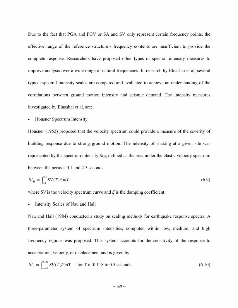
-- 169 --
Due to the fact that PGA and PGV or SA and SV only represent certain frequency points, the
effective range of the reference structure’s frequency contents are insufficient to provide the
complete response. Researchers have proposed other types of spectral intensity measures to
improve analysis over a wide range of natural frequencies. In research by Elnashai et al, several
typical spectral intensity scales are compared and evaluated to achieve an understanding of the
correlations between ground motion intensity and seismic demand. The intensity measures
investigated by Elnashai et al. are:
• Housner Spectrum Intensity
Housner (1952) proposed that the velocity spectrum could provide a measure of the severity of
building response due to strong ground motion. The intensity of shaking at a given site was
represented by the spectrum intensity SIH, defined as the area under the elastic velocity spectrum
between the periods 0.1 and 2.5 seconds:
2.5
0.1( , )HSI SV T dTξ= ∫ (6.9)
where SV is the velocity spectrum curve and ξ is the damping coefficient.
• Intensity Scales of Nau and Hall
Nau and Hall (1984) conducted a study on scaling methods for earthquake response spectra. A
three-parameter system of spectrum intensities, computed within low, medium, and high
frequency regions was proposed. This system accounts for the sensitivity of the response to
acceleration, velocity, or displacement and is given by:
0.185
0.028( , ) for T of 0.118 to 0.5 secondsaSI SV T dTξ= ∫ (6.10)
-- 170 --
2.000
0.285( , ) for T of 0.5 to 5.0 secondsvSI SV T dTξ= ∫ (6.11)
12.500
4.167( , ) for T of 5.0 to 14.085 secondsdSI SV T dTξ= ∫ (6.12)
where: SIa is the spectrum intensity in the acceleration region, SIv is the spectrum intensity in the
velocity region, and SId is the spectrum intensity in the displacement region.
• Matsumura Spectrum Intensities
Matsumura (1992) conducted a parametric study of the strong motion intensity measures and
their correlation with structural damage. SIM is referred to as the Matsumura spectrum intensity
and is defined as the mean spectral velocity between Ty and 2Ty, where Ty is the period
corresponding to yield of a single-degree-of-freedom structure (SDOF) with a critical damping
ratio ξ of 0.05. The adopted period interval [Ty, 2Ty] is based on the assumption that the response
of the structure is associated with the resonance linked to excitation frequencies around the
natural frequency of the structure.
A recent study (Martinez-Rueda (1997)) conducted an analytical examination of inelastic
performance for a large number of earthquake records in order to identify the scaling procedure
that optimizes the correlation between spectrum intensity and seismic demand represented by
displacement ductility demand. Through a parametric study of the nonlinear behavior of a SDOF
system under earthquake excitation, its correlation with various spectrum intensity scales
including SIH and SIM, as well as a third intensity scale SIyh suggested by Martinez-Rueda (1997),
significant insight was achieved. The highlights of this study are summarized below.
• Average Spectrum Intensities
To remove the different integral range influences, the spectrum intensity scales were represented
-- 171 --
as average spectrum velocities for ξ=0.05 such that:
Housner average spectrum intensity:
2.5
0.1
1 ( ,0.05)2.4HSI SV T dT= ∫ (6.13)
Matsumura average spectrum intensity:
21 ( ,0.05)y
y
T
M Ty
SI SV T dTT
= ∫ (6.14)
Martinez-Rueda (1997) suggested changing the second integration limit of Matsumura to Th,
which represents the new vibration period of the structure in the hardening range after yielding.
This was based on the assumption that the ground motion frequencies contributing to the failure
of the structure are contained within the period interval of Ty to Th. Using these integration limits,
a new average spectrum intensity is defined as:
1 ( ,0.05)h
y
T
yh Th y
SI SV T dTT T
=− ∫ (6.15)
Following a statistical evaluation of the correlation between ductility demand and considered
spectrum intensity scale using 100 accelerograms, final suggestions were made by
Martinez-Rueda (1997) for the choice of spectrum intensity scales:
(1) Long-period structures (Ty > 1.6): MSI
(2) Medium-period structures (0.6 < Ty < 1.6): HSI
(3) Short-period structures (Ty < 0.6): MSI or PGA
Using the recommended scales resulted in correlation coefficients well above 85% in most cases.
If a problem calls for the use of single spectrum intensity for simplicity, using MSI is
recommended for this purpose, provided that the period of the structure can be estimated in
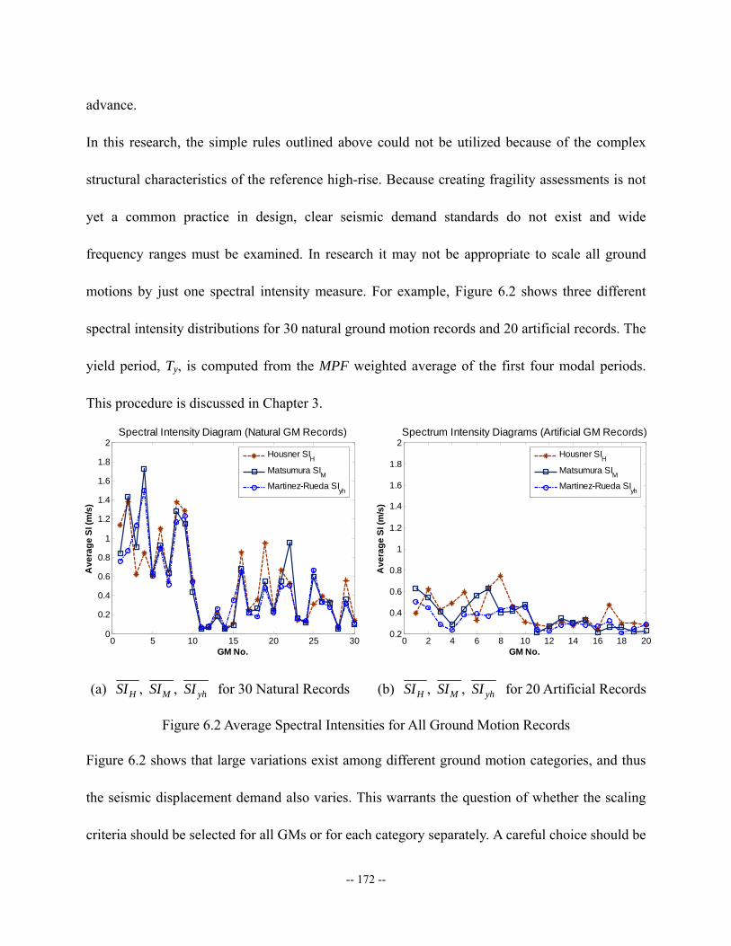
-- 172 --
advance.
In this research, the simple rules outlined above could not be utilized because of the complex
structural characteristics of the reference high-rise. Because creating fragility assessments is not
yet a common practice in design, clear seismic demand standards do not exist and wide
frequency ranges must be examined. In research it may not be appropriate to scale all ground
motions by just one spectral intensity measure. For example, Figure 6.2 shows three different
spectral intensity distributions for 30 natural ground motion records and 20 artificial records. The
yield period, Ty, is computed from the MPF weighted average of the first four modal periods.
This procedure is discussed in Chapter 3.
0 5 10 15 20 25 300
0.2
0.4
0.6
0.8
1
1.2
1.4
1.6
1.8
2
GM No.
Ave
rage
SI (
m/s
)
Spectral Intensity Diagram (Natural GM Records)
Housner SIHMatsumura SIMMartinez-Rueda SIyh
0 2 4 6 8 10 12 14 16 18 200.2
0.4
0.6
0.8
1
1.2
1.4
1.6
1.8
2
GM No.
Ave
rage
SI (
m/s
)
Spectrum Intensity Diagrams (Artificial GM Records)
Housner SIHMatsumura SIMMartinez-Rueda SIyh
(a) , , H M yhSI SI SI for 30 Natural Records (b) , , H M yhSI SI SI for 20 Artificial Records
Figure 6.2 Average Spectral Intensities for All Ground Motion Records
Figure 6.2 shows that large variations exist among different ground motion categories, and thus
the seismic displacement demand also varies. This warrants the question of whether the scaling
criteria should be selected for all GMs or for each category separately. A careful choice should be
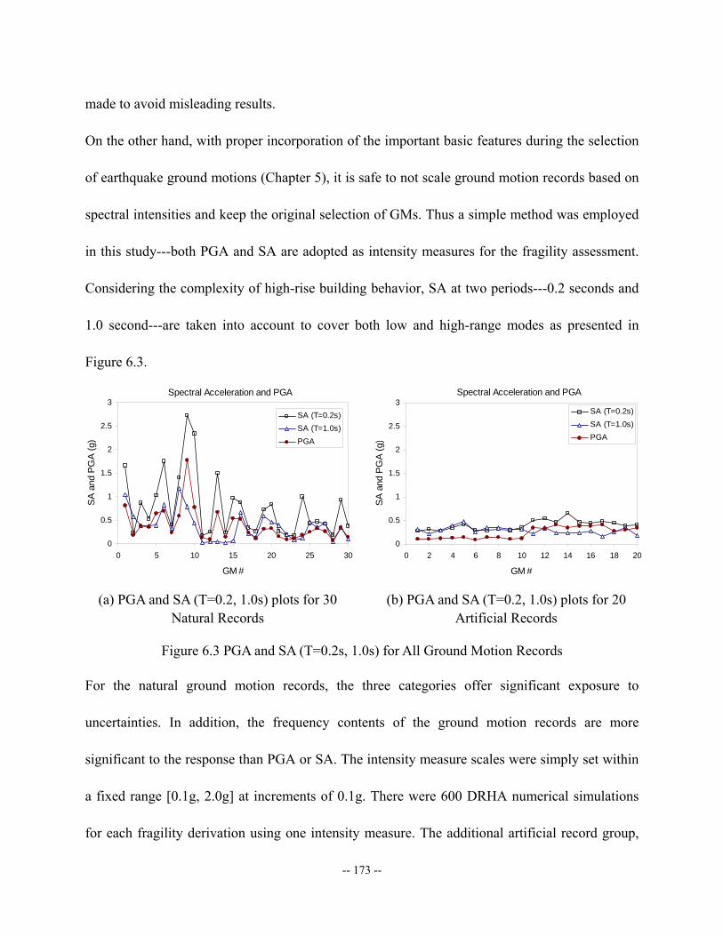
-- 173 --
made to avoid misleading results.
On the other hand, with proper incorporation of the important basic features during the selection
of earthquake ground motions (Chapter 5), it is safe to not scale ground motion records based on
spectral intensities and keep the original selection of GMs. Thus a simple method was employed
in this study---both PGA and SA are adopted as intensity measures for the fragility assessment.
Considering the complexity of high-rise building behavior, SA at two periods---0.2 seconds and
1.0 second---are taken into account to cover both low and high-range modes as presented in
Figure 6.3.
Spectral Acceleration and PGA
0
0.5
1
1.5
2
2.5
3
0 5 10 15 20 25 30
GM #
SA
and
PGA
(g)
SA (T=0.2s)SA (T=1.0s)PGA
Spectral Acceleration and PGA
0
0.5
1
1.5
2
2.5
3
0 2 4 6 8 10 12 14 16 18 20
GM #
SA a
nd P
GA
(g)
SA (T=0.2s)SA (T=1.0s)PGA
(a) PGA and SA (T=0.2, 1.0s) plots for 30 Natural Records
(b) PGA and SA (T=0.2, 1.0s) plots for 20 Artificial Records
Figure 6.3 PGA and SA (T=0.2s, 1.0s) for All Ground Motion Records
For the natural ground motion records, the three categories offer significant exposure to
uncertainties. In addition, the frequency contents of the ground motion records are more
significant to the response than PGA or SA. The intensity measure scales were simply set within
a fixed range [0.1g, 2.0g] at increments of 0.1g. There were 600 DRHA numerical simulations
for each fragility derivation using one intensity measure. The additional artificial record group,
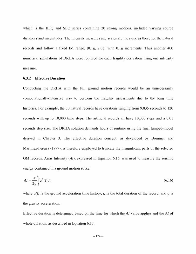
-- 174 --
which is the BEQ and SEQ series containing 20 strong motions, included varying source
distances and magnitudes. The intensity measures and scales are the same as those for the natural
records and follow a fixed IM range, [0.1g, 2.0g] with 0.1g increments. Thus another 400
numerical simulations of DRHA were required for each fragility derivation using one intensity
measure.
6.3.2 Effective Duration
Conducting the DRHA with the full ground motion records would be an unnecessarily
computationally-intensive way to perform the fragility assessments due to the long time
histories. For example, the 30 natural records have durations ranging from 9.835 seconds to 120
seconds with up to 18,000 time steps. The artificial records all have 10,000 steps and a 0.01
seconds step size. The DRHA solution demands hours of runtime using the final lumped-model
derived in Chapter 3. The effective duration concept, as developed by Bommer and
Martinez-Pereira (1999), is therefore employed to truncate the insignificant parts of the selected
GM records. Arias Intensity (AI), expressed in Equation 6.16, was used to measure the seismic
energy contained in a ground motion strike.
2
0
( )2
rt
AI a t dtgπ
= ∫ (6.16)
where a(t) is the ground acceleration time history, tr is the total duration of the record, and g is
the gravity acceleration.
Effective duration is determined based on the time for which the AI value applies and the AI of
whole duration, as described in Equation 6.17.
-- 175 --
f oDE t t= − (6.17)
where, -- the effective duration
, -- the ending and starting time of f o
DE
t t DE
Based on the significant duration concept, Bommer and Martinez-Pereira (1999) suggested that
the start and end of the strong motion be identified by the absolute criteria:
0.01 / ; 0.125 /o f total fAI m s AI AI AI m s= Δ = − = (6.18)
where, , represent values up to and the remaining of the period after o f o fAI AI AI t t .
In cases where some records have very low AItotal values, using only absolute criteria will be
insufficient and misleading, and relative ratio limits are employed to provide additional restraints
and avoid the underestimation of structural seismic responses. The effective duration also needs
to satisfy:
0.5% ; 95.5% o total f totalAI AI AI AI≤ ≥ (6.19)
Through the application of the criteria above, effective durations were derived for all selected
accelerograms, and one example is shown in Figure 6.4.
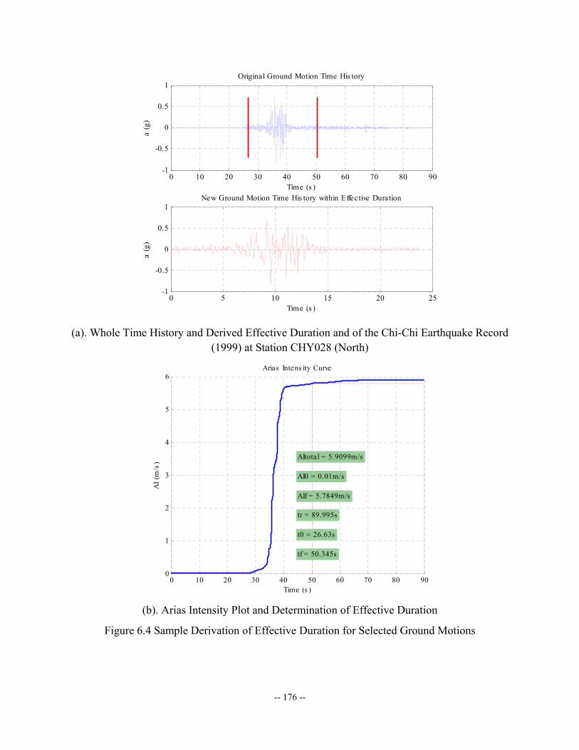
-- 176 --
0 10 20 30 40 50 60 70 80 90-1
-0.5
0
0.5
1
Time (s )
a (g
)
Original Ground Motion Time His tory
0 5 10 15 20 25-1
-0.5
0
0.5
1
Time (s )
a (g
)
New Ground Motion Time His tory within Effective Duration
(a). Whole Time History and Derived Effective Duration and of the Chi-Chi Earthquake Record (1999) at Station CHY028 (North)
0 10 20 30 40 50 60 70 80 900
1
2
3
4
5
6Arias Intens ity Curve
Time (s )
AI (
m/s
)
AItotal = 5.9099m/s
AI0 = 0.01m/s
AIf = 5.7849m/s
tr = 89.995s
t0 = 26.63s
tf = 50.345s
(b). Arias Intensity Plot and Determination of Effective Duration
Figure 6.4 Sample Derivation of Effective Duration for Selected Ground Motions
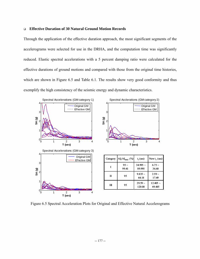
-- 177 --
Effective Duration of 30 Natural Ground Motion Records
Through the application of the effective duration approach, the most significant segments of the
accelerograms were selected for use in the DRHA, and the computation time was significantly
reduced. Elastic spectral accelerations with a 5 percent damping ratio were calculated for the
effective durations of ground motions and compared with those from the original time histories,
which are shown in Figure 6.5 and Table 6.1. The results show very good conformity and thus
exemplify the high consistency of the seismic energy and dynamic characteristics.
0 1 2 3 40
1
2
3
4Spectral Accelerations (GM category 1)
T (sec)
SA (g
)
0 1 2 3 40
1
2
3
4Spectral Acclerations (GM category 2)
T (sec)
SA (g
)
0 1 2 3 40
1
2
3
4Spectral Accelerations (GM category 3)
T (sec)
SA (g
)
Original GMEffective GM
Original GMEffective GM
Original GMEffective GM Category AIf/AItotal (%) tr (sec) New tr (sec)
I95 ~
99.4134.995 ~ 89.995
6.75 ~ 36.60
II 959.835 ~ 44.18
2.59 ~ 17.49
III 9529.59 ~ 120.00
12.405 ~ 49.485
Category AIf/AItotal (%) tr (sec) New tr (sec)
I95 ~
99.4134.995 ~ 89.995
6.75 ~ 36.60
II 959.835 ~ 44.18
2.59 ~ 17.49
III 9529.59 ~ 120.00
12.405 ~ 49.485
Figure 6.5 Spectral Acceleration Plots for Original and Effective Natural Accelerograms
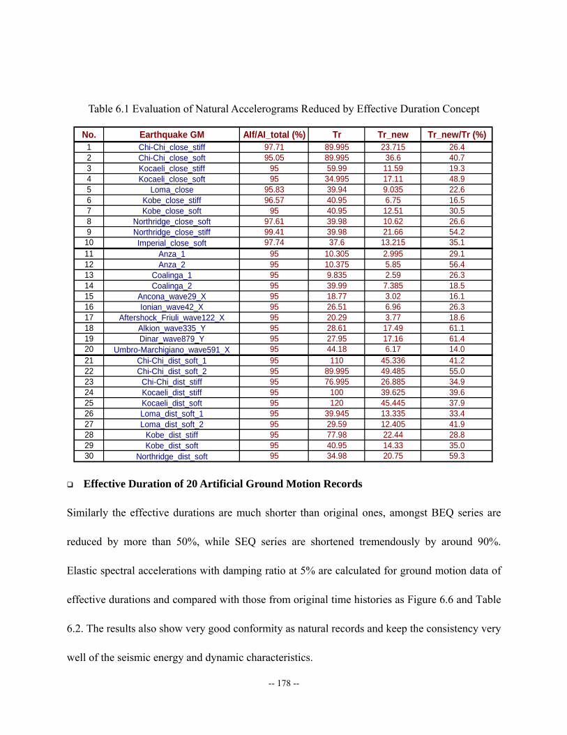
-- 178 --
Table 6.1 Evaluation of Natural Accelerograms Reduced by Effective Duration Concept
No. Earthquake GM AIf/AI_total (%) Tr Tr_new Tr_new/Tr (%)1 Chi-Chi_close_stiff 97.71 89.995 23.715 26.42 Chi-Chi_close_soft 95.05 89.995 36.6 40.73 Kocaeli_close_stiff 95 59.99 11.59 19.34 Kocaeli_close_soft 95 34.995 17.11 48.95 Loma_close 95.83 39.94 9.035 22.66 Kobe_close_stiff 96.57 40.95 6.75 16.57 Kobe_close_soft 95 40.95 12.51 30.58 Northridge_close_soft 97.61 39.98 10.62 26.69 Northridge_close_stiff 99.41 39.98 21.66 54.2
10 Imperial_close_soft 97.74 37.6 13.215 35.111 Anza_1 95 10.305 2.995 29.112 Anza_2 95 10.375 5.85 56.413 Coalinga_1 95 9.835 2.59 26.314 Coalinga_2 95 39.99 7.385 18.515 Ancona_wave29_X 95 18.77 3.02 16.116 Ionian_wave42_X 95 26.51 6.96 26.317 Aftershock_Friuli_wave122_X 95 20.29 3.77 18.618 Alkion_wave335_Y 95 28.61 17.49 61.119 Dinar_wave879_Y 95 27.95 17.16 61.420 Umbro-Marchigiano_wave591_X 95 44.18 6.17 14.021 Chi-Chi_dist_soft_1 95 110 45.336 41.222 Chi-Chi_dist_soft_2 95 89.995 49.485 55.023 Chi-Chi_dist_stiff 95 76.995 26.885 34.924 Kocaeli_dist_stiff 95 100 39.625 39.625 Kocaeli_dist_soft 95 120 45.445 37.926 Loma_dist_soft_1 95 39.945 13.335 33.427 Loma_dist_soft_2 95 29.59 12.405 41.928 Kobe_dist_stiff 95 77.98 22.44 28.829 Kobe_dist_soft 95 40.95 14.33 35.030 Northridge_dist_soft 95 34.98 20.75 59.3
Effective Duration of 20 Artificial Ground Motion Records
Similarly the effective durations are much shorter than original ones, amongst BEQ series are
reduced by more than 50%, while SEQ series are shortened tremendously by around 90%.
Elastic spectral accelerations with damping ratio at 5% are calculated for ground motion data of
effective durations and compared with those from original time histories as Figure 6.6 and Table
6.2. The results also show very good conformity as natural records and keep the consistency very
well of the seismic energy and dynamic characteristics.
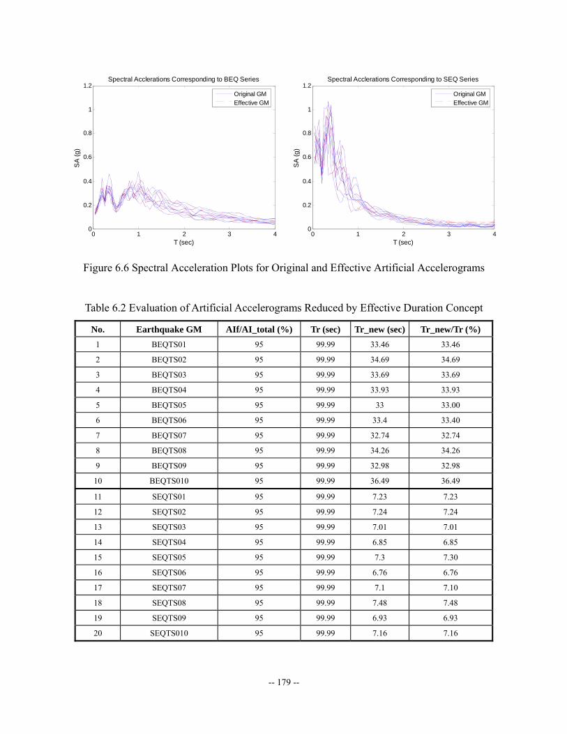
-- 179 --
0 1 2 3 40
0.2
0.4
0.6
0.8
1
1.2Spectral Acclerations Corresponding to BEQ Series
T (sec)
SA
(g)
Original GMEffective GM
0 1 2 3 4
0
0.2
0.4
0.6
0.8
1
1.2Spectral Acclerations Corresponding to SEQ Series
T (sec)
SA
(g)
Original GMEffective GM
Figure 6.6 Spectral Acceleration Plots for Original and Effective Artificial Accelerograms
Table 6.2 Evaluation of Artificial Accelerograms Reduced by Effective Duration Concept
No. Earthquake GM AIf/AI_total (%) Tr (sec) Tr_new (sec) Tr_new/Tr (%) 1 BEQTS01 95 99.99 33.46 33.46
2 BEQTS02 95 99.99 34.69 34.69
3 BEQTS03 95 99.99 33.69 33.69
4 BEQTS04 95 99.99 33.93 33.93
5 BEQTS05 95 99.99 33 33.00
6 BEQTS06 95 99.99 33.4 33.40
7 BEQTS07 95 99.99 32.74 32.74
8 BEQTS08 95 99.99 34.26 34.26
9 BEQTS09 95 99.99 32.98 32.98
10 BEQTS010 95 99.99 36.49 36.49
11 SEQTS01 95 99.99 7.23 7.23
12 SEQTS02 95 99.99 7.24 7.24
13 SEQTS03 95 99.99 7.01 7.01
14 SEQTS04 95 99.99 6.85 6.85
15 SEQTS05 95 99.99 7.3 7.30
16 SEQTS06 95 99.99 6.76 6.76
17 SEQTS07 95 99.99 7.1 7.10
18 SEQTS08 95 99.99 7.48 7.48
19 SEQTS09 95 99.99 6.93 6.93
20 SEQTS010 95 99.99 7.16 7.16
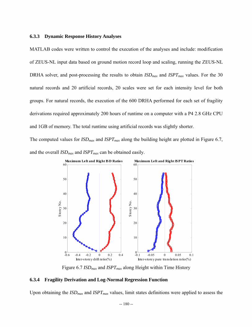
-- 180 --
6.3.3 Dynamic Response History Analyses
MATLAB codes were written to control the execution of the analyses and include: modification
of ZEUS-NL input data based on ground motion record loop and scaling, running the ZEUS-NL
DRHA solver, and post-processing the results to obtain ISDmax and ISPTmax values. For the 30
natural records and 20 artificial records, 20 scales were set for each intensity level for both
groups. For natural records, the execution of the 600 DRHA performed for each set of fragility
derivations required approximately 200 hours of runtime on a computer with a P4 2.8 GHz CPU
and 1GB of memory. The total runtime using artificial records was slightly shorter.
The computed values for ISDmax and ISPTmax along the building height are plotted in Figure 6.7,
and the overall ISDmax and ISPTmax can be obtained easily.
-0.6 -0.4 -0.2 0 0.2 0.40
10
20
30
40
50
60
Inte r-s torey drift ra tio(%)
Sto
rey
No.
Maximum Left and Right IS D Ratio s
-0.1 -0.05 0 0.05 0.10
10
20
30
40
50
60
Inte r-s torey pure trans la tion ra tio(%)
Sto
rey
No.
Maximum Left and Rig ht IS PT Ratios
Figure 6.7 ISDmax and ISPTmax along Height within Time History
6.3.4 Fragility Derivation and Log-Normal Regression Function
Upon obtaining the ISDmax and ISPTmax values, limit states definitions were applied to assess the
-- 181 --
performance levels of the building subjected to a particular ground excitation. If the computed
values were larger than a limit state level for either ISDmax or ISPTmax, the event that exceeded
the LS was counted within the sample containing all GM scales. The direct sampling probability
for each type of intensity measure over the 30 selected natural and 20 artificial GMs on all 20
scales were thereby assessed.
It was not possible to complete the full DRHA for all GM records at all scales due to
non-convergence in some analyses. ZEUS-NL automatically reduces the step size down to 1/100
of the original time step if the convergence is not achieved. If the solution does not converge at
the reduced time step, then subsequent results are not trustworthy, and the DRHA is terminated
for that run. This failure to converge can be a result of material inelasticity or geometric
nonlinearity at some local elements, and it does not necessarily indicate the structure is near
collapse. When an analysis run failed due to lack of convergence, it was necessary to determine
whether the analysis was predicting collapse, or the lack of convergence was caused by another
issue for which the analysis results should be dismissed. For a structure to be judged near
collapse, one of the following conditions had to be satisfied:
• ISDmax or ISPTmax at current GM scale exceeded limit state 3 (LS3) before divergence;
• ISDmax or ISPTmax at previous GM scale exceeded LS3;
• ISDmax or ISPTmax at previous GM scale were close to the LS3 (within 90%), and the
current values were larger than values from the previous time step.
For situations not listed above, it was necessary to assess the performance level based on a
comparison between the calculated maximum values and defined limit state values. The
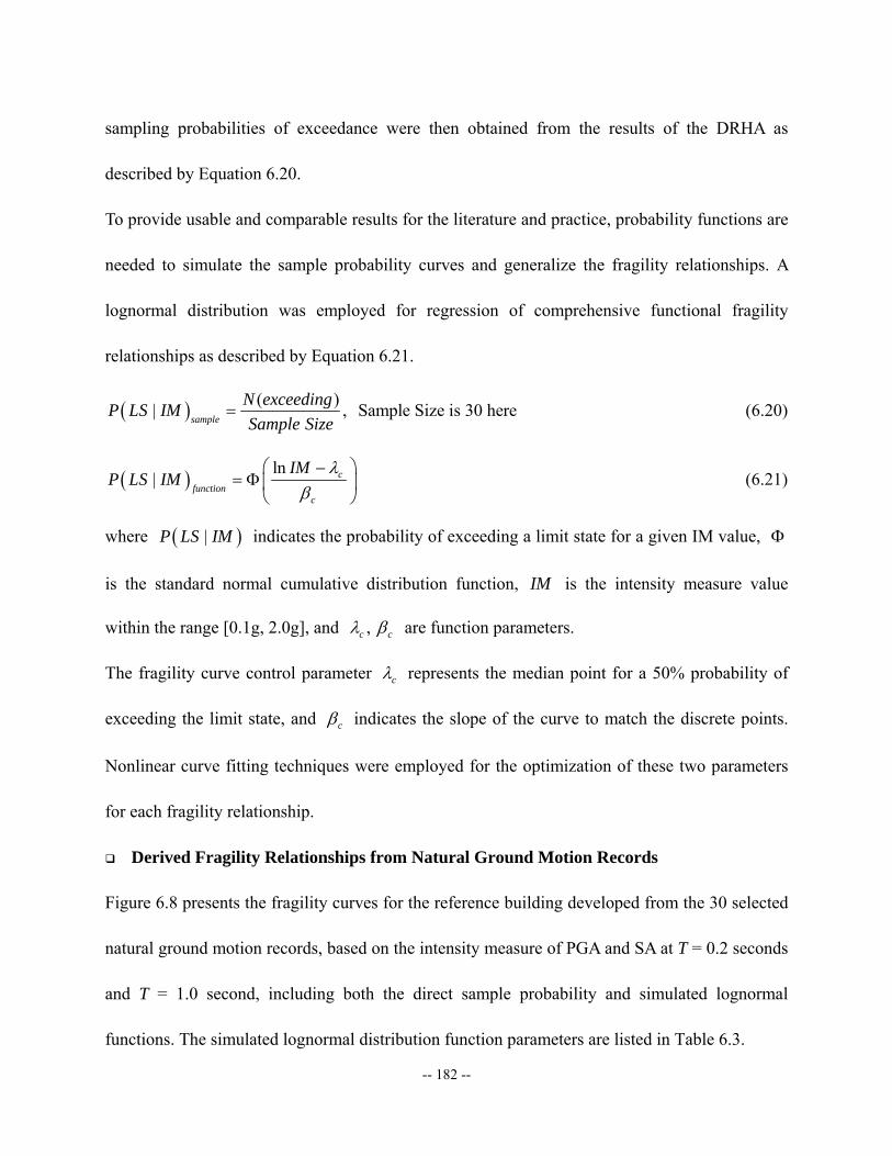
-- 182 --
sampling probabilities of exceedance were then obtained from the results of the DRHA as
described by Equation 6.20.
To provide usable and comparable results for the literature and practice, probability functions are
needed to simulate the sample probability curves and generalize the fragility relationships. A
lognormal distribution was employed for regression of comprehensive functional fragility
relationships as described by Equation 6.21.
( ) ( )| , Sample Size is 30 here sample
N exceedingP LS IMSample Size
= (6.20)
( ) ln| c
functionc
IMP LS IM
λβ
⎛ ⎞−= Φ⎜ ⎟
⎝ ⎠ (6.21)
where ( )|P LS IM indicates the probability of exceeding a limit state for a given IM value, Φ
is the standard normal cumulative distribution function, IM is the intensity measure value
within the range [0.1g, 2.0g], and , c cλ β are function parameters.
The fragility curve control parameter cλ represents the median point for a 50% probability of
exceeding the limit state, and cβ indicates the slope of the curve to match the discrete points.
Nonlinear curve fitting techniques were employed for the optimization of these two parameters
for each fragility relationship.
Derived Fragility Relationships from Natural Ground Motion Records
Figure 6.8 presents the fragility curves for the reference building developed from the 30 selected
natural ground motion records, based on the intensity measure of PGA and SA at T = 0.2 seconds
and T = 1.0 second, including both the direct sample probability and simulated lognormal
functions. The simulated lognormal distribution function parameters are listed in Table 6.3.
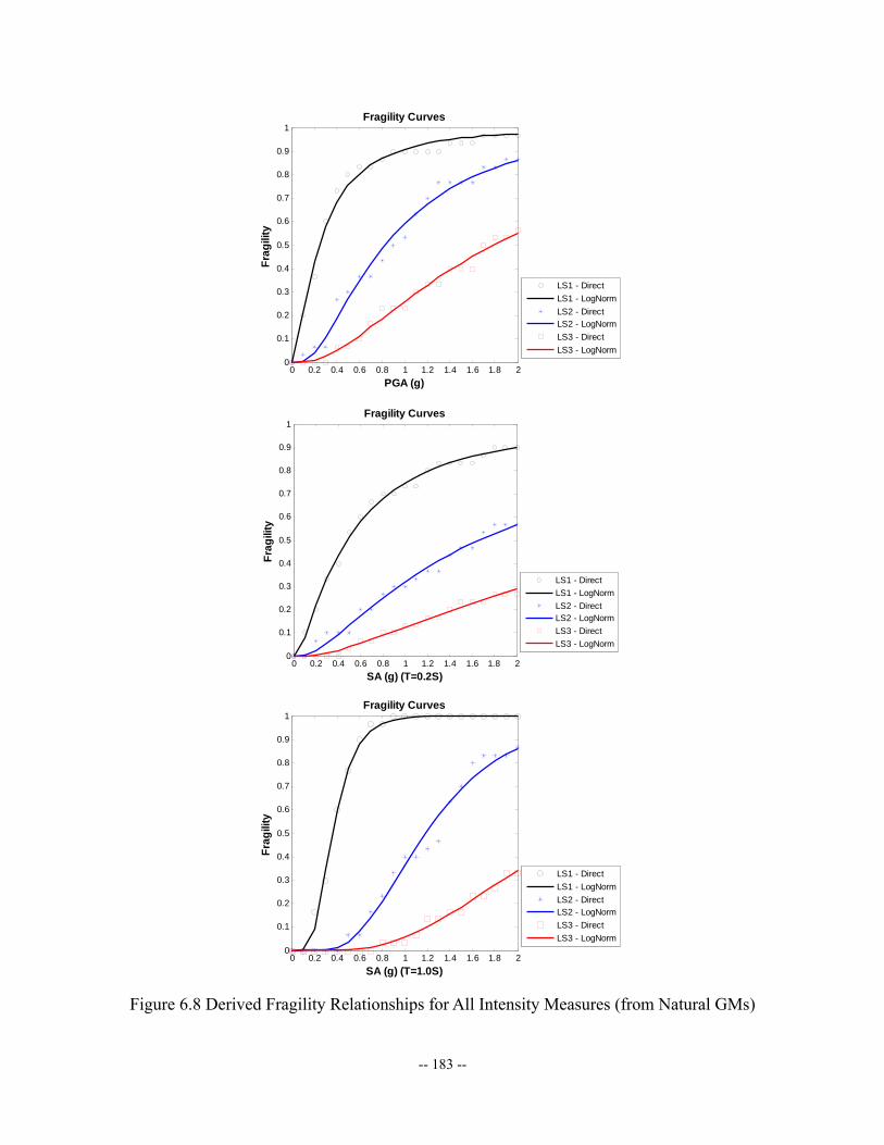
-- 183 --
0 0.2 0.4 0.6 0.8 1 1.2 1.4 1.6 1.8 20
0.1
0.2
0.3
0.4
0.5
0.6
0.7
0.8
0.9
1
PGA (g)
Frag
ility
Fragility Curves
LS1 - DirectLS1 - LogNormLS2 - DirectLS2 - LogNormLS3 - DirectLS3 - LogNorm
0 0.2 0.4 0.6 0.8 1 1.2 1.4 1.6 1.8 20
0.1
0.2
0.3
0.4
0.5
0.6
0.7
0.8
0.9
1
SA (g) (T=0.2S)
Frag
ility
Fragility Curves
LS1 - DirectLS1 - LogNormLS2 - DirectLS2 - LogNormLS3 - DirectLS3 - LogNorm
0 0.2 0.4 0.6 0.8 1 1.2 1.4 1.6 1.8 20
0.1
0.2
0.3
0.4
0.5
0.6
0.7
0.8
0.9
1
SA (g) (T=1.0S)
Frag
ility
Fragility Curves
LS1 - DirectLS1 - LogNormLS2 - DirectLS2 - LogNormLS3 - DirectLS3 - LogNorm
Figure 6.8 Derived Fragility Relationships for All Intensity Measures (from Natural GMs)
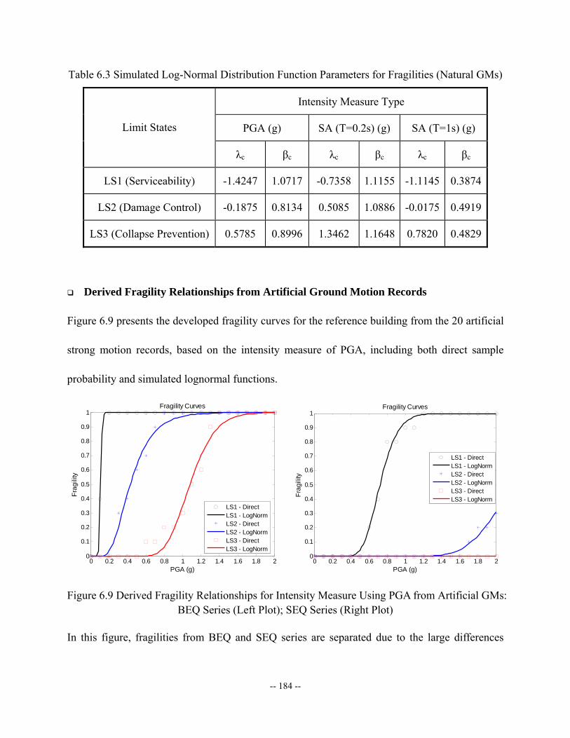
-- 184 --
Table 6.3 Simulated Log-Normal Distribution Function Parameters for Fragilities (Natural GMs)
Intensity Measure Type
PGA (g) SA (T=0.2s) (g) SA (T=1s) (g) Limit States
λc βc λc βc λc βc
LS1 (Serviceability) -1.4247 1.0717 -0.7358 1.1155 -1.1145 0.3874
LS2 (Damage Control) -0.1875 0.8134 0.5085 1.0886 -0.0175 0.4919
LS3 (Collapse Prevention) 0.5785 0.8996 1.3462 1.1648 0.7820 0.4829
Derived Fragility Relationships from Artificial Ground Motion Records
Figure 6.9 presents the developed fragility curves for the reference building from the 20 artificial
strong motion records, based on the intensity measure of PGA, including both direct sample
probability and simulated lognormal functions.
0 0.2 0.4 0.6 0.8 1 1.2 1.4 1.6 1.8 20
0.1
0.2
0.3
0.4
0.5
0.6
0.7
0.8
0.9
1
PGA (g)
Frag
ility
Fragility Curves
LS1 - DirectLS1 - LogNormLS2 - DirectLS2 - LogNormLS3 - DirectLS3 - LogNorm
0 0.2 0.4 0.6 0.8 1 1.2 1.4 1.6 1.8 2
0
0.1
0.2
0.3
0.4
0.5
0.6
0.7
0.8
0.9
1
PGA (g)
Frag
ility
Fragility Curves
LS1 - DirectLS1 - LogNormLS2 - DirectLS2 - LogNormLS3 - DirectLS3 - LogNorm
Figure 6.9 Derived Fragility Relationships for Intensity Measure Using PGA from Artificial GMs: BEQ Series (Left Plot); SEQ Series (Right Plot)
In this figure, fragilities from BEQ and SEQ series are separated due to the large differences
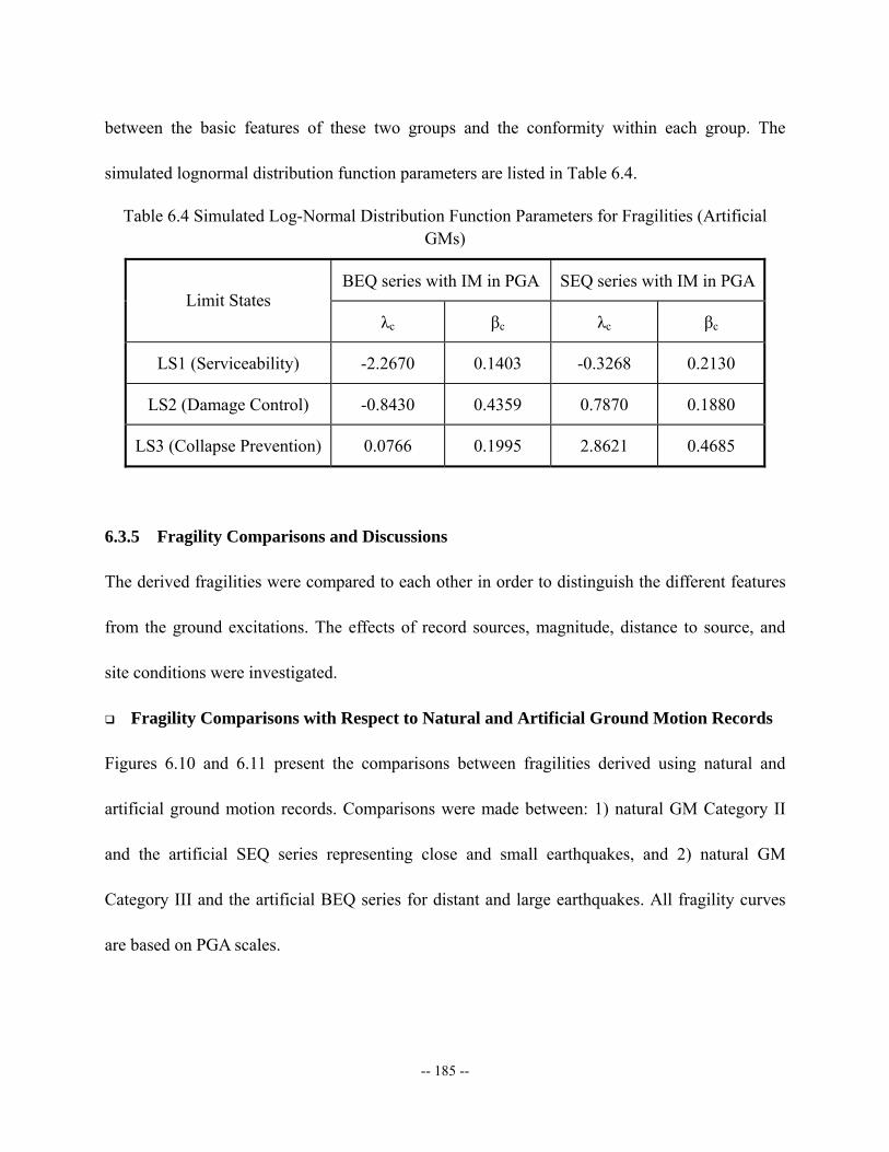
-- 185 --
between the basic features of these two groups and the conformity within each group. The
simulated lognormal distribution function parameters are listed in Table 6.4.
Table 6.4 Simulated Log-Normal Distribution Function Parameters for Fragilities (Artificial GMs)
BEQ series with IM in PGA SEQ series with IM in PGALimit States
λc βc λc βc
LS1 (Serviceability) -2.2670 0.1403 -0.3268 0.2130
LS2 (Damage Control) -0.8430 0.4359 0.7870 0.1880
LS3 (Collapse Prevention) 0.0766 0.1995 2.8621 0.4685
6.3.5 Fragility Comparisons and Discussions
The derived fragilities were compared to each other in order to distinguish the different features
from the ground excitations. The effects of record sources, magnitude, distance to source, and
site conditions were investigated.
Fragility Comparisons with Respect to Natural and Artificial Ground Motion Records
Figures 6.10 and 6.11 present the comparisons between fragilities derived using natural and
artificial ground motion records. Comparisons were made between: 1) natural GM Category II
and the artificial SEQ series representing close and small earthquakes, and 2) natural GM
Category III and the artificial BEQ series for distant and large earthquakes. All fragility curves
are based on PGA scales.
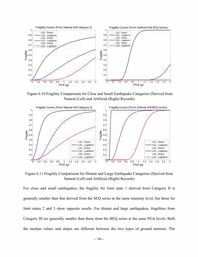
-- 186 --
0 0.2 0.4 0.6 0.8 1 1.2 1.4 1.6 1.8 20
0.1
0.2
0.3
0.4
0.5
0.6
0.7
0.8
0.9
1
PGA (g)
Frag
ility
Fragility Curves (From Natural GM category 2)
LS1 - DirectLS1 - LogNormLS2 - DirectLS2 - LogNormLS3 - DirectLS3 - LogNorm
0 0.2 0.4 0.6 0.8 1 1.2 1.4 1.6 1.8 20
0.1
0.2
0.3
0.4
0.5
0.6
0.7
0.8
0.9
1
PGA (g)
Frag
ility
Fragility Curves (From Artificial GM SEQ series)
LS1 - DirectLS1 - LogNormLS2 - DirectLS2 - LogNormLS3 - DirectLS3 - LogNorm
Figure 6.10 Fragility Comparisons for Close and Small Earthquake Categories (Derived from Natural (Left) and Artificial (Right) Records)
0 0.2 0.4 0.6 0.8 1 1.2 1.4 1.6 1.8 20
0.1
0.2
0.3
0.4
0.5
0.6
0.7
0.8
0.9
1
PGA (g)
Frag
ility
Fragility Curves (From Natural GM Category 3)
LS1 - DirectLS1 - LogNormLS2 - DirectLS2 - LogNormLS3 - DirectLS3 - LogNorm
0 0.2 0.4 0.6 0.8 1 1.2 1.4 1.6 1.8 20
0.1
0.2
0.3
0.4
0.5
0.6
0.7
0.8
0.9
1
PGA (g)
Frag
ility
Fragility Curves (From Artificial GM BEQ series)
LS1 - DirectLS1 - LogNormLS2 - DirectLS2 - LogNormLS3 - DirectLS3 - LogNorm
Figure 6.11 Fragility Comparisons for Distant and Large Earthquake Categories (Derived from Natural (Left) and Artificial (Right) Records)
For close and small earthquakes, the fragility for limit state 1 derived from Category II is
generally smaller than that derived from the SEQ series at the same intensity level, but those for
limit states 2 and 3 show opposite results. For distant and large earthquakes, fragilities from
Category III are generally smaller than those from the BEQ series at the same PGA levels. Both
the median values and slopes are different between the two types of ground motions. The
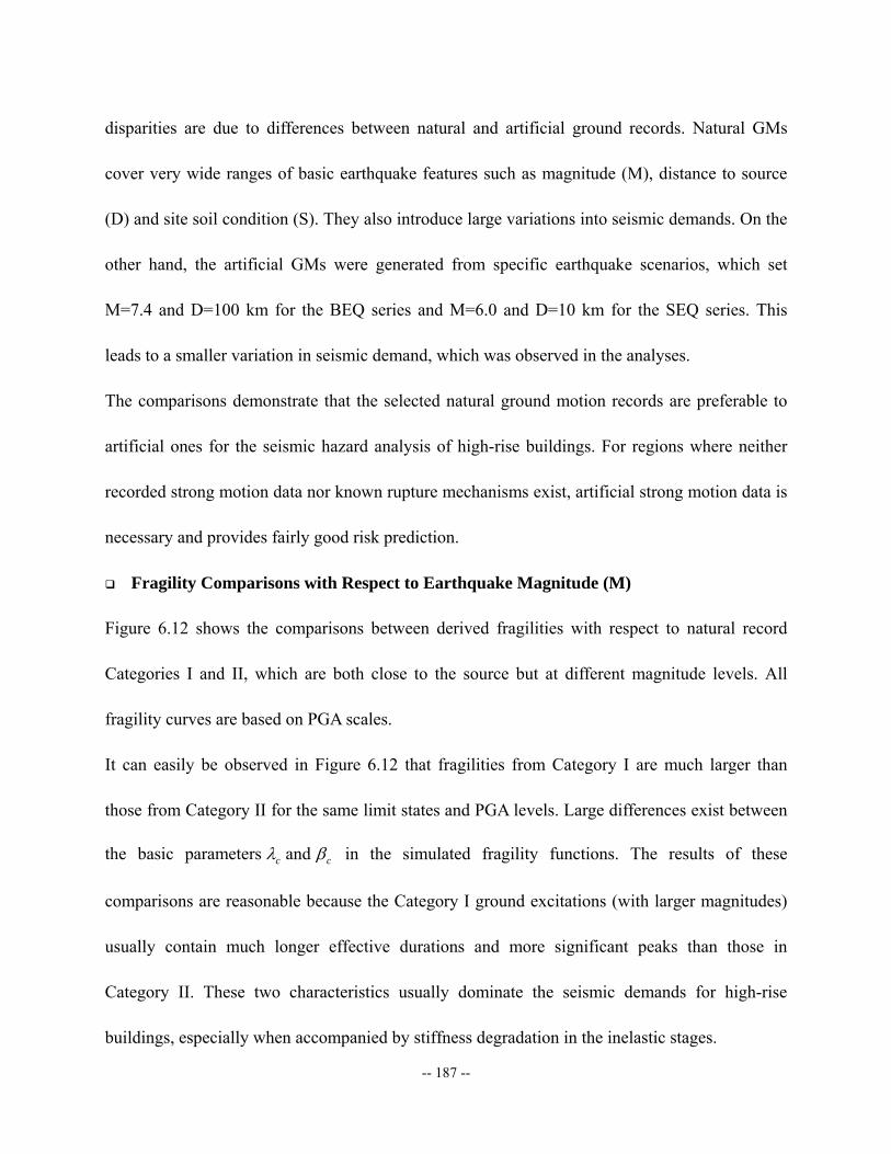
-- 187 --
disparities are due to differences between natural and artificial ground records. Natural GMs
cover very wide ranges of basic earthquake features such as magnitude (M), distance to source
(D) and site soil condition (S). They also introduce large variations into seismic demands. On the
other hand, the artificial GMs were generated from specific earthquake scenarios, which set
M=7.4 and D=100 km for the BEQ series and M=6.0 and D=10 km for the SEQ series. This
leads to a smaller variation in seismic demand, which was observed in the analyses.
The comparisons demonstrate that the selected natural ground motion records are preferable to
artificial ones for the seismic hazard analysis of high-rise buildings. For regions where neither
recorded strong motion data nor known rupture mechanisms exist, artificial strong motion data is
necessary and provides fairly good risk prediction.
Fragility Comparisons with Respect to Earthquake Magnitude (M)
Figure 6.12 shows the comparisons between derived fragilities with respect to natural record
Categories I and II, which are both close to the source but at different magnitude levels. All
fragility curves are based on PGA scales.
It can easily be observed in Figure 6.12 that fragilities from Category I are much larger than
those from Category II for the same limit states and PGA levels. Large differences exist between
the basic parameters cλ and cβ in the simulated fragility functions. The results of these
comparisons are reasonable because the Category I ground excitations (with larger magnitudes)
usually contain much longer effective durations and more significant peaks than those in
Category II. These two characteristics usually dominate the seismic demands for high-rise
buildings, especially when accompanied by stiffness degradation in the inelastic stages.
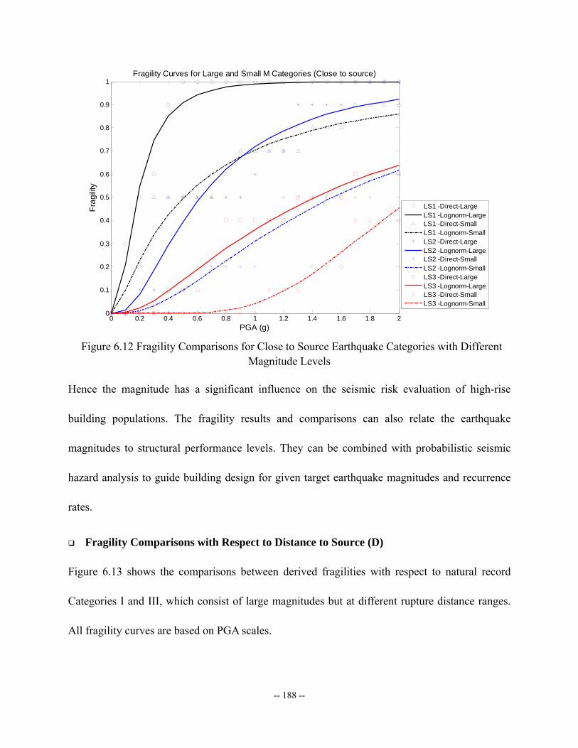
-- 188 --
0 0.2 0.4 0.6 0.8 1 1.2 1.4 1.6 1.8 20
0.1
0.2
0.3
0.4
0.5
0.6
0.7
0.8
0.9
1
PGA (g)
Frag
ility
Fragility Curves for Large and Small M Categories (Close to source)
LS1 -Direct-LargeLS1 -Lognorm-LargeLS1 -Direct-SmallLS1 -Lognorm-SmallLS2 -Direct-LargeLS2 -Lognorm-LargeLS2 -Direct-SmallLS2 -Lognorm-SmallLS3 -Direct-LargeLS3 -Lognorm-LargeLS3 -Direct-SmallLS3 -Lognorm-Small
Figure 6.12 Fragility Comparisons for Close to Source Earthquake Categories with Different
Magnitude Levels
Hence the magnitude has a significant influence on the seismic risk evaluation of high-rise
building populations. The fragility results and comparisons can also relate the earthquake
magnitudes to structural performance levels. They can be combined with probabilistic seismic
hazard analysis to guide building design for given target earthquake magnitudes and recurrence
rates.
Fragility Comparisons with Respect to Distance to Source (D)
Figure 6.13 shows the comparisons between derived fragilities with respect to natural record
Categories I and III, which consist of large magnitudes but at different rupture distance ranges.
All fragility curves are based on PGA scales.
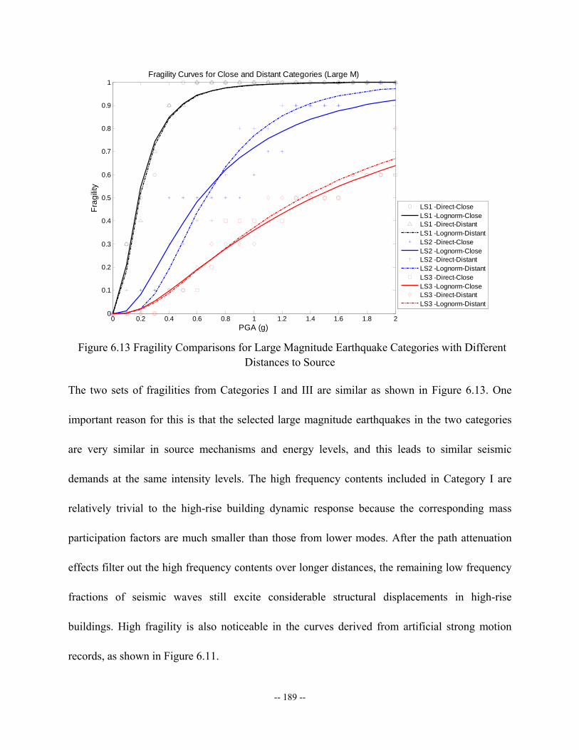
-- 189 --
0 0.2 0.4 0.6 0.8 1 1.2 1.4 1.6 1.8 20
0.1
0.2
0.3
0.4
0.5
0.6
0.7
0.8
0.9
1
PGA (g)
Frag
ility
Fragility Curves for Close and Distant Categories (Large M)
LS1 -Direct-CloseLS1 -Lognorm-CloseLS1 -Direct-DistantLS1 -Lognorm-DistantLS2 -Direct-CloseLS2 -Lognorm-CloseLS2 -Direct-DistantLS2 -Lognorm-DistantLS3 -Direct-CloseLS3 -Lognorm-CloseLS3 -Direct-DistantLS3 -Lognorm-Distant
Figure 6.13 Fragility Comparisons for Large Magnitude Earthquake Categories with Different
Distances to Source
The two sets of fragilities from Categories I and III are similar as shown in Figure 6.13. One
important reason for this is that the selected large magnitude earthquakes in the two categories
are very similar in source mechanisms and energy levels, and this leads to similar seismic
demands at the same intensity levels. The high frequency contents included in Category I are
relatively trivial to the high-rise building dynamic response because the corresponding mass
participation factors are much smaller than those from lower modes. After the path attenuation
effects filter out the high frequency contents over longer distances, the remaining low frequency
fractions of seismic waves still excite considerable structural displacements in high-rise
buildings. High fragility is also noticeable in the curves derived from artificial strong motion
records, as shown in Figure 6.11.
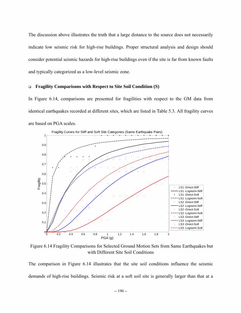
-- 190 --
The discussion above illustrates the truth that a large distance to the source does not necessarily
indicate low seismic risk for high-rise buildings. Proper structural analysis and design should
consider potential seismic hazards for high-rise buildings even if the site is far from known faults
and typically categorized as a low-level seismic zone.
Fragility Comparisons with Respect to Site Soil Condition (S)
In Figure 6.14, comparisons are presented for fragilities with respect to the GM data from
identical earthquakes recorded at different sites, which are listed in Table 5.3. All fragility curves
are based on PGA scales.
0 0.2 0.4 0.6 0.8 1 1.2 1.4 1.6 1.8 20
0.1
0.2
0.3
0.4
0.5
0.6
0.7
0.8
0.9
1
PGA (g)
Frag
ility
Fragility Curves for Stiff and Soft Site Categories (Same Earthquake Pairs)
LS1 -Direct-StiffLS1 -Lognorm-StiffLS1 -Direct-SoftLS1 -Lognorm-SoftLS2 -Direct-StiffLS2 -Lognorm-StiffLS2 -Direct-SoftLS2 -Lognorm-SoftLS3 -Direct-StiffLS3 -Lognorm-StiffLS3 -Direct-SoftLS3 -Lognorm-Soft
Figure 6.14 Fragility Comparisons for Selected Ground Motion Sets from Same Earthquakes but
with Different Site Soil Conditions
The comparison in Figure 6.14 illustrates that the site soil conditions influence the seismic
demands of high-rise buildings. Seismic risk at a soft soil site is generally larger than that at a

-- 191 --
stiff soil site when the rupture distance range is similar. Soft soil layers dissipate the high
frequency energy fractions and amplify low frequency energy fractions while the seismic waves
travel from bedrock to ground. Stiff soil exhibits the opposite behavior. Hence ground
excitations at soft soil sites will induce larger responses from longer period modes, and these
responses become even more significant after inelasticity develops and stiffness degradation
elongates the periods.
It can be concluded that the soft soil sites are more likely to impose large seismic demands on the
high-rise buildings than stiff soil sites. There are other types of site responses that are not
included in this research but may be critical to large-size structures, such as liquefaction at sandy
sites and differential settlements.
-- 192 --
7. Conclusions and Future Work
7.1 Conclusions
High-rise buildings are on the increase around the world, therefore their detailed assessment
under accidental loads is of great importance. The literature is devoid of practical and reliable
means of deriving fragility relationships for RC high-rise buildings.
In this study, an innovative seismic fragility assessment framework for RC high-rise buildings is
proposed and realized. The framework includes advanced structural analysis of typical buildings,
uncertainty modeling of capacity and demand, definition of limit states and the derivation of
fragility functions in an efficient and reliable manner. In the course of creation of this framework
and development of fragility relationships, the following was accomplished:
• Literature survey on: (i) high-rise RC buildings types, including utilization of RC walls, (ii)
current researches on structural fragility curves, (iii) analytical modeling of RC structures
with complex systems, and (iv) uncertainty modeling, ground motion characterisation and
limit state definitions.
• Tuning of advanced analytical tools of FE building models using Genetic Algorithm
optimization for parametric studies. Development of lumped-parameter-based models for the
representations for: (i) interactions between core wall and external frame members equivalent
by sets of nonlinear interface springs at x, y and rz directions (ii) the behavior of the wall
panel itself, such as M-θ, V-Δ relationships and M-N-V interaction patterns, under complex
actions and boundary conditions. A final reduced FEM model in ZEUS-NL is created
-- 193 --
through the calibration with original complete fiber-based model in ZEUS-NL and
continuum FEA in VecTor2.
• Establishments of exceptionally efficient computational procedure for analysis leading to the
realization of probabilistic fragility analysis of complex high-rise RC buildings.
• Selected experimental results of shear wall structures are utilized to validate the RC
continuum FEM modeling and MCFT solution algorithm in VecTor2. The FEA results on
wall specimens with different aspect ratios show very good prediction capacity and
consistency with the test data, not only with regard to global action-deformation response,
but also on damage patterns and failure modes.
• Fragility derivation that considers: (i) determination of the modeling of inherent
uncertainties, mainly from ground excitation, structural material, and geometric properties,
(ii) selection and scaling of strong-motion records representative of the scenarios of short and
long source-to-site distance earthquakes, different magnitudes and site classifications, and
(iii) defining limit states that signify three different levels of impaired use and damage to
high-rise buildings based on capacity analyses.
• Limit states are defined based on not only global deformation measures, but also local
damage quantities including crack width and steel reinforcement stress. An innovative
approach – multi-resolution distributed FEM analysis (MDFEA) is proposed to detect
reliably the structural response of RC high-rise buildings, applying the fiber-based inelastic
approach in ZEUS-NL to model the beam and column members and the RC continuum FEA
in VecTor2 within the UI-SIMCOR simulation coordination framework. To complement the

-- 194 --
application of traditional ISD for damage assessment, inter-storey pure translation ratio
(ISPT) is introduced as a new measure that removes the rigid body motion effects. Not
considering rigid body motion may lead to misinterpretation of high-rise building
deformations.
• Through the random fields evaluations, it is concluded that:
1) The concrete strength variation affects the structural response even within the elastic
range since the elastic modulus is correlated to f’c and hence influences the deformation,
especially at initial limit states.
2) Accompanied with the increase of concrete strength, stiffer and more brittle behavior is
observed and the capacity for limit state LS1 reduces slightly. While an increase of steel
yield strength may improve the RC structural performance in the post-cracking stages and
thus increase the limit state LS2 criterion.
3) Through the detailed comparisons between response under different acceleration records,
the response uncertainties caused by ground excitations are proven to be much more
significant in structural dynamic responses than the randomness of material strengths.
Hence it is necessary to select appropriate ground motion records and to scale them
carefully. In this study, not only natural but also representative artificial strong motion
records are chosen, both covering wide ranges in their fundamental features such as
magnitude, distance to source and site soil conditions.
• The effective duration concept is utilized to reduce the acceleration record lengths of selected
ground motions. Large amount of computational time is saved thereby without compromising
-- 195 --
the monitoring of critical features of the dynamic response.
• Development of a complete workable program for the derivation of fragility curves using
ZEUS-NL was achieved and verified. Fragilities obtained for all three limit states, through
direct simulations with dynamic response history analyses using the selected 30 natural
strong motion records based on 20 scales of three intensity measure types: PGA, SA at
T=0.2s and SA at T=1.0s. An additional 20 artificial strong motion records were employed to
derive two distinct sets of fragility curves corresponding to two earthquake scenarios:
distant-large earthquake; close-small earthquake.
• Comparisons were made for fragility curves with respect to different strong motion data
resources: natural and artificial records. Natural ground motion data are believed to be more
appropriate for the seismic risk evaluations of RC high-rise building population than artificial
ones. But the latter can be considered as supplemental references especially for the regions
where very limited knowledge or records exist for seismic hazard.
• Other fragilities comparisons were also made with respect to different basic features of
ground excitations, i.e., magnitude (M), distance to source (D) and site soil condition (S).
Amongst, the M and S were proven to have significant effects on the seismic demand of RC
high-rise buildings. The other important finding here is the very necessary awareness of the
great seismic risk brought to high-rise buildings from distant large earthquakes. All fragilities
were categorized into different groups that the literature and community can directly apply
for different situations.
-- 196 --
7.2 Future Work
The complete and verified functionality of the proposed framework make it practical to extend
its application to high-rise building types other than the reference structure. In order to
accomplish this, the following work is required:
• The lumped modeling process for RC high-rise buildings must be revised using experimental
data---especially for structural walls. Large-scale experimental research that studies the
behavior of complex RC walls is currently underway at the University of Illinois at
Urbana-Champaign. It includes specimens with different wall shapes, reinforcement ratios,
and boundary conditions (Lowes et al. (2004)). Test results could offer more complete and
convincing data for structural wall model validation.
• The definitions of limit states must be enhanced to take advantage of the multi-resolution
distributed simulation methodology for complex structural systems. This will allow
wall-frame interaction effects to be evaluated more accurately. The combination of
ZEUS-NL and VecTor2 within UI-SIMCOR can be applied to other structural types, and
incremental dynamic analysis can be employed using MDFEA to derive the limit states in
addition to the results from static pushover analyses.
• System uncertainties need additional investigation, especially the material properties of high
strength concrete and high yield strength steel because they are becoming increasingly
popular for modern high-rise construction. More literature surveys and data collections are
necessary to obtain this information.
• The simulated lognormal distribution functions should be enhanced by evaluating epistemic
-- 197 --
errors caused by the derived material uncertainty effects. Contributions from geometric
uncertainties and the construction process need to be taken into account as well. Lower and
upper bounds can be provided for the analytical fragility curves at confidence levels,
following the methodology proposed by Wen et al. (2003).
• The responses of other building structures should be evaluated using the framework and
concepts of this research program. Fragility relationships parameterized by the generic
characteristics of high-rise RC buildings will lead researchers and designers to account for
uncertainty in a uniform manner when assessing the impact of earthquakes on urban
communities.
-- 198 --
References
ACI, (1997), "State-of-the-Art Report on High-Strength Concrete", ACI 363R-92 (reapproved in 1997), ACI Committee 363
Adeghe, L. N. and Collins, M. P., (1986), "A Finite Element Model for Studying Reinforced Concrete Detailing Problems", Publication No. 86-12, Department of Civil Engineering, University of Toronto
Ahmad, S. H. and Shah, S. P., (1985), "Behavior of hoop confined concrete under high strain rates", ACI Structural Journal, Vol. 82, No. 5, pp. 634-647
Algermissen, S. T. and Perkins, D. M., (1976), "Probabilistic estimate of maximum acceleration in rock in the contiguous United States", U.S. Geol. Survey Open-File Report, 76-416, Reston, VA; pp. 45
Ali, M. M., (2001), "Evolution of Concrete Skyscrapers: from Ingalls to Jinmao", Electronic Journal of Structural Engineering
Ambraseys, N. N., Smit, P., Douglas, J., Margaris, B., Sigbjörnsson, R. and Olafsson, S., (2004), "Internet site for European strong-motion data", Bollettino di Geofisica Teorica ed Applicata, In press
Anderson, M. B., (1995), "Metropolitan Areas and Disaster Vulnerability", World Bank Discussion Paper No. 168, edited by Kreimer and Munasinghe
Bashur, F. K. and Darwin, D., (1978), "Nonlinear Model for Reinforced Concrete Slabs", Journal of Structural Division, ASCE, Vol. 104, No. ST1, pp. 157-170
Bergmann, R. and Pantazopoulou, V. A., (1988), "Finite Element for R/C Shear Walls Under Cyclic Loads", Report UCB/SEMM-88/09, Department of Civil Engineering, University of California, Berkeley
Bommer, J. J. and Martinez-Pereira, A., (1999), "The effective duration of earthquake strong motion", Journal of Earthquake Engineering, Vol. 3, No. 2, pp. 127-172
Bournonville, M., J., D. and Darwin, D., (2004), "Statistical Analysis of the Mechanical Properties and Weight of Reinforcing Bars", A Report on Research Sponsored by The University of Kansas Structural Engineering and Materials Laboratory, Structural Engineering and Engineering Materials SL Report 04-1 December 2004
Bracci, J. M., Reinhorn, A. M., B., M. J. and Kunnath, S. K., (1989), "Deterministic model for seismic damage evaluation of RC structures", Report NCEER-89-0033, National Center for Earthquake Engineering Research, State University of New York at Buffalo
Bracci, J. M., Reinhorn, A. M. and Mander, J. B., (1992), "Seismic Resistance of Reinforced Concrete Frame Structures Designed only for Gravity Loads: Part I-Design and Properties
-- 199 --
of a One-Third Scale Model Structure", Technical Report NCEER-92-0027
Bruneau, M., Uang, C. M. and Whittaker, A., (1998), "Ductile design of steel structures", McGraw-Hill, New York, USA.
Candappa, D. P., Setunge, S. and Sanjayan, J. G., (1999), "Stress versus strain relationship of high strength concrete under high lateral confinement", Cement and Concrete Research, Vol. 29, No. 12, pp. 1977-1982(6)
Collins, M. P. and Porasz, A., (1989), "Shear Design for High Strength Concrete", Proceeding of Workshop on Design Aspects of High Strength Concrete, Comité Euro-International du Béton Bulletin d’Information, CEB, Paris; pp. 77-83
Combescure, D. and Pegon, P., (1997), "α-operator splitting time integration technique for pseudodynamic testing, Error propagation analysis", Soil Dynamics and Earthquake Engineering, Vol. 16, pp. 427-443
Darwin, D. and Pecknold, D. A., (1977), "Nonlinear Biaxial Stress-Strain Law for Concrete", ASCE Journal of Engineering Mechanics Division, Vol. 103, pp. 229-241
Darwin, D. and Slate, F. O., (1970), "Effects of Paste-Aggregates Bond Strength on Begavior of Concrete", Journal of Materials, Vol. 5, No. 1, pp. 86-98
Ellingwood, B. R., T.V., G., G., M. J. and A., C. C., (1982), "Probability-Based Load Criteria: Load Factors and Load Combinations", Journal of Structural Division, ASCE, Vol. 108, No. 5, pp. 978-997
Elnashai, A. S., Papanikolaou, V. and Lee, D. H., (2002), "Zeus-NL - A System for Inelastic Analysis of Structures"
Elnashai, A. S., Papanikolaou, V. and Lee, D. H., (2006), "ZEUS-NL User Manual Version 1.7", Mid-America Earthquake Center, University of Illinois at Urbana-Champaign;
Elnashai, A. S., Pinho, R. and Antoniou, S., (2000), "INDYAS - A Program for INelastic DYnamic Analysis of Structures", Engineering Seismology and Earthquake Engineering Report No. ESEE 00-2, Imperial College, London
FEMA273, (1997), "NEHRP guidelines for seismic rehabilitation of buildings", Federal Emergency Management Agency, Washington D.C.
Filippou, F. C. and Constantinides, M., (2004), "FEDEASLab - Getting Started Guide and Simulation Examples," NEESgrid Report 2004-22 and SEMM Report 2004-05, pp. 42
Ghobarah, A., (2004), "On Drift Limits Associated with Different Damage Levels", Bl'04 Conference, June 28-July 1, 2004, Bled, Slovenia
Ghobarah, A. and Youssef, M., (1999), "Modeling of reinforced concrete structural walls", Engineering Structures, Vol. 21(10), pp. 912-923
-- 200 --
Goldberg, D. E., (1989), "Genetic Algorithms in Search, Optimization and Machine Learning", Addison-Wesley Longman Publishing Co., Inc.
Han, D. J. and Chen, W. F., (1985), "A Non-Uniform Hardening Plasticity Model for Concrete Materials", Journal of Mechanics of Materials, Vol. 4, No. 4, pp. 283-302
Hibbit, Karlsson and Sorensen, (2001), "ABAQUS theory manual. Version 6.2"
Hjelmstad, K. D., (2005), "Fundamentals of structural mechanics", 2nd edition, ISBN 038723330X, Springer
Holland, J. H., (1975), "Adaptation in Natural and Artificial Systems: An Introductory Analysis with Applications to Biology, Control, and Artificial Intelligence", Ann Arbor, MI: University of Michigan Press
Housner, G. W., (1952), "Spectrum intensities of strong motion earthquakes", Proc. of Symposium on earthquake and Blast Effects on Structures, EERI.
Hueste, M. B. D., Chompreda, P., Trejo, D., Cline, D. B. H. and Keating, P. B., (2004), "Mechanical Properties of High-Strength Concrete for Prestressed Members", ACI Structural Journal, Vol. 101, No. 4
Izzuddin, B. A. and Elnashai, A. S., (1989), "ADAPTIC-a program for static and dynamic analysis of structures by adaptive mesh refinement, user manual", ESEE Report 89/7. Imperial College, London
Jeong, S. H. and Elnashai, A. S., (2004a), "Analytical assessment of an irregular RC frame for full-scale 3D pseudo-dynamic testing, Part I: Analytical model verification", Journal of Earthquake Engineering, Vol. 9, No. 1, pp. 95-128
Khan, F. R. and Rankine, J., (1980), "Structural Systems", Tall Building Systems and Concepts Council on Tall Buildings and Urban Habitat/American Society of Civil Engineers, , Vol. SC, pp. 42
Khan, F. R. and Sbarounis, J. A., (1964), "Interaction of Shear Walls and Frames in Concrete Structures under Lateral Loads", Journal of the American Society of Civil Engineers, 90 (ST3)
Kircher, C. A., Nassar, A. A., Kustu, O. and Holmes, W. T., (1997), "Development of Building Damage Functions for Earthquake Loss Estimation", Earthquake Spectra, Vol. 13, No. 4, pp. 663-681
Klink, S. A., (1985), "Actual Poisson Ratio of Concrete", ACI Journal (Nov.-Dec. 1985), pp. 813-817
Kupfer, H. B. and Gerstle, K. H., (1973), "Behavior of Concrete under Biaxial Stresses", ASCE Journal of Engineering Mechanics, Vol. 99, EM4, pp. 853-866
-- 201 --
Kupfer, H. B., Hilsdorf, H. K. and Rusch, H., (1969), "Behavior of Concrete under Biaxial Stress", ACI Journal, Vol. 87, No. 2, pp. 656-666
Kwon, O. S., Nakata, N., Elnashai, A. S. and Spencer, B., (2005), "A Framework for Multi-Site Distributed Simulation and Application to Complex Structural Systems", Journal of Earthquake Engineering, Vol. 9, No. 5, pp. 741-753
Laogan, B. T. and Elnashai, A. S., (1999), "Structural performance and economics of tall high strength RC buildings in seismic regions", The Structural Design of Tall Buildings, Vol. 8, pp. 171-204
Lee, D. H. and Elnashai, A. S., (2002), "Inelastic seismic analysis of RC bridge piers including flexure-shear-axial interaction", Structural Engineering and Mechanics, Vol. 13, No. 3, pp. 241-260
Lowes, L., Lehman, D., Kuchma, D. A. and Zhang, J., (2004), "Seismic Behavior, Analysis and Design of Complex Wall Systems: Project Summary", Research Program NSF 03-589 (2004)
Lubliner, J., Oliver, J., Oller, S. and Oñate, E., (1989), "A Plastic-Damage Model for Concrete", International Journal of Solids and Structures, Vol. 25, No. 3, pp. 299-326
Lydon, F. D. and Iacovou, M. C., (1995), "Some Factors Affecting the Dynamic Modulus of Elasticity of High Strength Concrete", Cement ad Concrete Research, Vol. 25, No. 6, pp. 1246-1256
Mander, J. B., Priestley, M. J. N. and Park, R., (1988), "Theoretical stress-strain model for confined concrete", Journal of Structural Engineering, Vol. 114, No. 8, pp. 1804-1826
Martinez-Rueda, J. E., (1997), "Energy Dissipation Devices for Seismic Upgrading of RC Structures", PhD thesis, University of London.
Martinez-Rueda, J. E. and Elnashai, A. S., (1997), "Confined concrete model under cyclic load", Materials and Structures, Vol. 30(197), pp. 139-147
Matsumura, K., (1992), "On the intensity measure of string motions related to structural failures", Proceedings 10WCEE, Vol.1, pp. 375-380
McKenna, F. and Fenves, G. L., (2001), "The OpenSees Command Language Manual, Version 1.2", Pacific Earthquake Engineering Research Center, University of California at Berkeley. (http://opensees.berkeley.edu)
Mehta, P. K. and Monteiro, P. J. M., (1993), "Concrete: structure, properties, and methods", Englewood Cliffs: Prentice-Hall, Inc.
Mendis, P., (2003), "Design of high-strength concrete members: state-of-the-art", Progress in Structural Engineering and Materials, Vol. 5, No. 1, pp. 1 -15

-- 202 --
Meyer, C. and Okamura, H., (1985), "Finite Element Analysis of Reinforced Concrete Structures", Proceedings of the US-Japan Joint Seminar on Finite Element Analysis of Reinforced Concrete, Tokyo, Japan
Mirza, S. A. and MacGregor, J. G., (1979), "Variability of Mechanical Properties of Reinforcing Bars", ASCE Journal of structural division, Vol. 105, No. ST5
Miyakoshi, J., Hayashi, Y., Tamura, K. and Fukuwa, N., (1997), "Damage Ratio Functions of Buildings using Damage Data of the 1995 Hyogoken-Nanbu Earthquake", ICOSSAR 1997
Mosalem, K. M., Ayala, G., White, R. N. and Roth, C., (1997), "Seismic Fragility of LRC Frames with and without Masonry Infill Walls", Journal of Earthquake Engineering, Vol. 1, No. 4, pp. 693-719
Murray, D. W., Chitnuyanondh, L., Rijub-Agha, K. Y. and Wong, C., (1979), "Concrete Plasticity Theory for Biaxial Stress Analysis", ASCE Journal of the Engineering Mechanics Division, Vol. 105, No. EM6, pp. 989-1006
Nau, J. M. and Hall, W. J., (1984), "Scaling methods for earthquake response spectra", Journal of Structural Engineering, ASCE, Vol. 110, No. 7, pp. 1533-1548
Nayak, G. C. and Zienkiewicz, O. C., (1972), "Elasto-Plastic Stress Analysis", International Journal of Numerical Methods in Engineering, Vol. 5, pp. 113-135
Ngo, D. and Scordelis, A. C., (1967), "Finite Element Analysis of Reinforced Concrete Beams", ACI Journal, Vol. 64, No. 2, pp. 152-163
Nilson, A. H., (1972), "Internal Measurement of Bond Slip", Journal of ACI, Vol. 69, No. 7, pp. 439-441
Oesterle, R. G., Fiorato, A. E., Johal, L. S., Carpenter, J. E., Russel, H. G. and Corley, W. G., (1976), "Earthquake-Resistant Structural Walls -Tests of Isolated Walls", Report to National Science Foundation, Construction Technology Laboratories, Portland Cement Association, Skokie, ILL. pp. 315
Ólafsson, S., Remseth, S. and Sigbjörnsson, R., (2001), "Stochastic models for simulation of strong ground motion", Earthquake Engineering and Structural Dynamics, Vol. 30
Orsini, G., (1999), "A model for buildings' vulnerability assessment using the parameterless scale of seismic intensity (PSI)", Earthquake Spectra, , Vol. 15, No. 3, pp. 463-483
Otani, S., Kabeyasawa, T., Shiohara, H. and Aoyama, H., (1985), "Analysis of the Full Scale Seven Story Reinforced Concrete Test Structure", ACI SP-84, American Concrete Institute, pp. 203-239
Palermo, D. and Vecchio, F. J., (2003), "Compression Field Modeling of Reinforced Concrete Subject to Reversed Loading: Formulation", ACI Structural Journal, Vol. 100, No. 5

-- 203 --
Palermo, D. and Vecchio, F. J., (2004), "Compression Field Modeling of Reinforced Concrete Subject to Reversed Loading: Verification", ACI Structural Journal, Vol. 101, No. 2
Park, R., (1988), "Ductility evaluation from laboratory and analytical testing", Proceedings of the 9th World Conference on Earthquake Engineering, Tokyo-Kyoto, Japan, Vol. VIII, pp. 605-616
Park, Y. J., Ang, A. H. S. and Wen, Y. K., (1985), "Seismic Damage Analysis of Reinforced Concrete Builidngs", Journal of Structural Engineering, ASCE, Vol. 111, No. 4, pp. 740-757
Paulay, T. and Priestley, M. J. N., (1992), "Seismic design of reinforced concrete and masonry buildings", John Wiley & Sons, Inc., New York, N.Y.
Pearlman, L., D'Arcy, M., Johnson, E., Kesselman, C. and Plaszczak, P., (2004), "NEESgrid Teleoperation Control Protocol (NTCP)", NEESgrid TR-2004-23, http://www.neesgrid.org
Phan, L. T. and Taylor, A. W., (1996), "State of the Art on Seismic Design Requirements for Nonstructural Building Components", NISTIR 5857, National Institute of Standards and Technology, Building and Fire Research Laboratory, Gaithersburg, MD, U.S. Department of Commerce, Diane Publishing, ISBN 0788142429
Pinto, P. E., Giannini, R. and Franchin, P., (2004), "Seismic Reliability Analysis of Structures", IUSS Press, Italy
Popovics, S., (1973), "A Numerical Approach to the Complete Stress-Strain Curve of Concrete", Cement and Concrete Research, Vol. 3, No. 5, pp. 583-599
Rajagopal, K. R., (1976), "Nonlinear Analysis of Reinforced Concrete Beams, Beam-Columns and Slabs by Finite Elements", Ph.D Dissertation, Iowa State University
Rossetto, T., (2004), "Vulnerability Curves for teh Seismic Assessment of Reinforced Concrete Building Populations", Ph.D. Thesis, Department of Civil and Environmental Engineering, Imperial College, University of London
Rossetto, T. and Elnashai, A., (2003), "Derivation of vulnerability functions for European-type RC structures based on observational data", Engineering Structures, Vol. 25(10), pp. 1241-1263
Salama, A. I., (1993), "Repair of Earthquake-Damaged Reinforced Concrete Structures", Ph.D. Thesis, Civil Engineering Department, Imperial College of Science Technology and Medicine, University of London
Salonikios, T. N., Kappos, A. J., Tegos, I. A. and Penelis, G. G., (1999), "Cyclic Load Behavior of Low-Slenderness Reinforced Concrete Walls: Design Basis and Test Results", ACI Structural Journal, Vol. 96, No. 4, pp. 649-660
Scordelis, A. C., Ngo, D. and Franklin, H. A., (1974), "Finite Element Study of Reinforced
-- 204 --
Concrete Beams with Diagonal Tension Cracks", Proceedings of Symposium on Shear in Reinforced Concrete, ACI Publication SP-42.
Shah, S. P. and Slate, F. O., (1968), "The Structure of Concrete", edited by A. E. Brooks and K. Newman, Cement and Concrete Association, London; pp. 82-92
Sigbjornsson, R. and Elnashai, A. S., (2005), "Hazard assessment of Dubai, UAE, for close and distant earthquakes", Journal of Earthquake Engineering (in press)
Singhal, A. and Kiremidjian, A. S., (1997), "A Method for Earthquake Motion-Damage Relationships with Application to Reinforced Concrete Frames", NCEER-97-0008, National Center for Earthquake Engineering Research, State Univ. of New York at Buffalo; pp. 200
Spacone, E., Filippou, F. C. and Taucer, F., (1996), "Fiber Beam-Column Model for Nonlinear Analysis of R/C Frames: I. Formulation", International Journal of Earthquake Engineering and Structural Dynamics, Vol. 25, No. 7, pp. 711-725
Spencer, J., B.F., Elnashai, A. S., Park, K. and Kwon, O., (2006), "Hybrid Test Using UI-SimCor, Three-Site Experiment", Final report to NEESit for Phase I project of hybrid simulation framework development, University of Illinois at Urbana-Champaign;
Tabsh, S. W. and Aswad, A., (1997), "Statistics of High-Strength Concrete Cylinders", ACI Material Journal, Vol. 94, No. 5, pp. 361-364
Taranath, B. S., (2005), "Wind and Earthquake Resistant Buildings: Structural Analysis and Design", Marcel Dekker, NY
Vamvatsikos, D. and Cornell, C. A., (2002), "Incremental Dynamic Analysis", Earthquake Engineering and Structural Dynamics, Vol. 31, No. 3, pp. 491-514
Vecchio, F. J., (1990), "Reinforced Concrete Membrane Element Formulations", Journal of Structural Engineering, Vol. 116, No. 3
Vecchio, F. J., (2000), "Disturbed Stress Field Model for Reinforced Concrete: Formulation", ASCE Journal of Structural Engineering, Vol. 126, No. 8, pp. 1070-1077
Vecchio, F. J. and Collins, M. P., (1982), "Response of Reinforced Concrete to In-Plane Shear and Normal Stresses", Publication No. 82-03, Department of Civil Engineering, University of Toronto; pp. 332
Vecchio, F. J. and Collins, M. P., (1986), "The modified compression field theory for reinforced concrete elements subjected to shear", ACI Structural Journal, Vol. 83(2), pp. 219-231
Vulcano, A., (1992), "Macroscopic Modeling for Nonlinear Analysis of RC Structural Walls", Nonlinear Seismic Analysis of RC Buildings, Elsevier Science Publishers Ltd., London and New York; pp. 181-190
-- 205 --
Vulcano, A. and Bertero, V. V., (1987), "Analytical Models for Predicting the Lateral Response of RC Shear Walls: Evaluation of Their Reliability", EERC Report No. UCB/EERC-87/19, Earthquake Engineering Research Center, University of California, Berkeley, California; pp. 99
Wen, Y. K., Ellingwood, B. R., Veneziano, D. and Bracci, J., (2003), "Uncertainty Modeling in Earthquake Engineering", Mid-America Earthquake Center Project FD-2 Report
WJE, (1994), "Reducing the Risks of Nonstructural Earthquake Damage - A Practical Guide", FEAIA 74/September 1994 Supersedes 1985 Edition, 3rd Edition
Wong, P. S. and Vecchio, F. J., (2002), "VECTOR2 & FORMWORKS USER’S MANUAL", University of Toronto
Yamazaki, F. and Murao, O., (2000), "Vulnerability Functions for Japanese Buildings based on Damage Data from the 1995 Kobe Earthquake", Implication of Recent Earthquakes on Seismic Risk, Series on Innovation and Construction, Imperial College Press; Vol. 2, pp. 91-102
Yin, W. S., Su, E. C. M., Mansur, M. A. and Hsu, T. T. C., (1989), "Biaxial Tests of Plain and Fiber Concrete", ACI Materials Journal, Vol. 86, No. 3, pp. 236-243
Zaman, M., Najjar, Y. M. and Faruque, M. O., (1993), "Modelling of Stress-Strain Behavior of Plain Concrete Using a Plasticity Framework", Materials and Structures, Vol. 26, pp. 129-135