Embed Size (px)
Citation preview

Mid-Level Operationsfor Segmentation
1

Recall: Thresholding Example
original image pixels above threshold2

3
original image kidney.jpg

Image Segmentation Methods from Dhawan (ch 10)
• Edge Detection
• Boundary Tracking
• Hough Transform
• Thresholding (we just covered)
• Clustering
• Region Growing (and Splitting)
• Estimation-Model Based
• Using Neural Networks (we do semantic segmentation this way)
4

We’ll look at
• Thresholding (we just covered)
• Edge Detection
• Hough Transform
• Clustering
• Using Neural Networks (we do semantic segmentation this way)
5

What’s an edge?- Image is a function- Edges are rapid changes in this function

Finding edges- Could take derivative- Edges = high response

To find edges, we use filters
• Use masks for filters
• Define a small mask
• Apply it to every pixel position in the image to produce a new output image
• In general, this is called filtering.
• We call linear filters CONVOLUTIONS (even though they are really correlations).
8

Averaging Filters
9

Smooth first, then derivative

Smooth first, then derivative
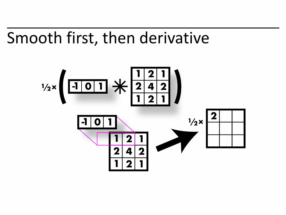
Smooth first, then derivative

Smooth first, then derivative

Smooth first, then derivative

Smooth first, then derivative

Smooth first, then derivative

Smooth first, then derivative

Smooth first, then derivative
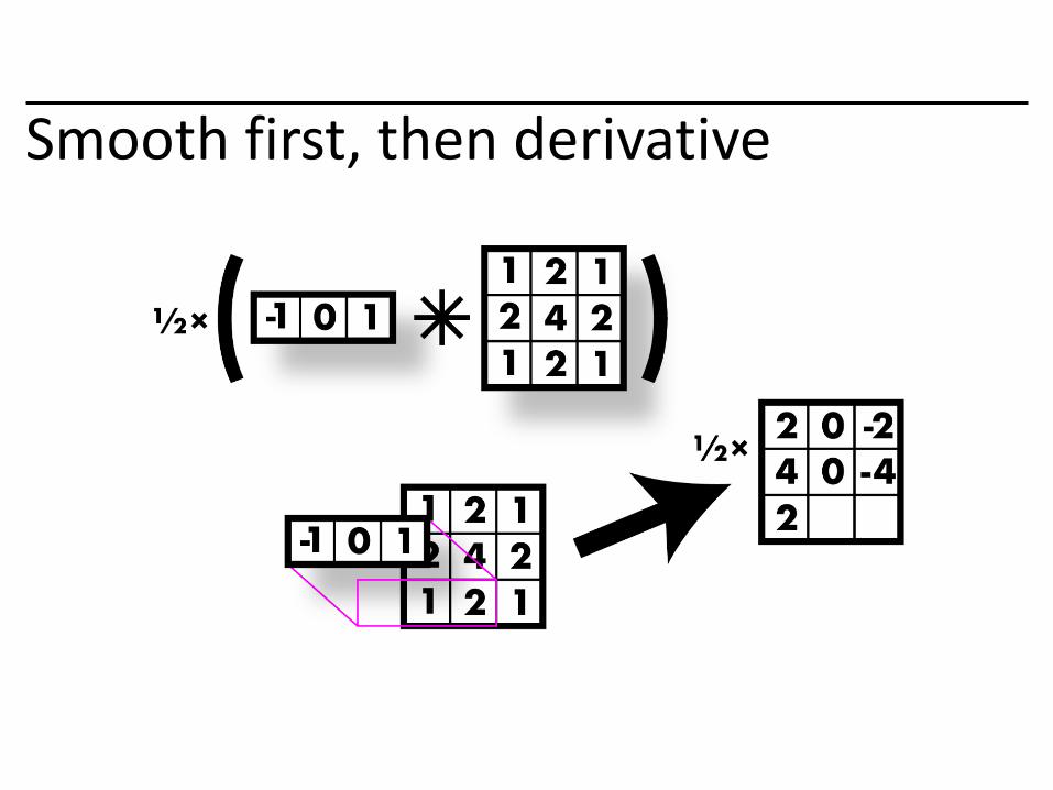
Smooth first, then derivative

Smooth first, then derivative

Smooth first, then derivative

Sobel filter! Smooth & derivative

2nd derivative!- Crosses zero at extrema

Canny Edge Detection- Your first image processing pipeline!
- Old-school CV is all about pipelines
Algorithm:
- 1. Smooth image (only want “real” edges, not noise)- 2. Calculate gradient direction and magnitude- 3. Non-maximum suppression perpendicular to edge- 4. Threshold into strong, weak, no edge- 5. Connect together components
http://bigwww.epfl.ch/demo/ip/demos/edgeDetector/
Canny Characteristics
• The Canny operator gives single-pixel-wide images with good continuation between adjacent pixels
• It is the most widely used edge operator today; no one has done better since it came out in the late 80s. Many implementations are available.
• It is very sensitive to its parameters, which need to be adjusted for different application domains.
25

Canny on Kidney
26

An edge is not a line...
How can we detect lines ?
27

Finding lines in an image
• Option 1:
– Search for the line at every possible position/orientation
– What is the cost of this operation?
• Option 2:
– Use a voting scheme: Hough transform
28

• Connection between image (x,y) and Hough (m,b) spaces– A line in the image corresponds to a point in Hough
space– To go from image space to Hough space:
• given a set of points (x,y), find all (m,b) such that y = mx + b
x
y
m
b
m0
b0
image space Hough space
Finding lines in an image
29

Hough transform algorithm• Typically use a different parameterization
– d is the perpendicular distance from the line to the origin
– is the angle of this perpendicular with the horizontal.
30

Hough transform algorithm• Basic Hough transform algorithm
1. Initialize H[d, ]=0
2. for each edge point I[x,y] in the image
compute gradient magnitude m and angle
H[d, ] += 1
3. Find the value(s) of (d, ) where H[d, ] is maximum
4. The detected line in the image is given by
Complexity? How do you get the lines out of the matrix?
31
d
Array H

Line segments from Hough Transform
32

Extensions• Extension 1: Use the image gradient (we just did that)
• Extension 2
– give more votes for stronger edges
• Extension 3
– change the sampling of (d, ) to give more/less resolution
• Extension 4
– The same procedure can be used with circles, squares, or any other shape, How?
• Extension 5; the Burns procedure. Uses only angle, two different quantifications, and connected components with votes for larger one.
33

Finding lung nodules (Kimme & Ballard)
34

K-Means Clustering
Form K-means clusters from a set of n-dimensional vectors
1. Set ic (iteration count) to 1
2. Choose randomly a set of K means m1(1), …, mK(1).
3. For each vector xi compute D(xi , mk(ic)), k=1,…Kand assign xi to the cluster Cj with nearest mean.
4. Increment ic by 1, update the means to get m1(ic),…,mK(ic).
5. Repeat steps 3 and 4 until Ck(ic) = Ck(ic+1) for all k.
35

Simple Example
INIT.
0
1
2
3
4
5
6
7
8
9
10
0 1 2 3 4 5 6 7 8 9 10
0
1
2
3
4
5
6
7
8
9
10
0 1 2 3 4 5 6 7 8 9 10
0
1
2
3
4
5
6
7
8
9
10
0 1 2 3 4 5 6 7 8 9 10
0
1
2
3
4
5
6
7
8
9
10
0 1 2 3 4 5 6 7 8 9 10
0
1
2
3
4
5
6
7
8
9
10
0 1 2 3 4 5 6 7 8 9 10
K=2
Arbitrarily choose K objects as initial cluster center
Assign each object to most similar center
Update the cluster means
Update the cluster means
reassignreassign

Space for K-Means
• The example was in some arbitrary 2D space
• We don’t want to cluster in that space.
• We will be clustering in gray-scale space or color space.
• K-means can be used to cluster in any n-dimensional space.

K-Means Example 1
38

K-Means Example 2
39

K-Means Example 3
40

K-Means Example 4
41
Published in 2006 IEEE Southwest Symposium on Image Analysis and Interpretation 2006Medical Image Segmentation Using K-Means Clustering and Improved Watershed AlgorithmH. P. Ng, S. Ong, K. Foong, P. Goh, W. Nowinski

K-Means Example 5
42
Published in 2006 IEEE Southwest Symposium on Image Analysis and Interpretation 2006Medical Image Segmentation Using K-Means Clustering and Improved Watershed AlgorithmH. P. Ng, S. Ong, K. Foong, P. Goh, W. Nowinski

K-Means Example 5
• Superpixel clustering in breast biopsy images
43
benign atypia DCIS

K-means Variants
• Different ways to initialize the means
• Different stopping criteria
• Dynamic methods for determining the right number of clusters (K) for a given image
• The EM Algorithm: a probabilistic formulation of K-means
44

Blobworld: Sample Resultsusing color, texture, and EM
45

Semantic Segmentation
• Instead of grouping pixels based on color, texture or whatever properties
• Teach a classifier what important regions look like, so it can find them.
• This is usually done via deep learning, which we will discuss later in the course.
• But here’s a preview.
46

Training Labels
47
background benign epithelium
malignant epithelium
normal stroma
desmoplastic stroma
secretion
blood
necrosis

Meaning of Labels
• Benign Epithelium: epithelial cells from the benign and atypia categories
• Malignant Epithelium: epithelial cells from DCIS and invasive cancer
• Normal Stroma: normal connective tissue
• Desmoplastic Stroma: stroma associated with a tumor
• Secretion: benign substance filling the ducts
• Necrosis: dead cells at the center of the ducts in DCIS and invasive cases
• Blood: blood cells
• Background: empty areas inside ducts
48

Superpixel + SVM-based Segmentation
49
color and texture histograms
no neighborhood 1 neighborhood 2 neighborhoods
background benign epithelium
malignant epithelium
normal stroma
desmoplastic stroma
secretion
blood
necrosis
Ground Truth

50
CNN-based Segmentation384 × 384
256 × 256
Input Image
Encoder-DecoderEncoder-Decoder
Segmentation
256 ×256
PlainGround Truth Multi-Resolution
background benign epithelium
malignant epithelium
normal stroma
desmoplastic stroma
secretion
blood
necrosis

Supervised Tissue Label Segmentation
• Each superpixel is assigned a class label.
• Context: Two circular neighborhoods
• Relatively simple model
• Faster to train (~3 hours)
• Each pixel is assigned a class label.
• Context: 256x256 and 384x384 pixel patches
• More complex model
• ~1 week to train on special hardware
51
Superpixel + SVM CNN
52
0.0
0.2
0.4
0.6
0.8
1.0
bac
kgro
un
d
ben
ign
ep
i
mal
ign
ant
epi
no
rmal
str
om
a
des
mo
pla
stic
str
secr
etio
n
blo
od
nec
rosi
s
Precision
0.0
0.2
0.4
0.6
0.8
1.0
bac
kgro
un
d
ben
ign
ep
i
mal
ign
ant
epi
no
rmal
str
om
a
des
mo
pla
stic
str
secr
etio
n
blo
od
nec
rosi
s
Recall
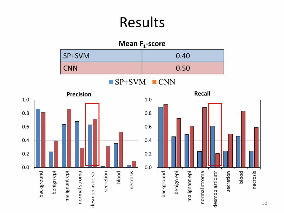
Mean F1-score
SP+SVM 0.40
CNN 0.50
Results

.89 .01 .01 .00 .02 .07 .00 .01
.02 .27 .31 .03 .27 .08 .00 .02
.02 .10 .47 .00 .24 .16 .00 .00
.05 .01 .06 .28 .35 .19 .04 .03
.04 .03 .17 .03 .61 .11 .00 .01
.04 .02 .07 .27 .14 .20 .21 .05
.03 .01 .05 .13 .23 .05 .46 .04
.12 .04 .13 .00 .26 .20 .01 .24
Confusion Matrices
53
Superpixels + SVM CNN

Segmentation Results
54
RGB SVM PredictionsGround Truth Labels CNN Predictions
background benign epi malignant epinormal stroma desmoplastic stromasecretion bloodnecrosis

Segmentation Summary
• Tissue-label segmentation is a useful abstraction.
• We developed a set of 8 tissue labels and collected pixel-label data from a pathologist on 58 ROIs.
• We trained two models: SVM and CNN
• CNNs performed significantly better than SVMs both quantitatively and qualitatively.
55