Embed Size (px)
Citation preview

1
Midterm Supply Chain Planning Under Demand Uncertainty :
Customer Demand Satisfaction and Inventory Management
Anshuman Gupta and Costas D. Maranas1
Department of Chemical Engineering, The Pennsylvania State University
University Park, PA 16802
Conor M. McDonald
Dupont Lycra
Barley Mill Plaza, BMP25-2361
Wilmington, Delaware 19880-0025
1 Author to whom all correspondence should be addressed. E-mail:[email protected]. Phone:814-863-9958. Fax: 814-865-7846

2
Abstract
This paper utilizes the framework of midterm, multisite supply chain planning under demand uncertainty
(Gupta and Maranas, 2000) to safeguard against inventory depletion at the production sites and excessive
shortage at the customer. A chance constraint programming approach in conjunction with a two-stage
stochastic programming methodology is utilized for capturing the trade-off between customer demand
satisfaction (CDS) and production costs. In the proposed model, the production decisions are made before
demand realization while the supply chain decisions are delayed. The challenge associated with obtaining
the second stage recourse function is resolved by first obtaining a closed-form solution of the inner
optimization problem using linear programming duality followed by expectation evaluation by analytical
integration. In addition, analytical expressions for the mean and standard deviation of the inventory are
derived and used for setting the appropriate CDS level in the supply chain. A three-site example supply
chain is studied within the proposed framework for providing quantitative guidelines for setting customer
satisfaction levels and uncovering effective inventory management options. Results indicate that
significant improvement in guaranteed service levels can be obtained for a small increase in the total cost.
3
Introduction
Product demand variability can be identified as one of the key sources of uncertainty in any supply chain.
Failure to account for significant product demand fluctuations in the medium term (1-2 years) by
deterministic planning models may either lead to excessively high production costs (translating to high
inventory charges) or unsatisfied customer demand and loss of market share. Recognition of this fact has
motivated significant work aimed at studying process planning and scheduling under demand uncertainty.
Specifically, most of the research on this problem has largely focussed on short term scheduling of batch
plants (Shah and Pantelides, 1992; Ierapetritou and Pistikopoulos, 1996; Petkov and Maranas, 1998) and
long term capacity planning of chemical processes (Clay and Grossmann, 1994; Liu and Sahinidis, 1996).
Some of the important features that have not been considered in great detail include (semi)continuous
processes, multisite supply chains and midterm planning time frames. In view of this, incorporation of
demand uncertainty in midterm planning of multisite supply chains having (semi)continuous processing
attributes is discussed in Gupta and Maranas (2000) through a two-stage stochastic programming
framework. In this paper, the trade-off involved between inventory depletion and production costs in the
face of uncertainty is captured in a probabilistic framework through chance-constraints. A customized
solution technique, aimed at reducing the computational expense typically associated with stochastic
optimization problems, is developed. The basic idea of the proposed methodology consists of translating
the stochastic attributes of the problem into an equivalent deterministic form which can be handled
efficiently.
The rest of the paper is organized as follows. In the next section, the two-stage stochastic model, which is
based on the deterministic midterm planning model of McDonald and Karimi (1997), is presented. Next,
the key elements of the proposed solution methodology are discussed briefly. The details of the analysis
can be found in Gupta and Maranas (2000). The main part of the paper proposes a chance-constraint
based approach for capturing the trade-off between customer shortage and production costs. The other
critical issue of excessive inventory depletion is then addressed within the proposed framework by
obtaining analytical expressions for the mean and standard deviation of the inventory. These are utilized
for setting the appropriate service level in the supply chain. Computational results for an example supply
chain are presented followed by concluding comments.
Two-Stage Model
The slot-type economic lot sizing model of McDonald and Karimi (1997) is adopted as the benchmark
formulation for this work. The variables of this model can be partitioned into two categories (Gupta and
Maranas, 2000) based on whether the corresponding tasks need to be carried out before or after demand
realization. The production variables model activities such as raw material consumption, capacity
utilization and final product production. Due to the significant lead times associated with these tasks, they
are modeled as “here-and-now” decisions which need to be taken prior to demand realization. Post

4
production activities such as inventory management and supply of finished product to customer, on the
other hand, can be performed much faster. Consequently, these constitute the supply-chain variables
which can be fine-tuned in a “wait-and-see” setting after realization of the actual demand. This
classification of variables naturally extends to the constraints of the problem (Gupta and Maranas, 2000)
and results in the following two-stage formulation.
≤≤−
≤≤−
−=
≤
+++
=
∆
−
−∆
≥
∑
∑∑∑∑∑−∆
Lisisis
Lis
iis
isi
isisis
is
is
ii
iissi
isissi
isissi
isIIIS
IIII
IS
SAI
S
IIIhSt
EQ
isisisis
i
θθ
θ
µζ
θ
min,,,0,,,
subject to
fjsfjsi
ijsfjsfjs
fjsf i
ijs
siss
jijsisis
ssis
jjsi
iisiis
ijsijsijs
YHRLYMRL
HRL
WPIA
WPC
RLRP
if
if
≤≤
≤
−+=
==
=
∑
∑ ∑
∑∑
∑∑∑
=
=
1:
1:
’’
0
’’’
’’
λ
λ
β
In the above formulation, the various indices are as follows: i(products), f (product families), j (processing
equipment) and s (production sites). The various cost parameters are FCfs (setup cost), νijs (variable
production cost), pis (raw material cost), tiss′ (intersite transportation cost), tis (customer-site transportation
cost), his (inventory holding cost), ζis (safety stock violation penalty) and µi (lost revenue cost). MRLfjs is
the minimum runlength, Hfjs is the total available processing time while Rijs is the rate of production and
βi′is is the material balance coefficient. Other parameters are I0is (initial inventory), IL
is (safety stock level)
and θi (uncertain demand).
The objective function of the above formulation is composed of two terms. The first term, subject to the
outer optimization problem constraints, accounts for the costs incurred in the production stage. Production
stage variables include Ais (availability), Pijs (production amount), RLijs (runlength), Cis (raw material
consumption), Wis’s (intersite shipment) and Yfjs (setup). The second term Q is obtained by applying the
QWtCpPYFC issssi
ississi
isijssji
ijsfjssjf
fs
YWCAFRLRLP
fjs
issisis
fjsijsijs
++++ ∑∑∑∑∈
≥
’’,,
’,,,,,
}1,0{0,,
,,
’
min ν

5
expectation operator to the optimal value of an embedded optimization problem. The constraints of this
inner recourse problem are the supply chain constraints and the inner stage variables, Sis (supply), Iis
(inventory), Iis∆ (safety stock deficit) and Iis
- (customer shortage), are the supply chain variables. The
interaction between the outer (production) and inner (supply chain) problems takes place through the
inventory balance constraint which forces the inventory to be equal to the difference between the amount
available for supply (Ais) and the actual supply to the customer (Sis). The basic idea of the proposed
methodology consists of obtaining a closed-form analytical expression for Q (the recourse function) in
terms of the first stage production variables (specifically Ais). This is achieved by first explicitly solving
the inner recourse problem followed by analytical expectation evaluation (Gupta and Maranas, 2000).
Optimal Supply Policies
The inner supply chain planning problem is solved analytically using linear programming (LP) duality
(Gupta and Maranas, 2000). In particular, the key principle utilized is the strong LP duality theorem. To
aid the developments, some additional notation is introduced. The production sites are classified as either
internally sufficient (IS) or internally deficient (ID) as
{ } { }0ID and 0IS ≤−∈=≥−∈= Lisis
Lisis IASsIASs
Thus, at the ID sites, safety stock violation cannot be avoided as the amount available for supply is not
adequate to meet the safety stock requirement. Two additional cost parameters, the over-safety stock
supply cost (γis) and the under-safety stock supply cost (ωis), are introduced. These are given by
isisisisisisis htht ζωγ +−=−= and
These represent per unit costs of shipping a product from above (γis) or below (ωis) the safety stock level.
Ranking of the IS and/or ID sites on the basis of these cost parameters forms the key principle of the
proposed methodology. By exploiting the network representation of the inner supply chain planning
problem, three distinct demand regimes are uncovered in the optimal solution. These are referred to as
regimes of low, intermediate and high demand realizations. A summary of the supply policies for these
demand regimes is provided below.
Low Demand Regime
In this demand regime, the safety stock violation penalty is restricted to the ID sites by directing all
customer product supply from the IS sites. Ranking of the IS sites in increasing order of over-safety stock
supply cost (γis) represents the optimal sequence in which the sites service the customer. Therefore, for an
IS site sl* with
( ) ( )∑∑∈=
−
∈=
−≤≤−**
1
1
1
ll s
ISss
Lisisi
s
ISss
Lisis IAIA θ
the optimal supply policies are given by

6
( )
∈∀∈+≥∀
∈=∀−−
∈−≤∀−
= ∑−
∈=
and,10
,
,1
*
1
1
*
*
*
IDsISsss
ISsssIA
ISsssIA
S
l
s
ISss
lLisisi
lLisis
is
l
θ
Note that given the optimal supply policies, the optimal values for the remaining supply chain variables
can be calculated (for any demand regime) as:
( )
−=−=−= ∑−∆
sisiiis
Lisisisisis SIIIISAI θ,0max;,0max;
No safety stock violations occur at any of the IS sites and no sales are lost in this demand regime. The
transition to the intermediate demand regime occurs at a demand realization given
by ( )∑∈
→ −=ΘISs
Lisis
ILi IA
Intermediate Demand Regime
In the intermediate demand regime, the entire customer demand is met only at the expense of incurring
safety stock violation penalties at some or all of the production sites. Consequently, all sites are ranked in
increasing order of under-safety stock supply cost (ωis) irrespective of their type (i.e., IS or ID). This
establishes the order in which demand is allocated to the production sites in the intermediate demand
regime. For a site si* defined as
∑∑∑∑∈=
∈=
→−
∈=
−
∈=
→ ++Θ≤≤++Θ****
11
1
1
1
1
iiii s
ISss
Lis
s
IDss
isIL
ii
s
ISss
Lis
s
IDss
isIL
i IAIA θ
the corresponding optimal supply policies are
( )
∈+≥∀−
∈+≥∀
=∀−−−
−≤∀
=∑ ∑
−
=∈
+≥
ISsssIA
IDsss
ssIAA
ssA
S
iLisis
i
i
s
sISs
ss
Lisisisi
iis
is
i
i
,1
,10
1
*
*
*1
1 1
*
*
*
θ
As in the low demand regime, no shortfall occurs at the customer. Transition to the high demand regime
occurs at the demand realization given by ∑=Θ →
sis
HIi A

7
High Demand Regime
In this demand regime, due to high levels of customer demand, the entire amount available for supply is
shipped to the customer following the “customer priority” paradigm (Gupta and Maranas, 2000).
Therefore, for ∑≥s
isi Aθ the optimal supply policies are given by
sAS isis ∀=
Inventories at all the sites are completely depleted resulting in maximum safety stock violation charges.
The high demand regime is unique in the sense that it is the only regime in which unsatisfied demand
occurs at the customer and the inventory at all the sites is zero.
After solving the inner problem explicitly, the recourse function Q is calculated by integrating the optimal
objective value over all possible demand realizations. This undertaking translates into the calculation of
three conditional probability integrals, one for each of the three demand regimes. Consequently, by
invoking the normality assumption for the product demands followed by analytical integration, the
following form for the recourse function is obtained (for details see Gupta and Maranas, 2000).
( ) ( )[ ]∑ ∑ +Φ+=si si
isisisiisisis KfKKbKaQ, ,
σ
where ais, bis are constants which are functions of the second stage cost parameters, σi is the standard
deviation of the demand, f( ) and Φ( ) are the normal density and cumulative distribution functions
respectively and
( )i
miis
is
AK
σθ−=
with θ im as the mean demand.
Customer Demand Satisfaction
Missed sales in the high demand regime are unacceptable from a customer relationship perspective given
the constant shifting of customer loyalties in today’s highly competitive business environment. Therefore,
to safeguard against this scenario in a probabilistic framework, the following chance constraint is
introduced.
αθ ≥
=Θ≤ ∑→
sis
HIii APr
where α is the target customer demand satisfaction (CDS) level. This constraint ensures that the
probability of operating the supply chain in the high demand regime is less than (1-α). By changing the
value of α, optimal trade-off curves can be constructed between total cost and frequency of missed
customer demand. The deterministic equivalent form for the chance constraint is obtained as
( )ασθ 1−Φ+≥∑ imi
sisA

8
where Φ-1( ) is the inverse normal cumulative distribution function. The stochastic attributes of the
original problem are thus transformed into (exact) equivalent deterministic form resulting in a convex
nonlinear mixed integer programming problem (Gupta and Maranas, 2000).
Inventory Control
In addition to lost sales, the high demand regime is also characterized by depletion of inventory in the
entire supply chain for a particular product. This could pose significant operational challenges. Even
though the chance constraint introduced to limit customer shortage favorably affects the inventory
profiles in the supply chain by increasing the amount available for supply, the problem of inventory
depletion at a production site is not completely resolved. Excessively low inventory levels at individual
sites might still occur as the chance constraint only relates the aggregate amount available in the supply
chain to the CDS level. Consequently, a more robust operation of the supply chain from an inventory
management perspective can be achieved by studying the variation of the probability distribution and the
corresponding mean and standard deviation of the inventory level with changing CDS targets. For this
undertaking, analytical expressions relating the expected level and standard deviation of the inventory to
the amount available for supply at each production site are developed. By applying the expectation
operator to the inventory balance constraint, the average inventory can be related to the expected supply
as
[ ] [ ]isisis SEAIEii θθ −=
By conditionally integrating the supply policies presented in the previous section and substituting in the
above equation, the mean inventory is obtained as
[ ] ( ) ( )[ ]( ) ( )[ ]( ) ( )[ ]( ) ( )[ ]
1,1,1,
1,1,1,
,,,
,,,
222
111
222
111
−=−=−=
−=−=−=
===
===
+Φ−
+Φ−
+Φ+
+Φ=
Is
Is
Is
Ls
Ls
Ls
Is
Is
Is
Ls
Ls
Lsi
rsirsirsii
rsirsirsii
rsirsirsii
rsirsirsiiis
KfKK
KfKK
KfKK
KfKKIE
σ
σ
σ
σθ
where
( )
i
s
ISss
mi
Lisis
is
l
IA
Kσ
θ∑∈=
−−
=
*
1
1
i
mi
s
ISss
Lis
s
IDss
isIL
i
is
ii
IA
Kσ
θ−++Θ
=
∑∑∈=
∈=
→**
11
2

9
and rsL and rs
I are the ranks of site s in the low and intermediate demand regimes respectively. An
interesting observation can be made based on the expression for the mean inventory. Convexity of the
( ) ( )KfKK +Φ terms implies that the mean inventory is the sum of convex (first two) and concave (last
two) terms. In the light of this observation, oscillations in the expected inventory level due to the change
in relative magnitudes of these two components, might be expected. This trend is actually observed in the
supply chain example studied later in the paper.
In addition to the expected inventory, the standard deviation of the inventory distribution can also be
calculated within the analytical framework. By squaring the inventory balance constraint followed by
conditional expectation evaluation, the following expression for the inventory standard deviation is
obtained.
[ ] [ ] [ ] [ ]22isisisis IEIEIVarISD
ii θθ −==
where
[ ] ( )( ) ( )[ ] ( )[ ]
( ) ( )[ ][ ] ( ) ( )[ ]
( ) ( )[ ]( )
( ) ( )[ ] ( )[ ]( ) ( )[ ]
[ ] ( ) ( )[ ]1,,1,
1,1,,,
2
22
1,1,,
2
,1,
1,,1,
1,1,,,
2
22
1,1,,
2
1,
2
2222
2222
212
12
1112
1111
111
1
−==−=
−=−===
−=−==
=−=
−==−=
−=−===
−=−==
−=
−++
−−
++Φ−Φ+
Φ−Φ+
−++
−−
++Φ−Φ+
Φ=
Is
Is
Is
Is
Is
Is
Is
Is
Is
Is
Ls
Is
Ls
Ls
Ls
Ls
Ls
Ls
Ls
Ls
Ls
Ls
Lsi
rsirsirsiiLisi
rsirsirsirsii
irsiiLisrsirsi
Lisrsirsi
rsirsirsiiisi
rsirsirsirsii
irsiiisrsirsi
isrsiis
KfKfKI
KfKKfK
KIKK
IKK
KfKfKA
KfKKfK
KAKK
AKIE
σσ
σ
σσ
σσ
σ
σσ
θ
The above result is based on the following conditional expectation results.
[ ] ( )( )1
11112
K
KfKKzzE z Φ
−=≤
[ ] ( ) ( )( )( ) ( )( )12
11221212
KK
KfKKfKKzKzEz Φ−Φ
−−=≤≤
where z follows a standard normal distribution N(0,1). By studying the variation in the mean and standard
deviation of inventory levels at the various production sites with changing CDS levels, the choice of the
appropriate service level can be further refined to account for inventory depletion.

10
Example
The proposed methodology is highlighted through a three-site example supply chain illustrated in Figure
1. A total of 10 products, grouped into 5 product families, are manufactured at these facilities, which are
characterized by different processing and cost attributes. Each site has single processing equipment
dedicated for each product family and the products within the family compete for the limited capacity of
this equipment. Setup charges are incurred for each production campaign and product demand exists at a
single customer. The data for the example is given in Tables 1 through 3.
First, the deterministic midterm planning problem is solved. This yields an optimal solution of 4,165.
Subsequently, the deterministic equivalent problem under uncertainty is solved without enforcing the
chance constraints. Solution of this convex MINLP using DICOPT accessed via GAMS, results in an
optimal expected cost of 4,726 obtained in 43 CPU seconds. The model consists of 301 constraints, 286
continuous variables and 75 discrete variables and is solved to optimality in 9 iterations. The difference
between the deterministic and stochastic solutions quantifies the impact of uncertainty in the supply
chain. The values obtained are verified, at considerably higher computational expense, by solving the
same problem instance with Monte Carlo (MC) sampling. Comparison of computational requirements
(2038 CPU seconds for MC with 500 sampled scenarios as compared to 43 CPU seconds) highlights the
efficiency of the proposed methodology.
Customer Demand Satisfaction
Given this “base” production setting for the supply chain, the “base” CDS level is calculated for each
product (Figure 2). This represents the probability that the demand realized for a particular product lies
either in the low or the intermediate demand regime. Equivalently, it is the probability that no customer
orders are lost. As the figure indicates, CDS levels ranging from 70% to 80% are achieved with the base
production plan. Next, the chance constraint is introduced into the problem and the problem is solved for
varying CDS target levels. The optimal total costs thus incurred are shown in Figure 3. As illustrated in
the figure, the total cost increases relatively linearly with the CDS level. This initial linear relation,
however, changes to an exponential one at CDS levels ranging from 90-97%. This implies that at the
expense of modest cost increase, the customer demand satisfaction can be improved to about 90-97%.
Also, the continuously increasing slope of the curve implies that the cost incurred per unit change in CDS
level increases with the CDS level. This is expected in the light of the classic law of diminishing returns.
To gain further insight into the operation of the supply chain with respect to varying levels of CDS, the
total cost incurred is analyzed in terms of its deterministic (first stage production costs) and stochastic
(second stage supply costs) components. The resulting trade-off curve obtained is shown in Figure 4. As
the CDS target level is increased, the expected supply chain costs decrease as the largest component of
this cost, the lost revenue, is reduced. The production costs, on the other hand, increase primarily because

11
of the additional setups required for increasing the amount available for supply. For a unit increase in the
production costs, the reduction in the supply chain costs is approximately 60%. This is in agreement with
the observation that the total cost increases with increasing CDS level (Figure 3). The difference between
the additional production costs and the resulting supply chain savings can be viewed as the cost incurred
for making the supply chain more robust and reliable from a customer service viewpoint. As shown in
Figure 4, the expected supply chain savings level off in the range of 95-97% CDS level, which is
approximately the level at which the total cost starts increasing exponentially (Figure 3).
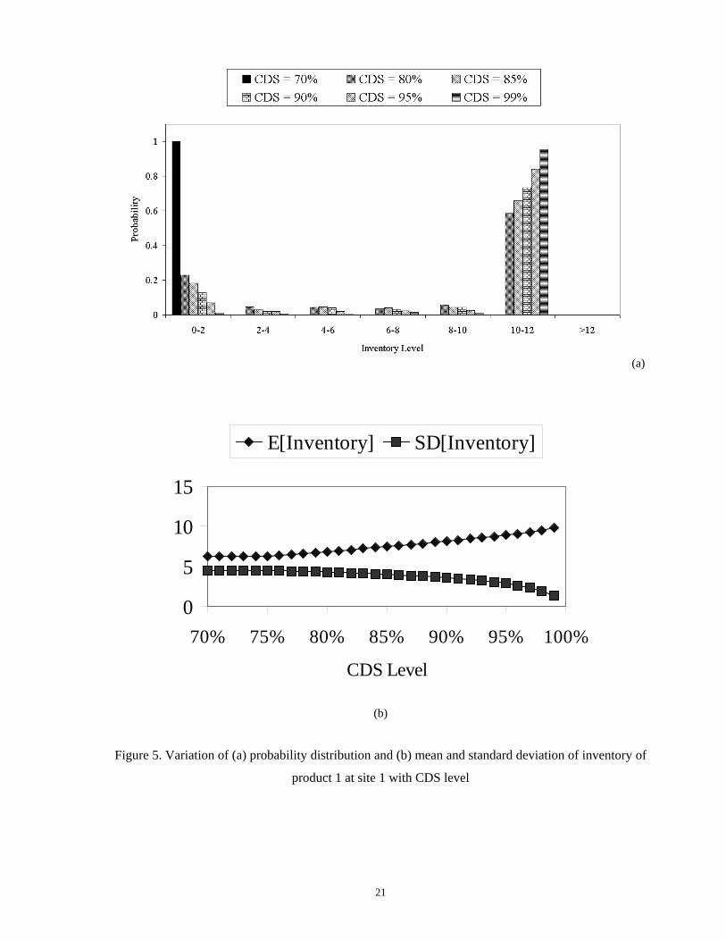
Inventory Control
Having addressed customer shortage management through the chance constraint, the issue of inventory
control in the supply chain is considered. The variations of the probability distributions, corresponding
expected values and standard deviations of the inventory of product 1, with changing CDS levels are
shown in Figure 5 through Figure 7. At site 1, the probability of having the inventory at the safety stock
level of 10 units is relatively high even for low CDS levels (Figure 5(a)). This probability increases with
increasing CDS level as more product is made available for supply. The expected inventory
correspondingly increases with the CDS level while the standard deviation decreases as shown in Figure
5(b). Thus, with respect to inventory management considerations at site 1, a high CDS level would be
preferred as this would translate into high levels of inventory with lower variability. The inventory
distribution at site 2 is considerably more depleted than in site 1 (Figure 6(a)) as the probability of having
low inventory is relatively high even at high CDS levels. For instance, there is approximately 50%
probability of completely depleting inventory at a CDS level as high as 99%. However, the expected
inventory profile at site 2 in Figure 6(b) indicates average inventory levels in the range of 6-7 units
between CDS levels of 70-80%. These values are misleading when viewed in light of the actual
probability distribution of the inventory. They can be attributed to extremely high inventory levels (30-40
units) existing at very low probability levels (0.05-0.1) at site 2. This is also reflected in the high standard
deviation (8-9 units) of the inventory level in this CDS level range. Almost complete inventory depletion
is predicted at site 2 in CDS levels ranging from 80-90%. This trend is followed by significant cyclical
variations in expected inventory with increasing CDS level coupled with correlated variations in the
corresponding standard deviation. These oscillations can be attributed to the changing relative magnitudes
of the convex and concave terms in the expression for the expected inventory. At site 3, complete
inventory depletion can be predicted with 100% probability for CDS levels ranging from 70% to 80% as
shown in Figure 7(a). This observation is also supported by the expected inventory profile in Figure 7(b).
Average inventory of 8-9 units with a corresponding standard deviation of 8-9 units is expected to occur
between 80-90% CDS level. The high standard deviation is also indicated by the probability distribution
in this range of CDS values as most of the inventory levels that can occur are approximately equally
likely. Cyclical changes similar to site 2 are also observed at site 3 at higher CDS levels.

12
Using these inventory profiles for the three sites, the choice of the “optimal” CDS level at which the
supply chain should operate can be determined. The CDS level range of 90-97% as determined by the
service level considerations can be further refined to effectively account for inventory control issues.
Based on the results indicated in Figures 5 through 7, an appealing CDS level to operate the supply chain
at is 97%. The expected inventories at sites 1, 2 and 3 at this CDS level are approximately 9 units, 6 units
and 13 units respectively. The corresponding supply chain and production costs are 2,041 and 3,011
respectively (5,052 total cost). Therefore, an improvement of 17% in the CDS level is achieved over the
base setting at the expense of 7% additional cost.
Hedging Inventory Risk
An interesting observation that can be made by comparing the inventory profiles at site 2 (Figure 6(b))
and site 3 (Figure 7(b)) is that the inventory variations are complementary at the two sites. Low expected
inventory at one site corresponds to high levels at the other. This trend is also incorporated in the cyclical
fluctuations in the high CDS range where the oscillations at the two sites are “out-of-phase’’. Similar
trends are also seen for the standard deviation of the inventory. This observation can be potentially
utilized for modifying the risk profile of the inventory in the supply chain. By considering the option of
integrating the manufacturing capacity of product 1 at sites 2 and 3, the inventory risk as characterized by
the standard deviation can be effectively “squeezed’’ out from the system. The corresponding hedged
position is shown in Figure 8. Smoother inventory profiles in conjunction with relatively constant
standard deviation can make the operation of the supply chain more robust.
Summary
In this paper, a two-stage modeling framework coupled with a chance constraint programming approach
was utilized for incorporating demand uncertainty and issues of customer demand satisfaction and
inventory management. In addition, inventory depletion in multisite supply chains was addressed within
the proposed analytical framework. The customized solution procedure for the two-stage problem (Gupta
and Maranas, 2000) was extended to account for the probabilistic constraints introduced to enforce
desired customer demand satisfaction levels. Analytical expressions for the mean and standard deviation
of the inventory levels at the various production sites were used for making the supply chain more robust
from an inventory management perspective. The fact that significant improvements in terms of
guaranteed service levels to the customer could be achieved at relatively small additional cost was
indicated through an example supply chain planning problem. The possibility of uncovering potential
strategic options for managing inventory risk in the supply chain was also highlighted.
Acknowledgements
The authors gratefully acknowledge financial support by the NSF-GOALI Grant CTS-9907123 and
DuPont Educational Aid Grant 1999/2000.

13
References Clay, R. L. and Grossmann, I. E., Optimization of stochastic planning models. Trans. IchemE, 72, 415
(1994).
Gupta, A. and Maranas, C. D., A two-stage modeling and solution framework for multisite midterm
planning under demand uncertainty. Accepted for publication in I&EC Research (2000).
Ierapetritou, M. G. and Pistikopoulos, E. N., Batch plant design and operations under uncertainty. I&EC
Research, 35, 772 (1996).
Liu, M. L. and Sahinidis, N. V., Optimization in process planning under uncertainty. I&EC Research, 35,
4154 (1996).
McDonald, C. and Karimi, I. A., Planning and scheduling of parallel semicontinuous processes. 1.
Production planning. I&EC Research, 36, 2691 (1997).
Petkov, S. B. and Maranas, C. D., Design of single-product campaign batch plants under demand
uncertainty. AIChE Journal, 44, 896 (1998).
Shah, N. and Pantelides, C. C., Design of multipurpose batch plants with uncertain production
requirements. I&EC Research, 31, 1325 (1992).

14
Table 1. Family dependent production parameters for the example supply chain
Site(s) Product Family (f) Fixed Cost (FCfs) Minimum Runlength (MRLfs) Available Time (Hfs)
1 {1,2,3,4,5} {4.5,4.8,5.5,6.2,4.5} {75,75,75,75,75} {150,250,200,185,190}
2 {1,2,3,4,5} {6.5,3.5,6.5,4.5,6.5} {75,75,75,75,75} {250,200,150,200,190}
3 {1,2,3,4,5} {6.5,5.2,5.1,4.7,6.5} {50,50,50,50,50} {225,270,250,150,265}

15
Table 2. Cost parameters for the example problem
Parameter s=1 s=2 s=3
Production Cost (νis) 2.5 2.3 2.6
Transportation Cost (tis) 1.1 1.2 1.3
Inventory Cost (his) 1.8 1.7 1.6
Underpenalty Cost (ζis) 2.7 2.3 2.2
Production Rate (Ris) 0.5 0.6 0.5
Initial Inventory (I0is) 0 0 0
Safety Stock Level (ILis) 10 15 25

16
Table 3. Demand distributions and revenues for the products
Product
(i)
Demand
(θi)
Revenue
(µi)
1 N(70,15) 10.0
2 N(50,10) 9.0
3 N(85,10) 9.5
4 N(100,30) 10.5
5 N(100,20) 9.0
6 N(90,20) 11.0
7 N(55,15) 10.8
8 N(80,20) 10.0
9 N(95,30) 12.0
10 N(110,25) 8.5

17
Figure 1. Three-site example supply chain

18
Figure 2. Base customer demand satisfaction levels in the supply chain
60%
65%
70%
75%
80%
85%
1 2 3 4 5 6 7 8 9 10
Products
Bas
e C
usto
mer
Dem
and
Sat
isfa
ctio
n L
evel

19
4600
4700
4800
4900
5000
5100
5200
5300
80% 85% 90% 95% 100%Customer Demand Satisfaction Level
Tot
al C
ost
Figure 3. Variation of total cost with customer demand satisfaction level (α )

20
α=87%α=85%
α=83%
α=99%α=97%α=95%
α=91%α=89%
α=81%
α=79%
α=76%
2000
2100
2200
2300
2400
2400 2500 2600 2700 2800 2900 3000 3100 3200 3300
Production Costs
Exp
ecte
d S
uppl
y C
hain
Cos
ts
Figure 4. Trade-off curve between expected supply chain costs and production costs
21
(a)
0
5
10
15
70% 75% 80% 85% 90% 95% 100%
CDS Level
E[Inventory] SD[Inventory]
(b)
Figure 5. Variation of (a) probability distribution and (b) mean and standard deviation of inventory of
product 1 at site 1 with CDS level

22
(a)
0
5
10
15
70% 75% 80% 85% 90% 95% 100%
CDS Level
E[Inventory] SD[Inventory]
(b)
Figure 6. Variation of (a) probability distribution and (b) mean and standard deviation of inventory of
product 1 at site 2 with CDS level

23
(a)
0
5
10
15
20
70% 75% 80% 85% 90% 95% 100%
CDS Level
E[Inventory] SD[Inventory]
(b)
Figure 7. Variation of (a) probability distribution and (b) mean and standard deviation of inventory of
product 1 at site 3 with CDS level

24
05
1015202530
70% 80% 90% 100%
CDS Level
E[Inventory] SD[Inventory]
Figure 8. Hedging inventory risk at sites 2 and 3 by capacity integration

25
List of Captions Table 1. Family dependent production parameters for the example supply chain
Table 2. Cost parameters for the example problem
Table 3. Demand distributions and revenues for the products
Figure 1. Three-site example supply chain
Figure 2. Base customer demand satisfaction levels in the supply chain
Figure 3. Variation of total cost with customer demand satisfaction level (α )
Figure 4. Trade-off curve between expected supply chain costs and production costs
Figure 5. Variation of (a) probability distribution and (b) mean and standard deviation of inventory of
product 1 at site 1 with CDS level
Figure 6. Variation of (a) probability distribution and (b) mean and standard deviation of inventory of
product 1 at site 2 with CDS level
Figure 7. Variation of (a) probability distribution and (b) mean and standard deviation of inventory of
product 1 at site 3 with CDS level
Figure 8. Hedging inventory risk at sites 2 and 3 by capacity integration


![Production Planning Problems with Joint Service-Level ... · uncertainty in midterm production planning. Kazaz [14] studied production planning with random yield and demand using](https://img.pdfslide.net/doc/110x75/5f80ea08dc04363548737ff7/production-planning-problems-with-joint-service-level-uncertainty-in-midterm.jpg)