Migration Patterns Today and the Factors that Influence Them

Migration Patterns Today and the Factors that Influence Them

David A. Plane, Professor

School of Geography and Development

University of Arizona, Tucson

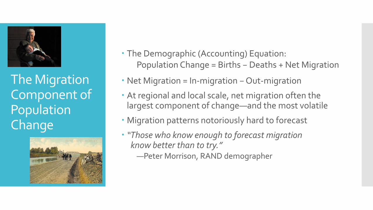
The Migration Component of Population Change

The Demographic (Accounting) Equation:Population Change = Births − Deaths + Net Migration

Net Migration = In-migration − Out-migration

At regional and local scale, net migration often the largest component of change—and the most volatile

Migration patterns notoriously hard to forecast

“Those who know enough to forecast migrationknow better than to try.”

—Peter Morrison, RAND demographer

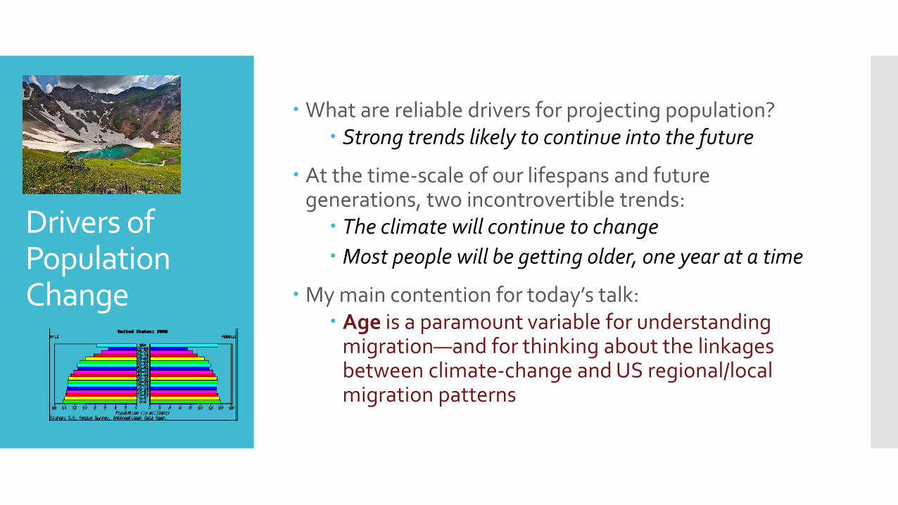
Drivers of Population Change

What are reliable drivers for projecting population? Strong trends likely to continue into the future

At the time-scale of our lifespans and future generations, two incontrovertible trends:

The climate will continue to change

Most people will be getting older, one year at a time

My main contention for today’s talk: Age is a paramount variable for understanding

migration—and for thinking about the linkages between climate-change and US regional/local migration patterns

Migrant streams composed of many differently motivated migrants

At different points in the life course, the reasons to move—and thus the influences on migration— vary widely

Demographic disaggregation is key, yet still myriad reasons why any individual may or may not move

One bifurcation of migration research: Individual/behavioral approaches:

Migration as something people do

Aggregate/geographical approaches: Migration as a reflection of relationships between places and Edward Ullman’s ‘Bases of Spatial Interaction’:

Interregional complementarities

Deterring effect of distance

Intervening opportunities

No such beast as “The Migrant”

Net migration made up of all sorts of people coming into or leaving an area for a plethora of reasons

Complexities of Migration Systems

Many of the influences on migration are highly geographically specific

Plus, migration has a ‘double geography’

Net migration to any particular region or area reflects conditions both there, but also in:

All origins of in-migrants

All potential destinations for out-migrants

At least as challenging to model as climate change!

Migration researchers are like tornado chasers

“Most meteorologists can’t understand it. You have to take a number of factors into account. After a while you develop a feeling for it. Certain patterns appear, points of convergence…

“The atmosphere is a mirror,” he said. “It reflects not only conditions on land, but the temperature and circulation of the ocean currents. When you study the atmosphere, you study everything.”

--William Hauptman, The Storm Season (1992)

So, too, migration is a mirror; when you study migration, you also study everything

Luckily linking climate-change and migration—i.e., everything to everything—is our next speaker’s mission!

My more modest assignment: the current U.S. migration system, and how it, and its influences, play out across regions and local areas

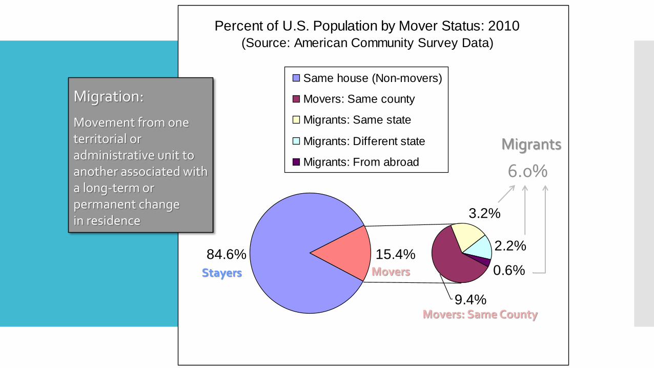
What’s Migration?Percent of U.S. Population by Mover Status: 2010

(Source: American Community Survey Data)

84.6%

3.2%

2.2%

0.6%15.4%

9.4%

Same house (Non-movers)

Movers: Same county

Migrants: Same state

Migrants: Different state

Migrants: From abroad

Stayers Movers

Migrants

6.0%

Migration:

Movement from one territorial or administrative unit to another associated with a long-term or permanent change in residence

Movers: Same County

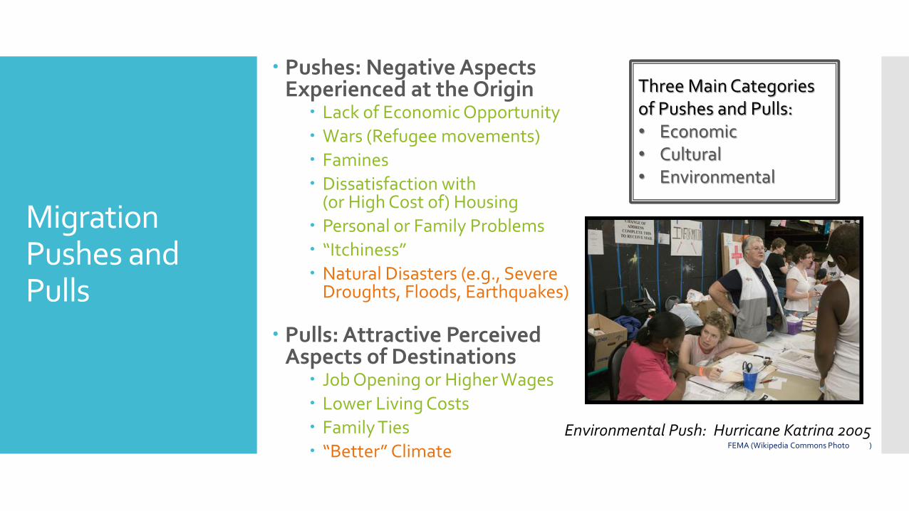
MigrationPushes and Pulls

Pushes: Negative Aspects Experienced at the Origin

Lack of Economic Opportunity

Wars (Refugee movements)

Famines

Dissatisfaction with (or High Cost of) Housing

Personal or Family Problems

“Itchiness”

Natural Disasters (e.g., Severe Droughts, Floods, Earthquakes)

Pulls: Attractive Perceived Aspects of Destinations

Job Opening or Higher Wages

Lower Living Costs

Family Ties

“Better” Climate

Three Main Categories of Pushes and Pulls:• Economic• Cultural• Environmental

Environmental Push: Hurricane Katrina 2005FEMA (Wikipedia Commons Photo )

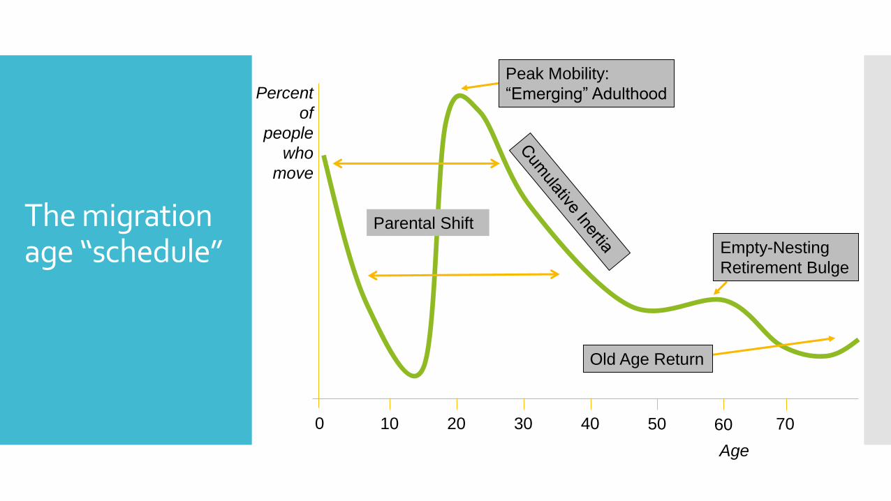
1. The Migration or Mobility “Schedule”

Percent

of

people

who

move

Age

0 10 20 6050 7030 40

Peak Mobility:

“Emerging” Adulthood

Parental Shift

Empty-Nesting

Retirement Bulge

Old Age Return

The migration age “schedule”

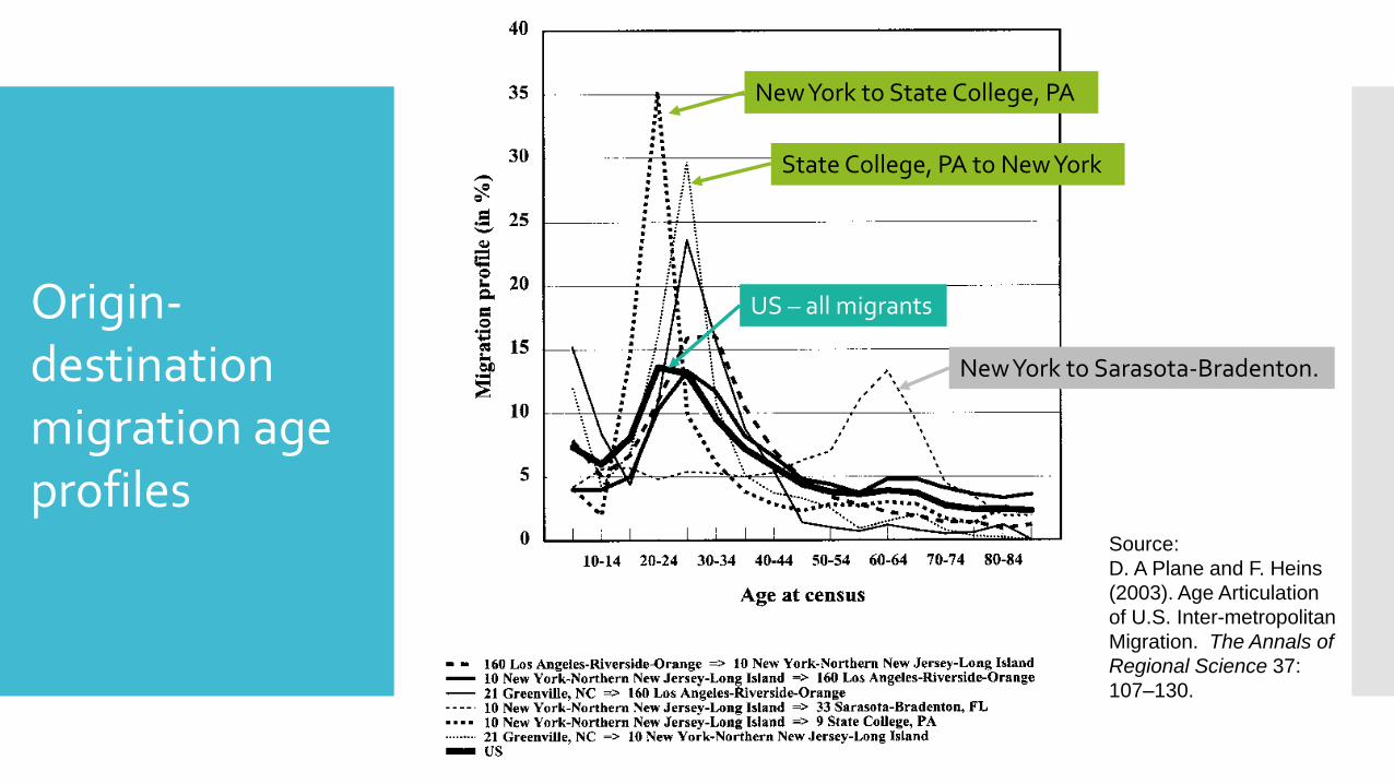
Origin-destination migration age profiles

Source:

D. A Plane and F. Heins

(2003). Age Articulation

of U.S. Inter-metropolitan

Migration. The Annals of

Regional Science 37:

107–130.

New York to State College, PA

State College, PA to New York

US – all migrants

New York to Sarasota-Bradenton.

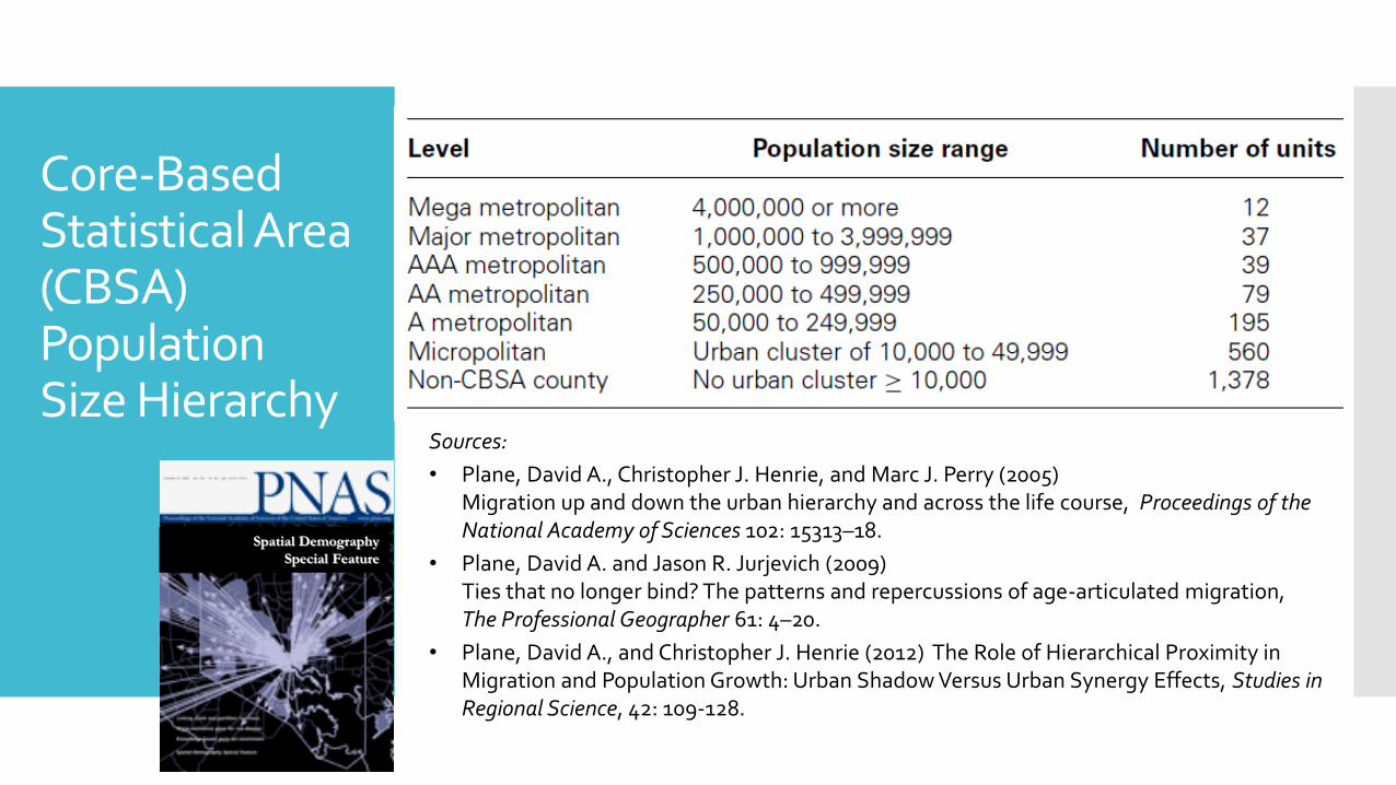
Core-Based Statistical Area (CBSA) Population Size Hierarchy

Sources:

• Plane, David A., Christopher J. Henrie, and Marc J. Perry (2005) Migration up and down the urban hierarchy and across the life course, Proceedings of the National Academy of Sciences 102: 15313–18.

• Plane, David A. and Jason R. Jurjevich (2009) Ties that no longer bind? The patterns and repercussions of age-articulated migration, The Professional Geographer 61: 4–20.

• Plane, David A., and Christopher J. Henrie (2012) The Role of Hierarchical Proximity in Migration and Population Growth: Urban Shadow Versus Urban Synergy Effects, Studies in Regional Science, 42: 109-128.

Spatial Demography

Special Feature

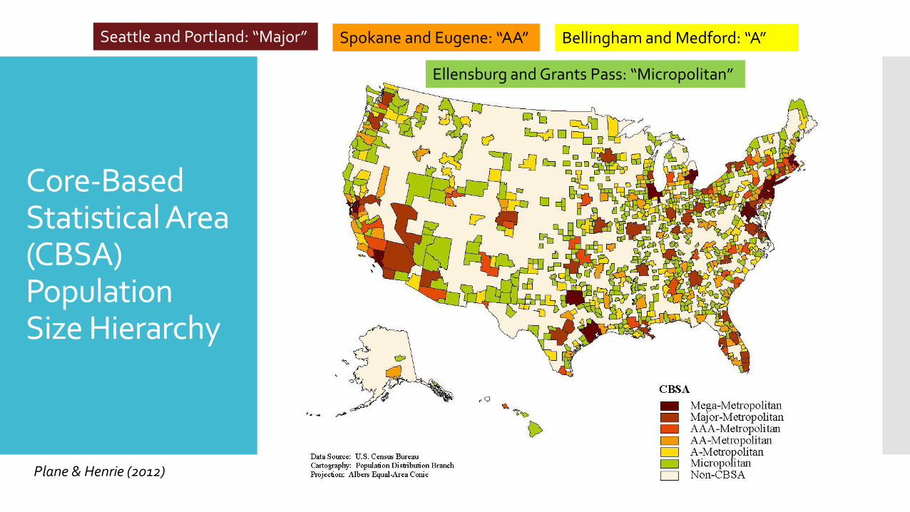
Core-Based Statistical Area (CBSA) Population Size Hierarchy

Plane & Henrie (2012)

Seattle and Portland: “Major” Spokane and Eugene: “AA” Bellingham and Medford: “A”

Ellensburg and Grants Pass: “Micropolitan”

Demographic Effectiveness for Ages 20-29

Flows Up the Hierarchy Flows Down the Hierarchy Legend Mega Metropolitan 2% 10%

Major Metropolitan

5% 25%

AAA Metropolitan

AA Metropolitan

A Metropolitan

Micropolitan

Non-CBSA Counties

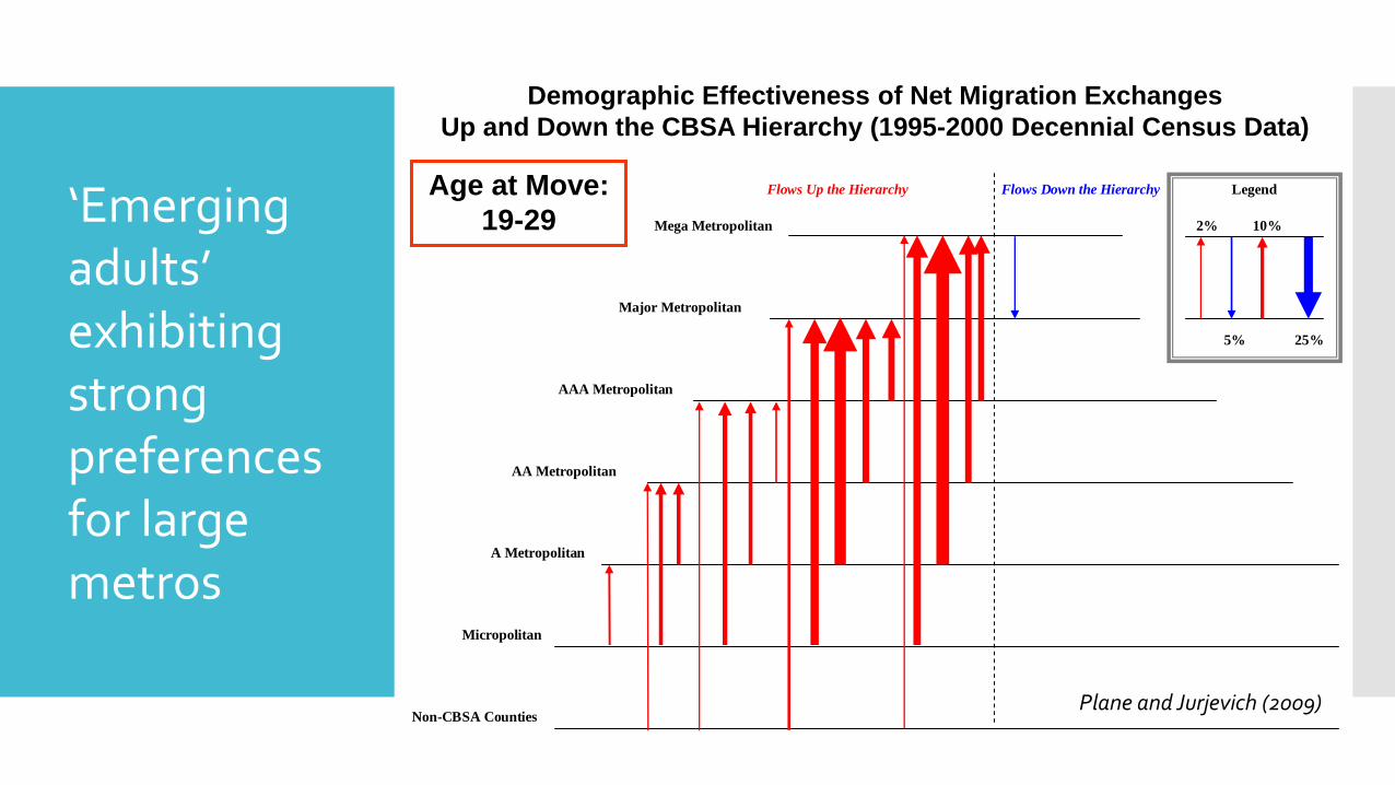
Demographic Effectiveness of Net Migration Exchanges

Up and Down the CBSA Hierarchy (1995-2000 Decennial Census Data)

Age at Move:

19-29‘Emerging adults’ exhibiting strong preferences for large metros

Plane and Jurjevich (2009)



Major Metropolitan

5% 25%

AAA Metropolitan

AA Metropolitan

A Metropolitan

Micropolitan

Non-CBSA Counties

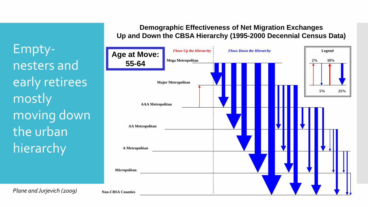
Demographic Effectiveness of Net Migration Exchanges

Up and Down the CBSA Hierarchy (1995-2000 Decennial Census Data)

Age at Move:

55-64

Empty-nesters and early retirees mostly moving down the urban hierarchy

Plane and Jurjevich (2009)



Major Metropolitan

5% 25%

AAA Metropolitan

AA Metropolitan

A Metropolitan

Micropolitan

Non-CBSA Counties



Major Metropolitan

5% 25%

AAA Metropolitan

AA Metropolitan

A Metropolitan

Micropolitan

Non-CBSA Counties



Major Metropolitan

5% 25%

AAA Metropolitan

AA Metropolitan

A Metropolitan

Micropolitan

Non-CBSA Counties



Major Metropolitan

5% 25%

AAA Metropolitan

AA Metropolitan

A Metropolitan

Micropolitan

Non-CBSA Counties

Demographic Effectiveness for Ages 80+


Major Metropolitan

5% 25%

AAA Metropolitan

AA Metropolitan

A Metropolitan

Micropolitan

Non-CBSA Counties



Major Metropolitan

5% 25%

AAA Metropolitan

AA Metropolitan

A Metropolitan

Micropolitan

Non-CBSA Counties

Age

15-24

Age

20-29

Age

25-34

Age

40-49

Age

55-64

Age

80+

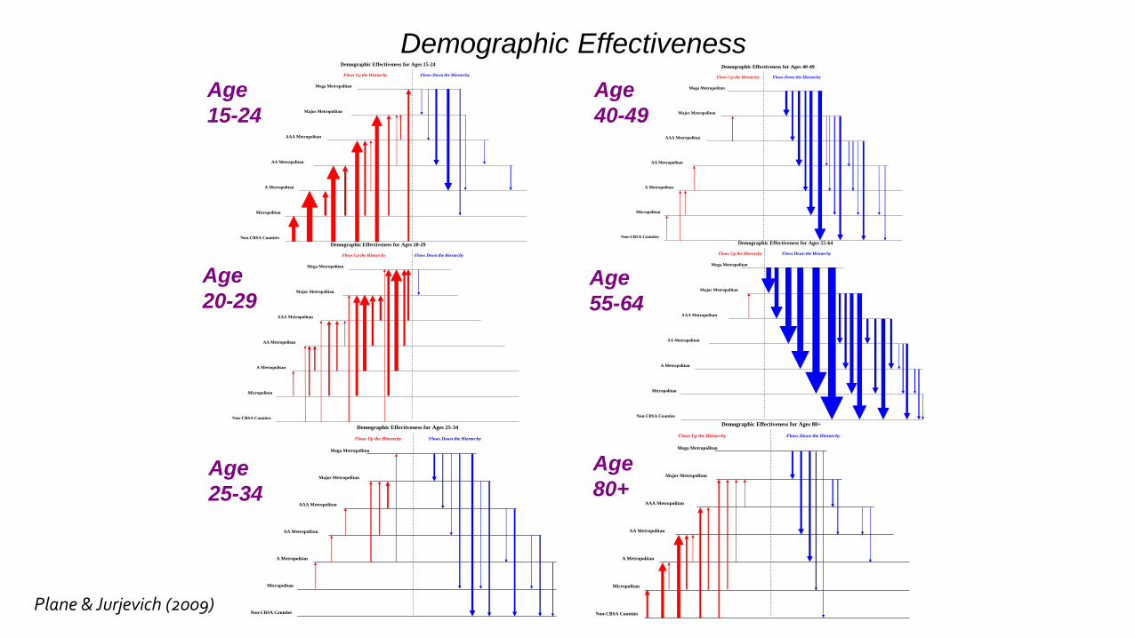
Demographic Effectiveness

Plane & Jurjevich (2009)

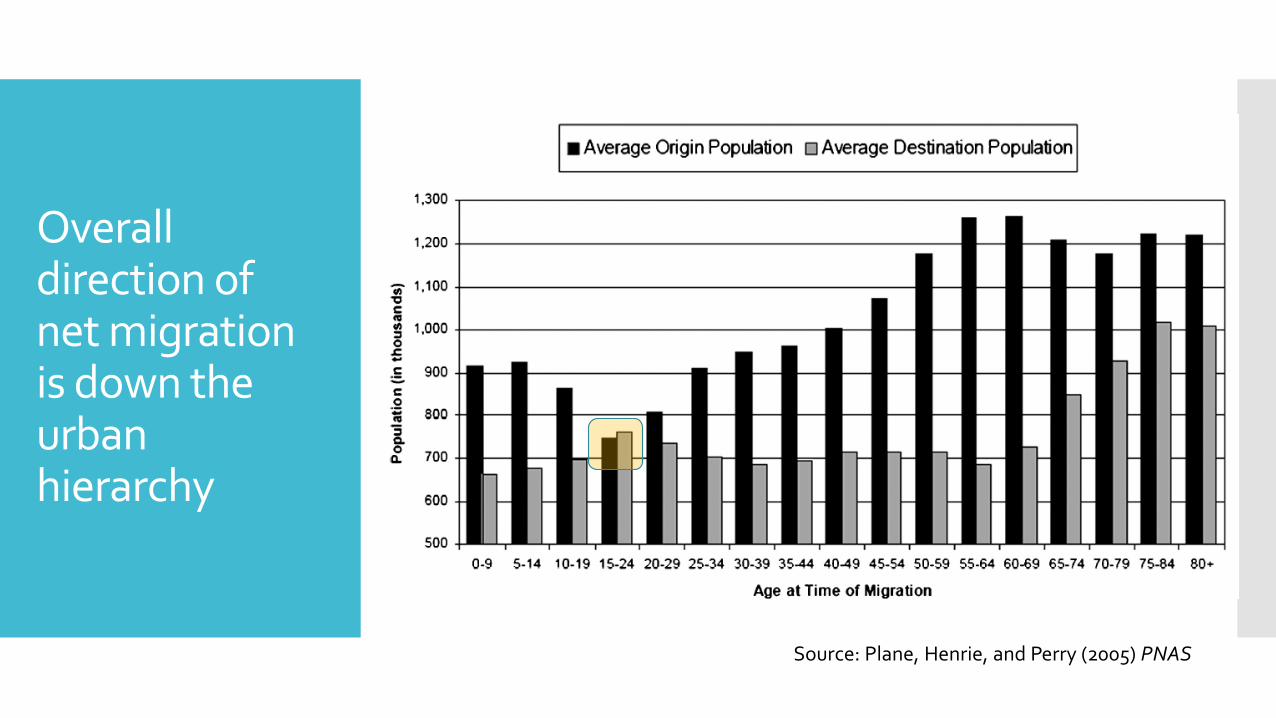
Overall direction of net migration is down the urban hierarchy

Source: Plane, Henrie, and Perry (2005) PNAS

Land use patterns at intra-metro scale of prime concern for climate change

2010 Census special report

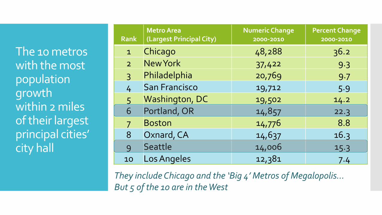
RankMetro Area(Largest Principal City)

Numeric Change2000-2010

Percent Change2000-2010

1 Chicago 48,288 36.22 New York 37,422 9.33 Philadelphia 20,769 9.74 San Francisco 19,712 5.95 Washington, DC 19,502 14.26 Portland, OR 14,857 22.37 Boston 14,776 8.88 Oxnard, CA 14,637 16.39 Seattle 14,006 15.3

10 Los Angeles 12,381 7.4

The 10 metros with the most population growth within 2 miles of their largest principal cities’ city hall

They include Chicago and the ‘Big 4’ Metros of Megalopolis…But 5 of the 10 are in the West

• Alan Ehrenhalt has trumpeted this downtown population revival as “The Great Inversion”

• Book is an interesting set of case studies of selected metros’ development trends—including Portland’s

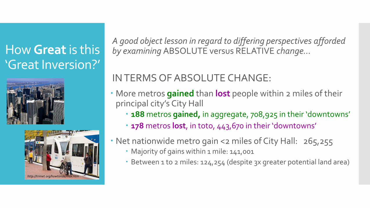
A good object lesson in regard to differing perspectives afforded by examining ABSOLUTE versus RELATIVE change…

IN TERMS OF ABSOLUTE CHANGE:

More metros gained than lost people within 2 miles of their principal city’s City Hall

188 metros gained, in aggregate, 708,925 in their ‘downtowns’

178 metros lost, in toto, 443,670 in their ‘downtowns’

Net nationwide metro gain <2 miles of City Hall: 265,255 Majority of gains within 1 mile: 141,001

Between 1 to 2 miles: 124,254 (despite 3x greater potential land area)

http://trimet.org/howtoride/max.htm

How Great is this ‘Great Inversion?’

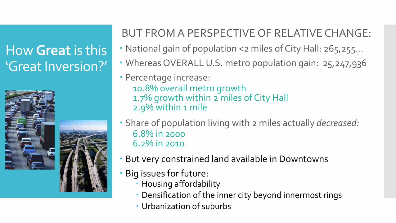
BUT FROM A PERSPECTIVE OF RELATIVE CHANGE:

National gain of population <2 miles of City Hall: 265,255…

Whereas OVERALL U.S. metro population gain: 25,247,936

Percentage increase:10.8% overall metro growth1.7% growth within 2 miles of City Hall2.9% within 1 mile

Share of population living with 2 miles actually decreased:6.8% in 20006.2% in 2010

But very constrained land available in Downtowns

Big issues for future: Housing affordability Densification of the inner city beyond innermost rings Urbanization of suburbs

How Great is this ‘Great Inversion?’

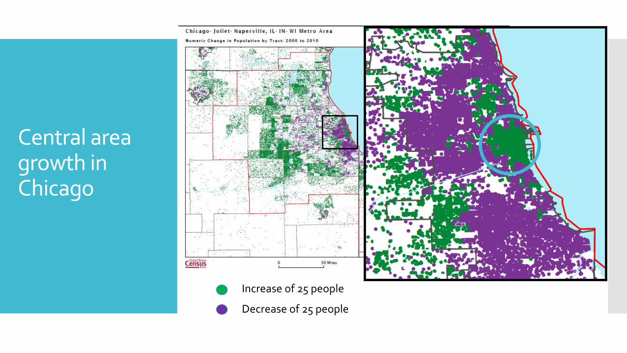
Central area growth in Chicago

Increase of 25 people

Decrease of 25 people

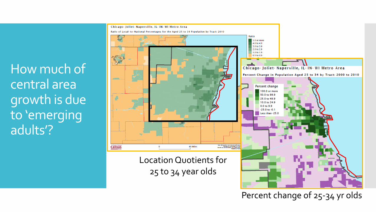
Location Quotients for 25 to 34 year olds

How much of central area growth is due to ‘emerging adults’?

Percent change of 25-34 yr olds

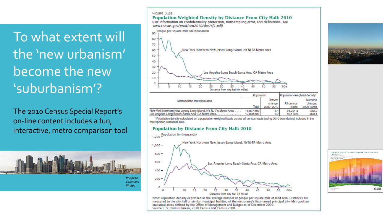
To what extent will the ‘new urbanism’ become the new ‘suburbanism’?

The 2010 Census Special Report’s on-line content includes a fun, interactive, metro comparison tool

Wikipedia Commons Photos

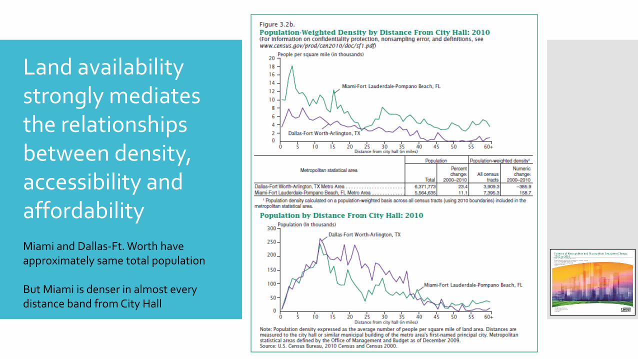
Land availability strongly mediates the relationships between density, accessibility and affordability

Miami and Dallas-Ft. Worth have approximately same total population

But Miami is denser in almost every distance band from City Hall

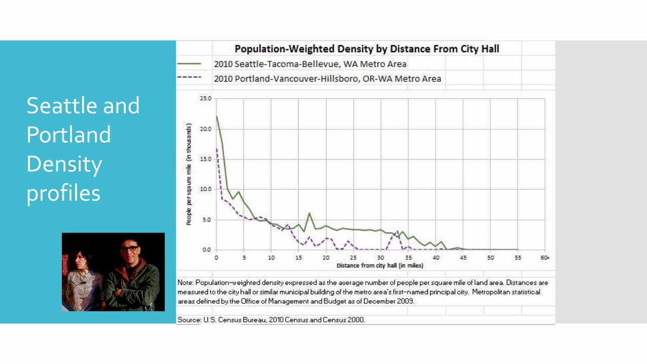
Seattle and Portland Density profiles

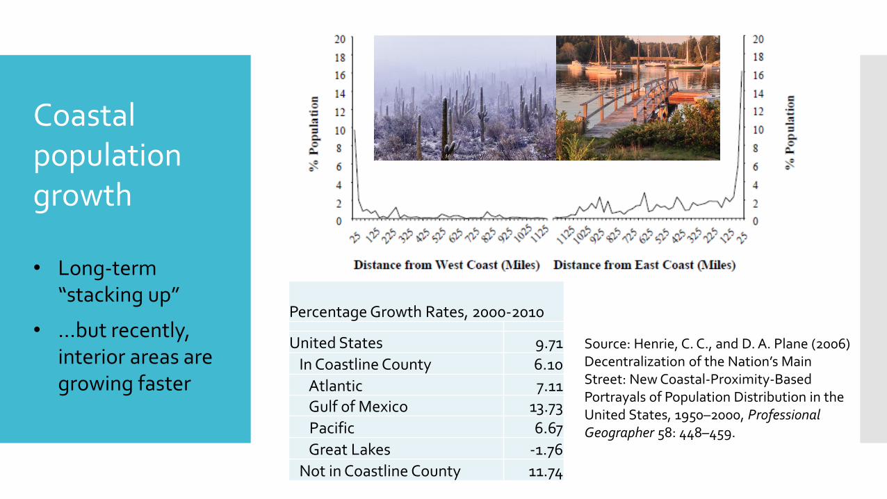
Source: Henrie, C. C., and D. A. Plane (2006) Decentralization of the Nation’s Main Street: New Coastal-Proximity-Based Portrayals of Population Distribution in the United States, 1950–2000, Professional Geographer 58: 448–459.

Percentage Growth Rates, 2000-2010

United States 9.71

In Coastline County 6.10

Atlantic 7.11Gulf of Mexico 13.73

Pacific 6.67

Great Lakes -1.76

Not in Coastline County 11.74

Coastal population growth

• Long-term “stacking up”

• …but recently, interior areas are growing faster

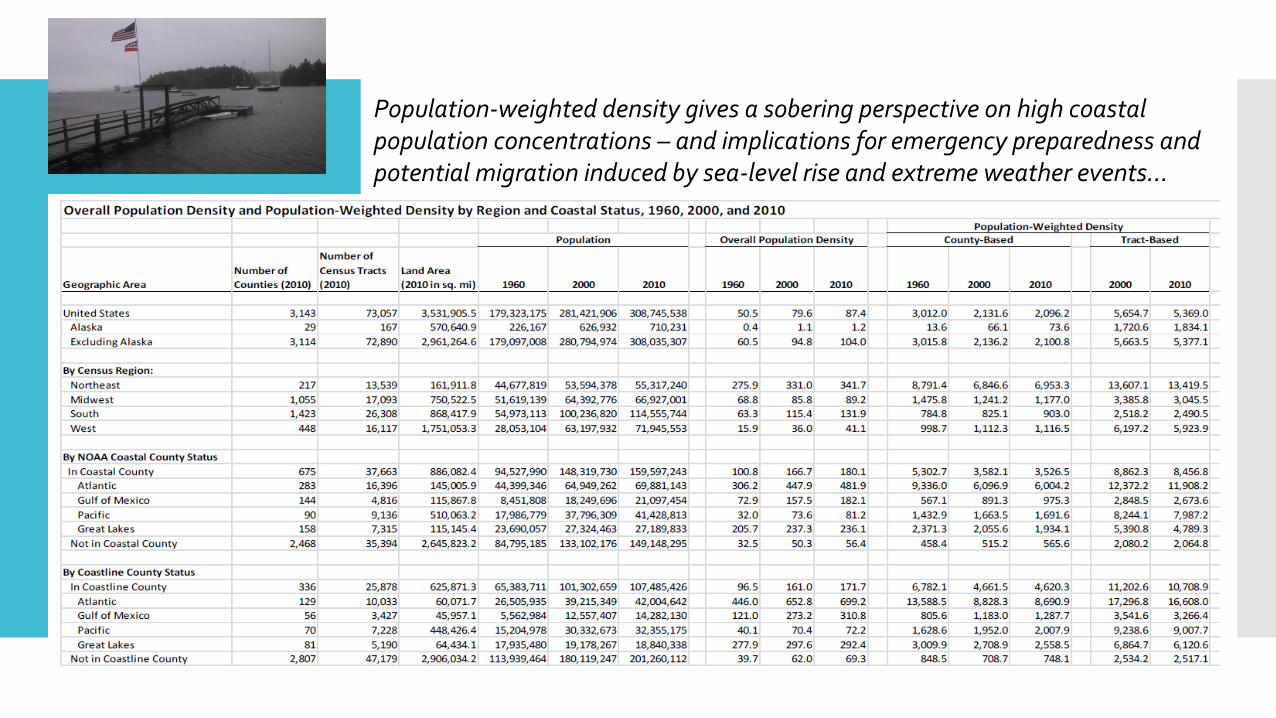
Population-weighted density gives a sobering perspective on high coastal population concentrations – and implications for emergency preparedness and potential migration induced by sea-level rise and extreme weather events…

ICLUS,Version 2

Integrated Climate and Land Use Scenarios

ICLUS,Version 2

Integrated Climate and Land Use Scenarios

EPA-based project to explores future changes in human population, housing density, and impervious surface for the United States

Projections broadly consistent with peer-reviewed storylines of population growth and economic development now widely used by the climate change impacts community

Two different climate models to illustrate the effect of changing climate variables on migration patterns :

First Institute of Oceanography-Earth System Model (FIO-ESM)

Hadley Global Environment Model 2 Atmosphere-Ocean (HadGEM2-AO)

Land use change projected down to 90 x 90 meter grid

The spatial allocation model incorporates National Land Use Dataset [US-NLUD] based on the 2011 National Land Cover Database

2000 to 2010 base period used to project out to 2100 Big inter-decadal variation in both climate and migration patterns

2000-2010 decade included ‘The Great Recession’

Aggregate migration data used, IRS county-to-county flows, so no linkage to age and age composition

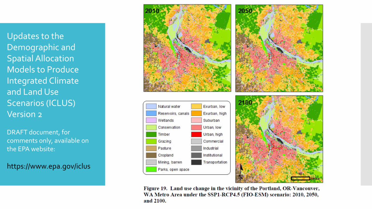
Updates to the Demographic and Spatial AllocationModels to Produce Integrated Climate and Land UseScenarios (ICLUS) Version 2

DRAFT document, for comments only, available on the EPA website:

https://www.epa.gov/iclus

Dave Plane

University of Arizona

[email protected]

Documents

Migration Patterns Today and the Factors that Influence Them