Embed Size (px)
Citation preview

1
Millionaire Migration in California: Administrative Data for Three Waves of Tax Reform
Charles Varner
Center on Poverty and Inequality, Stanford University
Cristobal Young
Center on Poverty and Inequality, Stanford University
Allen Prohofsky
Economics and Statistical Research Bureau, California Franchise Tax Board
Working paper: This is a work in progress, being circulated for input and feedback. Estimates
are preliminary and subject to revision. Please do not cite without permission
Keywords: millionaire taxes, fiscal policy, fiscal sociology, migration
Abstract
Does taxing the rich lead to migration of top income earners? In principle, barriers to migration
for the wealthy are low, suggesting that even small changes to top tax rates might set off tax
flight. Since top earners are also the largest taxpayers, the potential flight of the rich can set off a
race to the bottom, as states compete to attract (or retain) the rich with ever lower tax rates. We
draw on big administrative data covering 25 years of all top tax filers in California, showing
movement into and out of the state. We examine three waves of tax reform affecting top earners:
two “millionaire taxes” passed by voters via the proposition system in 2004 and 2012, and a tax
cut passed by legislation in 1996. We emphasize non-parametric, graphical analyses that reveal
the evidence with as few assumptions as possible and analogous regression models that confirm
the non-parametric results. Both in absolute terms, and compared to sensible control groups, we
find little migration response to changes in top tax rates.
We thank Chad Angaretis, Sean Lawrence, Teri Lovell, and Loi Quan of the California Franchise Tax Board
Economics and Statistical Research Bureau for their assistance and data expertise. Yue Li, Giovanni Righi, and
Ryan Leupp provided excellent research assistance. All findings are those of the authors, not positions of the
Franchise Tax Board, and the responsibility for any errors or omissions rests with the authors.

2
1 Introduction
A growing number of U.S. states have adopted “millionaire taxes” in recent years (Young
2017; Young and Varner 2011). These new tax brackets on the highest income earners offer a
way to address rising inequality while providing new revenues to support public goods and
services that can improve economic opportunity. The downside risk, however, is the concern of
millionaire tax flight – the richest residents may avoid the millionaire tax by moving to a
different state. While nine states have passed millionaire taxes, there are also nine states that
have no state income tax at all. How viable are millionaire taxes when lower-tax states are a
short distance away? Can states sustain these new millionaire taxes without suffering out-
migration of top tax payers? How attached are millionaires to the places where they currently
earn their income?
In the U.S. there are no formal borders that prevent individuals from moving across state
lines. Moreover, top income earners are often seen as highly mobile, and can easily bear the
fixed “moving truck” costs of migration (Feldstein and Wrobel, 1998; Sklair 2001). At the same
time, top earners are often late-career working professionals, and may be tied to place by the
immobility of their family and professional networks: their spouses, children, friends, colleagues,
investors, and clients may be reluctant to move for tax purposes (Young et al. 2016). Moreover,
agglomeration economies – such as the place-based centrality of Silicon Valley in the global
technology industry – are important considerations for state fiscal policy (Baldwin and Krugman
2004). Thus, a key question is whether – and by how much – top earners move away when states
enact a millionaire tax. Can states sustain these new revenue sources without losing their top tax
filers?
To address this question, we use big administrative data on all top earners in the state of
California, over 25 years. During this time period, California enacted two distinct millionaire
taxes (in 2004 and 2012), as well as a tax cut on top income earners (in 1996). We treat these as
a series of natural experiments in how sensitive millionaires are to changes in the ‘tax price’ of
living in California. We use difference-in-differences methods to see how a millionaire tax
affects those in the new tax bracket, compared to other high-income-earners who are just outside
the bracket. Roughly speaking, we examine tax changes affecting the top one percent, using the
95th to 99th percentiles as a control group.

3
This may seem like an exacting criteria, so we show each part of the analysis and offer
flexible sensitivity analyses at each stage.
1.1 The Fiscal Policy Tradeoff in Question
Millionaire taxes tend to be modest in magnitude, but can have significant impacts on
state budgets. In California, the 2004 Mental Health Services Tax (“2004 MHST”) raised the tax
rate on income above $1 million by one percentage point. Although just 0.3 percent of California
tax filers reported more than $1 million in the year it came into effect, these filers accounted for
more than 21 percent of all income in the state.1 Taxes on top earners have an outsized effect on
public revenues. At the same time, the migration of individuals in top tax brackets can have an
outsized negative impact on state finances.
For the wealthy, however, returns to human capital are one of several potential income
sources. In addition to wage and salary income, the wealthy may also draw on substantial capital
resources. To the extent that these resources are not tied to a particular place, some people at the
top of the income distribution may face fewer geographic constraints on earning capacity. If this
is the case, their residential decisions may depend more on the ‘tax price’ of a given jurisdiction.
However, the presumption that exceptionally skilled, monied, and entrepreneurial
individuals are also exceptionally mobile is debatable. Certainly, some millionaires do have the
luxury of greater mobility, and recent studies verify Mirrlees’ (1982) proposition in specific
cases. For example, Kleven, Landais, and Saez (2013) show that European football stars prefer to
play for teams in countries with lower tax rates. Yet, as the authors note, professional sport
requires minimal place-specific investment of human capital. In fact, the game itself moves
around, often across international borders. Kleven et al. (2013) provide an important upper
bound estimate on the migration responsiveness of the highly skilled. Nevertheless, their
estimated tax-elasticity of residential location is still only 0.4, suggesting that place
considerations are significant even for the most mobile top earners.
Wealthy tax filers may also be quite immobile. Positions in the most highly-skilled and
most highly-remunerated professions are concentrated in particular places. Consider
technological expertise in Silicon Valley or financial expertise on Wall Street. The
agglomeration economies in these regions are important considerations for state fiscal policy
1 Source: Franchise Tax Board, 2006 Annual Report, p. 82.

4
(Baldwin and Krugman 2004). To be sure, there are top-income earners who do not depend on
labor income. Yet even members of this group will have invested significant economic and
social resources in a particular place in order to make their fortunes (Glaeser and Gottlieb 2009).
But taxes may be consequential for wealthy households. In absolute terms, the wealthy
pay more taxes. They may also be able to “time” income and more easily withstand any
interruption of earnings associated with an interstate move. Indeed, the potential tax effect on
migration is at the center of a largely separate literature on regional tax competition. In short, the
threat of greater migration responsiveness among the wealthy suggests a policy tradeoff between
the “millionaire taxes” that are often popular with voters, and the loss of wealthy tax filers. If
millionaires are in fact more mobile, state policymakers may be forced to “curse” the less-mobile
middle with the largest tax bills (Simula and Trannoy 2011).
Young and Varner (2011) examined the migration response to a millionaire tax in New
Jersey, which raised its income tax rate on top-income earners by 2.6 percentage points. In many
ways New Jersey was an ideal testing ground, given its close proximity to lower-tax states
(Connecticut and Pennsylvania) with whom New Jersey shares two multi-state cities (New York
and Philadelphia metropolitan areas). The geography of New Jersey makes it relatively easy to
arbitrage state tax systems without leaving one’s city.
Drawing on the complete New Jersey state tax micro data (a virtual census of
millionaires), that study found little responsiveness to the tax increase, with semi-elasticities
generally below 0.1. There was evidence of modest tax-induced migration among some small
segments of the millionaire population: millionaires past retirement age and those living
primarily on investment income rather than wages (i.e., people not tied to their state by an
employer or business). Overall, the New Jersey tax raises roughly $1 billion per year and
modestly reduces income inequality. This research was later replicated by Cohen, Lai, and
Steindel (2015) who were critical but reported new estimates that were largely within the
confidence intervals of the original study (Young and Varner 2015).
More recent work on elite populations comes from Akcigit et al. (2016) and Moretti and
Wilson (2017) studying star scientists internationally and in the U.S. These studies show a range
of estimates. Akcigit et al. (2016) use similar methods to Kleven et al. (2013) and find large
effects for foreign-born elites, but small effects for those living in their country of birth. It should
be noted that in both studies, only a very small fraction of their samples are foreign-born (around

5
five percent). Moretti and Wilson (2017) find larger effects of tax changes on star scientists
within the U.S., and conclude that taxes on the rich are one important factor driving location
choices of elite scientists and perhaps “other well-educated, productive, and high-income
workers” (1861).
1.2 California Income Tax Rates
In California, the personal income tax rate structure has changed many times since its
introduction in 1935. From the beginning, California had a progressive rate structure. In the early
years, the income tax started at 1 percent on income below $5,000, rising to a 15 percent top
marginal rate on income above $250,000 (not adjusted for inflation).
Since 1935, the top marginal rate has changed 9 times, with 6 increases and 3 cuts.
Figure 1.1 places these changes in economic context. It shows the top marginal tax rate against
the backdrop of the business cycle, with recessions indicated by the shaded columns. The top tax
rate has ranged between 6 percent and 15 percent. After a very large tax cut in 1942, the long-
term trend has been towards higher top tax rates in the state. Since 1973, the top rate has
fluctuated between 9.3 percent and 13.3 percent – and this is the magnitude of policy difference
we observe in our current data.
It is worth noting that, compared to states like Nevada, Texas, or Florida, California has
had high taxes on the rich for some eight decades. Relatively high taxes on top income in
California are older than Silicon Valley, the modern computer, or the Golden Gate Bridge. When
taxes on high income earners were first established in California, movies with sound were called
“talkies” and the famous LA sign read “Hollywoodland.” We do not know how California’s
socio-economic history might have unfolded differently if, like Texas, it never had an income
tax.
Over the last 25 years, tax rates on top incomes in California have gone up and down
within a range of four percentage points. Our empirical question is limited to asking: does it
matter whether a state’s top tax rate is 9.3 or 13.3 percent? If a state raises its top tax rate on this
type of scale, would top income earners leave the state?
This is a question that generates very heated policy debates. In California, top Republican
lawmakers argued that “nothing is more portable than a millionaire and his money” (Yamamura

6
2011). In Oregon, Phil Knight – the CEO of Nike and the state’s richest resident – warned that a
millionaire tax would “set off a death spiral” of top earners fleeing the state (Knight 2010).
Figure 1.1 California top marginal tax rate, 1935–present
Note: Recession years shaded in grey. Source: California Franchise Tax Board.
In this paper, we analyze three specific episodes of tax reform. First, we focus on two
“millionaire taxes” passed in 2004 and 2012, respectively. These reforms introduced new tax
brackets and higher rates for high income earners.
Figure 1.2 (below) shows the rate schedule before and after the 2004 Mental Health
Services Tax came into effect. In November 2004, voters approved Proposition 63, which added
1 percentage point on income above $1 million effective January 1, 2005. Before this, marginal
rates were progressive at low and middle income levels, but topped out at about $40,000 for
single filers or $80,000 for joint filers. Between 1996 and 2004, the marginal rate was the same
(9.3 percent) for the top one-fifth of all income earners. Since the 2004 increase, income earners
at the very top paid 10.3 percent on income above $1 million.
0%
2%
4%
6%
8%
10%
12%
14%
16%
1935 1940 1945 1950 1955 1960 1965 1970 1975 1980 1985 1990 1995 2000 2005 2010 2015
Year
Marginal tax rate
1991-1995:11.0%
Marginal tax rateMarginal tax rate
1996-2004:9.3%
1935-1942:15.0%
1943-1958:6.0%
1973-1986:11.0%
1987-1990:9.3%
2012+:13.3%

7
Figure 1.2 The 2004 Mental Health Services Tax
In 2012, voters approved a larger set of tax increases on high income earners, starting at
$250,000 for single filers and $500,000 for married couples. Proposition 30 added three new tax
brackets, as shown in Figure 1.3. It is worth noting that the Proposition 30 tax schedule was
originally set to expire in 2019, but was re-approved by voters under Proposition 55 in 2016 to
extend to the year 2030.

8
Figure 1.3 The 2012 (Proposition 30) Tax Increases
Note: Brackets shown are for single filers. Bracket cut points were doubled for joint filers.
Figure 1.4 (below) provides a similar picture for the 1996 tax cuts, which returned the top
marginal rate to its 1990 level. One important difference is that the 1996 changes applied to a
much wider income range. The 1996 changes were not “middle class tax cuts,” but any single
filer above $109,936 or joint filer above $219,872 received a tax cut of up to 1.7 percentage
points.

9
Figure 1.4 The 1996 Tax Cuts
Note: Brackets shown are for single filers. Bracket cut points were doubled for joint filers.
1.3 California’s Wealthy Population
Have tax policy reforms altered California’s ability to cultivate, attract, or retain the
wealthy? If tax rates are important factors in the state residency decisions, we would expect to
find two patterns in California’s wealthy population. The number of top income earners would
fall after a tax increase and rise after a tax cut.
Figure 1.5 (below) shows the number of millionaires in the California tax data since
1990. The millionaire population grew from 15,000 in 1990 to more than 150,000 in 2007, and
nearly 200,000 in 2014.2 None of the tax changes we study has a visually-perceptible effect on
the general upward trend in the number of millionaires filing taxes in California. After the 2004
MHST came into effect, the number of millionaires continued to rise for three years, falling only
during the 2008 financial crisis. This pattern does not indicate that the recent tax changes were of
major concern to top-income earners.
If the population of top earners were determined mostly by tax rates, the basic population
graph could be quite informative. However, population changes for other reasons. The strength
2 These counts include all California residents and nonresidents who had income greater than $1 million.

10
0
50,000
100,000
150,000
200,000
1990 1992 1994 1996 1998 2000 2002 2004 2006 2008 2010 2012 2014
Number of Millionaires Filing Tax Returns, 1990-2014
1996 tax cuts2005 tax increase
2012 tax increase
of financial markets is critical, with the two peaks in Figure 1.5 corresponding to the dot-com
boom (1999-2000) and the more recent stock market run-up (2007-08). These economic trends
greatly increased the number of Californians earning very high incomes. Analytically, other
drivers of the top-income population (particularly income growth) overshadow migration, which
occurs on a smaller scale.
Figure 1.5 Number of Millionaires Filing California Tax Returns, 1990–2014
Source: FTB microdata.
In the results that follow in this paper, we interpret migration effects relative to the base
population of millionaires. Yet, as Figure 1.5 makes clear, the size of that population changes
dramatically over the business cycle.
Thus, though the net migration and millionaire population trends indicate that the tax
changes had no effect on California’s attractiveness to the wealthy, we need to examine
migration data for top-income earners in order to identify any potential tax effect on migration.
It is this analysis to which we turn now. The rest of the paper has four sections. Section 2 defines

11
migration events in the FTB data and illustrates the intuition guiding our difference-in-
differences models. Section 3 presents our main non-parametric graphical analysis of the 2004
Mental Health Services tax, the 2012 Proposition 30 tax, as well as basic results for the 1996 tax
cut. In Section 4, we estimate regression models for the two millionaire taxes and conduct a
sensitivity analysis of the average effect across top earner socio-demographic groups. Section 5
provides extensions and robustness tests. Section 6 concludes.
2 Data and Identification Strategy
Administrative tax data have unique value for the study of top-income migration
behavior. For this study, the California Franchise Tax Board (FTB) granted us access to a
longitudinal panel of de-identified tax records. Using data from California personal income tax
returns, the FTB created data sets for the tax years 1990-2014. Resident tax returns (Forms 540,
540A, 540EZ, and 5402EZ) and part-year / non-resident tax returns (Forms 540NR Long and
540NR Short) were included.
FTB then conducted three data processing steps necessary for the creation of a reliable
longitudinal data set. First, because it is possible to file a tax return for a tax year other than the
filing year, it was necessary to transfer the information from these returns to the appropriate tax
year. Second, for each tax year, data on joint filers was replicated. The designation of the
primary and secondary filers was switched on the replicated record. Third, the replicated tax year
datasets were merged to create a panel dataset. This method creates an observation with time
series data for each adult taxpayer regardless of changes in marital or filing status. After
perfecting the data set, FTB removed identifying information such as names and SSNs from the
data file to preserve taxpayer confidentiality.
The data set we received from FTB provides a virtual census of high-income earners,
with information on income, taxes paid, and some limited demographic data reported on a
standard tax form (such as marital status). Our analysis of the 2004 Mental Health Services tax
includes the filing history for any filer who reported annual adjusted gross income above
$500,000 at least once in the FTB data. There are an average of 750,000 records per year, giving
roughly 13.5 million records in total for the 2004 MHST analysis.

12
2.1 Migration Definitions
In this section, we discuss how migration is defined using the FTB data. Individuals in
the tax data can have one of three basic filing statuses in any given year:
F = Full-year resident tax return
P = Part-year / non-resident tax return
M = Missing (no tax return)
We add subscripts to the notation to indicate the year relative to the reference year. So, if the
reference year is 2004, then subscript -1 means 2003, 0 means 2004, and +1 means 2005.
In-Migration
Three year definition: MPF = M-1P0F+1
This definition of in-migration refers to the following sequence of tax filing: no tax return
filed (M-1), then a part-year return in the reference year (P0), then a full-year return (F+1).
Though these individuals file their first full-year resident return in year +1, they arrived in
California in the reference year 0.
Out-Migration
Three year definition: FPM = F-1P0M+1
This is the opposite sequence from in-migration: beginning with a full-year resident
return (F-1). In the reference year a part-year return is filed (P0), followed by no tax return filed
in the following year (M+1). These tax filers are coded as leaving the state when they filed their
part-year tax return, which is reference year 0.3
Net Migration
We define net migration as the difference of in-migration minus out-migration, or MPF –
FPM. Net migration gives the overall change in the millionaire population due to migration
flows.
3 In Appendix B, we discuss using alternative four-year migration definitions, such as F-1P0M+1 M+2 to define out-
migration, and robustness tests are available on request.

13
2.2 Basic Facts on Millionaire Migration
As a baseline descriptive analysis, we examine the trends in net migration to California
for taxpayers with annual incomes of $1 million or more, i.e. those whose income would be
exposed to both the 2004 and 2012 tax increases. Figure 2.1 shows net migration rates from 2001
through 2014.4 It is clear that there is not a pattern of millionaire out-migration in recent years
despite the 4 percentage point tax increase on income above $1 million since 2004 (rising from a
rate of 9.3% to 13.3% in 2012). If anything, the trend has run counter to the tax-flight
expectation. There was a small net outflow of millionaires leaving California in the years prior to
the first tax increase, but this outflow decreased in 2005 and 2006, and then shifted to a positive
inflow of millionaires to California in 2007. This net migration of millionaires into the state has
remained positive since 2007 even in the years since the much larger 2012 tax increase, though
the inflow rate slowed somewhat in 2013 and 2014.
Figure 2.1 Millionaire Net Migration to California, 2001-2014
Note: Estimates show net migration as a percent of the base millionaire population.
In this first look at the data, we do not compare millionaires’ migration rates to the rates
of a control group. We will do that in a moment. However, it is worth emphasizing that, on net,
millionaires have been moving into California at a greater pace after two tax reforms that
increased the state’s tax price. We also reiterate here, before turning to our main difference-in-
4 Net migration is defined as (in-migrants – out-migrants) / base population.
-0.30%
-0.20%
-0.10%
0.00%
0.10%
0.20%
0.30%
0.40%
2001 2003 2005 2007 2009 2011 2013
2004 tax reform
2012 tax reform

14
differences models, that migration comprises a very small portion the year-to-year change in
millionaire population. Appendix Table A.1 shows the raw counts of base population, in-
migrants, and out-migrants in each year, for millionaires and for similar high-income earners
between $500,000 and $1 million. One can see that the net migration counts (in particular) are
very small relative to the base population.
The population of full-year resident millionaires has ranged from about 42,000 to 93,000,
while out-migration has ranged from about 300 to about almost 600. Net migration has ranged
from -116 to 150. One standard deviation in the population of millionaires is 18,750; the
corresponding number for net migration is 85. Migration accounts for less than one-half of one
percent of the variation in the number of millionaires in California.
To make this point more intuitively clear, Table 2.1 shows the annual change in the
population of California millionaires, along with the annual change in the net migration of
millionaires, before and after the 2004 MHST. The number of millionaires has gone up or down,
on average, by 11,772 people a year. The net migration of millionaires has gone up or down by
59 people.5 Migration accounts for just one-half of one percent (0.5%) of the changes in the
millionaire population.
Table 2.1 Millionaire Population Changes
Change in
Number of
Millionaires
Change in Net
Migration of
Millionaires
2002 -7,663 26
2003 6,671 -12
2004 15,419 -86
2005 13,280 93
2006 8,625 -11
2007 7,680 135
2008 -23,067 49
Average of
Absolute
Changes 11,772 59
5 Absolute changes ignore the signs (i.e., whether the population change was positive or negative) and focuses
simply on the magnitude of typical year-to-year changes.

15
Some 99.5 percent of fluctuation in the size of the millionaire population is driven by something
other than migration – mostly, income dynamics at the top – California residents growing into
the millionaire bracket, or falling out of it again.
Despite the limited importance migration plays for the size of California’s millionaire
population, the central goal of the paper is to identify the responsiveness of migration to top tax
rates.
2.3 Identification Strategy
How does one identify the effect of a millionaire’s tax on migration? We use two
complementary strategies. First, we look simply at annual migration rates for treatment and
control groups. The treatment group is composed of individuals who earn enough to place them
inside the tax bracket – i.e., people who pay more under the new tax rate. For the 2004 MHS tax,
the treatment group is individuals who earned more than $1 million in a year after 2004. The
control group is composed of high-income individuals who are not subject to the tax increase.
We define the control group to be those earning $500,000 to $1 million in a year.
There may well be differences in the migration rates between the treatment and control
group. This is acceptable, since we are looking for a divergence between these groups’ migration
rates that occurs after the tax was introduced. Thus, we do not require that the treatment and
control groups have the same baseline migration rates. We simply expect that the tax creates a
new difference between the groups after 2004. Specifically, the net migration rate should
increase for those affected by the tax relative to those in the control group.
The principal purpose of the control group is to capture (non-tax) social, political, and
macroeconomic trends that affect the migration behavior of top-income earners. The effect of the
tax is observed by a new decrease in net migration (in-out) among the treatment group, but not
among the control group.
Our first strategy models the tax increase as if it were a lump sum fee that falls equally on
all individuals with more than $1 million in income. However, with a marginal tax rate, all
income up to $1 million is exempt from the higher rate. The new rate only applies to earnings
above $1 million. Thus, for individuals earning $1,000,001, their tax increase is 1 penny. For
those making $10,000,000, their tax increase is $90,000. Thus, the magnitude and the effective
rate of the tax increase grows with the amount earned above $1 million. Our second

16
identification strategy takes this into account. Thus, we not only expect a net migration response
for the treatment group relative to controls. We also expect that any effect of the tax change
would increase as income increases within the treatment group.
If the tax were to have an effect on out-migration, Figure 2.2 illustrates the change we
would expect, by detailed income levels. (Using real data, we break up the control and treatment
groups into income deciles; the income levels depicted here reflect our income deciles.) The
solid line shows the income-migration profile for the pre-tax years, depicted here as completely
flat: as income grows, out-migration rates remain constant. The dashed line shows the expected
income-migration profile after the tax increase. On the left-hand side of the graph, we see that
migration rates were unaffected for those earning less than $1 million. The right-hand-side shows
a steadily increasing out-migration rate. This reflects the fact that those in the treatment group
with the highest incomes experienced the largest tax increases – both in dollar terms, and in their
effective tax rate.
Figure 2.2 Expected Effect on Out-migration Rates after the 2004 MHST
17
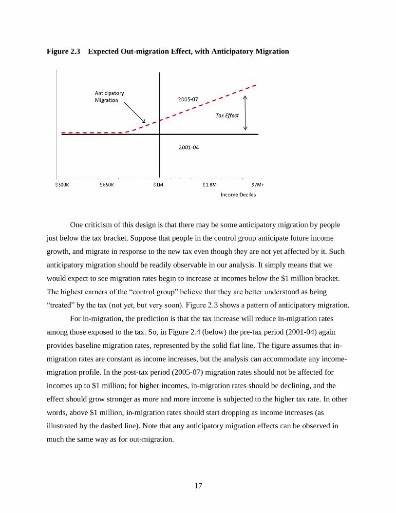
Figure 2.3 Expected Out-migration Effect, with Anticipatory Migration
One criticism of this design is that there may be some anticipatory migration by people
just below the tax bracket. Suppose that people in the control group anticipate future income
growth, and migrate in response to the new tax even though they are not yet affected by it. Such
anticipatory migration should be readily observable in our analysis. It simply means that we
would expect to see migration rates begin to increase at incomes below the $1 million bracket.
The highest earners of the “control group” believe that they are better understood as being
“treated” by the tax (not yet, but very soon). Figure 2.3 shows a pattern of anticipatory migration.
For in-migration, the prediction is that the tax increase will reduce in-migration rates
among those exposed to the tax. So, in Figure 2.4 (below) the pre-tax period (2001-04) again
provides baseline migration rates, represented by the solid flat line. The figure assumes that in-
migration rates are constant as income increases, but the analysis can accommodate any income-
migration profile. In the post-tax period (2005-07) migration rates should not be affected for
incomes up to $1 million; for higher incomes, in-migration rates should be declining, and the
effect should grow stronger as more and more income is subjected to the higher tax rate. In other
words, above $1 million, in-migration rates should start dropping as income increases (as
illustrated by the dashed line). Note that any anticipatory migration effects can be observed in
much the same way as for out-migration.

18
Figure 2.4 Expected Effect on In-migration Rates, after the 2004 MHST
The 2012 (Prop 30) tax reform was more complex than the 2004 MHST, as it involved several
new brackets, which also depended on filing status (e.g., higher brackets for those married filing
jointly than for single individuals). However, the basic form of the identification strategy is
similar: there is a control group of high-earners not affected (below the new brackets), and a
treatment group for whom the tax bite rises with income above the new bracket. Thus, we will be
similarly looking for a tax effect that grows in magnitude as income rises in the treatment group.
3 Graphical Analysis
In this section, we describe the graphical analysis of millionaire migration in the wake of
tax increases on top income earners. This provides a purely non-parametric analysis.
Specifically, this shows the average migration rates by deciles of top income earners for
treatment and control groups, both before and after the three tax reforms we consider. First, we
examine the 2004 Mental Health Services Tax. Then, we apply a similar analysis to the 2012
(Proposition 30) tax increase and the 1996 tax decrease.
3.1 The 2004 Mental Health Services Tax
We begin simply, looking at migration rates by detailed income group before and after
the 2004 tax reform. On the left-side of Figure 3.1, we show the control group ($500,000 to $1

19
million) divided into ten income deciles. The solid line shows out-migration rates at each control
group decile’s income in period 1 (before the millionaire tax passed), while the dashed line
shows out-migration rates in period 2, after the tax was passed. For those with incomes up to $1
million, who were not affected by the tax change, there is no shift in out-migration rates. Overall,
out-migration among the control group was 0.9 percent in both periods. The right-side of Figure
3.1 shows out-migration rates by deciles of treatment group income. In both periods, out-
migration rates decline with income, indicating that the highest earners are more attached to the
state. Moreover, out-migration rates are notably lower in period 2, after the millionaire tax had
passed. This is a wrong-signed effect. The tax flight argument anticipates increasing out-
migration among the highest earners ($1 million+) after a tax increase. However, after the 2004
MHST, we observe the opposite. For the treatment group, out-migration falls from 0.8% to 0.6%.
The difference-in-differences estimate is calculated as the decline for the treatment group minus
the constant trend for the control group (which provides the counter-factual expected migration
patterns had the MHST not come into effect). The DiD estimate is -0.2 percent.
Figure 3.1 Out-migration Rates by Income, before and after the 2004 MHST
0.0%
0.2%
0.4%
0.6%
0.8%
1.0%
1.2%
$500K $650K $1M $1.8M $7M+
Period 1
Period 2
Treatment group ($1M+) deciles
Out-migration rate
Control group ($500k - $1M) deciles

20
Before After Diff
Control 0.9% 0.9% 0.0% Treatment 0.8% 0.6% -0.2%
Diff -0.1% -0.3% -0.2%
Figure 3.2 turns the focus to in-migration from other states. It follows the general pattern
of decline with income: high-income individuals are less likely to be new in-migrants. However,
the pattern is the same both before and after the 2004 MHST. Support for the tax flight argument
would require declining in-migration among those exposed to the tax after it was passed. The
simple DiD estimate is zero.6
Figure 3.2 In-migration Rates by Income, before and after the 2004 MHST
Before After Diff
Control 0.9% 0.9% 0.0% Treatment 0.7% 0.7% 0.0%
Diff -0.2% -0.2% 0.0%
6 Appendix Table A.2 shows the decile cut points for both the control and treatment groups, and shows the
in- and out-migration rates at each level (as plotted in Figures 3.1 and 3.2).
0.0%
0.2%
0.4%
0.6%
0.8%
1.0%
1.2%
$500K $650K $1M $1.8M $7M+
Period 1
Period 2
Income Deciles
In-migration rate

21
Finally, Figure 3.3 plots net in-migration rates (in-migration minus out-migration, divided by
population). Overall, net-migration of top earners over this period was close to zero: out-
migrations are evenly matched by in-migrations at each income level. However, Figure 3.3 also
shows net in-migration rising slightly in period 2, after the millionaire tax had taken effect.
Clearly, the effect size is small, but wrong-signed: net in-migration of millionaires rose after the
tax was passed, by an amount equal to 0.2 percent of the base millionaire population. As noted
above, this pattern is driven entirely by declining out-migration of millionaires in period 2;
patterns of in-migration did not change.
Figure 3.3 Net In-migration by Income, before and after the 2004 MHST
Before After Diff
Control 0.0% -0.1% 0.0% Treatment -0.1% 0.1% 0.2%
Diff -0.1% 0.1% 0.2%
This analysis shows that in the years after the tax took effect, net migration for the
treatment group (those exposed to the tax) increased relative to migration rates for the control
group. The magnitude of difference is very small. Nonetheless, net migration of millionaires
turned positive, while net migration of half-millionaires turned negative in the years after the tax.
-0.6%
-0.4%
-0.2%
0.0%
0.2%
0.4%
0.6%
$500K $650K $1M $1.8M $7M+
Period 1
Period 2
Income Deciles
Net In-migration rate (in minus out)

22
A reasonable interpretation is that, for both groups, net migration was “zero-plus-noise” over the
whole period. But from an accounting perspective, there was a gain in millionaires after the tax.
3.2 The 2012 (Proposition 30) Tax Increase
In 2012, California voters approved Proposition 30, which raised taxes on top incomes by
upwards of three percentage points.7 Specifically, the tax provided new brackets starting at
$250,000 (10.3%), $300,000 (11.3%), $500,000 (12.3%) and retained the additional 1 percent
marginal tax above $1 million (13.3%).8 The proposition passed in November, 2012, but applied
retroactively to income earned since January of that year. Thus, we treat 2013 as the first year
top earners could behaviorally respond to the new tax rates.
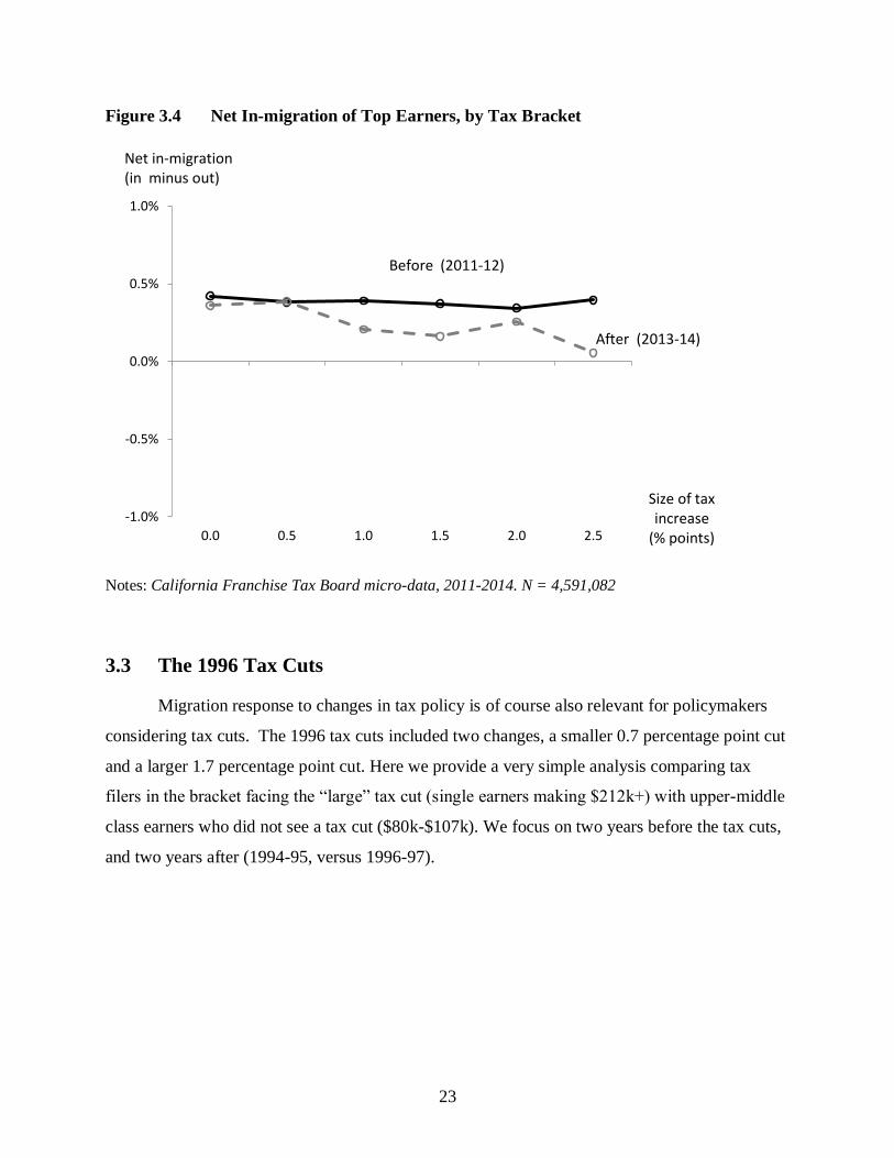
Figure 3.4 (below) shows net in-migration of millionaires before and after the 2012 tax
increase, by tax bracket (i.e., percentage point tax increase). For this analysis, we grouped tax
filers by the effective tax increase they experienced (defined by income and filing status), and
calculated net in-migration for those groups before and after the passage of Proposition 30.
The leftmost points in Figure 3.4 represent the control group – high income earners who
were just below the cut point for any tax increase. Moving rightward along the graph shows
groups that saw increasingly larger effective tax increases. The rightmost observations show
people who saw a 2.5 to 3 percentage point effective tax increase. Net in-migration was positive
and roughly constant across these income brackets in the two years before the tax increase
(2011-12). However, after 2012, net in-migration declines for those facing an effective tax
increase of 0.5 percentage points or higher. The net-migration decline is largest for the group
facing the highest effective tax increase. Overall, this is consistent with a tax flight response that
is roughly linear in the magnitude of the tax increase (albeit with noise).
On average, the difference-in-difference estimates from Figure 3.4 give a semi-elasticity
of -0.04 percent, meaning a loss equal to 0.04 percent of the millionaire population, or roughly
one-twenty-fifth of one percent, for a percentage point increase in the effective top tax rate.
7 Proposition 30 passed by a margin of 55 percent in favor, 45 percent opposed. 8 These are the new brackets for single and separate filers. The new brackets for married and widowed filers started
at twice these income levels. For heads of households, the new brackets began at $340,000 (10.3%), $408,000
(11.3%), and $680,000 (12.3%). These income levels have been adjusted upwards each year since 2012 for inflation.
23
Figure 3.4 Net In-migration of Top Earners, by Tax Bracket
Notes: California Franchise Tax Board micro-data, 2011-2014. N = 4,591,082
3.3 The 1996 Tax Cuts
Migration response to changes in tax policy is of course also relevant for policymakers
considering tax cuts. The 1996 tax cuts included two changes, a smaller 0.7 percentage point cut
and a larger 1.7 percentage point cut. Here we provide a very simple analysis comparing tax
filers in the bracket facing the “large” tax cut (single earners making $212k+) with upper-middle
class earners who did not see a tax cut ($80k-$107k). We focus on two years before the tax cuts,
and two years after (1994-95, versus 1996-97).
-1.0%
-0.5%
0.0%
0.5%
1.0%
0.0 0.5 1.0 1.5 2.0 2.5
Net in-migration(in minus out)
Size of tax increase
(% points)
Before (2011-12)
After (2013-14)

24
Figure 3.5 Net In-migration Rates, 1994-97
Source: FTB Microdata. N = 9,048,672
Net migration was trending positive for all groups during this period, as shown in Figure
3.5. These were economic boom times for California. Net out-migration of the early 1990s was
turning towards net in-migration in the late 1990s. However, what is most striking about Figure
3.5 is the parallel trend between the top earners enjoying a “large” tax cut, and the control from
of upper-middle earners that received no tax break at all. For the tax flight hypothesis, the “large
tax cut” group should have a growing divergence from the controls after 1995. These results give
no evidence of a migration effect of the 1996 tax cut.
This is a preliminary analysis of the 1996 tax cuts, and in the next version of this paper
we will present more detailed analysis. For now, Appendix C provides table summaries of the
control and treatment groups, including their population and migration data, as well as basic
difference-in-difference estimates of tax migration.
-1.0%
-0.6%
-0.2%
0.2%
0.6%
1.0%
1994 1995 1996 1997
1996 tax cut
No tax cut group
Large tax cut group

25
4 Regression Analysis
In this section, we estimate analogous regression models for the 2004 and 2012 tax
reforms.9 As in the graphical analysis, the outcome of interest is the net (in–out) migration rate to
California, which provides a measure of state’s attractiveness to top earners. The focus of each
regression is on the change in top earner migration after the tax change.
The first model in Table 4.1 gives the simple before-after comparison of net migration
among millionaires facing the 2004 tax increase. Migration status is coded as 1 for in-migrants, 0
for non-migrants, and –1 for out-migrants, and scaled by 1,000 for ease of interpretation. At
baseline, the intercept in Model 1 shows the small net outflow of millionaires from California
before the 2004 reform. In these years, the net migration rate was –1.0 per 1,000 millionaires (or
–0.10%). Contrary to expectation, the net migration rate increased by 1.6 per thousand after
2004, a shift to net inflows of millionaires after the tax increase.
But to properly assess the effect of the tax change on migration, we develop a series of
difference-in-differences estimators (Young and Varner 2011). The first step in this analysis is to
define a sensible control group, which we do here using a similar group of high income earners
between $500,000 and $1 million just below the new tax bracket. Thus, the tax change should
not have affected this group’s migration trends before and after 2004.
Formally, both treatment and control groups experience two time periods, before (period
1) and after the tax change (period 2). The analysis allows the treatment and control groups to
have different baseline migration propensities. However, it assumes the difference in these trends
over time would be the same ‘but for’ the tax reform. Modeled in this way, the coefficient on the
interaction term between the period 2 measure and the treatment group measure yields the
difference-in-difference estimator (DiD), which identifies the tax effect.
In Model 2, these key period and treatment group parameters are entered as dummy
variables, which provide estimates of the mean migration rates for each group both before and
after the tax change. Average net migration in the control group was –0.3 per 1,000 before the
change, declining an additional 0.4 per thousand after the change. In comparison, millionaires
had a lower baseline (i.e. before-tax-change) average net migration rate, and their rate rose
considerably after the tax increase, by 2.0 per 1,000 more than expected (i.e. relative to the
9 Regression analysis of the 1996 tax cuts is in development and will be included in a future version of this paper.

26
Table 4.1. Regressions for Millionaire Migration, 2004 Tax Reform
Model 1 Model 2 Model 3 Model 4
Before-After Mean DiDDiD per Tax
Point Change
DiD per Tax
Point Change
with Controls
Period 2 (2013-14) 1.616* -0.387 -0.197 -0.148
(0.318) (0.507) (0.455) (0.454)
Treatment Group -0.715 -1.077 -1.123
(0.504) (0.967) (0.975)
x Period 2 (DiD) 2.003** 4.673*** 4.688***
(0.581) (1.102) (1.100)
Age 65+ -2.534***
(0.577)
Number of Dependent Children 0.845***
(0.107)
Marital Status
Married filing jointly Reference
Single -1.111*
(0.471)
Separated 1.519
(1.765)
Head of Household -1.002
(0.779)
Widowed 4.395
(5.032)
Intercept -1.019 -0.304 -0.447 -0.843
(0.362) (0.388) (0.370) (0.412)
N 536,460 1,376,216 1,376,216 1,376,216
* p<0.05 ** p<0.01 *** p<0.001. California Franchise Tax Board micro-data, 2000-08.
Robust standard errors clustered by 28 income categories in parentheses. Outcome variable
is migration status, coded as 1 (in-migrant), -1 (out-migrant), 0 (non-migrant), and scaled
by 1,000 for ease of interpretation (coef. of 1 = 1 millionaire migrant per 1,000 millionaires).
The 2004 reform introduced a new tax bracket $1M for all tax payers. Model 1 looks only
at those earning $1M+ per year ("millionaires"). Models 2 - 4 use those earning
$500k - $1M as a control group for the difference-in-difference estimates. Models 1-2
use a treatment dummy for the DiD estimation, while models 3-4 use the change in
effective tax rate for each individual for the DiD.

27
decrease seen in the control group). This is the mean DiD estimator for the tax-migration effect.
It is statistically significant, but as we also saw in the graphical analysis, it is ‘wrong-signed.’
Whereas Model 2 provides a single measure of the tax effect for all members of the
treatment group, we can generalize the basic model to allow the migration trends to vary with the
size of the tax increase that individual treatment group members face given the tax reform.
Instead of entering a dummy variable equal to 1 for the treatment group and 0 otherwise, we
enter the actual size of the tax increase, i.e. the treatment ‘dosage.’ In this more general
approach, the coefficient on the interaction term gives the DiD estimator per unit of tax increase.
In Model 3, we estimate a marginal effect on net migration of 4.7 (per thousand population) per
percentage point increase in the effective tax rate. This provides a linear summary measure of the
widening gap seen before in the graphical analysis (see right side of Figure 3.3).
An advantage of regression models is that they also allow us to more easily control for
other factors that may affect net migration. For example, demographic factors such a marital
status, number of children, and age may differentially affect migration into and out of a state, and
these variables are available on tax returns. Controlling for these variables allows us to adjust for
demographic compositional differences that may obtain between the treatment and control
groups and within the treatment group. Model 4 includes these available control variables, but
the ‘wrong-signed’ DiD estimator for the 2004 reform changes very little.
Table 4.2 provides a comparable analysis for the 2012 reform. Again, we begin with the
simple before-after comparison for top earners exposed to the tax change. Recall that the 2012
tax change applied to a broader group of top incomes – starting at $250,000 for single tax filers
and $500,000 for married tax filers – so the treatment group in the 2012 analysis is larger than
the group of million-dollar annual incomes subject to the 2004 MHST.
At baseline, Model 5 shows that the average net migration rate among filers whose
income would place them in the new Prop 30 brackets was 3.7 per thousand (.37%) before the
2012 reform. After 2012, the “Period 2” coefficient indicates that the mean migration rate in the
treatment group decreased 0.8 per thousand to 0.29%.
Since the new 2012 brackets start at lower income levels, we similarly adjust our control
group, which we define as those with incomes greater than $200,000 but just below the new
brackets. In Model 6, the mean migration rate among the control group also decreased after the
tax change, by 0.6 per thousand. However, average migration declined slightly more in the

28
Table 4.2. Regressions for Millionaire Migration, 2012 Tax Reform
Model 5 Model 6 Model 7 Model 8
Before-After Mean DiD
DiD per Tax
Point
Change
DiD per Tax
Point
Change with
Controls
Period 2 (2013-14) -0.816* -0.602** -0.527** -0.453*
(0.363) (0.206) (0.187) (0.186)
Treatment Group -0.419 -0.375 -0.613**
(0.326) (0.211) (0.207)
x Period 2 (DiD) -0.214 -0.799* -0.913**
(0.411) (0.303) (0.313)
Age 65+ -6.082***
(0.262)
Number of Dependent Children -0.392***
(0.0975)
Marital Status
Married filing jointly Reference
Single 0.839
(0.714)
Separated 20.00***
(2.905)
Head of Household -2.459***
(0.496)
Widowed -4.630
(3.671)
Intercept 3.717*** 4.136*** 4.091*** 5.321***
(0.218) (0.219) (0.190) (0.267)
N 1,179,544 4,591,082 4,591,082 4,591,082
* p<0.05 ** p<0.01 *** p<0.001. California Franchise Tax Board micro-data, 2011-14.
Robust standard errors clustered by 28 income categories in parentheses.
Outcome variable is migration status, coded as 1 (in-migrant), -1 (out-migrant), 0 (non-migrant),
and scaled by 1,000 for ease of interpretation (coef. of 1 = 1 millionaire per 1,000 millionaires).
The 2012 reform introduced new tax brackets starting at $250k for single and separated,
$340k for head of household, and $500k for married and widowed filers respectively.
Model 5 uses all tax filers in the treatment groups. Models 6-8 use everyone with
income of $200,000 or greater in the reference year (but below the new brackets)
as a control group for the difference-in-differences estimates. Model 5-6 use a treatment
dummy for DiD estimation, while model 7-8 use the change in effective tax rate
for each tax filer in the treatment group.

29
treatment group, yielding a mean difference-in-differences estimate of 0.2 per thousand.
However, this estimate is not statistically different from zero. Although the 2012 reform
increased the top marginal tax rate by 3 times than the 2004 MHST, the absence of a significant
mean migration response is understandable. A large majority of top earners in the new brackets
have incomes just above the new bracket cut points. 70 percent of the treatment group saw a tax
increase of less than 0.5 percentage points, with new tax liabilities ranging from 1 cent to $5700.
For these tax filers, moving costs alone would outweigh the benefit of the avoiding the new tax.
However, while the size of the tax change increases with income, the mean DiD in Model
6 does not capture the potential effect that this rising dosage may have on millionaires. As seen
in the graphical analysis, net migration did in fact decrease more among top earners facing larger
increases (in the range of 0.5 to upwards of 3 percentage points, see Figure 3.4). Although there
is some noise, this pattern is consistent with the tax flight hypothesis. The sign is correct for the
larger-magnitude Proposition 30 tax increase.
Here again, the ‘widening gap’ observed within the treatment group can be summarized
with a linear DiD estimator, which gives the predicted marginal change in net-migration per unit
of tax increase (in percentage points). Model 7 provides this estimator. In the graphical analysis,
we saw that net migration rates were lower in top income groups (i.e. those subject to larger tax
increases) before the reform became effective. Model 7 also accounts for this pre-existing
pattern, and identifies the tax effect by the interaction of the treatment (this time modeled as a
continuous function of the treatment dosage) and an indicator variable for the period after the
reform. For each 1 point increase in the tax rate, we find that the net migration rate decreases 0.8
per thousand population.
Explained in another way, Model 7 estimates the before and after linear trend lines from
the graphical analysis. The difference at any point along these lines gives the predicted DiD for
any discrete tax increase increment. The difference in the slopes of these lines gives the DiD per
unit of tax increase. Model 8 adds our battery of demographic control variables, yielding a
slightly larger DiD of 0.9 per thousand population.
Finally, in Table 4.3 we provide a sensitivity analysis of the 2012 millionaire tax reform.
We treat the difference-in-difference analysis from Model 8 as our preferred model, and then
examine how the results vary by socio-demographic groups among top earners: by age, marital
status, and presence of children at home (i.e., dependent children).

30
Our overall estimate from Model 8 indicates that California losses 0.9 millionaires per
thousand millionaire population for each percentage point increase in the top tax rate. There are
two differences in this effect that seem noteworthy. First, married people with children are less
sensitive to the tax than married people without children. The marginal effect among married
couples with children (-0.62) is half that of married couples without children (-1.32). Second,
and much more striking, is that married taxpayers who file separately have much higher tax
sensitivity (-14.2) than all other taxpayers. For a one percentage point increase in the effective
rate, the state loses 14 per thousand married filing separately millionaires, compared to just under
one-per-thousand among the vast majority of millionaires who are married filing jointly.
Notably, however, for state fiscal policy, married filing separately taxpayers comprise just 2
percent of California top earners who pay the tax.
Table 4.3. 2012 Tax-Migration Effects by Socioeconomic Groups
Marginal
Effect
(per 1,000
millionaires)
Standard
Error
Treatment
Group Net
Migration
Rate (%)
Share of
Treatment
Group
All -0.91 0.31 0.33 100%
Family status
Single -0.54 0.73 0.26 19%
Married -0.90 0.38 0.30 76%
with dependent children -0.62 0.44 0.40 47%
no dependent children -1.32 0.38 0.14 29%
Separated -14.16 5.35 2.18 2%
Head of household -0.55 2.26 0.24 2%
Age
Under age 65 -0.90 0.33 0.45 81%
Age 65+ -0.97 0.43 -0.19 19%
Note: The marginal effect is the change in the population
(per 1,000 millionaires) for a one-point increase in the effective tax rate

31
5 Discussion and Analysis Checks
We have found little observable effect of three California tax reforms on the migration
behavior of high-income earners. We show, using a reverse placebo test, that the FTB data are
capable of detecting migration responses to a well-established migration cause: divorce.
Finally, we explain one reason why there is no migration responsiveness to the two tax changes
we study here: most millionaires earn top-bracket income only for a few years.
5.1 Divorce Analysis
Both the main results and the sensitivity check on partial migration find no
responsiveness to the tax changes. This could indicate that the migration measures in the data
are just too noisy to detect a response. To check this possibility, we estimate responsiveness to a
very probable migration cause—divorce. At least one member of the divorcing couple is
changing residency, and is often seeking distance and a new start in life. We expect divorce to
significantly increase the probability of migration.
We identify episodes of divorce when individuals changing their filing status from
“married filing jointly” in year (-1) to “single” in year (0). In other words, these are individuals
who filed as married in the previous year, and filed as single in the current (focal) year.
Figure 5.1 compares the out-migration rates among recent divorcees to the top-income
earner population average out-migration rate. Divorced individuals are grouped by the number
of years that have elapsed since divorce. Recent divorce has a clear effect on migration
propensity. The more recent the divorce, the stronger is the migration response. Relative to the
population average, divorces that occurred in the past year more than double the out-migration
rate, from 0.5 to 1.2 percent. This “divorce effect” falls off as time passes and is fairly flat for
divorces that happened more than three years ago. In short, divorce increases the likelihood of
migration for the first three years – though much of this effect occurs in the first year. After
three years, migration propensity returns to population-wide levels.
The basic conclusion from this analysis is that the FTB data can clearly detect factors that
influence migration. Divorce is something that has a very clear effect on migration; modest
changes in the tax rate for high-income earners do not.

32
Figure 5.1 Percent out-migrant, by years elapsed since a divorce
Note: Includes focal years 1999-2007. Includes individuals earning $500,000 + in focal year.
N = 116,931 divorced individuals.
5.2 Income Profile Analysis
If a person is a millionaire in a given tax year, how many years should they expect to earn
more than $1 million in income? This is a key question for someone considering whether to
migrate for tax purposes. We took people who were in the bracket in a given year, and looked at
their income six years before and six years after. As shown in Figure 5.2, people would be in the
$1 million+ tax bracket for 7 out of 13 years, or 54 percent of the time.
This varies based on the business cycle. But in general and for most people, earning a
million dollars a year is a temporary situation. It is more of a spike in earnings than their usual,
year-to-year income.
In this analysis, annual median income aggregated over 13 years is roughly $13 million.
Of that, only $1.8 million fell inside the millionaire tax bracket. This means that only 14% of
their “lifetime” (13-year) income would fall into the very top tax bracket (if the tax had been in
place all years).
In summary, the long-term view shows that a representative millionaire earns enough to
be in the very top tax bracket in only half of their prime income-earning years, and over this
0.0%
0.4%
0.8%
1.2%
1.6%
2.0%
0 1 2 3 4 5 6
Years since divorce
Average among all resident top earners

33
period only 14% of their income is subject to the extra marginal tax rate. For most people, the tax
falls on a few unusually good years of earnings. This helps explain why we see so little
responsiveness to the tax.
Figure 5.2 Median Income Profile of People Making $1M+ in Focal Year
0
200,000
400,000
600,000
800,000
1,000,000
1,200,000
1,400,000
1,600,000
1,800,000
2,000,000
-6 -5 -4 -3 -2 -1 FOCALYEAR
+1 +2 +3 +4 +5 +6
Me
dia
n I
nco
me
(Do
llars
)
Includes Focal Years 1996-2003

34
6 Conclusion
We use big administrative data from California income tax records to assess how top
income earners respond to changes in top tax rates. It is important to note from the outset that
migration is a very small component of changes in the number of millionaires in California.
While the millionaire population sees a typical year-to-year fluctuation of more than 10,000
people, net migration sees a year-to-year fluctuation in a range of 50 to 120 people. At most,
migration accounts for 1.2 percent of millionaire population change. The remaining 98.8 percent
of fluctuation in millionaire population is due to income dynamics at the top – California
residents growing into the millionaire bracket, or falling out of it again.
However, our core question is whether raising taxes on the rich reduces their net
migration into the state. We have addressed this question across three waves of income tax
reform in California, using a series of difference-in-differences estimators which compare
migration trends of the group experiencing the tax increase to a group of comparable high-
income earners not facing a tax change.
For the largest and most recent of these reforms—a 2012 voter-enacted tax increase, the
largest top marginal rate increase by any U.S. state over the past three decades—we observe a
statistically significant effect in the expected direction. Even so, as we have seen previously for
other smaller tax rate differences across U.S. states, the magnitude of the effect on California’s
population of top earners is quite small. Taking the simple difference-in-difference estimates
from our non-parametric analysis as entirely attributable to the tax change, we estimate that
California lost 0.04 percent (i.e. one twenty-fifth of one percent) of its top earner population over
the two years following the tax change.
On the other hand, neither in-migration nor out-migration show a tax flight effect after
the introduction of the 2004 Mental Health Services Tax. In fact, on net, the estimated effect for
the 2004 tax was ‘wrong-signed,’ as net migration into California increased among millionaires
after the 2004 tax was passed (both in absolute terms and compared to the control group). The
1996 tax cut for high-income earners likewise had no consistent effect on migration. There was a
small effect for those experiencing the small (0.7%) tax cut, but no effect at all for those
experiencing the large (1.7%) rate cut. While we are planning to analyze the 1996 tax cut in
greater detail, the overall picture is one of no consistent effect.

35
In contrast to these small, null, or wrong-signed tax-migration effects, we find a strong
migration effect for high-income earners who become divorced. In the year of divorce, the
migration rate more than doubles, and remains slightly elevated for two years after the event.
This shows that there are circumstances that do generate millionaire migration. The tax policy
changes examined in this report are very modest compared to the life-impact of marital
dissolution.
We also show that most people who earn $1 million or more are having an unusually
good year. Income for these individuals was notably lower in years past, and will decline for
most in future years as well. A representative “millionaire” will only have a handful of years in
the $1 million+ tax bracket. The somewhat temporary nature of very-high earnings is one reason
why the tax changes examined here generate little observable tax flight. It is difficult to migrate
away from an unusually good year of income.
On balance, while the power big administrative data do allow us to detect a very slight
tax-migration effect—on the order of a fraction of one percent of the population even among
those seeing the very largest effective tax increase—from the largest state millionaire tax
increase in recent U.S. history, the evidence presented here suggests that California was
consistently becoming a more attractive place for millionaires over the period we study.
Perhaps this is simply that California – and especially Silicon Valley – was becoming a
“winner-take-all” economy. We often think that the only way for a state to be “competitive” is
to be like Texas—a low-tax, low-infrastructure, low-services state. But the reality is that the
most competitive places in the U.S., the leading drivers of the economy, and the centers for top
talent are New York and California—and they have been for generations, despite higher taxes on
top incomes.

36
Appendix A
Table A.1 Population and Migration Counts, 2001-08
Control Group ($500k - $1M)
Pop In-mig Out-mig Net Net
Rate
2001 77,815 712 766 -54 -0.07%
2002 70,513 681 626 55 0.08%
2003 79,532 663 691 -28 -0.04%
2004 98,468 802 875 -73 -0.07%
2005 116,710 951 1269 -318 -0.27%
2006 128,113 1,035 1270 -235 -0.18%
2007 138,102 1,137 1200 -63 -0.05%
2008 115,792 1,163 898 265 0.23%
Std Dev 25,285 205 262 176
Min 70,513 663 626 -318
Max 138,102 1,163 1,270 265
Treatment Group ($1M+)
Pop In-mig Out-mig Net Net
Rate
2001 49,293 438 482 -44 -0.09%
2002 41,630 306 324 -18 -0.04%
2003 48,301 306 336 -30 -0.06%
2004 63,720 372 488 -116 -0.18%
2005 77,000 509 532 -23 -0.03%
2006 85,625 564 598 -34 -0.04%
2007 93,305 666 565 101 0.11%
2008 70,238 500 350 150 0.21%
Std Dev 18,750 127 109 85
Min 41,630 306 324 -116
Max 93,305 666 598 150

37
Table A.2 Decile Definitions and Migration Rates
Decile
Label Greater than: Less than /
equal to: In-migration rate Out-migration rate
Control Group 2001-04 2005-08 2001-04 2005-08
1 $500,000 $523,401 0.8% 1.0% 0.9% 1.0%
2 $523,402 $549,708 0.9% 1.0% 0.9% 1.0%
3 $549,709 $579,636 0.9% 0.8% 0.7% 1.0%
4 $579,637 $613,628 1.0% 0.9% 1.0% 0.9%
5 $613,629 $652,954 0.9% 0.9% 0.8% 0.9%
6 $652,955 $698,873 0.9% 0.9% 1.0% 1.0%
7 $698,874 $752,860 0.9% 0.8% 0.9% 0.9%
8 $752,861 $818,440 1.0% 0.8% 0.8% 0.9%
9 $818,441 $898,938 0.8% 0.8% 1.0% 0.9%
10 $898,939 $1,000,000 0.8% 0.8% 0.9% 0.8%
Treatment Group
11 $1,000,001 $1,089,977 0.6% 0.7% 0.6% 0.9%
12 $1,089,978 $1,201,659 0.8% 0.8% 0.8% 0.7%
13 $1,201,660 $1,343,321 0.7% 0.7% 0.7% 0.7%
14 $1,343,322 $1,530,325 0.7% 0.7% 0.7% 0.8%
15 $1,530,326 $1,785,974 0.8% 0.8% 0.8% 0.6%
16 $1,785,975 $2,162,740 0.8% 0.6% 0.8% 0.6%
17 $2,162,741 $2,762,379 0.7% 0.7% 0.7% 0.5%
18 $2,762,380 $3,911,684 0.7% 0.6% 0.7% 0.5%
19 $3,911,685 $6,992,323 0.6% 0.6% 0.6% 0.5%
20 $6,992,324 > $1B 0.5% 0.4% 0.5% 0.3%

38
Appendix B Supplemental Migration Definitions
It is also possible that migration occurs without an episode of filing a part-year return.
Some people who migrate very close to the beginning or end of the year, for example, will not be
required to file a part-year return. Such individuals will simply disappear from the tax records.
To measure this, we examine supplemental definitions of “migration”, for individuals who
simply shift from full-year filers to not filing at all:
In-Migration (supplemental definition): MMFF = M-2M-1F0F+1
Out-Migration (supplemental definition): FFMM = F-1F0M+1M+2
These supplemental “migration” definitions include “births” into the tax system, and
more problematically, deaths. Filing for a time and then disappearing from the tax records is
exactly the filing sequence of individuals who die. We do not currently have any way of
otherwise identifying deaths from the tax records. In our data, we observe 70,000 instances of
sudden (FFMM) “out-migration,” which is roughly the number of deaths we expect to find for
these income groups over this time period. Thus, we believe the supplemental definitions largely
do not capture migration behavior. However, as a further check, the FTB is in the process of
gathering the available data on filer deaths.
Table B.1 Comparison of Migration Definitions
1994 – 2007. Tax Filers $500,000+
Core Definition In-Migration Out-Migration
3-year mpf 90,230 100% fpm 51,336 100%
4-year mmpf 81,676 91% fpmm 41,918 82%
Not mmpf 8,554 9% Not fpmm 9,418 18%
Supp. Definition
3-year mff 185,792 100% ffm 164,558 100%
4-year mmff 80,985 44% ffmm 70,751 43%
Not mmff 104,807 56% Not ffmm 93,807 57%

39
We use four-year definitions to ensure that an incidence of M is not error. A tax filer
could be missing either because they were not in the state, or because their tax return was
miscoded in a given year. In the latter case, even though the individual filed taxes and remains
in California, they would appear to have migrated. Using two years of missingness, in our view,
identifies individuals who have truly migrated (rather than having been misplaced in the tax data
for a year).
Appendix C Tables of Migration Effects for 1996 Tax Cuts
Table C.1 Population and Migration Counts, 1994-97
Control Group ($80,000 to $106,899) Pop In-Mig Out-Mig Net-Mig Net Rate
1994 910,007 4,967 10,470 -5,503 -0.6% 1995 980,134 5,882 10,083 -4,201 -0.4% 1996 1,068,998 7,669 8,994 -1,325 -0.1% 1997 1,180,908 9,310 9,366 -56 0.0%
Growth 30% 87% -11% Treatment Group 1 ($106,900 to $212,379) Pop In-Mig Out-Mig Net-Mig Net Rate
1994 716,401 7,133 11,917 -4,784 -0.7%
1995 808,737 8,654 12,097 -3,443 -0.4% 1996 936,001 10,740 11,190 -450 0.0% 1997 1,103,190 13,470 12,518 952 0.1%
Growth 54% 89% 5%
Treatment Group 2 ($212,380 +) Pop In-Mig Out-Mig Net-Mig Net Rate
1994 220,915 2,129 2,963 -834 -0.4% 1995 260,204 2,903 3,505 -602 -0.2% 1996 307,368 3,913 3,530 383 0.1%
1997 373,597 4,743 4,066 677 0.2% Growth 69% 123% 37%

40
Table C.2 1994-97 Difference-in-Differences Estimates
Net migration
Control Small tax cut Large tax cut
1994 -0.6% -0.7% -0.4%
1995 -0.4% -0.4% -0.2%
1996 -0.1% 0.0% 0.1%
1997 0.0% 0.1% 0.2%
Before -0.52% -0.55% -0.30%
After -0.06% 0.02% 0.15%
Difference 0.45% 0.57% 0.46%
DiD 0.11% 0.01% -0.11%

41
References
Baldwin, Richard E., and Paul Krugman, 2004. “Agglomeration, Integration, and Tax
Harmonisation.” European Economic Review 48, 1–23.
Castells, Manuel, 1989. The Informational City: Information Technology, Economic
Restructuring and the Urban-Regional Process. Oxford: Basil Blackwell.
Charney, A.H., 1993. “Migration and the Public Sector: A Survey”, Regional Studies 27, 313–
326.
Cohen, Roger S., Andrew E. Lai, and Charles Steindel. 2015. “A Replication of Millionaire
Migration and State Taxation of Top Incomes: Evidence from a Natural Experiment.”
Public Finance Review 43(2): 206–225.
Coomes, Paul A., and William H. Hoyt, 2008. “Income Taxes and the Destination of Movers to
Multistate MSAs.” Journal of Urban Economics 63 (3), 920–937.
Day, Kathleen M., and Stanley L. Winer, 2006. “Policy-Induced Internal Migration: An
Empirical Investigation of the Canadian Case.” International Tax and Public Finance 13
(5), 535–564.
Feldstein, Martin, and Marian Wrobel, 1998. “Can State Taxes Redistribute Income?” Journal of
Public Economics 68, 369–396.
Glaeser, Edward L. and Joshua D. Gottlieb, 2009. “The Wealth of Cities: Agglomeration
Economies and Spatial Equilibrium in the United States.” Journal of Economic
Literature. Vol. 47(4): 983-1028.
Graves, P.E., 1979. “A Life-Cycle Empirical Analysis of Migration and Climate, by Race,”
Journal of Urban Economics 6: 135–147.
Greenwood, Michael J., 1997. “Internal Migration in Developed Countries.” In Rosenzweig,
M.R. and O. Stark (eds.), Handbook of Population and Family Economics, 647–720:
Elsevier Sciences B.V.
Gross, Emily, 2003. ”U.S. Population Migration Data: Strengths and Limitations.” Internal
Revenue Service Statistics of Income Division, Washington, DC.
http://www.irs.gov/pub/irs-soi/99gross_update.doc
Kleven, Henrik Jacobsen, Camille Landais, and Emmanuel Saez. 2013. “Taxation and
International Migration of Superstars: Evidence from the European Football Market.”
American Economic Review. Vol. 103 (5): 1892-1924.
Knight, Phil. 2010. “Nike Chairman: Anti-Business Climate Nurtures 66, 67.” The Oregonian.

42
January 17.
Liebig, Thomas, Patrick Puhani, and Alfonso Sousa-Poza, 2007. “Taxation and Internal
Migration—Evidence From the Swiss Census using Community-Level Variation in
Income Tax Rates.” Journal of Regional Science 47 (4), 807–836.
Massey, Douglas S., Joaquin Arango, Graeme Hugo, Ali Kouaouci, Adela Pellegrino, and J.
Edward Taylor, 1993. “Theories of International Migration: A Review and Appraisal.”
Population and Development Review 19 (3), 431–466.
Mirrlees, James A., 1982. “Migration and Optimal Income Taxes.” Journal of Public Economics
18 (3), 319–341.
Moretti, Enrico, and Daniel J. Wilson. 2017. “The Effect of State Taxes on the Geographical
Location of Top Earners: Evidence from Star Scientists.” American Economic Review.
Vol. 107 (7): 1858-1903.
Sassen, Saskia, 1988. The Mobility of Labor and Capital: A Study in International Investment
and Labor Flow. Cambridge: Cambridge University Press.
Simula, Laurent, and Alain Trannoy, 2011. “Shall We Keep the Highly Skilled at Home? The
Optimal Income Tax Perspective.” CESifo Working Paper No. 3326.
Sjaastad, Larry A., 1962. “The Costs and Returns of Human Migration.” Journal of Political
Economy 70 (5, Part 2), 80–93.
Sklair, Leslie. 2001. The Transnational Capitalist Class. Malden, MA: Blackwell.
Ufuk Akcigit, Salomé Baslandze, and Stefanie Stantcheva. 2016. “Taxation and the International
Migration of Inventors.” American Economic Review. Vol. 106(10): 2930-2981.
Yamamura, Kevin. 2011. “Plans to 'tax the rich' hold risks and rewards for California.”
Sacramento Bee. Dec 27, 2011.
Young, Cristobal, and Charles Varner. 2011. “Millionaire Migration and State Taxation of Top
Incomes: Evidence from a Natural Experiment.” National Tax Journal 64(2), 255–284.
Young, Cristobal, and Charles Varner. 2015. “A Reply to A Replication of Millionaire Migration
and State Taxation of Top Incomes.” Public Finance Review 43(2): 226–234.
Young, Cristobal, Charles Varner, Ithai Z. Lurie, and Richard Prisinzano. 2016. “Millionaire
Migration and Taxation of the Elite: Evidence from Administrative Data.” American
Sociological Review 81(3): 421–446.
Young, Cristobal. 2017. The Myth of Millionaire Tax-Flight: How Place Still Matters for the
Rich. Stanford, CA: Stanford University Press.