Imperial College London

Department of Electrical and Electronic Engineering

MIMO-HSDPA : An Approach to

Enhance the Performance of Wireless

Networks

Thesis submitted for

the Degree of Doctor of Philosophy of Imperial College London

and

the Diploma of Imperial College London

Anusorn Chungtragarn

November 2013

I

Declaration

I herewith certify that all material in this dissertation which is not my own work

has been properly acknowledged.

Anusorn Chungtragarn

II

Copyright Declaration

The copyright of this thesis rests with the author and is made available under a Cre-

ative Commons Attribution Non-Commercial No Derivatives licence. Researchers

are free to copy, distribute or transmit the thesis on the condition that they at-

tribute it, that they do not use it for commercial purposes and that they do not

alter, transform or build upon it. For any reuse or redistribution, researchers must

make clear to others the licence terms of this work

III

Dedicated to my parents,Mr. Anuchit Chungtragarn and Mrs.

Sujeera Chungtragarn, and the Kingdom of Thailand

IV

Abstract

The thesis focuses on improving the performance of wireless networks including en-

ergy efficiency and the maximum capacity of the network. In wireless networks such

as ad hoc networks, they have been observed that the physical transmission rate is

a vital parameter. For slow data rate networks, not only the end-to-end through-

put is poor, the energy efficiency is also not good, because the transmission energy

cannot be consumed effectively. In order to improve both performance matrices,

this thesis proposes the use of MIMO-HSDPA techniques collaborating with an op-

timal resource allocation technique. When using the MIMO-HSDPA approach, it

will be demonstrated in the thesis that the total physical data rate increases signif-

icantly, which render the improvement in both energy efficiency and the end-to-end

throughput.

In chapter 2, the performance of stationary ad hoc networks has been examined.

The network uses the HSDPA technique to improve the physical data rate whilst a

multipath routing communication with the load balancing algorithm is also employed

to maximize energy efficiency. The focus of the chapter is on optimizing a packet size

in order to achieve the target end-to-end throughput required by a user. The packet

length optimization involves the analysis and modification of the MAC service time

model, which will be used to determine the optimum packet size.

In chapter 3, for further improvement of the physical data rate, the MIMO trans-

mission technique is employed in collaboration with the HSDPA approach. However,

when increasing the data rate, fading in the communication channel fluctuates and

has effects on the received signal. The fading causes the communication channel to

be a frequency selective channel, which renders an Inter-Symbol-Interference (ISI) in

the received signal and the subsequent reducing in the performance of the receiver.

The chapter shows how to allocate energy in the MIMO-HSDPA communication

system where a channel is considered as a frequency selective channel. In order to

mitigate the effect of the ISI the successive interference cancellation (SIC) technique

is also used at the receiver. By using the energy allocation and the SIC technique,

the maximum capacity of the system is greatly enhanced and is close to the upper

V

bound capacity achieved by the water-filling algorithm.

The communication channels being examined in the thesis mainly are type of

pedestrian A channels. The channels are assumed to represent Wireless LAN sys-

tems, which are used only for short distance communications. Once MIMO tech-

niques are applied, antenna configurations might produce spatial correlations on

the pedestrian A channels, which causes reduction in the capacity given by a spa-

tial multiplexing gain of the MIMO systems. In chapter 4 chapter, the capacity

of the MIMO-HSDPA systems over correlated channels is identified and, in order

to improve the performance, MIMO pre-coding techniques such as an Eigen value

and a channel inverse pre-coding approach are proposed to deal with the correlated

channel problem.

VI

Acknowledgments

During the thesis writing up period, I have encountered a health problem, depres-

sive disorder, which causes me to make an interruption of study for three months.

Without the peoples that I am going to mention about, I am quite sure that I can-

not reach this important milestone of my life. Firstly, I would like to express my

gratitude to my former supervisor Dr. Mustafa K. Gurcan. I was under his super-

vision for four years and he was a very dedicated supervisor. Without his excellent

guidance and encouragement, the completion of this thesis is impossible. Secondly,

I would like to express my gratitude to my supervisor Prof. Athanassios Manikas

for support and the helpful advice which assist me to finish the thesis.

I am very thankful to my family in Thailand for their support and belief in me.

Without my dad Mr Anuchit Cheungtragan and my mum Mrs Sujeera Cheungtra-

garn, I would not be what I am today. I have a wonderful parent who can provide

love, support and help whenever I need them. My parent show me that, even they

do not have a college degree, the can raise and take me to success. I would like to

dedicated this thesis and my PhD degree to them. I would like to give special thank

Asst. Prof. Preecha Ong-aree, the dean of college of industrial technology of Kings

Mongkut University of Technology north Bangkok, for giving the opportunity to do

my PhD in London and for his support and excellent advices. Special thank must

go to Dr. Rattanakorn Padungthin for the helpful support when I was sick. I am

thankful to my wife Ms.Tassaneeya Cheungtragarn who always loves and understand

me, I am very lucky man to have you in my life.

I would like to say thank you to my college Irina Ma, Hamdi Joudeh and Cooper

Liu and all my Thai friend at Imperial College London, for providing friendship,

support and very good working environment during my PhD year. Last but not

least, I am very thankful to the Kingdom of Thailand, where I was born and raised,

for the scholarship. Now it is my time for me to give the payback and I promise to

give all my best to serve the home country I love.

VII

Contents

Contents VIII

List of Figures XI

List of Tables XIV

Abbreviations and Acronyms XVI

Notation XVII

List of Contributions XIX

List of Publications XX

1 Introduction 1

1.1 A Review of Mobile Technology . . . . . . . . . . . . . . . . . . . . . 2

1.1.1 The High Speed Downlink Packet Access (HSDPA) . . . . . . 2

1.1.2 The MIMO communication . . . . . . . . . . . . . . . . . . . 4

1.2 Wireless Channel Fading . . . . . . . . . . . . . . . . . . . . . . . . . 7

1.2.1 A MIMO Channel . . . . . . . . . . . . . . . . . . . . . . . . 8

1.3 Research motivation . . . . . . . . . . . . . . . . . . . . . . . . . . . 12

1.4 Thesis outline . . . . . . . . . . . . . . . . . . . . . . . . . . . . . . . 14

2 End-to-End Performance Enhancement in Ad Hoc Wireless Networks 16

2.1 Ad Hoc System Model and the Physical Layer Description . . . . . . 19

2.1.1 Network Topology and the Description of The System Model 19

2.1.2 Channel Modelling for Ad Hoc Networks . . . . . . . . . . . 21

2.1.3 Received SNR Calculation . . . . . . . . . . . . . . . . . . . . 23

2.1.4 Data Rate Calculation in Single-Code CDMA Systems . . . . 25

2.1.5 Data Rate Calculation in Multi-Code CDMA Systems . . . . 26

2.1.6 Two-Group Bit Allocation in Multi-Code CDMA Systems . . 28

VIII

2.1.7 Total Data Rate Comparison . . . . . . . . . . . . . . . . . . 29

2.2 Routing Layer and an Energy Efficiency Routing Algorithm . . . . . 30

2.2.1 Minimizing Energy Consumption Using Bit-Energy Consumption 32

2.2.2 The Load Balancing Algorithm . . . . . . . . . . . . . . . . . 34

2.2.3 The Multi-Path Routing Algorithms . . . . . . . . . . . . . . 35

2.2.4 Maximizing the Lifetime of the Networks . . . . . . . . . . . 40

2.3 The MAC Layer and the Service Time Calculation . . . . . . . . . . 44

2.3.1 The Carvalho’s Service Time Model . . . . . . . . . . . . . . 45

2.3.2 The Modification of the Carvalhos Service Time Model . . . 53

2.4 Model Validation and Simulation Results . . . . . . . . . . . . . . . 55

2.4.1 The Packet Delivery Ratio of Ad Hoc Networks . . . . . . . . 56

2.5 Conclusions . . . . . . . . . . . . . . . . . . . . . . . . . . . . . . . . 57

3 Resource Allocations and Performance Evaluations on the MIMO-HSDPA system 60

3.1 Introduction . . . . . . . . . . . . . . . . . . . . . . . . . . . . . . . . 60

3.2 Related Works . . . . . . . . . . . . . . . . . . . . . . . . . . . . . . 61

3.3 The MIMO-HSDPA System Model . . . . . . . . . . . . . . . . . . . 67

3.3.1 The MIMO-HSDPA Transmitter Model . . . . . . . . . . . . 67

3.3.2 The MIMO Channel . . . . . . . . . . . . . . . . . . . . . . . 71

3.3.3 The MIMO-HSDPA Non-Successive Interference Cancellation (SIC) Receiver Model 73

3.3.4 The MIMO-HSDPA Successive Interference Cancellation Receiver Model 76

3.4 Resource Allocation on MIMO-HSDPA Systems . . . . . . . . . . . . 77

3.4.1 Rate allocation using the system value optimization approach 77

3.4.2 Energy Allocation Techniques for MIMO-HSDPA Systems . . 79

3.4.3 Simulations and Performance Comparison . . . . . . . . . . . 81

3.5 The Test Bed for the MIMO-HSDPA System . . . . . . . . . . . . . 86

3.5.1 Designing the test bed system . . . . . . . . . . . . . . . . . . 86

3.5.2 Time and frequency Synchronization in the Test Bed System 90

3.6 Performance Evaluation on the MIMO-HSDPA Test Bed System . . 98

3.6.1 On the Performance of The Test Bed System . . . . . . . . . 99

3.6.2 Examining the Performance of the EEER and EEES with the SIC Receiver102

3.7 Conclusions . . . . . . . . . . . . . . . . . . . . . . . . . . . . . . . . 107

4 The Performance Improvement of the MIMO System Over Correlated Channels108

4.1 The MIMO Correlated Channel Model and The Channel Capacity . 109

4.1.1 The MIMO Channel Model . . . . . . . . . . . . . . . . . . . 109

IX

4.1.2 Generating MIMO Correlated Channel Matrices . . . . . . . 112

4.1.3 Calculating Correlation Coefficients for the MIMO Systems . 114

4.2 The Capacity of the MIMO channel . . . . . . . . . . . . . . . . . . 116

4.2.1 The Capacity for the Case with IBI . . . . . . . . . . . . . . 119

4.2.2 The Capacity for the IBI Free Case . . . . . . . . . . . . . . . 119

4.3 Minimizing the Effect of the MIMO Correlated Channels Using a Pre-Coding Approach120

4.3.1 The Eigen-Vector Pre-Coding Approach . . . . . . . . . . . . 121

4.3.2 The Inverse Channel Pre-Coding Approach . . . . . . . . . . 122

4.4 Performance evaluations using simulations . . . . . . . . . . . . . . . 124

4.5 Conclusions . . . . . . . . . . . . . . . . . . . . . . . . . . . . . . . . 130

5 Summary and future work 134

5.1 The summary of the thesis . . . . . . . . . . . . . . . . . . . . . . . . 134

5.2 Future work . . . . . . . . . . . . . . . . . . . . . . . . . . . . . . . . 136

Appendix 1 139

1.1 Introduction to LabVIEW the Graphical-Based Programming . . . . 139

1.2 Building the Test Bed System . . . . . . . . . . . . . . . . . . . . . . 142

1.2.1 The GNR radio-USRP Test Bed System . . . . . . . . . . . . 142

1.2.2 The Matlab-USRP Test Bed System . . . . . . . . . . . . . . 144

1.2.3 The LabVIEW-USRP Test Bed System . . . . . . . . . . . . 146

1.3 the LabVIEW-PXIe Test Bed System . . . . . . . . . . . . . . . . . 148

References ii

X

List of Figures

1.1 The HSDPA’s physical channels. . . . . . . . . . . . . . . . . . . . . 3

1.2 A MIMO system. [1] . . . . . . . . . . . . . . . . . . . . . . . . . . . 5

1.3 Caption for LOF . . . . . . . . . . . . . . . . . . . . . . . . . . . . . 8

2.1 A 50 nodes topology of the Ad hoc network. . . . . . . . . . . . . . . 20

2.2 Total data rate comparison. . . . . . . . . . . . . . . . . . . . . . . . 29

2.3 The 9 nodes ad hoc network. . . . . . . . . . . . . . . . . . . . . . . 36

2.4 The trellis hop diagram. . . . . . . . . . . . . . . . . . . . . . . . . . 37

2.5 A set of disjoint paths produced by the modified Viterbi algorithm and the single-code CDMA

2.6 A set of disjoint paths produced by the modified Viterbi algorithm and the multicode-code CDMA

2.7 A set of disjoint paths produced by the modified Viterbi algorithm and the multicode-code CDMA

2.8 The average lifetime of the network operating the single-code CDMA approach. 42

2.9 The average lifetime of the network operating the multi-code CDMA with the single-group bit

2.10 The average lifetime of the network operating the multi-code CDMA with the two-group bit allo

2.11 DCF and the backoff time. [2] . . . . . . . . . . . . . . . . . . . . . . 46

2.12 The four-step handshake protocol. [2] . . . . . . . . . . . . . . . . . . 50

2.13 Data path J1. . . . . . . . . . . . . . . . . . . . . . . . . . . . . . . . 52

2.14 Data path J2. . . . . . . . . . . . . . . . . . . . . . . . . . . . . . . . 52

2.15 The link service time of data path J1. . . . . . . . . . . . . . . . . . 53

2.16 The link service time of data path J2. . . . . . . . . . . . . . . . . . 54

2.17 The interference at the receiver. . . . . . . . . . . . . . . . . . . . . . 54

2.18 The service time of data path J1 produced by the modified Carvalho’s model. 55

2.19 The service time of data path J2 produced by the modified Carvalho’s model. 56

2.20 The delivery ratio observation. . . . . . . . . . . . . . . . . . . . . . 57

3.1 MIMO-HSDPA Transmitter. . . . . . . . . . . . . . . . . . . . . . . 69

3.2 The OVSF spreading code binary tree structure . . . . . . . . . . . . 70

3.3 Multi-path fading. . . . . . . . . . . . . . . . . . . . . . . . . . . . . 72

3.4 The non-SIC receiver structure. . . . . . . . . . . . . . . . . . . . . . 76

XI

3.5 The SIC receiver structure. . . . . . . . . . . . . . . . . . . . . . . . 78

3.6 The mean upper bound capacity curve for the pedestrian A channel. 82

3.7 The mean upper bound capacity curve for the pedestrian B channel. 83

3.8 The mean capacity curve of the EEER approach on the pedestrian A channel. 84

3.9 The mean capacity curve of the EEER approach on the pedestrian B channel. 85

3.10 The mean capacity curve of the EEES approach on the pedestrian A channel. 86

3.11 The mean capacity curve of the EEES approach on the pedestrian B channel. 87

3.12 Comparison of the capacity curve on the pedestrian A channel. . . . 88

3.13 Comparison of the capacity curve on the pedestrian B channel. . . . 89

3.14 The SDR system. . . . . . . . . . . . . . . . . . . . . . . . . . . . . . 89

3.15 A chirp signal. . . . . . . . . . . . . . . . . . . . . . . . . . . . . . . 93

3.16 The auto-correlation of the chirp signal. . . . . . . . . . . . . . . . . 94

3.17 A chirp signal added at the beginning of a message signal. . . . . . . 95

3.18 Transmission data added by two pilot signals. . . . . . . . . . . . . . 96

3.19 The received constellation diagram produced by Matlab and the USRP. 97

3.20 A transmission data using 4 sub packets. . . . . . . . . . . . . . . . . 98

3.21 Performance evaluation on EEER-FULL. . . . . . . . . . . . . . . . 100

3.22 Performance evaluation on EEES-FULL. . . . . . . . . . . . . . . . . 101

3.23 Performance evaluation on EEER-OPT. . . . . . . . . . . . . . . . . 102

3.24 Performance evaluation on EEES-OPT. . . . . . . . . . . . . . . . . 103

3.25 The sum of the mean received SNR of the EEER produced by simulations.103

3.26 The sum of the mean received SNR of the EEER produced by the test bed system.104

3.27 The sum of the mean received SNR of the EEES produced by simulations.105

3.28 The sum of the mean received SNR of the EEES produced by the test bed system.106

4.1 The average capacity A.IBI free channels B.IBI channels . . . . . . . 126

4.2 The performance evaluation of A.The channel selection approach B.The SIC receiver structure

4.3 The capacity curves over correlated channels . . . . . . . . . . . . . 128

4.4 The Average capacity of pre-coding system on outdoor environment A. with SIC-EEES-OPT

4.5 The Average capacity of pre-coding system on open scenario A. with SIC-EEES-OPT B. with

4.6 The Average capacity of pre-coding system on close scenario A. with SIC-EEES-OPT B. with

4.7 The Average capacity of pre-coding system on outdoor environment A. with SIC-EEER-OPT

4.8 The Average capacity of pre-coding system on open scenario A. with SIC-EEER-OPT B. with

4.9 The Average capacity of pre-coding system on close scenario A. with SIC-EEER-OPT B. with

1.1 Front panel of LabVIEW . . . . . . . . . . . . . . . . . . . . . . . . 140

XII

1.2 Block diagram of LabVIEW . . . . . . . . . . . . . . . . . . . . . . . 141

1.3 The GNU radio-USRP test bed system . . . . . . . . . . . . . . . . . 143

1.4 A received signal from the GNU radio-USRP test bed system . . . . 143

1.5 The GNU radio-USRP’s received signal . . . . . . . . . . . . . . . . 144

1.6 Matlab’s simulink block for connecting to the USRP transceiver . . . 145

1.7 The GNU radio-USRP’s received signal . . . . . . . . . . . . . . . . 145

1.8 The LabVIEW - USRP QAM transmission . . . . . . . . . . . . . . 147

1.9 The PXIe-FPGA machine . . . . . . . . . . . . . . . . . . . . . . . . 148

1.10 The Labview-PXIe block diagram . . . . . . . . . . . . . . . . . . . . 149

1.11 The LabVIEW-PXIe test bed’s front panel . . . . . . . . . . . . . . i

XIII

List of Tables

1.1 HSDPA data rate [3] . . . . . . . . . . . . . . . . . . . . . . . . . . . 4

2.1 Path loss calculation . . . . . . . . . . . . . . . . . . . . . . . . . . . 23

2.2 The IEEE 802.11DCF MAC protocol’s parameters . . . . . . . . . . 51

XIV

Abbreviations and Acronyms

3GPP The 3rd Generation Partnership Project

ACK Acknowledgment

ADC Analog to Digital Converter

AMC Adaptive Modulation and Coding Scheme

AWGN Additive White Gaussian Noise

CDMA Code Division Multiple Access

CSMA/CA Carrier Sense Multiple Access with Collision Avoidance

CTS Clear to Sens

DAC Digital to Analog Converter

DCF Distributed Coordinated Function

DIFs Distributed Inter-frame time slot

DLL Delay Lock Loop

DoA Direction of Arrival

DoD Direction of Departure

DSL Digital Subscribe Line

DSSS Direct Sequence Spread Spectrum

D-TxAA Dual Stream Transmit Diversity

EDGE Enhanced Data rates for GSM Evolution

EEER Equal-Energy-Equal-Rate

EEES Equal-Energy-Equal-SNR

ETSI The European Telecommunications Standards Institute

FDMA Frequency Division Multiple Access

FHSS Frequency Hopping Spread Spectrum

FPGA Field-Programmable Gate Array

GMSK Gaussian Minimum Shift-Key

XV

GSM Global System for Mobile telecommunication

HS-SCCH High Speed Shared Control Channel

HSDPA High Speed Downlink Packet Access

HS-DPCCH High Speed Dedicated Physical Control Channel

HS-DSSH High Speed Downlink Shared Channel

IBI Inter Block Interference

ISI Inter Symbol Interference

ITU The International Telecommunication Union

LOS Line of Sight

LTE Long Term Evolution

MAC Medium Access Control

MAP Maximum A Posteriori

MIMO Multiple-Input and Multiple-Output

ML Maximum Likelihood

MMSE Minimum Mean Square Equalizer

NAV Network Allocation Vector

OFDM Orthogonal Frequency Division Multiple Access

OVSF Orthogonal Variable Spreading Factor

PCF Point Coordinated Function

PLL Phase Lock Loop

PXIe PCL extensions for Instrumentation

QAM Quadrature Amplitude Modulation

QPSK Quadrature Phase Shift-Key

RTS Request to Send

SDR Software Defined Radio

SIC Successive Interference Cancellation

SISO Single-Input and Single-Output

SINR Signal to Interference and Noise Ratio

TDMA Time Division Multiple Access

TTI Transmission Time Interval

USRP Universal Software Radio Peripheral

W-CDMA Wideband CDMA

WiMAX Worldwide Interoperability for Microwave Access

XVI

Notation

y Scalar Value of y

y Estimated Value of y

y Average Value of y

E [y] Expected Value of y

y∗ The Optimum Value of y

y Vector

Y Matrix

YT Transpose of Matrix

YH Conjugated Transpose of Matrix

Y1/2 Square Root Matrix

I Identity Matrix

vec(Y) Column Vector of Matrix

x, y Set of Variable x and y

∈ Contained in

/∈ Not Contained in

∪ Union operator

minx, y The Minimum Value of x and y

maxx, y The Maximum Value of x and y

⌈x⌉ The Smallest Integer Value Not Less Than y

x ⋆ y The Cross-Correlation product of x and y

¬y NOT(y)

X⊗Y The Kronecker product of the Matrix X and the Matrix Y

x ∗ y The Convolution of x and y

X⊙Y The Schur-Hadamard product of the Matrix X and the Matrix Y

XVII

List of Contributions

• The thesis demonstrates how to use a multi-path routing algorithm with a

load balancing algorithm to distribute energy consumption equally into an ad

hoc network. The use of the proposed technique results in an improvement of

energy efficiency, which is represented by the extension of the lifetime of the

network.

• The service time of the ad hoc network modeled by the Carvalho’s model is

assessed by using the NS-2 simulator. The Carvalho’s service time is then

adjusted such that more accurate values can be produce. The new service

time obtained from the modified model is employ to optimized the packet size

on the MAC layer, which satisfies the target end-to-end throughput.

• Further improvement of the physical data rate of the network is achieved by us-

ing a MIMO transmission technique collaborating with the HSDPA approach.

When operating the MIMO-HSDPA system, The Equal-Energy-Equal-SNR

(EEES)approach can be employed to allocate resources in the system. The

downlink throughput produced by the EEES approach is close to the upper

bound capacity achieved by the iterative water-filling algorithm.

• When using the EEES technique to allocate the transmission energy, an itera-

tive calculation is requires to make identical SNRs at the output of the receiver,

which is computationally expensive. If the computational complexity is con-

cern, the equal-energy-equal-rate (EEER) can be used instead of the EEES

approach. The EEER technique allocates energy equally in all sub-channels

so that no energy calculation is required. However, the throughput obtained

from the EEER approach is lower than obtained from the EEES approach.

• The use of the Eigen value and the channel inverse pre-coding techniques are

tested on MIMO correlated channel. As the correlated channel reduce the per-

formance of the MIMO transmission technique. The pre-coding collaborating

XVIII

with the EEES and EEER approach is expected to enhance the performance

over the correlated channel.

XIX

List of Publications

• Zhou, Jihai, Mustafa Gurcan, and Anursorn Chungtragarn. ”Energy-aware

Routing with Two-group Allocation in Ad Hoc Networks.” In Computer and

Information Sciences, pp. 195-198. Springer Netherlands, 2010.

• Gurcan, Mustafa K., Hadhrami Ab Ghani, Jihai Zhou, and Anusorn Chung-

tragarn. ”Bit energy consumption minimization for multi-path routing in ad

hoc networks.” The Computer Journal 54, no. 6 (2011): 944-959.

• Gurcan, Mustafa K., Irina Ma, Anusorn Chungtragarn, and Hamdi Joudeh.

”System value-based optimum spreading sequence selection for high-speed

downlink packet access (HSDPA) MIMO.” EURASIP Journal on Wireless

Communications and Networking 2013, no. 1 (2013): 1-19.

XX

1 Introduction

The High Speed Downlink Packet Access (HSDPA) [4], a technique currently em-

ployed in 3G cellular networks, can be used to improved downlink throughput of

wireless networks. However, it was revealed by [5] that the performance of the HS-

DPA technique, when implementing in reality, is much lower than the theoretical

performance. Work represented in [5] also identified the cause of the performance

degradation, which is mainly due to the interference at the receiver created by

multi-path fading channels and, moreover, non-optimal resource allocation done by

the transmitter.

This thesis focuses on optimizing the end-to-end performance of wireless com-

munication systems where the HSDPA technique is implemented at the physical

layer. In order to improve the performance, the Multiple-Input-Multiple-Output

(MIMO) transmission technique [6] can be employed in collaborating with the op-

timal resource allocation technique. The resource allocation approach used in this

thesis is call the Equal-Energy-Equal-SNR (EEES) and the Equal-Energy-Equal-

Rate (EEER) approach. The EEES approach is able to produce the data rate which

is close to the upper bound value but the computational complexity is high. If

the computational cost is concern the EEER approach can be used instead, but

the achievable data rate produced by the EEER approach is lower than the EEES

approach. In addition, once the MIMO technique is operated, antenna configura-

tions cause correlations between MIMO paths in the communication channels, which

degrade spatial multiplexing gain and the subsequent Signal to Interference-Noise

Ratio (SINR) at the MIMO receivers. In order to mitigate the effect of the correlated

MIMO channel, the pre-coding technique at the transmitter can be employed. This

thesis also examines the Eigen vector pre-coding and the chanel inverse pre-coding

strategy to be used to improve the performance of the MIMO system.

1

1.1 A Review of Mobile Technology

The key technology focused in this thesis is the wireless communication. Specifi-

cally 3rd generation networks which will be reviewed for the High Speed Downlink

Packet Access (HSDPA) approach and a MIMO transmission techniques. Rather

than voice communications, the 3G networks emphasizes on data communications.

Having the HSDPA and the MIMO communication techniques improves peak data

rate of the 3G networks significantly. However, the 3G networks encounter more

communication channel problems for example the Inter-Symbol Interference (ISI) or

the correlation between links, when the MIMO communication is used. Obviously,

these will degrade the performance so that the system needs to be designed properly

in order to deal with the channel problems. Moreover, resources in wireless system

such as bandwidth and energy are constraint resources. Allocating bandwidth and

energy need to be done fairly and properly among nodes in the network, otherwise

these resources can be wasted, which causes to performance loss.

1.1.1 The High Speed Downlink Packet Access (HSDPA)

The HSDPA system was developed for the W-CDMA system by the 3GPP group,

whose job is to issue the global standard specification for 3G networks, based on

the GSM system. The work developed by the 3GPP group was submitted to the

ITU and the first release was the release R99 [7], which was delivered in Decem-

ber 1999. The release R99 specifies all requirements for performing the Wideband

Code Division Multiple Access (W-CDMA) system as required by the International

Telecommunication Union (ITU). The HSDPA technique was first released in Rel-5

whilst the HSUPA was introduced in Rel-6. The HSDPA and HSUPA were brought

together in Rel-7, which is known as the HSPA, and all release after the Rel-7 dis-

cuss the new generation of the mobile network, 4G Long-Term-Evolution (LTE)

systems. The Current version of the release is now run into Rel-12. As user would

like to achieve a higher downlink throughput, which is very close to the theoretical

throughput, so that the thesis focuses on the HSDPA technique.

The HSDPA evolved from the R99, which is a method for transmitting data

packet in W-CDMA systems. In R99, there are three communication channels [3],

a Dedicated Channel (DCH), a Downlink-Shared Channel (DSCH) and a Forward

Access Channel (FACH). The DCH channel is allocated to a single user who requests

data transmission. The number of the DCH channels depends on the Spreading

Factor (SF) whose maximum number is equal to 256. When using burst data traffic,

2

the DCH channel on its own is insufficient to provide the services to all users so that

the DSCH channel, where the users can share the channel was introduced to provide

smooth communication. The FACH channel is the secondary control channel and is

used to interact with users who fail to deliver Channel Feedback Information (CSI)

containing the quality of communication channel. In the HSDPA approach there

are changes in both a physical channel and a protocol structure [8].

For the HSDPA systems, the DSCH channel is modified to HS-DSCH where an

Adaptive Modulation and Coding (AMC) scheme is employed instead of a variable

spreading factor and a fast power control algorithm. A multi-code operation is

extended which allows users to use up to 15 codes in parallel for the transmission.

In the HS-DSCH, the channel sharing is operated in time domain and is updated

every 2 millisecond. This is fast enough to use a fast Automatic Repeat Qequest

(HARQ) and a fast link adaption algorithm, which makes the transmission much

better than the variable spreading factor technique. To perform the AMC technique,

a HSDPA base station (node B) requires the CSI feedback from each user on a High

Speed Dedicated Physical Control Channel (HS-DPCCH). Once node B finishes

resource allocation using the AMC algorithm, signalling information is transmitted

on a high speed shared control channel (HS-SCCH) whilst data is placed on the HS-

DSCH channel. Each receiver uses the information carried on the HS-SCCH channel

for demodulation purpose. The physical channels of the HSDPA can be seen in the

Figure 1.1

Figure 1.1: The HSDPA’s physical channels.

3

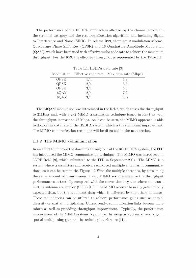
The performance of the HSDPA approach is affected by the channel condition,

the terminal category and the resource allocation algorithm, and including Signal

to Interference and Noise (SINR). In release R99, there are 2 modulation scheme,

Quadrature Phase Shift Key (QPSK) and 16 Quadrature Amplitude Modulation

(QAM), which have been used with effective turbo code rate to achieve the maximum

throughput. For the R99, the effective throughput is represented by the Table 1.1

Table 1.1: HSDPA data rate [3]

Modulation Effective code rate Max data rate (Mbps)

QPSK 1/4 1.8QPSK 2/4 3.6QPSK 3/4 5.3

16QAM 2/4 7.216QAM 3/4 10.7

The 64QAM modulation was introduced in the Rel-7, which raises the throughput

to 21Mbps and, with a 2x2 MIMO transmission technique issued in Rel-7 as well,

the throughput increase to 42 Mbps. As it can be seen, the MIMO approach is able

to double the data rate of the HSDPA system, which is the significant improvement.

The MIMO communication technique will be discussed in the next section.

1.1.2 The MIMO communication

In an effort to improve the downlink throughput of the 3G HSDPA system, the ITU

has introduced the MIMO communication technique. The MIMO was introduced in

3GPP Rel-7 [9], which submitted to the ITU in September 2007. The MIMO is a

system where transmitters and receivers employed multiple antennas in communica-

tions, as it can be seen in the Figure 1.2 With the multiple antennas, by consuming

the same amount of transmission power, MIMO systems improve the throughput

performance substantially compared with the conventional system where one trans-

mitting antenna are employ (SISO) [10]. The MIMO receiver basically gets not only

expected data, but the redundant data which is delivered by the others antennas.

These redundancies can be utilized to achieve performance gains such as spatial

diversity or spatial multiplexing. Consequently, communication links become more

robust as well as providing throughput improvement. Typically, the performance

improvement of the MIMO systems is produced by using array gain, diversity gain,

spatial multiplexing gain and by reducing interference [11].

4

Figure 1.2: A MIMO system. [1]

A wireless communication channel basically is not a perfect medium which intro-

duces fading to the received signal. The amplitude of received signal is corrupted

by random fading, which affect the reliability and the error rate of the received

symbol. Once a multiple antenna is employ at receivers or transmitters, a diversity

technique can be used to reduce the effect of the fading. The principle of the diver-

sity is to provide copies of a transmitted signal to receivers. Each signal reach to

the receiver after experiencing independent fading can be used to combine by using

signal processing techniques to provide more reliable transmission. This signal pro-

cessing method is called diversity processing and it can be done at the transmitter

side or at the receiver side. The diversity technique can be done on space, time or

frequency [12]. For example, coding and interleaving techniques may be used for

time diversity whilst a frequency diversity can be obtained by using filter at a trans-

mitter or a receiver. However, the time diversity and the frequency diversity appear

to be waste of resources to make use of the diversity. One more efficient method is

a space diversity [13] which can be done by separate antennas with proper space,

which is normally about a quarter of a carrier wave length to make independent

fading of received signals. In addition to space diversity, it is feasible to use an-

tennas with different polarization or use multiple antennas where each one point to

different direction for achieving the diversity. Signals travel through different paths

or polarization also encounters independent fading property.

The performance of the diversity technique can be indicated by array gain or

diversity gain [12]. The array gain represents how much average received SNR

increases, once the diversity is employed. The array gain can be formulated such

5

that [12]

ga =γoutγ

(1.1)

where γout and γ are an average of output SNR over channel distribution and average

of SNR output for a single branch respectively. The diversity gain is a negative slope

of the log-log plot of the average error probability versus the SNR, that is [12]

g0d(γ) = − log2(P )

log2(γ)(1.2)

where P is the average error probability.

Apart from using the MIMO technique to achieve diversity gain, it is also possible

to use the MIMO to improve data throughput as well. Under proper fading channel

conditions, the MIMO is able to transmit multiple data streams. At the receiver end,

each data stream can be separated as a single-input-single-output (SISO) stream,

which increases the data throughput proportionally to the number of transmitted

data streams. This is called spatial multiplexing technique [14]. Assume that there

are NT transmit antennas and NR receive antennas employed in the communication

and, by operating techniques such as a beam-forming, spatial multiplexing gain can

be produced as NL multiple substreams, where NL = min(NT , NR) is transmitted

simultaneously over a MIMO channel. With the parallel data stream transmission,

the bandwidth normalized capacity of the MIMO system is improved such that

C

BW= NL log2(1 +

NR

NL

S

N) (1.3)

The channel SNR is denoted by S/N while C and BW represents the channel capacity

and the channel bandwidth respectively. As this thesis aims to achieve the upper

bound capacity, the spatial multiplexing MIMO system is a major focus of the

thesis. The spatial multiplexing was originally introduced by [15] and have been

implemented in BLAST and V-BLAST system [16,17]

In addition, when using MIMO spatial multiplexing technique, a simple analyt-

ical system model was introduced in [15] to demonstrate that the level of noise in

each sub-stream increases. Especially, when the channel matrix becomes a singular

matrix, the level of noise is boosted greatly, yielding performance degradation as it

can be seen in (1.3). The reduction in the throughput due to co-channel interference

can be mitigated by using a MIMO interference reduction technique. In this con-

text, multiple streams received by the MIMO receiver are considered as interferer to

6

each other. The receiver firstly extracts the strongest signal and then subtracts this

signal stream from the rest of signal. Once the strongest signal is removed, the level

on the noise and interference in the remaining signal is reduced so that the receiving

process works more efficiently. The MIMO interference reduction technique can also

be operated in a multi-cell cellular environment to reduce the co-channel interfer-

ence caused by frequency re-using. In this case, the interference is reduced from

the margin of the expected signal by the co-channel signal but using this strategy

requires good knowledge of the channel information.

An example of the system which employs the MIMO communication is the IEEE

802.11n [18, 19].By exploiting MIMO and spatial multiplexing the data rate of the

IEEE 802.11 is increased. The IEEE 802.11n standard, when using 4 x 4 MIMO

with 4 spatial stream on 40 Mhz channel bandwidth, offers the peak data rate to

600Mbps [20], which is almost 12 times faster than the IEEE 802.11g.

1.2 Wireless Channel Fading

Naturally, communications using radio waves to transmit signals over long distances

will always encounter signal attenuation. The environments basically not only re-

duce amplitude of the transmitted signal but vary them randomly as well. The radio

transmission is based on the basic propagation principles of wave, reflection, diffu-

sion and scattering. Signals go to receiver appearing as a multiple reflection form

known as the multipath propagation. Each multipath reflection encounters ampli-

tude variation, known as fading or multipath fading that can harm or sometime

reinforce the received signal. In [21], fading characterized as a large-scale fading

channel, where receivers are moving over a large area. For large-scale fading, the

amplitude of the signal is not rapidly changing but gradually reducing as a propa-

gation distance increases. The large-scale model therefore emphasises on predicting

path loss coefficient as a function of the distance and environment factors. On the

other hand, when receivers are moving in a short distance, the amplitude of the

received signal fluctuates quickly so that small-scale fading model is used to de-

scribe the behaviour. In this model, the speed of the receiver or the transmitter and

multipath propagations influence the fading characteristics. Hence, the model can

be characterised by using the time-delay spread signal or a time-variance of signal,

as it can be seen in the Figure 1.3. The small-scale fading can be considered in a

time domain as well as a frequency domain. Moreover, it can be characterized as a

frequency selective fading channel, flat fading channel, slow fading and fast fading

7

Figure 1.3: Fading characterization. [22]

according the domain of operation. In this thesis focuses on the flat fading and

the frequency selective fading as we want to optimize the downlink throughput is

optimized for those channel models.

1.2.1 A MIMO Channel

Initial, MIMO channel modelling considered channel as the narrow transmission

band channel with the properties of independent and identical distribution (i.i.d)

flat fading channel. Later, the use of broadband communications is led to the use

of wideband model. This changes the common channel model to a broad spectrum

model, which is a frequency selective channel model. Moreover, extensive studies on

MIMO communications have demonstrated that MIMO channels basically have spa-

tial correlations between MIMO paths so that the analysis of MIMO communication

channel model required a more realistic model. The conventional MIMO channel

model for the system employing m transmit antennas and n receive antennas is given

8

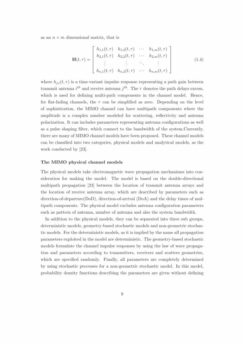
as an n×m dimensional matrix, that is

H(t, τ) =

h1,1(t, τ) h1,2(t, τ) · · · h1,m(t, τ)

h2,1(t, τ) h2,2(t, τ) · · · h2,m(t, τ)...

.... . .

...

hn,1(t, τ) hn,2(t, τ) · · · hn,m(t, τ)

(1.4)

where hj,i(t, τ) is a time-variant impulse response representing a path gain between

transmit antenna ith and receive antenna jth. The τ denotes the path delays excess,

which is used for defining multi-path components in the channel model. Hence,

for flat-fading channels, the τ can be simplified as zero. Depending on the level

of sophistication, the MIMO channel can have multipath components where the

amplitude is a complex number modeled for scattering, reflectivity and antenna

polarization. It can includes parameters representing antenna configurations as well

as a pulse shaping filter, which connect to the bandwidth of the system.Currently,

there are many of MIMO channel models have been proposed. These channel models

can be classified into two categories, physical models and analytical models, as the

work conducted by [23].

The MIMO physical channel models

The physical models take electromagnetic wave propagation mechanisms into con-

sideration for making the model. The model is based on the double-directional

multipath propagation [23] between the location of transmit antenna arrays and

the location of receive antenna array, which are described by parameters such as

direction-of-departure(DoD), direction-of-arrival (DoA) and the delay times of mul-

tipath components. The physical model excludes antenna configuration parameters

such as pattern of antenna, number of antenna and also the system bandwidth.

In addition to the physical models, they can be separated into three sub groups,

deterministic models, geometry-based stochastic models and non-geometric stochas-

tic models. For the deterministic models, as it is implied by the name all propagation

parameters exploited in the model are deterministic. The geometry-based stochastic

models formulate the channel impulse responses by using the law of wave propaga-

tion and parameters according to transmitters, receivers and scatters geometries,

which are specified randomly. Finally, all parameters are completely determined

by using stochastic processes for a non-geometric stochastic model. In this model,

probability density functions describing the parameters are given without defining

9

underlying geometry. Detailed and sets of example models of the MIMO physical

channel also are given in [23].

The MIMO analytical channel models

In the MIMO analytical models, mathematical methods are used to characterize

impulse responses of the channel. Each channel impulse response representing char-

acteristics of the path between transmit antennas and receive antennas and those

channel impulse responses are used to construct a MIMO channel matrix, which

is favorable for examining MIMO systems. The MIMO analytical models are cat-

egorized as propagation-motivated models, which characterize the matrix by using

propagation parameters, and correlation-based model, which take correlations be-

tween elements of the MIMO channel matrix into account. In this thesis, the em-

phasis is put on using the correlation-based models which the channel degradation

due to spatial correlation and antenna configurations are examined.

For the correlation-based models, the channel model is represented as a multi-

variate complex Gaussian distribution of the channels coefficient, and the MIMO

channel model is obtained as [23]

H =

√1

1 + KHs +

√K

1 + KHd (1.5)

where Hs and Hd are the matrices describing non-Line-of-Sight (non-LOS)and the

Line-of-Sight (LOS) component respectively, and K ≥ 0 denotes the rice factor.

In general, we are interested in the systems where the LOS component is absent

or K = 0, so that the MIMO channel matrix can be rewritten as H = Hs. The

channel matrix is a n×m dimensional matrix, where n and m represents a number of

antennas at the receiver and the transmitter. The channel comprises all multi-path

components. Hence, for time-varying channel, the MIMO channel can be represented

by discrete time channel impulse such that

H(t) =L∑

l=1

Hl(t)δ(t− l) (1.6)

L is a number of resolvable paths. It is further assumed that, there are no correlations

between multipath ray so that each Hl matrix can be modeled independently. In

the correlation-based model, the correlations of all entries in the channel matrix

are characterized by the full correlation matrix, RH , which is given for each lth

10

multi-path tap as

RH,l = Evec Hl vec HlH

(1.7)

Each element in the correlation matrix is a random variable and they are commonly

described by using the Laplacian [24] probability density function, which is basi-

cally formulated as a function of antenna configurations, Angle-Of-Arrival (AoA)

and Angle-Of-Departure (AoD). For simplicity, there are many schemes used to

calculate each correlation coefficients in the matrix RH . One of those approaches

is the i.i.d model that assumes all of elements in the MIMO channel matrix to

be uncorrelated. The i.i.d model can be applied on the rich scatter environment

where multipath components uniformly arrive at the receiver in all directions. The

correlation matrix therefore can be written as a function of a variance,ρ, which is

RH = ρ2I. Alternatively, the kronecker model [25] can be exploited to model the

correlated MIMO channel model. Using the kronecker model, the full correlation

matrix is given as a kronecker product, that is

RH = RTx ⊗RRx (1.8)

where RTx is a spatial complex correlation matrix of a transmit antenna array

whilst RRx denotes a spatial complex correlation matrix of a receive antenna array,

both correlation matrices represent correlation between the channel coefficients. For

the MIMO system, the channel capacity depends on the correlation between those

channel coefficients, where a large gain of the capacity can be achieved from a de-

correlated channel. The spatial correlation matrices are written as

RTx = EHHH

, RRx = E

HHH

(1.9)

Hence, for lth multi-path components, the kronecker model representing the MIMO

correlation channel Hl is given as

Hl = R1/2Rx,lHwR

1/2Tx,l (1.10)

The Hw is n × m dimension MIMO channel matrix whose entries are generated

from i.i.d complex Gaussian distribution. Note that, among the MIMO channels, the

kronecker model is the most successful model for examining the MIMO system. With

the feature that completely separates the transmitter and the receiver correlation

matrix, the model allows to perform optimization independently. This makes the

11

kronecker model favorite in MIMO system designing.

1.3 Research motivation

This section addresses the problems to be solved in the thesis

1. How to optimize energy efficiency and throughput in end-to-end

communication in the ad hoc networks.

Since energy is always a constrained resource in wireless networks, energy

efficiency is an important research topic in wireless communication. For high

speed networks, a data rates is directly proportional to the energy consumption

so that using the high data rate results in fast energy exhausting. For a given

transmission energy, what can be done in order to optimize the throughput

and the energy efficiency of the wireless network is to maximize the data rate.

This section shows optimizing energy efficiency and the throughput in ad hoc

networks, where the 3G-HSDPA technique is employed and the communication

channel is assumed to be a flat fading channel. The energy efficiency can be

optimized by using a multi-path routing communication collaborating with

a load balancing algorithm, which yields the extension of network lifetime.

Once the load balancing allocates the amount data to be transmitted to data

paths, the maximum throughput of the data paths then can be achieved by

using packet length optimization. It will be shown in the section that the

maximum throughput of the network is inversely proportional to a link service

time. Hence, the throughput will be improved by reducing the service time

when the slowest link data rate is maximized. For improving the slowest link

data rate, the MIMO communication can be implemented. The use of MIMO

changes the system to be MIMO-HSDPA integration system which requires

new resource allocation scheme.

2. How to allocate the total transmission energy into parallel coded-

channels of the MIMO-HSDPA system such that the upper-bound

throughput can be achieved

When maximizing the link data rate for the system with the HSDPA-MIMO

transmission technique, it is assumed that the total transmission energy per

symbol is limited at the transmitter. The HSDPA system uses multi-code

CDMA with orthogonal signature sequences, which spread the transmission

12

symbols. For a given signal to noise ratio at the receivers, the total capacity of

the system can be calculated. Currently, two methods are used to distribute

the total energy at the transmitter to achieve throughput close to the capacity

upper bound. These scheme are the equal-SNR-equal-rate (EEES) loading and

the equal-energy-equal-rate (EEER) loading scheme. The EEER is simple to

implement but at high SNR value the capacity diverge from the upper bound

capacity. The EEES produces a throughput close to the capacity upper bound

at the expense of having high computational complexity at the transmitter

and a high level of channel state information feedback requirement. Both

techniques will be applied on the HSDPA-MIMO to improve the downlink

throughput.

Simulation have been run to examine the performance of the EEER and the

EEES technique and it confirms that both schemes are able to provide the

promised results. However, it is necessary to evaluate the performance of both

techniques on practical systems. This section also includes the detail of setting

up the test bed system using the software defined radio based on the Labview-

FPGA system. Once the test bed system is constructed, it will be used to

examine the EEES and EEER approach and to produce the testing results for

the section.

3. How to deal with the correlated channel in the MIMO-HSDPA sys-

tem.

It will be assumed that the proposed wireless network operates in the envi-

ronment where the transmission scheme uses a MIMO link with signals being

correlated between the transmitter antenna elements and also between the

receiver antenna elements. This causes the communication channel becomes

correlated channel, which can be modeled by using A kronnecker model. The

Kronecker MIMO correlation channel model will be developed and the capac-

ity upper bound as a function of the received total signal to noise ratio will

be identified for the Kronecker correlated MIMO channel model. It will be

shown that the capacity for the correlated MIMO channels has a reduced or

degraded capacity. For the MIMO system with correlated channels, the CSI

feedback information is assumed to be perfectly known by the transmitter and

incorporates the correlation channel model to implement a pre-coder at the

transmitter to improve the degraded capacity. The pre-coding incorporating

with the resource allocation technique promises to improve the capacity over

13

the correlated channel. The performance of the proposed pre-coding technique

will be examined in the section.

1.4 Thesis outline

Chapter 2 discusses how to improve the end-to-end performance of the ad hoc net-

work. The chapter begins with the ad hoc system model and the description of the

physical layer to be used in the thesis. This section also includes the previous work

done on the physical layer to enhance the downlink throughput by using the HSDPA

with the two group bit allocation technique. Section 2 of the chapter demonstrates

how to enhance the energy efficiency by using the multi-path routing approach with

the load balancing algorithm. This section shows the results of the load balancing

which is used to extend the network lifetime. Then, the Carvalho’s MAC service

time model is discussed in section 3 of the chapter. This section also describes the

modification of the service time model for using in packet length optimization. The

validation and the simulation result of the new model is presented in section 4 of the

chapter. The modified service time is used to determine the optimum packets size.

When using the optimum packet size in data transmission, the end-to-end packet

delivery ratio is measured.

Chapter 3 introduces the use of the MIMO technique to increase the downlink

throughput of the 3G-HSDPA system. The first and the second part is for the

introduction and the related works. Section 3 of the chapter outlines the MIMO

system model to be employed in the chapter and the MIMO channel model which

is defined as a frequency selective channel. Section 4 describes the EEES and the

EEER resource allocation technique and the replicated simulation results produced

by LabVIEW. The detail of how the test bed system is constructed including the

time and frequency synchronization for the signal reception is given in section 5.

In section 6, the LabVIEW-PXIe test bed system used to produce the result for

the chapter is presented and, in the last part, the performance evaluation of the

proposed resource allocation technique is given.

Chapter 4 addresses the MIMO correlated channel problem. The first and the

second part of the chapter describe the MIMO correlated channel and the MIMO

system model to be used in the chapter, this part includes the kronecker model

and a method employed to formulate correlation coefficient matrices. The third

and the fourth section of the chapter discussed the capacity of the system and how

the correlated channel affects the capacity of the channel. The use of Eigen vector

14

pre-coding and the channel inverse pre-coding approach in order to improve the

capacity of the correlated channel is given in part 5 of the chapter and, in the

section 6, the performance of the Eigen vector pre-coding and the channel inverse

pre-coding system on the specified environment is discussed.

Chapter 5 contains the conclusion of the thesis and discusses about the future

work.

15

2 End-to-End Performance

Enhancement in Ad Hoc Wireless

Networks

Data throughput of networks is determined by the amount of information success-

fully transferred from a source to a destination in a given time. For a point-to-point

communication, the achievable throughput is the maximum throughput as data traf-

fic flow without any interruptions from surrounding environments. In this case, the

maximum throughput is only bounded by the physical layer parameters such as the

signal strength or a channel bandwidth. Typically, the maximum throughput or

the upper bound throughput can be obtained by using Shannon’s equation, which

gives the upper bound as the maximum data rate achieved by link. However, when

considering ad hoc networks, the throughput is not only depended on the physical

layer, it is also associated with other layer such as the link layer or the routing layer.

The link layer operates transmission scheduling tasks by using Medium Access

Control (MAC) protocols. For ad hoc networks, the Carrier Sense Multiple Access

with Collision Avoidance (CSMA/CA) protocol [26] is employed to organize trans-

mission and prevent data collision. The use of CSMA/CA protocol causes exchange

of overhead packets for establishing and securing the transmission session. Those

overhead packets are necessary but are not counted as real data so that, when ex-

amining the throughput of any individual links in ad hoc networks, the effective

throughput is utilized. The effective throughput is written as [27]

S =L

T(2.1)

where L is the data payload and T is a service time of the MAC protocol. The

service time T denotes time required to complete delivery of the packet containing

the data payload L, which include time for transmitting all overhead packets, time

spend by the MAC algorithm to solve collision problems in case they happen and

16

time for transmitting the data L

Data packets in ad hoc networks are usually not transmitted directly from sources

to destinations due to limitation of radio signals. The packets are actually delivered

in a multi-hop fashion via intermediate nodes between the source and the destination.

A multi-hop path is selected by a routing layer based on goals networks want to

achieve. For instance, the path might be selected to minimize latency or to optimize

the throughput. Once communication is run on a multi-hop path, the performance to

be considered here is the maximum end-to-end throughput. Data packets traversing

the multi-hop path basically encounter different service time from each intermediate

node. The service time really varies and depends on the network topology and

traffic load at that time. For a given multi-hop data path, the maximum end-to-end

throughput can be obtained as [28]

S = minji=1S1, S2, , . . . , Si (2.2)

where j is the maximum number of hop length in the path and Si represents effective

throughput of the intermediate node i, given in (2.1). Since the service times are

different among nodes in the path, the effective throughput of each node is not

equal. The maximum end-to-end throughput on the path is limited by the slowest

link, known as the bottleneck link, where the service time of the link is the maximum.

This work concentrates on optimizing end-to-end throughput and energy efficiency

ad hoc networks. The ad hoc network uses a multipath routing approach to trans-

mit data in order to achieve target end-to-end throughput whilst optimize energy

efficiency. The multi-path routing algorithm is formulated as a cross-layer optimiza-

tion, where a parameter determined at the physical layer is utilized to identify a

set of disjoint data paths link between source nodes and destination nodes.Once

the multi-path communication is established, data bits will be allocated into each

data path such that the required throughput can be achieved. Giving the total

throughput as M bps, M bits of data is going to be loaded into all data paths

in each second. Since energy consumed by each path is different, data bit allo-

cated into each path must be distributed so that the total energy consumed by

each path is in balance. The data bit to be loaded into each path is determined

by the load balancing algorithm. For giving a set of path Jz for z = 1 , . . . , Z

data bit to be allocated to path Jz is determined as mz, which yields total energy

consumption on the path jz is written as Ez = mzEb,z, where Eb,z is energy re-

quired to transmit one bit of data. Hench, energy consumed by each path is written

17

as m1Eb,1 = m2Eb,2 = , . . . , = mzEb,z = , . . . , = mZEb,Z , which maximize the

network lifetime as well as energy efficiency.

After data bits are allocated, the optimal packet size has to be determined in

order to maximize the throughput. Giving the data packet as L, the optimal packet

size for data path z can be calculated as

Lz =mz

Tmaxi,l∈Jz

(T i,l) (2.3)

Where maxi,l∈Jz(T i,l) is the maximum service time of path z. As it can be seen,

in order to determine the throughput, the maximum service time is required.This

chapter mainly focuses on modeling the link service time, which is re-

quired to determine the optimal packet size. The service time model

need to be tested on the interesting network and modified properly, so

an accurate service time value can be obtained.

The service time is a parameter of the MAC protocol and the standard MAC pro-

tocol for ad hoc networks, the IEEE 802.11 with Distributed Coordination Function

(DCF) mode, is used in this chapter. The IEEE 802.11 employs the CSMA/CA algo-

rithm to perform data transmission and the binary exponential backoff algorithm [29]

to deal with data collision problems. For networks using the IEEE 802.11 protocol,

the service time of each node can be estimated by the Carvalho’s model [30]. The

model calculates the service time based on saturated network assumption, which can

be adapted to be used in determining the service time of multipath communication.

At the physical layer, the WCDMA with single code communication is employed

in transmission. However, it was shown in [31], the single code communication in

ad hoc networks is not energy efficient, and it can be improved by using the HS-

DPA approach with two-group energy allocation, which effectively spends residual

energy to increase physical data rates. Since the data rate is higher, the service time

decreases. Consequently, the end-to-end throughput is enhanced, as it is inversely

proportional to the maximum service time of a given data route. The end-to-end

throughput can be further increased by applying a MIMO-HSDPA technique. The

use of MIMO communication substantial increases in data rates. Therefore, the

end-to-end throughput can be maximized.

This chapter is organized as follows. In the section 2, the ad hoc system model

is described, which includes descriptions of the physical layer and network topol-

ogy. The energy efficiency multi-path routing protocol is discussed in the section 3

whilst The IEEE 802.11 MAC protocol and the Carvalhos service time model are

18

detailed in the section 4. In section 5, the model validation and simulation results

produced by the NS-2 network simulator [32] are given, including the discussion.

The section 6 summarizes on the work and contribution in this chapter and also dis-

cusses the potential of using MIMO-HSDPA technique in order to further improve

the performance of the systems.

2.1 Ad Hoc System Model and the Physical Layer

Description

First of all, the topology of ad hoc networks to be simulated and all definitions used in

the model are described. The model gives an overview of how nodes in the networks

are connected and how they communicate to each other. After that, description of

the physical layer will be given. This includes the wireless communication techniques

according to the standard IEEE 802.11 and the HSDPA multi-code communication

using in the physical layer enhancement.

2.1.1 Network Topology and the Description of The System Model

A regular ad hoc network consists of a number of nodes deployed in a flat plain

area. The term flat explains that all nodes are located on the same level or their

heights are considered to be equal. It is assumed that the network is stationary

so that all nodes stay at a fixed coordinate over simulation period. It is assumed

that all nodes are equipped with a radio transceiver in order to transmit data using

wireless communication, where an electromagnetic wave with frequency f , given in

Hz unit, is used as a carrier. The carrier wave is transmitted by a transmitting

antenna, which ht denotes the transmitting antenna height. Similarly, the antenna

with the height of hr is used to receive the signal. When using wireless communi-

cation, the received signal strength can be estimated by using a radio propagation

model and, in this work, it is initially assumed that signal traverses a flat fading

channel. The received signal therefore suffers from only a propagation loss, where

the loss factor is given in [33], will be discussed in the next section. In addition,

the noise encountered at received signal is modeled as Additive White Guassian

Noise (AWGN). The AWGN noise power is formulated as a function of transmission

bandwidth and temperature, as given in [27]. Each node consumes energy supplied

by a battery and total transmission energy per symbol period is fixed to be ET .

At the receivers, if the received signal strength is sufficient for the transmitter to

19

send data packets with the minimum data rate, defined as the minimum number of

bits per symbol allowed by the transmission technique, it can be said that there is

a communication link between the transmitter and the receiver. To put it simply,

transmission energy is set such that every node can transmit data in free space up to

200 metres around themselves, or the maximum transmission distance is equal to 200

metres. According to the IEEE 802.11 standard, a MAC protocol is used in packet

transmission. When employing a MAC protocol, it is necessary to set the carrier

sensing range representing the maximum range that nodes can detect any packet

transmissions happen within. Nodes hearing the transmissions then are forced to be

idle till the transmission is completed, which prevents the existing communication

from any interruptions created by surrounding nodes. The carrier sensing range

used in this work is the optimum range given by [34],which double of the maxi-

mum transmission distance (400 metres).By using aforementioned assumption, the

example network topology containing 50 nodes can be created as demonstrated by

Figure 2.1.

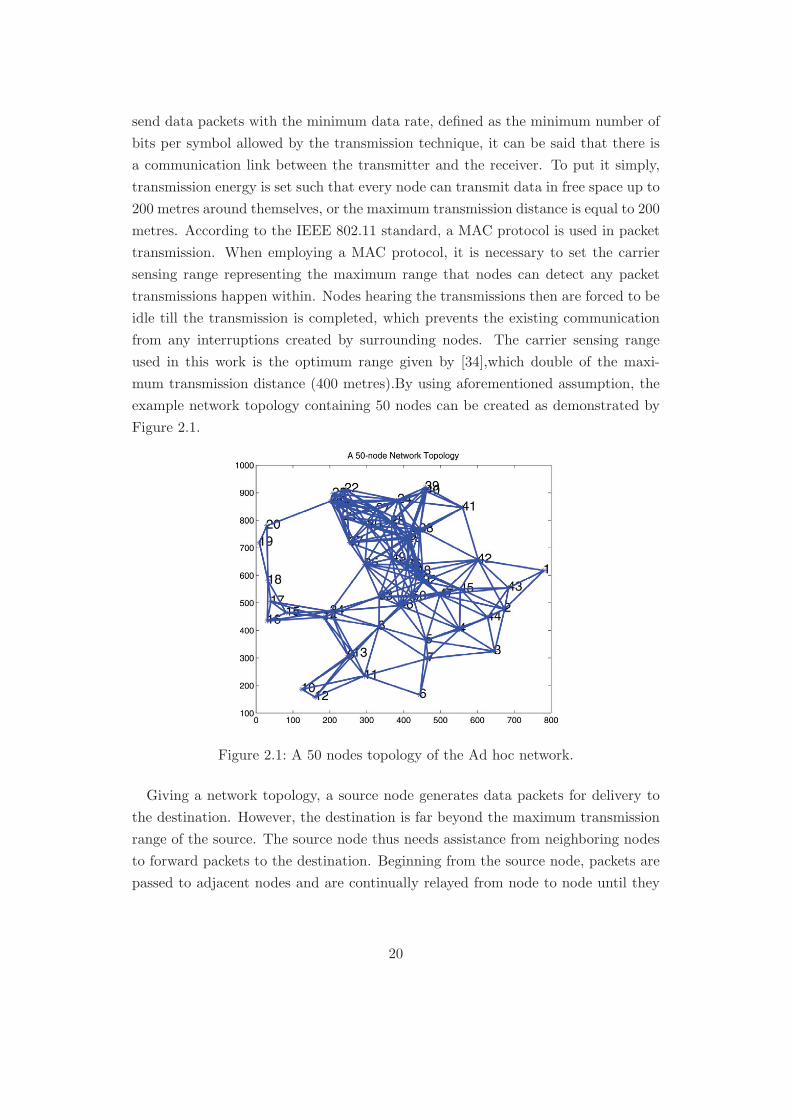
Figure 1 : 50 nodes ad hoc network Figure 2.1: A 50 nodes topology of the Ad hoc network.

Giving a network topology, a source node generates data packets for delivery to

the destination. However, the destination is far beyond the maximum transmission

range of the source. The source node thus needs assistance from neighboring nodes

to forward packets to the destination. Beginning from the source node, packets are

passed to adjacent nodes and are continually relayed from node to node until they

20

are received by the destination. Set of nodes involved in the packet transmission is

call data path and, for the ad hoc network, the data path is defined as a multi-hop

path. It can be said that the multi-hop path is established from a set of nodes

where each member of the set connects to at least one member in the set. If the

number of nodes contained in the network is high enough and the nodes are deployed

properly, it is possible to have many data paths link between the source node and the

destination node and all of them can be used to deliver data packets, which is known

as a multi-path communication. It is assumed that data paths participating in the

packet transmission must be disjoint paths in which nodes comprising each path

are totally different, apart from the source and the destination. The set of disjoint

paths to be used can be identified by the multipath routing algorithm called the hop

trellis diagram, which is described later in the next subsection.Once a group of data

path is established for packet transmission the source node allocates packets to each

data path such that energy consumption across the network is equally distributed

and a target end-to-end throughput is satisfied. The end-to-end throughput for the

data path can be determined by using (2.2), which requires the MAC’s service time

in the calculation. The Carvalho’s model [30] is used to determine the service time

in the end-to-end throughput examination.

2.1.2 Channel Modelling for Ad Hoc Networks

A carrier signal transmitted by nodes propagates across space and it typically en-

counters many objects spoiling quality of the signal before reaching a receiver. The

signal power basically is absorbed by atmosphere, signal strength is attenuated as

it travels further away from the transmitter. Parameters such as temperature or

humidity affect the signal, which creating noise and causing fluctuation in the am-

plitude of received signal. If there is a Line-of-Sight (LOS) path where signal can

travel on a straight line from a transmitter to a receiver, the received signal might not

be attenuate significantly over the paths. However, in most communication systems,

non-line-of-sight paths usually exist and signals go to a receiver in accordance with

the propagation mechanism, reflection, diffraction and scattering. Consequently, the

received signal is always distorted, which limits the performance of the communica-

tion link.

The signal propagation can be predicted by a channel model. For ad hoc networks,

the channel model can be simple or very complicated depending on factors to be con-

sidered such as propagation characteristics, location of the network or network type.

21

Basically, the wireless channel can be characterized as 2 major forms, the large-scale

or path loss model and the small-scale or fading model [35]. The large-scale model

normally is employed to estimate signal attenuation as a function of transmitting

distance. Using the large-scale model gives the average received signal strength,

which eventually reflects the coverage area associated with the transmitter. The

amplitude of the received signal however does not only experience the attenuation,

it also encounters rapid variations as well. This is because the received signal is

actually a combination of multiple signals appearing at the receiver in an observa-

tion period. The multiple signals take different NLOS paths for traveling, causing

different phase and delay time when they reach the receiver. Hence, once they are

added together, the resulting signals might have fast changing amplitudes. The

rapid variation is called multi-path fading effect and it typically can be described by

using the small-scale fading model. It can be said that the received signal strength

measured at different transmission ranges vary widely due to multi-path fading, but

mean value of the signal strength decrease as the transmission range increase. Both

propagation model therefore are essential for signal strength prediction.

In this work, it is assumed that the multi-path fading have small effects on the

received signal strengths. Therefore, only the large-scale model is employed when

calculate the received signal strength. The path loss factor utilized to estimated

received signal is taken from [33]. The path loss model is formulated based on free

space model [35] and take into account the height of antennas, as it creates Fresnel

zone loss which reduce transmission distance of carrier wave given in gigahertz (GHz)

band. The proposed model gives an approximation for a path loss factor in ad hoc

systems where low height antennas are exploited in transmission. The path loss

factor is given as

h = 40log10d + 20log10f − 20log10hrht (2.4)

where d is the separation distance between the transmitter and the receiver, given

in metres unit. f denotes the carrier frequency in Gigahertz (GHz) while hr and ht

represent the height of the receiving antenna and the height of transmitting antenna

respectively. Giving a carrier frequency 2.45 GHz and hr = ht = 1.5 metres, the

loss factor can be rewritten as a function of the distance d as follows

h = 40log10d + 0.736 (2.5)

By using (2.5), the expected received SNR corresponding to the distance d can be

calculated as tabulated in table 1. Note that, interference is ignored and transmission

22

power and noise power used in the calculation are 5 dBm and -90 dBm respectively.

Table 2.1: Path loss calculation

Transmission range (metres) Path Loss (dB) Received SNR (dB)

1 m 0.736 94.2645 m 28.69 66.3115 m 47.78 47.2250 m 68.69 26.31100 m 80.736 14.264150 m 87.78 7.22200 m 92.78 2.22

2.1.3 Received SNR Calculation

Originally, the IEEE 802.11 standard assigned a code division multiple access (CDMA)

for data transmission. With the CDMA scheme, data is spread by code sequences

to create a wide band signal before transmission. The objective is reduced spectral

energy for each signal which allows more data stream to be transmitted in parallel on

the same frequency. At the receiver, since the used spreading codes are orthogonal,

each data stream can be easily extracted by using the same code sequence to de-

spread. The IEEE 802.11 can use CDMA with two spreading technique, Frequency

Hopping Spread Spectrum (FHSS) and Direct Sequent Spread Spectrum (DSSS).

The FHSS approach transmits data over a carrier changing frequency band peri-

odically. The frequency of a carrier is selected corresponding to hopping pattern

generated by a pseudorandom code generator. The received signal appears to be

transmitted over random channels and can be detected, if the receiver synchronizes

with the transmitter and knows the hopping sequence. In this work, we focus on

the DSSS approach which uses code sequences to spread data to be transmitted di-

rectly. Traditionally, the spreading sequence consists of a set of rectangular pulses,

which each pulse can be called ”chip” and has a pulse width of Tc. Assuming data

to be transmitted are generated as symbols with a bandwidth of Bs and a symbol

period of Ts. Once these symbols are passed to the spreading process, the spreading

sequence distributes the symbol power over the bandwidth Bss, where Bss ≫ Bs,

before the transmission. At the receiver, the received signal are corrupted by inter-

ference power over the entire Bss bandwidth. However, the de-spreading process can

23

recovers the transmitted symbols into the Bs bandwidth whilst leaving interference

power be scattered. As a result, the majority of the interference surrounding the

bandwidth Bs can be easily removed by using a bandpass filter. The performance of

the DSSS approach can be determined by the interference rejection ratio or it can

be called as the processing gain (PG), which is written as

PG =Ts

Tc(2.6)

Assuming that each node in ad hoc networks employs a DS-CDMA transmission

technique for communication. The system operates the DS-CDMA approach using

spreading sequences with length of NPG chips, where each chip has a pulse duration

of Tc. Node i equipped with a single antenna, whose height is fixed at ht, to transmit

data to node l, which employing antenna with height of hr to receive the data. The

distance between node the i and the node l is given as di,l and a carrier wave signal

is transmit at the centre frequency f . At node i, each symbol is generated with a

symbol period of Ts and is transmitted with the maximum transmission power PT .

Therefore, the energy required for transmitting in each symbol period is given as

ET = TSPT or it can be rewritten as ET = NPGTcPT , as each symbol is spread

by a spreading sequence. At node l, since multi-path fading is not considered, the

received signal energy can be calculated as

PR = 10−h/10ET (2.7)

where h is obtained from (2.4). For the signal-to-noise ratio (SNR) estimation, it

is assumed that the noise corrupting the system is the AWGN noise, as described

in section 3.2.1. The AWGN noise can be modelled by the normal distribution

with zero mean value and σ2 variance, which gives the noise power as N0 = 2σ2.

Therefore, the received SNR can be determined by using the following equation

SNTtotal =10−h/10ET

N0(2.8)

Once the received SNR is obtained, the data rate can be estimated according to

resource allocation techniques, which is going to be discussed later.

24

2.1.4 Data Rate Calculation in Single-Code CDMA Systems

A data rate corresponding to a given received SNR can be estimated by using Shan-

non’s equation. For a theoretical system where no error rate is taken into consid-

eration, the achievable data rate is known as the upper bound rate and is written

as

b = log2(1 + SNRtotal) (2.9)

where b is given in bits/symbol. However, in practice, the systems always suffer

communication channel impairment which result errors in the received data. In

order to reflect the actual performance, equation (2.9) is rewritten as

b = log2

(1 +

SNRtotal

Γ

)(2.10)

where Γ is a gap value introduced to measure the different between the theoretical

system and practical systems. The theoretical data rate for a given total SNR is

provided by (2.9). Alternatively, because of the presence of the errors, obtaining

the same rate b in practical systems needs higher SNR. The difference of SNR value

between both systems is represented by the gap value Γ, given in dB unit. It is

obvious that the Γ must be minimized so that the upper bound can be achieved.

Traditionally, channel coding techniques are used to reduced the errors in received

data, which is defined as the Bit-Error-Rate (BER). There are two types of channel

coding which is currently in use, the block coding approach and the convolutional

coding approach. The block coding such as a Low-Density-Parity-Check (LDPC)

approach [36] concatenates on code word, which has redundant information, with

data placed into a block. On the other hand, a convolutional coding schemes as

well as a turbo coding techniques [37] encode data as a stream rather than a block

code. Both techniques have different in complexities and performance and the choice

depend on specific systems. Basically, the standard of HSDPA needs BER up to

10−3 and the turbo coding approach is used for the channel coding. For application

required a low BER, which is in range 10−6 < BER < 10−3 [38], the convolutional

coding is performed instead. In this work, we assume that application requires very

low BER so that the BER of 10−6 is set for the simulation, which corresponds

to 8 dB of the gap value, where the gap value is defined in [39]. In data rate

calculation for each transmission technique, adaptive modulation and coding scheme

(AMC) is utilized. The AMC selects a data rate and coding technique based on the

received SNR. Therefore, the system operates with available discrete bit rates bp for

25

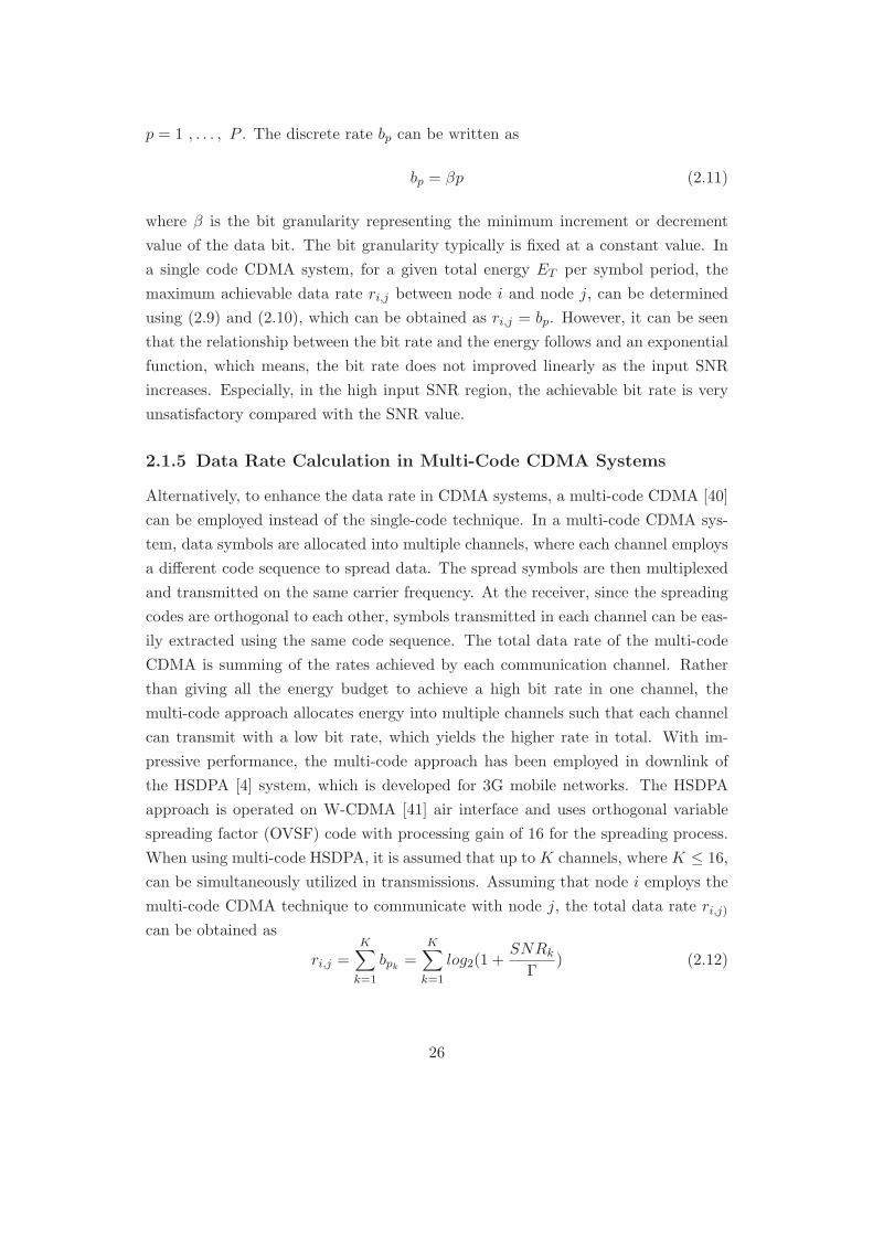
p = 1 , . . . , P . The discrete rate bp can be written as

bp = βp (2.11)

where β is the bit granularity representing the minimum increment or decrement

value of the data bit. The bit granularity typically is fixed at a constant value. In

a single code CDMA system, for a given total energy ET per symbol period, the

maximum achievable data rate ri,j between node i and node j, can be determined

using (2.9) and (2.10), which can be obtained as ri,j = bp. However, it can be seen

that the relationship between the bit rate and the energy follows and an exponential

function, which means, the bit rate does not improved linearly as the input SNR

increases. Especially, in the high input SNR region, the achievable bit rate is very

unsatisfactory compared with the SNR value.

2.1.5 Data Rate Calculation in Multi-Code CDMA Systems

Alternatively, to enhance the data rate in CDMA systems, a multi-code CDMA [40]

can be employed instead of the single-code technique. In a multi-code CDMA sys-

tem, data symbols are allocated into multiple channels, where each channel employs

a different code sequence to spread data. The spread symbols are then multiplexed

and transmitted on the same carrier frequency. At the receiver, since the spreading

codes are orthogonal to each other, symbols transmitted in each channel can be eas-

ily extracted using the same code sequence. The total data rate of the multi-code

CDMA is summing of the rates achieved by each communication channel. Rather

than giving all the energy budget to achieve a high bit rate in one channel, the

multi-code approach allocates energy into multiple channels such that each channel

can transmit with a low bit rate, which yields the higher rate in total. With im-

pressive performance, the multi-code approach has been employed in downlink of

the HSDPA [4] system, which is developed for 3G mobile networks. The HSDPA

approach is operated on W-CDMA [41] air interface and uses orthogonal variable

spreading factor (OVSF) code with processing gain of 16 for the spreading process.

When using multi-code HSDPA, it is assumed that up to K channels, where K ≤ 16,

can be simultaneously utilized in transmissions. Assuming that node i employs the

multi-code CDMA technique to communicate with node j, the total data rate ri,j)

can be obtained as

ri,j =K∑

k=1

bpk =K∑

k=1

log2(1 +SNRk

Γ) (2.12)

26

where k is the indices of channel and k = 1 , . . . , K. It is assumed that a channel is

a flat fading channel, each sub channel k encounters the same path loss and noise.

The amount of energy required to achieve the maximum bit rate bp of bit per symbol

in the channel k is formulated as

Ek(bp) =N0Γ

10−h/10(2bp − 1) (2.13)

As the channels experience the same conditions, the required energy Ek(bp) is equal

in all channels. The total energy consumption is obtained as KEk(bp) and it must

not excees the energy budget, the available transmission energy per symbol period

ET , such that KEk(bp) ≤ ET . With this energy consumption, the total bit rate

between node i and node l is given as follows

ri,l = Kbp (2.14)

In order to increase the bit rate in all channels to one step higher, bp+1, the system

requires total energy of KEk(bp+1). Since bp is the highest possible achievable bit

rate, obtaining the bp+1 in all channels result over energy budget, which can be

demonstrated by the inequality as follows

KEk(bp) ≤ ET < KEk(bp+1) (2.15)

However, in careful analysis, it found that loading data bit equally contributes to

waste of transmission energy. Once transmission energy is allocated to get the

maximum bit rate bp, there is remaining transmission energy which is not spent as

it is insufficient to use in increasing the data rate to bp+1 in all channels. This energy

is called the residual energy, which can be demonstrated as the following equation

0 ≤ ǫR = ET −KEk(bp) < K(Ek(bp+1) − Ek(bp)) = Kǫ(bp) (2.16)

the residual energy, ǫR, is bound by Kǫ(bp) , which increases as more parallel channel

is performed. The ǫ(bp) is called the incremental energy which is required to improve

the data rate such that the rate bp increases by β for p = 1 , . . . , P − 1. The

incremental energy is given as

ǫ(bp) = Ek(bp+1) − Ek(bp) =N0Γ

10−h/10(2β − 1)2bp (2.17)

27

The presence of the residual energy confirms that energy is not utilized effectively

and it is necessary to reduce the residual energy for the performance improvement.

The work reported [31] examined the residual energy and proposed a method to

exploit the residual energy to improve the total data rate, which is called two-group

resource allocation. The two-group bit loading uses residual energy to increase the

bit rate in potential channels. As a result, the communication channels are separated

in two groups, where one group is loaded by a higher bit rate. The two group resource

allocation therefore minimizes the residual energy whilst optimizing the total data

rate.

2.1.6 Two-Group Bit Allocation in Multi-Code CDMA Systems

Giving total number of communication channel as K, by using the two-group ap-

proach, m channels are allowed to transmit with a bit rate bp+1 whilst K−m channels

transmit with a bit rate bp, which is a lower bit rate. The total transmission rate

hence is obtained as

ri,j = (K −m)bp + mbp+1 (2.18)

where m is the integer number with the value giving between 1 and K−1. The total

transmission energy required by the two-group approach is equal to (K−m)Ek(bp)+

mEk(bp+1). The residual energy of the two-group can be rewritten as

0 ≤ ǫR = ET − ((K −m)Ek(bp) + mEk(bp+1)) < ǫ(bp) (2.19)

the residual energy gradually decreases as the number of m channels increases and

, when m reaches the maximum value, it can be seen that the upper bound of the

residual energy is reduced substantially by a factor of K.

To allocate data bits, the two-group bit loading algorithm requires to calculate

only the rate index p for getting bit rate of the low group channel, bp. Then, the

number of high group channel, m, is estimated such that the residual energy is

minimized. For a set of given parameters ET ,K, h,N0,Γ, β and the discrete bit rate

set bp for p = 1, . . . , P the index p can be calculated by using the following equation

p = min

log2

(10−h/10ET

KΓN0+ 1

)

β

, P

= min

log2

(SNRtotal

KΓ + 1)

β

, P

(2.20)

Once the bit rate bp is obtained, the number of high group channel m can be deter-

28

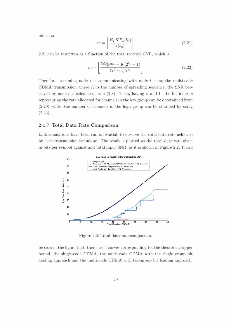
mined as

m =

⌊ETKEk(bp)

ǫ(bp)

⌋(2.21)

2.21 can be rewritten as a function of the total received SNR, which is

m =

⌊SNRtotal

Γ −K(2bp − 1)

(2β − 1) 2bp

⌋(2.22)

Therefore, assuming node i is communicating with node l using the multi-code

CDMA transmission where K is the number of spreading sequence, the SNR per-

ceived by node l is calculated from (2.8). Then, having β and Γ, the bit index p

representing the rate allocated for channels in the low group can be determined from

(2.20) whilst the number of channels in the high group can be obtained by using

(2.22).

2.1.7 Total Data Rate Comparison

Link simulations have been run on Matlab to observe the total data rate achieved

by each transmission technique. The result is plotted as the total data rate given

in bits per symbol against and total input SNR, as it is shown in Figure 2.2. It can

Figure 2.2: Total data rate comparison.

be seen in the figure that, there are 4 curves corresponding to, the theoretical upper

bound, the single-code CDMA, the multi-code CDMA with the single group bit

loading approach and the multi-code CDMA with two-group bit loading approach.

29

The upper bound curve is obtained by using (2.7). Apart from the upper bound,

each curve is calculated from a set of parameters including β = 2, Γ = 7.8 dB and

bp ∈ 2, 4, 6. For a single-code CDMA, the required SNR to achieve each bit rate

is determined as γ∗(bp) = Γ(2bp − 1). Since there is only 3 available discrete bit

rates, the curve of the single-code CDMA approach represents as three step. The

maximum data rate is saturated and remains at 6 bits per symbol, although the SNR

increase beyond 30 dB. For the multi-code CDMA approach, it is assumed that only

3 sets of spreading sequences can be employed according to the HSDPA standard,

where each code set has different number K of spreading code. The number of code

corresponding to each spreading sequence can be represented as a set where K ∈5, 10, 15. The total data rate of the multi-code CDMA is given as r∗(bp) = Kbp

while the SNR required for each bit rate is obtained from γ∗(bp) = K(2bp − 1).

Given the set of K and the set of bp, The total data rate of the multi-code CDMA

is obtained by maximizing K and bp whilst satisfying the input SNR γ∗. From the

figure, it can be observed that having the multi-code CDMA technique enhances

the total data rate significantly. Especially, in the high SNR region, the results

show that the multi-code approach is much better than the single-code approach.

However, the throughput of the multi-code scheme also has a step, because the

approach contributes to waste of the input SNR. The residual SNR can be measured

from width of each step in the curve. A further performance improvement can be

achieved by using the two-group bit allocation approach. The curve of the two-group

bit allocation is higher than the others for all input SNR values. Moreover, the curve

grow smoothly as the input SNR increase, which means that the residual energy is

utilized wisely to improve the total data rate.

Once the physical layer is enhanced by the two-group approach, it is possible

set the improvement by optimizing the other layer. Next, the multi-path routing

approach developed by using a cross-layer optimization will be discussed. The multi-

path routing technique searches for a set of disjoint paths which have been to develop

to minimize transmission energy and to improve the network energy efficiency.

2.2 Routing Layer and an Energy Efficiency Routing

Algorithm

Since batteries are the main energy supply for ad hoc networks, energy is limited

and important resource, which needs to be used wisely in order to extend the life

30

time of the networks. The last section has discussed the physical layer enhancement

which aims to minimize the residual energy and to increase the total data rate.

The implementation of the technique ensures that each individual link consumes

transmission energy effectively. However, when the links are operated as a network,

achieving energy efficiency needs to take more factors into consideration.

Consider an ad hoc network, a source node in which requests the network to con-

struct a data path for packet delivery. Once the data path is established, packet

transmissions are replicated only on that path to preserve network goal such as mini-

mizing the latency or maximizing the end-to-end throughput. As a result, the energy

of nodes placed in a long data path are therefore exhausted quickly, which cause the

network life to be shorted as nodes will exhaust the energy. Therefore, a single path

communication may not be suitable when considering the network life time and en-

ergy balancing.Instead of using a single path communication, suggested in [42], a

multi-path routing approach can be employed to improve the network performance.

The multi-path routing can enhance both end-to-end throughput and energy effi-

ciency as studied in [43–45]. In [43], the multi-path routing is used to improve the

successful delivery ratio. The work demonstrated that the performance of networks

increases as more data paths are used in data transmissions. Unlike [43], the multi-

path routing is used to improve the energy efficiency as shown in [44] and [45]. The

objective of both works is to improve the average network life time by distributing

energy consumption uniformly over all available routes. In work [44], the number of

node placed in the data paths is taken into account for calculating the number of

packet to be allocated into the path. Alternatively, work [45] considers sum of the

remaining energies in the batteries of the path for the packet allocation. Both work

spread data load over a group of paths as well as energy consumption. As a result,

the average network life time can be extended. The multi-path routing approach

therefore can be applied in this work to optimize the end-to-end throughput and en-

ergy utilization as well. When using a multi-path routing approach, path selection

have a great impact on the performance of the system. For network optimization per-

formance, matrices which may be considered include latency, throughput or lifetime.

The path selection may take parameters from others protocol layers into account,

which is known as a cross-layer optimization. As given in [46], signal strength, which

is a parameter of a physical layer, is used in the path selection. The objective is

to search for robust paths to deliver packets, which minimizes latency due to link

failure during the transmission. On the other hand, the path selection may consider

parameters provided by the MAC protocol, as demonstrated by [47]. This routing

31

algorithm is classified as an opportunistic routing where the packets are forwarded

according to transmission success rate. For a multi-path routing approach, a group

of disjoint paths, which each data path has no common nodes or common links ex-

cept the source and the destination, can be employed. As conducted by [48], the

routing algorithm should select a set of disjoint paths for multi-path communication.

Hence, path conflicts and data collisions can be reduced.

In this work, a multi-path routing approach with a load balancing algorithm is

employed. The aim of using the multi-path communication is to satisfy the target

end-to-end throughput and to maximize the network life time. The multi-path rout-

ing algorithm is formulated using a physical-routing cross layer aspect, where data

path selection is based on a physical parameter called the bit-energy consumption.

For each physical link, the bit-energy consumption represents energy required to

transmit one bit of data, which is inversely proportional to the link data rate. The

multi-path routing algorithms search for a set of least-cost disjoint paths, where

summing of the bit-energy consumption in each path is the smallest. The packet

transmission hence can be operated with the minimum transmission energy. In addi-

tion, a load balancing algorithm [49] is also implemented to ensure that the network

life time is maximized. The algorithm allocates amount of data into each path such

that the energy consumption is identical. The complexity of the multi-path routing

algorithm is one of the major concerns. Originally, the route discovery algorithm

used in this work is called the hop trellis diagram [50], which contribute to complex-

ity of O(N2) in discovery all usable paths. In order to reduce the complexity, the

modified Viterbi algorithm is applied on the hop trellis diagram. The complexity of

the hop trellis diagram and the modified Viterbi algorithm is investigated by [51],

it demonstrate that the complexity of the multi-path routing algorithm is improved

and drop to O(N) when using the modified Viterbi algorithm.

The formulation of the bit-energy consumption is outlined in the next section.

After that, the description of the trellis-hop diagram, the modified Viterbi algorithm

and the load balancing algorithm will be given.

2.2.1 Minimizing Energy Consumption Using Bit-Energy

Consumption

When employing the transmission techniques proposed in section 2 in ad hoc net-

works, data rates are calculated as a function of transmission distance. The data

rates, measured in bits per symbol, of each link is changed across the networks,

32

although the transmission energy per symbol period is allocated equally. This also

means giving those links the same amount of data bits to transmit, high speed links

consume less transmission energy, as a number of transmitted symbols is lower.

Hence, bit energy consumption defined as energy required for transmitting one bit

of data can be used as a metric to compare energy efficiency of each link. Similarly,

the bit energy-consumption can be employed in the multi-path routing algorithm to

identify the least-cost path where the sum of the bit-energy energy consumption is

the smallest so that it can guarantee that each path consumes the minimum energy

in packet transmissions.

Assuming an ad hoc network consisting of N number of nodes is randomly de-

ployed on a space. The number of nodes N is large enough so that each node

connects to at least one node in the network. For a given source node and a desti-

nation node, a set of disjoint paths is discovered for the packet transmission. The

maximum number of disjoint paths employed in the transmission is given as Z and

a set of nodes comprise each path is denoted by Jz where z = 1 , . . . , Z. The ad

hoc network needs to transmit M bits of data over all routes whilst each route is

allowed to carry a total of mz bit of data. Hence, M =∑Z

z=1mz. For the trans-

mission, the network employ the CDMA technique with the chip period of Tc and

the processing gain of NPG. The transmission power for each node is fixed equally

at PT . Since the symbol is spread by the chip sequence, the symbol period is ob-

tained as Ts = NPGTc and the transmission energy per symbol period is written as

ET = PTTs = PTNPGTc.

For every node i and node l where i, l ∈ Jz, the energy ET is consumed for the

transmission and, having this transmission energy, communication between node i

and node l achieve a data rate of ri,l bits per symbol. Since the path Jz delivers mz

bits, each link i, l transmits up to mz/ri,l symbols. Therefore, the energy required

by link i, l to send mz bits can be calculated as

Ei,l,z =ETmz

ri,l(2.23)

The total energy that path Jz consumes for deliver the data mz is given as

Ez = mzET

∑

i,l∈Jz

1

ri,l= mzPTNPGTc

∑

i,l∈Jz

1

ri,l(2.24)

33

from 2.24, the bit energy consumption is determined as

Eb,z = PTNPGTc

∑

i,l∈Jz

1

ri,l(2.25)

It can be seen that the bit energy consumption is inversely proportional to the data

rate. Hence, the bit energy consumption can be reduced by improving the data

rate. It is obvious that energy the consumption in multi-path communication can

be minimized by selecting a set of path corresponding to the lowest Eb,z. The Eb,z

is then employed as a cost metric for the multi-path routing algorithm.

2.2.2 The Load Balancing Algorithm

Once a set of data paths is discovered, the amount of data carried on each path

need to be determined accordingly, in order to balance energy utilization and to

achieve energy efficiency. The amount of data to be allocated is calculated as a

function of the total bit-energy consumption per path,Eb,z. Giving data path z for

z = 1 , . . . , Z and energy consumed by path z is written as Ez, the load balancing

algorithm allocate amount of data such that energy consumption by each path is

equal, E1 = E2 = , . . . , = Ez = , . . . , = EZ . The path energy consumption

obtained from by substituting (2.25) into (2.24), which can be re-written as

Ez = mzEb,z (2.26)

Giving the total number of transmitted bits as M =∑Z

z=1mz, each energy con-

sumption Ez must be equal in order to achieve energy efficiency, thus m1Eb,1 =

m2Eb,2 = , . . . , = mzEb,z = , . . . , = mZEb,Z . Rewriting the equation, the amount

of data to be allocated mz is given as

mz =M

1 + Eb,z∑Z

j 6=z1

Eb,j

(2.27)

Originally, (2.27) is given by [27]. As least-cost paths are loaded with data bits

determined from (2.27), the energy consumption is distributed equally over trans-

mitting nodes as well as data paths, which maximizes the network lifetime in the

system.

34

2.2.3 The Multi-Path Routing Algorithms

When maximizing the link data rate, the bit energy consumption is minimized and

can be used as a cost metric to indentify the least-cost path by the multi-path

routing algorithm. However, the complexity of the algorithm is a major concern.

If the complexity cost when identifying all potential data paths is too high, the

algorithm cannot be used in practice. An example of the routing algorithm has been

employed in common is the shortest path algorithm or the Dijkstra’s algorithm [52].

Implying by the name, a number of data hops is taken as a cost metric in order to

search for the minimum data hop path for packet transmission. Since packets are

delivered over the shortest path, the end-to-end latency is very low. The Dijkstra’s

algorithm achieves the computational complexity of O(N), where N denotes the

number of node in networks. Unlike the Dijsktra’s algorithm, this work aims to

minimize the energy consumed per one bit transmission. Therefore, new algorithms

have been developed to identify the set of paths corresponding to the minimum sum

of the bit energy consumption. There are two algorithms proposed in this works, the

trellis hop diagram [50] and the modified Viterbi algorithm [27]. Both algorithms

take the bit energy consumption as the cost metric, but they are run with different

computational cost in determining data paths.

The Trellis Hop Diagram Routing Algorithm

For a given source node and a destination node, the hop trellis diagram searches

for all possible data paths between them. The algorithm basically creates a di-

agram comprising all nodes in the networks. For a given N node network, the

diagram is similar to a N × N dimensional matrix without a bracket, where each

column comprises all N nodes in the network whilst each row contains the same

node. Then, from the network topology, the connectivity matrix representing links

among nodes in the network can be determined. The routing paths are identified

by drawing lines between nodes having links according to the connectivity matrix.

The algorithm starts from the most left column of the diagram where a source node

is located in a row. The line are drawn to connect between the source and neigh-

bouring nodes in the adjacent column. To prevent a loop in the data path, the

line is drawn only to the next column on the right side without go to the same

nodes which are just passed in all previous columns till it finish at the destina-

tion node. A set of nodes which makes the complete link represents the routing

path. Once one data path is obtained, all nodes which are the member of the data

35

path excepting the source node and the destination node are removed from the

trellis hop diagram and the algorithm is re-started to search for other data path.

The trellis hop algorithm is replicated until all potential data paths are obtained.

N1

N6

N5

N4

N3

N2

N8

N9

N7

Figure 2.3: The 9 nodes ad hoc network.

For instance, the ad hoc network con-

sisting of 9 nodes as shown by the Fig-

ure 2.3 is considered.From the network

topology, a connectivity matrix can be

formulated as a N ×N dimensional ma-

trix, where indices of the row and the

column in the matrix denote nodes in

the networks. If there is a link between

a node in the row i and a node in the col-

umn l, the elements in the matrix corre-

sponding to the row i and the column l

is written as ’1’. Hence, from the topol-

ogy, the connectivity matrix is formu-

lated as

A =

0 1 1 1 1 1 0 0 0

1 0 1 0 0 0 1 0 0

1 1 0 1 0 0 1 0 0

1 0 1 0 1 0 0 1 0

1 0 0 1 0 1 0 0 1

1 0 0 0 1 0 0 0 1

0 1 1 0 0 0 0 1 0

0 0 0 1 0 0 1 0 1

0 0 0 0 1 1 0 1 0

(2.28)

Now, assuming node 1 is trying to transmit data packets to node 8, the algorithm

begins from node 1 and searches through node 2, which is the first neighboring

node. The algorithm draws lines between the current visited node and its entire

neighbor, where all neighboring nodes can be observed from the connectivity ma-

trix. If the neighboring node of the current node is the destination, a complete

set is found and kept in the table. The algorithm is operated as demonstrated in

Figure 2.4 until all completed paths are discovered As it can be seen in the fig-

ure 5, there are 8 complete routing paths are found that is J1 = 1, 2, 7, 8 , J2 =

1, 2, 3, 7, 8 , J3 = 1, 2, 3, 4, 8 , J4 = 1, 2, 7, 3, 4, 8 , J5 = 1, 2, 3, 4, 5, 9, 8 , J6 =

1, 2, 7, 3, 4, 5, 9, 8 , J7 = 1, 2, 3, 4, 5, 6, 9, 8 and J8 = 1, 2, 7, 3, 4, 5, 6, 9, 8. Note

36

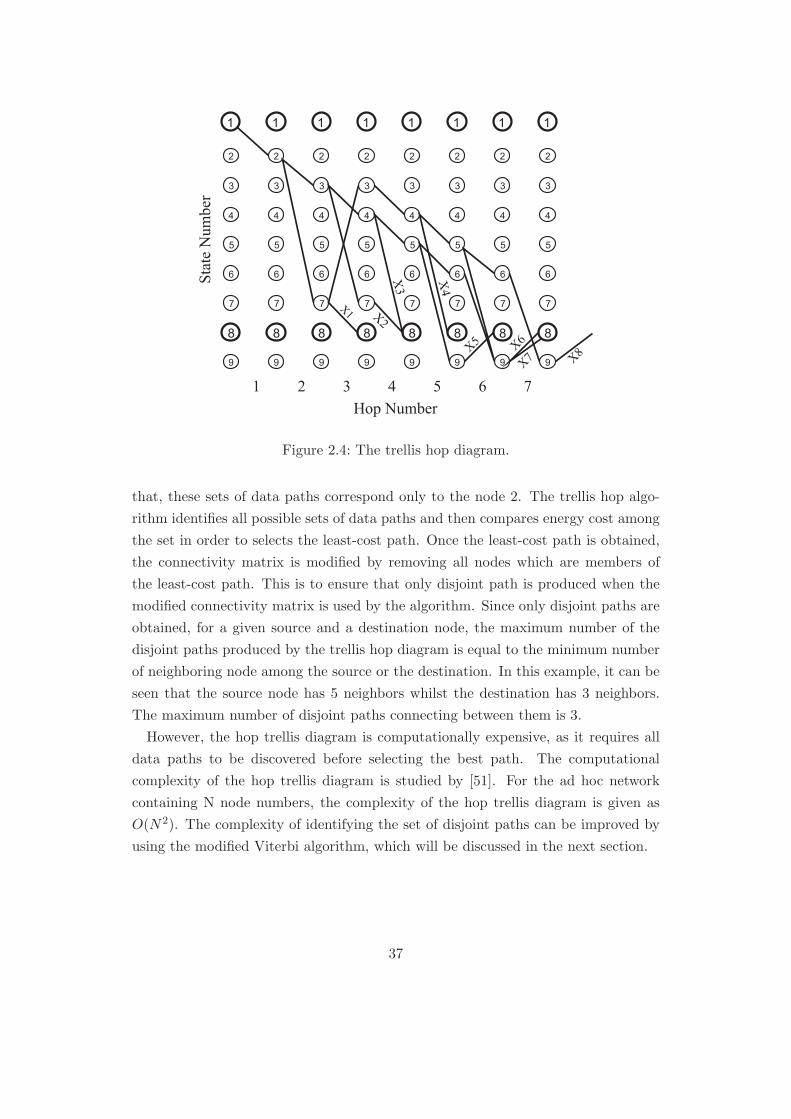
1

8

2

3

4

5

6

7

9

1

8

2

3

4

5

6

7

9

1

8

2

3

4

5

6

7

9

1

8

2

3

4

5

6

7

9

1

8

2

3

4

5

6

7

9

1

8

2

3

4

5

6

7

9

1

8

2

3

4

5

6

7

9

1

8

2

3

4

5

6

7

9

Sta

te N

um

ber

1 2 3 4 5 6 7

Hop Number

X1 X

2

X3

X4

X5 X

6

X7 X

8

Figure 2.4: The trellis hop diagram.

that, these sets of data paths correspond only to the node 2. The trellis hop algo-

rithm identifies all possible sets of data paths and then compares energy cost among

the set in order to selects the least-cost path. Once the least-cost path is obtained,

the connectivity matrix is modified by removing all nodes which are members of

the least-cost path. This is to ensure that only disjoint path is produced when the

modified connectivity matrix is used by the algorithm. Since only disjoint paths are

obtained, for a given source and a destination node, the maximum number of the

disjoint paths produced by the trellis hop diagram is equal to the minimum number

of neighboring node among the source or the destination. In this example, it can be

seen that the source node has 5 neighbors whilst the destination has 3 neighbors.

The maximum number of disjoint paths connecting between them is 3.

However, the hop trellis diagram is computationally expensive, as it requires all

data paths to be discovered before selecting the best path. The computational

complexity of the hop trellis diagram is studied by [51]. For the ad hoc network

containing N node numbers, the complexity of the hop trellis diagram is given as

O(N2). The complexity of identifying the set of disjoint paths can be improved by

using the modified Viterbi algorithm, which will be discussed in the next section.

37

The Modified Viterbi Algorithm

The modified Viterbi algorithm [27] is based on the hop trellis diagram but the least-

cost path selection algorithm and the path discovery algorithm is improved. Using

the modified Viterbi algorithm the cost metric is computed during path identifying

process. The total cost of uncompleted paths will be compared, if it is necessary,

and only the lowest cost path is selected and kept in the uncompleted routing table.

As a result, the number of uncompleted paths to be considered during the process

as well as the complexity are reduced.

The algorithm is operated similarly as the hop trellis diagram, but the cost is

calculated in each step. In a set of uncompleted path, if there are paths going

to the same node, the algorithm compares their cost. The higher cost path is then

removed from the table and the algorithm continuous at the next hop level with those

uncompleted paths remaining in the table. Once the algorithm is stop running, only

one least-cost path will be obtained and the algorithm then modifies the connectivity

matrix to be used in the next search. The algorithm is replicated just the same way

as the hop trellis done to identify all disjoint paths. Since the number of uncompleted

path can be reduced during each searching time, the computational complexity of

the modified Viterbi algorithm is reduced to O(N).

In order to examine the modified Viterbi algorithm, simulations on the 50 nodes

ad hoc network, given in Figure 2.1, has been set up. It is assumed that the max-

imum transmission range for each node is fixed at 200 metres and there are three

transmission techniques, the single code CDMA, the multi-code CDMA with the sin-

gle bit allocation and the multi-code CDMA with two-group bit allocation employed

in communications. For each transmission scheme operated at the physical layer,

the modified Viterbi algorithm is used to identify a set of disjoint paths connecting

between node 37 and node 3. Firstly, the single code CDMA code communication

with the modified Viterbi algorithm is run. The result is given in a Figure 2.5. It

can be observed from the Figure 2.5 that the single code CDMA with the modified

Viterbi algorithm obtains 5 disjoint paths. The path labeled by a blue line is the

first path discovered by the algorithm, which is the most least-cost path. The set of

the discovered paths consists of J1 = 37, 35, 46, 4, 3 , J2 = 37, 49, 47, 2, 3 , J3 =

37, 36, 45, 44, 3 , J4 = 37, 29, 48, 50, 5, 3 and J5 = 37, 31, 32, 33, 8, 7, 3. How-

ever, because data rates produced by the single code CDMA is very low, total

bit energy consumption of these paths are very high. As a result, when these

data paths are employed in data transmission, life time of each path is short.

38

J1J3

J2

J4J5

Sourcenode

Destinationnode

Figure 2.5: A set of disjoint paths produced by the modified Viterbi algorithm andthe single-code CDMA scheme.

The data path lifetime will be discussed in the next section. Next, the modi-

fied Viterbi algorithm incorporated with the multi-code CDMA with the single

group bit allocation is operated, which provide a set of disjoint path as shown

in the Figure 2.6 when the multi-code CDMA with the single group loading ap-

proach is employed, according to the standard of the HSDPA technique, each pair

of communication needs to have an SNR sufficiently high to operate transmis-

sions with the minimum bit rate on at least 5 channels. Otherwise, it is consid-

ered as no link between them. Therefore, the number of data links in Figure 2.6

is lower than in Figure 2.5, as all low SNR links are removed. It can be seen

that the multi-code CDMA with the single group bit allocation provides 3 disjoint

paths, which is J1 = 37, 49, 36, 32, 47, 4, 3 , J2 = 37, 35, 33, 50, 45, 44, 3 and J3 =

37, 30, 28, 29, 48, 46, 5, 3. Although the number of disjoint paths to be used in this

scheme is smaller than the single code communication, the total bit energy consump-

tion of each path is significantly lower. Finally, a set of disjoint paths given by the

modified Viterbi algorithm collaborating with the multi-code CDMA with the two-

group loading approach is shown in Figure 2.7. The approach utilizes transmission

energy effectively to improve the data rate. As a result, low SNR link is able to oper-

ate data transmission. There are 4 data paths given by the multi-code CDMA with

the two-group loading technique, where the total bit energy consumption of each

path is minimized. The data paths of the two-group loading approach comprises J1 =

39

J1

J2

J3

Sourcenode

Destinationnode

Figure 2.6: A set of disjoint paths produced by the modified Viterbi algorithm andthe multicode-code CDMA with the single-group bit allocation scheme.

37, 49, 36, 32, 47, 4, 3 , J2 = 37, 30, 28, 38, 42, 43, 2, 47 , J3 = 37, 35, 48, 45, 44, 3and the path J4 = 37, 23, 21, 20, 19, 18, 17, 15, 34, 8, 5, 3.

The multi-path routing communication is able to identify the set of the least-cost

disjoint paths for data transmission but those disjoint path discovered in the later

state are slower data rate paths, which consume more energy for transmitting the

same amount of data. The energy cost of each path is not identical so that allocating

data equally into all path causes the energy unequal energy consumption, which

reduce the network lifetime and energy efficiency. Therefore, to enhance energy

efficiency, energy consumption must be spread uniformly across the set of the disjoint

paths, which can be done by using the load balancing algorithm,demonstrated in

the next section.

2.2.4 Maximizing the Lifetime of the Networks

In this work, the network lifetime is defined as the period of time since the network is

deployed until some nodes in the network run out of energy, or it can be said that, for

the multi-path communication, the network lifetime is equal to the shortest lifetime

of the paths. The network lifetime is one of the factors to be used to indicate

how network consumes energy effectively, the energy efficiency. In conventional ad

hoc networks, the data packets are delivered over a single data path, known as the

best path, so that nodes constitute the data path exhaust energy quickly, rendering

40

J1

J2

J3

J4

Sourcenode

Destinationnode

Figure 2.7: A set of disjoint paths produced by the modified Viterbi algorithm andthe multicode-code CDMA with the two-group bit allocation scheme.

the short lifetime of the network. Therefore, having the multiple data paths in

transmission can enhance the network lifetime as energy consumption can be spread

over all paths. However, energy cost on each data path is not uniform so that it is

important to allocate data into each data path properly. Otherwise, system cannot

take advantage of the multi-path communication.

Now, giving M data bits to be transmitted over multiple data paths in a period

time of T second, the required transmission rate hence is given as M/T bits per

second. Assuming the M data bits are distributed to each data path z with a

number of bit denoted by mz, the data rate on path is given as mz/T , which satisfyMT =

∑Zz=1

mzT . The energy draining rate which show an amount of energy consumed

by path z in each second can be written as

Dz =Eb,zmz

T(2.29)

Giving an average transmission energy on the data path as Eini, the average lifetime

of the data path is formulated as

tl,z =Eini

Dz(2.30)

For the network using a multipath routing, the network lifetime can be determined

by using (2.30), as it is assumed to be equal to the lowest average path lifetime.

41

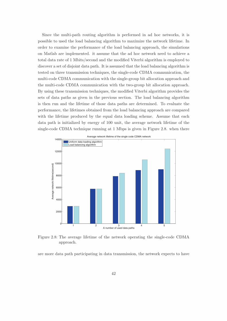
Since the multi-path routing algorithm is performed in ad hoc networks, it is

possible to used the load balancing algorithm to maximize the network lifetime. In

order to examine the performance of the load balancing approach, the simulations

on Matlab are implemented. it assume that the ad hoc network need to achieve a

total data rate of 1 Mbits/second and the modified Viterbi algorithm is employed to

discover a set of disjoint data path. It is assumed that the load balancing algorithm is

tested on three transmission techniques, the single-code CDMA communication, the

multi-code CDMA communication with the single-group bit allocation approach and

the multi-code CDMA communication with the two-group bit allocation approach.

By using these transmission techniques, the modified Viterbi algorithm provides the

sets of data paths as given in the previous section. The load balancing algorithm

is then run and the lifetime of those data paths are determined. To evaluate the

performance, the lifetimes obtained from the load balancing approach are compared

with the lifetime produced by the equal data loading scheme. Assume that each

data path is initialized by energy of 100 unit, the average network lifetime of the

single-code CDMA technique running at 1 Mbps is given in Figure 2.8. when there

Figure 2.8: The average lifetime of the network operating the single-code CDMAapproach.

are more data path participating in data transmission, the network expects to have

42

a longer lifetime, as the amount of data to be transmitted can be shared by each

data path. However, for the system using the single code CDMA communication, it

can be observed that the network lifetime is not improved as the number of paths

increases, if the data is allocated equally to all paths. This is because the paths

discovered later has a high total bit energy consumption and those paths consume

large energy even to carry small bits of data. As a result, the network lifetime of

the single code CDMA is not improved much for the equal data loading scheme. On

the other hand, the load balancing algorithm allocate amount of data accordingly,

which contributes to uniform energy consumption over all data path. The average

network lifetime therefore can increase proportionally to the number of data path.

The simulation results for the multi-code CDMA with the single group allocation

is demonstrated in the Figure 2.9. The multi-code CDMA with the single group

Figure 2.9: The average lifetime of the network operating the multi-code CDMAwith the single-group bit allocation approach.

bit allocation significantly enhances the total data rate and the network lifetime

compared with the single-code CDMA approach. It is noticeable here that the

uniform data allocation produces poor lifetime as more data paths are used, since

the data path 3 is very slow data path consume too much energy for transmitting

the same amount of data. The lifetime of the data path three is the shortest so that

it consider as the network lifetime. Finally, the network lifetime of the system using

the multi-code CDMA with the two-group bit allocation technique is presented in

Figure 2.10. It can be observed that further improvement of the lifetime is provided

by the two-group bit allocation, where the maximum lifetime increases by 20%

compared with the single group allocation. Moreover, the result also confirms that

43

Figure 2.10: The average lifetime of the network operating the multi-code CDMAwith the two-group bit allocation approach.

the load balancing algorithm is necessary for maximizing the network lifetime.

Having the multipath communication with the load balancing algorithm maxi-

mizes energy efficiency, but not the target end-to-end throughput. The effective

throughput actually depends on MAC protocols as it controls data traffic in net-

works. A carefully investigation on the MAC protocol is required in order to estimate

the end-to-end throughput correctly, which will be used to improve the end-to-end

throughput. In the next section, an analytical model for the MAC protocol is de-

scribed. The model provides the MAC’s service time indicates the time required to

complete one packet transmission. The service time is necessary parameter which is

employed in the end-to-end throughput enhancement.

2.3 The MAC Layer and the Service Time Calculation

In conventional ad hoc networks, MAC protocols control channel access on all nodes

and limit the amount of data that a node can transmit. The effective throughput

of an ad hoc network is given by (2.1), where L is length of data bits in the payload

of packets and T is the transmission duration allocated by a MAC protocol. The

time T is known as the MAC’s service time, which vary in each node in the network.

The service time depends on the network topology and data traffic, and it is also

associated with the physical data rate. Assuming that the ad hoc network employs

the multi-path routing to transmit M bits of data in a given time T second, the

target throughput of the ad hoc network is given as R = M/T bits/second. The

44

data M is spread over multiple paths such that R =∑Z

z=1mzT , where mz is data

allocated for path Jz for z = 1 , . . . , Z. For every node i and node l where i, l ∈ Jz,

the service time between the nodes is given as T i,l. The service times of each link in

the path Jz are different and the link with the maximum service time is known as a

bottleneck link, which limits the maximum throughput of the path Jz, as previously

stated in (2.2). The MAC protocol assembles packets from a given data before

transmission, and if the MAC protocol produces a packet length of Lz bits, The

maximum data rate given by the MAC protocol over the path Jz is written as

RMAC,z,MAX =Lz

maxi,l∈Jz

(T i,l

) (2.31)

where maxi,l∈Jz

(T i,l

)is the maximum service time of path Jz. In order to satisfy

the required throughput R, the optimum packet Lz must be determined such that

Lz

maxi,l∈Jz

(T i,l

) =mz

T(2.32)

It can be observed from (2.32) that the maximum service time is required in the

calculation. In this work, the link’s service time can be estimated by using the

Carvalho’s analytical model [30]. The model is proposed to calculate the service

time of ad hoc networks in which the MAC protocol corresponding to the IEEE

802.11 standard is performed. Moreover, it is able to calculate the service time

for the entire network regardless of the network topology. The Carvalho’s model is

described in the next section.

2.3.1 The Carvalho’s Service Time Model

The model is used to calculate the service times for saturated networks where all

nodes in the networks have packets ready to be transmitted and queue delay time

is not considered. The service time determined by the model is given as

T = TB + T s (2.33)

According to the IEEE 802.11 with Distributed Coordinate Function (DCF) MAC

protocol, TB is average time that node spend in a binary backoff state and TS is

time required to complete one packet transmission after the backoff period expire.

The binary backoff is a mechanism that the IEEE 802.11 DCF MAC protocol is

45

used to solve packet collision in the network. The backoff basically is a timer es-

tablished by the node encountering the packet collision or unsuccessful transmission

attempts. Once the backoff is set, the node is forced to be idle and remains in that

state until the backoff time is over. The backoff timer comprises multiple time slots,

where each time slot size is equal to an interval of time required by a node to detect

packet transmission performed by the others. The number of time slots for setting

up the backoff time is initialized by a random integer number running between 0

and w − 1, where w is called a contention window. The contention window begins

with wmin and it increases by a factor of 2 power every time the node detects more

unsuccessful transmission. The maximum number of the contention windows is de-

noted by wmax. During the backoff process, the backoff time is reduced only if the

node observes and finds that the communication channel is unoccupied for a period

longer than the period of Distributed Inter-Frame Time Slot (DIFs), and the node

is allowed to used the channel once the backoff timer is over, as it can be seen in the

Figure 2.11 In order to determine the average backoff time of each node, the model

Figure 2.11: DCF and the backoff time. [2]

takes correlations between the physical layer and the MAC layer into account. The

relationship between both layers is formed as a linear equation such that

τ = f(q) (2.34)

where τ and q represent a transmission scheduling rate and a successful transmission

probability respectively. The transmission scheduling rate τ a parameter of the MAC

protocol, which indicates the opportunity of transmitting packets given to each node

whilst the successful transmission probability q is a parameter of the physical layer

which denotes the successful rate once a packet is transmitted. The node with a

46

high successful transmission rate has a higher chance for data transmissions, as it

can be seen in (2.34). Since the network is saturated and all nodes are allowed to

send packets simultaneously, there may be packet collision occurring at receivers.

However, in the case that receivers perceive a low level of interference those collided

packets can be successfully received, as they can be recovered by an error correction

mechanism. Consequently, the successful transmission probability q of each node

depends on the interference level, or the received SNIR. Since the ad hoc network

is saturated, queue delay time is excluded and (2.34) can be rewritten in a vector

notation to represent the scheduling rate of all N nodes in the network as follows

τ = aq (2.35)

where τ = [τ1 τ2 , . . . , τN ]T and q = [q1 q2 , . . . , qN ]T . the constant a is a parameter

of the MAC protocol which can be calculated from the contention window as

a =2wmin

(wmin + 1)2(2.36)

The probability q is associated with two parameters, the bit error rate of received

packets and the interference appearing at the point of interest. The bit error rate is

calculated both in the forward direction, when a data packet is sent to the receiver,

and in the reverse direction, when the receiver sends an acknowledge packet to the

transmitter. The interference estimation considers only node in the carrier sensing

area of the transmitter and the receiver. The q vector is formulated as

q = (I + Φ)−1π (2.37)

where I is a N×N dimensional identity matrix for a network with N nodes and π =

[π1 π2 , . . . , πi , . . . , πN ]T is a vector comprising the total bit error rate encountered

by node i for i = 1 , . . . , N whilst Φ is called an interference matrix.

The total bit error rate πi is calculated as a function of the conditional probability

of successful frame reception as given in the follows

πi = f(cri0)f(cir0) (2.38)

the conditional probability f(cri0) is estimated from the bit error rate determined at

47

the SINR level of γ, Pb(γ), and a transmitted packet size K such that

f(cri0) = [1 − Pb(γ(cri0))]K (2.39)

the f(cri0) represents the transmission of data in the forward direction and K is

the size of the transmitted packet given in bits. Similarly, the f(cir0) is used in the

reverse direction where the packet to be transmitted is the acknowledgment packet

instead of the transmission data packet. The interference matrix has a dimension

N × N which describes how interference exists between the nodes in the network.

The interference matrix is given as

Φ =

0 Φ12 Φ13 · · · Φ1N

Φ21 0 Φ23 · · · Φ1N

Φ31 Φ32 0 · · · Φ32

......

.... . .

...

ΦN1 ΦN2 ΦN3 · · · 0

(2.40)

where each element in the matrix is

Φil =

aπi, if l ∈ Vi ∪ Vri

0, if l /∈ Vi ∪ Vri

(2.41)

where Vi is the set of nodes staying in the carrier sensing area of node i and Vri is

a set of nodes staying in the carrier sensing domain of the promise receivers of node

i. The parameter a can be obtained from (2.36). Once the successful transmission

vector q is calculated, the transmission scheduling rate matrix can be determined

by using (2.35).

The Carvalho’s model assumes that only three events are encountered by nodes

i while it is in the backoff state. The events consist of successful transmission,

idle and collision, which can be described by a channel state probability vector

pi

=[pii p

ic p

is

]Twhere pii, p

ic and pis stand for an idle channel probability, a collision

channel probability and a successful channel probability. The channel state prob-

ability vector exists, if other nodes are transmitting in the carries sensing area of

the node i. Hence, to calculate the channel state probability pi

, the probability of

transmission will need to be calculated. Giving Ri as a set of nodes appearing in

the carrier sensing area of node i, the possibility that the nodes in this set transmit

48

data while node i is in a backoff state is written as

pitr = 1 −∏

j /∈Ri

(1 − τj) (2.42)

where τ is obtained from (2.35). once the data transmissions happen within carrier

sensing range of node i, the probability that these transmissions are done successfully

is obtained as

pisuc =

∑k/∈Ri

qkτk

pitr(2.43)

Using the pitr and pisuc, the idle channel probability, the collision channel probability

and the successful channel probability are formulated as

pii = 1 − pitr

pic = pitr(1 − pisuc)

pis = pitrpisuc

(2.44)

The channel state probability is employed to estimate the average backoff time of

node i, which is given as

TB =α(wminβ − 1)

2q+

1 − q

qtc (2.45)

where

α =q − 2m(1 − q)m+1

1 − 2(1 − q)(2.46)

where m is a standard power determined from the maximum contention window

size such that wmax = 2mwmin. The parameter α denotes the average time that the

node spend in each channel state, which is calculated as a function of the channel

state probability, as follows

α = σi + tcpc + tsps (2.47)

For node i, each channel state probability is obtained from the vector pi

=[pii p

ic p

is

]T.

The time coefficient σ is an interval of the backoff time slot while tc and ts are an

average time that the system expects to encounter data collisions and an average

time of completing packet transmissions respectively. The ts includes all periods of

time for processing one packet transmission by a four-step handshake mechanism

(RTS-CTS-DATA-ACK) defined in the IEEE 802.11 MAC protocol. The four-step

49

handshake protocol is shown in the Figure 2.12

Figure 2.12: The four-step handshake protocol. [2]

To obtain tc, the system assumes that the collisions happen only in during the

overhead packet transmission. This is because, if the overhead packet exchanging is

completed, nodes surrounding the communication pair are forced to be idle by the

protocol, which cannot interrupt the data transmission. Hence, the tc is given as

tc = tRTS + tDIFs + δ (2.48)

where tRTS ,tDIFs and δ is the time required to complete transmission of the RTS

packet, the interval of DCF interframe time space and the propagation dalay. In

this work, it is assumed that all control packets are transmitted with a constant

data rate of 1 Mbps. The propagation delay δ is very small compared with other

delay time so that it is assumed to be equal in all links and the approximate value

will be assigned. The successful tranmsission time ts is obtained as

ts = A +L

rdata(2.49)

where A = tRTS+tDIFs+3tSIFs+4δ+tMACheader+tCTS+tACK . tCTS and tACK are

time required to complete transmission of the CTS packet and the acknowledgment

packet respectively. tSIFs is the short interframe time space specified by the MAC

DCF protocol. It also assumes that all header packets are transmiitted with the

constant data rate of 1 Mbps whilst a data rate rdata, given in bits/sec, is used

only when transmitting the data payload L.For a given node i and node l, the data

rate ri,ldata is determined as ri,ldata = ri,l/(NPGTs). Each time parameters used by

50

(2.48) and (2.49) are taken from to standard values given by the IEEE 802.11 MAC

protocol. These parameters are shown in the table 2.2. The Carvalho’s model can

Table 2.2: The IEEE 802.11DCF MAC protocol’s parameters

wmin 32

wmax 1024

MACheader 34 bytes

tRTS 44 × 8 µS

tCTS 38 × 8 µS

tACK 38 × 8 µS

σ 20 µS

tSIFs 10 µS

tDIFs 50 µS

δ 1 µS

be used to estimate the service times for saturated networks, where all nodes are

transmitting data packets. However, for the network we are interested in packet

transmission are operated only by nodes which are members of a data path. As

there is some discrepancy, applying the Carvalho’s model directly on the network

may contribute to inaccurate results. Therefore, it is necessary to examine the

accuracy of the Carvalho’s model when it is used in the given network.

For the testing, the Carvalho’s model is applied for services times calculation of

each link over a data path, which is constructed on the 50 node ad hoc network given

in the Figure 2.1. The results produced by the Carvalho’s model are then compared

with the sets of results obtained from the network simulator NS-2 [32], which is run

under the same condition. The data paths to be examined for the link service times

are given as J1 = 37, 49, 36, 32, 47, 4, 3 and J2 = 37, 30, 28, 38, 42, 43, 2, 3. The

results are illustrated by the Figure 2.13 and the Figure 2.14.

It can be observed from Figures 2.15 and Figure 2.16 that the service times cal-

culated by the Carvalho’s model are exceptionally high compared with the service

time obtained from the NS-2. Since the NS-2 is known as a tool to give practical

results, it means using Carvalho’s model may produce another set of results which

is different from the practical. This is because the Carvalho’s model considers all

nodes in the network for the calculation. As a result, the interference domain and

the number of activated nodes in the carrier sensing range of each node are large,

which contribute to very high service time in each communication link. On the other

hand, in the NS-2 simulation, all nodes are idle except the nodes belonging to the

51

Figure 2.13: Data path J1.

Figure 2.14: Data path J2.

data path. Therefore, the number of nodes that can interrupt the communication

is minimized, which results in the low link services times. As it can be observed

from the examination, the Carvalho’s model needs to be modified before applying

to calculate link service times in ad hoc networks. Otherwise, inaccurate service

times may be obtained.

52

Figure 2.15: The link service time of data path J1.

2.3.2 The Modification of the Carvalhos Service Time Model

From the NS-2 simulation, two reasons causing discrepancy in the service time

between the NS-2 simulation and the Carvalhos model has been observed. Firstly,

the carvalhos model takes all nodes in the network into consideration in order to

calculate the service time. Consequently, the service time in each data link is very

high, since the number of node create data collision is large. On the other hand,

in the NS-2 simulator, once data path is established, only nodes which are the

member of the data path are activated, and data collision only caused by these

nodes. Therefore, the number of node making the collision in the NS-2 is much

lower than in the Carvalhos model.

Secondly, it has been observed in the NS-2 that the packet collision always hap-

pen at the receiver during the RTS transmission. Once the transmitter send the

RTS packet to the receiver and the receiver is waiting to reply by sending the CTS

packet, the receiver sometime encounters another transmission caused by neighbour-

ing nodes. These neighbouring nodes are known as interferer which can interrupt

the data transmission, as they are not in the range of the transmitter and cannot

hear the RTS transmission produced by the transmitter. In the NS-2, the interferes

appear only in the carrier sensing range of the receiver as shown by the Figure 2.17.

Alternatively, in the Carvalhos model the interferer exists in both transmitter and

receiver carrier sensing distance, since it considers data transmission in both forward

53

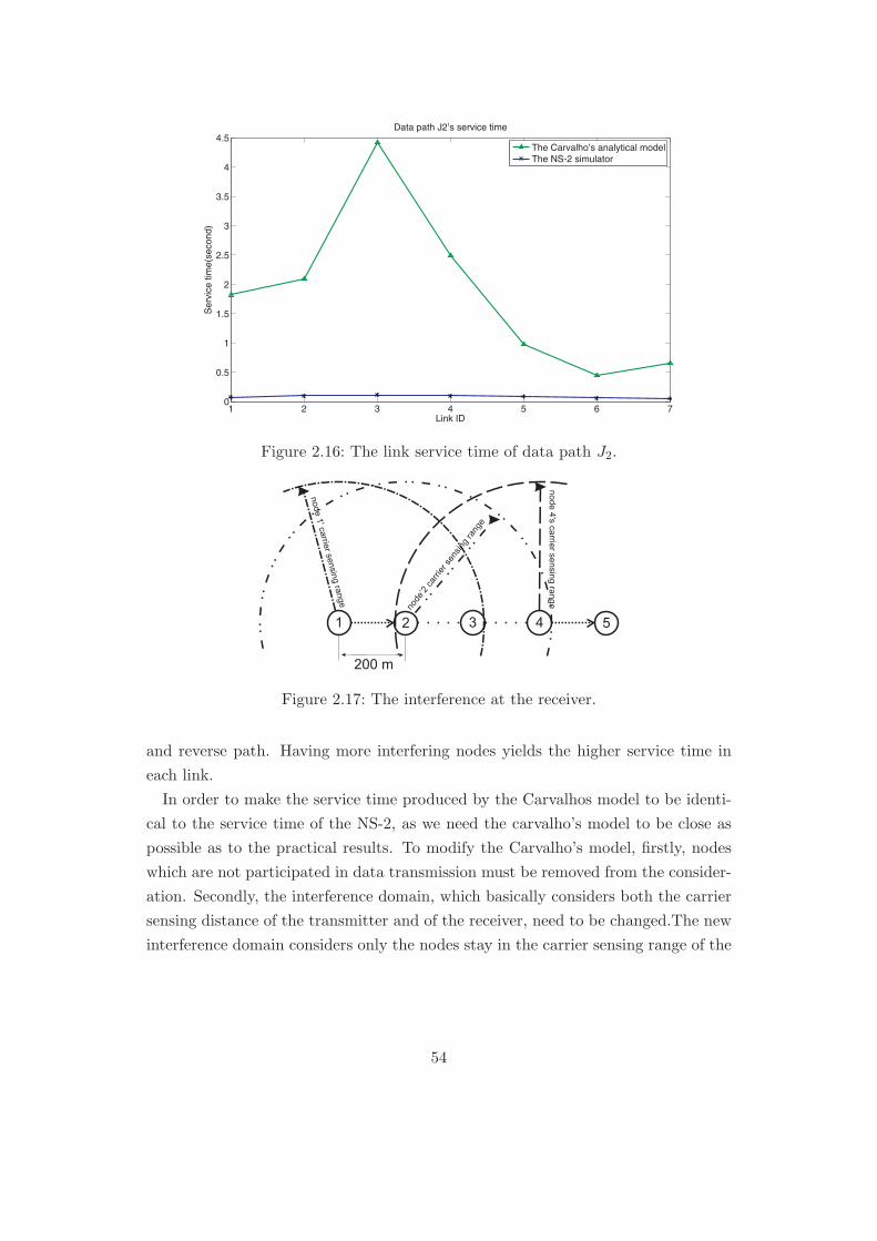
Figure 2.16: The link service time of data path J2.

node

1' c

arrie

r sensin

gra

nge

node

’2ca

rrie

rse

nsin

gra

nge

node 4

's c

arrie

r sensin

g ra

nge

Figure 2.17: The interference at the receiver.

and reverse path. Having more interfering nodes yields the higher service time in

each link.

In order to make the service time produced by the Carvalhos model to be identi-

cal to the service time of the NS-2, as we need the carvalho’s model to be close as

possible as to the practical results. To modify the Carvalho’s model, firstly, nodes

which are not participated in data transmission must be removed from the consider-

ation. Secondly, the interference domain, which basically considers both the carrier

sensing distance of the transmitter and of the receiver, need to be changed.The new

interference domain considers only the nodes stay in the carrier sensing range of the

54

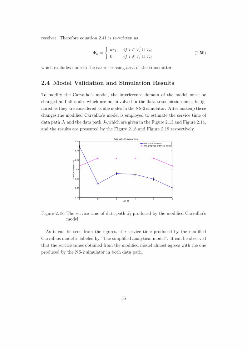
receiver. Therefore equation 2.41 is re-written as

Φil =

aπi, if l ∈ V

′

i ∪ Vri

0, if l /∈ V′

i ∪ Vri

(2.50)

which excludes node in the carrier sensing area of the transmitter.

2.4 Model Validation and Simulation Results

To modify the Carvalho’s model, the interference domain of the model must be

changed and all nodes which are not involved in the data transmission must be ig-

nored,as they are considered as idle nodes in the NS-2 simulator. After makeup these

changes,the modified Carvalho’s model is employed to estimate the service time of

data path J1 and the data path J2,which are given in the Figure 2.13 and Figure 2.14,

and the results are presented by the Figure 2.18 and Figure 2.19 respectively.

1 2 3 4 5 60.04

0.06

0.08

0.1

0.12

0.14

0.16

Link ID

Serv

ice tim

e(s

econd)

Data path J1’s service time

The NS−2 simulator

The simplified analytical model

Figure 2.18: The service time of data path J1 produced by the modified Carvalho’smodel.

As it can be seen from the figures, the service time produced by the modified

Carvalhos model is labeled by ”The simplified analytical model”. It can be observed

that the service times obtained from the modified model almost agrees with the one

produced by the NS-2 simulator in both data path.

55

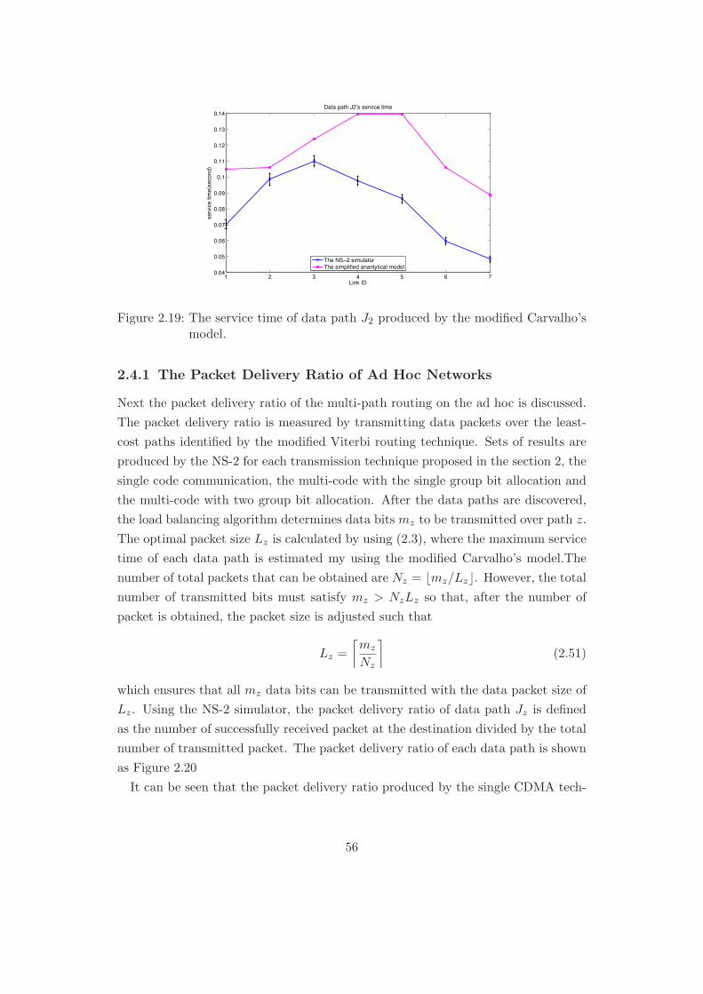
1 2 3 4 5 6 70.04

0.05

0.06

0.07

0.08

0.09

0.1

0.11

0.12

0.13

0.14

Link ID

serv

ice tim

e(s

econd)

Data path J2’s service time

The NS−2 simulator

The simplified ananlytical model

Figure 2.19: The service time of data path J2 produced by the modified Carvalho’smodel.

2.4.1 The Packet Delivery Ratio of Ad Hoc Networks

Next the packet delivery ratio of the multi-path routing on the ad hoc is discussed.

The packet delivery ratio is measured by transmitting data packets over the least-

cost paths identified by the modified Viterbi routing technique. Sets of results are

produced by the NS-2 for each transmission technique proposed in the section 2, the

single code communication, the multi-code with the single group bit allocation and

the multi-code with two group bit allocation. After the data paths are discovered,

the load balancing algorithm determines data bits mz to be transmitted over path z.

The optimal packet size Lz is calculated by using (2.3), where the maximum service

time of each data path is estimated my using the modified Carvalho’s model.The

number of total packets that can be obtained are Nz = ⌊mz/Lz⌋. However, the total

number of transmitted bits must satisfy mz > NzLz so that, after the number of

packet is obtained, the packet size is adjusted such that

Lz =

⌈mz

Nz

⌉(2.51)

which ensures that all mz data bits can be transmitted with the data packet size of

Lz. Using the NS-2 simulator, the packet delivery ratio of data path Jz is defined

as the number of successfully received packet at the destination divided by the total

number of transmitted packet. The packet delivery ratio of each data path is shown

as Figure 2.20

It can be seen that the packet delivery ratio produced by the single CDMA tech-

56

1 2 3 4 50

0.2

0.4

0.6

0.8

1

Routing path

Packet

deliv

ery

ratio

Multi code with two group allocation

Multi code with single group allocation

Single code

Figure 2.20: The delivery ratio observation.

nique is much lower than the ratio produced by the multi-code CDMA approach.

The delivery ratio of the multi-code CDMA with single-group approach is identical

to the ratio produced by the multi-code CDMA with two-group technique. However,

with the two-group resource allocation technique, there is one more data path to be

used so that the energy consumption per path is lower, which contribute to higher

lifetime as well as energy efficiency.

2.5 Conclusions

In this chapter, the end-to-end performance of ad hoc networks is enhanced. The

improvement of the ad hoc network has been done by cross-layer optimization which

includes optimizing the physical layer, routing layer as well as the MAC layer. At the

physical layer the multi-code CDMA with the two group resource allocation tech-

nique is implemented. The two group technique significantly improves the physical

data rate and minimize the residual energy. The energy efficiency is provided by

the routing layer, where a multi-path routing technique is employed. The multi-

path routing technique uses a bit-energy consumption as cost matrices to identify

a set of disjoint paths. The disjoint path with the minimum bit-energy consump-

tion is selected for transmission.This will ensure only the least-cost data paths are

57

employed in order to minimize energy consumption. The load balancing algorithm

is then utilized to distribute data to be transmitted equally to all paths. The load

balancing algorithm spread the energy consumption uniformly across the network.

As a result, the network lifetime as well as energy efficiency is improved when more

disjoint data paths participate in data transmission. In addition to the routing layer,

to improve the complexity for determining the set of the disjoint path,the modified

Viterbi algorithm is exploited instead of the trellis hop algorithm. However, the

actual end-to-end throughput is controlled by the MAC layer so that, to achieve the

target end-to-end throughput required by a user, a packet lenght optimiation on the

MAC layer need to be done. To calculate the optimal packet size, the maximum

service time of the data path is required, which can be estimated by using Carvalho’s

service time model. However, examining the Carvalho’s model found that the model

is unable to provide accurate service time values, when applying on the interested

network.

The main contribution of the chapter is examining and modifying the Carvalho’s

service time model. To examine the model, the set of result produced by the NS-

2 is used as a reference. The NS-2 is set to simulate the interested network for

determining the serveice times, which are compared to another set of the service

time calculated by using the Carvalho’s model. It is found that the results obtained

from the Carvalho’s model are much higher than the results given by the NS-2.

Therefore, to make the Carvalho’s model to be more accurate, the model need to

be modified. After adjusting, the Carvalho’s model is used to estimate the service

time, which will be used further to identify the optimum packet size. The result has

shown in the section 5.

For the further performance enhancement of the wireless network, it can be done

by improving the physical data rate. As shown by (2.25), the bit energy consumption

is inversely proportional to the physical data rate so that the bit energy consump-

tion can be reduced by increasing the data rate. Since the bit energy consumption

is reduced, the network consume energy more effectively, which results the higher

energy efficiency. Enhancing the data rate not only improves the energy efficiency

but the end-to-end throughput of the system as well. Since the end-to-end through-

put depend on the maximum service time of the data path and the service time is in

inversely proportion to the data rate, increasing the data rate therefore improve the

end-to-end throughput. In the next chapter, an enhancement of the data rate using

the MIMO-HSDPA technique will be demonstrated. The MIMO communication

technique specified by 3GPP basically can double the data rate of the system. How-

58

ever, when data rate increase, the system encounters the frequency selective channel

instead of a flat fading channel. The next chapter also performs a method to deal

with the frequency selective channel together with resource allocation technique,

which optimize the performance of the of the MIMO-HSDPA system.

59

3 Resource Allocations and

Performance Evaluations on the

MIMO-HSDPA system

3.1 Introduction

In the Chapter 3, the energy efficiency and the throughput of ad hoc networks has

been investigated. Energy efficiency can be improved by using the load balancing

algorithm collaborating with the multipath routing approach, which uses a set of

the minimum energy consumption paths. Improvement of energy efficiency is de-

termined by the network lifetime and it has been demonstrated that the network

lifetime is extended when the schemes are implemented. Careful analysis found that

the critical parameter of ad hoc networks is actually a physical data rate. As you

can see from the multipath routing selection algorithm, consuming the same amount

of energy, the faster path can deliver more data. Therefore, using the faster path

results in the improvement of energy efficiency. Not only the energy efficiency which

is depended on the physical data rate, the end-to-end throughput as well.

The end-to-end throughput is inversely proportional to the maximum service time

in a data path, which is the parameter of the MAC layer, so that the end-to-end

throughput increases, if the maximum service time is reduced. It was shown in the

analysis of service time model of the MAC protocol that the service time inversely

proportional to the physical data rate. Hence, increasing the data rate reduces the

maximum service time and enhances the end-to-end throughput.

The previous chapter showed how to improve the physical data rate by using HS-

DPA with the two-group bit loading approach, where the system is operated on flat

fading channel.In this chapter, the further improvement of the data rate by utilizing

a MIMO transmission technique will be discussed. This will show that the MIMO

approach can significantly boost the physical data rates when collaborating with

resource allocation techniques. However, when the data rate increases, the commu-

60

nication channel might be changed from a flat fading channel to a frequency selective

channel, which causes inter-symbol-interference at the received signal. This chapter

will demonstrate an interference cancellation technique which is used to deal with

the frequency selective channel.The interference cancellation approach is utilized

in collaboration with the resource allocation technique, Equal-Energy-Equal-SNR

approach and Equal-Energy-Equal-Rate (EEER)approach, [53] such that the per-

formance of the MIMO-HSDPA system is substantially improved. The performance

of the proposed technique is evaluated by the simulation on a frequency selective

channel, which is represented by more sophisticated channel model.

In order to confirm the effectiveness of the proposed algorithm, examining the

technique on a test bed system has been set up. The test bed system has been build

base on software defined radio based LabVIEW-FPGA system, which is capable of

testing ultra-broadband transmission systems such as 3G or 4G systems. The test

bed system incorporates particular signal processing techniques so that no external

signal sources are required for the synchronization of the transmitter and the receiver

when operating the signal transmission. The detail of MIMO-HSDPA and the test

bed system is going to be discussed later. The detail of how to construct the test

bed system can be found in the appendix I.

3.2 Related Works

For improving downlink data rates of 3rd generation (3G) networks, the third gen-

eration partnership project (3GPP) introduced a high speed downlink packet access

(HSDPA) approach in release 5 [4]. In HSDPA systems, the data rate is signifi-

cantly improved by using an adaptive modulation and coding scheme including a

fast link schedule algorithm. The transmitter specifies the modulation and coding

scheme to a particular user based on channel information sent back from that user.

To provide the higher data rate, the use of a Multiple Input and Multiple Output

(MIMO) technique, where multiple antennas are used by transmitters or receivers,

was introduced in 3GPP release 7 [9]. In this release, 2 x 2 MIMO transmission

scheme called the Dual Stream Transmit Diversity (D-TxAA) is incorporated into

the HSDPA system specification, the system hence is able to transmit up two data

streams to users, which theoretically doubles the capacity of the system. Although

the MIMO-HSDPA techniques provide a considerable improvement for the system

but, in practice, the performance of the MIMO system still need to be examined.

Study conducted by [5] has been found that the capacity of MIMO-HSDPA is less

61

than the upper bound when the system is operated in practical systems. The paper

reviewed several reasons degrading the performance, which mainly are Inter-Symbol-

Interference (ISI) in the system and inefficiency of resource utilization.

Communication channels might be corrupted by multipath fading which causes

the channels to be a frequency selective channel, which distorts a signal. Once a

sequence of symbols is transmitted over the frequency selective channel, the sym-

bols might be spread in time and to the adjacent symbols, and this is known as

ISI which degrade the quality of received signals. Basically, both linear and non-

linear equalizer can be used to eliminate the ISI. The linear equalizer such as a

Zero-Forcing (ZF) equalizer is simply constructed by the inversion of the frequency

selective channel, which is modeled as a linear time invariant filter. However, the ZF

equalizer potentially leads to enhancement of noise power levels as it is not taken sys-

tem noise into consideration [54]. Alternatively, the Minimum-Mean-Square-Error

(MMSE) equalizer can be employed instead of the ZF equalizer, since it provides

the better performance in ISI and noise suppression. Comparing between the ZF

and the MMSE equalizers demonstrates that the MMSE equalizer is only slightly

complicated in analysis. The use of the MMSE equalizer can be found in [55, 56].

In [55], the MMSE equalizer was performed in marco-femto cell networks where

the MIMO transmission is operated and it confirms the effectiveness of the MMSE

equalizer. Study in [56] applied the MMSE equalizer on the system where uncertain

channel feedback information appears. But using only the MMSE equalizer might

not be effective as suggested by [5], which measures the throughput on two different

channel profiles, a short delay spread channel and a long delay spread channel. The

results showed that the long delay spread channel contributes to the higher lever of

the multipath fading and the subsequent interference which causes more throughput

loss.

For further improvement in the receiver, it is feasible to incorporate non-linear re-

ceiving techniques such as Successive Interference Cancellation (SIC) into the struc-

ture of the receiver. The SIC approach decodes and removes out the strong signal,

which is a potential interferer. As a result, the interference level is reduced, when

attempting to extract the desired signal. For example, the used of interference can-

cellation can be found in [57]. Work [57] attempted to improve the capacity of

radio down-links by using the MMSE-SIC receiver, and it demonstrated that the

MMSE-SIC receiver provides the better performance. Once the MMSE-SIC receiver

is exploited, the computational complexity is concerned, because the receiver needs

to run intensive computation in order to search for the coefficient matrix of the

62

equalizer. The computation includes the inversion of a channel covariance matrix

whose dimension is scaled the number of spreading sequence, the number of used

antenna as well as the number of resolvable path in the multipath fading channel.

For MIMO-HSDPA systems, the channel information is update for every 2 milli-

seconds according to the specification so that the computational cost is obviously

very high. In order to reduce the computational complexity, [58] proposed SIC based

matrix inversion method which minimizes the number of the matrix inversion when

calculating the MMSE linear de-spreading filter coefficients for multi-code HSDPA

systems. This approach can be applied on the MIMO-HSDPA as well.

Apart from optimizing receiver structures by using the MMSE-SIC approach, ef-

fective resource allocation algorithms are also required, in order to enhance the

capacity of MIMO-HSDPA systems. Since wireless resources are limited and shared

among users, allocating resource need to be done properly for maximizing the per-

formance. The optimization of the capacity might be achieved by using the famous

iterative water filling algorithm as described by [59]. In this work, the linear water-

filling algorithm is employed to solve capacity maximization problems in cognitive

radio systems, where interference and a power budget are limited. Work [60] per-

formed the water-filling algorithm on MIMO broadcasting systems to achieve energy

efficiency. Work [61] maximizes downlink throughput of CDMA systems by select-

ing the best group of uses to operate transmission. This problem is considered as

a scheduling problem which is done after power and spreading codes are properly

allocated. A dual formulation was exploited in this work as systems cost function

is constrained by the number of used codes and available transmission power. The

problem is formulated as a constrained optimization and Lagrangian method is pro-

posed to determine the solution. However, these works consider only a continuous

bit rate, which is impractical.

To make realistic systems, a discrete bit rate must be included in the problem. The

discrete bit loading has been studied by [62] and [63]. A rate maximization problem

and a margin maximization problem in multi-carriers systems were investigated

in [62], which also obtained the optimal solution by using the water-filling algorithm.

In addition to work [62], a discrete-bit loading problem was examined as well and

the modified water-filling algorithm was proposed to provide the solution. In [63],

a rate maximization including an optimal power allocation problem for MIMO with

MMSE-SIC receivers was formulated. The systems have considered a set of available

discrete- bit for power allocation. To maximize sum-rate, the maximum sum-rate

and the minimum required transmit power are determined. After that, the transmit

63

antenna set which satisfy those rate and power is selected to run transmission. The

proposed scheme also offers a good trade-off between the computational complexity

and information feedback rates.

Not only maximizing the performance of the MIMO-HSDPA system, the compu-

tational cost of resource allocation algorithm must be minimized in order to keep the

algorithm to be realistic. Although the water filling algorithm provides the optimal

solution for allocating resources, it is computationally expensive. The complexity of

the algorithm exponentially increase with as the number of users grows. In partic-

ular, the computational cost of the water filling algorithm might be exceptionally

high when consider discrete-bit allocation approach. To simplify and optimize re-

source allocation in MIMO-HSDPA systems, work [53] proposed resource allocation

algorithms based-on system values approach. The system values are parameters as-

sociated with the SNR at the output of de-spreading filters. For a MIMO-HSDPA

system using signature sequence for spreading data to be transmitted, the system

values for each spreading sequence can be calculated and they relate to a trans-

mission channel. The system values approach [58] is used to select the spreading

sequence creating high-gain coded channels. As a result, transmission energy can be

used more effectively to increase the total rate. For the rate allocation, the system

values approach is able to determine discrete data rates to be transmitted without

energy calculation, yielding reduction in computational cost. The total data rate

determined the system values approach is close to the maximum capacity of a given

channel.

Two resource allocation techniques are proposed to be used with the system values.

The first one is called the Equal-Energy-Equal-Rate (EEER) allocation. Using the

EEER approach, transmission energy is allocated equally into all code-channels,

which is similar to the standard MIMO-HSDPA, and all the channels are loaded by

the same data rate, which is estimated from the minimum system value. Another

loading scheme is known as the Equal-Energy-Equal-SNR (EEES) approach. The

EEES basically determine data rate to be allocated into each channel by using the

mean system value approach, and run iterative calculation to determine the amount

of energy which satisfy the data rate and produces identical received SNRs in all

channels. Since the iterative calculation is employed in the EEES approach, the

computational cost is higher than the EEER approach but it is able to achieve

the total rate which is very close to the system value upper bound. To confirm

the performance of the EEER and EEES approaches, experiments on a real system

have been undertaken. The test bed to run the experiments has been built on the

64

LabVIEW-PXIe systems provided by National Instrument (NI). The system is based

on the LabVIEW platform and work with channel emulator software, which is used

to generate various wireless multipath channels. The complete test bed system is

capable of supporting very high data rate processing, which is suitable for building

a test system for wideband communications such as HSDPA and LTE systems. The

LabVIEW-PXIe system was used to collect data for the chapter.

In order to evaluate the performance of algorithms, MIMO test bed systems are

required. At this moment, test bed systems are mainly developed on software radio

architecture, which is known as the Software Defined Radio (SDR) [64, 65]. The

SDR platform allows to define physical layer functions on a software and implement

by using the combination of electronics technologies such as a general-purpose pro-

grammable processing unit, analog-digital-analog (A/D/A) converter.It can be said

that all RF components and the baseband processes are converted as configurable

digital forms or it is the digit configurable radio (DCR).It is now being employed

widely to construct testbed systems for various applications. For example, a test bed

system for cognitive radio can be found in [66, 67]. For the RFID test bed system,

it is constructed in [68] and the test bed system for cellular networks is conducted

by [69, 70]. In work [66, 67], a survey on current technology of the SDR platform

has been demonstrated. [66] dedicated for identifying hardware which is suitable for

the cognitive radio systems. Many of hardware were examined in term of energy

consumptions, flexibility and computing ability. Similarly, in work [67] analyst the

hardware to be used for the test bed system of a cognitive radio and also discussed

about some of software available in the market. [67] demonstrated the SDR which

build on Matlab/Simulink and Universal-Software-Radio-Peripheral (USRP) [71] de-

vices. The USRP devices are selected to be used in the work [67], because they are

low-cost whilst the performance is acceptable when comparing with others. Actu-

ally, the USRP is a favorite device for the hardware platform of the SDR system and

it is also employed by [68] to construct a test bed for RFID systems. The SDR plat-

form for testing LTE cellular networks was proposed by [69]. The work developed

a baseband board which supports 4 x 4 MIMO-LTE transmission, requiring up to

48 Gbps data transfer rate in real-time. Another example of the test bed system is

conducted by [72,73]. This work used sophisticated hardware to build a system,the

Vienna MIMO testbed, for examining the performance of MIMO-HSDPA system.

This system uses Matlab and C language to implement data processing and generate

a signal vector to be transmitted.

Basically, Matlab can be used as a SDR software platform as it is capable of com-

65

puting intensively and it also provides communication toolboxes, which are ready to

operate signal processing. However, the run-time of the Matlab is not good enough

to perform real-time operation so that using Matlab as the SDR is effective only in

an off-line mode. Alternatively, GNU Radio [74], which is another famous software

platform for the SDR system, can be used instead of Matlab. The GNU radio is an

open-source software which is based on Linux operating system. The GNU radio

also provides a set of signal processing toolboxes to be used and it is compatible

with low-cost radio font-ends such as the USRP. However, the major drawback of

the GNU radio is that it is unable to do intensive computation. Moreover, using

the GNU radio requires expertise in the Linux operating system and developing a

new tool box set of the GNU radio is difficult, since it requires knowledge of Python

programming language as well as C programming. Recently, National Instrument

become a partner with the ETTUS research group, who produce the USRP de-

vice, and proposed LabVIEW to collaborate with the USRP for making the SDR

platform. The LabVIEW basically is comparable to Matlab but it use graphical-

based programming rather than text-based mode. LabVIEW is originally made for

monitoring and control systems so that they have ability for operating in real-time

mode. LabVIEW therefore is interesting software for making the SDR and test bed

systems. The use of LabVIEW-USRP test bed system can be found in [68, 75, 76].

Challenges and problems in building a MIMO test bed system were reviewed

by [77]. Generally, hardware and software available on market majority are unable to

satisfy the requirements for making the systems. For the hardware, they have limited

bandwidths and slow data transfer rates and, when they are used to make the test

bed system, they will encounter a synchronization problem between the transmitter

and the receiver. For the software, they have a limitation problem that make them

cannot be modified or it cost a lot of money for the modification, as licenses and

additional modules are required. The software also faces compatibility problems

which make them work only with particular hardware. In addition to the problem,

the documentation and the manual for the systems are poor, which make difficulty

in operations. Work [78] conducted an overview of the test bed technology. [78]

classifies hardware systems into three group, systems for demonstrating, systems

for prototypes and system for test bed which is the focus of the paper. The work

discussed about basic component in test bed systems and provided the comparison

between the systems from different manufacturers. Some of problem of the test beds

system was discussed in this work, which are lacking of tunable RF-front ends and

the methodologies for real-time implementations.

66

Apart from optimal resource allocation for MIMO-HSDPA systems, this chapter

also focus on building a test bed system in order to evaluate the performance on the

proposed techniques. The challenge in building the test bed system firstly is how

to synchronize the transmitter and a receiver without external clock signal. For the

best of our knowledge all of the test bed systems in the literature review require

the external signal source for synchronization propose. However, a precise external

signal source is expensive and is not available to our system. Therefore, we need to

do the synchronization base on a signal processing method. Secondary, the minor

problem of the test base system is the amount of data to be process and transferred

during the operation which might exceed the current bandwidth of the medium and

ability of the processing unit. Especially, running 3G or beyond systems, which is

an ultra-wideband system, total data to be transferred is more than the current

bandwidth of the Ethernet. For solving this problem, we use a special data bus

designed on purposed by the NI Corp. The detail of how to construct our test bed

system will be given later.

3.3 The MIMO-HSDPA System Model

3.3.1 The MIMO-HSDPA Transmitter Model

When operating a MIMO communication, It is assumed that the transmitter and

the receiver are equipped with NT and NR, which are the maximum number of

transmitter and receiver antennas. The transmitter antenna and the receiver an-

tenna indices are respectively denoted by nt and nr. The multi-code CDMA with

a spreading factor N will be used in transmission. The multi-coded communication

system uses an orthogonal set of signature sequences to create virtual communica-

tion channels, which are used to deliver data in parallel. The maximum number

of the orthogonal spreading sequences is given as K, where K is constrained by

K ≤ min (NT , NR)N , and each signature sequence is marked by an index k. The

MIMO-HSDPA system employs the system value approach to determine an optimum

number of the spreading sequences, K∗, to be used in the transmission. For each

period of the transmission, a binary packet uk with a length of Nu is transmitted

over coded channel k for k = 1, ...,K∗. The binary packet will be en-coded before

the transmission. Hence, an encoded packet dk with a length B will be produced

from an encoder, where B = Nurcode

code and rcode is the code rate for the encoder.

The en-coded packet is then mapped to generated transmission symbols by using

67

quadrature amplitude modulation (QAM) scheme. The number of data bits con-

tained in each QAM symbol is written as b = log2M , for a given constellation size

M. Using the code rate rcode and the number of bits per symbols, a discrete trans-

mission bit rate is obtained as bp = rcode × b, with the all available code rates and

constellation sizes in the system, a set of the achievable bit rates bp of can be calcu-

lated for p = 1, . . . , P is given as indices. A rate allocation algorithm will be used

to assign these data rates to each channel properly assign these data rates, denoted

by bpk for k = 1, . . . ,K∗, to each channel.

For CDMA systems, transmission symbols are spread by signature sequences be-

fore transmission. Giving Tc as the chip period of the signature sequences, the

transmission symbol period can be given as Ts = NTc. Having the symbol periods,

a number of symbols sent in each transmission time interval (TTI) can be calculated

as N (x) = TTITs

. When K∗ channels are used to transmit symbols simultaneously,

the number of symbols transmitted over the TTI period is equal to N (x) × K∗.

Consequently, the number of symbols transmitted per TTI can be represented as

an N (x) × K∗ dimensional matrix, that is X =[x1, . . . , xk, . . . , xK∗

]T, where each

xk is a length N (x) column vector comprising symbols carried by channel k. The

transmission matrix can be rewritten in order to represent all symbols sent over each

symbol period, as

X =[y (1) , . . . , y (ρ) , . . . , y

(N (x)

)]T(3.1)

where y (ρ) =[x1 (ρ) , . . . , xK∗ (ρ)

]Tand ρ = 1, . . . , N (x).

The allocated transmission energy can be written as a K∗×K∗ dimensional matrix

A = diag(√

E1, . . . ,√Ek, . . . ,

√EK∗

)to show energy allocated to each channel.

After that, the energy weighted symbol vector is spread by signature sequence.

A description of MIMO signature sequence formulation will be given in the next

section. In MIMO transmission, different transmission antennas use a different set of

spreading sequences in order to provide spatial multiplexing. The signature sequence

matrix for the MIMO system is given as

S =[ST1 , . . . ,S

Tnt, . . . ,ST

NT

]T(3.2)

where Snt is a N×K∗ dimensional signature sequence matrix employed by antenna

nt. The signature can be written as S = [s1, . . . , sK∗ ] where |sk|2 = 1.

Given a y (ρ) vector, each transmission antenna generates a transmission vector

68

znt(ρ), which is a length N vector, and it can be written as znt

(ρ) = SntAy (ρ).

Hence, for each symbol period, the MIMO transmission will give a data vector to

be transmitted as

z (ρ) =[zT1 (ρ) , . . . , zTnt

(ρ) , . . . , zTNT(ρ)

]T(3.3)

where z (ρ) is a N ×NT length vector. The transmission signal vector z (ρ) is then

passed to a pulse shaping filter to form a transmission pulse and to be transmit-

ted using an up-converter. The converter shifts the transmitting signal vector to

carrier frequency before transmit by the antenna. A block diagram of the MIMO

transmitter is given in Figure 3.1.

Figure 3.1: MIMO-HSDPA Transmitter [53].

The Set of Signature Sequence for the MIMO Transmission

In multi-code communication systems, symbols which are transmitted in paral-

lel need to have orthogonal property otherwise receivers cannot recover the orig-

inal symbols, as they interfere with each other. To create orthogonality between

data streams, the standard CDMA system uses the Orthogonal-Variable-Spreading-

Factor (OVSF) spreading codes in which different code sequences are mutually or-

thogonal that is

CSF,i ⋆ CSF,j =

1, for i=j

0, otherwise(3.4)

where CSF,i and CSF,j are OVSF code with the SF spreading factor sequence i and

sequence j respectively. The OVSF code is simply generated by using a binary

structure tree shown in Figure 3.2. As it can be seen, for each spreading factor SF,

69

Figure 3.2: The OVSF spreading code binary tree structure.

code sequences are derived from a root code word as a Hadamard matrix structure.

These code sequences are generated by concatenating the root code sequences to-

gether. For example, giving i as an index of a code sequence and n as the length of

the sequence, code CSF,i,n and CSF,i+1,n are obtained as

CSF,i,n =(CSF

2,i,n

2, CSF

2,i,n

2

)and CSF,i+1,n =

(CSF

2,i,n

2,¬CSF

2,i,n

2

)(3.5)

Using the tree structure, the set of OVSF codes for the standard HSDPA system with

single-input-single-output (SISO) mode can be formulated as an 16 x 16 dimensional

matrix. For the MIMO transmission, a 2 x 2 MIMO transmission system is examined

in this work. The OVSF signature sequence matrix for the 2 x 2 MIMO system can

be simply generated by using a pre-coding matrix, which is written as

P =

[w1,1 w1,2

w2,1 w2,2

](3.6)

Giving the OVSF spreading sequence matrix of the SISO system as SSISO , a sig-

nature sequence matrix for 2 x 2 MIMO system can be formulated as

SMIMO = P⊗ SSISO (3.7)

where ⊗ denotes the kronecker product. The MIMO signature sequence matrix

SMIMO contains two set of OVSF codes for each transmitting antennas as given

70

in (3.2), where each set can be represented by a 16 x 32 dimensional matrix. In

order to make orthogonality between the sets of the MIMO signature sequence, each

element of the pre coding matrix must be selected carefully. The element s p1,1 and

p2,1 are already provided in 3GPP Release 99 [7], as

w1,1 = 1/√

2

w2,1 ∈

1+j2 , 1−j

2 , −1+j2 , −1−j

2

(3.8)

Once w1,1 and w2,1 are selected, w1,2 and w2,2 must be chosen such that each column

of the pre-coding matrix is orthogonal to the other columns, to prevent interference

between the MIMO OVSF code sets. A pre-coding matrix used in this work is given

a

P =

1/

√2 q/

√2

1+j2

−1−j2

(3.9)

The pre-coding matrix are normalized so that WHW = I.

3.3.2 The MIMO Channel

Once a transmission signal vector traverses a wireless channel to a receiver, the re-

ceived signal naturally is impaired by propagation environment, introducing ampli-

tude attenuation, phase change or propagation delay. A wireless channel usually can

be modeled by three major components, path loss, shadowing fading and multi-path

fading. The path loss represents how the signal power is attenuated as a function of

the distance between the transmitter and the receiver. The shadowing fading char-

acterizes how the received signal power vary. As the transmission signals might be

obstructed by objects such as buildings, mountains or trees. This causes variations in

the received signal power, which can be predicted by using a shadowing model. The

multi-path fading makes rapid changes in the received signal amplitude. Because

the transmitted signal might be reflected, scattered or diffracted by surrounding ob-

jects, the transmission environment will create multiple copies of the original signal

when received by the receiver, as it can be seen in the Figure 3.3 Signals traveling

on different directions will come to the receiver with different time delays as well as

diverse characteristics. Consequently, the total received signal, which is produced

by combining all multi-path signals, have a very fast fading. A wireless channel

corrupted by multi-path signals is known as a frequency selective channel and it

creates inter-symbol-interference (ISI) at the MIMO-HSDPA systems. The channel

71

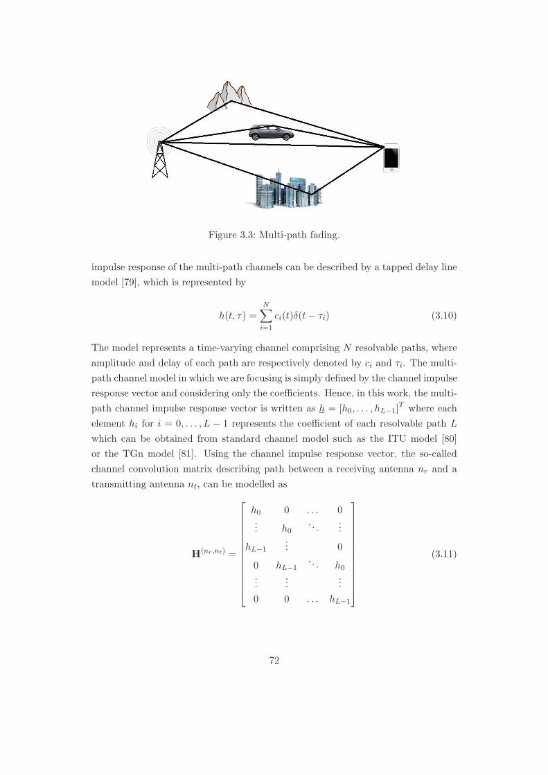
Figure 3.3: Multi-path fading.

impulse response of the multi-path channels can be described by a tapped delay line

model [79], which is represented by

h(t, τ) =N∑

i=1

ci(t)δ(t− τi) (3.10)

The model represents a time-varying channel comprising N resolvable paths, where

amplitude and delay of each path are respectively denoted by ci and τi. The multi-

path channel model in which we are focusing is simply defined by the channel impulse

response vector and considering only the coefficients. Hence, in this work, the multi-

path channel impulse response vector is written as h = [h0, . . . , hL−1]T where each

element hi for i = 0, . . . , L − 1 represents the coefficient of each resolvable path L

which can be obtained from standard channel model such as the ITU model [80]

or the TGn model [81]. Using the channel impulse response vector, the so-called

channel convolution matrix describing path between a receiving antenna nr and a

transmitting antenna nt, can be modelled as

H(nr,nt) =

h0 0 . . . 0... h0

. . ....

hL−1... 0

0 hL−1. . . h0

......

...

0 0 . . . hL−1

(3.11)

72

The channel convolution matrix is (N +L−1)×N dimensional matrix, where N is a

system processing gain and L is a number of the multi-path rays. The MIMO channel

can be formulated by pulling the channel matrices between antennas together, which

assume links between each antenna are uncorrelated links. The MIMO channel

model is formulated as

H =

H(1,1) . . . H(1,NT )

.... . .

...

H(NR,1) . . . H(NR,NT )

(3.12)

where the maximum number of receiving antennas and transmitting antennas are

given as NR and NT respectively.In the MIMO-HSDPA system, it is assumed that

the channel model is known at both transmitters and receivers, as the receivers

can send information regarding the channel state information to the transmitter via

feedback loops.

3.3.3 The MIMO-HSDPA Non-Successive Interference

Cancellation (SIC) Receiver Model

At the receiver, a signal received by each nr antenna is passed to a down-frequency

converter in order to shift the received signal back to the base band. After that, the

base-band received signal is delivered to a matched-filter for detection. The output

of the matched filter is sampled in every chip periods to produce the received signal

vectors rTnr(ρ). The received chip vector is obtained by concatenating the received

vectors from all received antennas, as the following

r(ρ) =[rT1 (ρ), . . . , rTnr

(ρ), . . . , rTNR(ρ)

]T(3.13)

The matched filter received signal vector corresponds to the transmitted vector z(ρ),

which is transmitted over the ρ symbol period. However, the dimension of the

receiver vector is NR(N +L− 1), which is longer than the length of the vector z(ρ),

since the signal is transmitted over a multi-path channel and is corrupted by the

ISI. The vector r(ρ) can be written as a function of the vector z(ρ), that is

r(ρ) = Hz(ρ) + H1z(ρ− 1) + H2z(ρ + 1) + n(ρ) (3.14)

where z(ρ−1) and z(ρ+1) are the signal vectors transmitted in the previous symbol

period and in the next symbol period respectively. The vector n(ρ) denotes the

73

noise power received at the output of the matched filter. The matrix H1 represents

a channel state in the previous symbol period whilst the matrix H2 is for the next

symbol period, these matrices are formulated as

H1 = (INR⊗ (JT )N )H

H2 = (INR⊗ JN )H

(3.15)

The previous and the next channel state matrices are constructed by using a shifting

matrix J. The matrix (JT )N move up the column of the target matrix by N positions

and place a group of zeroes in the empty space. Similarly, the matrix JN is used to

move columns of the target matrix down instead. Given a notation JN+L−1, the J

matrix is formulated as a (N +L− 1)× (N +L− 1) dimensional matrix, and it can

be written as

JN+L−1 =

0T(N+L−1)−1 0

I(N+L−1)−1 0(N+L−1)−1

(3.16)

The complete received signal is a NR(N + L− 1) ×N (x) dimensional matrix which

is constructed by gathering all vectors r(ρ) received during one Transmission Time

Interval (TTI) period together. The matrix is given as

R =[r(1), . . . , r(ρ), . . . , r(N (x))

](3.17)

Since the signal travels over a frequency selective channel, a multi-code received

signal vector might lose their orthogonality which creates ISI in the received symbols.

In order to mitigate the effect of the ISI, MMSE equalizer can be employed to

improve the detection. Once the ISI is alleviated, the de-spreading process then can

be run to recover the transmitted symbols afterward. In this work, it is assumed that

the restoration of code orthogonality and the de-spreading process are performed

simultaneously. The MMSE equalizer matrix is formulated as W = [w1, . . . , wK∗ ],

which is a NR(N +L− 1)×K∗ dimensional matrix. Each column of the W matrix

is a de-spreading coefficient vector for a channel k which is determined to minimize

a mean-square-error (MSE) and is obtained as

wk =C−1q

k

qHkC−1q

k

(3.18)

74

where C is the covariance matrix of the received signal vector and a vector qk

is

obtained from column kth a chip matched filter matrix. The matched filter matrix

is denoted by the matrix Q, which has the dimension of NR(N + L− 1) ×K∗, and

is determined as

Q = HS =[q1, . . . , q

K∗

](3.19)

The covariance matrix C is NR(N + L − 1) × NR(N + L − 1) dimensional matrix

and it can be calculated as follows

C = Qe(I3 ⊗A2)QHe + 2σ2INR(N+L−1) (3.20)

where σ2 is the variance of the system noise and the matrix Qe is a matched filter

matrix extended to the previous symbol period and the next symbol period for

including the ISI effect. The Qe matrix has the dimension of NR(N +L− 1)× 3K∗

and is given as Qe = [Q,Q1,Q2] where Q1 and Q2 are the matched filter matrix

for the previous symbol period and the next symbol periods respectively. Both Q1

and Q2 can be constructed by using the shifting matrix J such that

Q1 = (INR⊗ (JT

N+L−1)N )Q =

[q1,1

, . . . , qk,1

, . . . , qK∗,1

]

Q2 = (INR⊗ JT

N+L−1)Q =[q1,2

, . . . , qk,2

, . . . , qK∗,2

] (3.21)

Once the received signal vector is de-spread by the MMSE equalizes, the estimated

transmitted symbol is obtained as

y(ρ) = [y1(ρ), . . . , yK∗ ] = WHr(ρ) (3.22)

Then, the de-spread symbol matrix X can be generated from the vector y(ρ), which

is

X =[y(1), . . . , y(ρ), . . . , y(N (x))

]T= [x1, . . . , xK∗ ] (3.23)

where each column of the matrix X represents the estimated version of symbols

carried over each transmission channel. These symbols passed to a decision process

and de-coding process in order to recover the original binary data stream uk,D for

k = 1, . . . ,K∗. The non-SIC receiver structure is shown in Figure 3.4

75

Figure 3.4: The non-SIC receiver structure [53].

3.3.4 The MIMO-HSDPA Successive Interference Cancellation

Receiver Model

Since a multi-code communication employed in the transmission, it is feasible to use

an SIC receiver to improve signal-to-interference-noise ratio (SINR) at the receiver.

The idea of the SIC approach is, if some signal in a multi-code signal is received and

de-coded correctly at the receiver, that signal can be used to reduce the interference

in the multi-code signal, which facilitates receiving processes for the other channels.

For example, in HSDPA systems, signals in each channel are separated by code words

and are transmitted in parallel. At the receiver, a signal transmitted in the first code

is detected and is de-decoded, and if it is done correctly, the first signal is subtracted

from the received signal. Consequently, the process for recovering the second signal is

easier, as the interference from the first code is removed. The SIC process continuous

for the second signal and so on, which should successively improve the performance.

Note that, in order to maximize the performance of the SIC technique signal to be

removed should be in an descending order of the interference level, the first signal

causes stronger interference than the second signal and the second signal is stronger

than the third signal and so on. In this work, the SIC is performed channel by

channel starting from k = K∗ and the process is run till k = 1 for the last channel.

When de-spread for kth channel, a received signal matrix Rk is given, the subscript

k represents that the matrix Rk is used only for determining estimated symbols for

the kth channel. Since the SIC process begins from the K∗ channel, the received

signal matrix in (3.17) is written as RK∗ for an initialization. After the receiving

76

process for the kth channel is completed, the received signal matrix is modified to

be used for processing of the next channel as

Rk−1 = Rk −√EkΦk (3.24)

where the k index is run from k = K∗ to k = 1. The√Ek denotes the amount of

energy. the system allocated to the kth channel and the Φk is given as

Φk = qkxTk,D + q

k,1xTk,D1 + q

k,2xTk,D2 (3.25)

where the xk,D is a reproduction of a transmitted symbol vector of the kth channel,

which is generated by the receiver. Basically, when operating the SIC approach, the

received signal matrix is de-spread by the MMSE equalizer to obtain an estimated

symbol vector on each channel k, which is xTk = wHk Rk. The vector xk is then

de-modulated and de-coded to produce a binary stream vector given as uk,D. As-

suming that the vector uk,D is correctly detected same as the original vector uk, the

receiver then utilizes this vector to reproduce the transmitted symbol vector as the

xk,D, which exploits in (3.25) for an interference cancellation purpose. The vector

xk,D1and xk,D2 can be constructed by using the shifting matrix J, which is

xk,D1 = JN(x)xk,D

xk,D2 = JTN(x)xk,D

(3.26)

qk,q

k,1and q

k,2are matched filter chip vectors for the kth channel and are given in

(3.19) and (3.21) respectively. The SIC receiver structure is given as in the Figure 3.5

More detail on the MIMO-HSDPA SIC receiver can be found on [53].

3.4 Resource Allocation on MIMO-HSDPA Systems

3.4.1 Rate allocation using the system value optimization approach

The problem focused on this section is how to maximize downlink throughput for a

single user such that the upper-bound capacity can be achieved. In the past, the sum

bit rate maximization problem was formulated as a minimizing sum MSE problem

subject to having limited transmission energy per user. Giving the MSE as ǫk and

the total transmission energy as ET the problem is formulated as a Lagrangian dual

77

Figure 3.5: The SIC receiver structure [53].

objective function, which is written as

L(ǫk, Ek, λ) =K∗∑

k=1

ǫk + λ(K∗∑

k=1

Ek − ET ) (3.27)

where λ is known as a Lagrangian multiplier. Solving the above equation yields

the optimal amount of energy to be loaded into the channel k, which minimizes

the MSE under the power constraint. The optimal bit rate bpk for the channel k

is then determined afterward. Since the required bit rate bpk is formulated as a

function of ǫk and Ek, the solution cannot be obtained directly and needs exhaust-

ing computation to get the answer. Therefore, work [53] proposed the system value

optimization to facilitate the rate allocation problem. The system value consists of

the mean value approach and the minimum value approach. Both are employed to

determine the optimum number of signature sequences as well as discrete bit rate

for each transmission channel, which render the optimum total data rate achieved

by the system without pre-energy calculation.The mean system and the minimum

system value can be applied on both the Non-SIC and SIC receivers. For the mean

system value approach, that it is able produce the total rate which is close to the

theoretical upper-bound. When the mean and minimum system value approach col-

laborates with energy allocation, they contributes to two resource allocation schemes,

the equal-energy-equal-SNR (EEES) approach and the equal-energy-equal-rate ap-

proach, which will be discussed in the following section.

78

3.4.2 Energy Allocation Techniques for MIMO-HSDPA Systems

Giving transmission power budget as ET , the transmitter needs to allocate energy

to each channel for k = 1, . . . ,K such that the energy constraints∑K

k=1Ek ≤ ET

is satisfied. The transmission energy must be allocated sufficiently to the channels

so that expected SINRs and subsequent allocated data rates are realizable at the

receivers. The standard MIMO-HSDPA employs the equal energy allocation, which

can guarantee only the smallest bit rate in all channels. This method has a low

complexity, but it does not optimize the total data rate. Alternatively, the total

data rate can be maximized by the mean system value discrete bit loading approach.

However, this scheme requires uniform SINR measured at the output of the de-

spreading unit at the receiver. As a result, to use the mean system value scheme,

the transmitters need an equal SINR energy loading scheme which run an iterative

calculation method for the energy allocation in order to provide identical received

SINRs. For the minimum system value discrete bit loading, the equal energy loading

approach, which employ in the standard MIMO-HSDPA system, can be used. The

use of the minimum system value and the equal energy allocation is named as equal-

energy-equal-rate (EEER) approach in this work. For the mean system value loading

approach where the equal SINR loading scheme is applied on, it is called equal-

energy-equal-SINR loading approach, which EEES is used for an abbreviation. The

EEER and the EEES approach also can be found on [53].

The EEER Resource Allocation Approach

The EEER loading approach can be applied on the standard MIMO-HSDPA system

where a number of channels k = 1, . . . ,K is operated. The minimum system value

determine the used bit rate, bp,min, which is the smallest rate. The optimum number

of channels, K∗min, is also identified by the minimum system value, which gives the

total transmission rate as RT,min = K∗minbp,min. Then, the energy for each channel

k channel is obtained from the equal energy loading given as

Ek =ET

K∗min

(3.28)

where ET is total transmission energy per symbol period. The EEER is a simple

algorithm and can be with both the non-SIC and the SIC receivers without any

modifications. The simulation representing performance of the EEER approach is

examined in the next section.

79

The EEES Resource Allocation Approach

The mean system value is employed to determine the allocated bit rate, bp,mean, and

the optimum number of channels, K∗mean. For the energy allocation in the non-SIC

systems, using the equal SNR loading scheme, energy allocated to each channel for

k = 1, . . . ,K∗mean is written as

Ek,i =λ∗k

qHkC−1

i−1qk(3.29)

where qk

is obtained from (3.19). The λ∗k is the target system value corresponding to

the bit rate bpk , the bit rate allocated to the channel k. The matrix C is determined

from (3.20) and it can be seen that it is formulated as a function of Ek for k =

1, . . . ,K∗mean. Therefore, giving i as an iteration number, Ek,i is a function of Ek,i−1

for k = 1, . . . ,K∗mean, which is the amount of energy calculated in the previous

iteration. Note that, (3.29) begins with i = 1 where Ek,0 is initialized as Ek,0 =ET

K∗

meanfor all channels and the iterative process is repeated until Ek,i ≈ Ek,i−1 for

all k channels or i is equal to IMAX , which is the maximum number. For systems

using the SIC technique, energy calculation in each channel can be simplified so that

the computational complexity decreases. Unlike the non-SIC system, the allocated

energy Ek,i for the SIC system is a function of itself in the previous iteration,Ek,i−1.

Moreover, in each Ek calculation, the stored covariance matrix C−1k−1, which is a

function of Ek−1,IMAX, is used instead of C−1

i−1. Consequently, a number of matrix

inversions need to be done for each Ek calculation is reduced significantly.To be more

specific, the total number of matrix inversion required to complete the algorithm is

equal to one. The allocated energy Ek for the SIC system is obtained as

Ek,i =γ∗k

ξ − ζ1,(i−1) |ξ3|2 − ζ2,(i−1)

(|ξ4|2 − 2ζ1,(i−1)ξ6 + ζ21,(i−1) |ξ5|

2 |ξ3|2) (3.30)

where γ∗k is a target SNR for a given bit rate bpk . For a given system gap, Γ, The

SNR target is given as

γ∗k(bpk) = Γ(2bpk − 1) (3.31)

The parameters in the denominator of (3.30) are the matrix inversion lemma’s pa-

rameter. The detail of the matrix inversion lemma and the calculation method of

the parameters can be found in [53] as well. Actually, (3.30) is performed in exact

order starting from evaluating the allocated energy for the first signature sequence.

80

The system firstly initializes C−10 by setting C−1

0 = 12σ2 INR(N+L−1) and (3.30) is

than operated iteratively till i = IMAX , where the E1 is achieved. Typically, the

IMAX is not a great number and (3.30) is converged after running for several times.

Once E1 is obtained, it is used to formulate the C−11 for calculating energy for the

next signature sequence. Using the matrix inversion lemma, there is no need to

invert any matrices in the formulation of the C−11 . The SIC equal SNR continues

till all Ek are calculated for k = 1, . . . ,K∗mean, As it can be seen, only one matrix

inversion is done, which is formulating C−10 , so that the computational cost for the

SIC EEES loading scheme is much lower than the non-SIC EEES scheme. The

simulation results for EEES will be given and discussed in the next section.

3.4.3 Simulations and Performance Comparison

The simulation results produced in this section replicates the original results pro-

duced in [53] by using LabVIEW [82], as the LabVIEW is main software to interface

with the test bed system which will be described next. The objective of replicat-

ing the results is to confirm that the computational performance of LabVIEW is

identical to MATLAB [83], which use to produce the result for [53]. The tests are

done on the ITU-R standard channel model given in [80], which is issued by The

International telecommunication union (ITU). The channel model used in this work

represents pedestrian test environments for Outdoor systems to Indoor systems. The

model comprises the multi-path fading channel A and channel B, where the channel

B has a longer delay time spread. Both channels are mostly encountered by users

in practice. To adapt the ITU model on the MIMO-HSDPA simulation system, the

ITU model is interpreted and is re-constructed by the method given in [53] such

that each channel impulse response in the new model is sampled at the chip period

of the MIMO-HSDPA system. The re-constructed channel is used as a prototype to

generate random channels having similar properties which will be used in the simu-

lations. The simulation results are presented as average total data rates achieved by

the receiver when applying each resource allocation approach on those multi-path

fading channels.

The Simulation Results and Discussion

The simulations for a 2 x 2 MIMO-HSDPA system are run on the LabVIEW platform

to evaluate the capacity, represented in bits per symbol, for each loading scheme.

The capacity curves are plotted against total received SNR per receiver, which is

81

Figure 3.6: The mean upper bound capacity curve for the pedestrian A channel.

given in dB.

Firstly, the upper bound capacity was determined using the water filling and the

system value optimization approach, demonstrated in [53].The upper bound curves

for the pedestrian A and the pedestrian B channels are shown in figure 3.6 and

figure 3.7 respectively. Note that, each curve given in the figures is a mean capacity

curve, which is determined from 10 different channels for both the pedestrian A

channel and pedestrian B channel. The curve corresponding to the water filling

approach with the non-SIC and the SIC techniques are shown under heading ”WF

UB” and ”SIC WF UB” whilst the system value approach are marked as ”SV UB”

and ”SIC SV UB”, for the non-SIC and SIC system respectively. It can be seen that

the system value and the iterative water filling approaches produce identical capacity

curves in both systems with the SIC and without the SIC receiver structures. Also,

the figures for the pedestrian A and the pedestrian B channels confirm that the

performance of the system value approach is comparable to the iterative water filling

approach.However, when considers the complexity, it can be said that the system

value approach gives the better performance, as the algorithm to perform the system

value calculation is shorter and less complicated compared with the iterative water

filling algorithm. Moreover, the simulation results also show that the SIC receiver

structure significantly improves the capacity. Especially in the high SINR region

where energy per channel is higher, the interference among the parallel channels

increases and eventually saturates the system throughput. However, when the SIC

82

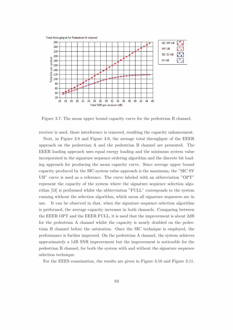
Figure 3.7: The mean upper bound capacity curve for the pedestrian B channel.

receiver is used, those interference is removed, resulting the capacity enhancement.

Next, in Figure 3.8 and Figure 3.9, the average total throughput of the EEER

approach on the pedestrian A and the pedestrian B channel are presented. The

EEER loading approach uses equal energy loading and the minimum system value

incorporated in the signature sequence ordering algorithm and the discrete bit load-

ing approach for producing the mean capacity curve. Since average upper bound

capacity produced by the SIC-system value approach is the maximum, the ”SIC SV

UB” curve is used as a reference. The curve labeled with an abbreviation ”OPT”

represent the capacity of the system where the signature sequence selection algo-

rithm [53] is performed whilst the abbreviation ”FULL” corresponds to the system

running without the selection algorithm, which mean all signature sequences are in

use. It can be observed in that, when the signature sequence selection algorithm

is performed, the average capacity increases in both channels. Comparing between

the EEER OPT and the EEER FULL, it is used that the improvement is about 2dB

for the pedestrian A channel whilst the capacity is nearly doubled on the pedes-

trian B channel before the saturation. Once the SIC technique is employed, the

performance is further improved. On the pedestrian A channel, the system achieves

approximately a 1dB SNR improvement but the improvement is noticeable for the

pedestrian B channel, for both the system with and without the signature sequence

selection technique.

For the EEES examination, the results are given in Figure 3.10 and Figure 3.11.

83

Figure 3.8: The mean capacity curve of the EEER approach on the pedestrian Achannel.

The EEES employs the mean system value method for selecting the optimum se-

quences and allocating the bit rate. The EEES approach needs to be operated using

iterative transmission energy adjustment scheme in order to produce identical re-

ceived SNRs in all channels at the de-spreading filter output. The iterative energy

calculation algorithm for the non-SIC and SIC systems are presented by (3.29) and

(3.30) respectively. For the energy calculation in the non-SIC system, in each iter-

ation, energy vector denoting the amount of energy allocated into each channel is

calculated and is compared to the energy vector obtained in the previous iteration.

The comparison gives a differential amount of energy for each channel which is used

as a condition to exit the iteration. In this work, the iterative energy calculation is

stop when the sum of differential energy is lower than 1% of the total transmission

energy or the number of the iterations reaches the maximum number IMAX For the

SIC receiver system, the iterative energy calculation is carried for each individual

channel k and the iteration will stop when the differential amount of energy in that

channel is lower than 1% of the initial energy of the channel, which is equal to ET /K.

As it can be seen, the EEES approach gives the higher capacity compared with

the EEER approach and, with the SIC receiver, the EEES approach achieves a near

upper bound capacity for the pedestrian A channel before the system is saturated.

The Interesting results that can be observed in the EEES approach is that once

the SIC is utilised, there is no need to do the signature sequence selection, as the

84

Figure 3.9: The mean capacity curve of the EEER approach on the pedestrian Bchannel.

performance of the SIC EEES OPT and SIC EEES FULL are similar in both testing

channels. This is because the SIC technique runs effectively when used in collabo-

ration with the EEES, which almost eliminates the interference. However, having

the signature sequence selection provide much better performance in the non-SIC

system, as it can be observed when compared the EEES OPT algorithm with the

EEES FULL algorithm in the pedestrian B channel.

The performance comparison between the EEES and EEER strategies are given

in Figure 3.12 and Figure 3.13. For both pedestrian A and pedestrian B channels,

it is observed that the use of the mean system value results in a higher through-

put than the use of minimum system value and, once the mean system value rate

allocation is incorporated with the signature sequence selection algorithm and the

SIC technique, an impressive performance can be achieved. As it can be seen in

the figures, represented by the SIC EEES OPT curve, the capacity produced by

making use of those techniques together is close to the upper bound curve for both

pedestrian channels A & B. To compare the mean system value with the minimum

system value approach, the capacities of the SIC EEES OPT and capacities of the

SIC EEER OPT are re-examined, and it is observed that the mean system value

produces a better throughput in all channels. For example, the capacity of the SIC

EEES OPT approach measured at 30 dB of SINR in the pedestrian A channel is 13%

higher than the capacity of the SIC EEER OPT approach. The results are more

85

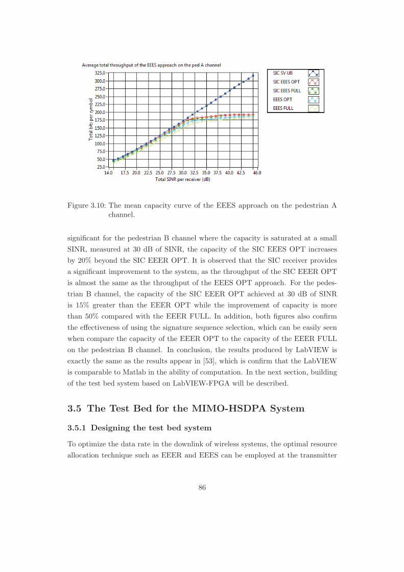
Figure 3.10: The mean capacity curve of the EEES approach on the pedestrian Achannel.

significant for the pedestrian B channel where the capacity is saturated at a small

SINR, measured at 30 dB of SINR, the capacity of the SIC EEES OPT increases

by 20% beyond the SIC EEER OPT. It is observed that the SIC receiver provides

a significant improvement to the system, as the throughput of the SIC EEER OPT

is almost the same as the throughput of the EEES OPT approach. For the pedes-

trian B channel, the capacity of the SIC EEER OPT achieved at 30 dB of SINR

is 15% greater than the EEER OPT while the improvement of capacity is more

than 50% compared with the EEER FULL. In addition, both figures also confirm

the effectiveness of using the signature sequence selection, which can be easily seen

when compare the capacity of the EEER OPT to the capacity of the EEER FULL

on the pedestrian B channel. In conclusion, the results produced by LabVIEW is

exactly the same as the results appear in [53], which is confirm that the LabVIEW

is comparable to Matlab in the ability of computation. In the next section, building

of the test bed system based on LabVIEW-FPGA will be described.

3.5 The Test Bed for the MIMO-HSDPA System

3.5.1 Designing the test bed system

To optimize the data rate in the downlink of wireless systems, the optimal resource

allocation technique such as EEER and EEES can be employed at the transmitter

86

Figure 3.11: The mean capacity curve of the EEES approach on the pedestrian Bchannel.

whilst the receiver can use the SIC technique, as described by [53]. These tech-

niques are simulated on LabVIEW by using a MIMO-HSDPA link level model, as

demonstrated in the previous section, and they have been shown the capability of

enhancing the downlink throughput of the systems. These techniques are promising

to be used in the wireless systems such as IEEE 802.11 the wireless LAN to provide

the better experience to users. When designing the test bed for the communication

systems, there are two majors problem to be concerned. The first problem is the

amount of data to be transferred between radio front ends and processing units.

The second problem is synchronization between the transmitter and the receiver.

The data transfer load between the baseband device and the processing unit is

concerned because sometime it is massive and exceed the current bandwidth of the

medium. For example, if the testbed system is set up for the HSDPA transmission

which uses a WCDMA technique for channel access. According to UMTs standard,

this system need to be run on a 2 GHz carrier frequency band with a 5 MHz carrier

bandwidth in a downlink channel. Now for the testbed system, it is assumed that

the system employs a 16 bits Digital to Analogue Convertor (DAC) and an Analogue

to Digital Convertor (ADC). The Ethernet is used to link between the host machine

and the radio devices, as the following Figure 3.14

For 5 MHz bandwidth, according to the Nyquist sampling theorem, the minimum

sampling rate that can be used in the system is 10 MHz. Therefore, the transmitter

87

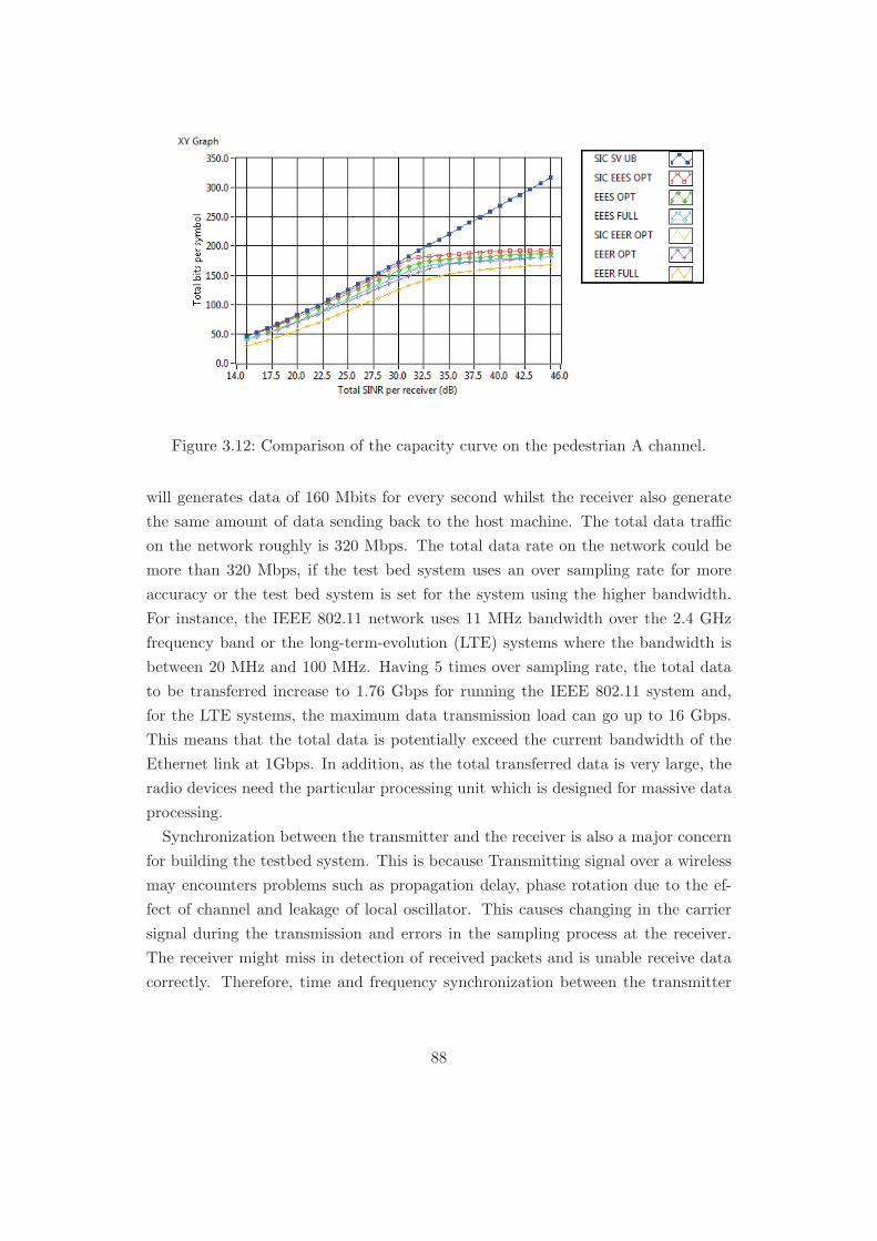
Figure 3.12: Comparison of the capacity curve on the pedestrian A channel.

will generates data of 160 Mbits for every second whilst the receiver also generate

the same amount of data sending back to the host machine. The total data traffic

on the network roughly is 320 Mbps. The total data rate on the network could be

more than 320 Mbps, if the test bed system uses an over sampling rate for more

accuracy or the test bed system is set for the system using the higher bandwidth.

For instance, the IEEE 802.11 network uses 11 MHz bandwidth over the 2.4 GHz

frequency band or the long-term-evolution (LTE) systems where the bandwidth is

between 20 MHz and 100 MHz. Having 5 times over sampling rate, the total data

to be transferred increase to 1.76 Gbps for running the IEEE 802.11 system and,

for the LTE systems, the maximum data transmission load can go up to 16 Gbps.

This means that the total data is potentially exceed the current bandwidth of the

Ethernet link at 1Gbps. In addition, as the total transferred data is very large, the

radio devices need the particular processing unit which is designed for massive data

processing.

Synchronization between the transmitter and the receiver is also a major concern

for building the testbed system. This is because Transmitting signal over a wireless

may encounters problems such as propagation delay, phase rotation due to the ef-

fect of channel and leakage of local oscillator. This causes changing in the carrier

signal during the transmission and errors in the sampling process at the receiver.

The receiver might miss in detection of received packets and is unable receive data

correctly. Therefore, time and frequency synchronization between the transmitter

88

Figure 3.13: Comparison of the capacity curve on the pedestrian B channel.

Radio 1, Tx machine

I/Q

modulation 16 bits ADC

I/Q

modulation 16 bits DAC

Radio 2, Rx machine

Host computer (simulating

5MHz bandwidth system

and using 16 bits ADC)

Lo

ca

l are

a n

etw

ork

(Eth

ern

et)

320Mbits/sec

160Mbits/sec

160Mbits/sec

Figure 3.14: The SDR system.

and the receiver is required in the signal reception. The synchronization is possibly

done by using external clock signal source connecting between the transmitter and

the receiver, but it requires a precise signal source, which is very expensive.

In this section, a time, frequency and phase synchronization method for the test

bed system is presented. Using this method, the synchronization is operated only

based on a signal processing method without any requirement of external signal

sources. The synchronization is employed in the test bed system which is built from

the LabVIEW-PXIe system, provided by National Instrument (NI). The reason of

using LabVIEW and the PXIe system because PXIe is very flexible that come with

many modules designed for particular works such as the NI 5791 the vector signal

transceiver module, which is capable of doing MIMO beamforming configurations.

89

In addition, LabVIEW simplifies building the testbed system because using only

LabVIEW can create both windows based-software and FPGA applications, which

generally requires the expertise in several programming language. The LabVIEW-

PXIe system is therefore a solution for making a testbed for ultra wideband trans-

mission systems. Moreover, the LabVIEW-FPGA testbed system is compatible with

a channel emulator software provided by National Instrument. The channel emu-

lator is employed to generate realistic multi-path environments for the the testbed

system. The LabVIEW-PXIe system is used to examined the EEER and EEES with

SIC or non-SIC receivers.

3.5.2 Time and frequency Synchronization in the Test Bed System

When transmitting signals over a wireless channel, received signals basically not only

experiencing propagation delay but also encounters attenuation and random phase

due to the channel. This causes reduction in amplitude and phase rotation in the

received signal, as a result, the receiver might be fail in detection. When performing

signal transmission on real devices, more practical problems are introduced. As

conducted by [84], this works transmit a complex sinusoidal signal over a wireless

channel by using the USRP devices. Since the transmission distance is not far, the

channel can be considered as a slow flat fading channel. It has been found that, apart

from the effects of channel, there are two more problems due to the transmission

devices.

The first problem is shifting in carrier frequency, which adds more phase rotation

in the received signal. For transmitting a signal, the transmitter basically convert

the signal presented in a baseband frequency to a passband frequency before the

transmission. This process done by the USRP device by using a local oscillator,

which generates the passband signal at the frequency of Fc,Tx, which is a carrier

frequency. At the receiver, a reverse process is performed by shifting the frequency of

the received signal back from the passband frequency to the baseband frequency. The

down-conversion process is operated by using a frequency Fc,Rx generated by another

local oscillator. Since there is no common clock signal to be used as a reference, the

transmitter and the receiver is not synchronized so that there is discrepancy in the

frequency, written as ∆Fc = Fc,Tx − Fc,Rx. This frequency offset produces another

phase rotation in the received signal.

The second problem is called local oscillator leakage (LO). The LO problem is

caused by impairment of the hardware and it yields extra spectral components

90

around the baseband DC level component. When producing the signal constel-

lation at the receiver, the LO appears as extra noise dots around the zero point in a

received constellation diagram. The LO problem arises in both the transmitter end

and the receiver end and also need to be removed.

Therefore, without an external signal source for synchronization, there are several

problems need to be solved for transmission and reception of signals in the test bed

system. The first problem is how the time synchronization between the transmit-

ter and the receiver is performed such that the receiver can detect the transmitted

signal. The second problem is, once the signal is detected, how to eliminate the

phase rotation and the extra noise in order to receive the constellation diagram cor-

rectly, this problem is called frequency synchronization problem. In this work, the

problems can be solved by using signal processing methods at the transmitter and

at the receiver. At the transmitter, data to be transmitted is formed as packets

where each packet is added by redundant signals for synchronization purpose. At

the receiver, post-signal processing is operated by using the extra signals inserted by

the transmitter. Hence, the receiver can perform both time and frequency synchro-

nization accordingly. This method has been employed by [84] for transmit a signal

using USRP devices and MATLAB and it will be applied to be used for building

the LabVIEW-PXI test bed system.

The Time Synchronization by Using a Chirp Signal

For the data transmission, a binary data sequence is firstly en-coded and is mapped

into symbols by a QAM modulator. Since multi-code channels are employed in the

MIMO-HSDPA transmission, the symbols are organized as a transmission matrix

as represented by (3.1).After that, those symbols are spread by signature sequences

to create a multi-code channel transmission and transmission energy is allocated

into each channel afterward. The transmission signal is formulated as a vector

znt(ρ) = SntAy (ρ) for each symbol period and the transmission vectors znt

are

organized as (3.3) to represent vector signals to be transmitted in the entire symbol

period. In order to transmit the signal as in (3.3) using the time synchronization

and frequency synchronization, the matrix in (3.3) is firstly re-organized as a vector,

where the length of the new vector is equal to N ×Nt×N (x).The vector then passed

to a pulse shaping filter to formulate transmission pulses. The square root raise

cosine pulse shaping filter is used to achieve more spectral efficiency. Using the

pulse shaping filter limits bandwidth of each symbol and ensure that the ISI does

91

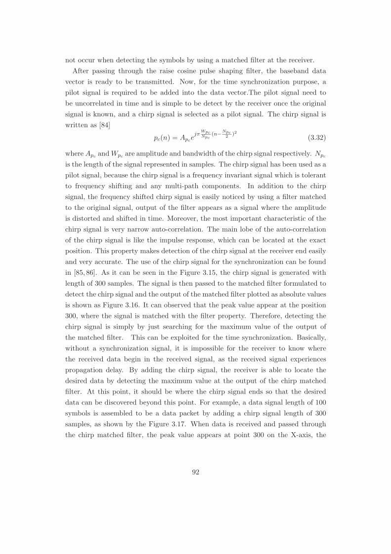
not occur when detecting the symbols by using a matched filter at the receiver.

After passing through the raise cosine pulse shaping filter, the baseband data

vector is ready to be transmitted. Now, for the time synchronization purpose, a

pilot signal is required to be added into the data vector.The pilot signal need to

be uncorrelated in time and is simple to be detect by the receiver once the original

signal is known, and a chirp signal is selected as a pilot signal. The chirp signal is

written as [84]

pc(n) = Apcejπ

WpcNpc

(n−Npc2

)2(3.32)

where Apc and Wpc are amplitude and bandwidth of the chirp signal respectively. Npc

is the length of the signal represented in samples. The chirp signal has been used as a

pilot signal, because the chirp signal is a frequency invariant signal which is tolerant

to frequency shifting and any multi-path components. In addition to the chirp

signal, the frequency shifted chirp signal is easily noticed by using a filter matched

to the original signal, output of the filter appears as a signal where the amplitude

is distorted and shifted in time. Moreover, the most important characteristic of the

chirp signal is very narrow auto-correlation. The main lobe of the auto-correlation

of the chirp signal is like the impulse response, which can be located at the exact

position. This property makes detection of the chirp signal at the receiver end easily

and very accurate. The use of the chirp signal for the synchronization can be found

in [85, 86]. As it can be seen in the Figure 3.15, the chirp signal is generated with

length of 300 samples. The signal is then passed to the matched filter formulated to

detect the chirp signal and the output of the matched filter plotted as absolute values

is shown as Figure 3.16. It can observed that the peak value appear at the position

300, where the signal is matched with the filter property. Therefore, detecting the

chirp signal is simply by just searching for the maximum value of the output of

the matched filter. This can be exploited for the time synchronization. Basically,

without a synchronization signal, it is impossible for the receiver to know where

the received data begin in the received signal, as the received signal experiences

propagation delay. By adding the chirp signal, the receiver is able to locate the

desired data by detecting the maximum value at the output of the chirp matched

filter. At this point, it should be where the chirp signal ends so that the desired

data can be discovered beyond this point. For example, a data signal length of 100

symbols is assembled to be a data packet by adding a chirp signal length of 300

samples, as shown by the Figure 3.17. When data is received and passed through

the chirp matched filter, the peak value appears at point 300 on the X-axis, the

92

Figure 3.15: A chirp signal.

QAM data then can be found at point 301 to point 401.

Eliminating the Local Oscillator (LO) Leakage and Frequency

Synchronization Using a Sinusoidal Pilot Signal

Before performing the frequency synchronization, the LO leakage should be firstly

removed. As the LO leakage component appears around the baseband, centered at

the zero frequency in the frequency domain. Basically, the LO leakage is simply

eliminate by the use of a filter. However, filtering the LO leakage out directly will

remove some desired signal component, because the LO leakage is mixed with the

signal baseband. Therefore, in order to avoid filtering out the necessary components

when removing the LO leakage, the baseband signal must be shift in frequency away

from the LO leakage.

The shifting in frequency of the baseband signal can be done by multiplying the

signal by the sinusoidal signal. However,due to shifting in frequency, this will limit

the bandwidth of the original signal so that the signal bandwidth must be concerned

when operating the frequency shift.After passing through the filter, the received

signal will converted back to the original frequency. The LO leakage is caused by

transmission devices and it exists only in the USRP devices. In the LabVIEW-PXIe

93

Figure 3.16: The auto-correlation of the chirp signal.

system, the hardware is improved so that the LO leakage problem does not exist,

shifting in frequency of the baseband signal is not necessary.

A discrepancy in carrier frequency of the transmitter and the receiver is deter-

mined as the frequency offset, which is ∆Fc,rx = Fc,tx − Fc,rx. Note that, the

frequency offset also includes a phase rotation due to the communication channel.

In order to synchronize the frequency between the transmitter and the receiver, a

contemporary method using a pilot signal for channel observation is employed in this

work.Although the pilot signal approach require to transmit redundant information

which is waste of bandwidth and reduce the effective data rate, it is more accurate

and is simpler than others such as a blind detection scheme [87]. Moreover, the

sinusoidal pilot signal approach suits current resources and facilities available to us

at that time.The training sinusoidal signal is inserted in between the chirp signal

and the data signal and it acts as a pilot signal which observes all channel effects.

At the receiver, the pilot sinusoidal signal will be compared with the original signal,

94

Figure 3.17: A chirp signal added at the beginning of a message signal.

generated by the receiver, so that the receiver is able to know how the carrier fre-

quency is affected the channel and can recover the original frequency of the message.

The sinusoidal pilot signal is given as [84]

Ps(n) = APsej2πfPsn, 0 ≤ n < NPs (3.33)

where APc and FPs is amplitude and frequency of the signal given in cycles/samples

respectively. It is advised that the pilot signal should not be too long, as it will

increase the overhead of the data packet. In the work, the sinusoidal pilot signal

is length of 1000 samples. The packet to be transmitted comprises with two pilot

signals, the chirp signal and the sinusoidal signal, is given as in the Figure 3.18.

At the receiver, the chirp signal is firstly processed to determine the beginning of

the received data. Once the received data is known, the sinusoidal signal will be

extracted for implementing the frequency synchronization. The received sinusoidal

95

Figure 3.18: Transmission data added by two pilot signals.

signal can be written as

Ps,Rx(n) =(αAPse

j(2πfPsn−φh) + w(n))ej2π∆fcn

= αAPsej(2π(fPs+∆fc)n−φh)) + wc(n)

(3.34)

Where wc(n) = w(n)ej2π∆fcn. For knowing the frequency and the amplitude, the

sinusoidal pilot signal can be reconstructed as Ps(n) by the receiver and it will be

compared with the Ps,Rx to achieve the normalized frequency offset signal as

sfc(n) =Ps,Rx(n)Ps(n)∗

|E [Ps,Rx(n)Ps(n)∗|]

= ej(2π∆fcn−φh) + wcp(n)

(3.35)

It can be seen that, the frequency synchronization is still be a noisy signal so that a

filter is required to eliminate the noise. The signal sfc is then passed to the Low-Pass

Filter (LPF). After that, the auto-correlation at 1 sample delay of the output of the

low-pass filter is operated in order to obtain only the signal, which is as

E [sfc,LPF (n)sfc,LPF (n + 1)∗] = e−j2π∆fc (3.36)

Having (3.36) the frequency offset ∆fc can be calculated by using

∆fc = E [sfc,LPF1(n)sfc,LPF2(n)∗] (3.37)

The vector signal sfc,LPF1 begins from the first element to the length of Nps − 1,

where Nps is the maximum number of the sample of the signal and sfc,LPF2 begins

96

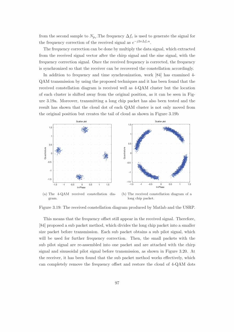
from the second sample to Nps .The frequency ∆fc is used to generate the signal for

the frequency correction of the received signal as e−j2π∆fcn.

The frequency correction can be done by multiply the data signal, which extracted

from the received signal vector after the chirp signal and the sine signal, with the

frequency correction signal. Once the received frequency is corrected, the frequency

is synchronized so that the receiver can be recovered the constellation accordingly.

In addition to frequency and time synchronization, work [84] has examined 4-

QAM transmission by using the proposed techniques and it has been found that the

received constellation diagram is received well as 4-QAM cluster but the location

of each cluster is shifted away from the original position, as it can be seen in Fig-

ure 3.19a. Moreover, transmitting a long chip packet has also been tested and the

result has shown that the cloud dot of each QAM cluster is not only moved from

the original position but creates the tail of cloud as shown in Figure 3.19b

-1.5 -1 -0.5 0 0.5 1 1.5

-1.5

-1

-0.5

0

0.5

1

1.5

Qu

ad

ratu

re

In-Phase

Scatter plot

(a) The 4-QAM received constellation dia-gram.

-1.5 -1 -0.5 0 0.5 1 1.5-1.5

-1

-0.5

0

0.5

1

1.5Q

ua

dra

ture

In-Phase

Scatter plot

(b) The received constellation diagram of along chip packet.

Figure 3.19: The received constellation diagram produced by Matlab and the USRP.

This means that the frequency offset still appear in the received signal. Therefore,

[84] proposed a sub packet method, which divides the long chip packet into a smaller

size packet before transmission. Each sub packet obtains a sub pilot signal, which

will be used for further frequency correction. Then, the small packets with the

sub pilot signal are re-assembled into one packet and are attached with the chirp

signal and sinusoidal pilot signal before transmission, as shown in Figure 3.20. At

the receiver, it has been found that the sub packet method works effectively, which

can completely remove the frequency offset and restore the cloud of 4-QAM dots

97

to the original position. The sub packet approach is included with the time and

frequency synchronization in order to construct the LabVIEW-PXI test bed system.

The detail of how the LabVIEW-PXIe testbed system is constructed can be found

Figure 3.20: A transmission data using 4 sub packets.

in the appendix I.

3.6 Performance Evaluation on the MIMO-HSDPA

Test Bed System

This section demonstrates the performance of the proposed resources allocation tech-

niques when running on the test bed set up for a MIMO-HSDPA system. The test

bed performs real-time FPGA transmission collaborating with the channel emu-

lator software to generate the test environment, which is suitable to evaluate the

performance of the approaches.

The MIMO-HSDPA to be operated is modeled as shown in the section 2. The

system comprises a 2 x 2 MIMO transmission running on the standard HSDPA sys-

tem. The transmitter generates 4-QAM symbols and transmits over coded-channels

according to WCDMA multi-coded communication. The OVSF code is used in the

spreading process. The processing gain of the OVSF code is set to 16 and 16 parallel

98

signature sequence can be used in the SISO mode. The OVSF code is extended to

32 parallel sequences for the MIMO transmission by using the method described in

the section 1.3.1. The transmitter runs the EEES and EEER approach, as described

in [58], to allocate energy and data rate to each coded- channel and the transmission

signal vector is then formulated. The signal vector is covert to RF frequency band

by the up converter, in this work the 2.45 GHz is employed for the RF frequency.

The transmission bandwidth is set to be 5 MHz and the chip rate of 3.84 MHz is

used to transmit the WCDMA signal. Both data transmission with and without the

signature sequence ordering and the channel selection technique were examined.

At the receiver, the received signal is down-converted and is sampled. After

sampling, the sampled signal is convolved with a vector of channel impulse samples

corresponding to a channel impulse response set generated input power delay profile.

Note that, the pedestrian A channel power delay profile specifiedby the ITU is uti-

lized in this work. The down conversion and the convolution of signal are performed

by the FPGA emulator. The emulator then passes the result to the host machine to

operated de-spreading afterward. The MMSE equalizer is utilized for de-spreading.

The SIC or non-SIC receiver will collaborate with the MMSE equalizer in order to

recover the original symbols. Both non-SIC and SIC were also evaluated. After de-

spreding process, the receiver sent the channel impulse response vector back to the

transmitter as channel state information. The transmitter will use this information

in order to calculate and allocate resource for the next transmission.

3.6.1 On the Performance of The Test Bed System

This section compared the results produced by the LabVIEW-PXIe test bed system

with the results obtained from the simulations. The objective is to show that the test

bed is realistic and can be used to collect the results for the MIMO-HSDPA system.

The set of results provided in this section were collected over 50 random pedestrian

A channels and will be presented as mean received SNR for each communication

channel.

The first set of the results comprises 4 main figures, where each figure consists of 4

sub-figures representing the mean SNR of the coded-channel simulated on different

transmission energy value. Each main figure corresponds to the proposed technique,

EEES or EEER, collaborating with or without the channel selection approach. When

using the channel selection technique [53] yields the optimum number of parallel

coded channel so that the figure labeled by OPT whilst the figure labeled by FULL

99

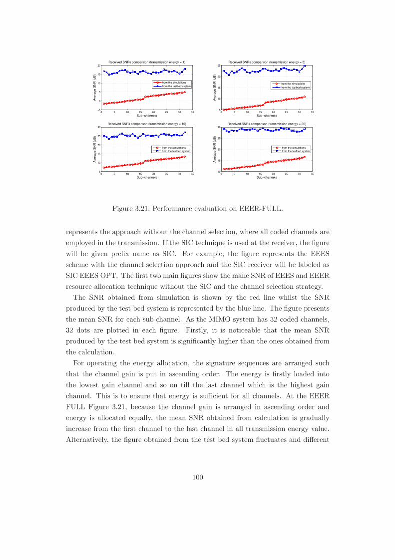
0 5 10 15 20 25 30 35−5

0

5

10

15

20

Sub−channels

Avera

ge S

NR

(dB

)

Received SNRs comparison (transmission energy = 1)

from the simulations

from the testbed system

0 5 10 15 20 25 30 355

10

15

20

25

Sub−channels

Avera

ge S

NR

(dB

)

Received SNRs comparison (transmission energy = 5)

from the simulations

from the testbed system

0 5 10 15 20 25 30 355

10

15

20

25

30

Sub−channels

Avera

ge S

NR

(dB

)

Received SNRs comparison (transmission energy = 10)

from the simulations

from the testbed system

0 5 10 15 20 25 30 3510

15

20

25

30

Sub−channels

Avera

ge S

NR

(dB

)

Received SNRs comparison (transmission energy = 20)

from the simulations

from the testbed system

Figure 3.21: Performance evaluation on EEER-FULL.

represents the approach without the channel selection, where all coded channels are

employed in the transmission. If the SIC technique is used at the receiver, the figure

will be given prefix name as SIC. For example, the figure represents the EEES

scheme with the channel selection approach and the SIC receiver will be labeled as

SIC EEES OPT. The first two main figures show the mane SNR of EEES and EEER

resource allocation technique without the SIC and the channel selection strategy.

The SNR obtained from simulation is shown by the red line whilst the SNR

produced by the test bed system is represented by the blue line. The figure presents

the mean SNR for each sub-channel. As the MIMO system has 32 coded-channels,

32 dots are plotted in each figure. Firstly, it is noticeable that the mean SNR

produced by the test bed system is significantly higher than the ones obtained from

the calculation.

For operating the energy allocation, the signature sequences are arranged such

that the channel gain is put in ascending order. The energy is firstly loaded into

the lowest gain channel and so on till the last channel which is the highest gain

channel. This is to ensure that energy is sufficient for all channels. At the EEER

FULL Figure 3.21, because the channel gain is arranged in ascending order and

energy is allocated equally, the mean SNR obtained from calculation is gradually

increase from the first channel to the last channel in all transmission energy value.

Alternatively, the figure obtained from the test bed system fluctuates and different

100

0 5 10 15 20 25 30 350

5

10

15

20

Sub−channels

Avera

ge S

NR

(dB

)

Received SNRs comparison (transmission energy = 1)

from the simulations

from the testbed system

0 5 10 15 20 25 30 355

10

15

20

25

Sub−channels

Avera

ge S

NR

(dB

)

Received SNRs comparison (transmission energy = 5)

from the simulations

from the testbed system

0 5 10 15 20 25 30 355

10

15

20

25

30

Sub−channels

Avera

ge S

NR

(dB

)

Received SNRs comparison (transmission energy = 10)

from the simulations

from the testbed system

0 5 10 15 20 25 30 3510

15

20

25

30

Sub−channels

Avera

ge S

NR

(dB

)

Received SNRs comparison (transmission energy = 20)

from the simulations

from the testbed system

Figure 3.22: Performance evaluation on EEES-FULL.

from the figure obtained from the calculation. This is because the channel seen by

the receiver is corrupted by random phase change which makes the channel to be

different from the channel known by the transmitter. The receiver utilizes the same

set of signature sequence as used by the transmitter in de-spreading process but the

channel is random so that the figure varies around the average value. Note that,

there is no slope on the figure of the test bed system as the transmission energy

allocated equally.

At the EEES FULL Figure 3.22, it can be seen that the mean SNR achieved

from calculation is almost identical in all channels as the transmitter calculates and

allocates energy sufficiently for each channel to get the uniform SNR. For the figure

produced by the test bed system, as the channel gain is put in ascending order,

the energy therefore allocates in descending order to compensate the channel gain.

However, it is observed from the test bed system that the mean SNR is not equal

and gently decrease from the first channel to the last channel. When channel gain

fluctuates at the receiver, it seems that the mean received SNRs are influenced only

by the allocated energy. Therefore, the mean SNR has a descending slope, which is

matched to energy allocation performed by the EEES approach.

Figures 3.24 and Figure 3.25 show the result of the EEER and EEES when the

channel selection technique is incorporated. Once the channel selection approach is

employed, some of channel is removed as it is a low gain channel. Consequently,

101

0 5 10 15 20 25 30 350

5

10

15

20

25

Sub−channels

Avera

ge S

NR

(dB

)

Received SNRs comparison (transmission energy = 1)

from the simulations

from the testbed system

0 5 10 15 20 25 30 3510

15

20

25

30

Sub−channels

Avera

ge S

NR

(dB

)

Received SNRs comparison (transmission energy = 5)

from the simulations

from the testbed system

0 5 10 15 20 25 30 3510

15

20

25

30

35

Sub−channels

Avera

ge S

NR

(dB

)

Received SNRs comparison (transmission energy = 10)

from the simulations

from the testbed system

0 5 10 15 20 25 30 3515

20

25

30

35

Sub−channels

Avera

ge S

NR

(dB

)

Received SNRs comparison (transmission energy = 20)

from the simulations

from the testbed system

Figure 3.23: Performance evaluation on EEER-OPT.

the system achieves the higher SNR in all transmission energy value, which can be

observed from both the figure of ”‘EEER OPT”’ and ”‘EEES OPT”’. The figure

of the mean SNR obtained from the calculation appear as a step, because, in some

channel condition, the low gain channels can be employed in transmission, which

is shown in the figure as lower SNR group. Comparing the figure obtained from

the calculation with the figure obtained from the test bed found that they both are

similar except the mean SNR produced by the test bed system is higher than the

value obtained from the calculation. This can confirms that the test bed system can

be used in examining the MIMO-HSDPA system.

3.6.2 Examining the Performance of the EEER and EEES with the

SIC Receiver

In this section, the results of using the SIC will be examined and discussed. The

results are presented as the sum of mean received SNR calculated from all channels.

The sum of the mean SNR is employed in the examination because the SNR pro-

duced by the test bed system fluctuate, so that it is difficult to compare the mean

SNR channel by channel. What we expect is, if the SIC approach improves the

performance of the system, the sum of the mean SNR produced by the SIC system

should be higher than the sum of the mean SNR obtained by the system without

the SIC. The first figure represents the performance of the EEER approach when

102

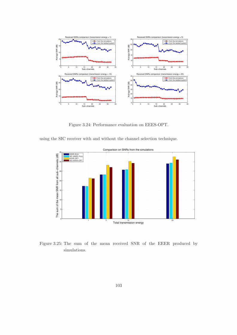
0 5 10 15 20 25 30 350

5

10

15

20

Sub−channels

Avera

ge S

NR

(dB

)

Received SNRs comparison (transmission energy = 1)

from the simulations

from the testbed system

0 5 10 15 20 25 30 355

10

15

20

25

30

Sub−channels

Avera

ge S

NR

(dB

)

Received SNRs comparison (transmission energy = 5)

from the simulations

from the testbed system

0 5 10 15 20 25 30 3510

15

20

25

30

Sub−channels

Avera

ge S

NR

(dB

)

Received SNRs comparison (transmission energy = 10)

from the simulations

from the testbed system

0 5 10 15 20 25 30 3510

15

20

25

30

35

40

Sub−channels

Avera

ge S

NR

(dB

)

Received SNRs comparison (transmission energy = 20)

from the simulations

from the testbed system

Figure 3.24: Performance evaluation on EEES-OPT.

using the SIC receiver with and without the channel selection technique.

1 5 10 200

5

10

15

20

25

30

35

Comparison on SNRs from the simulations

Total transmission energy

The s

um

of th

e m

ean S

NR

fro

m a

ll sub−

channels

(dB

)

EEER−FULL

SIC−EEER−FULL

EEER−OPT

SIC−EEER−OPT

Figure 3.25: The sum of the mean received SNR of the EEER produced by

simulations.

103

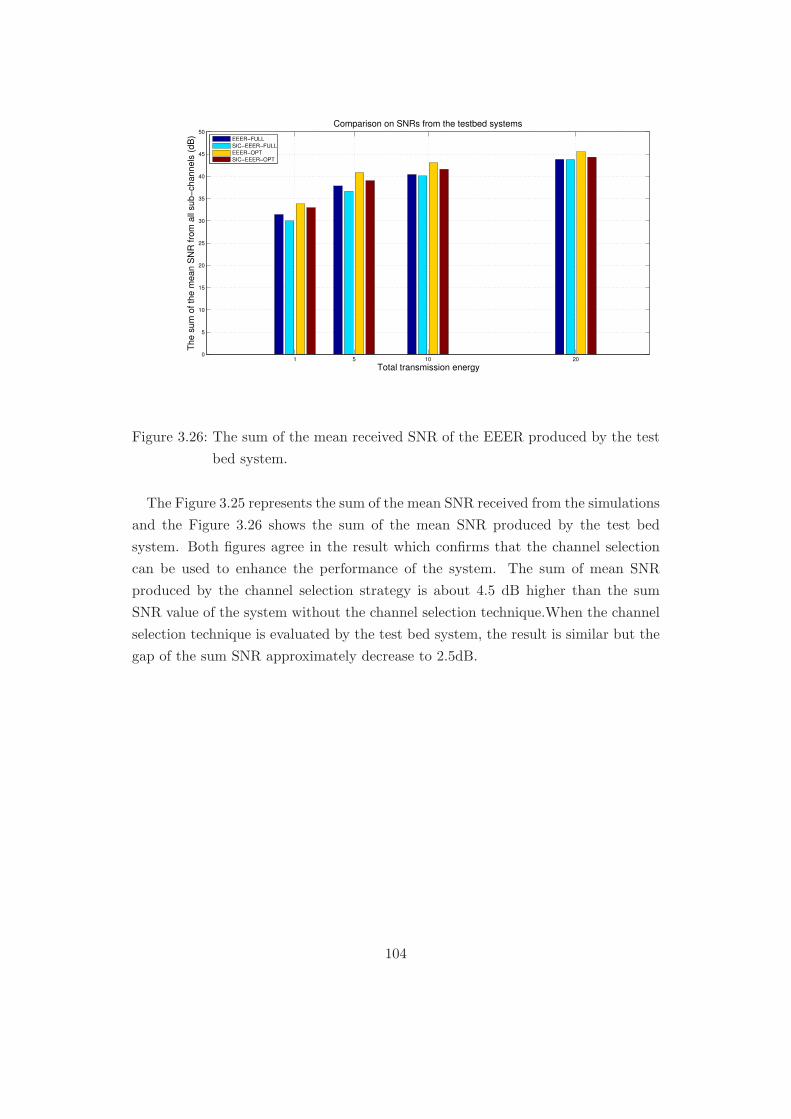
1 5 10 200

5

10

15

20

25

30

35

40

45

50

Comparison on SNRs from the testbed systems

Total transmission energy

The s

um

of th

e m

ean S

NR

fro

m a

ll sub−

channels

(dB

)

EEER−FULL

SIC−EEER−FULL

EEER−OPT

SIC−EEER−OPT

Figure 3.26: The sum of the mean received SNR of the EEER produced by the test

bed system.

The Figure 3.25 represents the sum of the mean SNR received from the simulations

and the Figure 3.26 shows the sum of the mean SNR produced by the test bed

system. Both figures agree in the result which confirms that the channel selection

can be used to enhance the performance of the system. The sum of mean SNR

produced by the channel selection strategy is about 4.5 dB higher than the sum

SNR value of the system without the channel selection technique.When the channel

selection technique is evaluated by the test bed system, the result is similar but the

gap of the sum SNR approximately decrease to 2.5dB.

104

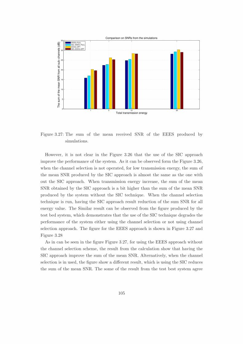
1 5 10 200

5

10

15

20

25

30

35

Comparison on SNRs from the simulations

Total transmission energy

The s

um

of th

e m

ean S

NR

fro

m a

ll sub−

channels

(dB

)

EEES−FULL

SIC−EEES−FULL

EEES−OPT

SIC−EEES−OPT

Figure 3.27: The sum of the mean received SNR of the EEES produced by

simulations.

However, it is not clear in the Figure 3.26 that the use of the SIC approach

improve the performance of the system. As it can be observed form the Figure 3.26,

when the channel selection is not operated, for low transmission energy, the sum of

the mean SNR produced by the SIC approach is almost the same as the one with

out the SIC approach. When transmission energy increase, the sum of the mean

SNR obtained by the SIC approach is a bit higher than the sum of the mean SNR

produced by the system without the SIC technique. When the channel selection

technique is run, having the SIC approach result reduction of the sum SNR for all

energy value. The Similar result can be observed from the figure produced by the

test bed system, which demonstrates that the use of the SIC technique degrades the

performance of the system either using the channel selection or not using channel

selection approach. The figure for the EEES approach is shown in Figure 3.27 and

Figure 3.28

As in can be seen in the figure Figure 3.27, for using the EEES approach without

the channel selection scheme, the result from the calculation show that having the

SIC approach improve the sum of the mean SNR. Alternatively, when the channel

selection is in used, the figure show a different result, which is using the SIC reduces

the sum of the mean SNR. The some of the result from the test best system agree

105

with the figure of the calculation, which show improvement when the SIC technique

is incorporated into EEES with no channel selection scheme. Using the channel

selection with the SIC results decrease in the sum SNR for some transmission energy

value.

1 5 10 200

5

10

15

20

25

30

35

40

45

Comparison on SNRs from the testbed systems

Total transmission energy

The s

um

of th

e m

ean S

NR

fro

m a

ll sub−

channels

(dB

)

EEES−FULL

SIC−EEES−FULL

EEES−OPT

SIC−EEES−OPT

Figure 3.28: The sum of the mean received SNR of the EEES produced by the test

bed system.

There is discrepancy between the result produced by the test bed system, which

is operated on the real-time FPGA transceiver, and the result obtained from the

simulations. Hence, although the simulation result present that the SIC can be

used to enhance the performance of the proposed techniques, evaluation on the real

test system cannot confirm. The difference between the set of results produced by

the simulations and the testbed system may be caused by the the configuration

of the channel emulator or the real characteristic of the wireless channel. Further

investigation on the SIC technique is required to determine the cause of discrepancy.

However, one thing can be confirmed for the proposed technique that is the channel

selection can enhance the performance of the MIMO-HSDPA system. As it is proved

by the test bed system, the channel selection approach, which remove the signature

sequences creating low gain channel, enhance the total received SNR for both EEER

and EEES techniques.

106

3.7 Conclusions

The previous chapter showed that having the high data rate yields improving of the

energy efficient as well as the end-to-end throughput. This chapter has demonstrated

how to improve the physical data rate by using the MIMO-HSDPA approach. The

EEES and EEER resource allocation techniques are incorporated into the MIMO-

HSDPA system, which renders significant increase in the data rate. Moreover, the

SIC technique is used in the receiver to mitigate the effect of the ISI, caused by the

frequency selective channel. Having the SIC technique also simplifies the resource

allocation technique, which reduces the computational cost for the EEES approach.

The main contribution of the chapter is using time and frequency synchronization

approach for setting up the test bed system in order to evaluate the performance of

the resource allocation techniques. In the literature review, synchronization between

the transmitter and the receiver of the test bed system is done by using external

clock signal. The clock signal is used as a reference so that the transmitter and the

receiver can linked and operate the transmission.The time and frequency synchro-

nization technique proposed in this chapter is new and can be used to synchronize the

transmitter and the receiver of the test bed system without requirement of the exter-

nal clock signal source.However, the time and frequency synchronization technique

requires the use of pilot signals, which is redundant information. Using the synchro-

nization method, data packet transmission can be performed correctly, which lead

to setting up the MIMO-HSDPA test bed system using LabVIEW-PXIe machine.

The test bed system is used to evaluate the performance of the EEES and EEER

resource allocation technique with the channel selection and the SIC technique. The

testing results confirm that the channel selection enhance the performance of the

EEER and EEES technique, but for the SIC technique, there is some discrepancy

between the results produced from the simulation and the result obtained from the

test bed system, which needs further investigation.

For the next chapter, using the MIMO transmission actually not only experiencing

a frequency selective channel, the system also encounter a correlated channel due

to the antenna configuration. The correlated channel reduced spatial multiplexing

gain of the MIMO system so that the performance decreases. In order to deal with

the correlated channel,pre-coding techniques are needed. The next chapter will

investigate the use of pre-coding approaches in the MIMO system to enhance the

performance over the correlated channel.

107

4 The Performance Improvement of

the MIMO System Over Correlated

Channels

Over frequency selective channels such as pedestrian A and pedestrian B channels,

the system value approach has demonstrated an effective method which simplifies

the resource allocation as well as maximizing the capacity of the channel. The sys-

tem value approach is used together with the signature sequence ordering algorithm,

which puts the signature sequence in the right order and provides the optimum num-

ber of the used sequences. As a result, the maximum capacity close to the iterative

water filling upper bound can be achieved whilst the computational complexity is

minimized in both EEER and EEES algorithms, since no energy calculation is re-

quired before the rate allocation. In addition, when the iterative energy calculation

is performed for the energy allocation, the use of successive interference cancellation

can simplify the matrix inversion, which minimizes the computational cost of energy

calculation. It has been observed that the SIC-based receiver with both the EEER

and the EEES resource allocation algorithm produces substantially throughput im-

provement on for pedestrian A and pedestrian B channels.

In chapter 4, the large gain of the capacity is achieved by the MIMO transmis-

sion working on a spatial multiplex mode, which assumes that signals traverse over

independent paths of the channel between a transmitter and a receiver. Giving NT

and NR as the number of transmitter antennas and receiver antennas, the spatial

multiplexing gain linearly increases the capacity of the systems as a number n grow,

where n = min(NT , NR). However, in practical systems, fading MIMO channels are

rarely to be independent of each other. The MIMO channels are often spoiled by

environments or antennas configurations, for example insufficient spacing between

antenna arrays make correlated fading on the channels. The impact of antenna cor-

relations were investigated by [88,89], which reported that those spatial correlations

can lead to significantly the performance degradation of the MIMO’s spatial multi-

108

plexing. This includes the performance of the resource allocation algorithms, which

are also reduced by the correlated fading effects.

In order to improve the performance of the system over correlated MIMO channels,

pre-coding schemes can be employed. With the channel information available, the

transmitter can formulate a pre-coding scheme such that the spatial correlation has

fewer effects on the MIMO channel. Consequently, the MIMO communication is

able to take the full advantage of the multiplex gain.

In this chapter, the channel capacity and the performance of the EEER and EEES

algorithm is examined over correlated MIMO channels to demonstrate the effects

of the correlated channels.Then, pre-coding schemes are proposed to deal with the

correlated channel problem. Performance improvement produced by the pre-coding

techniques will be presented to confirm effectiveness of the technique over correlated

channel modelled by the so-called kronecker model.

4.1 The MIMO Correlated Channel Model and The

Channel Capacity

4.1.1 The MIMO Channel Model

It is aforementioned that the spatial multiplexing gain increase proportionally to

the n where n = min(NT , NR). This gain can be achieved only in rich scattering

environments, which offer full rank of the channel matrix, and together with perfect

channel estimation on both transmitter and receiver sides. With this assumption,

the total capacity of MIMO channel can be determined by summing the capacity of

parallel AWGN SISO sub-channels, where the number of the sub-channel is specified

by the rank of the MIMO channel matrix. The rich scattering condition however

rarely happens in the practical system, since the MIMO channel characteristics are

associated with the antenna spatial correlation and statistical channel information

will be required to be estimated by the transmitter and the receiver. Therefore, it

is left an open question to solve how the MIMO channel can be modeled such that

the practical channel characteristics are achieved.

There are many channel models which are described by using various assumptions

with the objective is to achieve realistic MIMO channels. The survey of the MIMO

channel was conducted by [23]. It classified the MIMO channel into 2 categories,

physical models and analytical models. With the physical models, channels are

described by parameters associated with the electromagnetic wave propagation and

109

the use of double-directional propagation model. The physical models do not take

antenna configuration and system bandwidth into account for modeling and they

are very accurate in reproducing radio wave propagation.

Another popular model is the analytical model, which describes the channel im-

pulse response and multi-path by using only mathematical methods, without taking

physical wave propagation into consideration. The analytical model is used for-

mulate the MIMO channel matrices, which are necessary for algorithm designing.

As a result, it is more attractive than the physical model in simulations and ver-

ifications. The analytical model can be categorized into two sub models that are

propagation-motivated models and correlated models.

The propagation-motivated models formulate channels according to parameters

defined by the physical propagations. The models classified in this category, for

instance, are finite scatterer models, which were introduced by [90] and were em-

ployed in [91] to determine the capacity of MIMO multiusers channels. The finite

scatterer model formulates a channel matrix as a function of the limited number

scattering paths, governed by the Direction-of-Departure (DoDs) at a transmitter

and Direction-of-Arrival (DoAs) at a receiver. Similarly, other examples of the

propagation-motivated model are maximum entropy models [92], which use the

knowledge of (DoDs), DoAs and the principle of maximum entropy to construct

reliable channel models.

Alternatively, the correlation-based model which describes the channel matrix

by a spatial correlation matrix can be employed to formulate the MIMO channels.

Having a limited number of antennas at a transmitter and a receiver leads to the

usage of a spatial correlation matrix to formulate a MIMO channel. For a given H

as a channel matrix dimension of NR ×NT , the full correlation matrix is written as

R = Evec(H)vec(H)H

(4.1)

The matrix R is NRNT ×NRNT dimensional matrix which characterises correlations

between all transmit and receive antennas and vec(H) denote the column vector of H

generated by appending the columns of the channel vector H together. In addition

to the correlated-based model, the correlation matrix of the transmitter and the

receiver is completely uncorrelated and can be separated but the coupling between

antennas depends on scattering in the environment. As the correlation matrices is

separable, it is possible to define a transmitter correlation matrix RTx and a receiver

110

correlation matrix RRx such that

RTx = EHHH

, RRx = E

HHH

(4.2)

Both matrices basically depend on antenna configurations which create joint angu-

lar power space around a transmitter antenna panel or a receiver antenna panel.

Channel models which are classified as the correlated-based model are the weichsel-

berger [93] model and the kronecker model [25, 94].

The weichselberger model represents the MIMO channel model that has coupled

power between a transmitter and a receiver. Using the weichselberger model, the

channel model H is given as

H = URx(Ω⊙G)UTTx (4.3)

where Ω is the matrix representing coupling between eigenmode of a transmitter

and a receiver (the unitary matrices), whose dimension is given as NR × NT . The

symbol ⊙ denotes the product of Schur-Hadamard while G is the i.i.d matrix whose

dimension is also equal to NR × NT . The matrices URx and UTTx are unitary

matrices which are respectively determined from the correlation of a transmitter

and a receiver, that are

RTx = UTxΛTxUHTx, RRx = URxΛRxU

HRx (4.4)

As it can be seen, the unitary matrix can be obtained by using the eigenvalue

decomposition so that the weichselberger model is known in another name as the

eigen beam model. For rich scattering environment, the rank of the matrix Λ is equal

to one, which demonstrates that the coupling between all modes is identical. This

is a special case of the weichselberger model where the coupling matrix is written

as Λ = λRxλTTx, where λRx and λT

Tx are a vector formulated from the eigenvalue

of the correlation matrix of a receiver and a transmitter respectively. Once the

rich scattering case is encountered, the weichselberger model can be rewritten as a

Kronecker model.

The kronecker model agrees with the weichselberger model which assumes that the

spatial correlation of a transmitter is separable from a receiver. The full correlation

matrix therefore can be formulated by using a kronecker product as

RH = RTx ⊗RRx (4.5)

111

where the RTx and RRx are obtained from (4.2). Using the kronecker model, the

channel matrix is obtained as

vec(H) = R12Hvec(G) (4.6)

R12H is a square root matrix of the full correlation matrix. For a given RTx and RRx

then channel matrix can be written as

H = R1/2RxGR

1/2Tx (4.7)

The kronecker model is valid only if the condition in corollary 3.2 of [12] is satisfied or

it can be said that the coupling between eigenvector of a transmitter and a receiver is

equal in all power profile. In this chapter we assume that the system is operated on

the rich scattering so that the kronecker model will be used to formulate all MIMO

correlated channels to be used in simulations.

4.1.2 Generating MIMO Correlated Channel Matrices

As it is known, the spatial MIMO multiplexing improves the capacity of the MIMO

systems. However, many researches on the capacity of the MIMO systems have been

demonstrated that the spatial multiplexing gain is actually reduced by the spatial

correlations, which is caused by the scattering of wave propagation in systems. Un-

fortunately, realistic MIMO channels always encounter correlated channels which

include all effects of the spatial correlations. It is therefore essential to formulate

the channel matrix as close as to the realistic channels to provide better analytical

results. Spatially correlated channels can be formulated by employing the spatial

correlation matrix as given in (4.1). The model focused in this chapter is the kro-

necker model generated from (4.5). The kronecker model has been investigated and

to show that, apart from the corollary 3.2 of [12], it is also valid for the system with

the small number of antennas such as 2 x 2 MIMO systems. The kronecker model

hence will be used to produce the spatially correlated channels as seen the following

section.

Assuming that a channel impulse response vector represent multi-path impulse re-

sponse between the receive antenna nthr and the transmit antenna nth

t for

nr = 1 , . . . , NR and nt = 1 , . . . , NT is given as

h(nr,nt) =[h(nr,nt)0 , . . . , h

(nr,nt)l , . . . , h

(nr ,nt)L

]Twhere L is a number of resolvable

paths in the multi-path scenario and l = 0 , . . . , (L−1). A channel correlation matrix

112

for lth path obtained at the mth observation interval is given as Hl(m) ∈ NR×NT ,

where

Hl(m) =

h(1,1)l (m) · · · h

(1,nt)l (m) · · · h

(1,NT )l (m)

... · · · ... · · · ...

h(nr ,1)l (m) · · · h

(nr,nt)l (m) · · · h

(nr,NT )l (m)

... · · · ... · · · ...

h(NR,1)l (m) · · · h

(NR,nt)l (m) · · · h

(NR,NT )l (m)

(4.8)

For simplicity, the variable m is neglected and a column vector represent the channel

is obtained by stacking the vector such that

vec(Hl) =[h(1,1)l , . . . , h

(1,NT )l , . . . , h

(nr,1)l , . . . , h

(nr,NT )l , . . . , h

(NR,1)l , . . . , h

(NR,NT )l

]T

(4.9)

where the vec(Hl) is vec(Hl) ∈ NR×NT . The full correlation matrix

RH ∈ NRNT×NRNT over M sample is now written as a function of vec(Hl(m)),

that is

RH = E

1

M

M∑

m=1

(vec(Hl(m))vec(Hl(m))H

(4.10)

where the expectation is produced only for non-zero entries of h(nr,nt)l . The receive

correlation matrix RRx, which RRx ∈ NR×NR , is obtained as

RRx = E

1

M

M∑

m=1

Hl(m)Hl(m)H

(4.11)

The transmit the correlation matrix RTx is defined as

RTx = E

1

M

M∑

m=1

Hl(m)HHl(m)

(4.12)

where RTx ∈ NT×NT . Using the correlation matrices RTx and RRx, the full

spatiotemporal correlation matrix RH can be calculated as given in 4.5.

Now a tap matrix Htap ∈ NRNT×L containing multi-path components in all

MIMO paths can be construct by gathering the correlated channel vector of each

113

multi-path tap together as follows

Htab =[h(1,1) , . . . , h(1,Nt) , . . . , h(nr,1) , . . . , h(nr,NT ) , . . . , h(NR,1) , . . . , h(NR,NT )

]

(4.13)

The tap matrix can be constructed by using

Htab =1√2CmapV(ap) (4.14)

where ap is a power delay profile vector generated as

ap =[ap0 , . . . , apl , . . . , apL

]T ∈ L. The matrix V ∈ NTNR×L is formulated

such that each element has a Rayleigh-distribution amplitudes and a uniformly dis-

tributed phase. The entries of V matrix is generated as independent and identically

distribution (i.i.d) by using circular symmetric complex Gaussian random generator

with zero mean and unity variance CN (0, 1). For simplicity, it can be said that

each column of V is generated as a complex vector Z = (X + jY ), where X and Y

are column vectors of length L and with elements obtained from a i.i.d N (0, σ2/2)

generator. The mapping matrix Cmap ∈ NRNT×NRNT is calculated from

RH = CmapCHmap (4.15)

The matrix Cmap is a square root lower-triangular matrix which can be formulated

by using classic LDL Cholesky decomposition, which is

A = LLH = LDLH = LD12 (LD

12 )H (4.16)

Where L and D is matrices containing eigen vectors and eigen values of the matrix

A respectively. As it can be seen, the full correlation matrix RH is separable and is

obtained from the kronecker product of a transmitter correlation matrix RTx and a

receiver correlation matrix RRx. Consequently, to achieve realistic MIMO channel,

RTx and RRx have to be formulated accordingly.

4.1.3 Calculating Correlation Coefficients for the MIMO Systems

For 2 x 2 MIMO systems, a receives and a transmitter correlation matrix can be

represent by 2 x 2 dimensional matrix, which is

RRx =

[1 r∗

r 1

], RTx

[1 t∗

t 1

](4.17)

114

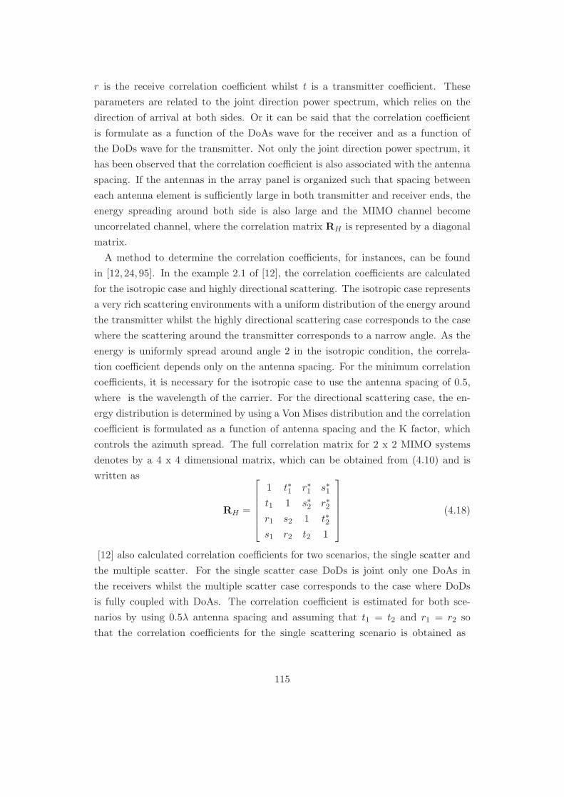
r is the receive correlation coefficient whilst t is a transmitter coefficient. These

parameters are related to the joint direction power spectrum, which relies on the

direction of arrival at both sides. Or it can be said that the correlation coefficient

is formulate as a function of the DoAs wave for the receiver and as a function of

the DoDs wave for the transmitter. Not only the joint direction power spectrum, it

has been observed that the correlation coefficient is also associated with the antenna

spacing. If the antennas in the array panel is organized such that spacing between

each antenna element is sufficiently large in both transmitter and receiver ends, the

energy spreading around both side is also large and the MIMO channel become

uncorrelated channel, where the correlation matrix RH is represented by a diagonal

matrix.

A method to determine the correlation coefficients, for instances, can be found

in [12, 24, 95]. In the example 2.1 of [12], the correlation coefficients are calculated

for the isotropic case and highly directional scattering. The isotropic case represents

a very rich scattering environments with a uniform distribution of the energy around

the transmitter whilst the highly directional scattering case corresponds to the case

where the scattering around the transmitter corresponds to a narrow angle. As the

energy is uniformly spread around angle 2 in the isotropic condition, the correla-

tion coefficient depends only on the antenna spacing. For the minimum correlation

coefficients, it is necessary for the isotropic case to use the antenna spacing of 0.5,

where is the wavelength of the carrier. For the directional scattering case, the en-

ergy distribution is determined by using a Von Mises distribution and the correlation

coefficient is formulated as a function of antenna spacing and the K factor, which

controls the azimuth spread. The full correlation matrix for 2 x 2 MIMO systems

denotes by a 4 x 4 dimensional matrix, which can be obtained from (4.10) and is

written as

RH =

1 t∗1 r∗1 s∗1

t1 1 s∗2 r∗2

r1 s2 1 t∗2

s1 r2 t2 1

(4.18)

[12] also calculated correlation coefficients for two scenarios, the single scatter and

the multiple scatter. For the single scatter case DoDs is joint only one DoAs in

the receivers whilst the multiple scatter case corresponds to the case where DoDs

is fully coupled with DoAs. The correlation coefficient is estimated for both sce-

narios by using 0.5λ antenna spacing and assuming that t1 = t2 and r1 = r2 so

that the correlation coefficients for the single scattering scenario is obtained as

115

t = 0.03 − j0.2, r = −0.4 + j0.33, s1 = −0.19 + j0.21 and s2 = 0.56 + j0.03.

For the multiple scattering scenario, the correlation coefficients are calculated as

t = 0.03− j0.2, r = −0.4+ j0.33, s1 = rt = 0.05+ j0.09and s2 = rt∗ = −0.08− j0.07

If the kronecker model is employed, it can be seen that both scenario are identi-

cal full correlation matrices. However, it is suggest the only the direction scatter

scenario is accurate according to the separability assumption in the proposition 3.2

of [12], the kronecker model is valid only if DoDs couple with the same power profile

into all DoAs, and vice versa, or demonstrated the multiple scattering scenario.

[24] was simplified the spatial correlation model for Indoor IEEE 802.11n sys-

tems. This work employs Saleh-Valenzuela [96] correlation-based model which de-

scribes the multipath components departures and arrivals at an observation point as

clusters. The Lapacian distribution is used to describe the energy spreading around

the antenna and to formulate an equation to determine the correlation coefficient.

This is done as a function of three parameters, direction of angle, angular spread

and antenna spacing.

The study in [95] proposes a deterministic MIMO channel model for the outdoor

to indoor environments. The channel models have been developed as a Tapped De-

lay Line (TDL) model for broadband fixed wireless systems by using a measurement

based methods. In this work the models are formulated for two types of indoor envi-

ronments, closed and open scenarios. The closed scenario represents systems where

a large number of scatters are close to a receiver, such as small offices or laboratories,

whilst the open scenario such as large class rooms perform environments with few

scatters. The models have been examined and compared with values obtained from

measurements and they are found to be accurate for using in simulations.

Having the correlation matrix correlated mapping matrix can be obtain from

(4.15) and the MIMO correlated channel impulse response can be formed by using

(4.14). The channel impulse response is employed to form the correlated channel

for the MIMO systems to be examined for the capacity as discussion in the next

section.

4.2 The Capacity of the MIMO channel

The use of multiple antennas at a receiver and a transmitter provides a spatial

multiplexing gain which offers a linearly increase in the spectral efficiency. This is a

significant improvement when compared with the contemporary systems where the

increase in spectral efficiency and capacity is shown in a logarithm scale. However,

116

this is based on rich scattering environments where MIMO channels are uncorrelated.

Correlated channels certainly degrade the spectral efficiency and, for high correlation

channels, the system might be converted to a SISO system which does not provide

any system gains. A tutorial of the capacity of MIMO systems was conducted by [97],

which derived the mean capacity of a complex AWGN MIMO channel as

C = E

log2

[det(TNR

+ρ

NTHHH)

](4.19)

Where ρ is an average SNR per receiver antennas. The product of HHH can be

written by using Singular Value Decomposition (SVD), which rewrite the channel

matrix as

H = UΣVH (4.20)

Where U and V are unitary matrices of left and right of singular vector respectively.

Σ is a diagonal matrix whose main diagonal contains singular values. By using the

SVD approach, the capacity is given as

C = E

log2

[det(TNR

+ρ

NTUΣΣHUH)

](4.21)

The capacity of MIMO system is equal to the summation of the AWGN SISO sub-

channels as given in (4.21), where the number of sub-channels is obtained as the

rank of the channel matrix, determined as

rank(H) = k ≤ min NR, NT (4.22)

The capacity now can be obtained as

C = E

k∑

i=1

log2(1 +ρ

NTσ2i )

(4.23)

Where σ2i are the square singular of the diagonal matrix

∑. The upper bound of

the a Rayleigh fading MIMO channel is obtained as

C = E

NT × log2(1 +

ρ

NTχ22NR

)

(4.24)

χ22NR

represents a chi-distributed random variable with 2NR degree of freedom. The

upper bound can be achieved when each of the NT transmitted signals is received

by the same set of NR antennas without interference.

117

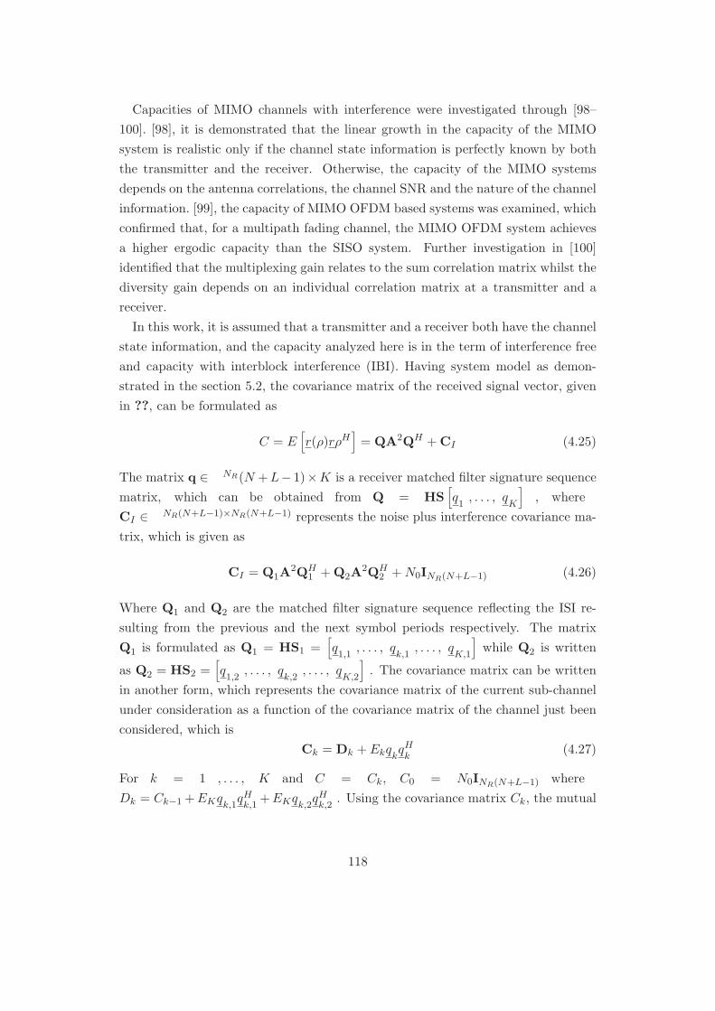
Capacities of MIMO channels with interference were investigated through [98–

100]. [98], it is demonstrated that the linear growth in the capacity of the MIMO

system is realistic only if the channel state information is perfectly known by both

the transmitter and the receiver. Otherwise, the capacity of the MIMO systems

depends on the antenna correlations, the channel SNR and the nature of the channel

information. [99], the capacity of MIMO OFDM based systems was examined, which

confirmed that, for a multipath fading channel, the MIMO OFDM system achieves

a higher ergodic capacity than the SISO system. Further investigation in [100]

identified that the multiplexing gain relates to the sum correlation matrix whilst the

diversity gain depends on an individual correlation matrix at a transmitter and a

receiver.

In this work, it is assumed that a transmitter and a receiver both have the channel

state information, and the capacity analyzed here is in the term of interference free

and capacity with interblock interference (IBI). Having system model as demon-

strated in the section 5.2, the covariance matrix of the received signal vector, given

in ??, can be formulated as

C = E[r(ρ)rρH

]= QA2QH + CI (4.25)

The matrix q ∈ NR(N +L− 1)×K is a receiver matched filter signature sequence

matrix, which can be obtained from Q = HS[q1, . . . , q

K

], where

CI ∈ NR(N+L−1)×NR(N+L−1) represents the noise plus interference covariance ma-

trix, which is given as

CI = Q1A2QH

1 + Q2A2QH

2 + N0INR(N+L−1) (4.26)

Where Q1 and Q2 are the matched filter signature sequence reflecting the ISI re-

sulting from the previous and the next symbol periods respectively. The matrix

Q1 is formulated as Q1 = HS1 =[q1,1

, . . . , qk,1

, . . . , qK,1

]while Q2 is written

as Q2 = HS2 =[q1,2

, . . . , qk,2

, . . . , qK,2

]. The covariance matrix can be written

in another form, which represents the covariance matrix of the current sub-channel

under consideration as a function of the covariance matrix of the channel just been

considered, which is

Ck = Dk + EkqkqHk

(4.27)

For k = 1 , . . . , K and C = Ck, C0 = N0INR(N+L−1) where

Dk = Ck−1 +EKqk,1

qHk,1

+EKqk,2

qHk,2

. Using the covariance matrix Ck, the mutual

118

information is given as

I = log2

[det(QA2QH

]− log2 [detCI ]

= log2

[det(INR(N+L−1) + C−1

I QQ2QH)] (4.28)

The mutual information is then exploited to estimate both the capacity of the inter-

block-interference (IBI) free system and the capacity of system with the IBI as

4.2.1 The Capacity for the Case with IBI

Under the assumption that IBI exists, the spatiotemporal MIMO channel H1 and

H2 is not zero. The covariance interference matrix given in (4.26) can be used to

calculate the capacity of the IBI system (CIBI) such that

CIBI =1

Nlog2

[det(INR(N+L−1) + C−1

I QA2QH)]

(4.29)

where the definition of det(I+AB) = det(I+BA) is used in the capacity formulation.

The capacity of the system calculated from (4.29) is given in bits/chip.

4.2.2 The Capacity for the IBI Free Case

Under the assumption of no IBI, the spatiotemporal MIMO channel matrices H1

and H2 are set to be H1 = H2 = 0. The covariance matrix hence is given by

C = E[r(ρ)r(ρ)H

]= QA2QH + N0INR(N+L−1) (4.30)

As the interference covariance matrix is reduced to CI = N0INR(N+L−1) so that the

inversion of the covariance matrix therefore written as CI = 1N0

INR(N+L−1). The

channel capacity of the matrix H and the given spreading sequence can be then

given in term if bits per chip as

CST =1

Nlog2

[det(INR(N+L−1 +

1

N0SHHHHSA2)

](4.31)

Where the definition of det(I + AB) = det(I + BA) is also applied on (4.31).

119

4.3 Minimizing the Effect of the MIMO Correlated

Channels Using a Pre-Coding Approach

A MIMO technique will be required to improve when operating the system in a

rich scatter environment. In practical systems channel correlations are unavoidable

but the effect of the channel can be reduced by using pre-coding techniques at the

transmitter. With the channel state information available at the transmitter, the

pre-coding scheme can be formulated such that it modifies the information to be

transmitted to match the channel conditions, to significantly improve the perfor-

mance at the receiver.

There are many criteria for designing the pre-coding, for example maximizing er-

godic or received signal-to-noise ratio or minimizing bit-error-rate at the receivers

[100], and designing of the pre-coding scheme depending on how the Channel State

Information (CSI) is available to the transmitter. The impact of the CSI on the

performance of the systems was investigated in [101], which demonstrated that the

capacity is reduced as the availability of the CSI decreases. When the CSI is perfectly

known by a transmitter, the optimal pre-coding scheme such as a linear pre-coding

might be used to improve the performance. The linear pre-coding is a linear trans-

formation that can map information bits to coded bits by a pre-coding block. The

linear pre-coding can also be employed in the partial CSI condition, but perfor-

mance degrades. Work [101] also proposed how to optimize the linear pre-coder

for different CSI criteria. The best pre-coding scheme which is used when CSI is

available at both transmitter and receiver is the singular value decomposition (SVD)

approach [102, 103]. For a given of received signal vector y ∈ NR as y = Hx + n,

where x ∈ NR × NT is a transmitted signal vector and the vector n is a com-

plex Gaussian noise with zero mean and the variance is set to be equal to one in

both real and imaginary part. When using the SVD approach, the channel matrix

H ∈ NR ×NT , can be partitioned into three components, that are U and V which

are known as left and right unitary matrices and Σ, the diagonal matrix of singular

values of the matrix H, as shown in (4.20). Therefore, the transmitted signal vector

x can be multiplied with V, which is known as a pre-coding matrix, whilst, at the

receiver, a received signal vector y might be multiplied by UH , a receiver filter, such

that

y = UH(HVx + n) = Σx + n (4.32)

where n = UHn is also the complex Gaussian noise. Since the Σ is the diagonal

120

matrix, the MIMO channel is separated in to sub SISO channels with different gains,

and the number of sub channels is determined by the rank of the channel matrix

H. Another pre-coder method is zero-forcing (ZF) or minimum-mean-square-error

(MMSE) algorithm that is based on the inverse of the channel matrix. This method

has been used in the multi-user context as described in [104–106]. Giving W as a

pre-coding matrix for the multi-user system, the ZF pre-coding matrix is given as

W = HH(HHH)−1 (4.33)

Further improvement of the ZF pre-coding can be achieved by including a regularized

factor in the equation, which is

W = HH(HHH + βI)−1 (4.34)

Where β denotes a regularized factor, which determines interference level in the

multi-users system. For β > 0, The system is corrupted by the interference. Basi-

cally, the β is chosen such that received SNR is maximized. Given in (4.34), it is

also known as the MMSE pre-coding scheme, whose performance is good at very low

SNR. For the high SNR region, the performance of the MMSE pre-coding approach

is the same as the ZF pre-coder.

There are two pre-coding schemes to be investigated in this work, the Eigen vec-

tor pre-coding and the inverse channel pre-coding. Both approaches are employed

in collaboration with the resource allocation schemes that have been discussed in

Chapter 3, EEER and EEES approach, in order to observe the performance over

the correlated channels.

4.3.1 The Eigen-Vector Pre-Coding Approach

It assumes that the MIMO channel matrix H is a full rank matrix and the maximum

number of spreading sequences as K = NTN . The Eigen value of HHH is obtained

as σ2k for k ∈ 1 , . . . , K. In addition to the Eigen value, they are assumed to be

satisfy the condition that σ2k > σ2

k−1 for all k. The channel covariance matrix can

be separated by using Eigen value decomposition, which represents the covariance

matrix of the channel in term of a matrix of Eigen Vectors and a diagonal matrix of

the Eigen values as

HHH = UΛUH (4.35)

121

where U ∈ (NTN)×(NTN) is a unitary matrix of Eigen vectors where satisfies

UHU = INTN , and Λ ∈ (NTN)×(NTN) = diag(σ21 , . . . , σ2

k, . . . , σ2NTN ) is a diagonal

matrix of Eigen values of HHH. If the signature sequence matrix S is selected such

that S = U, each signature sequence is normalized to have unity average energy,

which is |sk|2 = 1 for k = 1 , . . . , K. With the Eigen value pre-coding approach,

received symbols are still obtained as shown in (3.14). If energy allocated into the

kth channel is given as and the IBI is not considered, the IBI free capacity is written

as

CST =1

N

K∑

k=1

log2(1 +Ekσ

2k

N0) (4.36)

which is given in bits/chip. If the IBI is taken into consideration, the capacity of

the system is determined from (4.29) instead.

4.3.2 The Inverse Channel Pre-Coding Approach

For NT = NR, a zero forcing or an MMSE pre-coder can be used. The ZF pre-coder

is constructed as

B = HHB (HBH

HB )−1 ∈ (NTN)×(NTN) (4.37)

The MMSE pre-coding is given as

B = HHB (HBH

HB +

N0NT

EcI(NRN)×(NRN))

−1 ∈ (NTN)×(NTN) (4.38)

The per-coder spatiotemporal channel convolution matrix HB ∈ (NTN)× (NTN)is

constructed by using a truncation matrix TB =[IN 0N×(L−1)

]∈ N×(N+L−1) to

truncate the MIMO channel convolution matrix given in (3.12) using the relationship

H(nr,nt)B = TBH

(nr,nt) (4.39)

The truncation matrix TB is used to adjust the dimension of the channel other-

wise the channel matrix cannot match the pre-coding matrix.The truncated MIMO

channel convolution matrix is then formulated using

HB =

H(B1, 1) · · · H

(B1, NT )

.... . .

...

H(BNR, 1) · · · H

(BNR, NT )

(4.40)

122

The trace of the covariance matrix of the pre-coding is set to be NTN by using

a normalized vector = diag(BHB) = [v21 , . . . , v2NRN ]T and normalizing the pre-

coding matrix using B = Bdiag( 1v1

, . . . , 1vNRN

). The transmit vector is formulated

as

zB =[zTB,1 , . . . , zTB,nt

, . . . , zTB,Nt

]T∈ NTN (4.41)

and it is produced by using zB(ρ) = BSAy(ρ) at the output of the pre-coder. If

the signature sequence is not used at the transmitter, symbols to be transmitted

are spread by the pre-coding instead. Hence, S = B and the transmit vector is

form as zB(ρ) = BAy(ρ). The receiver signal vector at the output of the chip

matched filter is given by a block of chip matched filter signal samples r(ρ) =[zTB,1 , . . . , zTB,nt

, . . . , zTB,Nt

]T∈ NR(N+L−1) as

r(ρ) = HzB(ρ) + H1zB(ρ− 1) + H2zB(ρ− 2) + n(ρ) (4.42)

Where n ∈ NR(N+L−1)is a complex Gaussian noise vector. The matched filter re-

ceiving spreading sequence for the pre-coder system is constructed using QB = HBS

and the corresponding ISI matrices are given by

QB,1 = H1BS =[q1,1

, . . . , qk,1

, . . . , qK,1

]and

QB,2 = H2BS =[q1,2

, . . . , qk,2

, . . . , qK,2

]. The interference covariance matrix

for the inverse channel pre-coding approach is given by

CI = QB,1A2QH

B,1 + QB,2A2QH

B,2 + N0INR(N+L−1) (4.43)

The capacity of the pre-coding system can then be calculated using the covariance

matrix and the equation (4.29).

For the MMSE receiver with successive interference cancellation (SIC) and the

MMSE receiver without the SIC, the system uses the structure described in the

chapter 3. The total system capacity for the MMSE receivers for both the non-SIC

and SIC based receiver are given as

CSV =1

N

K∑

k=1

log2(1 +λk

Γ(1 − λk)) (4.44)

where λk is a system value determined for the kth channel and Γ represents a system

gap value. The detail of the system value and the system gap value is also given in

the chapter 4.

123

4.4 Performance evaluations using simulations

This chapter aims to solve the correlated channel problem, which reduces the spatial

multiplexing gain of the MIMO system and the performance of the proposed resource

allocation schemes, EEES and EEER, by using pre-coding approaches. The pre-

coding schemes which are going to be investigated are Eigen vector pre-coder, zero-

forcing (ZF) pre-coder and the minimum-mean-square-Error (MMSE) pre-coder.

As described in chapter 3, the EEES stands for equal-energy-equal-SNR. The

EEES approach allocates data rate by using the mean system value, which produce

the capacity close to the water filling iterative water filling upper bound. Then, the

energy is allocated to each channel such that SNR at output of the MMSE receiver

is identical in all channels. This is to ensure that each is loaded with sufficient

energy so that data rate allocated by the transmitter can be achieved by receiver as

well. However, to make the received SNR equally, the EEES requires an iterative

calculation for the energy loading, which is computationally expensive. The EEER

is simpler than the EEES as no iterative energy calculation is required, but the total

data rate achieved by the receiver is low. This is because only the minimum data are

allocated equally to each channel in order to ensure that the data rate satisfy match

to the allocated energy. The EEER employs the minimum system value approach

in the bit allocation. It has been demonstrated that the computation cost of the

EEER is low but the system capacity is reduced.

The pre-coders schemes are incorporated into the resource allocation schemes

when operating over the correlated pedestrian A MIMO channels which are pro-

duced using made to be correlated channels by the well-known kronecker model, as

described in section 5.1.2. There are three scenarios to be simulated and these sce-

narios specify the correlation matrices, which are employed by the kronecker model

to create correlated MIMO channels corresponding to each scenario.

The first scenario is taken from example 3.1 in [12], which represents an outdoor

system. There are three DODs given as θt,1 = π/6, θt,2 = π/2 and θt,3 = 2π/3

whilst the DOAs are given as θr,1 = π/4, θr,2 = π/3 and θr,3 = 3π/4. The com-

plex Gaussian statistic is used to describe the scattering mechanism and the an-

tenna spacing is set to λ2. The transmitter correlation coefficients is calculated as

t ∼= 13

∑3l=1 exp(−jπ cos θt,l) = 0.03 − j0.2 where the receiver correlation coefficients

is obtained as r ∼= 13

∑3l=1 exp(−jπ cos θr,l) = −0.4−j0.33 . Having these correlation

124

coefficients, the correlation matrices is formulated as

Rt =

[1 0.03 + j0.2

0.03 − j0.2 1

], Rr =

[1 −0.4 + j0.33

−0.4 − j0.33 1

]

(4.45)

Hence, the full correlation matrix giving by (4.5) is written as

R =

1 0.03 + j0.2 −0.4 + j0.33 −0.078 − j0.0701

0.03 − j0.2 1 0.054 + j0.0899 −0.4 + j0.33

−0.4 + j0.33 0.054 − j0.0899 1 0.03 + j0.2

−0.078 − j0.0701 −0.4 − j0.33 0.03 − j0.2 1

(4.46)

The second and the third scenarios are taken from [95], which models the channel for

MIMO broadband fixed wireless systems. Both scenarios are called closed scenario

and open scenario respectively and they represents the outdoor to indoor environ-

ments. The closed scenario is referred to indoor environment where the scattering

objects are placed very close to the receiver whilst the open scenario is an indoor

environment where a few scattering object is located near the receiver. It might

be considered that the closed environment is connected to an environment such as

small offices or laboratories and the open environment corresponds to an environ-

ment such as large classrooms or assembly rooms. The correlation matrices for both

scenarios is obtained by measurement based methods, which are given as

Ropen =

1 0.73 0.84 0.64

0.73 1 0.70 0.83

0.84 0.70 1 0.74

0.64 0.83 0.74 1

, Rclosed =

1 0.71 0.93 0.72

0.71 1 0.69 0.92

0.93 0.69 1 0.72

0.72 0.92 0.72 1

(4.47)

The simulations are also performed on Matlab using the 2 x 2 MIMO system model

as describing in section 5.2. The results are produced as an average capacity over

correlated pedestrian A channels. Firstly, the effect of each scenario on the IBI

free capacity and IBI capacity will be investigated, both capacities are calculated

using (4.31) and (4.29). Then, the effect of the correlated channel on each resource

allocation scheme will be analyzed. The results are given as the Figure 4.1.

It has been demonstrated that the worst performance is obtained in the closed

environments, which requires 7 dB more SNR input than the case corresponding to

the uncorrelated channel to produce the same capacity, measured in the linear region

125

Figure 4.1: The average capacity A.IBI free channels B.IBI channels

in both IBI and IBI free channel. The highest capacity is obtained in the outdoor

environment, which required 3 dB less to achieve the same capacity comparing with

the closed scenario. For the open scenario, the capacity is slightly better than the

closed scenario, the required SNR input is about 1 dB better. Next, the performance

of resource allocation approaches the pre-coding approach will be evaluated.

When the technique is operated, the signature sequences creating bad channels,

which are low gain channels, are removed so that energy is allocated only to good

channels which yields the maximum capacity, as it can be seen in the Figure 4.2a.

The approach with the optimal signature sequence is labeled by OPT whilst the

implementation of a full number of the signature sequences is given under FULL.

The equal-energy-equal-SNR with optimal signature sequence (EEES-OPT) selec-

tion produces the highest capacity and it actually can be observed that the signature

sequence selection improves the performance of the EEES and EEER resource al-

location schemes. Using the low gain channels in the low SNR input region is not

effective, since it consumes too much energy. Removing those channels optimizes

the energy consumption so that the channel selection approach outperforms the full

channel implementation in the low SNR input. The performance of the successive

interference cancellation (SIC) is demonstrated in the Figure 4.2b. It can be seen

that the SIC improves the capacity for all the resource allocation schemes. The SIC

126

Figure 4.2: The performance evaluation of A.The channel selection approach B.TheSIC receiver structure

approach will be used as the based technique, when analysing the performance of

pre-coding systems.

Figure 4.3 compares the average capacity of the correlated channel defined by each

scenario. Note that, the capacity curves are produced from averaging the capacity

over 50 pedestrian A channels, where each channel is generated to be a correlated

channel by using the kronecker model and the correlation matrices specified by each

environment. As it can be seen, there is a bit fluctuation caused by the correlated

channels. The capacity curve produced over the outdoor environment give the high-

est value in all resource allocation approaches. The results agrees with the one

demonstrated by Figure 4.1, where the outdoor environment achieves the highest

capacity. Next the performance of the pre-coding techniques will be identified.

Figure 4.4 shows the results of using pre-coders with the EEES approach on the

outdoor channel and the results on the open scenario and on the close scenario are

respectively given by figure 3.8 and 3.9. In the Figure 4.4 a, The capacity of

CIBI and CST are given in (4.29) and (4.31) and they are produced by equal energy

loading in all multi-code channels. The Eigen vector pre-coding is for the EEES

approach is labelled by EIG whilst the MMSE pre-coding approach and the zero-

forcing pre-coding approach is named using prefix MMSE and ZF respectively. The

Eigen vector pre-coder is obtained as (4.35), which employs the pre-coding matrix

127

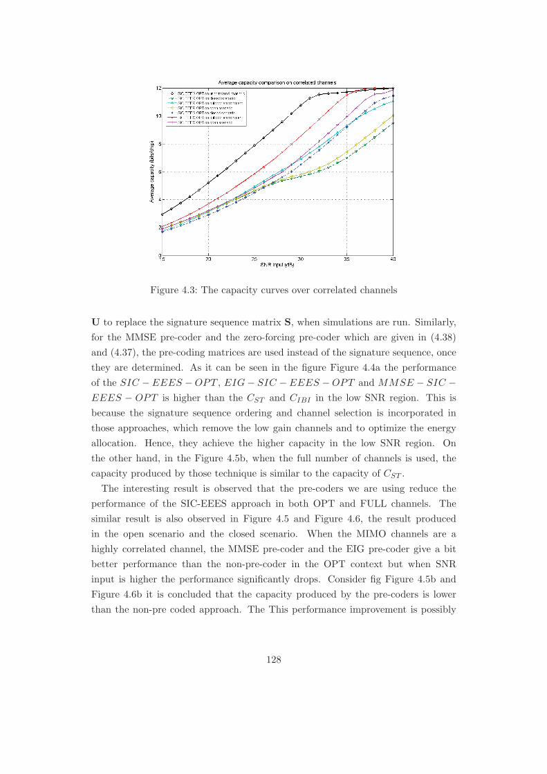
Figure 4.3: The capacity curves over correlated channels

U to replace the signature sequence matrix S, when simulations are run. Similarly,

for the MMSE pre-coder and the zero-forcing pre-coder which are given in (4.38)

and (4.37), the pre-coding matrices are used instead of the signature sequence, once

they are determined. As it can be seen in the figure Figure 4.4a the performance

of the SIC −EEES −OPT , EIG− SIC −EEES −OPT and MMSE − SIC −EEES − OPT is higher than the CST and CIBI in the low SNR region. This is

because the signature sequence ordering and channel selection is incorporated in

those approaches, which remove the low gain channels and to optimize the energy

allocation. Hence, they achieve the higher capacity in the low SNR region. On

the other hand, in the Figure 4.5b, when the full number of channels is used, the

capacity produced by those technique is similar to the capacity of CST .

The interesting result is observed that the pre-coders we are using reduce the

performance of the SIC-EEES approach in both OPT and FULL channels. The

similar result is also observed in Figure 4.5 and Figure 4.6, the result produced

in the open scenario and the closed scenario. When the MIMO channels are a

highly correlated channel, the MMSE pre-coder and the EIG pre-coder give a bit

better performance than the non-pre-coder in the OPT context but when SNR

input is higher the performance significantly drops. Consider fig Figure 4.5b and

Figure 4.6b it is concluded that the capacity produced by the pre-coders is lower

than the non-pre coded approach. The This performance improvement is possibly

128

Figure 4.4: The Average capacity of pre-coding system on outdoor environment A.with SIC-EEES-OPT B. with SIC-EEES-FULL

not from the pre-coders but the channel selection technique. The reason that the

pre-coding approach can not improve the performance of the system may come from

the formulation of the pre-coder. Currently, the pre-coder is formulated by using the

information of the channel matrix considered as a correlated channel. The channel

matrix generated from the kronnecker model may be not accurate enough and need

to investigate in order to achieve the right result.

For the results of SIC-EEER, they are giving in Figure 4.7, 4.8 and 4.9. The

results for the EEER with channel selection agree with the EEES approach, which

confirms that the pre-coding scheme does not provide any improvement when the

low gain channels are discarded. Simulations on EEER with full channel imple-

mentation produce other distinct results, which have shown that using the MMSE

pre-coder achieve the best performance. The EEER approach produces the data

rate allocation using the minimum system value approach. As the MMSE pre-coder

produces the highest capacity, this means the MMSE pre-coder improves the min-

imum system values. The performance of the EIG pre-coder is dropped below the

performance of the ZF pre-coder. This suggests that the EIG pre-coding scheme is

not suitable for the EEER with full channel implementation. The reason why the

MMSE pre-coding improve only the minimum system value is not clear. It might

has effect on the low gain channel but not the high gain channel and, by this using

129

Figure 4.5: The Average capacity of pre-coding system on open scenario A. withSIC-EEES-OPT B. with SIC-EEES-FULL

assumption, the only minimum system vale is enhanced. The performance of the

pre-coding need more investigation in the future works.

4.5 Conclusions

In this chapter, the effects of correlated MIMO channels caused by antenna config-

urations and system environments have been analysed by simulation methods. In

order to run the simulations, the so-call kronecker model is employed with realis-

tic correlation matrices to generated MIMO correlated channels. Then, the EEES,

EEVR and EEER resource allocation approach have been tested on the formulated

channel to evaluate the performance and simulation confirms that the MIMO cor-

related channel degrade the performance of the proposed resource allocations. In

order to improve the performance over the correlated channel, pre-coding approach

is employed. There are three pre-coding techniques to be examined, that are the

Eigen vector pre-coding, the channel inverse MMSE pre-coding and the channel in-

verse zero forcing pre-coding. These pre-coding approaches are incorporated into

the resource allocation techniques to produce simulation results. From the simula-

tions, it has been observed that these pre-coding approaches are unable to improve

the performance over the correlated channels and only the signature sequences or-

130

Figure 4.6: The Average capacity of pre-coding system on close scenario A. withSIC-EEES-OPT B. with SIC-EEES-FULL

dering and the channel selection technique is able to produce the best performance.

For further improvement, the pre-coding still is a favorite for solving the correlated

channels problem but it needs to be redesigned such that the effects of correlated

channel are minimized.

131

Figure 4.7: The Average capacity of pre-coding system on outdoor environment A.with SIC-EEER-OPT B. with SIC-EEER-FULL

Figure 4.8: The Average capacity of pre-coding system on open scenario A. withSIC-EEER-OPT B. with SIC-EEER-FULL

132

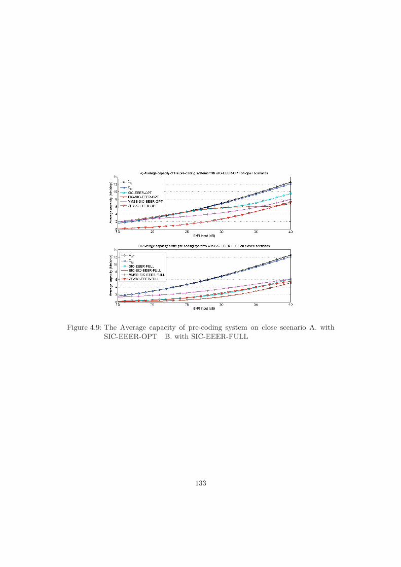
Figure 4.9: The Average capacity of pre-coding system on close scenario A. withSIC-EEER-OPT B. with SIC-EEER-FULL

133

5 Summary and future work

5.1 The summary of the thesis

The thesis focuses on the improvement of the performance of wireless networks,

which mainly concentrates on ad hoc networks. The objective of the first technical

chapter is to obtain the energy efficiency and maximizing end-to-end throughput for

the networks, which can be achieved by using a cross layer optimization approach.

The ad hoc network is assumed to be a stationary network so that the small scale

fading has low effects on the channel. Hence the channel can be assumed as a flat

fading channel. To optimize the throughput, the physical layer of the network is

improved by using the HSDPA technique with the two group resource allocation ap-

proach. The two group technique employs residual energy to enhance the physical

data rate. As a result, the downlink throughput and the energy efficiency are signif-

icantly enhanced. At the routing layer, a multipath routing with a load balancing

algorithm is exploited for further improvement. The multi-path routing employs

the trellis-hop with the modified Viterbi algorithm to identify a set of disjoint paths

which consume minimum energy to deliver data packets. To discover the minimum

energy consumption paths, the routing algorithm uses the bit-energy consumption

which is formulated in conjunction with the link data rate as a cost metric. Using

the bit-energy consumption ensures the system achieve more energy efficiency whilst

using the trellis-hop with the modified Viterbi algorithm minimize the complexity

in paths searching. In addition to energy efficiency improvement, the load balancing

algorithm which distributes data traffic over the multiple data routes is used. The

load balancing approach spread data such that the energy consumed by each data

path is uniform, which results the extension of the network life time and the higher

energy efficiency.

The problem to be solved in the chapter is to maximize the end-to-end throughput

of the networks where the flat fading channel is presence. The proposed solution is

to use the packet size optimization as specified by (2.3). It can be seen that the MAC

service time is required in order to obtain the packet size so that the contribution

134

in this chapter is to determine the service time which maximize the end-to-end

throughput. The simplified Cavalho’s service time model which is modified from the

original is employed to determine the service time for the optimal packet size. The

simulation results has shown that the modified service time model can produced

the accurate service time when compared with the service time given by the NS-2

simulation. When using the simplified service time model the packet size which

maximize the throughput can be obtained.

Analysis on the service time has shown that the service time is inversely propor-

tional to the physical data rate. However, the service timer also connects to the

end-to-end throughput by the inverse relationship. This shows the potential further

improvement for the end-to-end throughput by increasing the data rate. The prob-

lem leads to the next chapter which shows the improvement of the physical data

rate of the wireless systems by using a MIMO transmission technique. When the

data rate is increased, the channel is changed to a frequency selective channel so

that this chapter shows how to optimize the data rate and the downlink through-

put for the MIMO transmission system when operating over the frequency selective

channel. In order to maximize the data rate two resource allocation schemes based

on the system value optimization have been proposed. The first scheme is called the

Equal-Energy-Equal-SNR (EEES), which allocate the data rate by using the mean

system value. Using the EEES approach provides a significant enhancement in the

data rate but it requires iterative energy calculation in the energy allocation. As

a result, the computation complexity is higher. Alternatively, the Equal-Energy-

Equal-Rate can (EEER) be employed, if the computational cost is concerned. The

EEER allocate energy and rate equally to all coded channels, so that the energy

calculation is not necessary. However, the total data rate produced by the EEER

scheme is low compared with the EEES, as the allocated data rate is determined by

the minimum system value approach. Further improvement for both schemes can

be achieved by using the signature sequence ordering and the channel selection with

the Successive Interference Cancellation (SIC) technique. The channel selection re-

moves the signature sequence creating low gain channels so that energy can be spent

effectively to improve the data rate. The SIC approach is used to reduce the effect

of the ISI in the received signal which improve the quality of the received signal.

The simulation of the proposed technique shows that the proposed techniques pro-

vide good performance. However, the technique needs to be tested on the practical

systems.

The contribution in this chapter is to construct the test bed system for evaluating

135

the performance of the EEER and EEES approach. The test bed system is based

on the software defined radio using the LabVIEW-FPGA system. The test bed

system requires the time and frequency synchronization otherwise the signal recep-

tion cannot be success. The main contribution in the second technical chapter is to

provide the frequency and time synchronization for the system by using the mixing

of pilot signals and the signal processing method. Using the proposed technique,

no external signal source is required for the signal reception. The test best system

is used to examine the proposed resource allocation technique and the results have

been provided in the chapter.

Apart from the frequency selective fading, using the MIMO technique in practical

systems encounters correlated channel as well. The correlation between the MIMO

paths are caused by antenna configurations and it will reduce the spatial multiplex-

ing gain of the MIMO system. Consequently, the performance of the MIMO system

degrades. The third technical chapter deals with the MIMO correlated channels

problem by using the pre-coding scheme. The MIMO correlated channel can be

modeled by using the kronecker model with the specified correlation coefficient ma-

trices at the transmitter and the receiver. The third technical chapter shows how the

MIMO correlated channel reduced the capacity of the system and the main contribu-

tion in the chapter is to examine the pre-coding scheme promising to solve with the

correlated channel problem. The results have been shown that the pre-coding using

in this chapter is unable to improve the performance and require the modification in

order to achieve the goal. Perhaps, the formulation of the pre-coding approach is not

coverd all necessary parameters so that, when applying on the system, it increase

interference between spreading codes, which reduce the performance.

5.2 Future work

For improving the end-to-end throughput, the packet optimization has been done

for the first technical chapter using (2.3). However careful analysis on service time

model has found that (2.3) is not accurate. The service time actually does not

only depend on the link data rate but it also relate to the packet size as well.

The service time represented by (2.33) consists of the average backoff time and the

average transmission time and, when considering both parameters, it can be seen

that they can be formulated as a function of the packet size. For instance, the

136

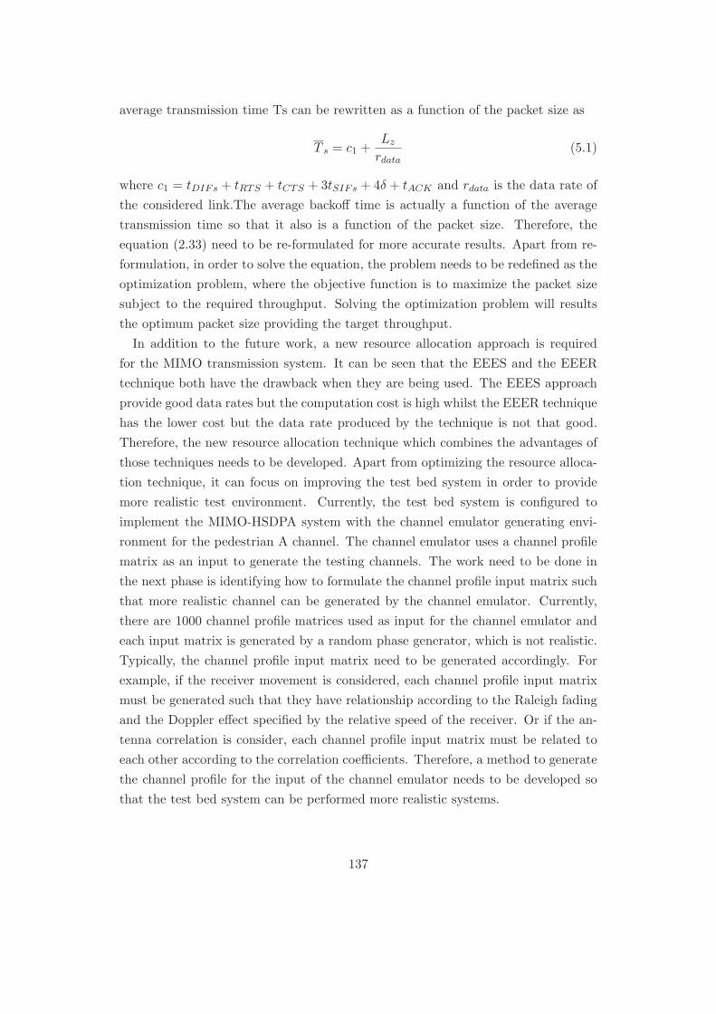
average transmission time Ts can be rewritten as a function of the packet size as

T s = c1 +Lz

rdata(5.1)

where c1 = tDIFs + tRTS + tCTS + 3tSIFs + 4δ + tACK and rdata is the data rate of

the considered link.The average backoff time is actually a function of the average

transmission time so that it also is a function of the packet size. Therefore, the

equation (2.33) need to be re-formulated for more accurate results. Apart from re-

formulation, in order to solve the equation, the problem needs to be redefined as the

optimization problem, where the objective function is to maximize the packet size

subject to the required throughput. Solving the optimization problem will results

the optimum packet size providing the target throughput.

In addition to the future work, a new resource allocation approach is required

for the MIMO transmission system. It can be seen that the EEES and the EEER

technique both have the drawback when they are being used. The EEES approach

provide good data rates but the computation cost is high whilst the EEER technique

has the lower cost but the data rate produced by the technique is not that good.

Therefore, the new resource allocation technique which combines the advantages of

those techniques needs to be developed. Apart from optimizing the resource alloca-

tion technique, it can focus on improving the test bed system in order to provide

more realistic test environment. Currently, the test bed system is configured to

implement the MIMO-HSDPA system with the channel emulator generating envi-

ronment for the pedestrian A channel. The channel emulator uses a channel profile

matrix as an input to generate the testing channels. The work need to be done in

the next phase is identifying how to formulate the channel profile input matrix such

that more realistic channel can be generated by the channel emulator. Currently,

there are 1000 channel profile matrices used as input for the channel emulator and

each input matrix is generated by a random phase generator, which is not realistic.

Typically, the channel profile input matrix need to be generated accordingly. For

example, if the receiver movement is considered, each channel profile input matrix

must be generated such that they have relationship according to the Raleigh fading

and the Doppler effect specified by the relative speed of the receiver. Or if the an-

tenna correlation is consider, each channel profile input matrix must be related to

each other according to the correlation coefficients. Therefore, a method to generate

the channel profile for the input of the channel emulator needs to be developed so

that the test bed system can be performed more realistic systems.

137

Moreover, for the future work, it can be seen that the pre-coding scheme using in

this thesis, the eigen vector pre-coding and the channel inverse pre-coding approach

cannot be used with the proposed resource allocation scheme. Thus, the new pre-

coding scheme is required to solve the correlated channel in the MIMO transmission

system. Last, it is worth to extend the work to LTE 4G systems. As the LTE

uses the new air interface and the resources are limited as the 3G HSDPA, the

LTE system also requires the resource allocation technique to optimize the system

performance.

138

Appendix 1

1.1 Introduction to LabVIEW the Graphical-Based

Programming

LabVIEW is graphical-based programming introduced by National Instrument. Lab-

VIEW creates programs by connecting graphical blocks, which represent functions,

together. A set of function blocks which is wired operates specified tasks designed

by a user. The programming in the LabVIEW is also known as dataflow program-

ming, which construct a program from nodes and lines. The lines have a function to

carry variables and data which are generated by the nodes. since the function blocks

can appear simultaneously in the same time line, LabVIEW can performs parallel

execution or multi-threading, which makes LabVIEW to be fast and a powerful

programming language.

Originally, LabVIEW is designed for data acquisition and monitoring but,now,

the function blocks of LabVIEW have been developed to cover many areas of re-

search, including signal processing and communication. The software produced by

LabVIEW consists of two parts, front panel Figure 1.1 and block diagram Figure 1.2.

The front panel contains all inputs and outputs of the program and it is used to

interface with the user. The block diagram is where the program is written. The

program is simply created by dragging and dropping the function blocks and con-

nects them together in the block diagram part. As LabVIEW is made for the

data acquisition systems, LabVIEW basically widely supports communication with

hardware devices and it is compatible with driver software produced many manu-

facturers. The graphical programming is very easy to program and to understand

so that users can spend only a short time to learn and create a usable software. As

study conducted in [107], the LabVIEW was employed to teach the elementary of

digital signal processing course for new students. The work evaluated the effective-

ness of LabVIEW when using in teaching. The results was compared to Matlab but

it is not clear that which one is better. However, it was suggested that LabVIEW

can make teaching much more simple, because the instructor easily identify the task

139

Figure 1.1: Front panel of LabVIEW

140

Figure 1.2: Block diagram of LabVIEW

141

given to the student on the graphical-based programming. In addition, LabVIEW

is designed to support running in real-time environments so that the response time

is exceptional faster than Matlab [108]. LabVIEW and Matlab are examined on

the non-linear curve fitting algorithm in [109]. It has been found that LabVIEW

is less accuracy in term of data precision than Matlab, but LabVIEW has a better

performance in term of execution time and hardware interface. It was suggested

that a Matlab script node in LabVIEW can be used in order to take full advantage

from both platforms. In this thesis, a LabVIEW is mainly exploited to make testing

software, since the software will be used in connection with FPGA-based hardware

in order to construct a test bed system for the MIMO-HSDPA technique.

1.2 Building the Test Bed System

Our objective is to build a test bed system for testing the proposed MIMO-HSDPA

techniques. To achieve the goal, we have spent time and constructed many versions

of the test bed system. We have found advantages and drawbacks of each test bed

system and, eventually, we decide to use the LabVIEW-PXIe systems, because it is

powerful and is able to provide the test environments we want. On developing the

LabVIEW-PXIe test bed system, we fully receive help from National Instrument

and we would like to acknowledge them for the good support. In this section, each

test bed system will be described.

1.2.1 The GNR radio-USRP Test Bed System

The first version of the test bed system is based on the GNU radio and the USRP

devices, which will be used to operate the time and frequency synchronization tech-

nique proposed in the last section. The GNU radio is an open-source software, which

is free to download and the USRP is low cost devices so that the system cost is not

expensive. But running the GNU radio is required experience in a Linux system

as it is based on Linux operating system and, moreover, the GNU radio does not

provide signal processing tool boxes which is required to operate the time and fre-

quency synchronization. The GNU radio is employed only for interfacing between

transceiver devices and a user and, to perform the signal processing, the system still

requires Matlab. Hence, operating signal transmission on the GNU radio-USRP test

bed need to switch between Matlab and the GNU radio in order to get the received

constellation, which is absolutely inconvenient.

142

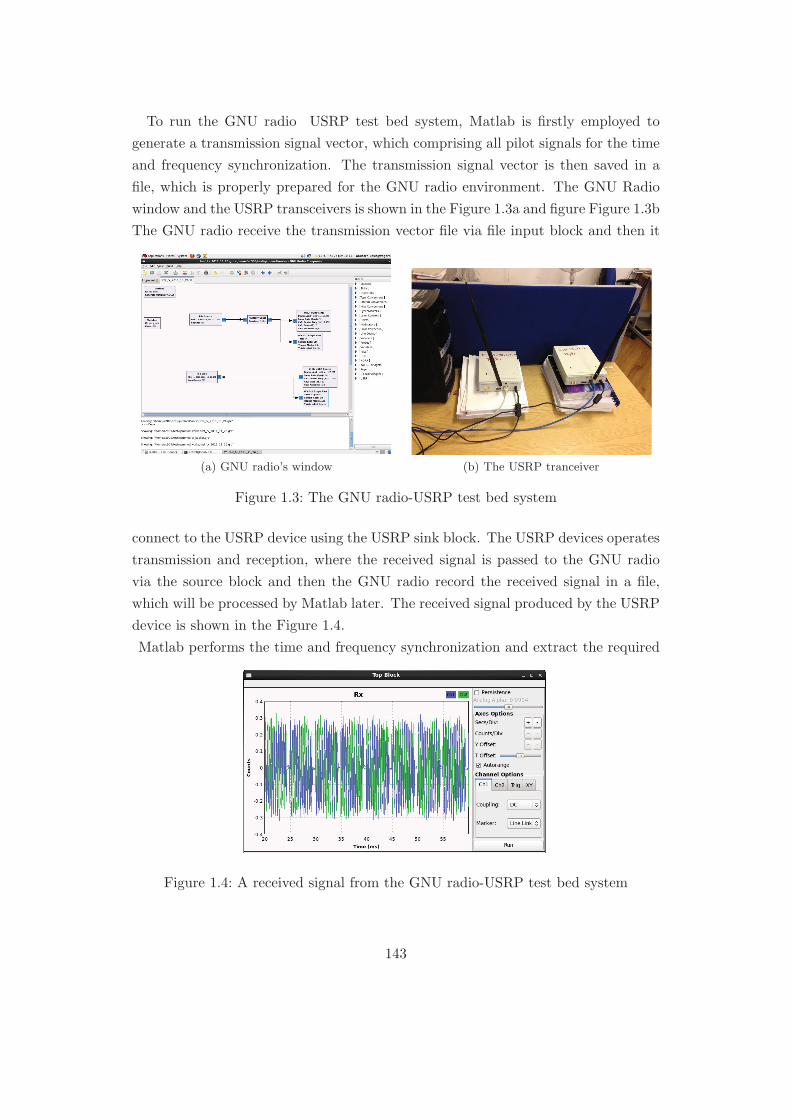
To run the GNU radio USRP test bed system, Matlab is firstly employed to

generate a transmission signal vector, which comprising all pilot signals for the time

and frequency synchronization. The transmission signal vector is then saved in a

file, which is properly prepared for the GNU radio environment. The GNU Radio

window and the USRP transceivers is shown in the Figure 1.3a and figure Figure 1.3b

The GNU radio receive the transmission vector file via file input block and then it

(a) GNU radio’s window

(b) The USRP tranceiver

Figure 1.3: The GNU radio-USRP test bed system

connect to the USRP device using the USRP sink block. The USRP devices operates

transmission and reception, where the received signal is passed to the GNU radio

via the source block and then the GNU radio record the received signal in a file,

which will be processed by Matlab later. The received signal produced by the USRP

device is shown in the Figure 1.4.

Matlab performs the time and frequency synchronization and extract the required

Figure 1.4: A received signal from the GNU radio-USRP test bed system

143

data from the received signal. After that, it run the signal processing on the data

packet to get the received constellation plot. The received signal data packet and the

received constellation plot of 4-QAM are given as in the Figure 1.5a and Figure 1.5b

As it can be seen, the received constellation is shifted as frequency offset correction

(a) GNU radio’s received packet (b) The received constellation

Figure 1.5: The GNU radio-USRP’s received signal

is not accurate, but it demonstrated that the time and frequency synchronization

can be employed for transmission and reception the signal on the test bed system.

Later, in Matlab 2011b, the Simulink tool boxes that used to connect to the USRP

device are available. Therefore, there is no need to use the GNU radio anymore.

1.2.2 The Matlab-USRP Test Bed System

The second version of the test bed system has been developed based-on the Matlab

USRP devices, which was conducted by [84]. In the work, the frequency offset prob-

lem was analyzed and the more precise frequency correction method was proposed

so that the QAM transceiver is enhanced. Using only Matlab simplifies the system,

since the signal processing and communication can be run in the same program. The

system is almost the same as the first version except the GNU radio part is replaced

by the Matlabs Simulink, which is employed to communicate with the USRP devices.

The Matlabs Simulink is shown in the Figure 1.6 The Simulink block receives a trans-

mission signal vector file and then passes the file to the communication block, which

interface with the transmission USRP device. At the receiver, the receive USRP de-

vice acquires the signal and deliver to the module which produce the received signal

vector file. Since the frequency offset problem is solved, the received constellation

144

Figure 1.6: Matlab’s simulink block for connecting to the USRP transceiver

diagram is received correctly, as shown by the Figure 1.7 However, Matlab is slow

(a) The constellation diagram of thetransmitted signal

(b) The constellation diagram of thereceived signal

Figure 1.7: The GNU radio-USRP’s received signal

in data processing as it is a text-based program, where source code needs to be

interpreted into machine language and execute in a sequence. Especially, when run-

ning the Simulink, the run time is significantly slow, because each Simulink block

need to be interpreted into Matlab code and to the machine language afterward.

Moreover, connection between the USRP devices and Matlab is not good. Matlab

spent long time to establish connection, which make program running slowly. Mat-

lab is powerful in computation but it is not suitable to be used in real time. Since

fast response time program is required for the test bed system, LabVIEW provided

145

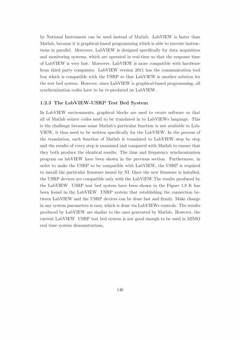
by National Instrument can be used instead of Matlab. LabVIEW is faster than

Matlab, because it is graphical-based programming which is able to execute instruc-

tions in parallel. Moreover, LabVIEW is designed specifically for data acquisition

and monitoring systems, which are operated in real-time so that the response time

of LabVIEW is very fast. Moreover, LabVIEW is more compatible with hardware

from third party companies. LabVIEW version 2011 has the communication tool

box which is compatible with the USRP so that LabVIEW is another solution for

the test bed system. However, since LabVIEW is graphical-based programming, all

synchronization codes have to be re-produced on LabVIEW.

1.2.3 The LabVIEW-USRP Test Bed System

In LabVIEW environments, graphical blocks are used to create software so that

all of Matlab source codes need to be translated in to LabVIEWs language. This

is the challenge because some Matlab’s particular function is not available in Lab-

VIEW, it thus need to be written specifically for the LabVIEW. In the process of

the translation, each function of Matlab is translated to LabVIEW step by step

and the results of every step is examined and compared with Matlab to ensure that

they both produce the identical results. The time and frequrency synchronization

program on labVIEW have been shown in the previous section. Furthermore, in

order to make the USRP to be compatible with LabVIEW, the USRP is required

to install the particular firmware issued by NI. Once the new firmware is installed,

the USRP devices are compatible only with the LabVIEW.The results produced by

the LabVIEW USRP test bed system have been shown in the Figure 1.8 It has

been found in the LabVIEW USRP system that establishing the connection be-

tween LabVIEW and the USRP devices can be done fast and firmly. Make change

in any system parameters is easy, which is done via LabVIEWs controls. The results

produced by LabVIEW are similar to the ones generated by Matlab. However, the

current LabVIEW USRP test bed system is not good enough to be used in MIMO

real time system demonstrations.

146

(a) 4-QAM transmission

(b) 16-QAM transmission

Figure 1.8: The LabVIEW - USRP QAM transmission

This is because firstly the current system can generate only noisy wireless channels.

To generate a multipath fading channel for the MIMO-HSDPA system, the distance

147

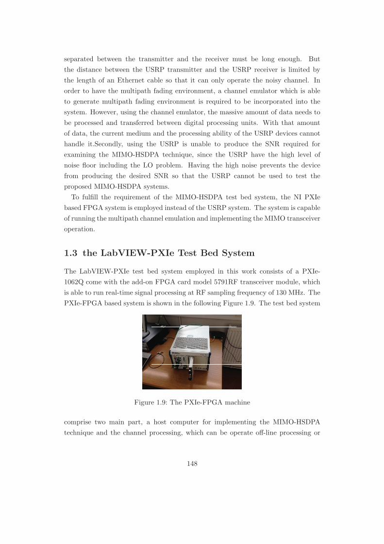
separated between the transmitter and the receiver must be long enough. But

the distance between the USRP transmitter and the USRP receiver is limited by

the length of an Ethernet cable so that it can only operate the noisy channel. In

order to have the multipath fading environment, a channel emulator which is able

to generate multipath fading environment is required to be incorporated into the

system. However, using the channel emulator, the massive amount of data needs to

be processed and transferred between digital processing units. With that amount

of data, the current medium and the processing ability of the USRP devices cannot

handle it.Secondly, using the USRP is unable to produce the SNR required for

examining the MIMO-HSDPA technique, since the USRP have the high level of

noise floor including the LO problem. Having the high noise prevents the device

from producing the desired SNR so that the USRP cannot be used to test the

proposed MIMO-HSDPA systems.

To fulfill the requirement of the MIMO-HSDPA test bed system, the NI PXIe

based FPGA system is employed instead of the USRP system. The system is capable

of running the multipath channel emulation and implementing the MIMO transceiver

operation.

1.3 the LabVIEW-PXIe Test Bed System

The LabVIEW-PXIe test bed system employed in this work consists of a PXIe-

1062Q come with the add-on FPGA card model 5791RF transceiver module, which

is able to run real-time signal processing at RF sampling frequency of 130 MHz. The

PXIe-FPGA based system is shown in the following Figure 1.9. The test bed system

Figure 1.9: The PXIe-FPGA machine

comprise two main part, a host computer for implementing the MIMO-HSDPA

technique and the channel processing, which can be operate off-line processing or

148

real-time FPGA based RF emulation. The channel also have been used in [110]

to test pre-coding schemes over MIMI-OFDM systems. The PXIe-FPGA based

system for the MIMO-HSDPA system can be demonstrated as the block diagram in

Figure 1.10

Figure 1.10: The Labview-PXIe block diagram

149

Figure 1.11: The LabVIEW-PXIe test bed’s front panel

i

References

[1] I. OReilly Media, “802.11ac : A survival guide,”

http://chimera.labs.oreilly.com/books/1234000001739/ch04.html, 2013.

[2] Invocom, “Rts/cts mechanism,” http://www.invocom.et.put.poznan.pl/∼invocom/C/P1-4/p1-4 en/p1-

2013.

[3] A. Toskala and H. Holma, WCDMA for UMTS: Radio Access for Third Gen-

eration Mobile Communications. Wiley, 2001.

[4] 3GPP, “Version 5 of technical specifications and

technical reports for a utran-based 3gpp system,”

http://www.3gpp.org/specifications-/Releases/article/release-5, 2003.

[5] C. Mehlfuhrer, S. Caban, and M. Rupp, “Cellular system physical layer

throughput: How far off are we from the shannon bound?” Wireless Commu-

nications, IEEE, vol. 18, no. 6, pp. 54–63, 2011.

[6] J. G. Andrews, W. Choi, and R. W. Heath Jr, “Mimo in 3g cellular systems:

Challenges and future directions,” submitted to IEEE Communications Mag-

azine, 2005.

[7] 3GPP, “3gpp release 99 - version 3 of technical specifica-

tions and technical reports for a utran-based 3gpp system,”

http://www.3gpp.org/specifications/Releases/article/release-1999, 1999.

[8] M. Cvitkovic, B. Modlic, and G. Sisul, “High speed downlink packet access

principles,” in ELMAR, 2007. IEEE, 2007, pp. 125–128.

[9] 3GPP, “Version 7 technical specifications and tech-

nical reports for a utran-based 3gpp system,”

http://www.3gpp.org/specifications-/Releases/article/release-7, 2007.

ii

[10] J. Sharony, “Introduction to wireless mimo–theory and applications,” CE-

WITCenter of Excellence in Wireless and Informational Technology, Stony

Brook University, IEEE LI, 2006.

[11] A. J. Paulraj, D. A. Gore, R. U. Nabar, and H. Bolcskei, “An overview of

mimo communications-a key to gigabit wireless,” Proceedings of the IEEE,

vol. 92, no. 2, pp. 198–218, 2004.

[12] B. Clerckx and C. Oestges, MIMO Wireless Networks: Channels, Techniques

and Standards for Multi-Antenna, Multi-User and Multi-Cell Systems, 2nd ed.

Academic Press, 2013.

[13] J. Winters, “Understanding mimo : Part i,”

http://www.eetimes.com/document.asp?doc id=1273367, 2005.

[14] E. Dahlman, S. Parkvall, J. Skold, and P. Beming, 3G evolution: HSPA and

LTE for mobile broadband. Access Online via Elsevier, 2010.

[15] A. J. Paulraj and T. Kailath, “Increasing capacity in wireless broadcast sys-

tems using distributed transmission/directional reception (dtdr),” Sep. 6 1994,

uS Patent 5,345,599.

[16] G. J. Foschini, “Layered space-time architecture for wireless communication in

a fading environment when using multi-element antennas,” Bell labs technical

journal, vol. 1, no. 2, pp. 41–59, 1996.

[17] P. W. Wolniansky, G. J. Foschini, G. Golden, and R. A. Valenzuela, “V-

blast: An architecture for realizing very high data rates over the rich-scattering

wireless channel,” in Signals, Systems, and Electronics, 1998. ISSSE 98. 1998

URSI International Symposium on. IEEE, 1998, pp. 295–300.

[18] www.Radio Electronics.com, “Ieee 802.11n standards,”

http://www.radio-electronics.com/info/wireless/wi-fi/ieee-802-11n.php,

2013.

[19] Novarlum, “Ieee 802.11n wireless lan ; opportunity and challenge,”

http://www.novarum.com/documents/802.11nWPv5.5.pdf, 2007.

[20] “802.11n primer,” http://airmagnet.flukenetworks.com/assets/whitepaper/WP-802.11nPrimer.pdf,

2008.

iii

[21] L. C. Godara, Handbook of antennas in wireless communications. CRC press,

2010, vol. 4.

[22] T.-H. Ha and D.-H. Tuan, “Characterizing mobile-radio propagation,”

http://cnx.org/content/m15528/latest/?collection=col10474/latest, 2013.

[23] P. Almers, E. Bonek, A. Burr, N. Czink, M. Debbah, V. Degli-Esposti, H. Hof-

stetter, P. Kyo, D. Laurenson, G. Matz et al., “Survey of channel and radio

propagation models for wireless mimo systems,” EURASIP Journal on Wire-

less Communications and Networking, vol. 2007, 2007.

[24] A. Forenza, D. J. Love, and R. W. Heath, “Simplified spatial correlation mod-

els for clustered mimo channels with different array configurations,” Vehicular

Technology, IEEE Transactions on, vol. 56, no. 4, pp. 1924–1934, 2007.

[25] J. P. Kermoal, L. Schumacher, K. I. Pedersen, P. E. Mogensen, and F. Fred-

eriksen, “A stochastic mimo radio channel model with experimental valida-

tion,” Selected Areas in Communications, IEEE Journal on, vol. 20, no. 6, pp.

1211–1226, 2002.

[26] A. Colvin, “Csma with collision avoidance,” Computer Communications,

vol. 6, no. 5, pp. 227–235, 1983.

[27] J. Zhou, “Resource allocation in ad hoc networks,” PhD Thesis, Imperial

College London, April 2011.

[28] X. Wang, J. Garcia-Luna-Aceves, and H. R. Sadjadpour, “Performance model-

ing of mac and multipath routing interactions in multi-hop wireless networks.”

[29] C. Hu, H. Kim, and J. C. Hou, “An analysis of the binary exponential backoff

algorithm in distributed mac protocols,” Citeseer, Tech. Rep., 2005.

[30] M. M. Carvalho and J. J. Garcia-Luna-Aceves, “A scalable model for channel

access protocols in multihop ad hoc networks,” in Proceedings of the 10th

annual international conference on Mobile computing and networking. ACM,

2004, pp. 330–344.

[31] J. Zhou and M. Gurcan, “An improved multicode cdma transmission method

for ad hoc networks,” in Wireless Communications and Networking Confer-

ence, 2009. WCNC 2009. IEEE. IEEE, 2009, pp. 1–6.

iv

[32] N. Simulator, “ns-2.35,” http://www.isi.edu/nsnam/ns/, 2011.

[33] D. B. Green and A. Obaidat, “An accurate line of sight propagation perfor-

mance model for ad-hoc 802.11 wireless lan (wlan) devices,” in Communica-

tions, 2002. ICC 2002. IEEE International Conference on, vol. 5. IEEE,

2002, pp. 3424–3428.

[34] J. Deng, B. Liang, and P. K. Varshney, “Tuning the carrier sensing range of

ieee 802.11 mac,” in Global Telecommunications Conference, 2004. GLOBE-

COM’04. IEEE, vol. 5. IEEE, 2004, pp. 2987–2991.

[35] T. S. Rappaport et al., Wireless communications: principles and practice.

Prentice Hall PTR New Jersey, 1996, vol. 2.

[36] R. Gallager, “Low-density parity-check codes,” Information Theory, IRE

Transactions on, vol. 8, no. 1, pp. 21–28, 1962.

[37] C. Berrou, A. Glavieux, and P. Thitimajshima, “Near shannon limit error-

correcting coding and decoding: Turbo-codes. 1,” in Communications, 1993.

ICC 93. Geneva. Technical Program, Conference Record, IEEE International

Conference on, vol. 2. IEEE, 1993, pp. 1064–1070.

[38] 3GPP, “Third generation partnership project technical spec-

ification group radio access network working group 1, ”

multiplexing and channel coding (fdd),” ts 25.212 v2.0.1,”

http://www.3gpp.org/ftp/tsg ran/wg1 rl1/TSGR1 07/Docs/Pdfs/R1-99a86.pdf,

1999.

[39] G. D. Forney Jr and G. Ungerboeck, “Modulation and coding for linear gaus-

sian channels,” Information Theory, IEEE Transactions on, vol. 44, no. 6, pp.

2384–2415, 1998.

[40] I. Chih-Lin and R. D. Gitlin, “Multi-code cdma wireless personal commu-

nications networks,” in Communications, 1995. ICC’95 Seattle,’Gateway to

Globalization’, 1995 IEEE International Conference on, vol. 2. IEEE, 1995,

pp. 1060–1064.

[41] H. Holma, A. Toskala et al., Wcdma for Umts. Citeseer, 2000, vol. 4.

v

[42] S. Mueller, R. P. Tsang, and D. Ghosal, “Multipath routing in mobile ad hoc

networks: Issues and challenges,” in Performance Tools and Applications to

Networked Systems. Springer, 2004, pp. 209–234.

[43] A. Tsirigos and Z. J. Haas, “Analysis of multipath routing-part i: The effect

on the packet delivery ratio,” Wireless Communications, IEEE Transactions

on, vol. 3, no. 1, pp. 138–146, 2004.

[44] N. Jain, D. K. Madathil, and D. P. Agrawal, “Energy aware multi-path routing

for uniform resource utilization in sensor networks,” in Information Processing

in Sensor Networks. Springer, 2003, pp. 473–487.

[45] D. Kim, W. Lee, B.-N. Park, J. Kim, C. Shin, and C. Shin, “A power bal-

anced multipath routing protocol inwireless ad-hoc sensor networks,” in Com-

puter and Information Technology, 2006. CIT’06. The Sixth IEEE Interna-

tional Conference on. IEEE, 2006, pp. 222–222.

[46] P. Sambasivam, A. Murthy, and E. M. Belding-Royer, “Dynamically adaptive

multipath routing based on aodv,” in Proc. 3rd Annual Mediterranean Ad Hoc

Networking Workshop, 2004.

[47] F. Baccelli, B. B laszczyszyn, and P. Muhlethaler, “Time–space opportunistic

routing in wireless ad hoc networks: algorithms and performance optimization

by stochastic geometry,” The Computer Journal, vol. 53, no. 5, pp. 592–609,

2010.

[48] S.-J. Lee and M. Gerla, “Aodv-br: Backup routing in ad hoc networks,”

in Wireless Communications and Networking Confernce, 2000. WCNC. 2000

IEEE, vol. 3. IEEE, 2000, pp. 1311–1316.

[49] M. K. Gurcan, H. Ab Ghani, J. Zhou, and A. Chungtragarn, “Bit energy

consumption minimization for multi-path routing in ad hoc networks,” The

Computer Journal, vol. 54, no. 6, pp. 944–959, 2011.

[50] A. Pandi, “Hop trellis modelling in ad hoc networks,” MSc Dissertation, Im-

perial College London, Sep 2009.

[51] A. Destounis, “On hsdpa femtocell technology for ad hoc and wireless sensor

networks: investigation of the routing problem.” MSc Dissertation, Imperial

College London, Sep 2010.

vi

[52] T. H. Cormen, C. E. Leiserson, R. L. Rivest et al., “Dijkstra\’s algorithm,”

2001.

[53] M. K. Gurcan, I. Ma, A. Chungtragarn, and H. Joudeh, “System value-based

optimum spreading sequence selection for high-speed downlink packet access

(hsdpa) mimo,” EURASIP J. Wireless Comm. and Networking, pp. 74–74,

2013.

[54] J. Cioffi, “Class reader for ee379a–digital communication: Signal processing,”

http://www.stanford.edu/class/ee379a, 2003.

[55] T.-J. Ho and B.-S. Chen, “Robust minimax mse equalizer designs for mimo

wireless communications with time-varying channel uncertainties,” Signal Pro-

cessing, IEEE Transactions on, vol. 58, no. 11, pp. 5835–5844, 2010.

[56] J.-B. Landre, A. Saadani, and F. Ortolan, “Hsdpa radio capacity improve-

ment with advanced devices,” in Vehicular Technology Conference (VTC 2010-

Spring), 2010 IEEE 71st, 2010, pp. 1–5.

[57] T. Nihtila and V. Haikola, “Hsdpa performance with dual stream mimo in

a combined macro-femto cell network,” in Vehicular Technology Conference

(VTC 2010-Spring), 2010 IEEE 71st, 2010, pp. 1–5.

[58] M. Gurcan, I. Ma, and H. Ab Ghani, “The interference-reduced energy loading

for multi-code hsdpa systems,” EURASIP Journal on Wireless Communica-

tions and Networking, vol. 2012, no. 1, pp. 1–17, 2012.

[59] W. Jian, Y. Longxiang, and L. Xu, “Resource allocation based on linear water-

filling algorithm in cr systems,” in Wireless Communications, Networking and

Mobile Computing (WiCOM), 2011 7th International Conference on, 2011,

pp. 1–4.

[60] J. Xu, L. Qiu, and S. Zhang, “Energy efficient iterative waterfilling for the

mimo broadcasting channels,” in Wireless Communications and Networking

Conference (WCNC), 2012 IEEE, 2012, pp. 198–203.

[61] V. Subramanian, R. Berry, and R. Agrawal, “Joint scheduling and resource

allocation in cdma systems,” Information Theory, IEEE Transactions on,

vol. 56, no. 5, pp. 2416–2432, 2010.

vii

[62] N. Papandreou and T. Antonakopoulos, “Bit and power allocation in con-

strained multicarrier systems: the single-user case,” EURASIP Journal on

Advances in Signal Processing, vol. 2008, p. 11, 2008.

[63] P. Layec, R. Visoz, and A. Berthet, “Sum discrete-rate maximization with

rate and power control in layered space-time coding,” Communications, IEEE

Transactions on, vol. 57, no. 3, pp. 789–800, 2009.

[64] J. Mitola, “The software radio architecture,” Communications Magazine,

IEEE, vol. 33, no. 5, pp. 26–38, 1995.

[65] SDR, “What is software defined radio,”

http://www.wirelessinnova-tion.org/assets/documents/SoftwareDefinedRadio.pdf,

2013.

[66] M. Dardaillon, K. Marquet, T. Risset, and A. Scherrer, “Software defined

radio architecture survey for cognitive testbeds,” in Wireless Communications

and Mobile Computing Conference (IWCMC), 2012 8th International. IEEE,

2012, pp. 189–194.

[67] A. A. Tabassam, F. A. Ali, S. Kalsait, and M. U. Suleman, “Building software-

defined radios in matlab simulink-a step towards cognitive radios,” in Com-

puter Modelling and Simulation (UKSim), 2011 UKSim 13th International

Conference on. IEEE, 2011, pp. 492–497.

[68] M. Dusek, V. Derbek, A. Povalac, J. Sebesta, and R. Marsalek, “Hardware

and software stack for an sdr-based rfid test platform,” in RFID Technol-

ogy (EURASIP RFID), 2012 Fourth International EURASIP Workshop on.

IEEE, 2012, pp. 41–45.

[69] D. Bates, S. Henriksen, B. Ninness, and S. R. Weller, “A 4× 4 fpga-based

wireless testbed for lte applications,” in Personal, Indoor and Mobile Radio

Communications, 2008. PIMRC 2008. IEEE 19th International Symposium

on. IEEE, 2008, pp. 1–5.

[70] C. Mehlfuhrer, S. Caban, and M. Rupp, “Measurement-based performance

evaluation of mimo hsdpa,” Vehicular Technology, IEEE Transactions on,

vol. 59, no. 9, pp. 4354–4367, 2010.

[71] M. ETTUS, “Universal software radio peripheral (usrp),”

http://www.ettus.com/, 2013.

viii

[72] M. Rupp, C. Mehlfuhrer, S. Caban, R. Langwieser, L. W. Mayer, and

A. L. Scholtz, “Testbeds and rapid prototyping in wireless system design,”

EURASIP Newsletter, vol. 17, no. 3, pp. 32–50, 2006.

[73] S. Caban, C. Mehlfu, R. Langwieser, A. L. Scholtz, M. Rupp et al., “Vienna

mimo testbed,” EURASIP Journal on Advances in Signal Processing, vol.

2006, 2006.

[74] E. Blossom, “Gnu radio: tools for exploring the radio frequency spectrum,”

Linux journal, vol. 2004, no. 122, p. 4, 2004.

[75] N. Shahin, N. J. LaSorte, S. A. Rajab, and H. H. Refai, “802.11 g channel

characterization utilizing labview and ni-usrp,” in Instrumentation and Mea-

surement Technology Conference (I2MTC), 2013 IEEE International. IEEE,

2013, pp. 753–756.

[76] H. Castro and J. A. Taborda, “Rapid prototyping of chaotic generators using

labview-fpga,” in Circuits and Systems (CWCAS), 2012 IEEE 4th Colombian

Workshop on. IEEE, 2012, pp. 1–6.

[77] M. Rupp, S. Caban, and C. Mehlfuhrer, “Challenges in building mimo

testbeds,” in Proc. 15th European Signal Processing Conference (EUSIPCO

2007), Poznan, Poland, 2007.

[78] J. A. Garcıa-Naya, M. Gonzalez-Lopez, and L. Castedo, “An overview of mimo

testbed technology,” in Proceedings of the 4th International Symposium on Im-

age and Video Communications over Fixed and Mobile Networks (ISIVC’08),

2008.

[79] R. Jain, “Channel models a tutorial1,” 2007.

[80] ITU.R.M.1225, “Guidelines for evaluation of radio transmission technologies

for imt-2000,” 1997.

[81] E. Vinko, S. Laurentm, K. Persefoni, M. Andreas, B. S. Daniel, G. Y. Alexei,

and et al, “Tgn channel models,” 2004.

[82] N. I. Corporate, “Labview,” http://www.ni.com/labview/, 2013.

[83] I. The Math Works, “Matlab,” http://www.mathworks.co.uk-/products/matlab/,

2013.

ix

[84] H. Joudeh, “Qam transmission using usrp and matlab,” MSc Dissertation,

Imperial College London, May 2012.

[85] S. Boumard and A. Mammela, “Robust and accurate frequency and timing

synchronization using chirp signals,” Broadcasting, IEEE Transactions on,

vol. 55, no. 1, pp. 115–123, 2009.

[86] L. M. DAO, “Wireless communications using chirp signals,” MSc Dissertation,

Waseda University, Jun 2008.

[87] H. Bolcskei, “Blind estimation of symbol timing and carrier frequency offset

in wireless ofdm systems,” Communications, IEEE Transactions on, vol. 49,

no. 6, pp. 988–999, 2001.

[88] D.-S. Shiu, G. J. Foschini, M. J. Gans, and J. M. Kahn, “Fading correlation and

its effect on the capacity of multielement antenna systems,” Communications,

IEEE Transactions on, vol. 48, no. 3, pp. 502–513, 2000.

[89] A. M. Tulino, A. Lozano, and S. Verdu, “Impact of antenna correlation on the

capacity of multiantenna channels,” Information Theory, IEEE Transactions

on, vol. 51, no. 7, pp. 2491–2509, 2005.

[90] A. G. Burr, “Capacity bounds and estimates for the finite scatterers mimo

wireless channel,” Selected Areas in Communications, IEEE Journal on,

vol. 21, no. 5, pp. 812–818, 2003.

[91] ——, “Multiplexing gain of multiuser mimo on finite scattering channels,” in

Wireless Communication Systems (ISWCS), 2010 7th International Sympo-

sium on. IEEE, 2010, pp. 466–470.

[92] M. Debbah and R. R. Muller, “Mimo channel modeling and the principle of

maximum entropy,” Information Theory, IEEE Transactions on, vol. 51, no. 5,

pp. 1667–1690, 2005.

[93] L. Wood and W. S. Hodgkiss, “Understanding the weichselberger model: A

detailed investigation,” in Military Communications Conference, 2008. MIL-

COM 2008. IEEE. IEEE, 2008, pp. 1–7.

[94] C. Oestges, “Validity of the kronecker model for mimo correlated channels,” in

Vehicular Technology Conference, 2006. VTC 2006-Spring. IEEE 63rd, vol. 6.

IEEE, 2006, pp. 2818–2822.

x

[95] O. Fernandez, M. Domingo, and R. P. Torres, “Outdoor to indoor 2x2 wide-

band mimo channel modelling,” in Vehicular Technology Conference, 2009.

VTC Spring 2009. IEEE 69th. IEEE, 2009, pp. 1–5.

[96] A. A. Saleh and R. Valenzuela, “A statistical model for indoor multipath

propagation,” Selected Areas in Communications, IEEE Journal on, vol. 5,

no. 2, pp. 128–137, 1987.

[97] B. Holter, “On the capacity of the mimo channel: A tutorial introduction,” in

Proc. IEEE Norwegian Symposium on Signal Processing, 2001, pp. 167–172.

[98] A. Goldsmith, S. A. Jafar, N. Jindal, and S. Vishwanath, “Capacity limits of

mimo channels,” Selected Areas in Communications, IEEE Journal on, vol. 21,

no. 5, pp. 684–702, 2003.

[99] H. Bolcskei, D. Gesbert, and A. J. Paulraj, “On the capacity of ofdm-

based spatial multiplexing systems,” Communications, IEEE Transactions on,

vol. 50, no. 2, pp. 225–234, 2002.

[100] P. Scholar, “Literature survey for minimum euclidean distance based precoder

for mimo systems,” International Journal of Engineering, vol. 2, no. 1, 2013.

[101] M. Vu and A. Paulraj, “Mimo wireless linear precoding,” Signal Processing

Magazine, IEEE, vol. 24, no. 5, pp. 86–105, 2007.

[102] G. Lebrun, J. Gao, and M. Faulkner, “Mimo transmission over a time-varying

channel using svd,” Wireless Communications, IEEE Transactions on, vol. 4,

no. 2, pp. 757–764, 2005.

[103] W. Xu, X. Dong, and W.-S. Lu, “Mimo relaying broadcast channels with

linear precoding and quantized channel state information feedback,” Signal

Processing, IEEE Transactions on, vol. 58, no. 10, pp. 5233–5245, 2010.

[104] D. Gesbert, M. Kountouris, R. W. Heath, C.-B. Chae, and T. Salzer, “Shifting

the mimo paradigm,” Signal Processing Magazine, IEEE, vol. 24, no. 5, pp.

36–46, 2007.

[105] A. Wiesel, Y. C. Eldar, and S. Shamai, “Zero-forcing precoding and generalized

inverses,” Signal Processing, IEEE Transactions on, vol. 56, no. 9, pp. 4409–

4418, 2008.

xi

[106] F. Kaltenberger, D. Gesbert, R. Knopp, and M. Kountouris, “Correlation

and capacity of measured multi-user mimo channels,” in Personal, Indoor and

Mobile Radio Communications, 2008. PIMRC 2008. IEEE 19th International

Symposium on. IEEE, 2008, pp. 1–5.

[107] M. A. Yoder and B. A. Black, “Teaching dsp first with labview,” in Digital

Signal Processing Workshop, 12th-Signal Processing Education Workshop, 4th.

IEEE, 2006, pp. 278–280.

[108] W. Winiecki and P. Bilski, “Time aspects of virtual instrument designing,” in

Instrumentation and Measurement Technology Conference, 2003. IMTC’03.

Proceedings of the 20th IEEE, vol. 2. IEEE, 2003, pp. 913–918.

[109] H. Wen, J. Ma, M. Zhang, and G. Ma, “The comparison research of nonlinear

curve fitting in matlab and labview,” in Electrical & Electronics Engineering

(EEESYM), 2012 IEEE Symposium on. IEEE, 2012, pp. 74–77.

[110] Q. Liu, “Early state assessment report,” Formal report, Imperial College Lon-

don, July 2013.

xii