Mind Mappings: Enabling Efficient Algorithm-Accelerator

Mind Mappings: Enabling Efficient Algorithm-AcceleratorMapping Space Search

Kartik HegdeUniversity of Illinois atUrbana-Champaign, [email protected]

Po-An TsaiNVIDIA, USA

[email protected]

Sitao HuangUniversity of Illinois atUrbana-Champaign, [email protected]

Vikas ChandraFacebook, USA

[email protected]

Angshuman ParasharNVIDIA, USA

[email protected]

Christopher W. FletcherUniversity of Illinois atUrbana-Champaign, [email protected]

ABSTRACTModern day computing increasingly relies on specialization to sa-tiate growing performance and efficiency requirements. A corechallenge in designing such specialized hardware architecturesis how to perform mapping space search, i.e., search for an opti-mal mapping from algorithm to hardware. Prior work shows thatchoosing an inefficient mapping can lead to multiplicative-factorefficiency overheads. Additionally, the search space is not only largebut also non-convex and non-smooth, precluding advanced searchtechniques. As a result, previous works are forced to implementmapping space search using expert choices or sub-optimal searchheuristics.

This work proposes Mind Mappings, a novel gradient-basedsearch method for algorithm-accelerator mapping space search.The key idea is to derive a smooth, differentiable approximationto the otherwise non-smooth, non-convex search space. With asmooth, differentiable approximation, we can leverage efficientgradient-based search algorithms to find high-quality mappings.We extensively compare Mind Mappings to black-box optimiza-tion schemes used in prior work. When tasked to find mappingsfor two important workloads (CNN and MTTKRP), the proposedsearch finds mappings that achieve an average 1.40×, 1.76×, and1.29× (when run for a fixed number of steps) and 3.16×, 4.19×, and2.90× (when run for a fixed amount of time) better energy-delayproduct (EDP) relative to Simulated Annealing, Genetic Algorithmsand Reinforcement Learning, respectively. Meanwhile, Mind Map-pings returns mappings with only 5.32× higher EDP than a possiblyunachievable theoretical lower-bound, indicating proximity to theglobal optima.

CCS CONCEPTS• Computer systems organization→ Special purpose systems; •Software and its engineering→ Compilers.Permission to make digital or hard copies of all or part of this work for personal orclassroom use is granted without fee provided that copies are not made or distributedfor profit or commercial advantage and that copies bear this notice and the full citationon the first page. Copyrights for components of this work owned by others than ACMmust be honored. Abstracting with credit is permitted. To copy otherwise, or republish,to post on servers or to redistribute to lists, requires prior specific permission and/or afee. Request permissions from [email protected] ’21, April 19–23, 2021, Virtual, USA© 2021 Association for Computing Machinery.ACM ISBN 978-1-4503-8317-2/21/04. . . $15.00https://doi.org/10.1145/3445814.3446762

KEYWORDSprogrammable domain-specific accelerators, mapping space search,gradient-based search

ACM Reference Format:Kartik Hegde, Po-An Tsai, Sitao Huang, Vikas Chandra, AngshumanParashar, and Christopher W. Fletcher. 2021. Mind Mappings: EnablingEfficient Algorithm-Accelerator Mapping Space Search. In Proceedings of the26th ACM International Conference on Architectural Support for ProgrammingLanguages and Operating Systems (ASPLOS ’21), April 19–23, 2021, Virtual,USA. ACM, New York, NY, USA, 16 pages. https://doi.org/10.1145/3445814.3446762

1 INTRODUCTIONThe compound effect of the slowing of Moore’s law coupledwith a growing demand for efficient compute has ushered in anera of specialized hardware architectures. Due to their inherentperformance, energy, and area characteristics, these acceleratorsare driving innovation in diverse areas such as machine learn-ing [4, 20, 32, 38, 43, 69], medicine [22, 23, 41], cryptography [27, 61],etc. They are seeing a wide variety of deployments ranging fromcloud to edge—forcing designers to make complex design decisionsto achieve their efficiency objectives.

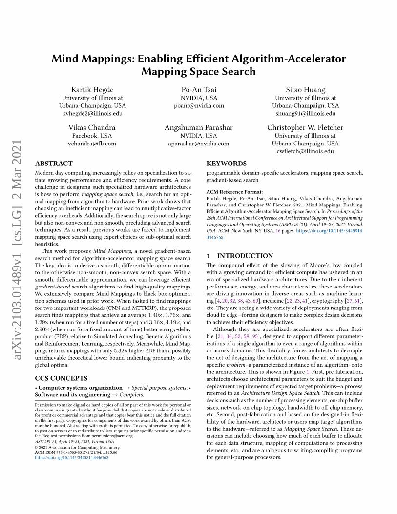
Although they are specialized, accelerators are often flexi-ble [21, 36, 52, 59, 95], designed to support different parameter-izations of a single algorithm to even a range of algorithms withinor across domains. This flexibility forces architects to decouplethe act of designing the architecture from the act of mapping aspecific problem–a parameterized instance of an algorithm–ontothe architecture. This is shown in Figure 1. First, pre-fabrication,architects choose architectural parameters to suit the budget anddeployment requirements of expected target problems—a processreferred to as Architecture Design Space Search. This can includedecisions such as the number of processing elements, on-chip buffersizes, network-on-chip topology, bandwidth to off-chip memory,etc. Second, post-fabrication and based on the designed-in flexi-bility of the hardware, architects or users map target algorithmsto the hardware—referred to as Mapping Space Search. These de-cisions can include choosing how much of each buffer to allocatefor each data structure, mapping of computations to processingelements, etc., and are analogous to writing/compiling programsfor general-purpose processors.

arX

iv:2

103.

0148

9v1

[cs

.LG

] 2

Mar

202

1

https://doi.org/10.1145/3445814.3446762

https://doi.org/10.1145/3445814.3446762

https://doi.org/10.1145/3445814.3446762

ASPLOS ’21, April 19–23, 2021, Virtual, USA Kartik Hegde, Po-An Tsai, Sitao Huang, Vikas Chandra, Angshuman Parashar, and Christopher W. Fletcher

Tile SizeLoopOrdering

Buffer Allocation

Mapping Space Search(This Work)

Tensor

Parallelism

PE PE PE

NoCBuffers

Accelerator Cost Model

AcceleratorRuntime Instance

AlgorithmSpecs

BufferBufferBufferBuffer

PE

Architecture Design Space Search

PEPE

NoC

PE

Budget

Architecture

Mapping

Figure 1: Architecture design and algorithm mapping inhardware accelerators.

Mapping space search is an important problem, and currentlyfaces severe scalability and performance challenges. To start, priorwork has shown that problem efficiency is very sensitive to thechoice of mapping [20, 36, 52, 59, 68, 69, 95]. Further, the same stud-ies illustrate how optimal mapping varies significantly dependingon problem size and parameters (e.g., DNN model parameters), re-source availability, performance and power requirements, etc. Thissuggests that mapping space search will constitute an increasingrecurring cost, as accelerators are re-targeted for new problems.

Making matters worse, simply gaining intuition for how tosearch through the map space, or how to pose the search to an au-tomated tool, is an ad-hoc and expert-driven process. Acceleratorslack consistent hardware-software abstractions, such as instructionset architectures (ISAs) in the general-purpose computing world,and instead rely on bespoke configurable hardware components de-signed to provide higher degrees of control and efficiency. Further,different accelerators tend to have different degrees of configurabil-ity in different hardware components, ranging from programmablenetworks on chip [52], buffers [36, 73], address generators [100],etc. While this may be suitable for experts with deep knowledgeof both the architecture and algorithm, it clearly does not scale tonon-experts programming new hardware with new algorithms.

Making matters even worse, while prior work has proposedtools and algorithms (i.e., Mappers) for automatically searching themap space, all existing approaches have serious limitations dueto search space complexity [3, 15, 36, 68, 102]. First, the searchspace is often high dimensional (i.e., each degree of configurabilityinduces a dimension), causing a combinatorial explosion of possiblemappings and rendering exhaustive techniques ineffective [68].Second, the search space is both non-convex (many local minima)and non-smooth (not differentiable), forcing prior work to rely onblack-box optimization [30] approaches.

To summarize, while configurable accelerators have demon-strated their potential, the lack of an efficient and high-qualityMapper hinders broader adoption.

1.1 This WorkThis paper addresses the challenges above by proposingMind Map-pings, a scalable and automated method to quickly and effectivelyperform mapping space search.

As mentioned previously, the key challenge hindering prior workis that mapping search space is non-smooth, forcing prior work toresort to black-box optimization techniques. This is because theaccelerator cost function—which search algorithms use to evaluatethe cost of a given candidate mapping—is non-smooth. For exam-ple, the cost function might be an architectural simulator or theaccelerator itself.

Mind Mappings addresses this challenge by constructing a dif-ferentiable approximation of the cost function, called the surro-gate [6, 75, 91]. Using the surrogate, Mind Mappings derives gradi-ents for the cost function, with respect to candidate mappings, anduses those gradients to perform a powerful first-order optimiza-tion technique, Gradient Descent [53, 54], to quickly find low-costmappings.

The key insight here is that the differentiable surrogate of theactual non-differentiable cost function can provide us with approx-imate gradients, which are sufficient to guide the search along thedirection of steepest descent, even in the absence of true gradients.This insight simultaneously improves map space search quality andreduces map space search time, as gradients by definition point inthe direction of the greatest reduction in cost.

Crucially, Mind Mappings formulates both predicting the cost ofa mapping and finding the optimal mapping as learning problems,thereby doing away with requiring expert knowledge in the targetdomain.

This paper makes the following contributions:(1) To the best of our knowledge, our work is the first to enable

target domain-independent mapping space search for pro-grammable accelerators. We require neither expert knowl-edge in the target application domain(s), nor any domainspecific heuristics for handling programmable hardware at-tributes.

(2) To the best of our knowledge, our work is the first to for-mulate mapping space search as a first-order optimizationproblem, enabling an efficient gradient-based search that isable to quickly find high-quality mappings.

(3) We extensively evaluate Mind Mappings across two targetalgorithms—CNNs and MTTKRP—comparing against multi-ple baseline search heuristics including simulated annealing(SA), genetic algorithms (GA), and reinforcement learning(RL). For CNNs and MTTKRP, the proposed search methodfinds mappings with an average 1.40×, 1.76×, and 1.29×(when run for a fixed number of steps) and 3.16×, 4.19×,and 2.90× (when run for a fixed amount of time) betterenergy-delay product over SA, GA, and RL, respectively.

(4) To facilitate further adoption, we provide a reference im-plementation of the Mind Mappings framework here: https://github.com/kartik-hegde/mindmappings.

2 BACKGROUNDIn this section, we formally define the algorithm-accelerator map-ping space search problem and elaborate with an example.

https://github.com/kartik-hegde/mindmappings

https://github.com/kartik-hegde/mindmappings

Mind Mappings: Enabling Efficient Algorithm-Accelerator Mapping Space Search ASPLOS ’21, April 19–23, 2021, Virtual, USA

2.1 Algorithm-Accelerator Mapping SpaceIn this paper, we assume that a hardware accelerator 𝑎 and a targetproblem 𝑝 is given, where a problem is a parameterized instanceof an algorithm. For example, if matrix multiplication is the targetalgorithm, an example target problem is a matrix multiplicationbetween two matrices of fixed shape (dimensions), irrespective ofthe contents of the matrices. We begin by defining a mapping𝑚and the mapping space𝑀 .

Definition 2.1. Mapping. A mapping𝑚 ∈ 𝑃0 × · · · × 𝑃𝐷−1 is a𝐷-tuple, where 𝐷 is the number of programmable attributes ofthe given accelerator 𝑎. Each element in the mapping vector,𝑚𝑑for 𝑑 ∈ [0, 𝐷) belongs to the domain of the 𝑑-th programmableattribute, 𝑃𝑑 .

Definition 2.2. Mapping Space.Given an accelerator 𝑎 and a targetproblem 𝑝 , we define a mapping space as

𝑀𝑎,𝑝 = {𝑚 ∈ 𝑃0 × · · · × 𝑃𝐷−1 | 𝑎(𝑚, 𝑖) == 𝑝 (𝑖) ∀𝑖 ∈ 𝐼𝑝 }

where 𝐼𝑝 denotes the possible inputs (e.g., all possible matrices witha specific shape) to a problem 𝑝 , 𝑎(𝑚, 𝑖) denotes the accelerator’soutput given mapping𝑚 and input 𝑖 , and 𝑝 (𝑖) denotes the goldenreference output given input 𝑖 for problem 𝑝 .

In other words,𝑀𝑎,𝑝 is the set of mappings that result in func-tional correctness for the given problem 𝑝 on the accelerator 𝑎.We call such mappings valid for 𝑎 and 𝑝 and write 𝑀𝑎,𝑝 as 𝑀 forshort when the context is clear. Intuitively, the different𝑚 ∈ 𝑀 canbe thought of as different “programs” representing problem 𝑝 onaccelerator 𝑎. An example of a mapping space is given in Section 3.

With this in mind, the size of the mapping space varies based onthe programmability of the underlying accelerator and the problem𝑝 . On one extreme, the size of𝑀 (denoted |𝑀 |) can be 1 for a fixed-function ASIC designed to execute one fixed problem. In general,|𝑀 | = 𝑂 (∏𝑑∈[0,𝐷) |𝑃𝑑 |), where the number of attributes 𝐷 andthe size of each attribute space |𝑃𝑑 | is large. The Big-Oh captureshow some mappings in the Cartesian product of assignments toprogrammable attributes may be invalid.

2.2 Mapping Space SearchMapping Space Search is the combinatorial search problem to findthe mapping𝑚𝑜𝑝𝑡 ∈ 𝑀 that minimizes the cost 𝑓 , where the costfunction 𝑓 is the optimization objective set by the designer (dis-cussed further in Section 2.3). That is,

𝑚𝑜𝑝𝑡 = argmin𝑚∈𝑀𝑎,𝑝

𝑓 (𝑎,𝑚) (1)

where the user specifies the problem 𝑝 and architecture 𝑎. Wedenote 𝑓 (𝑎,𝑚) as 𝑓 (𝑚) for short. In theory, mapping space searchcan be performed at compile time or at run time. In practice,programmable accelerators today either perform the search com-pletely offline, e.g., when compiling a new problem to the architec-ture [36, 51, 80], or partly offline/partly online [66].

In this paper, we assume 𝑓 is a function of 𝑎 and 𝑝—not theproblem input 𝑖 . This holds for several important workloads, e.g.,kernels in dense tensor algebra such as dense matrix multiplicationand deep neural network training/inference [68]. However, it doesnot hold when input-dependent optimizations, e.g., data sparsity,

influence cost [37]. We consider efficient mapping space search forinput-dependent mappings to be important future work.

2.3 Cost FunctionThe cost function 𝑓 (Equation 1) estimates the cost of runningthe given mapping𝑚 on the given hardware accelerator 𝑎. Thisserves as the objective for optimization in the mapping spacesearch. It is up to the designer to formulate the cost functionbased on the design criteria. For example, the cost function canbe formulated as a weighted sum or product of several factors,or as a prioritized order of measurable metrics [68]. For example,𝑓 (𝑎,𝑚) =

∑𝐾−1𝑘=0

𝑤𝑘 𝑓𝑘 (𝑎,𝑚) where 𝐾 is the set of all the factorsconsidered by the designer and𝑤𝑘 is the importance assigned to the𝑘-th factor. Factors can include various measures such as power, per-formance, or meta-statistics such as the number of buffer accesses,etc., and designers may choose to assign appropriate weights foreach of the costs based on the requirements/factors. For example,if 𝑓𝑘 represents the number of DRAM accesses,𝑤𝑘 might representthe energy per DRAM access. Importantly, the function computingeach factor 𝑓𝑘 need not be smooth, differentiable, etc.

3 EXAMPLE MAPPING SPACE: 1D-CONVWe now describe the mapping space for a hardware acceleratordesigned to perform 1D-Convolution (1D-Conv) with energy-delayproduct as the cost function. This represents a simplified version ofthe accelerator and algorithm (Convolutional Neural Nets/CNNs)that we evaluate in Section 5, and we will refer to the example inSection 4 to explain ideas.

Algorithmically, for filter F, input I, and output O, 1D-Conv isgiven as

O[𝑥] =𝑅−1∑︁𝑟=0

I[𝑥 + 𝑟 ] ∗ F[𝑟 ] (2)

0 ≤ 𝑥 <𝑊 − 𝑅 + 1

for input width𝑊 and filter size 𝑅. Using the terminology in Sec-tion 2.1, the 1D-Conv algorithm forms a family of problems, whereeach problem 𝑝 corresponds to a specific setting of𝑊 and 𝑅.

1D-Conv in Equation 2 can be represented as a loop nest:1 for(x=0; x<W-R+1; x++) {

2 for(r=0; r<R; r++) {

3 O[x] += I[x+r] * F[r]; } }

Code 1: Untiled 1D-Convolution.

We represent the ordering of the loops in the above loop nest as𝑊 → 𝑅, meaning iteration over𝑊 and 𝑅 is the outer and inner loop,respectively. Note that due to the commutativity of addition (ignor-ing floating point errors), we can freely interchange the loops, i.e.,as 𝑅 →𝑊 .

We can also add additional levels to the loop to model tiling orblocking. For example, if F cannot fit in a buffer, we can tile it asshown here:

1 for(rc=0; rc<Rc; rc++) { // Rc=ceil(R/Rt);

2 for(x=0; x<W-R+1; x++) {

3 for(rt=0; rt<Rt; rt++) {

4 roff = rc*Rt + rt;

5 O[x] += I[x+roff] * F[roff]; } } }

Code 2: Tiled 1D-Convolution.


Bank0

Bank1

BankN-2

BankN-1

Network on-Chip

PE0 PE1 PEM-2 PEM-1

DRAM

On-chip Buffer

Control

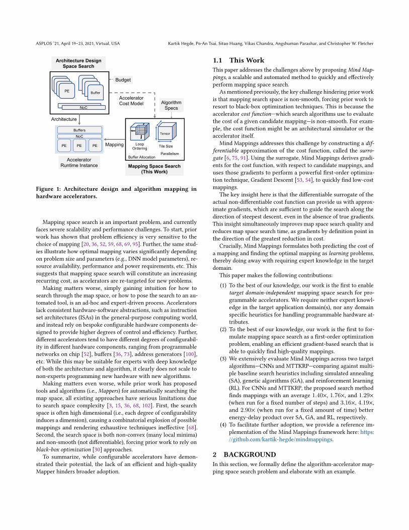
Figure 2: A basic hardware accelerator with𝑀 processing el-ements, on-chip buffer with 𝑁 banks, and a NoC.

That is, we complete the 1D-Conv for an 𝑅𝑡 chunk of F at a time,adding an outer loop over the number of tiles 𝑅𝑐 . This loop nestis therefore written as 𝑅𝑐 →𝑊 → 𝑅𝑡 . Beyond tiling, we can de-scribe parallelism in the computation by conceptually pre-pendingparallel before a given loop(s), indicating that iterations of thatloop can run in parallel.

An example target accelerator for the 1D-Conv algorithm isdepicted in Figure 2. At a high-level, it has𝑀 processing elements,an on-chip buffer with 𝑁 banks allocatable to different tensors atbank granularity, a flexible NoC that can be optimized for differentcommunication patterns such as broadcast, unicast, etc.

Let us assume that the accelerator’s programmable attributesare:

(1) 𝑃0 = R3: a 3-tuple indicating the percentage of banks allo-cated to each of I, O, and F.

(2) 𝑃1 = Z3+: a 3-tuple representing the tile shape of I, O, andF to be fetched from DRAM.1 The + is to facilitate multiplelevels of tiling, if applicable.

(3) 𝑃2 = {𝑊 → 𝑅, 𝑅 →𝑊 }: loop order for the untiled 1D-Convalgorithm represented in Code 1. To support more loopslevels due to tiling (as in Code 2), we add additional tiledloop orders to 𝑃2 (e.g., 𝑅𝑐 →𝑊 → 𝑅𝑡 ).

(4) 𝑃3 = Z+: the loop bound for each loop, e.g., 𝑅𝑐 ,𝑊 +𝑅 − 1, 𝑅𝑡in Code 2. Note, we write this attribute explicitly for clarity.In this example, loop bound can be inferred from the currentassignment to 𝑃1 and 𝑃2.

(5) 𝑃4 = {unicast, multicast, broadcast}3: NoC communicat-ing patterns for each of the 3 tensors.

(6) 𝑃5 = Z+: Amount of parallelism per PE for each loop level.Mapping Space. Given the above, one can construct a mapping

space𝑀𝑎,𝑝 for the accelerator and specific 1D-Conv problem (i.e.,the specific setting of𝑊 and 𝑅). The accelerator has 𝐷 = 6 pro-grammable attributes and the mapping space size is bounded by thesize of the Cartesian product of assignments to each programmableattribute. As discussed in Section 2.1, the mapping space size willbe smaller than this upper bound, as some complete assignments toprogrammable attributes are invalid, e.g., 𝑅𝑡 < 𝑅 must hold since𝑅𝑡 is a tile of 𝑅.

1Note that in 1D-Conv, tiles are 1-dimensional. Hence, shape is representable as ascalar.

Cost Function. In the above example, the cost of a mapping𝑓 (𝑚) is defined as energy ∗ delay. This can be obtained by simu-lators or analytical models that represent the actual hardware orusing the actual hardware itself. For example, Timeloop [68] (whichwe use in our evaluation) is a tool that can calculate mapping costfor algorithms representable as affine loop nests (e.g., convolutions).

3.1 Challenges in Mapping Space Search

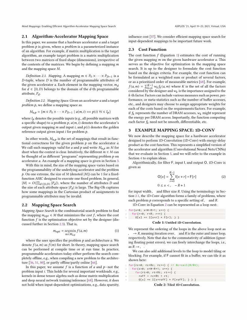
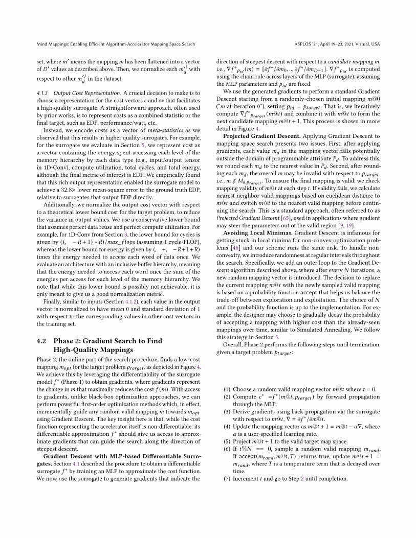
Figure 3: Cost surface plot for the accelerator we evaluatein Section 5 for CNNs. Darker red indicates higher EDP, anddarker blue indicates lower EDP. Mind Mappings approxi-mates this non-smooth surface with a differentiable surro-gate to enable gradient-based optimization.

A major challenge in mapping space search is the nature of costfunction 𝑓 , which is non-convex and non-smooth. For example,consider the 1D-Conv example from the previous sub-section. Thecost of a mapping 𝑓 (𝑚) is influenced by the various programmableattributes 𝑃𝑑 in subtle ways. For example, consider 𝑃0, the attributethat represents buffer allocation for each operand/result tensor I,O, and F. If the F tensor is 1 KB in size and allocation falls shortof 1 KB, the mapping cost will see a significant energy bump asvalid mappings will be forced to tile F, requiring some operand(s)to be re-fetched multiple times to fully compute O. In other words,seemingly minor changes to mapping𝑚 can result in non-smoothchanges to the overall cost 𝑓 (𝑚).

To illustrate this, Figure 3 plots the cost surface for the pro-grammable accelerator running Convolutional Neural Network(CNN) layers that we evaluate in Section 5. In the figure, the 𝑥-and 𝑦-axis represent different choices of tile sizes for two differentinput tensors, while the 𝑧-axis represents the cost 𝑓 in terms of theenergy-delay product (EDP). Evident from the plot, the search spaceis spiky and non-smooth in nature. Due to this, obtaining usefulstatistics such as the gradients (first-order), Hessians (second-order)of the search space is not possible, requiring the search for optimalmapping (Equation 1) to use black-box optimization approachessuch as Simulated Annealing [45], Genetic Algorithms [89], etc.Making matters worse, the search space is clearly non-convex, i.e.,


many local minima, making the search even harder. Given the hu-mongous search space size (≈ 1025 in this example), black-boxoptimization approaches struggle to find high quality mappings infew iterations.

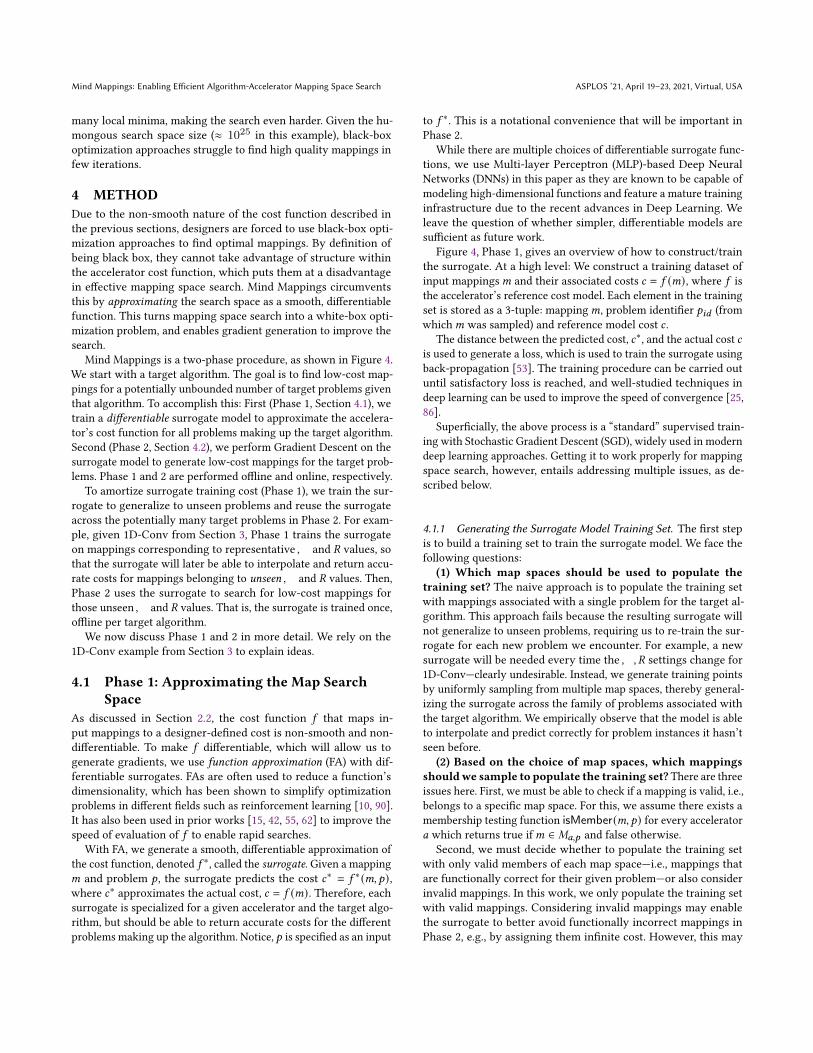
4 METHODDue to the non-smooth nature of the cost function described inthe previous sections, designers are forced to use black-box opti-mization approaches to find optimal mappings. By definition ofbeing black box, they cannot take advantage of structure withinthe accelerator cost function, which puts them at a disadvantagein effective mapping space search. Mind Mappings circumventsthis by approximating the search space as a smooth, differentiablefunction. This turns mapping space search into a white-box opti-mization problem, and enables gradient generation to improve thesearch.

Mind Mappings is a two-phase procedure, as shown in Figure 4.We start with a target algorithm. The goal is to find low-cost map-pings for a potentially unbounded number of target problems giventhat algorithm. To accomplish this: First (Phase 1, Section 4.1), wetrain a differentiable surrogate model to approximate the accelera-tor’s cost function for all problems making up the target algorithm.Second (Phase 2, Section 4.2), we perform Gradient Descent on thesurrogate model to generate low-cost mappings for the target prob-lems. Phase 1 and 2 are performed offline and online, respectively.

To amortize surrogate training cost (Phase 1), we train the sur-rogate to generalize to unseen problems and reuse the surrogateacross the potentially many target problems in Phase 2. For exam-ple, given 1D-Conv from Section 3, Phase 1 trains the surrogateon mappings corresponding to representative𝑊 and 𝑅 values, sothat the surrogate will later be able to interpolate and return accu-rate costs for mappings belonging to unseen𝑊 and 𝑅 values. Then,Phase 2 uses the surrogate to search for low-cost mappings forthose unseen𝑊 and 𝑅 values. That is, the surrogate is trained once,offline per target algorithm.

We now discuss Phase 1 and 2 in more detail. We rely on the1D-Conv example from Section 3 to explain ideas.

4.1 Phase 1: Approximating the Map SearchSpace

As discussed in Section 2.2, the cost function 𝑓 that maps in-put mappings to a designer-defined cost is non-smooth and non-differentiable. To make 𝑓 differentiable, which will allow us togenerate gradients, we use function approximation (FA) with dif-ferentiable surrogates. FAs are often used to reduce a function’sdimensionality, which has been shown to simplify optimizationproblems in different fields such as reinforcement learning [10, 90].It has also been used in prior works [15, 42, 55, 62] to improve thespeed of evaluation of 𝑓 to enable rapid searches.

With FA, we generate a smooth, differentiable approximation ofthe cost function, denoted 𝑓 ∗, called the surrogate. Given a mapping𝑚 and problem 𝑝 , the surrogate predicts the cost 𝑐∗ = 𝑓 ∗ (𝑚, 𝑝),where 𝑐∗ approximates the actual cost, 𝑐 = 𝑓 (𝑚). Therefore, eachsurrogate is specialized for a given accelerator and the target algo-rithm, but should be able to return accurate costs for the differentproblems making up the algorithm. Notice, 𝑝 is specified as an input

to 𝑓 ∗. This is a notational convenience that will be important inPhase 2.

While there are multiple choices of differentiable surrogate func-tions, we use Multi-layer Perceptron (MLP)-based Deep NeuralNetworks (DNNs) in this paper as they are known to be capable ofmodeling high-dimensional functions and feature a mature traininginfrastructure due to the recent advances in Deep Learning. Weleave the question of whether simpler, differentiable models aresufficient as future work.

Figure 4, Phase 1, gives an overview of how to construct/trainthe surrogate. At a high level: We construct a training dataset ofinput mappings𝑚 and their associated costs 𝑐 = 𝑓 (𝑚), where 𝑓 isthe accelerator’s reference cost model. Each element in the trainingset is stored as a 3-tuple: mapping𝑚, problem identifier 𝑝𝑖𝑑 (fromwhich𝑚 was sampled) and reference model cost 𝑐 .

The distance between the predicted cost, 𝑐∗, and the actual cost 𝑐is used to generate a loss, which is used to train the surrogate usingback-propagation [53]. The training procedure can be carried outuntil satisfactory loss is reached, and well-studied techniques indeep learning can be used to improve the speed of convergence [25,86].

Superficially, the above process is a “standard” supervised train-ing with Stochastic Gradient Descent (SGD), widely used in moderndeep learning approaches. Getting it to work properly for mappingspace search, however, entails addressing multiple issues, as de-scribed below.

4.1.1 Generating the Surrogate Model Training Set. The first stepis to build a training set to train the surrogate model. We face thefollowing questions:

(1) Which map spaces should be used to populate thetraining set? The naive approach is to populate the training setwith mappings associated with a single problem for the target al-gorithm. This approach fails because the resulting surrogate willnot generalize to unseen problems, requiring us to re-train the sur-rogate for each new problem we encounter. For example, a newsurrogate will be needed every time the𝑊,𝑅 settings change for1D-Conv—clearly undesirable. Instead, we generate training pointsby uniformly sampling from multiple map spaces, thereby general-izing the surrogate across the family of problems associated withthe target algorithm. We empirically observe that the model is ableto interpolate and predict correctly for problem instances it hasn’tseen before.

(2) Based on the choice of map spaces, which mappingsshouldwe sample to populate the training set? There are threeissues here. First, we must be able to check if a mapping is valid, i.e.,belongs to a specific map space. For this, we assume there exists amembership testing function isMember(𝑚, 𝑝) for every accelerator𝑎 which returns true if𝑚 ∈ 𝑀𝑎,𝑝 and false otherwise.

Second, we must decide whether to populate the training setwith only valid members of each map space—i.e., mappings thatare functionally correct for their given problem—or also considerinvalid mappings. In this work, we only populate the training setwith valid mappings. Considering invalid mappings may enablethe surrogate to better avoid functionally incorrect mappings inPhase 2, e.g., by assigning them infinite cost. However, this may


Trainable Non-Trainable

UniformRandom Sampling

Surrogate Model𝑐∗ = 𝑓∗(𝑚, 𝑝"#)

𝑚Accelerator Cost Model

𝑐

𝑚, 𝑝!"

𝑝!"

𝑐

𝑐∗

Loss

𝜕𝐿𝜕𝑤

TrainingSet

Map Spaces

Surrogate Model𝑐∗ = 𝑓∗(𝑚, 𝑝"#)

𝑚@𝑡

𝑝$%&'($

Gradients via Surrogate

𝑐∗

𝛻 =𝜕𝑓∗

𝜕𝑚

Random Initial Mapping

𝑚@𝑡+ 1 = 𝑚@𝑡 − 𝛼𝛻

𝑚@0

Phase 1 Phase 2

Figure 4: Mind Mappings search procedure. Phase 1: Training the surrogate model 𝑐∗ = 𝑓 ∗ (𝑚, 𝑝𝑖𝑑 ) based on (mapping, problemid, cost) tuples (𝑚, 𝑝𝑖𝑑 , 𝑐). DNN (surrogate) weights𝑤 are trained with back-propagation. Phase 2: Given a target problem 𝑝𝑡𝑎𝑟𝑔𝑒𝑡 ,use the trained surrogate model to iteratively guide a random initial mapping𝑚@0 (“mapping at search iteration 0”) towardsan optimal mapping𝑚𝑜𝑝𝑡 . In each iteration,𝑚@𝑡 is updated using back-propagation with a gradient ∇ of 𝑓 ∗ based on𝑚@𝑡 witha learning rate 𝛼 . The trained model weights𝑤 and the target problem 𝑝𝑡𝑎𝑟𝑔𝑒𝑡 are held constant in this phase.

face implementation challenges such as exploding gradients andslow convergence [70].

Third, we need to decide on a sampling strategy to sample fromeach map space. One option, which we use in this work, is tosample uniformly at random. Specifically, given a problem 𝑝 , wesample from the associated map space𝑀𝑎,𝑝 uniformly to generate amapping and re-sample if the mapping is not valid (see above). Thisensures a reasonable representation of the map space, but mightsuffer from under-sampling from regions that are more importantfrom a training perspective. Other advanced sampling methods canbe used, such as sampling from a probability distribution trainedto maximize the amount of learning per sample [60]. As seen fromour evaluation (Section 5), uniform random sampling facilitatestraining well and therefore we leave improved sampling methodsto future work.

(3) How to uniquely associate each mapping 𝑚 with itsmap space𝑀𝑎,𝑝? It is possible to have the samemapping𝑚 presentin multiple map spaces, where each mapping instance has a dif-ferent cost 𝑐 . Therefore, to ensure correct generalization of thesurrogate across different problems for the given algorithm, wemust uniquely identify each mapping in the training set with itsmap space. For this, we need to tag each mapping𝑚, added to thetraining set, with a problem identifier 𝑝𝑖𝑑 , unique to the map spaceassociated with its problem 𝑝 . In this paper, we encode each 𝑝𝑖𝑑 asthe specific parameterization of the problem, e.g., a tuple indicat-ing the𝑊,𝑅 values associated with the problem for the 1D-Convalgorithm (Section 3).

(4) How to calculate cost per mapping? To train the surro-gate, we require a reference cost 𝑐 = 𝑓 (𝑚) that can be used tocalculate the loss w.r.t. surrogate’s predicted cost 𝑐∗. This can beestimated via running the problem with mapping𝑚 on the targethardware or using a cost function estimator such as those described

in Section 2.3. As this is a one-time, offline procedure that gener-alizes over different problems for the target algorithm, its cost isamortized over multiple mapping space searches performed usingthis surrogate.

We now describe input mapping vector and output cost rep-resentation. We describe ideas and challenges here. The concreterepresentations we use for our evaluation are detailed in Section 5.5.

4.1.2 Input Mapping Representation. As described in Section 2.1,the mapping vector𝑚 is a 𝐷-tuple consisting of the accelerator’sprogrammable attributes, which needs to be converted to a repre-sentation that can be used to train the surrogate. There are twoissues here. First, while each programmable attribute 𝑃𝑑 can havedifferent representations, e.g., vector, integer, float, boolean, etc.,the input to the surrogate needs to be a single vector of floats. Weresolve this by converting each attribute to a scalar or a vectorof floats, flattening multiple vectors into a final mapping vectoras needed. For example, 𝑃4 in 1D-Conv (Section 3) has 3 discretechoices, which can be converted to a vector of 3 floats which are one-hot encoded. The choice of float for the mapping vector datatypeisn’t fundamental; in what follows, we refer to each float/elementin the mapping vector as a value.

Second, in some cases, it may be desirable to have variable-length mapping vectors for different problems (e.g., to encode vari-able levels of tiling), but the input vector to the surrogate is oftenfixed (e.g., as in a Multi-layer Perceptron). While we deal withfixed-dimensionality mappings in this work, the above can be eas-ily handled via embeddings [63], a widely used method to dealwith different input lengths in areas such as Natural LanguageProcessing and Recommendation Systems.

Finally, we normalize each value in eachmapping to have mean 0,standard deviation 1—in a process akin to input whitening [25, 50].That is, let𝑚′𝑖

𝑑be the 𝑑-th value in the 𝑖-th mapping in the training


set, where𝑚′ means the mapping𝑚 has been flattened into a vectorof 𝐷 ′ values as described above. Then, we normalize each𝑚′𝑖

𝑑with

respect to other𝑚′𝑗𝑑

in the dataset.

4.1.3 Output Cost Representation. A crucial decision to make is tochoose a representation for the cost vectors 𝑐 and 𝑐∗ that facilitatesa high quality surrogate. A straightforward approach, often usedby prior works, is to represent costs as a combined statistic or thefinal target, such as EDP, performance/watt, etc.

Instead, we encode costs as a vector of meta-statistics as weobserved that this results in higher quality surrogates. For example,for the surrogate we evaluate in Section 5, we represent cost asa vector containing the energy spent accessing each level of thememory hierarchy by each data type (e.g., input/output tensorin 1D-Conv), compute utilization, total cycles, and total energy,although the final metric of interest is EDP. We empirically foundthat this rich output representation enabled the surrogate model toachieve a 32.8× lower mean-square error to the ground truth EDP,relative to surrogates that output EDP directly.

Additionally, we normalize the output cost vector with respectto a theoretical lower bound cost for the target problem, to reducethe variance in output values. We use a conservative lower boundthat assumes perfect data reuse and perfect compute utilization. Forexample, for 1D-Conv from Section 3, the lower bound for cycles isgiven by ((𝑊 − 𝑅 + 1) ∗ 𝑅)/𝑚𝑎𝑥_𝑓 𝑙𝑜𝑝𝑠 (assuming 1 cycle/FLOP),whereas the lower bound for energy is given by (𝑊 +𝑊 −𝑅 +1+𝑅)times the energy needed to access each word of data once. Weevaluate an architecture with an inclusive buffer hierarchy, meaningthat the energy needed to access each word once the sum of theenergies per access for each level of the memory hierarchy. Wenote that while this lower bound is possibly not achievable, it isonly meant to give us a good normalization metric.

Finally, similar to inputs (Section 4.1.2), each value in the outputvector is normalized to have mean 0 and standard deviation of 1with respect to the corresponding values in other cost vectors inthe training set.

4.2 Phase 2: Gradient Search to FindHigh-Quality Mappings

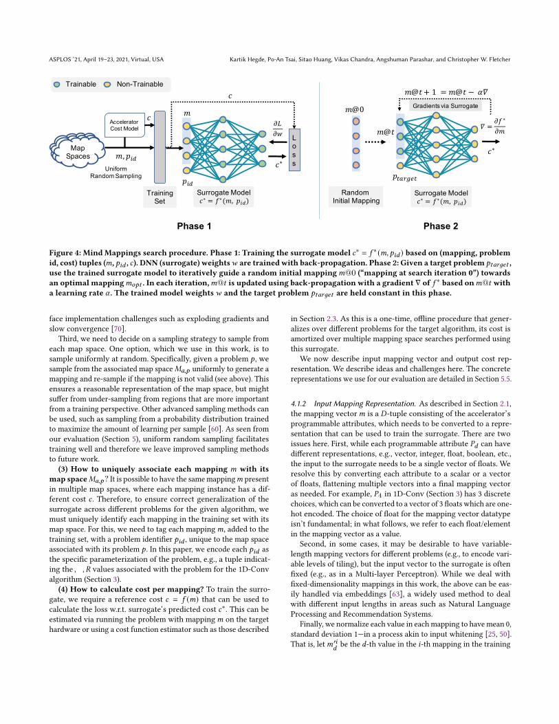
Phase 2, the online part of the search procedure, finds a low-costmapping𝑚𝑜𝑝𝑡 for the target problem 𝑝𝑡𝑎𝑟𝑔𝑒𝑡 , as depicted in Figure 4.We achieve this by leveraging the differentiability of the surrogatemodel 𝑓 ∗ (Phase 1) to obtain gradients, where gradients representthe change in𝑚 that maximally reduces the cost 𝑓 (𝑚). With accessto gradients, unlike black-box optimization approaches, we canperform powerful first-order optimization methods which, in effect,incrementally guide any random valid mapping𝑚 towards𝑚𝑜𝑝𝑡using Gradient Descent. The key insight here is that, while the costfunction representing the accelerator itself is non-differentiable, itsdifferentiable approximation 𝑓 ∗ should give us access to approx-imate gradients that can guide the search along the direction ofsteepest descent.

Gradient Descent with MLP-based Differentiable Surro-gates. Section 4.1 described the procedure to obtain a differentiablesurrogate 𝑓 ∗ by training an MLP to approximate the cost function.We now use the surrogate to generate gradients that indicate the

direction of steepest descent with respect to a candidate mapping𝑚,i.e., ∇𝑓 ∗𝑝𝑖𝑑 (𝑚) = [𝜕𝑓 ∗/𝜕𝑚0, .., 𝜕𝑓

∗/𝜕𝑚𝐷−1]. ∇𝑓 ∗𝑝𝑖𝑑 is computedusing the chain rule across layers of the MLP (surrogate), assumingthe MLP parameters and 𝑝𝑖𝑑 are fixed.

We use the generated gradients to perform a standard GradientDescent starting from a randomly-chosen initial mapping 𝑚@0(“𝑚 at iteration 0”), setting 𝑝𝑖𝑑 = 𝑝𝑡𝑎𝑟𝑔𝑒𝑡 . That is, we iterativelycompute ∇𝑓 ∗𝑝𝑡𝑎𝑟𝑔𝑒𝑡 (𝑚@𝑡) and combine it with𝑚@𝑡 to form thenext candidate mapping𝑚@𝑡 + 1. This process is shown in moredetail in Figure 4.

Projected Gradient Descent. Applying Gradient Descent tomapping space search presents two issues. First, after applyinggradients, each value𝑚𝑑 in the mapping vector falls potentiallyoutside the domain of programmable attribute 𝑃𝑑 . To address this,we round each𝑚𝑑 to the nearest value in 𝑃𝑑 . Second, after round-ing each𝑚𝑑 , the overall𝑚 may be invalid with respect to 𝑝𝑡𝑎𝑟𝑔𝑒𝑡 ,i.e.,𝑚 ̸∈ 𝑀𝑎,𝑝𝑡𝑎𝑟𝑔𝑒𝑡 . To ensure the final mapping is valid, we checkmapping validity of𝑚@𝑡 at each step 𝑡 . If validity fails, we calculatenearest neighbor valid mappings based on euclidean distance to𝑚@𝑡 and switch𝑚@𝑡 to the nearest valid mapping before contin-uing the search. This is a standard approach, often referred to asProjected Gradient Descent [65], used in applications where gradientmay steer the parameters out of the valid region [9, 19].

Avoiding Local Minimas. Gradient Descent is infamous forgetting stuck in local minima for non-convex optimization prob-lems [46] and our scheme runs the same risk. To handle non-convexity, we introduce randomness at regular intervals throughoutthe search. Specifically, we add an outer loop to the Gradient De-scent algorithm described above, where after every 𝑁 iterations, anew random mapping vector is introduced. The decision to replacethe current mapping𝑚@𝑡 with the newly sampled valid mappingis based on a probability function accept that helps us balance thetrade-off between exploration and exploitation. The choice of 𝑁and the probability function is up to the implementation. For ex-ample, the designer may choose to gradually decay the probabilityof accepting a mapping with higher cost than the already-seenmappings over time, similar to Simulated Annealing. We followthis strategy in Section 5.

Overall, Phase 2 performs the following steps until termination,given a target problem 𝑝𝑡𝑎𝑟𝑔𝑒𝑡 :

(1) Choose a random valid mapping vector𝑚@𝑡 where 𝑡 = 0.(2) Compute 𝑐∗ =𝑓 ∗ (𝑚@𝑡, 𝑝𝑡𝑎𝑟𝑔𝑒𝑡 ) by forward propagation

through the MLP.(3) Derive gradients using back-propagation via the surrogate

with respect to𝑚@𝑡 , ∇ = 𝜕𝑓 ∗/𝜕𝑚@𝑡 .(4) Update the mapping vector as𝑚@𝑡 + 1 =𝑚@𝑡 − 𝛼∇, where

𝛼 is a user-specified learning rate.(5) Project𝑚@𝑡 + 1 to the valid target map space.(6) If 𝑡%𝑁 == 0, sample a random valid mapping 𝑚𝑟𝑎𝑛𝑑 .

If accept(𝑚𝑟𝑎𝑛𝑑 ,𝑚@𝑡,𝑇 ) returns true, update 𝑚@𝑡 + 1 =

𝑚𝑟𝑎𝑛𝑑 , where 𝑇 is a temperature term that is decayed overtime.

(7) Increment 𝑡 and go to Step 2 until completion.


5 EVALUATIONWe now evaluate Mind Mappings. We design representative flexiblehardware accelerators using Timeloop [68] and search throughtheir map spaces in the context of two target algorithms, whilecomparing against several other search methods.

5.1 Experimental Setup5.1.1 Algorithms. We evaluate Mind Mappings by evaluating twotarget algorithms, Convolutional Neural Networks (CNN) and Ma-tricized tensor times Khatri-Rao product (MTTKRP). We evalu-ate two target algorithms to demonstrate generality, and selectedthese two in particular given the ongoing effort in the archi-tecture community to build efficient hardware accelerators forCNNs [4, 18, 20, 26, 38, 69, 101] and MTTKRP [37, 87]. CNN lay-ers feature similar, but higher-dimensional, computations as our1D-Conv example from Section 3.

CNN-Layer. CNNs have seen widespread success in modernDeep Learning applications such as image recognition, video an-alytics etc. A CNN layer takes 𝑁 2D images of resolution𝑊 × 𝐻with 𝐶 channels and 𝐾 filters of resolution 𝑅 × 𝑆 and produces anoutput of size 𝑋 × 𝑌 with 𝐾 channels. Value of 𝑋 and 𝑌 can becalculated from𝑊 and 𝐻 respectively as (𝑊 − 𝑅 + 1)/𝑠𝑡𝑟𝑖𝑑𝑒 and(𝐻 − 𝑆 + 1)/𝑠𝑡𝑟𝑖𝑑𝑒 , respectively. Mathematically, a CNN Layer isgiven by Equation 3.

O[(𝑘, 𝑥,𝑦)] =𝐶−1∑︁𝑐=0

𝑅−1∑︁𝑟=0

𝑆−1∑︁𝑠=0

F[(𝑘, 𝑐, 𝑟, 𝑠)] ∗ I[(𝑐, 𝑥 + 𝑟,𝑦 + 𝑠)] (3)

0 ≤ 𝑘 < 𝐾, 0 ≤ 𝑥 <𝑊 − 𝑅 + 1, 0 ≤ 𝑦 < 𝐻 − 𝑆 + 1

MTTKRP.MTTKRP [83] is a key kernel in Tensor Algebra thatis a bottleneck in applications such as tensor decompositions [47],alternating least squares [11], Jacobian estimation [93], etc. MT-TKRP takes a 3D tensor 𝐴, and matrices 𝐵 & 𝐶 to produce andoutput matrix by contracting across two dimensions, as describedin Equation 4.

O[(𝑖, 𝑗)] =𝐾∑︁𝑘=0

𝐿∑︁𝑙=0

𝐴[(𝑖, 𝑘, 𝑙)] ∗ 𝐵 [(𝑘, 𝑗)] ∗𝐶 [(𝑙, 𝑗)] (4)

0 ≤ 𝑖 < 𝐼 , 0 ≤ 𝑗 < 𝐽

Table 1: Target problems for each target algorithm.

CNN/MTTKRP N/I K/J H,W/K R,S C/LResNet Conv_3 16 128 28 3 128ResNet Conv_4 16 256 14 3 256Inception Conv_2 32 192 56 3 192VGG Conv_2 16 128 112 3 64

AlexNet Conv_2 8 256 27 5 96AlexNet Conv_4 8 384 13 3 384MTTKRP_0 128 1024 4096 - 2048MTTKRP_1 2048 4096 1024 - 128

Table 1 shows the target problems we evaluated in Phase 2 foreach algorithm. Specifically, we chose layers from popular networks

such as ResNet [35], VGG [82], AlexNet [50], and Inception-V3 [92]and representative matrix shapes (tall and skinny [85]) for MT-TKRP.

5.1.2 Hardware Accelerators. We model the programmable hard-ware accelerator using Timeloop [68], which uses an analyticalcost model to provide a high-fidelity cost estimation for hardwareaccelerators that implement affine loopnests.

The hardware accelerators we evaluate for both algorithms havethe same memory hierarchy, namely a two-level hierarchy with512 KB of shared buffer and 64 KB of private buffer for each of 256processing elements (PEs). Buffers are banked and can be flexiblyallocated to store any algorithm operand/partial result (tensorsin the case of our target algorithms). Each level of the memoryhierarchy is coupled with control and address generation logic tosupport any loop order and tile size (similar to [36]). The Network-on-Chip (NoC) provides parallelism across the PEs along any com-bination of problem dimensions.

For each algorithm, we further specialize the datapath and con-trol logic in PEs and the rest of the accelerator. For CNN-Layer,PEs can consume 2 operands to produce 1 output per cycle, whilefor MTTKRP, PEs consume 3 operands to produce 1 output percycle. We assume the accelerator runs at 1 GHz and that the designobjective is to minimize the energy-delay product (EDP) to evaluatea problem.

5.1.3 Map Spaces. Given the accelerator architecture 𝑎 and targetproblem 𝑝 , each mapping 𝑚 ∈ 𝑀𝑎,𝑝 (Section 4.1.2) is defined bythe following programmable attributes for CNN-Layer/MTTKRP,typical in recent accelerators [20, 36, 38, 52, 59, 69].

(1) Tiling: The tile sizes for each dimension (7/4) for each ofthe 3 levels in the memory hierarchy (DRAM, L2, and L1).(21/12 attributes for CNN-Layer and MTTKRP, respectively.)

(2) Parallelism: The degree of parallelism for each dimensionacross the PEs. (7/4 attributes.)

(3) Loop Orders: The ordering for each dimensions for each ofthe 3 memory hierarchies. (3/3 attributes.)

(4) Buffer Allocation: The allocation of banks for each ten-sor (3/4) for 2 levels of on-chip memory hierarchy. (6/8 at-tributes.)

These attributes induce a map space that is too large to exhaus-tively search. For example, themap space size for the ResNet Conv_4layer (CNN-Layer) is ≈ 1025 valid mappings.

To characterize the search space, we sampled 1 M samples fromeach of the map spaces implied by Table 1 and computed the energyof each sample, which resulted in a (𝑚𝑒𝑎𝑛, 𝑠𝑡𝑑) of (44.2, 231.4),(48.0, 51.2) for CNN-Layer/MTTKRP respectively, when energywas normalized to a theoretical lower-bound energy for the givenproblem.

5.2 Search Methods and Comparison MetricsWe compare Mind Mappings with following popular search meth-ods used in prior work.

(1) Algorithmic Minimum: Refers to the theoretical lower-bound, possibly unachievable.

(2) Simulated Annealing (SA): A popular black-box optimiza-tion method [45].


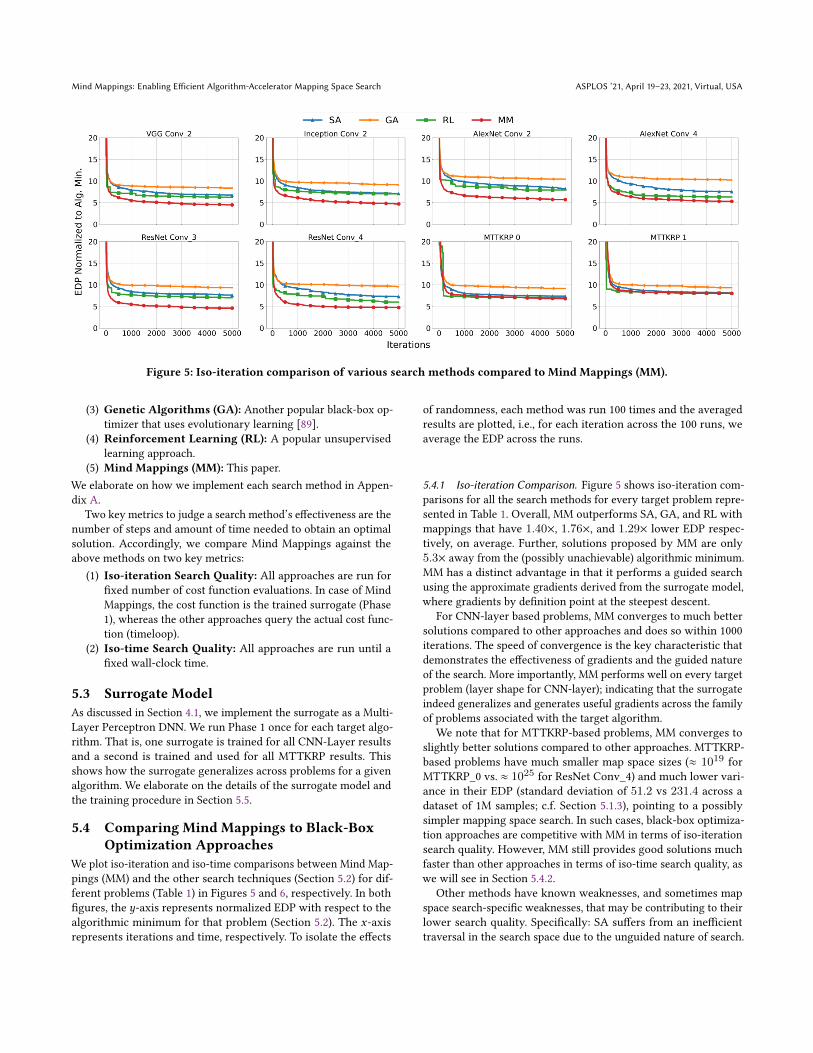
Figure 5: Iso-iteration comparison of various search methods compared to Mind Mappings (MM).

(3) Genetic Algorithms (GA): Another popular black-box op-timizer that uses evolutionary learning [89].

(4) Reinforcement Learning (RL): A popular unsupervisedlearning approach.

(5) Mind Mappings (MM): This paper.We elaborate on how we implement each search method in Appen-dix A.

Two key metrics to judge a search method’s effectiveness are thenumber of steps and amount of time needed to obtain an optimalsolution. Accordingly, we compare Mind Mappings against theabove methods on two key metrics:

(1) Iso-iteration Search Quality: All approaches are run forfixed number of cost function evaluations. In case of MindMappings, the cost function is the trained surrogate (Phase1), whereas the other approaches query the actual cost func-tion (timeloop).

(2) Iso-time Search Quality: All approaches are run until afixed wall-clock time.

5.3 Surrogate ModelAs discussed in Section 4.1, we implement the surrogate as a Multi-Layer Perceptron DNN. We run Phase 1 once for each target algo-rithm. That is, one surrogate is trained for all CNN-Layer resultsand a second is trained and used for all MTTKRP results. Thisshows how the surrogate generalizes across problems for a givenalgorithm. We elaborate on the details of the surrogate model andthe training procedure in Section 5.5.

5.4 Comparing Mind Mappings to Black-BoxOptimization Approaches

We plot iso-iteration and iso-time comparisons between Mind Map-pings (MM) and the other search techniques (Section 5.2) for dif-ferent problems (Table 1) in Figures 5 and 6, respectively. In bothfigures, the 𝑦-axis represents normalized EDP with respect to thealgorithmic minimum for that problem (Section 5.2). The 𝑥-axisrepresents iterations and time, respectively. To isolate the effects

of randomness, each method was run 100 times and the averagedresults are plotted, i.e., for each iteration across the 100 runs, weaverage the EDP across the runs.

5.4.1 Iso-iteration Comparison. Figure 5 shows iso-iteration com-parisons for all the search methods for every target problem repre-sented in Table 1. Overall, MM outperforms SA, GA, and RL withmappings that have 1.40×, 1.76×, and 1.29× lower EDP respec-tively, on average. Further, solutions proposed by MM are only5.3× away from the (possibly unachievable) algorithmic minimum.MM has a distinct advantage in that it performs a guided searchusing the approximate gradients derived from the surrogate model,where gradients by definition point at the steepest descent.

For CNN-layer based problems, MM converges to much bettersolutions compared to other approaches and does so within 1000iterations. The speed of convergence is the key characteristic thatdemonstrates the effectiveness of gradients and the guided natureof the search. More importantly, MM performs well on every targetproblem (layer shape for CNN-layer); indicating that the surrogateindeed generalizes and generates useful gradients across the familyof problems associated with the target algorithm.

We note that for MTTKRP-based problems, MM converges toslightly better solutions compared to other approaches. MTTKRP-based problems have much smaller map space sizes (≈ 1019 forMTTKRP_0 vs. ≈ 1025 for ResNet Conv_4) and much lower vari-ance in their EDP (standard deviation of 51.2 vs 231.4 across adataset of 1M samples; c.f. Section 5.1.3), pointing to a possiblysimpler mapping space search. In such cases, black-box optimiza-tion approaches are competitive with MM in terms of iso-iterationsearch quality. However, MM still provides good solutions muchfaster than other approaches in terms of iso-time search quality, aswe will see in Section 5.4.2.

Other methods have known weaknesses, and sometimes mapspace search-specific weaknesses, that may be contributing to theirlower search quality. Specifically: SA suffers from an inefficienttraversal in the search space due to the unguided nature of search.


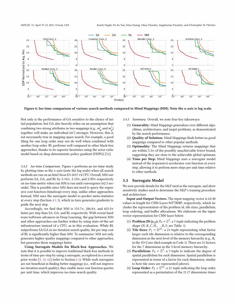
Figure 6: Iso-time comparison of various search methods compared to Mind Mappings (MM). Note the x-axis is log scale.

Not only is the performance of GA sensitive to the choice of ini-tial population, but GA also heavily relies on an assumption thatcombining two strong attributes in two mappings (e.g.,𝑚𝑖

𝑑and𝑚 𝑗

𝑑)

together will make an individual (𝑚′) stronger. However, this isnot necessarily true in mapping space search. For example, a goodtiling for one loop order may not do well when combined withanother loop order. RL performs well compared to other black-boxapproaches, thanks to its superior heuristics using the actor-criticmodel based on deep deterministic policy gradient (DDPG) [56].

5.4.2 Iso-time Comparison. Figure 6 performs an iso-time studyby plotting time as the 𝑥-axis (note the log scale) when all searchmethods are run on an Intel Xeon E5-2637 v4 CPU. Overall, MM out-performs SA, GA, and RL by 3.16×, 4.19×, and 2.90× respectivelyon iso-time metric when run MM is run until convergence (62.5 sec-onds). This is possible since MM does not need to query the expen-sive cost function (timeloop) every step, unlike other approaches.Instead, MM uses the surrogate model to predict meta-statisticsat every step (Section 4.1.3), which in turn generates gradients toguide the next step.

Accordingly, we find that MM is 153.7×, 286.8×, and 425.5×faster per step than SA, GA, and RL respectively. With recent hard-ware/software advances in Deep Learning, the gap between MMand other approaches can further widen by using state-of-the-artinfrastructure instead of a CPU, as in this evaluation. While RLoutperforms SA/GA in iso-iteration search quality, the per step costof RL is significantly higher than MM. To summarize: MM not onlygenerates higher-quality mappings compared to other approaches,but generates those mappings faster.

Using Surrogate Models for Black-box Approaches. Wenote that it is possible to improve traditional black-box methods interms of time-per-step by using a surrogate, as explored in a severalprior works [3, 15, 62] (refer to Section 6.1). While such surrogatesare not beneficial in finding better mappings (i.e., will not improveiso-iteration search quality), they enable more cost function queriesper unit time, which improves iso-time search quality.

5.4.3 Summary. Overall, we note four key takeaways:(1) Generality:Mind Mappings generalizes over different algo-

rithms, architectures, and target problems, as demonstratedby the search performance.

(2) Quality of Solution:Mind Mappings finds better/as goodmappings compared to other popular methods.

(3) Optimality: The Mind Mappings returns mappings thatare within 5.3× of the possibly unachievable lower bound,suggesting they are close to the achievable global optimum.

(4) Time per Step: Mind Mappings uses a surrogate modelinstead of the (expensive) accelerator cost function at everystep, allowing it to perform more steps per unit time relativeto other methods.

5.5 Surrogate ModelWe now provide details for the MLP used as the surrogate, and showsensitivity studies used to determine the MLP’s training procedureand architecture.

Input and Output Vectors. The input mapping vector is 62/40values in length for CNN-Layer/MTTKRP, respectively, which in-cludes the representation of the problem id, tile sizes, parallelism,loop ordering, and buffer allocations. We elaborate on the inputvector representation for CNN-layer below.

(1) Problem ID (𝑝𝑖𝑑 ): 𝑃0 = Z7: a 7-tuple indicating the problemshape (𝑁,𝐾,𝐶, 𝐻,𝑊 , 𝑅, 𝑆 ; see Table 1).

(2) Tile Sizes: 𝑃1 = R21: a 21-tuple representing what factorlarger each tile dimension is relative to the correspondingdimension in the next level of the memory hierarchy (e.g., 𝑅𝑐in the 1D-Conv tiled example in Code 2). There are 21 factors,for the 7 dimensions in the 3-level memory hierarchy.

(3) Parallelism: 𝑃2 = Z7: a 7-tuple to indicate the degree ofspatial parallelism for each dimension. Spatial parallelism isrepresented in terms of a factor for each dimension, similarto how tile sizes are represented (above).

(4) Loop Order: 𝑃3 = Z21: a 21-tuple indicating the loop order,represented as a permutation of the 21 (7 dimensions times


(a) Training and test loss. (b) Choosing a loss function. (c) Sensitivity to training set size.

Figure 7: Experiments to determine the DNN topology and the loss function.

3 levels of memory) loops. For example, in 1D-Conv𝑊 → 𝑅

is represented as [0, 1], and 𝑅 →𝑊 is 1, 0.(5) Buffer Allocation: 𝑃4 = R6: a 6-tuple indicating the per-

centage of banks in each of the 2 levels of on-chip memoryallocated to each of the 3 tensors (I, O, and F in Equation 3).

The output cost vector has 12/15 neurons for CNN-Layer andMTTKRP, respectively. Each neuron represents the energy spentin accessing a specific level of the memory hierarchy (3) for eachinput/output tensor (3/4), overall energy, compute utilization, andoverall cycles for execution. Inputs and outputs are normalizedover the dataset to have a mean of 0 and standard deviation of 1, asdiscussed in Section 4.1.

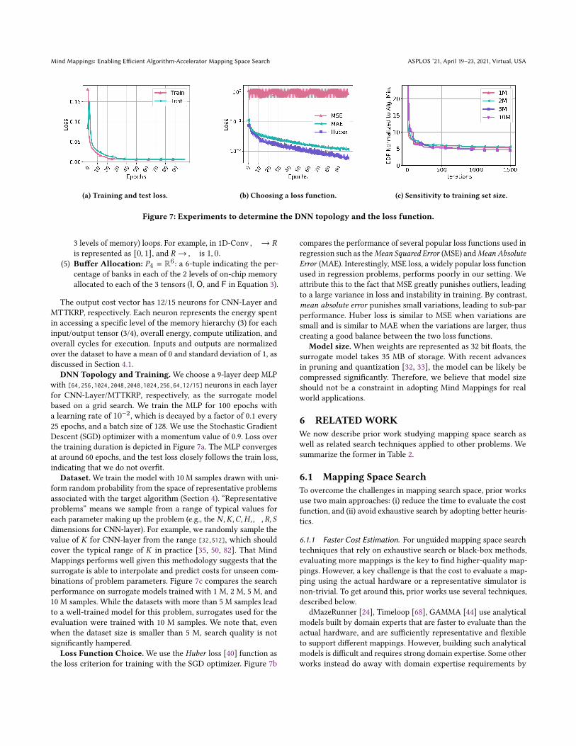
DNN Topology and Training. We choose a 9-layer deep MLPwith [64,256,1024,2048,2048,1024,256,64,12/15] neurons in each layerfor CNN-Layer/MTTKRP, respectively, as the surrogate modelbased on a grid search. We train the MLP for 100 epochs witha learning rate of 10−2, which is decayed by a factor of 0.1 every25 epochs, and a batch size of 128. We use the Stochastic GradientDescent (SGD) optimizer with a momentum value of 0.9. Loss overthe training duration is depicted in Figure 7a. The MLP convergesat around 60 epochs, and the test loss closely follows the train loss,indicating that we do not overfit.

Dataset.We train the model with 10 M samples drawn with uni-form random probability from the space of representative problemsassociated with the target algorithm (Section 4). “Representativeproblems” means we sample from a range of typical values foreach parameter making up the problem (e.g., the 𝑁,𝐾,𝐶, 𝐻,𝑊 , 𝑅, 𝑆

dimensions for CNN-layer). For example, we randomly sample thevalue of 𝐾 for CNN-layer from the range [32,512], which shouldcover the typical range of 𝐾 in practice [35, 50, 82]. That MindMappings performs well given this methodology suggests that thesurrogate is able to interpolate and predict costs for unseen com-binations of problem parameters. Figure 7c compares the searchperformance on surrogate models trained with 1 M, 2 M, 5 M, and10 M samples. While the datasets with more than 5 M samples leadto a well-trained model for this problem, surrogates used for theevaluation were trained with 10 M samples. We note that, evenwhen the dataset size is smaller than 5 M, search quality is notsignificantly hampered.

Loss Function Choice. We use the Huber loss [40] function asthe loss criterion for training with the SGD optimizer. Figure 7b

compares the performance of several popular loss functions used inregression such as theMean Squared Error (MSE) andMean AbsoluteError (MAE). Interestingly, MSE loss, a widely popular loss functionused in regression problems, performs poorly in our setting. Weattribute this to the fact that MSE greatly punishes outliers, leadingto a large variance in loss and instability in training. By contrast,mean absolute error punishes small variations, leading to sub-parperformance. Huber loss is similar to MSE when variations aresmall and is similar to MAE when the variations are larger, thuscreating a good balance between the two loss functions.

Model size.When weights are represented as 32 bit floats, thesurrogate model takes 35 MB of storage. With recent advancesin pruning and quantization [32, 33], the model can be likely becompressed significantly. Therefore, we believe that model sizeshould not be a constraint in adopting Mind Mappings for realworld applications.

6 RELATEDWORKWe now describe prior work studying mapping space search aswell as related search techniques applied to other problems. Wesummarize the former in Table 2.

6.1 Mapping Space SearchTo overcome the challenges in mapping search space, prior worksuse two main approaches: (i) reduce the time to evaluate the costfunction, and (ii) avoid exhaustive search by adopting better heuris-tics.

6.1.1 Faster Cost Estimation. For unguided mapping space searchtechniques that rely on exhaustive search or black-box methods,evaluating more mappings is the key to find higher-quality map-pings. However, a key challenge is that the cost to evaluate a map-ping using the actual hardware or a representative simulator isnon-trivial. To get around this, prior works use several techniques,described below.

dMazeRunner [24], Timeloop [68], GAMMA [44] use analyticalmodels built by domain experts that are faster to evaluate than theactual hardware, and are sufficiently representative and flexibleto support different mappings. However, building such analyticalmodels is difficult and requires strong domain expertise. Some otherworks instead do away with domain expertise requirements by


Table 2: Related works in Mapping Space Search. Mind Mappings differentiates from other works by enabling a first-orderoptimization using Gradient Descent with a differentiable surrogate.

Work Problem Domain Cost Function Search Heuristic

FlexTensor [102] Tensor Compilation Actual Hardware Reinforcement LearningTiramisu [7] DNN Compilation Actual hardware Beam SearchGamma [44] DNN Mapping Space Search Analytical Genetic Algorithm

TensorComprehensions [97] DNN Compilation Actual hardware Genetic AlgorithmsdMazeRunner [24] DNN Compilation Analytical Pruned SearchTimeloop [68] Affine loop nests Analytical Pruned SearchTVM [15] DNN Compilation Gradient Boosted Trees Simualted Annealing

RELEASE [3] DNN Compilation Gradient Boosted Trees Reinforcement LearningAdams et. al [2] Halide [76] Compilation Multi-Layer Perceptrons Beam Search

Mind Mappings (ours) Domain Agnostic Multi-Layer Perceptrons Gradient-based Search

leveraging machine learning to build an approximate cost function.For example, AutoTVM [15] and RELEASE[3] use gradient-boostedtrees [14]. On the other hand, Adams et al. [2] use Multi-layerPerceptrons (MLPs). We note that while we also use MLPs to buildthe surrogate, we utilize the differentiability of the surrogate toperform a guided search.

6.1.2 Mapping Space Search with Heuristics. Orthogonal to tech-niques mentioned in Section 6.1.1 that speed up the cost evaluation,prior works also develop custom/learnt heuristics to improve thesearch itself, so as to avoid brute-force search. dMazeRunner [24],Marvel [12] and Timeloop [68] prune the search space to reducethe number of mappings that need to be evaluated using domainexpert knowledge. The key idea is that points in the search spacecan be eliminated without evaluation, e.g., tile sizes that do not fitin the on-chip buffer. Again, this solution is difficult to scale sinceit requires extensive domain expertise to create rules to prune thesearch space.

Several prior works leverage black-box optimization methodsto perform the search. For example, AutoTVM uses parallel simu-lated annealing [45] (SA) to search through the map space. Open-Tuner [5] is a program auto-tuner that uses the AUC Bandit Metatechnique to combine several methods such as differential evolu-tion. RELEASE [3] and FlexTensor [102] both use ReinforcementLearning (RL) as the cost heuristic to guide the search. Tiramisu [7]and Adams et al [2] both employ beam search. Finally, TensorCom-prehensions [97] and GAMMA [44] use Genetic Algorithms [39],which are a popular approach used in combinatorial optimiza-tion [29, 64, 88].

For all of the above: by definition of being black box, heuristicscan only guide the search based on previously visited samples, andtherefore require a large number of samples to perform well. Asdemonstrated in Section 5, Mind Mappings outperforms SA, GA,and RL by utilizing powerful gradient-based optimization with thedifferentiable surrogate.

6.2 Related Works in other AreasBeyond mapping space search, the combinatorial search repre-sented in Equation 1 is widely found in other areas such as neuralarchitecture search [103], device placement [72], etc., and insights

from related works in these areas can apply to the mapping spacesearch problem.

Surrogate Modeling. Using surrogates for solving black-boxoptimization problems has been well explored [49]. To predict theperformance of a program on a CPU, Ithermal [62] and Difftune [78]use Recurrent Neural Networks, Ïpek et al. [42] use Artificial NeuralNets, and Lee et al. [55] use regression modeling. Deep generativemodels are proposed as a surrogate in [81], which are differentiableapproximations. Function approximation or surrogate modelinghas been at the core of modern Reinforcement Learning methodsto approximate the large state-space present in real-life problems.Similarly, Mind Mappings uses a differentiable surrogate, whilecarefully tuning the supervised training methods to adapt to themapping space search problem.

Search Heuristics. Black-box approaches such as SimulatedAnnealing, Genetic Algorithms [29, 64, 88], Bayesian Optimiza-tion [72, 77, 79], etc., have been widely used in different applications.Recent advances in Reinforcement Learning (RL) have influencedseveral works [98, 103] to adopt the same, with promising results.Several works have explored gradient-basedmethods [57, 78, 81, 99],in spite of the cost function being non-differentiable. For example,FBNet [99] uses Gumbel-Softmax [60] to make the discrete choicesin their problem differentiable, thereby obtaining gradients.

While gradient-based optimization applied to combinatorial opti-mization problems with black-box cost functions is not new [17, 31,57, 58, 78, 81, 94, 96, 99], adapting this to the mapping space searchproblem—the focus of this paper—is new and faces non-trivial chal-lenges (Section 4).

7 CONCLUSIONThis paper proposed Mind Mappings, an efficient method for per-forming algorithm-accelerator mapping space search. The key ideais to approximate the non-differentiable accelerator cost functionwith a differentiable surrogate, and to use that surrogate to performa powerful Gradient Descent-based search.

While Mind Mappings significantly closes the gap to findingoptimal mappings quickly, there is still gap left to close. In par-ticular, Section 4 details several areas where the method can befurther optimized, ranging from improved sampling methods fortraining the surrogate to more efficient encodings of accelerator


programmable attributes. Long term and with these refinements,we hope that the methods in this paper advance mapping spacesearch to a level closer to its more mature cousin, compilation forgeneral-purpose devices.

ACKNOWLEDGMENTSWe thanks the anonymous reviewers and our shepherd DanielJimenez for their valuable feedback. This work was funded in partby NSF under grant 1942888 and by DARPA SDH contract DARPASDH #HR0011-18-3-0007. Kartik Hegde was funded in part by aFacebook Ph.D. fellowship.

Appendices

A EVALUATION: POINTS OF COMPARISONWe now provide implementation details for each search methodused in Section 5.

Algorithmic Minimum. Our baseline represents the theoret-ical lower-bound EDP for the given accelerator, algorithm andproblem. We construct this oracle EDP by taking the product ofthe minimum energy and minimum execution cycles. The min-imum energy is achieved when each input data is read onlyonce and each output data is written only once at each levelin the memory hierarchy. The minimum execution cycles areachieved when PEs maintain 100% utilization, i.e., when cyclesequals 𝑟𝑒𝑞𝑢𝑖𝑟𝑒𝑑_𝑓 𝑙𝑜𝑝𝑠/(𝑓 𝑙𝑜𝑝𝑠_𝑝𝑒𝑟_𝑝𝑒 ∗ 𝑛𝑢𝑚_𝑝𝑒𝑠).

Note that in practice, one usually trades-off energy for cycles andcannot achieve the best of both worlds. Thus, the above algorithmicminimum is likely unachievable. We do not calculate the achievablelower-bound EDP, as this requires an intractable exhaustive search.

Simulated Annealing (SA).We implement SA in Python usinga popular library 𝑠𝑖𝑚𝑎𝑛𝑛𝑒𝑎𝑙 [74]. For each problem evaluation, welet the library perform auto-tuning to get the best hyper-parametersfor SA such as the temperature and annealing factor. We interfacethe library with the Mind Mappings tuner to perform mappingspace search.

Genetic Algorithm (GA). We implement GA in Python usingDEAP [28], a popular GA library. Based on the extensive literatureon parameter tuning for GA [13, 16, 34, 67, 84] and a grid search,we set an initial population size of 100 and crossover/mutationprobabilities of 0.75/0.05, respectively. Each individual is a mappingranked based on fitness, which represents the optimization objec-tive, EDP. Every iteration, we perform a cross-over and mutationover the population. A cross-over results in swapping attributesof one individual with the other while a mutation is implementedas a .05 probability of a random update for each of the mapping’sattributes. At the end of each generation, individuals are chosenbased on their fitness for the next generation.

Reinforcement Learning (RL). We implement RL in Py-Torch [71], based on the Deep Deterministic Policy Gradient(DDPG) [56] implementation from HAQ [98]. In the RL setting,the mapping problem is modeled as a Markov Decision Process(MDP) [8], where each mapping is a state in the MDP, an actionresults in a move to a target state and the cost of the mapping is thereward. In each episode, the RL agent starts from a random initial

state, takes an action to move to a target state and updates its policybased on the reward. In this process, the agent learns the optimalaction to take given a state in the space. The learning process usesthe actor-critic method [48], which is a widely-used policy gradientalgorithm. The actor and critic functions are approximated withtwo fully-connected DNNs with 300 neurons respectively.

Mind Mappings (MM). We implement Mind Mappings (Sec-tion 4) using a trained surrogate model (elaborated in Section 4.2) asdescribed in Section 4.1. We inject randomness at an interval of ev-ery 10 iterations to avoid local minimas, as described in Section 4.2.We use simulated annealing with a temperature of 50 initially to de-cide the acceptance of random injections, which is annealed every50 injections by a factor of 0.75. We use a learning rate of 1, andwe do not decay the learning rate throughout the procedure. Wechoose the learning rates and injection interval via a grid search.

B MIND MAPPINGS APIThe Mind Mappings API exposes an optimization framework formapping space search that can be used in compilers and frameworkstargeting a specialized hardware accelerator, such as TVM [15],PyTorch [71], TensorFlow [1], etc. A surrogate model is trainedoffline for the target algorithm-accelerator pair to approximatemapping cost, using techniques described in Section 4.1. Then,during the compilation, the Mind Mappings API takes the trainedsurrogatemodel and the target problem 𝑝 as input and returns a low-cost (ideally optimal) mapping𝑚𝑜𝑝𝑡 that minimizes the problem’sexecution cost on the given accelerator.

The Mind Mappings API requires the following routines: (1)getMapping: gives a random valid mapping, (2) isMember: checksif a mapping is valid, and (3) getProjection: returns a projectionfrom an invalid mapping to the nearest valid mapping. We haveopen sourced the Mind Mappings framework here: https://github.com/kartik-hegde/mindMappings.

REFERENCES[1] Martín Abadi, Ashish Agarwal, Paul Barham, Eugene Brevdo, Zhifeng Chen,

Craig Citro, Greg S. Corrado, Andy Davis, Jeffrey Dean, Matthieu Devin, San-jay Ghemawat, Ian Goodfellow, Andrew Harp, Geoffrey Irving, Michael Isard,Yangqing Jia, Rafal Jozefowicz, Lukasz Kaiser, Manjunath Kudlur, Josh Lev-enberg, Dandelion Mané, Rajat Monga, Sherry Moore, Derek Murray, ChrisOlah, Mike Schuster, Jonathon Shlens, Benoit Steiner, Ilya Sutskever, KunalTalwar, Paul Tucker, Vincent Vanhoucke, Vijay Vasudevan, Fernanda Viégas,Oriol Vinyals, Pete Warden, Martin Wattenberg, Martin Wicke, Yuan Yu, andXiaoqiang Zheng. 2015. TensorFlow: Large-Scale Machine Learning on Het-erogeneous Systems. https://www.tensorflow.org/ Software available fromtensorflow.org.

[2] Andrew Adams, Karima Ma, Luke Anderson, Riyadh Baghdadi, Tzu-Mao Li,Michaël Gharbi, Benoit Steiner, Steven Johnson, Kayvon Fatahalian, Frédo Du-rand, et al. 2019. Learning to optimize halide with tree search and randomprograms. ACM Transactions on Graphics (TOG) 38, 4 (2019), 1–12.

[3] Byung Hoon Ahn, Prannoy Pilligundla, and Hadi Esmaeilzadeh. 2019. Rein-forcement Learning and Adaptive Sampling for Optimized DNN Compilation.arXiv preprint arXiv:1905.12799 (2019).

[4] Jorge Albericio, Patrick Judd, Tayler Hetherington, Tor Aamodt, Natalie EnrightJerger, and Andreas Moshovos. 2016. Cnvlutin: ineffectual-neuron-free deepneural network computing. In Proceedings of the 43rd International Symposiumon Computer Architecture. 1–13.

[5] Jason Ansel, Shoaib Kamil, Kalyan Veeramachaneni, Jonathan Ragan-Kelley,Jeffrey Bosboom, Una-May O’Reilly, and Saman Amarasinghe. 2014. OpenTuner:An Extensible Framework for Program Autotuning. In International Conferenceon Parallel Architectures and Compilation Techniques. Edmonton, Canada. http://groups.csail.mit.edu/commit/papers/2014/ansel-pact14-opentuner.pdf

[6] Charles Audet, J Denni, Douglas Moore, Andrew Booker, and Paul Frank. 2000. Asurrogate-model-based method for constrained optimization. In 8th symposium

https://github.com/kartik-hegde/mindMappings

https://github.com/kartik-hegde/mindMappings

https://www.tensorflow.org/

http://groups.csail.mit.edu/commit/papers/2014/ansel-pact14-opentuner.pdf

http://groups.csail.mit.edu/commit/papers/2014/ansel-pact14-opentuner.pdf


on multidisciplinary analysis and optimization.[7] Riyadh Baghdadi, Jessica Ray, Malek Ben Romdhane, Emanuele Del Sozzo,

Abdurrahman Akkas, Yunming Zhang, Patricia Suriana, Shoaib Kamil, andSaman Amarasinghe. 2019. Tiramisu: A polyhedral compiler for expressing fastand portable code. In Proceedings of the 2019 IEEE/ACM International Symposiumon Code Generation and Optimization. IEEE Press, 193–205.

[8] Richard Bellman. 1957. A Markovian decision process. Journal of mathematicsand mechanics (1957), 679–684.

[9] Eliot Bolduc, George CKnee, ErikMGauger, and Jonathan Leach. 2017. Projectedgradient descent algorithms for quantum state tomography. npj QuantumInformation 3, 1 (2017), 1–9.

[10] Justin A Boyan and Andrew W Moore. 1995. Generalization in reinforcementlearning: Safely approximating the value function. In Advances in neural infor-mation processing systems. 369–376.

[11] J Douglas Carroll and Jih-Jie Chang. 1970. Analysis of individual differencesin multidimensional scaling via an N-way generalization of “Eckart-Young”decomposition. Psychometrika 35, 3 (1970), 283–319.

[12] Prasanth Chatarasi, Hyoukjun Kwon, Natesh Raina, Saurabh Malik, VaisakhHaridas, Tushar Krishna, and Vivek Sarkar. 2020. MARVEL: A DecoupledModel-driven Approach for Efficiently Mapping Convolutions on Spatial DNNAccelerators. arXiv preprint arXiv:2002.07752 (2020).

[13] Stephen Chen, James Montgomery, and Antonio Bolufé-Röhler. 2015. Measuringthe curse of dimensionality and its effects on particle swarm optimization anddifferential evolution. Applied Intelligence 42, 3 (2015), 514–526.

[14] Tianqi Chen and Carlos Guestrin. 2016. Xgboost: A scalable tree boosting system.In Proceedings of the 22nd acm sigkdd international conference on knowledgediscovery and data mining. ACM, 785–794.

[15] Tianqi Chen, Thierry Moreau, Ziheng Jiang, Lianmin Zheng, Eddie Yan, HaichenShen, Meghan Cowan, LeyuanWang, Yuwei Hu, Luis Ceze, et al. 2018. TVM: Anautomated end-to-end optimizing compiler for deep learning. In 13th USENIXSymposium on Operating Systems Design and Implementation (OSDI 18). 578–594.

[16] Tianshi Chen, Ke Tang, Guoliang Chen, and Xin Yao. 2012. A large populationsize can be unhelpful in evolutionary algorithms. Theoretical Computer Science436 (2012), 54–70.

[17] Wenzheng Chen, Parsa Mirdehghan, Sanja Fidler, and Kiriakos N Kutulakos.2020. Auto-Tuning Structured Light by Optical Stochastic Gradient Descent. InProceedings of the IEEE/CVF Conference on Computer Vision and Pattern Recogni-tion.

[18] Yunji Chen, Tao Luo, Shaoli Liu, Shijin Zhang, Liqiang He, Jia Wang, Ling Li,Tianshi Chen, Zhiwei Xu, Ninghui Sun, et al. 2014. Dadiannao: A machine-learning supercomputer. In 2014 47th Annual IEEE/ACM International Symposiumon Microarchitecture. IEEE, 609–622.

[19] Yudong Chen and Martin J Wainwright. 2015. Fast low-rank estimation byprojected gradient descent: General statistical and algorithmic guarantees. arXivpreprint arXiv:1509.03025 (2015).

[20] Yu-Hsin Chen, Joel Emer, and Vivienne Sze. 2016. Eyeriss: A Spatial Archi-tecture for Energy-Efficient Dataflow for Convolutional Neural Networks. In2016 ACM/IEEE 43rd Annual International Symposium on Computer Architecture(ISCA). IEEE, 367–379.

[21] Yu-Hsin Chen, Tien-Ju Yang, Joel Emer, and Vivienne Sze. 2019. Eyeriss v2:A flexible accelerator for emerging deep neural networks on mobile devices.IEEE Journal on Emerging and Selected Topics in Circuits and Systems 9, 2 (2019),292–308.

[22] Jason Chiang, Michael Studniberg, Jack Shaw, Stephen Seto, and Kevin Truong.2006. Hardware accelerator for genomic sequence alignment. In 2006 Interna-tional Conference of the IEEE Engineering in Medicine and Biology Society. IEEE,5787–5789.

[23] Jason Chiang, Michael Studniberg, Jack Shaw, Stephen Seto, and Kevin Truong.2006. Hardware accelerator for genomic sequence alignment. In 2006 Interna-tional Conference of the IEEE Engineering in Medicine and Biology Society. IEEE,5787–5789.

[24] Shail Dave, Youngbin Kim, Sasikanth Avancha, Kyoungwoo Lee, and AviralShrivastava. 2019. DMazerunner: Executing perfectly nested loops on dataflowaccelerators. ACM Transactions on Embedded Computing Systems (TECS) 18, 5s(2019), 1–27.

[25] Jia Deng, Wei Dong, Richard Socher, Li-Jia Li, Kai Li, and Li Fei-Fei. 2009.Imagenet: A large-scale hierarchical image database. In 2009 IEEE conference oncomputer vision and pattern recognition. Ieee, 248–255.

[26] Zidong Du, Robert Fasthuber, Tianshi Chen, Paolo Ienne, Ling Li, Tao Luo,Xiaobing Feng, Yunji Chen, and Olivier Temam. 2015. ShiDianNao: Shiftingvision processing closer to the sensor. In ACM SIGARCH Computer ArchitectureNews, Vol. 43. ACM, 92–104.

[27] Hans Eberle, Nils Gura, Daniel Finchelstein, Sheueling Chang-Shantz, and VipulGupta. 2009. Hardware accelerator for elliptic curve cryptography. US Patent7,508,936.

[28] Félix-Antoine Fortin, François-Michel De Rainville, Marc-André Gardner, MarcParizeau, and Christian Gagné. 2012. DEAP: Evolutionary Algorithms MadeEasy. Journal of Machine Learning Research 13 (july 2012), 2171–2175.

[29] David E Goldberg. 2006. Genetic algorithms. Pearson Education India.[30] Daniel Golovin, Benjamin Solnik, Subhodeep Moitra, Greg Kochanski, John

Karro, and D Sculley. 2017. Google vizier: A service for black-box optimization.In Proceedings of the 23rd ACM SIGKDD International Conference on KnowledgeDiscovery and Data Mining. ACM, 1487–1495.

[31] Will Grathwohl, Dami Choi, Yuhuai Wu, Geoffrey Roeder, and David Duvenaud.2017. Backpropagation through the void: Optimizing control variates for black-box gradient estimation. arXiv preprint arXiv:1711.00123 (2017).

[32] Song Han, Xingyu Liu, Huizi Mao, Jing Pu, Ardavan Pedram, Mark A Horowitz,and William J Dally. 2016. EIE: Efficient Inference Engine on Compressed DeepNeural Network. In 2016 ACM/IEEE 43rd Annual International Symposium onComputer Architecture (ISCA). IEEE Computer Society, 243–254.

[33] Song Han, Huizi Mao, and William J Dally. 2015. Deep compression: Com-pressing deep neural networks with pruning, trained quantization and huffmancoding. arXiv preprint arXiv:1510.00149 (2015).

[34] Ahmad Hassanat, Khalid Almohammadi, Esra’ Alkafaween, Eman Abunawas,Awni Hammouri, and VB Prasath. 2019. Choosing Mutation and CrossoverRatios for Genetic Algorithms—A Review with a New Dynamic Approach.Information 10, 12 (2019), 390.

[35] Kaiming He, Xiangyu Zhang, Shaoqing Ren, and Jian Sun. 2016. Deep residuallearning for image recognition. In Proceedings of the IEEE conference on computervision and pattern recognition. 770–778.

[36] Kartik Hegde, Rohit Agrawal, Yulun Yao, and Christopher W Fletcher. 2018.Morph: Flexible Acceleration for 3D CNN-based Video Understanding. In 201851st Annual IEEE/ACM International Symposium on Microarchitecture (MICRO).IEEE, 933–946.

[37] Kartik Hegde, Hadi Asghari-Moghaddam, Michael Pellauer, Neal Crago, AamerJaleel, Edgar Solomonik, Joel Emer, and Christopher W Fletcher. 2019. ExTensor:An Accelerator for Sparse Tensor Algebra. In Proceedings of the 52nd AnnualIEEE/ACM International Symposium on Microarchitecture. 319–333.

[38] Kartik Hegde, Jiyong Yu, Rohit Agrawal, Mengjia Yan, Michael Pellauer, andChristopher Fletcher. 2018. Ucnn: Exploiting computational reuse in deep neuralnetworks via weight repetition. In 2018 ACM/IEEE 45th Annual InternationalSymposium on Computer Architecture (ISCA). IEEE, 674–687.

[39] JohnHenry Holland et al. 1992. Adaptation in natural and artificial systems: an in-troductory analysis with applications to biology, control, and artificial intelligence.MIT press.

[40] Peter J Huber. 1992. Robust estimation of a location parameter. In Breakthroughsin statistics. Springer, 492–518.

[41] Tassadaq Hussain, Oscar Palomar, Adrian Cristal, Eduard Ayguadé, and AmnaHaider. 2015. ViPS: Visual processing system for medical imaging. In 2015 8thInternational Conference on Biomedical Engineering and Informatics (BMEI). IEEE,40–45.

[42] Engin Ïpek, Sally A McKee, Rich Caruana, Bronis R de Supinski, and MartinSchulz. 2006. Efficiently exploring architectural design spaces via predictivemodeling. ACM SIGOPS Operating Systems Review 40, 5 (2006), 195–206.

[43] Norman P Jouppi, Cliff Young, Nishant Patil, David Patterson, Gaurav Agrawal,Raminder Bajwa, Sarah Bates, Suresh Bhatia, Nan Boden, Al Borchers, et al. 2017.In-datacenter performance analysis of a tensor processing unit. In Proceedingsof the 44th annual international symposium on computer architecture. 1–12.

[44] Sheng-Chun Kao and Tushar Krishna. 2020. GAMMA: automating the HWmap-ping of DNN models on accelerators via genetic algorithm. In 2020 IEEE/ACMInternational Conference On Computer Aided Design (ICCAD). IEEE.

[45] Scott Kirkpatrick, C Daniel Gelatt, and Mario P Vecchi. 1983. Optimization bysimulated annealing. science 220, 4598 (1983), 671–680.

[46] Robert Kleinberg, Yuanzhi Li, and Yang Yuan. 2018. An alternative view: Whendoes SGD escape local minima? arXiv preprint arXiv:1802.06175 (2018).

[47] Tamara G Kolda and Brett W Bader. 2009. Tensor decompositions and applica-tions. SIAM review 51, 3 (2009), 455–500.

[48] Vijay R Konda and John N Tsitsiklis. 2000. Actor-critic algorithms. In Advancesin neural information processing systems. 1008–1014.

[49] Slawomir Koziel and Leifur Leifsson. 2013. Surrogate-based modeling and opti-mization. Springer.

[50] Alex Krizhevsky, Ilya Sutskever, and Geoffrey E Hinton. 2012. Imagenet classifi-cation with deep convolutional neural networks. Advances in neural informationprocessing systems 25 (2012), 1097–1105.

[51] Hyoukjun Kwon, Prasanth Chatarasi, Michael Pellauer, Angshuman Parashar,Vivek Sarkar, and Tushar Krishna. 2019. Understanding Reuse, Performance,and Hardware Cost of DNN Dataflow: A Data-Centric Approach. In Proceedingsof the 52nd Annual IEEE/ACM International Symposium on Microarchitecture.ACM, 754–768.

[52] Hyoukjun Kwon, Ananda Samajdar, and Tushar Krishna. 2018. MAERI: En-abling Flexible Dataflow Mapping over DNN Accelerators via ReconfigurableInterconnects. SIGPLAN Not. 53, 2 (March 2018), 461–475. https://doi.org/10.1145/3296957.3173176

[53] Yann LeCun, D Touresky, G Hinton, and T Sejnowski. 1988. A theoreticalframework for back-propagation. In Proceedings of the 1988 connectionist modelssummer school, Vol. 1. CMU, Pittsburgh, Pa: Morgan Kaufmann, 21–28.

https://doi.org/10.1145/3296957.3173176

https://doi.org/10.1145/3296957.3173176


[54] Yann A. LeCun, Léon Bottou, Genevieve B. Orr, and Klaus-Robert Müller. 2012.Efficient BackProp. Springer Berlin Heidelberg, Berlin, Heidelberg, 9–48. https://doi.org/10.1007/978-3-642-35289-8_3

[55] Benjamin C Lee and David M Brooks. 2007. Illustrative design space studies withmicroarchitectural regression models. In 2007 IEEE 13th International Symposiumon High Performance Computer Architecture. IEEE, 340–351.

[56] Timothy P. Lillicrap, Jonathan J. Hunt, Alexander Pritzel, Nicolas Heess, TomErez, Yuval Tassa, David Silver, and Daan Wierstra. 2016. Continuous controlwith deep reinforcement learning. In 4th International Conference on LearningRepresentations, ICLR 2016, San Juan, Puerto Rico, May 2-4, 2016, ConferenceTrack Proceedings. http://arxiv.org/abs/1509.02971

[57] Hanxiao Liu, Karen Simonyan, and Yiming Yang. 2018. Darts: Differentiablearchitecture search. arXiv preprint arXiv:1806.09055 (2018).

[58] Gilles Louppe, Joeri Hermans, and Kyle Cranmer. 2017. Adversarial variationaloptimization of non-differentiable simulators. arXiv preprint arXiv:1707.07113(2017).

[59] Wenyan Lu, Guihai Yan, Jiajun Li, Shijun Gong, Yinhe Han, and Xiaowei Li.2017. Flexflow: A flexible dataflow accelerator architecture for convolutionalneural networks. In 2017 IEEE International Symposium on High PerformanceComputer Architecture (HPCA). IEEE, 553–564.

[60] Chris J Maddison, Andriy Mnih, and Yee Whye Teh. 2016. The concrete distri-bution: A continuous relaxation of discrete random variables. arXiv preprintarXiv:1611.00712 (2016).

[61] Sanu Mathew, Sudhir Satpathy, Vikram Suresh, Mark Anders, Himanshu Kaul,Amit Agarwal, Steven Hsu, Gregory Chen, and Ram Krishnamurthy. 2015. 340mV–1.1 V, 289 Gbps/W, 2090-gate nanoAES hardware accelerator with area-optimized encrypt/decrypt GF (2 4) 2 polynomials in 22 nm tri-gate CMOS. IEEEJournal of Solid-State Circuits 50, 4 (2015), 1048–1058.

[62] Charith Mendis, Alex Renda, Saman Amarasinghe, and Michael Carbin. 2018.Ithemal: Accurate, portable and fast basic block throughput estimation usingdeep neural networks. arXiv preprint arXiv:1808.07412 (2018).

[63] Tomas Mikolov, Kai Chen, Gregory S. Corrado, and Jeffrey Dean. 2013. EfficientEstimation ofWord Representations in Vector Space. CoRR abs/1301.3781 (2013).

[64] AnjumAMohammed andGihanNagib. 2012. Optimal routing in ad-hoc networkusing genetic algorithm. Int. J. Advanced Networking and Applications 3, 05(2012), 1323–1328.

[65] Yurii Nesterov. 2013. Introductory lectures on convex optimization: A basic course.Vol. 87. Springer Science & Business Media.

[66] NVIDIA. [n.d.]. The NVIDIA Deep Learning Accelerator (NVDLA). http://nvdla.org/hw/v1/ias/programming_guide.html.

[67] Hari Mohan Pandey, Ankit Chaudhary, and Deepti Mehrotra. 2014. A compara-tive review of approaches to prevent premature convergence in GA. AppliedSoft Computing 24 (2014), 1047–1077.

[68] Angshuman Parashar, Priyanka Raina, Yakun Sophia Shao, Yu-Hsin Chen,Victor A Ying, Anurag Mukkara, Rangharajan Venkatesan, Brucek Khailany,Stephen W Keckler, and Joel Emer. 2019. Timeloop: A Systematic Approach toDNN Accelerator Evaluation. In 2019 IEEE International Symposium on Perfor-mance Analysis of Systems and Software (ISPASS). IEEE, 304–315.

[69] Angshuman Parashar, Minsoo Rhu, Anurag Mukkara, Antonio Puglielli, Rang-harajan Venkatesan, Brucek Khailany, Joel Emer, Stephen W Keckler, andWilliam J Dally. 2017. SCNN: An accelerator for compressed-sparse convolu-tional neural networks. In 2017 ACM/IEEE 44th Annual International Symposiumon Computer Architecture (ISCA). IEEE, 27–40.

[70] Razvan Pascanu, Tomas Mikolov, and Yoshua Bengio. 2012. Understanding theexploding gradient problem. CoRR, abs/1211.5063 2 (2012).

[71] Adam Paszke, Sam Gross, Francisco Massa, Adam Lerer, James Bradbury, Gre-gory Chanan, Trevor Killeen, Zeming Lin, Natalia Gimelshein, Luca Antiga, et al.2019. PyTorch: An imperative style, high-performance deep learning library. InAdvances in Neural Information Processing Systems. 8024–8035.

[72] Tirthak Patel and Devesh Tiwari. 2020. CLITE: Efficient and QoS-Aware Co-Location of Multiple Latency-Critical Jobs for Warehouse Scale Computers. In2020 IEEE International Symposium on High Performance Computer Architecture(HPCA). IEEE, 193–206.

[73] Michael Pellauer, Yakun Sophia Shao, Jason Clemons, Neal Crago, Kartik Hegde,Rangharajan Venkatesan, Stephen W Keckler, Christopher W Fletcher, and JoelEmer. 2019. Buffets: An efficient and composable storage idiom for explicitdecoupled data orchestration. In Proceedings of the Twenty-Fourth InternationalConference on Architectural Support for Programming Languages and OperatingSystems. 137–151.

[74] Matthew Perry. 2019. Python module for simulated annealing. https://github.com/perrygeo/simanneal.

[75] Nestor V Queipo, Raphael T Haftka, Wei Shyy, Tushar Goel, RajkumarVaidyanathan, and P Kevin Tucker. 2005. Surrogate-based analysis and op-timization. Progress in aerospace sciences (2005).

[76] Jonathan Ragan-Kelley, Connelly Barnes, Andrew Adams, Sylvain Paris, FrédoDurand, and Saman Amarasinghe. 2013. Halide: a language and compilerfor optimizing parallelism, locality, and recomputation in image processingpipelines. In Acm Sigplan Notices, Vol. 48. ACM, 519–530.

[77] Brandon Reagen, José Miguel Hernández-Lobato, Robert Adolf, Michael Gelbart,Paul Whatmough, Gu-Yeon Wei, and David Brooks. 2017. A case for efficient ac-celerator design space exploration via Bayesian optimization. In 2017 IEEE/ACMInternational Symposium on Low Power Electronics and Design (ISLPED). IEEE,1–6.

[78] Alex Renda, Yishen Chen, Charith Mendis, and Michael Carbin. 2020. DiffTune:Optimizing CPU Simulator Parameters with Learned Differentiable Surrogates.In 2020 53rd Annual IEEE/ACM International Symposium on Microarchitecture(MICRO). IEEE.

[79] Raanan Y Rohekar, Shami Nisimov, Yaniv Gurwicz, Guy Koren, and Gal Novik.2018. Constructing deep neural networks by Bayesian network structure learn-ing. In Advances in Neural Information Processing Systems. 3047–3058.

[80] Ananda Samajdar, Yuhao Zhu, Paul Whatmough, Matthew Mattina, andTushar Krishna. 2018. Scale-sim: Systolic cnn accelerator. arXiv preprintarXiv:1811.02883 (2018).

[81] Sergey Shirobokov, Vladislav Belavin, Michael Kagan, Andrei Ustyuzhanin,and Atilim Gunes Baydin. 2020. Black-box optimization with local generativesurrogates. InWorkshop on Real World Experiment Design and Active Learningat International Conference on Machine Learning.

[82] Karen Simonyan and Andrew Zisserman. 2014. Very Deep ConvolutionalNetworks for Large-Scale Image Recognition. CoRR abs/1409.1556 (2014). http://arxiv.org/abs/1409.1556

[83] Age Smilde, Rasmus Bro, and Paul Geladi. 2005. Multi-way analysis: applicationsin the chemical sciences. John Wiley & Sons.

[84] Selmar K Smit and AE Eiben. 2010. Parameter tuning of evolutionary algo-rithms: Generalist vs. specialist. In European conference on the applications ofevolutionary computation. Springer, 542–551.

[85] Shaden Smith, Jongsoo Park, and George Karypis. 2017. Sparse tensor fac-torization on many-core processors with high-bandwidth memory. In 2017IEEE International Parallel and Distributed Processing Symposium (IPDPS). IEEE,1058–1067.

[86] Nitish Srivastava, Geoffrey Hinton, Alex Krizhevsky, Ilya Sutskever, and RuslanSalakhutdinov. 2014. Dropout: a simple way to prevent neural networks fromoverfitting. The journal of machine learning research 15, 1 (2014), 1929–1958.

[87] Nitish Srivastava, Hanchen Jin, Shaden Smith, Hongbo Rong, David Albonesi,and Zhiru Zhang. 2020. Tensaurus: A versatile accelerator for mixed sparse-dense tensor computations. In 2020 IEEE International Symposium on HighPerformance Computer Architecture (HPCA). IEEE, 689–702.

[88] Praveen Ranjan Srivastava and Tai-hoon Kim. 2009. Application of geneticalgorithm in software testing. International Journal of software Engineering andits Applications 3, 4 (2009), 87–96.

[89] Rainer Storn and Kenneth Price. 1997. Differential evolution–a simple andefficient heuristic for global optimization over continuous spaces. Journal ofglobal optimization 11, 4 (1997), 341–359.

[90] Richard S Sutton, David A McAllester, Satinder P Singh, and Yishay Mansour.2000. Policy gradient methods for reinforcement learning with function approx-imation. In Advances in neural information processing systems. 1057–1063.

[91] Richard S Sutton, David A McAllester, Satinder P Singh, Yishay Mansour, et al.1999. Policy gradient methods for reinforcement learning with function approx-imation.. In NIPs, Vol. 99. Citeseer, 1057–1063.

[92] Christian Szegedy, Wei Liu, Yangqing Jia, Pierre Sermanet, Scott Reed, DragomirAnguelov, Dumitru Erhan, Vincent Vanhoucke, and Andrew Rabinovich. 2015.Going deeper with convolutions. In Proceedings of the IEEE conference on com-puter vision and pattern recognition. 1–9.

[93] G Tomasi. 2005. Use of the properties of the Khatri-Rao product for the compu-tation of Jacobian. Hessian, and gradient of the PARAFAC model under MATLAB(2005).

[94] Ethan Tseng, Felix Yu, Yuting Yang, Fahim Mannan, Karl ST Arnaud, DerekNowrouzezahrai, Jean-François Lalonde, and Felix Heide. 2019. Hyperparameteroptimization in black-box image processing using differentiable proxies. ACMTransactions on Graphics (2019).

[95] Fengbin Tu, Shouyi Yin, Peng Ouyang, Shibin Tang, Leibo Liu, and ShaojunWei. 2017. Deep convolutional neural network architecture with reconfigurablecomputation patterns. IEEE Transactions on Very Large Scale Integration (VLSI)Systems 25, 8 (2017), 2220–2233.

[96] George Tucker, Andriy Mnih, Chris J Maddison, Dieterich Lawson, and JaschaSohl-Dickstein. 2017. Rebar: Low-variance, unbiased gradient estimates fordiscrete latent variable models. arXiv preprint arXiv:1703.07370 (2017).

[97] Nicolas Vasilache, Oleksandr Zinenko, Theodoros Theodoridis, Priya Goyal,Zachary DeVito,William SMoses, Sven Verdoolaege, AndrewAdams, and AlbertCohen. 2018. Tensor comprehensions: Framework-agnostic high-performancemachine learning abstractions. arXiv preprint arXiv:1802.04730 (2018).

[98] Kuan Wang, Zhijian Liu, Yujun Lin, Ji Lin, and Song Han. 2019. Haq: Hardware-aware automated quantization with mixed precision. In Proceedings of the IEEEconference on computer vision and pattern recognition. 8612–8620.

[99] Bichen Wu, Xiaoliang Dai, Peizhao Zhang, Yanghan Wang, Fei Sun, YimingWu, Yuandong Tian, Peter Vajda, Yangqing Jia, and Kurt Keutzer. 2019. Fbnet:Hardware-aware efficient convnet design via differentiable neural architecture

https://doi.org/10.1007/978-3-642-35289-8_3

https://doi.org/10.1007/978-3-642-35289-8_3

http://arxiv.org/abs/1509.02971

http://nvdla.org/hw/v1/ias/programming_guide.html

http://nvdla.org/hw/v1/ias/programming_guide.html

https://github.com/perrygeo/simanneal

https://github.com/perrygeo/simanneal




search. In Proceedings of the IEEE Conference on Computer Vision and PatternRecognition. 10734–10742.

[100] Amir Yazdanbakhsh, Kambiz Samadi, Nam Sung Kim, and Hadi Esmaeilzadeh.2018. Ganax: A unified mimd-simd acceleration for generative adversarialnetworks. In 2018 ACM/IEEE 45th Annual International Symposium on ComputerArchitecture (ISCA). IEEE, 650–661.

[101] Jiecao Yu, Andrew Lukefahr, David Palframan, Ganesh Dasika, Reetuparna Das,and Scott Mahlke. 2017. Scalpel: Customizing DNN Pruning to the UnderlyingHardware Parallelism. In Proceedings of the 44th Annual International Symposium

on Computer Architecture. 548–560.[102] Size Zheng, Yun Liang, Shuo Wang, Renze Chen, and Kaiwen Sheng. 2020. Flex-

Tensor: An Automatic Schedule Exploration and Optimization Framework forTensor Computation on Heterogeneous System. In Proceedings of the Twenty-Fifth International Conference on Architectural Support for Programming Lan-guages and Operating Systems. 859–873.

[103] Barret Zoph and Quoc V Le. 2016. Neural architecture search with reinforcementlearning. arXiv preprint arXiv:1611.01578 (2016).

Documents

Mind Mappings: Enabling Efficient Algorithm-Accelerator