Minimizing errors in sub-regional scale wave modeling · Minimizing errors in sub-regional scale wave modeling: Design of a forecasting system for the Nearshore Canyon Experiment

Minimizing errors in subMinimizing errors in sub--regional scale regional scale wave modeling:wave modeling:

Design of a forecasting system for the Nearshore Canyon Design of a forecasting system for the Nearshore Canyon ExperimentExperiment

Presented byPresented by: : Erick Rogers (Naval Research Laboratory, Stennis Space Center, MErick Rogers (Naval Research Laboratory, Stennis Space Center, MS)S)

CoCo--authorsauthors::James Kaihatu, Larry Hsu, David Wang, James Dykes (NRLJames Kaihatu, Larry Hsu, David Wang, James Dykes (NRL--Stennis)Stennis)

Robert Jensen (ERDC, Vicksburg, MS)Robert Jensen (ERDC, Vicksburg, MS)

8th International Workshop on Wave Hindcasting and Forecasting8th International Workshop on Wave Hindcasting and Forecasting

Nov. 14Nov. 14--19, 200419, 2004

[a [a pdfpdf of this paper is available, also some hard copies]of this paper is available, also some hard copies]

Nearshore Canyon Experiment Nearshore Canyon Experiment (NCEX) (Sponsor: ONR)(NCEX) (Sponsor: ONR)

• Large, multi-investigator experiment located at Scripps Institution of Oceanography (CA), Sept.-Dec. 2003

• Primary locations of instrumentation: Black’s Beach and Torrey Pines Beach

• Complex canyon bathymetry leads to severe wave refraction effects

Graphic courtesy of Dr. Michele Okihiro, SIO

NRL’s Wave Forecasting System for Nearshore Canyon Experiment (NCEX) (Sponsor: ONR)

In support of the Nearshore Canyon Experiment (NCEX)…•to help plan instrument deployment, •gauge the arrival of interesting wave conditions, and•anticipate the arrival of heavy surfer traffic to Black’s Beach, the primary site of instrumentation for the experiment.

http://www7320.nrlssc.navy.mil/NCEX/NCEX_mod.htm

(Graphics from http://science.whoi.edu/users/elgar/NCEX/ncex.html)

Also: •Test-bed for realtime modeling with SWAN at sub-regional scale•Wealth of data all over the SOCAL Bight

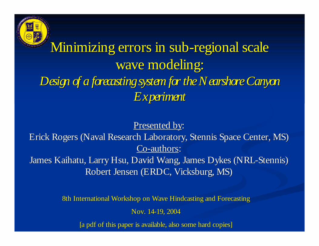
Pre-existing sub-regional Navy operational product: NAVO Southern California Bight WAM (too coarse?)

NCEX

Wave Forecasting System for Nearshore Canyon Experiment (NCEX) (Sponsor: ONR)

SWAN Outer Nest Forced by Wavewatch III

Second Level SWAN Nest

Finest SWAN Nest over NCEX Domain

Forecast Time Series at Pt. La Jolla

Real-time comparison to data


Wave Forecasting System for Nearshore Canyon Experiment (NCEX) (Sponsor:

ONR)

1st (outermost) SWAN Nest

•Boundary forcing from Wavewatch III : input spectra uniform along each boundary, from NCEP ENP wave model•Geographic resolution: 1.67 ′ (lat) × 2.0′ (lon)•Wind forcing from NCEP global model•Computation Mode: Nonstationary

•Time-lagging of swells is correctly represented•Expensive: (so run on 8 threads on 1.3 GHz IBM-P4 at NAVO MSRC using new OpenMP SWAN)

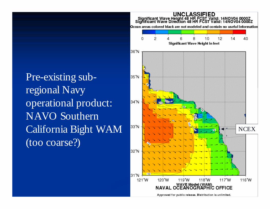
21 locations in all, wave height, peak period (and mean direction where available)ftp://ftp7300.nrlssc.navy.mil/pub/rogers/NCEX/validationSee error statistics (for wave height) in the paper.

Validation of Realtime System after NCEX ended

Buoy Wave Height (m)

Mod

el W

ave

Hei

ght (

m)

H (m

)Tp

(m)

Location: Scripps Pier

Location: Scripps Pier

Time

Minimizing ErrorsMinimizing Errors

nn …but getting the job done within operational …but getting the job done within operational time constraintstime constraints

nn What shortcuts are ok? What are not?What shortcuts are ok? What are not?nn Not a question of tuningNot a question of tuningnn Source/sink terms of wave generation secondarySource/sink terms of wave generation secondary

nn Accuracy of wind forcing also secondaryAccuracy of wind forcing also secondarynn Propagation is keyPropagation is key

Idealized CasesIdealized Cases

nn Objective: Estimate penalty from two Objective: Estimate penalty from two computational “shortcuts”:computational “shortcuts”:nn Stationary computationsStationary computationsnn Coarse geographic resolution (e.g. of islands, shoals)Coarse geographic resolution (e.g. of islands, shoals)

nn Strategy: Simple cases + Measured time series of Strategy: Simple cases + Measured time series of wind/wave conditions wind/wave conditions

Hindcasts descriptionHindcasts description

nn Four hindcasts. Only the outer SWAN Grid Four hindcasts. Only the outer SWAN Grid (SC1) is varied:(SC1) is varied:

1.1. SC1 at high resolutionSC1 at high resolution11 and computed in nonstationary mode.and computed in nonstationary mode.2.2. SC1 at high resolution and computed in stationary mode. SC1 at high resolution and computed in stationary mode. 3.3. SC1 at low resolutionSC1 at low resolution22 and computed in nonstationary mode.and computed in nonstationary mode.4.4. SC1 at low resolution and computed in stationary mode.SC1 at low resolution and computed in stationary mode.

nn This allows us to study the practical effect of two This allows us to study the practical effect of two computational “short cuts” computational “short cuts”

1.1. Using coarse resolution to describe propagation near island Using coarse resolution to describe propagation near island groupsgroups

2.2. Using the stationary assumption for a regional scale modelUsing the stationary assumption for a regional scale model

11: ∆x=∆y=1′2: ∆x=∆y=3′

Hindcasts descriptionHindcasts description

nn 3 nested SWAN grids, as with realtime model3 nested SWAN grids, as with realtime modelnn Boundary forcing of outer grid:Boundary forcing of outer grid:

nn CDIP spectra along west boundary (assumed uniform)CDIP spectra along west boundary (assumed uniform)nn NCEP WW3 spectra along south boundary (assumed uniform, NCEP WW3 spectra along south boundary (assumed uniform,

since only available at one point)since only available at one point)

nn Wind forcing: NWS global wind analysesWind forcing: NWS global wind analyses

Error metrics (a typical result at a Error metrics (a typical result at a nearshore location)nearshore location)

Wave height RMSE (root mean square error) comparison at “Scripps Pier” (many more in paper)

High resolutionLow resolutionHigh resolutionLow resolution

24 cm24 cm28 cm29 cm

Non-stationaryStationary

•Use of low resolution through islands of Bight has insignificantimpact on RMSE•Use of stationary assumption incurs penalty in RMSE

Hindcasts: stationary assumption and resolution

Torrey Pines Inner buoy location

Arrival time in stationary model is too soon

Dec 1-15 Case study: stationary assumption

H (m

)

Time

With nonstationary model, arrival time is good

December 1December 1--15 Case Study15 Case Study

Conclusion:Stationary assumption incurs noticeable penalty in RMSE due to incorrect arrival time of swells


Low resolution Model

High resolution Model

Measurement

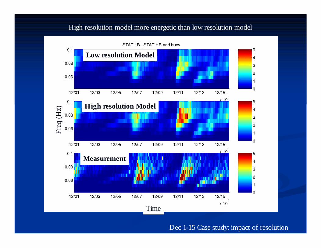
High resolution model more energetic than low resolution model

Dec 1-15 Case study: impact of resolution

Time

Freq

(Hz)

Wav

e H

eigh

t (m

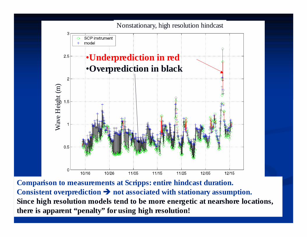
)•Underprediction in red•Overprediction in black

Comparison to measurements at Scripps: entire hindcast duration.Consistent overprediction è not associated with stationary assumption.Since high resolution models tend to be more energetic at nearshore locations, there is apparent “penalty” for using high resolution!

Nonstationary, high resolution hindcast

Example low resolution model result

Example high resolution model result

The two high resolution models tend to allow more energy past the islands into the nearshore areas.


Example lowresolution model result

Example highresolution model result

The two high resolution models tend to allow more energy past the islands into the nearshore areas.


With coarse resolution,•More constriction•More diffusion

Oct. 22Oct. 22--Nov. 8 Case StudyNov. 8 Case Study

Wav

e H

eigh

t (m

)•Underprediction in red•Overprediction in black

“Torry Pines Inner” buoy Oct 22-Nov 11Consistent overprediction è not associated with stationary assumption

Nearshore Location

Oct 22 - Nov 8: study of swell forcing

Time

•SWAN predictions look relatively good at offshore location•Bias the fault of blocking in SWAN?

Wav

e H

eigh

t (m

)

Oct 22 - Nov 8: study of swell forcing

Offshore Location (46047)

Study Oct. 30 1200Z in greater detail

Boundary forcing from WW3 ENP model

Boun

dary

forc

ing

from

CD

IP b

uoy

TPI buoy

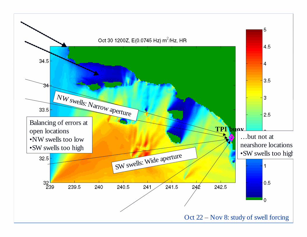
Alarming discrepancy, and a clue!Oct 22 – Nov 8: study of swell forcing

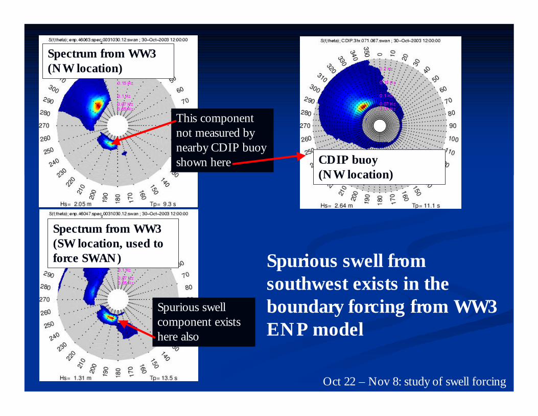
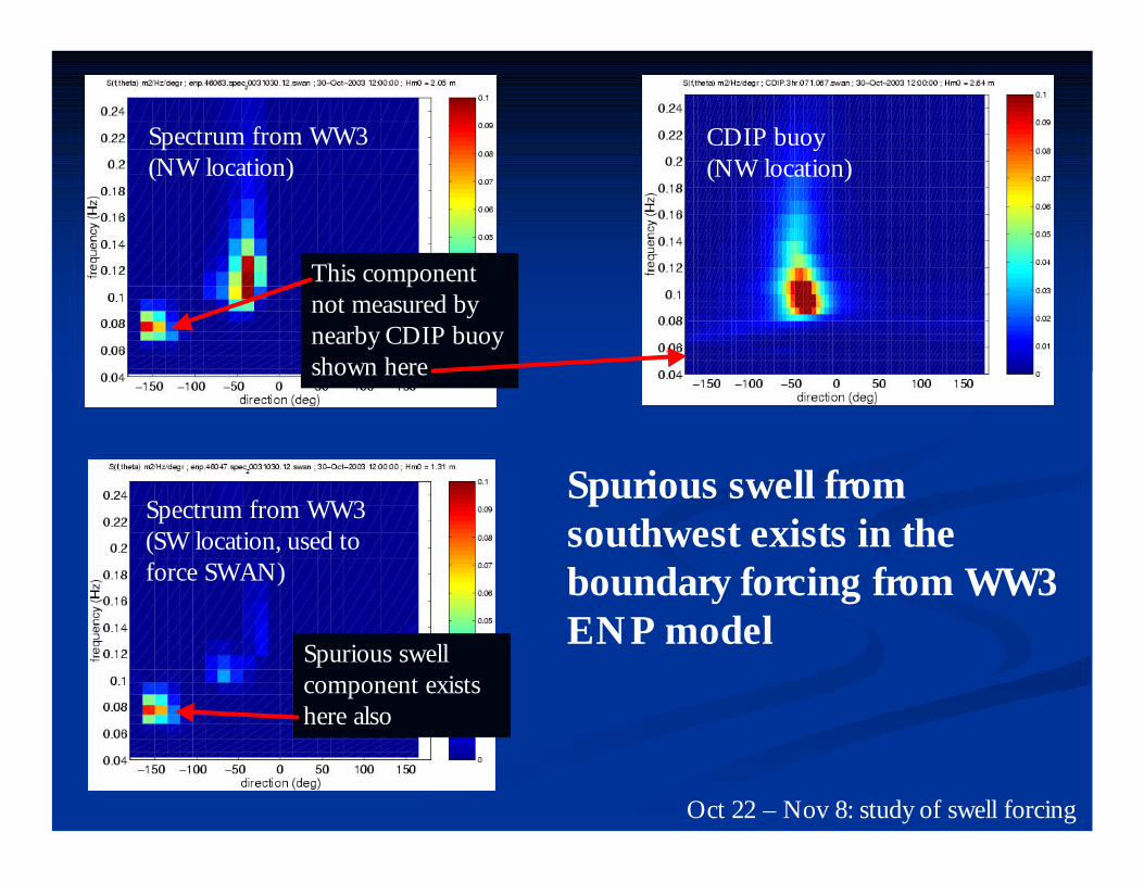
Spectrum from WW3(NW location)

Spectrum from WW3(SW location, used to force SWAN)

CDIP buoy(NW location)

This component not measured by nearby CDIP buoyshown here

Spurious swell component exists here also

Spurious swell from southwest exists in the boundary forcing from WW3 ENP model

Oct 22 – Nov 8: study of swell forcing

•Southwest swells not affected by blocking at these locations•Compare ENP WW3 prediction at 46063 to measurement at 071


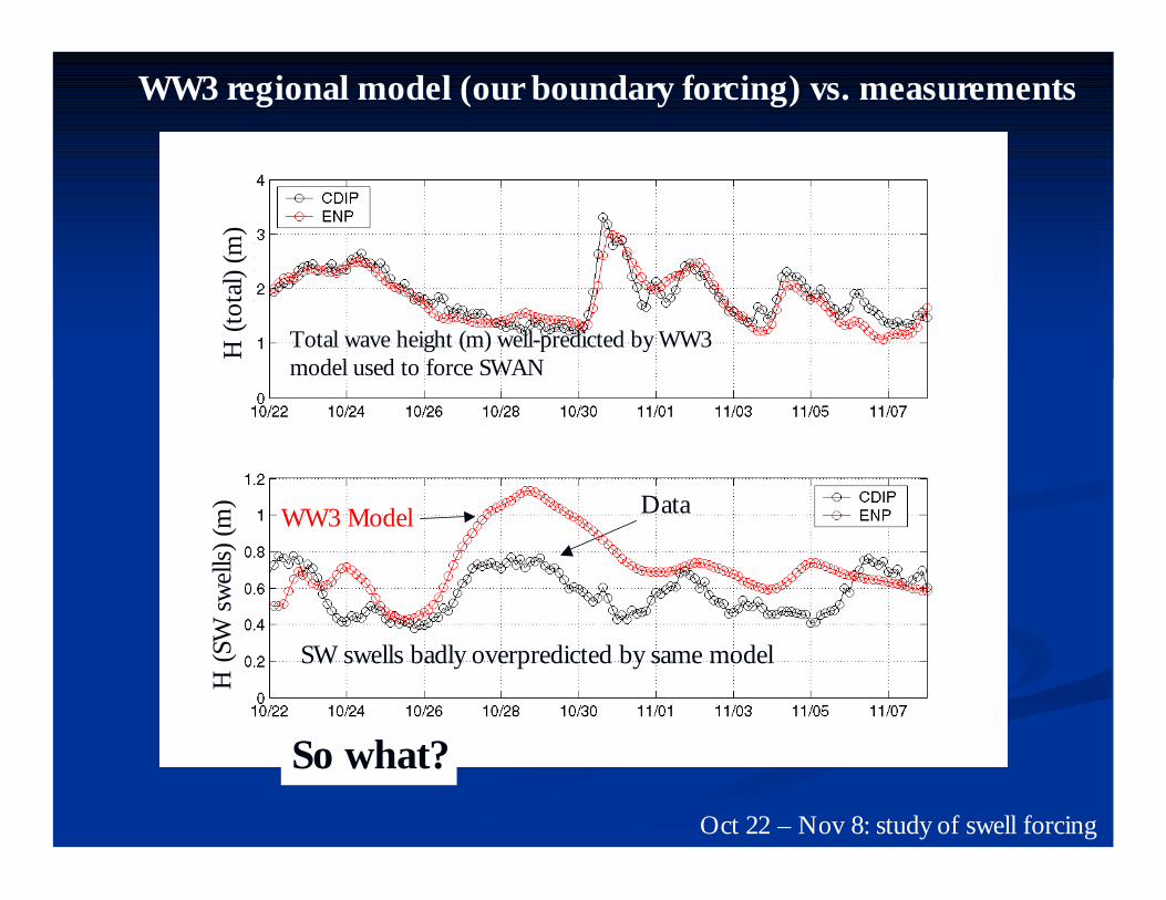
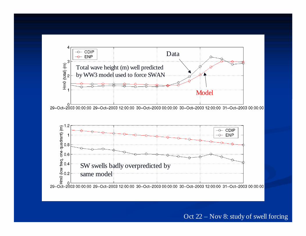
Total wave height (m) well-predicted by WW3 model used to force SWAN

WW3 Model Data

SW swells badly overpredicted by same model


H (t

otal

) (m

)H

(SW

sw

ells)

(m)

So what?

WW3 regional model (our boundary forcing) vs. measurements

TPI buoy


Balancing of errors at open locations•NW swells too low•SW swells too high

…but not at nearshore locations•SW swells too high

NW swells: Narrow aperture

SW swells: Wide aperture

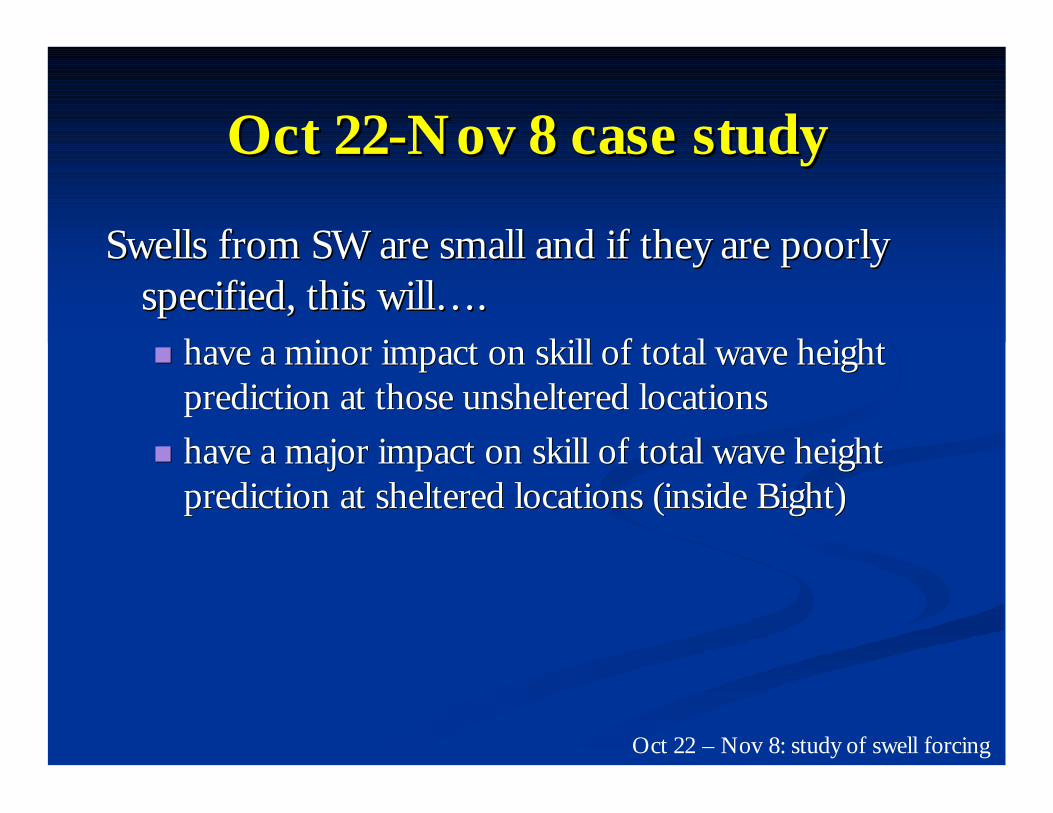
Oct 22Oct 22--Nov 8 case studyNov 8 case study

Swells from SW are small and if they are poorly Swells from SW are small and if they are poorly specified, this will….specified, this will….nn have a minor impact on skill of total wave height have a minor impact on skill of total wave height

prediction at those unsheltered locationsprediction at those unsheltered locationsnn have a major impact on skill of total wave height have a major impact on skill of total wave height

prediction at sheltered locations (inside Bight)prediction at sheltered locations (inside Bight)


DiscussionDiscussion

nn Blindfold realtime system vs. hindcastBlindfold realtime system vs. hindcastnn Model handoffModel handoff

ConclusionsConclusions

nn (SCAL and similar cases) Accuracy of directional (SCAL and similar cases) Accuracy of directional characteristics of boundary forcing criticalcharacteristics of boundary forcing critical

nn SWAN now feasible for high resolution, nonstationary SWAN now feasible for high resolution, nonstationary computationscomputations

nn Coarse (Coarse (∆∆x, x, ∆∆y) y) computations for SCAL (SC1) grid computations for SCAL (SC1) grid èèno penalty in RMS error (and negative trend in bias)no penalty in RMS error (and negative trend in bias)

nn Stationary computations for SCAL (SC1) grid Stationary computations for SCAL (SC1) grid èèpenalty in RMS errorpenalty in RMS error

[a [a pdfpdf of this paper is available, also some hard copies]of this paper is available, also some hard copies]

Some problemsSome problems

nn Garden Sprinkler EffectGarden Sprinkler Effectnn (a side effect of discrete representation of (a side effect of discrete representation of

continuous spectrum)continuous spectrum)

nn Refraction at coarse geographic resolutionRefraction at coarse geographic resolutionnn UnderconvergenceUnderconvergence

Subtle yet significant è problematic, esp. for new SWAN users in Navy è A.I. required?

Result with 10° directional resolution

Wave height (m) predictions from outer SWAN grid, zoomed in on nearshore area

Result with 2°directional resolution

(used as “ground truth”)

Result with 10° directional resolution and Garden Sprinkler

CorrectionDifferent result indicatesGarden Sprinkler Effect(a side effect of discrete representation of continuous spectrum)

Unfortunately, correction is tuned for this “ground

truth” and may not work as well for other cases and it

makes our model conditionally stable.

ClimatologyClimatology

Is this feature real?

Refraction in SWAN

Longitude

•Default settings for numerics•Resolution:

•nx=31•ny=37•nθ=36

Refraction at coarse resolution: Hm0(m) shown

Longitude

•Default settings for numerics•Resolution:

•nx=121•ny=145•nθ=120

Correct garden sprinkler effect using high directional

resolution: this simulation can then be

used as a “ground truth” case for adjusting numerics

Latit

ude

•Limiter on refraction•CDLIM=1.25

•Resolution:•nx=31•ny=37•nθ=36

Longitude

Numerics can be adjusted via a limiter on refraction: this limiter removes the artifact in coarse resolution model

Two cases identical except for method of initializing computations (at each time interval):Dramatic difference in bias suggests stationary computations in SWAN are under-converged.

Convergence in SWAN

H (m

)

Time

H (m

)

SWAN (iteration first guess method #2)

SWAN (iteration first guess method #1)

Overprediction in black Underprediction in red

The End.The End.

Extra slidesExtra slides

SummarySummary

nn Refraction computations at coarse resolutionRefraction computations at coarse resolutionnn Garden Sprinkler Effect Garden Sprinkler Effect

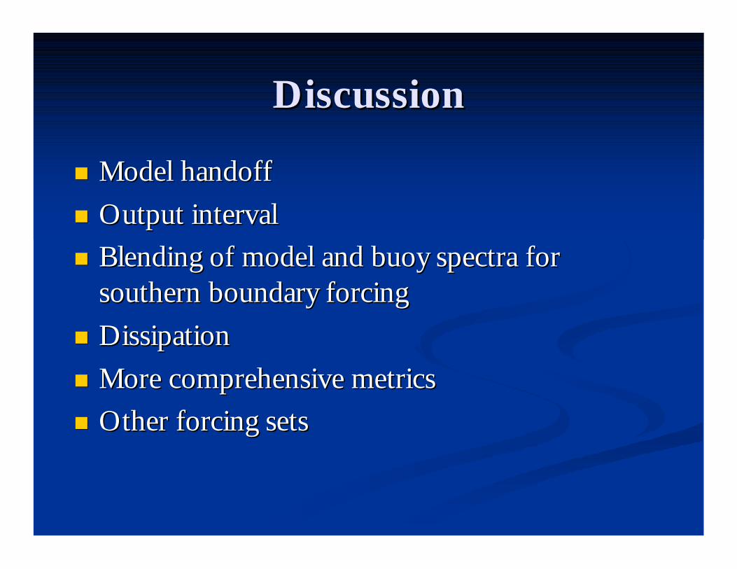
DiscussionDiscussion

nn Model handoffModel handoffnn Output intervalOutput intervalnn Blending of model and buoy spectra for Blending of model and buoy spectra for

southern boundary forcing southern boundary forcing nn DissipationDissipationnn More comprehensive metricsMore comprehensive metricsnn Other forcing setsOther forcing sets

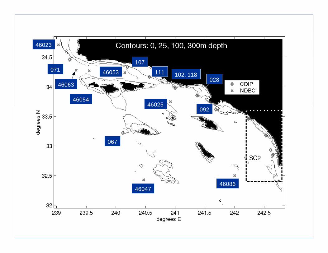
46023

071

46063

46054

46053

46025

102, 118111

107

4604746086

092

028

067

DPT/096

OSO/045

TPO/100

(095)

(101)

(073)

NC

EX

Stu

dy A

rea


1st (outermost) SWAN Nest



2nd SWAN Nest



3rd (innermost) SWAN Nest (corresponds to NCEX region)


Time series comparisons

at three instrument locations


Realtime Time Series Comparisons to Data


Example:

Torrey Pines “Inner buoy”

Frequency (Hz)

Freq

uenc

y (H

z)

Freq

uenc

y (H

z)

E(f

) (m

2/H

z)

Direction (deg)

Direction (deg)

+

=

Measured non-directional spectrum(directional measurement not available near this boundary)

Modeled normalized directional spectrum (from large-scale model)

Directional spectrum for boundary forcing

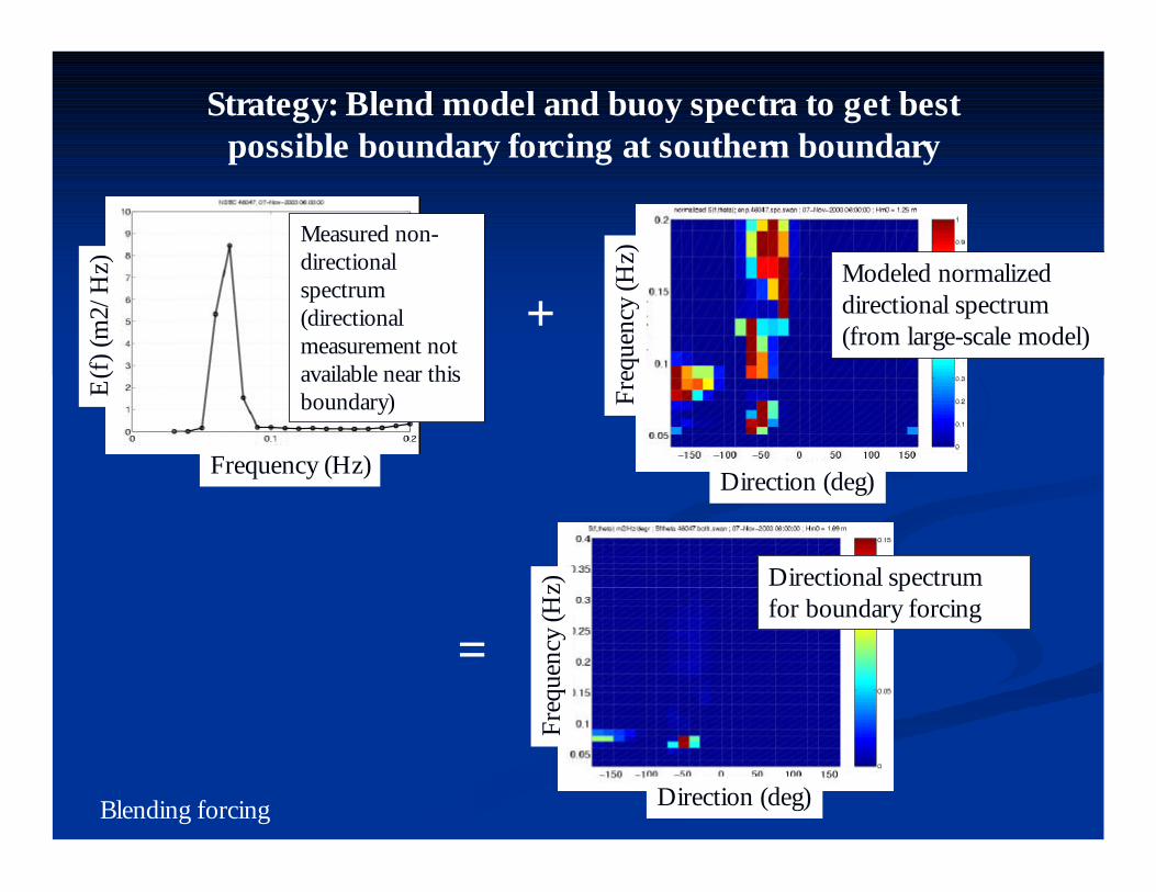
Strategy: Blend model and buoy spectra to get best possible boundary forcing at southern boundary

Blending forcing

Strategy: Blend model and buoy spectra to get best possible boundary forcing at southern boundary:

(Why it does not work.)

Scenario:•Buoy measures strong swell at 0.06 Hz (almost all from northwest, but buoy does not know this)•WW3 model has this strong swell in the wrong frequency bin, so WW3 E(0.06Hz) is weak (one weak swell component from NW and one weak swell from SW). Normalized spectrum at 0.06 Hz show two equal components.•Combining spectra, we get a medium swell from NW and medium swell from SW•Swell from NW is irrelevant to NCEX area (it is blocked)•Swell from SW is too high in boundary forcing and is overpredicted by SWAN at NCEX area.

Blending forcing

Total wave height (m) well predicted by WW3 model used to force SWAN

Model

Data

SW swells badly overpredicted by same model



Wav

e H

eigh

t (m

)

SWAN predictions look good at offshore location.


Freq

(Hz)

Freq

(Hz)

Date

TPI buoy


Omit this slide because wrong color scheme (STAT should be plotted red) Dec 1-15 Case study: stationary assumption

Swells in STAT model too early

November 20November 20--30 Case30 Case

Dana Point Buoy

E(0.13Hz) shown (m2/Hz) from stationary hindcast Nov

20-

30 T

est C

ase:

too

muc

h w

ind

sea

getti

ng to

nea

rsho

re a

reas

Wav

e H

eigh

t (m

)

Dana Point Buoy•Underprediction by model•Overprediction by model

Study Nov. 25 2100Z in greater detail Nov

20-

30 T

est C

ase:

too

muc

h w

ind

sea

getti

ng to

nea

rsho

re a

reas

Wav

e H

eigh

t (m

)

Positive bias with either mode of computation. Thus, we can use stationary model for diagnostics.

Nov

20-

30 T

est C

ase:

too

muc

h w

ind

sea

getti

ng to

nea

rsho

re a

reas

Overprediction here

Little or no bias here

E(0.13Hz) shown (m2/Hz) from stationary hindcast Nov

20-

30 T

est C

ase:

too

muc

h w

ind

sea

getti

ng to

nea

rsho

re a

reas

Possible explanations for positive Possible explanations for positive bias in Nov 20bias in Nov 20--30 case.30 case.

nn Insufficient blocking by islandsInsufficient blocking by islandsnn Due to incorrect incident wave directionDue to incorrect incident wave directionnn Due to incorrect incident wave directional spreadingDue to incorrect incident wave directional spreadingnn Due to inadequate resolutionDue to inadequate resolution

nn Not enough dissipation of short wave (0.13 Hz) Not enough dissipation of short wave (0.13 Hz) energyenergy

(Requires further study….)

End of slides for November 20End of slides for November 20--30 Case30 Case

Investigation of strange feature caused by refraction in SWAN

•Limiter on refraction•CDLIM=1.5

•Resolution:•nx=31•ny=37•nθ=36

Wave Height (m)

Numerics can be adjusted via a limiter on refraction: this limiter does not quite remove the artifact

Refraction in SWAN


•Default settings for numerics•Refraction back on•Resolution:

•nx=121•ny=145•nθ=36

Wave Height (m)

Can correct using high geographic resolution, but garden sprinkler effect becomes apparent.

Refraction in SWAN

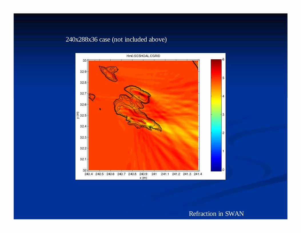
240x288x36 case (not included above)

Refraction in SWAN

Wave height RMS error computations for the wind-forced idealized simulation with stationary computations (simulation with nonstationary computations are taken as ground truth). Cases with forcing corresponding to the Southern California Bight are shown.

Wind-Forced SimulationsBoundary -Forced Simulations

Southern California Bight Cases

Stationary computation causes error because•Instantaneous propagation of swells from boundary•Instantaneous response to winds, infinite duration

Of course, this relation will vary by region/climate, so...

Wav

e H

eigh

t RM

S er

ror (

m)

X (km)

Wave height RMS error computations for the wind-forced idealized simulation with stationary computations (simulation with nonstationary computations are taken as ground truth). Cases with forcing corresponding to the Gulf of Maine are shown.

Wind-Forced Simulations

Boundary -Forced Simulations

Gulf of Maine Cases

Wav

e H

eigh

t RM

S er

ror (

m)

X (km)

Wave height RMS error computations for the wind-forced idealized simulation with stationary computations (simulation with nonstationary computations are taken as ground truth). Cases with wind forcing are shown.

Southern California Bight

Wind-Forced Simulations

Gulf of Maine

Wave height RMS error computations for the boundary-forced idealized simulation with stationary computations (simulation with nonstationary computations are taken as ground truth). Cases with boundary forcing are shown.

Boundary-Forced Simulations

Southern California Bight

Gulf of Maine

Representing the blocking of wave energy by islands, etc.:The impact of geographic resolution

We can simplify problem such that for a given route of wave energy traveling through a region with islands/shoals, there are 4 possible scenarios:

Model is Model is correctcorrect

Model isModel iswrongwrong

Energy is not Energy is not blocked in blocked in wave modelwave model

Model isModel iswrongwrong

Model is Model is correctcorrect

Energy is Energy is blocked in blocked in wave modelwave model

Energy is not Energy is not blocked in real blocked in real worldworld

Energy is Energy is blocked in real blocked in real worldworld

Representing the blocking of wave energy by islands, etc.:The impact of geographic resolution

•For a single geographic location, “route” is defined by direction of approach•Problem is then simply a function of

•permeability α•and accuracy κ, the probability that a given “route” is correctly represented

•7000 realizations with spectra from CDIP buoy 071•Random number generator to determine which of 4 scenarios occurs

Bathymetry by coin toss

Perfect bathymetry

Few islands

Many islands

Expected Error

Nonstationary Model

Stationary Model

Measurement


Time

Freq

(Hz)

E(f

) (m

2 /H

z)

Freq (Hz)

Overprediction occurs for both high resolution and low resolution hindcasts è less likely to be associated with blocking by islands

Data

High resolution model

Low resolution model


Spectrum from WW3(SW location, used to force SWAN)

Spectrum from WW3(NW location)

This component not measured by nearby CDIP buoyshown here

CDIP buoy(NW location)

Spurious swell component exists here also

Spurious swell from southwest exists in the boundary forcing from WW3 ENP model


Also worth noting:The two high resolution models tend to allow more energy past the islands into the nearshore areas.


Example result at a nearshore location

Coarse resolution model

High resolution model

•Refraction disabled•Resolution:

•nx=31•ny=37•nθ=36

Investigation of strange feature

Wave Height (m)

...It is apparently caused by refraction:

LongitudeRefraction in SWAN

Latit

ude


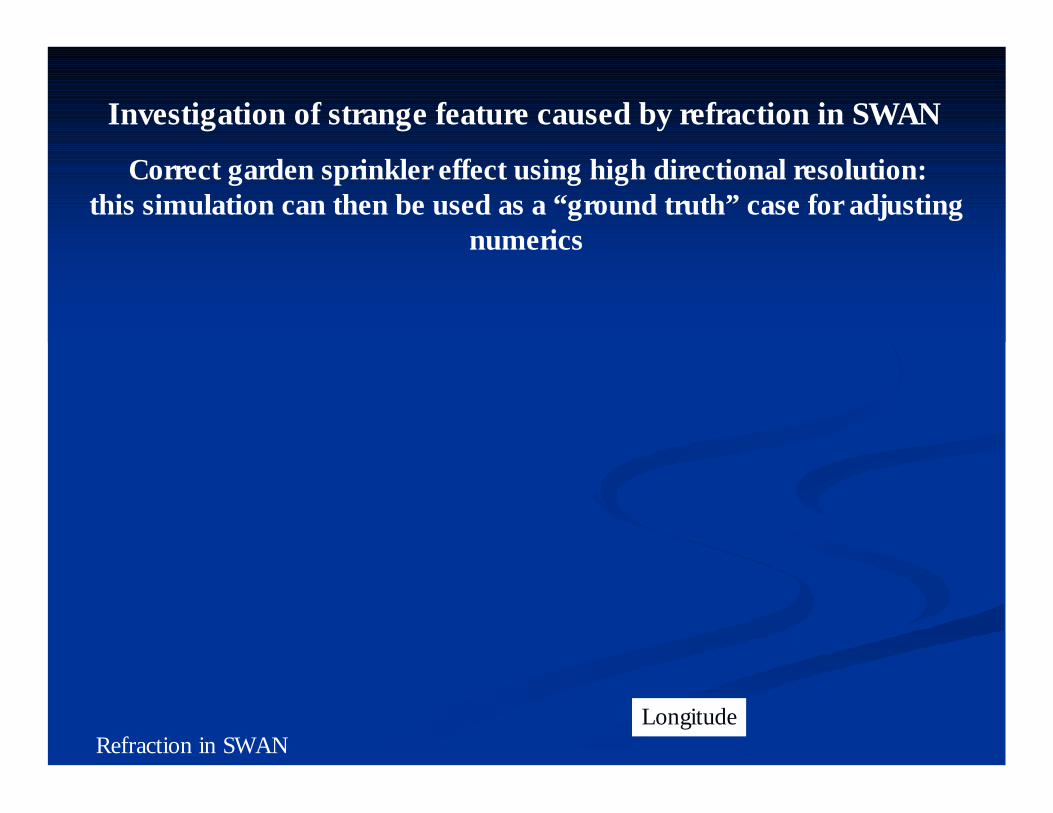
Correct garden sprinkler effect using high directional resolution: this simulation can then be used as a “ground truth” case for adjusting

numerics

LongitudeRefraction in SWAN


…

Refraction in SWAN

Documents

Minimizing errors in sub-regional scale wave modeling · Minimizing errors in sub-regional scale wave modeling: Design of a forecasting system for the Nearshore Canyon Experiment