Embed Size (px)
Citation preview

C'R-189439
Minimizing Structural Vibrations with Input Shaping TM
Final Report for ContractNAS5-32034
Convolve, Inc.January 1995
(NASA-CR-189439) MINIMIZING
STRUCTURAL VIBRATIONS WITH INPUT
SHAPING (TM) Fina| Report(Convolve) 170 p
N95-30786
Unclas
G3139 0058679
https://ntrs.nasa.gov/search.jsp?R=19950024365 2018-08-01T08:57:16+00:00Z

Contents
Background of the Technology ................................................................................................. 1Summary of the Technology ................................................................................................... 2Brief Description of the Drawings ............................................................................................. 5Detailed Description of Developed Technologies .......................................................................... 9
Extra-Insensitive and Specified Insensitivity Input Shapers ................................................ 9Introduction .................................................................................................. 9Vector Diagrams ........................................................................................... 11The Effects of Damping .................................................................................. 12Sensitivity to Errors in Natural Frequency .......................................................... 13Effects of Modeling Errors on the Vector Diagram ............................................... 13Defining Insensitivity .................................................................................... 14Increasing Insensitivity by Relaxing Constraints ................................................. 14Experimental Results ..................................................................................... 16Four-Impulse Extra-Insensitive Shapers ............................................................. 17Extra-Insensitive Shapers with an Arbitrary Number of Humps in the SensitivityCurve .......................................................................................................... 18Specified Insensitivity Shapers ......................................................................... 20
Negative Input Shapers ............................................................................................... 22Introduction .................................................................................................. 22Over-Currenting with Negative Shapers ............................................................. 23Negative ZV (Zero Vibration) Shapers .............................................................. 24Negative ZVD (Zero Vibration & Derivative) Shapers .......................................... 26Negative EI (Extra-Insensitive) Shapers ............................................................. 26Controlling High-Mode Excitation ................................................................... 28Negative Shaper Experimental Results .............................................................. 30
Extra-Insensitive Input Shapers for Controlling Flexible Spacecraft .................................... 31Introduction .................................................................................................. 31Constraint Equation Derivation ........................................................................ 33Input Shaper Comparison ............................................................................... 35Input Shaper Verification ................................................................................ 37
Multiple-Mode Impulse Shaping Sequences .................................................................... 39Introduction .................................................................................................. 39Two-Mode Sequences ..................................................................................... 39Insensitivity to modeling errors ........................................................................ 42Experimental setup ........................................................................................ 42Two-Mode Shaper Experimental Results ............................................................ 44
Input Shapers TM for Digital Systems ............................................................................. 47Introduction ................................................................................................. .47Input Shaping Method .................................................................................... 48Digital Shaper Experimental results .................................................................. 49
Input Shaping TM for Trajectory Following ...................................................................... 51Introduction .................................................................................................. 51Circular Trajectories ....................................................................................... 52Square Trajectories ......................................................................................... 54Improving Shaped Circular Responses ............................................................... 56Improving Shaped Square Responses ................................................................. 56Experimental Results ..................................................................................... 57
Using Different Shapers for Each Axis of Motion ............................................................ 58Reduction of Vibration During Scanning ....................................................................... 58Whole Trajectory Shaping ........................................................................................... 58Implementing Look-up Table for Shaped Trapezoidal Profiles on an LM628/629 .................. 59Shaping Look-up Table for Arbitrary Commands ............................................................ 63Shaping During Emergency Situations ......................................................................... .64Shaping Stepping Motor Systems ................................................................................ 64Shaping controller product .......................................................................................... 64
TuningTrapezoidal, S-Curve, and Parabolic Profiles for Vibration Reduction ....................... 65Introduction .................................................................................................. 65Trapezoidal Velocity Profiles ........................................................................... 65S-Curve Velocity Profiles ............................................................................... 67Parabolic Profiled Trajectories .......................................................................... 69_ures for Selecting the Parameters vmax, amax, jerk for TrapezoidalVelocity Profiles ........................................................................................... 70Procedures for Selecting the Parameters vmax, amax, and jerk for S-CurveVelocity I'roffles ........................................................................................... 7 !Procedures for Selecting the Parameters vmax, amax, and jerk for ParabolicVelocity Profiles ........................................................................................... 72
Input Shapers TM in Closed Loop Systems ...................................................................... 72Miscellaneous Shaping Applications ............................................................................. 74
Figures ................................................................................................................................ 77Appeadix A - Manual f_ Input Shaping GAMS Scripts ............................................................... 116Appendix B - MATLAB Input Shaping TM Toolbox ...................................................................... 155

Executive Summary/Commercialization Results
The result of this contract is a new method of commanding computer controlled machines
to move with improved dynamic performance. This new technology enables machines to
move quickly without spending time waiting for vibrations to settle. This contractgenerated significant research results. These results are now being commercialized foruse within NASA and in the industrial sector.
For example, on March 2, 1995 the Space Shuttle Endeavor will be flying a payload
called MACE (Mid Deck Active Control Experiment). A significant portion of the
MACE experimental program consists of tests of control strategies that involve InputShaping TM. This experiment will validate the use of Input Shaping TM on space-based
systems and structures.
On the commercial front, Convolve, Inc. is currently licensing Input Shaping TM into a
variety of commercial products. As one example, Convolve, Inc. has signed a license to
install Input Shaping TM on a machine that tests computer disk drive read/write heads forSeagate Technology's manufacturing operations. Over one hundred of these test
machines are in service to perform 100% inspection of each head before they are
assembled into computer disk drives. Convolve, Inc.'s software reduced the settle time of
this testing machine from 200 msec to 23 msec. This improvement has significant
ramifications for Seagate's production capacity since many moves are performed in orderto test each head.
In addition to custom applications such as the Seagate machine, Convolve, Inc. is
producing software products based on Input Shaping TM that run on standard controllers
manufactured by two of the leading motion controller manufacturers, Motion Engineering
and Delta Tau Data Systems. These software products consist of two parts. The first is a
software tool that enables a user to monitor his system and configure the shaping
algorithm. The second part is firmware for the motion controllers that implement the
Input Shaping TM technique.
A third software product consists of an automated Input Shaper TM design tool that can be
accessed through a computer dial-up service or through Email on the Internet. This
service will use Convolve's highly optimized Input Shaping TM tools to custom-design
multiple-mode Shaping TM sequences. The fourth tool that was commercialized from the
results obtained under this NASA contract is a MATLAB Toolbox for Input Shaping TM
design and analysis. The fifth tool is a series of GAMS optimization scripts for
generating the most highly optimized Input Shapers TM. These software tools are
invaluable for research and new system development. The GAMS code and the
MATLAB Toolbox have been supplied to NASA as a deliverable under this contract and
are documented in this report.

Background of the Technology
This technology is a method for shaping the inputs to a dynamic system in order to
minimize unwanted dynamics in that system.
Many physical systems must operate dynamically in order to accomplish their intended
functions. However, in the course of their motions, the systems may acquire unwanted
dynamics and vibrations which may be detrimental to their operation. For example,
excessive vibrations in a dynamic system may result in larger than normal stresses and a
premature failure of that system. Alternatively, if the system is designed to operate with a
smooth, non-oscillatory motion, then vibrations may cause unwanted oscillations which
actually prevent the system from achieving its intended purpose, or, at the very least, cause
the system to operate at a significantly slower speed and lower performance level than
originally intended. In addition, the unwanted dynamics may also degrade the performance
of the system, either directly or indirectly, since the system is not exactly following its
intended motion. As a result of these consequences, it is often desired to minimize the
unwanted dynamics and vibrations in a physical system.
There are a number of approaches for achieving this end. One approach relies on
altering the physical system in order to reduce any unwanted dynamics. For example, a
robotic arm may be stiffened in order to reduce the amplitude of any residual vibrations, or
the arm may be dampened so that residual vibrations quickly die out, or its mass be
changed so that the resonant frequency of the arm is moved to a more favorable frequency.
However, it is not always possible to alter the physical system. For example, the system
may be so precisely designed as to be intolerant of the desired changes or it may just be
physically impossible to alter the system, as is the case with a system which is inaccessible.
Even if the system may be altered as desired, the alteration may come with a price - a more
massive system, a larger actuator required to move the system or a more complex system,
to name a few. Another approach relies on using a controller to actively reduce any
unwanted dynamics. However, this approach also has its drawbacks. For example, most
controllers rely on some sort of feedback from the unwanted dynamic and also on a good
model of the system to be controlled, either of which may not always be available. In
addition, controllers may be unacceptably complex, either in terms of the additional
physical elements required to implement the controller or in terms of the time required for
the controller to implement its control algorithm. In particular, fast real-time systems may
be too fast for controllers to be an option.
A third approach, which is the approach considered by this technology, relies on
altering the input to the system in order to reduce the unwanted dynamics. This approach

doesnot rely on physical alterationsto the system,good models of the system to be
controlled,or complexreal-timecalculations.In relatedwork, Singer,et. al. [Singer,Neil
C.; Seering,Warren P. "PreshapingCommand Inputs to ReduceSystem Vibration".ASME Journal of Dynamic Systems,Measurement,and Control. (March 1990) and
Singer,et. al. U.S.patent# 4,916,635,April 10, 1990]showedthatresidualvibration can
be significantly reducedby employing an Input ShapingTM method that uses a simple
system model and requires very little computation. The model consists only of estimates of
the system's natural frequency and damping ratio. Constraints on the system inputs result
in zero residual vibration if the system model is exact. When modeling errors exist, the
shaped inputs keep the residual vibration of the system at a low level that is acceptable for
many applications. Extending the method to systems with more than one modeled resonant
frequency is straightforward[Singer, Neil C. Residual Vibration Reduction in Computer
Controlled Machines. Ph.D. Thesis, Massachusetts Institute of Technology. (Feb. 1989)].
The shaping method works in real time by convolving a desired input with a sequence
of impulses to produce the shaped input function that reduces residual vibration. The
impulse sequence used in the convolution is called an input shaper. Selection of the
number and type of impulses, the impulse amplitudes and their locations in time determine
the amplitude and characteristics of the residual vibration. U.S. patent # 4,916,635
discloses the basic concept of using input shapers, while the current report discloses a
variety of input shapers designed to achieve specific goals. Since this report considers
many different input shapers used for various purposes, the description of the technologies
subdivided into sections, with each section devoted to a specific class of input shapers.
Summary of the Technology
The technology for generating an input to a dynamic system to minimize unwanted
dynamics in the system response includes establishing expressions quantifying the
unwanted dynamics. First constraints which bound the available input to the dynamic
system and second constraints which bound the unwanted dynamics are established, and a
solution which is used to generate the input and allows maximum variation in the physical
system characteristics while still satisfying the fu'st and second constraints is found. The
physical system is controlled based on the input to the physical system, whereby unwanted
dynamics are minimized.
In a second aspect of this technology, the method for generating an input to a dynamic
system to minimize unwanted dynamics in the system response includes establishing
expressions quantifying the unwanted dynamics. First constraints which bound the
available input to the dynamic system and second constraints which bound the unwanted
2

dynamicsareestablished,andasolutionwhich is usedto generatethe input andminimizes
the length of the solution while still satisfyingthe frrst and secondconstraintsis found.
The physical systemis controlled basedon the input to the physical system,wherebyunwanteddynamicsareminimized. In a relatedaspectof this technology,the fin'stand
secondconstraintsaresupplementedby athird constraintboundingvariationsin physical
systemcharacteristics,andasolutionwhich is used to generate the input and minimizes the
length of the solution while still satisfying the first, second and third constraints is found.
In a third aspect of this technology, the method for generating an input to a dynamic
system to minimize unwanted dynamics in the system response includes establishing
expressions quantifying the unwanted dynamics. First constraints which bound the
available input to the dynamic system and second constraints on variation in system
response with variations in the physical system characteristics are established, and a
solution which is used to generate the input and minimizes the length of the solution while
still satisfying the first and second constraints is found. The physical system is controlled
based on the input to the physical system, whereby unwanted dynamics are minimized.
Assuming the physical system is characterized by one or more vibrational modes each
of which has a natural frequency and damping coefficient, and the solution is a sequence of
impulses, then sequence may be defined implicitly, explicitly, or approximately by a set of
equations which is chosen according to the constraints being considered and the desired
characteristics of the sought solution. The sequence of impulses is convolved with an
unshaped input and the result of the convolution is used as input to the dynamic system,
whereby the unwanted dynamics are minimized.
In another aspect of this technology, the method for generating an input to a dynamic
system to minimize unwanted dynamics in a physical system response includes establishing
constraints on a sequence of impulses which minimize the unwanted dynamics. A first
sequence of impulses which satisfy these constraints is determined, and a second sequence
of impulses, which are discretized in location, are then determined. The number of
impulses and locations of the impulses for the second sequence is determined based on the
first sequence, and the amplitudes of the impulses of the second sequence are determined to
satisfy the constraints. The second sequence of impulses is used to generate the input and
the physical system is controlled based on the input to the physical system, whereby
unwanted dynamics are minimized.
This technology is also a method for generating an input to a dynamic physical system
to reduce the deviation between the shape of a trajectory traversed by a point in the physical
system and a pre-selected shape includes establishing constraints on the available inputs to
the dynamic system to define a group of possible inputs and determining an impulse

sequencewhich eliminates unwanteddynamics in the physical system. The impulse
sequenceis convolvedwith eachinput in thegroupof possibleinputs to determineagroup
of shapedinputsandtheshapedinput which minimizesthedeviationbetweentheshapeof
the actual trajectory and the pre-selectedshapeis determined. The physical systemis
controlledbasedon theshapedinput which minimizesthedeviationbetweenthe shapeof
theactualtrajectoryandthepre-selectedshape,wherebythedeviationisminimized.
In anotheraspectof this technology,a methodfor generatingan input to a dynamic
system to minimize unwanted dynamics in the physical system responsecomprises
establishingexpressionsquantifying the unwanteddynamics. First constraints on the
availableinputsto thedynamicsystemareestablishedin orderto def'meagroupof possibleinputs,eachinputin thegroupof possibleinputsis expressedasthecombinationof oneor
moreprimitive input wains, and the primitive input train which minimizes the unwanted
dynamics is determined. The physical system is controlled using the input in the group of
possible inputs which corresponds to the primitive input train which minimizes the
unwanted dynamics, whereby unwanted dynamics are minimized. The primitive input
trains are sequences of impulses, and the group of possible inputs are commonly used
inputs, such as those which generate trapezoidal, s-curve, or parabolic velocity profiles.
In a final aspect of this technology, the method for shaping an arbitrary command input
to a dynamic physical system to reduce unwanted dynamics in the physical system includes
determining a first parameterization for the arbitrary command input and determining an
impulse sequence which eliminates unwanted dynamics in the physical system. The
convolution of the impulse sequence with the arbitrary command input is then expressed
using a second parameterization, which is based on the fin'st parameterization, and the input
to the physical system is controlled based on the second parameterization, whereby
unwanted dynamics in the physical system are minimized.
4

Brief Description of the Drawings
FIGS. la, lb and lc illustrate the convolution of an unshaped system input with a
sequence of impulses to produce a shaped system input;
FIGS. 2a and 2b illustrate the correspondence between an impulse sequence and its
vector diagram;
FIGS. 3a, 3b and 3c illustrate the correspondence between a vector diagram and its
time domain representation of vibration;
FIGS. 4a and 4b illustrate the scaling effect of a damping coefficient;
FIG. 5a illustrates a vector diagram for a three-impulse sequence;
FIG. 5b graphs residual vibration versus normalized modeling error for the three-
impulse sequence of FIG. 5a;
FIG. 6a illustrates a vector diagram for an asymmetric three-impulse sequence;
FIG. 6b graphs residual vibration versus normalized modeling error for the three-
impulse sequence of FIG. 6a;
FIG. 7 graphs residual vibration versus normalized modeling error for two different
three-impulse sequences, and illustrates the allowable normalized modeling error for two
different values of insensitivity;
FIG. 8 is a graph of table position versus time for shaped and unshaped inputs;
FIG. 9 is a graph of the experimental and theoretical residual vibration versus
normalized modeling error for the case of V=0.05;
FIG. 10 is a graph of the experimental and theoretical residual vibration versus
normalized modeling error for the case of V=0.10;
FIG. 11 graphs residual vibrations versus normalized frequency for a four-impulse
sequence;
FIG. 12 graphs the amplitude of the first impulse of a multi-impulse sequence as a
function of insensitivity and damping coefficient;
FIG. 13 graphs the location of the second impulse of a multi-impulse sequence as a
function of insensitivity and damping coefficient;
FIGS. 14a, 14b and 14c illustrate over-currenting caused by impulse sequences
containing negative impulses;
FIGS. 15, 16 and 17 graph the residual vibration versus normalized frequency for
different impulse sequences;
FIG. 18 graphs the length of an impulse sequence versus the peak partial sum;
FIG. 19 graphs the residual vibration versus normalized frequency for three different
impulse sequences with a peak partial sum of one;
FIGS. 20 and 21 graph the residual vibration versus normalized frequency for two

differentimpulsesequences;
FIG. 22 graphsthe residualvibration versusnormalizedfrequency for an impulse
sequenceusedwith a low-passfilter;,
FIG. 23graphsencoderpositionversustime for shapedandunshapedinputs;
FIG.24 graphsencoderpositionversustime for four different impulsesequences;
FIG.25 illustratesa simplesystemmodel;
FIGS.26a,26b and26cillustratetheconvolutionof asysteminput with a sequenceof
impulsestoproducea shapedsysteminput of constantmagnitude;
FIG.27 graphsresidualvibrationversusfrequencyfor different impulsesequences;
FIGS. 28a and 28b graphposition versus time for various impulse sequencesand
springconstants;
FIG. 29 graphs magnitudeversus frequency for the vibration resulting from an
unshapedinput;
FIG. 30graphstablepositionversustimefor anunshapedanda shapedinput;
FIG. 31 illustratesa symmetric,five impulsesequencewhich reducesvibrations fortwo differentmodes;
FIG. 32 graphstheresidualvibration versussystemfrequencyfor a sequenceof the
typeshownin FIG. 31;
FIG. 33illustratestheCMSsystem;
FIG. 34graphstheresidualvibrationversusfrequencyfor anine-impulseandfifteen-impulsesequence;
FIG. 35graphsencoderpositionversustime;
FIGS. 36a, 36b, 36c, and 36d graph laser derived position versus time for four
differentimpulsesequences;
FIG. 37 graphsthe magnitudeof the FFT versus frequency for a shapedand an
unshapedinput;FIG. 38 illustrates a situation in which a three-impulsesequencedoes not fit the
discretespacingof asystem;FIG. 39 graphsresidualvibr',itionsversussystemfrequencyfor four different impulse
sequences;FIG. 40a illustrates how a three-impulsesequencewhich does not fit the discrete
spacingof a system;
FIG. 40b illustratesafive-impulsesequence,basedon thethree-impulsesequenceof
FIG.40a,which doesfit thediscretespacingof asystem;
FIG. 41illustratesanexperimentalconfigurationwith twomodesof vibration;
FIGS.42,43,44and45graphtablepositionasafunctionof timefor variousinputs;

FIG. 46 illustrates a two-mode model for a flexible system under PD control;
FIG. 47 graphs the trajectories resulting from an unshaped and a shaped input;
FIG. 48 graphs the command amplitude versus time for four different commands;
FIG. 49 graphs radius envelope versus vibration for different inputs and damping
coefficients;
FIG. 50 graphs radius envelope versus departure angle for various inputs;
FIG. 51 graphs radius envelope versus frequency for various inputs;
FIG. 52 graphs the trajectories resulting from an unshaped and a shaped input;
FIG. 53 graphs the command amplitude versus time for various inputs;
FIG. 54 graphs mean error versus cycles per square for various input and damping
coefficients;
FIG. 55 graphs the trajectories resulting from an unshaped and a shaped input for a
departure angle of thirty degrees;
FIG. 56 graphs mean error versus departure angle for various inputs;
FIG. 57 graphs mean error versus frequency for various inputs;
FIG. 58 graphs the trajectory resulting from using a shaped input designed for a circle
of increased radius and allowing for transients;
FIG.59 graphs tracking error versus time for a shaped input used to trace a square;
FIG. 60 illustrates a device used to record different trajectories;
FIG. 61 illustrates the trajectory produced by an unshaped input;
FIG. 62 illustrates the trajectory produced by a shaped input;
FIG. 63 illustrates the trajectory produced by an unshaped input when an endpoint
mass is added to the device of FIG. 60;
FIG. 64 illustrates the trajectory produced by a shaped input when an endpoint mass is
added to the device of FIG. 60;
FIG. 65 graphs velocity versus time for an unshaped and shaped trapezoidal velocity
profile;
FIGS. 66a and 66b illustrate that the superposition of four shaped acceleration steps
yields a shaped trapezoidal velocity profile;
FIG. 67 graphs pullout torque versus step rate for a stepper motor;
FIGS. 68a and 68b illustrate a trapezoidal velocity profile and its corresponding
acceleration profile;
FIGS. 69a, 69b, 69c and 69d illustrate that the acceleration prof'de of FIG. 68b may be
decomposed into the convolution of a step function with two sequences of two impulses
each;
FIGS. 70 and 71 graph residual vibration versus frequency for different inputs;
7

FIGS. 72a,72b and72c illustrate an s-curvevelocity profile and its corresponding
accelerationandjerk profiles;FIGS.73a,73b,73c,73d and73eillustrate that the jerk profile of FIG. 72c may be
decomposedinto theconvolutionof a stepfunction with threesequencesof two impulseseach;
FIG.74graphsresidualvibrationversusfrequencyfor different inputs;andFIGS. 75a,75b and75c illustrate a parabolicvelocity profile and its corresponding
accelerationandjerk profiles;FIG.76 is ablockdiagramof aclosedloop systemwith aninternalinput shaper,
FIG. 77 is a block diagramof aclosedloop systemwith aninternal input shaperanda
compensatingfilter,
FIG.78 is ablockdiagramof aclosedloop systemwith anexternalinput shaper;,FIG.79 is a schematicillustration of the technology disclosed herein.

Detailed Description of Developed Technologies
Extra-Insensitive and Specified Insensitivity Input Shapers
Introduction
An early pre-cursor of Input Shaping TM was the use of posicast control by O.J.M.
Smith [Smith, O.J.M. Feedback Control Systems. McGraw-Hill Book Company, Inc.,
New York (1958)]. This technique breaks a step input into two smaller steps, one of
which is delayed in time. The result is a reduced settling time for the system. Wiederrich
and Roth [Wiederrich, J. L.; Roth B., "Dynamic Synthesis of Cams Using Finite
Trigonometric Series". Journal of Engineering for Industry (Feb. 1975)] shaped cam
profiles to control the harmonic content of the imposed vibration. Their methods reduced
steady-state vibration and assured the accuracy of their simple model.
Optimal control approaches have been used to generate input profiles for commanding
vibratory systems. Junkins, Turner, Chun, and luang have made considerable progress
toward practical solutions of the optimal control formulation for flexible systems[Junkins,
John L.; Turner, James D. "Optimal Spacecraft Rotational Maneuvers". Elsevier Science
Publishers, New York. (1986) , Chun, Hon M.; Turner, James D.; Juang, Jer-Nan.
"Disturbance-Accommodating Tracking Maneuvers of Flexible Spacecraft". Journal of the
Astronautical Sciences 33, 2. (April-June, 1985)]. Gupta [Gupta, Narendra K.
"Frequency-Shaped Cost Functionals: Extension of Linear-Quadratic". Journal of
Guidance and Control 3, 6 (Nov.-Dec, 1980)], and Junldns and Turner[Junkins, John L.;
Turner, James D. "Optimal Spacecraft Rotational Maneuvers". Elsevier Science Publishers,
New York. (1986)] included frequency shaping terms in their optimal formulation.
Farrenkopf[Farrenkopf, R. L. "Optimal Open-Loop Maneuver Profiles for Flexible
Spacecraft". Journal of Guidance and Control 2, 6. (Nov.-Dec., 1979)] developed velocity
shaping techniques for flexible spacecraft. Swigert[Swigert, C. J. "Shaped Torque
Techniques". Journal of Guidance and Control 3, 5 (Sep.-Oct., 1980)] demonstrated that
torque shaping can be implemented on systems which modally decompose into second-
order harmonic oscillators.
Singer and Seering[Singer, Neil C.; Seering, Warren P. "Preshaping Command Inputs
to Reduce System Vibration". ASME Journal of Dynamic Systems, Measurement, and
Control. (March 1990)] showed that residual vibration can be significantly reduced by
employing an Input Shaping TM method that uses a simple system model and requires very
little computation. The model consists only of estimates of the system's natural frequency

anddampingratio. Constraintson thesysteminputsresultin zeroresidualvibration if the
systemmodel is exact. Whenmodelingerrorsexist, the shapedinputs keeptheresidual
vibrationof thesystemat a low level thatis acceptablefor manyapplications. Thereis a
straightforwardmannerto extendthis method to systemswith more thanone modeled
resonantfrequency[Singer,Neil C. ResidualVibrationReductionin ComputerControlled
Machines.Ph.D.Thesis,MassachusettsInstituteof Technology.(Feb.1989)].
Theshapingmethodworksin realtime by convolvinga desiredinput with a sequence
of impulses to producethe shapedinput function that reducesresidual vibration. The
impulsesequenceusedin theconvolution is calledan input shaper. For example,if it is
desiredto movea systemfrom onepoint to another,(a stepchangein position) then the
convolution of the stepfunction with a sequenceof impulses results in a shapedinput
whichis a seriesof steps,or astaircase.Similarly, if aconstantrampinput iscommanded,
theshapedinput will bearampwhoseslopechangesvalueasafunction of time. Insteadof giving thesystemthesteporrampinput,thesystemis giventheshapedinput. Selection
of the impulse amplitudes and locations in time determine the amplitude of residualvibration.
The commanded input is not limited to steps and ramps. Rather, any command
function can be shaped with an impulse sequence. FIG. la depicts a general input which is
convolved with the impulse sequence of FIG. lb. The resulting shaped input is shown as
the solid line in FIG. lc; while the dotted and dashed lines are the two components arising
from each of the two impulses of FIG. lb. Sequences containing three impulses have been
shown to yield particularly effective system inputs (when convolved with system
commands) both in terms of vibration suppression and response time. The shaping method
is effective in reducing vibration in both open and closed loop systems.
This section extends the basic Input Shaping TM technique of Singer and Seering and
concentrates on generating different impulse sequences to be used in the convolution that
produces the vibration-reducing inputs. Unlike the time domain analysis presented in
references [Singer, Neil C. Residual Vibration Reduction in Computer Controlled
Machines. Ph.D. Thesis, Massachusetts Institute of Technology. (Feb. 1989), Singer,
Neil C.; Seering, Warren P. "Preshaping Command Inputs to Reduce System Vibration".
ASME Journal of Dynamic Systems, Measurement, and Control. (March 1990)], this work
uses vector diagrams, which are graphical representations of impulse sequences, to
generate and evaluate the vibration-reducing characteristics of impulse sequences. By
relaxing the constraints used by Singer and Seering, a variety of sequences can be
generated that give better performance than those reported previously.
10

Vector Diagrams
To understand the results presented in this section, one must be familiar with the vector
diagram representation of vibration and its use in creating shaped inputs. An explanation of
vector diagram methods was presented in [Singhose, William E. "Shaping Inputs to
Reduce Residual Vibration: a Vector Diagram Approach". M1T Artificial Intelligence Lab
Memo No. 1223. (March, 1990) ] and will be summarized here.
A vector diagram is a graphical representation of an impulse sequence in polar
coordinates (r-0 space). A vector diagram is created by setting r equal to the amplitude of
an impulse and by setting 0 = coT, where co (rad/sec) is a chosen frequency and T is the
time location of the impulse. FIG. 2a shows a typical impulse sequence and FIG. 2b
shows the corresponding vector diagram.
Vector diagrams become useful tools for producing vibration-reducing impulse
sequences when co is set equal to the best estimate of a natural frequency, o)sys, of a
system and the time of the first impulse is set to zero (T1 = 0). When a vector diagram is
created in this manner, the amplitude of the resultant, A R, is proportional to the amplitude
of residual vibration of a system driven by a step convolved with the impulse sequence.
The angle of the resultant is the phase of the vibration relative to the system response to an
impulse at time zero.
Because arbitrary inputs can be built as sums of steps, the amplitude of A R is a
measure of system response to arbitrary inputs. This result enables us to determine
residual vibration geometrically; the residual vibration is calculated by geometrically
summing the vectors on the vector diagram. FIG. 3a shows the vector diagram
representation for the resultant vibration of a second order undamped system. FIG. 3b
shows the time domain representation of each component of the vibration, and FIG. 3c
shows the time domain representation of the resultant. On a vector diagram, vibration
appears as a vector, whereas, in the time domain, vibration appears as a sinusoid.
We can use the vector diagram to generate impulse sequences that yield vibration-
free system response. To do this, we place n arbitrary vectors on a vector diagram and
then cancel the resultant of the first n vectors with an n+lst vector. When the n+l vectors
are converted into an impulse sequence, and the sequence is convolved with a desired
system input, the resulting shaped input will cause no residual vibration when applied to a
system with natural frequency co. Additionally, if the sum of impulse amplitudes is
normalized to one, the system will stop at the commanded setpoint.
The magnitude, An+ l, and angle, 0n+ 1, of the canceling vector are given by:
IA*+ll = 41R_l 2 + 11_12 0n+l ----_ + tan'l -R-'_'x (1)
11

whereRx andRy arethehorizontalandverticalcomponentsof theresultant.Thesecomponentsaregivenby
Rx-- icos0i Ry-- i___iAisin{}i (2)
where A i and 0i are the magnitude and angles of the n vectors to be canceUcd.
Th¢ Effects of Damping
When the system has viscous damping, the vector diagram representation of vibration must
be modified in two ways. First, we must use the damped natural frequency for plotting the
vector diagram. This corresponds to using:
e= coI (3)
where _ isthedamping coefficient.
Second, the amplitudes of the vectors must be scaled to account for damping. As
time progresses, the amplitude of response decays; therefore, the amplitude of the canceling
vector decreases. For example, if we give a system an impulse with amplitude A1, at time
zero, the single impulse, A 2, that will cancel the system's vibration is located x radians
(180o) out of phase with the first impulse, but it has a smaller amplitude as shown in
FIGS. 4a and 4b. If a system has a damping ratio of 4, then the amplitude of the second
impulse is:
A 2 = Ale-_c0T = Ale-_'0 (4)
where 0 is given by Eq. 3 and
_' = _ /(1-_2)1/2 (5)
We define the effective amplitude, LAefid, of an impulse, A, occurring at time T to
be the amplitude of an impulse occurring at time zero whose vibratory response would
decay to the amplitude of response caused by A at time T. Written in equation form, the
effective amplitude of a vector is:IAI
lAd e-;'0 (6)
When we cancel n vectors with an n+lst vector on a vector diagram to create a
vibration-eliminating impulse sequence, we must use Eq. 3 to determine the angles of the
vectors and assign each of the n vectors an effective amplitude according to Eq. 6 before
using Eqs. 1 to solve for the n+lst vector. When we include the effects of damping, the
equations describing the n+lst canceling vector are:
= (e'_ '0"*') _41Rx12+ IRy_Z On+t= X + tan"1 "lxx_R_r }IAn+II
where Rx and Ry are given by:
(7)
12

R x = _l_,effcosO i
n
Ry = i_Ai_in0i(8)
Sensitivity to Errors in Natural Frequency
It is possible to create an infinite number of vibration-reducing input functions with the
vector diagram tool. The "best" would seem to be the one that works most effectively on
real systems. Because there will always be some error in the estimate of natural frequency
for any system, the sensitivity of the shaped input to modeling errors is important. When
the system model is not exact, some residual vibration will occur when the system is
moved with the shaped inputs. A plot of the vibration versus error in estimated natural
frequency for a three-impulse sequence developed by Singer and Seering is shown in FIG.
5b and the corresponding vector diagram is shown in FIG. 5a. This impulse sequence
produces a system response that is fairly insensitive to errors or changes in the system
parameters. That is, there is relatively little vibration in the system even when the resonant
frequency estimate is off by 15% as shown.
Effects of Modeling Errors on the Vector Diam'arn
The sensitivity curve shown in FIG. 5b can be obtained directly from a vector diagram if
we analyze how a modeling error changes the diagram. When the natural frequency of a
system differs from the assumed natural frequency, the error can be represented on a vector
diagram by shifting each vector through an angle (_. If COsys is the actual natural frequency
of the system and co is the modeling frequency, then the error in frequency is to - tosys"
The angle through which the vectors are shifted, ¢, is related to the frequency error by the
equation:
= (to - C0sys)T (9)
The error in modeling causes a non-zero resultant to be formed on the vector
diagram if the vectors were determined by Eqs. 1. The resultant that is formed represents
the vibration that is induced by the error in frequency.
Given that modeling errors cause a resultant, Rer r, on a vector diagram, we can
compare the sensitivity of different input functions to modeling errors by plotting the
amplitude of Rerr versus the error in frequency. If we plot a sensitivity curve like the one
shown in FIG. 5b, we can determine how much vibration will result from a given error in
estimated frequency. To make a sensitivity curve, we must develop an expression for the
amplitude of the resultant as a function of the error in frequency (co - COsys). This has been
done previously[Singhose, William E. "A Vector Diagram Approach to Shaping Inputs for
Vibration Reduction". MIT Artificial Intelligence Lab Memo No. 1223. (March, 1990) ],
13
and the relation is:
IP.. = IR l +
where:
Rxc_r = _AicflCOS(0i-_i)
Aieff= Ai
e_;'Coi- tO
co- o3__= to 0i
Ry_ = _A_fpin(ei--_i)
(10)
(11)
(12)
(13)
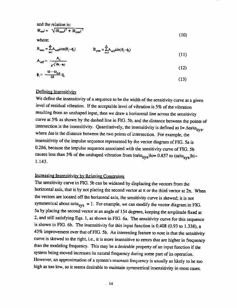
Defining Insensitivi _ty
We define the insensitivity of a sequence to be the width of the sensitivity curve at a given
level of residual vibration. If the acceptable level of vibration is 5% of the vibration
resulting from an unshaped input, then we draw a horizontal line across the sensitivity
curve at 5% as shown by the dashed line in FIG. 5b, and the distance between the points of
intersection is the insensitivity. Quantitatively, the insensitivity is defined as I= At0/tosy s,
where Aco is the distance between the two points of intersection. For example, the
insensitivity of the impulse sequence represented by the vector diagram of FIG. 5a is
0.286, because the impulse sequence associated with the sensitivity curve of FIG. 5b
causes less than 5% of the unshaped vibration from (m/tOsys)lo= 0.857 to (o)/msys)hi=
1.143.
In_-r_ing Insensitivity by R¢laxing Constraints
The sensitivity curve in FIG. 5b can be widened by displacing the vectors from the
horizontal axis, that is by not placing the second vector at n or the third vector at 2n. When
the vectors are located off the horizontal axis, the sensitivity curve is skewed; it is not
symmetrical about to/C0sy s = 1. For example, we can modify the vector diagram in FIG.
5a by placing the second vector at an angle of 154 degrees, keeping the amplitude fixed at
2, and still satisfying Eqs. 1, as shown in FIG. 6a. The sensitivity curve for this sequence
is shown in FIG. 6b. The insensitivity for this input function is 0.408 (0.93 to 1.338), a
43% improvement over that of FIG. 5b. An interesting feature to note is that the sensitivity
curve is skewed to the right, i.e., it is more insensitive to errors that are higher in frequency
than the modeling frequency. This may be a desirable property of an input function if the
system being moved increases its natural frequency during some part of its operation.
However, an approximation of a system's resonant frequency is usually as likely to be too
high as too low, so it seems desirable to maintain symmetrical insensitivity in most cases.
14

To increase insensitivity and still maintain a symmetrical sensitivity curve, we can
relax Singer's constraint of zero vibration when the system model is exact. Any system
model will have some amount of approximation, so giving up this strict constraint is
reasonable. Insensitivity is increased significantly if we reformulate the constraints in the
following way. Pick an allowable level of residual vibration, V. Then, calculate
amplitudes for the impulses at 0 = 0, _, and 2_ such that the residual vibration equals V
when (OR0sy s = 1. Furthermore, require the sensitivity curve to drop to zero on either side
of o)/a)sy s = 1.
From the above conditions, we can derive the three-impulse sequence that yields the
maximum insensitivity for a given vibration limit. The sensitivity curve will be constrained
to be symmetrical about the modeling frequency, this means the angle of the third vector,
03 , is always twice the angle of the second vector, 0 2 . In equation form:
0 3 = 20 2 (14)
When the resultant at the modeling frequency is set equal to the vibration limit, V, we have:
tAll - tA21 + IA31 = V(LAll + LA21+ tA3 I) (15)
The value of tA21 is subtracted from the left side of Eq. 15 because the vector A 2 points in
the opposite direction ofA 1 and A 3 on the vector diagram. We have arbitrarily set IAll
equal to one, so Eq. 15 reduces to:
(1 - v )(1 + I&0IA2I =
(1 + v) (16)
Because we are forcing the sensitivity curve to drop to zero on either side of oYO_sy s
= 1, the resultant on the vector diagram must equal zero for the values of 0+a and 0-13,
where o_and 13are some unknown deviations from the angle corresponding to o.7COsys = 1.
In equation form this constraint is:
0 = 1 + IA21cos(02+a)+ IA31cos(03+2(x)
0 = IA21sin(02+a) + IA31sin(03+2o0
0 = 1 + IA21cos(02-13)+ IA31cos(03-2_)
0 = IA21sin(02- _) + IA3lsin(03-213)
(17)
(18)
(19)
(20)
Eqs. 14 and 16-20 are six equations with seven unknowns, (A2, A3, 0 2 , 0 3, (z, 13and
V). Neglecting damping and solving the equations in terms of V, we obtain the following
values for the extra-insensitive sequence we were seeking:
IAII I+V I-V I+V- IA21 = _ IA3I =4 42 (21)
01=0 02=_x 03=2_
If we examine the sensitivity curves for the above sequence, we discover that when
the vibration limit is increased, insensitivity improves significantly. The insensitivity is
15

0.399 when V = 0.05, a 39% improvement over Singer's three-impulse sequence of FIG.
5a. The insensitivity further increases from 0.399 to 0.561 when V is increased from 0.05
to 0.10, as shown in FIG. 7.
When the system has viscous damping, the constraint equations cannot be solved in
closed form. Fortunately, the equations containing damping terms that are analogous to
Eqs. 14-20 can be solved numerically to obtain the impulse sequence as a function of two
variables, _ and V. Numerical solutions were calculated for 0 < _ < 0.3 and 0 < V __.0.15.
A surface was fit to the data and the following description of the extra-insensitive sequence
in the time domain was obtained:
AI= 0.2497 + 0.2496V + 0.8001_+ 1.233V_ + 0.4960_2+3.173V42
A2 = 1 - (AI+A3)
A3 = 0.2515 + 0.2147V - 0.83254 + 1.415V_ + 0.851842 - 4.901V42
T1 = 0 (22)
T2 =(0.5000 + 0.4616V_ + 4.262V_2 + 1.756V_3
+ 8.578V2_ - 108.6V2_2 + 337.0V2_3 ) T d
T3-T d
where, T d is the period of damped vibration:2_
ra ; _ (23)
ff we examine the sensitivity curves for the above sequence, we discover that
damping increases the insensitivity to modeling errors. For example, the undamped
sequence based on V -- 5% has an insensitivity of 0.399 while the sequence corresponding
to V = 5% and _ = 0.1 has an insensitivity of 0.470, an 18% improvement. When the
damped sequence is used, the frequencies at which the sensitivity goes to zero are more
distant from the modeling frequency and the sensitivity curves are skewed toward the
higher frequencies.
Exp_ental Results
Tests were performed on the assembly robot described in reference[Vaaler, Erik; Seering,
Warren P., "Design of a Cartesian Robot". Presented at the winter annual meeting of the
ASME (1986)]. A steel beam with a mass at one end was attached to a turntable on the
robot base. The table was driven by a DC motor under PD control and its position was
measured by an optical encoder.
When the table was given a step input in position, large oscillations were induced in
the beam-mass system. The solid line of FIG. 8 shows a typical system response to a step
input. The system parameters were determined by examining the data from a step
16
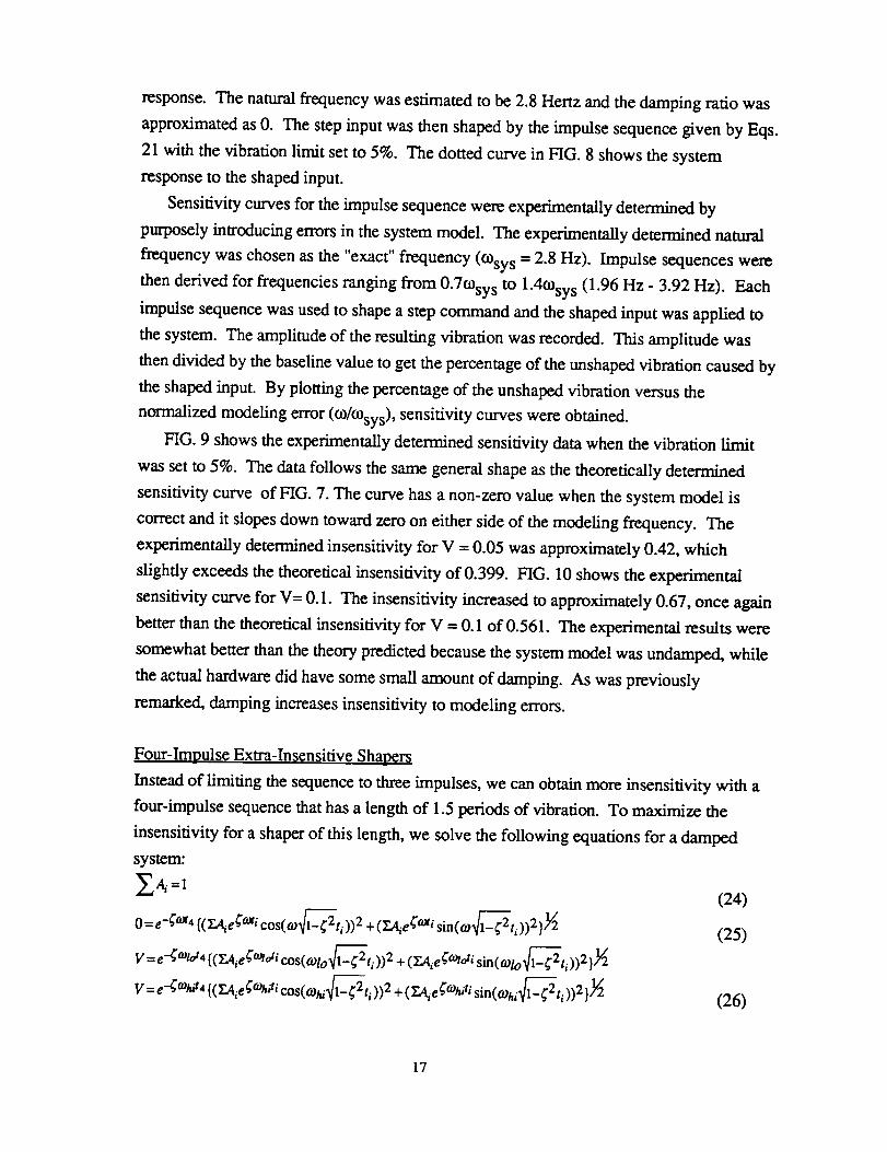
response.Thenaturalfrequencywasestimatedto be2.8Hertzandthedampingratio was
approximatedas0. Thestepinput wasthenshapedby theimpulsesequencegiven byEqs.
21with thevibrationlimit setto 5%. Thedottedcurvein FIG. 8 showsthesystem
responseto theshapedinput.
Sensitivitycurvesfor theimpulsesequencewereexperimentallydeterminedby
purposelyintroducingerrorsin thesystemmodel. Theexperimentallydeterminednatural
frequencywaschosenasthe"exact"frequency(COsys= 2.8 Hz). Impulse sequences were
then derived for frequencies ranging from 0.7Osy s to 1.4Oasy s (1.96 Hz - 3.92 Hz). Each
impulse sequence was used to shape a step command and the shaped input was applied to
the system. The amplitude of the resulting vibration was recorded. This amplitude was
then divided by the baseline value to get the percentage of the unshaped vibration caused by
the shaped input. By plotting the percentage of the unshaped vibration versus the
normalized modeling error (c0/O_sys), sensitivity curves were obtained.
FIG. 9 shows the experimentally determined sensitivity data when the vibration limit
was set to 5%. The data follows the same general shape as the theoretically determined
sensitivity curve of FIG. 7. The curve has a non-zero value when the system model is
correct and it slopes down toward zero on either side of the modeling frequency. The
experimentally determined insensitivity for V = 0.05 was approximately 0.42, which
slightly exceeds the theoretical insensitivity of 0.399. FIG. 10 shows the experimental
sensitivity curve for V= 0.1. The insensitivity increased to approximately 0.67, once again
better than the theoretical insensitivity for V = 0.1 of 0.561. The experimental results were
somewhat better than the theory predicted because the system model was undamped, while
the actual hardware did have some small amount of damping. As was previously
remarked, damping increases insensitivity to modeling errors.
.Four-Impulse Extra-Insensitive Shapers
Instead of limiting the sequence to three impulses, we can obtain more insensitivity with a
four-impulse sequence that has a length of 1.5 periods of vibration. To maximize the
insensitivity for a shaper of this length, we solve the following equations for a damped
system:
_A =1
0 = e -_cot4 {(ZAie _i cos(ca 1-_t i))2 + (ZA/e _'axi sin(co l__t i ))21,_
V = e -_OJhit4 {(Y.A/e ¢¢°hiti COS(OJhil_-_2ti ))2 + (y.AieCmhiti sirl(alhil___2ti ))2 },_
(24)
(25)
(26)
17

(27)
(28)
where, tohi and C°h2 are unknown (variables) frequencies that are higher than to. COlo and
tol2 are unknown frequencies lower than to, toh2 is higher than tohi, and o,'12 is lower than
C01o. Note that each of the eqs. in 27-28 produce two more equations in the optimization
process, one for the sin part and one for the cos part.
The solution to Eqs. 24-28 when 4---0 is:
3x 2 + 2x + 3V 2 3x 2 + 2x + 3V 2 3x 2 + 2x + 3V 2 3x 2 + 2x + 3V 2,41 = A 2 ---0.5- A 3 =0.5 A4 =
16x 16x 16x 16x
7"1= 0 T 2 = 0.5T T 3 = T T 4 = 1.5T
(29)
where T is the period of vibration and:
x={ V2[ (1-V2)1/2 +1]} 1/3
A sensitivity curve for the four-impulse extra-insensitive sequence is shown in
FIG. 11. When damping is added to the problem formulation, the equations for the four-
impulse extra-insensitive shaper cannot be solved in closed form. However, the equations
can be solved numerically to obtain the impulse sequence as a function of two variables,
and V. Numerical solutions were calculated for 0 <__ < 0.2 and V=0.05. A curve was fit
to the data and the following description of the four-impulse extra-insensitive shaper for
(30)
V=0.05 was obtained as:
AI= 0.1608 + 0.7475 4+ 1.948 42 - 0.4882 _3
A 2 = 1 - (AI+A3+A 4 )
A3-- 0.3394 - 0.5466 4- 1.1354 _2+ 2.6167 _3
A4= 0.1589 - 0.5255 _+ 0.4152 42 + 1.0164 _3
T 1 =0
T 2 - (0.5000 + 0.1426 _- 0.6243 42 + 6.590 _3 ) T d
T 3 - (1.0 + 0.17226 4- 1.725 42 + 10.058 43 ) T d
T4=T d
Extra-Insensitive $haper_ with an ArbiWary Number of Humps in the Sensitivity_ Curve
The EI formulation can be extended to obtain any number of humps in the sensitivity curve.
18

Thethree-impulseEI shaper had one hump and the four-impulse shaper had two humps.
The constraint formulation for the Q-hump EI shaper can be summarized as follows:
For Q even,
1) Set the vibration equal to 0 at the modeling frequency.
2) Set the vibration equal to V and the derivative equal to 0 at Q/2 frequencies higher than
the modeling frequencies and Q/2 frequencies lower than the modeling frequency.
3) Set the vibration equal to 0 at Q/2 frequencies higher than the modeling frequencies and
Q/2 frequencies lower than the modeling frequency.
4) The frequencies in steps 2 and 3 must alternate as we go away from the modeling
frequency, with a frequency from step 2 occurring first.
For Q odd,
1) Set the vibration equal to V and the derivative equal to 0 at the modeling frequency.
2) Set the vibration equal to 0 at (Q+l)/2 frequencies higher than the modeling frequencies
and (Q+l)/2 frequencies lower than the modeling frequency.
3) Set the vibration equal to V and the derivative equal to 0 at (Q- 1)/2 frequencies higher
than the modeling frequencies and (Q-1)/2 frequencies lower than the modeling frequency.
4) The frequencies in steps 2 and 3 must alternate as we go away from the modeling
frequency, with a frequency from step 2 occurring first.
19

Spe¢ifi¢4t Insensitivity Shapers
The previously described shapers were derived by specifying the shaper time length and
then maximizing the insensitivity. As an alternative approach to shaper design, the desired
insensitivity to modeling errors can be specified and then the shaper can be solved for by
minimizing the length. The difficulty with this process is that the set of equations to be
solved depends on the desired insensitivity. This can be seen by examining the undamped
three and four-impulse extra-insensitive shapers presented above. (These shapers can be
considered specified insensitivity shapers whose desired insensitivities are 0.399 and
0.726, respectively.) The equations for the three-impulse EI, Eqs. 14, 16-20, are
noticeably different than the equations for the four-impulse EI shaper, Eqs. 24-28.
The equations describing an SI shaper can be determined from the desired
insensitivity and the system damping. The first step in formulating the set of constraint
equations is to determine how many humps there will be in the sensitivity curve. For
instance, the three-impulse EI shaper has 1 hump in its sensitivity curve, while the four-
impulse EI shaper has two humps, as shown in FIGS. 7 and 11. Given the desired
insensitivity, I, the number of humps can be determined for V---O.05 from the following
decision tree:
ifI < 0.2218 + 0.3143 _ + 0.1819 _2 + 0.4934 _3,
then the number of humps = 0;
if I < 0.5916+0.7647_+0.60_2+0.3708_3 (31)
then the number of humps = 1;
if I < 0.8737+1.0616_- 0.2847_2+3.2461_3
then the number of humps = 2,
SI Shapers with more than two humps in their sensitivity curve can be determined,
but they are rarely needed, so there development will be left out of this presentation.
Once the number of sensitivity curve humps has been determined, we must then determine
how many impulses will be necessary to achieve the desired insensitivity. The number of
impulses for V--0.05 can be determined from the following decision tree:
if I < 0.06363 + 0.01044 _ + 0.07064 _2 + 0.40815 _3,
then the number of impulses = 2;
if I < 0.3991+0.6313_+0.3559_2+2.3052_3
and I > 0.06363+0.01044_+0.07064_2+0.40815_3, (32)
then the number of impulses -- 3;
if I > 0.3991+0.6313_+0.3559_2+2.3052_3
then the number of impulses = 4.
Once the number of sensitivity curve humps and the number of impulses have been
20

determined,theequationsto besolvedto developthe shaper can be stated explicitly. The
constraint equations can be divied into three groups. First, there are two equations which
set the limits of the sensitivity range regardless of the number of sensitivity curve humps:
V = e-_a)td* {(ZA_e_a_di cos(a)lol___2t, ))2 + (_Aie_a)tdi sin (a)lol-_ti))2 }_ (33)
where o_i and o,'1o are the two frequencies which specify the bounds on the desired
insensitivity range.
Second, the vibration and derivative of the vibration curve must be fixed at each
hump of the sensitivity curve. These equations are:
V-- e-_'a)i tn i_lAi,_coitieos(coi l_-_2,i) + i_lAie_a)itisin(a)i_]l-_,i)
0= d n 2 n 2
d¢°i_ _ i =1 + i _=1Aie_a)iti sin( c°i l-_-_ti )
where o_i are the unknown frequencies at which the humps occur.
Finally, the sensitivity curve must be forced to zero between each hump. This
gives rise to the equations:
41_laZe'aJzjti eos(a)zj 12 C _laie'cazjti sin( a)zj 32
where o)zj are unknown frequencies that lie interlaced between the o i hump frequencies.
For example, oz 1<co 1<_°z2<°'2..-
We have followed this process and determined the SI shaper for a wide range of I,
_, and V. For example, the SI shaper for V--0.05, number of humps = 0, and number of
impulses = 2, is described by:
,41= 0.5 + 0. 7623 _'- 0.0320 _,2_ 0.2550&=l-a_TI=0
_0.4839 + 0.2522I + (-0.0253- 0.00661) _" IT
T2 = _ + (--0.02519 + 0.03407I)_ +(-0.09932- 0.0665I)_J "d (36)
The amplitudes and time locations of the impulses composing the SI shaper are
complex functions of V, I, and _, as demonstrated by the need for decision trees. To
graphically demonstrate the complexity, A 1 is plotted as a function of I and _ in FIG. 12
for the case of V---0.05. FIG. 13 shows the corresponding curves for T 2.
21

Negative In out Shapers
Intr0ductiqn
Traditionally, the constraint equations used to determine input shapers have required
positive values for the impulse amplitudes. However, move time can be significantly
reduced by allowing the shaper to contain negative impulses. [Rappole, B. W.; Singer,
N.C.; Seering, W.P. "Input Shaping TM with Negative Sequences for Reducing Vibrations
in Flexible Structures," Proceedings of 1993 Automatic Controls Conference, San
Francisco, CA]. considers the subject of time-optimal negative input shapers.
Unfortunately, the method for obtaining time-optimal negative shapers presented in
[Rappole, B. W.; Singer, N.C.; Seering, W.P. "Input Shaping TM with Negative Sequences
for Reducing Vibrations in Flexible Structures," Proceedings of 1993 Automatic Controls
Conference, San Francisco, CA] required the numerical solution of a set of simultaneous
transcendental equations. This invention presents a look-up method that allows the design
of negative input shapers without solving a set of complicated equations.
The constraint equations used to design an input shaper can vary greatly depending
on the application, but they always include limitations on the amplitude of vibration at
problematic frequencies. The constraint on vibration amplitude can be expressed as the
ratio of residual vibration amplitude with shaping to that without shaping. This percentage
vibration ratio is given by:
%Vibration = e-_°xn{(Y..4ie _°xi cos(to 1-3_,i)) 2 + (Y__e_ _i sin(to 1-_ti))2}_ (1)
where A i and ti are the amplitudes and time locations of the impulses, t n is the time of the
last impulse, co is the vibration frequency, and _ is the damping ratio.
In addition to limiting vibration amplitude, most shaping methods require some amount of
insensitivity to modeling errors. A shaper's insensitivity is displayed by a sensitivity
curve: a plot of vibration versus frequency, (Eq. 1 plotted as a function of to). A sensitivity
curve reveals how much residual vibration will exist when there is an error in the estimation
of the vibration frequency.
Most of the single-mode input shapers discussed in the literature have a length equal
to one period of the vibration. This section describes three types of negative input shapers,
each much shorter than one period. They satisfy the following three types of constraints:
• ZV (Zero Vibration at a specific frequency)[Singer, N.; Seering, W. "Preshaping
Command Inputs to Reduce System Vibration," ASME Journal of Dynamic Systems,
Measurement, and Control, Vol. 112, No. 1, pp. 76-82, March, 1990, Smith, O.J.M.
Feedback Control Systems. pgs. 331-347, McGraw-Hill Book Company, Inc., New
York, 1958].
22

• ZVD (Zero Vibration and zero Derivative of Eq. (1) at the modeling
frequency)[Singer, N.; Seering, W. "Preshaping Command Inputs to Reduce System
Vibration," ASME Journal of Dynamic Systems, Measurement, and Control, Vol. 112,
No. 1, pp. 76-82, March, 1990].
• EI (Extra-Insensitive - a small level of vibration at the modeling frequency is
allowed and the insensitivity is maximized)[Singhose, W.; Seering, W.; Singer, N.
"Residual Vibration Reduction Using Vector Diagrams to Generate Shaped Inputs," ASME
Journal of Mechanical Design, June 1994.].
For most of the constraints, a closed-form solution cannot be derived. However,
we obtained numerical solutions using GAMS [Brooke, Kendrick, and Meeraus, GAMS: A
User's Guide, Redwood City, CA, The Scientific Press, 1988], a linear and non-linear
programming package. We will present tables that allow the public to design a negative
input shaper without resorting to linear or non-linear programming. A later section
presents methods for dealing with the high-mode excitation that may occur when negative
input shapers are used.
Over-Currenting with Negative Shapers
Unlike shapers containing only positive impulses, negative shapers can lead to shaped
command profiles which exceed the magnitude of the unshaped command for small periods
of time. These small periods of over-currenting are not a problem for most applications
because amplifiers and motors have peak current capabilities much larger than allowable
steady state levels.
We can control the amount of over-currenting by limiting the partial sums of the
impulse sequence to below a peak level, P. For example, a negative shaper with impulse
amplitudes of A1, A2, and A 3 can be limited by the constraints:
A1 _<IPI, A 1+ A2 <_IPI, A 1+ A 2 + A3 <_1PI (2)
When the constraints of Eq. (2) are enforced, almost the entire shaped command
will be within +_PMax, where Max is the maximum unshaped command level. There will,
however, still be brief periods when the shaped input exceeds PMax, as illustrated in
FIGS. 14a, 14b and 14c. FIG. 14a graphs the unshaped input, FIG. 14b depicts a typical
negative shaper designed with P=I, that is, the amplitudes are Ai=[1 , -2, 1], and FIG. 14c
graphs the resulting shaped input. The unshaped command is the acceleration associated
with a trapezoidal velocity profile.
The amount of time the shaped command requires over-currenting is a function of
the acceleration limit, velocity limit, move distance, system frequency, and input shaper.
Numerous shaped commands were generated while varying the above parameters. For all
23

reasonablemoveswith P=I, only 1-3%of the shapedinput requiredover-currenting.For
P >1, theamountof over-currentingincreaseswith P.
A controls engineer who wants to design a negative input shaper cannot go wrong
by choosing P=I. Almost any system can handle the brief periods of over-currenting. As
we will see, a negative shaper designed with P=I will move a system considerably faster
than an all positive shaper. If even faster response time is required, P can be increased, but
the duty cycle of the amplifiers and motors must be considered.
Physical systems can tolerate peak currents for only small durations. The amount
of time that the system can withstand peak currents is usually determined by thermal
considerations. This specification is usually referred to as "duty cycle". For example, a
system might have a cotinuous current of 10 amps but tolerate a 50% duty cycle at 20
amps. Negative input shapers can be designed by raising the value of P until the duty cycle
limit is reached.
Negative ZV (Zero Vibration) Shapers
The above constraints on the partial sum of the impulses in a shaper must be combined with
constraints on the residual vibration. ZV constraints only require zero residual vibration at
the frequencies of interest. Because there is no insensitivity to modeling errors, ZV
shapers will not work well for most applications. We present them here because they are
the shortest and, therefore, the highest performance shapers when the system frequencies
are known very accurately.
When the ZV constraints are satisfied with a minimized shaper length, the solution
converges to a three-impulse shaper with amplitudes of: [P, -2P, P+I] for all values of
damping ratio, _, and peak partial sum, P. The impulse amplitudes are easily described,
however, the time locations of the impulses are rather complex functions of _ and P. The
impulse time locations also depend on the period of vibration, T, but the dependence is
trivial. The time locations scale linearly with T.
When _=0, the problem simplifies, and we can derive an analytic solution for the
negative ZV shaper. From the shaper length minimization constraint, we know:
AI=P
A 2 = -2P (3)
A 3 = P+ 1
When we enforce the zero vibration constraint by setting Eq. (1) equal to zero, we
get two constraint equations because the sin and cos terms are squared and must, therefore,
both be zero. The resulting equations are:
- 2Psin(c0t 2) + (P+l)sin(0_t 3) = 0 (4)
24

P -2Pcos(03t2) + (P+l)cos(0_t3) = 0 (5)
t 1 does not appear in the constraint equations because it must be zero to achieve the minimal
shaper length. Equations 3 and 4 can be solved for both t2 and t 3. The solutions are:
T COS I(4p2-2P-l'_
12 = _ - _" 4p2 J (6)
= T COS-I(2p2-2P-I )13 "_ _ 2P(P +1)
Equations 3 and 6 describe the negative ZV shaper for undamped systems. The
length of the negative shaper is 0.29T when P=I, as compared with 0.5T for the positive
ZV shaper. Eq. (6) reveals the length of the negative ZV shaper decreases as P increases.
When P is increased from 1 to 3, the shaper is shortened 0.116T, which is considerably
greater than the decrease of 0.037T that occurs when P is further increased from 3 to 5.
There is a decreasing return in time savings when P is increased further. Additionally, too
high a value for P will lead to saturation of the actuators, as mentioned previously.
A negative shaper will perform slightly worse than a positive shaper in the presence
of modeling errors, even though they are both derived with the same performance
constraints. To quantify this effect, we define a numerical value for a shaper's sensitivity
to modeling errors. Insensitivity is the width of the sensitivity curve at a given level of
vibration. Vibration levels of 5% and 10% are commonly used to calculate insensitivity.
For example, the positive ZV shaper has a 5% insensitivity of 0.065; that is, the percentage
vibration is less than 5% from 0.9675o) to 1.0325o3, (1.0325- 0.9675= 0.065). The
corresponding negative sequence has a 5% insensitivity of 0.055. This result is portrayed
in FIG. 15. The normalized frequency axis in FIG. 15 is 03/03m, where the actual
frequency of vibration is 03, and O_n is the modeling frequency.
The time savings gained by using negative shapers comes with the risk of high-
mode excitation. To assess this risk, we plot the shaper's sensitivity curve over a range of
high frequencies. At frequencies where the sensitivity curve is above 100%, high-mode
excitation can occur if the system has a second resonance. FIG. 16 compares the
sensitivity curves for the positive ZV shaper and the negative ZV shapers for P=I & 3.
The positive shaper never exceeds 100%, but the negative shapers exceed this value over a
large range of high frequencies.
For damped systems an analytic solution of the impulse times has not been found.
However, curve fits to solutions obtained with GAMS were generated for P=I, 2, & 3.
The curve fits to t2 and t3 are shown in Table 1 along with an exact expression for t3 that
can be used instead of the curve fits once t2 has been determined.
25

Table 1: Time Locations of Negative ZV Shaper
P,,l P=2 P=3
12 = (0.20963 t2 = (0.12929+0.093934 t2 = (0.10089+0.05976 4
÷ 0.224334)Td .0.06204_2)Td - 0.05376_2)Td
t3 = (0.29027+0.088654 t3 = (0.20975+0.024184 t3 - (0.17420+0.01145_÷ 0.02646_Z)Td - 0.07474_)Td - 0.07317_)Td
Alterrmtive to Z p2eur_e timfor t3= In [-----_[l+4e2_e'u"4e_"_cot(oxlt2)]}Tdall values of P: 4r_ " (P+I) '_
Negative ZVD (Zero Vibration & Derivative) Shavers
ZV shapers do not work well for most applications because they are sensitive to modeling
errors, as shown in FIG. 15. To generate shapers that work on most real systems, we
must add constraints that ensure insensitivity.
An often used insensitivity constraint proposed by Singer and Seering requires the
derivative of the percentage vibration equation (Eq. 1) to be zero at the modeling frequency.
To satisfy these ZVD constraints, the shaper must contain five impulses. If we minimize
the sequence length, the amplitudes of the impulses are: Ai=[P, -2P, 2P, -2P, P+I]. The
time location of each impulse is a complex function of _ and P.
Curve fits to t2, t 3, t4, and t5 were obtained by holding P constant. Table 2 shows
the curve fit description of the negative ZVD shapers for P = 1, 2, & 3.
Table 2: Time Locations of Negative ZVD Shapers
P-I P=2 P=3
t2 = (0.15236+0.23230_
+ 0.09745_2)Td
t3 - (0.27750+0.102374- 0.00612_2)Td
t4 - (0.63139+0.337164- 0.0772A _)Td
t5 = (0.67903+0.!_81794- 0.060084Z)Td
t2 ---(0.I 17004-0.154244÷ 0.03449_2)Td
t3 = (0.26041+0.11899_- 0.05910_2)Td
t4 = (0.49378+0.15092_ [.0.7.5380 _2)rd
t5 = (o.56273+o.o42554- 0.198984Z)Td
t2 ffi(0.10022+0.1t6954+ 0.002a_2)Td
t3 - (0.24352+0.108774- 0.08790 _Z)Td
t4 - (0._i09+0.11059_-0.231z7q)Td
t5 = (0.51155+0._121_- 0.20054 4Z)Td
FIG. 17 shows the ZVD shaper is substantially more insensitive than the ZV
shaper. The 5% insensitivity of the negative ZVD shaper with P=I is 0.253. This is a
factor of 4.6 more than the negative ZV shaper.
The length of the negative ZVD shaper is only 68% of the positive ZVD input
shaper when P=I. The time savings increases with P, as can be seen in FIG. 18. When P
is increased from 1 to 3, the sequence is shortened 0.167Td, which is considerably larger
than the decrease of 0.057Td that occurs when P is further increased from 3 to 5.
Negative E1 (Extra-Insensitive) Shapers
As an alternative to ZV or ZVD constraints, we can achieve significantly more insensitivity
by relaxing the constraint of zero vibration at the damped modeling frequency, oxl m. If we
limit the residual vibration at the modeling frequency to some small value, V, instead of
26

zero, we can enforce the zero vibration constraint at two frequencies, one higher than oxt m
and the other lower than cod m. This set of constraints leads to input shapers that are
essentially the same length in time as the ZVD shapers, but have more insensitivity. The
constraints, in equation form, are:
V = e-_°zs {(ZAie_ azi cos(oJl_-_2ti))2
+ (y21ie_OZi sin(o7 1__/i))2}_ (7)
_',Aie_cotisin(tioxlhi) =_Aie_0_tisin(tiOXllo w) = 0 (8)
XAie_ordcos(tioxthi) =_,ie_coticos(tiOXllow) = 0 (9)
where, OXlhi and OXllow are the frequencies where the sensitivity curve is forced to zero.
Eq. 7 contains a t5 term because the shaper contains five impulses.
Using GAMS, we solved the EI constraints over a suitable range of V, _, and P.
The shaper's amplitudes are: [P, -2P, 2P, -2P, P+I], just as in the case of ZVD
constraints. Table 3 shows curve fits to the time locations of the negative EI shapers for
P=l, 2, & 3 when V = 5%. Table 4 is the same information for the case of V = 10%.
Table 3: Time Locations of V=5% Negative E1 ShaperP=I
t2= (0.15687+0.240044+ 0.2036742)Td
t3 = (0.28151+0.1065_+ 0.092_2)Td
14- Co.63431+0.33ss64- OaZn6_)rd
t5 = (0.68414+0A8236_+ 0.00839_2)Td
P=2
t2 = (0.I1955+0.161274
+ 0.05206_)Td
t3 = (0.26356+0A25514- 0,03963 _Z)Td
14 = (0.49804+0.15508_
- 0.24101 _)Td
t5 = (0.56866+0.045584- o. 1g732_2)Td
P=3
t2 = (0.I0219+0.12192_
+ O.O1197_)Td
t3 - (0.24639+0.11404_- 0.07655_2)Td
t4= (0.44526+0.11_
-0.22230_2)Td
t5 = (O.51719+O.O2439{- oa9225_)rd
Table 4: Time Locations of V=10% Negative EI ShaperP=I
t2 = (0.16136+0.247724+ 0.31367_2)Td
t3 = (0.285,17+0.110444+ 0.1996742)Td
14 = (0.63719+0.33687 4- 0a46t2q)Td
t5 = (0.68919+0.179414- 0.01215_2)Td
P=2t2 = (0.12207+0.168084
+ 0.ff7038_2)Td
t3 ffi(0.2.6661+0.13190_- 0.019712_2)Td
14- (0.50210+0.159734-o._-,743_Td
t5 = (0.57439+0.048134- 0.17499 _'2)Td
P=3
t2ffi(oAo41z+o.12_7;+ 0.0220142)Td
t3 = (o.24916+0.11908_- 0.06480 _)Td
14 = (0.44925+0.118354
-0_13OO_Tdt5 =(o.52261+o.o272o_
- 0.1837"7 _2)Td
By examining Tables 2-4, we find that the EI shapers are essentially the same
length as the ZVD shapers regardless of the values for V, _, or P. However, FIG. 19
clearly shows that the EI shapers are more insensitive to modeling errors than the ZVD
shapers. For the case shown in FIG. 19 (V=5%), the EI shaper has 40% more
insensitivity than the ZVD shaper. (The EI shaper has a 5% insensitivity of 0.352, while
the ZVD shaper has a 5% insensitivity of 0.252.)
The increase of insensitivity near the modeling frequency comes only from relaxing
the zero vibration constraint at the modeling frequency. There are no additional costs
27

associated with the EI shapers. We have already seen that the length of the EI shaper is
essentially the same as the ZVD, and FIG. 20 shows that there is little difference between
the two at high frequencies.
When P is increased, some insensitivity around the modeling frequency is lost. If
P is increased from 1 to 3, the EI shaper is shortened by 24%, while the 5% insensitivity
drops from 0.352 to 0.333. The drop in insensitivity is very small given the large time
savings.
While the example given above was for a five-impulse sequence with one hump in
the sensitivity curve, the method may be extended to sequences with an arbitrary number of
impulses and/or sensitivity curves with an arbitrary number of humps, in the same manner
as discussed previously for extra-insensitive shapers.
Controlling High-Mode Excitation
As we have seen, negative shapers can increase vibration at unmodeled modes higher than
the frequency for which they were designed. For high-mode excitation to occur, there
must be a resonance at a frequency where the sensitivity curve exceeds 100%. Even if
high-mode excitation occurs, Input Shaping TM will probably decrease the total amount of
system vibration. This decrease results from the elimination of the low mode, which
usually contains the majority of vibration amplitude.
In cases where high-mode excitation is performance-limiting, we have several
options to chose from:
1) Give up the time savings gained by using a negative sequence and use a positive
input shaper.
2) Add restrictions on the amplitudes of high-mode vibration and solve the
augmented set of constraints.
3) Add a digital low-pass filter.
4) Use an input with no high-frequency content.
The first option is the easiest and most appropriate when increasing the speed of the
system is not the highest priority. Option 2 is the highest performance solution because we
can customize an input shaper to a specific system with a minimal time penalty.
Unfortunately, the look-up method provided by Tables 1-4 has to be abandoned. Options
3&4 can still utilize Tables 1-4, however, there can be a large increase in the computational
needs during run-time.
Option 2, the process of restricting only a few problematic high frequencies is best
demonstrated with an example. Suppose we select a negative EI shaper to eliminate a 1 Hz
mode from our system. However, when we use the shaper, we discover that a previously
28

unimportantmodeat7 Hz isexcitedmorethanin theunshapedcase.We caneliminatethisvibrationby addinganequationto oursetof constraintsthatlimits thevibrationat7 Hz to
50% of the unshapedvibration. We couldjust aswell use30%or 60%; wejust want torestrictthevibration to lessthantheunshapedlevel.
The time-optimalshapermeetingtheaboveconstraintswascalculatedwith GAMS
andis only 6% longerthantheoriginalEI shaper. Sensitivitycurvesfor theEI shaperandtheEI shaper with a 7 Hz vibration limitation are shown in FIG. 21. The vibration-limited
shaper has the same number of impulses as the unconstrained shaper. However, the
amplitudes are no longer: [1, -2, 2, -2, 2]. Instead, they are: [1, -2, 1.82, -1.82, 2].
If more than one high mode is problematic, we simply add a constraint equation for
each mode of vibration and solve the augmented set of constraints. For each mode that is
constrained, a small amount of time will be added to the shaper length. However, a
negative shaper with high-mode constraints will continue to be shorter than a positive
shaper for the low mode until constraints have been placed on a large number of high
modes.
The technique of restricting the vibration at a few high modes is advantageous
because:
1) The shaper is customized to a specific system and, therefore, it does not over-
constrain the system.
2) The computational requirements during run-time are usually unaffected.
The drawback of this approach is that it requires the one-time solution of a set of
simultaneous, transcendental constraint equations; Tables 1-4 cannot be used.
Instead of restricting a few high modes, we can eliminate all high frequencies by
adding a low-pass filter. The low-pass filter is used in conjunction with a negative shaper
of the designer's choice from Tables 1-4 to give a modified input shaper that will not excite
modes in the filter's stop band. A time delay is added when we use a low-pass filter
because the length of the modified shaper is equal to the length of the original shaper plus
the length of the low-pass filter. The computational requirements can increase significantly
because implementation of the modified shaper requires N more multiplies and adds than
the original shaper, where N is the low-pass filter length number. Standard low-pass filters
are often designed with an N value of 20-30, but N can range from 5 to values in the
hundreds.
To implement the modified shaper, place the low-pass filter in series with the input
shaper instead of convolving the shaper and filter together. This procedure reduces the
computational load during run-time.
To demonstrate the technique of adding a low-pass filter, we will design a modified
29

shaper for the system discussed above. Once again, we will start with a negative E1 shaper
from Table 3 with P=I to eliminate the 1 Hz mode. Next, for demonstration purposes, we
add a low-pass filter designed with a pass band of 0-1 Hz, a stop band of 12-50 Hz,
N=13, and a sampling frequency of 100 Hz. The high-mode sensitivity curve for the low-
pass negative input shaper is shown in FIG. 22. The low-pass negative shaper has 18
impulses (5+13). This more than triples the computational requirement during run-time.
The main benefits of augmenting a negative input shaper with a low-pass f'dter are:
1) It requires no specific information about the high- mode frequencies, just a pass
band and a stop band.
2) It eliminates a large range of high frequencies.
3) It uses well established filter design tools in combination with the solutions from
Tables 1-4. This approach has two major drawbacks:
1) There is a longer time delay associated with this Input Shaping TM process than
when we restrict just a few high modes. O'he low-pass negative input shaper in our
example is 19% longer than the original EI shaper.)
2) The run-time computation can be prohibitive.
We will not give an example of the fourth option for dealing with high-mode
excitation, using an input function that does not contain energy at high frequencies.
Instead, we will simply assert that the technique has more drawbacks than using a low-pass
filter. It requires additional computation and performance will vary with the move distance.
Negative Shaper Experimental Results
Tests of the negative input shapers listed in Tables 1-4 were conducted on a rotary table.
To ensure a vibratory response, a steel beam was mounted to the table surface, with 19
inches of the beam free to bend when the table was rotated. A 2 lb. mass was attached to
the end of the beam to simulate a payload. The Inland Torque Motor used to rotate the table
was equipped with an HP HEDS-6110 encoder with 44,000 counts per revolution. The
motor was powered by an Aerotech DS16020 amplifier and the control signal was
generated by a Macintosh Quadra 700 running a PD controller at 500 Hz. The controller
generated trapezoidal velocity profiles based on maximum velocity and acceleration limits.
A one radian move was commanded and an FFT on the residual vibration revealed a
mode near 2 Hz with a damping ratio of about 0.08. Negative ZV, ZVD, and EI shapers
were then calculated from Tables 1-4. Input Shaping TM was enabled and the table response
with each of the shapers was recorded. Additionally, the table response with a positive
ZV'D shaper was measured, so that the time savings from the negative shapers could be
evaluated.
30

FIG. 23 comparesthe unshapedresponse of the table to the responses with the
negative ZV, ZVD, and EI shapers. The negative ZV and EI shapers reduced the vibration
to approximately 5% of the unshaped level, while the negative ZVD reduced the vibration
to 0.8%. The ZV shaper left 5% of the vibration because it is very sensitive to modeling
errors and our frequency identification has limited accuracy. The EI shaper left 5% of the
vibration because it is designed to leave 5% vibration near the modeling frequency.
If we examine the 2% settling time, we find the response with the negative ZV
shaper settled in 0.69 sec. and both the negative ZVD and EI responses settled in
approximately 0.85 sec. The response with the positive ZVD shaper settled in 0.93 sec.,
while the unshaped response took 2.78 sec. to settle within 2% of the desired position.
If our evaluation was based only on the above results, we might choose the
negative ZV shaper because it gives the fastest settling time. Or, we might choose the
negative ZVD shaper because it gives the least amount of residual vibration. However, in
most real systems, the actual frequency will deviate from the modeling frequency when the
system geometry changes or a payload is picked up.
To evaluate the shapers in the presence of modeling errors, additional mass was
added to the steel beam and the experiments were repeated. The extra mass resulted in a
very large frequency shift of approximately 25%.
FIG. 24 compares the responses of the extra-mass system with the negative ZV,
ZVD, and EI shapers. Also shown is the response to the positive ZVD shaper. In this
case, the negative EI shaper is superior in both vibration suppression and settling time.
Note that FIG. 24 is a close up of the residual vibration. The level of vibration with a 25%
modeling error is still only about 20% of the unshaped vibration shown in FIG. 23. The
unshaped vibration would be way off the scale if it were also plotted on FIG. 24. The
experimental results are summarized in Table 5.
Table 5: Summary of Experimental Data
Shaper
Nolle
P_itive
NeSaave ZV
Nesa6ve
NegativeE/
16'=5%>
Original System
Vilaatioa |
loo
0.6
5.8
o.8
5.5
Extra-Mau System
2% Seal/rigT'm, te
2.78 $ec.
0.93 sec.
0.69 see.
0.g4 see.
0.85 $¢c.
(25_ Lower Freq--)
(% of Umlmped_ T'ene122 > 4 see.
21 1.18 see.
57 3.27 see..
24 !.44 s_
17 0.81 sea.
Extra-Insensitive Input Shapers for Controlling Flexible Spacecraft
Intrggtuction
31

Theproblemof controllingflexiblestructuresin thepresenceof modelinguncertaintiesand
structuralnonlinearities is an areaof active research. The control techniquescurrently
under investigation include: adding damping to the system,stiffening the structure,
developinga sophisticatedmodelandcontroller, andshapingthecommandsignals. For
space-basedsystems,thefirst twooptionscanbesub-optimalbecausetheyusuallyrequire
the addition of mass to the system. The third option is application specific and
developmentsmay be difficult to generalize. Generatingcommandsignals that do not
exciteunwanteddynamicsis oftenthemostappealingoption.
This sectionwill presentasubsetof theInput ShapingTM technique that is used for
systems equipped with constant-magnitude actuators. This represents the case for most
flexible spacecraft because reaction jets usually do not have variable force amplitude
control, only on-off time control.
Some approximate, yet often effective, methods for extending Input Shaping TM to
the case where only constant-magnitude inputs are used were presented in [Singhose, W.
"A Vector Diagram Approach to Shaping Inputs for Vibration Reduction," MIT Artificial
Intelligence Lab Memo No. 1223; March 1990]. Recently, Wie, Liu, and Sinha applied
the patented method of [Singer, N,; Seering, W.; Pasch, K. "Shaping Command Inputs to
Minimize Unwanted Dynamics", United States Patent 4,916,635, April 10,1990] to the
problem of controlling flexible spacecraft equipped with on-off reaction jets by combining
Singer's constraint equations with a constant-magnitude constraint on the command [Liu,
Q,; Wie, B. "Robust Time-Optimal Control of Uncertain Flexible Spacecraft," Journal of
Guidance, Control, and Dynamics, May-June 1992, Wie, B.; Sinha, R.; Liu, Q. "Robust
Time-Optimal Control of Uncertain Structural Dynamic Systems," Journal of Guidance,
Control, and Dynamics, Sep.-Oct. 1993]. They solved the set of constraint equations with
a standard optimization package. The robust time-optimal control command they obtained
consists of a bang-bang signal with six alternating pulses. While the solution obtained with
this method works considerably better than an unshaped bang-bang controller, Singer's
original robustness constraints are not optimal. The solution presented in [Liu, Q,; Wie, B.
"Robust Time-optimal Control of Uncertain Flexible Spacecraft," Journal of Guidance,
Control, and Dynamics, May-June 1992, Wie, B.; Sinha, R.; Liu, Q. "Robust Time-
Optimal Control of Uncertain Structural Dynamic Systems," Journal of Guidance,
Control, and Dynamics, Sep.-Oct. 1993] is not very robust because the constant-magnitude
restriction is merely added to Singer's problem formulation without attempting to improve
the robustness.
We will show how a more effective command signal can be generated by using
extra-insensitive (EI) constraints similar to those presented in [Singhose, W.; Seering, W.;
32

Singer,N. "Residual Vibration ReductionUsing Vector Diagrams to GenerateShaped
Inputs," ASME Journal of Mechanical Design, June 1994]. The constraints are called
extra-insensitive because they lead to input shapers that are significantly more insensitive to
modeling errors and parameter variations than Singer's original robustness constraints.
The set of constraint equations we develop is solved with GAMS [Brooke, Kenddck, and
Meeraus, GAMS: A User's Guide, Redwood City, CA, The Scientific Press, 1988], a
numerical optimization program.
To support our theoretical developments, we will present results from both
computer simulations and hardware experiments.
Constraint Equation Derivation
One of the great advantages of the patented Input Shaping TM technique is that it requires
only a very simple system model consisting of natural frequencies and damping ratios.
Constraint equations based on the simple model are formulated so that the physically
complex system responds with very little residual vibration. Additional equations can be
added to the problem formulation ensuring that the residual vibration will remain small in
the presence of modeling errors. The constraint equations can be written in a fairly simple
form because the input is assumed to be a sequence of impulses and the response of a
second order harmonic oscillator to an impulse is easily described. By solving the system
of constraint equations, the amplitudes and time locations of the n impulses in the desired
input shaper can be determined.
Because the present investigation is concerned with constant-magnitude force
inputs, the system's mass (in addition to the natural frequency) must be considered if we
are to move the system to a given position. For this reason, we base our development on
the simple spring-mass model shown in FIG. 25. This model represents a system with a
single flexible mode and a rigid body mode. A force input, u(t), acts on mass ml, and is
restricted to have a value of +1 or -1. In many space-based systems very small damping
will exist, so we have left out a damping term to simplify development at this point.
For the system under consideration, the shaped input must consist only of positive
and negative constant-magnitude force pulses attainable by jet-type actuators. To achieve
this form of a command signal, the unshaped command signal must be a step in force, as
shown in FIG. 26a. Furthermore, the input shaper must contain impulses with amplitudes
of: Ai=[1,-2,2 ..... -2,1], where i=l .... n, and n is odd, as in FIG. 26b. This will ensure
the shaped input is a bang-bang series of alternating sign, constant-magnitude pulses of
variable width, as shown in FIG. 26e. This restriction on the impulse amplitudes
represents our first constraint equations, and can be written as:
33

Aj=I j=1,n
= 2(-I)i-I i=2 .....n-1 (I)
The next constraint equation we will present ensures that the center of mass of the
system will move the desired distance. To determine the movement of the center of mass,
we assume an infinite spring stiffness with the motion described as:
_2 = u(t)
(ml+ m2) (2)
By integratingEq. 2 twice we get thedesiredconstraintequation:
ff u(t) dtXdJ: (mr+ m2) (3)
where xd isthedesiredmove distance.At firstglanceEq. 3 might look formidable,
especially because we need to solve it simultaneously with several other equations, but u(t)
has a very simple form- it is either +1 or -1. Note that Eq. 3 must be used whether or not
Input Shaping TM is used.
Eq. 3 ensures that the rigid body motion will be as desired, but we also need to
limit the amount of residual vibration that occurs when the system reaches its desired
setpoint. The constraint on vibration amplitude can be expressed as a ratio of residual
vibration amplitude with Input Shaping TM divided by residual vibration amplitude without
shaping. This percentage vibration is given by:
V = e-_wta {(Y.,Aie_°Jtisin(¢o3/_ 2 ti))2+ (_Aie_OXi cos((oI_-_2ti))2 }_2 (4)
where A i and ti axe the amplitudes and time locations of the impulses, tn is the time of the
last impulse, co is the undamped natural frequency, and _ is the damping ratio. The simple
model in FIG. 25 does not include a damper, so Eq. 4 can be reduced considerably by
setting _=0.
By including Eq. 4 in our set of constraint equations, we can guarantee that there
will be only the amount of residual vibration specified by the quantity V when the system's
frequency is exactly co and its damping ratio is exactly _. However, if the frequency is
slightly different than co, then there may exist a large amount of residual vibration. To
make an input shaper robust to parameter variations, we can differentiate Eq. 4 with respect
to o_ and set the result equal to zero. In equation form, we get:
This constraint ensures that the amount of residual vibration will not vary greatly
from the quantity V when the frequency varies somewhat from co.
The final constraint we will introduce ensures that our solution is time-optimal, that is, it is
the shortest command signal that meets the other cons_'aints. The constraint is simply:
34

minimize(tn) (6)
where tn is the time of the last impulse.
Eqs. 1 and 3-6 form the set of constraint equations that we will use to design input
shapers that generate constant-magnitude pulse signals. Different solutions will be
obtained by solving these constraints in various combinations.
Inout Shaper Comparison
In this section we present several different input shapers that can be derived using the
above constraint equations. The first two shapers have been presented elsewhere in the
literature, but we will briefly describe them here so that we can use them to evaluate the
performance of the EI shapers.
The first input shaper we will discuss is the one resulting from the solution of Eqs.
1,3, 4 and 6 with n=5 and V = 0. Notice we have left out the constraint on the derivative
of the residual vibration, Eq. 5. This solution is significant because it is the shortest input
shaper that meets the constraint of zero residual vibration. Wie and Liu refer to this shaper
as the "Flexible-Body Time-Optimal" control in [Liu, Q,; Wie, B. "Robust Time-Optimal
Control of Uncertain Flexible Spacecraft," Journal of Guidance, Control, and Dynamics,
May-June 1992], but we will call it the zero-vibration (ZV) input shaper because it meets
the constraint of zero residual vibration when the system model is exact. The impulse
sequence composing this shaper for ml--m2=k=xd=l is given by Liu and Wie as
Ti 1.00268 2.10893 3.21518 4.21786
where, A i is the amplitude of the ith impulse and T i is the time location of the ith impulse in
seconds. Wie and Liu note that perturbations in the spring constant, k, result in significant
residual vibrations of the flexible mode. Changes in the mass values would, of course,
also lead to residual vibration. A sensitivity curve, a plot of residual vibration (Eq. 4) as a
function of co, reveals how variations in both mass and spring values effect the level of
residual vibration. The solid line of FIG. 27 shows the sensitivity curve for the ZV input
shaper. Notice that at the nominal frequency of 1.41 rad = 0.225 Hz, which occurs when
our model is exact, there is zero residual vibration. However, the amount of residual
vibration increases rapidly as the frequency deviates from the nominal frequency.
We can obtain a measure of a shaper's performance in the presence of modeling
errors by defining a shaper's insensitivity as the width of the sensitivity curve at a given
level of vibration. Vibration levels of 5% and 10% are commonly used to calculate
insensitivity. The 5% insensitivity for the ZV shaper is 0.0191; that is, the residual
vibration is less than 5% of the unshaped vibration from 0.9903 co to 1.0094 co, (1.0094 -
35

0.9903= 0.0191). To allow comparison,the insensitivityis normalizedby thenominal
frequency.
Thesecondinput shaperwewill discussis derivedby addingSinger'soriginal
insensitivityconstraint(Eq. 5) to the set of equations used to solve for the ZV input shaper.
This shaper was labeled the "Robust Time-Optimal" control in [-Liu, Q,; Wie, B. "Robust
Time-Optimal Control of Uncertain Flexible Spacecraft," Journal of Guidance, Control,
and Dynamics, May-June 1992]. However, we will call it the zero-vibration and derivative
(ZVD) shaper because it meets the requirements of both zero residual vibration (Eq. 4) and
zero derivative of the residual vibration expression (Eq. 5), when the system model is
exact. To achieve a solution to this set of constraints, n must be increased from 5 to 7.
The impulse sequence composing this shaper is:
T i 0.7124 1.6563 2.9330 4.2097 5.1536 5.8660
The dotted-dashed line of FIG. 27 graphs the sensitivity curves for the ZVD input
shapers. The superiority of the ZVD shaper compared to the ZV shaper in terms of
insensitivity to modeling errors is obvious. If we compare its 5% insensitivity of 0.1505
(1.070003 to 0.919503) to the 0.0191 insensitivity of the ZV shaper, we can say it is 7.9
times more insensitive to modeling errors or parameter variations.
It should be noted that the length of the command signal must be increased from
4.218 sec. to 5.866 sec. to achieve the added insensitivity to frequency changes, a small
cost for the given benefit in most cases.
The trade-off between insensitivity and the maneuver time continually arises in the
design of input shapers. We will now present a technique for deriving a shaper that is even
more insensitive to parameter variations than the ZVD shaper, but requires essentially no
additional time. This extra-insensitive input shaper is determined by setting V to a non-zero
value in Eq. 4 when 03 is equal to the nominal frequency. We then set Eq. 4 equal to zero
at two other undetermined frequencies, one higher than the nominal frequency, COhi,and
the other lower, COlow. The complete set of constraint equations will be listed here for
clarity:
a_=l j=l,n
& = 2(-1) _-_ i = 2 .... ,n- 1 (7)
u(t) dtx_ = _ (ml+ m_)
V = e-fa_"{(Y-Aief_i sin(oJ'__2ti))2 + (Y-Aie_axicos(co'_ 2ti))2},_
0 = e -_¢°hlt" {(Y.Aie _c°hiti sin(_ohi l-_ti)) 2 + (Y-.Aie_c°_ti cos(co_i _-_2ti))2 }_
(8)
(9)
(10)
36

O=e-_t°l°wtn{(Y"Aie(t°l°Wtisin(t°l°w_-_2ti))2 +(7-'Aie¢m_Wnc°s(°J_'f _-(2ti))2)_2 (11)
O=-f-m_(e-_'{(Y-Aie_°Xisin(mf_--_2'i))2+(Y'Aie_ic°s(°J l_-_2'i))2}_2) (12)
minimize (tn) ( 13 )
Eqs. 7-13 were solved using GAMS, a numerical optimization tool, for the case of
n=7, V=0.05=5% and ml=m2=k=xd=l. The impulse sequence composing this extra-
insensitive shaper is: 1LJ L0T_ 0.7188 1.6731 2.9465 4.2199 5.1742 5.8930
This EI shaper is compared to the two previous input shapers in FIG. 27. It has a
5% insensitivity of 0.2118 (1.0957c0 to 0.8839_). This is 1.4 times more insensitive than
the ZVD input shaper and 11.1 times more insensitive than the ZV input shaper. The
significant increase in insensitivity that comes with the El shaper is obtainedwith an almost
negligible increase in command signal length (5.893 sec. as compared to 5.866 sec. for the
ZVD shaper).
It is interesting to compare the insensitivity for the above shapers, which lead to
constant-magnitude pulse commands, to the more general input shapers that allow for
variable-magnitude commands. For the case of the input shaper derived with only the zero-
vibration constraints, we have already stated the 5% insensitivity is 0.0191. This is
considerably less than the insensitivity of 0.065 that is obtained with the variable-
magnitude input shaper derived with the zero-vibration constraints. Table 6 displays this
insensitivity comparison and the corresponding comparisons for the ZVD shaper and the EI
shaper. Table 6 clearly shows that the constraint requiring constant-magnitude commands
leads to large decreases in insensitivity. For this reason, the more general input shapers
should be used if the actual system commands are not restricted to constant-magnitude
pulses.
ShaperType
ZV
Table 6: The Reduction in Insensitivity CausedBy the Constant-Magnitude Constraint
Variable-MagnitudeCommands
0.065
ZVD 0.287
EI 0.399
Constant-MagnitudePulses
0.0191
Reduction in
Insensitivity
71%
0.1505 48%
0.2118 47%
Input Shaoer Verification
37

A computersimulationof thesystemshownin FIG. 25wasconstructedin MATLAB. The
simulationwasperformedusingthecommandsignalgeneratedwith theZVD input shaper
andtheV=5% EI input shaper.FIG. 28agraphsthesystemresponseto theZVD shaperandFIG.28b graphstheresponseto theEI shaperwhenk isvariedfrom thenominalvalue
of 1.0to 0.7 in stepsof -0.1. Theenvelopeon theresidualvibration is 32%lower for the
EI shaperthanfor theZVD shaper.Foralmostanyvariationof k, theenvelopewill besmallerfor theEI shaper.
The sensitivitycurvesin FIG.27canbeinterpretedasgiving therelativesizeof theresidualvibrationamplitudeenvelopeasafunctionof to. The only time the ZVD shaper
outperforms the EI shaper is when the frequency is in the range of 0.945to to 1.050to. We
should remember, however, that Input Shaping TM is used because there is uncertainty in the
system model or the frequency is expected to change during operation. If it is known that
the system will operate within +_5% of its nominal frequency, then a robust input shaper is
not needed. In physical systems this is almost never the case, therefore, an EI shaper is
almost always preferred to a ZVD shaper.
As a further test of the EI input shaper for constant-magnitude pulse systems, we
conducted hardware tests on a rotary table. To ensure a vibratory response, a 24 in. steel
beam was mounted to the table surface and a 2 lb. mass was attached to the end of the
beam. The Inland Torque Motor used to rotate the table was equipped with an HP HEDS-
6110 encoder with 44,000 counts per revolution. The motor was powered by an Aerotech
DS 16020 amplifier and the control signal was generated by a Motion Engineering PC/DSP
Motion Controller. A bang-bang acceleration command was given to the table and an FFT
was performed on the residual vibration. The frequency spectrum of FIG. 29 shows that
the table's dominant low mode is approximately 2 Hz, and its second mode approximately
8 Hz.
A V=5%, EI constant-magnitude shaper was designed for the 2 Hz mode and a 1
radian move. FIG. 30 compares the shaped response and the response to an unshaped
bang-bang command that also moves the system 1 radian. The EI shaper reduced the
vibration to about 7% of the unshaped vibration level. This is very close to the theoretical
reduction of 5%. The small deviation from theory can be explained by errors in our choice
of modeling frequency and damping ratio. Additionally, our assumption that the rotary
table is a single mode system is not entirely accurate because a second mode at 8 Hz is
clearly visible in the frequency spectrum.
38

Multiple-Mode Impulse Shaping Sequences
Intr_uction
Singer and Seering [Singer, N., and Seering, W, "Preshaping Command Inputs to Reduce
System Vibration," Journal of Dynamic Systems, Measurement, and Control, March,
1990] demonstrate that sequences for systems with multiple modes of vibration can be
generated by convolving together single-mode sequences for each of the frequencies. This
method of shaping for m modes will result in 3m impulses in the sequence, and the
sequence will extend the theoretical move time by an amount equal to the sum of the
periods of vibration of the modes being shaped. In an effort to reduce the number of
impulses and decrease the sequence duration, Hyde and Seering [Hyde, J. and Seering,
W., "Using Input Command Pre-Shaping to Suppress Multiple Mode Vibration,"
Proceedings of the 1991 IEEE International Conference on Robotics and Automation,
Sacramento, CA: April, 1991] developed a method for generating multiple-mode
sequences that simultaneously solves the constraint equations for all modes. Direct
solution of the constraints for multiple-modes yields sequences with only 2m + 1 impulses.
Hyde's method generates sequences that produce good vibration reduction characteristics,
while being generally shorter than convolved sequences. Unfortunately, this solution
method requires complex optimization routines to generate the sequences.
Observation shows that many of the sequences generated by Hyde's method are
symmetric about the middle impulse. The undamped systems have sequences that are
symmetric in both time and amplitude, while the systems with damping have sequences that
are symmetric only in time. We use this symmetry to derive an analytic solution for a two-
mode, undamped system.
Two-Mode Seauences
The method of command shaping was developed from a second-order, linear model of a
system with natural frequency, o9, and damping ratio, _ [Singer, Neil C., Residual
Vibration Reduction in Computer Controlled Machines, Massachusetts Institute of
Technology Artificial Intelligence Laboratory Technical Report No. 1030, 1989]. This
system has a known response, y(t), to a sequence of impulses of amplitudes, Ai, applied
at times, ti.
y(t)= _ Ai---------_-_e-;C_(t-r3sin[(t-tl)t0_fi_]i" 1 _'_ (1)
Singer generates his sequences using the following constraints derived from (1). We
39

presentthederivationherebecausethemultiple-modesequencesarederivedfrom thesame
equations.Theamplitudeof theresponseto a seriesof n impulses is constrained to zero
after the sequence of impulses:
i Ai e - ;o3(t- ti)sin(tl o 1_]-'_- _) = 0,-1 (2)
Aie- 0,fi-:V)=0i.1 • (3)
The derivatives of (2) and (3) with respect to natural frequency are also constrained to zero,
adding insensitivity to modeling errors:
i Ai ti e-;_t- 0 sin(t, tol(']-_) = 0 (4)ill
A,t, =0,.1 • (5)
Three other constraints are specified:
tl = 0 (6)
i&=li-1 . (7)
A,>_0 (8)
Eqn. (6) sets the time origin for the shaper, eqn. (7) guarantees unity gain, and eqn.
(8) constrains the amplitudes to be positive, insuring that higher frequencies wiU not he
excited by the shaper. With these seven constraints, (2) - (8), the three-impulse sequence
is generated.
The two-mode sequence requires a different set of constraints: (2) - (5) are repeated
for the co and _ of each of the two frequencies and (6) and (7) are included. These ten
constraint equations yield a five-impulse sequence for two modes of vibration. When _ is
zero for both modes, a closed-form solution can be found. We assume that a five-impulse,
symmetric solution exists to equations (2) - (8) for two modes, with amplitudes A i and
times ti, substitute
Ti= tl- ta (9)
into (1), and re-derive (2) - (5) in terms of the Ti, with _ = 0.0. The symmetry assumption
makes T 1 = -T 5, T 2 = -T 4, A 1 = A 5, and A 2 = A n. This derivation yields four equations
(10) & (11), which with (6) and (7), define a five-impulse, symmetric sequence for two
frequencies of vibration, a_:
1= At sin2(_-_)+ A2 sin2(-_),j = 1, 2.4 (10)
0 = T 1A1 sill (tojT t)+ T 2A2sin (_jT 2), j = I, 2. (11)
FIG. 31 shows the symmetric, five-impulse sequence for two undamped modes.
The impulse amplitudes do not depend upon the actual values of the frequencies, but only
40

uponr, the ratio of the frequencies. The impulse spacing is a function of the sum of the
two frequencies. Furthermore, the impulses are evenly spaced as well as symmetric. This
two-mode sequence should have several advantages over Singer's three-impulse
sequences. First, the new sequence uses fewer impulses to cancel the same number of
modes, while meeting the same constraints to increase insensitivity to modeling errors.
Fewer impulses reduces the computation requirements for the impulse shaping, increasing
the ease of implementation. Second, the two-mode sequence will always be shorter than
convolved sequences. Comparing the length of the two sequences, we see that the length
of the two-mode sequence is always less than the sequence resulting from the convolution
of two three-impulse sequences.
4 <l+lfl + f2 fi f2 (12)
The time savings of the direct-solution sequence is up to 25% over the convolved
sequence.
r._: (r-1 12_r+l ' (13)
Unfortunately, the domain of frequency ratios, r, that yield valid sequences is limited. For
frequency ratios greater than 3.0, this solution yields sequences with negative impulses.
The five-impulse sequence has been generated for the two-mode, undamped system.
Sequences can be generated for systems with significant damping as well, using the
following equations, which were found by fitting curves to sequences generated by using
Mathematica's Equation Solver [Wolfram, S., MathematicaTM: A System for Doing
Mathematics by Computer, New York: Addison-Wesley, 1988].
A 1 -" 1033-.0899r+.0459r2+.2465_+.2411 r_+.0155r2_
A2---.0446+.2903r-. 1005r2+ 1.5768_- .9519r_+.2216r2_
A3=.7030-.3964r+. 1076r2-1.47364+ 1.5214r_- .4604r2_
A4=.045 l+.2846r-.0982r2+.3336_- 1.4657r_+.4953r2_
A5--. 1037-.0884r+.0452r2-.6813_+.6529r_- .2714r2_
tl--0 (14)
t2=(.753-.306r+.047r2+2.017 _- 2.694r_+.889r2_- 12.796_2+16.342r_2-
4.860r2_2)t d
t3= ( 1.453- .551 r+.0788r2-. 143 _+.232r_- .0599r2_+3.687 _2-
4.543r_2+l.519r2_2)t d
t4=(2.208-.858r+.127r2+2.052 _- 2.662r_+.857r2_- 9.054_2+12.045r_2-
3.561r2;2)t d
t5=(2.908-1.102r+.158r2+.757 _- .821r_+.205r2_+5.150_2- 6.010r_2+2.001r2_2)t d
where
41

ma_ ol, o_)_=_+_ 2_r= m_-c01, o2)' 2 , td = min( cot, o_)
Using a similar derivation, a shorter sequence for two modes can be found. This
sequence will be derived without using the derivative constraints (4) & (5). However, the
resulting sequence will not be as insensitive to modeling errors as the five-impulse
sequence. The three-impulse sequence for two modes has the same time spacing as the
five-impulse sequence. The sequence amplitudes are as follows,
At =A3 =-I-4s (15)
A2=(2S-1)2s (16)
where S is defined in FIG. 31.
When the damping ratios are not zero, finding solutions to the ten constraint
equations is not as simple. Closed-form solutions have not been found. However, using
GAMS, a non-linear equations solving software package, solutions can be found as
described in [Hyde, J. and Seering, W., "Using Input Command Pre-Shaping to Suppress
Multiple Mode Vibration," Proceedings of the 1991 IEEE International Conference on
Robotics and Automation, Sacramento, CA: April, 1991] and [Rappole, B. W.; Singer,
N.C.; Seering, W.P. "Input Shaping TM with Negative Sequences for Reducing Vibrations
in Flexible Structures," Proceedings of 1993 Automatic Controls Conference, San
Francisco, CA].
Insensitivi _ty to modeling errors
A major benefit of command shaping over other methods is its insensitivity to errors in
modeling. The insensitivity of a sequence to errors in the estimate of system frequency can
be calculated using the linear system response to a series of impulses, as given by eqn. (1).
The insensitivity is measured as the range of system frequencies for which a sequence will
reduce the residual vibration below 5% of the unshaped system response. Singer's three-
impulse sequences have insensitivity of+13% for each mode. A five-impulse sequence for
1.0 Hz and 2.25 Hz has insensitivity of +17% around the lower mode and +8% for the
high mode as shown in FIG. 32. The high mode insensitivity will vary with the frequency
ratio.
Experimental setup
The CMS is a four-axis robot used for handling work-in-progress during the
manufacture of silicon wafers. FIG. 33 shows a drawing of the robot portion of the CMS.
42

The R-axis refers to the radial reach of the robot; the Z-axis is the vertical travel of the
gripper and R-axis; the T-axis is the rotation of the whole robot. The W-axis is the rotation
of the gripper. The R, Z, and T axes contribute significantly to the system vibrations. The
W-axis motions do not tend to excite the system. The travel distance, direction, velocity
and acceleration are shown in Table 7. The slow speed refers to the original controller.
The fast speed refers to the speeds at which the Input Shaping TM tests were run. The robot
stores cassettes of silicon wafers in racks surrounding the robot. There are two vibration
problems with this system. First are structural vibrations found in the bending of the z-rail.
These vibrations have significant amplitude and affect the positioning of the cassettes and
the visual appeal of the system. Second are smaller vibrations in the r-axis that excite the
Wafer rattle is of great concern as it generates particles that can contaminate thewafers.
wafers.Table 7: CMS Motion Parameters
Axis Ran SIo Slow Fast Fast
ge w Acce Vel Acce
(in) Vel I (in/ I
* (in/ (in/s sec) (in/s
sec) ec 2) ec 2)12.8 42.6 24.6 91.9R 21
(reach)Z
(up/do
wn)T
(rotati
on)Substitute
63 16.1 30.8 30.6 57.5
30 132 120 164 290
0
degrees for inches on T.
A DSP (digital signal processing) based control system utilizing Input Shaping TM
technology was developed for the robot. The controller is a PC-Bus based 4-axis board.
A PID controller is run with a 1500 Hz servo rate. Encoder feedback is used in the control
for both position and velocity. The velocity is calculated as the first difference in the
encoder position. Desired position and velocity are commanded at each servo interrupt.
The motions of the axes are based upon trapezoidal velocity profiles using the maximum
velocity and acceleration values from Table 7. An unshaped move is a trapezoidal velocity
profile. A shaped prof'de is the unshaped profile convolved with the shaping filter.
Before Input Shaping TM can be implemented, the system resonances must be
determined. A laser interferometer was used to measure the vibrations in the CMS robot
43

during several standard maneuvers. These maneuvers were repeated with the laser
retroreflector located at different points on the structure: on the z-rail and the r-axis
endpoint. The system exhibits two primary resonances: 3.95 Hz and 5.10 Hz. These two
frequencies are the bending of the z-rail in two directions. The frequency identification
showed that these two frequencies remain within +5% throughout the workspace. It was
determined that a three-impulse sequence for these two frequencies be used. Preliminary
tests with this sequence showed the presence of higher frequency vibrations that cause
wafer rattle. Further identification revealed several smaller resonances at 6.7, 7.5, 8.7,
9.5, and 11.2 Hz. Two new sequences were calculated to remove these frequencies as
well. The insensitivity plot for these two sequences are shown in FIG. 34. The 9-Impulse
Sequence is a second three-impulse, two-mode sequence for 7.0 and 11.5 Hz, convolved
with the 3-impulse sequence for the lower modes. The 15-impulse sequence is a five-
impulse sequence for the higher modes convolved with the three-impulse sequence for the
lower modes.
Two-Mode Shaper Experimental Results
Experiments were performed using the two sequences from FIG. 34. There were two
goals in the experiments. The first goal was to validate the new sequences. The second
goal was to determine if the speed of the robot could be increased while maintaining certain
vibration tolerances.
The vibrations of the CMS are entirely unobservable at the feedback encoders. FIG. 35
shows a close-up of the settle portion of an unshaped, Fast, 20,000 count (16.78 in) R-
axis maneuver. There are no vibrations present at the encoders. Similar results can be
found on the Z and T axes.
In order to validate the new sequences, several R-axis maneuvers were performed. An
unshaped Slow slew and unshaped Fast slew were compared to a 9-impulse shaped Fast
slew, and a 15-impulse shaped Fast slew, as shown in FIGS. 36a, 36b, 30c and 36d,
respectively. During these tests, the laser retroreflector was mounted on the side of the
gripper. The laser only reads valid data at the end of the slew, when the retroreflector has
entered the laser beam. All the laser data have been normalized such that the end position is
zero. Table 8 contains the vibration reducing ability of the different sequences at different
speeds. One common method of reducing vibrations is to slow down the machine. The
data show that a 70% increase in move time results in at least 56% of the vibration from the
original unshaped, fast move. Input Shaping TM produces superior results. By using the
15-impulse sequence, the move time is increased by only 44% and reduces the vibrations to
less than 15% of the original magnitude.
44

Table 8: Comparison of R-Axis Moves to Fast Unshaped.
SequeSpe Mov 4Hz5 Hz 6.7 7.5
nce ed e (%) (%) Hz Hz
Time T i (%) (%)
(sec) me
(se
c)0.00 Fas 0.9 10 10 10 10
t 5 0.0 0.0 0.0 0.0
0.33 Fas 1.2 20. 20. 21. 18.
t 7 9 3 5 8
0.43 Fas 1.3 18. 14. 10. 14.
t 7 1 3 7 6
0.00 SIo 1.6 72. 58. 56. 66.
w 1 1 9 0 6
The new Input Shaping TM sequences are effective in reducing the vibrations of a
particular move. In applying Input Shaping TM to the CMS, the goal was not to reduce
vibrations, but to increase the throughput of the system. To this effect we must
simultaneously decrease the move time and maintain the vibrations below the specified
tolerance. Original, unshaped, slow moves are compared to Fast, shaped moves using
both the 9-impulse and 15-impulse sequences. The shaped Fast speeds have been
determined as acceptable in both positional accuracy and wafer rattle. Each move is tested
on three axes: +16.78 in along the R-Axis, -26.25 in. along the Z-axis, and +211.26 °
clockwise in T-axis. Table 9 shows the results of these tests.
Table 9: Comparison of Moves: Fast 15 Impulse Shaped andFast 9 Impulse Shaped to Slow Unshaped
a) R-Axis
SequeSpe Mov 4 Hz5 Hz 6.7 7.5
nee ed e (%) (%) Hz Hz
Time m i (%) (%)
(sec) me(se
c)0.33 Fas 1.2 29. 34. 38. 28.
t 7 0 5 5 2
0.43 Fas 1.3 25. 24. 19. 21.
t 7 1 3 0 9
0.00 Slo 1.6 10 10 10 10w 1 0.0 0.0 0.0 0.0
45

b) Z-Axis
SequeSpe Mov 4 Hz5Hz 8.7 12.0
nce ed e (%) (%) Hz Hz
Time T i (%) (%)
(sec) me
(se
c)0.33 Fas 2.1 70. 29. 12 42.
t 6 9 4 4.3 90.43 Fas 2.2 51. 33. 86. 42.
t 5 0 8 8 30.00 SIo 2.7 10 10 10 10
w 0 0.0 0.0 0.0 0.0
c) T-Axis
SequeSpe Mov 4 Hz5 Hz 9.0 11.2
nce ed e (%) (%) Hz Hz
Time T i (%) (%)(sec) me
(se
c)0.33 Fas 1.7 73. 31. 78. 83.
t 1 3 6 5 00.43 Fas 1.8 80. 31. 12 82.
t 1 2 5 3.0 7
0.00 SIo 2.1 10 10 10 10
w 5 0.0 0.0 0.0 0.0
In all cases, the vibration levels were reduced while the move dmc was also reduced by
15%- 21%. The T-axis shows the poorest vibration reduction, likely duc to the poor
resolution of the T-axis cncodcr. One ¢ncodcr count of the T axis corresponds to 0.0029
in. in the direction of the laser. This poor resolution in T, limits the ability of reducing the
vibrations to less than the the magnitude that the 15-impulse sequence does. The small
decrease in the 3.9 Hz vibration during the Z-axis moves can bc attributed to the small
magnitude of the 3.9 Hz vibrations during unshaped Z-axis maneuvers. The lowest mode
is barely excited during unshaped Z-axis moves; the 5.0 Hz mode is approximately l0
times greater in magnitude during Z-axis moves.
The tests also reveal that the 15-impulse sequence yields better performance at all
frequencies than the 9-impulse sequence. The longer sequence is much more successful in
reducing the wafer ratdc. FIG. 37 shows an FFT of the laser data from an unshaped, Slow
46

R-axis slew and from a 15-impulse shaped, Fast slew. The Input Shaping TM yields an
order of magnitude decrease in vibrations throughout the range important to the CMS.
lnout Shaoers TM for Di_,ital Systems
Introduction
Real computer controlled systems have a limitation that is ignored in Singer and
Seering's constraints for the three-impulse sequence, given by equations 2-8 in the
previous section: the discrete time spacing of the controller. As depicted by the hash
marks in FIG. 38, a computer controlled system operates using a time system which is
discretized. However, both the three impulse sequence and the five-impulse sequence are
essentially analog in nature and the exact locations of the impulses may not fall on the
discrete time locations used by the computer controlled system. To fit the sequences to the
digital spacing of a computer controlled system requires some alterations to the sequences.
Several methods have been proposed. First, the impulses may be moved to the closest
digital time step. This method will alter the frequency that the sequence will eliminate, but
will maintain the insensitivity to modeling errors. Second, Watanabe and Murphy
[Murphy, B. R., and Watanabe, I., "Digital Shaping Filters for Reducing Machine
Vibration," IEEE Transactions on Robotics and Automation, Vol. 8, No. 2, April, 1992]
suggest a graphical method for dividing impulses that fall between digital steps. The
method they present will violate constraint (7), but normalizing the amplitudes to one can
fix this problem. Third, Rappole presents a linear extrapolation method to divide impulses
that fall between digital steps. This method works well when fsample ! fvibration is large.
Fourth, Hyde and Seering [Hyde, J. and Seering, W., "Using Input Command Pre-
Shaping to Suppress Multiple Mode Vibration," Proceedings of the 1991 IEEE
International Conference on Robotics and Automation, Sacramento, CA: April, 1991] and
Rappole, Singer and Seering[Rappole, B. W. Jr., Singer, N. C., and Seering, W. P.,
"Input Shaping TM With Negative Sequences for Reducing Vibrations in Flexible
Structures," Transactions of the 1993 Automatic Controls Conference, San Francisco,
1993] present a method of using GAMS (a non-linear equation solver) to find an exact
solution to (2) - (8) with the digital time spacing also included in the constraints. The
sequences from GAMS work very well, unfortunately, the optimization routines employed
in GAMS are time consuming and not closed-form. FIG. 39 shows the insensitivity of
sequences generated using the techniques listed above when used to digitize a sequence for
2.88 Hz. and 0.00 damping with a 10.0 Hz. sample rate. With these parameters, the linear
extrapolation method works worst because of the low fsample / fvibration value. The
47

sequence found by changing the time spacing of the three-impulse sequence has good
insensitivity to modeling errors, but no longer eliminates the desired frequency.
Input Shaping Method
The last three methods are preferable to the flu'st in that they generate sequences that
eliminate exactly the desired frequency. All three of these methods are similar in that the
sequence is changed from three impulses to five impulses, and all three use the two closest
digital time steps to the impulses that fall between steps. We can express the times of a
modified three-impulse sequence in equation form, where dt is the time step of the
controller and t is the time spacing of the original sequence:
t 1 = 0.0 (13)
t2 = dt * floor(t/d0
t3 = t2 +dt
t4 = dt * floor(2*t/d0
ts=t4+d
By assuming that an exact solution to (2) - (8) exists with the five times given by (13), we
now have five equations with five unknowns-the impulse amplitudes. We find the
amplitudes from the matrix equation for the Ai:
A= M-1V
Where
"_1A1
A A2
A,[
.__1
(14)
(15)
I 1 1
BoSo Bl S:
M= BoC0 B1 C:
toBo S0 tl Bl $1
1 1 1
B2 S2 B3 S3 B4 54
B2 C2 B3 C3 B4 C4
t2B2S2 t3B3S3 _B4S4
to Bo Co tt BI Ct t2 B2 C2 t3 B3 C3 t4B4 C4.
(16)
48

1
o
V= 0
o
-o
Bi= e-_Cot
Si = sin (ti CO_--_, and
(17)
(18)
(19)
(20)
Using the above equations, we can calculate an exact solution for the Singer & Seering
three-impulse sequence fit to the digital time spacing of a system. FIG. 40a shows the
original three-impulse sequence from FIG. 39, while FIG. 40b shows the exact digital
sequence from (14), which we will refer to as a five-impulse digital sequence. For many
values of fvibration, 4, and fsample, the new method yields the same sequence as GAMS
will. The insensitivity of the five-impulse digital sequence will resemble that of the GAMS
sequence in FIG. 39. Using a similar derivation, exact digital sequences for the five-
impulse sequences derived above can also be found. When digitized, the five-impulse
sequence will become a nine-impulse digital sequence. Using the equations presented
previously for the damped five-impulse sequence, we calculate the digital times using the
same idea as in (13). Once the nine times are calculated, the matrices in Equation (14) are
expanded to 9 x 9 by repeating rows 2 - 5 for the second frequency, and adding extra
columns for four extra impulses.
Digital Shaper Experimental results
Tests were conducted on a rotary table with two flexible beams as shown in FIG. 41.
A PD controller was designed to control the position of the table, using the motor encoder
for both position and synthetic tachometer feedback. The laser interferometer was used to
measure the position of the thin, flexible beam, but it was not used for feedback. The laser
and encoder were both sampled at the same rate (250 Hz.) by the computer controller.
Under the PD control, the system showed a first frequency of vibration of 2.34 Hz. with
approximately 0.10 damping ratio. The second vibratory mode has a frequency of 3.90
Hz., with approximately 0.01 damping ratio. In the configuration shown, the laser was
able to measure the beam position through an angle of 30 ° . When measuring the residual
vibration, the error due to misalignment caused by measuring the rotational vibration using
a linear scale is less than 0.001 in. for vibrations with 0.250 in. amplitude. All maneuvers
49

usetrapezoidalvelocityprofiles to avoidsaturatingthecontrol signal. In theconfiguration
shown,therotary tablehasa velocity limit of 10rad./sec,and anaccelerationlimit of 15rad./sec./sec.
Testswereperformedon therotary tableasshownin FIG. 41. Two different shaping
sequenceswere comparedwith anunshapedmaneuver. First, two five-impulse digital
sequenceswereused,one for the2.34Hz. and0.10dampingratio mode andonefor the
3.90Hz. and 0.01 dampingratio mode. Second,onenine-impulsedigital sequencefor
both modeswas used. All sequenceswere calculatedusing the exact, digital solution
methoddescribedabove. FIG. 42 shows the position command and the encoder position
for both the unshaped and the nine-impulse sequence shaped maneuvers from 1.0 tad. to
0.0 rad. Notice that only the 2.34 Hz. mode is visible at the encoder.
Theoretically, the two different shaping sequences should produce similar results.
There are two differences that may make the nine-impulse digital sequence better than the
two five-impulse digital sequences. First, the nine-impulse digital sequence is 0.644 see.
long, while the two five-impulse digital sequences take 0.692 sec., a difference of 7.5%.
Second, when convolved together, the two five-impulse digital sequences result in one
twenty-five impulse sequence; implementing twenty-five impulses is much more
computationally intensive than is implementing one nine-impulse digital sequence.
FIGS. 43-45 show the laser measurement for the same maneuver from 1.0 tad. to 0.0
rad. The beam enters the range of the laser at 1.00 in. FIG. 43 shows the entire move;
FIG. 44 shows the residual vibration of both the shaped and unshaped maneuvers; and
FIG. 45 shows a close up of the residual vibration of the two shaped maneuvers. Table 10
shows a comparison of the vibration reduction achieved by the different shaping
sequences. The percentages are calculated from the average of four maneuvers with each
shaping sequence (or unshaped maneuvers). A 1024 point FFT is performed on the
residual vibration and the magnitude of the FFT at the vibrational frequencies is measured.
50

Table 10: Comparison of Vibration Reduction for Nine-Impulse DigitalSequences
and 2 @ Five-Impulse Digital Sequences.
Type of Sequence
UnshapedNine-Impulse Digital Sequence
2 @ Five-Impulse DigitalSequences
Sequence 2.34 Hz. 3.90 Hz.
Length (sec.) Vibration (% Vibration (%of Unshaped) of Unshaped)
0.000 100.00 100.000.644 0.40 7.710.692 0.37 7.26
Innut Shanin_ TM for Trajectory Followin_
Intrgglvcti0n
The effectiveness of Input Shaping TM for reducing residual vibration in point-to-point
motions has been well established. However, very little work has been done to determine
how Input Shaping TM effects trajectory following. Experiments in [Drapeau V.; Wang, D.
"Verification of a Closed-loop Shaped-input Controller for a Five-bar-linkage
Manipulator," 1993 IEEE Transactions on Robotics and Automation] show a five-bar-
linkage manipulator follows a clover pattern better with shaping than without. The shaping
process alters the desired trajectory, so it is often assumed that Input Shaping TM will
degrade trajectory following. While this may be true for temporal trajectories, trajectories
where the location as a function of time is important, this section will show it is untrue for
spatial trajectories, where only the shape of the move is important. Spatial trajectories
compose a large percentage of the trajectory following applications including cutting,
scanning, welding, machining and measuring.
One major reason the effects of Input Shaping TM on trajectory following have not
been rigorously investigated is due to the difficulty in measuring the deviation from a
desired trajectory. For this reason we studied a simple two-mode system and gave it
uncomplicated, yet representative trajectories to follow.
Our model, shown in FIG. 46, represents a system with two orthogonal modes
under PD control. The flexibility and damping of the controller and structure have been
lumped together into a single spring and damper for each mode. The inputs to the system
are x and y position commands. This model is very representative of gantry robots,
coordinate measuring machines, and XY stages with flexible structures mounted to them.
The following describes how Input Shaping TM affects the response to circular and square
trajectory input, presents two simple methods for altering the unshaped command to better
utilize Input Shaping TM, and presents experimental results.
51

analyticallyapriori andtheanalyticalsolutioncan thenbecodeddirectly. The computer
then need only evaluate the coded analytical solution rather than numerically calculating the
full convolution, as is required in the general case. The advantage of this approach is a
savings in computation time and memory storage. The memory storage requirements are
reduced since it is no longer necessary to save the entire past command history and
computation time is reduced because the many multiphcations required in the convolution
algorithm are no longer required. In the following, we will consider an example based on a
trapezoidal trajectory. However, this technique can be extended to other trajectories which
can be parameterized. The convolution may be performed using the parameterized
function, yielding an analytical answer which is a function of the original parameters. The
shaped input can then be calculated using the analytical answer, thus eliminating the need to
store the previous command history. The original parameterization may include derivatives
and integrals, and if, for example, the original input is simpler in acceleration, jerk or
another derivative, then the shaping can be done on the simpler derivative and the result
integrated by summation.
Continuing the trapezoidal trajectory example of FIG. 65, the shaped trajectory
appears to be a complex curve. However, in acceleration, it is simply composed of two
steps in acceleration and the effect of shaping the input is to produce an acceleration which
has a staircase profile. Since the convolution operation is linear, shaping the original
trajectory is equivalent to differentiating the trajectory to arrive at the acceleration profiles,
shaping the acceleration profiles and then integrating the shaped acceleration profiles to
arrive at the shaped trajectory profiles. The latter realization simplifies the computation in
this case since the shaped acceleration profile is piece-wise flat. We need only store the
transition times between the piece-wise flat elements and the values of each step and the
shaped trajectory can then be calculated using only simple additions and branching
statments. The foUowing section presents the C code to implement a shaped trapezoidal
velocity profile in this manner on an LM628/629 motion control chip.
Implementing Look-up Table for Shaped Trapezoidal Profile_ on an LM628/629
The LM628/629 is set in position mode. To implement Input Shaping TM, we
recommend that the chip be serviced at a frequency, fsample, which is greater than ten times
the frequency being shaped, I. New position and velocity commands will be sent to the
LM628/629 at fsample.
Typically, the LM628/629 maximum acceleration is set to its maximum value. For a
59
_G PA_E _,L_r_K NO3"

system using a 6 MHz. clock on the LM628/629 and a 5,000 counts/in encoder, the
maximum acceleration will be 10,000 in/sec2. The maximum acceleration value is used, so
that the LM628/629 is actually not doing any trapezoidal profiling. At each time step, we
will command a maximum velocity and a desired position that will yield the maximum
velocity for the entire command step.
The units used are encoder counts (count) for position, LM628/629 sample periods
(sample) for time and command periods (step) for time. With a 6 MHz. clock, one sample
is 341.33 l.tsec. For calculations defining the trajectory, we use units of counts and steps.
For commands being sent to the LM628/629, we use units or counts and samples.
et._gL_U__:These operations are performed once upon system startup or they can be
precalculated and hard coded.
• Required Parameters :
double accmax Maximum Acceleration of system. (in./sec.2)
double velmax Maximum Velocity of system. (in./sec.)
double f Frequency of vibration to eliminate. (Hz.)
double _ Damping ratio of vibration.
• Define the conversion factors from inches to encoder counts and from command steps to
LM628/629 sample periods.
double counLper_inch Convert from inches to encoder counts (count/in.)
double sample_period Sample Period, 6 or 8 MHz. Clock (sec./sample)
double sample_per_step Number of samples in a step. (sample/step)
#define count_per__inch 5000
#define sample_period 3.4133333 E-6 /* sec. for 6 MHz. Clock */
#define sample_per_step 50
#define step_period sample_per_step * sample_period /* 0.0170667 sec */
• Calculate the maximum acceleration and maximum velocity.
int32 vmax Maximum velocity (count/212 step)
int32 amax Maximum acceleration (count/216 step2)
vmax = (int)(velmax* count_per_inch * 212 * step_period);
amax= (int)(accmax* count_per inch * 216 * step_period * step_period);
• Generate an Input Shaping TM sequence. A shaping sequence is a series of impulses,
each specified by a time and an amplitude. The shaped input is calculated by convolving
the shaping sequence with the raw input. The shaping sequence is calculated using the
60

methoddescribedin 'GeneratingImpulseShapingTM Sequences for Digital Systems', a
separate documenL Typically, a shaping sequence is calculated only once for a particular
system. The sequence is a function of the vibrational frequency f, damping _, and the
sampling rate fsample:
seq Digital shaping sequence.
intl6 time[j] Time ofjth pulse (step).
intl6 amp[j] Amplitude ofjth pulse (dimensionless / 216).
intl6 pulses Number of pulses in seq.
For Each Maneuver. These operations are performed at the beginning of each maneuver:.
• Required Parameters :
double xdes Desired final position. (in.)
• Recall the current command position :
int32 xo Current command position. (count/212)
• Calculate the move distance in encoder counts.
int32 xf Desired final position. (count/212)
int32 dx Change in position (count/212)
xf = (int)(xdes* count_per_inch + 0.5) << 12;
dx = xf - xo;
• Calculate the unshaped trapezoidal prof'de values:
intl6 Ssteps Sequence steps.
int16 Asteps Acceleration time steps.
intl6 Bsteps Steps before deceleration.
intl6 Tsteps Total Steps
int32 Aact Actual Acceleration (count/212 step2)
Ssteps = time[pulses - 1];
Asteps= (int)( Vmax<< 4 ) + 1amax
Bsteps =(int)((Ix) + 1Vmax
if ( Asteps > Bsteps ) {
A steps= (int_4lam-_ax)<< 4)+1
Bsteps = Asteps;
61

}
Tstcps = Asteps + Bstcps + Ssteps;
Aact = Oat)/ dx"_AstepsBstep_ .
• Generate a table of jerk values by multiplying the shaping sequence amplitudes, amp[i],
by the actual acceleration, Aact, and changing units. An extra value is added to the table to
prevent accessing values beyond the array bounds.
A trapezoidal profile can be described by four changes--ramp up to maximum positive
acceleration, ramp down to zero acceleration, ramp down to maximum negative
acceleration, and ramp up to zero acceleration. If the move distance is short, the profile
will resemble a triangle, not a trapezoid, and the second and third changes in acceleration
will occur at the same time. Each of these segments is a step in acceleration that is modified
by the input shaping sequence. FIG. 66 shows how the superposition of four acceleration
steps yields the desired trapezoidal trajectory. Each of the changes in acceleration is
described by the jerk[] occurring at the shaping sequence time, time[], after the beginning
of each segment of the profile:
int32 jerk[i] Acceleration Increment (count / 216 sample step).
for ( i--0 ; i<pulses ; i++ )
jerk[i] = (amp[i]>>2) * (Aaet>>2) / (sample_per_step<<8);
jerk[pulses] = 0;
time[pulses] = Tsteps;
• Initialize the variables used in implementing the shaped trapezoidal trajectory.
int32 acc Current acceleration (count/216 sample step)
int32 vel Current velocity (count / 216 sample)
int32 pos Current position (count / 212)
intl6 i Step Counter
int32 a Command Maximum Acceleration (count / 216 sample2)
intl6 stopflag Flag for immediate stop.
/* The four indexes keep track of the four shaped acceleration steps */
int16 aindex = _,
int16 binaex -- O;
intl6 eindex = O;
intl6 dindex = 0;
62

ace= O;
vel= O;
pos= xo;
i=O;
a = ((Aact<<4) / sample_per_step ) << 1; ]* Double what we need */
Implement the shaped trapezoidal trajectory at the step fi:equency, fstep.
• At each time step, i, change the acceleration command, ace, increment vel, the desired
velocity, and pos, the position command:
if( stopflag ) {
if( i < Asteps )
Asteps = i;
if( i < Bsteps )
Bsteps = i;
}
if( i --- time[aindex] )
ace += jerk[aindex++];
if( i _--- Asteps + time[bindex] )
ace -= jerk[bindex++];
if( i _ Bsteps + time[cindex] )
acc -= jerk[cindex++];
if( i _ Asteps + Bsteps + time[dindex] )
ace += jerk[dindex++];
vel +-- ace;
pos += (sample_per_step * vel) << 4 ;
i++;
• Send the position and velocity commands, x and v, to the system.
int32 v Velocity command to LM628/629 (count/216 sample)
int32 x Position command to LM628/629 (count)
v = vel;
x -- pos >> 12;
• After Tsteps steps, the shaped trapezoidal profile is completed:
Shaping Look-up Table for Arbitrary Commands
63

FIG. 67 showsthepullout torque-speedcurvefor asteppermotor. A trapezoidal
trajectoryis not thetime-optimaltrajectoryfor thismotorbecausethetorquespeedcurveis
notconstant.If a time-optimaltrajectoryis generatedby looking up themaximumtorque
command at each speed, a given trajectory is defined. This trajectory best utilizes the
abilities of the motor without attempting to exceed its capabilities. The resulting "optimal"
trajectory can be shaped in advance for the system. A similar lookup table algorithm to the
one shown above can be used to generate the optimal shaped profile.
Shaping During Emergency Situal_ons
During emergency stopping situations shaping can also be useful. For some machines it is
preferable to just command the current position and allow the system to vibrate. For some
systems it is preferred to stop quickly without vibration. If shaping is used the system will
reach a final position which is beyond the current position. The user must decide if it is
more important to stop without vibration or to stop at the last position with overshoot.
Because there is no overshoot with shaping, the final shaped position and the peak
overshoot location are the same if a non-robust shaping sequence is used.
Shaping Stepping Motor Systems
Stepping motors and servo motors are commanded differently. To command a velocity
with a stepper motor, a step or pulse rate is sent to the system [-Leenhouts, Albert, Step
Motor System Design Handbook, Litchfield Engineering Co., 1991] This pulse rate can be
shaped just as a velocity command in a servo motor. Additionally, some stepper motor
drive systems use vector control, thereby essentially commanding a torque from the motor.
The proper coil is energized to deliver a torque. This energizing sequence can be shaped by
using a shaping sequence to alter the shape of the desired torque profile and using the
vector lookup table to translate the torque into a vector sequence.
Shaping controller product
Current commercial controller boards consist of a processor, encoder reading circuitry, and
digital to analog conversion technology. Based on the input shaping technology described
previously, a new hardware software product is possible. The product consists of a
controller board with sensor reading circuitry, and frequency identification software. An
external sensor (or a user supplied sensor) is connected to the system. A control signal is
generated by the controller board. The system response from the sensor is read. The
64

resonancesof the system are determined from the sensor data. These resonances are then
used to set the shaping sequence.
Tuning, Trapezoidal. S-Curve. and Parabolic Profiles for Vibration
Inlrt;N;lucti0n
Several types of velocity profiles are used in the motion control industry to reduce vibration
for point to tpoint moves and improve tracking. The profiles are not based on the
vibrational frequencies of the system, so the amount of vibration reduction obtained with
the profiles varies from system to system. Additionally, the vibration reduction will vary
with move distance. By taking the low mode of vibration and the move distance into
account, we can tune Trapezoidal, S-Curve, and Parabolic velocity profiles for improved
and predictable vibration reduction. Jones and Petterson [J.F. Jones and B.J. Petterson,
"Oscillation Damped Movement of Suspended Objects," Proceedings of the IEEE
International Conference on Robotics and Automation. 1988. Philadephia, PA.] showed
that a double acceleration pulse can damp a suspended object if the spacing is accurately set
to one period of vibration. This result is essentially the Posicast solution. Petterson [B.J.
Petterson and R.D. Robinett, "Model Based Damping of Coupled Horizontal and Vertical
Oscillations in a Flexible Rod," AIAA Guidance, Navigation and Controls Conference,
1989. Boston, MA.] extended his earlier work by showing that the acceleration pulses of a
trapezoidal trajectory can be accurately spaced or set to a specific duration to yield a
vibration reducing trapezoidal acceleration.
Trap¢zoidal Velocity Profiles
A trapezoidal velocity profile is a ramp up at max acceleration (area x) to the maximum
velocity (Vmax), slewing at Vma x for a specified amount of time, and then decelerating at
maximum negative acceleration (-areax) to zero velocity. HG. 68a shows a trapezoidal
velocity profile and FIG. 68b shows its corresponding acceleration profile. Looking at the
acceleration profile for the trapezoidal velocity profile, we see a pulse of acceleration of
magnitude areax and length t 1. Then zero acceleration, provided the move is long enough.
At time t2, there is a pulse in acceleration of magnitude -ama x and length t 1. The time
required to reach maximum velocity (the time when Vma x is achieved) is:
65

tl =ma_= (1)
The time at which deceleration starts, t2, is given by:
x lt2=_
v,_, (2)
where xf is the desired travel distance. The total move time, t 3, is given by:
t3= tl+ t2 (3)
If we view trapezoidal profiles as step inputs in acceleration that have already been
input shaped, we can deconvolve two two-impulse shapers out of the acceleration profile.
That is, the acceleration profile of FIG. 69d is the convolution of the step function of FIG.
69a with the two two-inpulse shapers shown in FIGS. 69b and 69c, and defined by
EShaper 1= amplitude = - (5)
t/me
Shaper 2 =[amplitude]=[_ - t2a_l (6)
If we know the vibrational frequency, f, of the system in Hertz, we can calculate
trapezoidal velocity profile metrics that are helpful for predicting residual vibration
amplitude. The metrics are:
ml = tl * f (7)
,,_= t,*f (8)
One, or both of thesemetricsmust be an integervalue forthetrapezoidalprof'detoresultin
zeroresidualvibration.
We can use thisinformationtodevelop guidelinesthatpredicttheeffectivenessof
trapezoidalvelocityprofiles.These guidelinesare asfollows:
Good Trapezoidal Velocity Profile Moves:
1) m I = tlf = vm'_ f = integer value
a_ (9)
2) m 2 = tzf = --_-- f -- integer value
v_., (10)
Bad Trapezoidal Velocity Profile Moves:
I) m 1 =tlf = vm'_ f =integer value+0.5 & m.z :/:integer value
_.= (11)
2) m2 = t2f = x/ f = integer value + O. 5 & ml _ integer value
v_._ (12)
Physically, m I and m 2 are the number of cycles of vibration between the impulses in the
two input shapers. If m I and m 2 are integers, the vibration at the system resonance will be
66

canceled.Ifm I andm2 areintegers+ 0.5,thevibrationatthesystemresonanceis
enhanced.As mI andm2 becomelargerintegers,morecyclesof vibrationoccurbefore
cancellation,andinsensitivityto errorsin thefrequencyestimatedegrades.FIG.70 shows
this insensitivitylossby comparingthecaseof areax = 2 to thecasefor amax = 1,when
Vmax = 2, xf = 3 andf= 1. In termsof profile metrics,thefirst casehasm1= 1andm2 =
3,while in thesecondcasem1hasbeendoubledto give m1= 2 andm2 = 3. The lossof
insensitivityto modelingerrorsalsooccurswhenthemovedistanceis lengthened(m2 is
increased).This is shownin FIG.71, whereml is heldconstantat 1while m2 is
increasedfrom 3 to 6.
By examiningthetrapezoidalprof'flein thisway,we gainabetterunderstandingof
its benefitsandlimitations. We canusetheabovemetricsto evaluatemovesin position,
velocity, acceleration,orjerk, becausezerovibrationin anyoneof themnecessarilymeans
zerovibration in all theothers.Wecanalsousethemetricsto setparametervaluesthatwillresultin low vibration moves.
S-Curve Velocity_ Profiles
An S-Curve in velocity is a command of constant jerk (change in acceleration) up to the
maximum acceleration, then constant acceleration is commanded, followed by a negative
constant jerk to zero acceleration (trapezoidal in acceleration). This first component of the
S-curve accelerates the system to a constant velocity, at which it slews for a specified
amount of time. To decelerate, the system is given a negative constant jerk until the
maximum negative acceleration is achieved, then constant maximum deceleration is
commanded. Finally, a constant positive jerk is commanded to return the system to zero
acceleration and zero velocity. The velocity, acceleration and jerk curves for an s-curve
velocity profile are given in FIGS, 72a, 72b and 72c. The time required to reach maximum
acceleration is given by:
t o = ama.__.._x
jerk (13)
The time at which constant acceleration ends is:
Vm, xl 1 =--
a,_ (14)
The time at which deceleration starts, t2, is given by:
xf
t2 = V_,-'-"_ (15)
The total move time is given by:
67

q = to+tl+t2 (16)
If we view the S-Curve profile of FIG. 73e as the step input in jerk of FIG. 73a,
that has already been input shaped, then we can deconvolve the three two-impulse shapers
shown in FIGS. 73b, 73c and 73d.
The three two-impulse shapers are:
Shaper 0=[amp/_] = [ j_erk
Shaper I= [amtpl/t_ude]= [j_erk
Shaper 2=[amplit_le]=[ _-_
(17)
(18)
(19)
If we know the vibrational frequency, f, of the system in Hertz, we can calculate S-
curve profile metrics that are helpful for predicting residual vibration amplitude:
mo= to* f (20)
mt= tl *f (21)
m2 = t2 * f (22)
As with trapezoidal profiles, if any of the above metrics are integers, the move will
result in zero residual vibration. Additional insensitivity is achieved by making more than
one metric an integer. Guidelines for predicting the effectiveness of S-Curves are:
Good S-Prof'fle moves:
1) m 0 = tof = am*x f -- integer valuejerk (23)
2) m 2 = ttf = Vmax f = integer value
a_ (24)
3) m 2 = tzf = --_--f = integer valueVmax (25)
Bad S-Profile Moves:
am'x f = integer value+0.5 &1) m° = t°f = jerk
2) m 1 = ttf = Vm'x f = integer value + 0.5 &a_,_
3) m2 = tz]" = x/ f __.integer value + O. 5 &Vm.x
m l,m. z # integer value(26)
m o, m z # integer value(27)
too, ml # integer value(28)
To demonstrate the increase in insensitivity when more than one metric is an
integer, FIG. 74 compares the case when m0--0.5, ml=l, and m2=3 to the case when
68

toO=0.5, ml=l, and m2=3.5. Case 1, where two metrics are integers, is significantly
more insensitive than case 2, where only one metric is an integer.
Parabolic Profiled Trajectories
The velocity, acceleration and jerk profiles for a parabolic velocity profile are shown in
FIGs. 75s, 75b and 75c. Parabolic velocity prof'tles are fundamentally different from
Trapezoidal and S-Curve velocity profiles. Their frequency characteristics are from two
four-impulse shapers that are added not convolved. This means that one metric from each
shaper must be integers in order to have zero residual vibration.
To make the expressions for the parabolic velocity profile metrics compact, we
introduce the following parameters:
YmaxDI=_
amax
p_ --jerk
x/P3 =_
Ymax
P4 = 12v_xjerk2
The important times at which changes in the profile occur are:
11 = Pl - "_
t2 =Pl +P22
t3 =P3 ---P'P_2
14 = P3 + _2
ts = P3 + Pl
(29)
(30)
(31)
(32)
(33)
(34)
(35)
(36)
Vibration reduction metrics can now be written as:
_,v_ 2jerk)
n! =t,f=(t,-tl)f=(p3-Pllf-0.5=l-_-[---vmtx )f-0.5
(37)
(38)
(39)
69

_ax fn2 = P2f = jerk (40)
Notice that 0.5 is subtracted from nl. This is because the impulses that occur at times tl
and t3 are both negative. With all other sets of two impulses, one was positive, the other
negative. By subtracting 0.5 from this metric, we are insuring that the two negative
impulses will cancel the vibration.
Guidelines for predicting the effectiveness of Parabolic velocity profiles are:
Good Parabolic Velocity Profiles:
1) m1 = integer value &
2) m2 = integer value &
nI = integer valueor
n_ = integer value
nl = integer valueor
n_ = integer value
Bad Parabolic Velocity Profiles:
1) m 1 _=integer value + O.5 &2) n I = integer value+0.5 &
m 2 = integer value + O. 5
n2 --- int eger value + O.5
(41)
(42)
(43)
Procedures for Selecting the Parameters Vmax_..amax, jerk for Trapezoidal Velocity Profil¢_
1) Set area x to Vmax,f
2) Set ama x to an integer times Vmaxf
3) Set Vma x to amax/f
4) Set Vma x to an integer times amax/f
5) Set Vma x to xf*f
6) Set Vma x to an integer times xf, f
7) Use any combination of the above 1), 2), 3), 4), 5), or 6) and convolve it with a shaper
designed for the system frequency, or a shaper designed for the system frequency and
damping ratio.
8) If the move distance is such that the system's physical Vma x cannot be achieved, i.e.
Vactua1 = sqrt(amaxX f) < Vma x, and sqrt(xl4amax)*f > 1 then use the foUowing procedure:
a) Define nv = truncate(sqrt(xt/amax)* 0
b) Set vl = amaxnfff and ama x = ama x
c) Use Vma x = Vl, and ama x = ama x
Or,
d) Define n x = mmcate(Xt&actual,f )
e) Set vl = xf:nx*f and ama x = area x
70
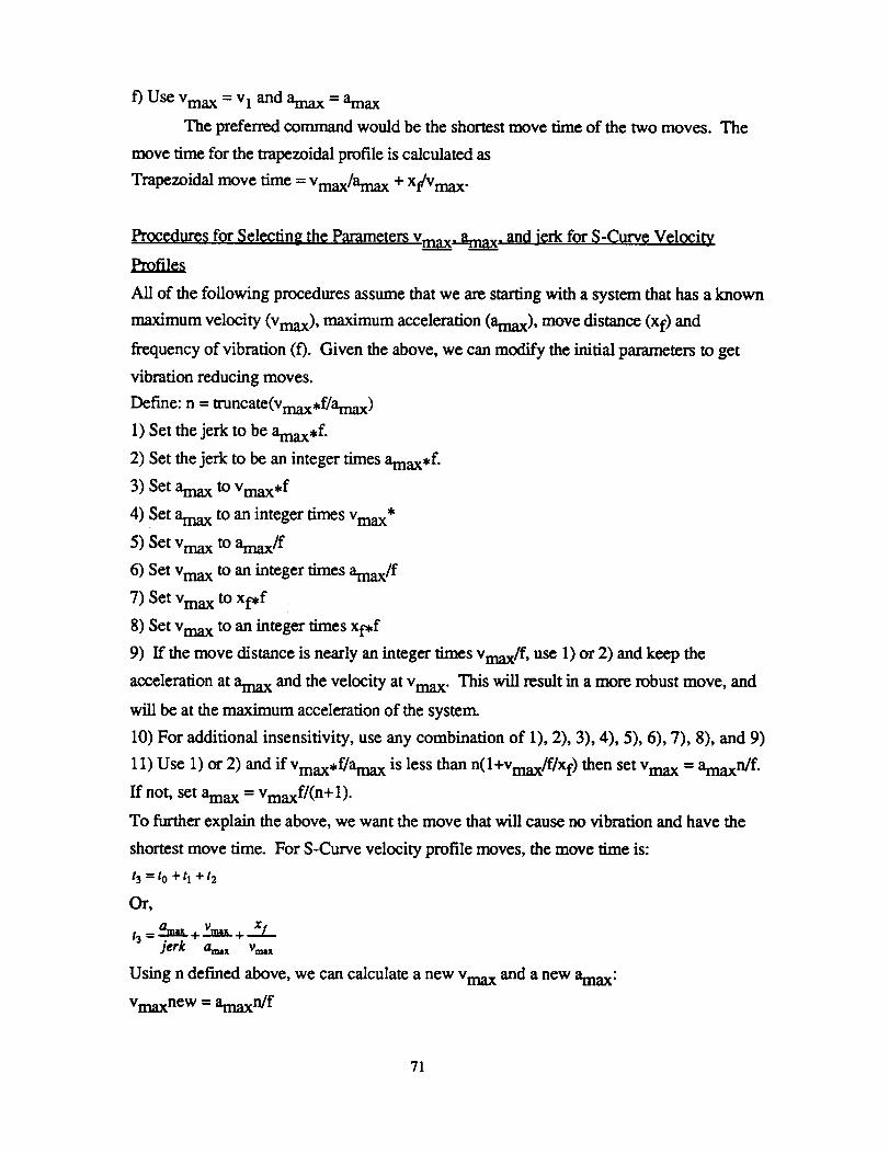
f) UseVmax - v! and ama x = ama x
The preferred command would be the shortest move time of the two moves. The
move time for the trapezoidal profile is calculated as
Trapezoidal move time = Vmax/ama x + xt/Vma x.
Procedures for Selecting the Paramcter_ Vm_m_m_m__max. and jerk for S-Curve Velocity
Profiles
All of the following procedures assume that we are starting with a system that has a known
maximum velocity (Vmax), maximum acceleration (amax), move distance (xf) and
frequency of vibration (f). Given the above, we can modify the initial parameters to get
vibration reducing moves.
Define: n = truncate(Vmax,f/amax)
1) Set the jerk to be amax,f.
2) Set the jerk to be an integer times amax,f.
3) Set area x to Vmax,f
4) Set ama x to an integer times Vmax*
5) Set Vma x to amax]f
6) Set Vma x to an integer times amax/f
7) Set Vma x to xf, f
8) Set Vma x to an integer times xf, f
9) If the move distance is nearly an integer times Vmax/f, use 1) or 2) and keep the
acceleration at ama x and the velocity at Vma x. This will result in a more robust move, and
will be at the maximum acceleration of the system.
10) For additional insensitivity, use any combination of 1), 2), 3), 4), 5), 6), 7), 8), and 9)
11) Use 1) or 2) and if Vmax,f/ama x is less than n(l+vmax/f/xf) then set Vmax = amaxn/f.
If not, set areax = Vmaxf/(n+l).
To further explain the above, we want the move that will cause no vibration and have the
shortest move time. For S-Curve velocity profile moves, the move time is:
t3 = to + tl + t2
Or,
t3 = a='_+Y-mL+--St--jerk at_x vrm _
Using n defined above, we can calculate a new Vma x and a new amax:
Vmaxnew = amaxn/f
71

amaxnew= Vmax,f/(n+1)
Calculatethenewmovetimes by replacing the velocity or the acceleration:
movetimevmax = amax/jerk + Vmaxnew/ama x + xf/Vmaxnew
movetimeamax = amaxXnew/jerk + Vmax/amaxnew + xidVma x
Select the shorter of the two movetimes and use the corresponding parameters. This will
result in an s-curve velocity profile that will be more insensitive to modeling errors, while
still maintaining a short move time.
Procedures for Selecting the Parameters Vm__0x_ma x. and Jerk for Parabolic Velocity_
Profiles
All of the following procedures assume that we are starting with a system that has a known
maximum velocity (Vmax), maximum acceleration (amax), move distance (xf) and
frequency of vibration (f). Given the above, we can modify the initial parameters to get
vibration reducing moves.
1) Set ml=intger value and set n l=integer value
2) Set ml=intger value and set n2=integer value
3) Set m2=intger value and set nl=integer value
4) Set m2--intger value and set n2=integer value
Input Shapers TM in Closed Loop Systems
For systems which are closed loops, an Input Shaper TM can be placed in the feed forward
branch of the closed loop, as shown in FIG. 76, in order to modify or eliminate unwanted
dynamics in the plant. Such a system is referred to as a shaper-in-the-loop (SIL) system
and conventional control system design techniques can be applied to the SIL system if we
consider the combination of the Input ShaperTM and the original (nominal) plant to
constitute a new plant, as indicated by the dashed line in FIG. 76, and then design the
controller with respect to the new plant. The new plant will have different magnitude and
phase characteristics that may need to be considered when choosing SIL closed loop gains.
Consider the following two cases.
Case 1: Shaped Frequency Greater than Closed Loop Bandwidth
If the shaped frequency is much greater than the nominal closed loop bandwidth, then there
will be little effect on the nominal gain and phase margins. Little or no adjustment of the
nominal gains will be required, and vibrations at the shaped frequency will be suppressed.
72

This techniqueis particularly valuablefor suppressingvibration frequenciesthat are in a
frequency band greater than the closed loop bandwidth and less than the Nyquist rate.
The shaper is tuned to the open loop vibration frequency to be suppressed. As the loop
gains are increased, the locations of the shaper zeros and the system poles at the vibration
frequency remain coincident.
The robustness property of the shaper improves under closed loop conditions. Poles
tend toward zeros as loop gains are increased, consequently any misalignment of the shaper
zeros with the poles at the vibration frequency is mitigated. Misalignment may be caused
by errors in vibration frequency estimation, or by poles that change location with system
configuration, with time, with payload, etc.
If the shaper zeros and poles at the vibration frequency are perfectly aligned, then little
additional robustness should occur as a result of feedback signals circulating through the
shaper. That is, disturbance rejection at the shaped frequency should not improve since the
design of the shaper prevents feedback signals from generating the control output at the
shaped frequency necessary to cancel the disturbance at the shaped frequency.
Case 2: Shaped Frequency within Closed Loop Bandwidth
If the shaped frequency is within or near the nominal closed loop bandwidth, then there
may be a significant effect on the nominal phase and gain margins, thus requiring
adjustment of the nominal gains (or modification of the filtering approach) in order to
obtain a stable system with good transient response. Vibration at the shaped frequency will
be suppressed, however, depending on the approach taken, the closed loop bandwidth may
be degraded relative to the nominal system bandwidth depending on the amount of phase
lag introduced by the shaper.
Therefore, for every closed loop system in which the input is shaped external to the
closed loop, there should be an equivalent SIL system in which the shaping occurs inside
the closed loop. Continuing along these lines, it is possible to make a SIL system
mathematically equivalent to a system with a preshaped input. Consider the SIL system of
FIG. 77, in which a shaper of transfer function S is inserted in the feed-forward branch of
the loop and the inverse shaper S- 1 is inserted in the feed-back branch. This system has
the same overall system transfer function as the system of FIG. 78 in which the shaping
occurs external to the closed loop. This is because the loop transfer function contains both
S and S- 1, which cancel each other, resulting in the original loop dynamics for signals
circulating in the loop; while reference inputs effectively pass through S only once. It is to
73

beunderstoodthat S is usedhereasa matterof convenienceandis not meantto imply a
specifictypeof transfer function. For example, in the case of digital systems, S may be the
ratio of two z-transform polynomials; while in the analog case, S may represent a Laplace
transform. Note that in an actual application using a digital controller, the cancellation
would be implemented in a control computer. Since the implemented filter and its inverse
are known exactly, the degree of cancellation depends only on the numeric precision of the
computer.
Insertion of the inverse filter in the feedback branch eliminates the phase and gain
modifications caused by the shaper inserted in the feed forward branch, effectively
converting the SIL system to a prefiltered system. Therefore, for this implementation, the
SIL filter is tuned to the closed loop vibration frequency to be cancelled.
Other filters besides S- 1 may be inserted into the feedback path to partially (instead of
totally) eliminate the phase and gain effects of the feed forward SIL filter. For example the
filter [(1-ot)+ctS- 1], where 0<ix<l, can be inserted in the feedback branch. At ix=l, the
phase and gain effects of the feed forward SIL filter are completely eliminated, and the
system behaves as in FIG. 77, or equivalently FIG. 78. At tx=0, the system behaves as in
FIG. 76 and the phase and gain effects of the feed forward SIL filter are unaltered. Thus,
varying tx from 0 to 1 effectively continuously varies the filter action from inside the loop
to outside the loop.
Phase and gain effects due to a SIL filter inserted in the feed forward path can also be
modified by modifying the SIL filter itself. Shorter length filters have decreased phase lag
and gains that tend to increase with frequency. The shortest filters have negative going
pulses that can approximate derivative action. Using a short length SIL filter may allow
compensation of both the phase and gain curves resulting in increased bandwidth.
Miscellaneous Shaping Applications
The technology has been discussed primarily in the context of controlling the motion of a
mechanical system, in general, and of a robotic arm with one or two modes of vibration, in
particular. However, it should be understood that the technology is not restricted to these
cases. It is also applicable to other types of dynamic systems, including electrical and
chemical systems and to systems with more than two modes of vibration.
For example, to control the altitude of weather balloons, ballast is released to gain
altitude and gas is vented to lower altitude. When altitude changes are made in this manner,
the balloon will usually oscillate about the new altitude with a predictable frequency. The
74

altitude control effort can bc shaped to greatly reduce oscillations in altitude. For example,
a release of 10 lbs. of ballast shaped by a ZVD shaper would result in the dropping of 2.5
lbs. initially, then 5 lbs. after one half period of the vibration, and finally, the remaining
2.5 lbs. would be dropped after one period of vibration.
Finally, although the above examples have utilized impulse sequences, it should be
understood that sequences of finite duration pulses may be used instead. The pulses or
impulses can be constrained to begin and/or end at specified intervals, as is the case with
impulses designed for use with systems which are discretized in time, and they may also be
constrained to have specified amplitudes. In addition, pulses may be fixed in amplitude but
variable in duration or fixed in duration but variable in amplitude.
FIG. 79 illustrates a standard implementation of the technology. An input is shaped
using one of the methods described previously and the shaped input is used to drive the
dynamic system. Shaping the input comprises convolving the input with a series of
impulse sequences, or equivalently, as shown in FIG. 79, delaying and scaling the input
by various time delays and gain factors and then summing the delayed and scaled inputs to
form the shapedinput. Different impulses sequences may be used, as disclosed herein, to
achieve different characteristics for the shaped input or for the response of the dynamic
system.
75

Figures
2.0
1.5
1.0
0.5
0 I0 5 10 15 20
System Input Impulse Sequence
\f
2.0
1.5
1.0
0.5
00
Shaped Input
....... A! Component
omponent
/ ':xL1-_,_\
/ , ,I I "-.
5 10 15 20
Shaped Input
Figure 1 a, b, c: Convolution of a System Input with anImpulse Sequence Produces a Shaped Input
°,=_
<
ml
A2
T2 Time
Impulse Sequence
<==_=-%"-A!01 --0
Vector Diagram
Figure 2 a, b: An Impulse Sequence and its Corresponding Vector Diagram
77
_lliD_t_ _A_ eta_ ttotr
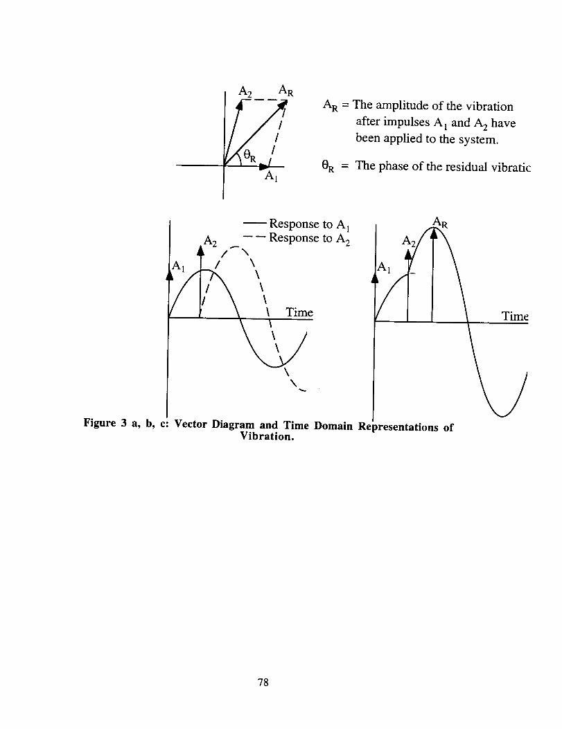
A 2 AR
f/"-11
A R - The amplitude of the vibration
after impulses A 1 and A 2 have
been applied to the system.
OR = The phase of the residual vibratic
A1
Response to A l
A2 -- -- Response to A 2/ \
/ \
i _ \\\ Time
N
Figure 3 a, b, c: Vector Diagram and Time Domain RepresentationsVibration.
of
78
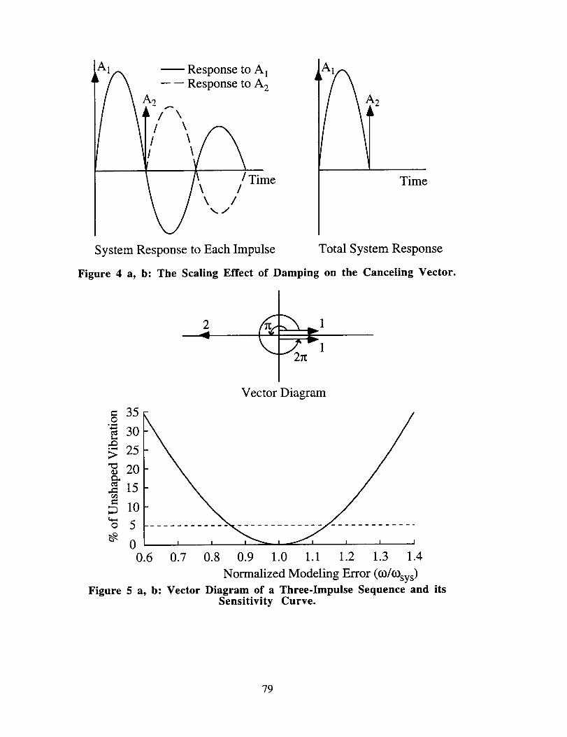
Response to A]
-- -- Response to A 2
k2
/ \
// \
Time
\ /\ /
_J
_2
Time
System Response to Each Impulse Total System Response
Figure 4 a, b: The Scaling Effect of Damping on the Canceling Vector.
2
= 35O
o ¢,,,_
30,.Q, ,w,,_
> 25
"_ 20
= 15
O
Vector Diagram
10
5
00.6
i ............
0.7 0.8 0.9 1.0 1.1 1.2 1.3 1.4
Normalized Modeling Error (o3/COsys)Figure 5 a, b: Vector Diagram of a Three-Impulse Sequence and its
Sensitivity Curve.
79
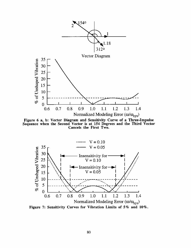
3530
20._ 15
o 5
0
2_54 °
_1.18
312 °
Vector Diagram
0.6 0.7 0.8 0.9 1.0 1.1 1.2 1.3 1.4
Normalized Modeling Error (o3/COsys)Figure 6 a, b: Vector Diagram and Sensitivity Curve of a Three-Impulse
Sequence when the Second Vector is at 154 Degrees and the Third VectorCancels the First Two.
........ V= 0.10
= 35 V = 0.05O
'_ 30 /,-, \ I_ Insensitivity for _1
25 :.._ I V = 0.10 I //"_ 20 "' I I ."""-Nk I I._---Insensitivity for--_l I /."/'_ 15 '...'_ I V = 0.05 I i/.."
10 ..... - ...... -..--.... --.:....... !"%, oO" "" ''-. ."
_" 0 I "1,," "'-," , '
0.6 0.7 0.8 0.9 1.0 1.1 1.2 1.3 1.4
Normalized Modeling Error (o_/O_sys)Figure 7: Sensitivity Curves for Vibration Limits of 5% and 10%.
80

1.2
mM
o_
0.8
0.6 •
0.4
o°°°"
0.2
0.00.0
Response to step input
......... Response to shaped input
I I I I I I
0.5 1.0 1.5 2.0 2.5 3.0
Time (see)
Figure 8: System Response to a Step Input and a Shaped Input
= 35O
o_,,q
_ 30
°w,,_
> 25
_ 20
.= 15
_ 10
o 5
_ 0
0.6
Figure 9:
<_ _ Experim. ental ,"
•......., ._ Theoretical ,," ,
o II'...\ o°
",b mB
Q_, e J, •
0.7 0.8 0.9 1.0 1.1 1.2 1.3 1.4
Normalized Modeling Error (m/_sys)Experimentally Determined Sensitivity Curve for V=0.05.
81

= 35O
.¢.._,4,..I 30
> 25
_ 20
.= 15
_ 10
o 5
00.6
Experimental........ Theoretical
-..,,,.,,,,,.,,,,,. .'"'"'................ ,..........////"
0.7 0.8 0.9 1.0 1.1 1.2 1.3 1.4
Normalized Modeling Error (co/O_sys)Figure 10: Experimentally Determined Sensitivity Curve for V=0.10.
q_
,4111
t..
O*lid
25 -
20
15
10
5
00.60 0.80 1.0 1.2 1.4
Normalized Frequency (co/03sys)
Figure 11: Sensitivity Curve for the Four-Impulse Extra-Insensitive Shaper
82

A_
0.8
0.7
0.6
0.5
0.4
0.3
0.2
0.1
Increasing 4
4= 0.3
I I I
0.0 0.20 0.40 0.60 0.80 1.0
Figure 12:A1 for the SI Shaper as a Function of I and 4.
A_
0.6
0.55
0.5
0.45
0.4
0.35
0.3
0.25
Increasing
= I I I I
0.0 0.20 0.40 0.60 0.80 1.0
Figure 13:T2 for SI Shaper as a Function of I and 4.
83
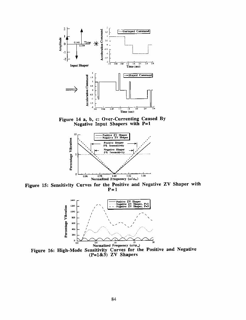
"0e_E<
-1
-2
2
i +O.t,m Time __ _ o_
_ 0.194 ._ I}
41.5
Input Shaper
I ..... Unshaped Command I
qJ
i i i 714oo 040 080 LI2 I./ 2.o - 2!8
Time (sec)
2
e_ 1.5
1
i 0.5
_ 41.5-1
_ -I.5
-7.0.11
haped
Time (see)
Command[
2.4 2.X
Figure 14 a, b, c: Over-Currenting Caused ByNegative Input Shapers with P=I
t0
O
5
eL
-- --Positive ZV Shaper I
• [ ..... Negative ZV Shaper I ,''
• _ _ Positive Shaper _l ," _,
_,• 1_ 5% Insensitivity -- --I "''/
_',_ _ Negative Shaper _ _" /
_ "_',/ 5% Insensitivity _'[,/
0.96 o.98 t.oo t.o2 1.o4Normalized Frequency ((D/COrn)
Figure 15: Sensitivity Curves for the Positive and Negative ZV Shaper withP=I
14_X) --
g_ L2(K) --
._
LIXX) --t-
_,. _o -
(3(11 __
2(11
[1
--Positive ZV Shaper I
f ,_ ......... Negative ZV Shaper, P=I
/ \ - - -Negative ZV Shaper, P=3
/ \
/ \ /_N.
l \ / \
/ \ /
/ /"'-... ,," . '. . ..[
- -.."
0.0 5.11 I0 15 20
Normalized Frequency (co/¢o_)
Figure 16: High-Mode Sensitivity Curves for the Positive and Negative(P=I&3) ZV Shapers
84

20 .... Negative ZV Shaper I /
j--Negative ZVD SHaper[ /
,_ k ____. ZvDSha_er /____ /\ l- ,s. I.,e.,i,ivity -I /
_\ / .,'shaper,/ /
I) I I I I I I I I ' '-""'_ t .--._', , I .... I , I
0.8 0.9 1.0 I. 1 1.2
Normalized Frequency (&co_)
Figure 17: Sensitivity Curves for the NegativeZV and ZVD Shapers with P=I
70 --
@
I,
I., _ 55
_ Q
40
1.0
I I I [ I
q
2.0 3.0 4.0 5.0 6.0
P
Figure 18: Length of Negative ZVD Shaper, z=0
2O
"_ 15
(1
..... Negative ZV Shaper I /
-- Negative ZVD Shaper I /
[ ..... Negative E! ShIper I /:/
aI ,"\ '.. , //s' ,.'
G _, a
... ...........N% o 4 e " .."
..... "';.A/' ,,'_w..._'_t"J, /"./. , . I , i
0.8 0.9 1.0 1.1 1.2
Normalized Frequency (co/co,.)
Figure 19: Sensitivity Curves for the NegativeZV, ZVD, and EI Shapers with P=I
IO_) -- --Negative ZVD Shaper[
_ ..... Negative E1 Shaper I
2()0
0 b I "o.o 5o .J _5 2o
Normalized Frequency (¢_/co_)
Figure 20: High-Mode Sensitivity Curves for the Negative ZVD and theV=5% EI Shapers
85

81_)
O 7(X)
6(X)t-,
5111
_ 4_KI
2IX)
_., im
o
I--Negative El Shaper
-- I ..... Negative El Shaper with|
-- I 7 Hz Vibration LimiUng I /
_ /'.,i . o _
_J t
%, # % at 7 Hz"_J 1 , I , [ _ I , I
I).0 2.0 4.0 b 0 H.I) 10
Normalized Frequency ((O/C0m)
Figure 21: Effect of 7 Hz Vibration Limiting
5(X} --
ee0
4_X}
eun
_K) High-Frequency
,,2Ill}
e_
(I I i Io.,) 2.o 4.o 6_. _.o u_
Normalized Frequency (_/m_)
Figure 22: Sensitivity Curve for the EI Shaperwith Low-Pass Filter
[,2 B
[
i o.a- /,,'/
/ , ° ._J ",J --
06 -- /,:I[ I-----Unshaped Response I• J[i [ .... Negative ZV Shaper I
0,4 -- J,_/' I -- - "Negative ZVD Shaper I/_--Negative E1 Shaper I
0.2 --[/
0 I/i T, I,_,,1_ _, , I , , , , f, , , ,I .... I
0.00 0.50 1.00 1.50 2.00 2.50 3.00
Time (sec)
Figure 23: Plots of Unshaped and Shaped Responses
1.05
f ; ,"°'".,
¢II / "" , '
_O 0.9 _ ': -"'",-- Negative ZV Shaper |i / - - .N,,_,_zvps_: .... II ..' _N_gali, v--s_ E, ShaperI
Time (sec)
Figure 24: Zoom in on Residual Vibration When Frequency is 25% Lowerthan Modeled
86

[____ 1 x 2
Q Off f ff f f ff f f_J'f f ffJ f ff f fief
Figure 25: Simple System Model
1.02
0.50 I0 5 10 -z -2
System Input Impulse Sequence
1.0
0.5
Shaped Input 0
-0.5
-1.0
10
Figure 26 a, b, c: The Shaping Process for CreatingConstant-Magnitude Pulses
87
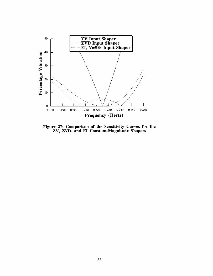
so - --ZV Input Shaper..... ZVD Input Shaper
......... EI, V=5% Input Shaper
g_ 40 --
..
30
_" /
\ ,'/'
20 /.-. -,..-.\ 2'
_'_ """-i \ ,./.,"10
o I "1''_ ........................ _".i'"" I I
0.180 0.190 0.200 0.210 0.220 0.230 0.240 0.250 0.260
Frequency (Hertz)
Figure 27: Comparison of the Sensitivity Curves for theZV, ZVD, and EI Constant-Magnitude Shapers
88

0.8
0.6e_
o_
o0.4
0.2
00.0
L
-._: .::->- ....._- : :T"-.- 0.1_1 -_. ..... .i=
• r_#g' ZVD, k = 1.0
I ZVD, k = 0.9ZVD, k = 0.8
ZVD, k = 0.7
I I I2.0 40 6.0 s.o lo 12
Time (sec)
1
0.8
0.6
0.4
0.2
00.0
f"
/ i--........ EI, k = I.t I _l,k -- o. °
:" I ..... Ei, k :0."Lz" [--ELk= 0.787' I I I I I
2.0 4.0 6.0 S.0 10 12
Time (see)
Figure 28 a, b: Comparison of Responses to ZVDand EI Shapers for Various Values of k
89

120 -
I00
80
e_
60
40
m
B
m
2°L/ o ,0.00 2.00 4.00 6.00 8.00 10.0
Frequency (Hz)
Figure 29: Frequency Spectrum of Unshaped Vibration
80OO
7000 • •m• n me
6000
5000
4000
f/'2000 ' ..... Shaped Res ons
1ooo
== o i_-II i i i i I l i0.0 0.20 0.40 0.60 0.80 1.0 1.2 1.4 1.6
Time (sec)
Figure 30: Comparison of Unshaped and Shaped Responses
90

8 $2-8S+31
16 S 22S-1
l 4_ $2
0 At
S = sin
8S 2 1
T 25116i24S2
7_.At 3At 4At Time
°_1 2r_r= -- At=
o_2_ e I + co2
Figure 31: Two-Mode, Symmetric Sequence.
3o
•-_ 20
-_ 15
"_ 5
o0.50 1.0 1.5 2.0 2.5 3.0
System Frequency (Hz)
Figure 32: Insensitivity of Five-Impulse Sequence for 1.0 and 2.25 Hz.
91

. | " ,.
Figure 33: The Proconics CMS.
I 15 impulse sequence I9 impulse sequence
........ 2' ......"1
-" 5
04 6 8 10 12 14
Frequency (Hertz)
Figure 34: Insensntivity of 9 and 15 Impulse Sequences.
92

A
p,
200400
20020"10
o 20000e.,
IJJ
19980 ....................C0
,m
•_ 1996Oo 0.0 0.5
a.
J Command Position I
- .......J.............J.............i.............i............i.......
.0 1.5 2.0 2.5 3.(
Time (sec)
Figure 35: Encoder Position for R-Axis Slew. (detail)
a)
40
_, 3020
"_ 10
0t, -lO
¢, -20
-3O
I I
iiiiiiiiiiiiiii0.0 1.0 2.0 3.0 4.0 5.0
Time (sec)Original Response-No Shaping, Slow S )eed.
20 - ..........................i...............i................i..........
0 :=._.............. : . _.. i..
t, -lO - ..........J -2o - ..........
-30 '"0.0 1.0 2.0 3.0 4.0 5.0
Time (sec)
b) Unshaped Response-Fast Speed.
93

4O
10 ..........i................_..............._................i..........
_I, -20
-300.0 1.0 2.0 3.0 4.0 5.0
Time {sec !
c) Shaped Response-Fast Speed, 9-Impulse Sequence.
4o
_, 302o
"_ 10._
I
............................!..........................................._---
=.
-lo ............................................J................J..........--, -_o:-=-..........,................................i..........................4
-3o - I I I "0.0 1.0 2.0 3.0 4.0 5.0
Time {sec)
c) Shaped Response-Fast Speed, 15-Impulse Sequence.
Figure 36: Unshaped and Shaped Response.+16.78 in. R-Axis Moves.
Retro Mounted on Side of Gripper.
94

-- Unshaped Slow I15 Impulse Shaped, Fast
1.000========================================::::::::::::::::::::::::::--!!!i!!i!!i!!!!!!!i!!!!i!!!!!!i!!i!.,=-!i_!!!!!!!!!!!!i!E!!!:,i!!!D"
= O.lOO .-::!::::,_,i,,.--_:i:'i,_::::i::_::_::_
E- 0.010
0.0011 0
Freq (hz)
Figure 37: FFT Magnitude Comparison.+16.78 in. R-Axis Move
Retro Mounted on Side of Gripper.
Figure 38: A Three-Impulse Sequence May Not Fit the DigitalTime Spacing of the System
._ 20.00 r-- .......................:............................_.................... •E, i i GAMS Sequence I17 50 _-_: ....................i............................i................... ---El---Three Impulse Sequence I
._ =," _ _', i i ..... Linear Extrapolation SequenCe
__.oo_:_,_........i............................!..................._ Murph,,W.,,n.eSequence,'.12.50 _-:":'"_',-:i .......................Besired---Frequenc_y ..........i/ ...............i: '''-_ ..........!
¢_ E " "_,i, i 2.88 Hz_. !/ . !" i10.00 :-':.......................i............................i..........................: ...............:..........,_...........................i
_oo__........_i;r_:_i ..............::i=_............i..........................._:; ........"= ....rr: ;_: Irr2_ r/::i_" 0.00 " " "
2.00 2.25 2.50 2.75 3.00 3.25 3.50
System Frequency (Hz.)
95

Figure 39: Comparison of Sequence Digitizing Methods.
fvibration = 2.88 Hz., _ = 0.00, fsample = 10.0 Hz.
Three Impulse SequenceMatrix Inversion Sequence
Figure 40 a, b: Three Impulse Sequence and Sequence Found By Matrix
Inversion for fvibration = 2.88 Hz., _ = 0.00, fsample = 10.0 Hz.
Figure 41:
Motor &
O_ Thin, FlexibleBe_
0 ]1-_ Laser tor
Flexible Beam_,. o 0 J RetroReflec
Rotary Table E[_ Laser
l[ Interferometer
Experimental Set Up for Tests on the Rotary TableWith Two Modes of Vibration.
,_,.0.90
"-'0.70
t-o
*_
"" 0.50
oe_
cO.30.Q
I_ 0.10
-0.100.00
=================================......................on....o. o,.o,4___........_..._::.,....i .............l ............. Unshaped Encode l__ ............_....ii[]............[ _ Shaped Setpoint I
iiiiiiii i_! )i!_iiii_illl []..... ..... Shaped Encoder |
0.25 0.50 0.75 1.00 1.25 1.50
Time (see)
96

Figure 42: Position Set Point and Encoder Position for Shaped andUnshaped Maneuvers.
1.00 -------_ _-....... :,...... l!! Unshapede: 0.60 ...............................!_.... "............. Nine-Impulse Sequencel
':! ......_ ..... 2@Five Impulse Sequencl_/
0.60 .................................:ii-_........................................................................................:=- i_,
0.40 ....................................:.£.i......................................................................................a.
0.20
•J 0.00
-0.200.00 0.50 1.00 1.50 2.00 2.50 3.00
Time (sec)
Figure 43: Laser Position of Unshaped and Shaped Maneuvers.
0.150
_, 0.100
_" 0.050
0.000
"_.-0.050
,..-0.100
,_-o.15o,,.J
-0.200
-0.2500.00
iiiiiiiiiiiiiiiiiiiii-iiiiiiiiii iii1 ,.............. Nine-Impulse Sequence /
---_.. 2@Five Impulse sequencIp|
I I I I I
0.50 1.00 1.50 2.00 2.50 3.00
Time (sec)
Figure 44: Residual Vibration of Unshaped and Shaped Maneuvers.
97

A
,,: 0.004
0.002
0.000el
-0.002
'_-0.004
-0.0061.00
0.006 ............................................................................................................................
............................... J Nine-Impulse Sequence /.............. 2@Five-lmpulse Sequencls
.......... "" ..................... _"....................!.....................i..........................................!
................ i"
i F
I I I1.50 2.00 2.50 3.00 3.50 4.00
Time (sec)
Figure 45: Close-Up of Shaped Residual Vibration.
98

o o +
+++.by ky
M
Your
L__ Xout
Figure 46: Two-Mode Model of a Flexible System Under PD Control.
-0.2
O_ -0.4"_,
Ogh --0.6
-0.8
-1
I
.0.6 0.6
...p.oI I I I I
-0.4 -0.2 0 0.2 0.4
X Position
Figure 47: Comparison of ZVD Shaped and Unshaped Responses to a Unit-Circle Input (fl=f2=l Hz, z1=z2=0.05, Unshaped Command Length=10
sec.).
-i
.m
_. 0.5
o
cell
-o.5
r_ -10
-- Unshaped X Command-- •Unshaped Y Command
__ I--a-Shaped X Command
[--4 .Shaped Y Command
2 4 6 8 10Time (see)
Figure 48: Unshaped and ZVD Shaped Command.
99

0.2
e_o 0.15
[.rd 0.1
005m_e
_\ _ I -- Unshaped, ¢--0
i \_ -- -Unshaped, ¢--0.05
_,\'_ I ..... Unshaped, _--0.I, \ _'_ +Shaped, _--0
/ \,, \
_'"2--_ _.._ ._ _,._ ....
5 )0 15 20 25 30
Vibration Cycles/Circle
Figure 49: Unshaped and ZVD Shaped Radius Envelopes (r =1).Shaped Curves are Essentially the Same.
Note: All
0.12
_" O. lo_J_. 0.08
_.l 0.O6
I).04
0.02m
- - - Unshaped, r=l.5
-- Unshaped, r=l.3
i-! ZVD Shaped, r=-l.5 [
ZVD Shaped, r=l.3 I
Shaped-_: _ _ _ ---a-=- _ :.
- 0 -40 40 80
Departure Angle Relative to +X Direction
Figure 50: Radius Envelope as a Function of Departure Angle forCycles/Circle= 11.
0.14
_a 0.12
O
0.1
0.08
0.06
.._'_ 0.O4
_x,-- - Unshaped I..... ZVD Shaped I
--El Shaped I
ee 0.02 ":_ .. . ..
0016 _ ,• 0.7 0.8 0.9 1.0 l. i 1.2 1.3 1.4
Frequency (Hz)
Figure 51: Response Radius Envelope as System Frequency Varies (InputsWere Designed for fl=l Hz, r=l, Zl=Z2=0, and Cycles/Circle=ll).
E
1 ...... _F ....... :-- -. ' _...i ......... i!
................ !......!p
ii
.........._ i _ _ _ ._._j .......":
o 0.6
oeL
0.4
0.2
0
-0.2 I t
-0,2 0,0 0.2 0.4
I I I I I
0.6 0.8 1.0 1.2
X Position
100

Figure 52: Comparison of ZVD Shaped and Unshaped Responses to a Unit-Square Input (r =1.5, zl=z2=0.05, Cycles/Square=15).
1.4 - --Unshaped X Input --,,-Shaped X Input I
'_ 1.2 -- -Unshaped Y Input ---* -Shaped Y InputI•-, : :
.< 0.g
= o.6 i /? i\\o ,.,._ O.4
° , ,%\ ,,_ °.2 Z, ___/ _ j\,._2 4 6 10 12 14 16
Time (sec.)
Figure 53: Unshaped and ZVD Shaped Commands for a Square Trajectory.
t., 0.05 --
0.03 i_x
0.01
10.0
--Unshaped, _:_| --4t-Shaped, _=0 I---Unshaped, _=0.1 -e- -Shaped, _=0.1 I---O--Unshaped, _=0.3 --_"-Shaped, _=0.3 I
20.0 30.0 4o.0 50.0
Cycles/Square
Figure 54: ZVD Shaped, EI Shaped, and UnshapedFunction of Cycles/Square and z. (r =1.5).
Mean Error as a
1.4 .......- .........=........'........-"-'_F ........_........_.........;:
o= 0.8 -"_" __ ......... i
0.6 ......._., -;iCh
;_ 0.4
0.2 ....... _......... ; ......... _......... i
0 ........... i
-o.2 I I I I i i I i-0.6 -0.4 -0.2 0.0 0.2 0.4 0.6 0.8 1.0
X Position
Figure 55: Unshaped and ZVD Shaped Responses to a Unit-Square Input
with a Departure Angle of 30 ° Relative to the Low Mode (r =1.5,zl-z2=0.05, Cycles/Square=15).

Im
Figure 56:
0.035
0.03 _nshape_0.025 "_._..._"/ I _/
0.02 _ - - _
--Unshaped, r=l.$]
0.015 - - Unshaped, r=i.3]
_ Shaped, r=l.S ]
0.01 -@ Shaped, r=l.3 |
0.005 Shaped
I I
Departure Angle Relative to X Direction
Error Mean as a Function of Departure Angle forCycles/Square=17.
0"06 t I1 t_tx [_ - -Unshaped Mean ]1
0.05 I i _ ] ..... ZVD Shaped Mean|It I I I _--EI Shaped Mean
0.04 _ II J l I e_
0.03 I I II I / N| f I I I-- l I _I
| I I I iI I
_" 0.02 '" I I _ iV. | I l I l I
.... _ ||I I l l I I i l
0 I _ i'_-'-T'" _ I _'"1 I'''_ I
0.6 0.7 0.8 0.9 1.0 1.1 1.2 1.3 1.4Frequency (Hz)
Figure 57: Mean of Square Tracking Error as System Frequency Varies(Inputs Were Designed for fl--1 Hz, r=l, zl=z2=0, and
Cycles/Square=15).
-0.2
om -0.4
eL
_, -0.6
-0.8
-1
I I I I I
-0.60 -0.40 -0.20 0.0 0.20 0.40
X Position
I
0.60
Figure 58: A Circular Response From Shaping a Larger than DesiredRadius and Allowing for Transients (r= 1, zl= z2= 0, Cycles/Square= 8).
102

. o.oo2 Side 1 I Side
0.001
0.0005
o 5
I Side 3
tt10 15
Time (sec.)
Side 4
2O
Figure 59: Shaped Square Tracking Error for r=l.5, Zl=Z2= 0,
Cycles/Square=15, and Departure Angle = 30 o.
/Recording /
Surface
X
Y
Figure 60: Experimental Setup
103

Figure 61: Unshaped 3x3 in. Square Trajectory
Figure 62: EI Shaped 3x3 in. Square Trajectory
104

Figure 63: Unshaped 3x3 in. Square Trajectory with Added Endpoint Mass
Figure 64: EI Shaped 3x3 in. Square Trajectory with Added Endpoint Mass
105

12 [ Unshaped I10 .-" ...... Shaped
.,_ 8.0
6.0 ."
,/
_ 2.0 '"r,,)
o.o !: :!:. !0.00 0.25 0 50 0 .... I. 5
me
Figure 65: Shaped and Unshaped Trapezoidal Velocity Profiles.10 rad. Slew, Shaping Sequence for 3.8 Hz. and 8.2 Hz., No Damping.
O --
"4
<-
/
I
I_
Q n
° 7L<
i .......
I I I I I I
Time Time
Figure 66 a, b: Superposition of Four Shaped Acceleration StepsYields a Shaped Trapezoidal Velocity Profile
106

O
_J
O
[-
_ou
Vmax
amax
100
80
60
4O
20
0 I I I I I0 10oo 2000 3000 4000 5000
Step Rate, Full Steps/Sec.
Figure 67: Pullout Torque-Speed Curve for a Stepper Motor.
___L_
I
tl Time
= Vmax/ama x
I
t2 t3
= xf[Vma X
TimeI
I
---1--|
Figure 68 a, b: Trapezoidal Velocity Profile and Its CorrespondingAcceleration Profile
107

amax
Time
amax I
= xf/Vmax
I Time lI
-1-
I
amax _ tl= Vmax/ama x
I 1 Time
, II_k
Figure 69 a,b,c,d: Convolution of a Step in Acceleration with Two Two-Impulse Shapers Yields the Acceleration Profile for a Trapezoidal Velocity
Profile.
40
35
30
_ 25
eL 20
o_ 15
L.
_ 10
f _t, _ Case I:
v ._ =2
I a =2
xt=6
mt=l
_ m 2=3
0.960
!
-- -- - Case 1: !
v =2 I
amz=l Ix =6 I
g Im =2
t I III / /
m2--3 /
0.980 1.00 1.02 1.04
Frequency (Hertz)
Figure 70: Insensitivity Degrades When ml is Increased.
108

I...
oo_
elL,
40
35
3O
25
20
15
10
5
0
I/.• " _mz--3 I : .
• "°. _ ..... 1112:=-1 ,_t- ', ...... - ,'i ..", "...,...,, ,'/...'/
,,,',..../N..:..'., ,',:../
_- x,:._,..: ,,/;;./I \'._". "-" /
• • .._ I,/."
0.960 0.980 | .130 1.02 1.04
Frequency (Hertz)
Figure 71: Insensitivity Degrades When m2 is Increased.
109
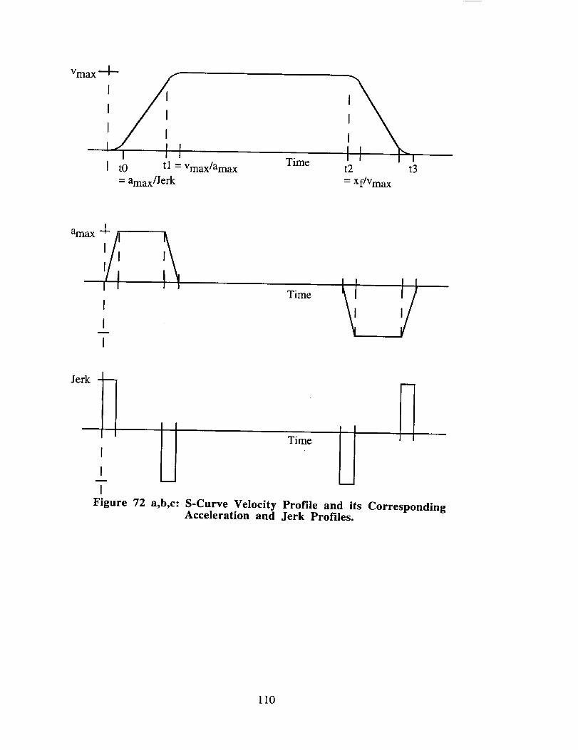
Vma x --]--
I
I
i tO tl = Vmax/amax
= amax/Jerk
TimeI
t2 t3
-" X f/Vma X
ama x --1-
I
I
I
Time
I
I
i
U Time
Figure 72 a,b,c: S-Curve Velocity Profile and its CorrespondingAcceleration and Jerk Profiles.
110

Jerk
Time
erkI to
I
I
Time
Jerk I ]
I
I
I
tl
Time
Jerk
I
I
!
I It2
TimeI I I
Jerk
tl
__1I
Time
t2
IIFigure 73 a,b,c,d,e: The Jerk Profile for the S-Curve Velocity Profile is
Composed of a Step in Jerk Convolved with Three Two-Impulse Shapers.
111
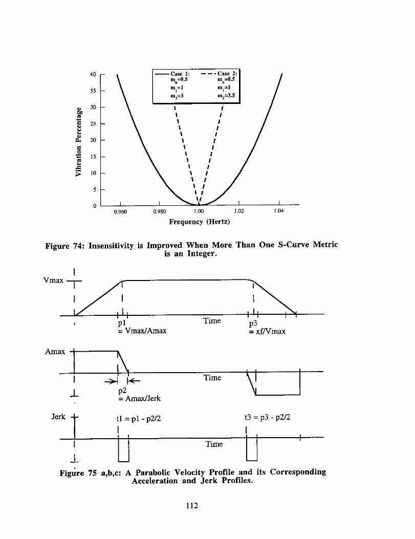
G
t..
@.m
t-
40
35
30
25 -
20 -
15 -
10 -
5 -
0
t l--Case 1: -----Case 2:l /\ I m°=0"5 m°--0"5I /\ I ml=l m'=t I /
[ m2=3 mz=3.5 [ /
\ ', / /\ ', / /
', / /
', / /
0.960 0.980 1.00 1.02 1.04
Frequency (Hertz)
Figure 74: Insensitivity is Improved When More Than One S-Curve Metricis an Integer.
IVmax
, p 1 Time p3= Vmax/Amax - xf/Vmax
.j_ p2= Amax/Jerk
Time
Jerk -_- t I = p 1 - p2/2 t3 = p3 - p2/2
! I I
I U Time U II__
Figure 75 a,b,c: A Parabolic Velocity Profile and its CorrespondingAcceleration and Jerk Profiles.
112
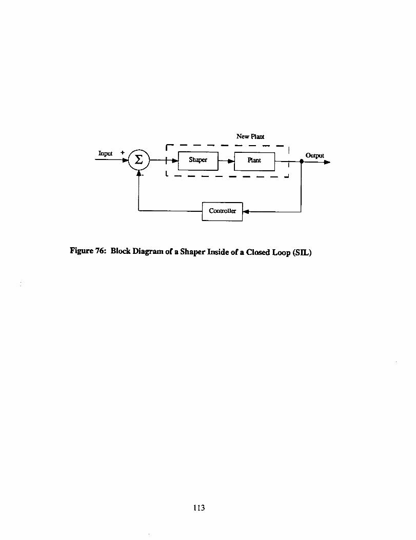
Input
New Plant
, I
I 'I. .j
ControUe_ I-_
OutputL L_• v
Figure 76: Block Diagram of a Shaper Inside of a Closed Loop (SIL)
113
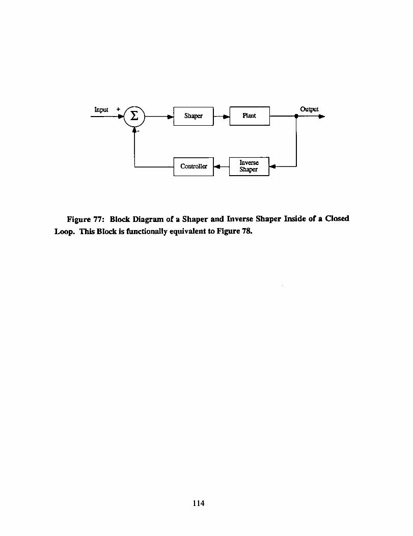
Input
H OutputShaper Plant _
Ico_o__ _= _-
Figure 77: Block Diagram of a Shaper and Inverse Shaper Inside of a Closed
Loop. This Block is functionally equivalent to Figure 78.
114

_p°t s_ I_ :_ I_t I
OutputV
Figure 78: Block Diagram of a Conventional Shaped System.
115

GAMS Input Shaping TM Scripts
William SinghoseConvolve, Inc.
© 1993-95 All rights reserved.

GAMS Input Shaping TM Scripts
Contents
I. Introduction ...................................................................................... 1
Road Map to Scripts ...................................................................... 1Overview of Script Structure ............................................................ 1GAMS Formatting Conventions ........................................................ 1Running GAMS ........................................................................... 2
Procedure for Digital Scripts ............................................................ 21I. Generic Input Shapers ......................................................................... 4
ZV shapers ................................................................................. 4ZVD shapers ............................................................................... 4EI Shapers ................................................................................. 4Multiple-Hump EI Shapers .............................................................. 4SI Shapers ................................................................................. 4Frequency Sampled Shapers ............................................................ 5Least Squares Shapers ................................................................... 5
III. Negative Input Shapers ....................................................................... 5Negative ZV shapers ..................................................................... 5Negative ZVD shapers ................................................................... 5Negative EI Shapers ...................................................................... 5Negative Multiple-Hump EI Shapers ................................................... 5Negative SI Shapers ...................................................................... 6
IV. Constant-Amplitude Pulse Shapers ......................................................... 6CAP ZV shapers .......................................................................... 6
CAP ZVD shapers ........................................................................ 6CAP EI Shapers ........................................................................... 6CAP Multiple-Hump EI Shapers ........................................................ 7
References .......................................................................................... 7
Appendix A - Hard Copies of GAMS Scripts .................................................. 8Generic Input Shapers .................................................................... 8
ZV-DIG.grns ..................................................................... 82-DIG.gms ....................................................................... 9EI.gms ............................................................................ 10EI-DIG.gms ...................................................................... 12SIOHUMP.gms .................................................................. 14SI 1HUMP.gins .................................................................. 17IMP23TR.grns ................................................................... 21HUMP01TR.gms ................................................................ 23FS.gms ............................................................................ 25LP-2MOD.gms ................................................................... 27
Negative Input Shapers .................................................................. 30NEGZV.gms ..................................................................... 30NEGZVD.gms ................................................................... 31NEGEI.gms ...................................................................... 32
Constant-Magnitude Shapers ............................................................ 35CAPZV.gms ...................................................................... 35CVCAPZV.gms .................................................................. 36CAPEI.gms ....................................................................... 37

GAMS Input ShapingTM Scripts
I. Introduction
GAMS (General Algebraic Modeling System) is a linear and nonlinear optimizationprogram. The program is driven by user-generated scripts that describe the optimizationproblem. The scripts contain the constraint equations that are to be satisfied, the function tobe minimized or maximized, resolution criteria, and input/output commands.
This manual describes GAMS scripts that were written to design input shapers. There
are a large variety of scripts, each written to meet a distinct set of constraint equations. Tohelp the user locate and run the appropriate script, this introduction will provide a road mapfor locating a script for the system under consideration. The procedure for running GAMSwill then be reviewed.
Road Map to ScriptsThe listing and description of scripts is broken down into the following subheadings:
• Generic Input Shapers.
These shaper are used for the majority of applications. They are used on systemswith no special actuator limitations or abilities. If nothing is know about the systemexcept its frequencies and damping ratios, then these are the shapers to be used.
These scripts will solve for ZV[3], ZVD[3], EI[7, 9], SI, and various ty_p.es ofmultiple-mode shapers (this terminology is explained in the appropriate sectaon).Scripts with the prefix "LP" solve for multiple shapers by looping through a givenvariable. For instance, many of the looping scripts find the desired input shaper over alarge range of damping ratio, so that curve fit solutions as a function of damping can beobtained.
• Negative Input Shapers.These shaper allow for faster rise times by using negative impulses in the shaper.
These shapers will lead to shaped inputs whose magnitude exceeds the unshaped input,so the system must be able to handle brief periods of over-currenting [2, 8].
• Constant-Magnitude Shapers.These shapers are used on systems that are equipped with constant-magnitude
actuators, such as on/off jets [5, 6].
Overview of Script StructureThe overall structure of an Input Shaping TM GAMS script is shown in Figure 1. The
script shown in Figure 1 solves for a negative ZV shaper. The script has been brokendown into 4 major sections: Parameters, Variables, Equations, and Output. Section 1 iswhere the parameters are declared and entered. These entries are constants that do notchange during the course of the optimization. Calculations based on the parameter valuesare usually done in this section. Section 2 is where variables are declared. Initial guessesat the correct values of the variables can be entered here, as well as, bounds on the variable
values. Section 3 declares and lists the constraint equations to be satisfied. The costfunction to be minimized or maximized is also listed in this section. Section 4 controls the
output from GAMS. Output fries and formats are defined in this section.
GAMS Formatting ConventionsWhen entering information into GAMS scripts, certain formatting conventions must be
observed. A few of the more useful, problematic and non-intuitive conventions will bementioned here. For more information, see [1].
Comment lines are created by putting an asterisk at the start of the line. Tabs cannot be
used to format a script. If indentation or spacing is desired, then the space character mustbe used.

GAMS Input ShapingTM Scripts
When making an initial guess at a variable value, the variable name must be followedby a ".L" extension. Upper and lower bounds on variable values are set with theextensions ".UP" and ".LO".
The proper use of semicolons is important. Semicolons are used after the last entry in adeclaration. For example, the headings SCALAR, SETS, PARAMETER, etc. arefollowed by a list of entries, a semicolon must be typed after the last entry. See Figure 1.Semicolons are also used after each equation that is used to calculate a parameter (Fig. 1,PARAMETER), and after each constraint equation (Fig. 1, EQUATIONS).
Running GAMSOnce a script is selected and the parameters are entered. The script is then executed
with thecommand
>Gains scripmameor,
>Gamsw scriptname (for running under Windows)The output is located either in scriptname .lst, if a DISPLAY command is used, or in an
output file specified near the bottom of the script, as was shown in Figure 1.Errors that occur during the execution of a script are listed in the .LST Me. The
location of the errors is flagged by four asterisks, '****'
Procedure for Digital Scripts
Most shapers can be designed in the continuous domain and then converted to a digitalsequence by moving the impulses to the nearest digital time slot, or breaking each impulseinto two impulses and placing them at the two closest digital time locations. When thesampling period is less than about 20 times the system's highest mode, then shapers shouldbe designed with digital scripts. These scripts require the impulses to occur at the digitaltime step.
Designing a digital shaper is an iterative process. In addition to entering frequencies,damping ratios, and a sampling period, the designer must enter the number of impulses inthe input shaper. By entering the sampling frequency and the number impulses, the
designer has chosen the length of the shaper. If the script is executed and an optimalsolution is found, then the length of the shaper should be reduced. This process is repeateduntil a script fails to find an optimal solution. If a script fails to find a solution, then thenumber of impulses must be increased until the minimum length shaper is determined.

GAMS Input ShapingTM Scripts
STITLE NEO-ZV$OFFUPPER* This problem finds a Negative Shaper that zeros vibration minimizing the end time of the sequence.* The parameter PEAK is the maximum partial sum of the impulses in the shaper. (See "Design and
*SImplernentafionCALARof Time-Optimal Negative Input Shapers", 1994 ASME Winter Annual Meeting)
PI Pi /3.1415926/PEAK Peak Partial Sum /1.0/; "_
SETSI counter /1"3/J Number of frequencies IllILASTO) last counter ;ILAST(I) = YES$(ORDO) EQ CARD(I)) ;
ALIAS(I,K);PARAMETER
WDH(J) Damped frequencies in Hertz /1 1.0 -_/
ZETA(J) Damping ratio of mode J /1 0.0 --_/
W(J) undamped natural frequency JWIXJ) Damped naturalfrequencyJ in radians ;WIXJ) = 2.0 * PI * WDH(J) ;W(J) = WD(]') / SQRT(1.0 - SQR(ZETA(J))) ;
__ Scalars such as:, Peak, and Sampling[Rate Entered Here J
/'-Frequencies and_
|Damping Ratios Ik,,. Entered Here ff
Parameters
VARIABLESA(I) amplitude of the i th pulse
TO) time of the i th pulse. /'-Initial Guesses of_oost -Ttmeoflastputs¢; _-,,--"_ X/- ._t_l .... /--alalxulc valuesPOSITIVE VARIABLE T ; _ J [
A.LCI") = PEAK ; _ _ Entered Here _/A._'_ ")= -Z0*PE_A.L('3") = PEAK + 1.0; _1 _T.LCI") = 0.0 ;T.L("2") = (0.152406+.24141*ZETA('1"))/WDH('l") - (PEAK-1.0)*.03;T.I.,("3") = (0.2"/'/396+.10"332*ZETACl"))/WDHCl') - (PEAK-1.0)*.04;OPTION DECIMALS=6DISPLAY A.L, T.L ;
Variables
EQUATIONSINITCOST(I)ORDER(I)NOVIBI(J)NOVm_AREAPARTSUM I(K)FARTSUM2(K)
set initial timevalue
minimi_ value of last T _,r Equationsenforce the ordering of the time values _r_ecln.._,4 HereJno vibration function sin partno vibrationfunction eos part
sum of the pulses must be constantpartial sum of the pulses less than onepartial sum of the pulses greater than neg one;
IN1T .. TC 1") =E= 0.0 ;cos'r(n2d_ .. s =E= T(II_ST) ;ORDER(I+I) .. T(I) =L= T(I+I) ;NOVIBI(J) .. SUM(I,A(I)*EXP(ZETA(J)*W(J)*T(I))*SIN(WD(J)*T(I))) =F_ 0.0 ;NOVIB2(J) .. SUM(I,A(I)*EXP(ZETA(J)*W(J)*T(I))*COStWD(J)*T(I))) =E= 0.0 ;AREA .. SUM(I.A(I))=E= 1.0;PARTSUMI(K) ..SUM(I$(ORIXI) LE ORD(K)),A(1))=L= PEAK ; _ _PARTSUM2(K) .. SUM(I$(ORIXI) LE ORD(K)),A(I)) _ -PEAK;MODEL NEGZV/ALL/;SOLVE NEGZV USING NIP MINIMIZING S ;
FILE F1 output file/NEGZV.OUT/; _ _ . _PUT F1; ......... Output FilePUT @I.A.L( I ):8:6,@10,A.L( 2'):8:6,@19_,A_.L(_sneciRe.d Here)PUT @ I,T.LC 1"):8:6,@ IO,T.LC2"):8:6,@ 19,T.LC3"):8:6/; _-r ...........
Equations
Output
Figure 1: Structure of Input Shaping TM Scripts
3

GAMS Input ShapingTM Scripts
H. Generic Input ShapersZV shapers
ZV shapers meet the constraints of Zero residual Vibration [3]. There is no constrainton insensitivity; consequently these shapers will work only if the frequencies are know
very accurately and do not change during the course of operation. The scripts used tocalculateZV shapersare:
ZV-DIG.GMS *l
ZVD shapersZVD shapers meet the conswamts ofZero residual Vibration and zero Derivative of the
residual vibration expression [3]. The scripts used to calculate ZV shapers are:1-DIG.GMS - 1 mode digital version.2-DIG.GMS - 2 mode digital version.*3-DIG.GMS - 3 mode digital version.
Any of the above scripts can be converted to an n-mode script by changing the set counterto n, and entering n frequencies and damping ratios.
EI Shapers
EI shapers meet the extra-insensitive constraints [7, 9]. A small level of vibration, V,is allowed when the model is exact. V is measured as percentage of the unshapedvibration, i.e., V=0.05 means the residual vibration will be 5% of the unshaped level when
the system model is exact. The vibration is then forced to zero at two frequencies, onehigher than the modeling frequency and the other lower than the modeling frequency. Thisformulation leads to shapers that are significantly more insensitive to modeling errors than
the ZVD shapers. The scripts that calculate EI shapers are:EI.GMS*LPELGMS
EI-DIG.GMS - digital 1 mode version*EI-2M.GMS - 2 mode version (not debugged?)
Multiple-Hump EI Shapers
SI Shapers
SI shapers allow the insensitivity to be specified. The designer needs to know howmany humps will be in the sensitivity curve for the desired insensitivity, so that theappropriate script can be chosen. There are equations that determine the number of humpsgiven the insensitivity, or the scripts can be run in a trial and error manner. The scripts are:
SIOHUMP.GMS*SI1HUMP.GMS*SI2HUMP.GMS*NEW2HUMP.GMS
There are codes that can be used to determine the transition from 2 to 3 impulses andthe transition from 3 to 4 impulses. These codes are:
IMP23TR.GMS*IMP34TR.GMS
The scripts that can find the approximate transitions between the number of humps are:HUMP01TR.GMS*HUMP12TR.GMSHUMP23TR.GMS
1 A printout for each code followed by an asterisk is included in Appendix A.
4

GAMS Input ShapingTM Scripts
Frequency Sampled Shapers
Frequency sampled shapers arc designed by requiring the vibration to be low at a
number of specified frequencies [4]. For example, a frequency sampled shaper can bedesigned by requiring the vibration to be below a level V for 10 frequencies in the rangefrom 0.8 I--Iz to 1.2 Hz. There are no constraints on derivatives in this formulation. This
can be an effective brute force method for designed insensitivity over a specified range.Unfortunately, the insensitivity curve usually goes up between the sampled frequencies.This requires a fine spacing of the specified frequencies. The scripts that use frequencysampling arc:
FS.GMS*
Least Squares ShapersLeast squares shapers are designed with constraints that minimize the sum of the
squares of the residual vibration at a specified number of frequencies. The scripts thatdetermine these shapers arc:
LP-1-MOD.GMS
LP-2-MOD.GMS*
HI. Negative Input ShapersNegative ZV shapers
Negative ZV shapers meet the constraints of Zero residual Vibration [2, 8]. Theseshapers are allowed to contain negative impulses. The maximum impulse amplitude iscontrolled by a constraint on the value of the partial sum of the impulses. That is, as theimpulses are summed together one by one starting with the first two impulses, the total at
each s.te.p of the summation cannot exceed the value PEAK. There is no constraint oninsenmuvlty; consequently these shapers will work only if the frequencies arc know veryaccurately and do not change during the course of operation. The scripts used to calculatenegative ZV shapers are:
NEGZV.GMS*LPNEGZV.GMS
Negative ZVD shapersNegative ZVD shapers meet the constraints of Zero residual Vibration and zero
Derivative of the residual vibration expression [2, 8]. These shapers are allowed to containnegative impulses. The maximum impulse amplitude is controlled by a constraint on thevalue of the partial sum of the impulses. That is, as the impulses are summed together oneby one starting with the first two impulses, the total at each step of the summation cannotexceed the value PEAK. The scripts used to calculate negative ZVD shapers are:
NEGZVD.GMS*
LPNEGZVD.GMS
Negative EI ShapersNegative EI shapers meet the extra-insensitive constraints [2, 8]. A small level of
vibration,V, isallowed when the model isexact. V ismeasured as percentage of the
unshaped vibration, ke., V---0.05 means the residual vibration will be 5% of the unshapedlevel when the system model is exact. The vibration is then forced to zero at twofrequencies, one higher than the modeling frequency and the other lower than the modelingfrequency. This formulation leads to shapers that arc significantly more insensitive tomodeling errors than the ZVD shapers. The scripts that calculate negative EI shapers arc:
NEGEI.GMS*
Negative Multiple-Hump EI ShapersThese scripts have not been written yet.
5

GAMS Input ShapingTM Scripts
Negative SI Shapers
These scripts have not been written yet.
IV. Constant-Amplitude Pulse ShapersConstant-Amplitude Pulse Shapers (CAP Shapers) must be convolved with step inputs
[5, 6]. They generate a series of pulses, where the amplitude of the pulses is usually setequal to the maximum actuator effort. CAP shapers axe used for two types of motions:rest-to-rest motions and accelerations to constant velocity. CAP shapers for rest-to-restmotions lead to an even number of bang-bang pulses. CAP shapers for acceleration toconstant velocity can lead to an odd number of bang-bang pulses, or a command thatconsists only of positive valued pulses. Using only positive pulses is desirable in somecases because a system may not be equipped with equally balanced constant force
actuators. Constant Velocity CAP shapers are distinguished with the prefix CV. Forexample, a ZV constant amplitude shaper for accelerating to a constant velocity would bereferred to as a CVCAPZV shaper.
CAP ZV shapersCAP ZV shapers meet the constraints of Zero residual Vibration [5, 6]. Additional
constraints require the impulse amplitudes to be: [1, -2, 2, 1]. There is no constraint oninsensitivity;consequently theseshaperswillwork only ifthe frequenciesare know veryaccuratelyand do not change duringthe courseof operation.The desiredmove distance
must bc enteredand an effectivemass for the system. Distance and mass can easilybe
iterated to the correct ratio if tests on the system can be performed. The scripts used tocalculateCAP ZV shapersare:
CAPZV.GMS*
LPZV.GMS (Loops through a parameter such as move distance)CVCAPZV.GMS*
CAP ZVD shapers
CAP ZVD shapers meet the constraints of Zero residual Vibration and zero Derivativeof the residual vibration expression [5, 6"]. Additional constraints require the impulseamplitudes to be: [1, -2, 2, -2, 2, 1]. The desired move distance must be entered and aneffective mass for the system. Distance and mass can easily be iterated to the correct ratio if
testson the system can be performed. The scriptsused tocalculateCAP ZV shapersare:CAPZVD.GMS
LPZVD.GMS (Loops through a parameter such as move distance)CVCAPZVD.GMS
KRCVZVD.GMS
CAP EI ShapersCAP EI shapers meet the extra-insensitive constraints [5, 6]. Additional constraints
requirethe impulse amplitudes tobe: [I,-2,2, -2,2, I]. A small levelof vibration,V, is
allowed when the model isexact.V ismeasured as percentage of the unshaped vibration,
i.e.,V=0.05 means the residualvibrationwillbe 5% of the unshaped levelwhen the
system model isexact. The vibrationisthen forcedto zero attwo frequencies,one higher
than themodeling frequency and theother lower than the modeling frequency. Thisformulationleads toshapersthatare significantlymore insensitivetomodeling errorsthan
the ZVD shapers. The scriptsthatcalculateCAP EI shapers are:CAPEI.GMS*
LPEI.GMSLPNEWELGMSCAPEI-2M.GMSLPEI-2M.GMS
6

GAMS InputShapingTM Scripts
EI-VARYD.GMSROTARYEI.GMSROTEI-2M.GMSCVCAPEI.GMS
4IMPEI.GMS
(varies the move distance)
(used for the rotary table)(two-mode rotary table)
CAP Multiple-Hump EI ShapersCAP Multiple-Hump EI shapers satisfy multiple-hump extra-insensitive constraints [5].
The height of the humps in the sensitivity curve are set equal to a smaU level of vibration,V. The sensitivity curve is forced to zero at a frequency lower than the hump at the lowestfrequency and higher than the highest frequency hump. In between the humps, thesensitivity curve is also forced to zero. Additional constraints require the impulseamplitudes to be: [1, -2 .... 2, 1]. The scripts that calculate CAP EI shapers are:
CV2HMPEI.GMS
References
[1] A. Brooke, D. Kendrick, and A. Meeraus, GAMS: A User's Guide. Redwood
City, CA: The Scientific Press, 1988.[2] B.W. Rappole, N.C. Singer, and W.P. Seering, "Input Shaping With NegativeSequences for Reducing Vibrations in Flexible Structures," American Control Conference.San Francisco, CA, 1993.
[3] N.C. Singer and W.P. Seering, "Preshaping Command Inputs to Reduce SystemVibration," ASME Journal of Dynamic Systems, Measurement, and Control, March, 1990.
[4] N.C. Singer and W.P. Seering, "An Extension of Command Shaping Methods forControlling Residual Vibration Using Frequency Sampling," Proceedings of the IEEEInternational Conference on Robotics and Automation. Nice, France, 1992.[5] W. Singhose, S. Derezinski, and N. Singer, "Extra-insensitive Shapers forControlling Flexible Spacecraft," A/AA Guidance, Navigation, and Control Conference.Scottsdale, AZ, 1994.[6] W. Singhose, S. Derezinski, and N. Singer, "Input Shapers for Improving the
Throughput of Torque-Limited Systems," IEEE Conference on Control Applications.Glasgow, Scotland, 1994.
[7] W. Singhose, W. Seering, and N. Singer, "Residual Vibration Reduction UsingVector Diagrams to Generate Shaped Inputs," ASME Journal of Mechanical Design, June,1994.
[8] W. Singhose, N. Singer, and W. Seering, "Design and Implementation of Time-Optimal Negative Input Shapers," ASME Winter Annual Meeting. Chicago, IL, 1994.
[9] W.E. Singhose, W.P. Seering, and N.C. Singer, "Shaping Inputs to ReduceVibration: A Vector Diagram Approach," IEEE Conference on Robotics and Automation.Cincinnati, OH, 1990.

GAMS Input Shaping TM Scripts
GAMS Scripts
Generic Input Shapers
ZV-DIG.gms$TITLE ZV-DIG.gms$OFFUPPER* ZV - This problem finds a ZV shaper that zeros vibration and* minimizes the first deriv, for n hequencies digital version* copyright 1993 by Convolve, Inc.*
OPTIONS DECIMALS--6SCALAR
DT time spacing /.01 /PI Pi / 3.1415926 / ;
SETSr counter / 1"10// Number of frequencies/1"4/;
PARAMETERT(I) time of the i th pulseWDH(J) Damped frequenciesinHertz
/1 10.2 17.03 27.04 42.5/
ZETA(J) Damping ratio of mode J/1.052.03.04.0/
w0) undamped natural frequency JWD(J) _amt_A nam_ fmtucney J in radians ;WD(J) = 2.0 * PI * WDH(J) ;W(J) = WD(J) / SQRT(1.0 - SQR(ZETA(J))) ;T(I) = DT * (ORD(I) - 1);
VARIABLESA(1) amplitude of the i th pulseS cost - deriv.SS(J) cost - deriv, sin partSC(J) cost - deriv,cos part ;
POSITIVE VARIABLE A ;
EQUATIONSCOSTPDERIVI(J)PDERIV2(J)NDERIVI(J)NDERIVX(J)NOVmt(J)NOVIB2(J)AREA
PDERIVI(J) ..
PDERIV2(3) ..
derivative cost functionfirst derivative function sin part posfirst derivative function cos part posfirst derivative function sin part negfirst derivative function cos part neg
no vibration _n sin partnovibrationfxmc_on cos part
sum ofthepulsesmustbe constant;
-ss(j) =C.,=-t.0oS*SUMO,_(1)*T0)*KXP(ZETA0)*W(J)*T(I))*SlN(WD(J)*'r(1)));
-SC(J) =G=--I.0c6*SUM(I,A(1)*T(1)*EXP(ZETA(/)*W(J)*T(1))*COS(WD(J)*T(1)));

GAMS Input Shaping TM Scripts
NDERIVI(J) .. -SS(J) -+- 1.0e6*SUM(I,A(I)*TO)*EXP(ZETA(J)*W(J)*T(I))*SIN(WD(J)*T(I)));
NDERIV2(J) .. -SC(J) _ 1.0e6*SUM(I,A(I)*TO)*EXP(ZETA(J)*W(J)*TO))*COS (WD(J)*TO)));
COST .. S =E= -SUM(J,SS(J) + SC(J)) ;
NOVm 10) .. SUM(I,A(I)*EXP(ZETA(J)*W(J)*TO))*SIN(WD(J)*TO))) =E= 0.0 ;NOVIB2(J) .. SUM(I,A(1)*EXP(ZETA(J)*W(J)*T(I))*COS(WD(J)*TO))) =E= 0.0 ;AREA .. SUM(I,A(I)) =E= 1.0 ;
MODEL DAMP/ALL/;
SOLVE DAMP USING LP MINIMIZING S ;
DISPLAY A.L, A.M ;
2-DIG.gms$TITLE 2-DIG.gms$OFFUPPER
* This problem finds a sequence that zeros vibration and first deriv.* minimizing the second deriv, for 2 frequencies digital version* copyright 1990 by Convolve, Inc.
OPTIONS DECIMALS=6SCALAR
DT time spacing /.01 /PI Pi / 3.1415926 / ;
SETS
I counter /1"20/
J Number of frequencies/1,2/;
PARAMETER
T(I) time of the i th pulseWDH(J) Damped frequencies in Hertz
/1 6.52 17/
ZETA(J) Damping ratio of mode J/1.12.0/
W(J) undamped natural frequency JWD(J) Damped natural frequency I in radians ;WD(J) = 2.0 * PI * W'DH(J) ;
W(J) = WD(J) / SQRT(1.0 - SQR(ZETA(J))) ;TO) = DT * (ORDO) - 1);
VARIABLES
A(1) amplitude of the i th pulseS cost - second deriv.
SS(J) cost - second deriv, sin partSC(J) cost - second deriv, cos part ;
PosmVE VARIABLE A ;
EQUATIONSCOST
PSECDER 1(J)PSECDER2(J)NSECDERI(J)
second derivative cost function
second derivative function sin part possecond derivative function cos part possecond derivative function sin part neg
9

GAMS Input Shaping TM Scripts
NSECDER20)DERIV1U)DERW2(J)NOVIBI(J)NOVm2(J)AREA
second derivative function cos part negfirst derivative function sin partf'wst derivative function cos partno vibration function sin partno vibration function cos part
sum of the pulses must be constant;
PSECDERI(J)
PSECDER2(,0
NSECDERI(J)
NSECDER2(,I)
COST ..DERIVI(J) ..
DERIV2(J) ..
NOVIB l(J)..NOVlB2(J)..AREA..
.. -SS0) --(3= -1.0¢6*SUM(I,A(I)*SQR(T(I))*EXP(ZETA(J)*W(J)*T(I))* SIN(WD(/)*T0))) ;
.. -SC(J) =G= -1.0e6*SUM(I,A(I)*SQR(T(I))*EXP(ZETA(J)*W(J)*T(I))*COS(WD(J)*T(I))) ;
.. -SS(J) --G= 1.0e6*SUM(I,A(I)*SQR(T(I))*EXP(ZETA(J)* W(J)*T(I))* SIN(WD(J)*T(I))) ;
.. -SC(J) _ 1.0¢6*SUM(I,A(I)*SQR(T(I))*EXP(7_,ETA(J)*W(J)*T(1))*COS (WD(J) *T(I))) ;
s =E.=-SUMO,SS(J) + SC(_) ;1000.0, SUM(I,A(I)*T(I)*EXP(ZETA(J)*W(J)*T(I))*
SIN(WD(J)*T(I))) =E= 0.0 ;1000.0- SUM(I,A(I)*T(I)*EXP(ZETA(J)*W(J)*T(I))*
COS(WD(_*T(I))) --E- 0.0 ;SUM(I,A(I)*EXP(ZETA0)*W(J)*T(I))*SIN(WD(I)*T(I))) =E= 0.0;SUM(I,A(1)*EXP(ZETA(J)*W(J)*T(I))*COS(WD(I)*T(I))) =E= 0.0 ;SUM(I,A(I)) =E= 1.0 ;
MODEL DAMP/ALL/;
SOLVE DAMP USING LP MINIMIZING S ;
DISPLAY A.L, A.M ;
El.gmsSTITLE EI.gms$OFFUPPER* This program findsan extra-insensitive shaper for 1 mode.* It finds the original solution when there is no damping.* In the presence of damping, the symmetry of the touchdown* frequencies is sacrificed - giving skewed insensitivity.* To avoid a large amount of skew, the distance between the* the first touchdown and the modeling frequency is maximized.* This keeps the curve from skewing all the way to the righL
SCALARWDH Damped frequencyin Hertz/1/ZETA Damping ratio /0.0/PI Pi /3.1415927/VLIM VibrationlimitatWDH /0.05/;
SETSI counter / 1"3/L Number of touchdown frequencies/I'2/;
PARAMETER
W undamped natural frequency in radiansWD Damped natural frequency in indiansDELTAW approx distance to touchdown freq. from W;WD = 2.0" PI * WDH ;W -- WD ] SQRT(1.0 - SQR(ZETA)) ;
• The following equation is exact for no damping. The (/(1-ZETA) term is a hack for damping.
10

GAMS Input Shaping TM Scripts
DELTAW = (W/PI)*ARCTAN(2*SQRT(VLIM)/(1-VLIM))/(1-ZETA);
VARIABLES
A(I) amplitude of the i th pulseT(I) time of the i th pulse
TW(L) touchdown frequencies (undamped)WP FREQUENCY OF VIBRATION PEAKS cost - distance from TW("2") to TW(" 1") - maximize thisCOSSUMSINSUMTZCOSSUMTZSINSUM
TSQRTZCOSTSQRTZSlN
SUM AIEXPCOSSUM AIEXPSIN
SUM AI*TI*ZETA*EXP*COSSUM AI*TI*ZETA*EXP*SIN
SUM AI*TI*SQRT 1-Z2*EXP*COSSUM AI*TI*SQRT1-Z2*EXP*SIN
POSITIVE VARIABLE T ;POSITIVE VARIABLE TW ;POSITIVE VARIABLE WP ;POSITIVE VARIABLE A ;
* LIMITS ON THE TOUCHDOWN FREQUENCIES *******TW.UP("I") = W;TWLO("2") = W;
* INITIAL GUESSES ***********
TW.L("I") = W-DELTAW;TW.L("2") = W+DELTAW;WP.L --- 1.0*W ;
T.L(" I") = 0.0 ;T.L("2") = .5/WDH;T.L("3") = 1.0/WDH;A.L("I") = 1.0/
(I+2*(I-VLIM)*EXP(-ZETA*W*T.L("2"))/(I+VLIM) + EXP(-2*ZETA*W*T.L,("3")));
A.L("2") = 2*(I-VLIM)/(I+VLIM)*EXP(-ZETA*W*T.L("2"))/(I+2*(1-VLIM)*EXP(-ZETA*W*T.L("2"))/(I+VLIM) + EXP(-2*ZETA*W*T.L("3")));
A.L("3") = EXP(-2*ZETA*W*T.L("3"))/(I+2*(1-VLIM)*EXP(-ZETA*W*T.L("2"))/(I+VLIM) + EXP(-2*ZETA*W*T.L("3"))) ;
COSSUM.L - VLIM;SINSUM.L = 0;TT,_OSSUM.L = 0;TZSINSUM.L = 0;
TSQRTZCOS.L = (.5/WDh0*((1.0-VLIM)/2)*COS(W*.5/WDI-F) +(1.0/WDH)*((1.0+VLIM)/4)*COS('W* 1.0/WDH);
TSQRTZSIN.L = 0;
OPTION DECIMALS=6
DISPLAY A.L, T.L, TW.L,TSQRTZCOS.L, DELTAW ;
EQUATIONSINITFINAL
COST
ORDER(I)VIBLIMITAREADERIVWPLWECOSSUM
set initial time valueset final time value
maximize TW("2")-TW(" 1")enforce the ordering of the time valuesset vibration limit at the freq. of interest
sum of the pulses must be constantderiv constraint
INSURES WP IS LESS THAN WSUM AIEXPCOS
11

GAMS Input Shaping TM Scripts
ESINSUMETZCOSSUMETZSINSUM
ETSQRTZCOSETSQRTZSINTOUCH 1(L)TOUCH2(L)
SUM AIEXPS INSUM AI*TI*ZETA*EXP*COS
SUM AI*TI*ZETA*EXP*SIN
SUM AI*TI*SQRT1-Z2*EXP*COSSUM AI*TI*SQRT1-Z2*EXP* SIN
touchdown of the insensitivity curvetouchdown of the insensitivity curve;
INIT .. T("I") =E= 0.0 ;FINAL .. T("3") =E,= 1.0/WDH ;COST .. S =E= TW('2") - TW('I") ;ORDER(I+I) .. T(I) =L= T0+I);WPLW .. WP =L= W;ECOSSUM .. COSSUM =E= SUM(I,A(1)*EXP(7_,ETA*WP*T(I))*COS(WP*SQRT(1.0 -
SQRfZETA))*T03)) ;ESINSUM .. SINSUM =E= SUM(I,A('I)*EXP(ZETA*WP*T(I))*SIN(WP*SQRT(1.0 -
SQR(ZETA))*T(I))) ;ETZCOSSUM .. T-ZCOSSUM =E=
SUM(I,A(I)*T(I)*ZETA*EXP(ZETA*WP*T(I))*COS(WP*SQRT(1.0 - SQR(ZETA))*T(I))) ;ETZSINSUM .. TZSINSUM =E= SUMCI,A(I)*T(I)*ZETA*EXP(ZETA*WP*T(I))*SIN(WP*SQRT(1.0
- SQRCZETA))*T(I))) ;ETSQRTZCOS .. TSQRTZCOS --E= SUM(I,A(I)*T(I)*SQRT(1-
SQR(ZETA))*EXP(ZETA*WP*T(I))*COS(WP*SQRT(1.0- SQR(ZETA))*T(I))) ;ETSQR'rZSIN .. TSQRTZSIN =E= SUM(I,A(I)*T(I)*SQRT(1-
SQR(ZETA))*EXPCZETA*WP*T(I))*SIN(WP*SQRT(1.0- SQR(ZETA))*T(I))) ;VIBLIMIT .. EXP(-ZETA*WP*TC'3"))*SQRT(
SQR(SINSUM) + SQR(COSSUM)) =L= VLIM ;DERIV .. (-ZETA*T("3")*(SQR(COSSUM)+SQR(SINSUM)) + SINSUM*(TSQRTZCOS +
TZSINSUM) + COSSUM*(TZCOSSUM - TSQRTZSIN))/(EXP(ZETA*WP*T('3"))*SQRT(SQR(COSSUM)+SQR(SINSUM))) =E= 0.0 ;
AREA .. SUM0,A(I))=E= 1.0;TOUCHI(L) .. SUM0,A(1)*EXP(ZETA*TW(L)*T(1))*
SIN(TW(L)*SQRT(1.0- SQR(ZETA))*T(I))) =E-- 0.0 ;TOUCH2(L) .. SUM(I,A(I)*EXPCZETA*TW(L)*T(I))*
COS(TW(L)*SQRT(1.0 - SQR(Z_.ETA))*T(I)))=E= 0.0 ;
MODEL DAMP/ALL/;
SOLVE DAMP USING NLP MAXIMIZING S ;
DISPLAY "Extra-Insensitive _, A.L, A.M ,T.L, T.M, TW.L ;
EI-DIG.gms$TITLE EI-DIG.gms$OFFUPPER* This program finds a digital E1 shaper for 1 mode.* In the presence of damping, the symmetry of the touchdown* frequencies is sacrificed - giving skewed insensitivity.* (The difference between the two distances from the modeling* frequency to the touchdown pointsis limited to 1% of W.)* To avoid a large amount of skew, the distance between the* the first touchdown and the modeling frequency is maximized.* This keeps the curve from skewing all the way to the right.* To ensure max vibration occurs at W, and not somewhere near W,* the vibration at WDELTA=0.999*W is kept below VLIM.
SCALAR
WDH Damped frequency in Hertz /18.5/ZETA Damping ratio /0.05/
12

GAMS Input Shaping TM Scripts
PI Pi / 3.1415926 /DT time spacing /.01 /VLIM Vibration Limit at WDH L03/;
SETSI counter /1"7/L Number of touchdown frequencies/1"2/ILASTO) last counter ;ILASTO) = YES$(ORD(I) EQ CARDO)) ;
PARAMETER
TO) time of the ith pulseW undamped natural frequencyWD Damped natural frequency in radiansDELTAW approx distance to touchdown freq. from W;WD = 2.0" PI* WDH ;W = WD / SQRT(1.0 - SQR(ZETA)) ;
* The following equation is exact for no damping. The (/(1-ZETA) term is a hack for damping.DELTAW = (W/PI)*ARCTAN(2*SQRT(VLIM)/(1-VLIM))/(1-ZETA);T0) = DT * (ORD(I) - 1);
VARIABLES
Aft) umplimde of the i th pulseTW(L) touchdown frequencies (undamped)WP FREQUENCY OF VIBRATION PEAKS cost - distance from TW("2") to TwcI") - maximize thisCOSSUMSINSUMTZCOSSUMTZSINSUMTSQRTZCOSTSQRTZSIN
SUM AIEXPCOSSUM AIEXPSIN
SUM AI*TI*ZETA*EXP*COSSUM AI*TI*ZETA*EXP*SIN
SUM AI*TI* SQRT 1-Z2*EXP*COSSUM AI*TI*SQRT1-Z2*EXP*SIN
POSITIVE VARIABLE TW ;POSITIVE VARIABLE WP ;POSITIVE VARIABLE A ;
* LIMITS ON THE TOUCHDOWqW FREQUENCIES *******TW.UPC 1") = W;TW.LO("2")= W;
* INITIAL GUESSES ***********
TW.L(" I") -- W-DELTAW;TW I.("2") = W+DELTAW;WP.L = 1.0*W ;A.L("I")= 1.0/
(I+2*(1-VLIM)*EXP(-ZETA*W*T("4"))/(I+VLIM) + EXP(-2*ZETA*W*T("7")));A.L("4") = 2*(1-VLIM)/(I+VLIM)*EXP(-ZETA*W*T("4"))/
(I+2*(1-VLIM)*EXP(-ZETA*W*T("4"))/(I+VLIM) + EXP(-2*ZETA*W*T("7")));A.L("7") = EXP(-2*ZETA*W*T.L("7"))/
(I+2*(1-VLIM)*EXP(-ZETA*W*TC4"))/(I+VLIM) + EXP(-2*ZETA*W*T("7"))) ;COSSUM.L = VLIM;SINSUM.L = 0;TZCOSSUM.L = 0;TZSINSUM.L = 0;TSQRTZCOS.L -- (.5/WDH)*((1.0-VLIM)/2)*COS(W*.5/WDH) +
(I.0/WDH)*((I.0+VLIM)/4)*COS(W* 1.0/WDI-I);
13

GAMS Input Shaping TM Scripts
TSQRTZSIN.L = 0;
OPTION DECIMALS=6
EQUATIONS
TOUCHI(L)TOUCH2(L)COSTVIBLIMITAREA
DERIVWPLWECOSSUMESINSUMETZCOSSUMETZSINSUM
ETSQRTZCOSETSQRT'ZSIN
touchdown of the insensitivity curvetouchdown of the insensitivity curve
maximize TW("2")-TWCI")set vibration limit at the freq. of interest
sum of the pulses must be constantderiv constraint
INSURES WP IS LESS THAN WSUM AIEXPCOS
SUM AIEXPSINSUM AI*TI*ZETA*EXP*COS
SUM AI*TI*ZETA*EXP*SIN
SUM AI*TI* SQRT1-Z2*EXP*COSSUM AI*TI*SQRT 1-Z2*EXP* SIN;
TOUCHI(L) .. SUM(I,A(I)*EXP(ZETA*TWCL)*T(I))*SIN(TW(L)*SQRT(1.0 - SQR(ZETA))*T(I))) =E= 0.0 ;
TOUCH2(L) .. SUM(I,A(I)*EXPfZETA*TW(L)*T(I))*
COS(TWCL)*SQRT(1.0 - SQR(ZETA))*T(I))) =E--- 0.0 ;COST .. S =E= Twc2") - TwcI") ;WPLW .. WP =L= W;ECOSSUM .. COSSUM =E= SUM(I,A(I)*EXP(ZETA*WP*T(I))*COS(WP*SQRT(1.0 -
SQR(ZETA))*T(I))) ;ESINSUM .. SINSUM =E= SUM(I,A(I)*EXP(ZETA*WP*T(I))*SIN(WP*SQRT(1.0 -
SQR(ZETA))*T(I))) ;ETZCOSSUM .. TZCOSSUM =E=
SUM(I,A0)*T(I)*771=.TA*EXPC22:,TA*WP*T(I))*COS(WP*SQRT(1.0 - SQR(ZETA))*T(I))) ;ETZSINSUM .. TZSINSUM =E= SUM(I,A(I)*T(I)*ZETA*EXP(ZETA*WP*T(I))*SIN(WP*SQRT(1.0
- SQR(ZETA))*T(I))) ;ETSQRTZCOS .. TSQRTZCOS --E= SUM(I,A(I)*T(I)*SQRT(1-
SQR(ZETA))*EXP(ZETA*WP*T(I))*COS(WP*SQRT(1.0 - SQR(ZETA))*T(I))) ;ETSQRTZSIN .. TSQRTZSIN =E= SUM(I,A(I)*T(I)*SQRT(1-
SQR(ZETA))*EXP(ZETA*WP*T(I))*SIN(WP*SQRT(1.0 - SQR(ZETA))*T(I))) ;VIBLIM1T .. EXP(-ZETA*WP*T("7"))*SQRT(SQR(SINSUM) + SQR(COSSUM)) =L= VLIM ;DERIV .. (-ZETA*T("7")*(SQR(COSSUM)+SQR(SINSUM)) + SINSUM*(TSQRTZJ2OS +
TZSINSUM) + COSSUM*(TZCOSSUM - TSQRTZSIN))/
(EXP(ZETA*WP*T("7"))*SQRT(SQR(COSSUM)+SQR(SINSUM))) =E= 0.0 ;AREA .. SUM(I,A(I)) =E= 1.0 ;
MODEL DAMP/ALL/;
SOLVE DAMP USING NLP MAXIMIZING S ;
DISPLAY "El Shaper",A.L,TW.L ;
SIOHUMP.gms$TITLE SIOHUMP$OFFUPPER* THIS PROGRAM SOLVES FOR THE SI SHAPER IN THE REGION* OF INSENSITIVITY WITH 0 HUMPS IN THE SENSITIVITY CURVE.* TURN OFF MOST STUFF PRINTED TO .LST FILE
$OFFSYMXREF OFFSYMLIST OFFUELLIST OFFUELXREFOPTION SOLPRINT = OFF;OPTION LIMROW = 0;
14

GAMS Input ShapingTM Scripts
OPTION LIMCOL = O;
SCALAR
WDH Damped frequency in Hertz /1.0/Z Damping ratio /0.0/PI Pi /3.1415926/SLV TO SOLVE OR NOT TO SOLVE /0.(3/7_.START STARTING VALUE OF Z /0.0/V Vibration Limit /0.1/INS STARTING INSENSITIVITY /0.15/
IN INSENSITIVITY(INCREMENTS) /0.15/;
SETSI counter /1"3/
N Number of LIMFrED frequencies/1"2/VCT LOOP THRU V /1"1/ICT LOOP THRU INSENSITIVITY /1"14/
ZCT variable to loop thru Z /l*l/ILAST(I) LAST COUNTER;ILASTO) = YES$(ORDO) EQ CARDO));
PARAMETER
WP(N) LIMrI'ED FREQUENCIES IN RADIANSWD Damped natural frequency in radiaus;WD =2.0*PI*WDH;
VARIABLES
AO) amplitude of the i th pulseTO) time of the ith pulseS cost -TIME OF LAST IMPULSE;
POSITIVE VARIABLE A ;POSITIVE VARIABLE T ;
T.UPO) = 1.1;A.UPO) = 1.0;OPTION DECIMALS=7
EQUATIONSCOST(I)ORDER(I)INITIAL
VIBLIMIT(N,I)AREA
MINIMIZE TOLAST)ENFORCE TIME ORDER OF IMPULSES
SET T(" I") =0Set vibration limit at the freqs, of interest
Sum of the pulses must be 1;
ORDER(I+I) .. TO) =L= T(I+I);INITIAL .. T(" I") =E= 0.0;COSTOLAST) .. S =E--- TOLAST) ;VIBLIMIT(N,ILAST) .. EXP(-Z*WP(N)*T(ILAST))*SQRT(SQR(SUM(I,AO)*EXP(Z*WP(N)*T(I))*
SIN(WP(N)*SQRT(I.0 - SQR(Z))*TO)))) + SQR(SUM(I,A(I)*EXP(Z*WP(N)*TO))*
COS(WP(N)*SQRT(I.0 - SQR(Z))*TO))))) =L= V ;AREA .. SUM(I,A(1)) =E= 1.0 ;
MODEL SIOHUMP/ALL/;
FILE F1 output file/SIOHUMP.AMP/;FILE F2 output file/SIOHUMP.TME/;
15

GAMS Input Shaping TM Scripts
LOOP(VC'I",* m. RESET GUESSES ....
A.L("1") = 0.5;A.L("2") = 0.5;T.L("2") = 0.25;T.L('3")= 0.5;
n_=iNs;LOOP0C'I',
Z=ZSTART;LOOP(ZCT,WP("I_)= (WDISQRT(I.0-SQR(Z)))*(1.0-(0.5*IN));WP("2")= (WD/SQRT(I.0-SQR(Z)))*(I.0+(0.5*IN));
.... Check to see if the insensitivity is small enough so thata hump does not get within the insensitivity window.
If not, skip because contraints are not appropriate.--
IF ((.0521806+4.9389 l*V-44.8588*V**2+330.228*V**3-1015.24"V*'4+.0842162"Z+7.19696*V*Z-74.4955*V**2*Z+541.214*V**3*Z-1687.39*V**4*Z+.050139*Z**2+3.53268*V*Z**2-33.7336*V**2*Z**2+308.012*V**3*Z**2-655.988" V**4*Z**2+.204829*Z** 3+ 11.9838*V'Z**3-159.96*V**2*Z**3+ 1042.21*V**3*Z**3-4433.49*V**4*Z**3 -IN -.001) GE 0.0,
SLV=I;);
IF (SLV EQ 1,SOLVE SIOHUMP USING NLP MINIMIZING S ;
--- Check for an unnecessary third impulse ....IF((T.L('3")-T.L("2"))LE .000001,A.L("2")= A.L("2")+ A.L("3");A.L("3")= 0.0;T.L("3")= 0.0;
);IF(A.L("2")LE .000001,
A.L("2") = A.L("3");A.L("3") = 0.0;T.L("2") = T.L("3");T.L("3") = 0.0;
);PUT F1;PUT @ 1,V:4:2,@6,IN:6:4,@ 13,Z:4:2,@ 18,A.L(" 1"):9:7,@28,
A.L("2"):9:7,@ 38,A.L("3"):9:7/;IF (SIOHUMP.MODELSTAT NE 2,
PUT 'PUKE'/;);PUT F2;PUT @ 1,V:4:2,@6,IN:6:4,@ 13,Z:4:2,@ 18,T.L("2"):9:7,@28,
T.L("3"):9:7/;IF (SIOHUMP.MODELSTAT NE 2,
PUT ?UKE'/;);
);SLV = O;Z=Z+O.O1;);
16

GAMS Input Shaping TM Scripts
IN=IN+.005;);V=V+.01;
);
SIIHUMP.gms$TITLE SIIHUMP$OFFUPPER* THIS PROGRAM SOLVES FOR THE SI SHAPER IN THE REGION* OF INSENSITIVITY WITH 1 HUMP IN THE SENSITIVITY CURVE.* TURN OFF PRINTING OF MAPS AND SOLVE STATEMENT IN .LST FILE$OFFSYMXREF OFFSYMLIST OFFUELLIST OFFUELXREFOPTION SOLPRINT = OFF;OPTION LIMROW = 0;OPTION LIMCOL = 0;
SCALAR
WDH Damped frequency in Hertz /1.0/Z Damping ratio /0.0/PI Pi /3.1415926/V Vibration Limit /0.03/SLV TO SOLVE OR NOT TO SOLVE /0.0/ALl STORES A1 FOR Z--0 /0.2575/AL2 STORES A2 FOR Z=O /0.485/AL3 STORES A3 FOR Z=0 /0.485/AL4 STORES A4 FOR Z=0 /0.2575/TL2 STORES "1"2FOR Z=O /0.439/TL3 STORES T3 FOR Z,.---0 /0.875/TL4 STORES T4 FOR Z=0 /1.314/WP2 STORES WP("2") FOR Z--0 /1.10/WTD1 STORES WTD("I") FOR 7__,--0 /0.86/WTD2 STORES WTD("2") FOR Z-.-0 /1.14/OPTSOLN OPT SLN FOUND FOR THIS IN /0.0/INS STARTING INSENSITIVITY /0.18/IN INSENSrrtvrrYfiNCREMENTS) /0.18/;
SETSI counter /1"4/
N Number of LIMITED frequencies /1"3/M NUMBER OF FREQS TO FREQ SAMPLE/1"9/P NUMBER OF TOUCHDOWN FREQS /1"2/VCT LOOP THRU V /1"1/ZCT variable to loop thru Z /l*31/ICT LOOP THRU INSENSITIVITY /1" 120/ILASTO) LAST COUNTER;ILAST(I) -- YES$(ORDO) EQ CARD(I));
PARAMETER
WFS(M) FREQUENCY SAMPLING POINTSWD Damped natural frequency in radians;WD = 2.0" PI* WDH ;
VARIABLESWP(N) LIMITED FREQUENCIES IN RADIANSWTD(P) TOUCHDOWN FREQS FOR Z=0 CASEAO) amplitude of the i th pulseTO) time of the ith pulseS cost - TIME OF LAST IMPULSE;
17

GAMS Input Shaping TM Scripts
POSITIVE VARIABLE A ;POSITIVE VARIABLE T ;POSITIVE VARIABLE WP;POSITIVE VARIABLE WTD;
wP.uP("V) = 1.0*WD;WP.UP("2") = 1.5*WD;
WP.UP("3") = 2.0*WD;
WTD.UP(" I")= 1.5*WD;
WTD.UP("2") = 2.0*WD;
A.UP(I) = 1.0;T.UP(I) -- 1.5/WDH;
OPTION DECIMALS=7
EQUATIONSCOST(I)ORDER(I)ORDERWP(N)WTD1LWP2WTD2GWP2INITIALSYM
VmLtM:T(N_FSVIBLIM(M,I)
MINIMIZE TOLAST)ENFORCE TIME ORDER OF IMPULSES
ENFORCE THE ORDER OF WPS
WTD(" I") IS LESS THAN WP('2")WTD("2") IS GREATER THAN WP("2")
SET T("I") =0ENFORCE AMPLITUDE SYM FOR Z=ZERO
Set vibration limit at the freqs, of interestFREQUENCY SAMPLE SO ALT SOLN NOT POSSIBLE
_rrDVIBLIM(P_)
LVIBLIM(N,I) LIMIT VIBRATION AT WP3 BUT NOT NEC EQUAL TO VAREA Sum of the pulses must be 1ZERODERIV(N,I) Zero Derivative constraint;
ORDER(I+I) .. T(I) =L= T(I+I);ORDERWP('N+I) .. WP(N) =L= WP(N+I);INITIAL .. T(" I") =E= 0.0;
COST(ILAST) .. S =E= T(ILAST) ;SYM$(Z EQ 0.0).. A("I")=E= A("4"),
WTD1LWP2$(Z EQ 0.0) .. WTD(" 1") =L= 0.98"WP("2");WTD2GWP2$(Z EQ 0.0) .. WTD("2") --G= 1.02*WP("2");VIBLIMIT(NjLAST)$((ORD(N) EQ 1) OR (ORD(N) EQ 2))
.. EXP(-Z*WP(N)*T(ILAST))*SQRT(S QR(SUM(I,A(I)*EXP(Z*WP(N)*T(I))*SIN(WP(N)*SQRT(1.0 - SQR(Z))*T(I)))) + SQR(SUM(I,A(I)*EXP(Z*WP(N)*T(I))*COS(WP(N)*SQRT(1.0 - SQR(Z))*T(I))))) =E= V ;
FSVlBLIM(MjLAST).. EXP(-Z*WFS(M)*TOLAST))* SQRT(SQR(SUMCI,A(I)*EXP(Z*WFS(M)*T(I))*SIN(WFS(M)*SQRT(1.0 - SQR(Z))*T(I)))) + SQR(SUM(I,A(I)*EXP(Z*WFS(M)*T(I))*COS(WFS(M)*SQRT(1.0 - SQR(Z))*T(I))))) =L= V ;
WTDVIBLIM(P,ILAST)$(Z EQ 0.0).. EXP(-Z*WTD(P)*T(ILAST))* SQRT(S QR(SUM(I,A(I)*EXP(Z*WTD(P)*T(I))*SIN(WTD(P)*SQRT(1.0 - SQR(Z))*T(I)))) + SQR(SUM(I,A(I)*EXP(Z*WTD(P)*T(I))*
COS(WTD(P)*SQRT(1.0 - SQR(Z))*T(I))))) =L= 0.001 ;LVIBLIM(N,ILAST)$(ORDON) EQ 3)
.. EXP(-Z*WPON)*TOLAST))* SQRT(S QR(S UM(I,A(I)*EXP(Z*WP(N)*T(I))*SIN(WP(N)*SQRT(1.0 - SQR(Z))*T(I)))) + SQR(SUM(I,A(I)*EXP(Z*WP(N)*T(I))*COS(WP(N)*SQRT(1.0 - SQR(Z))*T(I))))) =L= V ;
AREA .. SUM(I,A(1)) =F_,= 1,O ;
ZERODERIV(N,ILAST)$(ORD(N) EQ 2)
18

GAMS Input Shaping TM Scripts
.. -EXP(-T(ILAST)*WP(N)*Z)* {Z*T(ILAST)* SQRT(S QR(SUM(I_(I)*EXP(Z*WPCN)*T(I))*COS (WP(N)* SQRT(1.0 -
SQR(Z))*T(I))))+ SQR(SUM(I,A(I)*EXP(Z*WP(N)*T(I))*SIN(WP(N)*SQRT(1.0 - SQR(Z))*T(I)))))+ { SUM(I,A(I)*EXP(Z*WP(N)*T(I))*COS(WP(N)*SQRT(1.0- SQR(Z))*T(I)))*SUM(I,A(I)*T(I)*EXP(T(1)*WP(N)*Z)* (SQRT( 1-SQR(Z))*SIN(T(I)*WP(N)*SQRT(1-SQR(Z)))-Z*COS(T(T)*WP(N)*SQRT( 1 -SQR(Z)))))- SUM(I,A(1)*EXP(Z*WP(N)*T(I))*SIN(WP(N)*SQRT(1.0 - SQR(Z))*T(I)))*SUMfI,A(I)*T(I)*EXP(T(I)*WP(N)*Z)* (SQRT(1-SQR(Z))*COS(T(I)*WP(N)*SQRT(1-SQR(Z)))+Z*SIN(T(I)*WP(N)* SQRT(1-SQR(Z))))) }/(SQRT(SQR(SUM(I,A(I)*EXP(Z*WP(N)*T(I))*COS(WP(N)*SQRT(1.0 -SQRfZ))*T(1))))+ SQR(SUMfLA03*EXP(Z*WP(N)*Tfr))*S_(WP(N)*SQRT(L0 -SQR(Z))*T_))))) )--E=0.0;
MODEL SI1HUMP/ALL/;
FILE F1 output file/SI1HUMP.AMP/;FILE F2 output file/SI1HUMP.TME/;
LOOP(VCT,
IN=INS;
* _ Guesses for starting at the beginning of a V --WTD1 = WD*(1.0-(0.1*IN));WTD2 - WD*(0.1+IN);Wl:r2 -- WI_(1.0 + (0.48"I1_);
* _ GUESSES FOR STARTING IN THE MIDDLE OF A V
* WTD1 = 0.78*WD;* WTD2 = 1.13*WD;* WP2 = 0.94*WD;
txx)p(xc'LWP.I..('2") = WP2;WTD.L('I') = WTD1;WTD.L("2") = WTD2;
Base guesses for 3 or 4 impulse sequence on IMP4 mSET A3 EQUAL TO ZERO AND AI=A4 TO SATISFY SYM EQN
AJ..("I") = ALl;A.L("2") = ,_.2;AJ..("3") = At3;A !'.("4") = A/A;TJ-.C2") = TL2+.001;T.LC3") = "I1.3;T.L("4") = TL4+.00'2;
Z--0.0;LOOP(ZCT,
FIX WP1 AND WP3 FOR GIVEN INSENSITIVITY
WP.FX("I") = (WD/SQRT(1.0-SQR(Z)))*(1.0-(0.5*IN));WP.FX("3") = (WD/SQRT(1.0-SQR(Z)))*(1.0+(0.5*IN));-- SET _QUENC'_Y SAMPLING POINTS ---
w_(-l') = 1.ol*we.tg'r);WFS("2") = (WD/SQRT(1.0-SQR(Z)))*(1.0-(0.3*IN));WFSC3") = (WD/SQRT(1.0-SQR(Z)))*(1.0-(0.2*IN));
WFSC4") = (W'D/SQRT(1.0-SQR(Z)))*(1.0-(0.1*IN));WFS("5") = WD/SQRT(1.0-SQR(Z));W1_("6") = (WD/SQRT(I.0-SQR(Z)))*(1.0+(0.1*IN));wF3C7") = (WD/SQRT(1.0-SQR(Z)))*(1.0+(0.2*]/q));WFS("8") = (WD/SQRT(1.0-SQR(Z)))*(1.0+(0.3*IN));
19

GAMS Input Shaping TM Scripts
#1
i1,
S
II,
WFSC9") = 0.99*WP.L("3");
--- Check to see if there is THE CORRECT AMOUNT OF insensitivity to
get 1 hump within the insensitivity window.If not skip because eontraints are not appropriate.--If not skip because contraints are not appropriate.--
IF ((0.251664 + 11.3123"V- 132.714"V*'2 + 1008.64"V*'3-3151.01*V**4+0.380913*Z+14.1447*V*Z-196.386*V**2*Z
+1605.83*V**3*Z-5286.74*V**4*Z + 0.43879"Z*'2+9.9033 l*V*Z**2-221.957*V**2*Z**2+ 1115.89*V**3*Z**2- 1742.17*V**4*Z**2+0.703582*Z**3 - 22.5705*V'Z**3+349.461*V**2*Z**3-418.679*V**3*Z**3-4556.15*V**4*Z**3
-IN - .002) GE 0.0,IF (IN - (.0521806+4.93891*V-44.8588*V**2+330.228*V**3
- 1015.24*V**4+.0842162*Z+7.19696*V'Z-74.4955* V**2*Z+541.214*V**3*Z- 1687.39" V**4*Z+.050139*Z**2+3.53268*V*Z*=2-33.7336*V**2*Z**2+308.012*V**3*Z**2-655.988*V**4*Z**2+.21M829*Z**3+ 11.9838*V'Z**3-159.96*V**2*Z**3+1042.21*V**3*Z**3
-4433.49*V**4*Z**3+.001) GE 0.0,SLV=I;
););
m IF INSENSITIVITY IS APPROPRIATE - SOLE --
IF (SLV GE 0.9,SOLVE SIII-I'UMP USING NIP MINIMIZING S ;
STORE VALUES OF 1ST OFrlMAL SOLN FOR GUESSES AT NEXT I
IF ((OPTSOLN EQ 0.(3) AND (SI1HUMP.MODELSTAT EQ 2),OPTSOLN = 1.0;
ALI=A.L("I");
AL2=AJ..("2");
AL3=A.L("3");
ALA=A.L("4");TL2=T.L("2");TL3=T.L("3");TL4=T.L("4");WP2=WP.L("2");WTDI=WTD.L(" I");
WTD2=WTD.L('2"););
Check f_" an unnecessary fourth impulseIF ((T.L("4") - T.L("3")) LE .0000002,
IF(A.L("4") GE 0.0000002,A.L("3") = A.L("3")+ A.L("4");
A.L("4") = 0.0;);
);CHECK FOR T2 =0
IF (T.L('2") LE .OOOOOO2,
A.L("I")=A.L("I") + A.L("2");A.L("2")=A.L("3");A.L("3")=A.L("4");,_d.(-4-) = o.o;T.L('2") = T.L("3");
20

GAMS Input Shaping TM Scripts
ill
T.LC3")=T.L("4"););
Check for T2=T3
IF ((T.L("3") - T.L("2")) LE .0000002,
A.L("2") = A.L('2") + A.L("3");A.L("3") = A.L('4");A.L("4") = 0.0;T.L("3") = T.L("4");
);--- CHECK FOR A2--0
IF (A.L("2") LE .0000002,
A.IX"2") = A.L("3");A.L("3") = A.L('4");A.L("4") = 0.0;T.L('2") = T.L('3");T.L("3") = T.L("4");
);CHECK FOR A3=0
IF (A.L("3") LE .0000002,A.L("3") = A.L("4");A.L("4") -- 0.0;T.L("3") = T.L("4");
);
PUT F1;PUT @ 1,V:5:3,@7,IN:6:4,@ 14,Z:4:2,@ 19,A.L(" 1"):9:7,@29,
A.L("2"):9:7,@ 39,A.L("3"):9:7,@49,A.L("4"):9:7/;IF (SI1HUMP.MODELSTAT NE 2,
PUT "PUKE7;);PUT F2;PUT @ 1,V:5:3,@7,IN:6:4,@ 14,Z:4:2,@ 19,T.L("2_):9:7,@29,
T.L("3"):9:7,@39,T.L("4"):9:7/;IF (SI1HUMP.MODELSTAT NE 2,
PUT "PUKE'/;
););SLV = 0.0;
Z=Z+0.01;);
OPTSOLN = 0.0;IN=IN+.005;
);VffiV+.01;
);
IMP23TR.gmssTrrLE imp23_r$OFFUPPER* THIS PROGRAM SOLVES FOR THE TRANSITION FROM 2 TO 3 IMPULSES* IN THE O HUMP REGION* TURN OFF MOST STUFF PRINTED TO .I..ST FILE
$OFFSYMXRI_ OFFSYMLIST OFFUELLIST OFFUELXREFOPTION SOLPRINT = OFF;OPTION LIMROW = O;OPTION LIMCOL -- _,
21
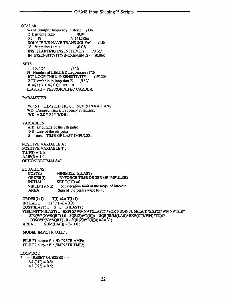
GAMS Input Shaping TM Scripts
SCALAR
WDH Damped frequency in Hertz /1.0/Z Damping ratio /0.0/PI Pi /3.1415926/SOLV IF WE HAVE TRANS SOLV=0
V Vibration Limit /0.05/INS STARTING INSENSITIVITY
IN INSENSITrVrrYoNCREMENTS)
/1.0/
/0.06//0.061;
SETS
I counter /1"3/
N Number of LIMrrED frequencies/1"2/ICT LOOP TttRU INS_SITIVI'I'Y /1"150/
ZCT variable to loop thru Z II'2/EAST(I) LAST COUNTER;ILAST(I) = YES$(ORD(I) EQ CARD(I));
PARAMETER
WP(N') LIMITED FREQUENCIES IN RADIANSWD Damped natural frequency in radians;WE} = 2.0 * PI * WDH ;
VARIABLES
A(I) amplitude of the i th pulseT(I) time of the ith pulseS cost -TIME OF LAST IMPULSE;
POSITIVE VARIABLE A ;POSITIVE VARIABLE T ;
T.UP(I) = I.I;A.UP(I) = 1.0;OPTION DECIMALS=7
EQUATIONSCOST(I)ORDER(I)INITIALVIBLIMrr(N_)AREA
MINIMrT_ T(ILAST)ENFORCE TIME ORDER OF IMPULSES
SET T("I") =0
Set vibration limit at the freqs, of interestSum of the pulses must be 1;
ORDER(I+I) .. T(1) =I.,= T(I+I);INITIAL .. T(" I") =E= 0.0;COST(ILAST) .. S =E= TOLAST) ;VIBLIMIT(N,ILAST) .. EXP(-Z*WP(N)*T(ILAST))*SQRT(SQR(SUM(I,A(I)*EXP(Z*WP(N)*T(1))*
SIN(WP(N)*SQRT(I.0 - SQR(Z))*T(I)))) + SQR(SUM(I,A(I)*EXI:_Z*WP(N)*T(I))*COS(WP(N)*SQRT(1.0 - SQR(Z))*T(1))))) =I._ V ;
AREA .. SUM(I,A(I")) =E= 1.0 ;
MODEL IMP23TR/ALL/;
FILE F1 output file/IMP23TR.AMP/;FILE F2 output file/IMP23TR.TME/;
LOOP(ZCT,* -- RESET GUESSES
A.L('I") = 0.5;A_L('2") = 0.5;
22

GAMS Input Shaping TM Scripts
A.LC3") = 0.0;T.L('2") = 0.52;T.L('3") = 1.0;
--APPROXIMATE TRANSITION FROM 2 TO 3 IMPULSES
IN=0.0635+0.081979*Z+0.25254*SQR(Z);LOOP(ICT,
W'P(" 1") = (WD/SQRT(1.0-SQR(Z)))*(1.0-(0.5*nN));WP("2") = (WD/SQRT(1.0-SQR(Z)))*(1.0+(0.5*IN));
IF (SOLV GE 0.5,SOLVE IMP23TR USING NLP MINIMIZING S ;
* -- Check foranunnecessarythirdimpulseIF ((T.L("3") - T.L("2")) LE .000001,
A.L("2") = A.L("2") + A.L("3");A.L("3") = 0.0;T.L("3") = 0.0;
);IF (A.L("2") LE .000001,
A.L("2") = A.L("3");A.L("3") = 0.0;T.L("2") = T.L("3");T.L("3") = 0.0;
);* -- IF WE FOUND TRAINS SET SOLV TO ZERO AND SKIP REST OF IN
IF (IMP23TR.MODELSTAT EQ 2,IF(A.L("3") GE 0.00001,
SOLV=O.0;);
);PUT FI;PUT @ 1,V:4:2,@6,IN:8:5,@ 15,Z:4:2,@20,A.LC'l"):9:7,@30,
A.L("2"):9:7,@40,A.LC3"):9:7/;IF (IMP23TR.MODELSTAT NE 2,PUT _PUKE'/;
);PUT F2;PUT @ I,V:4:2,@6,IN:8:5,@ 15_:4:2,@20,T.L('2"):9:7_30,
T.L('3"):9:7/;IF (IMP23TR.MODELSTAT NE 2,
PUT 'PUKE'/;* -- HELP A LOST PROGRAM GET BACK ON TRACK
A.L("l")ffi0.5;A.L("2")=0.05;A.L('3")=0.45;T.L("2")=0.28;T.L("3")=0.58;
););IN=IN+0.00001;
);SOLV-I.0;Z=Z+.01;
);
HUMP01TR.gmsSTITLE HUMP01TR
23

GAMS Input Shaping TM Scripts
$OFFUPPER* THIS PROGRAM SOLVES FOR THE INSENSITIVITY AT WHICH THE* SI SHAPER TRANSITIONS FROM 0 HUMPS TO 1 HUMP AS* A FUNCTION OF ZETA.* TURN OFF PRINTING OF MAPS AND SOLVE STATEMENT IN .LST FILE$OFFSYMXREF OFFSYMLIST OFFUELLIST OFFUELXREFOPTION SOLPRINT = OFF;OPTION LIMROW -- 0;OPTION LIMCOL =
SCALARWDH Damped frequency in Hertz /1.0/ZETA Damping ratio /0.0/PI Pi / 3.1415926 /V Vibration Limit /0.02/;
SETSI counter /1"3/
N Number of LIMTI'ED frequencies/1"2/VCT LOOP THRU V/1"11/ZCT variabletoloopthruzeta /1"33/ILAST(I) LAST COUNTER;ILAST(I') = YESS(ORD(D EQ CARD(1));
PARAMETERWD Dampe.d natural frequency in radians;WD = 2.0" PI* WDH ;
VARIABLESIN INSENSrHVH'YWP(N) LIMITED FREQUENCIES IN RADIANSA(1) amplitude of the i th pulseT(I) time of the ith pulseS cost -TIME OF LAST IMPULSE;
POSITIVE VARIABLE A ;POSITIVE VARIABLE T ;POSITIVE VARIABLE IN ;POSITIVE VARIABLE WP ;T.UP(I) = 1.0;A.UP(1) = 1.0;WP.UP(N) = 3*WD;IN.UP = 2;IN.LO = 0.02;
OPTION DECIMALS=7
EQUATIONSCOST(1)ORDER(I)INITIALVIBLII_(N j)AREAZERODERIVEWPI
MmCn_mE TOLAST)ENFORCE TIME ORDER OF IMPULSES
SET T("I")=0Setvibrationlimitatthefxeqs,ofinterest
Sam ofthepulsesmustb¢ IDerivative constraint
SETS WPI BASED ON INSENSITIVITYSETS WP2 BASED ON INSENSITIVITY;
ORDER(I+I) .. TO) =L= T(I+I);INITIAL .. T(" I") =E= 0.0;COST(ILAST) .. S :E: T(ILAST) ;
24

GAMS Input Shaping TM Scripts
VmLEMrrfN_AST).. EXP(-ZETA*WP(N)*TOLAST))* SQRT(SQR(S UM(I,A(I)*EXPCZETA*WP(N)*T(I))*SIN(WP(N)*SQRT(1.0 - SQR(ZETA))*T(I)))) + SQR(SUM(I,Afl)*EXP(ZETA*WP(N)*T(1))*COS(WP(N)*SQRT(1.0 - SQR(ZETA))*T(I))))) =E= V ;
AREA .. SUM(I,A(I))--E=1.0;ZERODERIVCILAST) ..
-ZETA*TCILAS'r)*(SQR(SUMCI,A(1)*EXP(ZETA*WP("2")*T(I))*COS(WP("2")*SQRT(I.0-SQR(Z_A))*T0))))
+SQR(SUM(I,A(I)*EXP(ZETA*WP("2")ST(1))*SIN(WPC2")*SQRT(1.0-SQR(ZErA))*T(1)))))+ SUM(I,A(1)*EXP(ZETA*WP("2")*T(1))*SIN(WP("2")*SQRT(1.0-SQR(ZETA))*T(I)))*(SUM(I,A(I)*Tfl)*SQRT( I-SQR(ZE'rA))*EXP(ZETA*WP("2")*T(I'))*COS (WP("2")*SQRT(1.0o
SQR(ZETA))*T(1)))+ SUM(I,A(1)*T(1)*ZETA*EXP(ZETA*WPC2")*T(T))*SIN(WP("2")*SQRT(I.0-
SQR(ZETA))*T(r))))+ SUM(I,A(1)*EXP(ZETA*WP("2")*T(1))*COS(WP("2")*SQRT(1.0-SQR(ZETA))*T(1)))*(SUM(I,A(1)*T(1)*ZETA*EXP(ZETA*WP("2")*T(1))*COS(WP("2")*SQRT(I.0-
SQR(Z_A))*T(I)))-SUM(I,A(1)*T(1)*SQRT(I-SQRCLETA))*EXP(ZETA*WP("2")*'r('I))*SIN(WP("2")*SQRT(I.0-
SQR(ZETA))*T(1))))=E= 0.0;
EWPI .. WP(" I")=E= (WD*(I.0-(0.5*I/q)))/SQRT(1.0-SQR(ZETA));EWP2 .. W'P("2")=E= (WD*(1.0+(0.5*IN)))/SQRT(1.0-SQR(ZETA));
MODEL HUMPO1TR/ALL/;FILE F1 output file/HUMP01TR.OUT/
LOOP(VCT,A.L('I') = (1+'¢)/4;AJ.,("2") = (I-V)/'2;A-L('39 = (l+V)/4;T.L("2") = 0.45;T.L("3") = 0.9;INJ.. = .17+V;WP.L(" 1") =0.89*WD/S QRT( 1.0-S QR(ZETA));WP./..("2") = 1.1 I*W'D/SQRT(1.0-SQRCZETA));
PUT F1;ZETA= 0.0LOOP(ZCT,
SOLVE HUMP01TR USING NLP MINIMIZING S ;PUT @ 1,V:4:2,@6,IN.L:8:6,@ 15,ZETA:5:3,@22,A.L(" 1"):8:6,@31,
A.L("2"):8:6,@40,A.L("3"):8:6,@49,T.LC2"):8:6,@58,T.L("3"):8:6/;
IF (HUMP01TR.MODELSTAT NE 2,PUT PUKE'/;
);ZETA=ZETA+.OI;
);V=V+.01;
);
FS.gmsST1TLE fs (NEG,SEQ=I)$OFFUPPER* This program IMPLEMENTS FREQUENCY SAMPLING.* The constraints are for an arbitrarily insensitive shaper* TWO PEAKS AND 3 ZERO SLOPE FREQUENCIESSCALAR
25

GAMS Input Shaping TM Scripts
WDH Damped frequency in Hertz/1/ZETA Damping ratio /0.0/PI Pi / 3.1415926 /V Vibration Limit L05/;
SETSI counter /1"5/
N Nmnber of LIMITED frequencies/1"21/mAST(T) LAST COUNTER;mAST_ = YES$(ORD(D EQ CARD(I));
PARAMETER
WL(N) FREQUENCIES TO LIMIT IN PERCENTAGE OF WDH/1 0.802 0.933 0.944 0.955 0.966 0.977 0.988 0.9859 0.9910 0.99511 1.0012 1.0113 1.0214 1.0315 1.0416 1.0517 1.0618 1.0719 1.0820 1.0921 1.20/
WP(N) LIMITED FREQUENCIES IN RADIANSW undamped natural frequencyWD Damped natmal frequency in radiansDELTAW approx distance to touchdown freq. from W;WD = 2.0" PI* WDH ;W = WD I SQRT(I.0 - SQR(ZETA)) ;WP(N) = WL(N)*W;
VARIABLESA(1) amplitude of the i th pulseTO') time of the ith pulseS cost -TIME OF LAST IMPULSECOSSUM(N)SINSUM(N)TZCOSSUM(N)IT_,SINSUM(N)TSQRTZCOS(N)TSQRTZSIN(N)
POSITIVE VARIABLE A ;POSITIVE VARIABLE T ;
* INITIAL GUESSES **T.I..C2") = 0.5/WDH;T.L('3") = 1.0/WDH;T.L("4")= 1.25/WDH;
SUM A.IEXtn2OSSUM AIEXPSIN
SUM AI*TI*ZETA*EXP*COSSUM AI*TI*ZETA*EXP*SIN
SUM AI*TI* SQRTI-Z2*EXP*COSSUM AI*TI* SQRTI-Z2*EXP*SIN;
26

GAMS Input Shaping TM Scripts
T.L("5") = 1.54/WDH;A.L(" 1") -- 0.2625;A.L("2") = 0.475;A.L("3") = 0.2625;
A.L("4") = o.o;A.L("5") = 0.0;COSSUM.L("I") = V-.01;COSSUM.L("2") - V-.01;TSQRTZCOS.L("I") = (.5/WDI-I)*((I.0-V)/2)*COS(W*.5/WDH) +
(1.0/WDH)*((1.0+V)/4)*COS(W* 1.0/WDH);TSQRTZCOS.L("2") --- (.5/WDh0*((1.0-V)/2)*COS(W*.5/WDh0 +
(1.O/WDH)*((1.O+V)/4)*COS(W" 1.0/WI)H);OPTION DECk=6
EQUATIONSCOST(1)ORDER(1)INITIAL
VmL_MrrfN_)AREA
ECOSSUM(N)ESINSUM(N)FrzcossUM(N)ETZSINSUM(N)ETSQRTZCOS(N)ETSQRTZSIN(N)
maximize WZ('3")-wz(" I")ENFORCE TIME ORDER OF IMPULSES
SET T("I") =0set vibration limit at the freqs, of interest
sum of the pulses must be constantSUM AIEXPCOS
SUM AIEXPSINSUM AI*TI*ZETA*EXP*COS
SUM AI*TI*ZETA*EXP*SIN
SUM AI*TI*SQRT1-Z2*EXP*COSSUM AI*TI* S QRT1-Z2*EXP*SIN;
ORDERCI+I) .. T(I') =L= T(I+I);INITIAL .. T(" 1") =E= 0.0;COST(ILAST) .. S =F.,= T(ILAST) ;ECOSSUM(N) .. COSSUM(N) =E= SUM(I,A(I)*EXP(ZETA*WP(N)*T(I))*COS(WP(N)*SQRT(1.0 -
SQR(ZETA))*T(1))) ;
ESINSUM(N) .. SINSUM(N) =E= SUM('I,A(r)*EXP(ZETA*WP(N')'T(I))*SIN(WP(N)*SQRT(1.0 -SQR(ZErA))*T(1))) ;
E'rzcossUM(N) .. TZCOSSUMCN) =E=SUM0.,A(1)*T(I)*ZETA*EXP(ZETA*WP(N)*T(I))*COS(WP(N)*SQRT(1.0 -SQR(ZETA))*T(I))) ;
FI7_,Sn_SUMtN).. TZSINSUM(N) =E=SUM(LA(I)*T(I)*ZETA*EXP(ZETA*WP(N)*T(I))*SIN(WP(N)*SQRT(1.0 - SQR(ZETA))*T(r))) ;
ETSQRTZCOS(N) .. TSQRTT__OS(N) =E= SUM(I,A(1)*T(I)*SQRT(1-SQR(ZETA))*EXP(ZETA*WP(I_D*T(1))*COS(WP(N)*SQRT(1.0 - SQR(ZETA))*T(1))) ;
ETSQRTZSIN(N) .. TSQRTZSIN(N) =E= SUM(I,A(1)*T(I)*SQRT(I-SQR(ZETA))*EXP(ZETA*WP(N)*T(1))*SIN(WP(N)*SQRT(I.0 - SQR(ZETA))*T(I))) ;
VIBLIMIT(N,K.AST) .. EXP(-ZETA*WP(N)*TOLAST))*SQRT(SQR(SINSUM(N)) +SQR(COSSUM(N))) =L= V ;
AREA .. SUM_,A(1)) =E= 1.0 ;
MODEL DAMP/ALL/;
SOLVE DAMP USING NLP MINIMIZING S ;
DISPLAY "Arbitrarily Insensitive", T.L, A.L;
LP.2MOD.gms$'ITrLE LPMOD$OFFUPPER* This PROGRAM FINDS A SEQUENCE USING LEAST SQUARES FOR ONE MODE
* copyright 1994 by Convolve, Inc.
27

GAMS Input Shaping TM Scripts
* TURN OFF PRINTING OF MAPS AND SOLVE STATEMENT IN/..ST FILE*$OFFSYMXREF OFFSYMLIST OFFUELLIST OFFUELXREF*OPTION SOLPRINT = OFF;*OPTION LIMROW =*OPTION LIMCOL = 0;
OPTIONS DECIMAI.S_5SCALAR
DT time spacing /0.05/PI Pi /3.1415926 /
SETSI counter 11"251N Number of SAMPLED f_equencies /1"20/J NUMBER OFFREQU'ENCIES /1"1/ILAST(I) i LAST COUNTERNLAST(N) N LAST COUNTER;ILAST(1) = YES$(ORD(I) EQ CARD(I));NLAST(N) = YES$(ORD(N) EQ CARD(N));
PARAMETERT(I) time of the i )h pulseZ(N) Damping ratio of sample mode N
/1020304050607O8090I0.1II .112.113.114.115.116.117.118.119.120.1/
WSAMP(N) Sampled f_quency data/l 0203040506070809010011012013 014 0
28

GAMS Input Shaping TM Scripts
15 016 017 018 019 0
20 O/WPH(N) THE FREQUENCY SAMPLES FOR LEAST SQUARES Hertz
/1 0.82 0.85
3 0.9
4 0.955 1.06 1.057 1.108 1.159 1.20
10 2.311 2.3512 2.4013 2.4514 2.515 2.5516 2.617 2.6518 2.719 2.75
20 2.8/
WP(N) Sample Frequency in radians;T(I)= DT * (ORD(1) - I);
WP(N) = WPH(N)*2*PI;
VARIABLES
A(1) amplitude of the i th pulseS cost - vl_ralion limit over range of frequenciesV vibrationmagnitude
POSITIVE VARIABLE A ;
EQUATIONSCOST
VmLnvfrrf0AREA
second derivative cost function
LIMIT EI FREQsum of the pulses must be constant;
VlBLIMrr(ILAST).. SUM(N,SQR(WSAMP(N) - SQRT(EXP(-
2*Z(N) *WP(N)*'r(ILAST))*SQR(SUM(I,A(I)*EXP(Z(N)*WP(N)*T(I))*SIN(WP(N)*SQRT(1.0 - SQR(Z(N)))*T(I)))) + SQR(SUM(I,A(I)*EXP(Z(N)*WP(N)*T(I))*COS(WP(N)*SQRT(1.0 - SQR(Z(N)))*T(I))))))) =E= V ;
COST .. S =E= V ;
AREA .. SUM(I,A(1)) =E= 1.0 ;
MODEL LPMOD/ALL/;
SOLVE LPMOD USING NLP MINIMIZING S ;
FILE FI OUTPUT FILE/LPMOD.OUT/;
PUT FI;
loop(l,
IF (A.L(1)NE 0,
PUT @ 1,T(I):8:6,@ 11,A.L(I):8:6/;
29

GAMS Input ShapingTM Scripts
););
Negative Input Shapers
NEGZV.gms$'ITI'LE Neg-ZV$OFFUPPER
* This problem finds a sequence that zeros vibration* minimizing the end time of the sequence, uses Negative Sequences.* The parameter PEAK is the maximum partial sum of the impulses* (See "Design and Implementation of Time-Optimal Negative Input Shapers',* Singhose, Singer, and Seering, 1994 ASME Winter Annual Meeting)
SCALARPI Pi / 3.1415926 /PEAK Peak Partial Sum /1.0/;
SETSI counter /1"3/
J Number of frequencies/1/ILAST(I) last counter ;ILAST(I) = YES$(ORD(I) EQ CARD(T)) ;
ALIAStT,K);
PARAMETER
WDH(J) Damped frequencies in Hertz/1 1.0/
ZETA(J) Damping ratio of mode J/1 0.0/
W(J) undamped natmal frequency JWD(J) Damped natural frequency I in radians ;
WD(J) = 2.0 * PI * WDH(J) ;W(J) = WD(J) / SQRT(1.0 - SQR(ZETA(J))) ;
VARIABLESA(I) amplitude of the i th pulseT('I) time of the i th pulseS cost - Time of last pulse ;
POSITIVE VARIABLE T ;
A.L(':')=PEAK ;A.LC2") = -2.0 * PEAK;A.L('3") = PEAK + 1.0;T.L('I') = 0.0 ;T.L("2") = (0.152406+.2414 I*ZETAC I"))/WDH(" I") - (PEAK- 1.0)*.03;
T.LC'3") = (0.277396+.I0332*ZETA("I"))/WDH('I") - (PEAK-I.0)*.04;OPTION DECIMALS=6
EQUATIONSINIT
COST(1)ORDF._NOVlB_(J)NOVIB2(J)
set initial time valueminimize value of last T
enforce the ordering of the time values
no vibration functionsin partno vFvration function cos part
30

GAMS Input Shaping TM Scripts
AREA
PARTSUM ICK)PARTSUM2(K)
sum of the pulses must be constantpartial sum of the pulses less than onepartial sum of the pulses greater than neg one;
I/fliT .. T("I") =E= 0.0 ;COST(ILAST) .. S =F_,=T(ILAST) ;ORDER(I+I) .. TO') =L= T(I+I);NOVIB l(J) .. SUM(I,A(I')*EXP(ZETA(J)*W(J)*T(I))*SIN(WD(J)*T(I'))) =E---0.0 ;NOVIB2(J) .. SUM(I,A(I)*EXP(ZETA(J)*W(J)*T(I))*COS(WD(J)*T(T))) =E= 0.0 ;AREA .. SUM(I,A(I)) =E= 1.0 ;PARTSUMI(K) .. SUMCI$(ORD(I) LE ORD(K)),A(1)) =L= PEAK ;PARTSUM2(K) .. SUM(I$(ORD(I) LE ORD(IC)),A(I)) =(3= -PEAK ;
MODEL NEGZV/ALL/;
SOLVE NEGZV USING NLP MINIMIZING S ;
DISPLAY A.L, A.M ,T.L, T.M ;
FILE F1 output file/NEGZV.OUT/;PUT F1;PUT @ 1,A.L(" 1"):8:6,@ 10,A2..("2"):8:6,@ 19,A.L("3"):8:6/;PUT @ 1,T.L(" 1"):8:6,@ 10,T.L("2"):8:6,@ 19,T.L("3"):8:6/;
NEGZVD.gmsSTITLE NEGZVD (NEG,SEQ=I)$OFFUPPER
* This problem finds a sequence that zeros vibration and first deriv.* minimizing the end time of the sequence, uses Negative Sequences.* The parameter PEAK is the amount of temporary peak current allowed
SCALARPI Pi / 3.1415926 /PEAK Peak current /4.0/;
SETSI counter / 1"5/
J Number of frequencies/1/ILAST(I) last counter ;ILAST(I) -- YESS(ORD(I") EQ CARD(1)) ;
AL_AS(I,K);
PARAMETERWDH(J) Damped frequencies in Hertz
/1 1.0/
ZETA(J) Damping ratio of mode J/1 0.0/
WfJ) undamped natural frequency JWD(J) Damped natural frequency J in radians ;WD(J) = 2.0 * PI * WDH(J) ;W(J) = WD(J) / SQRT(I.O - SQR(ZETA(J))) ;
VARIABLES
Aft) amplitude of the i th pulseTO') time of the i th pulseS cost - Time of last pulse ;
31

GAMS Input ShapingTM Scripts
POSITIVE VARIABLE T ;
A.L("I") = PEAK ;A.L("2") = -2.0 * PEAK;A.L("3") = 2.0 * PEAK;A.L("4") = -2.0 * PEAK;A.L("5") = PEAK + 1.0;T.L("I") = 0.0 ;T.L("2") = O. 152406+.24141*ZETA(" I"))/WDH(" 1") - (PEAK- 1.0)*.03;T.L("3") = (0.277396+. 10332*ZETA(" 1"))/WDH(" 1") - (PEAK- 1.0)*.04;T.L("4") ---(0.631311+.33061*ZETA(" I"))/WDH(" l") - (PEAK-1.0)*.05;T.L("5") = 0.678948+. 18899*ZETA(" I"))/WDH(" 1") - (PEAK- 1.0)*.05;
OPTION DECIMALS=6DISPLAY A.L, T.L ;
EQUATIONSINITCOST(1)ORDER(I)DERrvl(J)DERIV2(J)NOVmI(J)NOVIB2(J)AREA
PARTSUMI(K)PARTSUM2(K)
set initial time valueminimize value of last Tenforce the ordering of the time valuesfirst derivative function sin partfirst derivative function cos partno vibration function sin partno vibration function cos part
sum of the pulses must be constantpartial sum of the pulses less than onepartial sum of the pulses greater than neg one;
INIT .. T(" 1") =F_,=0.0 ;COST(ILAST) .. S =E= T(ILAST) ;ORDER(I+I) .. TO) =L= T(I+I);DERIVI(J) .. SUM(I,A(1)*Tf0*EXP(ZETA(J)*W(J)*T(1))*SIN(WD(J)*T(I)))
=E= 0.0 ;DERIV2(J) .. SUM(I,A(I")*T(1)*EXP(ZETA(J)*W(J)*T(I))*COS(WD(J)*T('I)))
=E= 0.0 ;NOVIB l(J) .. SUM(I,A(I)*EXP(ZETA(J)*W(J)*T(I))*SIN(WD(J)*T(1))) =E= 0.0 ;NOVIB2(J) ..SUM(I,A(I)*EXP(ZETA(J)*W(J)*T(1))*COS(WD(J)*T(I))) =E= 0.0 ;AREA .. SUIVI(I,A(I))=E= 1.0;PARTSUMI(K) ..SUM(IS(ORD(I) LE ORDCK)),A(I))=L= PEAK ;PAd_.TSUIV[2(IO.. SUMCI$(ORD(I) LE ORD(K:)),A(I))--G=-PEAK ;
MODEL NEGZVD/ALL/;
SOLVE NEGZVD USING NLP MINIMIZING S ;
DISPLAY A.L, A.M ,T.L, T.M ;
NEGEI.gmssTrrLE NEGEI ('NEG,SEQ=I)$OFFUPPER* This program finds a negative Extra-Insensitive shaper for 1 mode.* The time of the last impulse is minimized.* In the presence of damping, the symmetry of the touchdown* frequencies is sacrificed - giving skewed insensitivity.* The vibrationisset equal to VLIM at W and the slopeof* sensitivity curve is forced to zero at that point.* Further, the curve is forced to zero on either side of W.
32

GAMS Input Shaping TM Scripts
SCALAR
WDH Damped frequency in Hertz /1.0/ZETA Damping ratio /0.00/PI Pi / 3.1415927 /VLIM Vibration limit at WDH /0.02/P Input Peak /3.0/;
SETSIL
counter / 1"5 /Number of touchdown frequencies/1"2/
PARAMETER
W undampednannalfrequencyinradiansWD Damped naturalfrequencyinradians
Aft)impulseamplitudesDELTAW approx distance to touchdown freq. from W;A(" I") -- P;A("2") ----2*P;A("3") ---2*P;,A("4") ----2*P;A("5") = P+I;WD= 2.0 * PI * WDH ;W = WD [SQRT(I.0 -SQR(ZETA)) ;
•The followingequationisexactforno damping.The (/*P(I-ZETA)termisahackfordamping.DELTAW = (W/PI)*ARCTAN(2* SQRTCv'LIM)/(I-VLIND)/(P*(I-ZETA));
VARIABLES
TO')time of the i th pulseTW(L) touchdown frequencies (undamped)WP FREQUENCY OF VIBRATION PEAKS cost - distance from TW("2") to TW("I") - maximize thisCOSSUM SUM AIEXPCOSSINSUM SUM AIEXPSINTZCOSSUM SUM AI*TI*ZETA*EXP*COS"[7_,SINSUM SUM AI*TI*ZETA*EXP*SINTSQRTZCOS SUM AI*TI*SQRT1-Z2*EXP*COSTSQRTZSIN SUM AI*TI*SQRT1-Z2*EXP* SIN;
POSITIVE VARIABLE T;POSITIVE VARIABLE TW ;POSITIVE VARIABLE WP ;
* LIMITS ON THE TOUCHDOWN FREQUENCIES **TW.UP(" 1")--W;TW.LO('2") = W;
* INITIAL GUESSES **TW.L('I") = W-DELTAW;TW.LC2") -- W+DELTAW;WP.L = 1.0*W ;
T.LCI') = 0.0 ;T.L('2") = (. 15048+2.6755 *ZETA)*EXP((-.37191-.3471 l*ZETA-
.075744*SQR(ZETA))*LOG(P))/WDH;T.L("3") = (.28746+.12505*ZETA)*EXP((-.1618-.01035*ZETA-
23769" SQR(ZETA))* LOG(P))/WDH;T.L("4") = (.61213+.20742*ZETA)*EXP((-.28491-.15455*ZETA-
.07634*SQR(ZETA))*LOG(P))/WDH;
33

GAMS Input Shaping TM Scripts
T.L("5") = (.67002+.03+.08883*ZETA)*EXP((-.24135-.10405*ZETA-.17039*SQR(ZETA))*LOG(P))/WDH;* THESE HAVE BEEN MANUALLY OVERRIDEN FOR VLIM=0.02, P=3, Z=0
T.L("5")= .518;T.L("4") = .446;T.L("3")= .25;T.L("2")= .I08;
* THESE MAY HAVE TO BE MODIFIED DEPENDING ON P AND ZETA
COSSUM.L = 0.0*VLIM/0.05;SINSUM.L = -.05*VLIM/0.05;
* TSQR'IT.COS.L = 0.004;TSQRTZSIN.L = -0.01;OPTION DECIMALS---6
EQUATIONSINITCOSTORDER03VIBLIMITDERIVWPLWECOSSUMESINSUMETZCOSSUMETZSINSUMETSQRTT__OSETSQR'I"ZSINTOUCHI(L)TOUCH2(L)
set initial time valueminimize t5enforce the ordering of the time valuesset vibration limit at the freq. of interest
deriv constraintINSURES WP Equals W
SUM AI*W*EXI_OSSUM AI*W*EXPSINSUM AI*TI*ZETA*EXP*COS
SUM AI*TI*ZETA*EXP*SINSUM AI*TI*SQRT1-Z2*EXP*COS
SUM AI*TI*SQRT1-Z2*EXP*SINtouchdown of the insensitivity curvetouchdown of the insensitivity curve;
IN1T .. T("I") =E= 0.0 ;COST .. S =E_- T("5");ORDERfI+I) .. T(I) =L= T0+I);WPLW. WP =E= W;ECOSSUM .. COSSUM --E= SUM(I,A(I)*EXP(ZETA*WP*T(I))*COS(WP*SQRT(1.0 -
SQR(ZErA))*T(I))) ;ESINSUM .. SINSUM --E= SUM(I,A(I)*EXP(ZETA*WP*Tfl))*SIN(WP*SQRT(1.0 -
SQR(ZETA))*T(I))) ;ETZCOSSUM. TZCOSSUM=E=
SUM(I,A(r)*T(I)*ZETA*EXP(ZETA*WP*T(I))*COS(WP*SQRT(1.0 - SQR(ZETA))*'r(I))) ;ETZSINSUM .. TZSINSUM =E= SUM('I,A(I)*T(I)*ZETA*EXP(ZETA*WP*T(I))*SIN(WP*SQRT(1.0
- SQR(ZETA))*T(I))) ;ETSQRTZCOS .. TSQRTZCOS =E= SUM(I,A(I)*T(I)*SQRT(1-
SQR(ZETA))*EXP(ZETA*WP*TCD)*COS(W_SQRT( 1.0 - SQR(ZETA))*T(I))) ;ETSQRTZSIN .. TSQRTZSIN =F._.SUM(I,Afl)*T(I)*SQRT(1-
SQR(ZETA))*EXP(ZETA*WP*T(I))*SIN(WP*SQRT(1.0 - SQR(ZETA))*T(I)));VIBUMIT ,. EXP(-ZETA*WP*T("5"))*SQRT(SQR(SINSUM) + SQR(COSSUM)) --F_ VLIM ;
DERIV _ (-ZETA*T("5")*(SQR(COSSUM)+SQR(SINSUM)) + SINSUM*(TSQRTZCOS +TZSINSUM) + COSSUM*('I'ZCOSSUM - TSQRT'Z, SIN))/
(EXP(ZETA*WP*T('5"))*SQRT(SQR(COSSUM)+SQR(SINSUM))) =F.,=0.0;Toucm(L) .. SUM(I,A(I)*KXa'(ZETA*TW(L)*TfD)*
SIN(TW(L)*SQRT(1.0 - SQR(ZETA))*T(I))) --E= 0.0 ;TOUCH2(L) .. sUM fi,A03*F.XPtT_n'A*TW(L)*TfD)*
COS(TW(L)*SQRT(1.0 - SQR(ZETA))*T(I))) =E= 0.0 ;
MODEL NEGEI/ALL/;
34

GAMSInput ShapingTM Scripts
SOLVE DAMP USING NEGEI MINIMIZING S;DISPLAY T.L
Constant-Magnitude Shapers
CAPZV.gmsSTITLE CAFZV$OFFUPPER* This program finds Constant Amplitude Pulses FOR NO VIBRATION.* FOR A TWO MASS- ONE SPRING SYSTEM* The time of the Pulse sequence is minimized.
SCALARWDH Damped frequency in Hertz /1.0/ZETA Damping ratio /0.0/PI Pi /3.1415927/M TOTAL MASS OF SYSTEM /2/;
SETSI counter /1"5/N NUMBER OF LIMITED FREQS /1"1/VCT LOOP THRU VLIM /1"1/ZCT variable to loop thin zeta /1"1/ILAST(I) LAST COUN'IER;ILAST(I) ffiYESS(ORD(I) EQ CARD(I));
PARAMETER
W undamped natural frequency in radiansWD Damped natural f_lueavy in radiansA(I) impulse amplitudes;A('I')--I;A("2"_-2;A('3")=2;A("4")=-2;A("5")_I;WD - SQRT(2.0);W ffiWD / SQRT(1.0 - SQR(ZETA)) ;
VARIABLEST(I) time of the i th pulseD(I) WIDTH OF ITH PULSEWP(N) FREQUENCY OF VIBRATION PEAKS TIME OF TOLAST);
POSITIVE VARIABLE T ;POSITIVE VARIABLE D ;POSITIVE VARIABLE WP ;WP.FX(" I") = WD;OPTION DECIMALSffi6;
T.L('2")_I;TJ.,('3"_=2;T.L('4")=3;T.L('5")=4;
DISPLAY T.L;
EQUATIONS
35

GAMS Input Shaping TM Scripts
IN1T
COST(I)
ORDER(1)FINALPOS
TSE2T3T4E2T3MT2
VmLtMrr(N_
set initial rime value
minimize T(ILAST)enforce the ordering of the time values
MAKES FINAL POSITION =1T5=2T3
T4=2T3-T2
Set vibration limit at the freqs, of interesT;
INIT .. T("I") =E= 0.0 ;COST(ILAST) .. S =E= T(ILAST);ORDER(I+I) .. TO') =L= T(I+I) ;
FINALPOS .. 0.0 =E= 2.0+2*T("2")**2+T("3")**2-4*TC2")*T('3");T5E2T3 .. T("5") =E= 2"T('3");T4E2T3M'I2 .. T('4") =E= 2*T("3")-T("2");VIBLIMIT(N,ILAST)$((ORD(N) EQ 1))
.. EXP(-ZETA*WP(N)*T(ILAST))* SQRT(SQR(S UM(I,A(I)*EXP(ZETA*WP(N)*T(I))*SIN(WP(N)*SQRT(1.0 - SQRCZETA))*T(I)))) + SQR(SUM(I,A(I)*EXP(ZETA*WP(N)*T(I))*COS(WP(N)*SQRT(1.0 - SQR(ZETA))*T(I))))) =E--- 0.0 ;
MODEL CAPZV/ALL/;
FILE F1 output file/CAPZV.OUT/;PUT F1;
SOLVE CAFZV USING NLP MINIMIZING S ;
PUT @ 1,T.L("2"):8:6,@ 10,T.L('3"):8:6,@ 19,T.L('4"):8:6,@28,T.L("5"):8:6/;IF (CAPZV.MODELSTAT NE 2,
PUT PUKE'/;
);
CVCAPZV.gmsSTITLE CVCAPZV$OFFUPPER
* This program f'mde Constant Amplitude Pulses FOR NO VIBRATION* ACCELERATION TO A CONSTANT VELOCITY* FOR A TWO MASS- ONE SPRING SYSTEM
* The time of the Pulse sequence is minimized.* TURN OFF PRINTING OF MAPS AND SOLVE STATEMENT IN .LST FILE$OFFSYMXREF OFFSYMLIST OFFUELLIST OFFUELXREF
OPTION SOLPRINT = OFF;OPTION UMROW = 0;
OPTION LIMCOL = 0;
SCALAR
WD Frequency inRADIANS /1.4142136/Z Damping ratio /0.01
DESVEL /I.01
M1 MASS#1 /I.0/
M2 MASS#2 II.01
PI Pi /3.1415927/;
SETS
I counter /1"4/N NUMBER OF LIMITED FREQSILAST(I) LAST COUNTER;
ILAST(r) = YESS(ORD(I) EQ CARD(I));
/1"1/
36

GAMS Input Shaping TM Scripts
PARAMETER
W undampednaturalfrequencyinindiansWD Damped naturalfrequencyinindiansA(1)impulseamplitudes;A('1")=k0;A("2")=-I.0;A("3")=I.0;
A("4")=-I.0;
VARIABLES
TO) time ofthe ithpulseWP(N) FREQUENCY OF VIBRATION PEAKS TIME OF TOLAST);
POSITIVE VARIABLE T ;POSITIVE VARIABLE WP ;WP.FX("I")= WD;
OPTION DECIMALS=6;T.L("2")=l.437;T.LC3")=2.516;T T("4")=3.597;
DISPLAY T.L;
EQUATIONSINITCOST(1)ORDER(I)DESIREDVELZEROSIN(N)ZEROCOS(I_3
setinitial time valueminimizo T(ILAST)enforcothe ordexing of the time values
MAKES DESIRED VELOCITY = DES'v'ELZERO THE SIN COMPONENT OF VIBRATIONZERO THE COS COMPONENT OF VIBRATION;
INIT _ T(" I") =E= 0.0 ;COST(ILAST) .. S =E= T(ILAST);ORDER(I+I) .. T(1) =L= T('I+I) ;DESIREDVEL .. DESVEL =E= (T("2")-T("3")+T("4"))/(MI+M2);ZF..ROSIN(N) ..
SUM(I,A(I)*EXP(Z*WP(N)*T(1))*SIN(WP(N)*SQRT(1.0 - SQR(Z))*T(I))) =E--- 0.0;ZEROCOS(N) ..
SUM(I,A(I)*EXP(Z*WP(N)*T(I))*COS(WP(N)*SQRT(1.0 - SQR(Z))*T(I"))) =F_.=0.0 ;
MODEL ZV/ALL/;
FILE FI outputfile/CVCAPZV.OUT/;PUT FI;
SOLVE ZV USING NLP MINIIVIIZING S ;
PUT @ I,DESVW_/.:5:3_8,T.L("2"):8:6,@17,T.L("3"):8:6,@26,T.L('4"):8:6/;IF (ZV.MODELSTAT NE 2,
PUT 'PUKE'/;);
CAPEI.gmssTrrLE CAPEI$OFFUPPER
* This program f'mds Constant Amplimdo Pulses FOR NO VIBRATION
37

GAMS Input Shaping TM Scripts
* and EXTRA-INSENSITIVE CONSTRAINTS.* FOR A TWO MASS- ONE SPRING SYSTEM
* The time of the Pulse sequence is minimized.
SCALAR
WDH Frequency in HERTZ /2.0/
Z Damping m,lo /0.0/V VIBRATION LIM1T /0.05/FINPOS FINAL POSITION L07032/PI Pi /3.1415927/;
SETS
I counter /1"7/N NUMBER OF LIMITED FREQSILAST(I) LAST COUNTER;ILAST(I) = YESS(ORD(I) EQ CARD(I));
PARAMETER
/1"3/
W undamped natural fa'equency in radiansWD Damped natural frequency in radians
A(I) impulse amplitudes;A('I")=1.0;A("2")=-2.0;AC3")=2.0;A("4")=-2.0;A('50=2.0;A('6"3=-2.0;A("7")=I.0;WD=WDH*2*PI;
VARIABLES
T(r) time of the i th pulseWP(N) FREQUENCY OF VIBRATION PEAKS TIME OF T(ILAST);
POSITIVE VARIABLE T ;
POSITIVE VARIABLE WP ;WP-LC I') = .95*WD;wP.Fx(-2-) =WD;WPLC'3") = 1.05*WD;WP.LO('I')= 0.7*WD;WP.UP(N)= 1.3*WD;OPTION DECIMALS=6;
T.LC2")=0.179;T.L("3")=0.236;TrT.L('5")=0.646;T.LC6")=0.703;
T.LC7")=0.882;T.UP(I) = 1.2;
EQUATIONSINIT
COST(1)
ORDER(1)ORDERWP(N)FINALPOSZEROSUM
set initial time value
minimize T(ILAST)
enforce the ordering of the time valuesORDER WPS
MAKES FINAL POSITION = DESIRED
SUM OF PULSES EQUAL ZERO
38

GAMS Input Shaping TM Scripts
VlBLIMIT(N,I)ZVIBLIM1T(N,I)ZERODERIV(N,I)
Set vibration limit at the freqs, of interesTZERO vibration at the freqs, of interesT
ZERO THE DERIVATIVE AT WD;
INIT .. T(" 1") =E= 0.0 ;COST(ILAST) .. S =E= T(ILAST);ORDERWP(N+t) .. WP(I'0=L= WP(N+I);ORDER(I+I) .. TO') =L= T(I+I) ;FINALPOS .. FINt_S =E= 0.5"(-(TC'2")*'2) + T("3")*'2 - cr("4")*'2)
+T("5")**2 -(T("6")*'2) -0.5"T("7")*'2+2*T('2")*T("7") -2*T('3")*T("7")+2*T("4")*T("7")-2*T('5")*T("7 ") + 2*T('6")*T("7"));
ZEROSUM .. 0.0 =E= T("2")-T('3")+T("4")-T("5")+TC6")-0.5*T("7");VmLtMrr ,a.. ST)$(OI D(N) r:Q2)
.. EXP(-Z*W'P(N)*TOLAST))* SQRT(SQR(SUM(I,Afl)*EXP(Z*WP(N)*T(I))*SIN(WP(N)*SQRT(1.0 - SQR(Z))*T(I)))) + SQR(SUM(I,A(r)*EXP(Z*WP(N)*T(I))*COS(WP(N)*SQRT(1.0 - SQR(Z))*Tff))))) =F,= V ;
ZVIBLIMIT(N,K,AST)$((ORD(N) EQ l) OR (ORD(N) EQ 3)).. EXP(-Z*WPfN) *TCILAST))* SQRT(S QR(SUMCI,Afl)*EXP(Z*WP(N)*T(T))*SIN(WP(N)*SQRT(1.0 - SQR(Z))*T(I)))) + SQR(SUM(I,Afl)*EXP(Z*WP(N)*T(I))*COSOVP(N)*SQRT(1.0 - SQR(Z))*T(I))))) =L= 0.0001 ;
ZERODERIV(N,ILAST)$(ORD(N) EQ 2).. -EXP(-T(ILAST)*WP(N)*Z)* {Z*T(ILAST)*SQRT(SQR(SUM(I,A(I)*EXP(Z*WP(N)*T(I))*COS(WP(N)*SQRT(1.0 -
SQR(Z))*T(I))))+ SQR(SUM(I,A(I)*EXP(Z*WP(N)*T(I))*SIN(WP(N)*SQRT(1.0 - SQRC'Z))*T(I)))))+ { SUM(I,A(I)*EXP(Z*WP(N)*T(I))*COS(WP(N)*SQRT(1.0 - SQR(Z))*T(I)))*SUM(I,A(I)*T(I)*EXP(T(I)*WP(N)*Z)* (SQRT(1 -SQR(Z))*SIN(T(T)*WP(N)*SQRT(1 -SQR(Z)))-Z*COS(T(I)*WP(N)* SQRT(1-SQR(Z)))))- SUM(I,A(I)*EXP(Z*WP(N)*T(I))*SIN(WP(N)*SQRT(1.0 - SQR(Z))*T(I)))*SUM(I,A(I) *T(I)*EXPO'('I)*WP(N)*Z)* (SQRT( 1-S QR(Z))* COS (T('f)*WP(N)* SQRT( 1-SQR (Z)))+Z* SIN(T(I)*WP(N)*SQRT(1-SQR(Z))))) }/(SQRT(SQR(SUM(I,A(I)*EXP(Z*WP(N)*T(1))*COS(WP(N)*SQRT(1.0 -SQR(Z))*T('I))))+ SQR(SUM(I,A(I)*EXP(Z*WP(N)*T(I))*SIN(WP(N)*SQRT(1.0 -SQR('Z))*T(r)))))) }
=E= 0.0;
MODEL CAPEI/ALL/;
FILE F1 output file/CAPEI.OUT/;PUT F1;
WD=-WDH*2*PI;WP.FX('2") = WD;
SOLVE CAPEI USING NLP MINIMIZING S ;
PUT @ 1,WDH:6:4,@ 10,T.L('2"):8:6,@ 19,T.L("3"):8:6,@28,T.L('4"):8:6,@ 37,T.L("5"):8:6,@46,T.L("6"):8:6,@ 55,T.L("7"):8:6/;
PUT @ 1,WDH: 6:4 ,@ 10,T.L('2"):8:6,@ 19,(T.L('3")-T.L("2")): 8:6,@ 28,(T.L('4")-T.L("3")):8:6,@37,(T.LC'5")-T.L("4")):8:6,@46,(T.L("6")-T.L("5")):8:6,@ 55,(T.L("7")-T.L("6")):8:6/;
IF (CAPEI.MODELSTAT NE 2,PUT "PUKE'/;
);
39
MATLAB Input Shaping TM Toolbox
Copyright Convolve, Inc., 1995
This document describes Convolve's Input Shaping Toolbox. The functionsdescribed are used for generating vibration-reducing commands to dynamic systems. Thisdocument contains three sections. First, Every function in the toolbox is listed. Second, abrief description is given for most of the commands. Finally, the header fries from eachfunction are listed. The last two sections are available on-line in MATLAB by typing"help Contents"and
"help READ_ME".

Universal_IS_Toolbox
Name Size Kind Label Last Modified
[] ACC2TRAP.M
D ACTTF.M
CIRCLE.M
[] CIRCLEP.M
[] CON2DIG.M
D CON_WrS.M[] CONVOLVE.M[] CRMETRIC.M
[] DIG2CON.M
[] DIGEI5.m
[] DIOS_-Q.M
[] DigZVD5.m
[] DVD.M[] _I.MD EL_HUMP.M[] EI2M_DMP.M
[] EI2M_UND.M
D n3mSMr.M[] El.. UNDMP.M
[] GETACCEL.M
[] GPLANE.M
[] MDSmERA.M[] MDSrZERJ.M
[] NEG2MZVD.M
[] NEGEI.M
[] NEGZV.M
[] NEGZVD.M
[] NMASSSYS.M
[] NO_W.M[] PRESR.M
[] PRETF.M[] a>a'2MZV.MD RAP2MZVD.M
[] Rapp9Seq.m
[] READ_ME.m[] RESID.M
2K MATLAB
2K MATLAB
2K MATLAB
2K MATI.AB
2K MATLAB
6K MATI.AB
2K MATLM3
4K MATLAB
2K MATLAB
4K MATLA.B
2K MATLAB
2K MATLAB
2K MATLAB
2K MATI_AB
2K MATLAB
2K MATLAB
2K MATLAB
2K MATLAB
2K MATLAB
2K MATLAB
2K MATLAB
2K MATLAB
4K MATLAB
2K MATLAB
4K MATLAB
2K MATLAB
2K MATLAB
4K MATLAB
2K MATLAB
4K MATLAB
2K MATLAB
2K MATLAB
2K MATLAB
4K MATLAB
22K MATLAB
4K MATLAB
document
document
document
document
document
document
document
document
document
document
document
document
document
document
document
document
document
document
document
document
document
document
document
document
document
document
document
document
document
document
document
document
document
document
document
document
Sun, Sep 12, 1993, 5:19 PM
Sun, Jan 22, 1995, 11:24 PM
Sun, Jan 22, 1995, 11:25 PM
Sun, Jan 22, 1995, 11:26 PM
Sun, Sep 12, 1993, 5:19 PM
Mon, Jan 23, 1995, 12:28 AM
Thu, Aug 19, 1993, 2:29 PM
Fri, Sep 17, 1993, 11:29 PM
Sun, Sep 12, 1993, 5:20 PM
Sun, Jan 22, 1995, 11:32 PM
Sun, Sep 12, 1993, 5:22 PM
Mon, Jan 23, 1995, 12:00 AM
Sun Dec 5, 1993, 3:54 PM
Sun Jan 22, 1995, 8:25 PM
Sun ]'an 22, 1995, 8:27 PM
Sun Jan 22, 1995, 9:58 PM
Sun Jan 22, 1995, 8:23 PM
Sun Jan 22, 1995, 8:26 PM
Sun Jan 22, 1995, 8:25 PM
Sun Sep 12, 1993, 5:23 PM
Mon, ]'an 23, 1995, 12:03 AM
Sat, Sep 18, 1993, 5:41 PM
Mon, Sep 13, 1993, 9:47 PM
Sun Jan 22, 1995, 8:18 PM
Sun ]'an 22, 1995, 8:00 PM
Sun ].an 22, 1995, 8:05 PM
Sun ]'an 22, 1995, 8:05 PM
Sun Jan 22, 1995, 8:08 PM
Tue Jul 13, 1993, 1:43 PM
Mon, Jan 23, 1995, 12:06 AM
Fri, Jan 4, 1980, 8:10 AM
Sun, Jan 22, 1995, 8:10 PM
Sun, Jan 22, 1995, 8:03 PM
Thu, Oct 14, 1993, 10:06 AM
Mon, Jan 23, 1995, 12:25 AM
Mon, Jan 23, 1995, 12:08 AM

Name
Universal_IS_Toolbox2
Size Kind Label Last Modified
D SENSPLOT.M
[] SENSPLT2.M
[] SEQCONV.M
rl SEQSORT.M
[] SHAPGEN.M
rl SHAPRES.M
[] SPEEDCRM.M
[] TRAPPROF.M
[] TRAP_RUL.M
[] TWOMASS.M
D VD.M
[] w DICSEq.M
[] ZV.M[] ZVD-2M.M[] ZVD.M[] ZVD2MD.M
[] ZVDD.M
[] ZVDDD.M
2K MATLAB document --
2K MATLAB document --
2K MATLAB document --
2K MATLAB document --
6K MATLAB document --
2K MATLAB document --
2K MATLAB document --
2K MATLAB document --
2K MATLAB document --
2K MATLAB document --
2K MATLAB document --
21( MATLAB document --
2K MATLAB document --
2K MATI_.4.B document --
2K MATLAB document --
2K MATLAB document --
2K MATLAB document --
2K MATI_..4_ document --
Sun
Sun
Sun
Sun
Wed.
Sun
Mon
Sun
Mon
Thu
Sun
Thu
Sun
Sun
Sun
Sun
Sun
Sun
Jan 22, 1995, 8:13 PM
lan 22, 1995, 8:15 PM
Sep 12, 1993, 5:26 PM
Sep 12, 1993, 5:26 PM
Nov 3, 1993, 1:15 PM
Sep 12, 1993, 5:27 PM
Sep 20, 1993, 3:21 PM
Sep 12, 1993, 5:32 PM
Jan 23, 1995, 12:22 AM
Aug 26, 1993, 6:14 PM
Dec 5, 1993, 3:56 PM
Sep 9, 1993, 10:20 PM
Jan 22, 1995, 8:06 PM
Jan 22, 1995, 8:21 PM
Jan 22, 1995, 8:19 PM
Jan 22, 1995, 8:11 PM
Jan 22, 1995, 8:20 PM
Jan 22, 1995, 8:2I PM

Contents.M
% Input Shaping Toolbox, Copyright Convolve, Inc 1993 9/9/93%%
% Input Shaping Toolbox%
% One-mode Shapers%
% EI:A three-impulse sequence that limits the vibration to V at the% modeling frequency, (instead of forcing it to zero), to acheive
% larger amounts of insensitivity than the ZVD shaper. Shaper length% equals 1 period. The shaper works well for 0<V<.2 arts 0<zeta<.25.°k EI2HUMP: A 4-impulse shaper that has two humps in its sensitivityok curve. It has the same length as a ZVDD, but has a larger% insensitivit-v to modelling errors.ok EI3HUMP: A 5-_mpulse shaper that has three humps in its sensitivity% curve. It has the same length as a ZVDDD, but has a larger% insensitivity, to modelling errors.% EI_UNDMP: An exact EI shaper for 1 UNDAMPED mode. Shaper length
% equals 1 period of vibration.% DIGEI5: An exact digital EI shaper, using matrix inversion technique.
% DIGZVD5: An diNtal ZVD shaper calculated by linearizing the% times to the nearest two time discrete time steps and% then inve_ing the matrix of the original equations.% NEGEI: A negative EI shaper for 1 mode. This shaper is shorter% than the positive EI. The amount of overcurrenting is% controlled with the parameter P. For P= 1, the negative% shaper is approximately 30% shorter than the positive EI.ok NEGZV: A negative ZV shaper for I mode.ok NEGZVD: A negative ZVD shaper.
ok ZV : A two-impulse sequence that gives no vibration at% the modeling frequency, but has poor insensitivity.
% Shaper length equals 1/2 period of vibration.% ZVD : A three-impulse sequence that has both zero vibration% and zero slope of the sensitivity curve at the modeling% frequency. Shaper length equals 1 period of vibration.°k ZVDD :A four-impulse sequence that has zero vibration and zero 1st% and 2nd derivatives of the sensitivity curve at the modelingok frequency. Shaper length equals 1.5 periods of vibration.% ZVDDD:A five-impulse sequence that has zero vibration and zero 1st% 2nd, & 3rd derivatives of the sensitivity curve at the modeling
% frequency. Shaper length equals 2 periods of vibration.%
ok Two-mode Shapers% EI2M_DMP: An EI shaper for 2 modes. The solution comes from a surfaceok fit to data calculated with GAMS. The shaper works well overok the ranges of 0<V<.2 ans 0<z<.25. The shapers for each mode
% are convolved together to give the final shaper.% EI2M_UND: An exact EI shaper 2 UNDAMPED modes. The shapers for eachok mode are convolved together to give the final shaper.% NEG2MZVD: A negative 2 mode ZVD shaper based on Rappole eqns.% This shaper is shorter than a 2 mode shaper formed

% by convolving two single-mode shapers together.
% RAP2MZV: A 2 mode ZV shaper based on Rappole equations for 2% undamped modes. This shaper is shorter than two% single-mode ZV shaper convolved together. Do not use% this for frequency ratios over 3.76679 - it will
% result in gains larger than one (overcurrenting).
% RAP2MZVD: A 2 mode ZVD shaper based on Rappole equations for 2% undamped modes. This shaper is shorter than two% single-mode ZVD shaper convolved together. Do not use% this for frequency ratios over 3.76679 - it will
% result in gains larger than one (overcurrenting).% RAPP9SEQ: An exact digital sequence found with Rappole 2-modes,% 5-impulse constraints. Uses matrix inversion.
% ZVD-2M : A two-mode shaper that uses two ZVD shapers convolved% together. Shaper length equals the sum of the two periods.% For a shorter 2-mode shaper see ZVD2MD.% ZVD2MD: A two-mode shaper that uses ZVD constraints. The solution
is based on the result of a curve fit to data from GAMS.
The shaper length is shorter than the sum of the two periods.The shaper works well for 1.2<r<2.8 and 0<z<.15.
%%%%%%%
Trapezoidal Profiling Utilities
% Acc2Trap : Calculate a shaped trapezoidal trajectory (both% velocity, and position) using an acceleration table
% TrapProf : Generate position and velocity commands for a trapezoidal% velocity, profile.%%
% Additional Input shaping utilities%
% Convolve : Covolves Input and Shaper and returns the% result ShapedInput.% Dig2con : Put a digital sequence in continuous
% DigSeq : Map a sequence onto digital timing loop% SeqConv : Convolve two continuous sequences together.% SeqSort : Sort a continuous sequence into correct% order and combine impulses at the same time.
% ShapRes • Calculate the residual for a given freq and zeta% Con2Dig • Puts a continuous sequence in digital sequence form.%
% SensPlot : Plot the residual over range of frequencies%
% Dig3Imp : Finds a digital sequence for a ThreeImpSeq by linearizing% the times to the nearest two time discrete time steps and% then inverting the matrix of the original equations% W_DigSeq : Uses Watanabe's formula to split each continuous% impulse into two digital impulses

%%READ_ME.m%This file containstheheadersfrom all of the% functionsin theInput ShapingToolbox.% For abrief descriptionof all thefunctionsin this% toolbox, seeCONTENTS.M%% [T,V,P] = acc2trap(Accel,dt)%% Calculateashapedtrapezoidaltrajectory(both% velocityandposition)usinganaccelerationtable% Thetableis generatedby GETACCEL.%% Parameters:% Accel- AccelerationTablefrom GETACCEL% dt - timestepfor system(sec/step)%% Returns:% T - A time vector [0 dt 2dr ....];% V - A velocity vector.% P - A positionvector.% All outputshavethesamelength.%% SeealsoGETACCEL.%%ACTI'F.M% Actuatorlaplacetransformanalysisfor systemswith andwithout% pref'flters.% For asystemwithout aprefilter thetransferfunctionfrom the% referenceinput to theactuatoris givenby CLS(s)/OLP(s)where% CLS(s) is theclosedloopsysstemresponsetransferfunction.% OLP(s)is the openloop systemresponsetransferfunction.% For asystemwith a preftlter the transfer function from the% reference input to the actuator is given by PRE(s)*CLS(s)/OLP(s)% where PRE(s) is the prefilter transfer function.%% CIRCLE.M
% plots the root locations of the polynomial around in the unit circle%% CIRCLEP.M
% plots the root locations of the polynomial around in the unit circle%
% con2dig CONTINUOUS2DIGITAL Put a continuous sequence in digital% sequence form.%
% dseq = con2dig(cseq,dt)%
% A continuous sequence is an n*2 matrix with times (see) in% the first column and amplitudes in the second column.% A digital sequence as a vector of amplitudes, where each% value corresponds to a time step. The vector has length% n = Time Of Last_Impulse/tit.%

%Parameters:% cseq,thecontinuoussequence.Assumesthatthe% continuoussequenceis spacedat intervalsof tit.% dt, thetime stepfor thedigital sequence.%% Returns:% dseq,thedigital sequence.%% Seealso DigitizeSeq, Digital2Continuous%
% Convolve(Input,Shaper,deltaT) -- Bill Singhose% Covolves Input and Shaper and returns the result ShapedInput.% A time vector, T, which has the same number of rows as
% ShapedInput is also returned. T starts at zero and is incremented% deltaT each step.% Input can be an nxm matrix,where m is the number of inputs.% Shaper must be a row or column vector.%
% Function CRMETRIC(a,b,c,d,T)
% [FIRy,FIRact,PRE,TFIR,resid,s]=crmetric(a,b,c,d,T)% "Controller Redesign Metric"
% Given a continuous system description [a,b,c,d], where% the fast and second outputs are position and actuator% effort, computes the FIR components of the response for% the two outputs and the overall prefflter time period TFIR%
% DIG2CON Put a digital sequence in continuous sequence form.%
% cseq = dig2con(dseq,dt)%
% A continuous sequence is an n*2 matrix with times (sec) in% the fast column and amplitudes in the second column.% A digital sequence as a vector of amplitudes, where each% value corresponds to a time step. The vector has length% n = Time Of Last_Impulse/dt. •%% Parameters:
% dseq, the digital sequence.% dt, the time step for the digital sequence.%% Returns:
% cseq, the continuous sequence.%
% seq = DIGEI5(dt,freq,zeta, vlim)
% Find an exact digital Extra-Insensitive shaper.% Uses matrix inversion technique.%
% digseq - Whit Rappole% DIGITIZESEQ Map a sequence onto digital timing loop% dseq ---digseq(seq,step)%
% Uses a linear extrapolation to split each continuous% impulse into two digital impulses%

% seq= DigSeq(dt,freq,zeta)%% Findsadigital ZVD shaperby linearizing% thetimesto thenearesttwo timediscretetime stepsand% theninverting thematrix of theoriginalequations%% seq= DigZVD5(dt,freq,zeta)% Findsa digitalZVD shaperby linearizing% thetimesto thenearesttwo timediscretetime stepsand% theninverting thematrix of theoriginalequations%%functiondvd(amp,freq,zeta,dt)% or vd(digital_shaper,freq,zeta,dt)% createsavectordiagrambasedonthe% providedf (naturalfrequencyin hertz)% andthetimestep(dt) andamplitudesof thepulses%% Mappingis -> theta= w'time% Soeachvectoramp[i],time[i] hasacorresponding% positionin thevectordiagram.%% Currentlyonly handlespositivevectorsamp= [t3to 1]%%EI(fd,z,V,deltaT)-- Bill Singhose% GeneratesanEI shaperfor 1mode.%Thesolutioncomesfrom a surfacefit to datacalculatedwith GAMS.% Theshaperworkswell overtherangesof 0<V<.2 arts0<z<.25% fd - dampedfrequency(Hz) of vibrationbeingcontrolled.% z - dampingratioof vibrationbeingcontrolled.%V - vibration limit, for 5%vibration;Vlim=0.05.%deltaT- time spacingat which input to systemis updated.%%%EI2HUMP
% Generates a two-hump EI shaper% f- frequency (Hz) of vibration being controlled.% V - vibration limit
% deltaT - time spacing at which input to system is updated.'%
% This function generates the exact sequence and then uses% DigSeq to convert the exact sequence to digital format.%
% % EI2M_DMP(fd 1,fd2,z 1,z2,_" 1,V2,deltaT) -- Bill Singhose% Generates an EI shaper for 2 modes.% The solution comes from a surface fit to data calculated with GAMS.
% The shaper works well over the ranges of 0<V<.2 ans 0<z<.25% The shapers for each mode are convolved together to give the% final shaper.% fdl,fd2 - frequency (Hz) of damped vibration being controlled.% zetal,zeta2 - damping ratios of vibration being controlled.% Vliml,Vlim2 - vibration limits, for 5% vibration, Vlim---0.05.
% deltaT - time spacing at which input to system is updated.%
%% EI2M_UND(fl,f2,Vliml,Vfim2,deltaT) -- Bill Singhose% Generates an EI shaper 2 UNDAMPED modes.

% (Thevibrationat themodelingfrequencyis limited to Vlim% andtheinsensitivityismaximized)% Theshapersfor eachmodeareconvolvedtogetherto givethe% final shaper.% fl,f2 - frequency(Hz) of vibrationbeingcontrolled.% Vliml,Vlim2 - vibration limits, for 5%vibration, Vlim--0.05.% deltaT- time spacingat which input to systemis updated.%%%EI3HUMP% Generatesathree-humpEI shaper% f - frequency(Hz) of vibrationbeingcontrolled.%V - vibrationlimit% deltaT- time spacingatwhich input to systemis updated.%% This functiongeneratestheexactsequenceandthenuses% DigSeqto converttheexactsequenceto digital format.%%%EI_UNDMP(f,Vlim,deltaT) -- Bill Singhose% GeneratesanEI shaperfor 1UNDAMPED mode.% (Thevibrationatthemodelingfrequencyis limited to Vlim% andtheinsensitivityis maximized)% f- frequency(Hz)of vibrationbeingcontrolled.% Vlim - vibration limit, for 5%vibration,Vlim---0.05.% deltaT- time spacingat which input to systemis updated.%%%getaccel(seq,vmax,amax,des,dt)%% Getanaccelerationmatrixfor calculatingshaped% trapezoidaltrajectoriesusingchangingaccelerations.%%% GPLANE.M% G planeanalysisof theresponseof asecondordersystemto damped% sinusoidinputs.%%%MDSIZER - Pointto Pointmoveprofile basedonagivenAccelerationPulse
[x,v,a,nd]=mdsizer(Dist,AccSeq,T)For anAccSeq[1 1 1... 1 1 1],mdsizerageneratesa trapezoidalvelocity profile.
%%%%%%%%%%%%%%%%%
INPUTS:
Dist - move distance
AccSeq - acceleration sequenceT - sample period
OUTPUTS:
x - positionv - velocitya - acceleration
nd - sample delay before start of second pulse.
% NOTE: the derivation involved using the f'mal value theorem and in% the model used, zero order holds were assumed.

%% An arbitraryaccelerationpulseiscombinedwith anegativeanddelayed% (byndsamples)versionof thepulseto generatetheoverall% accelerationprofile. If thedesiredmovedistance(dist)cannotbe% achievedwith an integerdelay(nd), thenthedelayis roundedup to% thenextintegervalueandtheaccelerationpulsescaleddownto meet% thedesiredmovedistance(dist). Notethat for veryshortmoves,(nd)%approacheszero,andthelengthof theoverallaccelerationprofile%approachesthatof thearbitraryaccelerationpulse.This functionis%designedto beusedwith accelerationpulsesthathavebuilt in%vibrationcancellationandthisiswhy thepulseshapeis notmodified%in thecaseof shortmoves.%Note,the lengthof thesequences[x], [v], and[a] aredifferentdue%to apole/zerocancellationthatoccursduringintegration.%%%MDSIZERJ- Point to Pointmoveprofile basedonagivenJerkSequence
[x,v,a,nd]=mdsizer(Dist,JerkSeq,T)For a JerkSeq[1 0 0 ...0 0 -1], mdsizergeneratesatrapezoidvelocity profile.
%%%%%%%%%%%%%%%%%
INPUTS:
Dist - movedistanceJerkSeq- jerk sequenceT - sampleperiod
OUTPUTS:
x - positionv - velocitya- acceleration
nd- numberof sampledelaysbetweenstartof pulses
% NOTE:thederivationinvolvedusingthefinal valuetheoremandin% themodelused,zeroorderholdswereassumed.%% An arbitraryaccelerationpulseiscombinedwith anegativeanddelayed% (by ndsamples)versionof thepulseto generatetheoverall% accelerationprof'de. If thedesiredmovedistance(dist)cannotbe% achievedwith anintegerdelay(nd),thenthedelayis roundedup to% thenextintegervalueandtheaccelerationpulsescaleddownto meet% thedesiredmovedistance(dist). Notethatfor very shortmoves,(nd)% approacheszero,andthelengthof theoverallaccelerationprofile% approachesthatof thearbitraryaccelerationpulse. This functionis% designedto beusedwith accelerationpulsesthathavebuilt in% vibrationcanceUationandthis iswhy thepulseshapeis notmodified% in thecaseof shortmoves.% Note,the lengthof thesequencesIx], [v], and[a]aredifferentdue% to apole/zerocancellationthatoccursduringintegration.%%%NEG2MZVD(fl,dt)%NEG2MZVD Generatesanegative2modeZVD shaper%basedonRappoleequations%

% fl - Frequencyto shapefor (Hz.)%deltaT- Time spacing(sec/step)%%%NEGEI(f,zeta,V,PdeltaT)--Bill Singhose%GeneratesanegativeExtra-Insensitiveshaperfor 1mode.%%Returnsthedigital sequenceby default,and%theexactsequenceasthesecondvariable:%eg: togeneratetheexactshaper,use:% [dig_shaper,exact_shaper]=singer13(f,z,0.01)% note: the0.01is ignoredfor theexactshaperand% dig_shapercanbeignored%% to Returnthedigital sequence,use:% dig_shaper=singerl3(f,z,0.001)%% f- frequency(Hz)of vibrationbeingcontrolled.% zeta- dampingratioof vibrationbeingcontrolled.%V - VibrationLimit% P- Input Peak%deltaT- time spacingatwhich inputto systemisupdated.%%This functiongeneratestheexactsequenceandthenuses%DigitizeSeqto converttheexactsequenceto digital format.%%%negzv(f,zeta,deltaT)--Bill Singhose%GeneratesanegativeZV shaperfor 1mode.%%Returnsthedigital sequenceby default,and%theexactsequenceasthesecondvariable:%% to Returnthedigital sequence,use:% dig_shaper=-negzv(f,z,0.001)%% f - frequency(Hz) of vibrationbeingcontrolled.% zeta- dampingratioof vibrationbeingcontrolled.% P - InputPeak% deltaT- timespacingatwhich inputto systemis updated.%%This functiongeneratestheexactsequenceandthenuses% DigitizeSeqto converttheexactsequenceto digital format.%%%NEGZVD(f,zeta,deltaT)--Bill Singhose% GeneratesanegativeZVD shaperfor 1mode.%% Returnsthedigital sequenceby default,and% theexactsequenceasthesecondvariable:%eg: to generatetheexactshaper,use:%%%%%%
[dig_shaper,exact_shaper]=singer13(f,z,0.01)note: the0.01is ignoredfor theexactshaperand
dig_shapercanbe ignored
to Returnthedigital sequence,use:dig_shaper=singer13(f,z,0.001)

%%%%%%%%%%%%%%%%%%%%
%% f - frequency(Hz) of vibrationbeingcontrolled.%zeta- dampingratioof vibrationbeingcontrolled.% P - Input Peak% deltaT- timespacingat whichinputto systemis updated.%%%NMASSSYS [a,b,c,d]=nmasssys(m,k,gains)% Createsastatespacemodelof ann masssystemandreturns
the [a,b,c,d]matricesof thesystem.[m] is avectorof masses(theinput forceactsonmassm(1)).[gains]is avectorof feedbackgains,(+) for negfeedback;
to build amodelwithoutfeedbackuseanull matrix []for gains.
[k] is a vectorof springsbetweenthemasses;k(1) isbetweenmassesm(1) andm(2); apicturefollows:
F-->m(l)--k(1)--m(2)--k(2)--m(3)--...
Systemoutputy = [xl act]'
Where: act- forceoutputof idealactuatoractingonmass1;thetransferfunctionof theactuatoris 1/1.xl - positionof themassbeingpushedby act(mill).
If "gains"exists,thennegativefeedbackof thestatesxldot,xl,x2dot,x2 .... is includedin thestatespacemodel.
%% [PN,wn]=NORMP(P1)%Normalizesacharacteristicpolynomialsuch%thattherearedecendingpowersof S from theleft anddecending%powersof W from theright (rightmostandleftmostcoefficientsare%alwaysunity. ReturnsthenormalizedpolynomialandtheWN usedin%thenormalization.Polynomialsshouldbeenteredsuchthatthe% coefficientof thehighestpowerof S is unity.%%% PRESR.M% Stepresponsefor secondordersystems(res)andstepresponsefor% secondordersystemswith athreeimpulseprefilter (resp)%%%PRETF(Z,W,S)evaluatesthetransferfuctionof athreeimpulseprefilter% designedfor asystemwith thegivenz andw, at thegivenvalueof% thecomplexvariables.%%%RAP2MZV(fl,f2,deltaT) -- Bill Singhose% Generatesa2 modeZV shaperbasedon% Rappoleequationsfor 2 undampedmodes.% Donot usethis for frequencyratiosover3.76679- it will% resultin gainslargerthanone.% fl, f2 - frequencies(Hz)of vibrationbeingcontrolled% deltaT- timespacingatwhich inputto systemis updated%%%RAP2MZVD(fl,f2,deltaT) -- Bill Singhose%Generatesa2 ModeZVD shaperonbasedRappoleequations

% for 2 undampedmodes.% Do notusethis for frequencyratiosover3.76679- it will% resultin gainslargerthanone.% fl, f2 - frequencies(Hz)of vibrationbeingcontrolled%%%seq= Rapp9Seq(dt,fl,zl,f2,z2)%Findanexactdigital sequencefoundwith Rappole2-modes,% 5-impulseconstraints.%Usesmatrix inversiontechnique.%%%RESID.M%residueanalysisof dynamicsystems%%%sensplotPlot theresidualoverrangeof frequencies%% list = sensplot(seq,fmin,fmax,zeta,points)%% seqis theshapingsequence% fmin is the low endof thefrequencyrange% fmaxis thehighendof thefrequencyrange%zetais thedampingratioof thesystem%pointsis thenumberof pointsto calculate%%%SEQUENCECONVOLVEConvolvetwo continuoussequencestogether.%% seq= seqconv(seql,seq2)%%Convolvestwo sequencestogether.%A Sequenceis ann*2 matrixwith impulsetimes(sec)in%thefirst columnandamplitudesin thesecondcolumn.%%Parameters:% seq1,seq2thetwo sequencesto convolvetogether.%%Returns:% seq,thesequenceresultingfrom theconvolution.%%%SEQUENCESORTSortacontinuoussequenceinto correct% orderandcombineimpulsesatthesametime.%% sortedseq= seqsort(unsortedseq)%%A sequenceis ann*2 matrixwith times(sec)in thefirst% columnandamplitudesin thesecondcolumn.%%PARAMETERS:% unsortedseqis thecontinuoussequenceto sort%% RETURNS:% sortedseq,thesortedsequence.%%%Shapers.m%This file givesabrief descriptionof thepropertiesof the%variousshapersavailablein theInput ShapingToolbox.

%%% ShapGen--% ThisprogramsGeneratesanInputShaper% from usersuppliedparameters%%%shapresCalculatetheresidualfor agivenfreq andzeta%% num= shapres(seq,freq,zeta)%% seqis thesequencebeingused% freqis thefrequencyof thesystem,Hz.% zetais thedampingratio%%%SPEEDCRMSpeedyversionof thecontrollerredesignmetricused% to computetheresidualsassociatedwith residualvibration% PRE- givenprefilter% T - sampleperiod% a,b,c,d - statespacesystemdescription%% resy - vectorof residualsfor eachQ2CxPolefor outputy.% Q2CxPoles- vectorof complexpolesin the2ndquadrant%% [resy,Q2CxPoles]=speedcrm(PRE,Y,a,b,c,d)%%This functionis on thefringeof numericalstability, speedy,% andcompact.Theparameterdeltaishow far awayfrom the% actualpolethatthe"residual"is beingevaluated,ff weget% toocloseto thepole,wehavea0/0numericalsituation;if% wegettoofar awayfrom thepoleweno longerapproximatethe%residual.Thedeltausedhere(le-7) wasdeterminedby varing%deltafrom 1E-2to 1E-12withoutachangein theprinted%output(0.0000accuracy),le-7 is midwaybetweenthetwo% values.%%% [T,P,V] = trapprof(endpos,curpos,amax,vmax,dt,steps)%%Whit Rappole% Convolve,Inc.% February1, 1993%%c Copyright, 1993,Convolve,Inc.% All RightsReserved%%Generatepositionandvelocitycommandsfor a trapezoidal% velocityprofile.%% Parameters:% endpos- Final positiondesired(in)% curpos- Currentposition(in)% amax- Maximumallowableacceleration(in/secA2)% vmax- Maximumallowablevelocity(in/sec)% dt - Time stepfor commandstring.% steps- Totalnumberof stepsfor command.%

%Returns:%T - Vectorof times(sec)%P - Vectorof positioncommands(in)%V - Vectorof velocitycommands(in/sec)%T, P,andV areall of lengthSTEPS%% If thedesiredmotionrequiresmorethanSTEPStime steps,% TRAPEZOIDPROFILEreturns[].%%%TRAP_RUL%trap_rulusesthetrapezoidalrule onavectorand%returnsthearea,sincethespacingon thex-axis% is dt, the"area"returnedis thesumof all thetrapezoids%%%TWOMASS(w1,w2)returnsatransferfunctionmodelfor atwo mass% systemwith massesml, m2 andaspringk betweenthemasses.% wl^2=k/ml, w2^2=k/m2;thenaturalfrequenciesthatcorrespond% to holdingonemassfixedandtwangingtheothermass.% Thetransferfunctionis for a forceinputto massml with% adisplacementoutputsatmassesml andm2. (ml caseco-located)% Thetransferfunctionsarefor xl/(F/ml), x2/(F/ml)%%%functionvd(amp,time,freq,zeta)% or vd(exact_shaper,freq,zeta)% createsavectordiagrambasedonthe% providedf (naturalfrequencyin hertz)% andthetimesandamplitudesof thepulses%% returnstheresidualvibrationx andy coordinates%% Mappingis-> theta= w'time% Soeachvectoramp[i],time[i] hasacorresponding% positionin thevectordiagram.%% Currentlyonly handlespositivevectorsamp= [0 to 1]%%%W_DIGSEQMapasequenceontodigital timing loop% dseq= W_DigSeq(seq,step,freq,zeta)%% UsesWatanabe'sformulato split eachcontinuous% impulseinto twodigital impulses% It is derivedfor Singerthreeimpulsesequences.%% freqis thenaturalfrequencyin Hz.%zetais thedampingratio%stepis thetimestepof thetiming loop,in sec.%seqis thecontinuoussequence,ann x 2 matrix of% tamesandamplitudes%%%ZV(f,zeta,deltaT)-- Bill Singhose% GeneratesaZV shaperfor 1mode.% f - frequency(Hz) of vibrationbeingcontrolled.% zeta- dampingratioof vibrationbeingcontrolled.% deltaT- timespacingat whichinput to systemis updated.

%%%ZVD-2M -- Bill Singhose% GeneratesaZVD shaperfor 2 modes.%Theshapersfor eachmodeareconvolvedtogetherto give the% final shaper.% fl,f2 - frequencies(Hz)of vibrationbeingcontrolled.% zetal,zeta2- dampingratiosof vibrationbeingcontrolled.% deltaT- time spacing at which input to system is updated.%
% Check to see if there is sufficient frequency seperation to% justify using this filter.%
%% ZVD(f, zeta,deltaT)-- Bill Singhose% Generates a ZVD shaper for 1 mode.%
% Returns the digital sequence by default, and
% the exact sequence as the second variable:% eg: to generate the exact shaper, use:
[dig_shaper,exact_shaper]=singer 13(f,z,0.01)note: the 0.01 is ignored for the exact shaper and
dig_shaper can be ignored
%%%%
%%
%
to Return the digital sequence, use:
dig_shaper=-singer 13(f,z,0.001 )
% f - frequency (Hz) of vibration being controlled.% zeta - damping ratio of vibration being controlled.% deltaT - time spacing at which input to system is updated.%
%% ZVD2MD(fl,f2,zetal,zeta2,deltaT) -- Bill Singhose% Generates a damped 2 mode ZVD shaper% The solution presented here is the result of a curve fit to data% generated by GAMS.
% This shaper works well over the ranges of 1.2<r<2.8 and 0<z<. 15% fdl, fd2 - frequencies(Hz) of vibration being controlled% zetas - damping ratios of low mode% deltaT - time spacing at which input to system is updated%
%% ZVDD -- Bill Singhose% Generates a ZVDD shaper for 1 mode.% f - frequency (Hz) of vibration being controlled.% zeta - damping ratio of vibration being controlled.% deltaT - time spacing at which input to system is updated.%
% This function generates the exact sequence and then uses% DigitizeSeq to convert the exact sequence to digital format.%
%% only for ZERO DAMPING RIGHT NOW!!% ZVDDD - Bill Singhose% Generates a ZVDDD shaper for 1 mode.% f - frequency (Hz) of vibration being controlled.% zeta - damping ratio of vibration being controlled.% deltaT - time spacing at which input to system is updated.%

Form ApprovedREPORT DOCUMENTATION PAGE OMBNo.07o4-o188
Public reporting burden for this collection of information is estimated to average 1 hour per response, including the time for reviewing instructions, searching existing data sources, gatheringand maintaining the data needed, and completing and reviewing the collection of information. Send comments regarding this burden estimate or any other aspect of this collection ofinformation, including suggestions for reducing this burden, to Washington Headquarters Services, Directorate for Information Operations and Reports, 1215 Jefferson Davis Highway. Suite
1204, Arlin_ltOn, VA 22202-4302, and to the Office of Management and Bud_let, Paperwork Reduction Proiect/07C,4-01881, Washington, DC 20503.
1. AGENCY USE ONLY (Leave blank) 2. REPORT DATE 3. REPORT TYPE AND DATES COVEREDJanuary 1995 Contractor Report
4. TITLE AND SUBTITLE
Minimizing Structural Vibrations with Input Shaping TM
6. AUTHOR(S)
Bill Singhose &Neil Singer
7. PERFORMING ORGANIZATION NAME(S) AND ADDRESS(ES)
Convolve, Inc.
One Quarter Mile Road
Armonk, NY 10504
9. SPONSORING/MONITORING AGENCY NAME(S) AND ADDRESS(ES)
NASA Aeronautics and Space Administration
Washington, D.C. 20546-0001
5. FUNDING NUMBERS
Code 714.1
NAS5-32034
8. PERFORMING ORGANIZATIONREPORT NUMBER
10. SPONSORING/MONITORINGAGENCY REPORT NUMBER
CR-189439
11. SUPPLEMENTARY NOTES
Technical Monitor: H. Frisch/714. l
12a. DISTRIBUTION/AVAILABILITY STATEMENT
Unclassified-Unlimited
Subject Category: 39
Report available from the NASA Center for AeroSpace Information,
800 EIkridge Landin_g Road, Linthicum Heights, MD 21090; (301) 621-0390.
13. ABSTRACT (Maximum 200 words)
12b. DISTRIBUTION CODE
A new method for commanding machines to move with increased dynamic performance was developed. This
method is an enhanced version of Input Shaping TM, a patented vibration suppression algorithm. This technique intercepts a
command input to a system command that moves the mechanical system with increased performance and reduced residual
vibration. This document describes many advanced methods for generating highly optimized Shaping Sequences TM which
are tuned to particular systems. The Shaping Sequence TM is important because it determines the trade off between move/
settle time of the system and the insensitivity of the Input Shaping TM algorithm to variations or uncertainties in the machine
which can is controlled. For example, a system with a 5 hz resonance that takes 1 second to settle can be improved to settele
instantaneously using a 0.2 Shaping Sequence TM (thus improving settle time by a factor of 5). This system could vary by _+
15% in its natural frequency and still have no apparent vibration. However, the same system shaped with a 0.3 second
Shaping Sequence TM could tolerate -+ 40% or more variation in natural frequency. This document describes how to generate
sequences that maximize performance, sequences that maximize insensitivity, and sequences that trade off between the two.
Several software tools are documented and included with this report to the Principal Investigator at NASA.
14. SUBJECT TERMS
Vibration Reduction, Vibration Suppression, Settling, Input Shaping, Command Shaping,
Slewing
17. SECURITY CLASSIFICATIONOF REPORT
! lncl_i fled
NSN 7540-01-280-5500
18.SECURITY CLASSIFICATIONOF THIS PAGE
119.SECURITY CLASSIFICATIONOF ABSTRACT
Unclassified Unclassified
15. NUMBER OF PAGES
16. PRICE CODE
20. LIMITATION OF ABSTRACT
Unlimited
Standard Form 298 (Rev. 2-89)Prescribed bv ANSI Std. 239-18. 298-102