Minimum Color Sum of Bipartite Graphs

Ž .JOURNAL OF ALGORITHMS 28, 339]365 1998ARTICLE NO. AL980938

Minimum Color Sum of Bipartite Graphs

Amotz Bar-Noy*

Department of Electrical Engineering, Tel-A¨ i Uni ersity, Tel-A¨ i 69978, Israel

and

Guy Kortsarz†

Department of Computer Science, The Open Uni ersity of Israel, Tel A¨ i , Israel

Received April 8, 1997; revised March 29, 1998

The problem of minimum color sum of a graph is to color the vertices of theŽ .graph such that the sum average of all assigned colors is minimum. Recently it

was shown that in general graphs this problem cannot be approximated within1y e Žn , for any e ) 0, unless NP s ZPP Bar-Noy et al., Information and Computa-

Ž . .tion 140 1998 , 183]202 . In the same paper, a 9r8-approximation algorithm waspresented for bipartite graphs. The hardness question for this problem on bipartitegraphs was left open. In this paper we show that the minimum color sum problemfor bipartite graphs admits no polynomial approximation scheme, unless P s NP.The proof is by L-reducing the problem of finding the maximum independent setin a graph whose maximum degree is four to this problem. This result indicatesclearly that the minimum color sum problem is much harder than the traditionalcoloring problem, which is trivially solvable in bipartite graphs. As for the approxi-mation ratio, we make a further step toward finding the precise threshold. Wepresent a polynomial 10r9-approximation algorithm. Our algorithm uses a flowprocedure in addition to the maximum independent set procedure used in previoussolutions. Q 1998 Academic Press

1. INTRODUCTION

One of the most fundamental problems in scheduling theory is effi-Ž .ciently scheduling under some optimization goals dependent tasks on a

single machine. At any given time, the machine is capable of performing

An abstract of this paper appeared in ICALP-97.* E-mail: [email protected].† E-mail: [email protected].

339

0196-6774r98 $25.00Copyright Q 1998 by Academic Press

All rights of reproduction in any form reserved.

BAR-NOY AND KORTSARZ340

Ž .serving any number of tasks, as long as these tasks are independent.When the serving time of each task is the same, this problem is identical tothe well-known coloring problem of graphs. The vertices of the graphrepresent the tasks, and an edge in the graph between vertices ¨ and urepresents the dependency between the two corresponding tasks. That is,the machine cannot perform the tasks corresponding to vertices u and ¨concurrently. A similar important application arises in the context ofdistributed resource allocation. Here, the vertices represent processors,each of which has one job to execute. An edge between two verticesindicates that the jobs belonging to the corresponding processors cannotbe executed concurrently, since they require the usage of the samecommon resource. This problem is known in the literature as the diningŽ . Žw x.drinking philosophers problem LYN, CM, AS, BP .

More formally, the coloring problem can be defined as follows. LetŽ .G s V, E be an undirected simple graph with n vertices, where V

denotes the set of n vertices and E denotes the set of edges. A coloring ofthe vertices of G is a mapping into the set of positive integers, f : V ¬ ZZq,

Ž .such that adjacent vertices are assigned different colors. We refer to f äs the color of ¨ .

The traditional optimization goal is to minimize the number of differentŽ .assigned colors. We call this problem the minimum coloring MC problem.

In the setting of tasks system, this is equivalent to finding a schedule inwhich the machine finishes performing all tasks as early as possible. In thesetting of resource allocation, this is equivalent to finding a schedule inwhich the last processor finishes executing its job the earliest. This is anoptimization goal that favors the system. However, from the point of view

Ž .of the tasks or processors themselves, we might wish to find the bestŽcoloring such that the average waiting time to be served or to execute the

.job is minimized.Clearly, minimizing the average waiting time is equivalent to minimizing

Ž .the sum of all assigned colors. The minimum color sum MCS problem isŽ .defined as follows. Let G s V, E be an undirected simple graph with n

vertices. We are looking for a coloring in which the sum of the assignedŽ .colors of all the vertices of G is minimized. That is, the value of Ý f ¨¨ g V

is minimized.w xThe minimum color sum problem was introduced by Kubicka K .

w xIn KS it was shown that computing the MCS of a given graph is NP-hard.A polynomial time algorithm was given for the case in which G is a tree.

w xIn KKK it was shown that approximating the MCS problem within anadditive constant factor is NP-hard. There it was also shown that a first-fit

Ž .algorithm yields a dr2 q 1 -approximation for graphs of average degreed. Lower and upper bounds on the value of the sum coloring in general

w xgraphs were given in TEA .

MINIMUM COLOR SUM OF BIPARTITE GRAPHS 341

w xIn a recent paper BBH it was proved that the MCS problem cannot beapproximated within n1ye, for any e ) 0, unless NP s ZPP. On the otherhand, this paper showed that an algorithm based on finding iteratively amaximum independent set is a 4-approximation to the MCS problem. Thisbound yields a 4r-approximation polynomial algorithm for the MCS prob-lem for classes of graphs for which the maximum independent set problemcan be polynomially approximated within a factor of r. Finally, surpris-

w xingly, in EKS it was shown that using optimal traditional coloring as asubprocedure yields an unbounded approximation, although coloring is‘‘harder’’ than finding a maximum independent set.

A special and important subclass of graphs is the class of bipartite graphs.In a bipartite graph the set of vertices V is partitioned into two disjointsets V and V such that both sets are independent. That is, all of the edgesl rof E connect two vertices, one from V and one from V . Coloring V by 1l r land V by 2 yields a 2-coloring of any bipartite graph. Obviously this is therbest possible solution for the MC problem. However, for the MCS problemthe answer is not straightforward. We denote by MBCS the MCS problemon bipartite graphs.

Coloring the largest set between V and V by 1 and the other set by 2l ryields a solution to the MBCS problem, the value of which is at most 3nr2.Obviously the value of the optimal solution is at least n, and therefore thissolution is at least a 3r2-approximation to the optimal solution. The paperw xBBH presents a better approximation of 9r8, using as a subprocedurethe algorithm for finding a maximum independent set. In bipartite graphs,a maximum independent set can be found in polynomial time. Therefore,their approximation algorithm is also polynomial.

New Results

The contribution of this paper are the following two results:

v We prove the first hardness result for MBCS. We show that theMBCS problem admits no polynomial approximation scheme, unless P sNP. The proof is by L-reducing the problem of finding the maximumindependent set in a graph whose maximum degree is four to the MBCS

w xproblem, which implies that MBCS is MAXSNP-hard PY . This resultindicates clearly that the MCS problem is much harder than the traditionalcoloring problem.

v We improve the approximation ratio for the MBCS problem bypresenting a 10r9-approximation algorithm. Our algorithm introduces anew technique. It employs a flow procedure in addition to the maximum

w xindependent set procedure used in BBH .


Max-Type ¨s. Sum-Type Problems

Our impossibility result raises the general question of the connectionbetween ‘‘max-type’’ and ‘‘sum-type’’ problems. The MC problem is amax-type problem, whereas the MCS problem is a sum-type problem. Theinput and the feasible solutions for both problems are the same; thedifference lies in the optimization goal. We now examine another pair ofproblems that relate to each other in the same manner.

Ž .The Traëling Salesperson problem TSP is defined on a set of n pointsŽ .with a given symmetric distance metric d . A feasible solution is a tourj

that visits each point exactly once. The traditional optimization goal is tominimize the length of the tour. Thus the TSP problem is a max-type

w xproblem. The paper BCC deals with the Minimum Latency ProblemŽ .MLT . The inputs and the feasible solutions for this problem are as in theTSP problem. Let the latency of a point p be the length of the tour fromthe starting point to p. Let the total latency of the tour be the sum oflatencies of all its points. The optimization goal of the MLT problem is tofind a tour that minimizes the total latency. Thus the MLT problem is asum-type problem. Both the TSP and MLT problems admit no boundedratio approximation algorithm, when the distance function is arbitrary.However, both problems become easier in the metric case when thedistances obey the triangle inequality. In the metric version of the prob-lem, there exist polynomial constant-ratio approximation algorithms forboth problems. The approximation ratio for the metric-TSP problem is

w x3r2 Chr , whereas the approximation ratio for the metric-MLT problem isw xconstant but not as small as 3r2 BCC .

For the two coloring problems the story is different. Both the MC andthe MCS problems cannot be approximated within n1ye for any e ) 0

w xunless NP s ZPP FK, BBH . However, a big distinction exists in perhapsthe easiest case of the coloring problem, namely for bipartite graphs. Theremarkable property found in this paper is that, although the max-type

Ž .problem the MC problem is trivially solvable on bipartite graphs, theŽ .sum-type problem the MBCS problem is MAXSNP-hard.

The above discussion raises the interesting question of classifying prob-lems according to the relationship between their max-type version with thesum-type version. The coloring problem and the traveling salespersonproblem each belong to a different class.

2. PRELIMINARIES

2.1. Notations

Ž .Given a graph G V, E , we use the following notations. For any setŽ .S : V, let N S be the set of neighbors of S, i.e., the set of vertices outside


S that are adjacent to at least one vertex of S. We also use the term S todenote the size of S.

Ž .For any graph G let MIS G denote the largest independent set in G,that is, the largest subset S : V such that no two vertices of S share an

Ž .edge. Given a subset X : V, we denote by MIS X the maximum inde-pendent set in the graph induced by X.

Ž .Given any coloring f of a graph, we denote by SC f the sum of colorsŽ . Ž . Ž .in f , i.e., SC f s Ý f ¨ . When SC f s s, we say that f has color¨ g V

Ž .sum s or sum coloring s . When all of the vertices in a set S : V arecolored by the same color c, we say that S is colored by c.

2.2. Polynomial Approximation Schemes

We define approximation schemes for minimization problems; a similardefinition follows for maximization problems. Let P be a minimization

Ž .problem. For any instance x of P, let c x be the value of a minimumOPTsolution for x. We say that a polynomial algorithm AA has approximationratio r if for any instance x of P, algorithm AA computes a feasible

Ž . Ž .solution AA x with cost c x such thatAA

c xŽ .AA F r .c xŽ .OPT

We say that problem P admits a polynomial approximation scheme, if forany e ) 0 there exists a polynomial time approximation algorithm for P,

Ž .whose approximation ratio is bounded by 1 q e .

2.3. L-Reduction

Žw x.The L-reduction PY is a tool that helps in proving hardness results.Unlike the usual NP-hardness reductions, it ‘‘preserves’’ approximation

Ž .ratios in a sense to be described . Therefore, it can be used in showingthat a given problem admits no polynomial approximation scheme.

To define L-reduction we need the following notations. Let P be anŽ .optimization either minimization or maximization problem. Denote by

Ž . Ž .I P the set of instances for problem P, by sol P the set of feasibleŽ .solutions of problem P, and by c s the cost function of any feasibleP

solution s for P.Suppose now that P and Q are two optimization problems. To construct

Ž .an L-reduction we need to define two polynomially computable functionsŽ . Ž . Ž . Ž . Ž .RR: I P ¬ I Q and SS : sol Q ¬ sol P . For any instance x g I P , letŽ . Ž Ž ..c x be the value of the optimal solution for x, and let c RR x beOPT OPT

Ž .the value of the optimal solution for RR x . The two functions RR and SS


are an L-reduction from problem P to problem Q, if there exist twoconstants a and b such that the two following properties hold:

Ž Ž .. Ž .1. c RR x F a ? c x .OPT OPT

Ž . Ž . Ž .2. For any feasible solution s g sol Q of RR x , SS s is a feasiblesolution for x, and

< < < <c x y c S s F b ? c RR x y c s .Ž . Ž . Ž . Ž .Ž . Ž .OPT P OPT Q

w xThe following theorem is shown in PY .

THEOREM 2.1. Suppose that Problem P admits no polynomial approxima-tion scheme and that Problem P can be L-reduced to problem Q. ThenProblem Q admits no polynomial approximation scheme.

2.4. The MIS and 4-MIS Problems

Ž .The Maximum Independent Set MIS problem is the following. GivenŽ .an undirected graph G V, E with n vertices, the goal is to find a

maximum independent set, i.e., a maximum sizes set S : V such that now xtwo vertices of S share an edge. In a recent paper Has it was shown that,

unless NP s coR, the MIS problem has no ne-approximation algorithmfor any fixed 0 - e - 1.

The D-MIS problem is the MIS problem restricted to graphs withmaximum degree D. For this problem there exists a simple greedy algo-rithm. In any iteration, pick a vertex ¨ not yet removed, add it to S, andremove ¨ and its neighbors from the graph. Obviously, this algorithm

Ž . w xyields a D q 1 approximation ratio. In HR it is shown that the approxi-Ž .mation ratio is in fact D q 2 r3. This greedy algorithm also indicates that

a graph of maximum degree D always contains an independent set of sizeŽ . w xat least nr D q 1 . A stronger result was shown by Turan T and Erdos´ ¨

w xE . They proved that the greedy algorithm produces an independent set ofŽ .size at least nr d q 1 , where d is the average degree of the graph.

The first approximation algorithm for the D-MIS problem that extendedw xand improved the greedy algorithm is due to Hochbaum H and has a

Ž .D q 1 r2 approximation ratio. Better approximation algorithms for thew xD-MIS problem were shown in BF, HR . The best currently known

algorithm for this problem has an approximation ratio of roughly Dr6Žw x.HR .

w xWe need the following theorem from ALM .

THEOREM 2.2. There exists some e ) 0 such that the 4-MIS admits noŽ . Ž1 q e -approximation algorithm, unless P s NP and hence 4-MIS admits

.no polynomial approximation scheme .


Ž .Remark 2.3. This result is true for any MAXSNP-hard or completeŽ .problem such as vertex cover, max-2sat, and max-cut see Theorem 2.1 .

2.5. Known Algorithms for the MBCS Problem

w xWe recall the approximation algorithm presented in BBH . For a givenbipartite graph G, denote by I the maximum independent set in G, by I1 2the maximum independent set in G _ I , by I the maximum independent1 3

Ž . w xset in G _ I j I , and so on. The algorithm of BBH is best explained1 2Ž .by the definition of a sequence of roughly log n possible algorithms.

Ž .Let A 2 be the algorithm that colors the vertices of G with two colors,Ž .the larger side of V by 1 and the smaller side by 2. Let A 3 be the

following algorithm: color the vertices of I by 1, and then color the1Žvertices of G _ I by 2 and 3 i.e., color the larger side in the remaining1

.graph by 2 and the smaller side by 3 . In general, for i G 3 and forŽ .1 F j F i y 2, algorithm A i colors the sets I with color j, and thenj

colors the larger side of the remaining graph by i y 1 and the smaller sideŽ .by i. Altogether, algorithm A i uses i colors. Note that we have defined at

? @most log n algorithms, because the maximum independent set in anybipartite graph with n vertices contains at least nr2 vertices. Let A9 bethe last possible algorithm in this family of algorithms.

Since G is a bipartite graph, it follows that I G nr2. Therefore,1Ž .algorithm A 2 is a 3r2-approximation algorithm. Consider now the follow-

Ž . Ž .ing algorithm, denoted by BB, that runs algorithms A 2 and A 3 and picksw xthe best solution. The following theorem is proved in BBH .

THEOREM 2.4. Algorithm BB is a 9r8-approximation algorithm to theMBCS problem.

Ž .Remark 2.5. We can prove some further results details are omitted .Ž .Algorithm A9 when taken alone has an approximation ratio of 4r3.

Moreover, it does not help to pick the best of the first i algorithms, since itis possible to show that the 9r8 ratio still holds. Thus some new ideas arein order.

3. A HARDNESS RESULT FOR THE MBCS PROBLEM

Ž .In this section we prove that unless P s NP the MBCS problem hasno polynomial approximation scheme. We do this by proving an L-reduc-

Žtion from the 4-MIS problem to the MBCS problem hence showing that.the MBCS problem is MAXSNP-hard . By Theorems 2.1 and 2.2, the

hardness result is implied.


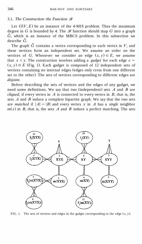
3.1. The Construction]the Function RR

Ž .Let G V, E be an instance of the 4-MIS problem. Thus the maximumdegree in G is bounded by 4. The RR function should map G into a graphG, which is an instance of the MBCS problem. In this subsection we

˜describe G.˜The graph G contains a vertex corresponding to each vertex in V, and

these vertices form an independent set. We assume an order on theŽ .vertices of G. Whenever we consider an edge x, y g E, we assume

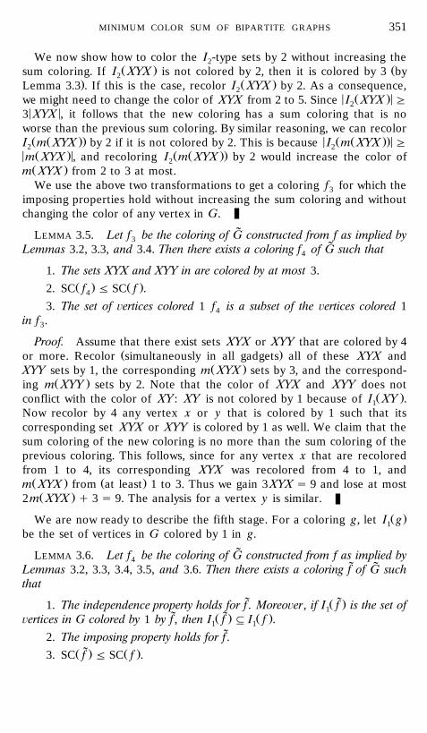
that x - y. The construction involves adding a gadget for each edge e sŽ . Ž .x, y g E Fig. 1 . Each gadget is composed of 12 independent sets of

Žvertices containing no internal edges edges only cross from one different.set to the other . The sets of vertices corresponding to different edges are

disjoint.Before describing the sets of vertices and the edges of any gadget, we

Ž .need some definitions. We say that two independent sets A and B arecliqued, if every vertex in A is connected to every vertex in B, that is, thesets A and B induce a complete bipartite graph. We say that the two sets

< < < <are matched if A s B and every vertex x in A has a single neighborŽ .m x in B, that is, the sets A and B induce a perfect matching. The sets

Ž .FIG. 1. The sets of vertices and edges in the gadget corresponding to the edge x, y .


Ž .and edges in the gadget corresponding to the edge e s x, y are asfollows.

Main and Matched Sets

Ž .1. A set XYX of three vertices and a matched set m XYX of threeŽ .vertices. The sets XYX and m XYX are matched.

Ž .2. A set XYY of three vertices and a matched set m XYY of threeŽ .vertices. The sets XYY and m XYY are matched.

Ž .3. A set XY of six vertices and a matched set m XY of six vertices.Ž .The sets XY and m XY are matched.

Imposing Sets

Ž . Ž .1. A set I XYX of 18 vertices and a set I XYX of 9 vertices. The1 2Ž . Ž .two sets I XYX and I XYX are cliqued.1 2

Ž Ž .. Ž Ž ..2. A set I m XYX of six vertices and a set I m XYX of three1 2Ž Ž .. Ž Ž ..vertices. The sets I m XYX and I m XYX are cliqued.1 2

Ž . Ž Ž ..3. Two sets I XY of 24 vertices and I m XY of 12 vertices.1 1

Additional Edges Between the Sets

1. The vertex x is connected to all three vertices of XYX. The vertexy is connected to all three vertices of XYY.

2. The sets XYX and XY are cliqued. The sets of XYY and XY arecliqued.

Ž . Ž .3. The sets XYX and I XYX are cliqued. The sets m XYX and2Ž Ž ..I m XYX are cliqued.2

Ž . Ž .4. The sets XY and I XY are cliqued. The sets m XY and1Ž Ž ..I m XY are cliqued.1

This completes the description of the gadget corresponding to each edgeŽ .e s x, y and the description of the RR-function. The above sets depend

on e, that is, there is such a gadget for every edge e g E. We avoid addinge as a subscript in these sets, for the simplicity of notation. For the RR

˜function to be valid, we demonstrate a 2 coloring for G, proving that the˜graph G is a bipartite graph.

˜Claim 3.1. The graph G is bipartite.

Proof. Color the independent set corresponding to V, and the six setsŽ . Ž . Ž Ž .. Ž Ž .. Ž .m XYX , m XYY , XY, I m XYX , I m XY and I XYX by 1.1 1 2

˜Color the rest of the vertices in G by 2. Since all of the edges defined


above connect vertices colored by 1 with vertices colored by 2, it follows˜that this is a legal 2-coloring for G.

3.2. The Intuition Behind the Construction

The goal of the construction is to enable us to define the right functionSS . This will be explained in the next subsection. Here we give someintuition.

The role of the imposing sets is to force a situation in which some setscannot be colored by a specific color. For example, it will be shown that in

Ž .an optimal coloring the imposing set I XYX is colored by 2. Conse-2quently, the set XYX cannot be colored by 2. In general, in an optimalsolution, all of the sets of type I are colored by 1, and all of the sets of1type I are colored by 2.2

The role of the matched sets is to ensure that the sum coloring of twomatched sets is fixed in any optimal coloring. For example, if a vertex inXYX is colored by 1, then its matched vertex is colored by 3, and vice versaŽrecalling that these two sets cannot be colored by 2 because of the two

Ž . Ž Ž ...imposing sets I XYX and I m XYX . Thus every pair in XYX and2 2Ž .m XYX adds exactly 4 to the sum coloring in an optimal coloring, and the

Ž .contribution of XYX and m XYX is fixed.Now let us explain the main idea in the construction. Let x and y be

Ž Ž . .two vertices adjacent in G i.e., x, y g E . We will show that we lose inthe sum coloring if both x and y are colored by 1. Indeed, say that both xand y are colored 1, and consider the colors of XY, XYX, XYY. In thebest coloring XYX is colored by 3 and XYY by 2. Therefore, since the setŽ .I XY is colored by 1, it follows that XY is colored by at least 4. On the1

other hand, if one of x and y is not colored by 1, we may gain by assigningXY a color less than 4. This follows since XYX and XYY will ‘‘waste’’ onlyone of the colors 2 and 3. Hence it is possible to color XY with either 2or 3.

Therefore, a ‘‘good’’ sum coloring would color by 1 an independent set inG. In addition, a ‘‘good’’ sum coloring would strive to color as manyvertices of G as possible by 1. It therefore pays to color as large anindependent set as possible in G by 1. Thus a ‘‘good’’ approximationfor the MBCS problem implies a ‘‘good’’ approximation for the 4-MISproblem.

3.3. The Function SS

˜We need the following definition for the construction of SS . A coloring fõf the vertices in G is proper if the two following properties hold for every

edge.


Imposing Properties

Ž . Ž Ž .. Ž . Ž Ž ..1. The sets I XYX , I m XYX , I XY , and I m XY are col-1 1 1 1ored by 1.

Ž . Ž Ž ..2. The sets I XYX and I m XYX are colored by 2.2 2

Independence Property

Ãll of the vertices of G that are colored by 1 in f form an independentset in G.

The process of constructing SS is as follows. We start with any feasible˜coloring f of G. We then show in five stages that f can be transformed to

˜ ã proper coloring f such that the sum of colors in f is no larger than the˜Ž Ž . Ž ..sum of colors in f SC f F SC f . The mapping SS is now defined by

˜choosing the set of vertices in G that are colored by 1 by f , denoted by˜ ˜Ž . Ž .I f . Note that by the independence property, I f is also an indepen-1 1

dent set in G.In the first stage we transform f into f such that all of the vertices in1

any independent set in any gadget are colored by the same color. In thesecond stage, we transform f into a ‘‘locally minimal’’ coloring f . That is1 2a coloring in which each set in the gadget is colored by no more thank q 1, where k is the number of neighboring sets to this set. In the thirdstage, we show how to transform f into a coloring f such that the2 3imposing properties hold. In the fourth stage, we transform f into a3coloring f in which all of the sets XYX and XYY in all of the gadgets are4colored by no more than 3. Finally, in the fifth stage we transform f into3

˜the desired coloring f by showing how to achieve the independenceproperty. In all five stages the new coloring has no worse sum coloring

Ž .than the previous one. Fixing an edge e s x, y , the five stages are statedin Lemmas 3.2, 3.3, 3.4, 3.5, and 3.6.

˜LEMMA 3.2. Let f be a legal coloring of G. Then there exists a coloring f1õf G such that

1. All of the ërtices in any set in the gadget are colored by the samecolor.

Ž . Ž .2. SC f F SC f .1

3. The ërtices corresponding to the ërtices of G are colored the same inboth f and f .1

Proof. Let A be one of the imposing sets in the gadget. Let c be theminimum color of any vertex in the set A. Color all of the vertices in A byc. Since all of the vertices in A are connected in the same fashion to the


vertices outside of A, it follows that this coloring is legal. Let A and B betwo matched sets in the gadget. Let u g A and ¨ g B be two matchedvertices such that the sum of their colors is minimal. Color all of thevertices of A by the color of u and all of the vertices of B by the color of¨ . Since any pair of matched vertices in A and B is connected in the samefashion to the vertices outside A and B, it follows that this coloring islegal. Thus the first property holds. The second property follows, since wedid not increase the sum coloring of any imposing set and any pair ofmatched sets. The third property follows, since we did not touch thevertices of G.

˜LEMMA 3.3. Let f be the coloring of G constructed from f as implied by1Lemma 3.2. Let A be one of the sets in the gadget. Let k be the number of

Žneighboring sets of A. For that purpose, we consider x and y as sets of size 1.˜.For example, if A s YXY, then k s 4. Then there exists a coloring f of G2

such that

1. The color of A is at most k q 1.Ž . Ž .2. SC f F SC f .2

3. All of the properties of f remain.1

Proof. The neighboring sets of A can occupy at most k differentcolors. Hence one color less than or equal k q 1 is legal for A. If A iscolored by a color larger than k q 1, recolor it by this free color. Thus thefirst property holds. The second property follows, since we did not increasethe sum coloring of any set. The third property follows, since we did nottouch the vertices of G.

˜LEMMA 3.4. Let f be the coloring of G constructed from f as implied by2˜Lemmas 3.2 and 3.3. Then there exists a coloring f of G such that3

1. The imposing properties hold for f .3

Ž . Ž .2. SC f F SC f .3

3. All of the properties of f remain.2

Proof. We first show how to color the I -type sets by 1 without1increasing the sum coloring. By Lemma 3.3, we get that the color ofŽ . Ž . Ž .I XYX is at most 3 and the color of I XYX is at most 2. If I XYX is2 1 1

Ž .not colored by 1, then recolor it by 1. In the case where I XYX was2colored by 1, recolor it by the smallest legal color. This smallest color is at

Ž .most 3. This results in a legal coloring in which I XYX is colored by 1.1< Ž . < < Ž . < < Ž . <Since I XYX G 2 I XYX , and since we gained I XYX and lost at1 2 1< Ž . <most 2 I XYX , it follows that the new coloring has a sum coloring that is2

no worse than the previous sum coloring. Similar reasoning shows how toŽ Ž .. Ž . Ž Ž ..color the sets I m XYX , I XY , and I m XY by 1.1 1 1


We now show how to color the I -type sets by 2 without increasing the2Ž . Žsum coloring. If I XYX is not colored by 2, then it is colored by 3 by2

. Ž .Lemma 3.3 . If this is the case, recolor I XYX by 2. As a consequence,2< Ž . <we might need to change the color of XYX from 2 to 5. Since I XYX G2

< <3 XYX , it follows that the new coloring has a sum coloring that is noworse than the previous sum coloring. By similar reasoning, we can recolorŽ Ž .. < Ž Ž .. <I m XYX by 2 if it is not colored by 2. This is because I m XYX G2 2

< Ž . < Ž Ž ..m XYX , and recoloring I m XYX by 2 would increase the color of2Ž .m XYX from 2 to 3 at most.We use the above two transformations to get a coloring f for which the3

imposing properties hold without increasing the sum coloring and withoutchanging the color of any vertex in G.

˜LEMMA 3.5. Let f be the coloring of G constructed from f as implied by3˜Lemmas 3.2, 3.3, and 3.4. Then there exists a coloring f of G such that4

1. The sets XYX and XYY in are colored by at most 3.Ž . Ž .2. SC f F SC f .4

3. The set of ërtices colored 1 f is a subset of the ërtices colored 14in f .3

Proof. Assume that there exist sets XYX or XYY that are colored by 4Ž .or more. Recolor simultaneously in all gadgets all of these XYX and

Ž .XYY sets by 1, the corresponding m XYX sets by 3, and the correspond-Ž .ing m XYY sets by 2. Note that the color of XYX and XYY does not

Ž .conflict with the color of XY: XY is not colored by 1 because of I XY .1Now recolor by 4 any vertex x or y that is colored by 1 such that itscorresponding set XYX or XYY is colored by 1 as well. We claim that thesum coloring of the new coloring is no more than the sum coloring of theprevious coloring. This follows, since for any vertex x that are recoloredfrom 1 to 4, its corresponding XYX was recolored from 4 to 1, andŽ . Ž .m XYX from at least 1 to 3. Thus we gain 3 XYX s 9 and lose at mostŽ .2m XYX q 3 s 9. The analysis for a vertex y is similar.

Ž .We are now ready to describe the fifth stage. For a coloring g, let I g1be the set of vertices in G colored by 1 in g.

˜LEMMA 3.6. Let f be the coloring of G constructed from f as implied by4˜ ˜Lemmas 3.2, 3.3, 3.4, 3.5, and 3.6. Then there exists a coloring f of G such

that

˜ ˜Ž .1. The independence property holds for f. Moreoër, if I f is the set of1˜ ˜Ž . Ž .ërtices in G colored by 1 by f , then I f : I f .1 1

˜2. The imposing property holds for f.˜Ž . Ž .3. SC f F SC f .


Proof. For the independence property, we need to change colors, sothat no two vertices x and y that are adjacent in G are colored by 1.Recall that by Lemma 3.2 all of the vertices in any set are colored by the

Žsame color, and that this color is locally minimal by Lemma 3.3 that is, thecolor of each set is no more than k q 1, if the set have k neighboring

. Ž .sets . We perform the following changes iteratively for every pair ofvertices x and y that are colored by 1 and are adjacent in G.

First note that XYX is colored by 3. This follows, since XYX is notŽ .colored by 1 because of x, is not colored by 2 because of I XYX , and is2

not colored by 4 or more because of Lemma 3.5. We now show how tocolor XYY by 2, without increasing the sum coloring. Suppose that XYY is

Ž . Ž .not colored by 2. Recolor XYY by 2, m XYY by 1, XY by 3, m XY by 2,Ž .XYX by 1, m XYX by 3, and x by 4. Note that we gain at least 3 in the

sum coloring for the recoloring of the vertices in XYY and lose only 3 forrecoloring x. Thus x is no longer colored by 1. Assume now that all of thevertices in XYY are colored by 2. It is now necessarily the case that XY iscolored by at least 4. This is because XY is not colored by 1 because ofŽ .I XY , is not colored by 3 because of XYX, and is not colored by 21

because of XYY. Our final recoloring is as follows. We recolor XY by 3,Ž . Ž . Ž .m XY by 2, XYX by 1, m XYX by 3, XYY by 1, m XYY by 2, and both

x and y by 4. We gain at least 6 for the recoloring of the vertices in XYand lose at most 6 for the recoloring of x and y.

In the transformations described above, we did not increase the sumcoloring. Moreover, the only changes in the colors of vertices in G arefrom color 1 to color 4, proving the first claim of the lemma.

˜ ˜The function SS on any legal coloring f of G is defined as follows. Let fbe the proper coloring constructed from f as implied by Lemmas 3.2, 3.3,

˜ ˜Ž .3.4, 3.5, and 3.6. Let I f be the set of vertices colored by 1 in f. By1Lemma 3.5, this is a feasible independent set. Then

˜SS f s I f .Ž . Ž .1

3.4. The L-Reduction Properties

We now turn to prove the two L-reduction properties. Let OPT be the˜ Ž .minimum sum coloring in G, and let MIC s SC OPT . The next lemma

proves the first property of the L-reduction.

Ž .LEMMA 3.7. There exists a constant a such that MIC F a ? MIS G .

Proof. First note that the degrees in the graph G are at most 4.˜Ž . Ž .Consequently, MIS G G nr5. Also note that G has O n vertices. This is

˜Ž . Ž .because G has O n edges, and G has O 1 additional vertices per any


˜edge in G. Now since G is a bipartite graph and therefore can be coloredŽ .by 1 and 2, it follows that MIC s O n . These two facts imply the first

property.

For the second property of the L-reduction, we need to show the˜existence of a constant b such that for any legal coloring f of G, the

Ž . Ž . Ž Ž . .following holds: MIS G y SS f F b SC f y MIC . We prove thisinequality with b s 1. The proof uses the following two claims. Let I1be the maximum independent set in G.

Claim 3.8. MIC F 135 ? E q 2n y I .1

Proof. Color I by 1 and the rest of the vertices in G by 2. Let1Ž .x, y g E; note that x and y are not both colored by 1, since I is an1independent set. We first color the imposing sets of type I by 1 and the1imposing sets of type I by 2. The contribution of the imposing sets to the2sum coloring per edge is 18 ? 1 q 9 ? 2 q 6 ? 1 q 3 ? 2 q 24 ? 1 q 12 ? 1 s84. Now consider the following three possible cases.

1. Vertex x is colored by 1 and vertex y is colored by 2. Color XYXŽ . Ž . Ž .by 3, m XYX by 1, XYY by 1, m XYY by 2, XY by 2, and m XY by 3.

2. Vertex x is colored by 2 and vertex y is colored by 1. Color XYXŽ . Ž . Ž .by 1, m XYX by 3, XYY by 2, m XYY by 1, XY by 3, and m XY by 2.

Ž .3. Both vertices x and y are colored by 2. Color XYX by 3, m XYXŽ . Ž .by 1, XYY by 1, m XYY by 2, XY by 2, and m XY by 3.

The contribution of all of the matched sets to the sum coloring in all threeŽ . Ž . Ž .cases is 3 1 q 3 q 3 1 q 2 q 6 2 q 3 s 51. Altogether, each gadget in

˜ ˜G contributes 135 to the sum coloring. Since the vertices of G contribute2n y I to the sum, the claim follows.1

˜ Ñow let f be an arbitrary coloring of G and let f be its corresponding˜ ˜Ž .proper coloring. Let I f be the set of vertices colored by 1 in f , and thus1

˜Ž . Ž .SS f s I f .1

˜ ˜Ž . Ž .Claim 3.9. SC f G 135 ? E q 2n y I f .1

˜Proof. Since f is a proper coloring, the contribution of the imposingsets to the sum coloring per edge is 84, as was shown in the previous claim.Now fix an edge and consider the three pairs of matched sets.

Ž . Ž .1. The sets XYX and m XYX contribute at least 3 ? 1 q 3 to thesum coloring. This is because both sets cannot be colored by 2.

Ž . Ž .2. The sets XYY and m XYY contribute at least 3 ? 1 q 2 to thesum coloring. This is because one set must be colored by 2.

Ž . Ž .3. The sets XY and m XY contribute at least 6 ? 2 q 3 to the sumcoloring. This is because both sets cannot be colored by 1.


Altogether, the contribution of the matched sets to the sum coloring peredge is at least 51. The lower bound derived so far is 135 ? E. The claim

˜ ˜Ž . Ž .follows, since the set G _ I f contributes at least 2n y 2 I f to the sum1 1coloring.

Ž . Ž . Ž .LEMMA 3.10. MIS G y SS f F SC f y MIC.

Proof. The following inequalities are implied by Lemma 3.6, Claim 3.8,and Claim 3.9.

˜SC f y MIC G SC f y MICŽ . Ž .˜G 135 ? E q 2n y I f y 135 ? E q 2n y IŽ .Ž .Ž .1 1

s MIS G y SS f .Ž . Ž .

We have completed the construction of a valid L-reduction from the4-MIS problem to the MBCS problem. The following theorem followsfrom Theorems 2.1 and 2.2.

Ž .THEOREM 3.11. There exists an e ) 0 such that there is no 1 q e -ratioapproximation algorithm for the MBCS problem unless P s NP.

4. IMPROVED APPROXIMATION ALGORITHMFOR MBCS

In the previous section we have shown that there exists some e ) 0 suchŽ .that the MBCS problem has no 1 q e -approximation algorithm. How-

ever, the precise threshold for the approximation is yet to be determined.We take a further step in this direction. In this section we present a newalgorithm CC that utilizes a new procedure Neig. We prove that this

Ž . Ž . Ž . Žprocedure, combined with algorithms A 2 , A 3 , and A 4 see Section.2.5 , yields a 10r9-approximation algorithm for the MBCS problem. This

w ximproves the previous 9r8-approximation algorithm of BBH .

4.1. Intuition

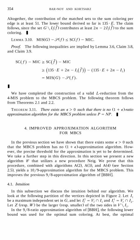
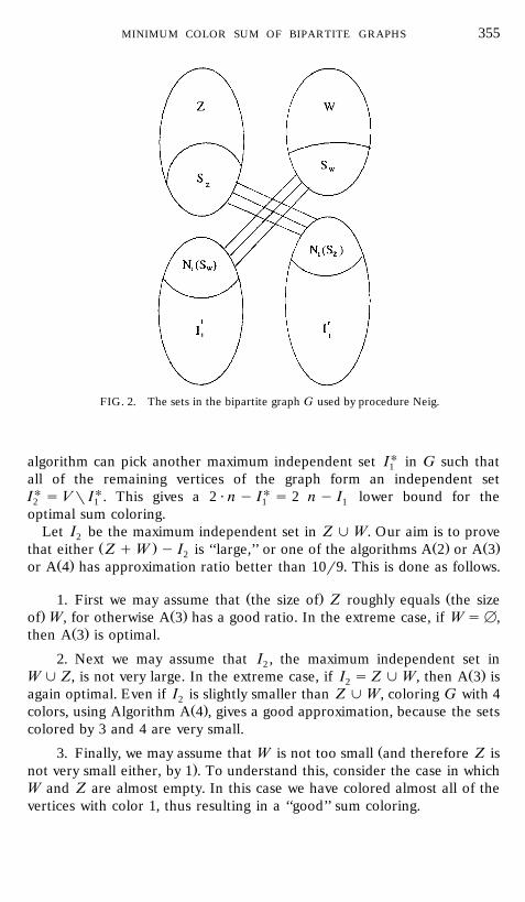
In this subsection we discuss the intuition behind our algorithm. Welook at the following partition of the vertices depicted in Figure 2. Let I1be a maximum independent set in G, and let I 1 s V l I and I 1 s V l I .l l 1 r r 2

Ž . Ž .Let Z resp. W be the larger resp. smaller of the two sides in V _ I .1w xIn the 9r8-ratio approximation algorithm of BBH , the following lower

bound was used for the optimal sum coloring. At best, the optimal


FIG. 2. The sets in the bipartite graph G used by procedure Neig.

algorithm can pick another maximum independent set IU in G such that1all of the remaining vertices of the graph form an independent setIU s V _ IU. This gives a 2 ? n y IU s 2 n y I lower bound for the2 1 1 1optimal sum coloring.

Let I be the maximum independent set in Z j W. Our aim is to prove2Ž . Ž . Ž .that either Z q W y I is ‘‘large,’’ or one of the algorithms A 2 or A 32

Ž .or A 4 has approximation ratio better than 10r9. This is done as follows.

Ž . Ž1. First we may assume that the size of Z roughly equals the size. Ž .of W, for otherwise A 3 has a good ratio. In the extreme case, if W s B,

Ž .then A 3 is optimal.

2. Next we may assume that I , the maximum independent set in2Ž .W j Z, is not very large. In the extreme case, if I s Z j W, then A 3 is2

again optimal. Even if I is slightly smaller than Z j W, coloring G with 42Ž .colors, using Algorithm A 4 , gives a good approximation, because the sets

colored by 3 and 4 are very small.

Ž3. Finally, we may assume that W is not too small and therefore Z is.not very small either, by 1 . To understand this, consider the case in which

W and Z are almost empty. In this case we have colored almost all of thevertices with color 1, thus resulting in a ‘‘good’’ sum coloring.


Ž .Note that 2 and 3 above imply that Z q W y I is large, as required.2This means that there is no ‘‘large’’ independent set in the graph inducedby Z j W. Now, to match the lower bound of 2 ? n y I , many vertices of1Z j W must be colored by 1 in the optimal coloring. Thus our main idea is

Ž .to define a new procedure, Neig, that starts with the coloring of A 3 , usingsome arbitrary maximum independent set I with some corresponding Z1and W, and tries to find a good candidate subset S : Z j W, to berecolored by 1. Note that automatically, all of the neighbors of S need tobe colored by some color other than 1. If such a good set S does not exist,

Ž .it means that we can increase and therefore improve the lower bound2 ? n y I for the optimal coloring.1

Although we are not able to find the best set S to be recolored by 1, wecan find a good ‘‘half’’ of S. Namely, we can find the best set S : W, orWS : Z to be recolored 1, so as to reduce the sum coloring as much asZpossible. Thus we do not choose the best S to move from colors 2 and 3 tocolor 1, but we can choose a subset S or S that reduces the sum by atW Zleast ‘‘half’’ of the reduction in the best choice of S.

4.2. An Algorithmic Tool

We now describe the new tool used in our approximation algorithm.Define the 2-Neighborhood problem as follows. Given a bipartite graphŽ . Ž .G V , V , E , we look for a set S : V such that d s 2S y N S is al r l l S l ll

Ž .maximum. Recall that N S is the set of vertices outside S that have atl lleast one neighbor in S . We note that the order in which V and V arel l rspecified in the problem presentation is important; that is, the solution Slis a subset of V .l

A generalization of this problem, called the proïsion problem, wasw xdiscussed in Chapter 6 of L . In the provision problem, the goal is to

maximize the objective function Ýa x y Ýb y , where x is 1 only if thei i i i irespective vertex in the left side is included, and y is 1 only if theirespective vertex on the right side in included. The restriction in theproblem is that a vertex on the left is included, only if all of its right-sideneighbors are included as well. This problem can be solved by using flowmethods combined with a binary search procedure. The currently fastest

w xalgorithm for the provision problem is given in GGT . For the sake ofcompleteness, we give a brief description of the flow algorithm that solvesour special case of the provision problem}the 2-Neighborhood problem.

We construct the following directed bipartite graph with capacities,Ž .denoted by G9 s V 9, E9 . The set of vertices V 9 contains V and two

additional vertices: a source s and a sink t. The set of edges E9 containsall of the edges in E directed from V to V with capacity `. In addition,l rE9 contains V edges with capacity 1 emanating from s to all of the verticesl


of V , and V edges with capacity 1r2 emanating from all of the vertices inl rV to t.r

We now show how to deduce the solution for the 2-Neighborhoodproblem from a minimum cut in G9. Let V s and V s be the subsets of Vl r land V that are with s in the same side of the minimum cut. Let V t and V t

r l rbe the complementing sets. Note that the cut containing s alone in oneside is finite. Therefore, any vertex in V s is not connected to any vertex inlV t, since otherwise the capacity of the cut is `. Thus the capacity of thercut is given by the following expression: V t q V sr2. The chosen cutl rminimizes this expression, and therefore maximizes the following expres-sion:

V srt s s2 V y V y s 2V y V .l l l rž /2

Since the capacity of the minimum cut is finite, it follows that no vertex inV t has a neighbor in V s. Moreover, every vertex in V s has at least oner l rneighbor in V s, because otherwise moving this vertex to V t would de-l r

s Ž s.crease the capacity of the cut. Therefore, V s N V , which implies thatr lV s is the solution for the 2-Neighborhood problem.l

4.3. Procedure Neig and Algorithm CC

Procedure Neig utilizes the solution to the 2-Neighborhood problemdescribed in Section 4.2. We now define subsets of the vertices of the

Ž .graph G and subgraphs of G used by procedure Neig see Fig. 2 .

1. I }the maximum independent set in G.1

I l s I l V }the left side of I1 1 l 1

I r s I l V }the right side of I .1 1 r 1

2. Z}the larger side of G _ I .1

W}the smaller side of G _ I .1

Without loss of generality, assume that Z ; V and W ; V .l r

Ž r . Ž . r3. G s Z, I , E }the bipartite subgraph induced by Z and I .Z 1 Z 1

Ž l . Ž . lG s W, I , E }the bipartite subgraph induced by W and I .W 1 W 1

Ž .4. S }the set maximizing d s 2S y N S in G .Z S Z Z ZZ

Ž .S }the set maximizing d s 2S y N S in G .W S W W WW

Note that W plays here the role of the left side of the 2-Neighbor-hood problem.

Ž . Ž . r r5. N S s N S l I }the neighbors of S in I .1 Z Z 1 Z 1

Ž . Ž . l lN S s N S l I }the neighbors of S in I .1 W W 1 W 1

Ž . Ž Ž .. Ž .Note that N S N S in G can contain vertices from W Z .Z W


Ž . Ž Ž ..Therefore, we need to define N S N S .1 Z 1 W

Procedure Neig

If d G d : If d - d :S S S SZ W Z Wl r r lŽ Ž .. Ž Ž ..1. Color I j S j I _ N S 1. Color I j S j I _ N S1 Z 1 1 Z 1 W 1 1 Wby 1. by 1.

Ž . Ž .2. Color W j N S by 2. 2. Color Z j N S by 2.1 Z 1 W3. Color Z _ S by 3. 3. Color W _ S by 3.Z W

For the case d G d , procedure Neig can be described as follows.S SZ WŽ . ŽStart with the initial coloring of A 3 , i.e., I is colored by 1, Z the larger1

.of the two remaining sides is colored by 2, and W is colored by 3. ThusŽ Ž .. l rSC A 3 s I q I q 2Z q 3W. Next, recolor Z by 3 and W by 2, losing1 1

Z y W in the sum coloring. Next, change the color of S from 3 to 1,Zgaining 2S in the sum coloring. This forces all of the neighbors of Z inZ

Ž .I , N S , to be colored by a color other than 1, thus color them by 2.1 1 ZŽ .Here we lost N S in the sum coloring. The net profit in the sum1 Z

Ž .coloring is therefore 2S y N S q W y Z s d q W y Z. Similarly, itZ 1 Z SZŽcan be shown that for the case d ) d , the net profit is d . This caseS S SW Z W

is better for us, since we do not need to switch the colors of Z and W,.losing Z y W. Thus we proved the following proposition.

Ž . Ž . Ž Ž ..PROPOSITION 4.1. 1 If d G d , then SC Neigh s SC A 3 yS SZ WŽ .d q Z y W .SZ

Ž . Ž . Ž Ž ..2 If d ) d , then SC Neig s SC A 3 y d .S S SW Z W

We conclude this subsection with the description of Algorithm CC. Itclearly follows that the algorithm has a polynomial running time.

Algorithm CC

Ž . Ž . Ž .v Run algorithms A 2 , A 3 , A 4 , and procedure Neig.v Pick the solution whose sum coloring is the minimum among the

four coloring solutions.

4.4. Analysis

In this subsection we analyze the approximation ratio of Algorithm CC.Ž . Ž .All through the analysis, let Z s n y I r2 q e n and W s n y I r21 d 1

y e n. The term e n quantifies the extent to which the graph induced byd dZ j W is unbalanced. This is the resulting graph once the maximumindependent set I is deleted from G.1


Outline of the Analysis

� Ž Ž ..v If Z y W s 2e n is ‘‘large’’ enough, then already min SC A 2 ,dŽ Ž ..4SC A 3 yields the 10r9-ratio.

v Otherwise, Z y W is not too ‘‘large.’’ If I is ‘‘large’’ enough, then2� Ž Ž .. Ž Ž ..4this time already min SC A 2 , SC A 4 yields the 10r9-ratio.

v Otherwise, W is almost as ‘‘large’’ as Z and I is not too ‘‘large.’’ If2W is ‘‘small’’ enough and therefore Z is also ‘‘small’’ and I is ‘‘large’’1

Ž Ž ..enough, then SC A 3 alone yields the 10r9-ratio.v Otherwise Z y W and I are not too ‘‘large’’ and W is not too2

‘‘small.’’ If the optimal algorithm does not deviate much from algorithmŽ . � Ž Ž .. Ž Ž ..4A 3 , then again min SC A 2 , SC A 3 yields the 10r9-ratio.

v Finally, if all of the previous conditions do not hold, we use the new� Ž Ž .. Ž .4procedure Neig and show that min SC A 2 , SC Neig yields the 10r9-

ratio.

The analysis is therefore partitioned into five cases. In each case, we makesome assumption A, proving that under this assumption, the 10r9-ratio isguaranteed. We therefore continue the analysis assuming that A does nothold.

Case 4.2. e G 1r40.dIn this case, consider the performance of the best of the two algorithmsŽ . Ž . Ž Ž .. Ž . Ž .A 2 and A 3 . Clearly, SC A 2 F 3nr2 see Section 2.5 . Algorithm A 3

colors I by 1, Z by 2, and W by 3. Hence,1

SC A 3 s I q 2Z q 3WŽ .Ž . 1

5n y 3I1s y e nd2

5n y 3I1F y nr40.2

On the other hand, the optimal coloring, OPT, colors at most I vertices1Ž .by 1 and the rest of the vertices by at least 2. This implies that SC OPT G

Ž Ž .. Ž .2n y I . It follows that SC A 3 rSC OPT increases when I decreases.1 1Ž Ž .. Ž Ž ..Therefore, the worst case for Algorithm CC is when SC A 2 s SC A 3

Ž .s 3nr2. We get 3nr2 s 5n y 3I r2 y nr40, which implies that I s1 1Ž .13nr20. For this value of I the lower bound for SC OPT is 27nr20. The1

10r9 bound follows, since

SC CC 3nr2 10Ž .F s .

SC OPT 27nr20 9Ž .Hence we may continue the analysis under the following assumption.


ASSUMPTION 4.3. e F 1r40. Let e s 1r40 y e .d d

W 2eCase 4.4. I G Z q q n.2 3 3We prove here, in a proof similar to Case 4.2, that the best of Algo-

Ž . Ž . Ž .rithms A 2 and A 4 always has a 10r9-ratio. Algorithm A 4 has thefollowing properties. It colors I by 1, I by 2, at least half of the re-1 2

Ž .maining n y I y I vertices by 3, and the rest of the vertices by 4. The1 2Ž .worst case for A 4 is when I is minimal; in this case it happens when2Ž .I s Z q Wr3 q 2e n r3. This gives the following upper bound:2

n y I y I n y I y I1 2 1 2SC A 4 F I q 2 I q 3 q 4Ž .Ž . 1 2 ž / ž /2 2

W 2e n W e n W e nF I q 2 Z q q q 3 y q 4 y1 ž / ž / ž /3 3 3 3 3 3

s I q 2Z q 3W y e n1

5n y 3I1s y e q e nŽ .d2

5n y 3I n1s y .2 40

The 10r9-ratio follows as in Case 4.2, where again we choose the bestŽ .between two algorithms, one with SC s 5n y 3I r2 y nr40 and one1

with SC s 3nr2.

W 2eASSUMPTION 4.5. I F Z q q n.2 3 3

Ž .Case 4.6. W F 5e n q 6e n.dŽ .In this case we consider only the performance of Algorithm A 3 . Recall

Ž Ž .. Ž .that SC A 3 s I q 2Z q 3W, while SC OPT G 2n y I . Therefore,1 1

SC A 3 I q 2Z q 3WŽ .Ž . 1FSC OPT 2n y IŽ . 1

Ws 1 q

n q Z q W

Ws 1 q

n q 2W q 2e nd


WF 1 q max ½ 5n q 2W q 2e nW d

5e q 6edF 1 q .1 q 10e q 14ed

The last inequality follows, since the expression increases with W, and inŽ . Ž .this case W is bounded by 5e q 6e n. Since e s 1r40 y e , it followsd d

that

SC A 3 1r8 q e 6r40 10Ž .Ž . dF 1 q F 1 q s .SC OPT 1 q 1r4 q 4e 1 q 14r40 9Ž . d

The last inequality follows, since the expression increases with e andde F 1r40 by Assumption 4.3.d

Ž .ASSUMPTION 4.7. W G 5e q 6e n.dBefore dealing with the fourth case, we need to prove some claims. The

following corollary is derived directly from Assumptions 4.5 and 4.7.

8eCOROLLARY 4.8. Z q W y I G q 4e n.2 dž /3

Note the implication of Corollary 4.8. Suppose that the number ofvertices colored by 2 in OPT roughly equals I . Then since OPT cannot2color more than I vertices by 1, the corollary indicates that roughly1Z q W y I vertices in OPT are colored by at least 3. Keeping this in2mind, we make the following definitions. Let IU be the set of vertices1colored by 1 in OPT. Let A be the set of vertices from Z j W that are

U Ž .colored by 1 in OPT. That is, A s I l Z j W . Note that the set1Ž . Ž .N A s N A l I is thus not colored by 1 in OPT. More precisely, the1 1

Žset of vertices not colored by 1 in OPT, denoted by ALT , equals Z jŽ ..W j N A _ A. The next claim states that the maximum independent set,1

Ž .MIS ALT , in the graph induced by ALT is ‘‘small enough.’’ The corollarythat follows the claim indicates that ‘‘many’’ of the vertices of ALT arecolored by at least 3.

Ž . ŽŽ Ž .. .Claim 4.9. MIS ALT s MIS Z j W j N A _ A F Z q W y1Ž . Ž .8er3 q 4e n q N A .d 1

ŽŽ Ž .. . ŽŽ Ž ..Proof. We have MIS Z j W j N A _ A F MIS Z j W j N A1 1Ž . Ž .F MIS Z j W q N A . Now the desired inequality follows from Corol-1

Ž .lary 4.8, since MIS Z j W s I .2

Ž .COROLLARY 4.10. In OPT, exactly I y N A q A ërtices are colored1 1Ž .by 1, and at least 8er3 q 4e n y A ërtices are colored by 3.d


Proof. The first part of the claim is by definition. To prove the secondpart of the corollary, note that the number of vertices outside IU is1Ž Ž . .Z q W q N A y A and that the bound on the independent set of1

U Ž Ž . Ž ..G _ I is Z q W y 8er3 q 4e n q N A . Subtracting these two ex-1 d 1Ž .pressions gives 8er3 q 4e n y A.d

Thus the following bound on the optimal sum is derived.

8eSC OPT G I y N A q A q 2 Z q W y q 4e n q N AŽ . Ž . Ž .Ž .1 1 d 1ž /ž /3

8eq 3 q 4e n y Adž /ž /3

8es 2n y I y 2 A y N A q q 4e n. 1Ž . Ž .Ž .1 1 dž /3

We are now ready to deal with the fourth case.

Ž . Ž .Case 4.11. 2 A y N A F 2e q 4e n.1 dŽ .Plugging this upper bound into inequality 1 gives

2e nSC OPT G 2n y I q . 2Ž . Ž .1 3

Ž .Recall that the usual lower bound on SC OPT is 2n y I , and thus this1lower bound is an improvement. As in Case 4.2, we consider the perfor-

Ž . Ž .mance of the best of the two algorithms A 2 and A 3 . It turns out thatŽ .the ratio A 3 increases when I decreases. Hence the worst case is when1

Ž Ž .. Ž Ž .. Ž .SC A 2 s SC A 3 s 3nr2. We get 3nr2 s 5n y 3I r2 y e n, which1 dŽ . Ž .implies that I s 2r3 y 2e r3 n. By inequality 2 we get that1 d

2e n 4n 2 1r40 n 27nŽ .SC OPT G 2n y I q s q s .Ž . 1 3 3 3 20

The 10r9 bound follows as in Case 4.2.

Ž . Ž .ASSUMPTION 4.12. 2 A y N A G 2e q 4e n.1 dWe are now ready to complete the analysis of Algorithm CC. The next

case is the remaining case.

Case 4.13. We now show that under Assumptions 4.3, 4.5, 4.7, and 4.12it is enough to consider the combined performance of procedure Neig and

Ž . U Ž .Algorithm A 2 . Recall that A s I l Z j W is the subset of Z j W1Ž .that is colored by 1 in OPT. Let A s Z l A, A s W l A, N A sZ W 1 Z

Ž . Ž . Ž .N A l I , and N A s N A l I . It follows from Assumption 4.12Z 1 1 W W 1Ž . Ž . Ž . Ž .that either 2 A y N A G e q 2e n or 2 A y N A G e q 2e n.Z 1 Z d W 1 W d


Ž .Consequently, either d or d is greater or equal to e q 2e n. This isS S dZ W

because procedure Neig finds the sets that maximize expressions of theŽ .form 2S y N S .

Ž .The worst case happens when only d G e q 2e n. This is becauseS dZŽ . Žotherwise the gain of procedure Neig over Algorithm A 3 is larger see

.Proposition 4.1 . Hence, by Proposition 4.1,

SC Neig s SC A 3 q Z y W y dŽ . Ž . Ž .Ž . SZ

5n y 3I1F y e n q 2e n y e q 2e nŽ .d d d2

5n y 3I1s y e q e nŽ .d2

5n y 3I n1s y .2 40

Ž .Thus, as in Case 4.2, the best of procedure Neig and Algorithm A 2 yieldsthe 10r9-ratio. We have completed the proof of the following theorem.

THEOREM 4.14. Algorithm CC is a polynomial 10r9-approximation algo-rithm for the MBCS problem.

5. DISCUSSION AND FUTURE WORK

We have proved that the MBCS is NP-hard and, furthermore, admits nopolynomial time approximation scheme, unless P s NP. We have alsogiven an improved 10r9-ratio approximation algorithm for MBCS.

The following are two open problems related to our work:

v Determine the best constant-ratio approximation for MBCS. Is the10r9-ratio algorithm the best possible? A good direction in which to lookis the following: Is it possible to choose a better set S to be removed fromZ j W and be recolored by 1 in Neig? Note that our algorithm recolors by

Ž1 a set S or S that is entirely contained in a single side left side or rightW Z. Ž .side . It may be possible to gain more by recoloring an independent set S

containing vertices of both Z and W.v Give good approximation algorithms for MCS on other families of

graphs, such as interval graphs. An important contribution was made inw xthat respect in NSS , where a ratio 2 algorithm was presented for MCS on

interval graphs. Can this ratio be improved? Furthermore, no MAXSNP-hardness result is known for MCS on interval graphs.


REFERENCES

w xALM S. Arora, C. Lund, R. Motwani, M. Sudan, and M. Szegedy, Proof verification andintractability of approximation problems, in ‘‘Proc. of the 33rd IEEE Symp. Founda-tions Computer Science,’’ pp. 14]23, 1992.

w xAS B. Awerbuch and M. Saks, A dining philosophers algorithm with polynomialresponse time, in ‘‘Proc. 31st IEEE Symp. Foundation Computer Science,’’ pp.65]74, 1990.

w xBP J. Bar-Ilan and D. Peleg, Distributed resource allocation algorithms, in ‘‘Proc. SixthInternational Workshop Distributed Algorithms,’’ pp. 276]291, 1992.

w xBBH A. Bar-Noy, M. Bellare, M. M. Halldorsson, H. Shachnai and T. Tamir, Onćhromatic sums and distributed resource allocation, Information and Computation

Ž .140 1998 , 183]202.w xBF P. Berman and M. Furer, Approximating maximum independent set in bounded¨

degree graphs, in ‘‘Proc. Fifth ACM-SIAM Symp. Discrete Algorithms,’’ pp. 365]371,1994.

w xBCC A. Blum, P. Chalasani, D. Coppersmith, B. Pulleyblank, P. Raghavan, and M.Sudan. The minimum latency problem, in ‘‘Proc. 26th IEEE Symp. Theory Comput-ing,’’ pp. 163]171, 1994.

w xCM K. Chandy and J. Misra, The drinking philosophers problems, ACM Trans. Pro-Ž .gramming Languages Syst. 6 1984 , 632]646.

w xChr N. Christofides, Worst case analysis of a new heuristic for the traveling salesmanproblem, Tech. Rep. GSIA, Carnegie-Mellon Univ., Pittsburgh, 1976.

w x Ž .E P. Erdos, On the graph-theorem of Turan, Math. Lapok, 21 1970 , 249]251.¨ ´w xEKS P. Erdos, E. Kubicka, and A. J. Schwenk, Graphs that require many colors to¨

Ž .achieve their chromatic sum, Congr. Numer. 71 1990 , 17]28.w xFK U. Feige and J. Kilian, Zero knowledge and the chromatic number, in ‘‘Proc. 11th

IEEE Conf. Computational Theory,’’ pp. 278]287, 1996.w xGGT G. Gallo, M. D. Grigoriadis, and R. E. Tarjan, A fast parametric maximum flow

Ž .algorithm and applications, SIAM J. Comput. 18 1989 , 30]55.w x 1y eHas J. Hastad, Clique is hard to approximate within n , in ‘‘Proc. 37th IEEE Symp.˚

Foundation Computer Sci.,’’ pp. 627]639, 1996.w xH D. S. Hochbaum, Efficient bounds for the stable set, vertex cover and set packing

Ž .problems, Discrete Appl. Math. 6 1983 , 243]254.w xHR M. M. Halldorsson and J. Radhakrishnan, Greed is good: Approximating indepen-´

dent sets in sparse and bounded-degree graphs, in ‘‘Proc. 26th IEEE Symp. TheoryComputing,’’ pp. 439]448, 1994.

w xK E. Kubicka, ‘‘The Chromatic Sum of a Graph,’’ Ph.D. Thesis, Western MichiganUniversity, Kalamazoo, MI, 1989.

w xKKK E. Kubicka, G. Kubicki, and D. Kountanis, Approximation algorithms for thechromatic sum, in ‘‘Proc. First Great Lakes Computer Sci. Conf.,’’ Springer LNCS507, pp. 15]21, 1989.

w xKS E. Kubicka and A. J. Schwenk, An introduction to chromatic sums, in ‘‘Proc. ACMComputer Sci. Conf.,’’ pp. 39]45, 1989.

w xL E. Lawler, ‘‘Combinatorial Optimization Networks and Matroids,’’ Holt, Rinehartand Winston, New York, 1976.


w xLYN N. Lynch, Upper bounds for static resource allocation in a distributed system,Ž .J. Comput. System Sci. 23 1981 , 254]278.

w xNSS S. Nicoloso, M. Sarrafzadeh, and X. Song. On the sum coloring problem on intervalgraphs, unpublished manuscript.

w xPY C. H. Papadimitriou and M. Yannakakis, Optimization approximation and complex-ity classes, in ‘‘Proc. 20th IEEE Symp. Theory Computing, pp. 229]234, 1988.

w x Ž .T P. Turan, An external problem in graph theory, Mat. Fiz Lapok 48 1941 , 436]452.´w xTEA C. Thomassen, P. Erdos, Y. Alavi, J. Malde, and A. J. Schwenk, Tight bounds on the¨

Ž .chromatic sum of a connected graph, J. Graph Theory 13 1989 , 353]357.

Documents

Minimum Color Sum of Bipartite Graphs