MINIMUM SYMBOL ERROR RATE TIMING RECOVERY SYSTEM

by

Nagendra Bage Jayaraj

A thesis submitted in partial fulfillmentof the requirements for the degree

of

MASTER OF SCIENCE

in

Electrical Engineering

Approved:

Dr. Jacob Gunther Dr. Todd MoonMajor Professor Committee Member

Dr. Edmund Spencer Dr. Byron R. BurnhamCommittee Member Dean of Graduate Studies

UTAH STATE UNIVERSITYLogan, Utah

2010

ii

Copyright c© Nagendra Bage Jayaraj 2010

All Rights Reserved

iii

Abstract

Minimum Symbol Error Rate Timing Recovery System

by

Nagendra Bage Jayaraj, Master of Science

Utah State University, 2010

Major Professor: Dr. Jacob GuntherDepartment: Electrical and Computer Engineering

This thesis presents a timing error detector (TED) used in the symbol timing synchro-

nization subsystem for digital communications. The new timing error detector is designed

to minimize the probability of symbol decision error, and it is called minimum symbol error

rate TED (MSERTED). The new TED resembles the TED derived using the maximum

likelihood (ML) criterion but gives rise to faster convergence relative to MLTED. The new

TED requires shorter training sequences for symbol timing recovery. The TED operates

on the outputs of the matched filter and estimates the timing offset. The S-curve is used

as a tool for analyzing the behavior of the TEDs. The faster convergence of the new TED

is shown in simulation results as compared to MLTED. The new TED works well for any

two-dimensional constellation with arbitrarily shaped decision regions.

(44 pages)

iv

To my beloved family, friends, and my soul Parinita.

v

Acknowledgments

This research project would have never been completed without my advisor and mentor,

Dr. Jacob Gunther. This project is the outcome of his constant motivation and belief in me.

I would have never been able to complete this research without his guidance, patience, and

expertise in the field of digital signal processing (DSP) and communications. His courses

provided the foundation for my research and helped me become a better researcher. I am

grateful, and thank him for all his guidance, support, and valuable time. I would also like

to thank my committee members, Dr. Todd Moon and Dr. Edmund Spencer, for extending

their support.

Also, I would like to thank my father, P Jayaraj, who has been always supporting me

in whatever I do; and my mother, Uma Jayaraj, who has been the inspiration in my life.

I would like to thank my sister, Bhavya, and brother-in-law, Hrishikesh, who have always

given me the moral support at critical times. I would like to thank my niece, Parinita, who

is very special to me. She is the one who brings a smile to my face. I would like to thank

Dr. David Hailey and Dr. Chris Hailey for their support during my stay at USU. Finally, I

would like to acknowledge my friends, especially Reddy, Loki, Shantha, Balu, Koli, Barey,

Dharnish, Kiran, Atul, Karthik, Amrita, Chandu, Kalyan, Pradeep, Hema Swaroop, Rahul,

and Nagaravind, with whom I have spent the best times of my student life.

Nagendra Bage Jayaraj

vi

Contents

Page

Abstract . . . . . . . . . . . . . . . . . . . . . . . . . . . . . . . . . . . . . . . . . . . . . . . . . . . . . . . iii

Acknowledgments . . . . . . . . . . . . . . . . . . . . . . . . . . . . . . . . . . . . . . . . . . . . . . . v

List of Figures . . . . . . . . . . . . . . . . . . . . . . . . . . . . . . . . . . . . . . . . . . . . . . . . . . vii

1 Introduction . . . . . . . . . . . . . . . . . . . . . . . . . . . . . . . . . . . . . . . . . . . . . . . . . 1

2 Datamodel . . . . . . . . . . . . . . . . . . . . . . . . . . . . . . . . . . . . . . . . . . . . . . . . . . . 5

2.1 Datamodel . . . . . . . . . . . . . . . . . . . . . . . . . . . . . . . . . . . . 52.2 Probability of Error . . . . . . . . . . . . . . . . . . . . . . . . . . . . . . . 72.3 S-Curves . . . . . . . . . . . . . . . . . . . . . . . . . . . . . . . . . . . . . . 11

3 Implementation . . . . . . . . . . . . . . . . . . . . . . . . . . . . . . . . . . . . . . . . . . . . . . . 17

3.1 Transmitter Processing . . . . . . . . . . . . . . . . . . . . . . . . . . . . . . 173.2 Receiver Processing . . . . . . . . . . . . . . . . . . . . . . . . . . . . . . . . 17

4 Results . . . . . . . . . . . . . . . . . . . . . . . . . . . . . . . . . . . . . . . . . . . . . . . . . . . . . . 21

4.1 Probability of Error . . . . . . . . . . . . . . . . . . . . . . . . . . . . . . . 214.2 Symbol Error Rate . . . . . . . . . . . . . . . . . . . . . . . . . . . . . . . . 214.3 Error Signal Plots . . . . . . . . . . . . . . . . . . . . . . . . . . . . . . . . 234.4 Clock Frequency Offset . . . . . . . . . . . . . . . . . . . . . . . . . . . . . . 29

5 Conclusion and Future Work . . . . . . . . . . . . . . . . . . . . . . . . . . . . . . . . . . . . 30

5.1 Conclusion . . . . . . . . . . . . . . . . . . . . . . . . . . . . . . . . . . . . 305.2 Future Work . . . . . . . . . . . . . . . . . . . . . . . . . . . . . . . . . . . 30

References . . . . . . . . . . . . . . . . . . . . . . . . . . . . . . . . . . . . . . . . . . . . . . . . . . . . . . 32

Appendix . . . . . . . . . . . . . . . . . . . . . . . . . . . . . . . . . . . . . . . . . . . . . . . . . . . . . . 34

vii

List of Figures

Figure Page

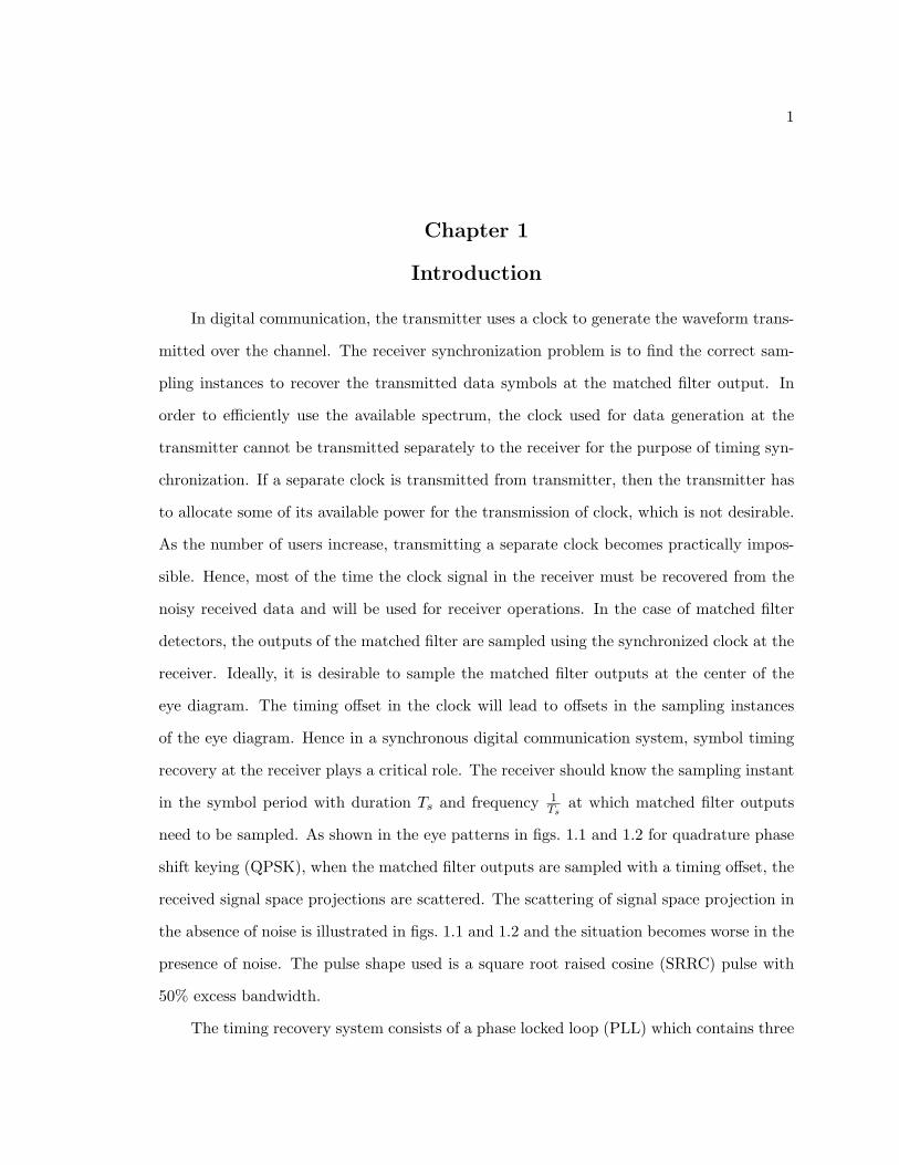
1.1 Scatter plot with timing offset of 0.5Ts in the absence of noise. . . . . . . . 2

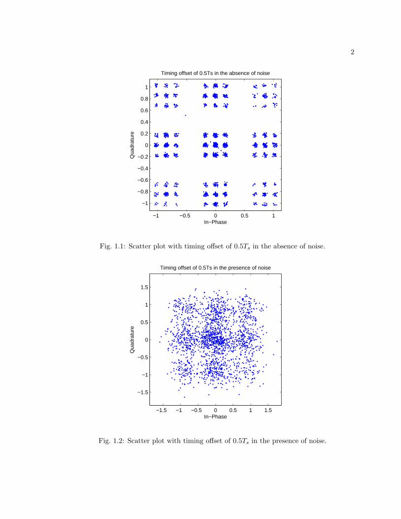
1.2 Scatter plot with timing offset of 0.5Ts in the presence of noise. . . . . . . . 2

2.1 16-quadrature amplitude modulation (QAM) constellation. . . . . . . . . . 10

2.2 S-curves at -10 dB and 0 dB. . . . . . . . . . . . . . . . . . . . . . . . . . . 13

2.3 S-curves at 2.5 dB and 5 dB. . . . . . . . . . . . . . . . . . . . . . . . . . . 13

2.4 S-curves at 8 dB and 10 dB. . . . . . . . . . . . . . . . . . . . . . . . . . . . 14

2.5 S-curves at 15 dB. . . . . . . . . . . . . . . . . . . . . . . . . . . . . . . . . 14

2.6 Normalized S-curves at -10 dB and 0 dB. . . . . . . . . . . . . . . . . . . . 15

2.7 Normalized S-curves at 2.5 dB and 5 dB. . . . . . . . . . . . . . . . . . . . 15

2.8 Normalized S-curves at 8 dB and 10 dB. . . . . . . . . . . . . . . . . . . . . 16

2.9 Normalized S-curves at 15dB. . . . . . . . . . . . . . . . . . . . . . . . . . . 16

3.1 Transmitter processing. . . . . . . . . . . . . . . . . . . . . . . . . . . . . . 18

3.2 Receiver processing. . . . . . . . . . . . . . . . . . . . . . . . . . . . . . . . 19

3.3 Farrow Interpolator. . . . . . . . . . . . . . . . . . . . . . . . . . . . . . . . 20

4.1 Log-probability of error at various SNRs. . . . . . . . . . . . . . . . . . . . 22

4.2 Symbol error rates at -10 dB and 0 dB. . . . . . . . . . . . . . . . . . . . . 24

4.3 Symbol error rates at 2.5 dB and 5 dB. . . . . . . . . . . . . . . . . . . . . 24

4.4 Symbol error rates at 8 dB and 10 dB. . . . . . . . . . . . . . . . . . . . . . 25

4.5 Symbol error rate at 15 dB. . . . . . . . . . . . . . . . . . . . . . . . . . . . 25

4.6 Symbol error rates at 8 dB and 10 dB for τ = 0.25Ts. . . . . . . . . . . . . 26

4.7 Error signals at -10 dB and 0 dB. . . . . . . . . . . . . . . . . . . . . . . . . 26

viii

4.8 Error signals at 2.5 dB and 5 dB. . . . . . . . . . . . . . . . . . . . . . . . . 27

4.9 Error signals at 8 dB and 10 dB. . . . . . . . . . . . . . . . . . . . . . . . . 27

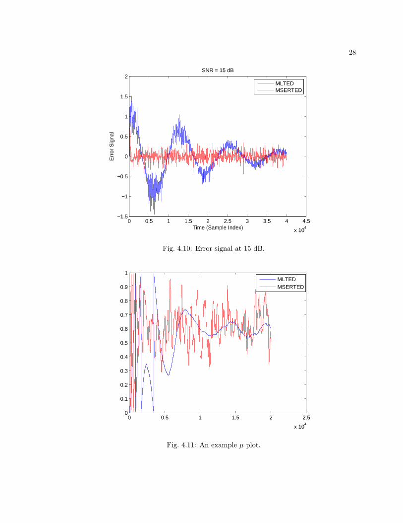
4.10 Error signal at 15 dB. . . . . . . . . . . . . . . . . . . . . . . . . . . . . . . 28

4.11 An example µ plot. . . . . . . . . . . . . . . . . . . . . . . . . . . . . . . . . 28

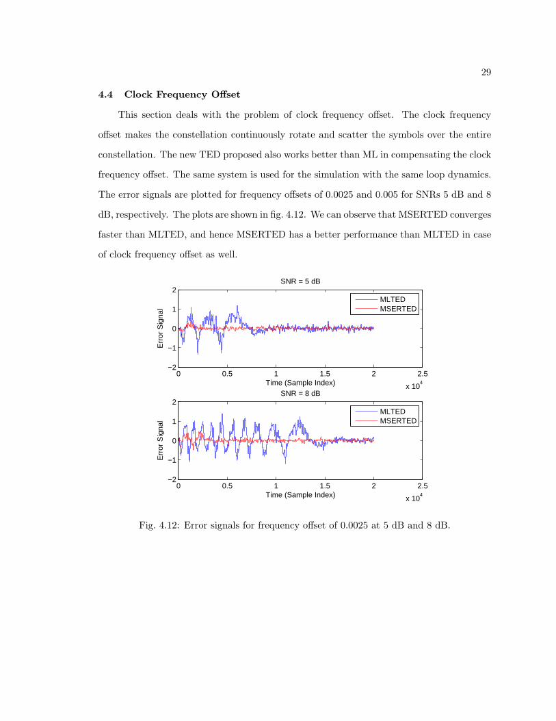
4.12 Error signals for frequency offset of 0.0025 at 5 dB and 8 dB. . . . . . . . . 29

1

Chapter 1

Introduction

In digital communication, the transmitter uses a clock to generate the waveform trans-

mitted over the channel. The receiver synchronization problem is to find the correct sam-

pling instances to recover the transmitted data symbols at the matched filter output. In

order to efficiently use the available spectrum, the clock used for data generation at the

transmitter cannot be transmitted separately to the receiver for the purpose of timing syn-

chronization. If a separate clock is transmitted from transmitter, then the transmitter has

to allocate some of its available power for the transmission of clock, which is not desirable.

As the number of users increase, transmitting a separate clock becomes practically impos-

sible. Hence, most of the time the clock signal in the receiver must be recovered from the

noisy received data and will be used for receiver operations. In the case of matched filter

detectors, the outputs of the matched filter are sampled using the synchronized clock at the

receiver. Ideally, it is desirable to sample the matched filter outputs at the center of the

eye diagram. The timing offset in the clock will lead to offsets in the sampling instances

of the eye diagram. Hence in a synchronous digital communication system, symbol timing

recovery at the receiver plays a critical role. The receiver should know the sampling instant

in the symbol period with duration Ts and frequency 1Ts

at which matched filter outputs

need to be sampled. As shown in the eye patterns in figs. 1.1 and 1.2 for quadrature phase

shift keying (QPSK), when the matched filter outputs are sampled with a timing offset, the

received signal space projections are scattered. The scattering of signal space projection in

the absence of noise is illustrated in figs. 1.1 and 1.2 and the situation becomes worse in the

presence of noise. The pulse shape used is a square root raised cosine (SRRC) pulse with

50% excess bandwidth.

The timing recovery system consists of a phase locked loop (PLL) which contains three

2

−1 −0.5 0 0.5 1

−1

−0.8

−0.6

−0.4

−0.2

0

0.2

0.4

0.6

0.8

1

Qua

drat

ure

In−Phase

Timing offset of 0.5Ts in the absence of noise

Fig. 1.1: Scatter plot with timing offset of 0.5Ts in the absence of noise.

−1.5 −1 −0.5 0 0.5 1 1.5

−1.5

−1

−0.5

0

0.5

1

1.5

Qua

drat

ure

In−Phase

Timing offset of 0.5Ts in the presence of noise

Fig. 1.2: Scatter plot with timing offset of 0.5Ts in the presence of noise.

3

components: a timing error detector (TED), a loop filter and an interpolator controlled by

an interpolation control block. The timing error detector outputs the error signal e which

is related to the difference between the unknown timing offset τ and the estimate of the

timing offset τ . The PLL adjusts the estimate τ to be close to the timing offset τ and forces

the error signal to be zero.

A widely used optimization criterion in deriving the timing and phase recovery sys-

tems is the maximum likelihood (ML) criterion [1, 2]. The problem of carrier phase and

symbol timing recovery for baseband pulse amplitude modulation (PAM) was examined

by Franks [3]. Meyers and Franks [4] explored the problem of symbol timing and car-

rier phase estimation for PAM using both data-aided (DA) estimators and nondata-aided

(NDA) estimators. The log-likelihood ratio L is differentiated with respect to τe to obtain

the error signal and the equation dLdτe

= 0 is solved by the PLL. In case of MSER, the

logarithm of probability of error is used as the criterion to obtain the error signal used for

the synchronization.

The probability of error criterion is widely used as an alternative to the traditional

mean-squared approaches for addressing the digital communications problems. Gunther

and Moon [5] use this approach to derive the minimum symbol error rate phase recovery

system. Aaron and Tufts [6] showed that the average minimum probability of error receiver

for binary PAM transmitted through a noisy and dispersive medium consists of a linear

filter which is the matched filter itself followed by a tapped delay line. Yen [7] and Chen et

al. [8] derive decision feedback equalizers using the minimum error rate probability condition

along with the use of stochastic gradient approach. It is also pointed out that, in general,

MSER algorithms work well and are never trapped at locally minimizing solutions. Gunther

and Moon [9] use Bayes risk in deriving the minimum Bayes risk adaptive linear equalizers

which can be applied to any two-dimensional constellations with arbitrarily shaped decision

regions. Yeh and Barry [10, 11] use error probability to derive adaptive linear equalizers.

Yeh et al. [12], Chen et al. [13], Wang et al. [14], and Psaromiligkos et al. [15] investigate

minimum bit error rate multi-user detection. Minimum bit error rate beamformers in a

4

multi-antenna communication scenario were developed by Chen et al. [16] and Samir et

al. [17]. Most of the prior work centers on the M-ary quadrature amplitude modulation

(QAM) where the decision boundaries are rectangular. But in case of MSERTED, the

two-dimensional constellations can have arbitrarily shaped decision regions.

The maximum likelihood timing error detector (MLTED) uses the slope of the eye

diagram to produce the error signal. There exist two flavors of MLTED, namely the data-

aided case and the nondata-aided case. A more general class of data aided MLTED was

developed by Bergmans and Wong [18]. The early-late timing error detector (ELTED)

approximates the derivative required by MLTED using time differences. The zero-crossing

timing error detector (ZCTED) works on the zero crossings of the eye diagram. It operates

at two samples/symbol on the matched filter outputs. The Gardner timing error detector

(GTED) was developed by Gardner [19]. The algorithm was intended for synchronous

binary phase shift keying (BPSK) and QPSK. The GTED is not decision directed and the

clock recovery is independent of carrier phase recovery. Mueller an Muller [20] developed a

TED called Mueller-Muller TED (MMTED) which operates at one sample/symbol period

and convergence is exponential. One of the important performance evaluation parameters

of these TEDs is the self noise. MLTED and ELTED have more self noise when compared

to ZCTED, GTED, and MMTED. The MSERTED has higher self noise than MLTED.

This thesis is organized in the following manner. Chapter 2 presents the data model

and probability of error modeling along with the S-curves which are used as a tool for the

analysis of the new TED. Chapter 3 discusses the implementation of the timing recovery sys-

tem. Chapter 4 discusses the performance of MSERTED against MLTED using simulation

results. Finally, Chapter 5 concludes the thesis and suggests some future work.

5

Chapter 2

Datamodel

2.1 Datamodel

This chapter describes the datamodel and the probability of error modeling used to

derive the MSERTED. The S-curves are derived to gain an insight on the behavior of the

MSERTED as compared to MLTED.

Let A = {c1, c2, · · · , cM},M = 2b, define a constellation of complex symbols, (i.e.,

ci ∈ C for all i). A transmitter randomly selects symbols a (n) ∈ A and transmits them

over an intersymbol interference (ISI) channel at a rate of 1/Ts symbols per second.

The received signal at the matched filter input is:

r (t) = G∑

n

a (n) p (t− nTs − τ) + u (t) , (2.1)

where a (n) ∈ constellation A, G is the composite of all the amplitude gains and losses

occurred during transmission, p (t) is the square root raised cosine (SRRC) pulse with unit

energy and support in the interval −LpTs ≤ t ≤ LpTs, τ is the unknown timing delay, u (t)

is white Gaussian noise with variance σ2.

The received signal is passed through the matched filter with impulse response p (−t).

The output of the matched filter (MF) is given by:

x (t) = G∑

n

a (n) rp (t− nTs − τ) + v (t) , (2.2)

where rp (t) is the autocorrelation function of the pulse shape given by eq. (2.3). The term

v (t) represents the noise at the MF output given by eq. (2.4) and ∗ in eq. (2.4) represents

6

the convolution operation.

rp (t) =

∫ −LpTs

LpTs

p (u) p (u− t) du (2.3)

v (t) = u (t) ∗ p (−t) (2.4)

Let the matched filter output be sampled at N samples per symbol period, (i.e., T =

Ts/N). Ideally, the matched filter output should be sampled at t = kTs + τ . Let τ be the

estimate of τ . Therefore, the sampled version of matched filter output is given by:

x (kT + τ) = Ga

∑

n

a (n) rp (kT + τ − nTs − τ) + v (kT + τ) . (2.5)

Substituting k = nN for downsampling to the symbol rate and rearranging (2.5) we

get:

x (nTs + τ) = G∑

i

a (i) rp ((n− i)Ts − τe) + v (nTs + τ) , (2.6)

where τe = τ − τ is the timing error which is the difference between actual timing delay and

the estimated one.

The vector form of (2.6) can be written as:

yn = x (nTs + τ) = rTp (τe) sn + vn, (2.7)

where

rTp (τe) = [rp (−LpTs − τe) , · · · , rp (−τe) , · · · , rp (LpTs − τe)] ,

and

sn = [a (n+ Lp) , · · · , a (n) , · · · , a (n− Lp)]T .

7

Also define sn[ci], a symbol vector of dimensions (2Lp + 1)× 1 as follows:

sn[ci] = [a (n+ Lp) , · · · , ci, · · · , a (n− Lp)]T . (2.8)

2.2 Probability of Error

In this section, the probability of error is calculated as a function of τe which eventually

leads to error signal equation and also helps to plot S-curves. Let sn[ci] be equal to the

vector sn except for the Lp + 1th element from the top of the vector, which is equal to ci.

We want the decision output based on yn to be equal to ci. The probability of error is given

by:

P (e) =M∑

i=1

P (e|a(n) = ci)P (a(n) = ci)

=1

M

M∑

i=1

P (e|a(n) = ci) ,

(2.9)

where uniform prior probability on symbols is assumed. Introducing variables and marginal-

izing them out we get:

P (e) =1

M

M∑

i=1

∑

other C

P (e, (a (n+ Lp) = other c, · · · , a (n− Lp) = other c) |a(n) = ci)

=1

M

M∑

i=1

∑

other C

P (e|sn [ci] = other c)Pprior , (2.10)

where

Pprior = P ((a (n+ Lp) = other c, · · · , a (n− Lp) = other c) |a(n) = ci) .

Since the symbols are independent, the conditioning can be dropped. Hence, the term

P ((a (n+ Lp) = other c, · · · , a (n− Lp) = other c) |a(n) = ci) in (2.10) represents the prior

8

probability and is equal to 1M2Lp

. Therefore (2.10) can be simplified as

P (e) =1

M

M∑

i=1

1

M2Lp

∑

otherC

P (e|sn [ci] = other c)

=1

M2Lp+1

M∑

i=1

∑

otherC

P (e|sn [ci] = other c) (2.11)

=1

M

M∑

i=1

M∑

j=1,j 6=i

Esn[ci]P (e|sn [ci] = cj) . (2.12)

The term P (e|sn [ci] = cj) in eq. (2.12) represents the probability that sn[ci] symbol

vector was transmitted and the decision was made as some other symbol cj of the constel-

lation with j 6= i.

The following lemma helps establish a relationship between the term P (e|sn [ci] = cj)

and the probability of error involving symbol decision regions shown in fig. 2.1.

Lemma 1 Given the constellation A = {c1, c2, · · · , cM}, let Ri, i = 1, 2, · · · ,M, be a dis-

joint covering of C in which the individual regions are given by:

Ri = {y : |y − ci| < |y − cj | for all j 6= i}. (2.13)

Choose two symbols ci and cj from A and define the pair of disjoint regions

Si = {y : |y − ci| < |y − cj |},

Sj = {y : |y − cj | < |y − ci|},(2.14)

which cover C. Then

P (yn ∈ Rj |sn[ci]) ≤ P (yn ∈ Sj |sn[ci]). (2.15)

Proof: The proof is based on Rj ⊂ Sj which follows from the definitions of the regions in

(2.13) and (2.14) [9].

9

Note that equality is achieved in (2.15) when A consists of just two points. Furthermore,

equality is approximately achieved when ci and cj are neighbors in a large constellation and

the signal-to-noise ratio is high.

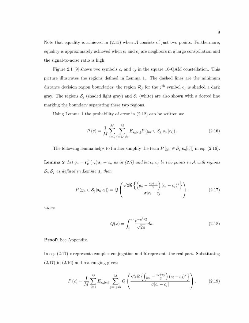
Figure 2.1 [9] shows two symbols ci and cj in the square 16-QAM constellation. This

picture illustrates the regions defined in Lemma 1. The dashed lines are the minimum

distance decision region boundaries; the region Rj for the jth symbol cj is shaded a dark

gray. The regions Sj (shaded light gray) and Si (white) are also shown with a dotted line

marking the boundary separating these two regions.

Using Lemma 1 the probability of error in (2.12) can be written as:

P (e) =1

M

M∑

i=1

M∑

j=1,j 6=i

Esn[ci]P (yn ∈ Sj |sn [ci]) . (2.16)

The following lemma helps to further simplify the term P (yn ∈ Sj |sn[ci]) in eq. (2.16).

Lemma 2 Let yn = rTp (τe) sn+un as in (2.7) and let ci, cj be two points in A with regions

Si,Sj as defined in Lemma 1, then

P (yn ∈ Sj |sn[ci]) = Q

√2<{(

yn − ci+cj2

)

(ci − cj)∗}

σ|ci − cj |

, (2.17)

where

Q(x) =

∫ ∞

x

e−u2/2

√2π

du. (2.18)

Proof: See Appendix.

In eq. (2.17) ∗ represents complex conjugation and < represents the real part. Substituting

(2.17) in (2.16) and rearranging gives:

P (e) =1

M

M∑

i=1

Esn[ci]

M∑

j=1j 6=i

Q

√2<{(

yn − ci+cj2

)

(ci − cj)∗}

σ|ci − cj |

. (2.19)

10

Fig. 2.1: 16-quadrature amplitude modulation (QAM) constellation.

Let

Pe (e) =1

M

M∑

i=1

M∑

j=1j 6=i

Q

√2<{(

yn − ci+cj2

)

(ci − cj)∗}

σ|ci − cj |

. (2.20)

The derivative of log (P (e)) with respect to τe using the principles from Brandwood [21]

will lead to the error signal of the timing error detector,

e =d log (P (e))

dτe=

1

Pe (e)· dP (e)

dτe, (2.21)

where dP (e)dτe

is given by:

dP (e)

dτe=

1

M

M∑

i=1

M∑

j=1j 6=i

exp

−1

2σ2

( √2

|ci − cj |<{(

yn − ci + cj2

)

(ci − cj)∗

}

)2

×

√2<{(

yn − ci+cj2

)

(ci − cj)∗}

σ|ci − cj |

. (2.22)

11

Here yn is the derivative of yn which is a function of τe.

Substituting (2.22) in (2.21) gives:

e =1

Pe (e)· 1

M

M∑

i=1

M∑

j=1j 6=i

exp

−1

2σ2

( √2

|ci − cj |<{(

yn − ci + cj2

)

(ci − cj)∗

}

)2

×

√2<{(

yn − ci+cj2

)

(ci − cj)∗}

σ|ci − cj |

. (2.23)

Approximating the function Q′(x) with Q(x) (2.23) becomes:

ea =1

Pe (e)· 1

M

M∑

i=1

M∑

j=1j 6=i

Q

1

2σ2

( √2

|ci − cj |<{(

yn − ci + cj2

)

(ci − cj)∗

}

)2

×

√2<{(

yn − ci+cj2

)

(ci − cj)∗}

σ|ci − cj |

. (2.24)

Equation (2.23) represents the exact timing error signal and (2.24) represents the ap-

proximate timing error. The symbols ci, cj , and yn in (2.24) are complex numbers. Let

ci = r1 + ir2, cj = t1 + it2 and yn = z1 + iz2 where r1, r2, t1, t2, z1, z2 are real numbers

and i =√−1. Substituting these in (2.23) and simplifying gives:

ea =1

Pe (e)· 1

M

M∑

i=1

M∑

j=1j 6=i

Q

1

2σ2

( √2

|ci − cj |<{(

yn − ci + cj2

)

(ci − cj)∗

}

)2

×( √

2

σ|ci − cj |(

z1 (r1− t1) + z2 (r2− t2))

)

. (2.25)

This looks like the error signal for maximum likelihood case, but scaled by nonlinear terms.

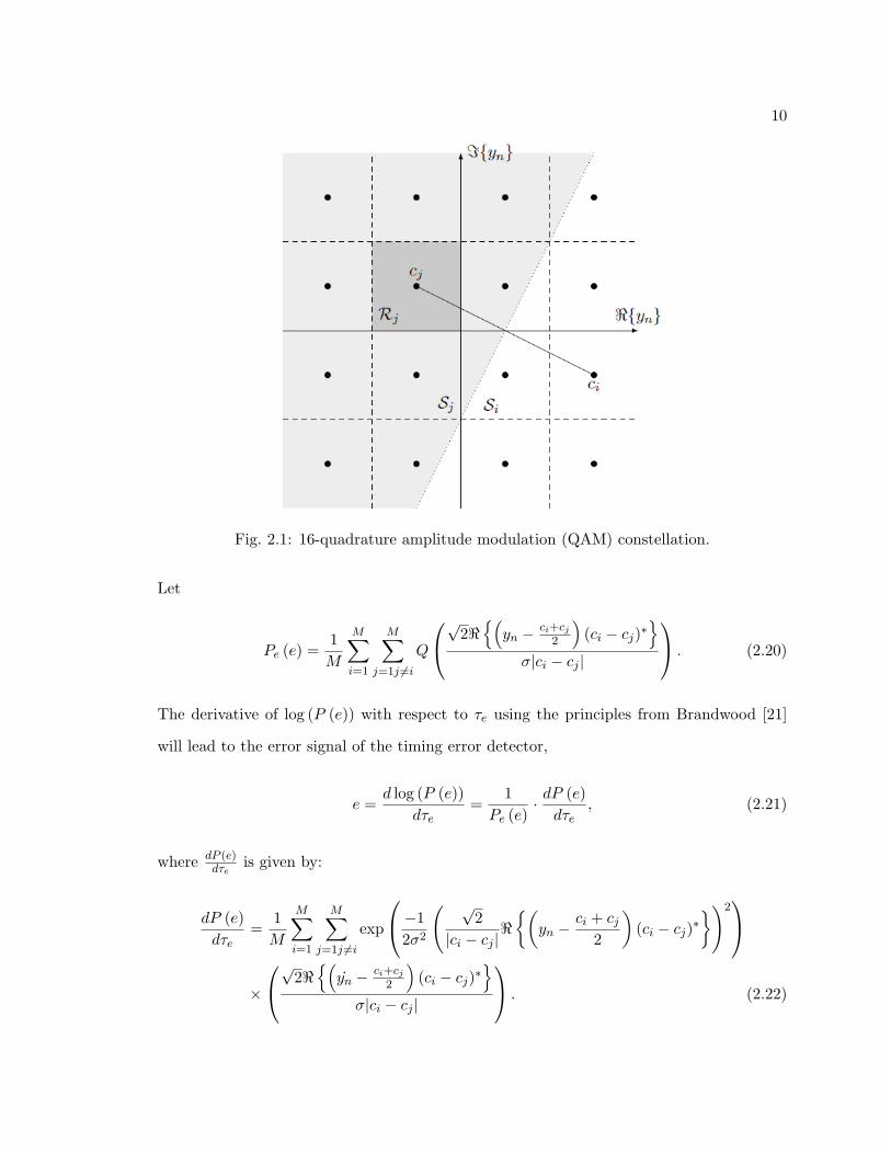
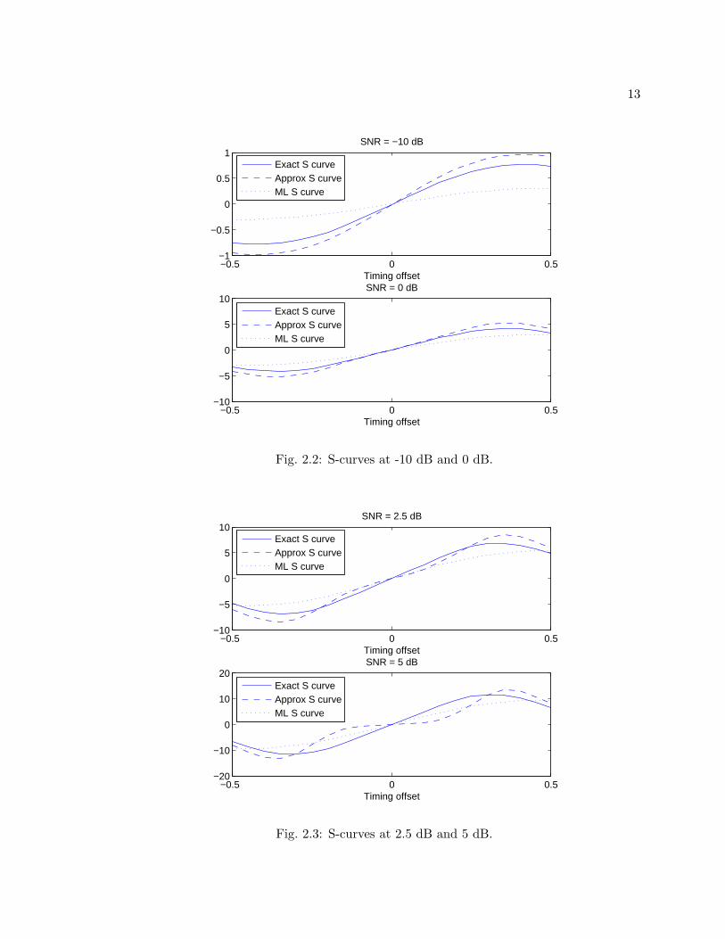
2.3 S-Curves

The S-curve is a useful tool to gain an insight on the behavior of TEDs. The term yn

is a function of τe. It can be shown that if τe = 0, then e = 0. However in order to analyze

whether the implication works in the other direction, S-curves are used. The S-curves are

obtained by plotting the error signal e or ea with respect to τe and averaging the plot over

12

the symbols. For this purpose, define:

gMSER(τe) = E {e} , (2.26)

where E represents the expectation with respect to the symbols. The function gMSER(τe)

measures the average value of error for a given timing offset τe . Using eqs. (2.23) and

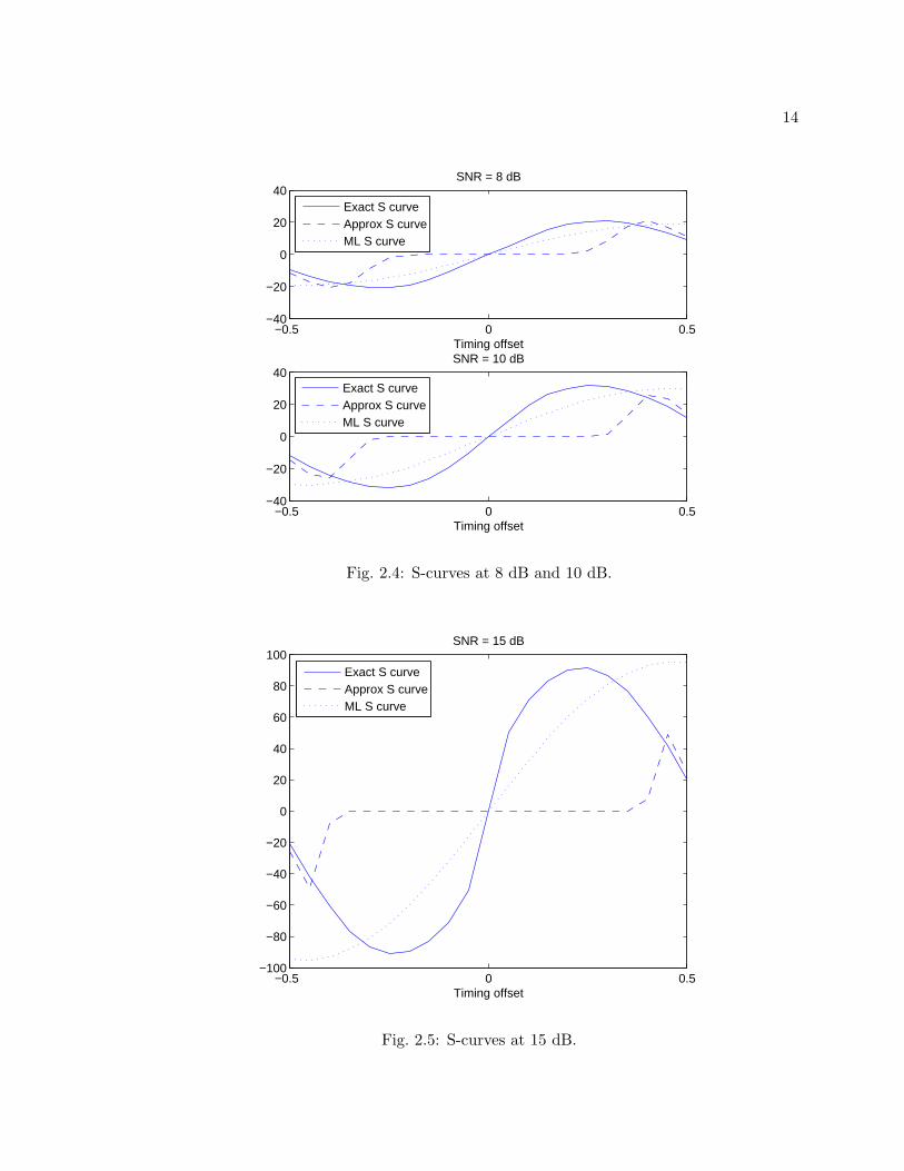
(2.24), the exact S-curves and approximate S-curves are obtained. Figures 2.2 - 2.5 show

the S-curves for different signal-to-noise ratios. The curve in solid are the exact S-curves,

the dashed ones are approximate S-curves, and for reference, MLTED S-curves are also

plotted which are the dotted ones.

The interesting point to observe from the plots is that S-curves for MSERTED have

higher slopes than MLTED S-curves. As the SNR increases, the slope of the exact S-curve

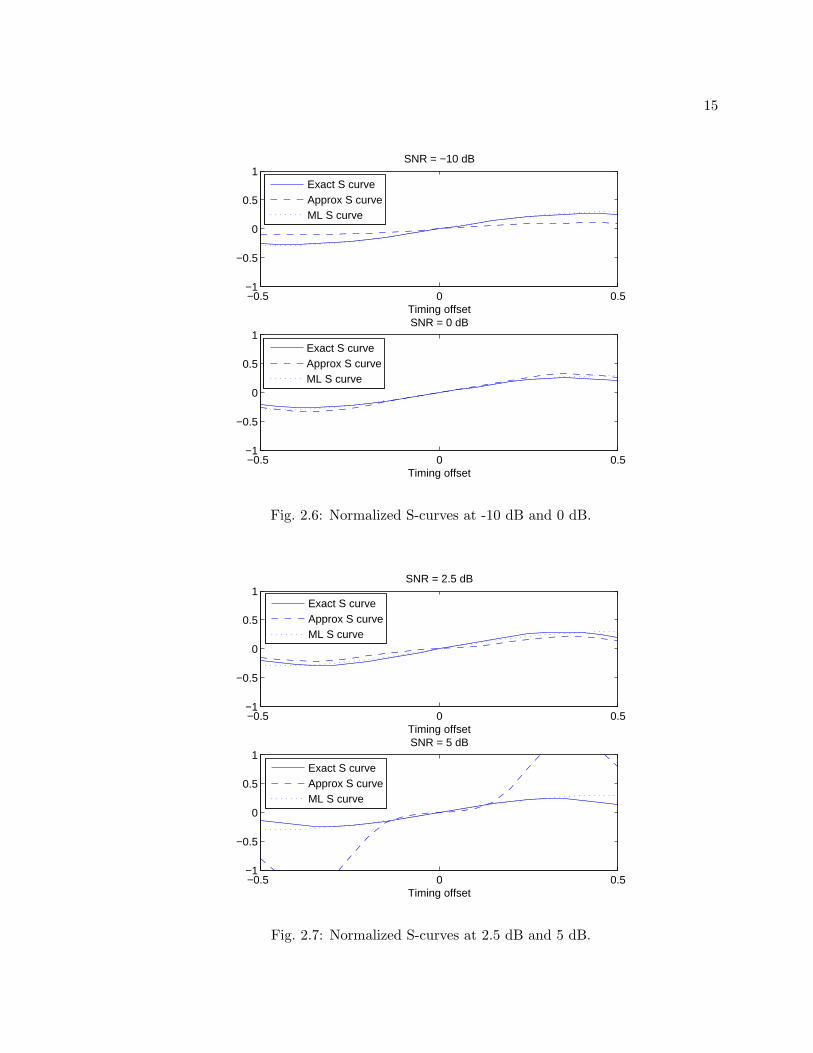
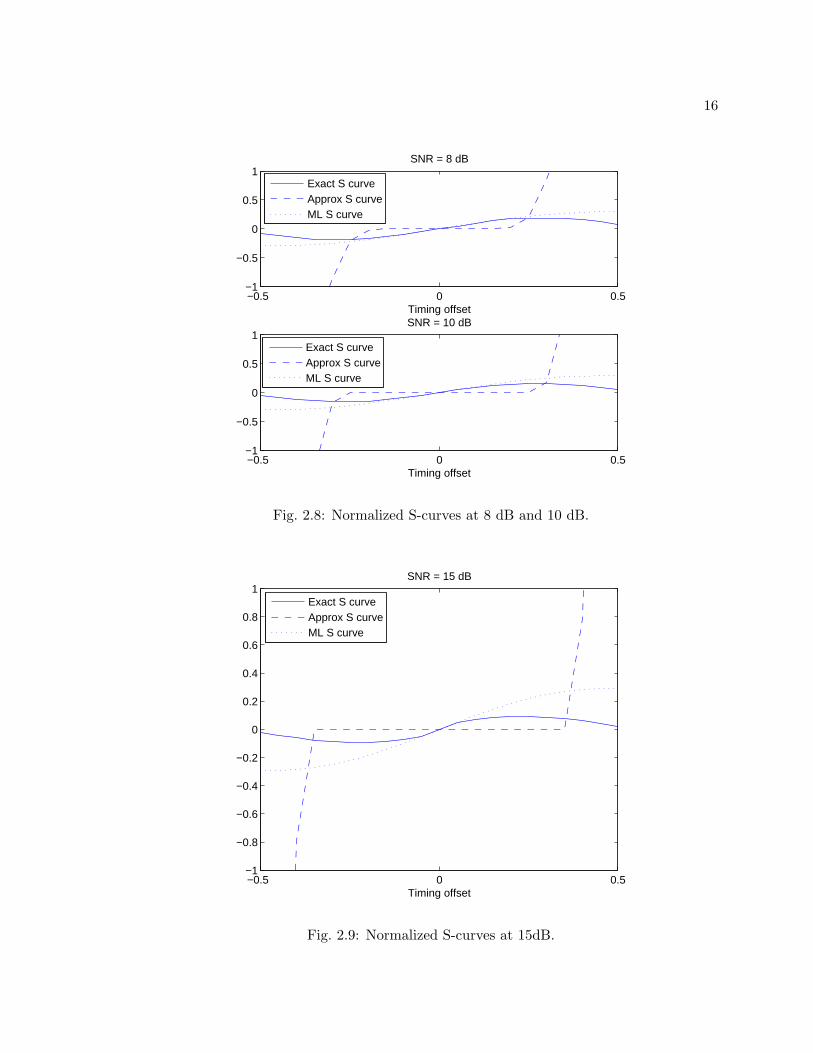
for MSERTED increases at the origin whereas the approximate one flattens. Figures 2.6

- 2.9 show the normalized S-curves. The S-curves help in calculating the TED loop param-

eters. The slope of these curves at the origin gives the “gain” denoted Kp of the TED. The

normalized S-curves provide the means for gain comparison of exact MSERTED, approxi-

mate MSERTED and the MLTED. The exact MSERTED and MLTED have pretty much

the same gains at -10 dB. For 0 dB SNR the approximate MSERTED has higher gain than

MLTED, whereas the exact MSERTED has pretty much the same behavior as MLTED. The

S-curves from 5 dB onwards looks very interesting which shows us that the approximate

MSERTED had higher gain than the ML case. At these SNRs the approximate MSERTED

will amplify the timing errors as compared to MLTED and will lead to fast convergence.

For SNRs greater than or equal to 10 dB, the step size in the adaptation process for ap-

proximate MSERTED is very high for high timing offset errors. The behavior of amplifying

the error signal produces a large timing error and makes the approximate MSERTED adapt

faster compared to MLTED. This is illustrated with the simulation results.

13

−0.5 0 0.5−1

−0.5

0

0.5

1

Timing offset

SNR = −10 dB

Exact S curveApprox S curveML S curve

−0.5 0 0.5−10

−5

0

5

10

Timing offset

SNR = 0 dB

Exact S curveApprox S curveML S curve

Fig. 2.2: S-curves at -10 dB and 0 dB.

−0.5 0 0.5−10

−5

0

5

10

Timing offset

SNR = 2.5 dB

Exact S curveApprox S curveML S curve

−0.5 0 0.5−20

−10

0

10

20

Timing offset

SNR = 5 dB

Exact S curveApprox S curveML S curve

Fig. 2.3: S-curves at 2.5 dB and 5 dB.

14

−0.5 0 0.5−40

−20

0

20

40

Timing offset

SNR = 8 dB

Exact S curveApprox S curveML S curve

−0.5 0 0.5−40

−20

0

20

40

Timing offset

SNR = 10 dB

Exact S curveApprox S curveML S curve

Fig. 2.4: S-curves at 8 dB and 10 dB.

−0.5 0 0.5−100

−80

−60

−40

−20

0

20

40

60

80

100

Timing offset

SNR = 15 dB

Exact S curveApprox S curveML S curve

Fig. 2.5: S-curves at 15 dB.

15

−0.5 0 0.5−1

−0.5

0

0.5

1

Timing offset

SNR = −10 dB

Exact S curveApprox S curveML S curve

−0.5 0 0.5−1

−0.5

0

0.5

1

Timing offset

SNR = 0 dB

Exact S curveApprox S curveML S curve

Fig. 2.6: Normalized S-curves at -10 dB and 0 dB.

−0.5 0 0.5−1

−0.5

0

0.5

1

Timing offset

SNR = 2.5 dB

Exact S curveApprox S curveML S curve

−0.5 0 0.5−1

−0.5

0

0.5

1

Timing offset

SNR = 5 dB

Exact S curveApprox S curveML S curve

Fig. 2.7: Normalized S-curves at 2.5 dB and 5 dB.

16

−0.5 0 0.5−1

−0.5

0

0.5

1

Timing offset

SNR = 8 dB

Exact S curveApprox S curveML S curve

−0.5 0 0.5−1

−0.5

0

0.5

1

Timing offset

SNR = 10 dB

Exact S curveApprox S curveML S curve

Fig. 2.8: Normalized S-curves at 8 dB and 10 dB.

−0.5 0 0.5−1

−0.8

−0.6

−0.4

−0.2

0

0.2

0.4

0.6

0.8

1

Timing offset

SNR = 15 dB

Exact S curveApprox S curveML S curve

Fig. 2.9: Normalized S-curves at 15dB.

17

Chapter 3

Implementation

3.1 Transmitter Processing

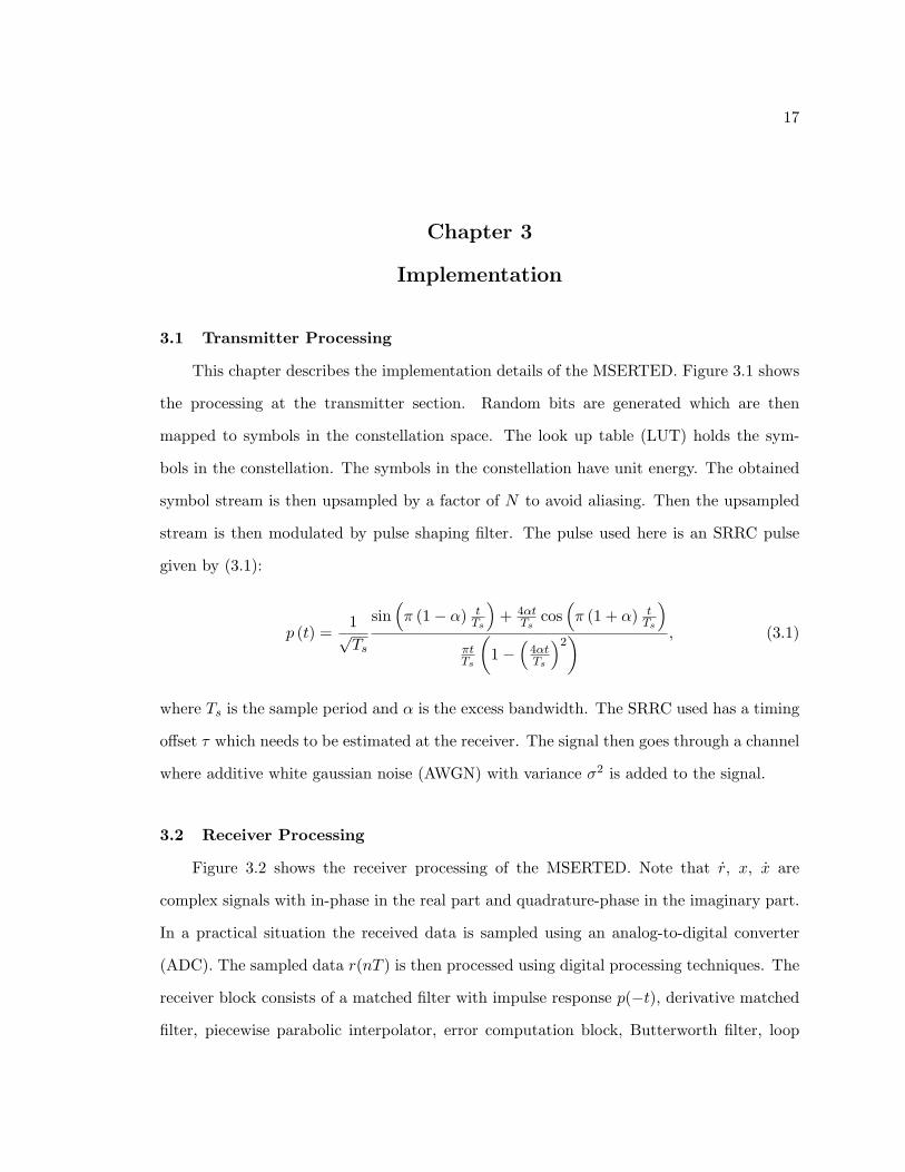
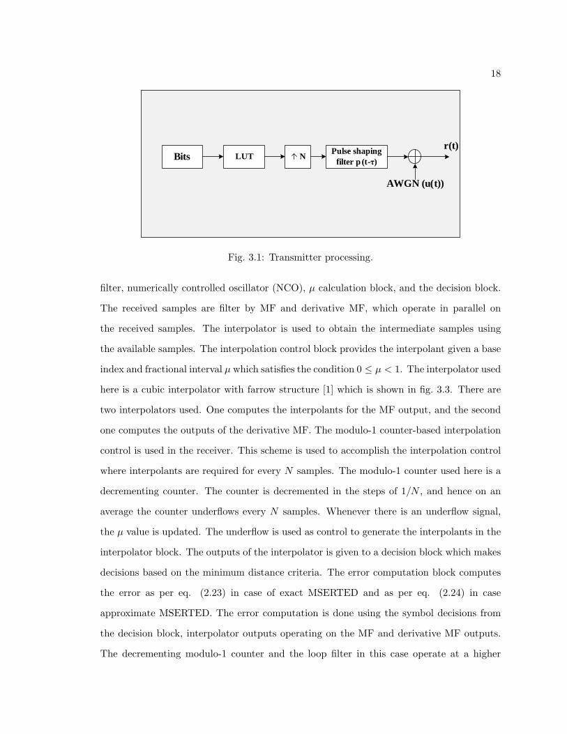
This chapter describes the implementation details of the MSERTED. Figure 3.1 shows

the processing at the transmitter section. Random bits are generated which are then

mapped to symbols in the constellation space. The look up table (LUT) holds the sym-

bols in the constellation. The symbols in the constellation have unit energy. The obtained

symbol stream is then upsampled by a factor of N to avoid aliasing. Then the upsampled

stream is then modulated by pulse shaping filter. The pulse used here is an SRRC pulse

given by (3.1):

p (t) =1√Ts

sin(

π (1− α) tTs

)

+ 4αtTs

cos(

π (1 + α) tTs

)

πtTs

(

1−(

4αtTs

)2) , (3.1)

where Ts is the sample period and α is the excess bandwidth. The SRRC used has a timing

offset τ which needs to be estimated at the receiver. The signal then goes through a channel

where additive white gaussian noise (AWGN) with variance σ2 is added to the signal.

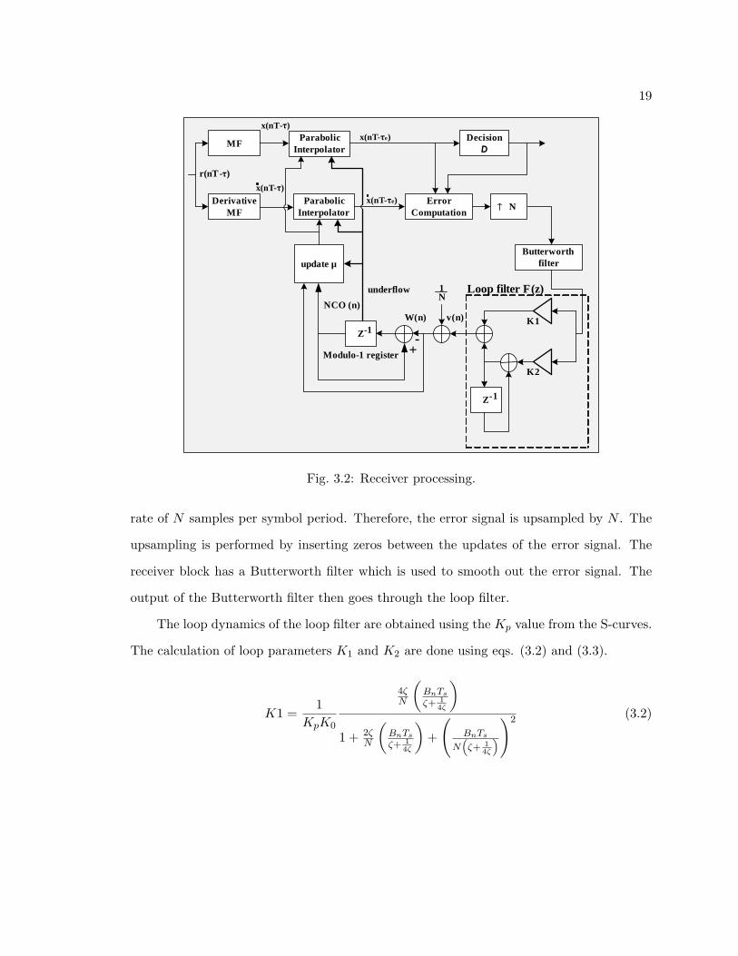
3.2 Receiver Processing

Figure 3.2 shows the receiver processing of the MSERTED. Note that r, x, x are

complex signals with in-phase in the real part and quadrature-phase in the imaginary part.

In a practical situation the received data is sampled using an analog-to-digital converter

(ADC). The sampled data r(nT ) is then processed using digital processing techniques. The

receiver block consists of a matched filter with impulse response p(−t), derivative matched

filter, piecewise parabolic interpolator, error computation block, Butterworth filter, loop

18

Bits LUT NPulse shaping

filter p (t- τ)

AWGN (u(t))

r(t)

Fig. 3.1: Transmitter processing.

filter, numerically controlled oscillator (NCO), µ calculation block, and the decision block.

The received samples are filter by MF and derivative MF, which operate in parallel on

the received samples. The interpolator is used to obtain the intermediate samples using

the available samples. The interpolation control block provides the interpolant given a base

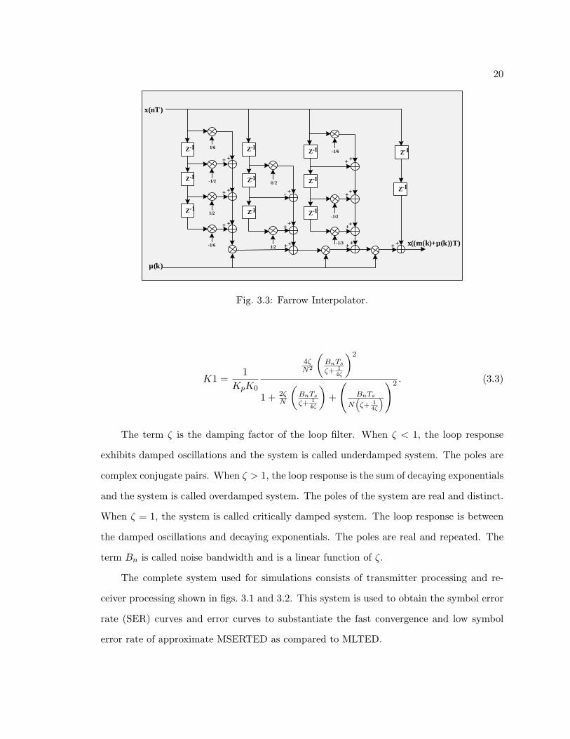
index and fractional interval µ which satisfies the condition 0 ≤ µ < 1. The interpolator used

here is a cubic interpolator with farrow structure [1] which is shown in fig. 3.3. There are

two interpolators used. One computes the interpolants for the MF output, and the second

one computes the outputs of the derivative MF. The modulo-1 counter-based interpolation

control is used in the receiver. This scheme is used to accomplish the interpolation control

where interpolants are required for every N samples. The modulo-1 counter used here is a

decrementing counter. The counter is decremented in the steps of 1/N , and hence on an

average the counter underflows every N samples. Whenever there is an underflow signal,

the µ value is updated. The underflow is used as control to generate the interpolants in the

interpolator block. The outputs of the interpolator is given to a decision block which makes

decisions based on the minimum distance criteria. The error computation block computes

the error as per eq. (2.23) in case of exact MSERTED and as per eq. (2.24) in case

approximate MSERTED. The error computation is done using the symbol decisions from

the decision block, interpolator outputs operating on the MF and derivative MF outputs.

The decrementing modulo-1 counter and the loop filter in this case operate at a higher

19

MF

r(nT-τ)

Derivative MF

Parabolic Interpolator

Parabolic Interpolator

DecisionD

Error Computation

N

Z-1

Z-1

update µ

NCO (n)

Modulo-1 register

W(n)

1N

v(n)

Butterworth filter

Loop filter F(z)underflow

x(nT-τ)

x(nT-τ)

K1

K2

+-

x(nT-τe)

x(nT-τe)

Fig. 3.2: Receiver processing.

rate of N samples per symbol period. Therefore, the error signal is upsampled by N . The

upsampling is performed by inserting zeros between the updates of the error signal. The

receiver block has a Butterworth filter which is used to smooth out the error signal. The

output of the Butterworth filter then goes through the loop filter.

The loop dynamics of the loop filter are obtained using the Kp value from the S-curves.

The calculation of loop parameters K1 and K2 are done using eqs. (3.2) and (3.3).

K1 =1

KpK0

4ζN

(

BnTs

ζ+ 1

4ζ

)

1 + 2ζN

(

BnTs

ζ+ 1

4ζ

)

+

(

BnTs

N(

ζ+ 1

4ζ

)

)2 (3.2)

20

Z-1

Z-1

Z-1

Z-1

Z-1

Z-1

Z-1

Z-1

Z-1

++

++

++

+-

+

+

1/6

-1/2

-1/6

1/2

-1/2

1/2

-1/6

-1/2

-1/3

Z-1

Z-1

+

+

++

++

++

++ ++

µ(k)

x(nT)

x((m(k)+µ(k))T)

Fig. 3.3: Farrow Interpolator.

K1 =1

KpK0

4ζN2

(

BnTs

ζ+ 1

4ζ

)2

1 + 2ζN

(

BnTs

ζ+ 1

4ζ

)

+

(

BnTs

N(

ζ+ 1

4ζ

)

)2 . (3.3)

The term ζ is the damping factor of the loop filter. When ζ < 1, the loop response

exhibits damped oscillations and the system is called underdamped system. The poles are

complex conjugate pairs. When ζ > 1, the loop response is the sum of decaying exponentials

and the system is called overdamped system. The poles of the system are real and distinct.

When ζ = 1, the system is called critically damped system. The loop response is between

the damped oscillations and decaying exponentials. The poles are real and repeated. The

term Bn is called noise bandwidth and is a linear function of ζ.

The complete system used for simulations consists of transmitter processing and re-

ceiver processing shown in figs. 3.1 and 3.2. This system is used to obtain the symbol error

rate (SER) curves and error curves to substantiate the fast convergence and low symbol

error rate of approximate MSERTED as compared to MLTED.

21

Chapter 4

Results

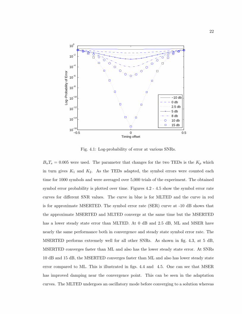
4.1 Probability of Error

This chapter discusses the results obtained by the simulation of MSERTED system.

Equation (2.19) represents the probability of error as a function of τ for the MSERTED.

Figure 4.1 shows the logarithm of probability of error as a function of τ for different SNR

values. The simulations were done for QPSK constellation with unit energy symbols. For

each value of τ the probability of error was averaged over 1000 trials of the experiment. The

pulse shape used is SRRC pulse with 50% excess bandwidth and Lp = 4. The plots show

that the probability of error is high for higher time offsets τ = 0.5Ts and τ = −0.5Ts and

decreases as the timing offset decreases. The probability of error has minimum at τ = 0.

For SNRs greater than 10dB the probability of error decreases significantly.

4.2 Symbol Error Rate

The transmitter and receiver processing blocks shown in figs. 3.1 and 3.2, respectively,

were used for the complete system simulations. The symbol error rate curves were obtained

for approximate MSERTED and the MLTED for comparing the results. The S-curves

also predicts that the exact MLTED might perform no better than MLTED. Hence, the

comparison is done between the approximate MSERTED and MLTED. The approximate

MSERTED is more practical as compared to the exact one since it has the Q function in

its arguments rather than an exponential term.

The QPSK constellation is used for the simulation of the system. The received data

was generated with timing offset τ = 0.5Ts with the noise added to it. In order to have

a fair comparison the same loop dynamics for MSERTED and MLTED were used. The

damping factor of ζ = 1/√2 and (noise equivalent bandwidth)(symbol period) product of

22

−0.5 0 0.510

−16

10−14

10−12

10−10

10−8

10−6

10−4

10−2

100

Timing offset

Log−

Pro

babi

lity

of E

rror

−10 db0 db2.5 db5 db8 db10 db15 db

Fig. 4.1: Log-probability of error at various SNRs.

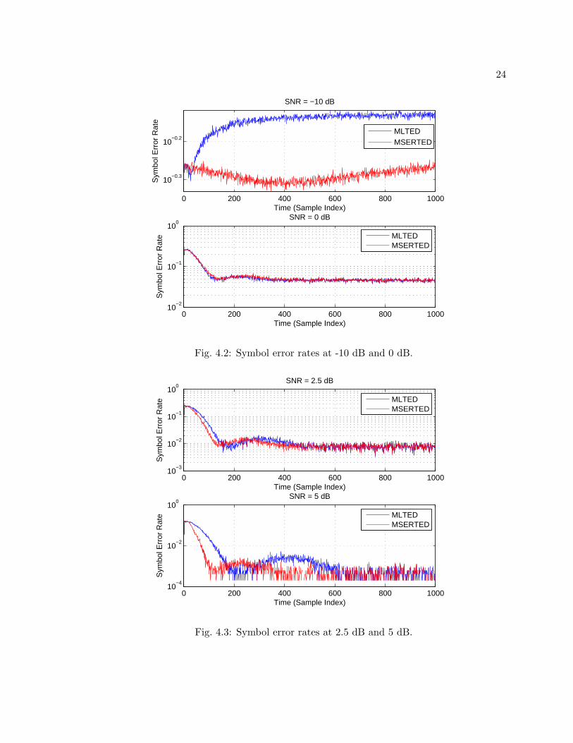
BnTs = 0.005 were used. The parameter that changes for the two TEDs is the Kp which

in turn gives K1 and K2. As the TEDs adapted, the symbol errors were counted each

time for 1000 symbols and were averaged over 5,000 trials of the experiment. The obtained

symbol error probability is plotted over time. Figures 4.2 - 4.5 show the symbol error rate

curves for different SNR values. The curve in blue is for MLTED and the curve in red

is for approximate MSERTED. The symbol error rate (SER) curve at -10 dB shows that

the approximate MSERTED and MLTED converge at the same time but the MSERTED

has a lower steady state error than MLTED. At 0 dB and 2.5 dB, ML and MSER have

nearly the same performance both in convergence and steady state symbol error rate. The

MSERTED performs extremely well for all other SNRs. As shown in fig. 4.3, at 5 dB,

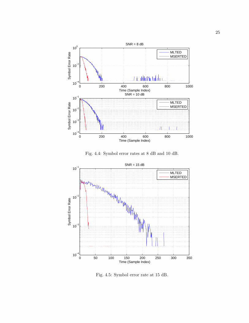
MSERTED converges faster than ML and also has the lower steady state error. At SNRs

10 dB and 15 dB, the MSERTED converges faster than ML and also has lower steady state

error compared to ML. This is illustrated in figs. 4.4 and 4.5. One can see that MSER

has improved damping near the convergence point. This can be seen in the adaptation

curves. The MLTED undergoes an oscillatory mode before converging to a solution whereas

23

MSERTED oscillations decays rapidly.

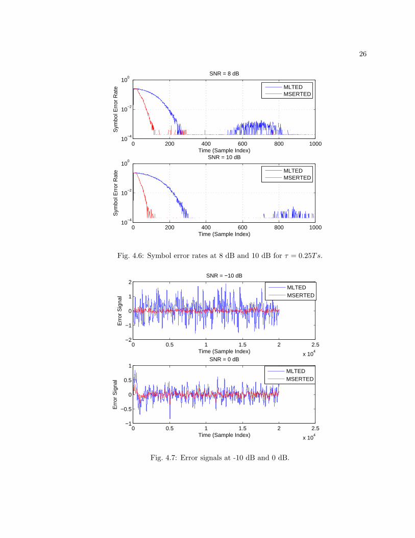
The same system was simulated with a timing offset τ = 0.25Ts for the SNRs 8 dB and

10 dB. Figure 4.6 shows the symbol error rate plots. It can be seen that the MSERTED

converges faster and have either low steady error or no errors compared to MLTED.

4.3 Error Signal Plots

The error signal is the output of the timing detector, which gives the information

about the convergence of the system towards a solution. Figures 4.7 - 4.10 show the error

signals of the approximate MSERTED and MLTED. The curve in blue is for MLTED,

and the curve in red is for approximate MSERTED. At -10 dB one can observe that both

MSER and ML converge at the same time, but the error signal amplitude is less for MSER

compared to ML, and hence low steady state error. At 0 dB and 2.5 dB, both MSER and

ML curves look similar, and from 5 dB onwards one can observe the faster convergence

and low error amplitude at the steady state. We can also observe that the MSERTED has

improved damping performance compared to MLTED. The MLTED oscillates more before

reaching the convergence point where as MSERTED has fast decaying oscillations near the

convergence point. These signals exactly correspond to the behavior exhibited by the SER

curves.

At the optimum sampling instant, the timing error is zero when there is data transition.

When there is no data transition, even at the optimum sampling instant, the timing error

may not be zero. This nonzero value is called self noise of the TED. Figure 4.11 shows a

typical plot of µ. The simulation was done for a timing offset of τ = 0.4Ts at 8 dB SNR.

We can observe that µ in case of MSERTED tries to settle faster than MLTED, but µ for

ML is more smoother than MSERTED and takes more time to settle at 0.6. This shows

that MSERTED has higher self noise than MLTED. This high self noise is due to the high

gain to the MSERTED.

24

0 200 400 600 800 1000

10−0.3

10−0.2

Time (Sample Index)

Sym

bol E

rror

Rat

e

SNR = −10 dB

MLTEDMSERTED

0 200 400 600 800 100010

−2

10−1

100

Time (Sample Index)

Sym

bol E

rror

Rat

e

SNR = 0 dB

MLTEDMSERTED

Fig. 4.2: Symbol error rates at -10 dB and 0 dB.

0 200 400 600 800 100010

−3

10−2

10−1

100

Time (Sample Index)

Sym

bol E

rror

Rat

e

SNR = 2.5 dB

MLTEDMSERTED

0 200 400 600 800 100010

−4

10−2

100

Time (Sample Index)

Sym

bol E

rror

Rat

e

SNR = 5 dB

MLTEDMSERTED

Fig. 4.3: Symbol error rates at 2.5 dB and 5 dB.

25

0 200 400 600 800 100010

−4

10−2

100

Time (Sample Index)

Sym

bol E

rror

Rat

e

SNR = 8 dB

MLTEDMSERTED

0 200 400 600 800 100010

−4

10−3

10−2

10−1

Time (Sample Index)

Sym

bol E

rror

Rat

e

SNR = 10 dB

MLTEDMSERTED

Fig. 4.4: Symbol error rates at 8 dB and 10 dB.

0 50 100 150 200 250 300 35010

−4

10−3

10−2

10−1

Time (Sample Index)

Sym

bol E

rror

Rat

e

SNR = 15 dB

MLTEDMSERTED

Fig. 4.5: Symbol error rate at 15 dB.

26

0 200 400 600 800 100010

−4

10−2

100

Time (Sample Index)

Sym

bol E

rror

Rat

e

SNR = 8 dB

MLTEDMSERTED

0 200 400 600 800 100010

−4

10−2

100

Time (Sample Index)

Sym

bol E

rror

Rat

e

SNR = 10 dB

MLTEDMSERTED

Fig. 4.6: Symbol error rates at 8 dB and 10 dB for τ = 0.25Ts.

0 0.5 1 1.5 2 2.5

x 104

−2

−1

0

1

2

Time (Sample Index)

Err

or S

igna

l

SNR = −10 dB

MLTEDMSERTED

0 0.5 1 1.5 2 2.5

x 104

−1

−0.5

0

0.5

1

Time (Sample Index)

Err

or S

igna

l

SNR = 0 dB

MLTEDMSERTED

Fig. 4.7: Error signals at -10 dB and 0 dB.

27

0 0.5 1 1.5 2 2.5

x 104

−1

−0.5

0

0.5

1

Time (Sample Index)

Err

or S

igna

l

SNR = 2.5 dB

MLTEDMSERTED

0 0.5 1 1.5 2 2.5

x 104

−1

0

1

2

Time (Sample Index)

Err

or S

igna

l

SNR = 5 dB

MLTEDMSERTED

Fig. 4.8: Error signals at 2.5 dB and 5 dB.

0 0.5 1 1.5 2 2.5

x 104

−1

0

1

2

Time (Sample Index)

Err

or S

igna

l

SNR = 8 dB

MLTEDMSERTED

0 0.5 1 1.5 2 2.5

x 104

−2

−1

0

1

2

Time (Sample Index)

Err

or S

igna

l

SNR = 10 dB

MLTEDMSERTED

Fig. 4.9: Error signals at 8 dB and 10 dB.

28

0 0.5 1 1.5 2 2.5 3 3.5 4 4.5

x 104

−1.5

−1

−0.5

0

0.5

1

1.5

2

Time (Sample Index)

Err

or S

igna

l

SNR = 15 dB

MLTEDMSERTED

Fig. 4.10: Error signal at 15 dB.

0 0.5 1 1.5 2 2.5

x 104

0

0.1

0.2

0.3

0.4

0.5

0.6

0.7

0.8

0.9

1

MLTEDMSERTED

Fig. 4.11: An example µ plot.

29

4.4 Clock Frequency Offset

This section deals with the problem of clock frequency offset. The clock frequency

offset makes the constellation continuously rotate and scatter the symbols over the entire

constellation. The new TED proposed also works better than ML in compensating the clock

frequency offset. The same system is used for the simulation with the same loop dynamics.

The error signals are plotted for frequency offsets of 0.0025 and 0.005 for SNRs 5 dB and 8

dB, respectively. The plots are shown in fig. 4.12. We can observe that MSERTED converges

faster than MLTED, and hence MSERTED has a better performance than MLTED in case

of clock frequency offset as well.

0 0.5 1 1.5 2 2.5

x 104

−2

−1

0

1

2

Time (Sample Index)

Err

or S

igna

l

SNR = 5 dB

MLTEDMSERTED

0 0.5 1 1.5 2 2.5

x 104

−2

−1

0

1

2

Time (Sample Index)

Err

or S

igna

l

SNR = 8 dB

MLTEDMSERTED

Fig. 4.12: Error signals for frequency offset of 0.0025 at 5 dB and 8 dB.

30

Chapter 5

Conclusion and Future Work

5.1 Conclusion

This thesis discusses the development and testing a new timing error detector which

minimizes the symbol error probability. The development holds good for any constellation

though the results presented are for QPSK constellation. The expressions for two timing

error detectors namely exact MSERTED and approximate MSERTED were derived. The

approximate MSERTED performs better than the traditional MLTED. The new TEDs look

like MLTED with nonlinear multiplicative terms. The other advantage of using the approx-

imate expression is the practical feasibility of the implementation. Since the expression has

a Q function it can fit into designs with a Q function look-up table. The S-curves were

used as a tool to gain an insight of the behavior of the TEDs. The sumbol error rate, the

error signal output of the TEDs, show that the approximate MSERTED converge and reach

steady state faster than MLTED. The plots also show that MSERTED have lower symbol

error rate than MLTED. Another conclusion is that we can have shorter training sequences

in case of MSERTED to achieve timing synchronization than MLTED.

5.2 Future Work

The new TED developed has a complex algorithm as compared to MLTED. In order

to achieve faster convergence and minimum symbol error rate the cost paid is the com-

plex calculations involved with the new TED. Hence in future work, it will be good if the

complexity of the algorithm is reduced so that it is quite easy to implement. However,

the approximate MSERTED can be implemented using a look up table for Q function and

interpolation techniques.

The new TED developed can be integrated with the minimum symbol error rate phase

31

recovery system developed by Gunther and Moon [5] as a future work. The new joint phase

and timing recovery system can be designed and tested against ML case for the symbol

error rate performance.

In future work, it might be a good idea to apply error correction coding techniques [22]

in conjunction with the new TED presented to achieve better performance and more reliable

communication.

32

References

[1] M. Rice, Digital Communications: A Discrete-Time Approach. Upper Saddle River,NJ: Pearson Prentice Hall, 2009.

[2] J. G. Proakis, Digital Communications. New York: McGraw-Hill, 2008.

[3] L. Franks, “Carrier and bit synchronization in data communication–A tutorial review,”IEEE Transactions on Communications, vol. 28, no. 8, pp. 1107–1121, Aug. 1980.

[4] M. Meyers and L. Franks, “Joint carrier phase and symbol timing recovery for PAMsystems,” IEEE Transactions on Communications, vol. 28, no. 8, pp. 1121–1129, Aug.1980.

[5] J. Gunther and T. Moon, “Minimum Symbol Error Rate Carrier Phase Recovery ofQPSK,” IEEE Transactions on Signal Processing, vol. 57, no. 8, pp. 3101–3107, Aug.2009.

[6] M. Aaron and D. Tufts, “Intersymbol interference and error probability,” IEEE Trans-actions on Information Theory, vol. 12, no. 1, pp. 26–34, Jan. 1966.

[7] R. Yen, “Stochastic Unbiased Minimum Mean Error Rate Algorithm for Decision Feed-back Equalizers,” IEEE Transactions on Signal Processing, vol. 55, no. 10, pp. 4758–4766, Oct. 2007.

[8] S. Chen, L. Hanzo, and B. Mulgrew, “Adaptive minimum symbol-error-rate decisionfeedback equalization for multilevel pulse-amplitude modulation,” IEEE Transactionson Signal Processing, vol. 52, no. 7, pp. 2092–2101, July 2004.

[9] J. Gunther and T. Moon, “Minimum Bayes Risk Adaptive Linear Equalizers,” IEEETransactions on Signal Processing, vol. 57, no. 12, pp. 4788–4799, Dec. 2009.

[10] C.-C. Yeh and J. Barry, “Adaptive minimum bit-error rate equalization for binarysignaling,” IEEE Transactions on Communications, vol. 48, no. 7, pp. 1226–1235, July2000.

[11] C.-C. Yeh and J. Barry, “Adaptive minimum symbol-error rate equalization forquadrature-amplitude modulation,” IEEE Transactions on Signal Processing, vol. 51,no. 12, pp. 3263–3269, Dec. 2003.

[12] C.-C. Yeh, R. Lopes, and J. Barry, “Approximate minimum bit-error rate multiuserdetection,” in Global Telecommunications Conference, 1998. The Bridge to Global In-tegration, GLOBECOM 98. IEEE, vol. 6, pp. 3590–3595, 1998.

[13] S. Chen, A. Samingan, B. Mulgrew, and L. Hanzo, “Adaptive minimum-BER linearmultiuser detection for DS-CDMA signals in multipath channels,” IEEE Transactionson Signal Processing, vol. 49, no. 6, pp. 1240–1247, June 2001.

33

[14] X. Wang, W.-S. Lu, and A. Antomiou, “Constrained minimum-BER multiuser detec-tion,” IEEE Transactions on Signal Processing, vol. 48, no. 10, pp. 2903–2909, Oct.2000.

[15] I. Psaromiligkos, S. Batalama, and D. Pados, “On adaptive minimum probability oferror linear filter receivers for DS-CDMA channels,” IEEE Transactions on Commu-nications, vol. 47, no. 7, pp. 1092–1102, July 1999.

[16] S. Chen, L. Hanzo, and N. Ahmad, “Adaptive minimum bit error rate beamformingassisted receiver for wireless communications,” in IEEE International Conference onAcoustics, Speech, and Signal Processing (ICASSP), vol. 4, pp. IV–640, 2003.

[17] T. Samir, S. Elnoubi, and A. Elnashar, “Class of minimum bit error rate algorithms,”in The 9th International Conference on Advanced Communication Technology, vol. 1,pp. 168–173, 2007.

[18] J. Bergmans and H. Wong-Lam, “A class of data-aided timing-recovery schemes,” IEEETransactions on Communications, vol. 43, no. 234, pp. 1819–1827, Feb./Mar./Apr.1995.

[19] F. Gardner, “A BPSK/QPSK timing-error detector for sampled receivers,” IEEETransactions on Communications, vol. 34, no. 5, pp. 423–429, May 1986.

[20] K. Mueller and M. Muller, “Timing recovery in digital synchronous data receivers,”IEEE Transactions on Communications, vol. 24, no. 5, pp. 516–531, May 1976.

[21] D. Brandwood, “A complex gradient operator and its application in adaptive arraytheory,” IEE Proceedings on Microwaves, Optics and Antennas, vol. 130, no. 1, pp.11–16, Feb. 1983.

[22] T. Moon, Error Correction Coding: Mathematical Methods and Algorithms. Hoboken,NJ: Wiley Interscience, 2006.

34

Appendix

35

Q-function Proof

In this appendix we examine the probability on the right hand side of (2.15) which is

the probability that the matched filter output is closer to cj than to the transmitted symbol

ci. The principles in this proof are used from the paper by Gunther and Moon [9]. First,

note that the event:

{

|yn − cj |2 < |yn − ci|2∣

∣sn[ci]}

,

is equivalent to the event:

{

0 < <{(

yn − cj + ci2

)

(cj − ci)∗

}

∣

∣sn[ci]

}

. (7.1)

Next, substitute the model (2.7) into (7.1) to obtain:

{

0 < <{(

un + rTp (τe) sn − cj + ci2

)

(cj − ci)∗

}

∣

∣sn[ci]

}

. (7.2)

The rearranging of (7.2) yields:

{

<{−u(ci − cj)∗} > <

{(

rTp (τe) sn − ci + cj2

)

(ci − cj)∗

}

∣

∣sn[ci]

}

. (7.3)

Note that −u can be replaced by u because they have the same distribution. Now, if u

is zero mean and Gaussian with variance σ2, then v = u(ci− cj)∗ is Gaussian with variance

of |ci − cj |2σ2 and the real part of v = vr + jvi has variance σr2 = |ci − cj |2σ2/2. The

probability of the even in (7.3) is computed as follows:

P (vr > z|sn[ci]) =∫ ∞

z

e−v2r/2σ2r

√

2πσ2r

, ν = vr/σr

=

∫ ∞

z/σ2r

e−ν2/2

√2π

dν

= Q(z/σr). (7.4)

36

Substituting the definitions of z and σr yields:

Q

√2<{(

rTp (τe) sn − ci+cj2

)

(ci − cj)∗}

σ|ci − cj |

. (7.5)

Substituting the model from (2.7) into (7.5) gives:

Q

√2<{(

yn − ci+cj2

)

(ci − cj)∗}

σ|ci − cj |

. (7.6)