Minimum-Time Trajectory Optimization of Multiple

Revolution Low-Thrust Earth-Orbit Transfers

Kathryn F. Graham∗

Anil V. Rao†

University of FloridaGainesville, FL 32611-6250

Abstract

The problem of determining high-accuracy minimum-time Earth-orbit transfers using low-thrustpropulsion is considered. The optimal orbital transfer problem is posed as a constrained nonlinear opti-mal control problem and is solved using a variable-order Legendre-Gauss-Radau quadrature orthogonalcollocation method. Initial guesses for the optimal control problem are obtained by solving a sequenceof modified optimal control problems where the final true longitude is constrained and the mean squaredifference between the specified terminal boundary conditions and the computed terminal conditions isminimized. It is found that solutions to the minimum-time low-thrust optimal control problem are onlylocally optimal in that the solution has essentially the same number of orbital revolutions as that ofthe initial guess. A search method is then devised that enables computation of solutions with an evenlower cost where the final true longitude is constrained to be different from that obtained in the originallocally optimal solution. A numerical optimization study is then performed to determine optimal trajec-tories and control inputs for a range of initial thrust accelerations and constant specific impulses. Thekey features of the solutions are then determined, and relationships are obtained between the optimaltransfer time and the optimal final true longitude as a function of the initial thrust acceleration andspecific impulse. Finally, a detailed post-optimality analysis is performed to verify the close proximityof the numerical solutions to the true optimal solution.

Nomenclature

a = Semi-major Axis, me = Eccentricityf = Second Modified Equinoctial Elementg = Third Modified Equinoctial Elementge = Sea Level Acceleration Due to Earth Gravity, m/s2

H = Optimal Control Augmented Hamiltonianh = Second Modified Equinoctial Elementi = Inclination, deg or rad(ir, iθ, ih) = Rotating Radial Coordinate SystemJ2 = Second Zonal HarmonicJ3 = Third Zonal HarmonicJ4 = Fourth Zonal Harmonick = Fifth Modified Equinoctial Element

∗Ph.D. Student, Department of Mechanical and Aerospace Engineering. E-mail: kschuber@ufl.edu.†Associate Professor, Department of Mechanical and Aerospace Engineering. E-mail: anilvrao@ufl.edu. Associate Fellow,

AIAA. Corresponding Author.

1

L = Sixth Modified Equinoctial Element (True Longitude), rad or degm = Mass, kgn = Mean MotionPk = Legendre Polynomial of Degree kp = First Modified Equinoctial Element (Semi-Parameter), mRe = Radius of the Earth, mT = Thrust, Nt = Time, s or du = Control Directionur = Radial Component of Controluθ = Tangential Component of Controluh = Normal Component of Control∆ = Spacecraft Specific Force, m·s−2

λ = Optimal Control Costateµ = Optimal Control Path Constraint Lagrange Multiplierµe = Earth Gravitational Parameter, m3·s−2

ν = True Anomaly, deg or radΩ = Longitude of Ascending Node, deg or radω = Argument of Periapsis, deg or rad

1 Introduction

Low-thrust propulsion systems are typically characterized by high specific impulses and small initial thrustaccelerations (thrust-to-initial-mass) on the order of O(10−4) m·s−2. The use of low-thrust propulsionhas been studied extensively for orbital rendezvous, orbit maintenance, orbit transfer, and interplanetaryspace mission applications. While the efficiency of low-thrust propulsion is highly appealing, the resultingtrajectory design problem is particularly challenging to solve. For example, the high specific impulse ofa low-thrust engine combined with the small engine specific force leads to computational challenges dueto the long duration of the orbital transfer. In addition, the trajectory design problem is particularlyproblematic when the initial and terminal orbits are widely spaced resulting in a trajectory that requires alarge number of orbital revolutions in order to complete the transfer. Then, even if a solution is obtained,it is highly likely that the trajectory is not the global optimal solution.1

Low-thrust trajectory optimization has been the subject of much previous research. In Refs. 1–8numerical optimization techniques were used for to optimize interplanetary space trajectories. In Ref. 9 avariation of parameters approach was employed to solve a minimum-fuel time-fixed rendezvous problem,while in Ref. 10 Pontryagin’s minimum principle11,12 was used to determine the optimal thrust accelerationfor an orbit maintenance study. In Ref. 13 optimal control theory was used to solve minimum-time, circle-to-circle, constant thrust orbit raising and simple graphical and analytical tools were used that relatedvehicle design parameters to orbit design parameters. In addition, a variety of approximation methodshave been developed to overcome the computational challenge associated with the large number of orbitalrevolutions typical of a low-thrust orbital transfer. One of the most common approximation techniques isorbital averaging where simple approximations are derived to express incremental changes in the orbitalelements for each orbital revolution. Using orbital averaging, in Ref. 14 the problem of minimum-fuel power-limited transfers between coplanar elliptic orbits was studied, while in Ref. 15 near-optimal, minimum-timelow-Earth orbit (LEO) to geostationary orbit (GEO) and geosynchronous transfer orbit (GTO) to GEOtransfers were examined. In addition, in Ref. 16 a parameterized control law was employed togetherwith orbital averaging in order to solve three common near-optimal, minimum-time Earth-orbit transfers.More recently, in Ref. 5 an orbital averaging approach was developed in conjunction with hybrid controlformulations to solve LEO to GEO and GTO to GEO transfers. Next, in Ref. 17 a 100-revolution LEOto GEO coplanar transfer was solved using direct collocation paired with a Runge-Kutta parallel-shooting

2

scheme, while in Ref. 18 a single shooting method was combined with a homotopic approach to solve aminimum-fuel transfer from a low, elliptic, and inclined orbit to GEO. In order to increase accuracy overorbital averaging techniques, in Ref. 19 sequential quadratic programming (SQP) was used with directcollocation to solve a minimum-fuel low-thrust near-polar Earth-orbit transfer with over 578 revolutions.In Ref. 20 an anti-aliasing method utilizing direction collocation was developed to obtain solutions to simplelow-thrust trajectory optimization problems. Finally, in Ref. 21 a minimum-time LEO to high-Earth orbit(HEO) transfers was solved using direct collocation with a single specific impulse value.

While a great deal of progress has been made in low-thrust trajectory optimization, much of this workfocuses on determining near-optimal solutions and very little work has been done to verify the optimalityof the solutions obtained. The contribution of this research is on determining high-accuracy solutions tominimum-time low-thrust trajectory optimization problems for a wide-range of initial thrust accelerationsand specific impulse values. Specifically, in this paper a variable-order Gaussian quadrature orthogonalcollocation method22–29 is used to determine minimum-time optimal trajectories of two common low-thrustEarth-orbit transfers. As a result, solutions to the optimal control problem are obtained without having toreplace the equations of motion with averaged approximations over each orbital revolution such as in usingan orbital averaging technique. Using the aforementioned collocation method, an initial guess generationmethod is used together with a simple search method to determine the solution that has the lowest costamongst a range of locally optimal solutions. Numerical solutions are generated for a range of initial thrustacceleration values and specific impulse values that are typical of a low-thrust propulsion system. Then, ina manner similar to that of Ref. 21, regression analyses are performed to determine the transfer time as afunction of the initial thrust acceleration and the specific impulse and to determine the final true longitudeas a function of the transfer time. From these regressions it is possible to estimate the transfer time andfinal true longitude for different initial thrust accelerations and specific impulses without having to re-solvethe optimal control problem. A post-optimality analysis is then performed to verify the optimality of thesolutions obtained in this study.

This paper is organized as follows. Section 2 describes the minimum-time low-thrust orbit transfertrajectory optimization problem solved in this research. Section 3 describes the direct collocation methodused to solve the optimal orbital transfer problem. Section 4 describes the numerical results obtainedin this study and includes a post-optimality analysis to verify the optimality of the solutions obtained.Finally, Section 5 provides conclusions on this work.

2 Low-Thrust Earth-Orbit Transfer Optimal Control Problem

Consider the problem of transferring a spacecraft from an initial Earth-orbit to a final Earth-orbit usinglow-thrust propulsion. The objective is to determine the minimum-time trajectory and control that transferthe spacecraft from the specified initial orbit to the specified terminal orbit. The low-thrust optimal controlproblem for the orbit transfer is now described.

2.1 Equations of Motion

The dynamics of the spacecraft, modeled as a point mass, are described using modified equinoctial elementstogether with a fourth-order oblate gravity model and a continuous thrust propulsion system. The state ofthe spacecraft is comprised of the modified equinoctial elements (p, f, g, h, k, L)30 together with the mass,m, where p is the semi-parameter, f and g are modified equinoctial elements that describe the eccentricityof the orbit, h and k are modified equinoctial elements that describe the inclination of the orbit, andL is the true longitude. The control is the thrust direction, u, where u is expressed in rotating radial

3

coordinates as u = (ur, uθ, uh). The differential equations of motion of the spacecraft are given as

dp

dt=

√p

µe

2p

q∆θ ≡ Fp,

df

dt=

√p

µe

(sinL ∆r + 1

q

((q + 1) cosL+ f

)∆θ − g

q

(h sinL− k cosL

)∆h

)≡ Ff ,

dg

dt=

√p

µe

(− cosL ∆r + 1

q

((q + 1) sinL+ g

)∆θ + f

q

(h sinL− k cosL

)∆h

)≡ Fg,

dh

dt=

√p

µe

s2 cosL

2q∆h ≡ Fh,

dk

dt=

√p

µe

s2 sinL

2q∆h ≡ Fk,

dL

dt=

√p

µe

(h sinL− k cosL

)∆h +

õep

(q

p

)2

≡ FL,

dm

dt= − T

geIsp≡ Fm,

(1)

whereq = 1 + f cosL+ g sinL, r = p/q,

α2 = h2 − k2, s2 = 1 +√h2 + k2.

(2)

In this research, time is replaced as the independent variable in favor of the true longitude, L, because Lprovides a more intuitive understanding of the transfer. Since the spacecraft moves from an orbit close tothe Earth to GEO, more true longitude cycles will be completed in a given amount of time near the startof the transfer than will be completed near the terminus of the transfer. Using the true longitude as theindependent variable, the differential equation for L is replaced with the differential equation

dt

dL=

1

FL= F−1

L ≡ Gt, (3)

while the remaining six differential equations for (p, f, g, h, k,m) that describe the dynamics of the space-craft are given as

dp

dL= F−1

L Fp ≡ Gp,df

dL= F−1

L Ff ≡ Gh,dg

dL= F−1

L Fg ≡ Gg,dh

dL= F−1

L Fh ≡ Gh,dk

dL= F−1

L Fk ≡ Gk,dm

dL= F−1

L Fm ≡ Gm.

(4)

Next, the spacecraft acceleration, ∆ = (∆r,∆θ,∆h), is modeled as

∆ = ∆g + ∆T , (5)

where ∆g is the gravitational acceleration due to the oblateness of the Earth and ∆T is the thrust specificforce. The acceleration due to Earth oblateness is expressed in rotating radial coordinates as

∆g = QTr δg, (6)

4

where Qr =[ir iθ ih

]is the transformation from rotating radial coordinates to Earth-centered inertial

coordinates and whose columns are defined as

ir =r

‖r‖ , ih =r× v

||r× v|| , iθ = ih × ir. (7)

Furthermore, the vector δg is defined as

δg = δgnin − δgrir (8)

where in is the local North direction and is defined as

in =en − (eTn ir)ir||en − (eTn ir)ir||

(9)

and en = (0, 0, 1). The oblate earth perturbations are then expressed as

δgr = −µer2

4∑k=2

(k + 1)

(Rer

)kPk(sinφ)Jk, (10)

δgn = −µe cosφ

r2

4∑k=2

(Rer

)kP′k(sinφ)Jk, (11)

where Re is the equatorial radius of the earth, Pk is the kth-degree Legendre polynomial, P′k is the derivative

of Pk with respect to sinφ, and Jk represents the zonal harmonic coefficients for k = (2, 3, 4). Next, thethrust specific force is given as

∆T =T

mu. (12)

Finally, the physical constants used in this study are given in Table 2.

Table 2: Physical Constants.

Quantity Value

ge 9.80665 m · s−2

µe 3.9860047× 1014 m3 · s−2

Re 6378140 m

J2 1082.639× 10−6

J3 −2.565× 10−6

J4 −1.608× 10−6

2.2 Boundary Conditions and Path Constraints

The boundary conditions for the orbit transfer are described in terms of both classical orbital elementsand modified equinoctial elements. The spacecraft starts in either a near circular inclined low-Earth orbit(LEO) or a geostationary transfer orbit (GTO) at time t0 = 0. The initial orbit is specified in terms ofclassical orbital elements31 as

a(L0) = a0, Ω(L0) = Ω0,

e(L0) = e0, ω(L0) = ω0,

i(L0) = i0, ν(L0) = ν0,

(13)

where a is the semi-major axis, e is the eccentricity, i is the inclination, Ω is the longitude of the ascendingnode, ω is the argument of periapsis, and ν is the true anomaly. Equation (13) can be expressed equivalently

5

in terms of the modified equinoctial elements as

p(L0) = a0(1− e20), h(L0) = tan(i0/2) sin Ω0,

f(L0) = e0 cos(ω0 + Ω0), k(L0) = tan(i0/2) cos Ω0,

g(L0) = e0 sin(ω0 + Ω0), L0 = Ω0 + ω0 + ν0.

(14)

For both cases considered, the spacecraft terminates in a geostationary orbit (GEO). The GEO terminalorbit is specified in classical orbital elements as

a(Lf ) = af , Ω(Lf ) = Free,

e(Lf ) = ef , ω(Lf ) = Free,

i(Lf ) = if , ν(Lf ) = Free.

(15)

Equation (15) can be expressed equivalently in terms of the modified equinoctial elements as

p(Lf ) = af (1− e2f ),(

f2(Lf ) + g2(Lf )

)1/2

= ef ,(h2(Lf ) + k2(Lf )

)1/2

= tan(if/2).

(16)

Finally, during the transfer the thrust direction must be a vector of unit length. Thus, equality pathconstraint

‖u‖2 = u2r + u2

θ + u2h = 1 (17)

is enforced throughout the orbital transfer.

2.3 Optimal Control Problem

The goal of this study is to determine solutions to the following constrained nonlinear optimal control prob-lem. Determine the trajectory (p(L), f(L), g(L), h(L), k(L),m(L), t(L)) and the control (ur(L), uθ(L), uh(L))that minimize the cost functional

J = αtf , (18)

subject to the dynamic constraints of Eqs. (3) and (4), the initial conditions of Eq. (14), the terminalconditions of Eq. (16), and the path constraints of Eq. (17). Finally, it is noted that α = 1/86400 is theconversion factor from units of seconds to units of days.

3 Numerical Solution of Low-Thrust Optimal Control Problem

The minimum-time low-thrust optimal control problem described in this paper was solved using the optimalcontrol software GPOPS− II.29 GPOPS− II is a MATLAB software that transcribes the optimal controlproblem to a nonlinear programming problem (NLP) that implements the variable-order Legendre-Gauss-Radau quadrature collocation method described in Refs. 26,27, and 32 together with an hp adaptive meshrefinement method (see Refs. 28, 33, and 34). In this study the NLP arising from the LGR collocationmethod is solved using the open-source NLP solver IPOPT 35 with analytical first and second derivativesobtained using the open-source algorithmic differentiation package ADiGator whose method is described inRef. 36. The remainder of this section is organized as follows. First, an approach is described for generatinginitial guesses for solving the optimal control problem. Second, because the solutions obtained from theNLP are only locally optimal, a motivation is provided for developing a simple search method to obtainsolutions that are closer to the global optimal. Finally, the developed simple search method is describedand is applied to the low-thrust trajectory optimization problem.

6

3.1 Initial Guess Generation

In order to solve the low-thrust orbital transfer optimal control problem described in Section 2, it wasnecessary to provide initial guesses from which the NLP solver would converge to a solution. Because thisresearch is focused on solving a problem whose solution will result in a large number of orbital revolutions,the initial guess must itself contain a number of orbital revolutions that is reasonably close to the actualnumber of orbital revolutions of the solution obtained by the NLP solver. In this paper, an initial guessprocedure was devised where a sequence of optimal control sub-problems were solved. The goal of eachsub-problem was to determine the state and control that transfer the spacecraft from the initial orbit tothe terminal conditions that minimize the following mean square relative difference:

J =

[p(Lf )− pd

1 + pd

]2

+

[f2(Lf ) + g2(Lf )− e2

d

1 + e2d

]2

+

[h2(Lf ) + k2(Lf )− tan2( id2 )

1 + tan2( id2 )

]2

. (19)

In other words, the objective of the optimal control sub-problem is to attain a solution that is as close inproximity to the desired terminal semi-parameter, pd, eccentricity, ed, and inclination, id. Each sub-problemis evaluated at most over one true longitude cycle using the terminal state of the previous sub-problemas the initial state of the current sub-problem. The continuous-time optimal control sub-problem is thenstated as follows. Minimize the cost functional of Eq. (19) subject to the dynamic constraints of Eqs. (3)and (4), the path constraint of Eq. (17), and the boundary conditions

p(r)(L(r)0 ) = p(r−1)(L

(r−1)f ), p(r)(L

(r)f ) = Free,

f (r)(L(r)0 ) = f (r−1)(L

(r−1)f ), f (r)(L

(r)f ) = Free,

g(r)(L(r)0 ) = g(r−1)(L

(r−1)f ), g(r)(L

(r)f ) = Free,

h(r)(L(r)0 ) = h(r−1)(L

(r−1)f ), h(r)(L

(r)f ) = Free,

k(r)(L(r)0 ) = k(r−1)(L

(r−1)f ), k(r)(L

(r)f ) = Free,

m(r)(L(r)0 ) = m(r−1)(L

(r−1)f ), m(r)(L

(r)f ) = Free,

L(r)0 = L

(r−1)f , L

(r)f ≤ L

(r−1)f + 2π,

(20)

for r = 1, . . . , R where R represents the total number of true longitude cycles. The initial conditions forthe first cycle, when r = 1, are simply the initial conditions stated in Eq. (14). Once the desired terminalconditions, as stated in Eq. (16), are obtained within a user specified tolerance, the sub-problem solutionsare then combined to form the initial guess. The initial mesh is comprised of intervals based on the totalnumber of true longitude cycles and an arbitrarily chosen number of collocation points assigned to eachinterval.

3.2 Search Method to Assist in Obtaining Globally Optimal Solution

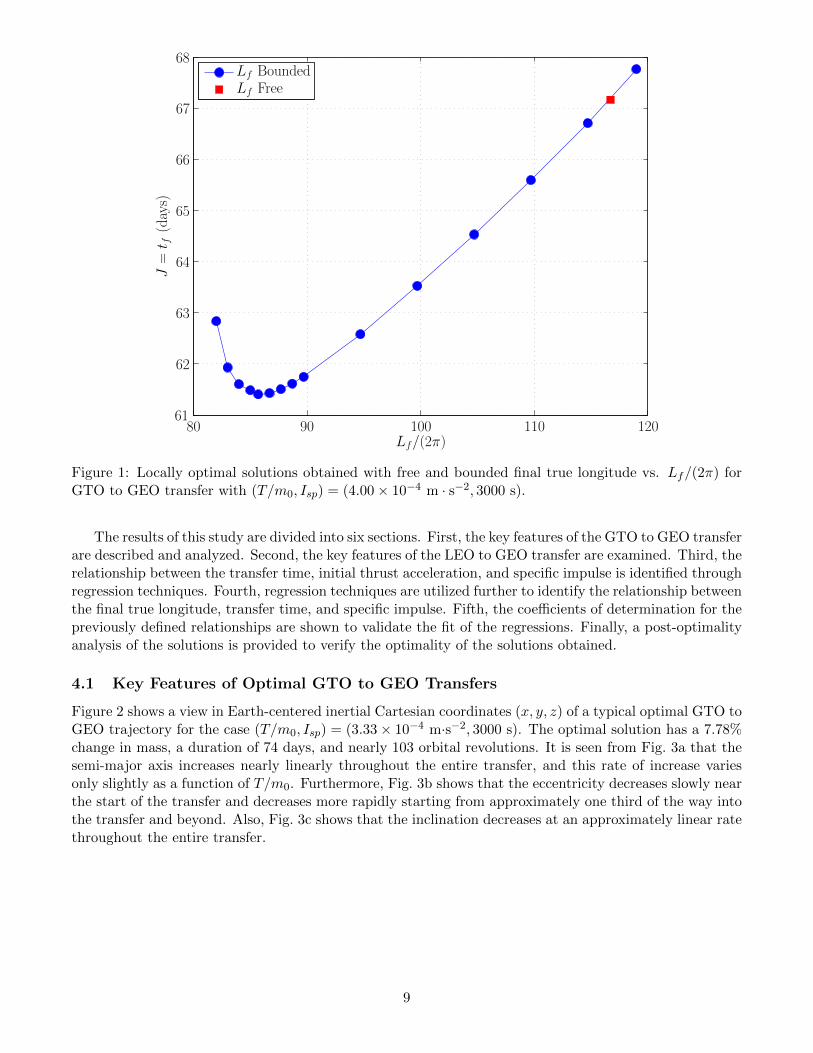
It is generally the case that gradient-based optimization methods converge to locally optimal solutions asopposed to globally optimal solutions. In the case of the low-thrust orbital transfer problems solved in thisresearch, it was found that the optimal solution typically contained the same number of true longitudecycles as that of the initial guess due to the fact that the initial guess was very close to satisfying theterminal constraints. Thus, while the NLP solver converges with the initial guess provided, the solutionis usually not the global optimal. In order to obtain a solution with a number of true longitude cyclesdifferent from that of the initial guess, the final true longitude was bounded within a specified cycle (thatis, to lie within a specified interval of 2π). By bounding the final true longitude, the NLP solver is forcedto deviate from the initial guess and potentially move closer to a global solution. Figure 1 shows the costobtained when the final true longitude is bounded as described above and when the final true longitude isfree for the GTO to GEO orbit transfer with (T/m0, Isp) = (4.00 × 10−4 m · s−2, 3000 s). It is seen from

7

Fig. 1 that the solution obtained using the provided initial guess with a free terminal true longitude doesnot have the lowest cost solution. Instead, the lowest cost lies somewhere between 80 and 90 true longitudecycles.

Based on the structure shown in Fig. 1, the following simple search method is used to identify theapproximate location of the globally optimal solution. First, an initial guess is generated as described in

Section 3.1 and the final true longitude that is obtained from this initial guess, denoted L(0)f , is the starting

point for the search method. An iteration on the final true longitude is then performed as follows, where

K is the iteration number and K = 0 corresponds to L(0)f . The optimal control problem is solved for a

final true longitude Lf ∈ [L(K)f − 2π, L

(K)f ] = I(K)

l and the cost obtained from this solution is denoted

J(K)l . Next, in order to determine which direction to search for a lower cost solution, the optimal control

problem is solved again for a final true longitude Lf ∈ [L(K)f , L

(K)f + 2π] = I(K)

r and the cost associated

with this solution is denoted J(K)r . The cycle that contains the lowest cost is then obtained using the

following iterative process:

• Set K → K + 1.

• Case 1 (minimum lies to the right of the initialization): If J(K−1)l > J

(K−1)r , then set L

(K)f =

L(K−1)f + 2π, I(K)

l = I(K−1)r , J

(K)l = J

(K−1)r , and I(K)

r = [L(K)f , L

(K)f + 2π]. Then solve the optimal

control problem again for Lf ∈ I(K)r and the cost obtained is denoted J

(K)r . Repeat until J

(K)l < J

(K)r .

The lowest cost is J(K)l with Lf ∈ I(K)

l .

• Case 2 (minimum lies to the left of the initialization): If J(K−1)l < J

(K−1)r , then set L

(K)f = L

(K−1)f −

2π, I(K)r = I(K−1)

l , J(K)r = J

(K−1)l , and I(K)

l = [L(K)f − 2π, L

(K)f ]. Then solve the optimal control

problem again for Lf ∈ I(K)l and the cost obtained is denoted J

(K)l . Repeat until J

(K)r < J

(K)l . The

lowest cost is J(K)r with Lf ∈ I(K)

r .

4 Results and Discussion

The GTO to GEO Earth-orbit transfer problem was solved using the following initial orbit:

a(L0) = 24443 km, Ω(L0) = 0 deg,

e(L0) = 0.725, ω(L0) = 0 deg,

i(L0) = 7 deg, ν(L0) = 0 deg,

(21)

while the LEO to GEO Earth-orbit transfer problem was solved using the following initial orbit:

a(L0) = 6656 km, Ω(L0) = 0 deg,

e(L0) = 0.001, ω(L0) = 0 deg,

i(L0) = 28.5 deg, ν(L0) = 0 deg.

(22)

Both the GTO to GEO and LEO to GEO Earth-orbit transfer problems were solved using the followingterminal orbit:

a(Lf ) = 42164 km, Ω(Lf ) = Free,

e(Lf ) = 0, ω(Lf ), = Free,

i(Lf ) = 0 deg, ν(Lf ) = Free.

(23)

The minimum-time GTO to GEO and LEO to GEO transfers were solved with initial thrust accelerationvalues of T/m0 = (2.000, 1.000, 0.667, 0.500, 0.400, 0.333, 0.286, 0.250, 0.222, 0.200)×10−3 m·s−2 and specificimpulse values of Isp = (500, 1000, 3000, 5000) s.

8

Lf/(2π)

J=t f

(days)

68

67

66

65

64

63

62

6180 90 100 110 120

Lf BoundedLf Free

Figure 1: Locally optimal solutions obtained with free and bounded final true longitude vs. Lf/(2π) forGTO to GEO transfer with (T/m0, Isp) = (4.00× 10−4 m · s−2, 3000 s).

The results of this study are divided into six sections. First, the key features of the GTO to GEO transferare described and analyzed. Second, the key features of the LEO to GEO transfer are examined. Third, therelationship between the transfer time, initial thrust acceleration, and specific impulse is identified throughregression techniques. Fourth, regression techniques are utilized further to identify the relationship betweenthe final true longitude, transfer time, and specific impulse. Fifth, the coefficients of determination for thepreviously defined relationships are shown to validate the fit of the regressions. Finally, a post-optimalityanalysis of the solutions is provided to verify the optimality of the solutions obtained.

4.1 Key Features of Optimal GTO to GEO Transfers

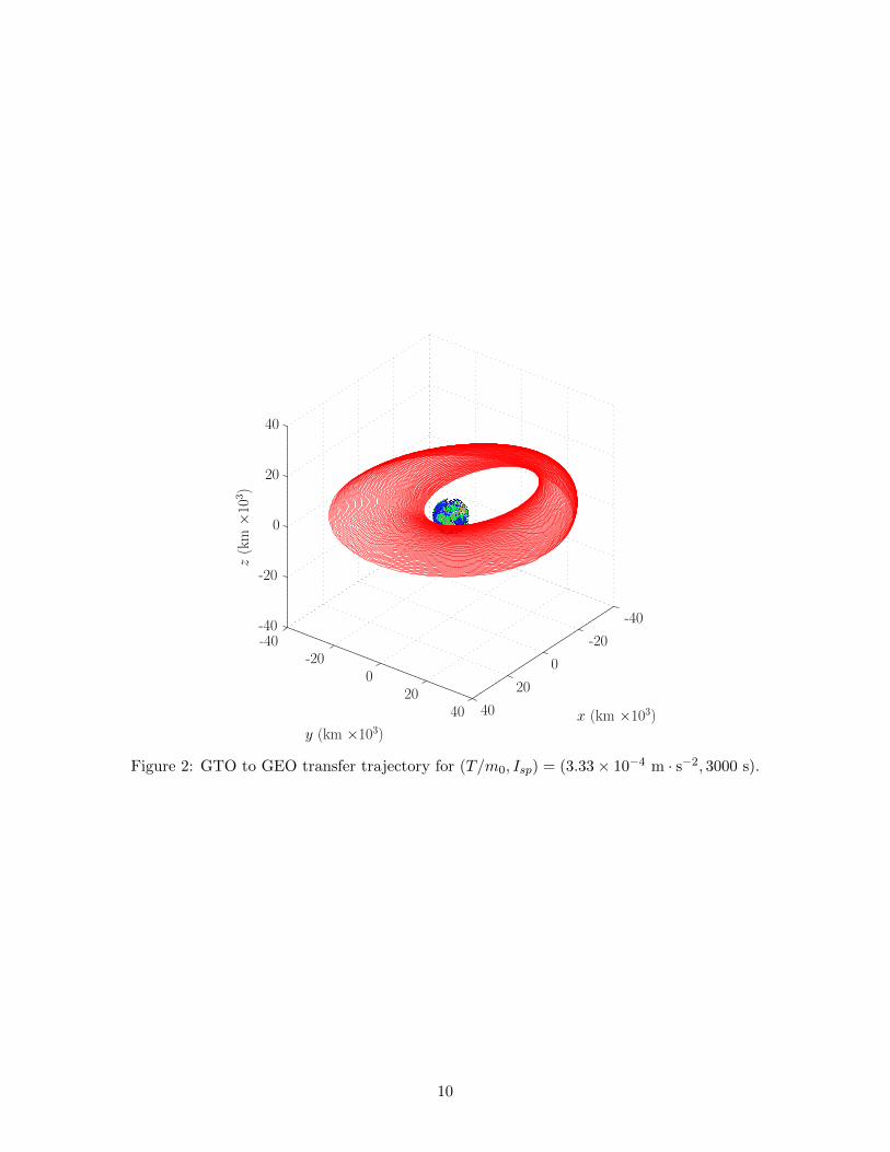
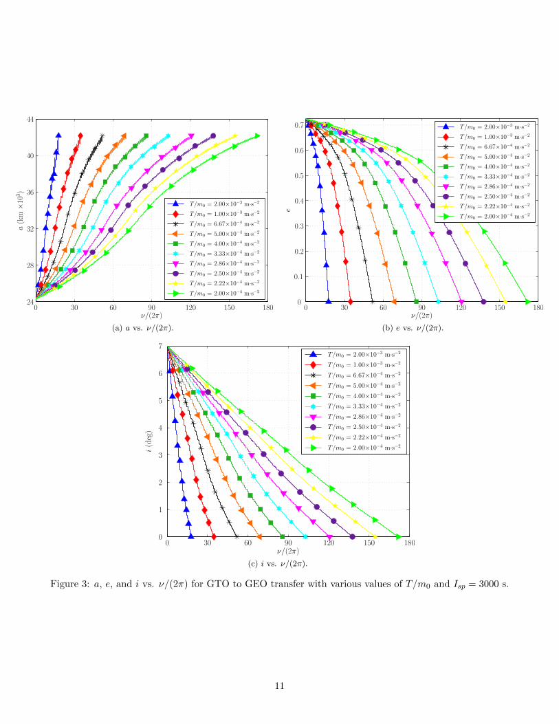
Figure 2 shows a view in Earth-centered inertial Cartesian coordinates (x, y, z) of a typical optimal GTO toGEO trajectory for the case (T/m0, Isp) = (3.33× 10−4 m·s−2, 3000 s). The optimal solution has a 7.78%change in mass, a duration of 74 days, and nearly 103 orbital revolutions. It is seen from Fig. 3a that thesemi-major axis increases nearly linearly throughout the entire transfer, and this rate of increase variesonly slightly as a function of T/m0. Furthermore, Fig. 3b shows that the eccentricity decreases slowly nearthe start of the transfer and decreases more rapidly starting from approximately one third of the way intothe transfer and beyond. Also, Fig. 3c shows that the inclination decreases at an approximately linear ratethroughout the entire transfer.

9

-40-40

-40

-20

-20-20

0

00

20

20 20

40

40 40 x (km ×103)y (km ×103)

z(km

×10

3)

Figure 2: GTO to GEO transfer trajectory for (T/m0, Isp) = (3.33× 10−4 m · s−2, 3000 s).

10

T/m0 = 2.00×10−3 m·s−2

T/m0 = 1.00×10−3 m·s−2

T/m0 = 6.67×10−4 m·s−2

T/m0 = 5.00×10−4 m·s−2

T/m0 = 4.00×10−4 m·s−2

T/m0 = 3.33×10−4 m·s−2

T/m0 = 2.86×10−4 m·s−2

T/m0 = 2.50×10−4 m·s−2

T/m0 = 2.22×10−4 m·s−2

T/m0 = 2.00×10−4 m·s−2

44

40

36

32

28

240 30 60 90 120 150 180

ν/(2π)

a(km

×10

3)

(a) a vs. ν/(2π).

T/m0 = 2.00×10−3 m·s−2

T/m0 = 1.00×10−3 m·s−2

T/m0 = 6.67×10−4 m·s−2

T/m0 = 5.00×10−4 m·s−2

T/m0 = 4.00×10−4 m·s−2

T/m0 = 3.33×10−4 m·s−2

T/m0 = 2.86×10−4 m·s−2

T/m0 = 2.50×10−4 m·s−2

T/m0 = 2.22×10−4 m·s−2

T/m0 = 2.00×10−4 m·s−2

0

0.1

0.2

0.3

0.4

0.5

0.6

0.7

0 30 60 90 120 150 180ν/(2π)

e

(b) e vs. ν/(2π).

T/m0 = 2.00×10−3 m·s−2

T/m0 = 1.00×10−3 m·s−2

T/m0 = 6.67×10−4 m·s−2

T/m0 = 5.00×10−4 m·s−2

T/m0 = 4.00×10−4 m·s−2

T/m0 = 3.33×10−4 m·s−2

T/m0 = 2.86×10−4 m·s−2

T/m0 = 2.50×10−4 m·s−2

T/m0 = 2.22×10−4 m·s−2

T/m0 = 2.00×10−4 m·s−2

0

1

2

3

4

5

6

7

0 30 60 90 120 150 180ν/(2π)

i(deg)

(c) i vs. ν/(2π).

Figure 3: a, e, and i vs. ν/(2π) for GTO to GEO transfer with various values of T/m0 and Isp = 3000 s.

11

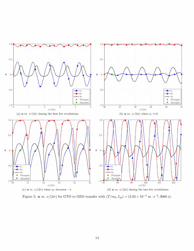
Further insight into the behavior of the optimal GTO to GEO transfers is obtained by examining thecontrol u = (ur, uθ, uh) along different segments of the optimal solution. The typical overall behavior ofu is shown in Fig. 4 for (T/m0, Isp) = (3.33 × 10−4 m·s−2, 3000) s. A closer examination of u revealsthat the following four segments identify the key features of the optimal control: (1) the first few orbitalrevolutions of the transfer, (2) the region where ur ≈ 0, (3) the region where uh becomes −1, and (4)the final revolutions of the transfer. First, the effect of the control on the optimal trajectory in the firstfew orbital revolutions, can be explained via the following differential equations for the semi-major axis,eccentricity, and inclination:37

da

dt=

2e sin ν

nxur +

2ax

nruθ, (24)

de

dt=

x sin ν

naur +

x

na2e

(a2x2

r− r)uθ, (25)

di

dt=

r cos(ν + ω)

na2xuh, (26)

where n is the mean motion and x =√

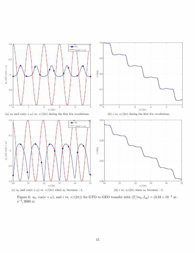
1− e2. It is seen from Eq. (24) that the semi-major axis will increasewhen the control points either in the positive uθ-direction, radially outward near ν = π/2 (halfway betweenperiapsis and apoapsis), or radially inward near ν = 3π/2 (halfway between apoapsis and periapsis).Furthermore, this cyclic behavior of ur increases apoapsis and decreases periapsis when ν ∈ [0, π] anddecreases apoapsis and increases periapsis when ν ∈ [π, 2π]. Equivalently, thrusting radially in this mannerincreases both the semi-major axis and the eccentricity. On the other hand, from Eq. (25) the eccentricitywill decrease when the control points either in the positive uθ-direction, radially inward near ν = π/2, orradially outward near ν = 3π/2. It is seen from Fig. 5a that ur is positive near ν = π/2 and negative nearν = 3π/2, while uθ ≈ 1 in both cases. Even though ur increases the semi-major axis, it simultaneouslyincreases eccentricity. This small effect of ur increasing eccentricity, however, is negated by the fact that ulies predominantly in the positive uθ-direction, thereby resulting in an overall increase in semi-major axisand decrease in eccentricity. Lastly, it is seen from Eq. (26) that di/dt is most negative when cos(ν+ω)uhis most negative. Examining Fig. 6a, it is seen that uh is most positive and cos(ν + ω) = −1 when thespacecraft is at apoapsis, thereby resulting in the largest negative slope in di/dt as seen in Fig. 6b.

Next, Fig. 5b shows u in the segment of an optimal GTO to GEO transfer where ur ≈ 0. Forevery orbital revolution on the optimal solution beyond where ur becomes zero (that is, all values beyondν/(2π) = 38.5 as shown in Fig. 5b), u points radially inward near ν = π/2 such that apoapsis decreases andperiapsis increases when ν ∈ [0, π] and points radially outward near ν = 3π/2 such that apoapsis increasesand periapsis decreases when ν ∈ [π, 2π]. Thrusting radially in this manner decreases both the semi-majoraxis and eccentricity. Although ur decreases the semi-major axis, the thrust direction lies predominantly inthe positive uθ-direction, thereby increasing the semi-major axis and decreasing the eccentricity. Finally,because uh is most positive near ν = π and cos(ν + ω) = −1, the inclination decreases most rapidly nearapoapsis.

Next, Fig. 5c shows u in the segment of an optimal GTO to GEO transfer where uh drops to −1. It isseen in this segment that ur continues to point inward near ν = π/2 and outward near ν = 3π/2, decreasingboth the semi-major axis and the eccentricity. Moreover, uθ no longer dominates the thrust direction,reaching its most positive value at apoapsis and a gradually decreasing value at periapsis. Thrustingin this manner in the ur- and uθ-directions raises periapsis when ν ∈ [0, π] and lowers apoapsis whenν ∈ [π, 2π]. Consequently, the semi-major axis increases while eccentricity decreases. Lastly, from Fig. 6c,uh attains its most negative value near ν = π and cos(ν + ω) = −1 and near ν = 2π and cos(ν + ω) = +1.While the inclination continues to decrease significantly near apoapsis of the transfer, Fig. 6d shows thatdi/dt is also negative near periapsis.

Finally, Fig. 5d shows u during the final few revolutions of an optimal GTO to GEO transfer. It isseen that ur is negative near ν = π/2 and positive near ν = 3π/2, while uθ is positive near ν = 2π and isnegative near ν = π. Consequently, by thrusting in this manner periapsis increases and apoapsis decreases,

12

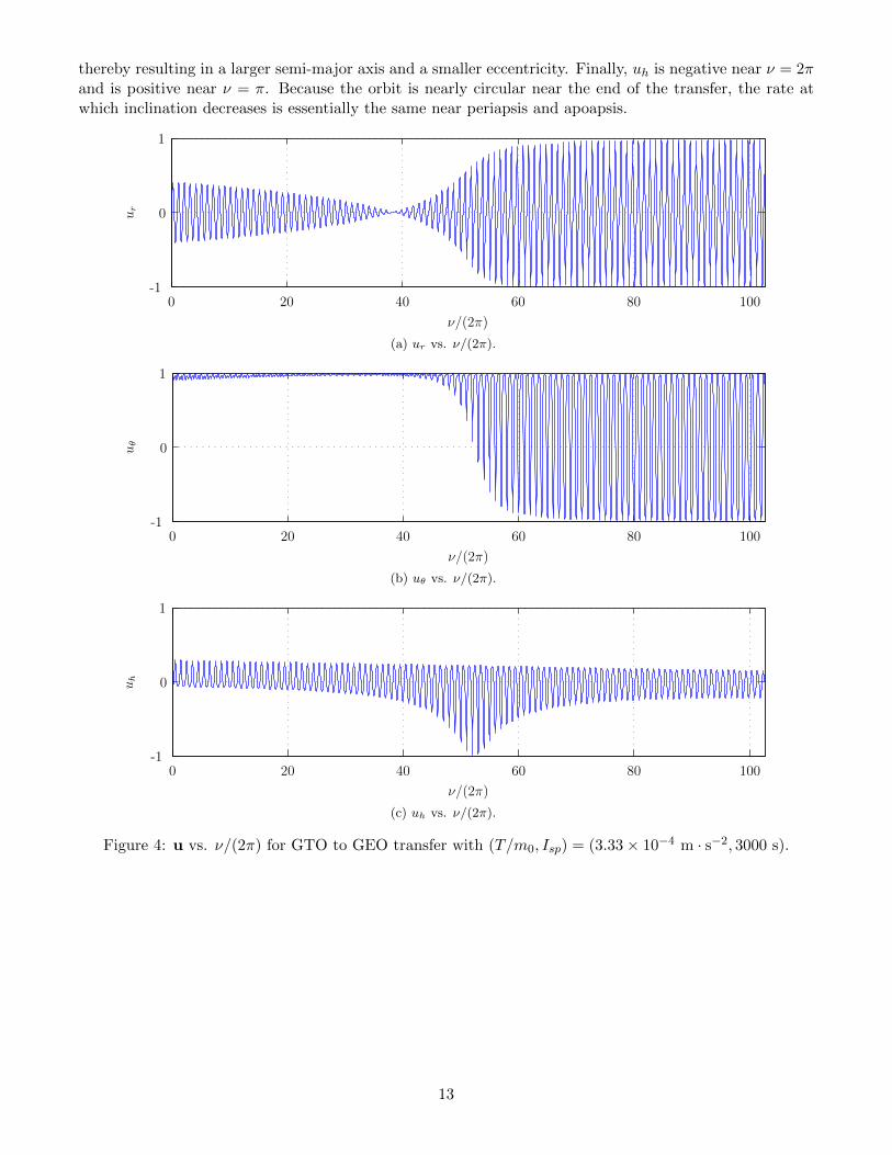
thereby resulting in a larger semi-major axis and a smaller eccentricity. Finally, uh is negative near ν = 2πand is positive near ν = π. Because the orbit is nearly circular near the end of the transfer, the rate atwhich inclination decreases is essentially the same near periapsis and apoapsis.

1

0

0-1

20 40 60 80 100

ν/(2π)

ur

(a) ur vs. ν/(2π).

1

0

0-1

20 40 60 80 100

ν/(2π)

uθ

(b) uθ vs. ν/(2π).

1

0

0-1

20 40 60 80 100

ν/(2π)

uh

(c) uh vs. ν/(2π).

Figure 4: u vs. ν/(2π) for GTO to GEO transfer with (T/m0, Isp) = (3.33× 10−4 m · s−2, 3000 s).

13

ν/(2π)

u

uruθuhPeriapsisApoapsis

-1.0

-0.5

0

0.5

1.0

0 1 2 3 4 5

(a) u vs. ν/(2π) during the first few revolutions.

ν/(2π)

u

uruθuhPeriapsisApoapsis

-1.0

-0.5

0

0.5

1.0

36 37 38 39 40 41

(b) u vs. ν/(2π) when ur ≈ 0.

ν/(2π)

u

uruθuhPeriapsisApoapsis

-1.0

-0.5

0

0.5

1.0

50 51 52 53 54 55

(c) u vs. ν/(2π) when uh becomes −1.

ν/(2π)

u

uruθuhPeriapsisApoapsis

-1.0

-0.5

0

0.5

1.0

97 98 99 100 101 102

(d) u vs. ν/(2π) during the last few revolutions.

Figure 5: u vs. ν/(2π) for GTO to GEO transfer with (T/m0, Isp) = (3.33× 10−4 m · s−2, 3000 s).

14

ν/(2π)

uhandcos(ν+ω)

cos(ν + ω)

uh

-1.0

-0.5

0

0.5

1.0

0 1 2 3 4 5

(a) uh and cos(ν + ω) vs. ν/(2π) during the first few revolutions.

ν/(2π)

i(deg)

0 1 2 3 4 56.6

6.7

6.8

6.9

7.0

(b) i vs. ν/(2π) during the first few revolutions.

ν/(2π)

uhandcos(ν+ω)

cos(ν + ω)

uh

-1.0

-0.5

0

0.5

1.0

50 51 52 53 54 55

(c) uh and cos(ν + ω) vs. ν/(2π) when uh becomes −1.

ν/(2π)

i(deg)

50 51 52 53 54 552.90

3.05

3.20

3.35

(d) i vs. ν/(2π) when uh becomes −1.

Figure 6: uh, cos(ν + ω), and i vs. ν/(2π)) for GTO to GEO transfer with (T/m0, Isp) = (3.33× 10−4 m ·s−2, 3000 s).

15

4.2 Key Features of Optimal LEO to GEO Transfers

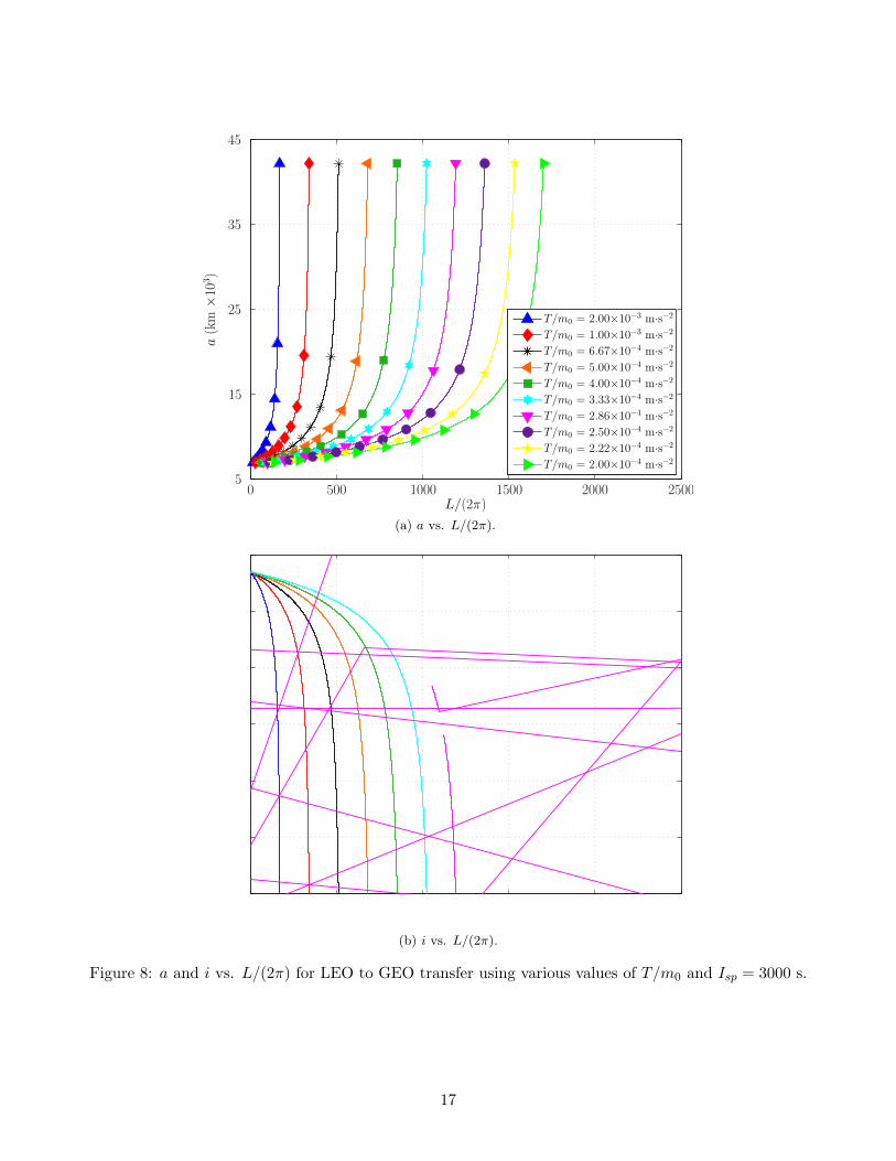
Figure 7 shows a three-dimensional view in Earth-centered inertial Cartesian coordinates (x, y, z) of atypical optimal LEO to GEO trajectory for the case (T/m0, Isp) = (3.33 × 10−4 m·s−2, 1000 s). Theoptimal trajectory has a 44.73% change in mass, takes approximately 152 days, and contains nearly 1,023revolutions. The semi-major axis and inclination for all values of T/m0 and Isp = 1000 s are shown inFigs. 8a and 8b, respectively. It is seen that the semi-major axis increases at a slower rate at the beginningof the transfer and increases more rapidly towards the end of the transfer. The inclination decreases at aslower rate at the beginning of the transfer and decreases more rapidly towards the end of the transfer.The eccentricity is roughly zero throughout the entire transfer.

-50

-50-25

-25

-25

0

00

25

2525

50 50 x (km ×103)

y (km ×103)

z(km

×10

3)

Figure 7: LEO to GEO transfer trajectory with (T/m0, Isp) = (3.33× 10−4 m · s−2, 1000 s).

16

T/m0 = 2.00×10−3 m·s−2

T/m0 = 1.00×10−3 m·s−2

T/m0 = 6.67×10−4 m·s−2

T/m0 = 5.00×10−4 m·s−2

T/m0 = 4.00×10−4 m·s−2

T/m0 = 3.33×10−4 m·s−2

T/m0 = 2.86×10−4 m·s−2

T/m0 = 2.50×10−4 m·s−2

T/m0 = 2.22×10−4 m·s−2

T/m0 = 2.00×10−4 m·s−2

5

15

25

35

45

0 500 1000 1500 2000 2500L/(2π)

a(km

×10

3)

(a) a vs. L/(2π).

T/m0= 2.00×10−3

m·s−2T/m0= 1.00×10−3

m·s−2T/m0= 6.67×10−4m·s− 2T/m0= 5.00×10−4m·s− 2T/m0= 4.00×10−4m·s− 2T/m0= 3.33×10−4m·s− 2T/m0= 2.86×10−4m·s− 2T/m0= 2.50×10−4

m·s−2T/m0= 2.22×10−4

m·s−2T/m0= 2.00×10−4

m·s−2

0

51015

202530

0 500 1000 1500

2000 2500L/( 2π)

i(

deg)

(b) i vs. L/(2π).

Figure 8: a and i vs. L/(2π) for LEO to GEO transfer using various values of T/m0 and Isp = 3000 s.

17

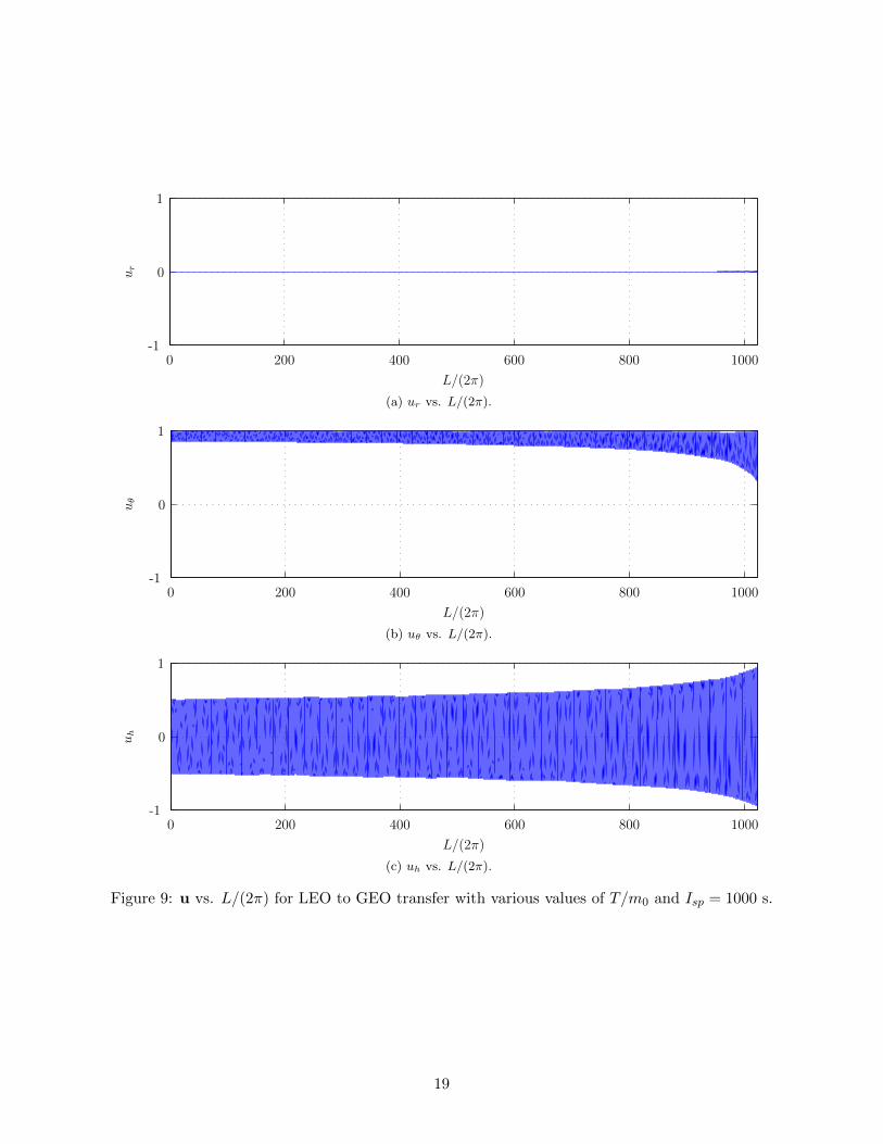
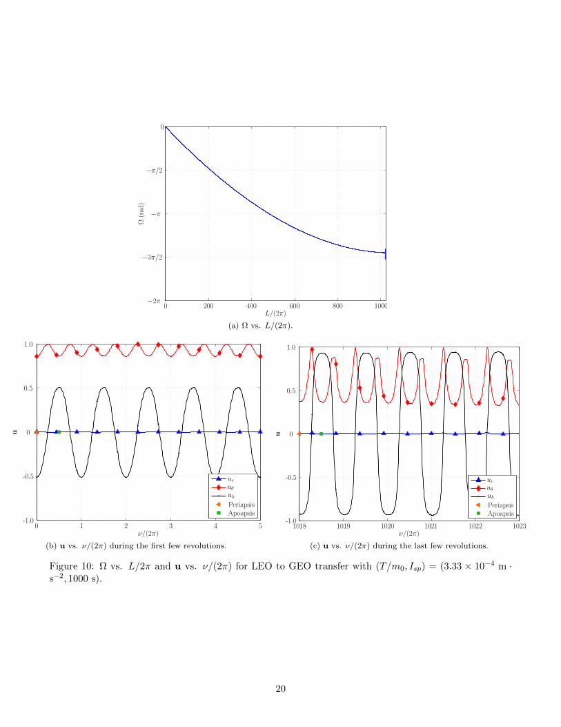
The structure of the optimal LEO to GEO transfers is examined in greater detail by studying thecomponents of the control along the optimal solution. The typical overall behavior of the control u =(ur, uθ, uh) is shown in Fig. 9 for (T/m0, Isp) = (3.33 × 10−4m·s−2, 1000 s). As expected, ur stays nearzero, whereas uθ and uh are non-zero throughout the entire transfer. Greater insight into the structureof the optimal control is now obtained by examining the control near the start and the terminus of thetransfer. Figure 10b shows u as a function of ν near the start of the transfer (where ν = L − Ω − ω ≈ Lbecause L, ω, and Ω, are approximately zero). It is seen from Fig. 10b that uθ points in the positiveuθ-direction to increase the semi-major axis (see Eq. (24)), while uh attains its most positive value nearapoapsis and its most negative value near periapsis to decrease the inclination (see Eq. (26)). Near theterminus of the transfer, ν = L−Ω−ω ≈ L+3π/2 since Ω approaches an approximate value of −3π/2 (seeFig. 10a) and ω is assumed to be zero. Fig. 10c shows u as a function of ν near the end of the transfer whereit is seen that uθ points in the positive uθ-direction and uh attains its most positive value near apoapsisand its most negative value near periapsis. Thus it is clear throughout the LEO to GEO transfer that theoptimal thrust direction increases the semi-major axis and decreases the inclination while the eccentricityremains relatively unchanged near zero.

18

L/(2π)

ur 0

0 200 400 600 800 1000

1

-1

(a) ur vs. L/(2π).

L/(2π)

uθ 0

0 200 400 600 800 1000

1

-1

(b) uθ vs. L/(2π).

L/(2π)

uh 0

0 200 400 600 800 1000

1

-1

(c) uh vs. L/(2π).

Figure 9: u vs. L/(2π) for LEO to GEO transfer with various values of T/m0 and Isp = 1000 s.

19

L/(2π)

Ω(rad)

0

0 200 400 600 800 1000

−π/2

−π

−3π/2

−2π

(a) Ω vs. L/(2π).

ν/(2π)

u

uruθuhPeriapsisApoapsis

-1.0

-0.5

0

0.5

1.0

0 1 2 3 4 5

(b) u vs. ν/(2π) during the first few revolutions.

ν/(2π)

u

uruθuhPeriapsisApoapsis

-1.0

-0.5

0

0.5

1.0

1018 1019 1020 1021 1022 1023

(c) u vs. ν/(2π) during the last few revolutions.

Figure 10: Ω vs. L/2π and u vs. ν/(2π) for LEO to GEO transfer with (T/m0, Isp) = (3.33 × 10−4 m ·s−2, 1000 s).

20

4.3 Estimation of Minimum-Time Transfer Time

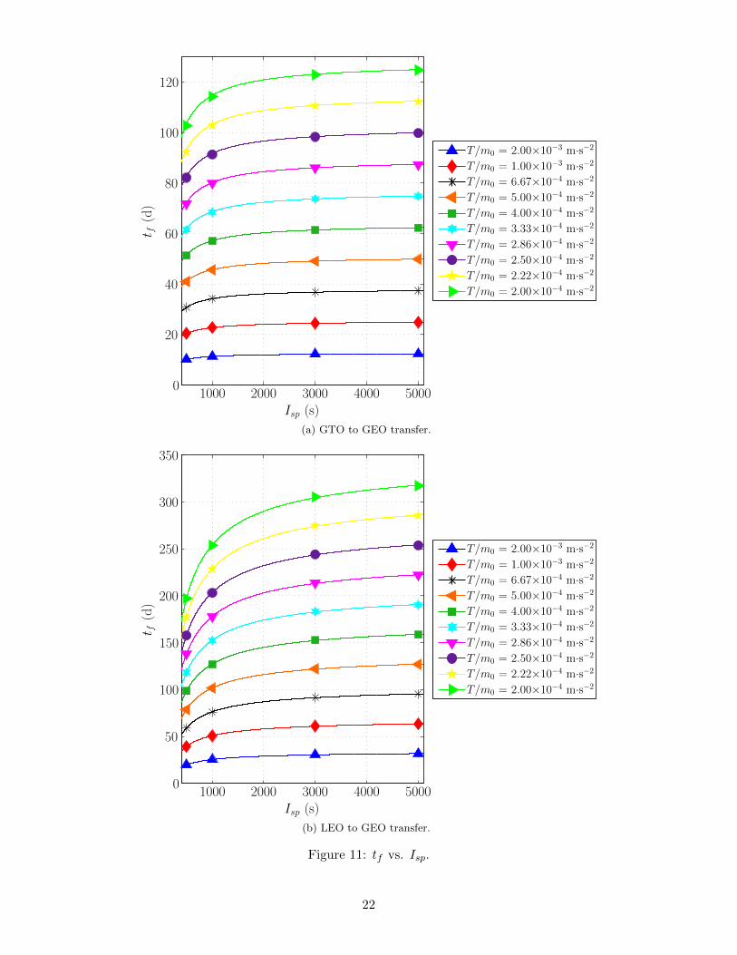
A key feature of the results is the ability to estimate the optimal transfer time as a function of initialthrust acceleration and specific impulse. Figure 11 shows the final time of the orbit transfer as a functionof the specific impulse for each of the initial thrust acceleration values examined. For each value of T/m0,tf increases slightly as Isp increases in a manner similar to that of a power function

tf = AIBsp + C, (27)

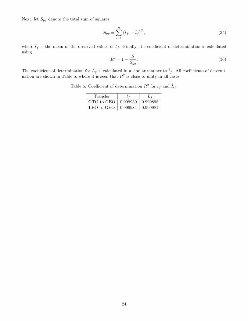
where the coefficients A, B, and C are functions of T/m0 because each value of T/m0 has an associatedpower function expression for tf in terms of Isp. The coefficients A, B, and C are determined as follows.Figures 12a and 12b show the coefficient A as a function of T/m0 for the GTO to GEO and LEO to GEOtransfers, respectively. It is seen that the relationship between A and T/m0 has the form

A = a1(T/m0)b1 , (28)

where a1 and b1 are constant coefficients. Figures 12c and 12d show the coefficient B as a function of T/m0

for the GTO to GEO and LEO to GEO transfers, respectively. Because B has no significant change as afunction of T/m0, it is assumed that B is constant, and for any particular orbital transfer this constantis the average value of B over all values of T/m0 and Isp for that transfer. Figures 12e and 12f show thecoefficient C as a function of T/m0 for the GTO to GEO and LEO to GEO transfers, respectively. It isseen that the relationship between C and T/m0 is given as

C = a2(T/m0)b2 , (29)

where a2 and b2 are constants. Therefore, the estimated transfer time, tf , can be written as a function ofboth Isp and T/m0 and is given as

tf = a1(T/m0)b1(Isp)B + a2(T/m0)b2 . (30)

Values for the coefficients a1, b1, B, a2, and b2 are shown in Table 3. Equation 30 makes it possible toestimate the final transfer time, tf , for values of Isp that are different from those obtained in this studywithout having to re-solve the optimal control problem.

21

Isp (s)

t f(d)

T/m0 = 2.00×10−3 m·s−2

T/m0 = 1.00×10−3 m·s−2

T/m0 = 6.67×10−4 m·s−2

T/m0 = 5.00×10−4 m·s−2

T/m0 = 4.00×10−4 m·s−2

T/m0 = 3.33×10−4 m·s−2

T/m0 = 2.86×10−4 m·s−2

T/m0 = 2.50×10−4 m·s−2

T/m0 = 2.22×10−4 m·s−2

T/m0 = 2.00×10−4 m·s−2

1000 2000 3000 4000 50000

20

40

60

80

100

120

(a) GTO to GEO transfer.

Isp (s)

t f(d)

T/m0 = 2.00×10−3 m·s−2

T/m0 = 1.00×10−3 m·s−2

T/m0 = 6.67×10−4 m·s−2

T/m0 = 5.00×10−4 m·s−2

T/m0 = 4.00×10−4 m·s−2

T/m0 = 3.33×10−4 m·s−2

T/m0 = 2.86×10−4 m·s−2

T/m0 = 2.50×10−4 m·s−2

T/m0 = 2.22×10−4 m·s−2

T/m0 = 2.00×10−4 m·s−2

1000 2000 3000 4000 50000

50

100

150

200

250

300

350

(b) LEO to GEO transfer.

Figure 11: tf vs. Isp.

22

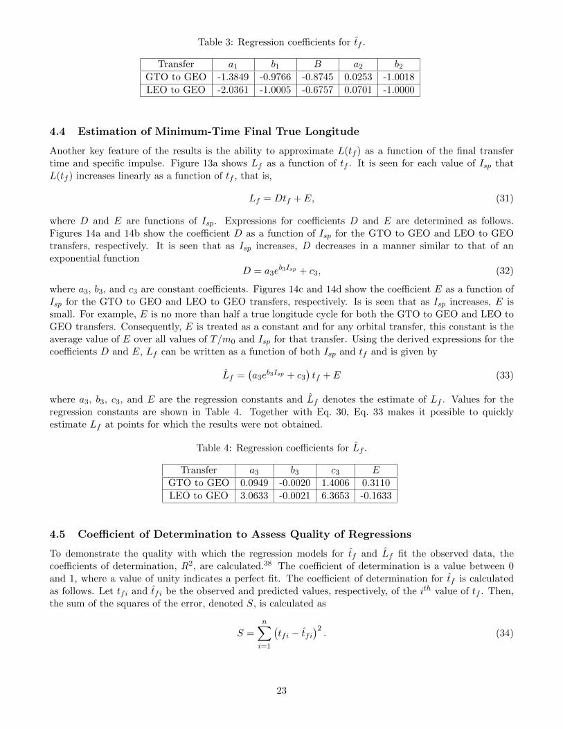
Table 3: Regression coefficients for tf .

Transfer a1 b1 B a2 b2GTO to GEO -1.3849 -0.9766 -0.8745 0.0253 -1.0018

LEO to GEO -2.0361 -1.0005 -0.6757 0.0701 -1.0000

4.4 Estimation of Minimum-Time Final True Longitude

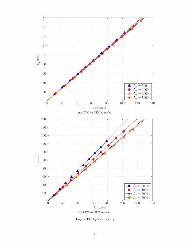
Another key feature of the results is the ability to approximate L(tf ) as a function of the final transfertime and specific impulse. Figure 13a shows Lf as a function of tf . It is seen for each value of Isp thatL(tf ) increases linearly as a function of tf , that is,

Lf = Dtf + E, (31)

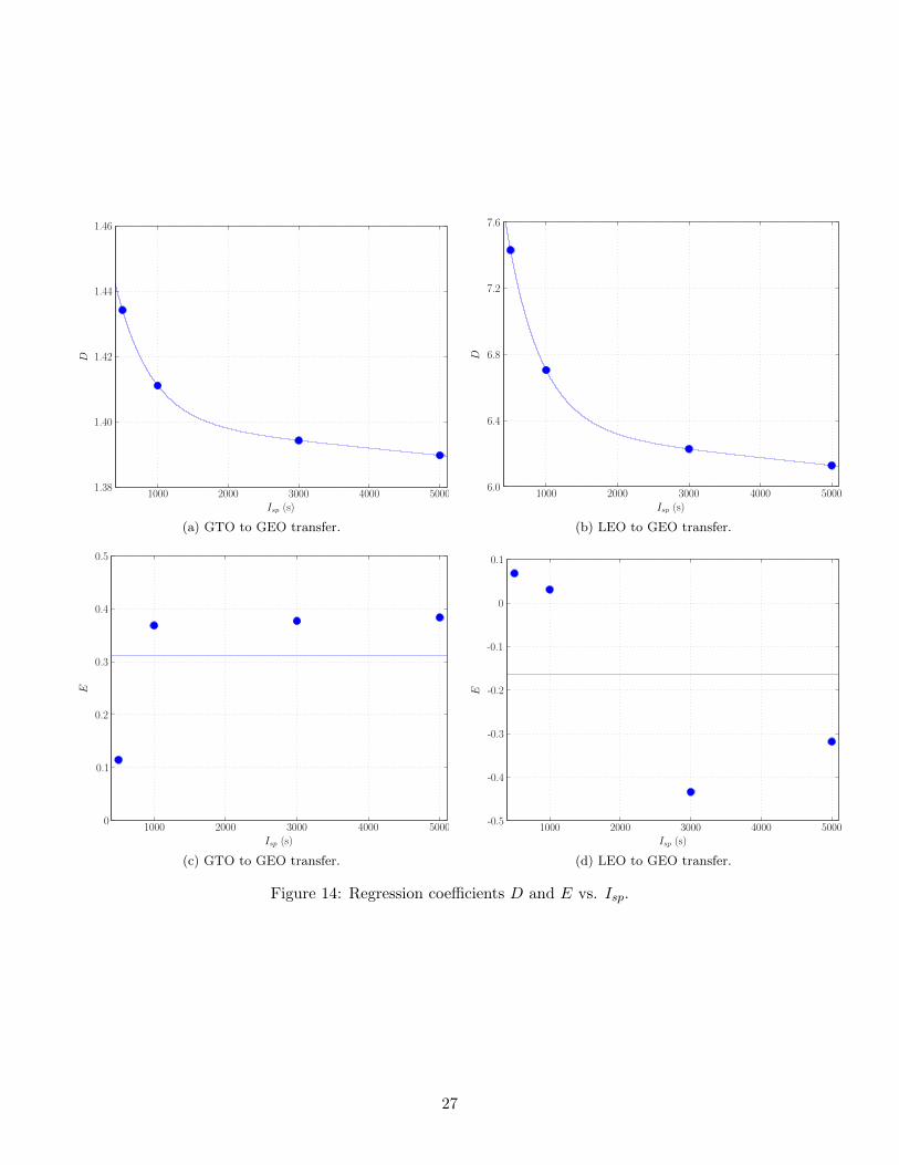
where D and E are functions of Isp. Expressions for coefficients D and E are determined as follows.Figures 14a and 14b show the coefficient D as a function of Isp for the GTO to GEO and LEO to GEOtransfers, respectively. It is seen that as Isp increases, D decreases in a manner similar to that of anexponential function

D = a3eb3Isp + c3, (32)

where a3, b3, and c3 are constant coefficients. Figures 14c and 14d show the coefficient E as a function ofIsp for the GTO to GEO and LEO to GEO transfers, respectively. Is is seen that as Isp increases, E issmall. For example, E is no more than half a true longitude cycle for both the GTO to GEO and LEO toGEO transfers. Consequently, E is treated as a constant and for any orbital transfer, this constant is theaverage value of E over all values of T/m0 and Isp for that transfer. Using the derived expressions for thecoefficients D and E, Lf can be written as a function of both Isp and tf and is given by

Lf =(a3e

b3Isp + c3

)tf + E (33)

where a3, b3, c3, and E are the regression constants and Lf denotes the estimate of Lf . Values for theregression constants are shown in Table 4. Together with Eq. 30, Eq. 33 makes it possible to quicklyestimate Lf at points for which the results were not obtained.

Table 4: Regression coefficients for Lf .

Transfer a3 b3 c3 E

GTO to GEO 0.0949 -0.0020 1.4006 0.3110

LEO to GEO 3.0633 -0.0021 6.3653 -0.1633

4.5 Coefficient of Determination to Assess Quality of Regressions

To demonstrate the quality with which the regression models for tf and Lf fit the observed data, thecoefficients of determination, R2, are calculated.38 The coefficient of determination is a value between 0and 1, where a value of unity indicates a perfect fit. The coefficient of determination for tf is calculatedas follows. Let tfi and tfi be the observed and predicted values, respectively, of the ith value of tf . Then,the sum of the squares of the error, denoted S, is calculated as

S =n∑i=1

(tfi − tfi

)2. (34)

23

Next, let Syy denote the total sum of squares

Syy =n∑i=1

(tfi − tf

)2, (35)

where tf is the mean of the observed values of tf . Finally, the coefficient of determination is calculatedusing

R2 = 1− S

Syy. (36)

The coefficient of determination for Lf is calculated in a similar manner to tf . All coefficients of determi-nation are shown in Table 5, where it is seen that R2 is close to unity in all cases.

Table 5: Coefficient of determination R2 for tf and Lf .

Transfer tf LfGTO to GEO 0.999950 0.999898

LEO to GEO 0.999984 0.999981

24

T/m0 (m·s−2 ×10−3)

A(×

103)

-2

-4

-6

-80 0.5 1.0 1.5 2.0 2.5

0

(a) GTO to GEO transfer.

T/m0 (m·s−2 ×10−3)

A(×

103)

-4

-8

-120 0.5 1.0 1.5 2.0 2.5

0

(b) LEO to GEO transfer.

T/m0 (m·s−2 ×10−3)

B

0 0.5 1.0 1.5 2.0 2.5

-0.82

-0.86

-0.90

-0.94

(c) GTO to GEO transfer.

T/m0 (m·s−2 ×10−3)

B

0 0.5 1.0 1.5 2.0 2.5-0.678

-0.676

-0.674

-0.672

(d) LEO to GEO transfer.

T/m0 (m·s−2 ×10−3)

C

0 0.5 1.0 1.5 2.0 2.5

160

120

80

40

0

(e) GTO to GEO transfer.

T/m0 (m·s−2 ×10−3)

C

0 0.5 1.0 1.5 2.0 2.5

400

300

200

100

0

(f) LEO to GEO transfer.

Figure 12: Regression coefficients A, B, and C vs. T/m0.

25

Lf/(2π

)

tf (days)

Isp = 500 sIsp = 1000 sIsp = 3000 sIsp = 5000 s

180

160

140

140

120

120

100

100

80

80

60

60

40

40

20

2000

(a) GTO to GEO transfer.

Lf/(2π

)

tf (days)

Isp = 500 sIsp = 1000 sIsp = 3000 sIsp = 5000 s

100

2000

1800

1600

1400

1200

1000

800

600

400

350300250

200

2001505000

(b) LEO to GEO transfer.

Figure 13: Lf/(2π) vs. tf .

26

D

Isp (s)1000 2000 3000 4000 5000

1.38

1.40

1.42

1.44

1.46

(a) GTO to GEO transfer.

D

Isp (s)1000 2000 3000 4000 5000

6.0

6.4

6.8

7.2

7.6

(b) LEO to GEO transfer.

E

Isp (s)1000 2000 3000 4000 5000

0.5

0.4

0.3

0.2

0.1

0

(c) GTO to GEO transfer.

E

Isp (s)1000 2000 3000 4000 5000

0.1

0

-0.1

-0.2

-0.3

-0.4

-0.5

(d) LEO to GEO transfer.

Figure 14: Regression coefficients D and E vs. Isp.

27

4.6 Post-Optimality Analysis

It is known from previous research (see Refs. 26 and 27) that the first-order optimality conditions of thenonlinear programming problem arising from discretization of a continuous optimal control problem via theLGR collocation method are a discrete approximation of the first-order calculus of variations optimalityconditions of the optimal control problem. Moreover, the costate of the optimal control problem canbe obtained via a simple linear transformation of the Lagrange multipliers of the NLP arising from theLGR collocation. In addition to the equivalence between the NLP and calculus of variations optimalityconditions, it has also been proven that the solution obtained using the variable-order (hp) LGR collocationmethod converges exponentially (that is, the state, control, and costate associated with the LGR collocationmethod all converge) at the convergence rate given in Ref. 39. Consequently, by solving the NLP arisingfrom the LGR collocation method on an appropriate mesh, an accurate approximation to the solutionof the optimal control problem is obtained to both the primal variables (that is, the state and control)and the dual variable (that is, the costate). Therefore by solving the variable-order LGR NLP on asufficiently accurate mesh, it is possible to verify the extremality of the solutions without having to solvethe Hamiltonian boundary-value problem that arises from the calculus of variations. In other words, byobtaining the solution to the variable-order LGR NLP on an appropriate mesh the optimality of the solutioncan be verified without having to resort to solving the optimal control problem using an indirect method.

In this study the proximity of the numerical solutions to the true optimal solutions is investigated byexamining various aspects of the first-order calculus of variations conditions. In this analysis the first-order variational conditions are presented in terms of the classical orbital elements (as opposed to themodified equinoctial elements which were used to solve the optimal control problem), where the first-order optimality conditions are obtained in terms of the classical orbital elements as follows. First, thediscrete approximation of the costate in terms of the modified equinoctial elements are obtained using thetransformation of the NLP Lagrange multipliers as described in Refs. 26 and 27 (where it is noted thatGPOPS− II performs this costate computation after the NLP is solved). Next, the costate approximationin terms of the modified equinoctial elements obtained from the LGR collocation method is transformedto the costate in terms of classical orbital elements using the relationship between the modified equinoctialelement costate and the classical orbital element costate as derived in the Appendix. Then, using thefact that the costate is the sensitivity of the cost with respect to the state along the optimal solution, thecostate in terms of classical orbital elements at the initial time is also approximated by solving the optimalcontrol problem at a perturbed initial orbital element and taking the ratio of the change in cost to thechange in the orbital element of interest (for example, if it is interested in computing the costate associatedwith the eccentricity, then the ratio of the change in the cost to a perturbation in the eccentricity at theinitial point is computed).

The costates associated with the classical orbital elements of interest were verified by resolving theproblem with a small perturbation in the initial semi-major axis, initial eccentricity, and initial inclination.For a perturbation in the initial semi-major axis, the change in cost from the optimal cost is approximatedas

Jδ ≈ J∗ +

[∂J

∂a(L0)

]∗

(aδ(L0)− a∗(L0)

)(37)

where Jδ and J∗ denote the cost on the perturbed and optimal solutions, respectively. Therefore, theestimated semi-major axis costate at L = L0 is approximated by[

∂J

∂a(L0)

]∗≈ Jδ − J∗aδ(L0)− a∗(L0)

=∆J

∆a(38)

which is then compared to the derived costate value, λ∗a(L0). For a perturbation in the initial eccentricityor initial inclination, the estimated costate value is calculated in a similar manner (that is, replace thesemi-major axis, a, with either the eccentricity, e, or the inclination, i, in Eqs. (37) and (38)). In thisanalysis, the perturbations in the initial semi-major axis, initial eccentricity, and initial inclination were

28

∆a = 1000 m, ∆e = 0.0001 and ∆i = 0.00017453 rad (= 0.01 deg), respectively. Tables 6a and 6b showthe costate approximations (λ∗a(L0), λ∗e(L0), λ∗i (L0)) alongside the ratios of the cost to the perturbations,(∆J/∆a,∆J/∆e,∆J/∆i) in the orbital elements for the GTO to GEO case with T/m0 = 2.22 × 10−4

m·s−2 and for the LEO to GEO case with T/m0 = 4.00 × 10−4 m·s−2. For both cases the LGR costateapproximations closely match the estimated change in cost due to a perturbation in the classical orbitalelement of interest, and the costate approximations are consistent with the expected behavior (for example,increasing the initial semi-major axis for either orbit transfer decreases the cost, while increasing the initialeccentricity increases the cost). Moreover, it is seen that perturbing the initial eccentricity significantlyincreases the cost for the GTO to GEO case but increases the cost much less for the LEO to GEO case.Also, in all cases increasing the initial inclination increases the cost. Finally, in all cases the magnitude ofcost sensitivity increases as the specific impulse increases. This last result is consistent with the fact thatthe efficiency of the engine increases as the specific impulse increases.

As a further verification of the close proximity of the numerical solutions to the true optimal solution,the final column of Tables 6a and 6b show the maximum absolute value of Hu ≡ ∂H/∂u = (Hur ,Huθ ,Huh)on L ∈ [L0, Lf ], that is, Tables 6a and 6b show

maxL∈[L0,Lf ]

(|Hur |, |Huθ |, |Huh |),

where H is computed as given in the Appendix using the costate approximation obtained from the LGRcollocation method as described in Ref. 27. Because the control lies on the interior of the allowable controlset for the problem studied in this paper, it is known theoretically that Hu is zero along the optimalsolution. Commensurate with this known value of Hu, Tables 6a and 6b show that Hu is extremely small,further substantiating the close proximity of the numerical solution to the true optimal solution.

Table 6: Post-optimality results for GTO to GEO and LEO to GEO transfers.

(a) GTO to GEO post-optimality results for T/m0 = 2.50 × 10−4 m·s−2.

Isp λ∗a(t0) ∆J/∆a λ∗e(t0) ∆J/∆e λ∗i (t0) ∆J/∆i maxL∈[L0,Lf ]

(|Hur |, |Huθ |, |Huh |)

500 -1.84×10−6 -1.84×10−6 77.78 77.81 17.45 17.47 2.65×10−9

1000 -2.31×10−6 -2.30×10−6 97.58 97.70 21.92 21.98 3.33×10−10

3000 -2.39×10−6 -2.39×10−6 108.74 108.69 24.45 24.47 2.20×10−10

5000 -2.75×10−6 -2.75×10−6 116.72 116.78 26.24 26.27 2.22×10−10

(b) LEO to GEO post-optimality results for T/m0 = 4.00 × 10−4 m·s−2.

Isp λ∗a(t0) ∆J/∆a λ∗e(t0) ∆J/∆e λ∗i (t0) ∆J/∆i maxL∈[L0,Lf ]

(|Hur |, |Huθ |, |Huh |)

500 -4.73×10−6 -4.72×10−6 0.14 0.14 36.75 36.75 1.53×10−10

1000 -8.56×10−6 -8.53×10−6 0.40 0.40 66.57 66.58 1.67×10−10

3000 -1.30×10−5 -1.29×10−5 0.59 0.59 99.20 99.22 1.42×10−10

5000 -1.38×10−5 -1.37×10−5 0.63 0.57 107.06 107.04 2.08×10−10

29

5 Conclusions

The problem of high-accuracy low-thrust minimum-time Earth-orbit transfers has been studied. Theoptimal orbital transfer problem is posed as a constrained nonlinear optimal control problem. It is solvedusing a variable-order Legendre-Gauss-Radau (LGR) quadrature orthogonal collocation method pairedwith a search method that helps the NLP solver determine the best locally optimal solution. A numericaloptimization study has been conducted to determine optimal trajectories and controls for a range of initialthrust accelerations and constant specific impulses. The key features of the solutions have been identifiedand relationships have been obtained that relate the optimal transfer time to the optimal number oftrue longitude cycles as a function of the initial thrust acceleration and specific impulse. Finally, a post-optimality analysis has been performed that verifies the optimality of the solutions that were obtained inthis study.

Acknowledgments

The authors gratefully acknowledge support for this research by the NASA Florida Space Grant Consortiumunder grant NNX10AM01H, by Space Florida under grant 11-107, and by the National Aeronautics andSpace Administration under grant NNX14AN88G.

References

[1] Dachwald, B., “Optimization of Very-Low-Thrust Trajectories Using Evolutionary Neurocontrol,”Acta Astronautica, Vol. 57, No. 2-8, 2005, pp. 175–185.

[2] Tang, S. and Conway, B. A., “Optimization of Low-Thrust Interplanetary Trajectories Using Collo-cation and Nonlinear Programming,” Journal of Guidance, Control, and Dynamics, Vol. 18, No. 3,May-June 1995, pp. 599–604.

[3] Rauwolf, G. A. and Coverstone-Carroll, V. L., “Near-Optimal Low-Thrust Orbit Transfers Generatedby a Genetic Algorithm,” Journal of Spacecraft and Rockets, Vol. 33, No. 6, November-December1996, pp. 859–862.

[4] Coverstone-Carroll, V., Hartmann, J. W., and Mason, W. J., “Optimal Multi-Objective Low-ThrustSpacecraft Trajectories,” Computer Methods in Applied Mechanics and Engineering , Vol. 186, No.2-4, June 2000, pp. 387–402.

[5] Falck, R. D. and Dankanich, J. D., “Optimization of Low-Thrust Spiral Trajectories by Collocation,”AIAA/AAS Astrodynamics Specialist Conference, No. 2012-4423, Minneapolis, MN, August 2012.

[6] Petropoulos, A. and Longuski, J. M., “Shaped-Based Algorithm for the Automated Design of Low-Thrust, Gravity Assist Trajectories,” Journal of Spacecraft and Rockets, Vol. 41, No. 5, September-October 2004, pp. 787–796.

[7] Starek, J. A. and Kolmanovsky, I. V., “Nonlinear model predictive control strategy for low thrustspacecraft missions,” Optimal Control Applications and Methods, Vol. 35, No. 1, January-February2014, pp. 1–20.

[8] Bartholomew-Biggs, M. C., Dixon, L. C. W., Hersom, S. E., and Maany, Z. A., “The solution of somedifficult problems in low-thrust interplanetary trajectory optimization,” Optimal Control Applicationsand Methods, Vol. 9, No. 3, July-September 1988, pp. 229–251.

[9] Kechichian, J. A., “Optimal Low-Thrust Transfers Using Variable Bounded Thrust,” Acta Astronau-tica, Vol. 36, No. 7, 1995, pp. 357–365.

30

[10] da Silva Fernandes, S., “Optimum Low-Thrust Limited Power Transfers Between Neighbouring EllipticNon-Equatorial Orbits in a Non-Central Gravity Field,” Acta Astronautica, Vol. 35, No. 12, 1995,pp. 763–770.

[11] Pontryagin, L. S., Boltyanskii, V. G., Gamkrelidze, R., and Mishchenko, E. F., The MathematicalTheory of Optimal Processes (Russian), English Translation: Interscience, 1962.

[12] Athans, M. A. and Falb, P. L., Optimal Control: An Introduction to the Theory and Its Applications,Dover Publications, Mineola, New York, 2006.

[13] Alfano, S. and Thorne, J. D., “Circle-to-Circle, Constant-Thrust Orbit Raising,” The Journal ofAstronautical Sciences, Vol. 42, No. 1, 1994, pp. 35–45.

[14] Haissig, C. M., Mease, K. D., and Vinh, N. X., “Minimum-Fuel, Power-Limited Transfers BetweenCoplanar Elliptic Orbits,” Acta Astronautica, Vol. 29, No. 1, January 1993, pp. 1–15.

[15] Kluever, C. A. and Oleson, S. R., “Direct Approach for Computing Near-Optimal Low-Thrust Earth-Orbit Transfers,” Journal of Spacecraft and Rockets, Vol. 35, No. 4, July-August 1998, pp. 509–515.

[16] Yang, G., “Direct Optimization of Low-thrust Many-revolution Earth-orbit Transfers,” Chinese Jour-nal of Aeronautics, Vol. 22, No. 4, August 2009, pp. 426–433.

[17] Scheel, W. A. and Conway, B. A., “Optimization of Very-Low-Thrust, Many-Revolution SpacecraftTrajectories,” Journal of Guidance, Control, and Dynamics, Vol. 17, No. 6, November-December 1994,pp. 1185–1192.

[18] Haberkorn, T., Martinon, P., and Gergaud, J., “Low-Thrust Minimum-Fuel Orbital Transfer: AHomotopic Approach,” Journal of Guidance, Control, and Dynamics, Vol. 27, No. 6, 2004.

[19] Betts, J. T., “Very Low-Thrust Trajectory Optimization Using a Direct SQP Method,” Journal ofComputational and Applied Mathematics, Vol. 120, No. 1-2, August 2000, pp. 27–40.

[20] Ross, I. M., Gong, Q., and Sekhavat, P., “Low-Thrust, High-Accuracy Trajectory Optimization,”Journal of Guidance, Control, and Dynamics, Vol. 30, No. 4, July-August 2007, pp. 921–933.

[21] Schubert, K. F. and Rao, A. V., “Minimum-Time Low-Earth Orbit to High-Earth Orbit Low-ThrustTrajectory Optimization,” AAS/AIAA Astrodynamics Specialist Conference, No. 12-926, Hilton Head,SC, August 2013.

[22] Benson, D. A., Huntington, G. T., Thorvaldsen, T. P., and Rao, A. V., “Direct Trajectory Optimiza-tion and Costate Estimation via an Orthogonal Collocation Method,” Journal of Guidance, Control,and Dynamics, Vol. 29, No. 6, November-December 2006, pp. 1435–1440.

[23] Huntington, G. T., Benson, D. A., and Rao, A. V., “Optimal Configuration of Tetrahedral SpacecraftFormations,” Journal of the Astronautical Sciences, Vol. 55, No. 2, April-June 2007, pp. 141–169.

[24] Huntington, G. T. and Rao, A. V., “Optimal Reconfiguration of Tetrahedral Spacecraft FormationsUsing the Gauss Pseudospectral Method,” Journal of Guidance, Control, and Dynamics, Vol. 31,No. 3, May-June 2008, pp. 141–169.

[25] Rao, A. V., Benson, D. A., Darby, C. L., Francolin, C., Patterson, M. A., Sanders, I., and Huntington,G. T., “Algorithm 902: GPOPS, A Matlab Software for Solving Multiple-Phase Optimal ControlProblems Using the Gauss Pseudospectral Method,” ACM Transactions on Mathematical Software,Vol. 37, No. 2, April–June 2010, Article 22, 39 pages.

31

[26] Garg, D., Patterson, M. A., Hager, W. W., Rao, A. V., Benson, D. A., and Huntington, G. T., “AUnified Framework for the Numerical Solution of Optimal Control Problems Using PseudospectralMethods,” Automatica, Vol. 46, No. 11, November 2010, pp. 1843–1851.

[27] Garg, D., Patterson, M. A., Darby, C. L., Francolin, C., Huntington, G. T., Hager, W. W., and Rao,A. V., “Direct Trajectory Optimization and Costate Estimation of Finite-Horizon and Infinite-HorizonOptimal Control Problems via a Radau Pseudospectral Method,” Computational Optimization andApplications, Vol. 49, No. 2, June 2011, pp. 335–358.

[28] Patterson, M. A., Hager, W. W., and Rao, A. V., “A ph Mesh Refinement Method for OptimalControl,” Optimal Control Applications and Methods, January 2014, Online in Early View, DOI:10.1002/oca2114.

[29] Patterson, M. A. and Rao, A. V., “GPOPS-II: A MATLAB Software for Solving Multiple-PhaseOptimal Control Problems Using hp-Adaptive Gaussian Quadrature Collocation Methods and SparseNonlinear Programming,” ACM Transactions on Mathematical Software, Vol. 41, No. 1, October 2014,pp. 1:1–1:37.

[30] Walker, M. J. H., Owens, J., and Ireland, B., “A Set of Modified Equinoctial Orbit Elements,” CelestialMechanics, Vol. 36, No. 4, 1985, pp. 409–419.

[31] Prussing, J. E. and Conway, B. A., Orbital Mechanics, Oxford University Press, 2nd ed., 2013.

[32] Patterson, M. A. and Rao, A. V., “Exploiting Sparsity in Direct Collocation Pseudospectral Methodsfor Solving Optimal Control Problems,” Journal of Spacecraft and Rockets, Vol. 49, No. 2, March–April2012, pp. 364–377.

[33] Darby, C. L., Hager, W. W., and Rao, A. V., “Direct Trajectory Optimization Using a Variable Low-Order Adaptive Pseudospectral Method,” Journal of Spacecraft and Rockets, Vol. 48, No. 3, May-June2011, pp. 433–445.

[34] Darby, C. L., Hager, W. W., and Rao, A. V., “An hp-adaptive pseudospectral method for solvingoptimal control problems,” Optimal Control Applications and Methods, Vol. 32, August 2011, pp. 476–502.

[35] Biegler, L. T. and Zavala, V. M., “Large-Scale Nonlinear Programming Using IPOPT: An IntegratingFramework for Enterprise-Wide Optimization,” Computers and Chemical Engineering , Vol. 33, No. 3,March 2008, pp. 575–582.

[36] Weinstein, M. J. and Rao, A. V., “A Source Transformation via Operator Overloading Method for theAutomatic Differentiation of Mathematical Functions in MATLAB,” ACM Transactions on Mathe-matical Software, September 2014, Accepted for Publication.

[37] Chobotov, V. A., Orbital Mechanics, American Institute of Aeronautics and Astronautics, Inc., 1991.

[38] Wackerly, D. D., Mendenhall, W., and Scheaffer, R. L., Mathematical Statistics with Applications,Thomson Brooks/Cole, 7th ed., 2008.

[39] Hou, H., Convergence Analysis of Orthogonal Collocation Methods for Unconstrained Optimal Control ,Ph.d. thesis, University of Florida, Gainesville, Florida, May 2013.

32

6 Appendix

In this Appendix we derive expressions for the components of the costate of the optimal control problem

given Section 2 in terms of the components of the costate in terms of the modified equinoctial elements.

First, the augmented Hamiltonian, H, of the minimum-time optimal control problem described in Section

2 is given in terms of the differential equations in modified equinoctial elements as

H = λpGp + λfGf + λgGg + λhGh + λkGk + λmGm + λtGt − µ(u2r + u2

θ + u2h − 1), (39)

where (λp, λf , λg, λh, λk, λm, λt) is the costate associated with the differential equations of Eqs. (3) and (4)

and µ is the Lagrange multiplier associated with the path constraint of Eq. (17). The Hamiltonian can be

expressed equivalently in terms of the classical orbital elements as

H = λaGa + λeGe + λiGi + λΩGΩ + λωGω + λmGm + λtGt, (40)

where (Ga, Ge, Gi, GΩ, Gω) define the right-hand sides of those components of the equations of motion

given in Eqs. (3) and (4) that correspond to the dynamics for the orbital elements a, e, i, Ω, ω, that is,

da

dL= Ga,

de

dL= Ge,

di

dL= Gi,

dΩ

dL= GΩ,

dω

dL= Gω.

(41)

Because the components of the costate λm and λt are the same using either modified equinoctial elements

or orbital elements and the control is the same in both formulations, the Hamiltonian given in either (39)

or (39) can be replaced with the reduced Hamiltonian,

Hr = λpGp + λfGf + λgGg + λhGh + λkGk,

= λaGa + λeGe + λiGi + λΩGΩ + λωGω.(42)

33

Next, the relationship between the modified equinoctial elements and the classical orbital elements are

given as

a = a(p, f, g) =p

1− f2 − g2

e = e(f, g) =√f2 + g2

i = i(h, k) = tan−1

(2√h2 + k2

1− k2 − h2

)

Ω = Ω(h, k) = tan−1

(k

h

)

ω = ω(f, g, h, k) = tan−1

(gh− fkfh+ gk

).

(43)

The expressions for da/dL, de/dL, di/dL, dΩ/dL, and dω/dL are then given in terms of modified equinoctial

elements as

da

dL=∂a

∂p

dp

dL+∂a

∂f

df

dL+∂a

∂g

dg

dL=∂a

∂pGp +

∂a

∂fGf +

∂a

∂gGg,

de

dL=∂e

∂f

df

dL+∂e

∂g

dg

dL=∂e

∂fGf +

∂e

∂gGg,

di

dL=∂i

∂h

dh

dL+∂i

∂k

dk

dL=∂i

∂hGh +

∂i

∂kGk,

dΩ

dL=∂Ω

∂h

dh

dL+∂Ω

∂k

dk

dL=∂Ω

∂hGh +

∂Ω

∂kGk,

dω

dL=∂ω

∂f

df

dL+∂ω

∂g

dg

dL+∂ω

∂h

dh

dL+∂ω

∂k

dk

dL=∂ω

∂fGf +

∂ω

∂gGg +

∂ω

∂hGh +

∂ω

∂kGk.

(44)

Substituting (44) into (42), the reduced Hamiltonian can be expressed as

Hr = λa

[∂a

∂pGp +

∂a

∂fGf +

∂a

∂gGg

]+ λe

[∂e

∂fGf +

∂e

∂gGg

]+ λi

[∂Ω

∂hGh +

∂Ω

∂kGk

]+ λΩ

[∂Ω

∂hGh +

∂Ω

∂kGk

]+ λω

[∂ω

∂fGf +

∂ω

∂gGg +

∂ω

∂hGh +

∂ω

∂kGk

] (45)

and rearranged to yield

Hr =

[λa∂a

∂p

]Gp +

[λa∂a

∂f+ λe

∂e

∂f+ λω

∂ω

∂f

]Gf +

[λa∂a

∂g+ λe

∂e

∂g+ λω

∂ω

∂g

]Gg

+

[λi∂i

∂h+ λΩ

∂Ω

∂h+ λω

∂ω

∂h

]Gh +

[λi∂i

∂k+ λΩ

∂Ω

∂k+ λω

∂ω

∂k

]Gk

= λpGp + λfGf + λgGg + λhGh + λkGk.

(46)

34

Equating terms in (46) leads to the following system of five linear equations that relate (λa, λe, λi, λΩ, λω)

to (λp, λf , λg, λh, λk):

λp

λf

λg

λh

λk

=

∂a∂p 0 0 0 0

∂a∂f

∂e∂f 0 0 ∂ω

∂f

∂a∂g

∂e∂g 0 0 ∂ω

∂g

0 0 ∂i∂h

∂Ω∂h

∂ω∂h

0 0 ∂i∂k

∂Ω∂k

∂ω∂k

λa

λe

λi

λΩ

λω

(47)

Assuming that the system matrix

∂a∂p 0 0 0 0

∂a∂f

∂e∂f 0 0 ∂ω

∂f

∂a∂g

∂e∂g 0 0 ∂ω

∂g

0 0 ∂i∂h

∂Ω∂h

∂ω∂h

0 0 ∂i∂k

∂Ω∂k

∂ω∂k

is invertible, Eq. (47) can be solved to obtain (λa, λe, λi, λΩ, λω).

35