Embed Size (px)
Citation preview

Noname manuscript No.(will be inserted by the editor)
Mining Closed Strict Episodes?
Nikolaj Tatti and Boris Cule
the date of receipt and acceptance should be inserted later
Abstract Discovering patterns in a sequence is an important aspect of data mining.
One popular choice of such patterns are episodes, patterns in sequential data describing
events that often occur in the vicinity of each other. Episodes also enforce in which
order the events are allowed to occur.
In this work we introduce a technique for discovering closed episodes. Adopting
existing approaches for discovering traditional patterns, such as closed itemsets, to
episodes is not straightforward. First of all, we cannot define a unique closure based
on frequency because an episode may have several closed superepisodes. Moreover, to
define a closedness concept for episodes we need a subset relationship between episodes,
which is not trivial to define.
We approach these problems by introducing strict episodes. We argue that this
class is general enough, and at the same time we are able to define a natural subset
relationship within it and use it efficiently. In order to mine closed episodes we define
an auxiliary closure operator. We show that this closure satisfies the needed properties
so that we can use the existing framework for mining closed patterns. Discovering the
true closed episodes can be done as a post-processing step. We combine these observa-
tions into an efficient mining algorithm and demonstrate empirically its performance
in practice.
Keywords Frequent Episode Mining, Closed Episodes, Level-wise Algorithm
1 Introduction
Discovering frequent patterns in an event sequence is an important field in data mining.
Episodes, as defined in [1212], represent a rich class of sequential patterns, enabling us to
discover events occurring in the vicinity of each other while at the same time capturing
complex interactions between the events.
? A preliminary version appeared as ”Mining Closed Strict Episodes”, in Proceedings ofTenth IEEE International Conference on Data Mining (ICDM 2010), 2010 [1717].
Nikolaj Tatti · Boris CuleUniversity of Antwerp, Antwerp, Belgium,E-mail: [email protected], [email protected]
2
More specifically, a frequent episode is traditionally considered to be a set of events
that reoccurs in the sequence within a window of a specified length. Gaps are allowed
between the events and the order in which the events are allowed to occur is specified
by the episode. Frequency, the number of windows in which the episode occurs, is
monotonically decreasing so we can use the well-known level-wise approach to mine all
frequent episodes.
The order restrictions of an episode are described by a directed acyclic graph
(DAG): the set of events in a sequence covers the episode if and only if each event
occurs only after all its parent events (with respect to the DAG) have occurred (see
the formal definition in Section 22). Usually, only two extreme cases are considered. A
parallel episode poses no restrictions on the order of events, and a window covers the
episode if the events occur in the window, in any order. In such a case, the DAG asso-
ciated with the episode contains no edges. The other extreme case is a serial episode.
Such an episode requires that the events occur in one, and only one, specific order in
the sequence. Clearly, serial episodes are more restrictive than parallel episodes. If a
serial episode is frequent, then its parallel version is also frequent.
The advantage of episodes based on DAGs is that they allow us to capture depen-
dencies between the events while not being too restrictive.
Example 1 As an example we will use text data, namely inaugural speeches by pres-
idents of the United States (see Section 88 for more details). Protocol requires the
presidents to address the chief justice and the vice presidents in their speeches. Hence,
a pattern
chief→ justic vice→ president
occurs in 10 disjoint windows. This pattern captures the phrases ’chief justice’ and ’vice
president’ but because the address order varies from speech to speech, the pattern does
not impose any additional restrictions.
Episodes based on DAGs have, in practice, been over-shadowed by parallel and
serial episodes, despite being defined at the same time [1212]. The main reason for this
is the pattern explosion demonstrated in the following example.
Example 2 To illustrate the pattern explosion we will again use inaugural speeches by
presidents of the United States. By setting the window size to 15 and the frequency
threshold to 60 we discovered a serial episode with 6 symbols,
preserv→ protect→ defend→ constitut→ unit→ state.
In total, we found another 4823 subepisodes of size 6 of this episode. However, all
these episodes had only 3 distinct frequencies, indicating that the frequencies of most
of them could be derived from the frequencies of only 3 episodes, so the output could
be reduced by leaving out 4821 episodes.
We illustrate the pattern explosion further in Table 11. We see from the table that if
the sequence has a frequent serial episode consisting of 9 labels, then mining frequent
episodes will produce at least 100 million patterns.
Motivated by this example, we approach the problem of pattern explosion by using a
popular technique of closed patterns. A pattern is closed if there exists no superpattern
with the same frequency. Mining closed patterns has been shown to reduce the output.
Moreover, we can discover closed patterns efficiently. However, adopting the concept
of closedness to episodes is not without problems.
3
pattern 1 2 3 4 5 6 7 8 9
itemsets 1 3 7 15 31 63 127 255 511episodes 1 4 16 84 652 7 742 139 387 3 730 216 145 605 024
Table 1 Illustration of the pattern explosion. The first row is the number of frequent itemsetsproduced by a single frequent itemset with n items. The second row is the number of episodesproduced by a single frequent serial episode with n unique labels. These numbers were obtainedby a brute force enumeration.
Subset relationship Establishing a proper subset relationship is needed for two rea-
sons. Firstly, to make the mining procedure more efficient by discovering all possible
subpatterns before testing the actual episode, and secondly, to define a proper closure
operator.
A naıve approach to define whether an episode G is a subepisode of an episode
H is to compare their DAGs. This, however, leads to problems as the same episode
can be represented by multiple DAGs and a graph representing G is not necessarily a
subgraph of a graph representing H as demonstrated in the following example.
Example 3 Consider episodes G1, G2, and G3 given in Figure 11. Episode G1 states
that for a pattern to occur a must precede b and c. Meanwhile, G2 and G3 state that
a must be followed by b and then by c. Note that G2 and G3 represent essentially the
same pattern that is more restricted than the pattern represented by G1. However, G1
is a subgraph of G3 but not a subgraph of G2. This reveals a problem if we base our
definition of a subset relationship of episodes solely on the edge subset relationship. We
solve this particular case by considering transitive closures, graphs in which each node
must be connected to all its descendants by an edge, thus ignoring graphs of form G2.
We will not lose any generality since we are still going to discover episodes of form G3.
Using transitive closure does not solve all problems for episodes containing multiple
nodes with the same label. For example, episodes H1 and H2 in Figure 11 are the same
even though their graphs are different.
a
cb
(a) Episode G1
a cb
(b) Episode G2
a
cb
(c) Episode G3
a a
b b
(d) Episode H1
a a
b b
(e) Episode H2
Fig. 1 Toy episodes used in Example 33.
Frequency closure Secondly, frequency does not satisfy the Galois connection. In fact,
given an episode G there can be several more specific closed episodes that have the same
frequency. So the closure operator cannot be defined as a mapping from an episode to
its frequency-closed version.
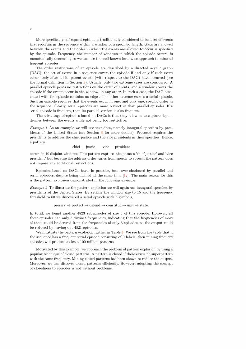
Example 4 Consider sequence s given in Figure 2(e)2(e) and episode G1 given in Fig-
ure 2(a)2(a). Assume that we use a sliding window of size 5. There are two windows that
cover episode G1, namely s[1, 5] and s[6, 10], illustrated in Figure 2(e)2(e). Hence, the fre-
quency of G1 is 2. There are two serial episodes that are more specific than G1 and
4
have the same frequency, namely, G2 and G3 given in Figures 2(b)2(b) and 2(c)2(c). Moreover,
there is no superepisode of G2 and G3 that has frequency equal to 2. In other words,
we cannot define a unique closure for G1 based on frequency.
ac
bd
(a) Episode G1
a cb d
(b) Episode G2
a c b d
(c) Episode G3
a
c b
d
(d) Episode G4
a b c b d a c b c d
(e) Sequence s
Fig. 2 Toy episodes used in Examples 44 and 55. Edges induced by transitive closure are omittedto avoid clutter.
The contributions of our paper address these issues:
1. We introduce strict episodes, a new subclass of general episodes. We say that an
episode is strict if all nodes with the same label are connected. Thus all episodes
in Figure 11 are strict, except H2. We will argue that this class is large, contains all
serial and parallel episodes, as well as episodes with unique labels, yet using only
strict episodes eases the computational burden.
2. We introduce a natural subset relationship between episodes based on the subset
relationship of sequences covering the episodes. We will prove that for strict episodes
this relationship corresponds to the subset relationship between transitively closed
graphs. For strict episodes such a graph uniquely defines the episode.
3. We introduce milder versions of the closure concept, including the instance-closure.
We will show that these closures can be used efficiently, and that a frequency-closed
episode is always instance-closed1. We demonstrate that computing closure and
frequency can be done in polynomial time2.
4. Finally, we present an algorithm that generates strict instance-closed episodes with
transitively closed graphs. Once these episodes are discovered we can further prune
the output by removing the episodes that are not frequency-closed.
2 Preliminaries and Notation
We begin by presenting the preliminary concepts and notations that will be used
throughout the paper. In this section we introduce the notions of sequence and episodes.
A sequence s = s1 · · · sL is a string of symbols, or events, coming from an alphabet
Σ, so that for each i, si ∈ Σ. Given a strictly increasing mapping m : [1, N ] → [1, L]
we will define sm to be a subsequence sm(1) · · · sm(N). Similarly, given two integers
1 ≤ a ≤ b ≤ L we define s[a, b] = sa · · · sb.
1 In [1717], the closure was based only on adding edges whereas in this version we are alsoadding nodes.
2 This was not guaranteed in [1717].
5
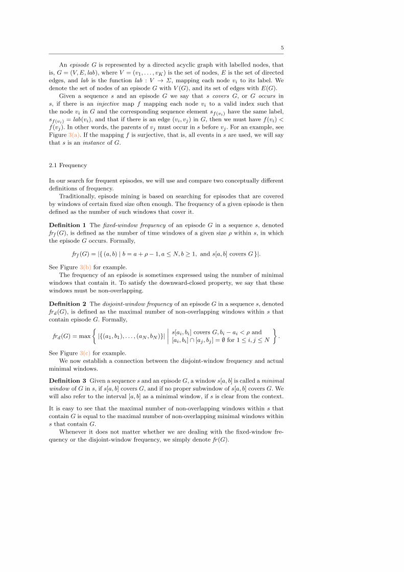
An episode G is represented by a directed acyclic graph with labelled nodes, that
is, G = (V,E, lab), where V = (v1, . . . , vK) is the set of nodes, E is the set of directed
edges, and lab is the function lab : V → Σ, mapping each node vi to its label. We
denote the set of nodes of an episode G with V (G), and its set of edges with E(G).
Given a sequence s and an episode G we say that s covers G, or G occurs in
s, if there is an injective map f mapping each node vi to a valid index such that
the node vi in G and the corresponding sequence element sf(vi) have the same label,
sf(vi) = lab(vi), and that if there is an edge (vi, vj) in G, then we must have f(vi) <
f(vj). In other words, the parents of vj must occur in s before vj . For an example, see
Figure 3(a)3(a). If the mapping f is surjective, that is, all events in s are used, we will say
that s is an instance of G.
2.1 Frequency
In our search for frequent episodes, we will use and compare two conceptually different
definitions of frequency.
Traditionally, episode mining is based on searching for episodes that are covered
by windows of certain fixed size often enough. The frequency of a given episode is then
defined as the number of such windows that cover it.
Definition 1 The fixed-window frequency of an episode G in a sequence s, denoted
frf (G), is defined as the number of time windows of a given size ρ within s, in which
the episode G occurs. Formally,
frf (G) = |{ (a, b) | b = a+ ρ− 1, a ≤ N, b ≥ 1, and s[a, b] covers G }|.
See Figure 3(b)3(b) for example.
The frequency of an episode is sometimes expressed using the number of minimal
windows that contain it. To satisfy the downward-closed property, we say that these
windows must be non-overlapping.
Definition 2 The disjoint-window frequency of an episode G in a sequence s, denoted
frd (G), is defined as the maximal number of non-overlapping windows within s that
contain episode G. Formally,
frd (G) = max
{|{(a1, b1), . . . , (aN , bN )}|
∣∣∣∣ s[ai, bi] covers G, bi − ai < ρ and
[ai, bi] ∩ [aj , bj ] = ∅ for 1 ≤ i, j ≤ N
}.
See Figure 3(c)3(c) for example.
We now establish a connection between the disjoint-window frequency and actual
minimal windows.
Definition 3 Given a sequence s and an episode G, a window s[a, b] is called a minimal
window of G in s, if s[a, b] covers G, and if no proper subwindow of s[a, b] covers G. We
will also refer to the interval [a, b] as a minimal window, if s is clear from the context.
It is easy to see that the maximal number of non-overlapping windows within s that
contain G is equal to the maximal number of non-overlapping minimal windows within
s that contain G.
Whenever it does not matter whether we are dealing with the fixed-window fre-
quency or the disjoint-window frequency, we simply denote fr(G).
6
a b
c d a c b a d b c d c a b d
(a) An example of an episode covered by a sequence
a b c a d c b d b a c d
(b) fixed-length windows
a b c a d c b d b a c d
(c) non-overlapping windows
Fig. 3 A toy example illustrating different support measures. Figure 3(a)3(a) contains an exampleof a sequence covering an episode. Figure 3(b)3(b) shows all 5 sliding windows of length 5 containingthe episode. Figure 3(c)3(c) shows the maximal number, 2, of non-overlapping windows coveringthe episode.
3 Strict Episodes
In this section we will define our mining problem and give a rough outline of the
discovery algorithm.
Generally, a pattern is considered closed if there exists no more specific pattern
having the same frequency. In order to speak of more specific patterns, we must first
have a way to describe episodes in these terms.
Definition 4 Assume two transitively closed episodes G and H with the same number
of nodes. An episode G is called a subepisode of episode H, denoted G � H if the set
of all sequences that cover H is a subset of the set of all sequences that cover G. If
the set of all sequences that cover H is a proper subset of the set of all sequences that
cover G, we call G a proper subepisode of H, denoted G ≺ H.
For a more general case, assume that |V (G)| < |V (H)|. We say that G is a
subepisode of H, denoted G � H, if there is a subgraph H ′ of H such that G � H ′.Moreover, let α be a graph homomorphism from H ′ to H. If we wish to emphasize α,
we write G �α H.
If |V (G)| > |V (H)|, then G is automatically not a subepisode of H.
The problem with this definition is that we do not have the means to compute this
relationship for general episodes. To do this, one would have to enumerate all possible
sequences that cover H and compute whether they cover G. We approach this problem
by restricting ourselves to a class of episodes where this comparison can be performed
efficiently.
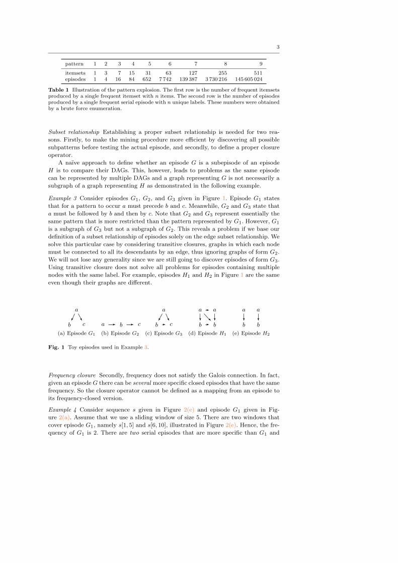
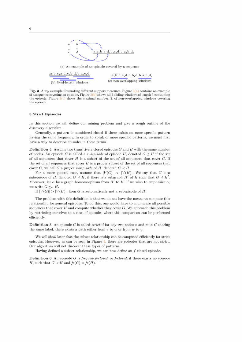
Definition 5 An episode G is called strict if for any two nodes v and w in G sharing
the same label, there exists a path either from v to w or from w to v.
We will show later that the subset relationship can be computed efficiently for strict
episodes. However, as can be seen in Figure 44, there are episodes that are not strict.
Our algorithm will not discover these types of patterns.
Having defined a subset relationship, we can now define an f -closed episode.
Definition 6 An episode G is frequency-closed, or f-closed, if there exists no episode
H, such that G ≺ H and fr(G) = fr(H).
7
a
c
a
b
(a) non-strict
a
c
a
b
(b) strict
Fig. 4 An example of a non-strict and a strict episode.
Problem 1 Given a sequence s, a frequency measure, either fixed-window or disjoint-
window, and a threshold σ, find all f -closed strict episodes from s having the frequency
higher or equal than σ.
A traditional approach to discovering closed patterns is to discover generators,
that is, for each closed pattern P , discover minimal patterns whose closure is equal to
P [1414]. When patterns are itemsets, it holds that the collection of frequent generators
are downward closed. Hence, they can be mined efficiently using a BFS-style approach.
We cannot directly apply this framework for two reasons: Firstly, unlike with item-
sets, we cannot define a closure based on frequency. We solve this by defining an
instance-closure, a more conservative closure that guarantees that all f -closed episodes
are discovered. Once instance-closed episodes are discovered, the f -closed episodes are
selected in a post-processing step. The second obstacle is the fact that the collection
of generator episodes is not necessarily downward-closed. We solve this problem by
additionally using some intermediate episodes that will guarantee the correctness of
the algorithm.
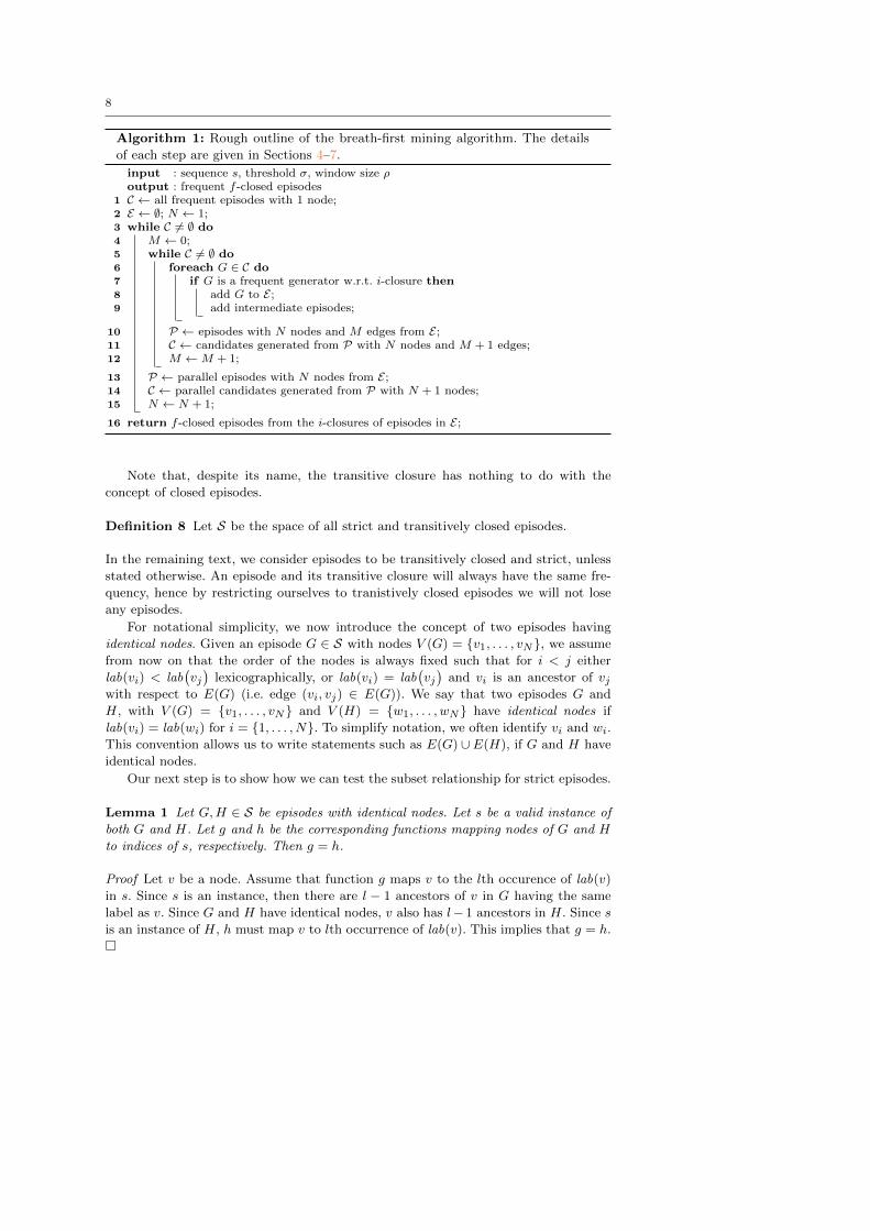
A sketch of the miner is given in Algorithm 11 (the details of the algorithm are
described in subsequent sections). The algorithm consists of two loops. In the outer
loop, Lines 33–1515, we discover parallel episodes by adding nodes. In the inner loop,
Lines 55–1212, we discover general episodes by adding edges. Each candidate episode is
tested, and if the candidate is frequent and a generator, then the episodes is added
into the collection. Finally, we discover the f -closed episodes as a last step.
To complete the algorithm we need to solve several subproblems:
1. computing the subset relationship efficiently (Section 44)
2. defining and computing instance-closure (Section 55)
3. generating candidate episodes, Line 1111 (Section 66)
4. generating intermediate episodes and proving the correctness (Section 77)
4 Computing The Subset Relationship
In this section we will demonstrate that computing the subset relationship for strict
episodes can be done efficiently. This allows us to build an algorithm to efficiently
discover closed episodes.
We now provide a canonical form for episodes, which will help us in further theorems
and algorithms. We define an episode that has the maximal number of edges using a
fundamental notion familiar from graph theory.
Definition 7 The transitive closure of an episode G = (V,E, lab) is an episode tcl(G),
where G and tcl(G) have the same set of nodes V , the same lab function mapping nodes
to labels, and the set of edges in tcl(G) is equal to
E(tcl(G)) = E ∪ { (vi, vj) | a path exists in G from vi to vj } .
8
Algorithm 1: Rough outline of the breath-first mining algorithm. The details
of each step are given in Sections 44–77.
input : sequence s, threshold σ, window size ρoutput : frequent f -closed episodes
1 C ← all frequent episodes with 1 node;2 E ← ∅; N ← 1;3 while C 6= ∅ do4 M ← 0;5 while C 6= ∅ do6 foreach G ∈ C do7 if G is a frequent generator w.r.t. i-closure then8 add G to E;9 add intermediate episodes;
10 P ← episodes with N nodes and M edges from E;11 C ← candidates generated from P with N nodes and M + 1 edges;12 M ←M + 1;
13 P ← parallel episodes with N nodes from E;14 C ← parallel candidates generated from P with N + 1 nodes;15 N ← N + 1;
16 return f -closed episodes from the i-closures of episodes in E;
Note that, despite its name, the transitive closure has nothing to do with the
concept of closed episodes.
Definition 8 Let S be the space of all strict and transitively closed episodes.
In the remaining text, we consider episodes to be transitively closed and strict, unless
stated otherwise. An episode and its transitive closure will always have the same fre-
quency, hence by restricting ourselves to tranistively closed episodes we will not lose
any episodes.
For notational simplicity, we now introduce the concept of two episodes having
identical nodes. Given an episode G ∈ S with nodes V (G) = {v1, . . . , vN}, we assume
from now on that the order of the nodes is always fixed such that for i < j either
lab(vi) < lab(vj)
lexicographically, or lab(vi) = lab(vj)
and vi is an ancestor of vjwith respect to E(G) (i.e. edge (vi, vj) ∈ E(G)). We say that two episodes G and
H, with V (G) = {v1, . . . , vN} and V (H) = {w1, . . . , wN} have identical nodes if
lab(vi) = lab(wi) for i = {1, . . . , N}. To simplify notation, we often identify vi and wi.
This convention allows us to write statements such as E(G) ∪E(H), if G and H have
identical nodes.
Our next step is to show how we can test the subset relationship for strict episodes.
Lemma 1 Let G,H ∈ S be episodes with identical nodes. Let s be a valid instance of
both G and H. Let g and h be the corresponding functions mapping nodes of G and H
to indices of s, respectively. Then g = h.
Proof Let v be a node. Assume that function g maps v to the lth occurence of lab(v)
in s. Since s is an instance, then there are l − 1 ancestors of v in G having the same
label as v. Since G and H have identical nodes, v also has l− 1 ancestors in H. Since s
is an instance of H, h must map v to lth occurrence of lab(v). This implies that g = h.
�
9
Lemma 11 implies that given an episode G and an instance s, there is only one
valid function f mapping nodes of G to indices of s. Let us denote this mapping by
map(G, s) = f . If G is a parallel episode with nodes V = V (G) we write map(V, s).
Crucially, we can easily compute the subset relationship between two episodes.
Theorem 1 For episodes G,H ∈ S with identical nodes, E(G) ⊆ E(H) if and only if
G � H.
Proof To prove the ”only if” direction assume that E(G) ⊆ E(H). Let s = {s1, . . . , sN}be an instance of H and let f = map(H, s) be the corresponding mapping. Then f is
also a valid mapping for G. Thus, G � H.
To prove the other direction, assume that E(G) * E(H). We therefore must have
an edge e = (x, y) ∈ E(G), such that e /∈ E(H). We build s by first visiting every
parent of y in H in a valid order with respect to H, then y itself, and then the rest
of the nodes, also in a valid order. Let h be the visiting order of G while constructing
s, that is, h(v) = 1, if we visited v first, h(v) = 2, if we visited v second. Note that
h(y) < h(x). Assume now that s covers G and let f = map(G, s) be the corresponding
mapping. But then Lemma 11 implies that g = h, thus g(y) < g(x), contradicting the
fact that (x, y) ∈ E(G). �
Theorem 11 essentially shows that our subset relationship is in fact a graph subset
relationship which allows us to design an efficient mining algorithm.
We finish this section by defining what we exactly mean when we say that two
episodes are equivalent and demonstrate that the class of strict episodes contains all
parallel episodes.
Definition 9 Episodes G and H are said to be equivalent, denoted by G ∼ H, if each
sequence that covers G also covers H, and vice versa.
Corollary 1 (of Theorem 11) For episodes G,H ∈ S, G ∼ H if and only if E(G) =
E(H) and G and H have identical nodes.
Proof This follows from the fact that G ∼ H is equivalent to G � H and H � G, and
that E(G) = E(H) is equivalent to E(G) ⊆ E(H) and E(H) ⊆ E(G). �
Note that by generating only transitively closed strict episodes, we have obtained an
efficient way of computing the subset relationship between two episodes. At first glance,
though, it may seem that we have completely omitted certain parallel episodes from
consideration — namely, all non-strict parallel episodes (i.e. those containing multiple
nodes with same labels). Note, however, that for each such episode G, there exists a
strict episode H, such that G ∼ H. To build such an episode H, we just need to create
edges that would strictly define the order among nodes with the same labels. From
now on, when we talk of parallel episodes, we actually refer to their strict equivalents.
5 Closure
Having defined a subset relationship among episodes, we are now able to speak of an
episode being more specific than another episode. However, this is only the first step
towards defining the closure of an episode. We know that the closure must be more
specific, but it must also be unique and well-defined. We have already seen that basing

10
such a closure on the frequency fails, as there can be multiple more specific closed
episodes that could be considered as closures.
In this section we will establish three closure operators, based on the instances of
the episode found within the sequence. The first closure adds nodes, the second one
adds edges, and the third is a combination of the first two. We also show that these
operators satisfy three important properties. We will use these properties to prove the
correctness of our mining algorithm. The needed properties for a closure operator h
are
1. Extension: G � h(G),
2. Idempotency: h(G) = h(h(G)),
3. Monotonicity: G1 � G2 ⇒ h(G1) � h(G2).
These properties are usually shown using the Galois connection but to avoid cum-
bersome notation we will prove them directly.
5.1 Node Closure
In this section we will define a node closure and show that it satisfies the properties.
Assume that we are given a sequence s and a window size ρ.
Our first step is to define a function fN which maps an episode G ∈ S to a set of
intervals which contain all instances of G,
fN (G; s) = { [minm,maxm] | sm covers G, maxm−minm < ρ,m ∈M } ,
where M contains all strictly increasing mappings to s.
Our next step is to define XG to be the set of all symbols occurring in each interval,
XG = {x ∈ Σ | x occurs in s[a, b] for all [a, b] ∈ fN (G) } .
Let W be the labels of the nodes of G. We define our first closure operator, iclN (G)
to be G augmented with nodes having the labels XG −W , that is, we add nodes to G
with labels that occur inside each window that contains G.
Theorem 2 iclN (G) is an idempotentic and monotonic extension operator.
Proof The extension property follows immediately because we are only adding new
nodes.
Assume now that G � H. Let [a, b] ∈ fN (H) be an interval. Then, there is an
interval [c, d] ∈ fN (G) such that a ≤ c ≤ d ≤ b. This means that any symbol occurring
in every interval in fN (G) will also occur in every interval in fN (H), that is, XG ⊆ XH .
Let α be a graph homomorphism such that G �α H. Let x ∈ XG be a symbol not
occurring in G and let v be the new node in iclN (G) with this label. If x does not occur
in H, then x ∈ XH and thus a node with a label x is added into H. In any case, there
is a node w with a label x in iclN (H). We can extend α by setting α(v) = w. By doing
this for each new node we have proved monotonicity, i.e. that iclN (G) � iclN (H).
To prove idempotency, let us write H = iclN (G). Since any new node in H must
occur inside the instances of G, we have fN (G) ⊆ fN (H). This implies that XH ⊆ XGand since we saw before that XG ⊆ XH , it implies that XG = XH . Since for every
label in XH there is a node in H with the same label, it holds that iclN (H) = H. �

11
Note that the node closure adds only events with unique labels. The reason for this
is that if we add node x to an episode containing node y such that lab(x) = lab(y),
then we would have to connect x and y. This may reduce the instances and invalidate
the proof. For the same reason, we only add a maximum of one new node with a
particular label. In other words, if each window containing episode G also contains two
occurrences of a, we will only add one node with label a to G (provided G does not
contain a node labelled a already).
5.2 Edge Closure
We begin by introducing the concept of a maximal episode that is covered by a given
set of sequences.
Definition 10 Given a set of nodes V , and a set S of instances of V, interpreted as
a parallel episode, we define the maximal episode covered by set S as the episode H,
where V (H) = V and
E(H) = { (x, y) ∈ V × V | f(x) < f(y), f = map(V, s) for all s ∈ S } ,
where map(V, s) refers to the mapping defined in Lemma 11 and V is interpreted as a
parallel episode.
To define a closure operator we first define a function mapping an episode G to all
of its valid instances in a sequence s,
fE(G; s) = { sm | sm covers G, maxm−minm < ρ,m ∈M } ,
where M contains all strictly increasing mappings to s. When the sequence is known
from the context, we denote simply fE(G)
We define iclE(G) to be the maximal episode covered by fE(G). If iclE(G) = G,
then we call G an e-closed episode.
Theorem 3 iclE(G) is an idempotentic and monotonic extension operator.
Proof To prove the extension property assume an edge (vi, vj) ∈ E(G). Let V be
the nodes in G. Let w ∈ fE(G) be an instance of G and let f = map(V,w) be the
corresponding mapping. Lemma 11 implies that map(V,w) = map(G,w). Hence f(vi) <
f(vj). Since this holds for every map, we have (vi, vj) ∈ E(iclE(G)).
To prove the idempotency, let H = iclE(G). The extension property implies that
G � H so by definition fE(H) ⊆ fE(G). But any instance in fE(G) also covers H.
Thus, fE(H) ⊆ fE(G) and so fE(H) = fE(G). This implies the idempotency.
Assume now that G � H. Let α be the graph homomorphism such that G �αH. We will show that iclE(G) �α iclE(H). Let (x, y) ∈ E(iclE(G)). Let w be an
instance of H and let f = map(H, s) the corresponding mapping to w. Assume that
f(α(x)) ≥ f(α(y)). Let v be the subsequence of w containing only the indices in the
range of f ◦ α. Note that v is a valid instance of G and f ◦ α = map(V (G), v). This
contradicts the fact that (x, y) ∈ E(iclE(G)). Hence, f(α(x)) < f(α(y)). This implies
that (α(x), α(y)) ∈ E(iclE(H)) which completes the proof. �
12
Example 5 Consider sequence s given in Figure 2(e)2(e) and episode G4 given in Fig-
ure 2(d)2(d) and assume that the window length is 5. There are four instances of G4 in
s, namely abcd, acdb, acbd and abcd. Therefore, fE(G4) = { abcd, acbd }. The serial
episodes corresponding to these subsequences are G2 and G3 given in Figure 22. By
taking the intersection of these two episodes we obtain G1 = iclE(G4) given in Fig-
ure 2(a)2(a).
5.3 Combining Closures
We can combine the node closure and the edge closure into one operator.
Definition 11 Given an episode G ∈ S, we define iclEN (G) = iclE(iclN (G)). To
simplify the notation, we will refer to iclEN (G) as icl(G), the i-closure of G. We will
say that G is i-closed if G = icl(G).
Theorem 4 icl(G) is an idempotentic and monotonic extension operator.
Proof The extension and monotonicity properties follow directly from the fact that
both iclN (G) and iclE(G) are monotonic extension operators.
To prove idempotency let H = icl(G) and H ′ = iclN (G). Since any instance of
H = iclE(H ′) is also an instance of H ′, and, per definition, vice versa, we see that
fN (H) = fN (H ′), and consequently iclN (H) = H, and icl(H) = iclE(iclN (H)) =
iclE(H) = H. �
The advantage of mining i-closed episodes instead of e-closed is prominent if the
sequence contains a long sequential pattern. More specifically, assume that the input
sequence contains a frequent subsequence of N symbols p1, . . . , pN , and no other per-
mutation of this pattern occurs in the sequence. The number of e-closed subpatterns
of this subsequence is 2N − 1, namely, all non-empty serial subepisodes. However,
the number of its i-closed subpatterns is N(N + 1)/2, namely, serial episodes of form
pi → · · · → pj for 1 ≤ i ≤ j ≤ N .
5.4 Computing Closures
During the mining process, we need to compute the closure of an episode. The definition
of closures use fN (G) and fE(G) which are based on instances of G in s. However,
there can be an exponential number of such instances in s.
In the following discussion we will often use the following notations. Given an
episode G, we write G+ v to mean the episode G augmented with an additional node
v. Similarly, we will use the notations G + e and G + V , where e is an edge and V is
a set of nodes. We also use G − v, G − V , and G − e to mean episodes where either
nodes or edges are removed.
To avoid the problem of an exponential number of instances we make two observa-
tions: Firstly, a node with a new label l is added into the closure if and only if it occurs
in every minimal window of G. Secondly, an edge (x, y) is added into the closure if
and only if there is no minimal window for G + (y, x). Thus to compute the closure
we need an algorithm that finds all minimal windows of G in s. Note that, unlike with
instances of G, there can be only |s| minimal windows.
Using strict episodes allows us to discover minimal windows in an efficient greedy
fashion.
13
Lemma 2 Given an episode G ∈ S and a sequence s = s1 · · · sL, let k be the smallest
index such that sk = lab(v), where v is a source node in G. Then s covers G if and
only if s[k + 1, L] covers G− v.
Proof Let f be a mapping from V (G) to s. If k is not already used by f , then we can
remap a source node v to k. As k is the smallest entry used by f , the remaining map
is a valid mapping for G− v in s[k + 1, L]. �
Lemma 22 says that to test whether a sequence s covers G, it is sufficient to greedily
find entries from s corresponding to the sources of G, removing those sources as we
move along. Let us denote such a mapping by g(G; s). Note that if the episode is not
strict, then we can have two source nodes with the same label, in which case it might be
that Lemma 22 holds for one of the sources but not for the other. Since we cannot know
in advance which node to choose, this ambiguity would make the greedy approach less
efficient.
Lemma 3 Let G ∈ S be an episode and let s be a sequence covering G. Let m = g(G; s)
and let [a, b] be the first minimal window of G in s. Then maxm = b.
Proof Since s[1, b] covers G, there is a mapping m′ = g(G; s[1, b]). Since [a, b] is the
first minimal window, we must have maxm′ = b. Since m and m′ are constructed in a
greedy fashion, we must have m = m′. �
Lemma 33 states that if we evaluate m = g(G; s[k, L]) for each k = 1, . . . ,K, store
the intervals W = [minm,maxm], and for each pair of windows [a1, b], [a2, b] ∈ W
remove [a2, b], then W will contain the minimal windows. Evaluating g(G; s) can be
done in polynomial time, so this approach takes polynomial time. The algorithm for
discovering minimal windows is given in Algorithm 22. To fully describe the algorithm
we need the following definition.
Definition 12 An edge (v, w) in an episode G ∈ S is called a skeleton edge if there is
no node u such that (v, u, w) is a path in G. If v and w have different labels, we call
the edge (v, w) a proper skeleton edge.
Theorem 5 Algorithm FindWindows discovers all minimal windows.
Proof We will prove the correctness of the algorithm in several steps. First, we will
show that the loop 88–1616 guarantees that f is truly a valid mapping. To see this, note
that the loop upholds the following invariants: For every v /∈ Q, we have f(v) > b(v)
and for each skeleton edge (v, w), we have b(w) 6= −∞. Also, for every non-source node
w, b(w) = max { f(v) | (v, w) is a skeleton edge } or b(w) = −∞.
Thus when we leave the loop, that is, Q = ∅, then f is a valid mapping for G.
Moreover, since we select the smallest f(v) during Line 1111, we can show using recursion
that f = g(G; s[k + 1, L]), where k = min b(v), where the min ranges over all source
nodes. Once f is discovered, the next new mapping should be contained in s[min f +
1, L]. This is exactly what is done on Line 2222 by making b(v) equal to f(v). �
The advantage of this approach is that we can now optimize the search on Line 1111
by starting the search from the previous index f(v) instead of starting from the start
of the sequence. The following lemma, implied directly by the greedy procedure, allows
this.

14
Algorithm 2: FindWindows. An algorithm for finding minimal windows of G
from s. The parameter ρ is the maximal size of the window.
input : an episode G ∈ Sinput : set of minimal windows W
1 W ← ∅;2 Q← ∅;3 foreach v ∈ V (G) do4 f(v)← first i such that si = lab(v);5 b(v)← −∞;6 add v into Q;
7 while true do{Make sure that f honors the edges in G}
8 while Q is not empty do9 v ← first element in Q;
10 remove v from Q;11 f(v)← the smallest i > b(v) such that si = lab(v);12 if f(v) = null then return W ;13 foreach skeleton edge (v, w) ∈ E(G) do14 b(w)← max(b(w), f(v));15 if b(w) ≥ f(w) and w /∈ Q then16 add w into Q;
17 if max f −min f < ρ then18 if max f = b such that [a, b] is the last entry in W then19 delete the last entry from W ;
20 add [min f,max f ] to W ;
21 v ← node with the smallest f(v);22 b(v)← f(v);23 add v to Q;
Lemma 4 Let G ∈ S be an episode and let s be a sequence covering G. Let k be an
index and assume that s[k, L] covers G. Set m1 = g(G; s) and m2 = g(G; s[k + 1, L]).
Then m2(v) ≥ m1(v) for every v ∈ V (G).
Let us now analyze the complexity of FindWindows. Assume that the input
episode G has N nodes and the input sequence s has L symbols. Let K be the max-
imal number of nodes in G sharing the same label. Let D be the maximal number of
outgoing skeleton edges in a single node. Note that each event in s is visited during
Line 1111 K times, at maximum. Each visit may require D updates of b(w), at max-
imum. The only remaining non-trivial step is finding the minimal source (Line 2121),
which can be done with a heap in O(logN) time. This brings the total evaluation
time to O((D + 1)KL+ L logN). Note that for parallel episodes D = 0 and for serial
episodes D = 1, and for such episodes we can further optimize the algorithm such that
each event is visited only twice, thus making the running time to be in O(L logN) for
parallel episodes and in O(L) for serial episodes. Since there can be only L minimal
windows, the additional space complexity for the algorithm is in O(L).
Given the set of minimal windows, we can now compute the node closure by testing
which nodes occur in all minimal windows. This can be done in O(L) time. To compute
the edge closure we need to perform N2 calls of FindWindows. This can be greatly
optimized by sieving multiple edges simultaneously based on valid mappings f dis-
covered during FindWindows. In addition, we can compute both frequency measures
from minimal windows in O(L) time.
15
We will now turn to discovering f -closed episodes. Note that, unlike the i-closure,
we do not define an f -closure of an episode at all. As shown in Section 11, such an
f -closure would not necessarily be unique. However, the set of i-closed episodes will
contain all f -closed episodes.
Theorem 6 An f-closed episode is always i-closed.
Proof Let G ∈ S be an episode and define H = icl(G). Let W be a set of all minimal
windows of s that cover G and let V be the set of all minimal windows that cover H.
Let w = [a, b] ∈ W be a minimal window of G and let f be a valid mapping from G
to s[a, b]. Any new node added in H must occur in s[a, b] and f can be extended to H
such that it honours all edges in H. Hence s[a, b] covers H. It is also a minimal window
for H because otherwise it would violate the minimality for G. Hence w ∈ V . Now
assume that v = [a′, b′] ∈ V . Obviously, s[a′, b′] covers G, so there must be a minimal
window w = [a, b] ∈W . Using the first argument we see that w ∈ V . Since V contains
only minimal windows we conclude that v = w. Hence W = V . A sequence covers an
episode if and only if the sequence contains a minimal window of the episode. Thus,
by definition, V = W implies that frf (G) = frf (H) and frd (G) = frd (H).
Assume now that G is not i-closed, then G 6= H, and since fr(G) = fr(H), G is not
f -closed either. This completes the proof. �
A naıve approach to extract f -closed episodes would be to compare each pair of
instance-closed episodes G and H and if fr(G) = fr(H) and G ≺ H, remove G from
the output. This approach can be considerably sped up by realising that we need
only to test episodes with identical nodes and episodes of form G − V , where V is a
subset of V (G). The pseudo-code is given in Algorithm 33. The algorithm can be further
sped up by exploiting the subset relationship between the episodes. Our experiments
demonstrate that this comparison is feasible in practice.
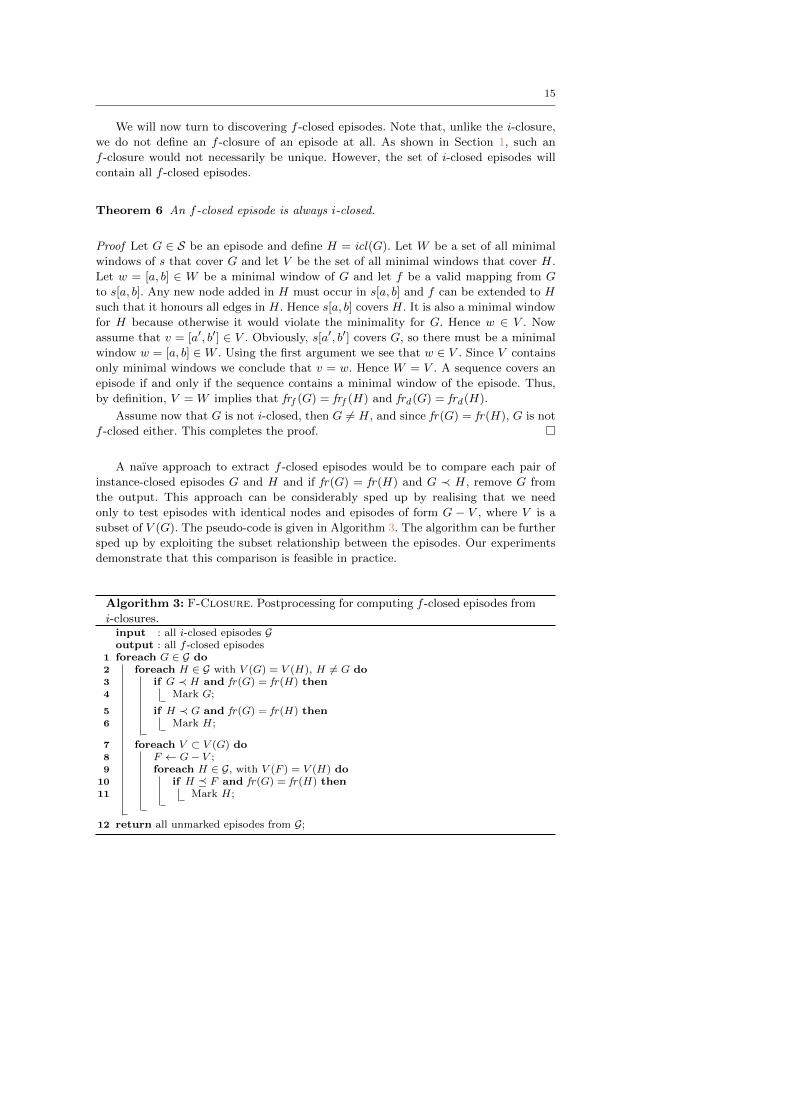
Algorithm 3: F-Closure. Postprocessing for computing f -closed episodes from
i-closures.input : all i-closed episodes Goutput : all f -closed episodes
1 foreach G ∈ G do2 foreach H ∈ G with V (G) = V (H), H 6= G do3 if G ≺ H and fr(G) = fr(H) then4 Mark G;
5 if H ≺ G and fr(G) = fr(H) then6 Mark H;
7 foreach V ⊂ V (G) do8 F ← G− V ;9 foreach H ∈ G, with V (F ) = V (H) do
10 if H � F and fr(G) = fr(H) then11 Mark H;
12 return all unmarked episodes from G;
16
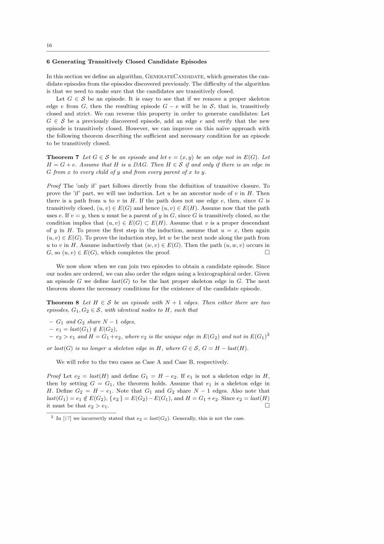
6 Generating Transitively Closed Candidate Episodes
In this section we define an algorithm, GenerateCandidate, which generates the can-
didate episodes from the episodes discovered previously. The difficulty of the algorithm
is that we need to make sure that the candidates are transitively closed.
Let G ∈ S be an episode. It is easy to see that if we remove a proper skeleton
edge e from G, then the resulting episode G − e will be in S, that is, transitively
closed and strict. We can reverse this property in order to generate candidates: Let
G ∈ S be a previously discovered episode, add an edge e and verify that the new
episode is transitively closed. However, we can improve on this naıve approach with
the following theorem describing the sufficient and necessary condition for an episode
to be transitively closed.
Theorem 7 Let G ∈ S be an episode and let e = (x, y) be an edge not in E(G). Let
H = G + e. Assume that H is a DAG. Then H ∈ S if and only if there is an edge in
G from x to every child of y and from every parent of x to y.
Proof The ’only if’ part follows directly from the definition of transitive closure. To
prove the ’if’ part, we will use induction. Let u be an ancestor node of v in H. Then
there is a path from u to v in H. If the path does not use edge e, then, since G is
transitively closed, (u, v) ∈ E(G) and hence (u, v) ∈ E(H). Assume now that the path
uses e. If v = y, then u must be a parent of y in G, since G is transitively closed, so the
condition implies that (u, v) ∈ E(G) ⊂ E(H). Assume that v is a proper descendant
of y in H. To prove the first step in the induction, assume that u = x, then again
(u, v) ∈ E(G). To prove the induction step, let w be the next node along the path from
u to v in H. Assume inductively that (w, v) ∈ E(G). Then the path (u,w, v) occurs in
G, so (u, v) ∈ E(G), which completes the proof. �
We now show when we can join two episodes to obtain a candidate episode. Since
our nodes are ordered, we can also order the edges using a lexicographical order. Given
an episode G we define last(G) to be the last proper skeleton edge in G. The next
theorem shows the necessary conditions for the existence of the candidate episode.
Theorem 8 Let H ∈ S be an episode with N + 1 edges. Then either there are two
episodes, G1, G2 ∈ S, with identical nodes to H, such that
– G1 and G2 share N − 1 edges,
– e1 = last(G1) /∈ E(G2),
– e2 > e1 and H = G1 +e2, where e2 is the unique edge in E(G2) and not in E(G1)3
or last(G) is no longer a skeleton edge in H, where G ∈ S, G = H − last(H).
We will refer to the two cases as Case A and Case B, respectively.
Proof Let e2 = last(H) and define G1 = H − e2. If e1 is not a skeleton edge in H,
then by setting G = G1, the theorem holds. Assume that e1 is a skeleton edge in
H. Define G2 = H − e1. Note that G1 and G2 share N − 1 edges. Also note that
last(G1) = e1 /∈ E(G2), { e2 } = E(G2)−E(G1), and H = G1 +e2. Since e2 = last(H)
it must be that e2 > e1. �
3 In [1717] we incorrectly stated that e2 = last(G2). Generally, this is not the case.

17
Theorem 88 gives us means to generate episodes. Let us first consider Case A in
Theorem 88. To generate H we simply find all pairs of episodes G1 and G2 such that
the conditions of Case A in Theorem 88 hold. When combining G1 and G2 we need to
test whether the resulting episode is transitively closed.
Theorem 9 Let G1, G2 ∈ S be two episodes with identical nodes and N edges. Assume
that G1 and G2 share N − 1 mutual edges. Let e1 = (x1, y1) ∈ E(G1)− E(G2) be the
unique edge of G1 and let e2 = (x2, y2) ∈ E(G2) − E(G1) be the unique edge of G2.
Let H = G1 + e2. Assume that H has no cycles. Then H ∈ S if and only if one of the
following conditions is true:
1. x1 6= y2 and x2 6= y1.
2. x1 6= y2, x2 = y1, and (x1, y2) is an edge in G1.
3. x1 = y2, x2 6= y1, and (x2, y1) is an edge in G1.
Moreover, if H ∈ S, then e1 and e2 are both skeleton edges in H.
Proof We will first show that e1 is a skeleton edge in H if H ∈ S. If it is not, then
there is a path from x1 to y1 in H not using e1. The edges along this path also occur in
G2, thus forcing e1 to be an edge in G2, which is a contradiction. A similar argument
holds for e2.
The ”only if” part is trivial so we only prove the ”if” part using Theorem 77.
Let v be a child of y2 in G1 and f = (y2, v) an edge in G1.
If the first or second condition holds, then x1 6= y2, and consequently f 6= e1,
so f ∈ G2. The path (x2, y2, v) connects x2 and v in G2 so there must be an edge
h = (x2, v) in G2. Since h 6= e2, h must also occur in G1. If the third condition holds,
it may be the case that f = e1 (if not, then we can use the previous argument). But
in such a case v = y1 and edge h = (x2, y1) occurs in G1.
If now u is a parent of x2 in G1, we can make a similar argument that u and y2are connected, so Theorem 77 now implies that H is transitively closed. �
Theorem 99 allows us to handle Case A of Theorem 88. To handle Case B, we simply
take an episode G and try to find all edges e2 such that last(G+ e2) = e2 and last(G)
is no longer a skeleton edge in G + e2. The conditions for this are given in the next
theorem.
Theorem 10 Let G ∈ S be an episode, let e1 = (x1, y1) be a skeleton edge of G, and
let e2 = (x2, y2) be an edge not occurring in G and define H = G+ e2. Assume H ∈ Sand that e1 is not a skeleton edge in H. Then either y2 = y1 and (x1, x2) is a skeleton
edge in G or x1 = x2 and (y2, y1) is a skeleton edge in G.
Proof Assume that e1 is no longer a skeleton edge in H, then there is a path of skeleton
edges going from x1 to y1 in H not using e1. The path must use e2, otherwise we have a
contradiction. The theorem will follow if we can show that the path must have exactly
two edges. Assume otherwise. Assume, for simplicity, that edge e2 does not occur first
in the path and let z be the node before x2 in the path. Then we can build a new
path by replacing edges (z, x2) and e2 with (z, y2). This path does not use e2, hence
it occurs in G. If z 6= x1 or y1 6= y2, then the path makes e1 a non-skeleton edge in G,
which is a contradiction. If e2 is the first edge in the path, we can select the next node
after y2 and repeat the argument. �
18
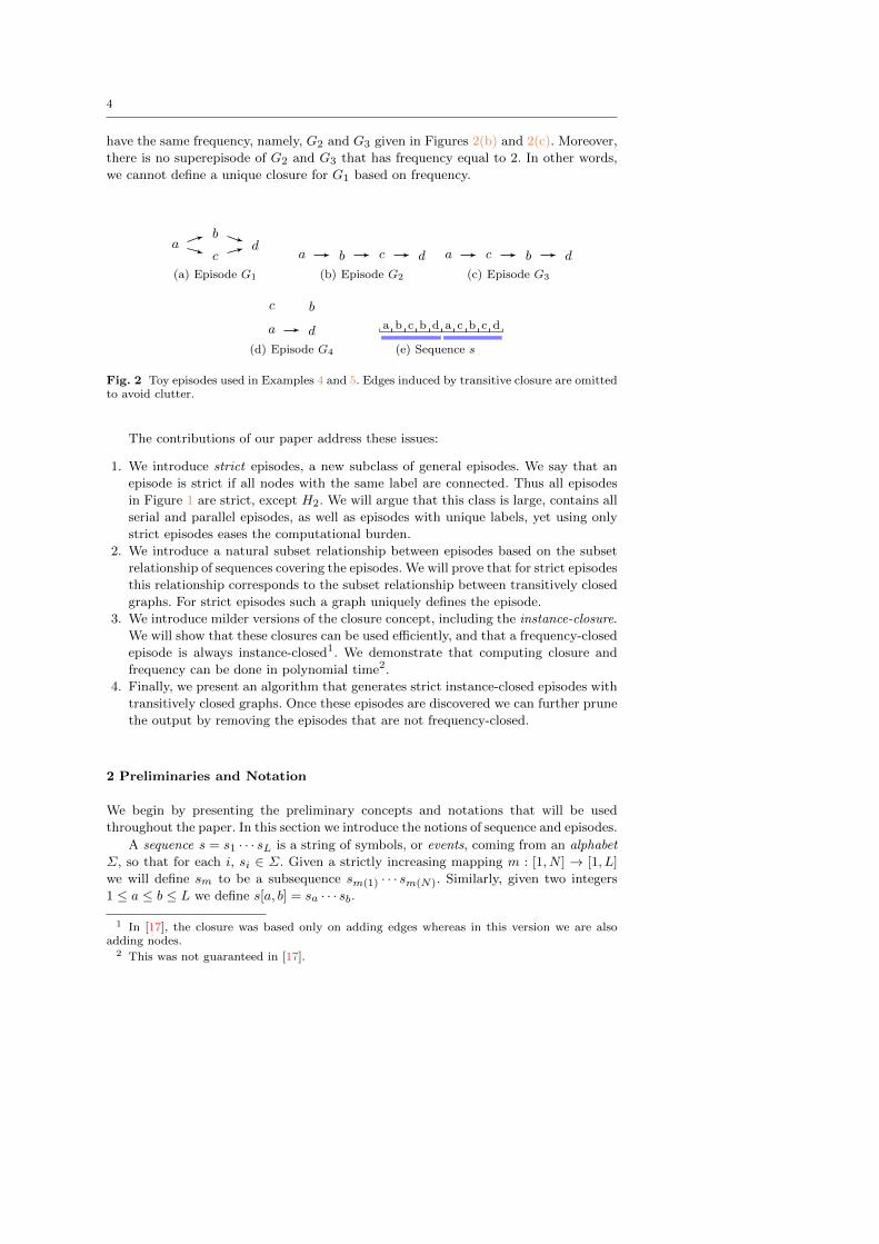
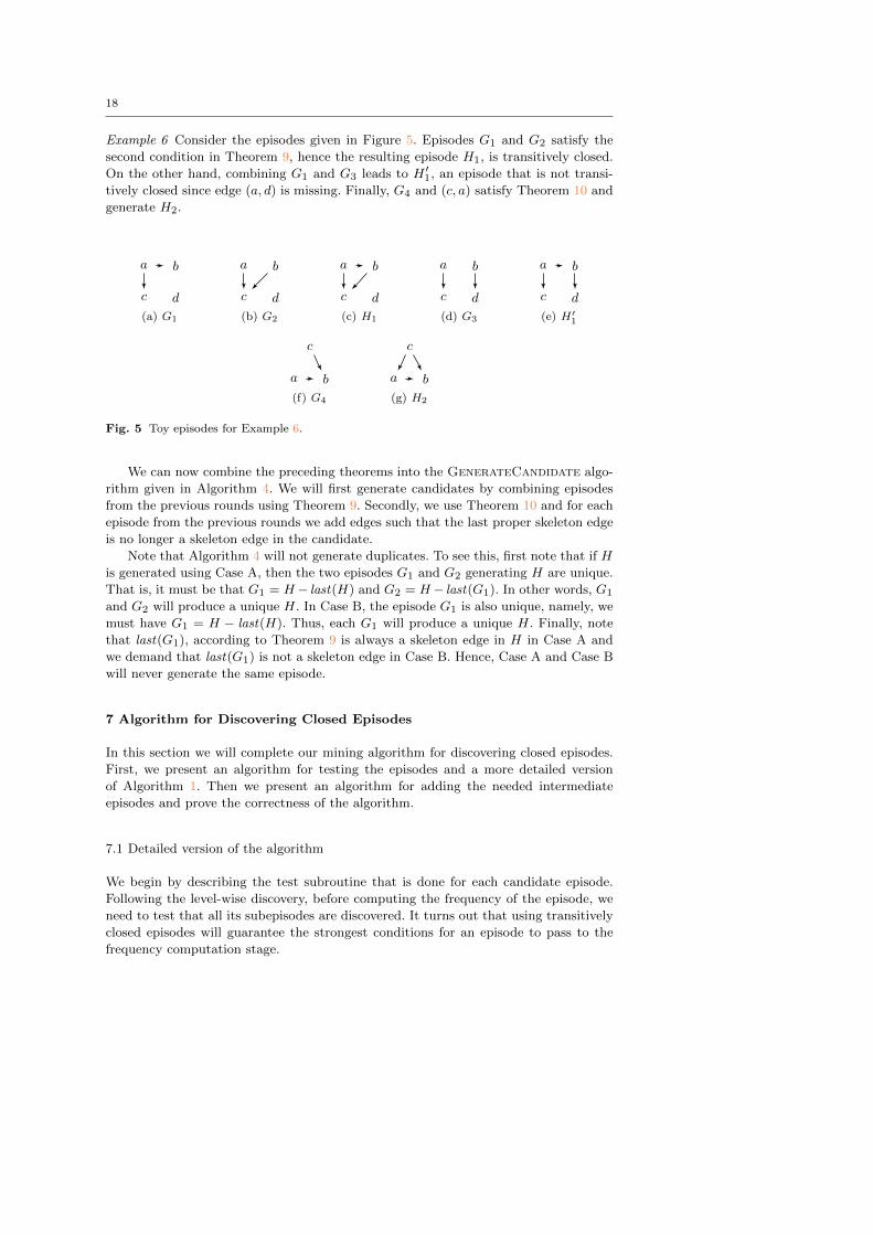
Example 6 Consider the episodes given in Figure 55. Episodes G1 and G2 satisfy the
second condition in Theorem 99, hence the resulting episode H1, is transitively closed.
On the other hand, combining G1 and G3 leads to H ′1, an episode that is not transi-
tively closed since edge (a, d) is missing. Finally, G4 and (c, a) satisfy Theorem 1010 and
generate H2.
a
c
b
d
(a) G1
a
c
b
d
(b) G2
a
c
b
d
(c) H1
a
c
b
d
(d) G3
a
c
b
d
(e) H′1
a
c
b
(f) G4
a
c
b
(g) H2
Fig. 5 Toy episodes for Example 66.
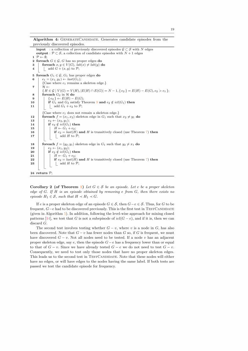
We can now combine the preceding theorems into the GenerateCandidate algo-
rithm given in Algorithm 44. We will first generate candidates by combining episodes
from the previous rounds using Theorem 99. Secondly, we use Theorem 1010 and for each
episode from the previous rounds we add edges such that the last proper skeleton edge
is no longer a skeleton edge in the candidate.
Note that Algorithm 44 will not generate duplicates. To see this, first note that if H
is generated using Case A, then the two episodes G1 and G2 generating H are unique.
That is, it must be that G1 = H− last(H) and G2 = H− last(G1). In other words, G1
and G2 will produce a unique H. In Case B, the episode G1 is also unique, namely, we
must have G1 = H − last(H). Thus, each G1 will produce a unique H. Finally, note
that last(G1), according to Theorem 99 is always a skeleton edge in H in Case A and
we demand that last(G1) is not a skeleton edge in Case B. Hence, Case A and Case B
will never generate the same episode.
7 Algorithm for Discovering Closed Episodes
In this section we will complete our mining algorithm for discovering closed episodes.
First, we present an algorithm for testing the episodes and a more detailed version
of Algorithm 11. Then we present an algorithm for adding the needed intermediate
episodes and prove the correctness of the algorithm.
7.1 Detailed version of the algorithm
We begin by describing the test subroutine that is done for each candidate episode.
Following the level-wise discovery, before computing the frequency of the episode, we
need to test that all its subepisodes are discovered. It turns out that using transitively
closed episodes will guarantee the strongest conditions for an episode to pass to the
frequency computation stage.
19
Algorithm 4: GenerateCandidate. Generates candidate episodes from the
previously discovered episodes.
input : a collection of previously discovered episodes G ⊂ S with N edgesoutput : P ⊂ S, a collection of candidate episodes with N + 1 edges
1 P ← ∅;2 foreach G ∈ G, G has no proper edges do3 foreach x, y ∈ V (G), lab(x) 6= lab(y) do4 add G+ (x, y) to P;
5 foreach G1 ∈ G, G1 has proper edges do6 e1 = (x1, y1)← last(G1);
{Case where e1 remains a skeleton edge.}7 H ←
{H ∈ G | V (G) = V (H), |E(H) ∩ E(G)| = N − 1, { e2 } = E(H)− E(G), e2 > e1 };8 foreach G2 in H do9 { e2 } ← E(H)− E(G);
10 if G1 and G2 satisfy Theorem 99 and e2 /∈ icl(G1) then11 add G1 + e2 to P;
{Case where e1 does not remain a skeleton edge.}12 foreach f = (x1, x2) skeleton edge in G1 such that x2 6= y1 do13 e2 ← (x2, y1);14 if e2 /∈ icl(G1) then15 H ← G1 + e2;16 if e2 = last(H) and H is transitively closed (use Theorem 77) then17 add H to P;
18 foreach f = (y2, y1) skeleton edge in G1 such that y2 6= x1 do19 e2 ← (x1, y2);20 if e2 /∈ icl(G1) then21 H ← G1 + e2;22 if e2 = last(H) and H is transitively closed (use Theorem 77) then23 add H to P;
24 return P;
Corollary 2 (of Theorem 11) Let G ∈ S be an episode. Let e be a proper skeleton
edge of G. If H is an episode obtained by removing e from G, then there exists no
episode H1 ∈ S, such that H ≺ H1 ≺ G.
If e is a proper skeleton edge of an episode G ∈ S, then G−e ∈ S. Thus, for G to be
frequent, G−e had to be discovered previously. This is the first test in TestCandidate
(given in Algorithm 55). In addition, following the level-wise approach for mining closed
patterns [1414], we test that G is not a subepisode of icl(G− e), and if it is, then we can
discard G.
The second test involves testing whether G − v, where v is a node in G, has also
been discovered. Note that G− v has fewer nodes than G so, if G is frequent, we must
have discovered G − v. Not all nodes need to be tested. If a node v has an adjacent
proper skeleton edge, say e, then the episode G−e has a frequency lower than or equal
to that of G − v. Since we have already tested G − e we do not need to test G − v.
Consequently, we need to test only those nodes that have no proper skeleton edges.
This leads us to the second test in TestCandidate. Note that these nodes will either
have no edges, or will have edges to the nodes having the same label. If both tests are
passed we test the candidate episode for frequency.

20
Example 7 Consider the episodes given in Figure 66. When testing the candidate episode
H, TestCandidate will test for the existence of three episodes. Episodes G1 and G2
are tested when either edge is removed and G3 is tested when node labelled d is
removed.
a
cb
d
(a) H
a
cb
d
(b) G1
a
cb
d
(c) G2
a
cb
(d) G3
Fig. 6 Toy episodes for Example 77.
Algorithm 5: TestCandidate. An algorithm that checks if an episode is a
proper candidate.
input : an episode G ∈ S, already discovered episodes C ⊂ Soutput : a boolean value, true only if all subepisodes of G are frequent
1 foreach proper skeleton edge e in G do2 if G− e /∈ C or e ∈ E(icl(G− e)) then3 return false;
4 foreach v in G not having a proper skeleton edge do5 if G− v /∈ C then6 return false;
7 if v has no edges and there is a node w ∈ V (icl(G− v)) s.t. lab(w) = lab(v) then8 return false;
9 return true;
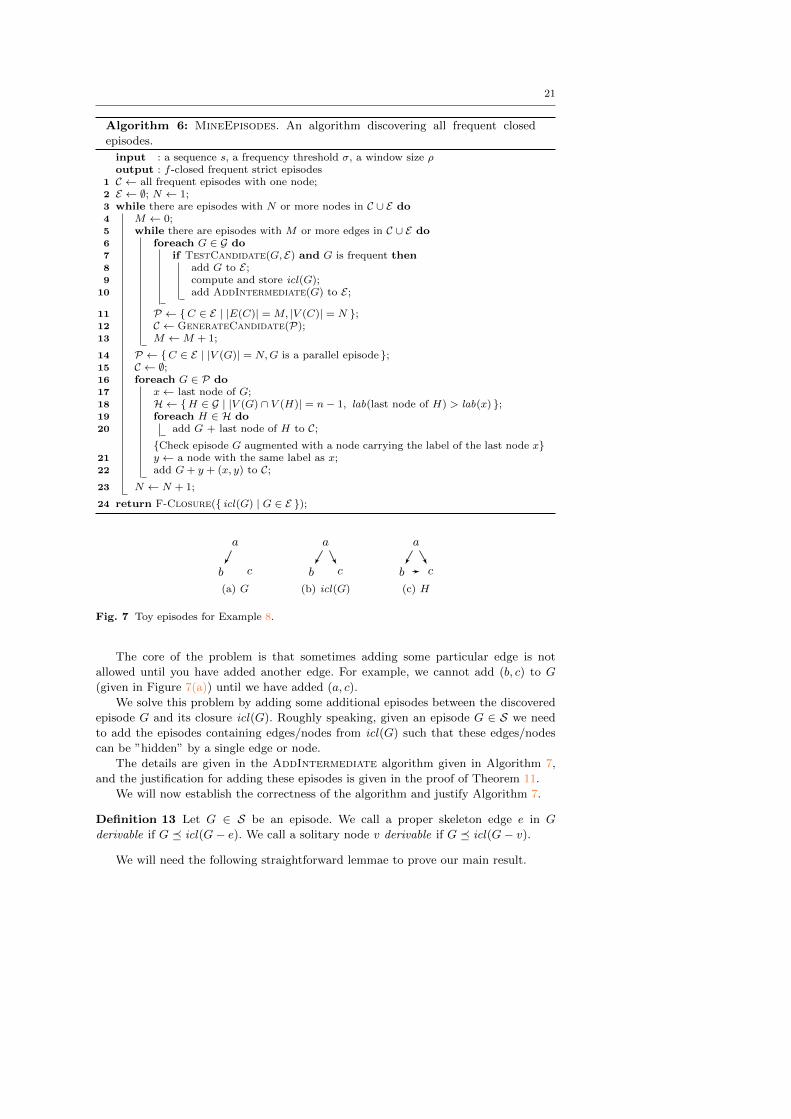
Finally we present a more detailed version of Algorithm 11, given in Algorithm 66.
The only missing part of the algorithm is the AddIntermediate subroutine which we
will give in the next section along with the proof of correctness.
7.2 Proof of Correctness
In the original framework for mining itemsets, the algorithm discovers itemset gen-
erators, the smallest itemsets that produce the same closure. It can be shown that
generators form a downward closed collection, so they can be discovered efficiently.
This, however, is not true for episodes, as the following example demonstrates.
Example 8 Consider the episodes given in Figure 77 and a sequence s = acbxxabcxxbac.
Assume that the window size is ρ = 3 and the frequency threshold is σ = 1. The
frequency of H is 1 and there is no subepisode that has the same frequency. Hence
to discover this episode all of its maximal subepisodes need to be discovered. One
of these subepisodes is icl(G). However, icl(G) is not added into E since (a, c) ∈icl(icl(G)− (a, c)) and TestCandidate returns false.
21
Algorithm 6: MineEpisodes. An algorithm discovering all frequent closed
episodes.
input : a sequence s, a frequency threshold σ, a window size ρoutput : f -closed frequent strict episodes
1 C ← all frequent episodes with one node;2 E ← ∅; N ← 1;3 while there are episodes with N or more nodes in C ∪ E do4 M ← 0;5 while there are episodes with M or more edges in C ∪ E do6 foreach G ∈ G do7 if TestCandidate(G, E) and G is frequent then8 add G to E;9 compute and store icl(G);
10 add AddIntermediate(G) to E;
11 P ← {C ∈ E | |E(C)| = M, |V (C)| = N };12 C ← GenerateCandidate(P);13 M ←M + 1;
14 P ← {C ∈ E | |V (G)| = N,G is a parallel episode };15 C ← ∅;16 foreach G ∈ P do17 x← last node of G;18 H ← {H ∈ G | |V (G) ∩ V (H)| = n− 1, lab(last node of H) > lab(x) };19 foreach H ∈ H do20 add G + last node of H to C;
{Check episode G augmented with a node carrying the label of the last node x}21 y ← a node with the same label as x;22 add G+ y + (x, y) to C;23 N ← N + 1;
24 return F-Closure({ icl(G) | G ∈ E });
a
cb
(a) G
a
cb
(b) icl(G)
a
cb
(c) H
Fig. 7 Toy episodes for Example 88.
The core of the problem is that sometimes adding some particular edge is not
allowed until you have added another edge. For example, we cannot add (b, c) to G
(given in Figure 7(a)7(a)) until we have added (a, c).
We solve this problem by adding some additional episodes between the discovered
episode G and its closure icl(G). Roughly speaking, given an episode G ∈ S we need
to add the episodes containing edges/nodes from icl(G) such that these edges/nodes
can be ”hidden” by a single edge or node.
The details are given in the AddIntermediate algorithm given in Algorithm 77,
and the justification for adding these episodes is given in the proof of Theorem 1111.
We will now establish the correctness of the algorithm and justify Algorithm 77.
Definition 13 Let G ∈ S be an episode. We call a proper skeleton edge e in G
derivable if G � icl(G− e). We call a solitary node v derivable if G � icl(G− v).
We will need the following straightforward lemmae to prove our main result.
22
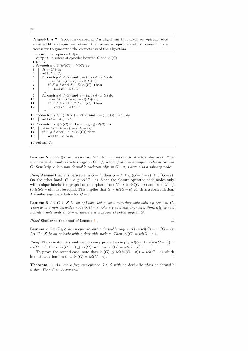
Algorithm 7: AddIntermediate. An algorithm that given an episode adds
some additional episodes between the discovered episode and its closure. This is
necessary to guarantee the correctness of the algorithm.
input : an episode G ∈ Soutput : a subset of episodes between G and icl(G)
1 C ← ∅;2 foreach x ∈ V (icl(G))− V (G) do3 H ← G+ x;4 add H to C;5 foreach y ∈ V (G) and e = (x, y) /∈ icl(G) do6 Z ← E(tcl(H + e))− E(H + e);7 if Z 6= ∅ and Z ⊂ E(icl(H)) then8 add H + Z to C;
9 foreach y ∈ V (G) and e = (y, x) /∈ icl(G) do10 Z ← E(tcl(H + e))− E(H + e);11 if Z 6= ∅ and Z ⊂ E(icl(H)) then12 add H + Z to C;
13 foreach x, y ∈ V (icl(G))− V (G) and e = (x, y) /∈ icl(G) do14 add G+ x+ y to C;15 foreach x, y ∈ V (G) and e = (x, y) /∈ icl(G) do16 Z ← E(tcl(G+ e))− E(G+ e);17 if Z 6= ∅ and Z ⊂ E(icl(G)) then18 add G+ Z to C;
19 return C;
Lemma 5 Let G ∈ S be an episode. Let e be a non-derivable skeleton edge in G. Then
e is a non-derivable skeleton edge in G − f , where f 6= e is a proper skeleton edge in
G. Similarly, e is a non-derivable skeleton edge in G− v, where v is a solitary node.
Proof Assume that e is derivable in G− f , then G− f � icl(G− f − e) � icl(G− e).On the other hand, G − e � icl(G− e). Since the closure operator adds nodes only
with unique labels, the graph homomorpisms from G− e to icl(G− e) and from G− fto icl(G− e) must be equal. This implies that G � icl(G− e) which is a contradiction.
A similar argument holds for G− v. �
Lemma 6 Let G ∈ S be an episode. Let w be a non-derivable solitary node in G.
Then w is a non-derivable node in G− v, where v is a solitary node. Similarly, w is a
non-derivable node in G− e, where e is a proper skeleton edge in G.
Proof Similar to the proof of Lemma 55. �
Lemma 7 Let G ∈ S be an episode with a derivable edge e. Then icl(G) = icl(G− e).
Let G ∈ S be an episode with a derivable node v. Then icl(G) = icl(G− v).
Proof The monotonicity and idempotency properties imply icl(G) � icl(icl(G− e)) =
icl(G− e). Since icl(G− e) � icl(G), we have icl(G) = icl(G− e).To prove the second case, note that icl(G) � icl(icl(G− v)) = icl(G− v) which
immediately implies that icl(G) = icl(G− v). �
Theorem 11 Assume a frequent episode G ∈ S with no derivable edges or derivable
nodes. Then G is discovered.
23
Proof We will prove the theorem by induction. Obviously, the theorem holds for episodes
with a single node. Assume now that the theorem is true for all subepisodes of G.
Episode G will be discovered if it passes the tests in TestCandidate. To pass these
tests, all episodes of form G−e, where e is a proper skeleton edge need to be discovered.
Assume that all these subepisodes are discovered but we have e ∈ E(icl(G− e)). This
means, by definition, that e is a derivable edge in G which is a contradiction. The same
argument holds for episodes of form G− v, where v is a node.
Now assume that one of the subepisodes, say, H is not discovered. The induction
assumption now implies that H has either derivable nodes or edges.
Lemma 8 There is a subepisode F ∈ S, F ≺ H with no derivable edges and nodes
such that H � icl(F ). Any non-derivable skeleton edge in H will remain in F . Any
non-derivable solitary node in H will remain in F .
Proof Build a chain of episodes H = H1, H2, . . . , HN = F such that Hi+1 is obtained
from Hi by removing either a derivable node or a derivable edge and F has no derivable
edges or nodes. Note that this sequence always exists but may not necessarily be
unique. Lemma 77 implies that we have Hi � icl(Hi) = icl(Hi+1). Idempotency and
monotonicity imply that H � icl(F ). Lemma 55 implies that if e is a non-derivable
skeleton edge in H, then e is also a non-derivable skeleton edge in each Hi. Similarly,
Lemma 66 implies that any non-derivable solitary node will remain in each Hi. �
By the induction assumption F is discovered. We claim that H will be discovered
by AddIntermediate(F ). Let us denote Z = E(H)−E(F ) and W = V (H)− V (F ).
The next three lemmae describe different properties of Z and W .
Lemma 9 Assume that H = G − v. Then W = {w } such that lab(v) = lab(w) and
Z = ∅.
Proof Lemma 55 implies that all skeleton edges in H are non-derivable. Lemma 88 implies
that Z = ∅. Removing v can turn only one node, say w, into a solitary node. This
happens when lab(v) = lab(w) and there are no other edges adjacent to w. �
Lemma 10 Assume that H = G − (x, y). Then W ⊆ {x, y }. If W = {x, y }, then
Z = ∅.
Proof Let z be a node in G (and in H) such that z /∈ {x, y }. If z is a solitary node
in G, it also a solitary node in H. Lemma 88 now implies that z /∈ W . If z has an
adjacent skeleton edge in G, say f , then f 6= (x, y). Lemma 55 implies that f is also a
non-derivable skeleton edge in H. Lemma 88 now implies that z /∈W .
If W = {x, y }, then x (and y) cannot have any adjacent non-derivable skeleton
edges in H. Hence there are no edges, except for (x, y), adjacent to x or y in G. Lemma 55
implies that all skeleton edges in H are non-derivable. Lemma 88 implies that Z = ∅. �
Lemma 11 Assume that H = G−e. Then Z = E(tcl(F +W + e))−E(F +W +e) ⊂E(icl(F +W )).
Note that F +W + e is not necessarily transitively closed.
Proof Write F ′ = F + W . First note that Z ⊂ E(H) ⊆ E(icl(F ′)). Lemmae 55 and 88
imply that all skeleton edges of G, except for e are in E(F ) = E(F ′). Hence, we must
have E(tcl(F ′ + e
)) = E(G).
Also note that Z ∪ E(F ′ + e) = E(H) + e = E(G). Since Z ∩ E(F ′ + e) = ∅, we
have Z = E(G)− E(F ′ + e) = E(tcl(F ′ + e
))− E(F ′ + e). �
24
If H = G− v, then Lemma 99 implies that H = F +w and we discover H on Line 44
during AddIntermediate(F ). Assume that H = G − e. Write (x, y) = e. Lemma 1010
now implies that W ⊆ {x, y } and Lemma 1111 implies that Z = E(tcl(F +W + e)) −E(F +W + e). We will show that there are 4 different possible cases:
1. W = {x, y }. Lemma 1010 implies that Z = ∅. This implies that H = F + x+ y and
we discover H on Line 1414 during AddIntermediate(F ).
2. W = {w }, where w is either x or y and Z = ∅. This implies that H = F + w and
we discover H on Line 44 during AddIntermediate(F ).
3. W = ∅ and Z 6= ∅. This implies that H = F + Z and we discover H on Line 1818
during AddIntermediate(F ).
4. W = {w }, where w is either x or y and Z 6= ∅. This implies that H = F + w + Z
and we discover H either on Line 88 or on Line 1212 during AddIntermediate(F ).
This compeletes the proof of the theorem. �
Theorem 12 Every frequent i-closed episode will be outputted.
Proof TestEpisode will output icl(G) for each discovered episode G. Hence, we need
to show that for each i-closed episode H there is a discovered episode G such that
H = icl(G).
We will prove the theorem by induction. Let H and G be episodes such that H =
icl(G) and H is an i-closed frequent episode. If G contains only one node, then G
will be discovered. Assume that the theorem holds for any episode icl(G′), where
G′ is a subepisode of G. If G has derivable nodes or edges, then by Lemma 77 there
exists an episode G′ ≺ G such that H = icl(G) = icl(G′) and so by the induction
assumption G′ is discovered, and H is outputted. If G has no derivable edges or nodes,
then Theorem 1111 implies that G is discovered. This completes the proof. �
8 Experiments
We tested our algorithm4 on three text datasets, address, consisting of the inaugural
addresses by the presidents of the United States5, merged to form a single long se-
quence, moby, the novel Moby Dick by Herman Melville6, and abstract, consisting of
the first 739 NSF award abstracts from 19907, also merged into one long sequence. We
processed all three sequences using the Porter Stemmer8 and removed the stop words.
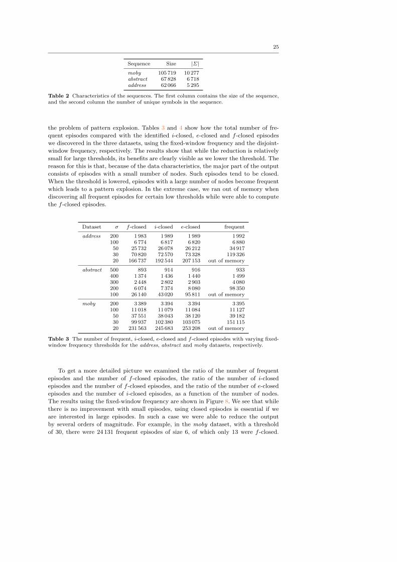
The characteristics of datasets are given in Table 22.
In the implementation an episode graph was implemented using sparse notation:
the neighbourhood of a node was presented as a list of edges. To ensure efficient scan-
ning, the sequence was implemented as a set of linked lists, one for each symbol. The
experiments were conducted on a computer with an AMD Athlon 64 processor and
2GB memory. The code was compiled with G++ 4.3.4.
We used a window of size 15 for all our experiments and varied the frequency
threshold σ. The main goal of our experiments was to demonstrate how we tackle
4 The C++ implementation is given at http://adrem.ua.ac.be/implementations/http://adrem.ua.ac.be/implementations/5 taken from http://www.bartleby.com/124/pres68http://www.bartleby.com/124/pres686 taken from http://www.gutenberg.org/etext/15http://www.gutenberg.org/etext/157 taken from http://kdd.ics.uci.edu/databases/nsfabs/nsfawards.htmlhttp://kdd.ics.uci.edu/databases/nsfabs/nsfawards.html8 http://tartarus.org/~martin/PorterStemmer/http://tartarus.org/~martin/PorterStemmer/
25
Sequence Size |Σ|
moby 105 719 10 277abstract 67 828 6 718address 62 066 5 295
Table 2 Characteristics of the sequences. The first column contains the size of the sequence,and the second column the number of unique symbols in the sequence.
the problem of pattern explosion. Tables 33 and 44 show how the total number of fre-
quent episodes compared with the identified i-closed, e-closed and f -closed episodes
we discovered in the three datasets, using the fixed-window frequency and the disjoint-
window frequency, respectively. The results show that while the reduction is relatively
small for large thresholds, its benefits are clearly visible as we lower the threshold. The
reason for this is that, because of the data characteristics, the major part of the output
consists of episodes with a small number of nodes. Such episodes tend to be closed.
When the threshold is lowered, episodes with a large number of nodes become frequent
which leads to a pattern explosion. In the extreme case, we ran out of memory when
discovering all frequent episodes for certain low thresholds while were able to compute
the f -closed episodes.
Dataset σ f -closed i-closed e-closed frequent
address 200 1 983 1 989 1 989 1 992100 6 774 6 817 6 820 6 88050 25 732 26 078 26 212 34 91730 70 820 72 570 73 328 119 32620 166 737 192 544 207 153 out of memory
abstract 500 893 914 916 933400 1 374 1 436 1 440 1 499300 2 448 2 802 2 903 4 080200 6 074 7 374 8 080 98 350100 26 140 43 020 95 811 out of memory
moby 200 3 389 3 394 3 394 3 395100 11 018 11 079 11 084 11 12750 37 551 38 043 38 120 39 18230 99 937 102 380 103 075 151 11520 231 563 245 683 253 208 out of memory
Table 3 The number of frequent, i-closed, e-closed and f -closed episodes with varying fixed-window frequency thresholds for the address, abstract and moby datasets, respectively.
To get a more detailed picture we examined the ratio of the number of frequent
episodes and the number of f -closed episodes, the ratio of the number of i-closed
episodes and the number of f -closed episodes, and the ratio of the number of e-closed
episodes and the number of i-closed episodes, as a function of the number of nodes.
The results using the fixed-window frequency are shown in Figure 88. We see that while
there is no improvement with small episodes, using closed episodes is essential if we
are interested in large episodes. In such a case we were able to reduce the output
by several orders of magnitude. For example, in the moby dataset, with a threshold
of 30, there were 24 131 frequent episodes of size 6, of which only 13 were f -closed.
26
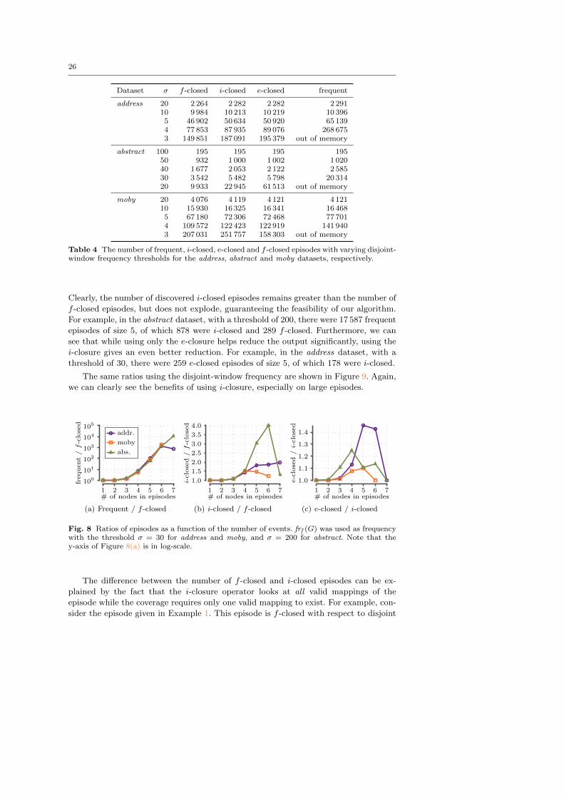
Dataset σ f -closed i-closed e-closed frequent
address 20 2 264 2 282 2 282 2 29110 9 984 10 213 10 219 10 3965 46 902 50 634 50 920 65 1394 77 853 87 935 89 076 268 6753 149 851 187 091 195 379 out of memory
abstract 100 195 195 195 19550 932 1 000 1 002 1 02040 1 677 2 053 2 122 2 58530 3 542 5 482 5 798 20 31420 9 933 22 945 61 513 out of memory
moby 20 4 076 4 119 4 121 4 12110 15 930 16 325 16 341 16 4685 67 180 72 306 72 468 77 7014 109 572 122 423 122 919 141 9403 207 031 251 757 158 303 out of memory
Table 4 The number of frequent, i-closed, e-closed and f -closed episodes with varying disjoint-window frequency thresholds for the address, abstract and moby datasets, respectively.
Clearly, the number of discovered i-closed episodes remains greater than the number of
f -closed episodes, but does not explode, guaranteeing the feasibility of our algorithm.
For example, in the abstract dataset, with a threshold of 200, there were 17 587 frequent
episodes of size 5, of which 878 were i-closed and 289 f -closed. Furthermore, we can
see that while using only the e-closure helps reduce the output significantly, using the
i-closure gives an even better reduction. For example, in the address dataset, with a
threshold of 30, there were 259 e-closed episodes of size 5, of which 178 were i-closed.
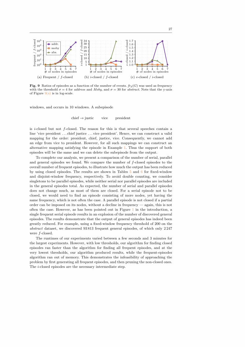
The same ratios using the disjoint-window frequency are shown in Figure 99. Again,
we can clearly see the benefits of using i-closure, especially on large episodes.
1 2 3 4 5 6 7
100101102103104105
# of nodes in episodes
frequent/f-closed
addr.
moby
abs.
(a) Frequent / f -closed
1 2 3 4 5 6 7
1.0
1.5
2.0
2.5
3.0
3.5
4.0
# of nodes in episodes
i-closed
/f-closed
(b) i-closed / f -closed
1 2 3 4 5 6 7
1.0
1.1
1.2
1.3
1.4
# of nodes in episodes
e-closed
/i-closed
(c) e-closed / i-closed
Fig. 8 Ratios of episodes as a function of the number of events. frf (G) was used as frequencywith the threshold σ = 30 for address and moby, and σ = 200 for abstract. Note that they-axis of Figure 8(a)8(a) is in log-scale.
The difference between the number of f -closed and i-closed episodes can be ex-
plained by the fact that the i-closure operator looks at all valid mappings of the
episode while the coverage requires only one valid mapping to exist. For example, con-
sider the episode given in Example 11. This episode is f -closed with respect to disjoint
27
1 2 3 4 5 6 7
100101102103104105
# of nodes in episodes
frequent/f-closed
addr.
moby
abs.
(a) Frequent / f -closed
1 2 3 4 5 6 7
15
10
15
20
25
3034
# of nodes in episodes
i-closed
/f-closed
(b) i-closed / f -closed
1 2 3 4 5 6 7
1.01.11.21.31.41.51.61.7
# of nodes in episodes
e-closed
/i-closed
(c) e-closed / i-closed
Fig. 9 Ratios of episodes as a function of the number of events. frd (G) was used as frequencywith the threshold σ = 4 for address and Moby, and σ = 30 for abstract. Note that the y-axisof Figure 9(a)9(a) is in log-scale.
windows, and occurs in 10 windows. A subepisode
chief→ justic vice president
is i-closed but not f -closed. The reason for this is that several speeches contain a
line ’vice president . . . chief justice . . . vice president’. Hence, we can construct a valid
mapping for the order: president, chief, justice, vice. Consequently, we cannot add
an edge from vice to president. However, for all such mappings we can construct an
alternative mapping satisfying the episode in Example 11. Thus the support of both
episodes will be the same and we can delete the subepisode from the output.
To complete our analysis, we present a comparison of the number of serial, parallel
and general episodes we found. We compare the number of f -closed episodes to the
overall number of frequent episodes, to illustrate how much the output has been reduced
by using closed episodes. The results are shown in Tables 55 and 66 for fixed-window
and disjoint-window frequency, respectively. To avoid double counting, we consider
singletons to be parallel episodes, while neither serial nor parallel episodes are included
in the general episodes total. As expected, the number of serial and parallel episodes
does not change much, as most of them are closed. For a serial episode not to be
closed, we would need to find an episode consisting of more nodes, yet having the
same frequency, which is not often the case. A parallel episode is not closed if a partial
order can be imposed on its nodes, without a decline in frequency — again, this is not
often the case. However, as has been pointed out in Figure 11 in the introduction, a
single frequent serial episode results in an explosion of the number of discovered general
episodes. The results demonstrate that the output of general episodes has indeed been
greatly reduced. For example, using a fixed-window frequency threshold of 200 on the
abstract dataset, we discovered 93 813 frequent general episodes, of which only 2 247
were f -closed.
The runtimes of our experiments varied between a few seconds and 3 minutes for
the largest experiments. However, with low thresholds, our algorithm for finding closed
episodes ran faster than the algorithm for finding all frequent episodes, and at the
very lowest thresholds, our algorithm produced results, while the frequent-episodes
algorithm ran out of memory. This demonstrates the infeasibility of approaching the
problem by first generating all frequent episodes, and then pruning the non-closed ones.
The i-closed episodes are the necessary intermediate step.

28
serial serial parallel parallel general generalDataset σ f -closed frequent f -closed frequent f -closed frequent
address 200 293 293 1 670 1 674 20 25100 1 739 1 742 4 846 4 878 189 26050 8 436 8 494 15 526 16 068 1 770 10 35530 24 620 24 973 36 593 41 055 9 607 53 29820 61 254 N/A 67 658 N/A 37 825 N/A
abstract 500 116 116 667 669 110 148400 206 208 939 942 229 349300 433 448 1 435 1 471 580 2 161200 1 124 1 353 2 703 3 184 2 247 93 813100 4 597 N/A 7 854 N/A 13 689 N/A
moby 200 594 594 2 772 2 776 23 25100 2 992 2 997 7 749 7 788 277 34250 12 529 12 583 22 615 23 192 2 407 3 40730 34 469 34 915 52 481 58 021 12 987 58 17920 85 112 N/A 96 675 N/A 49 866 N/A
Table 5 The number of f -closed and frequent serial, parallel and general episodes, withvarying fixed-window frequency thresholds for the address, abstract and moby datasets, re-spectively. Singletons are classified as parallel episodes, and general episodes do not includethe serial and parallel episodes.
serial serial parallel parallel general generalDataset σ f -closed frequent f -closed frequent f -closed frequent
address 20 479 479 1 744 1 753 41 5910 3 004 3 012 6 325 6 468 655 9165 15 318 15 557 24 038 27 069 7 546 22 5134 25 532 26 372 36 116 45 108 16 205 197 1953 49 859 N/A 57 293 N/A 42 699 N/A
abstract 100 20 20 160 160 15 1550 164 166 565 573 203 28140 300 314 892 924 485 1 34730 631 708 1 479 1 660 1 432 17 94620 1 638 N/A 2 920 N/A 5 375 N/A
moby 20 1 010 1 014 2 983 3 004 83 10310 5 075 5 099 9 853 10 035 1 002 1 3345 22 016 22 304 34 070 37 920 11 094 17 4774 35 950 36 807 50 545 61 704 23 077 43 4293 69 048 N/A 79 944 N/A 58 039 N/A
Table 6 The number of f -closed and frequent serial, parallel and general episodes, withvarying disjoint-window frequency thresholds for the address, abstract and moby datasets,respectively. Singletons are classified as parallel episodes, and general episodes do not includethe serial and parallel episodes.
9 Related Work
Searching for frequent patterns in data is a very common data mining problem. The first
attempt at discovering sequential patterns was made by Wang et al. [1919]. There, the
dataset consists of a number of sequences, and a pattern is considered interesting if it is
long enough and can be found in a sufficient number of sequences. The method proposed
in this paper, however, was not guaranteed to discover all interesting patterns, but a
29
complete solution to a more general problem (dropping the pattern length constraint)
was later provided by Agrawal and Srikant [22] using an Apriori-style algorithm [11].
It has been argued that not all discovered patterns are of interest to the user,
and some research has gone into outputting only closed sequential patterns, where
a sequence is considered closed if it is not properly contained in any other sequence
which has the same frequency. Yan et al. [2121], Tzvetkov et al. [1818], and Wang and
Han [2020] proposed methods for mining such closed patterns, while Garriga [55] further
reduced the output by post-processing it and representing the patterns using partial
orders. Despite their name, the patterns discovered by Garriga are different from the
traditional episodes. A sequence covers an episode if every node of the DAG can be
mapped to a symbol such that the order is respected, whereas a partial order discovered
by Garriga is covered by a sequence if all paths in the DAG occur in the sequence;
however, a single event in a sequence can be mapped to multiple nodes.
In another attempt to trim the output, Garofalakis et al. [77] proposed a family of
algorithms called Spirit which allow the user to define regular expressions that specify
the language that the discovered patterns must belong to.
Looking for frequent episodes in a single event sequence was first proposed by
Mannila et al. [1212]. The Winepi algorithm finds all episodes that occur in a sufficient
number of windows of fixed length. The frequency of an episode is defined as the fraction
of all fixed-width sliding windows in which the episode occurs. The user is required to
choose the width of the window and a frequency threshold. Specific algorithms are
given for the case of parallel and serial episodes. However, no algorithm for detecting
general episodes (DAGs) is provided.
The same paper proposes the Minepi method, where the interestingness of an
episode is measured by the number of minimal windows that contain it. As was shown
by Tatti [1616], Minepi fails due to an error in its definition. Zhou et al. [2222] proposed
mining closed serial episodes based on the Minepi method, without solving this er-
ror. Laxman et al. introduced a monotonic measure as the maximal number of non-
overlapping occurrences of the episode [1111].
Pei et al. [1515] considered a restricted version of our problem setup. In their setup,
items are allowed to occur only once in a window (string in their terminology). This
means that the discovered episodes can contain only one occurrence of each item. This
restriction allows them to easily construct closed episodes. Our setup is more general
since we do not restrict the number of occurrences of a symbol in the window and the
miner introduced by Pei cannot be adapted to our problem setting since the restriction
imposed by the authors plays a vital part in their algorithm.
Garriga [44] pointed out that Winepi suffers from bias against longer episodes, and
proposed solving this by increasing the window length proportionally to the episode
length. However, as was pointed out by Meger and Rigotti [1313], the algorithm given in
this paper contained an error.
An attempt to define frequency without using any windows has been made by
Calders et al. [33] where the authors define an interestingness measure of an itemset
in a stream to be the frequency starting from a point in time that maximizes it.
However, this method is defined only for itemsets, or parallel episodes, and not for
general episodes. Cule et al. [66] proposed a method that uses neither a window of
fixed size, nor minimal occurrences, and an interestingness measure is defined as a
combination of the cohesion and the frequency of an episode — again, only for parallel
episodes. Tatti [1616] and Gwadera et al. [88, 99] define an episode as interesting if its
occurrences deviate from expectations.
30
Finally, an extensive overview of temporal data mining has been made by Laxman
and Sastry [1010].
10 Conclusions
In this paper, we tackled the problem of pattern explosion when mining frequent
episodes in an event sequence. In such a setting, much of the output is redundant,
as many episodes have the same frequency as some other, more specific, episodes. We
therefore output only closed episodes, for which this is not the case. Further redun-
dancy is found in the fact that some episodes can be represented in more than one way.
We solve this problem by restricting ourselves to strict, transitively closed episodes.
Defining frequency-closed episodes created new problems, as, unlike in some other
settings, a non-closed frequent episode can have more than one closure. To solve this,
we defined a closure operator based on instances. This closure does not suffer from
the same problems that occur with the closure based on frequency. Unlike the closure
based on frequency, an episode will always have only one instance-closure.
We further proved that every f -closed episode must also be i-closed. Based on this,
we developed an algorithm that efficiently identifies i-closed episodes, as well as f -closed
episodes, in a post-processing step. Experiments have confirmed that the reduction in
output is considerable, and essential for large episodes, where we reduced the output by
several orders of magnitude. Moreover, thanks to introducing i-closed episodes, we can
now produce output for thresholds at which finding all frequent episodes is infeasible.
Acknowledgments
Nikolaj Tatti is supported by a Post-doctoral Fellowship of the Research Foundation
Flanders (fwo).
References
1. Rakesh Agrawal and Ramakrishnan Srikant. Fast algorithms for mining association rules.In Proceedings of the 20th International Conference on Very Large Data Bases (VLDB1994), pages 487–499, 1994.
2. Rakesh Agrawal and Ramakrishnan Srikant. Mining sequential patterns. 11th Interna-tional Conference on Data Engineering (ICDE 1995), 0:3–14, 1995.
3. Toon Calders, Nele Dexters, and Bart Goethals. Mining frequent itemsets in a stream.In Proceedings of the 7th IEEE International Conference on Data Mining (ICDM 2007),pages 83–92, 2007.
4. Gemma Casas-Garriga. Discovering unbounded episodes in sequential data. In KnowledgeDiscovery in Databases: PKDD 2003, 7th European Conference on Principles and Practiceof Knowledge Discovery in Databases, pages 83–94, 2003.
5. Gemma Casas-Garriga. Summarizing sequential data with closed partial orders. In Pro-ceedings of the SIAM International Conference on Data Mining (SDM 2005), pages 380–391, 2005.
6. Boris Cule, Bart Goethals, and Celine Robardet. A new constraint for mining sets insequences. In Proceedings of the SIAM International Conference on Data Mining (SDM2009), pages 317–328, 2009.
7. Minos Garofalakis, Rajeev Rastogi, and Kyuseok Shim. Mining sequential patterns withregular expression constraints. IEEE Transactions on Knowledge and Data Engineering,14(3):530–552, 2002.
31
8. Robert Gwadera, Mikhail J. Atallah, and Wojciech Szpankowski. Markov models foridentification of significant episodes. In Proceedings of the SIAM International Conferenceon Data Mining (SDM 2005), pages 404–414, 2005.
9. Robert Gwadera, Mikhail J. Atallah, and Wojciech Szpankowski. Reliable detection ofepisodes in event sequences. Knowledge and Information Systems, 7(4):415–437, 2005.
10. Srivatsan Laxman and P. S. Sastry. A survey of temporal data mining. SADHANA,Academy Proceedings in Engineering Sciences, 31(2):173–198, 2006.
11. Srivatsan Laxman, P. S. Sastry, and K. P. Unnikrishnan. A fast algorithm for findingfrequent episodes in event streams. In Proceedings of the 13th ACM SIGKDD InternationalConference on Knowledge discovery and data mining (KDD 2007), pages 410–419, 2007.
12. Heikki Mannila, Hannu Toivonen, and A. Inkeri Verkamo. Discovery of frequent episodesin event sequences. Data Mining and Knowledge Discovery, 1(3):259–289, 1997.
13. Nicolas Meger and Christophe Rigotti. Constraint-based mining of episode rules andoptimal window sizes. In Knowledge Discovery in Databases: PKDD 2004, 8th EuropeanConference on Principles and Practice of Knowledge Discovery in Databases, pages 313–324, 2004.
14. Nicolas Pasquier, Yves Bastide, Rafik Taouil, and Lotfi Lakhal. Discovering frequentclosed itemsets for association rules. In ICDT ’99: Proceedings of the 7th InternationalConference on Database Theory, pages 398–416, 1999.
15. Jian Pei, Haixun Wang, Jian Liu, Ke Wang, Jianyong Wang, and Philip S. Yu. Discoveringfrequent closed partial orders from strings. IEEE Transactions on Knowledge and DataEngineering, 18(11):1467–1481, 2006.
16. Nikolaj Tatti. Significance of episodes based on minimal windows. In Proceedings of the9th IEEE International Conference on Data Mining (ICDM 2009), pages 513–522, 2009.
17. Nikolaj Tatti and Boris Cule. Mining closed strict episodes. In Proceedings of the 10thIEEE International Conference on Data Mining (ICDM 2010), pages 501–510, 2010.
18. Petre Tzvetkov, Xifeng Yan, and Jiawei Han. Tsp: Mining top-k closed sequential patterns.In Proceedings of the 3rd IEEE International Conference on Data Mining (ICDM 2003),pages 347–354, 2003.
19. Jason Tsong-Li Wang, Gung-Wei Chirn, Thomas G. Marr, Bruce Shapiro, Dennis Shasha,and Kaizhong Zhang. Combinatorial pattern discovery for scientific data: some preliminaryresults. ACM SIGMOD Record, 23(2):115–125, 1994.
20. Jianyong Wang and Jiawei Han. Bide: Efficient mining of frequent closed sequences. 20thInternational Conference on Data Engineering (ICDE 2004), 0:79, 2004.
21. Xifeng Yan, Jiawei Han, and Ramin Afshar. Clospan: Mining closed sequential patternsin large datasets. In Proceedings of the SIAM International Conference on Data Mining(SDM 2003), pages 166–177, 2003.
22. Wenzhi Zhou, Hongyan Liu, and Hong Cheng. Mining closed episodes from event sequencesefficiently. In Proceedings of the 14th Pacific-Asia Conference on Knowledge Discoveryand Data Mining(1), pages 310–318, 2010.