Mining Periodic Cliques in Temporal Networks

Hongchao Qin†, Rong-Hua Li‡, Guoren Wang‡, Lu Qin#, Yurong Cheng‡, Ye Yuan††Northeastern University, China; ‡Beijing Institute of Technology, China; #University of Technology Sydney, Australia

{qhc.neu;lironghuascut}@gmail.com; wanggrbit@126.com; Lu.Qin@uts.edu.au; yrcheng@bit.edu.cn; yuanye@mail.neu.edu.cn

Abstract—Periodicity is a frequently happening phenomenonfor social interactions in temporal networks. Mining periodiccommunities are essential to understanding periodic group behav-iors in temporal networks. Unfortunately, most previous studiesfor community mining in temporal networks ignore the periodicpatterns of communities. In this paper, we study a problemof seeking periodic communities in a temporal network, whereeach edge is associated with a set of timestamps. We propose anovel model, called maximal σ-periodic k-clique, that representsa periodic community in temporal networks. Specifically, amaximal σ-periodic k-clique is a clique with size larger thank that appears at least σ times periodically in the temporalgraph. We show that the problem of enumerating all thoseperiodic cliques is NP-hard. To compute all of them efficiently,we first develop two effective graph reduction techniques tosignificantly prune the temporal graph. Then, we present anefficient enumeration algorithm to enumerate all maximal σ-periodic k-cliques in the reduced graph. The results of extensiveexperiments on five real-life datasets demonstrate the efficiency,scalability, and effectiveness of our algorithms.

I. INTRODUCTION

In many real-life networks, such as communication net-works, scientific collaboration networks, and social networks,the links are often associated with temporal information. Forexample, in a face-to-face contact network [1], [2], eachedge (u, v, t) denotes a contact between two individuals uand v at time t. In an email communication network, eachemail contains a sender and a receiver, as well as the timewhen the email was sent. In a scientific collaboration network(e.g., DBLP), each edge (u, v, t) represents that two authorsu and v coauthored a paper at time t. The networks thatinvolve temporal information are typically termed as temporalnetworks [3]–[5].

Periodicity is a frequently happening phenomenon for socialinteractions in temporal networks. Weekly group meeting,monthly birthday party, and yearly family reunions − theseare regular and significant patterns in temporal interactionnetworks. Mining such periodic group patterns are essential tounderstanding and predicting group behaviors in a temporalnetwork. In this paper, we investigate a novel data miningproblem for temporal networks: periodic community mining,or the detection of all communities that occur at regulartime intervals, and show that the proposed technique can beapplied to discover the inherent periodicity of communities ina temporal network. Mining the periodic community patternscould be very useful for many practical applications, two ofwhich are listed as follows.Periodic movement behavior discovery. Consider an appli-cation in studying the collective movement behaviors of wildherds of animals [6]. It is well known that the movementbehavior of wild herds of animals often exhibits periodicgroup patterns. In practice, ecologists can tag the animals withtracking sensors to study the collective movement patterns ofthe animals. In this application, the interactions of the animals(e.g., two animals within a short distance may be considered

as an interaction) can be modeled as a temporal network. Bymining periodic communities in this temporal network, we areable to identify periodic group movement behaviors of wildanimals. Mining such periodic group movement behavior ofwild animals can be of ecological interests [6]. For example,if a herd of animals fail to follow the periodic mitigationbehavior, it could be a signal of abnormal environment change.Predicting future activities. Periodic pattern is a predictablepattern, because it repeatedly occurs at regular time intervals.Once we identify a periodic activity, we may predict thesame activity will appear within a regular time interval. Basedon this observation, we are capable of inferring the futureinteractions of a group of individuals in a temporal networkby mining periodic communities. Taking a temporal scientificcollaboration network DBLP as an example, suppose that fourresearchers A,B,C, and D in DBLP have collaborated witheach other in 2015, 2016, and 2017 years. Then, we can inferthat these four researchers are likely to coauthor papers in2018 year.

Recently, the problem of mining communities on temporalgraphs has attracted much attention due to numerous appli-cations [4], [5], [7]. For example, Wu et al. [7] proposeda temporal k-core model to find cohesive subgraphs in atemporal network. Ma et al. [4] devised a dense subgraphmining algorithm to identify cohesive subgraphs in a temporalnetwork. Li et al. [5] developed an algorithm to detect persis-tent communities in a temporal graph. All these communitymining algorithms do not consider the periodic patterns ofcommunities, thus cannot be applied to identify periodiccommunities. To the best of our knowledge, we are the firstto study the periodic community mining problem, define theperiodic clique model and propose efficient solutions to findperiodic cliques in temporal graphs. The main contributionsof our work are summarized as follows.Novel model. We propose a novel maximal σ-periodic k-clique model to characterize periodic communities in a tem-poral graph, since the clique is the most cohesive structurein a graph and it is a traditional model for community. Weshow that the traditional maximal clique problem is a specialcase of the problem of enumerating all maximal σ-periodic k-cliques in a temporal graph. Since the problem of enumeratingmaximal cliques is NP-hard [8], our problem is also NP-hard.New algorithms. First, we develop two novel relaxed periodicclique models, called WPCore and SPCore, based on the con-cept of k-core [9]. On the basis of the WPCore and SPCore,we develop two efficient and powerful graph reduction tech-niques to prune the input temporal graph. We show that bothWPCore and SPCore can be computed in near-linear timeand space complexity. Second, we propose an enumerationalgorithm based on a carefully-design graph transformationtechnique to efficiently enumerate all maximal σ-periodic k-cliques. In addition, we present a theoretical analysis for the

number of such cliques in a temporal graph based on a newly-proposed concept called σ-periodic degeneracy δ. We alsoshow that the problem of enumerating all maximal σ-periodick-cliques is fixed-parameter tractable with respect to δ, whichis often very small in practice as confirmed in our experiments.Extensive experimental results. We conduct comprehensiveexperiments on five real-life temporal networks. The resultsshow that our best algorithm is much faster than the baselineson all datasets under most parameter settings. For example, ourbest algorithm can identify all maximal σ-periodic k-cliquesin around 400 seconds on a large temporal graph with morethan 1.7 million nodes and 12 million edges. The baselinealgorithm, however, cannot get the results in 2 days. We alsoexamine two case studies to evaluate the effectiveness of ourmodel. The results show that our model is indeed able toidentify many interesting periodic communities that can notbe found by the other models.Organization. Section II introduces the model of maximalσ-periodic k-clique and formulates our problem. The graphreduction techniques are proposed in Section III. Section IVproposes the enumeration algorithm and presents an analysisof the number of those cliques. The experiments are shownin Section V. We review the related work in Section VI, andconclude this work in Section VII.

II. PRELIMINARIES

Let G = (V, E) be an undirected temporal graph, where Vand E denote the set of nodes and the set of temporal edgesrespectively. Let n = |V| and m = |E| be the number ofnodes and temporal edges respectively. Each temporal edgee ∈ E is a triplet (u, v, t), where u, v are nodes in V , and t isthe interaction time between u and v. We assume that t is aninteger, because the timestamp is an integer in practice. For atemporal graph G, the de-temporal graph of G denoted by G =(V,E) is a graph that ignores all the timestamps associatedwith the temporal edges. More formally, for the de-temporalgraph G of G, we have V = V and E = {(u, v)|(u, v, t) ∈ E}.Let Nu(G) = {v|(u, v) ∈ E} be the set of neighbor nodes ofu, and du(G) = |Nu(G)| be the degree of u in G. A graphS = (VS , ES) is called a subgraph of G = (V,E) if VS ⊆ Vand ES ⊆ E. A subgraph S = (VS , ES) is referred to as aninduced subgraph of G if ES = {(u, v)|u, v ∈ VS , (u, v) ∈E}. Similarly, a temporal subgraph S = (VS , ES) is referredto as an induced temporal subgraph of G if VS ⊆ V andES = {(u, v, t)|u, v ∈ VS , (u, v, t) ∈ E}. For convenience, weuse the notion S ⊆ G (S ⊂ G if S 6= G) to represent that Sis a subgraph of G.

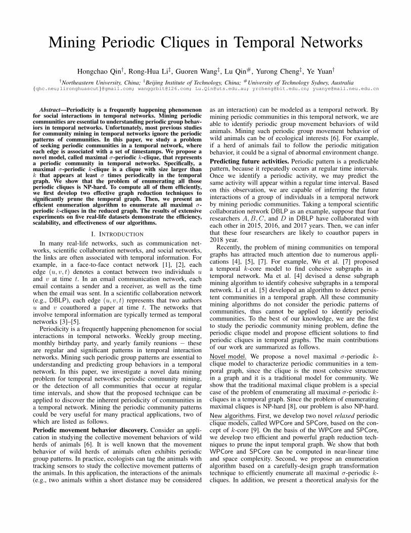
Given a temporal graph G, we can extract a series ofsnapshots based on the timestamps. Let T = {t|(u, v, t) ∈ E}be the set of timestamps. For each ti ∈ T , we can obtain asnapshot Gi = (Vi, Ei) where Vi = {u|(u, v, ti) ∈ E} andEi = {(u, v)|(u, v, ti) ∈ E}. In the rest of this paper, weassume without loss of generality that all the timestamps aresorted in a chronological order, i.e., t1 < t2 < · · · < t|T |.Fig. 1(a) illustrates a temporal graph G with 5 nodes and 22temporal edges. Figs.1(b) and (c) illustrates the de-temporalgraph of G and all the five snapshots of G respectively.

Definition 1 (time support set): Given a temporal graph G,the time support set of a subgraph S is defined as T (S) ,{ti|S ⊆ Gi}, where Gi is the i-th snapshot of G.

Definition 2 (σ-periodic time support set): Given a temporalgraph G and a parameter σ, a σ-periodic time support set of

4 ...2 31 5

v2v1

v3v1

v3v2

v4v3

v5v3

v5v4

v2v1

v3v1

v3v2

v4v3

v5v3

v5v4

v3v1

v3v2

v4v3

v5v3

v5v4

v2v1

v3v1

v3v2

v4v3

v5v3

v5v4

v1v2

v3

{2,3,4}

{1,3,5}

(a) A temporal graph G

v5v4

v1v2

v3

(b) The de-temporal graph G

v1v2 v1v2 v1v1

v3

v5v4

v3

v5v4

v3

v5v4

v3

v5

v2

v3

G1 G2 G3 G4 G5

v2

v4

(c) The five snapshots of GFig. 1. Basic concepts of the temporal graph

a subgraph S, denoted by πσ(S), is a subset of T (S) suchthat (1) πσ(S) = {tj1 , · · · , tjσ}, and (2) tji+1 − tji = p forall i = 1, · · · , σ − 1 with any constant p.

By Definition 2, we can see that the timestamps of a σ-periodic time support set forms an arithmetic sequence andthe cardinality of a σ-periodic time support set is exactly equalto σ. Clearly, there may exist many σ-periodic time supportsets for a subgraph S. Based on Definition 2, we define theσ-periodic subgraph below.

Definition 3 (σ-periodic subgraph): Given a temporal graphG, its de-temporal graph G, and a parameter σ, a subgraph Sof G is called a σ-periodic subgraph if there exists a σ-periodictime support set πσ(S) for S.

By Definition 3, any σ-periodic subgraph S ⊆ G has atleast one σ-periodic time support set πσ(S). A subgraph S isa maximal σ-periodic subgraph if there is no other σ-periodicsubgraph S′ that satisfies S ⊂ S′. Based on the widely-usedclique model, we propose a novel σ-periodic k-clique modelto define the periodic communities as follows.

Definition 4 (σ-periodic k-clique): A σ-periodic k-clique Cis a subgraph of the de-temporal graph G such that (1) C is aclique in G with |C| > k, and (2) C is a σ-periodic subgraph.

Note that for a typical temporal graph, many σ-periodiccliques are small and may not be interesting to the users.Therefore, it will be more useful to find large σ-periodiccliques for practical applications. As a result, we focus mainlyon mining the σ-periodic cliques with size larger than k asdefined in Definition 4. Based on Definition 4, we define themaximal σ-periodic k-clique as follows.

Definition 5 (maximal σ-periodic k-clique): A σ-periodick-clique C is maximal if there is no other σ-periodic k-cliqueC ′ meeting C ⊂ C ′.

For convenience, in the rest of this paper, the maximal σ-periodic k-clique is abbreviated as MPClique. Below, we usean example to illustrate the above definitions.

Example 1: Consider a temporal graph in Fig. 1(a). Supposethat σ = 3, k = 2. For the subgraph S = {(v1, v3), (v2, v3)},the time support set of S is {1, 3, 4, 5}. Clearly, by Def-inition 2, the set {1, 3, 5} is a σ-periodic time supportset of S. Therefore, the subgraph S is a σ-periodic sub-graph by Definition 3. Note that S is not a maximal σ-periodic subgraph because there is a σ-periodic subgraph C ={(v1, v3), (v2, v3), (v1, v2)} that contains S. By Definition 4,we can see that C is a σ-periodic k-clique. Moreover, it iseasy to check that C is also a maximal σ-periodic k-clique.

Based on Definition 5, we formulate the periodic communitymining problem as follows.

Problem formulation. Given a temporal graph G and param-eters σ and k, the goal of the periodic community miningproblem is to enumerate all the maximal σ-periodic k-cliques(MPCliques) in G.Hardness and challenges. We can show that the traditionalmaximal clique enumeration problem is a special case of themaximal σ-periodic k-clique enumeration problem. Considera temporal graph G that contains a set of snapshots G =Gi = G2 =, · · · ,= G|T |. Clearly, in this temporal graph G,every subgraph of G is periodic. As a result, the problemof enumerating all maximal σ-periodic k-cliques is equivalentto the problem of enumerating all maximal cliques (with sizelarger than k) in the de-temporal graph G. Since the traditionalmaximal clique enumeration problem is known to be NP-hard,our problem is also NP-hard.

Although there is a close connection between our problemand the maximal clique enumeration problem, the existingmaximal clique enumeration algorithms cannot be directlyapplied to solve our problem. The reason is that the traditionalmaximal clique enumeration algorithms, such as the Bron-Kerbosch algorithm [10] can only identify maximal cliquesin a snapshot Gi for the timestamp ti. It is not clearlyhow to apply this algorithm to derive maximal periodiccliques. To solve our problem, a possible solution is first toenumerate all maximal cliques in the de-temporal graph, andthen checks which of them is periodic. However, this methodis quite complicated and even intractable, because a clique ina snapshot may contain a maximal periodic clique with lessnodes in a periodic time support set. Therefore, to identify allMPCliques, we need to check each sub-clique of a maximalclique in each snapshot, which is very costly. Another potentialapproach is first to enumerate all periodic subgraphs, and thenapplies a traditional maximal clique enumeration algorithm toidentify all MPCliques in each periodic subgraph. Clearly, thisapproach may involve numerous redundant computations forcliques with the same nodes, because the number of periodicsubgraphs may be very large and the same MPClique could berepeatedly enumerated in many different periodic subgraphs.Therefore, the challenge of our problem is how to efficientlyenumerate all MPCliques with less redundant computations.In the following sections, we will develop several novel graphreduction techniques and an efficient enumeration algorithmto identify all MPCliques.

III. REDUCTION BY PERIODIC CORES

In this section, we propose several powerful techniquesto prune the unpromising nodes which are definitely notcontained in any maximal periodic clique. Our key idea forgraph reduction is based on the concept of k-core [11].Before proceeding further, we first give the definition of k-core (abbreviated as KCore) as follows.

Definition 6 (KCore): Given a de-temporal graph G of Gand a parameter k, a KCore is a maximal subgraph of G inwhich every node has degree at least k, i.e., du(G) ≥ k foru ∈ G.

It is easy to check that if a node is contained in a MPClique,this node will have at least k neighbors in the de-temporalgraph G of G. Hence, if a node is not included in theKCore of G, it must be not contained in any MPClique.As a consequence, we can first prune all nodes that are notcontained in the KCore of G. This prune rule is simple, butit may be not very effective, because it does not consider theperiodic property of the MPClique for pruning. Below, we

v4v2

v1

{1

,3, 5

,7} v6

v7

v5

{1

,2, 3

,5}

v3

v8

{1,2,3,5}

{1,2,3}

{1,2} {1,3}

{2, 3}

{1,3,5,7}

Fig. 2. Running example

develop a novel concept called WPCore which can capturethe periodic property for pruning.

A. The WPCore pruning ruleBy Definitions 4 and 5, we can easily derive that every

node u in a MPClique satisfies a periodic degree property:there must exist a σ-periodic subgraph in which u has degreeno less than k. Therefore, if a node is not contained in any σ-periodic subgraph, it can be safely pruned. Since the deletionof an unpromising node may trigger its neighbors that violatethe periodic degree property, we can iteratively prune the graphuntil all nodes meet the periodic degree property. Below, wegive a definition, called (σ, k)-periodic node, to describe anode that satisfies the periodic degree property.

Definition 7 ((σ, k)-periodic node): Given a temporal graphG, its de-temporal graph G, and parameters σ and k, a nodev is called a (σ, k)-periodic node if and only if there exists aσ-periodic subgraph of G in which v has degree at least k.

Recall that by Definition 3, a σ-periodic subgraph may havemany σ-periodic time support sets. Therefore, there may alsoexist many σ-periodic time support sets for a (σ, k)-periodicnode v in which v has degree no less than k. Below, we givea definition to describe all σ-periodic time support sets for a(σ, k)-periodic node.

Based on Definition 7, we define the (σ, k)-periodic timesupport set for a (σ, k)-periodic node as follows.

Definition 8 ((σ, k)-periodic time support set): Given atemporal graph G and a (σ, k)-periodic node v, the (σ, k)-periodic time support set of v is πkσ(v) , [tj1 , · · · , tjσ ] thatsatisfies (1) tji+1

− tji = p for each i = 1, · · · , σ − 1 with aconstant p, and (2) dv(S) ≥ k, where S is a subgraph of thesnapshot Gti for each i = 1, · · · , σ − 1.

By Definition 8, for any (σ, k)-periodic node v, there is a σ-periodic subgraph S with πσ(S) = πkσ(v) in which dv(S) ≥ k.Since a σ-periodic subgraph may have many σ-periodic timesupport sets, there also exist many (σ, k)-periodic time supportsets for a (σ, k)-periodic node v. For convenience, we letPT(v) be the set of all those (σ, k)-periodic time support setsfor a node v. Clearly, a node v is a (σ, k)-periodic node if andonly if PT(v) 6= ∅. Based on the above definitions, we presenta new periodic cohesive subgraph model, called σ-periodicweak k-core (abbreviated as WPCore), which will be appliedto prune unpromising nodes in enumerating all MPCliques.The WPCore is defined as follows.

Definition 9 (σ-periodic weak k-core): Given a temporalgraph G, two integer parameters σ and k, a subset of nodesS in G is called a σ-periodic weak k-core if it meets thefollowing constraints.(1) Periodic degree constraint: each node u ∈ S is a (σ, k)-periodic node of the temporal subgraph induced by S;(2) Maximal constraint: there does not exist a subset of nodesS′ in G that satisfies (1) and S ⊂ S′.

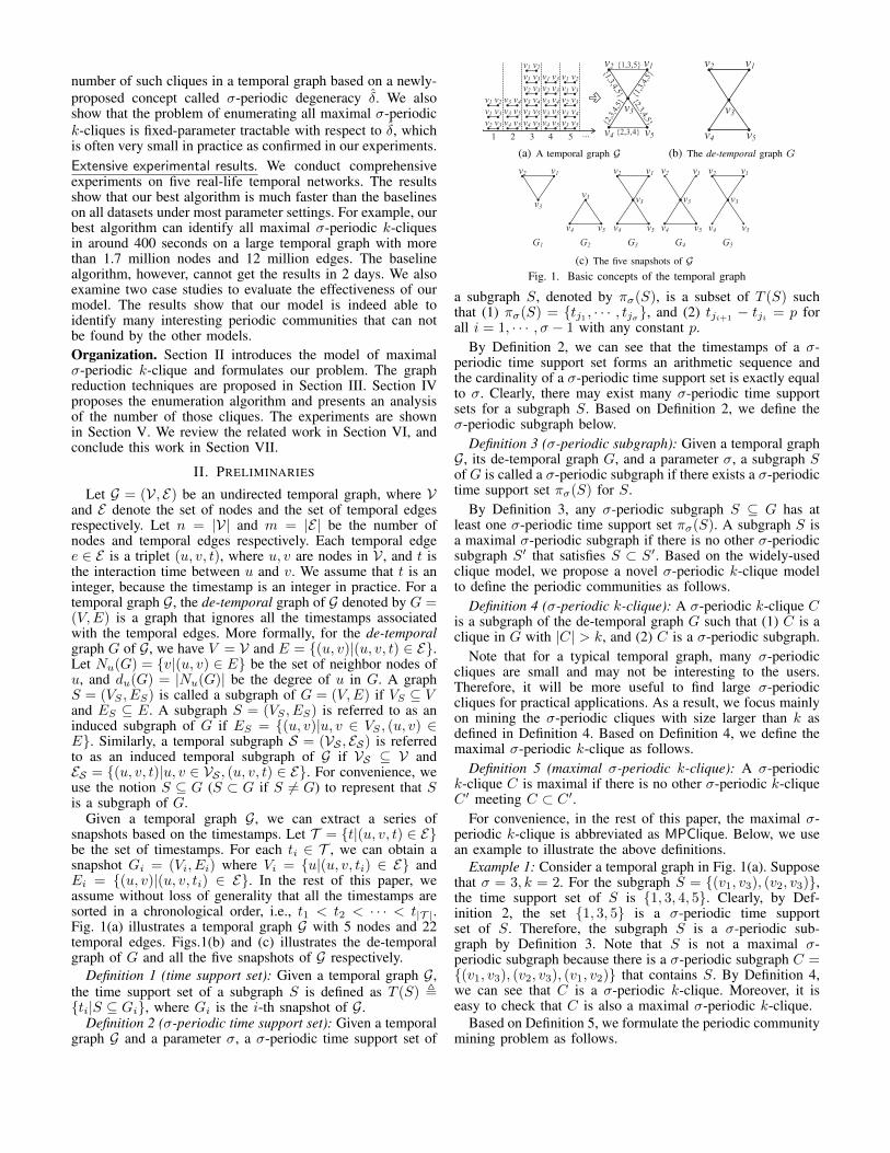
The following example illustrates the above definitions.Example 2: Consider a temporal graph G shown in Fig. 2.

Note that in Fig. 2, each temporal edge is associated witha set of integers denoting the set of timestamps of that

Algorithm 1: WPCore (G, σ, k)Input: Temporal graph G = (V, E), parameters σ and kOutput: The WPCore Vw .

1 Let G = (V,E) be the de-temporal graph of G;2 Let Gc = (Vc, Ec) be the k-core of G;3 Q ← ∅;D ← ∅;4 for u ∈ Vc do5 du(Gc)← compute the degree of u in Gc;6 (flag, PTu)←ComputePeriod (G, σ, k, u, Vc);7 if flag = 0 then8 du(Gc)← 0; Q.push(u);

9 while Q 6= ∅ do10 v ← Q.pop(); D ← D ∪ {v};11 for w ∈ Nv(Gc), s.t. du(Gc) ≥ k do12 dw(Gc)← dw(Gc)− 1;13 if dw(Gc) < k then Q.push(w);14 else15 (flag, PTw)←ComputePeriod (G, σ, k, w, Vc \D);16 if flag = 0 then17 dw(Gc)← 0; Q.push(w);

18 return Vw ← Vc \D ;

edge. Clearly, the de-temporal graph G of G is a 3-core,as every node in G has at least 3 neighbors. For node v4,we can see that it has degree no less than 3 in timestamps{1, 2, 3, 5, 7}. Suppose that σ = 3, k = 3. Then, we canderive that v4 is a (σ, k)-periodic node. This is because thereexists a σ-periodic subgraph S = {(v4, v3), (v4, v6), (v4, v7)}in which dv4(S) ≥ 3, and the corresponding (σ, k)-periodictime support set for v4 is [1, 2, 3] (i.e., πkσ(v4) = [1, 2, 3]). Itis easy to check that there are three (σ, k)-periodic time supportsets for v4 which are [1, 2, 3], [1, 3, 5] and [3, 5, 7]. Thus, wehave PT(v4) = {[1, 2, 3], [1, 3, 5], [3, 5, 7]}. Also, we can findthat v8 is not a (σ, k)-periodic node, because no σ-periodicsubgraph contains v8. By Definition 9, we can obtain that{v1, · · · , v7} is a WPCore. �

Below, we show two important properties of the WPCorewhich will be used for pruning in enumerating all MPCliques.

Lemma 3.1: Any node in a MPClique must be contained inthe WPCore of G.

Lemma 3.2: Given a temporal graph G, parameters σ andk, the WPCore is unique in G if it exists.

Based on Lemmas 3.1 and 3.2, we can first compute theWPCore S of G, and then enumerate all MPCliques on thetemporal subgraph induced by the nodes in S. The remainingquestion is how can we efficiently compute the WPCore.Below, we develop two efficient algorithms to efficientlycalculate the WPCore.The basic WPCore algorithm. Similar to the traditional k-core algorithm [9], a basic solution to compute the WPCoreis to peel the nodes from G that violate the periodic degreeproperty. Since the deletion of a node u may result in u’sneighbors no longer satisfying the periodic degree property,we need to iteratively process u’s neighbors. Such an iterativepeeling procedure terminates until no node can be deleted.When the algorithm completes, the remaining nodes form theWPCore. The detailed description of our algorithm is shownin Algorithm 1.

Algorithm 1 first computes the KCore Gc = (Vc, Ec) in thede-temporal graph (lines 1-2), because the WPCore is clearlycontained in the KCore. Then, for each node u in Vc, thealgorithm invokes Algorithm 2 to checks whether u is a (σ, k)-periodic node or not (lines 4-6). If a node u is not a (σ, k)-periodic node, it will be pushed into a queue Q (lines 7-8).

Subsequently, the algorithm iteratively processes the nodes inQ. In each iteration, the algorithm pops a node v from Qand uses a set D to maintain all the deleted nodes (line 10).For each neighbor node w of v, the algorithm updates dw(Gc)(lines 12). If the revised dw(Gc) is smaller than k, w is clearlynot a (σ, k)-periodic node. As a consequence, the algorithmpushes it into Q which will be deleted in the next iterations(line 13). Otherwise, the algorithm invokes Algorithm 2 todetermine whether w is a (σ, k)-periodic node (lines 14-15).If w is not a (σ, k)-periodic node, the algorithm sets dw(Gc)to 0, and pushes it into Q. The algorithm terminates when Qis empty. At this moment, the remaining nodes Vc \D is theWPCore of G. Below, we describe the implementation detailsof Algorithm 2.

Recall that we need to compute the set of (σ, k)-periodictime support set for a node v, i.e., PT(v), to check whether vis a (σ, k)-periodic node or not. The node v is a (σ, k)-periodicnode if and only if PT(v) is nonempty. By Definition 8,a (σ, k)-periodic time support set can be represented as anarithmetic sequence of the timestamps. In Algorithm 2, wedevise a new data structure PTv to represent the set of (σ, k)-periodic time support set for v (i.e., PT(v)). Specifically,PTv is a set where each element TS in PTv is a four-tuple[s, i, l, ArrD] representing an arithmetic sequence. In the four-tuple [s, i, l, ArrD], s denotes the starting timestamp of thearithmetic sequence, i is the common difference, l representsthe number of terms of the arithmetic sequence, and ArrD(Array of Degree) is an array that stores the degree of u ateach timestamp of the arithmetic sequence.

Based on this data structure, the algorithm makes use ofa queue PQ to maintain all the candidates of the arithmeticsequences. The algorithm also uses a set StartS to store all thestarting timestamps of the arithmetic sequences. Each elementin StartS is a two-tuple [s, d], where s denotes the startingtimestamp and d denotes the degree of u at s (lines 15-17).Initially, both PQ and StartS are set to empty sets (line 1).Then, the algorithm enumerates all the timestamps from t1to t|T | (line 2). For each timestamp, the algorithm calculatesthe number of neighbors of u (denoted by du) that are bothin Gt (the snapshot at the timestamp t) and the node setF (lines 3-4), i.e., |Nu(Gt) ∩ F |. If du ≥ k, the algorithmexplores all the candidate arithmetic sequences in PQ (lines 5-6). For each candidate TS ∈ PQ, if (t − TS.s)%TS.i = 0,we may extend the arithmetic sequence TS by t (line 7).If (t − TS.s)/TS.i 6= TS.l, we know that t cannot extendthe current arithmetic sequence TS. Since the remainingtimestamps are no less than t, they also cannot extend TS.Therefore, we can safely delete the candidate TS (lines 8-9).Otherwise, the algorithm can augment the arithmetic sequenceTS by adding t into TS. In this case, we increase TS.l by 1,and add du into the array TS.ArrD (line 8). If the augmentedarithmetic sequence TS has σ terms, TS represents a valid(σ, k)-periodic time support set for u (line 11). As a result,the algorithm adds TS into PTu and set flag to 1, denotingthat u is a (σ, k)-periodic node (line 12). At this moment,the algorithm can early terminate. Note that Algorithm 2 canalso be applied to compute the complete set of (σ, k)-periodictime support sets for u. Clearly, if t − TS.s > (σ − 1)TS.i,t cannot grow the current arithmetic sequence TS, and TSis no longer to be a valid (σ, k)-periodic time support set.Therefore, the algorithm deletes TS from PQ (line 14). Foreach starting timestamp start.s, the algorithm makes use of

Algorithm 2: ComputePeriod (G, σ, k, u, F )Input: Temporal graph G = (V, E), parameters σ, k, node u, and node set FOutput: A boolean variable flag and PT(u)

1 PQ← ∅; StartS ← ∅; PTu ← ∅; flag ← 0;2 for t← t1 : t|T | do3 Let Gt be the snapshot of G at timestamp t;4 du ← |Nu(Gt) ∩ F |;5 if du ≥ k then6 for each TS ← [s, i, l, ArrD] ∈ PQ do7 if (t− TS.s)%TS.i = 0 then8 if (t− TS.s)/TS.i 6= TS.l then9 PQ.pop(TS); continue;

10 TS.l← TS.l + 1; TS.ArrD ← TS.ArrD ∪ {du};11 if TS.l = σ then12 PTu ← PTu ∪ {TS}; flag ← 1;PQ.pop(TS);13 /* For WPCore, the algorithm can early terminate. */

14 if t− TS.s > (σ − 1)TS.i then PQ.pop(TS);

15 for start← [s, d] ∈ StartS do16 PQ.push([start.s, t− start.s, 2, {start.d, du}]);

17 StartS ← StartS ∪ {[t, du]};

18 return (flag, PTu);

the current timestamp t and start.s to generate an initialarithmetic sequence (lines 15-16). The algorithm also appliesthe current timestamp t to generate a new starting timestampwhich will be used for the next iterations (line 17). SinceAlgorithm 2 explores all the possible arithmetic sequences,it is able to correctly compute PTu. The following exampleillustrates how Algorithm 2 works.

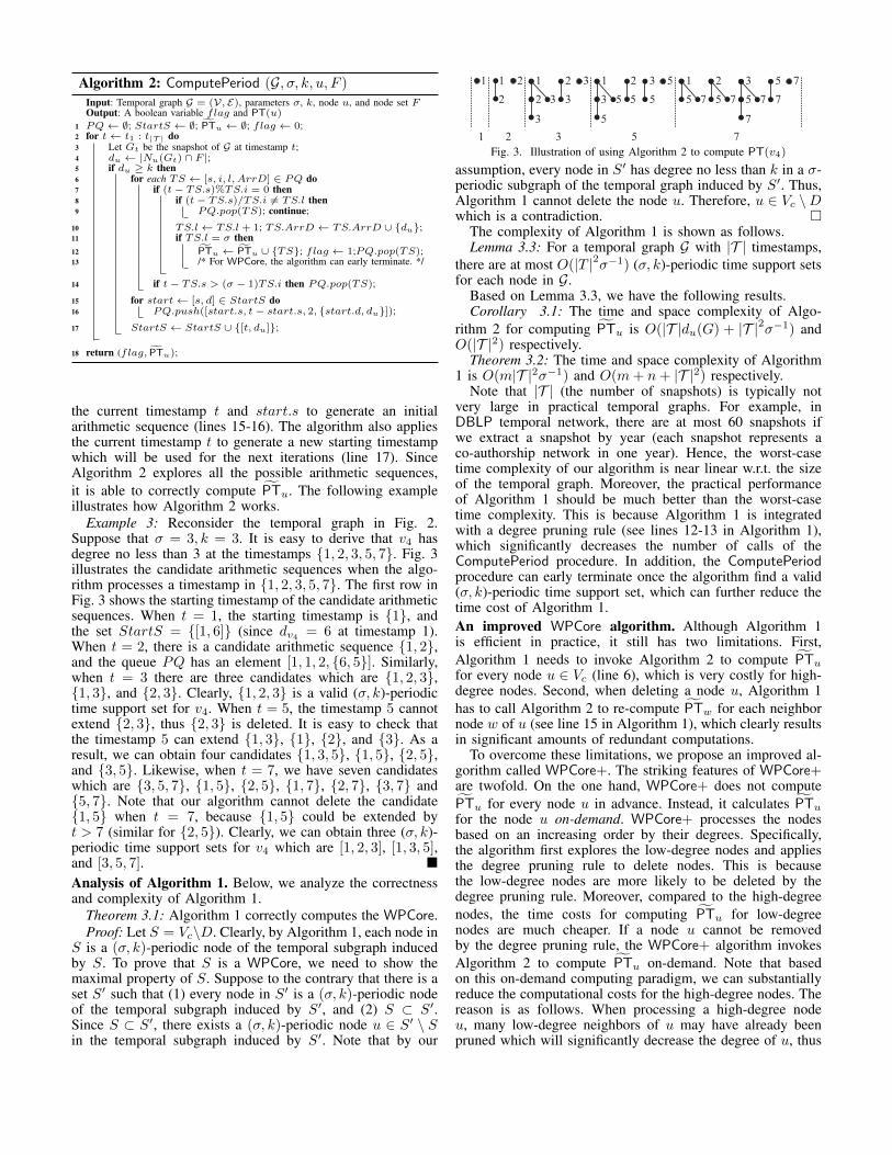
Example 3: Reconsider the temporal graph in Fig. 2.Suppose that σ = 3, k = 3. It is easy to derive that v4 hasdegree no less than 3 at the timestamps {1, 2, 3, 5, 7}. Fig. 3illustrates the candidate arithmetic sequences when the algo-rithm processes a timestamp in {1, 2, 3, 5, 7}. The first row inFig. 3 shows the starting timestamp of the candidate arithmeticsequences. When t = 1, the starting timestamp is {1}, andthe set StartS = {[1, 6]} (since dv4 = 6 at timestamp 1).When t = 2, there is a candidate arithmetic sequence {1, 2},and the queue PQ has an element [1, 1, 2, {6, 5}]. Similarly,when t = 3 there are three candidates which are {1, 2, 3},{1, 3}, and {2, 3}. Clearly, {1, 2, 3} is a valid (σ, k)-periodictime support set for v4. When t = 5, the timestamp 5 cannotextend {2, 3}, thus {2, 3} is deleted. It is easy to check thatthe timestamp 5 can extend {1, 3}, {1}, {2}, and {3}. As aresult, we can obtain four candidates {1, 3, 5}, {1, 5}, {2, 5},and {3, 5}. Likewise, when t = 7, we have seven candidateswhich are {3, 5, 7}, {1, 5}, {2, 5}, {1, 7}, {2, 7}, {3, 7} and{5, 7}. Note that our algorithm cannot delete the candidate{1, 5} when t = 7, because {1, 5} could be extended byt > 7 (similar for {2, 5}). Clearly, we can obtain three (σ, k)-periodic time support sets for v4 which are [1, 2, 3], [1, 3, 5],and [3, 5, 7]. �

Analysis of Algorithm 1. Below, we analyze the correctnessand complexity of Algorithm 1.

Theorem 3.1: Algorithm 1 correctly computes the WPCore.Proof: Let S = Vc\D. Clearly, by Algorithm 1, each node in

S is a (σ, k)-periodic node of the temporal subgraph inducedby S. To prove that S is a WPCore, we need to show themaximal property of S. Suppose to the contrary that there is aset S′ such that (1) every node in S′ is a (σ, k)-periodic nodeof the temporal subgraph induced by S′, and (2) S ⊂ S′.Since S ⊂ S′, there exists a (σ, k)-periodic node u ∈ S′ \ Sin the temporal subgraph induced by S′. Note that by our

31 2 5 7

1 1

2

2 1

2

32

3

3

3

5

5 3

5

75

7

7

1 2

3 53 5

1

5

2

5 77 7

5

Fig. 3. Illustration of using Algorithm 2 to compute PT(v4)

assumption, every node in S′ has degree no less than k in a σ-periodic subgraph of the temporal graph induced by S′. Thus,Algorithm 1 cannot delete the node u. Therefore, u ∈ Vc \Dwhich is a contradiction. �

The complexity of Algorithm 1 is shown as follows.Lemma 3.3: For a temporal graph G with |T | timestamps,

there are at most O(|T |2σ−1) (σ, k)-periodic time support setsfor each node in G.

Based on Lemma 3.3, we have the following results.Corollary 3.1: The time and space complexity of Algo-

rithm 2 for computing PTu is O(|T |du(G) + |T |2σ−1) andO(|T |2) respectively.

Theorem 3.2: The time and space complexity of Algorithm1 is O(m|T |2σ−1) and O(m+ n+ |T |2) respectively.

Note that |T | (the number of snapshots) is typically notvery large in practical temporal graphs. For example, inDBLP temporal network, there are at most 60 snapshots ifwe extract a snapshot by year (each snapshot represents aco-authorship network in one year). Hence, the worst-casetime complexity of our algorithm is near linear w.r.t. the sizeof the temporal graph. Moreover, the practical performanceof Algorithm 1 should be much better than the worst-casetime complexity. This is because Algorithm 1 is integratedwith a degree pruning rule (see lines 12-13 in Algorithm 1),which significantly decreases the number of calls of theComputePeriod procedure. In addition, the ComputePeriodprocedure can early terminate once the algorithm find a valid(σ, k)-periodic time support set, which can further reduce thetime cost of Algorithm 1.An improved WPCore algorithm. Although Algorithm 1is efficient in practice, it still has two limitations. First,Algorithm 1 needs to invoke Algorithm 2 to compute PTufor every node u ∈ Vc (line 6), which is very costly for high-degree nodes. Second, when deleting a node u, Algorithm 1has to call Algorithm 2 to re-compute PTw for each neighbornode w of u (see line 15 in Algorithm 1), which clearly resultsin significant amounts of redundant computations.

To overcome these limitations, we propose an improved al-gorithm called WPCore+. The striking features of WPCore+are twofold. On the one hand, WPCore+ does not computePTu for every node u in advance. Instead, it calculates PTufor the node u on-demand. WPCore+ processes the nodesbased on an increasing order by their degrees. Specifically,the algorithm first explores the low-degree nodes and appliesthe degree pruning rule to delete nodes. This is becausethe low-degree nodes are more likely to be deleted by thedegree pruning rule. Moreover, compared to the high-degreenodes, the time costs for computing PTu for low-degreenodes are much cheaper. If a node u cannot be removedby the degree pruning rule, the WPCore+ algorithm invokesAlgorithm 2 to compute PTu on-demand. Note that basedon this on-demand computing paradigm, we can substantiallyreduce the computational costs for the high-degree nodes. Thereason is as follows. When processing a high-degree nodeu, many low-degree neighbors of u may have already beenpruned which will significantly decrease the degree of u, thus

Algorithm 3: WPCore+ (G, σ, k)Input: Temporal graph G = (V, E), parameters σ, and kOutput: The WPCore Vw

1 Let G = (V,E) be the de-temporal graph of G;2 Let Gc = (Vc, Ec) be the k-core of G;3 Q ← ∅;D ← ∅;4 Let du(Gc) be the degree of u in Gc;5 for u ∈ Vc in an increasing order by du(Gc) do6 if u ∈ D then continue;7 PTu ←ComputePeriod (u,G, σ, k, Vc \D);8 if PTu = ∅ then Q.push(u);9 IPTu ←InvertIndex (PTu);

10 while Q 6= ∅ do11 v ← Q.pop(); D ← D ∪ {v};12 for w ∈ Nv(Gc) do13 if dw(Gc) ≥ k then14 dw(Gc)← dw(Gc)− 1;15 if dw(Gc) < k then Q.push(w); continue;16 if PTw has already been computed then17 UpdatePeriod (PTw, IPTw, v, k);18 if PTw = ∅ then Q.push(w);

19 return Vw ← (Vc \D);

20 Procedure InvertIndex (PTu)

21 IPTu ← ∅; L← ∅; h← 1;22 Let PTu(j)← [s, i, σ, ArrD] be the j-th element in PTu;23 for j ← 1 : |PTu| do24 for t← 0 : (σ − 1) do25 L(h)← [PTu(j).s+ t× i, j]; h← h+ 1;

26 for h← 1 : |L| do27 [t, j]← L(h); IPTu(t).push(j);

28 return IPTu;

29 Procedure UpdatePeriod (PTw, IPTw, v, k)30 for each temporal edge (w, v, t) ∈ E do31 PTS(t)← IPTw(t);32 while PTS(t) 6= ∅ do33 j ← PTS(t).pop();34 PTw(j).ArrD[t]← PTw(j).ArrD[t]− 1 ;35 if PTw(j).ArrD[t] < k then36 PTw ← PTw \ {PTw(j)};

reducing the cost for computing PTu. On the other hand,when deleting a node u, WPCore+ does not re-compute PTwfor a neighbor node w of u. Instead, WPCore+ dynamicallyupdates the computed PTw for each node w, thus substantiallyavoiding redundant computations. The detailed description ofWPCore+ is shown in Algorithm 3.

Algorithm 3 first computes the KCore Gc = (Vc, Ec) in thede-temporal graph (line 2), and then explores the nodes in Vcbased on an increasing order by the degrees in Gc (line 5).When processing a node u, the algorithm first checks whetheru has been deleted or not (line 6). If u has not been removed,WPCore+ invokes Algorithm 2 to compute PTu (line 7). IfPTu is an empty set, u is not a (σ, k)-periodic node. Thus, thealgorithm pushes it into the queue Q (line 8). Subsequently,the algorithm iteratively deletes the nodes in Q (lines 10-18). When removing a node v, WPCore+ explores all v’sneighbors (line 12). For a neighbor node w, WPCore+ firstupdates the degree of w (line 14), i.e., dw(Gc). If the updateddegree is less than k, u is not a (σ, k)-periodic node (line 15).In this case, the algorithm pushes it into Q and continuesto process the next node in Q (the degree pruning rule).Otherwise, if PTw has already been computed, the algorithminvokes UpdatePeriod to update PTw (line 17). If the updated

PTw becomes empty, w is not a (σ, k)-periodic node and thealgorithm pushes w into Q (line 18). Note that if PTw hasnot been computed yet, the algorithm does not need to updatePTw. In this case, PTw will be calculated in the next iterations(see line 7).

To efficiently implement the UpdatePeriod procedure, wedevelop an inverted index structure called IPTu to organize all(σ, k)-periodic time support sets maintained in PTu. Specif-ically, for the j-th arithmetic sequence (corresponding to a(σ, k)-periodic time support set) {tji , tji+p, · · · , tji+(σ−1)×p}in PTu, we insert an element j into IPTu(tji+h×p) for each0 ≤ h ≤ σ − 1, i.e., IPTu(tji+h×p).push(j). Based onPTu, we can easily construct the inverted index IPTu byinvoking the InvertIndex procedure (lines 20-28). Note that byour construction, IPTu(t) keeps all arithmetic sequences thatcontain the timestamp t. Therefore, once we have an invertindex IPTu, we can quickly retrieve the arithmetic sequencescontaining t.

The UpdatePeriod procedure explores all the temporaledges (w, v, t) to update PTw after deleting v (line 30).For each (w, v, t), the algorithm identifies all the arithmeticsequences (the elements in PTw) that contain the timestamp tbased on the inverted index structure (lines 31-33). For eacharithmetic sequence, the algorithm decreases the degree ofw at timestamp t by 1 (line 34). If the updated degree issmaller than k, the algorithm deletes the arithmetic sequencefrom PTw (lines 35-36), because it is no longer a valid (σ, k)-periodic time support set. Since our algorithm correctly com-putes and maintains PTw for every node w, the correctness ofAlgorithm 3 can be guaranteed. Below, we analyze the timeand space complexity of Algorithm 3.

Theorem 3.3: The time and space complexity of Algorithm3 is O(αm+ n(ασ+ T 2σ−1) and O(m+ nασ) respectively,where α = maxu∈Vc{|PTu|}.

Note that the time complexity of Algorithm 3 is lower thanthat of Algorithm 1, as α is smaller than T 2σ−1. In practice,the space usage of Algorithm 3 is much smaller than theworst-case bound, because our algorithm only work on thek-core subgraph which is typically significantly smaller thanthe original temporal graph.

B. The SPCore pruning ruleAlthough WPCore can prune many unpromising nodes, it is

not very effective for pruning unpromising edges. For example,in Fig. 2, the edge (v4, v5) is clearly not a σ-periodic edgewith σ = 3, as the timestamps associated with this edge cannotform an 3-term arithmetic sequence. As a result, such an edgecannot be contained in any σ-periodic k-clique. To overcomethis defect, we propose a novel σ-periodic strong k-core(abbreviated as SPCore) pruning technique which combinesboth σ-periodic nodes and edges for pruning. Below, we givea definition of σ-periodic edge.

Definition 10 (σ-periodic edge): Given a temporal graph G,its de-temporal graph G and parameter σ, an edge (u, v) ∈ Gis called a σ-periodic edge if there exists a σ-periodic timesupport set for the subgraph {(u, v)}.

It is easy to see that a σ-periodic edge is also a specialσ-periodic subgraph, because we can treat an edge (u, v) as aspecial subgraph. Therefore, every σ-periodic edge also havea set of σ-periodic time support sets. For convenience, we let

v4v2

v1

v6

v7

v5v3

{1

,3, 5

,7}

{1

,2, 3

,5}

{1,2,3,5}

{1,2,3} {1,3,5,7}

(a) σ-periodic-link graph

v4v2

v1

v6

v7

v5v3

{1

,3, 5

,7}

{1

,2, 3

,5}

{1,2,3,5}

{1,2,3} {1,3,5,7}

(b) Subgraph reduced by SPCore

Fig. 4. Illustration of the SPCore pruning (σ = 3, k = 3)

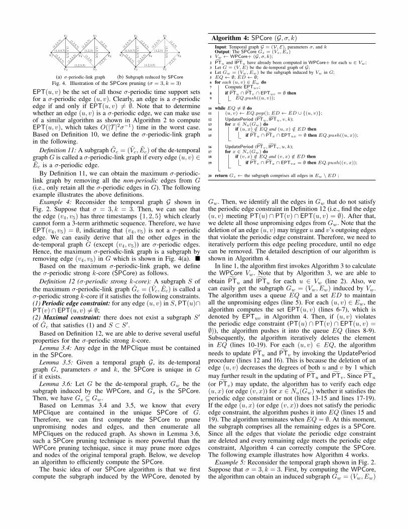
EPT(u, v) be the set of all those σ-periodic time support setsfor a σ-periodic edge (u, v). Clearly, an edge is a σ-periodicedge if and only if EPT(u, v) 6= ∅. Note that to determinewhether an edge (u, v) is a σ-periodic edge, we can make useof a similar algorithm as shown in Algorithm 2 to computeEPT(u, v), which takes O(|T |2σ−1) time in the worst case.Based on Definition 10, we define the σ-periodic-link graphin the following.

Definition 11: A subgraph Gc = (Vc, Ec) of the de-temporalgraph G is called a σ-periodic-link graph if every edge (u, v) ∈Ec is a σ-periodic edge.

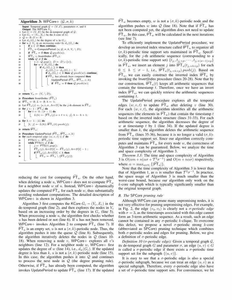
By Definition 11, we can obtain the maximum σ-periodic-link graph by removing all the non-periodic edges from G(i.e., only retain all the σ-periodic edges in G). The followingexample illustrates the above definitions.

Example 4: Reconsider the temporal graph G shown inFig. 2. Suppose that σ = 3, k = 3. Then, we can see thatthe edge (v4, v5) has three timestamps {1, 2, 5} which clearlycannot form a 3-term arithmetic sequence. Therefore, we haveEPT(v4, v5) = ∅, indicating that (v4, v5) is not a σ-periodicedge. We can easily derive that all the other edges in thede-temporal graph G (except (v4, v5)) are σ-periodic edges.Hence, the maximum σ-periodic-link graph is a subgraph byremoving edge (v4, v5) in G which is shown in Fig. 4(a). �

Based on the maximum σ-periodic-link graph, we definethe σ-periodic strong k-core (SPCore) as follows.

Definition 12 (σ-periodic strong k-core): A subgraph S ofthe maximum σ-periodic-link graph Gc = (Vc, Ec) is called aσ-periodic strong k-core if it satisfies the following constraints.(1) Periodic edge constraint: for any edge (u, v) in S, PT(u)∩PT(v) ∩ EPT(u, v) 6= ∅;(2) Maximal constraint: there does not exist a subgraph S′

of Gc that satisfies (1) and S ⊂ S′.Based on Definition 12, we are able to derive several useful

properties for the σ-periodic strong k-core.Lemma 3.4: Any edge in the MPClique must be contained

in the SPCore.Lemma 3.5: Given a temporal graph G, its de-temporal

graph G, parameters σ and k, the SPCore is unique in Gif it exists.

Lemma 3.6: Let G be the de-temporal graph, Gw be thesubgraph induced by the WPCore, and Gs is the SPCore.Then, we have Gs ⊆ Gw.

Based on Lemmas 3.4 and 3.5, we know that everyMPClique are contained in the unique SPCore of G.Therefore, we can first compute the SPCore to pruneunpromising nodes and edges, and then enumerate allMPCliques on the reduced graph. As shown in Lemma 3.6,such a SPCore pruning technique is more powerful than theWPCore pruning technique, since it may prune more edgesand nodes of the original temporal graph. Below, we developan algorithm to efficiently compute the SPCore.

The basic idea of our SPCore algorithm is that we firstcompute the subgraph induced by the WPCore, denoted by

Algorithm 4: SPCore (G, σ, k)Input: Temporal graph G = (V, E), parameters σ, and kOutput: The SPCore Gs = (Vs, Es)

1 Vw ← WPCore+ (G, σ, k);2 PTu and IPTu have already been computed in WPCore+ for each u ∈ Vw ;3 Let G = (V,E) be the de-temporal graph of G;4 Let Gw = (Vw, Ew) be the subgraph induced by Vw in G;5 EQ← ∅; ED ← ∅;6 for each (u, v) ∈ Ew do7 Compute EPTuv ;8 if PTu ∩ PTv ∩ EPTuv = ∅ then9 EQ.push((u, v));

10 while EQ 6= ∅ do11 (u, v)← EQ.pop(); ED ← ED ∪ {(u, v)};12 UpdatePeriod (PTu, IPTu, v, k);13 for x ∈ Nu(Gw) do14 if (u, x) /∈ EQ and (u, x) /∈ ED then15 if PTu ∩ PTx ∩ EPTux = ∅ then EQ.push((u, x));

16 UpdatePeriod (PTv, IPTv, u, k);17 for x ∈ Nv(Gw) do18 if (v, x) /∈ EQ and (v, x) /∈ ED then19 if PTv ∩ PTx ∩ EPTvx = ∅ then EQ.push((v, x));

20 return Gs ← the subgraph comprises all edges in Ew \ ED ;

Gw. Then, we identify all the edges in Gw that do not satisfythe periodic edge constraint in Definition 12 (i.e., find the edge(u, v) meeting PT(u) ∩ PT(v) ∩ EPT(u, v) = ∅). After that,we delete all those unpromising edges from Gw. Note that thedeletion of an edge (u, v) may trigger u and v’s outgoing edgesthat violate the periodic edge constraint. Therefore, we need toiteratively perform this edge peeling procedure, until no edgecan be removed. The detailed description of our algorithm isshown in Algorithm 4.

In line 1, the algorithm first invokes Algorithm 3 to calculatethe WPCore Vw. Note that by Algorithm 3, we are able toobtain PTu and IPTu for each u ∈ Vw (line 2). Also, wecan easily get the subgraph Gw = (Vw, Ew) induced by Vw.The algorithm uses a queue EQ and a set ED to maintainall the unpromising edges (line 5). For each (u, v) ∈ Ew, thealgorithm computes the set EPT(u, v) (lines 6-7), which isdenoted by EPTuv in Algorithm 4. Then, if (u, v) violatesthe periodic edge constraint (PT(u) ∩ PT(v) ∩ EPT(u, v) =∅)), the algorithm pushes it into the queue EQ (lines 8-9).Subsequently, the algorithm iteratively deletes the elementin EQ (lines 10-19). For each (u, v) ∈ EQ, the algorithmneeds to update PTu and PTv by invoking the UpdatePeriodprocedure (lines 12 and 16). This is because the deletion of anedge (u, v) decreases the degrees of both u and v by 1 whichmay further result in the updating of PTu and PTv . Since PTu(or PTv) may update, the algorithm has to verify each edge(u, x) (or edge (v, x)) for x ∈ Nu(Gw) whether it satisfies theperiodic edge constraint or not (lines 13-15 and lines 17-19).If the edge (u, x) (or edge (v, x)) does not satisfy the periodicedge constraint, the algorithm pushes it into EQ (lines 15 and19). The algorithm terminates when EQ = ∅. At this moment,the subgraph comprises all the remaining edges is a SPCore.Since all the edges that violate the periodic edge constraintare deleted and every remaining edge meets the periodic edgeconstraint, Algorithm 4 can correctly compute the SPCore.The following example illustrates how Algorithm 4 works.

Example 5: Reconsider the temporal graph shown in Fig. 2.Suppose that σ = 3, k = 3. First, by computing the WPCore,the algorithm can obtain an induced subgraph Gw = (Vw, Ew)

where Vw = {v1, · · · , v7}. Then, the algorithm calculatesEPT(u, v) for each (u, v) ∈ Ew (lines 6-7). Clearly, wehave EPT(v4, v5) = ∅, thus the algorithm pushes (v4, v5) intoEQ (lines 8-9). Also, the algorithm pushes (v3, v5) into EQ.The reason is that PTv3 = {[1, 3, 5]}, PTv5 = {[1, 2, 3]},and EPT(v3, v5) = {[1, 2, 3]}, and thus PTv3 ∩ PTv5 ∩EPT(v3, v5) = ∅ (lines 8-9). Subsequently, the algorithm pops(v4, v5) from EQ and updates PTv4 and PTv5 . Since PTv4and PTv5 do not change after deleting (v4, v5), the algorithmcontinues to pop (v3, v5) from EQ. After removing (v3, v5),PTv5 is updated to be an empty set. Thus, the algorithm willpushes (v5, v6) and (v5, v7) into EQ, and then iterativelyprocesses these two edges. When the algorithm terminates,we can obtain the SPCore as shown in Fig. 4(b) (the subgraphinduced by the nodes {v1, · · · , v4}). Compared to the WPCorepruning, the SPCore pruning can prune many additional nodesand edges, indicating that the SPCore pruning is indeed muchmore powerful than the WPCore pruning. �

Below, we analyze the complexity of Algorithm 4.Theorem 3.4: The time and space complexity of Algorithm

4 is O(m|T |2σ−1) and O(m+ n+ |T |2) respectively.Note that since our algorithm only works on the WPCore

(not the original temporal graph), the time cost of Algorithm4 is much less than the worst case bound in practice, whichis also confirmed in our experiments.

IV. ENUMERATION OF MPCliques

Recall that the MPClique enumeration problem is NP-hard.Thus, there does not exist a polynomial-time algorithm to solveour problem unless P=NP. Moreover, most existing maximalclique enumeration algorithms (e.g., the classic Bron-Kerboschalgorithm [10]) can only work on static graphs, it is not clearhow to apply them to identify periodic cliques in temporalgraphs. To circumvent this problem, we propose a new Bron-Kerbosch style enumeration algorithm, called MPC, whichcan efficiently compute the complete set of all MPCliques.The MPC algorithm first invokes Algorithm 4 to significantlyreduce the size of the original temporal graph. Then, theMPC algorithm transforms the reduced temporal graph intoa special static graph G, and performs a Bron-Kerbosch styleenumeration algorithm to find all maximal cliques on G. Weshow that the complete set of all maximal cliques in G is acomplete set of all MPCliques in the original temporal graphG. The detail of the MPC algorithm is shown as follows.

A. The MPC algorithmNote that the key step in MPC is to construct the trans-

formed graph G. Below, we present our graph transformationapproach.Constructing the transformed graph. Recall that in thereduced graph Gs = (Vs, Es), each node u has a set of(σ, k)-periodic time support sets, i.e., PT(u), and each edge(u, v) also has a set of σ-periodic time support sets, i.e.,EPT(u, v). Since every node u and every edge (u, v) in aMPClique C shares at least one periodic time support set, wecan decompose a MPClique into a set of nodes and edgeswhich are associated with the same periodic time supportsets. This motivate us to construct a graph G = (V , E) asfollows. For each node v ∈ Vs and an element PTsv in PT(v),we construct a vertex (v,PTsv) for V . As a result, for eachnode v ∈ Vs, we can obtain |PT(v)| vertices in V . For any

v4v2

v1

v3

ω1 : v1 {1, 3, 5}

ω2 : v1 {3, 5, 7} {1

,3, 5

,7}

{1,3,5,7}

ω5 : v3 {1, 3, 5}

ω6 : v4 {1, 3, 5}

ω3 : v2 {1, 3, 5}

ω4 : v2 {3, 5, 7}

(a) Transformed nodes

ω1

ω3

ω5

ω6

ω2

ω4

(b) Transformed graph GFig. 5. Illustration of the graph transformation method

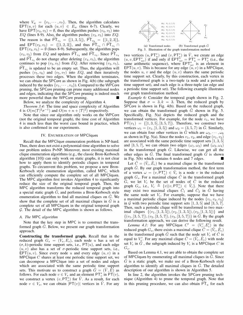
two vertices (u,PTsu) and (v,PTsv) in V , we create an edge(u, v,EPTsuv) if and only if EPTsuv = PTsu = PTsv (i.e., thesame arithmetic sequence), where EPTsuv is an element inEPT(u, v). This is because for any edge (u, v) in a MPClique,the nodes u, v and the edge (u, v) shares the same periodictime support set. Clearly, by this construction, each vertex inthe transformed graph is a two-tuple (a node and a periodictime support set), and each edge is a three-tuple (an edge anda periodic time support set). The following example illustratesour graph transformation method.

Example 6: Consider the temporal graph shown in Fig. 2.Suppose that σ = 3, k = 3. Then, the reduced graph bySPCore is shown in Fig. 4(b). Based on the reduced graph,we can obtain the transformed graph G shown in Fig. 5.Specifically, Fig. 5(a) depicts the reduced graph and thetransformed vertices. For example, for the node v1, we havePT(v1) = {[1, 3, 5], [3, 5, 7]}. Therefore, we construct twovertices ω1 = (v1, [1, 3, 5]) and ω2 = (3, 5, 7) in G. Similarly,we can obtain four other vertices in G which are ω3, · · · , ω6

as shown in Fig. 5(a). Since the nodes v1, v2, and edge (v1, v2)are associated with the same periodic time support sets [1, 3, 5]and [3, 5, 7], we can obtain two edges (ω1, ω3) and (ω2, ω4)in the transformed graph G. Likewise, we can get all theother edges in G. The final transformed graph G is shownin Fig. 5(b) which contains 6 nodes and 7 edges. �

Let C = (Vc, Ec) be a maximal clique in the transformedgraph G. By our graph transformation method, the first termof a vertex ω = (v,PTsv) ∈ Vc is a node v in the reducedgraph Gs. For a maximal clique C in the transformed graphG, we let Vc be the set of nodes of C in the reducedgraph Gs, i.e., Vc , {v|(v,PTsv) ∈ Vc}. Note that theremay exist two maximal cliques C1 and C2 in G havingthe same node set Vc. For example, suppose that we havea maximal periodic clique induced by the nodes {v1, v2, v3}in G with two periodic time support sets [1, 3, 5] and [3, 5, 7].Then, such a periodic clique will be transformed to two max-imal cliques {(v1, [1, 3, 5]), (v2, [1, 3, 5]), (v3, [1, 3, 5])} and{(v1, [3, 5, 7]), (v2, [3, 5, 7]), (v3, [3, 5, 7])} in G. By the graphtransformation approach, we can derive the following result.

Lemma 4.1: For any MPClique C ′ = (V ′c , E′c) in the

reduced graph Gs, there exists a maximal clique C = (Vc, Ec)in the transformed graph G such that the node set Vc of C isequal to V ′c . For any maximal clique C = (Vc, Ec) with nodeset Vc in G , the subgraph induced by Vc is a MPClique C inGs.

Based on Lemma 4.1, we are able to obtain the complete setof MPCliques by enumerating all maximal cliques in G. SinceG is a static graph, we make use of a Bron-Kerbosch stylealgorithm to identify all maximal cliques in G. The detaileddescription of our algorithm is shown in Algorithm 5.

In line 2, the algorithm invokes the SPCore pruning tech-nique (Algorithm 4) to prune the temporal graph. Note thatin this pruning procedure, we can also obtain PTu for each

Algorithm 5: MPC (G, σ, k)Input: Temporal graph G = (V, E), parameters σ and kOutput: the set of MPCliques C

1 C ← ∅;2 Gs = (Vs, Es)← SPCore(G, σ, k);3 PTu has been computed in SPCore for each u ∈ Vs;4 EPTuv has been calculated in SPCore for each (u, v) ∈ Es;5 G = (V , E)← construct the transformed graph based on PTu and EPTuv ;6 EnumMPClique (V , ∅, ∅, k);

7 Procedure EnumMPClique (P , R, X, k)8 if |P |+ |R| < k then return;9 if P ∪ X = ∅ then C ← C ∪ {R};

10 (v′, PTs

v′ )← arg max(v,PT

sv)∈P∪X

|P ∩N(v,PT

sv)

(G)|;

11 for (v, PTs

v) ∈ P \N(v′,PTsv′ )

(G) do

12 R′ ← R′ ∪ (v, PTs

v);13 P ′ ← P ∩N

(v,PTsv)

(G); X′ ← X ∩N(v,PT

sv)

(G);

14 EnumMPClique (P ′, R′, X′, k);15 P ← P \ (v, PTsv); X ← X ∪ (v, PT

s

v);

u ∈ Vs and EPTuv for each (u, v) ∈ Es (lines 3-4). Based onPTu and EPTuv , the algorithm can construct the transformedgraph G (line 5). Then, the algorithm performs a Bron-Kerbosch algorithm with pivoting technique to identify allmaximal cliques in G (line 6). Specifically, the set R denotesthe current clique, P denotes the set of candidate vertices, andX denotes the set of vertices that have already been processed.Note that each vertex in P , R, and X is a two-tuple (v, PT

s

v).In line 10, the algorithm adopts a similar pivoting techniquedeveloped in [12] to speed up the enumeration procedure. Notethat the operator N

(v,PTs

v)(G) is to take the neighbors of the

vertex (v, PTs

v) in the transformed graph G. The correctnessof Algorithm 5 can be guaranteed by [12] and Lemma 4.1.

B. Number of MPCliquesIn this subsection, we analyze the number of MPCliques in

the temporal graph G based on a novel concept of σ-periodicdegeneracy. The classic degeneracy is a well-known metricfor measuring the sparsity of a static graph [8]. Many real-lifenetworks are often very sparse, thus having a small degeneracy[8]. Below, we give the definition of degeneracy.

Definition 13 (Degeneracy): The degeneracy of a staticgraph G is the minimum integer δ such that each subgraphS of G contains a node v with degree no larger than δ.

Eppstein et al. [8] proved that the number of maximalcliques in a static graph is bounded by (|V | − δ)3δ/3.They also developed an efficient maximal clique enumerationalgorithm with time complexity O(δ|V |3δ/3) based on thedegeneracy ordering. The classic degeneracy, however, cannotbe directly used to bound the number of MPCliques intemporal graphs. Below, we introduce a novel concept, calledσ-periodic degeneracy, which will be applied to bound thenumber of MPCliques.

Definition 14 (σ-periodic degeneracy): Given a temporalgraph G and parameter σ, the σ-periodic degeneracy of G is thesmallest integer δ such that every σ-periodic subgraph containsa node with degree at most δ.

Since the degeneracy-based bound for the number of max-imal cliques is tailored for static graph [8], it is not clearhow to use the σ-periodic degeneracy to bound the number ofMPCliques in temporal graph. To circumvent this problem,we resort to bound the number of maximal cliques in the

transformed graph G. The rationale is that the number ofmaximal cliques in G is no less than the number of MPCliquesin the temporal graph G by Lemma 4.1. Since the transformedgraph G is a static graph, we are capable of applying theresults developed by Eppstein et al. [8] to bound the numberof maximal cliques in G. Let δ be the degeneracy of thetransformed graph G. Then, the following lemma shows thatδ is bounded by δ.

Lemma 4.2: For any temporal graph G and the transformedgraph G of the SPCore of G, we have δ ≤ δ.

Based on Lemma 4.2, we can leverage δ to bound thenumber of MPCliques in G as shown in the following theorem.

Theorem 4.1: Given a temporal graph G, parameters σ andk, the number of maximal σ-periodic k-cliques (MPCliques)in G is less than (4m2k−2σ−1 − δ)3δ/3.

Based on the results developed by Eppstein et al. [8], we canalso bound the worst-case time complexity of the MPCliqueenumeration problem by the σ-periodic degeneracy of G, i.e.,δ. Specifically, we have the following results.

Theorem 4.2: Given a temporal graph G, parameters σ andk, there exists an algorithm to enumerate all MPCliques inG in O(δm2k−2σ−13δ/3) time, where δ is the σ-periodicdegeneracy of G and m is the number of temporal edges in G.

Not that Theorem 4.2 indicates that enumerating allMPCliques in a temporal graph G is fixed-parameter tractablewith respect to the parameter σ-periodic degeneracy δ of G.Since the σ-periodic degeneracy of G is typically very smallin real-life temporal graphs, the proposed algorithm can bevery efficient in practice.

V. EXPERIMENTS

In our experiments, we implement four various algorithmsto identify maximal σ-periodic k-cliques: MPC-B, MPC-KC,MPC-WC+, MPC-SC. Specifically, MPC-B is a baselinealgorithm which is not integrated with any graph reductiontechniques. MPC-B first computes PT(u) (for each node u)and EPT(u, v) (for each edge (u, v)) using Algorithm 2, andthen constructs a transformed graph G. After that, MPC-Buses the Bron-Kerbosch algorithm with a pivoting technique toenumerate all maximal σ-periodic k-cliques on G. MPC-KCis the MPC-B algorithm combined with the KCore pruningrule. MPC-WC+ denotes the MPC-B algorithm integrated withthe WPCore pruning rule. Note that we also implement twoalgorithms which are WC (Algorithm 1) and WC+ to computethe WPCore. The MPC-WC+ algorithm is integrated with amore efficient WC+ algorithm. MPC-SC denotes the MPC-Balgorithm with the SPCore pruning rule, i.e., Algorithm 5. Toevaluate the effectiveness of the proposed maximal σ-periodick-clique model, we use WPCore and SPCore as two intuitivebaseline models. The reasons are as follows. First, to thebest of our knowledge, there is no existing community modelthat can be used to model periodic communities in temporalnetworks. Second, by Definitions 9 and 12, both WPCoreand SPCore can capture periodic and cohesive properties of acommunity in temporal graphs, thus WPCore and SPCore canserve as two baselines for modeling periodic communities. Allalgorithms are implemented in Python. All the experiments areconducted on a server of Linux kernel 4.4 with Intel Core(TM)i5-8400@3.20GHz and 32 GB main memory.Datasets. We use five different types of real-life temporalnetworks in the experiments. The detailed statistics of our

��102

103

����������� ���

�� 2231

890

310

161

�102

103

����������� ���

�� 2314

768545

326

���102

103

104

����������� ���� 12987

3765

416

147

�����101

102

103

����������� ���� 3476

1154

187

61

���

102

103

104

105

����������� ���� >2days

7421

1056415

MPC-B MPC-KC MPC-WC+ MPC-SC

Fig. 7. Running time of different algorithms on various datasets (σ = 4, k = 4)

TABLE IIRUNNING TIME OF DIFFERENT ALGORITHMS WITH VARYING PARAMETERS (DBLP)

σ = 3 σ = 4 σ = 5 σ = 6 σ = 7MPC-KCMPC-WC+ MPC-SC MPC-KCMPC-WC+ MPC-SC MPC-KCMPC-WC+ MPC-SC MPC-KCMPC-WC+ MPC-SC MPC-KCMPC-WC+ MPC-SC

k = 3 INF 32,213 4,339 24,517 12,313 1,237 8,321 4,567 936 4,235 3,456 804 2,145 1,023 144k = 4 23,100 3,574 580 7,421 1,056 415 3,441 774 326 1,960 114 71 1,467 48 38k = 5 9,770 736 280 3,428 801 75 1,771 417 45 1,220 63 35 1,023 33 37k = 6 4,464 621 112 2,035 585 45 1,643 142 32 980 32 27 576 14 16k = 7 2,382 534 24 1,292 51 23 1,201 44 27 620 21 20 231 10 11

TABLE IDATASETS

Dataset |V | |E| |E| dmax |T | Time scaleHS 327 5,818 20,448 322 101 hourPS 242 8,317 26,351 393 34 hour

LKML 26,885 159,996 328,092 14,172 96 monthEnron 86,978 297,456 499,983 4,311 48 monthDBLP 1,729,816 8,546,306 12,007,380 5,980 59 year

HS PS LKML Enron DBLP101

102

103

104

105

����

������

����

�

WCWC+

Fig. 6. Running time of WC and WC+

datasets are summarized in Table I. In Table I, the firsttwo datasets are human contact temporal networks whichare download from (http://www.sociopatterns.org/datasets/).Specifically, HS is a temporal network of face-to-face contactsbetween students in a French high school [2], and PS isa temporal network of contacts between the children andteachers in a French primary school [2]. Each snapshot ofthese temporal networks is extracted in a hour. Both LKMLand Enron are temporal communication networks downloadedfrom (http://konect.uni-koblenz.de), where each temporal edge(u, v, t) represents an email communication from a user uto v at time t. Each snapshot of these temporal networksis extracted in a month. DBLP is a temporal collaborationnetwork of authors in DBLP downloaded from (http://dblp.uni-trier.de/xml/), where each temporal edge (u, v, t) denotesthat two authors u and v co-authored one paper at time t. Eachsnapshot of DBLP is extracted in a year. In Table I, dmax is themaximum number of temporal edges associated with a node,and |T | denotes the number of snapshots.Parameter settings. There are two parameters k, σ in ouralgorithm. For the parameter k, we vary it from 3 to 7 with adefault value of 3. We also vary σ from 3 to 7 with a defaultvalue of 3. Unless otherwise specified, the value of the otherparameter are set to its default value when varying a parameter.

A. Efficiency Testing

Exp-1: Comparison between WC and WC+. Fig. 6 evaluatesthe running time of WC (Algorithm 1) and WC+ (Algorith-m 3) for computing WPCore. As can be seen, WC+ is muchfaster than WC on all datasets. The running time of WC+is around a half of the running time of WC. For example, onEnron, WC+ takes 1.1 seconds and WC consumes 2.3 secondsto identify all MPCliques. The reason is that WC+ is basedon an on-demand computing paradigm which can substantiallyreduce redundant computations. These results are consistentwith our theoretical analysis presented in Section III-A. In thefollowing experiments, we will use WC+ to compute WPCore.

TABLE IIINUMBER OF NODES OF THE REDUCED GRAPH

KCore WPCore SPCoreHS 326 99% 280 86% 165 51%PS 242 100% 233 96% 211 87%

LKML 9,773 36% 1,785 6.6% 926 3.4%Enron 18,591 21% 3,314 3.8% 2,315 2.7%DBLP 1,258,540 73% 126,357 7.3% 73,109 4.2%

Exp-2: Efficiency of various MPClique mining algorithm-s. Fig. 7 shows the running time of MPC-B, MPC-KC,MPC-WC+ and MPC-SC on different datasets with parametersσ = 4 and k = 4. Similar results can also be observed underthe other parameter settings. From Fig. 7, we can see thatMPC-SC is much faster than all the other competitors on alldatasets. For example, on DBLP, MPC-SC takes around 7minutes to enumerate all MPCliques which cuts the runningtime over MPC-WC+ and MPC-KC by 154% and 1,688%respectively. Note that MPC-B cannot get results on DBLP in2 days. These results indicate that the SPCore pruning ruleis indeed very powerful in practice which are consistent withour analysis in Section III-B.Exp-3: Effect of parameters. Table. II reports the runningtime of different algorithms with varying parameters on DBLP.Similar results can also be observed on the other datasets.Since the parameters do not significantly affect MPC-B, wefocus mainly on MPC-KC, MPC-WC+ and MPC-SC. As canbe seen, MPC-SC is faster than all the other algorithms underalmost all parameter settings. In general, the running time ofMPC-KC, MPC-WC+ and MPC-SC decrease with increasingk and σ, because the size of the transformed graph decreases ask or σ increases. Note that when σ = 7 and k ≥ 5, MPC-WC+is slightly faster than MPC-SC. The reason could be that fora large σ and k, the original temporal graph can be reducedto a very small graph by WPCore, thus the benefit of SPCoremay be not significant.Exp-4: Number of nodes of the reduced graph. Table IIIshows the number of remaining nodes obtained by KCore,WPCore and SPCore on all datasets under the default pa-rameter setting. In columns 2-4 of Table III, the left integeris the number of remaining nodes and the right value isthe percentage of the remaining nodes over all nodes in thegraph. As can be seen, both WPCore and SPCore can prunea large number of unpromising nodes on large datasets. Forexample, on DBLP, the number of remaining nodes obtainedby WPCore and SPCore is only 7.3% and 4.2% of theoriginal graph respectively. These results confirm that ourgraph reduction techniques are indeed very effective on largereal-life temporal networks.Exp-5: Size of the transformed graph. Table IV reportsthe size of the transformed graph G = (V , E) generated byMPC-SC. We can observe that the size of G scales linearly

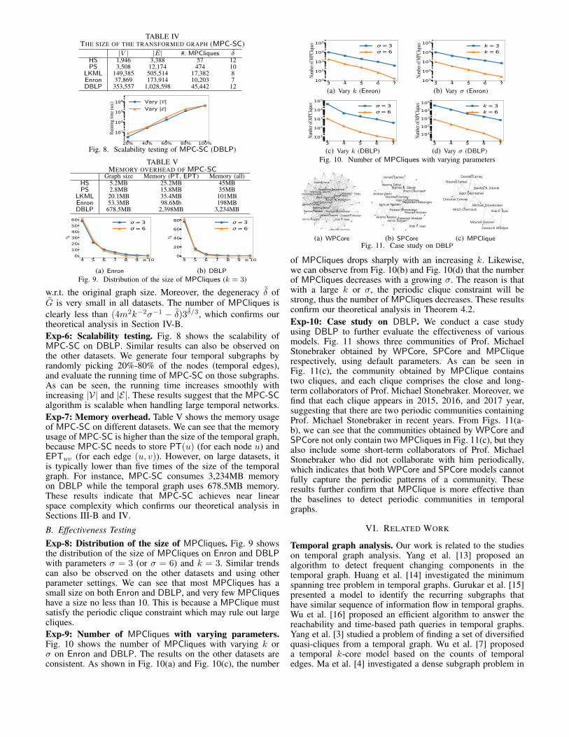
TABLE IVTHE SIZE OF THE TRANSFORMED GRAPH (MPC-SC)

|V | |E| #. MPCliques δHS 1,946 3,388 57 12PS 3,508 12,174 474 10

LKML 149,385 505,514 17,382 8Enron 37,869 173,914 10,203 7DBLP 353,557 1,028,598 45,442 12

20% 40% 60% 80% 100%

101

102

103

104

��

�������

����

� Vary ||Vary ||

Fig. 8. Scalability testing of MPC-SC (DBLP)

TABLE VMEMORY OVERHEAD OF MPC-SC

Graph size Memory (PT, EPT) Memory (all)HS 5.2MB 25.2MB 45MBPS 2.8MB 15.8MB 35MB

LKML 20.1MB 35.4MB 101MBEnron 53.3MB 98.6Mb 198MBDBLP 678.5MB 2,398MB 3,234MB

4 5 6 7 8 9 ≥100102030405060

�

σ=3σ=6

(a) Enron

4 5 6 7 8 9 ≥100

20

40

60

80

�

σ=3σ=6

(b) DBLP

Fig. 9. Distribution of the size of MPCliques (k = 3)

w.r.t. the original graph size. Moreover, the degeneracy δ ofG is very small in all datasets. The number of MPCliques isclearly less than (4m2k−2σ−1 − δ)3δ/3, which confirms ourtheoretical analysis in Section IV-B.Exp-6: Scalability testing. Fig. 8 shows the scalability ofMPC-SC on DBLP. Similar results can also be observed onthe other datasets. We generate four temporal subgraphs byrandomly picking 20%-80% of the nodes (temporal edges),and evaluate the running time of MPC-SC on those subgraphs.As can be seen, the running time increases smoothly withincreasing |V| and |E|. These results suggest that the MPC-SCalgorithm is scalable when handling large temporal networks.Exp-7: Memory overhead. Table V shows the memory usageof MPC-SC on different datasets. We can see that the memoryusage of MPC-SC is higher than the size of the temporal graph,because MPC-SC needs to store PT(u) (for each node u) andEPTuv (for each edge (u, v)). However, on large datasets, itis typically lower than five times of the size of the temporalgraph. For instance, MPC-SC consumes 3,234MB memoryon DBLP while the temporal graph uses 678.5MB memory.These results indicate that MPC-SC achieves near linearspace complexity which confirms our theoretical analysis inSections III-B and IV.

B. Effectiveness TestingExp-8: Distribution of the size of MPCliques. Fig. 9 showsthe distribution of the size of MPCliques on Enron and DBLPwith parameters σ = 3 (or σ = 6) and k = 3. Similar trendscan also be observed on the other datasets and using otherparameter settings. We can see that most MPCliques has asmall size on both Enron and DBLP, and very few MPCliqueshave a size no less than 10. This is because a MPClique mustsatisfy the periodic clique constraint which may rule out largecliques.Exp-9: Number of MPCliques with varying parameters.Fig. 10 shows the number of MPCliques with varying k orσ on Enron and DBLP. The results on the other datasets areconsistent. As shown in Fig. 10(a) and Fig. 10(c), the number

3 4 5 6 7101

102

103

104

105

���

� ����

����

���� σ=3

σ=6

(a) Vary k (Enron)3 4 5 6 7101

102

103

104

105

���

� ����

����

���� k=3

k=6

(b) Vary σ (Enron)

3 4 5 6 7101

102

103

104

105

���

� ����

����

���� σ=3

σ=6

(c) Vary k (DBLP)3 4 5 6 7

101102103104105

���

� ����

����

���� k=3

k=6

(d) Vary σ (DBLP)Fig. 10. Number of MPCliques with varying parameters

Magdalena Balazinska

Mitch Cherniack

Samuel Madden

Joseph M. Hellerstein

Stanley B. Zdonik

Ugur Çetintemel

Nesime Tatbul

Donald Carney

Christian Convey

Andrew Pavlo

Jeremy Kepner

Jennie Duggan

Michael Stonebraker

Michael J. CareyDavid Maier

Ihab F. Ilyas

Mourad Ouzzani

Ziawasch Abedjan

(a) WPCore

Magdalena Balazinska

Mitch Cherniack

Samuel Madden

Stanley B. Zdonik

Ugur Çetintemel

Nesime Tatbul

Donald Carney

Christian ConveyAndrew Pavlo

Jeremy Kepner

Jennie Duggan

Michael Stonebraker

Ihab F. Ilyas

Mourad Ouzzani

Ziawasch Abedjan

(b) SPCore (c) MPCliqueFig. 11. Case study on DBLP

of MPCliques drops sharply with an increasing k. Likewise,we can observe from Fig. 10(b) and Fig. 10(d) that the numberof MPCliques decreases with a growing σ. The reason is thatwith a large k or σ, the periodic clique constraint will bestrong, thus the number of MPCliques decreases. These resultsconfirm our theoretical analysis in Theorem 4.2.Exp-10: Case study on DBLP. We conduct a case studyusing DBLP to further evaluate the effectiveness of variousmodels. Fig. 11 shows three communities of Prof. MichaelStonebraker obtained by WPCore, SPCore and MPCliquerespectively, using default parameters. As can be seen inFig. 11(c), the community obtained by MPClique containstwo cliques, and each clique comprises the close and long-term collaborators of Prof. Michael Stonebraker. Moreover, wefind that each clique appears in 2015, 2016, and 2017 year,suggesting that there are two periodic communities containingProf. Michael Stonebraker in recent years. From Figs. 11(a-b), we can see that the communities obtained by WPCore andSPCore not only contain two MPCliques in Fig. 11(c), but theyalso include some short-term collaborators of Prof. MichaelStonebraker who did not collaborate with him periodically,which indicates that both WPCore and SPCore models cannotfully capture the periodic patterns of a community. Theseresults further confirm that MPClique is more effective thanthe baselines to detect periodic communities in temporalgraphs.

VI. RELATED WORK

Temporal graph analysis. Our work is related to the studieson temporal graph analysis. Yang et al. [13] proposed analgorithm to detect frequent changing components in thetemporal graph. Huang et al. [14] investigated the minimumspanning tree problem in temporal graphs. Gurukar et al. [15]presented a model to identify the recurring subgraphs thathave similar sequence of information flow in temporal graphs.Wu et al. [16] proposed an efficient algorithm to answer thereachability and time-based path queries in temporal graphs.Yang et al. [3] studied a problem of finding a set of diversifiedquasi-cliques from a temporal graph. Wu et al. [7] proposeda temporal k-core model based on the counts of temporaledges. Ma et al. [4] investigated a dense subgraph problem in

temporal graphs. Li et al. [5] developed an efficient algorithmto identify persistent communities in temporal graphs. To thebest of our knowledge, our work is the first to study theproblem of mining periodic communities in temporal graphs.Community detection in dynamic graphs. There is a numberof studies for mining communities on dynamic networks [17].Most of them aim to identify and analyze the communitystructures that evolve over time. Lin et al. [18] proposed aprobabilistic generative model to analyze evolving commu-nities. Chen et al. [19] developed an algorithm for trackingcommunity dynamics. Agarwal et al. [20] studied how tofind dense clusters for dynamic microblog streams. Li et al.[21] devised an algorithm to maintain the k-core in largedynamic graphs. Rossetti et al. [22] proposed an onlineiterative algorithm for tracking the evolution of communities.Unlike these studies, our work focuses mainly on detectingperiodic communities in temporal graphs.Maximal cliques enumeration. Our work is also related tothe maximal clique enumeration problem. Notable algorithmsfor enumerating maximal clique include the classic Bron-Kerbosch algorithm [10] and its variants [8], [12], [23]. Tomitaet al. [12] proved that the Bron-Kerbosch algorithm witha pivoting technique is essentially optimal according to theworst-case bound. Eppstein et al. [8] developed an algorithmwhich is fixed-parameter tractable w.r.t. the degeneracy of thegraph. Cheng et al. [23] proposed an external-memory algo-rithm for clique enumeration in massive graphs. More recently,Himmel [24] developed a Bron-Kerbosch style algorithm forenumerating maximal cliques in temporal graph. Their work,however, cannot be used to enumerate periodic cliques.Periodic behavior mining. The studies of periodic behaviormining are also related to our work. Notable examples aresummarized below. Li et al. [25] addressed the problem ofmining periodic behaviors for moving objects. Kurashima etal. [26] modeled the periodic actions in real-world (e.g., eating,sleep, and exercise) to make predictions for future actions.Radinsky et al. [27] also developed a temporal model topredict the periodic actions. Lahiri et al. [28] investigateda problem of mining periodic subgraphs in dynamic socialnetworks. Their work, however, does not consider the com-munities in the periodic subgraphs, thus cannot be used formining periodic communities.

VII. CONCLUSION

In this work, we study a problem of mining periodiccommunities in temporal graph. We propose a novel model,called maximal σ-periodic k-clique, to characterize the peri-odic communities in a temporal graph. To find all maximalσ-periodic k-cliques, we first develop several new pruningtechniques to substantially reduce the size of the temporalgraph. Then, on the reduced temporal graph, we propose anenumeration algorithm based on a carefully-designed graphtransformation technique to efficiently identify all maximal σ-periodic k-cliques. Comprehensive experiments on five real-life temporal networks demonstrate the efficiency, scalabilityand effectiveness of our algorithms.Acknowledgement. This work was partially supported by (i) NS-FC Grants 61772346, 61732003, U1809206, 61572119, 61622202,U1401256, 61729201; (ii) National Key R&D Program of China2018YFB1004402; (iii) Beijing Institute of Technology ResearchFund Program for Young Scholars; (iv) ARC Discovery Project GrantDP160101513; (v) Fundamental Research Funds for the Central

Universities N150402005. Guoren Wang is the corresponding authorof this paper.

REFERENCES

[1] P. Vanhems, A. Barrat, C. Cattuto, J.-F. Pinton, N. Khanafer, C. Regis,B. a Kim, B. Comte, and N. Voirin, “Estimating potential infectiontransmission routes in hospital wards using wearable proximity sensors,”PLoS ONE, vol. 8, p. e73970, 2013.

[2] J. Fournet and A. Barrat, “Contact patterns among high school students,”PLOS ONE, vol. 9, p. e107878, 2014.

[3] Y. Yang, D. Yan, H. Wu, J. Cheng, S. Zhou, and J. C. S. Lui, “Diversifiedtemporal subgraph pattern mining,” in KDD, 2016.

[4] S. Ma, R. Hu, L. Wang, X. Lin, and J. Huai, “Fast computation of densetemporal subgraphs,” in ICDE, 2017.

[5] R.-H. Li, J. Su, L. Qin, J. X. Yu, and Q. Dai, “Persistent communitysearch in temporal networks,” in ICDE, 2018.

[6] I. R.Fischhoff, S. R.Sundaresan, J. Cordingley, H. M.Larkin, and M.-J.Sellier, “Social relationships and reproductive state influence leadershiproles in movements of plains zebra, equus burchellii,” Animal Behaviour,vol. 73, no. 5, pp. 825–831, 2007.

[7] H. Wu, J. Cheng, Y. Lu, Y. Ke, Y. Huang, D. Yan, and H. Wu,“Core decomposition in large temporal graphs,” in IEEE InternationalConference on Big Data, 2015.

[8] D. Eppstein, M. Loffler, and D. Strash, “Listing all maximal cliquesin large sparse real-world graphs,” ACM Journal of ExperimentalAlgorithmics, vol. 18, 2013.

[9] V. Batagelj and M. Zaversnik, “An O(m) algorithm for cores decompo-sition of networks,” CoRR cs.DS/0310049, 2003.

[10] C. Bron and J. Kerbosch, “Algorithm 457: finding all cliques of anundirected graph,” Communications of the ACM, vol. 16, no. 9, pp.575–577, 1973.

[11] S. B. Seidman, “Network structure and minimum degree,” Socialnetworks, vol. 5, no. 3, pp. 269–287, 1983.

[12] E. Tomita, A. Tanaka, and H. Takahashi, “The worst-case timecomplexity for generating all maximal cliques and computationalexperiments,” Theoretical Computer Science, vol. 363, no. 1, pp. 28–42,2006.

[13] Y. Yang, J. X. Yu, H. Gao, J. Pei, and J. Li, “Mining most frequentlychanging component in evolving graphs,” World Wide Web, vol. 17,no. 3, pp. 351–376, 2014.

[14] S. Huang, A. W. Fu, and R. Liu, “Minimum spanning trees in temporalgraphs,” in SIGMOD, 2015.

[15] S. Gurukar, S. Ranu, and B. Ravindran, “COMMIT: A scalable approachto mining communication motifs from dynamic networks,” in SIGMOD,2015.

[16] H. Wu, Y. Huang, J. Cheng, J. Li, and Y. Ke, “Reachability and time-based path queries in temporal graphs,” in ICDE, 2016.

[17] G. Rossetti and R. Cazabet, “Community discovery in dynamicnetworks: A survey,” ACM Comput. Surv., vol. 51, no. 2, pp. 35:1–35:37, 2018.

[18] Y.-R. Lin, Y. Chi, S. Zhu, H. Sundaram, and B. L. Tseng, “Facetnet: Aframework for analyzing communities and their evolutions in dynamicnetworks,” in WWW, 2008.

[19] Z. Chen, K. A. Wilson, Y. Jin, W. Hendrix, and N. F. Samatova,“Detecting and tracking community dynamics in evolutionary networks,”in ICDMW, 2010.

[20] M. K. Agarwal, K. Ramamritham, and M. Bhide, “Real time discoveryof dense clusters in highly dynamic graphs: Identifying real world eventsin highly dynamic environments,” PVLDB, vol. 5, no. 10, 2012.

[21] R. H. Li, J. X. Yu, and R. Mao, “Efficient core maintenance inlarge dynamic graphs,” IEEE Transactions on Knowledge and DataEngineering, vol. 26, no. 10, pp. 2453–2465, 2014.

[22] G. Rossetti, L. Pappalardo, D. Pedreschi, and F. Giannotti, “Tiles: anonline algorithm for community discovery in dynamic social networks,”Machine Learning, vol. 106, no. 8, pp. 1213–1241, 2017.

[23] J. Cheng, Y. Ke, A. W.-C. Fu, J. X. Yu, and L. Zhu, “Finding maximalcliques in massive networks,” ACM Trans. Database Syst., vol. 36, no. 4,pp. 21:1–21:34, 2011.

[24] A.-S. Himmel, H. Molter, R. Niedermeier, and M. Sorge, “Adapting thebron–kerbosch algorithm for enumerating maximal cliques in temporalgraphs,” Social Network Analysis and Mining, vol. 7, no. 1, pp. 7–35,2017.

[25] Z. Li, B. Ding, J. Han, R. Kays, and P. Nye, “Mining periodic behaviorsfor moving objects,” in KDD, 2010.

[26] T. Kurashima, T. Althoff, and J. Leskovec, “Modeling Interdependentand Periodic Real-World Action Sequences,” in WWW, 2018.

[27] K. Radinsky, K. Svore, S. Dumais, J. Teevan, A. Bocharov, andE. Horvitz, “Modeling and predicting behavioral dynamics on the web,”in WWW, 2012.

[28] M. Lahiri and T. Y. Berger-Wolf, “Periodic subgraph mining in dynamicnetworks,” Knowledge and Information Systems, vol. 24, no. 3, pp. 467–497, 2010.