March 2005

• Discuss my ongoing work on the monetary transmission mechanism (ACEL (2005)).

– Can models with nominal rigidities generate persistent quantity responses and inertial inflation responses to monetary policy shocks for `plausible’ parameter values?

– What are the implications of these models for how the economy responds to technology shocks?

• How does the response depend on monetary policy?

• What are the key shortcomings of these models?

Structure of Talk

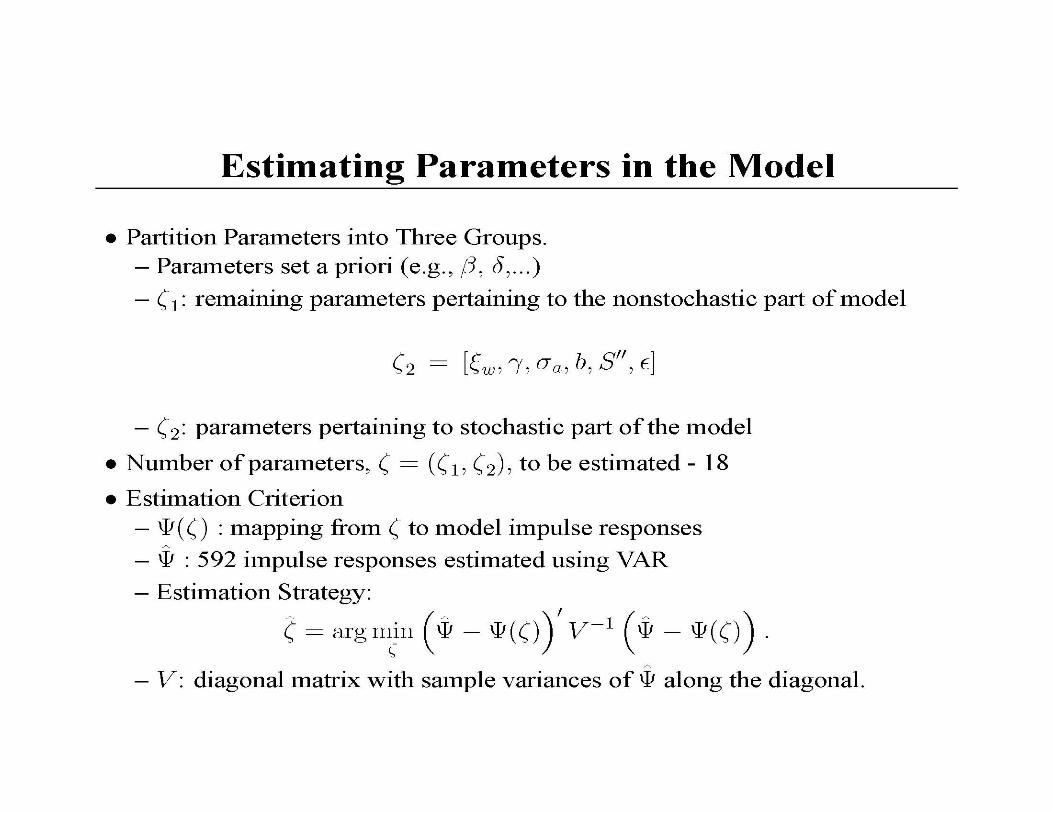
• Should we should use full information methods or limited information methods when estimating the parameters of GE models and assessing models’performance?

– Remarkably little formal work on this question.

Question

The hare strategy– Variants of full information MLE.– Fully parameterize the stochastic environment faced by agents.

– Christiano (1986), McGrattan (1989), Smets and Wouters (2004), CKM (2005).

–• The tortoise strategy

– Limited information strategy - focus on a subset of the shocks impacting on agents’ environment.

– Prescott (1986)– CEE (2004): monetary policy shocks.– Burnside, Eichenbaum and Fischer (2004): fiscal policy shocks.– Fisher (2004): capital embodied and neutral technology shocks.– ACEL (2005): policy and technology shocks.

The Tortoise and the Hare

• Hare strategy: identification is achieved by strong assumptions on the time series representation for the shocks to agents’environments.

– Parsimonious ARMA representations for things like shocks to technology, preferences and measurement error.

Identification

Identification• Tortoise strategy: achieve identification by

imposing a subset of model’s assumptions on a reduced form representation of the data.

– Estimate dynamic response function of macro variables to an identified shock.

– Choose structural parameters of model to minimize distance between this dynamic response function and response function implied by the full economic model.

• Modern macro models imply data have an ARMA representation.

– Reduced form representation used in first step of tortoise 1 strategy typically involves a finite ordered VAR.

• Is this a source of serious concern?

–No.

• If the DGP satisfies the identifying imposed on a VARs, then inference from VAR’s doesn’t lead one awry.

Possible Problem with Tortoise

CEV (2005)• Run VARs in data generated by DSGE Models.

– CKM RBC examples and ACEL.

• Long-Run Exclusion and Sign Identifying Restrictions – You would not be misled about true impulse response functions as sample

size grows.– Small samples:

• Not much bias as long as you have at least one more variable in VAR than the number of `important’ shocks.

• Perhaps there would be substantial sampling uncertainty, but theeconometrician would know it.

• Short-Run Exclusion and Sign Identifying Restrictions– No Evidence of Small or Large Sample Bias – Relatively Little Sampling Uncertainty– Robust to Which Variables are Included in VAR.

• Today I only have time to discuss ACEL based results.

Remainder of Talk

• ACEL monetary business cycle model.

• Concluding comments– The importance of understanding labor

markets for understanding the monetary transmission mechanism.

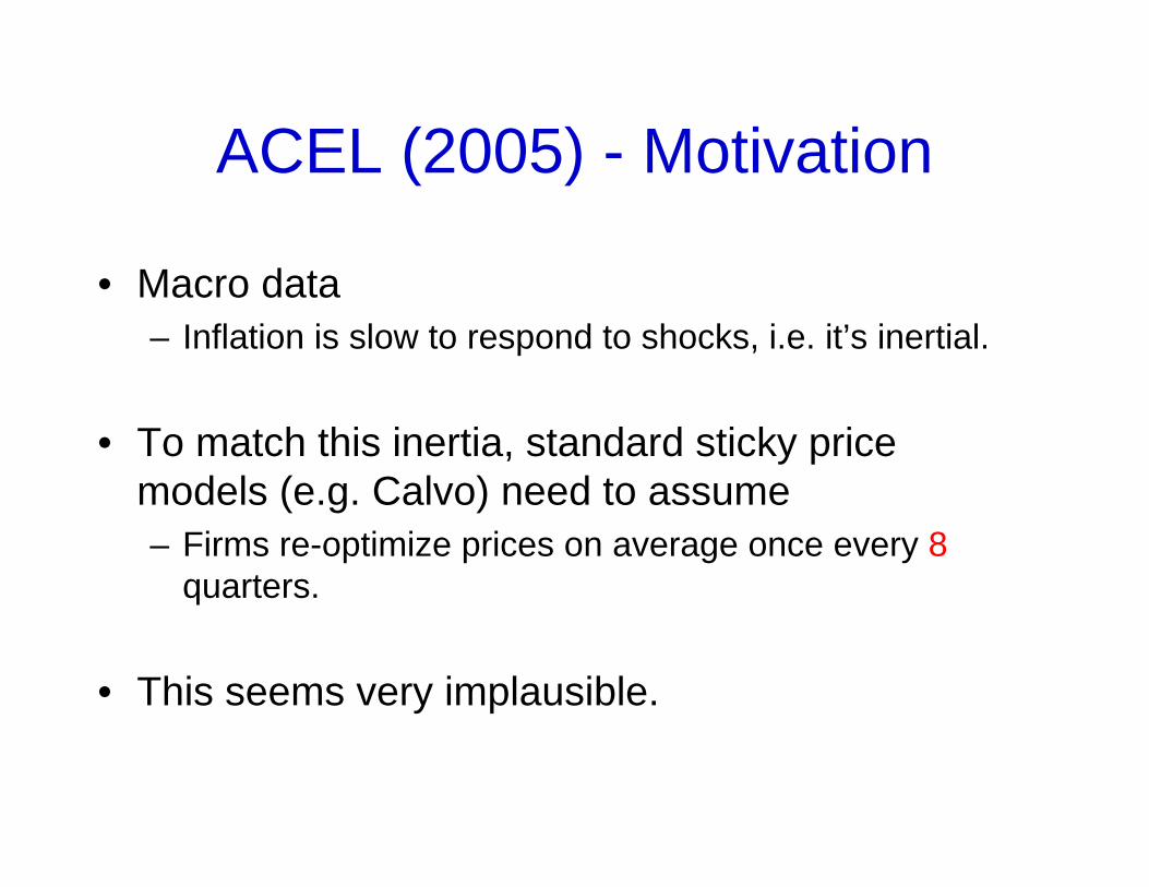
ACEL (2005) - Motivation

• Macro data– Inflation is slow to respond to shocks, i.e. it’s inertial.

• To match this inertia, standard sticky price models (e.g. Calvo) need to assume– Firms re-optimize prices on average once every 8

quarters.

• This seems very implausible.

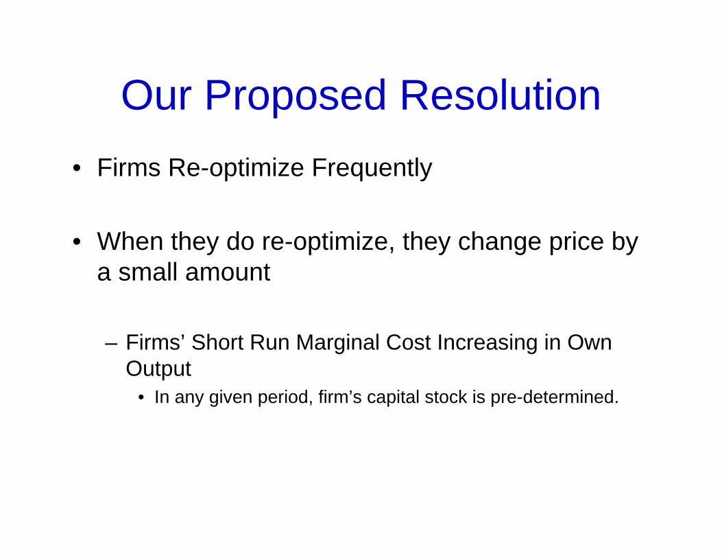
Our Proposed Resolution• Firms Re-optimize Frequently

• When they do re-optimize, they change price by a small amount

– Firms’ Short Run Marginal Cost Increasing in Own Output

• In any given period, firm’s capital stock is pre-determined.

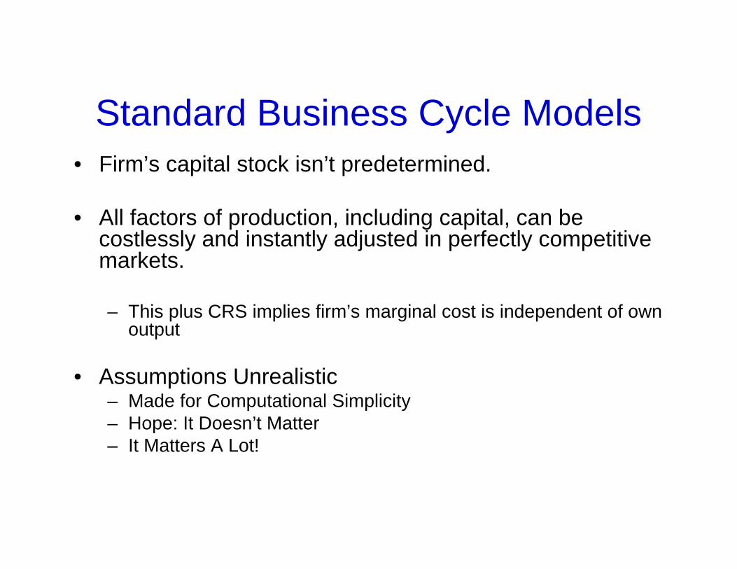
Standard Business Cycle Models• Firm’s capital stock isn’t predetermined.

• All factors of production, including capital, can be costlessly and instantly adjusted in perfectly competitive markets.

– This plus CRS implies firm’s marginal cost is independent of own output

• Assumptions Unrealistic– Made for Computational Simplicity– Hope: It Doesn’t Matter– It Matters A Lot!

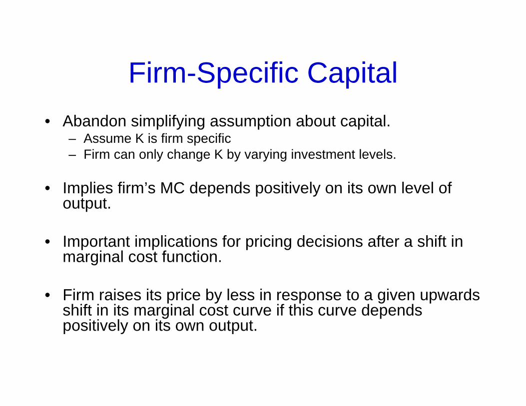
Firm-Specific Capital• Abandon simplifying assumption about capital.

– Assume K is firm specific– Firm can only change K by varying investment levels.

• Implies firm’s MC depends positively on its own level of output.

• Important implications for pricing decisions after a shift in marginal cost function.

• Firm raises its price by less in response to a given upwards shift in its marginal cost curve if this curve depends positively on its own output.

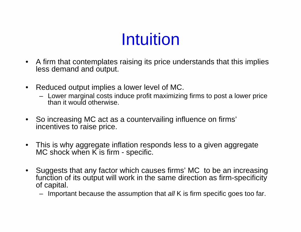
Intuition• A firm that contemplates raising its price understands that this implies

less demand and output.

• Reduced output implies a lower level of MC.– Lower marginal costs induce profit maximizing firms to post a lower price

than it would otherwise.

• So increasing MC act as a countervailing influence on firms’incentives to raise price.

• This is why aggregate inflation responds less to a given aggregate MC shock when K is firm - specific.

• Suggests that any factor which causes firms’ MC to be an increasing function of its output will work in the same direction as firm-specificity of capital.– Important because the assumption that all K is firm specific goes too far.

Intuition…

• Effect of firm specific capital quantitatively important when– Demand is Elastic– Marginal Cost Curve is Steep

• Can’t answer this question a priori– Depends on values of key model parameters.

Strategy for Evaluating Our Proposal

• Estimate Model Parameters Using Macro Data– Choose parameters of model to match impulse

response functions of 10 aggregate time series to three shocks

• Monetary Policy Shocks, Neutral and Capital Embodied Technology Shocks

– These shocks account for over 50% of cyclical fluctuations in output.

• Can we account for inflation inertia with plausible inertia in price-re-optimization?

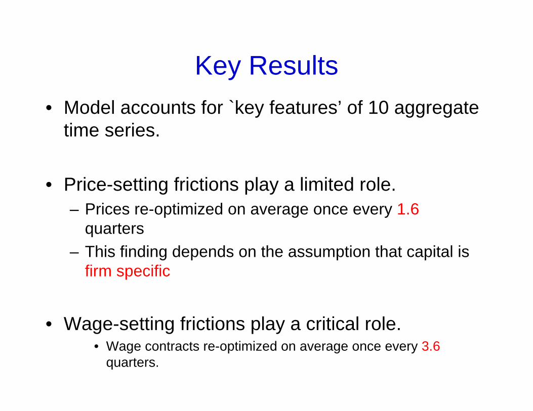
Key Results• Model accounts for `key features’ of 10 aggregate

time series.

• Price-setting frictions play a limited role. – Prices re-optimized on average once every 1.6

quarters – This finding depends on the assumption that capital is

firm specific

• Wage-setting frictions play a critical role.• Wage contracts re-optimized on average once every 3.6

quarters.

Key results…• Model does a good job of accounting for

economy’s response to our three identified shocks.

• Monetary policy shocks affect economy the way Friedman would anticipate.– Monetary policy shock has persistent real effects.

• Technology shocks affect economy the way a student of RBC models would anticipate.

– Neutral and capital embodied technology shocks drive output, investment, consumption and employment up.

But…• Monetary policy plays a key role in response of

economy to technology shocks

• Monetary policy accommodates positive neutral and capital technology shocks.

• According to our model, in absence of monetary accommodation,

– Output and hours would fall in the wake of a positive neutral technology shock;

– Output and hours worked would rise by much lessthan they actually do after a positive capital embodied technology shock.

Model: Variant of CEE (2004)

• Modified to allow for two types of technology shocks.

• Firm-Specific Capital – Capital is completely firm specific– Firms own and accumulate their capital– No capital rental markets

Brief Description of Model• Firms

• Households

• Monetary Authority

• Goods Market Clearing and Equilibrium

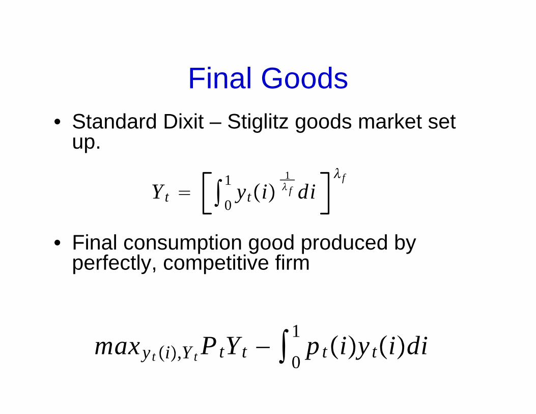
Final Goods• Standard Dixit – Stiglitz goods market set

up.

• Final consumption good produced by perfectly, competitive firm

Yt 0

1 yti1 f di

f

maxyt i,Y t PtYt − 01

ptiytidi

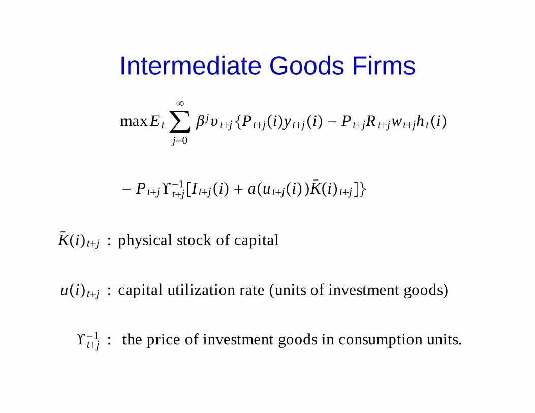
Intermediate Goods Firms

maxE t∑j0

j tjPtjiytji − PtjR tjwtjh ti

− Ptj tj−1 I tji autjiKi tj

Kitj : physical stock of capital

uitj : capital utilization rate (units of investment goods)

tj−1 : the price of investment goods in consumption units.

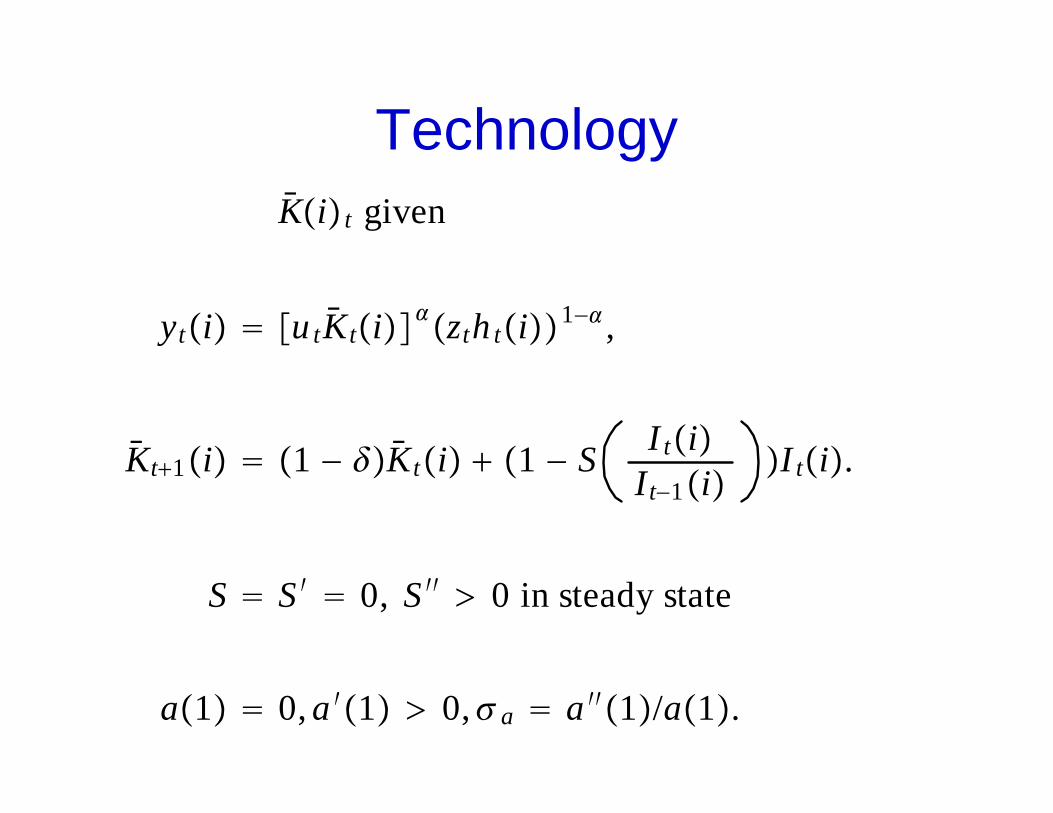
TechnologyKi t given

yti utKtizth ti1− ,

Kt1i 1 − Kti 1 − S I tiIt−1i

I ti.

S S ′ 0, S ′′ 0 in steady state

a1 0, a ′1 0, a a ′′1/a1.

Technology…

• Firms own their capital which can’t be adjusted during the period

– Can only be changed by varying the rate of investment over time.

• Price of investment goods relative to consumption goods is

• Equilibrium outcome in environment where agents transform output of final goods producers into investment goods using a linear technology with slope

tj−1

tj

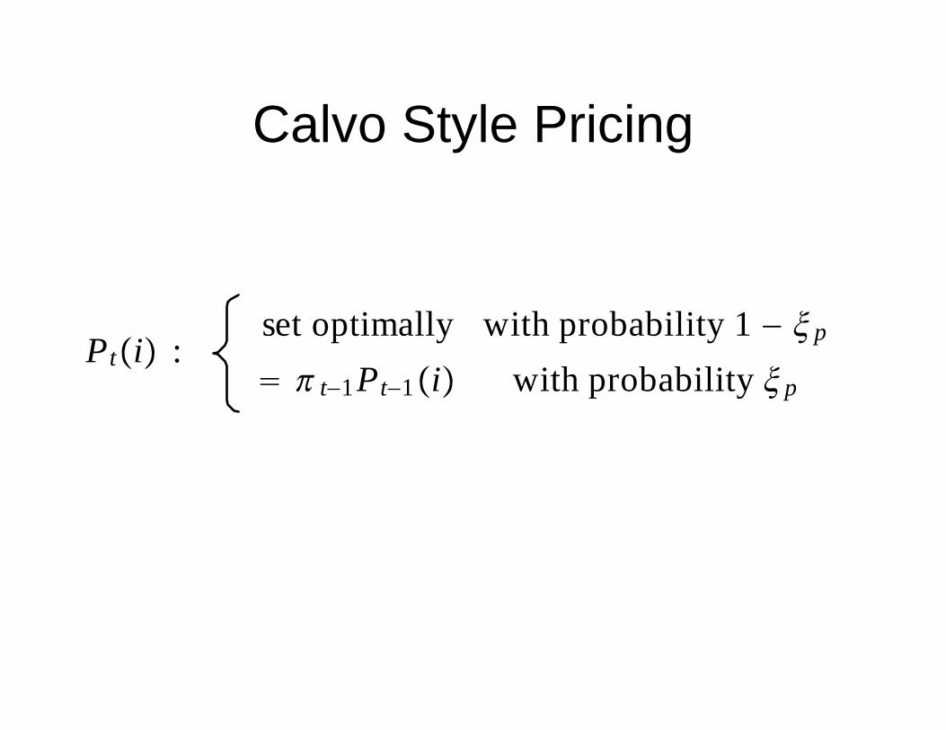
Calvo Style Pricing

Pti :set optimally with probability 1 − p

t−1Pt−1i with probability p

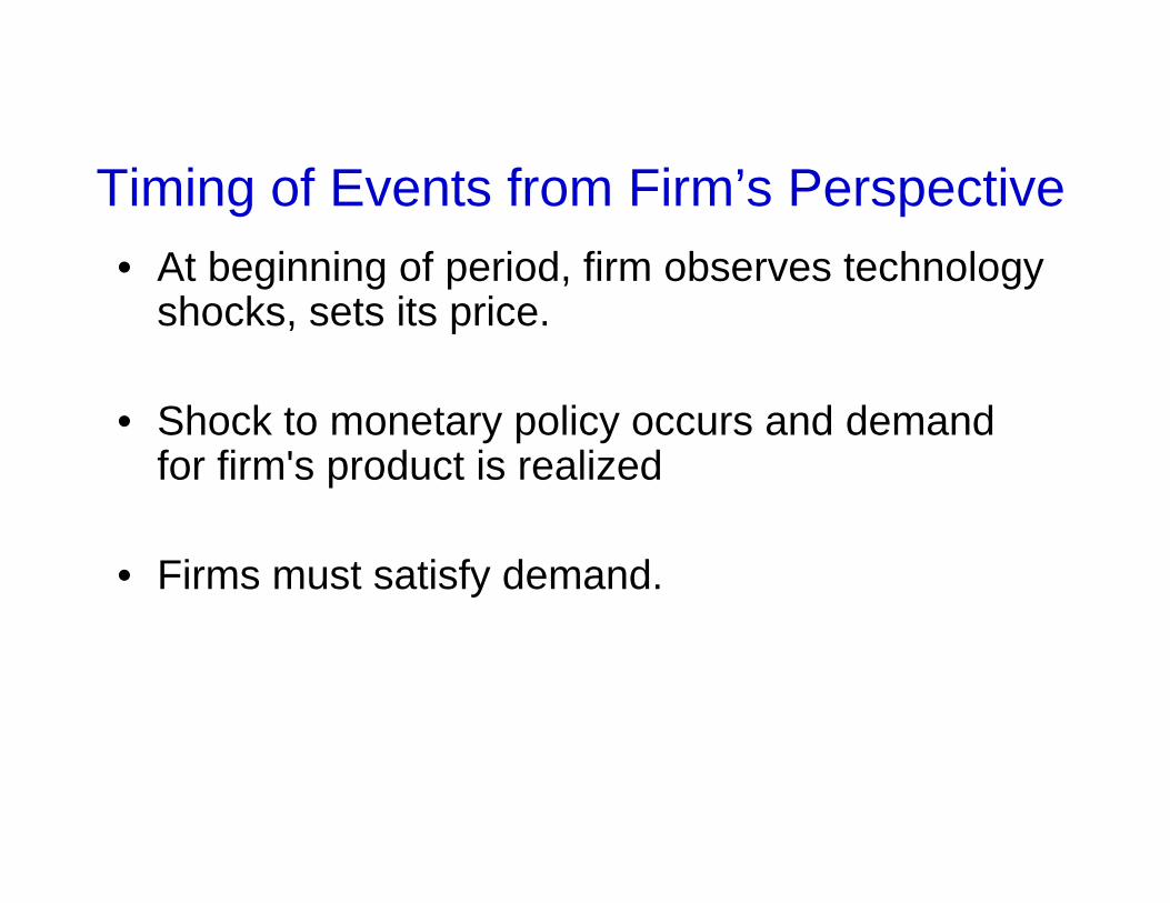
Timing of Events from Firm’s Perspective• At beginning of period, firm observes technology

shocks, sets its price.

• Shock to monetary policy occurs and demand for firm's product is realized

• Firms must satisfy demand.

Labor Market

• Perfectly competitive labor contractor hires differentiated labor services

• Sells homogeneous labor

subject to

maxWtHt − 01

hjtwjtdj

Ht 0

1hj,t

1w dj

w

, 1 ≤ w .

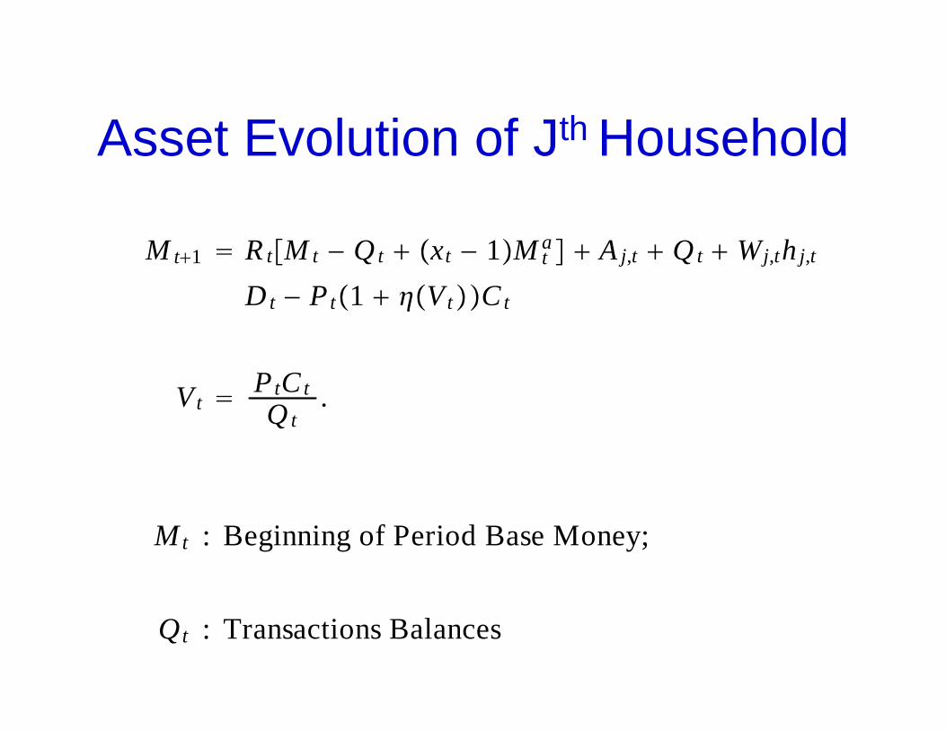
Asset Evolution of Jth Household

M t1 R tM t − Qt xt − 1M ta A j,t Qt Wj,th j,t

D t − Pt1 VtCt

Vt PtCtQ t

.

Mt : Beginning of Period Base Money;

Qt : Transactions Balances

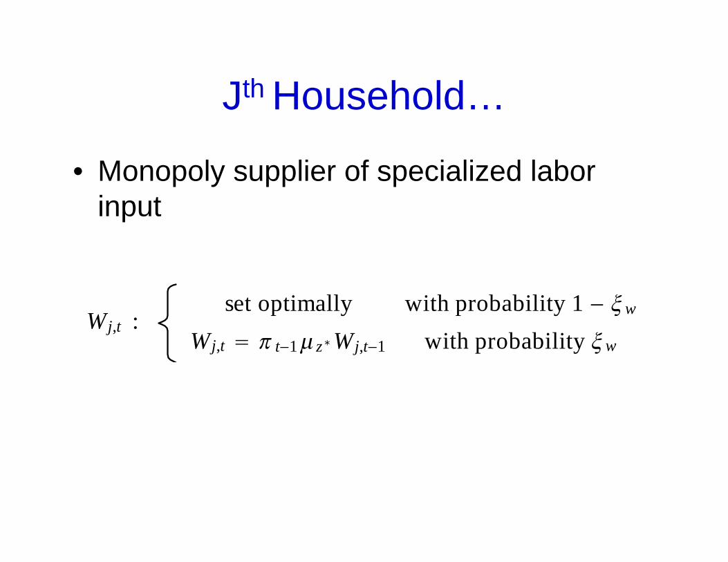
Jth Household…

• Monopoly supplier of specialized labor input

Wj,t :set optimally with probability 1 − w

Wj,t t−1 z∗Wj,t−1 with probability w

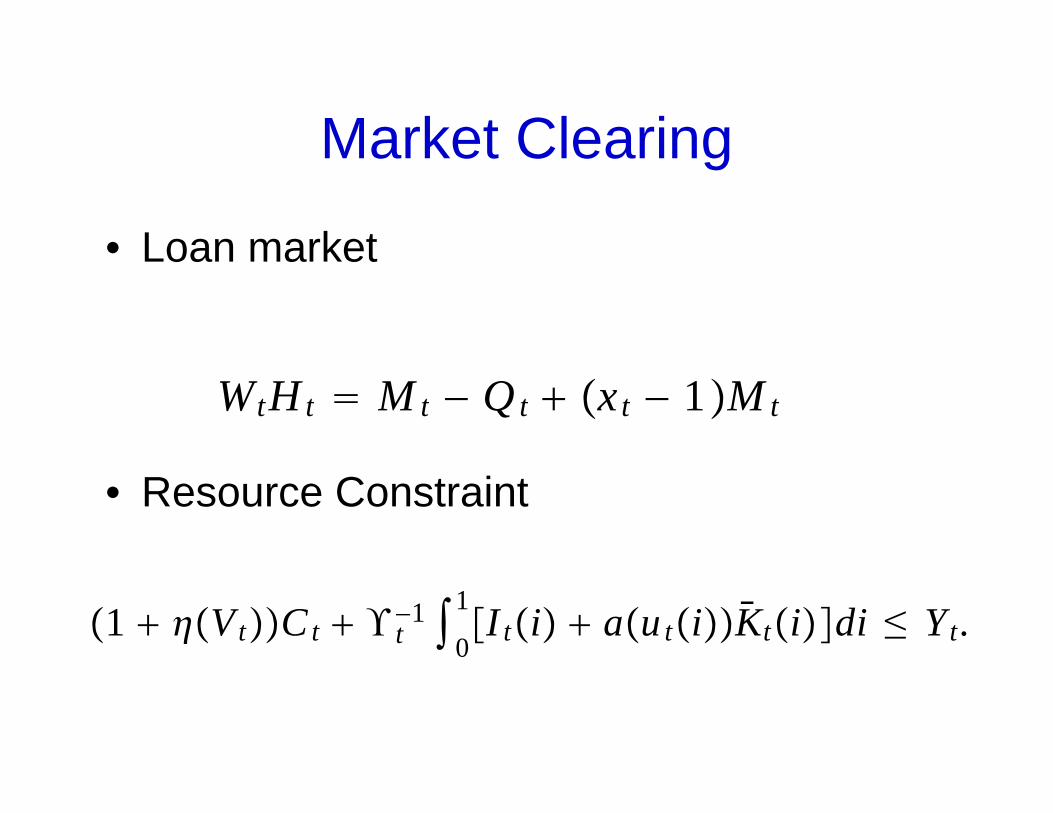
Market Clearing

• Loan market

• Resource Constraint

WtHt M t − Qt xt − 1M t

1 VtCt t−1

0

1I ti autiKtidi ≤ Yt.

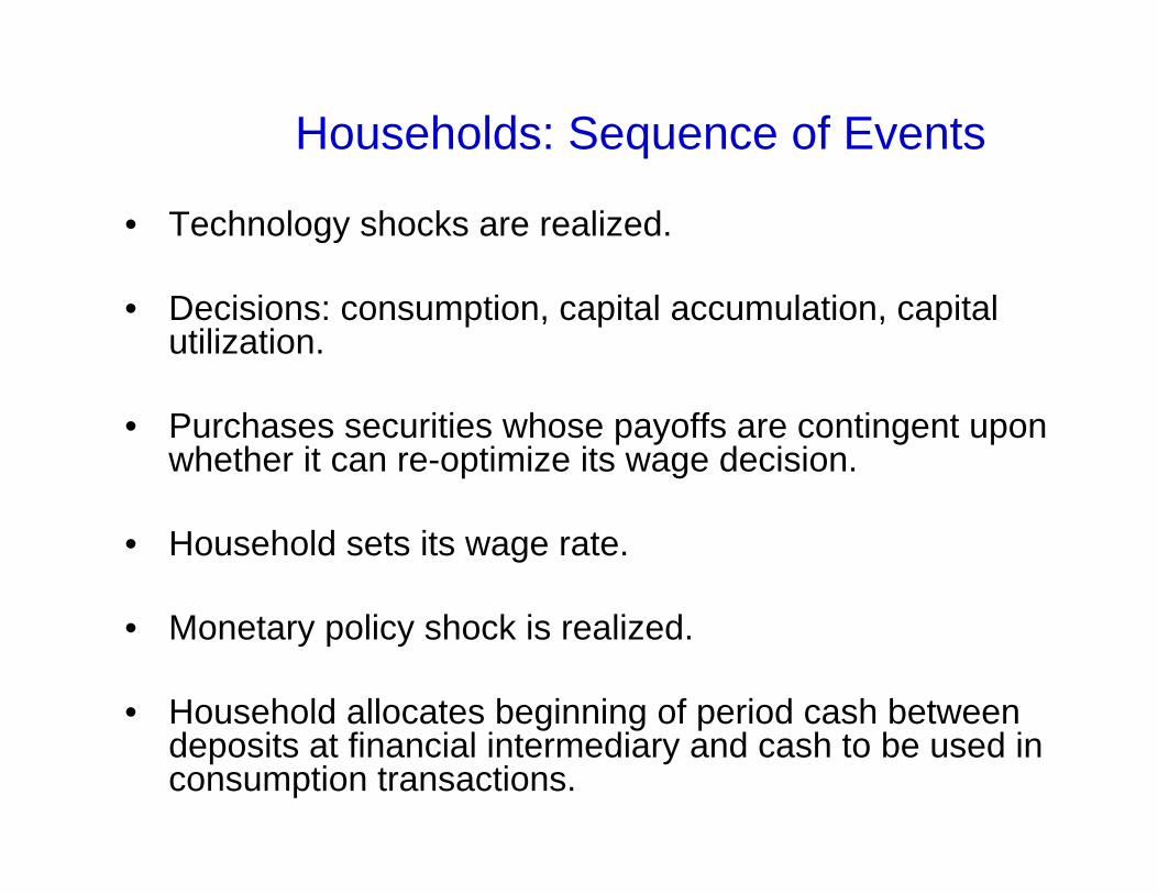
Households: Sequence of Events

• Technology shocks are realized.

• Decisions: consumption, capital accumulation, capital utilization.

• Purchases securities whose payoffs are contingent upon whether it can re-optimize its wage decision.

• Household sets its wage rate.

• Monetary policy shock is realized.

• Household allocates beginning of period cash between deposits at financial intermediary and cash to be used in consumption transactions.

Exogenous Shocks• Disembodied Technology

• Investment Specific

z tz t−1

zt

z,t z z,t−1 z ,t, z,t ≡ z,t− z z

t t−1

t

,t ,t−1 ,t .

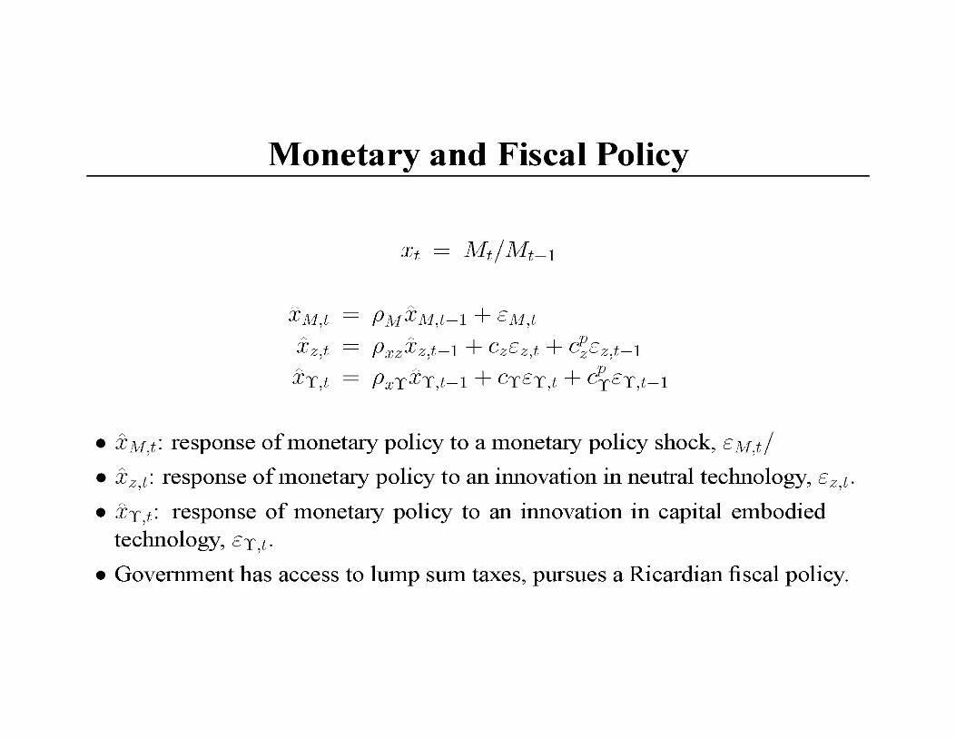
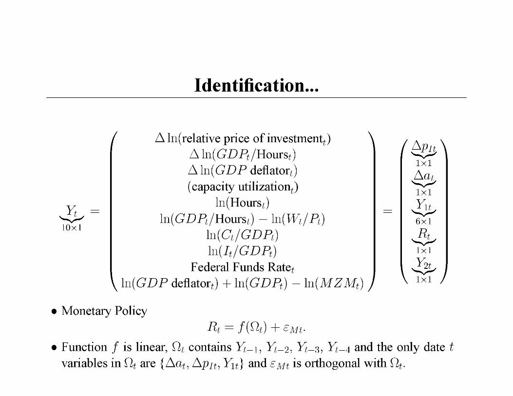
Key Identifying Assumptions• Monetary Policy Shock

Rt = f(Ωt) + εt

• Neutral and Capital Embodied Technology Shocks – The only shocks that affect the long run level of labor productivity

• Capital Embodied Technology Shocks– The only shocks that affect the long run price of investment

goods relative to consumption goods.

• These assumptions are satisfied in our model.

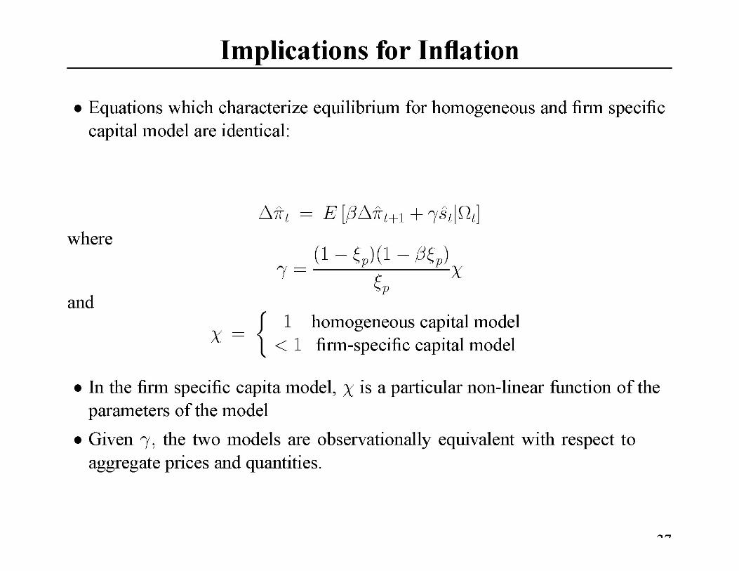
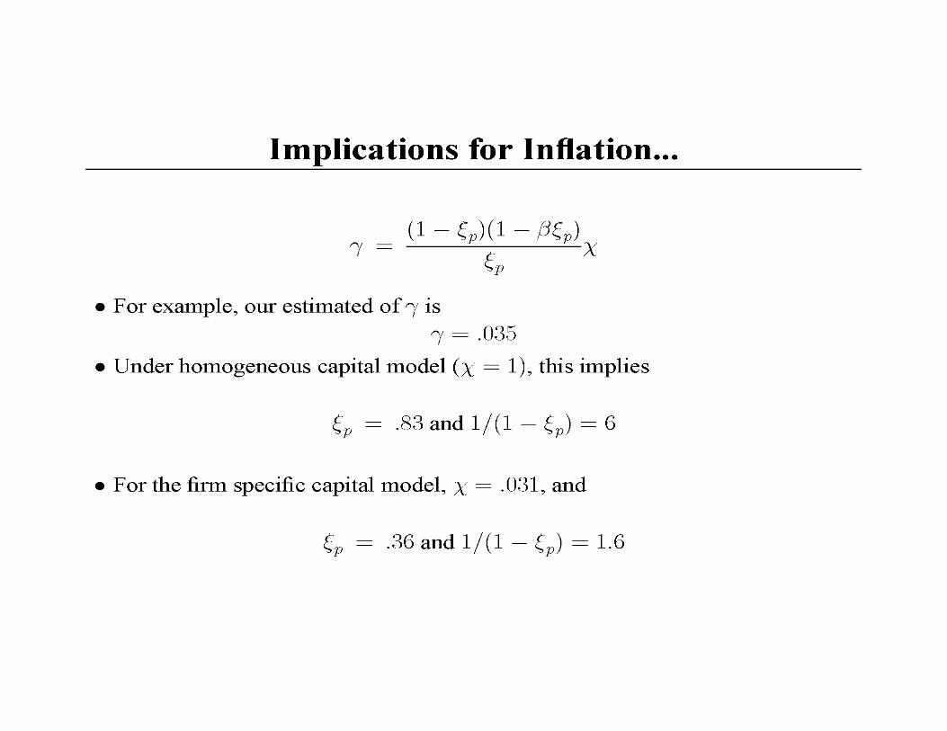
Implications for Wage and Price Re-Optimization

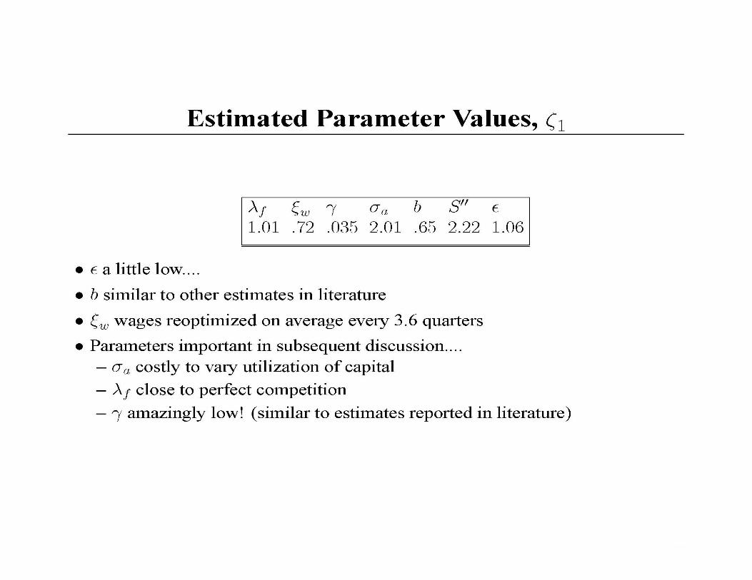
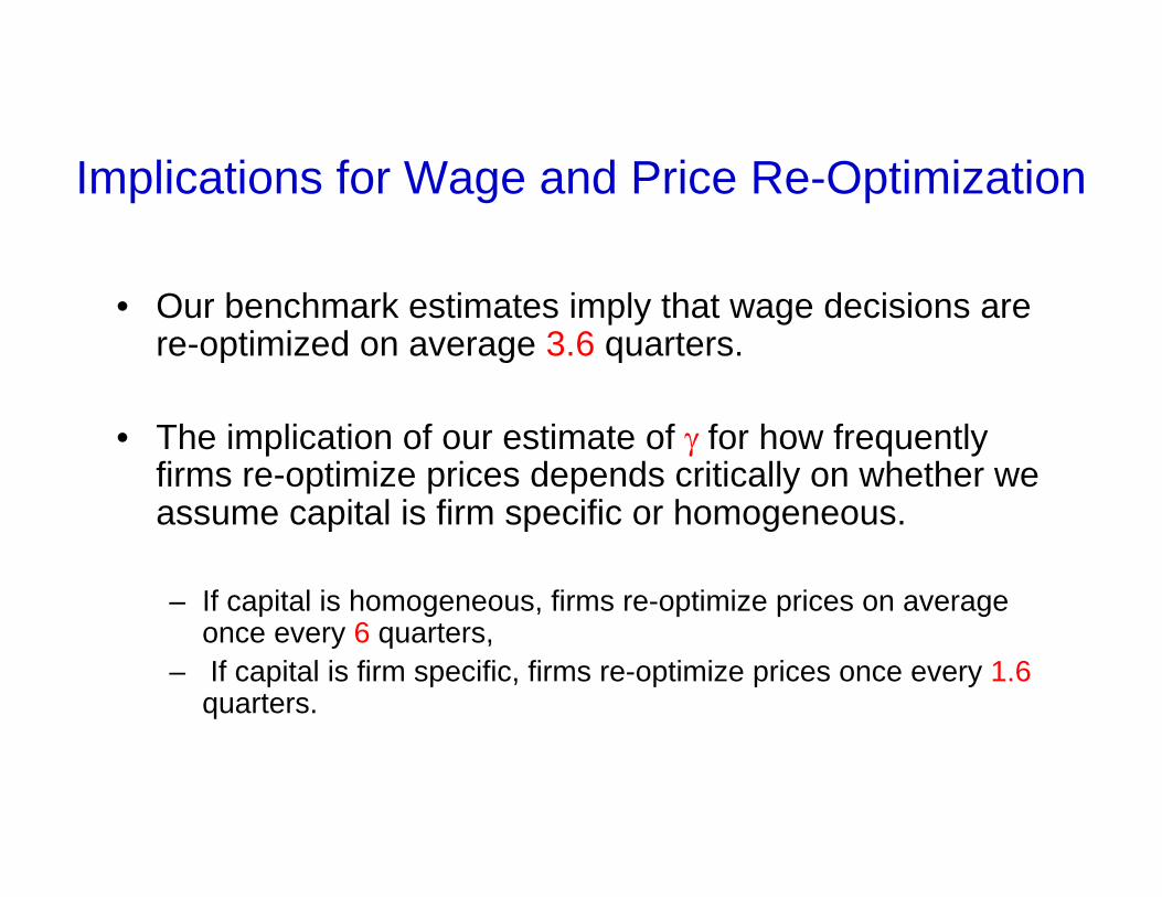
• Our benchmark estimates imply that wage decisions are re-optimized on average 3.6 quarters.

• The implication of our estimate of γ for how frequently firms re-optimize prices depends critically on whether we assume capital is firm specific or homogeneous.

– If capital is homogeneous, firms re-optimize prices on average once every 6 quarters,

– If capital is firm specific, firms re-optimize prices once every 1.6quarters.

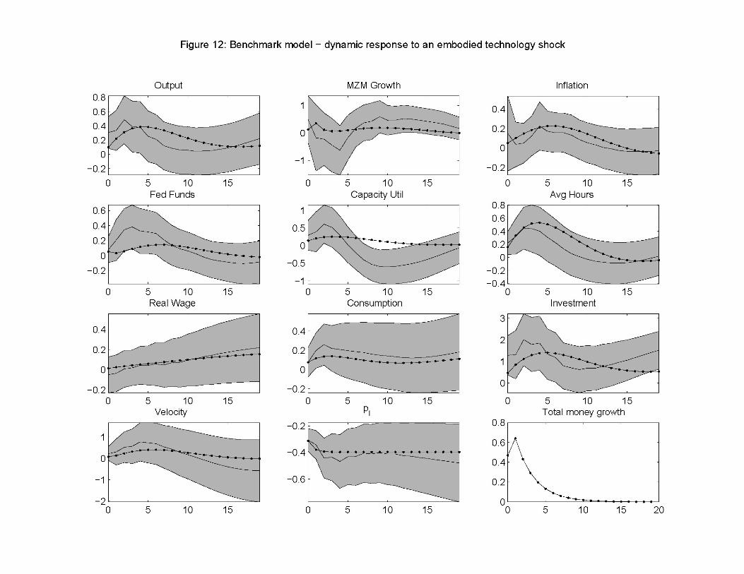
Monetary Policy and Technology Shocks

• How would the economy respond to technology shocks if monetary policy wasn’t accommodative?

• Monetary policy accommodates positive neutral and capital technology shocks.

• According to our model, in absence of monetary accommodation,

– Output and hours would fall in the wake of a positive neutral technology shock;

– Output and hours worked would rise by much less than they actually do after a positive capital embodied technology shock.

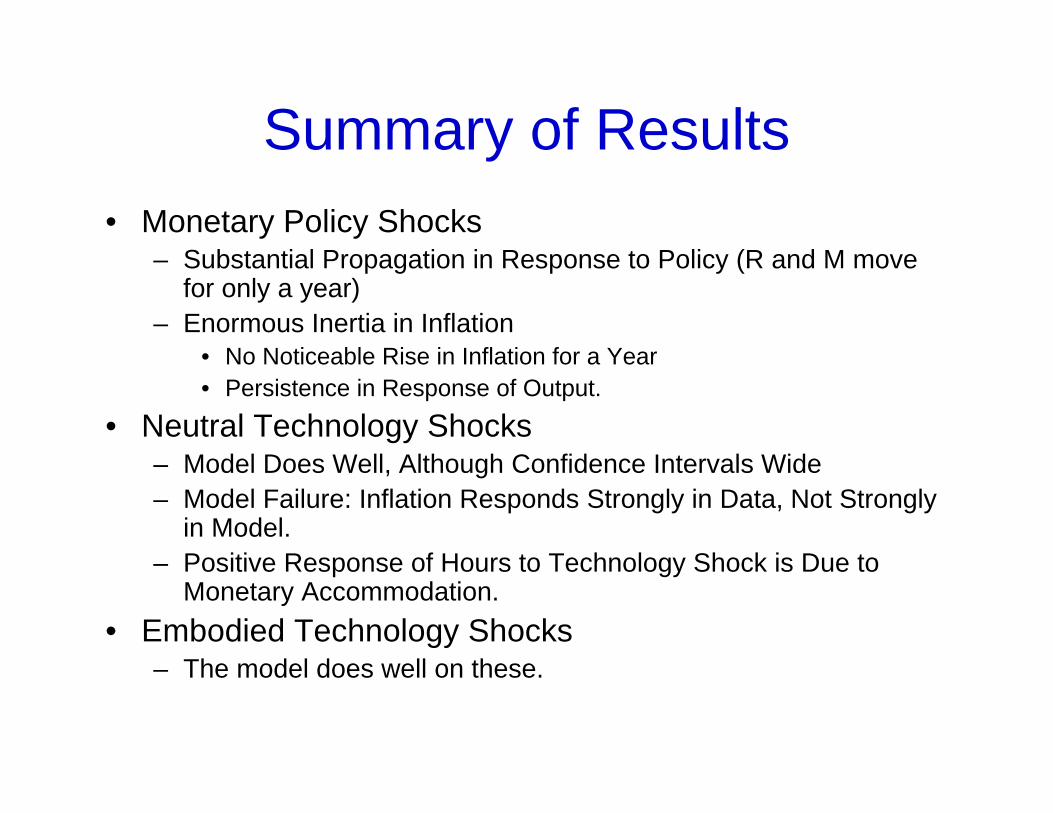
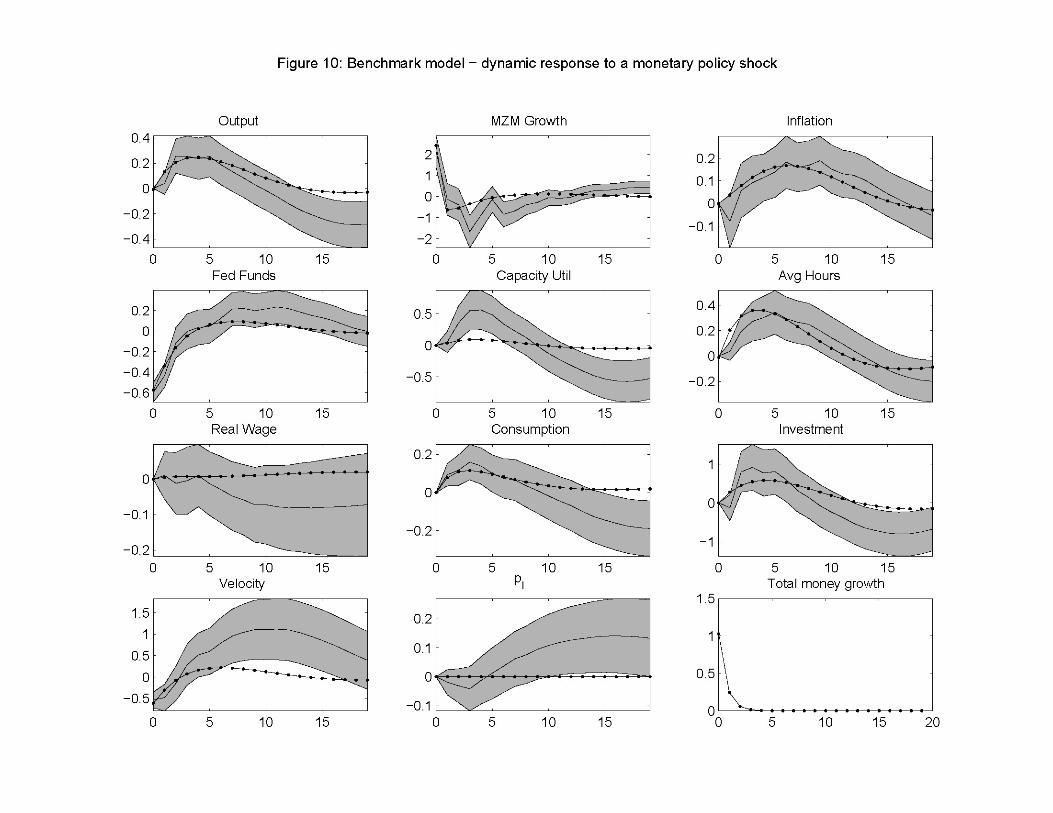
Summary of Results• Monetary Policy Shocks

– Substantial Propagation in Response to Policy (R and M move for only a year)

– Enormous Inertia in Inflation• No Noticeable Rise in Inflation for a Year• Persistence in Response of Output.

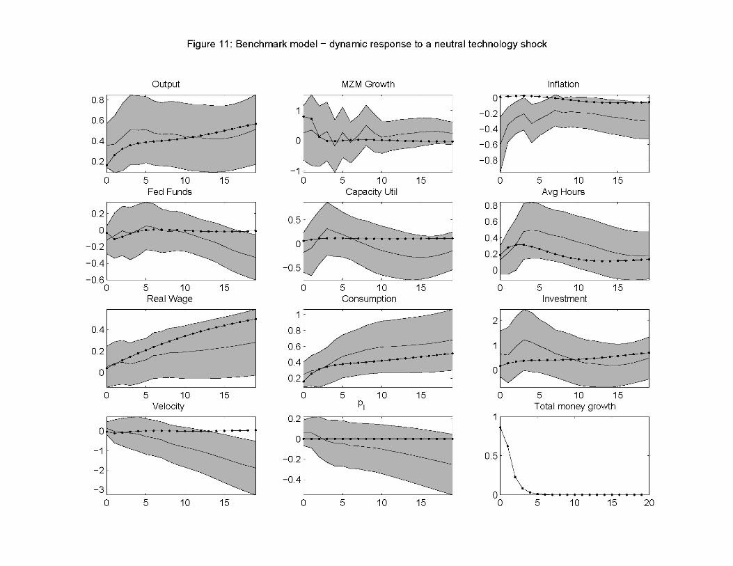
• Neutral Technology Shocks– Model Does Well, Although Confidence Intervals Wide– Model Failure: Inflation Responds Strongly in Data, Not Strongly

in Model.– Positive Response of Hours to Technology Shock is Due to

Monetary Accommodation. • Embodied Technology Shocks

– The model does well on these.

Lessons From the Analysis

• Frictions in Price Setting Not Important for Aggregate Dynamics

– Just a Small Amount Will Do

• This Finding Based on Analysis of Estimated GE Model

• For Our Results To Be Credible, Model Must Be Consistent With Basic Business Cycle Facts

Lessons From the Analysis….

• Basic Labor Market Facts:– Real Wages Not Very Cyclical, But Hours Worked Are

• Labor Wedge Is Cyclical– Any Successful Business Cycle Model Must Be Consistent

With These Facts• Parkin, Hall, Mulligan, Gali-Gertler-Lopez-Salido, CKM.

• We Accounted For Labor Market Wedge in a Parsimonious Way

• Conjecture:– Our Results About the Limited Importance of Sticky Prices

Will Be Robust to Alternative Ways of Capturing the Labor Wedge

Question

• We fit Impulse Responses Reasonably Well, But Do We Have Any Reason toTrust Them?

• Obvious Experiment:– What if the Estimated Model were literally true, How Well Would Our

Procedure Work?– We Plan to Study the Sampling Distribution of our Parameter Estimator– For Now, We Repeated the RBC analysis Described Above.

47

Plan

• Basic Idea: Generate Data from DSGE Model and Fit VARs in Artificial Data• Problem:

– DSGE Model Has Too Few Shocks– Empirical Procedure Recognizes We’re Short on Shocks and Offers a

Natural Solution

48

Background

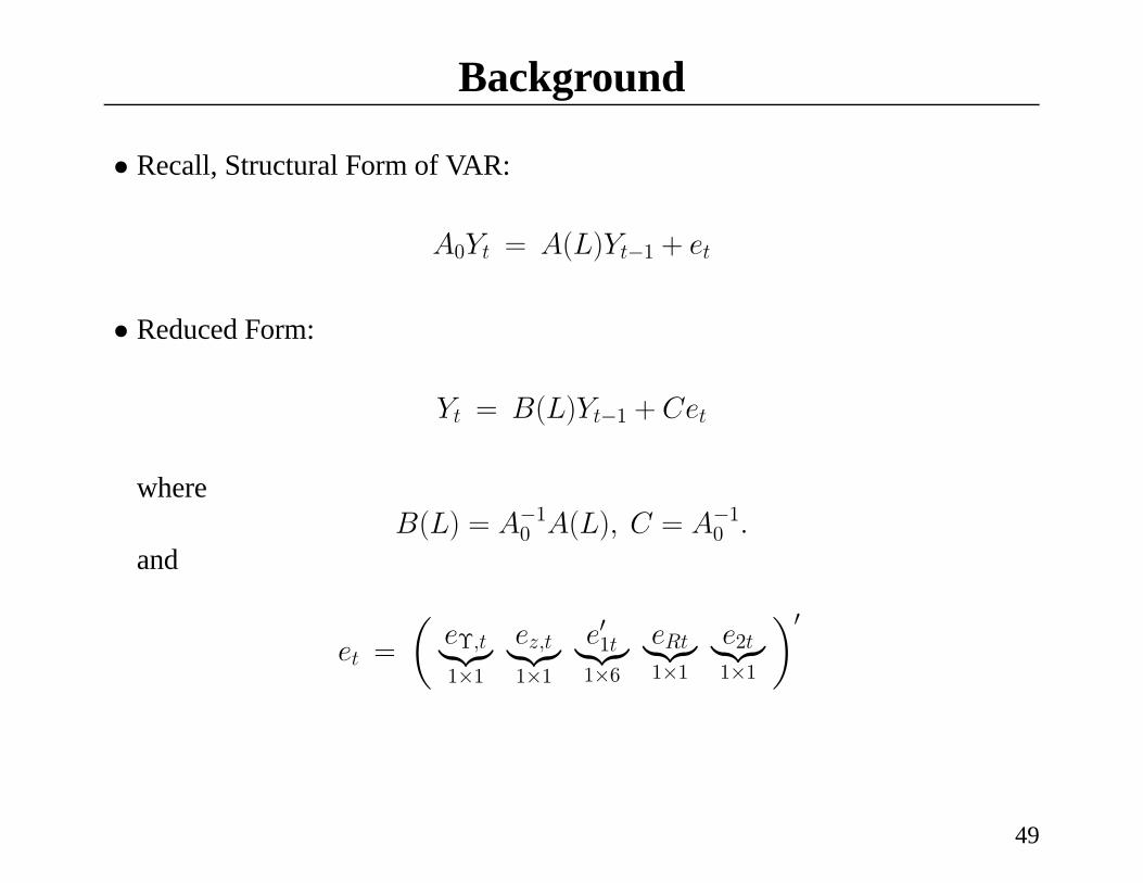
• Recall, Structural Form of VAR:

A0Yt = A(L)Yt−1 + et

• Reduced Form:

Yt = B(L)Yt−1 + Cet

whereB(L) = A−10 A(L), C = A−10 .

and

et =

µeΥ,t|z1×1

ez,t|z1×1

e01t|z1×6

eRt|z1×1

e2t|z1×1

¶0

49

50

Background ...

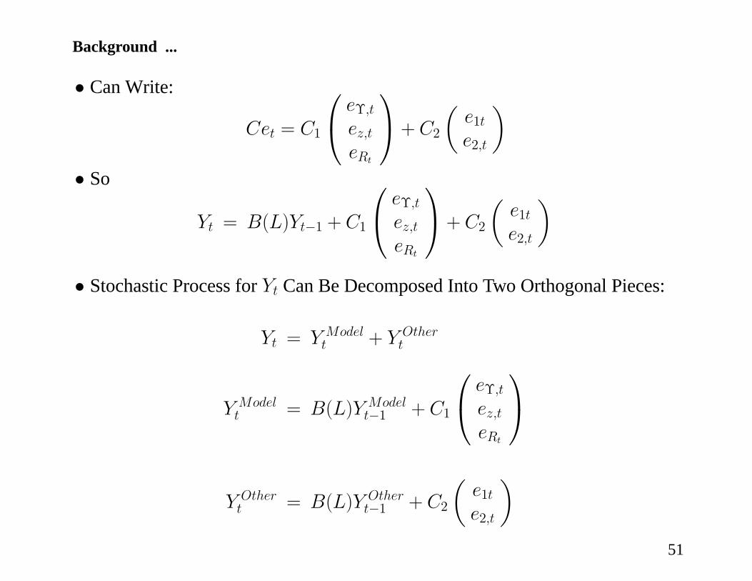
• Can Write:

Cet = C1

⎛⎝ eΥ,tez,teRt

⎞⎠+ C2

µe1te2,t

¶• So

Yt = B(L)Yt−1 + C1

⎛⎝ eΥ,tez,teRt

⎞⎠+ C2

µe1te2,t

¶• Stochastic Process for Yt Can Be Decomposed Into Two Orthogonal Pieces:

Yt = Y Modelt + Y Other

t

Y Modelt = B(L)Y Model

t−1 + C1

⎛⎝ eΥ,tez,teRt

⎞⎠

Y Othert = B(L)Y Other

t−1 + C2

µe1te2,t

¶51

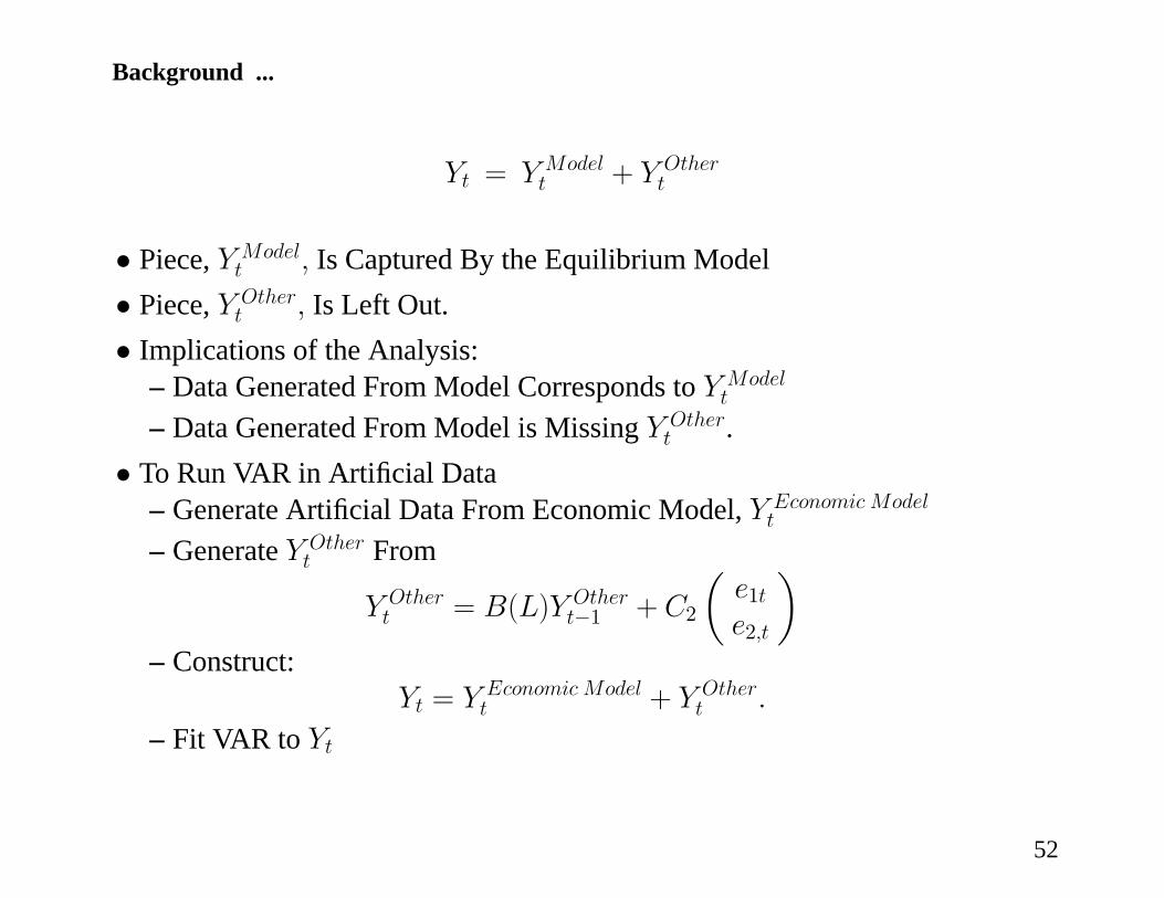
Background ...

Yt = Y Modelt + Y Other

t

• Piece, Y Modelt , Is Captured By the Equilibrium Model

• Piece, Y Othert , Is Left Out.

• Implications of the Analysis:– Data Generated From Model Corresponds to Y Model

t

– Data Generated From Model is Missing Y Othert .

• To Run VAR in Artificial Data– Generate Artificial Data From Economic Model, Y Economic Model

t

– Generate Y Othert From

Y Othert = B(L)Y Other

t−1 + C2

µe1te2,t

¶– Construct:

Yt = Y Economic Modelt + Y Other

t .

– Fit VAR to Yt

52

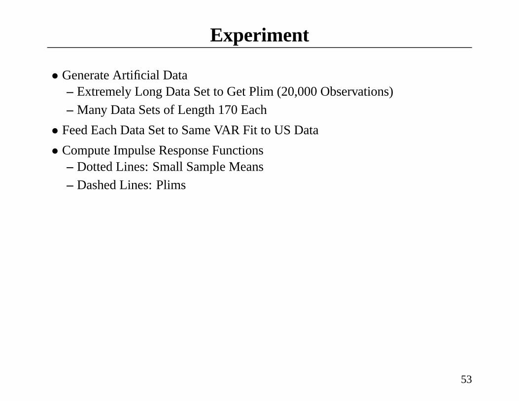
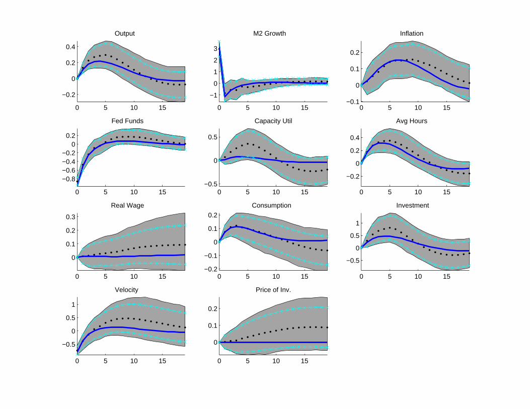
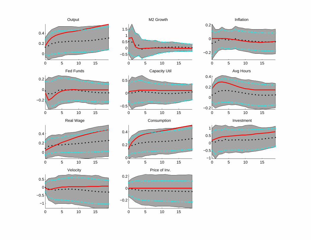
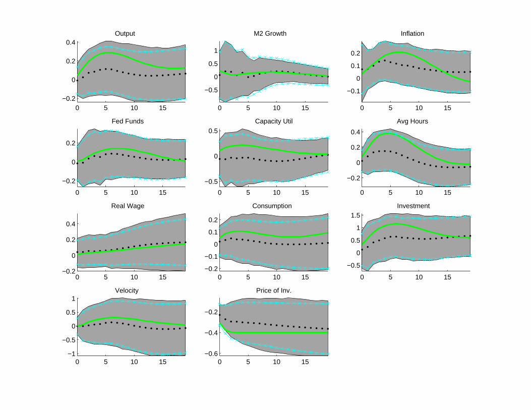
Experiment

• Generate Artificial Data– Extremely Long Data Set to Get Plim (20,000 Observations)– Many Data Sets of Length 170 Each

• Feed Each Data Set to Same VAR Fit to US Data• Compute Impulse Response Functions

– Dotted Lines: Small Sample Means– Dashed Lines: Plims

53

0 5 10 15

−0.2

0

0.2

0.4

Output

0 5 10 15

−1

0

1

2

3

M2 Growth

0 5 10 15−0.1

0

0.1

0.2

Inflation

0 5 10 15

−0.8−0.6−0.4−0.2

00.2

Fed Funds

0 5 10 15−0.5

0

0.5

Capacity Util

0 5 10 15

−0.2

0

0.2

0.4

Avg Hours

0 5 10 15

0

0.1

0.2

0.3

Real Wage

0 5 10 15−0.2

−0.1

0

0.1

0.2

Consumption

0 5 10 15

−0.5

0

0.5

1

Investment

0 5 10 15

−0.5

0

0.5

1

Velocity

0 5 10 15

0

0.1

0.2

Price of Inv.

0 5 10 15

0

0.2

0.4

Output

0 5 10 15

−0.5

0

0.5

1

1.5

M2 Growth

0 5 10 15

−0.2

0

0.2Inflation

0 5 10 15

−0.2

0

0.2

Fed Funds

0 5 10 15

−0.5

0

0.5

Capacity Util

0 5 10 15−0.2

0

0.2

0.4

Avg Hours

0 5 10 15

0

0.2

0.4

Real Wage

0 5 10 150

0.2

0.4

Consumption

0 5 10 15−1

−0.5

0

0.5

1

Investment

0 5 10 15

−1

−0.5

0

0.5

Velocity

0 5 10 15

−0.2

0

0.2

Price of Inv.

0 5 10 15−0.2

0

0.2

0.4Output

0 5 10 15

−0.5

0

0.5

1

M2 Growth

0 5 10 15

−0.1

0

0.1

0.2

Inflation

0 5 10 15

−0.2

0

0.2

Fed Funds

0 5 10 15

−0.5

0

0.5

Capacity Util

0 5 10 15

−0.2

0

0.2

0.4

Avg Hours

0 5 10 15−0.2

0

0.2

0.4

Real Wage

0 5 10 15−0.2

−0.1

0

0.1

0.2

Consumption

0 5 10 15

−0.5

0

0.5

1

1.5Investment

0 5 10 15−1

−0.5

0

0.5

1Velocity

0 5 10 15−0.6

−0.4

−0.2

Price of Inv.