Association for Information SystemsAIS Electronic Library (AISeL)

ICIS 1989 Proceedings International Conference on Information Systems(ICIS)

1989

MIS AND INFORMATION ECONOMICS:AUGMENTING RICH DESCRIPTIONSWITH ANALYTICAL RIGOR ININFORMATION SYSTEMS DESIGNAnitesh BaruaCarnegie Mellon University

Charles H. KriebelCarnegie Mellon University

Tridas MukhopadhyayCarnegie Mellon University

Follow this and additional works at: http://aisel.aisnet.org/icis1989

This material is brought to you by the International Conference on Information Systems (ICIS) at AIS Electronic Library (AISeL). It has been acceptedfor inclusion in ICIS 1989 Proceedings by an authorized administrator of AIS Electronic Library (AISeL). For more information, please contactelibrary@aisnet.org.

Recommended CitationBarua, Anitesh; Kriebel, Charles H.; and Mukhopadhyay, Tridas, "MIS AND INFORMATION ECONOMICS: AUGMENTINGRICH DESCRIPTIONS WITH ANALYTICAL RIGOR IN INFORMATION SYSTEMS DESIGN" (1989). ICIS 1989 Proceedings.29.http://aisel.aisnet.org/icis1989/29

MIS AND INFORMATION ECONOMICS: AUGMENTING RICHDESCRIPTIONS WITH ANALYTICAL RIGOR IN

INFORMATION SYSTEMS DESIGN

Anitesh BaruaCharles H. Kriebel

Tridas MukhopadhyayGraduate School of Industrial Administration

Carnegie Mellon University

ABSTRACT

Assessing the economic impacts of alternative Information System (IS) designs and selecting IS designparameter values for a given decision setting are two important research issues in the domain ofInformation Systems. Evaluation studies based on information economics provide rigorous butrestricted models, while traditional MIS studies suggest richer but less formal evaluation frameworks. 'In this paper, we attempt to combine the analytical rigor and descriptive richness into a unified andconsistent basis for evaluating IS designs and making design modifications (improvements) to existingIS. Expanding on the concepts of information economics, a multi-dimensional mathematical model ofinformation quality is developed. Several properties of the quality model with implications for systemdesign are derived in the form of propositions. The impacts of information quality differential upon theeffectiveness of an operational level decision setting are investigated through a decision-theoreticapproach. Next, a hierarchical model is suggested for relating system design variables to the quality ofinformation generated by the IS. Based on the quality differential impact analysis and the hierarchicalmodel, a structured methodology for making design changes to existing IS is outlined.

1. INTRODUCTION the quantitative models and the realistic features of theMIS approach. Expanding on the concept of"information

Two distinct but related issues in the domain of Informa- structures," we develop a mathematical model of informa-tion Systems (IS) are system design and evaluation. What tion quality. The economic impacts of the informationare the criteria on which alternative IS designs should be quality differential on the decisions utilizing the informa-evaluated? How should the design parameters of an IS be tion are determined. Some properties of the informationdetermined for a given context of use? These have quality model with implications for the system designer areremained two key research questions in the field for many derived. For example, we show how less detailedl informa-years. A review of the relevant literature reveals two tion (which is cheaper to obtain) can lead to the samecategories of research, based on information economics payoff for a class of decision problems. Counter-intuitive(Feltham 1968; Hilton 1981; Marschak 1963, 1971; Mar- results, such as reduced payoffs with increased reportingschak and Radner 1972; Merkhofer 1977) and traditional frequency, and the conditions under which such problemsMIS approaches such as the user satisfaction method are circumvented are obtained. We also provide an(Bailey and Pearson 1983; Epstein and King 1982; Nolan exposition of the design tradeoffs in the choice of informa-and Seward 1974; Zmud 1978). Information economics tion attribute values. Building on the impacts analysis, weprovides a rigorous methodology for evaluating "informa- propose a structured methodology for making designtion structures" in terms of a single criterion called improvements to existing systems. As a typical example'fineness" (Marschak and Radner 1972). The MIS litera- of an operational level decision setting, we use a produc-ture, although not mathematically as precise as information tion scheduling scenario as the reference context.economics, suggests numerous information attributes orcriteria that are not considered by the information econo- 2. MOTIVATION AND PRIOR RESEARCHmics models. Clearly, there exists a gap between the rigorof information economics models and the richness of the Many IS evaluation techniques employ user satisfaction asMIS studies. a surrogate measure of system effectiveness (Bailey and

Pearson 1983; Ives, Olson and Baroudi 1983; Nolan andIn this paper, we attempt to develop a unified and theoreti- Seward 1974; Powers and Dickson 1973). While thiscally sound basis for the evaluation and design of IS used approach measures the users' satisfaction with an IS,in operational level decision making. One of the goals of assessing the economic impacts of the lS is beyond thethis research is to preserve both the analytical precision of scope of this method (Chismar, Kriebel and Melone 1985).

327

In information economics, there has been rigorous research for this separation of the IS and decision characteristics ison the "value of information" using an information attribute shown in Figure 1.called "fineness" (Marschak and Radner 1972). The"fineness" criterion provides a formal mechanism forcomparing "information structures." An "information IS Desip Su,Y,Imstructure" is an abstraction of an IS and may be charac- V//bks -* Cl lli/#Ik' --0

terized by a single "likelihood function." However, asindicated by MIS studies (Adams 1975; Davis 1974; Emery  1971; Epstein and King 1982; Powers and Dickson 1973;

ECUK»M: Ex'i,sk

ImpCS -IC> A.#,I.

Zmud 1978), an IS requires a multidimensional description,a feature not considered by the information economicsmodels. I**

0.'Ir=:'ics

Thus, it is evident that in spite of the existence of a bodyof literature, there is no generalized analytical model of Figure 1. A Conceptual Model for IS Design Analysis:

information quality and value. As emphasized by Kriebel Separation of Signal, System, andDecision Characteristics(1979), a consistent mathematical model of information

quality is the first step in the evaluation of an IS. The cruxof the evaluation problem lies in being able to measure theimpact of information quality differential upon the payoff The signals generated by an IS have a set of attributes,to the decision maker (DM) utilizing the information. In

which can be defined to be independent of any decision

this paper, one of our goals is to reduce the large informa- context, and may therefore be called int,insic attributes.

tion attribute set found in the literature into a parsi- The design variables are linked to the intrinsic attributesmoniousbut sufficient set of analytically precise definitions. via an intermediate level of variables, the subsystem

characteristics. In Section 7, the IS is represented as aThis precision eliminates redundant attributes, helps derive collection of subsystems. Each subsystem has certainpropositions with system design implications, and provides characteristics such as sampling and information updatinga method for calculating the dollar impacts of information time, processing accuracy, etc. (henceforth referred to asquality on the DM's decisions. Moreover, the proposed subsystem characteristics), which are determined by theanalysis can be used to make design improvements to design variables for that subsystem. The intuitive justifica-existing systems. tion for this three-level hierarchy consisting of designIn Section 3, we present a conceptual model for the variables, subsystem characteristics, and signal attributes isseparation of system and decision characteristics. We as follows. Typically, there are a large number of design

define a sufficient but parsimonious set of signal attributes variables for an IS. Dealing with these design variablesin Section 4 and outline a decision-theoretic method for directly makes design modification a difficult task. Theevaluating the impacts of information quality upon the intermediate level (subsystem characteristics) enables theDM's payoffs in Section 5. We discuss "subsystem charac- designer to perform "dominance analysis" and therebyteristics," design parameters and their general functional identify a small number of "dominant" design variables.

relationships to signal attributes in Section 6. In Section Together with the characteristics of the decision context,the signal attributes determine the DM's payoff (or cost).7, we provide a structured framework for choosing andMarschak and Radner (1972) analyzed the impacts ofsetting values of design parameters through "dominance

analysis." "fineness" of information structures on a DM's payoff. Inthis paper, the analysis is extended to incorporate multipledimensions of information quality and their impacts on the

3. SEPARATION OF SIGNAL, SYSTEM AND DM's expected payoff.DECISION CHARACTERISTICS

£1*insic attributes are payoff-relevant (P-R) descriptions

Evaluation of IS design involves consideration of two of intrinsic attributes: They indicate whether differencescomponents: the lS itself and the DM's environment. The

in signal attributes are relevant for a given decision setting.

IS designer determines the setting of design variables such For example, two systems may differ in terms of their

as the number of information processors, storage capacity accuracy and still yield the same payoff under certainand number of error detection mechanisms. The choice conditions. Extrinsic attributes are thus measured by the

impact of signal attribute differentials upon a particularof these variables, in turn, determines the attributes of decision context. Intrinsic attributes are stated in techno-information (signals) generated by the IS. The impacts ofthese attributes on the DM's effectiveness depend on the logical terms such as time, frequency, and probability ofcharacteristics of the decision setting. In order that the

error, while extrinsic attributes are stated in units of payoff

same set of definitions may be applied to any context, the C e.g., dollars). The designer of the system deals withdefinitions of design variables and signal attributes must be intrinsic attributes, while the economic impacts (extrinsic

independent of the decision setting. A conceptual model attributes) are of interest to the DM.

328

4. INTRINSIC ATTRIBUTES The attributes, 'reporting delay," "age of information," and"currency of information," can be derived from monitoring

In this section, we build on the MIS evaluation literature time. "Reporting delay" and "age of information" for anyand define a mathematically consistent set of intrinsic uncertainty source can be found by subtracting the corres-signal attributes. While we do not claim this set to ponding monitoring time element from signal timing andconstitute an exhaustive list, we show that it captures the current time respectively. "Currency of information" isessence of a large number of attributes found in the decision context dependent and can be defined as the timeliterature. We propose the following attribute set. at which the decision is taken minus the monitoring time.

1. Signal timing2. Reporting frequency 43 Signal Resolution3. Monitoring time (period)4. Signal resolution Definition 3: Let Sl and S2 be the sets of distinct states for5. Intrinsic accuracy IS 1 and 2 respectively. IS 1 is said to have a higher signal6. Intrinsic informativeness resolution compared to IS 2, if the following condition is

satisfied:These attributes are generally not independent of eachother. This non-orthogonality gives rise to interesting For all si €St 3si€S2 such that st C 62 (11)tradeoffs between the attributes, an issue discussed inSection 7 on design choices. Intuitively, the condition implies that system 1 reports

greater details either or both in terms of the number ofBefore defining the attributes, it is important to provide a uncertainty sources and the value ranges. For example, theblack-box description of an IS. An IS reports on several IS2 database may contain information on demand and leadsources of uncertainty (e.g., demand, inventory, lead times, time, a subset of the information content of the ISlraw material prices). A state of the world may be defined database (demand, lead time and prices), and thereforeas a vector of random variables associated with uncertainty have lower resolution. As a second example, system 1 maysources and is described by a set of signals, {y}, from the recognize every integer value of demand, while system 2IS. For every IS there is a set of states, {s} = S, that are may be sensitive only to low, medium and high ranges ofrecognized by the IS as being distinct. For example, one demand. Resolution also covers aggregation of informa-IS may report the exact lead time, while another may only tion (such as monthly versus weekly data, or total demandrecognize short and long lead time ranges. Generally, the versus demand for individual items).signals are not perfect, being contaminated with "noise."This noise is expressed in the form of a likelihood function3 Resolution does not consider the "noise" present in theA(yls),the probability of receiving ycY, given that s€S has information. For example, the system that reports demandoccurred (see Marschak and Radner 1972). for individual items is considered to have higher resolution

than the one reporting total demand, even though thelatter may have less "noise" due to a natural averaging

4.1 Signal Timing and Reporting Frequency effect. For systems that are noiseless with respect to theirstate partitions, resolution and "fineness" (as used by

Definition 1: Timing of a signal is the time at which the Marschak and Radner) have the same meaning:signal is received by a DM. The reporting frequency, f, isthe inverse of the time interval between the receipt of twosuccessive signals by a DM. 4.4 Intrinsic Accuracy

While it may seem natural to associate reporting frequency Definition 4: For two systems differing only in terms ofwith repetitive decision making, in Section 6, we show how their likelihood functions, one is called intrinsically morereporting frequency can be important for a single.decision accurate than the other only if it is Blackwell sufficient forsetting. the other (Blackwell 1953; Hilton 1981). Let system i have

a likelihood function A(yi Is), i = 1,2. {s} = S is the set ofdistinct states for the two IS, and {Yi} = Yi is the signal setof system i. Since S and Y can be continuous or discrete

4.2 Monitoring Time (Period) sets, we use the integral sign to denote a generalizedsummation operator. Of course, any coarsening of S or Y

Definition 2: Let an IS monitor the states of uncertainty is discrete. System 1 is intrinsically more accurate orsources 1, N at times tltN respectively. The set of these Blackwell sufficient for system 2 if a stochastic transforma-times is called the monitoring time of the IS. If the tion g(yi,yi) exists for which the following are satisfied:monitoring of an uncertainty source, i, takes place from tito ti'' then the interval [ti, ti'l is used to denote the moni-

A(Yuls) = f g(yl,yDA(yl Is) Vs£ S VY2fY2 (2)toring period for i. yl€Yi

329

g<Yl,Yj = 1 Vyi€Yi (3) with respect to {s}.If A(wiil 81) 00 for j 01, then intm·parlition noise exists

Y2£Y2

g(yi,yj < 00 VY2€Y2 (4) more informative than a noiseless system (with lowerProposition 1: A noisy system with higher resolution is

Yl EY: resolution) if the noise is only intra-partition type.

More intuitively, one system is more accurate than the Proof: Let {y} be the signal set corresponding to {s} inother if the latter can be realized from the former through the above definition. Using Definition 5, it is seen that aa stochastic transformation. The resolutions of the two stochastic transformation from {8} to {s}, given bysystems must be the same for a comparison of intrinsic g(v/k'yi) = 1 for i=k, and 0 otherwise, satisfies conditionsaccuracy. For example, it is meaningless to compare the 2,3 and 4.accuracies of the blind men, each of whom is describing adifferent part of the elephant. Discussion: This proposition shows that resolution can be

the sole determinant of informativeness when the noise canbe separated into disjoint components corresponding to the

4.5 Intrinsic Informativeness partition elements 4, i = 1,2,..,n. It provides a simple toolfor comparing the informativeness of a subset of IS without

The definition of intrinsic informativeness is the same as doing the complex sufficiency calculations.that of intrinsic accuracy with the restriction on resolutionremoved. Note that uncertainty about the true states ofthe world is introduced by differences in accuracy and 4.7 Mapping between the Proposed and Existingresolution. Thus informativeness is the net effect of these Attribute Setsdifferences. The importance of informativeness is that itallows us to compare a set of IS (with comparable resolu- Having defined the signal attributes, we provide a mappingtions) without reference to a decision context. Thus if ISl between these attributes and those mentioned in theis more informative than IS2, then this relationship holds literature. This comparison highlights the confusion thattrue for any setting. Therefore, conditions under which exists m a section of the evaluation literature due to mixingone system is more informative than another are of special of intrinsic and extrinsic attributes and decision characteris-interest to us. ' tics. It is not possible to show a mathematical correspon-

dence between the proposed attributes and those found inHigher resolution does not guarantee higher informative- the literature because many of the latter ones have notness. The noise present in the signals may affect informa- been defined precisely.tiveness significantly. Similarly, low noise alone cannotensure high informativeness, since resolution (level of From the table, we note that several attributes such asdetail) is the second determinant of informativeness. The timeliness, relevance, and redundancy, which have beenset of special cases where resolution is sufficient for classified as information attributes, are actually decisioninformativeness is discussed below. context dependent (extrinsic attributes). While intrinsic

attributes can be compared for two lS without referenceto a decision context, it is not meaningful to use extrinsic

4.6 Intra-Partition and Inter-Partition Noise attributes as dimensions of information quality.

Let {s} and {0} be partitions of a state space S and let -{ 8   have higher resolution than {s}. Let si =C e i,e'j, -.,em,} for all i as shown in Figure 2. Let {wii} be 5. EXTRINSIC AITRIBUTES: IMPACTS OFthe signal set corresponding to { Gii}· SIGNAL ATYRIBUTES

Two systems may differ in terms of their signal attributes;however, the difference in payoff to the DM due to this

1 44 1 4 1 L.1 1 attribute differential depends on the decision characteris-

le: 1 1.1ties. Thus, two systems with different signal timings may

8, yield the same payoff in certain situations. In that case,the two systems have the same "timeliness" (to be des-cribed as an extrinsic attribute), though the signal attri-

Figure 1 State Space Partitions with Comparable Resolution butes are different. This phenomenon is central to thenotion of payoff-relevance in that intrinsic attributedifferences may or may not cause a difference in the DM's

Definition 5: If 1(Wk| Blb = 0 for i 0 k and any 1 and j, payoff. When they do not, the attribute differences are notthen there is no mter-parna-on noise with respect to {s}. relevant to the context.

330

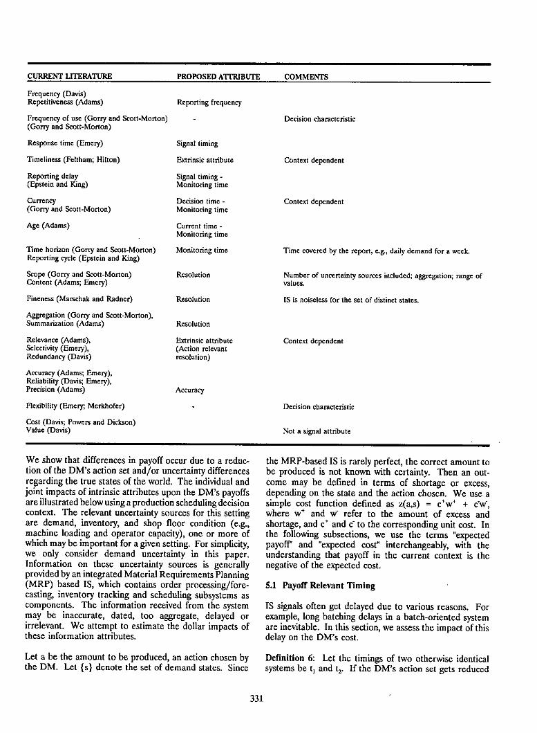
CURRENT LITERATURE PROPOSED ATTRIBUTE COMMENTS

Frequency (Davis)Repetitiveness (Adams) Reporting frequency

Frequency of use (Gorry and Scott-Morton) - Decision characteristic(Gorry and Scott-Morton)

Response time (Emery) Signal timing

Timeliness (Fellham; Hilton) Extrinsic attribute Context dependent

Reporting delay Signal timing -(Epstein and King) Monitoring time

Currency Decision time - Context dependent(Gorry and Scott-Morton) Monitoring time

Age (Adams) Current time -Monitoring time

Time horizon (Gorry and Scott-Morton) Monitoring time Time covered by the report, e.g., daily demand for a week.Reporting cycle (Epstein and King)

Scope (Gorry and Scott-Morton) Resolution Number of uncertainty sources included; aggregation; range ofContent (Adams; Emery) values.

Fineness (Marschak and Radner) Resolution IS is noiseless for the set of distinct states.

Aggregation (Gorry and Scott-Morton),Summarization (Adams) Resolution

Relevance (Adams), Extrinsic attribute Context dependentSelectivity (Emery), (Action relevantRedundancy (Davis) resolution)

Accuracy (Adams; Emery),Reliability (Davis; Emery),Precision (Adams) Accuracy

Flexibility (Emery; Merkhofer) Decision characteristic

Cost (Davis; Powers and Dickson)Value (Davis) Not a signal attribute

We show that differences in payoff occur due to a reduc- the MRP-based IS is rarely perfect, the correct amount totion of the DM's action set and/or uncertainty differences be produced is not known with certainty. Then an out-regarding the true states of the world. The individual and come may be defined in terms of shortage or excess,joint impacts of intrinsic attributes upon the DM's payoffs depending on the state and the action chosen. We use aare illustrated below using a production scheduling decision simple cost function defined as z(a,s) = c+w+ + c-w;context. The relevant uncertainty sources for this setting where w+ and w refer to the amount of excess andare demand, inventory, and shop floor condition (e.g., shortage, and c+ and c- to the corresponding unit cost. Inmachine loading and operator capacity), one or more of the following subsections, we use the terms "expectedwhich may be important for a given setting. For simplicity, payoff' and "expected cost" interchangeably, with thewe only consider demand uncertainty in this paper. understanding that payoff in the current context is theInformation on these uncertainty sources is generally negative of the expected cost.provided by an integrated Material Requirements Planning(MRP) based IS, which contains order processing/fore- 5.1 Payoff Relevant Timingcasting, inventory tracking and scheduling subsystems ascomponents. The information received from the system IS signals often get delayed due to various reasons. Formay be inaccurate, dated, too aggregate, delayed or example, long batching delays in a batch-oriented systemirrelevant. We attempt to estimate the dollar impacts of are inevitable. In this section, we assess the impact of thisthese information attributes. delay on the DM's cost.

Let a be the amount to be produced, an action chosen by Definition 6: Let the timings of two otherwise identicalthe DM. Let {s} denote the set of demand states. Since systems be tl and t2· If the DM's action set gets reduced

331

in the interval [ti,td, such that an action clement which isoptimal for some signal is lost, then the system with timing A(t) = i, 30-3t if t < 104 is considered more timely. The value of timeliness is the 0 if t > 10difference in the DM's expected payoff. Thus, if the actionset remains stationary in [tt,td, then the value of timelinessis zero. Let the DM's cost function be z = 10(a-s)2 and the

demand information system likelihood matrix be X(yi I si),An important subset of decision problems involves the ACY21 st), A(yi I sD, A(y,I sj = .6, .4, .4, .6 respectively.choice of numerical variables (e.g., the amount to produceor order in case of production or order schedules). In Before t = 4, A(t) does not become binding on the optimalmany situations, the maximum value of the variable that amounts to produce, and the total minimum cost is $240.can be chosen decreases with time. For example, with a Thus earlier signal timing has no impact before t = 4. Butgiven deadline, the maximum amount that can be produced for t=5 and 6, the expected cost increases to $245 andreduces with time. Similarly, for raw materials purchase, $340 respectively. In fact, it is not worth having the systema vendor may fill in orders on a FCFS basis. In that case.' (even if for free) with signal timing t > 6, since the DM'sorders placed later have a lower chance of getting filled in expected cost with a null system is $250.a given period. Let A(t) denote the maximum value of thedecision variable that can be chosen at t. Also, let p(s) bethe prior probability of s. 5.2 Payoff Relevant Accuracy

Proposition 2: With a stationary likelihood function.' Definition 7: For two systems differing only in terms ofearlier signal timing is preferred if their intrinsic accuracies, the value of payoff relevant (P-R)accuracy is the difference in expected payoffs (or costs)BA- < 0. given by expression (5) above, with Ak representing theat likelihood function of system k, k = 1,2 and with tl = t2-

Proof: The difference in expected costs due to signal From the definition of intrinsic accuracy, it can be notedtimings ti and ti can be shown to be that the payoff associated with a more accurate system is

at least as high as that from a less accurate system.(5)5.3 Payoff Relevant Reporting Frequency

E (-1)k+1   mink=1 yfY aE[OACED] · sfsz(a,s), (sly)p(y) Reporting frequency, f, depends on the type of system in

use. An on-line system displays information immediately,while a batch system reports only periodically. A deferred

where A(sly) = A(yls)p(s) / p(y) and the marginal on-line system has a reporting frequency in between thoseprobability of on-line and batch systems. For a single decision in a

given time frame [O,T] reporting frequency impacts become

A (y Is)p(s) and timing effects.subtle and can be thought of as a combination of accuracy

S€SSay a production decision has to be taken by T. If 1/f <

Since A(ti) > A(t2) for t2 > ti, if a > A(tb for any signal T, then the DM receives more than one signal (describingy, then expression (5) is less than zero, showing that the the state of the same uncertainty sources, though withexpected cost is lower for system 1. increasing accuracy) in [O,T], assuming that the first signal

is received at t = 0. When accuracy increases with timeDiscussion: This proposition provides a way to measure (due to a reduction in uncertainty over time), the nIh signalthe usefulness of a system on the basis of its signal timing. is always more accurate than the n-lth signal for n =The proposition implicitly indicates the possibility of a 1,2,..,n. However, if the maximum amount that can benoiseless system becoming inferior to a null system because produced, A(t), decreases over time, then the DM has toof the former's signal timing. A numerical example determine the optimal trade offbetween"good" actions andinvolving demand uncertainty follows. more accurate information. In particular, after receiving

a signal, the DM has to choose whether it is optimal toExample: Let there be two demand states st = 10 and take an action immediately (denoted b  a) or to wait fors2 = 20 with prior probabilities Pl = P2 = .5. Let the the next signal (denoted by B). If the P signal received atmaximum amount that can be produced be time variant time (i-1)/f is y, let it be denoted by Yi· The DM'sand be given by expected cost with a reporting frequency f is given by:

332

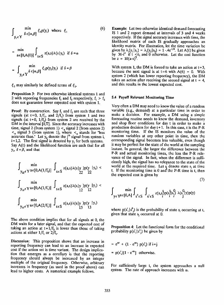
f min Cip(y) where f 1 (6) Example: Let two otherwise identical demand forecasting6 6 [ot,B] IS 1 and 2 report demand at intervals of 3 and 4 weeks

Yl€Y respectively. If the signal accuracy increases with time, thelikelihood matrix of each IS gradually approaches anidentity matrix. For illustration, let the time variation be

min given by At(yl I st) = At(Y21 SD = 1 -.4e-": Let A(t) be given= a€[OA(0)1  SES z(a,s),(slyi) if 6 =01 by 36-t2 if t < 6, and 0 otherwise. Let the cost function

be z = 10(a-sjz.

- f minCa|p(Y2 | Yl) if 6 =B With system 1, the DM is forced to take an action at t = 3,

6 E [c,Bl because the next signal is at t=6 with A(6) = 0. WithY2€Y system 2 (which has lower reporting frequency), the DM

takes an action after receiving the second signal at t = 4,42 may similarly be defined terms of (3• and this results in the lowest expected cost.

Proposition 3: For two otherwise identical systems 1 and2 with reporting frequencies f, and fz respectively, fi > G 5.4 Payoff Relevant Monitoring Timedoes not guarantee lower expected cost with system 1.

Very often a DM may need to know the value of a randomProof: By construction. Say fi and G are such that three variable (e.g., demand) at a particular time in order tosignals (at t= 0, 1/fi, and 2/fi) from system 1 and two make a decision. For example, a DM using a simplesignals (at t -0, 1/fj from system 2 are received by the forecasting routine needs to know the demand, inventoryDM in the interval [O,T]. Since the accuracy increases with and shop floor conditions fur day t in order to make atime, signal 2 (from system 11) <a signal 2 (from system 2) production decision for day t + 1. In this case, t is the P-R<, signal 3 (from system 1), where <, stands for "less monitoring time. If the IS monitors the value of theaccurate than." Let Yi· denote the ith signal from system i, random variables at any other point in time, then thei = 1,2. The first signaJ is denoted by yi for both systems. corresponding signal becomes less valuable, even thoughSay A(t) and the likelihood function are such that for all it may be perfect for the state of the world at the samplingYi, 6 =B, and that instant. In general, the larger the difference between the

P-R and actual monitoring times, the less the P-R rele-vance of the signal. In fact, when the difference is suffi-ciently high, the signal has no releyance to the state of them in

722£YaE[OA(1/fjl  sfs z(a,s)A(sly )p(y lyl) <world at the required time. Let s denote state s  at time

22 22 t. If the monitoring time is 0 and the P-R time is t, thenthe expected cost is given by

(7)f min

y12£ yac [OA(1/ft)] · sfs z(a,S)A(s 1 2)PC 2|Yl) <

fy,yac[O,Al Jsoes s,ES Z(a,s )p(s 199 A(sgy)p(y)

min r rf min

y13fya€[O,AG/fi)1  sfs z(a,s)A(s | )P( 3 lyl)where p(st I soj) is the probability of state si occurring at t,given that state sj occurred at 0.

The above condition implies that for all signals at 0, theDM waits for a later signal, and that the expected cost oftaking an action at t = 1/4 is lower than those of taking Proposition 4: Let the functional form for the conditional

actions at either 1/4 or 2/fi. probability p(s i I s°j) be given by

Discussion: This proposition shows that an increase inreporting frequency can lead to an increase in expected = e" + (1 - em) p(sti) if i=jcost if the action set is time variant. The design implica-tion that emerges as a corollary is that the reporting = p(si,)[1 - e*,] otherwise.frequency should always be increased by an integermultiple of the original frequency. Otherwise, arbitraryincreases in frequency (as used in the proof above) can For sufficiently large L the system approaches a null

system. The rate of approach increases with a.lead to higher costs. A numerical example follows.

333

Proof: Let p(s') be the DM's prior probability density on The expected cost is given by{s} at t. Then as t -+ CO, p(sti I S j) -+ p(s i)

Therefore, VaV € > 0 3t such that I p(s'i) - p(sti 1 soj) 1 <  v i and j. Thus, for sufficiently small c, Le., for suffi-

f rnYn f

ciently large t, expression (7) tends to yey a€[OA] Js ES z(a,sp)A(sply)p(y)

min

fy,ya,[0.Als'£Sfs'¢ S z(a,s.5p(4ACS'ly)p(y)Example: A numerical example involving aggregation of

I l l information may be useful. Consider the demand for twomin f t t items 1 and 2 denoted by random variables xi and Xe

J z(a,s )p(s ) respectively. Let xi, X2 £ { 100,200}. Let the cost functionac[O,A] s'€S be given by z(at,22791,© = 4(a -X ) + 6(82-XD: Thus, thereare four P-R states. LEt an (xi,© = (100,100), (100,200),

which is simply the expected cost for a null system. With (200, 100), (200,200). Let an order processing systemlarger values of a and for a given value of £, t becomes aggregate the information by reporting the total demand.smaller and the system approaches the null system faster. The set of distinct states of this IS is given by {0} = {200,

300,400}. Let the prior density on the states be uniform.Discussion: The functional form of the conditional Also, let the system be noiseless with respect to {8}. Withprobability is fairly general in that, as t increases, the the system, the expected cost is found to be $12,500 withinformation on the state at time 0 becomes progressively a'l = a'z = 150. This is the (opportunity) cost of lower-irrelevant in predicting the state at t. a is a measure of the than-adequate resolution, since the cost with a perfectrate at which the relevance of the signal is lost. For system and just-adequate resolution is $0 in this example.example, if the demand for a product is highly variable,then the corresponding a has a small value, indicating thatthe relevance of the information is lost quickly. This 532 Cost of Higher-Than-Adequate Resolutionproposition indicates that it is desirable that the actualmonitoring time be close to the P-R time. Unfortunately, If e has higher resolution than Sp then some additionalthis may not always be feasible when long information effort is required upon the receipt of a signal in order toprocessing times and time variant action sets are involved. find the corresponding state in the P-R set Sp. In this case,In those cases, the monitoring may have to be done earlier the difference in cost is equal to the difference in the costto avoid a loss of timeliness of the signal. This concept is of additional information processing.further discussed with an example in Section 7 on designmodifications.

5.53 Action Relevant Resolution

5.5 Resolution Adequacy For a wide variety of decision problems, the level of detailrequired is coarser than the corresponding P-R levels. For

Definition 8: Let Sp denote the payoff-relevant set,of the example, consider a production system with two batchstates for a DM. Let e be the set of states considered as sizes: 50 and 80 units. Say demand can take four values,distinct by an IS. The resolution of the IS is just adequate 30, 50, 80 and 100 units. The P-R partition of the demandif 8 = Sp, lower or higher than adequate accordingly as e space has four corresponding elements. However, notehas lower or higher resolution than Sp. that the restricted optimal batch sizes are 50 units for any

one of the states 30 and 50 and 80 units for the states 80and 100 (assuming that the unit shortage cost is equal to

5.5.1 Cost of Lower-Than-Adequate Resolution the unit excess cost). Therefore, for this restricted actionset, an IS that cannot distinguish between the states 30 and

Let {8} = e have lower resolution than the P-R set {sp}. 50, and between 80 and 100 results in the same expectedTo determine the impacts of this resolution on the DM's cost as the one providing the P-R partition. We refer topayoff, we calculate the conditional probability A (sply) the less detailed IS as having the action-relevant (A-R)from A(@Iy), as resolution. This exposition is both interesting and impor-

tant because it shows the possibility of getting the same,(sply) = 0Ijp(sple),(ely) where

payoff (or cost) with less detailed information for a classof decision problems.

p(spi 8) = p(# Isp)p(sp) / f pce Isp)p(sp) and Definition 9: Let {ss} = Ss be the state space partition ofSp €Sp

an IS. This IS is said to have action relevant resolution, if,for every s., only one action is optimal for every state that

Vsp£Sp 38 £8 such that p(G Isp) = 1.may be contained in s,.

334

Proposition 5: Consider two IS, one with the A-R resolu- Next we turn to the subsystem level of the IS and study thetion and the other with higher resolution. Let the systems design tradeoffs involved.be noiseless with respect to their own state partitions. Theexpected payoff (or cost) difference between the two IS iszero.

6. INSIDE THE IS BLACK BOXProof: Referring to Figure 2, consider {s} and {8 } aspartitions with A-R and higher resolution respectively. Let 6.1 Subsystem Characteristicsz(a,G) be the cost function. Since the IS are noiseless withrespect to their set of distinct states, the expected cost with Conceptually, an IS may be represented as a collection ofa system that provides partition {9}i s given by the following subsystems: monitoring storing, processing

(transformation), retrieving and transmitting subsystems(see Marschak 1971). These are the fundamental informa-

I min z(a,#)p(8) tion handling activities, one or more of which can beBfe a [0441 identified in every IS. For example, a simple database

management system consists of storing, processing andretrieving subsystems.

I ,zcal,81)p(81) + I *4,82)P(,D + ···-1€St  2€52 The monitoring subsystem samples states of the world.

For example, machine loading, operator capacity andmaintenance routines may be monitored by the schedulingwhere a, is the optimal action corresponding to si. With subsystem of the MRP-based lS. The processing subsys-the A-R resolution, the expected cost is tem processes the monitoring data to create new informa-tion (e.g., the generation of parts list from customer order

I min y information) and/or transforms the monitoring data intos,€S a€A 8, s,z(a,ei)p(Oil©p(si) aggregate reports. The parts requirement subsystem of the

integrated MRP system is an example of the processingsubsystem. It takes as input order and forecasting informa-Note that p(#ilsi)p(si) is equal to p(s, 1 #i)p(Bi) and thattion and generates (through processing) raw materialp(4  #i) = 1 for all Gicsi. Therefore, the two expectedrequirements. The exact sequence of subsystems is not thecosts above are equal.same for every IS.

Discussion: Once the A-R level of detail is reached, moredetails are of no consequence to the decision context.

Each subsystem may be considered as an individual systemTherefore, any additional information is undesirable and described by certain attributes which are referred tobecause of the extra cost of more detailed information and as subsystem characteristics. For example, like the entire

IS itself, the monitoring subsystem has accuracy, frequency,the processing load placed on the DM. resolution, etc., as its attributes. These attributes are inturn determined by the design variables of the monitor.Proposition 6: For systems that are noiseless with respectThe general relationships between subsystem characteris-to their own state partitions, A-R partition is "weakly tics and signal attributes are discussed in the balance ofcoarser" (i.c., never finer) than P-R partition. this section.

Proof: Suppose not. Assuming that A-R partition is finerthan the P-R partition, let { # } and {si} (in Proposition 5) The accuracy of each subsystem may be represented by abe the A-R and P-R partitions respectively. Without lossof generality, assume that the A-R element {si} consists of likelihood function relating the inputs and outputs of thetwo P-R elements, 81, and 81. Let a* and a** be the - subsystem. For a serial architecture, let {s,} = Si denoteoptimal actions for the states 01, and 82 respectively. From the input set of distinct states fur subsystem i,i = 1,2,...,n.

P-R considerations, we have z(a*,8 <j = z(a*,81) and Note that {s,} is also the output set of stage i-1 fori = 2,3,...,n. Let A(4+1 J sl) denote the probability of theoutput state being sii+E, given that si is the input. If asubsystem is noiseless and does not induce a change inFrom A-R considerations, z(a*,eli) < z(a**,eli) andresolution, then A(. 1.) denotes an identity transformation.z(a**,822) < z(a*,82). This leads to a contradiction.For example, an ideal transmission subsystem should have

Discussion: Since more detailed information is generally this property.more costly, Proposition 6 indicates that for a class ofdecision problems, the A-R resolution is less detailed than The signals of the IS are generated by the last subsystem,the P-R resolution and is therefore cheaper to obtain. n. Combining the transitional probabilities for each

subsystem, the conditional probability of the signal beingPropositions 5 and 6 provide direct guidelines for selectingy, given that the input of subsystem 1 is sl, is obtained asthe information content in IS design.

335

7. SETTING DESIGN VARIABLES: "DOMINANCEA(Y IsO = f ...   A(ylsn)A(s»]sn-))...ACS21si) ANALYSIS"

S2€S2 Sn€ S.What should be the IS design variable values, given a

However, the DM is generally interested in the output set particular decision setting? Consider an existing IS with Sk  of the processing subsystem, k. Therefore, the certain signal attributes. Is the current design optimal? Ifrelevant likelihood function is X(4+ 1 | y), and is given by not, how should the design parameters (such as processing

capacity and number of error detection mechanisms, etc.)be modified? We use a structured technique (we call it"dominance analysis") to address this problem. The basicprinciple is to narrow down the design parameter space by

. sifst A(4+list)[A(ylst)p(st) /  si<sl A(ylsi)p(si)]successively eliminating signal attributes, subsystemcharacteristics and design variables that do not cause asubstantial improvement in payoff. The three levelhierarchy allows us to deal with a few variables at a time,

For example, st may denote demand for each item, while as we move to lower levels of increasing details. There isSk+1 may denote total demand for a subset of items. Thus, some risk of suboptimization in this approach, but thethe accuracies of the individual subsystems can be related tradeoffs between computational simplicity and efficiencyto the overall likelihood function for the IS. become evident. Several variations of "dominance analysis"

are possible. One such technique is outlined below.The signal resolution of the IS is bounded by the subsys-tem with the lowest resolution. For example, the moni.toring subsystem may be sensitive to demand of each item 1, We start from the DM's side, since starting with theon each day, while the processing subsystem may aggregate large number of IS design variables makes the analysisthis information into weekly demand data for a group of difficult. Consider the intrinsic attributes one at a timeitems. and examine their effects on the DM's payoff as

outlined in Section 5. If the payoff remains constantThe timing of a signal from the IS is determined by the (e.g., this can happen with signal timing if the actionactivity durations of the individual subsystems and queueing set is time invariant over the time period of interest)times between activities. The signal reporting frequency or decreases (e.g., this can occur if the current signaldepends on the activity and queueing times and also on the resolution is the same as that of the A-R set of states)frequency of the monitoring subsystem. The signal with changes of an attribute value, then eliminate it.monitoring time is determined by the sampling time of the If the effect on payoff is "insignificant" for one or moremonitor. attributes, then eliminate the same.

2. Turn to the subsystem level. Vary the subsystemcharacteristics one at a time and note their effects on

6.2 Relating Design Variables to Subsystem the signal attributes (as outlined in Section 6) thatCharacteristics were not eliminated in step 1. The aim here is to

identify"bottlenecks" at the subsystem level.6 If certainSince the subsystems are relatively independent of one subsystem characteristics are found to be insensitive inanother in terms of their subsystem characteristics,  the terms of their effects upon the signal attributes, theyproblem of relating design variables to signal attributes are eliminated.reduces to finding relationships between characteristics ofeach subsystem and its design variables. It is not possible 3. For each subsystem characteristic not eliminated into have one universal model for relating design variables step 2, identify the corresponding design variables. Asand subsystem characteristics in any IS. Rather, the in step 2, vary the design variables one at a time andmodels have to be chosen depending on the IS type. For eliminate the "insensitive" ones. Sometimes a changeexample, queueing models may be used to relate design in a design variable may necessitate a change in somevariables such as the number of processors, batch size and other design variable(s) for technological reasons. Forpermissible queue length to the average waiting time in the example, an increase in the number of order proces-order processing subsystem of the MRP-based IS, while sors in an integrated production control system mayregression may be appropriate in relating the number of have to be accompanied by an increase in the numbererror detection mechanisms to the frequency of missing of terminals for entering order information. In thisinformation in the transmission subsystem. Economic case, the two design variables have to be consideredproduction theory may also be useful in establishing in tandem in the analysis of the existing system. Also,linkages between design variables and subsystem character- a change in a design variable may affect several signalistics (see Kriebel and Raviv 1980). Next, we discuss a attributes. For example, increasing the number ofstructured technique for setting the design variables of an error detection stages changes both accuracy andIS.

336

signal timing. At the end of this step, we have a small time t, Thus, the sampling time of the monitoring subsys-set of "sensitive" design variables. tem (which is a design variable for the monitor) is t. In

this case, t is also the monitoring time, defined earlier as4. Let V = {v} be the set of sensitive variables found in a signal attribute: Let p be the processing time necessary

step 3. Let the signal attributes be denoted by SA = to generate an updated production schedule from the{sa}. Let the DM's payoff function be P = monitoring data. Thus the revised production schedule isP(sat,saf,···)· The functional form of P has been available at time t + p. Say a DM uses this information todiscussed in detail in Section 5. Since {v} is the set of decide on the amount of raw materials to order. Let thesensitive design variables, we can also write P as maximum amount that can be ordered be time variant andP(Vi,VD-4 through a mapping between {sa} and {v}. be denoted byWith the sensitive design variables and their impacts a < O.on payoff identified, we turn next to the cost side of A(t), atthe analysis, assuming that the payoff and cost areseparable. Let T be the P-R monitoring time. If the actual sampling

time t 0 T, then t should be changed. However, note that5. Generally, the cost of implementing and operating the changing t affects the signal timing in addition to thesystem with new design variable values is not known monitoring time itself. This is an example of a change in

in advance. What is known with certainty is the cost a single design variable causing a change in multiple signalat the current operating point v( = (vi ,vk'".), where attributes. If t < T, then increasing t improves the payoffthe subscript c refers to the current levels. Instead of on one hand due to increased signal "relevance" and on theassuming a known cost function for the entire design other hand possibly reduces the payoff due to the delayedspace, we only assume that the partial cost derivatives signal timing (which affects the amount that can be(with respect to the sensitive design variables) areknown at vc. With this knowledge, a second order ordered). Without considering the cost side, the optimal

Taylor series expansion gives the approximate cost choice of sampling time is given by

C(va) at a new operating point vn = (vin,vzv -) in theneighborhood of v . More formally, let Avi = Vin - Vic mindenote the change in the variable v,. min r f

t i.ly,y aE[OA(t+p)1 . s,fs· s,EsLet the operator

z(a,s'DP(Sfi 14)1(4 ly)p(Y)]

such that where t affects the action set [OA(t + p)] and the relevanceof the signal as encoded in p(s'; ls,J).

fc = E Av an. Another example of a design modification leading to a1 av

change in multiple signal attributes is the tradeoff betweenaccuracy and signal timing. When uncertainty reduces over

The approximate cost at vn is given by C(vn) = C(\0 time, earlier signals are less accurate than later ones. Thus+ fC(Vc) + 42C(Vc)· The new operating point can be on one hand, the expected cost decreases with later signalschosen by considering the region in the design space due to the increase in accuracy, while on the other, it canwhere the increase in payoff starts to saturate and the increase due to a possible reduction in the action set. Thecost of the corresponding design change begins to rise relevant design issue is to synchronize the system tosharply. generate a signal at a time such that the DM's cost is

minimized. The choice of signal timing with time varyingThe above procedure simplifies the design modification likelihood function and action set is given byprocess by eliminating relatively insensitive attributes,subsystem characteristics and design variables before . r min fanalyzing the payoff related tradeoffs (steps 4 and 5). It min [J z(a,s)At(s ly)pE(y)]thus helps narrow down the search space and increases the t ycy aE[OA(t)] ·|scsaccuracy of the payoff and cost estimates. At the sametime, however, optimality of the solution cannot be ensureddue to the fact that the intrinsic attributes and subsystem 8. CONCLUSIONScharacteristics are considered one at a time.

This paper has attempted to provide a consistent, theory-The following examples show how a change in a design based analytical framework for the evaluation of alterna-variable may affect multiple signal attributes. Say the tive IS designs and modification of existing system designsloading of machines on the shop floor are sampled at to better match the characteristics of the decision setting.

337

In the process, a mathematical model of information Emery, J. C. 'Cost/Benefit Analysis of Informationquality has been developed. Certain properties of this Systems." S.M.I.S. Workshop Reprint Number 1, 1971.quality model with direct implications for system designhave been derived. The proposed model captures in a Epstein, B. J., and King, W. R. "An Experimental Studyrigorous manner the essence of numerous dimensions of of the Value of Information." OMEGA 77:e Internationalinformation value found in the MIS evaluation literature. Journal of Management Science, Volume 10, Number 3,A decision-theoretic method for measuring the impact of 1982, pp. 249-258.information quality differential upon the DM's payoffs hasbeen illustrated. A three-level hierarchy consisting of Feltham, G. A. "The Value of Information." Accountingsignal attributes, . subsystem characteristics and design Review, Volume 43, Number 4, 1968, pp. 684-96.variables has been defined and a cost-benefit frameworkfor design modifications has been established through a Gorry, A. G., and Scott-Morton, M. S. "A Framework forstructured technique called dominance analysis. Management Information Systems." Sloan Management

Review, Number 13, 1971, pp. 55-70.An interesting application of the proposed frameworkwould be the measurement of the impact of alternative Hilton, R. W. "The Determinants of Cost Informationsystem designs upon decisions in the domain of production Value: An Illustrative Analysis." Journal OfAccountingmanagement. Information acts as an input to control- Reviews, Volume 17, 1979, pp. 411-435.related decisions at various stages of any productionsystem. The quality of information affects decision Hilton, R. W. "The Determinants of Information Value:outcomes in various ways, ranging from excess raw Synthesizing Some General Results." Managementmaterials purchase through production backlog to wrong Science, Volume 27, Number 1, 1981, pp. 57-64.shipments. For this purpose, the MRP-based IS of a real-world production function has been studied. A sequel Ives, B.; Olson, M. H.; and Baroudi, J. J. "The Measure-paper by Barua and Ow (1988) describes the applicability ment of User Information Satisfaction." Communicationsof the current framework to the purchasing section of the of the ACM, Volume 26, Number 10, 1983, pp. 785-793.production function.

Kriebel, C. H. "Evaluating the Quality of InformationSystems." In N. Szyperski and E. Grochla, Editors, Designand Implementation of Computer Based Infonnation

9. REFERENCES Systems, Chapter 2, pp. 29-43, The Netherlands: Sitjhoffand Noordhoff, 1979.

Adams, C. R. "How Management Users View InformationSystems." Decision Sciences, Number 6, 1975, pp. 337-345. Kriebel, C. H., and Raviv, A. "An Economics Approach

to Modeling the Productivity of Computer Systems."Bailey, J. E., and Pearson, S. W. "Development of a Tool Management Science, Volume 26, Number 3, 1980,for Measuring and Analyzing Computer User Satisfaction." pp. 297-311.Management Science, Volume 29, Number 5, 1983,pp. 530-545. Marschak, J. 'The Payoff Relevant Description of States

and Acts." Econometn'ca, Volume 31, Number 4, 1963,Barua, A., and Ow, P. S. "Evaluating Impacts of Informa- pp. 719-725.tion Systems Design on Production Control: WorkingPaper, Graduate School of Industrial Administration, Marschak, J. "Efficient Choice of Information Services."Carnegie Mellon University, Pittsburgh, Pennsylvania In C. H. Kriebel et al., Editors, Management Infonnation15213,1988. Systems: Progress and Perspectives, Carneg*Press, 1971.

Blackwell, D. "Equivalent Comparison of Experiments."Annual Matlieinatical Statistics, 1953, pp. 265-272. Marschak, J., and Radner, R. Economic 77:eory of Teams,

New Haven, Connecticut: Yale University Press, 1972.Chismar, W. G.; Kriebel, C. H.; and Melone, N. P. "ACriticism of Information Systems Research Employing Merkhofer, M. W. "The Value of Information Given'User Satisfaction." Working Paper Number 24-85-86, Decision Flexibility." Management Science, Volume 23,GSIA, Carnegie-Mellon University, Pittsburgh, Pennsyl- 1977, pp. 716-727.vania 15213,1985.

Nolan, R. L., and Seward, H. H. "Measuring UserDavis, G. B. "Management Information Systems: Concep- Satisfaction to Evaluate Information Systems." In R. L.tual Foundations, Structure and Development." AfcGmw- Nolan, Editor, Managing the Data Resoutce Function,Hill, 1974. West Publishing Co., 1974.

338

Powers, R. F., and Dickson, G. W. "MIS Project Manage- hdi,···, Yn) = 7rt.1 f5; B) = A(B)ment: Myths, Opinions and Reality." CahIomia Man-agement Review, Number 15,1973, pp. 147-156.

That is, when the joint probability function is viewedZmud, R. "An Empirical Investigation on the Dimension- as a function of B, given the observations, it is calledality of the Concept of Information." Decision Sciences, the likelihood function X0).Volume 9, Number 2, 1978, pp. 187-195.

4. Marschak and Radner assume that the informationstructures are noiseless with respect to their set of10. ENDNOTES distinct states.

1. More precisely, less detailed than Marschak's (1963) 5. The subsystem characteristics are intrinsic propertiespayoff relevant description of states. of the subsystems. For example, the accuracy of theprocessing subsystem is independent of the accuracy2. The concept of payoff relevance was introduced by of the transmitting subsystem, although they mayMarschak (1963). Roughly speaking, it refers to the handle the same data set.

level of detail in the information that is sensitive to the

DM's payoff. In this paper, we generalize the concept 6. For example, oIl but one subsystems may be noiselessto include all attributes of information. and still the noisy subsystem may introduce significantnoise in the signals.3. For clarity, suppose we are sampling independent

observationsyl'.., yN, from a population whose proba- 7. For this simple case, the intermediate level of subsys-bility functionf(y; B) involves one parameter, B. The tem characteristics is not necessary.joint probability function of the sample observations("signals") is

339