MIS2502: Data Analytics Association Rule Mining Using R You’ll need two files to do this exercise: aRules.r (the R script file) and Bank.csv (the data file1). Both of those files can be found on this exercise’s post on the course site. The data file contains 32,366 rows of bank customer data covering 7,991 customers and the financial services they use. Download both files and save them to the folder where you keep your R files. Also make sure you are connected to the Internet when you do this exercise!

Part 1: Look at the Data File 1) Start RStudio.

2) Open the Bank.csv data file. If it warns you that it’s a big file, that’s ok. Just click “Yes.”

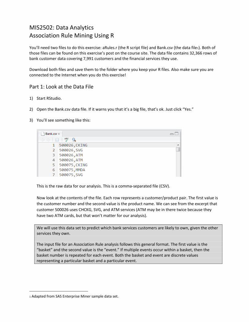
3) You’ll see something like this:

This is the raw data for our analysis. This is a comma-separated file (CSV).

Now look at the contents of the file. Each row represents a customer/product pair. The first value is

the customer number and the second value is the product name. We can see from the excerpt that

customer 500026 uses CHCKG, SVG, and ATM services (ATM may be in there twice because they

have two ATM cards, but that won’t matter for our analysis).

We will use this data set to predict which bank services customers are likely to own, given the other services they own. The input file for an Association Rule analysis follows this general format. The first value is the “basket” and the second value is the “event.” If multiple events occur within a basket, then the basket number is repeated for each event. Both the basket and event are discrete values representing a particular basket and a particular event.

1 Adapted from SAS Enterprise Miner sample data set.

Page 2

For the bank data set, here is the complete list of products and services they offer:

ITEM Description

ATM ATM card

AUTO Auto loan

CCRD Credit card

CD Certificate of deposit

CKCRD Check card

CKING Checking account

HMEQLC Home equity loan

IRA Individual retirement account

MMDA Money market deposit account

MTG Mortgage

PLOAN Personal loan

SVG Savings account

TRUST Trust account

4) Close the Bank.csv file (select) File/Close. If it asks you to save the file, choose “Don’t Save”.

Part 2: Explore the aRules.r Script 1) Open the aRules.r file. This contains the R script that performs the association mining analysis.

The code is heavily commented. If you want to understand how the code works line-by-line you can read the comments. For the purposes of this exercise (and this course), we’re going to assume that it works and just adjust what we need to in order to perform our analysis.

2) Look at lines 8 through 21. These contain the parameters for the decision tree model. Here’s a rundown:

INPUT_FILENAME Bank.csv The data is contained in Bank.csv

OUTPUT_FILENAME ARulesOutput.txt The association rules and their statistics (lift, confidence, support) are output to arules.txt.

SUPPORT_THRESH 0.01 If the support for a rule is below 0.01, it won’t appear in the final list.

CONF_THRESH 0.01 If the confidence for a rule is below 0.01, it won’t appear in the final list.

CONF_THREST_PLOT 0.50 If the confidence for a rule is below 0.50, it won’t appear in the plot. We usually make this higher than CONF_THRESH because a lot of rules makes the plot difficult to read.

3) Look at lines 29 through 33. These install (when needed) the arules and arulesViz packages. These

do the analysis and visualization of the association rules.

Page 3

Part 3: Execute the aRules.r Script 1) Select Session/Set Working Directory/To Source File Location to change the working directory to the

location of your R script.

2) Select Code/Run Region/Run All. It could take a few seconds to run since the first time it has to install some extra modules to do the analysis. Be patient!

3) You’ll see a lot of action in the Console window at the bottom left side of the screen, ending with this:

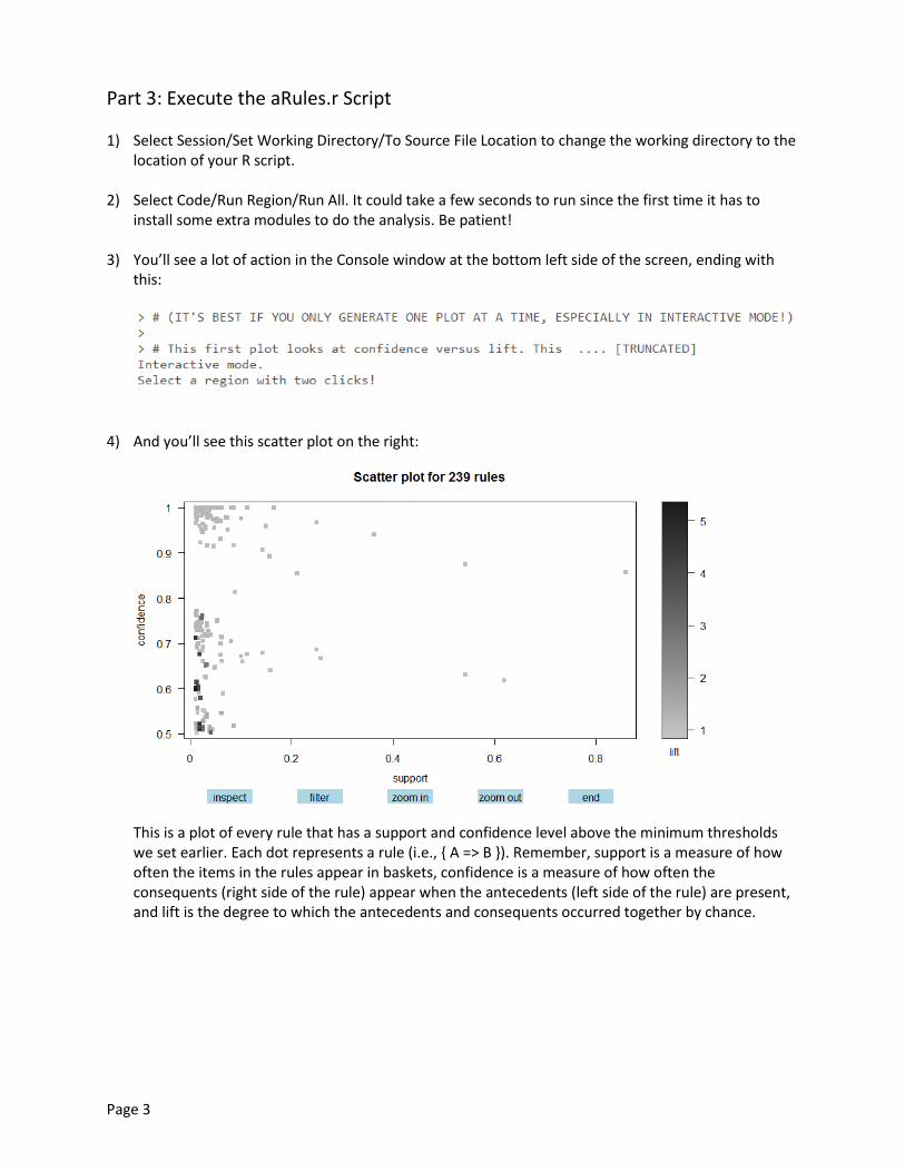
4) And you’ll see this scatter plot on the right:

This is a plot of every rule that has a support and confidence level above the minimum thresholds we set earlier. Each dot represents a rule (i.e., { A => B }). Remember, support is a measure of how often the items in the rules appear in baskets, confidence is a measure of how often the consequents (right side of the rule) appear when the antecedents (left side of the rule) are present, and lift is the degree to which the antecedents and consequents occurred together by chance.

Page 4

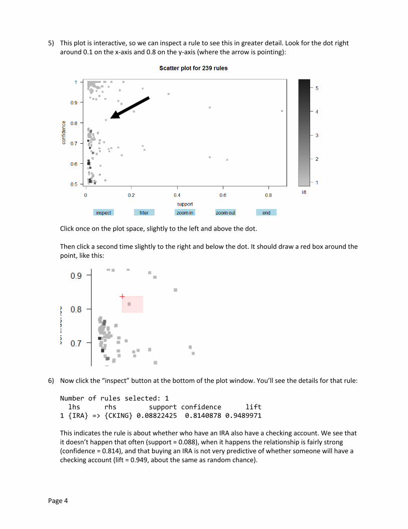
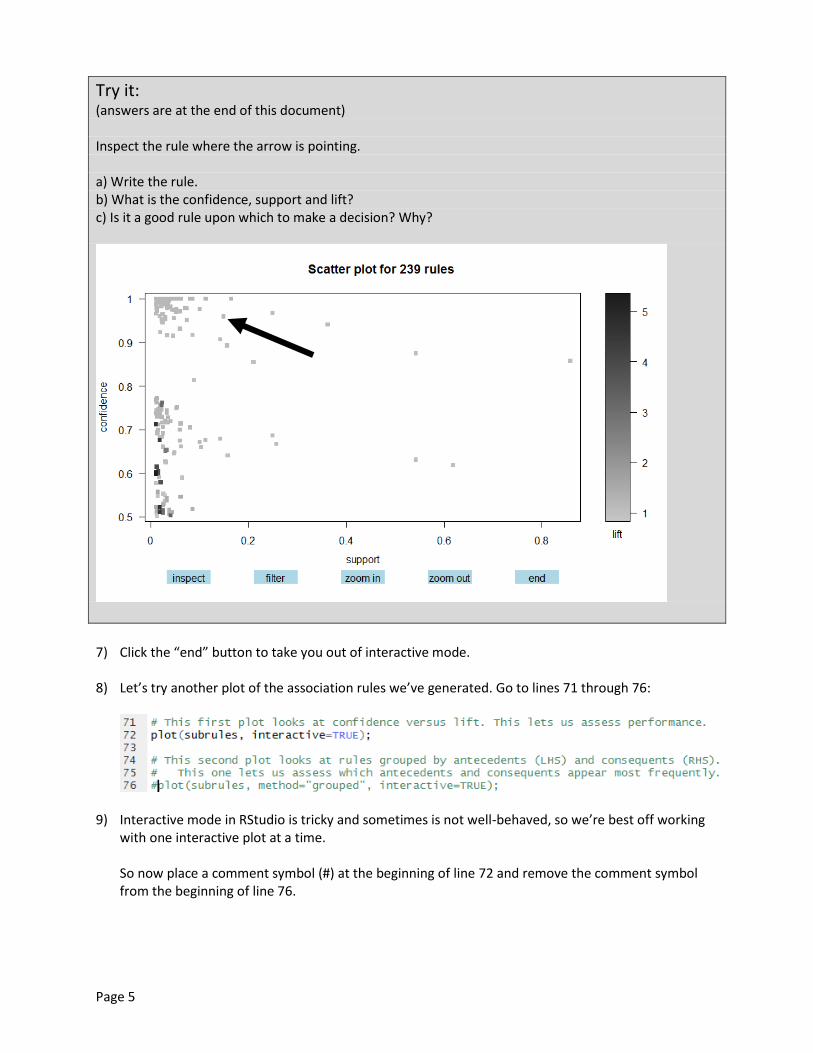
5) This plot is interactive, so we can inspect a rule to see this in greater detail. Look for the dot right around 0.1 on the x-axis and 0.8 on the y-axis (where the arrow is pointing):

Click once on the plot space, slightly to the left and above the dot. Then click a second time slightly to the right and below the dot. It should draw a red box around the point, like this:

6) Now click the “inspect” button at the bottom of the plot window. You’ll see the details for that rule: Number of rules selected: 1 lhs rhs support confidence lift 1 {IRA} => {CKING} 0.08822425 0.8140878 0.9489971 This indicates the rule is about whether who have an IRA also have a checking account. We see that it doesn’t happen that often (support = 0.088), when it happens the relationship is fairly strong (confidence = 0.814), and that buying an IRA is not very predictive of whether someone will have a checking account (lift = 0.949, about the same as random chance).

Page 5

Try it: (answers are at the end of this document) Inspect the rule where the arrow is pointing. a) Write the rule. b) What is the confidence, support and lift? c) Is it a good rule upon which to make a decision? Why?

7) Click the “end” button to take you out of interactive mode.

8) Let’s try another plot of the association rules we’ve generated. Go to lines 71 through 76:

9) Interactive mode in RStudio is tricky and sometimes is not well-behaved, so we’re best off working with one interactive plot at a time. So now place a comment symbol (#) at the beginning of line 72 and remove the comment symbol from the beginning of line 76.

Page 6

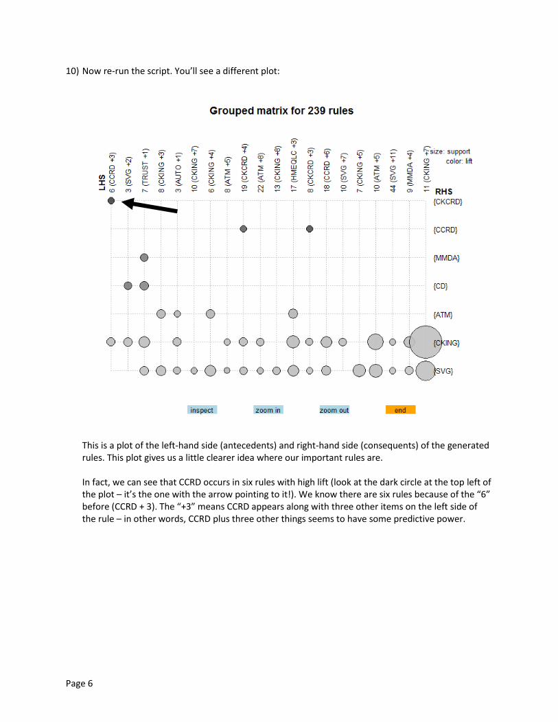
10) Now re-run the script. You’ll see a different plot:

This is a plot of the left-hand side (antecedents) and right-hand side (consequents) of the generated rules. This plot gives us a little clearer idea where our important rules are. In fact, we can see that CCRD occurs in six rules with high lift (look at the dark circle at the top left of the plot – it’s the one with the arrow pointing to it!). We know there are six rules because of the “6” before (CCRD + 3). The “+3” means CCRD appears along with three other items on the left side of the rule – in other words, CCRD plus three other things seems to have some predictive power.

Page 7

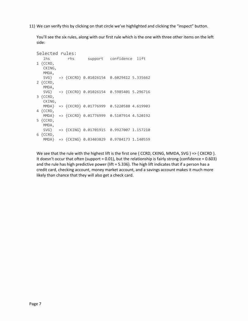
11) We can verify this by clicking on that circle we’ve highlighted and clicking the “inspect” button. You’ll see the six rules, along with our first rule which is the one with three other items on the left side:

Selected rules: lhs rhs support confidence lift 1 {CCRD, CKING, MMDA, SVG} => {CKCRD} 0.01026154 0.6029412 5.335662 2 {CCRD, MMDA, SVG} => {CKCRD} 0.01026154 0.5985401 5.296716 3 {CCRD, CKING, MMDA} => {CKCRD} 0.01776999 0.5220588 4.619903 4 {CCRD, MMDA} => {CKCRD} 0.01776999 0.5107914 4.520192 5 {CCRD, MMDA, SVG} => {CKING} 0.01701915 0.9927007 1.157210 6 {CCRD, MMDA} => {CKING} 0.03403829 0.9784173 1.140559

We see that the rule with the highest lift is the first one { CCRD, CKING, MMDA, SVG } => { CKCRD }. It doesn’t occur that often (support = 0.01), but the relationship is fairly strong (confidence = 0.603) and the rule has high predictive power (lift = 5.336). The high lift indicates that if a person has a credit card, checking account, money market account, and a savings account makes it much more likely than chance that they will also get a check card.

Page 8

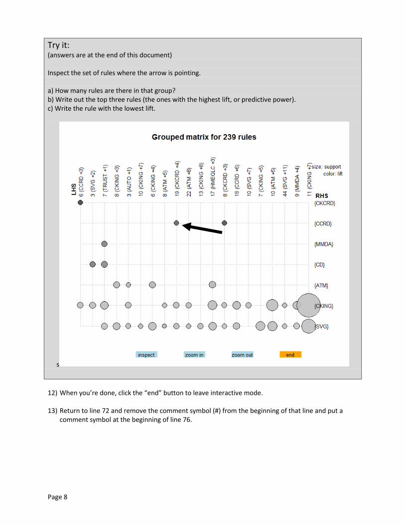
Try it: (answers are at the end of this document) Inspect the set of rules where the arrow is pointing. a) How many rules are there in that group? b) Write out the top three rules (the ones with the highest lift, or predictive power). c) Write the rule with the lowest lift.

s

12) When you’re done, click the “end” button to leave interactive mode.

13) Return to line 72 and remove the comment symbol (#) from the beginning of that line and put a

comment symbol at the beginning of line 76.

Page 9

Part 4: Importing the generated rules into Microsoft Excel for analysis

Working with the interactive plots can be cumbersome and aren’t a very good way to look at all the

rules at once. Fortunately, our aRules script generates an output file listing every rule. The only

restriction is that it won’t include rules with support and confidence levels below the thresholds we set

using SUPPORT_THRESH and CONF_THRESH.

1) Close the aRules.r script. If it asks you to save the file, click “Save.”

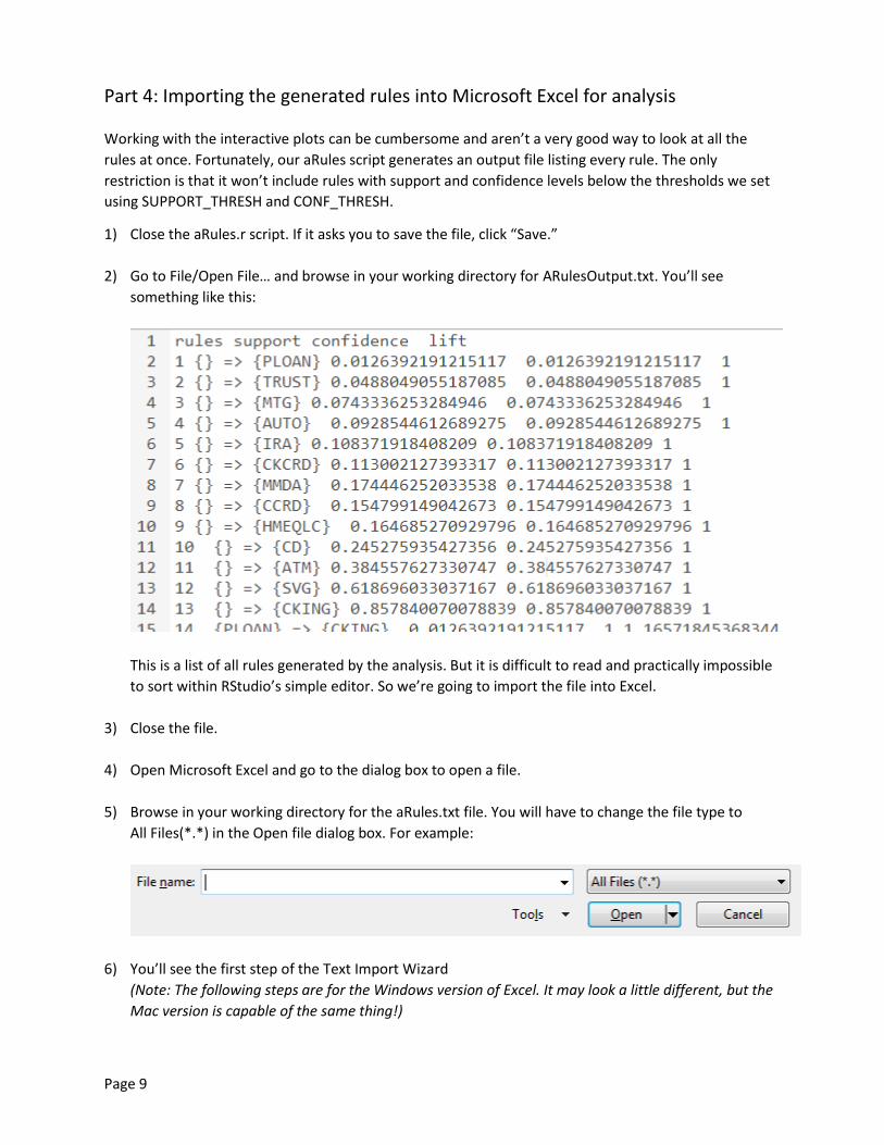
2) Go to File/Open File… and browse in your working directory for ARulesOutput.txt. You’ll see

something like this:

This is a list of all rules generated by the analysis. But it is difficult to read and practically impossible

to sort within RStudio’s simple editor. So we’re going to import the file into Excel.

3) Close the file.

4) Open Microsoft Excel and go to the dialog box to open a file.

5) Browse in your working directory for the aRules.txt file. You will have to change the file type to

All Files(*.*) in the Open file dialog box. For example:

6) You’ll see the first step of the Text Import Wizard

(Note: The following steps are for the Windows version of Excel. It may look a little different, but the

Mac version is capable of the same thing!)

Page 10

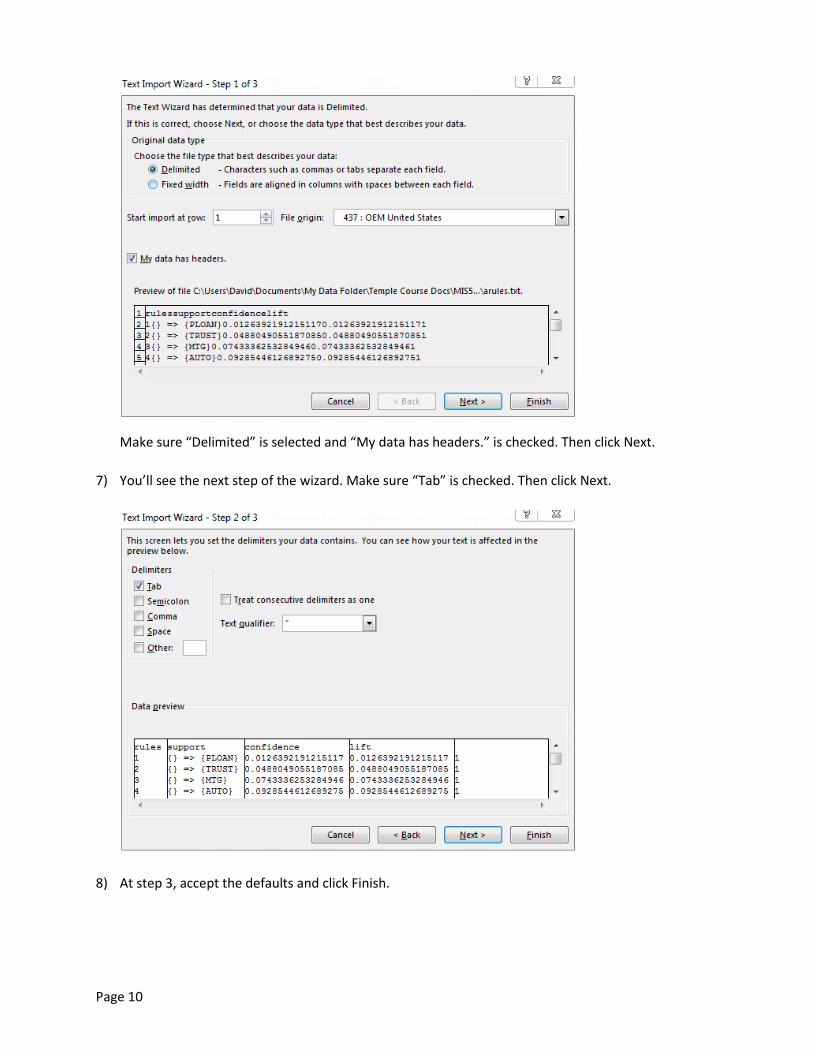
Make sure “Delimited” is selected and “My data has headers.” is checked. Then click Next.

7) You’ll see the next step of the wizard. Make sure “Tab” is checked. Then click Next.

8) At step 3, accept the defaults and click Finish.

Page 11

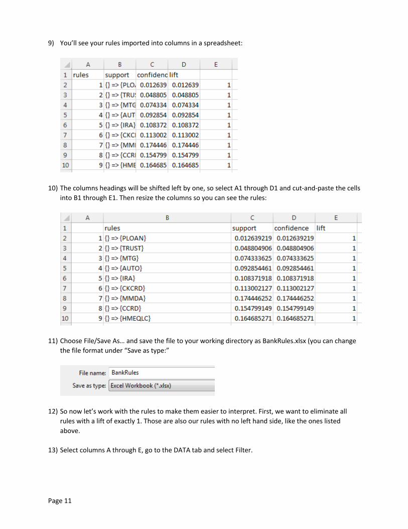
9) You’ll see your rules imported into columns in a spreadsheet:

10) The columns headings will be shifted left by one, so select A1 through D1 and cut-and-paste the cells

into B1 through E1. Then resize the columns so you can see the rules:

11) Choose File/Save As… and save the file to your working directory as BankRules.xlsx (you can change

the file format under “Save as type:”

12) So now let’s work with the rules to make them easier to interpret. First, we want to eliminate all

rules with a lift of exactly 1. Those are also our rules with no left hand side, like the ones listed

above.

13) Select columns A through E, go to the DATA tab and select Filter.

Page 12

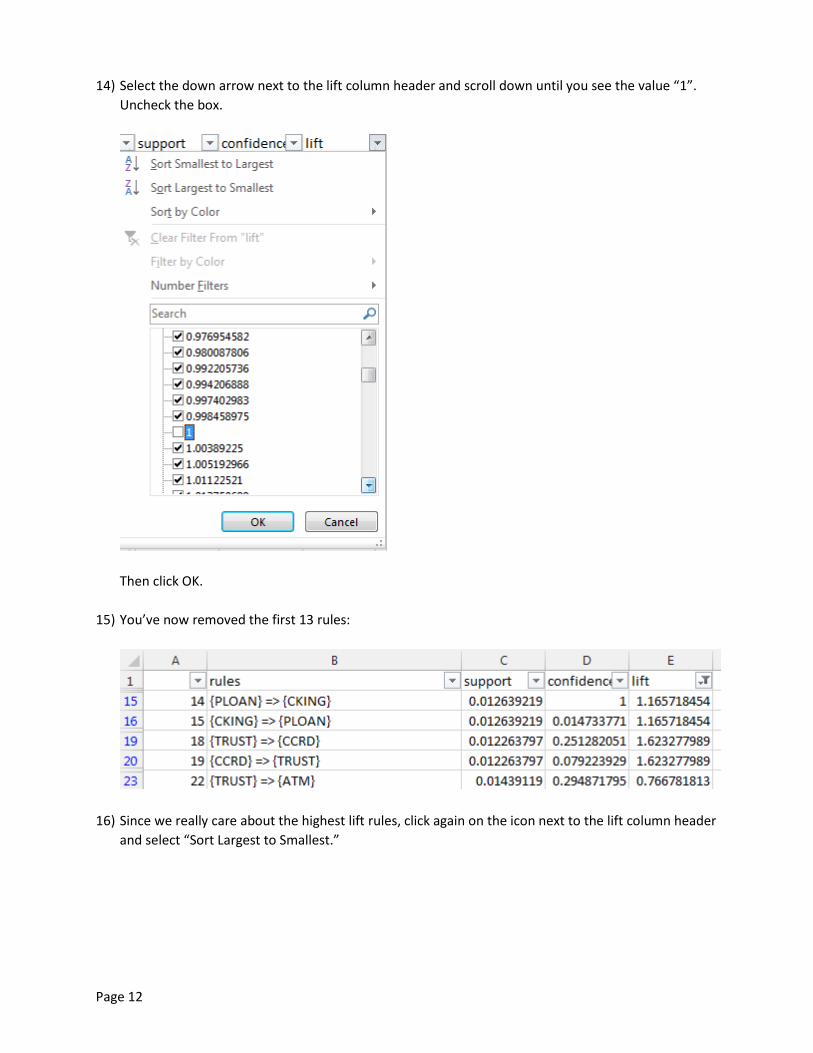
14) Select the down arrow next to the lift column header and scroll down until you see the value “1”.

Uncheck the box.

Then click OK.

15) You’ve now removed the first 13 rules:

16) Since we really care about the highest lift rules, click again on the icon next to the lift column header

and select “Sort Largest to Smallest.”

Page 13

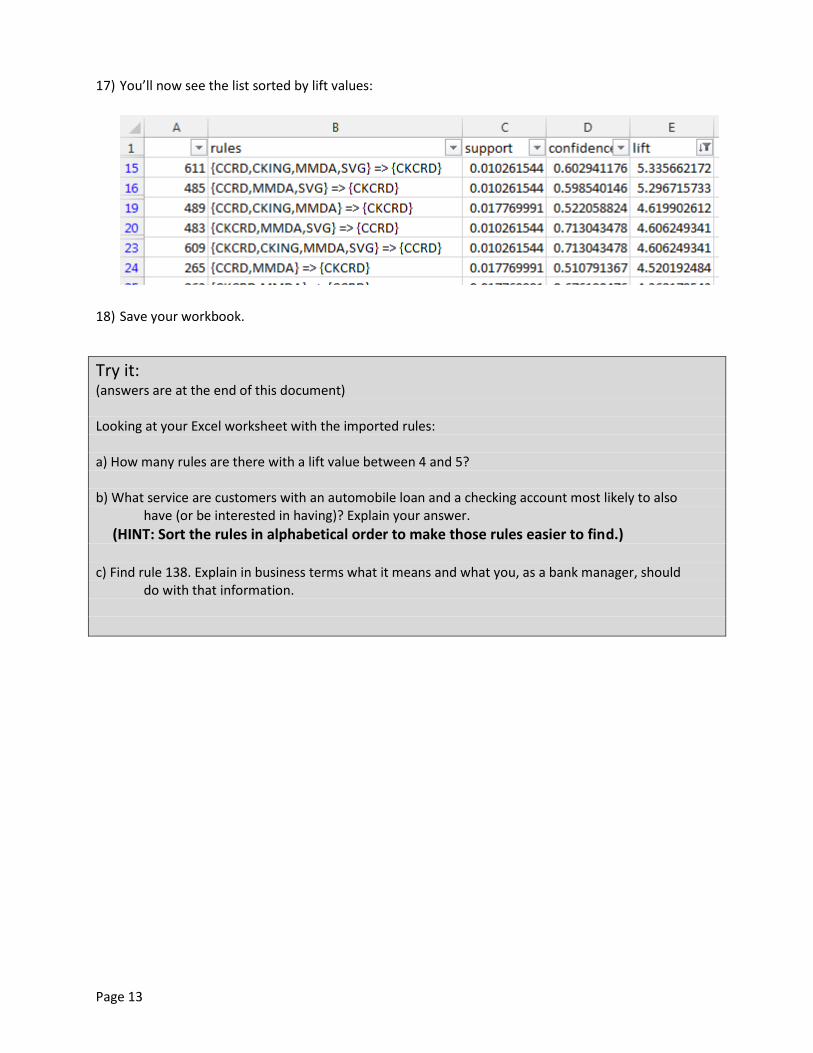
17) You’ll now see the list sorted by lift values:

18) Save your workbook.

Try it: (answers are at the end of this document) Looking at your Excel worksheet with the imported rules: a) How many rules are there with a lift value between 4 and 5? b) What service are customers with an automobile loan and a checking account most likely to also have (or be interested in having)? Explain your answer.

(HINT: Sort the rules in alphabetical order to make those rules easier to find.) c) Find rule 138. Explain in business terms what it means and what you, as a bank manager, should do with that information.

Page 14

Answer Key

Try it on page 5: a) Rule: {CCRD} => {CKING} b) Confidence = 0.960

Support = 0.149 Lift = 1.119

c) Yes, you could make a decision based on this rule. It is more predictive than random chance as lift is greater than 1, and has a high confidence. Support is low, but most of the values for support in this set are relatively low.

Output from R: Number of rules selected: 1 lhs rhs support confidence lift 1 {CCRD} => {CKING} 0.1485421 0.9595796 1.1186

Try it on page 8: a) 19 (you can get this right from the plot) b) Rules in this group with highest lift:

{ CD, CKCRD, SVG } => { CCRD } { CD, CKCRD, CKING, SVG } => { CCRD } { CD, CKCRD } => {CCRD}

c) Rule in this group with lowest lift: { CKCRD, CKING, HMEQLC } => { SVG }

Output from R: Selected rules: 1 {CD, CKCRD, SVG} => {CCRD} 0.01201352 0.6153846 3.975375 2 {CD, CKCRD, CKING, SVG} => {CCRD} 0.01201352 0.6153846 3.975375 3 {CD, CKCRD} => {CCRD} 0.01576774 0.6057692 3.913259 19 {CKCRD, CKING, HMEQLC} => {SVG} 0.02440245 0.7065217 1.141953

Page 15

Try it on page 13: a) 6

b) A home equity loan.

{AUTO, CKING } => {HMEQLC } has the highest lift (1.80). It also has a moderate level of confidence (0.297). This means that it isn’t a strong relationship, but it does occur more often than random chance (so we can rule out coincidence).

c) Rule: { SVG, TRUST } => { CD } The lift is 3.108 and the confidence is also high (0.762). This implies a strong relationship that is also predictive (more likely than random chance). This means that customers who have a savings account and a trust account are also likely to have or want a certificate of deposit. As a bank manager, we could target these customers with a campaign highlighting CDs as an investment opportunity.