Embed Size (px)
Citation preview

MISSILE GUIDANCE WITH IMPACT ANGLE CONSTRAINT
A THESIS SUBMITTED TO THE GRADUATE SCHOOL OF NATURAL AND APPLIED SCIENCES
OF MIDDLE EAST TECHNICAL UNIVERSITY
BY
BARKAN ÇĐLEK
IN PARTIAL FULFILLMENT OF THE REQUIREMENTS FOR
THE DEGREE OF MASTER OF SCIENCE IN
AEROSPACE ENGINEERING
DECEMBER 2014

ii

iii
Approval of the thesis:
MISSILE GUIDANCE WITH IMPACT ANGLE CONSTRAINT
submitted by BARKAN ÇĐLEK in partial fulfillment of the requirements for the degree of Master of Science in Aerospace Engineering Department, Middle East Technical University by, Prof. Dr. Gülbin Dural Ünver __________ Dean, Graduate School of Natural and Applied Sciences Prof. Dr. Ozan Tekinalp __________ Head of Department, Aerospace Engineering Assist. Prof. Dr. Ali Türker Kutay __________ Supervisor, Aerospace Engineering Dept., METU Examining Committee Members: Prof. Dr. Ozan Tekinalp ____________ Aerospace Engineering Dept., METU Asst. Prof. Dr. Ali Türker Kutay ___________ Aerospace Engineering Dept., METU Assoc. Prof. Dr. Đlkay Yavrucuk ____________ Aerospace Engineering Dept., METU Prof. Dr. Kemal Leblebicioğlu ____________ Electrical and Electronics Engineering Dept., METU Prof. Dr. Kemal Özgören ____________ Mechanical Engineering Dept., METU
Date: _____________

iv
I hereby declare that all information in this document has been obtained and
presented in accordance with academic rules and ethical conduct. I also declare
that, as required by these rules and conduct, I have fully cited and referenced
all material and results that are not original to this work.
Name, Last name: Barkan ÇĐLEK
Signature :

v
ABSTRACT
MISSILE GUIDANCE WITH IMPACT ANGLE CONSTRAINT
Çilek, Barkan
M.S., Department of Aerospace Engineering
Supervisor: Assist. Prof. Dr. Ali Türker Kutay
December 2014, 100 Pages
Missile flight control systems are the brains of missiles. One key element of a missile
FCS is the guidance module. It basically generates the necessary command inputs to
the autopilot.
Guidance algorithm selection depends on the purpose of the corresponding missile
type. In this thesis, missile guidance design problem with impact angle constraint is
studied which is the main concern of anti-tank and anti-ship missiles. Different
algorithms existing in the literature have been investigated using various analysis
techniques some of which are not present in the literature.
For the algorithms that need time-to-go information, sensitivity of the algorithm to
the errors in time-to-go measurement is analyzed. In this context, apart from the
time-to-go methods that are used in corresponding algorithms, a different time-to-go

vi
method[1] is employed and sensitivity analysis is repeated. Results with different
time-to-go methods are compared.
Keywords: Impact Angle, Missile Guidance, Launch Envelope, Optimal Guidance,
Proportional Guidance, Time-to-Go

vii
ÖZ
VURUŞ AÇISI KISITLI FÜZE GÜDÜMÜ
Çilek, Barkan
Yüksek Lisans, Havacılık ve Uzay Mühendisliği Bölümü
Tez Yöneticisi:Yrd. Doç. Dr. Ali Türker Kutay
Aralık 2014, 100 Sayfa
Füze uçuş kontrol sistemleri (UKS) füzelerin beyinleridir. Bir füze UKS’sinin önemli
bir parametresi güdüm modulüdür. Bu modül oto-pilotun girdi olarak alacağı gerekli
komutları üretir.
Güdüm algoritması seçimi ilgili füzenin tipine bağlıdır. Bu tezde, daha çok anti-tank
ve anti-gemi füzelerinin bir problemi olan vuruş açısı kısıtına göre güdüm tasarımı
problemi çalışılmıştır. Literatürde var olan algoritmalar bazıları literatürde var
olmayan çeşitli analiz teknikleri kullanılarak incelenmiştir.
Kalan zaman bilgisine ihtiyaç duyan algoritmalar için kalan zaman hesaplamasındaki
hataların başarıma etkisi incelenmiştir. Bu kapsamda, ilgili algoritmalardaki vuruşa
kalan zaman bilgisinden farklı olarak, farklı bir kalan zaman hesaplama[1] yöntemi

viii
uygulanmış ve başarım analizi tekrar edilmiştir. Farklı kalan zaman hesaplama
yöntemiyle olan analizler karşılaştırılmıştır.
Anahtar Kelimeler: Vuruş Açısı, Füze Güdümü, Atış Zarfı, Optimal Güdüm,
Doğrusal Güdüm, Vuruşa Kalan Zaman

ix
Beni sevgiyle büyüten anneme;
Ve beni her zaman destekleyen kardeşime.

x
ACKNOWLEDGEMENTS
I would like to express my sincere appreciation to my supervisor Asst. Prof. Dr. Ali
Türker KUTAY for his valuable suggestions, guidance and support throughout the
thesis.

xi
TABLE OF CONTENT
ABSTRACT ................................................................................................................. v
ÖZ .............................................................................................................................. vii
ACKNOWLEDGEMENTS ......................................................................................... x
TABLE OF CONTENT .............................................................................................. xi
LIST OF FIGURES ................................................................................................... xv
LIST OF TABLES .................................................................................................. xviii
LIST OF SYMBOLS ................................................................................................. xx
CHAPTERS
1 INTRODUCTION ................................................................................................ 1
1.1. Missiles Overview ......................................................................................... 1
1.1.1 Anti-Tank Missiles ................................................................................. 1
1.1.2 Anti-Ship Missiles .................................................................................. 3
1.2. Missile Flight Control System Components ................................................. 5
1.3. Motivation and Purpose of the Work ............................................................ 6
1.4. Scope and Contributions of the Work ........................................................... 6
1.5. Outline ........................................................................................................... 6
2 GUIDANCE WITH IMPACT ANGLE CONSTRAINT: A LITERATURE
SURVEY ...................................................................................................................... 7
2.1. Constraint Definition ..................................................................................... 7
2.2 PN Based Impact Angle Algorithms ............................................................. 7
2.2.1 Biased PN Based Impact Angle Algorithms for Stationary Targets ...... 9

xii
2.2.2 Biased PN Based Impact Angle Algorithms for Non-Stationary Targets
10
2.3 Optimal Control Theory Based Impact Angle Algorithms ......................... 11
2.3.1 Optimal Control Theory Based Impact Angle Algorithms for Stationary
Targets 12
2.3.2 Optimal Control Theory Based Impact Angle Algorithms for Non-
Stationary Targets ............................................................................................... 15
3 GUIDANCE ALGORITHMS MATHEMATICAL ANALYSIS ...................... 17
3.1 PNG Algorithms Detailed Analysis ............................................................ 19
3.1.1 PNG Characteristics without A Bias Term .......................................... 19
3.2 Biased PNG Algorithms Detailed Analysis ................................................ 21
3.2.1 Indirect Impact-Angle-Control Against Stationary Targets Using
Biased Pure Proportional Navigation(IACBPPN)[13] ....................................... 21
3.2.2 Bias Shaping Method for Biased Proportional Navigation with
Terminal Impact Angle Constraint(BSBPN)[15] ............................................... 22
3.2.3 Orientation Guidance (OG) [19] .......................................................... 25
3.3 Optimal Control Theory Based Algorithms Detailed Analysis ................... 28
3.3.1 Generalized Vector Explicit Guidance(GENEX)[31] .......................... 28
3.3.2 State Dependent Riccati Equation Based Guidance Law for Impact
Angle Constrained Trajectories(SDREGL)[27] ................................................. 31
4 SIMULATION.................................................................................................... 35
4.1 Stationary Target ......................................................................................... 35
4.1.1 Run Type I ........................................................................................... 35
4.1.1.1 Simulation with Gravity ON for Stationary Target ...................... 39
4.1.2 Run Type II .......................................................................................... 40
4.1.2.1 Discrete TGH Region ................................................................... 40
4.1.2.2 Miss Distance Contours ................................................................ 43

xiii
4.1.2.3 Cost Function Contours ................................................................ 46
4.1.3 Run Type III ......................................................................................... 49
4.1.3.1 BSBPN Success Investigation ...................................................... 49
4.1.3.2 IACBPPN Success Investigation .................................................. 50
4.1.3.3 GENEX Success Investigation ..................................................... 52
4.1.3.4 SDREGL Success Investigation ................................................... 53
4.1.3.5 OG Success Investigation ............................................................. 54
4.1.3.6 Comments on Run Type III .......................................................... 55
4.2 Non-Stationary Target ................................................................................. 55
4.2.1 Run Type I ........................................................................................... 55
4.2.1.1 Simulation with Gravity ON for Non-Stationary Target .............. 59
4.2.2 Run Type II .......................................................................................... 60
4.2.2.1 Discrete TGH Region ................................................................... 60
4.2.2.2 Miss Distance Contours ................................................................ 61
4.2.2.3 Cost Function Contours ................................................................ 63
4.2.3 Run Type III ......................................................................................... 64
4.2.3.1 GENEX Success Investigation ..................................................... 65
4.2.3.2 OG Success Investigation ............................................................. 65
4.2.3.3 Comments on Run Type III .......................................................... 66
4.2.4 Run Type IV ......................................................................................... 67
4.2.4.1 Run Type IV for Stationary Type Algorithms .............................. 68
4.2.4.2 Run Type IV for Non-Stationary Type Algorithms...................... 70
4.3 Robustness to Time Constant ...................................................................... 71
4.3.1 Robustness to Time Constant Against Stationary Target .................... 71
4.3.2 Robustness to Time Constant Against Non-Stationary Targets ........... 73
4.4 Time-to-Go Error Analysis ......................................................................... 74

xiv
4.4.1 Effect of Additive Term ....................................................................... 75
4.4.1.1 Effects of Additive Terms in the Case of Stationary Target......... 75
4.4.1.2 Effects of Additive Terms in the Case of Non-Stationary Target 77
4.4.2 Effect of Proportional Term ................................................................. 79
4.4.2.1 Effects of Proportional Term in the Case of Stationary Target .... 79
4.4.2.2 Effects of Proportional Terms in the Case of Non-Stationary
Target 80
4.5 Time-to-go Error Analysis with Non-Traditional Time-to-Go Method[1] . 82
4.5.1 Additive Term Varying Case ............................................................... 82
4.5.1.1 GENEX Time-to-go Error Analysis Comparison with New Time-
to-go Method Against Non-Stationary Target ............................................... 82
4.5.1.2 SDREGL Time-to-go Error Analysis Comparison with New Time-
to-go Method against Stationary Target ......................................................... 85
4.5.2 Proportional Term Varying Case ......................................................... 87
4.5.2.1 GENEX Time-to-go Error Analysis Comparison with New Time-
to-go Method Against Non-Stationary Target ............................................... 87
4.5.2.2 SDREGL Time-to-go Error Analysis Comparison with New Time-
to-go Method Against Stationary Target ....................................................... 88
5 CONCLUSIONS AND FUTURE WORK ......................................................... 91
REFERENCES ........................................................................................................... 95
APPENDIX ................................................................................................................ 99

xv
LIST OF FIGURES
FIGURES
Figure 1 Main Battle Tank Components ...................................................................... 2
Figure 2 UMTAS Anti-Tank Missile ........................................................................... 3
Figure 3 MĐLGEM Warship ........................................................................................ 3
Figure 4 Harpoon Missile............................................................................................. 5
Figure 5 Missile Flight Control System ....................................................................... 5
Figure 6 Engagement Schematic for Stationary Target ............................................. 18
Figure 7 Engagement Schematic for a Non Stationary Target .................................. 18
Figure 8 Engagement Schematic (refined) ................................................................. 19
Figure 9 Bias Switching Logic ................................................................................... 23
Figure 10 New Reference Frame for SDREGL ......................................................... 34
Figure 11 Missile Trajectory Histories ...................................................................... 37
Figure 12 Flight Path Angle Histories ....................................................................... 38
Figure 13 Acceleration Histories ............................................................................... 38
Figure 14 Miss Distance Contours for IACBPPN (Stationary) ................................. 44
Figure 15 Miss Distance Contours for IACBPPN (Stationary) ................................. 45
Figure 16 Miss Distance Contours for OG (Stationary) ............................................ 45
Figure 17 Miss Distance Contours for SDREGL (Stationary) .................................. 46
Figure 18 Cost Function Contours for IACBPPN (stationary) .................................. 47
Figure 19 Cost Function Contours for GENEX (stationary) ..................................... 47
Figure 20 Cost Function Contours for OG (stationary) ............................................. 48
Figure 21 Cost Function Contours for SDREGL (stationary) ................................... 48
xvi
Figure 22 Missile Trajectory for Different TGH Orientation .................................... 50
Figure 23 Missile Trajectory History for Various TGH Orientation (IACBPPN) .... 51
Figure 24 Missile Trajectory History for Various TGH Orientation (GENEX) ........ 52
Figure 25 Missile Trajectories for Various TGH Angles (SDREGL) ....................... 53
Figure 26 Missile Trajectories for Various TGH Angles (OG) ................................. 54
Figure 27 Missile Trajectory Histories ...................................................................... 57
Figure 28 Flight Path Angle Histories ....................................................................... 57
Figure 29 Acceleration Histories ............................................................................... 58
Figure 30 Miss Distance Contours for GENEX (non-stationary) .............................. 62
Figure 31 Miss Distance Contours for OG (non-stationary) ...................................... 62
Figure 32 Cost Function Contours for GENEX (non-stationary) .............................. 63
Figure 33 Cost Function Contours for OG (non-stationary) ...................................... 63
Figure 34 Missile Trajectory for Various TGH Angles ............................................. 65
Figure 35 Missile Trajectory for TGH Angles ........................................................... 66
Figure 36 Scatter Graph for BSBPN .......................................................................... 68
Figure 37 Scatter Graph for IACBPPN ...................................................................... 68
Figure 38 Scatter Graph for SDREGL ....................................................................... 69
Figure 39 Scatter Graph for GENEX ......................................................................... 70
Figure 40 Scatter Graph for OG ................................................................................. 70
Figure 41 Miss Distance vs. Time Constant (stationary target) ................................. 71
Figure 42 Impact Angle Error vs. Time Constant (stationary target) ........................ 72
Figure 43 Miss Distance vs. Time Constant (non-stationary target) ......................... 73
Figure 44 Impact Angle vs. Time Constant (non-stationary target) .......................... 74
Figure 45 Miss Distance Error due to Time to go Error (additive/ stationary target) 76
Figure 46 Impact Angle Error due to Time to go Error (additive/ stationary target). 76
Figure 47 Miss Distance Error due to Time to go Error (additive/non-stationary
target) ......................................................................................................................... 78
Figure 48 Impact Angle Error due to Time to go Error (additive/ non-stationary
target) ......................................................................................................................... 78
Figure 49 Miss Distance Error due to Time to go Error (proportional/stationary) .... 79
Figure 50 Impact Angle Error due to Time to go Error (proportional/stationary) ..... 80

xvii
Figure 51 Miss Distance Error due to Time to go Error (proportional/non-stationary)
.................................................................................................................................... 81
Figure 52 Impact Angle Error due to Time to go Error (proportional /non-stationary)
.................................................................................................................................... 81
Figure 53 Miss Distance Error due to Time to go Error (additive/non-stationary) ... 84
Figure 54 Impact Angle Error due to Time to go Error (additive/non-stationary) .... 84
Figure 55 Miss Distance Error due to Time to go Error (additive/stationary) ........... 86
Figure 56 Impact Angle Error due to Time to go Error (additive/stationary) ............ 86
Figure 57 Miss Distance Error due to Time to go Error (proportional/non-stationary)
.................................................................................................................................... 87
Figure 58 Impact Angle Error due to Time to go Error (proportional/non-stationary)
.................................................................................................................................... 88
Figure 59 Miss Distance Error due to Time to go Error (proportional/ stationary) ... 89
Figure 60 Impact Angle Error due to Time to go Error (proportional/ stationary) .... 89

xviii
LIST OF TABLES
TABLES
Table 1 Scenario I Run I Parameters.......................................................................... 36
Table 2 Scenario I Run I Results ............................................................................... 39
Table 3 Simulation Properties With Gravity for Stationary Target ........................... 39
Table 4 Results with Gravity for Stationary Target ................................................... 40
Table 5 Scenario I Run II Parameters ........................................................................ 41
Table 6 BSBPN Launch Envelope for Non-Accelerating Missile against Stationary
Target ......................................................................................................................... 42
Table 7 IACBPPN Launch Envelope for Non-Accelerating Missile against Stationary
Target ......................................................................................................................... 42
Table 8 GENEX Launch Envelope for Non-Accelerating Missile against Stationary
Target ......................................................................................................................... 42
Table 9 SDREGL Launch Envelope for Non-Accelerating Missile against Stationary
Target ......................................................................................................................... 43
Table 10 OG Launch Envelope for Non-Accelerating Missile against Stationary
Target ......................................................................................................................... 43
Table 11 Simulation Properties .................................................................................. 43
Table 12 TGH Angle Test Points ............................................................................... 49
Table 13 Success Chart of BSBPN for Various TGH Orientation ............................ 50
Table 14 Success Chart of IACBPPN for Various TGH Orientation ........................ 51
Table 15 Success Chart of GENEX for Various TGH Angles .................................. 52
Table 16 Success Chart of SDREGL for Various TGH Angles ................................ 54
Table 17 Success Chart of OG for Various TGH Angles .......................................... 55
Table 18 Scenario II Run I Parameters ...................................................................... 56
Table 19 Scenario II Run I Results ............................................................................ 58

xix
Table 20 Simulation Parameters for Non-Stationary Targets with Gravity ............... 59
Table 21 Results with Gravity for Non-Stationary Target ......................................... 59
Table 22 Scenario II Run II Parameters ..................................................................... 60
Table 23 GENEX Launch Envelope for Non-Accelerating Missile against Non-
Stationary Target ........................................................................................................ 61
Table 24 OG Launch Envelope for Non-Accelerating Missile against Non-Stationary
Target ......................................................................................................................... 61
Table 25 Simulation Properties .................................................................................. 61
Table 26 TGH Test Points ......................................................................................... 64
Table 27 Success Chart of GENEX for TGH Angles (non-stationary target) ........... 65
Table 28 Success Chart of GENEX for Various TGH Angles (non-stationary target)
.................................................................................................................................... 66
Table 29 Scenario II Run IV Parameters ................................................................... 67
Table 30 Simulation Parameters ................................................................................ 75
Table 31 Simulation Parameters ................................................................................ 77
Table 32 Simulation Parameters ................................................................................ 82
Table 33 Summary of Merits of Performance............................................................ 91
Table 34 Time-to-go Formulas ................................................................................ 100

xx
LIST OF SYMBOLS
� Angle of Attack
�� Flight Path Angle
� Line of Sight Angle
�� Missile Final Flight Path Angle
��� Initial Firing Angle
�� Target Flight Path Angle
��� Impact Angle
�� Desired Impact Angle
� Missile Look Angle
� Target Look Angle
Time-to-Go
UKS Uçuş Kontrol Sistemi (Flight Control System)
LOS Line of Sight
FCS Flight Control System
MCLOS Manuel Commanded Line of Sight
SACLOS Semi-Automatic Command to Line of Sight
IIR Imaging Infrared

xxi
LADAR Laser Detection and Ranging
IMU Inertial Measurement Unit
CIWS Closed in Weapon System
PNG Proportional Navigation Guidance
PN Proportional Navigation
PPN Pure Proportional Navigation
TPN True Proportional Navigation
BPN Biased Proportional Navigation
BPPN Biased Pure Proportional Navigation
ACPNG Angle Constrained Biased Proportional Navigation
BSBPN Biased Shaping Biased Proportional Guidance
IACBPPN Impact Angle Constrained Biased Pure Proportional Guidance
GENEX Generalized Vector Explicit Guidance
SDREGL State Dependent Riccati Equation Guidance Law
OG Orientation Guidance
TGH Terminal Guidance Handover
ZEM Zero Effort Miss
GUI Graphical User Interface
SWIL Software-in-the-Loop

xxii

1
CHAPTER 1
1 INTRODUCTION
1.1. Missiles Overview
In a modern military usage, a missile is a self-propelled guided weapon system, as
opposed to unguided self-propelled munitions, referred to as just a rocket.[2]
Depending upon the purpose, missiles can be classified under four different
categories as follows.
• Surface to Air
• Surface to Surface
• Air to Surface
• Air to Air
In order to have an overview of the missiles that have been produced up to now, one
may refer to [3].
In this study, missile guidance design with impact angle constraint is studied. Impact
angle is important for anti-tank and anti-ship missiles. Before explanation of why
these constraints refer to this type of missiles, anti-tank and anti-ship missiles are
examined briefly in the following sub-sections.
1.1.1 Anti-Tank Missiles
Tanks are important assets to land forces of an army. In land warfare, they are
usually supported by air forces and infantry. The schematic of a main battle tank can
be seen in the picture below.[4]

2
Figure 1 Main Battle Tank Components
Guidance techniques that are employed in anti-tank missiles can be classified under
three different categories which are as following.
• MCLOS
• SACLOS
• Fire and Forget (Homing Guidance)
Missiles’ successes that use MCLOS type of guidance relies hardly upon the
operator’s skill. Because, the operator watches the missile flight, and uses a signaling
system to command the missile back into the straight line between operator and
target (LOS). [5]
In SACLOS type of guidance, target tracking is done by operator manually, however
control and tracking of missile is done automatically. It is easier than MCLOS due to
the fact that operator has to only track the target, not both the missile and the target.
Fire and forget types of missiles are the most advanced of all above. In this type of
guidance, operator only fires the missile and there is no need for illumination or other
external aids thereafter for the missile to hit the target because missile carries laser,
IIR seeker or a radar seeker mounted on the nose of the missile.

3
An anti-tank missile which is produced by ROKETSAN Missile Industries is shown
below. [6]
Figure 2 UMTAS Anti-Tank Missile
1.1.2 Anti-Ship Missiles
There are various types of warships classified according to their usage. A list of them
can be found in [7]. A sample ship picture which is MĐLGEM produced by Istanbul
Military Shipyard is shown below.
Figure 3 MĐLGEM Warship
Anti-ship missile guidance techniques are similar to the anti-tank missiles. The ones
that are used mostly can be classified as following.

4
• MCLOS Guidance
• SACLOS Guidance
• Beam Riding Guidance
• Homing Guidance ( Active, Semi-Active, Passive)
MCLOS and SACLOS guidance was described in the previous sub-section; hence
they are not explained in this chapter.
Beam riding guidance is a form of command guidance. In this type of guidance, the
target is tracked by means of an electromagnetic beam, which may be transmitted by
a ground (or ship or airborne) radar or a laser tracking system (e.g., a LADAR, or
laser radar). [8]
The expression homing guidance is used to describe a missile system that can sense
the target by some means, and then guide itself to the target by sending commands to
its own control surfaces.[8] There are three types of homing guidance. First one is
active homing which means the missile illuminates and tracks the target itself
without an external aid. Second one is semi-active homing in which the missile
tracks the target onboard whereas the target is illuminated by sources outside of the
missile (i.e., ground based illumination radar). Final one is the passive homing. In
this type of guidance, missile relies on natural sources such as light or heat waves for
illumination of the target where tracking is done onboard.
A sample anti-ship missile, Harpoon, produced by McDonell Douglas and Boeing
Defense is displayed below.[9]

1.2. Missile Flight
A missile flight control system structure is given below
Guidance law decides the appropriate commands to be sent to autopilot in order to
reach the desired destination. Autopilot receives the commands from the guidance
5
Figure 4 Harpoon Missile
Flight Control System Components
flight control system structure is given below.[10]
Figure 5 Missile Flight Control System
Guidance law decides the appropriate commands to be sent to autopilot in order to
reach the desired destination. Autopilot receives the commands from the guidance
Guidance law decides the appropriate commands to be sent to autopilot in order to
reach the desired destination. Autopilot receives the commands from the guidance

6
law (i.e., acceleration) and calculates the necessary moving surface deflections
ordered to the actuators. Actuators are the physical connections that transmit the
commands of autopilot to the moving surfaces. Airframe responds the moving
surfaces’ commands by changing the position and orientation of the airframe. IMU
senses these differences for each time step and sends the necessary information to the
autopilot.
1.3. Motivation and Purpose of the Work
In literature, there are numerous papers that study the impact angle problem.
Nonetheless, no thesis work exists that studies these algorithms extensively in a more
systematic manner. Main purpose is to outline these algorithms and analyze 5 of
them in a detailed manner.
1.4. Scope and Contributions of the Work
Scope of the thesis is the guidance algorithms that aim to specify the impact angle
which finds application of anti-ship and anti-tank missiles. Missile is assumed to
have a time constant of 0.25 sec which is modeled with a first order transfer function.
However, there is a section which is devoted to the robustness analysis in order to
see the effects of different time constants.
There are many simulations each of which aims to extract a specific behavior of the
algorithm of interest. TGH orientation analysis, engagement field color-coded graphs
and impact angle variance with respect to different target speeds are new analysis’
that are not present in the literature. Another contribution is the application of a new
time-to-go method [1] which is not used in the algorithms that require time-to-go
information. This new time-to-go method is used in time-to-go error analysis which
shows the errors induced by wrongly estimated/measured time-to-go in reality using
a model from literature.[11]
1.5. Outline
Chapter 2 incorporates the literature survey which is about the guidance algorithms
with impact time constraint. Chapter 3 describes and compares the guidance
algorithms existing in the literature. Chapter 4 presents the simulation results.
Chapter 5 includes the conclusions and future work.

7
CHAPTER 2
2 GUIDANCE WITH IMPACT ANGLE CONSTRAINT: A
LITERATURE SURVEY
2.1. Constraint Definition
Impact angle of a missile to the target is of growing importance in modern warfare.
For instance, in case of wars in urban areas, decreasing the collateral damage may
help degrade the civilian casualties. This can be achieved with a direct vertical attack
to the enemy units. Hence, achieving an impact angle of 90 degrees is of crucial
importance for this case. Second case showing the importance of determining impact
angle is for anti-tank missiles. Tanks have different vulnerability characteristics
depending on the place where they would be hit. Hence, being able to specify the
impact angle stands as a very important advantage. Another situation is the anti-ship
missiles. Modern warfare ships have a variety of defenses against anti-ship missiles
such as CIWS. CIWS is a naval shipboard weapon system for detecting and
destroying incoming anti-ship missiles and enemy aircraft at short range.[12]
Because CIWS covers some fan-shaped zone limited in range and azimuth and
taking advantage of CIWS’ weakness of multi-target engagement, if missiles are
fired in a narrow space in azimuth, chance to destroy the target would increase
dramatically. Techniques to control impact angle will be discussed in the next
section.
2.2 PN Based Impact Angle Algorithms

8
PNG is probably the most popular among all of the guidance methods and vast
amount of literature exists of this guidance law. Simply stating, this law tries to
nullify the LOS(the line vector that connects the positions of the pursuer and the
evader) rate by dictating the pursuer to rotate its velocity vector at a rate that is
proportional to the rotation rate of the LOS. Simple scalar form of this law is given
as :
�� = ��� ���� (1)
an= the commanded normal (or lateral) acceleration in ft/sec2 or m/sec2 N= the navigation constant (also known as navigation ratio, effective navigation ratio and navigation gain), a positive real number (dimensionless) usually between 3-5 Vc= the closing velocity [ft/sec] or [m/sec] (�6��)=the LOS rate measured by the missile seeker[rad/sec]
PPN is one of the forms of proportional navigation. The pursuer issues acceleration
commands perpendicular to its velocity vector. PPN is usually applicable to endo-
atmospheric engagements where control forces are generated by aerodynamic lift,
because we do not have control authority to realize the forward velocity requirement
which is the case with TPN. In TPN, on the contrary, acceleration commands are
perpendicular to instantaneous LOS. It is usually employed in exo-atmospheric
missiles where acceleration commands are realized by thrust vectoring so that
forward velocity component of the acceleration command can be satisfied. Neither of
TPN or PPN can control the impact angle.
Another form of PN is BPN with which impact angle can be controlled. In this type
of navigation, a bias term is added to the proportional navigation term where this bias
term might be a function of many variables.

9
2.2.1 Biased PN Based Impact Angle Algorithms for Stationary Targets
Erer and Merttopçuoğlu [13] used Biased Pure Proportional Navigation (BPPN) to
intercept stationary targets aiming to control the impact angle. In the paper, non-
linear equations representing the BPPN kinematics with a stationary target are solved
in closed form. After that introducing non-dimensional range and time into the non-
linear equations, authors derived a stability criterion which defines the conditions
that the engagement will lead to a capture. What follows is the outline of the two
phase guidance scheme which uses bias action to postpone the rotating of the
pursuer’s velocity vector to target until the bias value is reached. After the bias value
is reached, missile flies with PPN only. It is important to note that only LOS rate is
required to realize this law which corresponds to ease of implementation to the actual
missile.
Jeong et al.[14] proposed a so called angle constrained biased PNG (ACBPNG) law
to control impact angle. The required bias angle is analytically calculated.
Acceleration histories, trajectories and flight path angles of ACBPNG and
conventional PNG are compared. Moreover, maneuverability, anti-detection and
sensitivity to navigational errors are analyzed. In the end, simulations are carried out
to see the variation of vertical distance, commanded acceleration and flight path
angle with respect to initial range, initial vertical distance, impact angle and closing
velocity. Authors underline the reality that this law does not guarantee optimality in
any point of view.
Kim et al.[15] propose a bias shaping method based on the two-phase BPN guidance
which can achieve both terminal angle constraint and look angle limitation to
maintain the seeker lock-on condition with the acceleration capability being limited.
Bias shaping is done on the requirement that the integral of the bias should have the
required value before the interception. Law basically consists of two time-varying
biases and switching logic. The method does not require time-to-go or range
information, only LOS rate is required. Because of these, this law can easily be
implemented on a missile with a passive seeker.

10
Ratnoo and Ghose [16] propose a PNG based guidance law for capturing all possible
impact angles in a surface-to-surface planar engagement against a stationary target.
For the initial phase, an orientation guidance scheme is proposed. After following the
orientation trajectory, missile can switch over to a navigation constant N>=2 to
achieve the desired impact angle. The navigation constant through the orientation
phase changes according to the initial engagement geometry. Simulations are carried
out for constant speed missile model and realistic missile model for which ideal and
first order autopilot cases are considered.
2.2.2 Biased PN Based Impact Angle Algorithms for Non-Stationary Targets
Kim et al.[17] derived a guidance law based on non-linear engagement model. Usage
of nonlinear kinematics made it possible to derive analytic conditions for fulfilling
the guidance law. The new law is a modification of the classical PNG law which
includes a time-varying bias. One important advantage of the proposed guidance law
is that it does not require time to go information which may be corrupted by noise or
estimation errors in reality. Moreover, by comparing an optimal linear law, it is
proved that the proposed law is optimal near collision course provided that constants
in the proposed law are equal to some specific integer values.
Model et al.[18] designed a guidance law named Modified angle constrained biased
proportional navigation guidance (MACBPNG). MACBPNG is capable of achieving
a wide range of impact angles in which the required bias term is derived in a closed
form considering non-linear equations of motion (EOM). The commanded
acceleration is perpendicular to LOS which means this law can be thought as a form
of TPN. Bias term is updated at every iteration to get better accuracy. In the end, the
law is compared with an existing law[14]. It is seen that MACBPNG has a wider
launch envelope than ACBPNG.
Ratnoo and Ghose[19] improved their guidance law for non-stationary non-
maneuvering targets. Similar to the former paper they released, they presented an
orientation scheme for the first phase after which scheme is turned to PNG with N=3.
The navigation constant used in the orientation phase depends on the initial geometry

11
between the target and the interceptor. Simulations are carried out for constant speed
and realistic interceptor models with ideal and 1st order autopilot. Robustness of the
law is verified with this 1st order autopilot model.
Lee et al.[20] examined the effects of system lag on performance of a generalized
impact-angle-control-guidance law, analytic solutions of the proposed guidance law
is derived for a first order system. This analytic solution is obtained by solving a
third order linear time-varying ordinary differential equation. Terminal misses due to
system lag have been investigated using the analytic solutions; the effects of
guidance coefficients on the terminal misses have been discussed.[20] Moreover,
sensitivity of impact angle error and miss distance is analyzed with respect to impact
angle and initial heading angle. Finally, analytic solutions have been compared with
the linear and nonlinear simulations.
Ratnoo and Ghoose [19] improved their first algorithm for non-stationary targets. For
initial phase, orientation guidance is proposed like in [19]. For the initial phase, there
are additional terms like velocity ratio of target and interceptor and interceptor’s
flight path angle. While deriving the orientation guidance constant, zero interceptor
flight path angle is assumed. A proof is also given stating that if the missile can be
brought to point 3 on the orientation trajectory, any impact angle can be achieved
between –π and 0. After that, the proposed guidance law is given concisely in a well-
defined manner. Up to now, constant speed missile is assumed. One more derivation
is given for realistic missile model in which first order autopilot lag is assumed.
Simulations are carried out for both cases.
2.3 Optimal Control Theory Based Impact Angle Algorithms
In some impact angle problems, optimal control theory is used to solve the
constraints imposed on the problem. These problems incorporate a cost function in
which the performance measure of interest exists. This measure may be time to go,
altitude climbed, control effort. For instance, if cost function’s parameter is
acceleration effort squared[21], it is defined as below.

12
: = ; <�=�>� �� (2)
After defining the cost function, it is tried to be minimized using optimal control
algorithms which depend on the problem characteristics. The following papers
present these issues.
2.3.1 Optimal Control Theory Based Impact Angle Algorithms for Stationary
Targets
Kim and Grider [22] published the first paper that discusses the impact angle control
problem. Two problems are defined depending on the auto-pilot lag. First problem
has no autopilot lag where the nonlinear engagement kinematics is expressed in
state-space form. Second problem is defined with auto-pilot lag which is also in
state-space form with nonlinear variables. Cost function is expressed in terms of the
input to the autopilot (fin angle) and the final states of range vector projected on the
ground and body attitude angle. Optimal control is then expressed in terms of state
variables with the gains changing with respect to time. Effects of “soft” and “hard”
constraints on acceleration were shown. Finally, initial states for which the miss
distance and attitude angle at impact are satisfactory are extracted by solving the
equations backward in time.
Ryoo et al.[1] generalized optimal guidance laws specifying impact angle and zero
miss distance for arbitrary missile dynamics. The optimal guidance command is
represented by a linear combination of the ramp and the step responses of the
missile’s lateral acceleration. The guidance law is investigated for ideal autopilot and
first order lag autopilot models. New time to go calculation methods are proposed
considering path curvature. In the end, nonlinear and adjoint simulations are carried
out and comparisons are made with biased PN law.[17] It is seen that OGL spends
less control energy than BPN. Moreover, OGL has finite lateral acceleration demand
as the missile approaches the target whereas BPN’s demand shoots up to infinity.
13
Subchan [23] presents some computational results of the optimal trajectory of
missile by minimizing the integrated altitude along the optimal trajectory especially
to avoid increasing anti-missile capability. In order to solve this problem, author first
introduced nonlinear equations of motion of a point mass moving over a flat non-
rotating earth. After that, aerodynamic parameters and constraints are outlined. The
motion is divided into three phases. In the 1st phase interceptor is moving steady and
level. In the 2nd phase it climbs and dives into the target thereafter. Optimization
problem is solved using direct collocation( for more information reader may refer to
[24] ) method. In the end, simulations are carried out and comments are made.
Ryoo et al.[25] proposed a new guidance law based on linear quadratic optimal
control theory with terminal constraints on miss distance and impact angle for a
constant speed missile against a stationary target. Cost function is weighted by a
power of time-to-go. Selection of guidance gains and trajectory shaping are possible
by varying the exponent of the weighting function. An important contribution of this
paper is that it incorporates a new time to go calculation method. Non-linear and
adjoint simulations are made and law is compared with a Biased PNG Law [17]and it
is shown that performance of the new law is better than BPNG law especially in the
terminal homing phase.
Yao et al.[11] derived an energy optimal guidance law aiming to minimize the
control effort and the induced drag which causes velocity loss. The law composes of
two terms one of which representing the proportional navigation term that ensures
impact point accuracy and the other symbolizing the authority on the impact angle. It
is said that the law bases on linearization and small angle assumption. However,
reader cannot see a derivation or any results showing the acceleration demand of the
derived law. Assuming point mass, constant missile velocity and movement in the
vertical plane; authors outlined non-linear equations of motion. Using these
equations, simulations are carried out for large impact angles and it is seen that both
impact point and angle requirements are satisfied. This implies that the guidance law
derived using small angle assumption also works for the large angle cases. Finally,
the error analysis by adding some terms on time to go equation which is assumed that

14
it is calculated by range over closing velocity is done. It turns out to be so that the
closer the interceptor to the target the less the error is calculated.
Lee et al.[26] try to find the feasible set of weighting functions that lead to analytical
forms of weighted guidance laws. Firstly, a cost function is introduced. In the cost
function, there exists an acceleration term squared and a weighting function. The
problem is then started to be solved with linear engagement kinematics. After that
using the Schwarz’s inequality, an optimal acceleration command is derived. This
term includes the weighting function term which is trying to be shaped. A proof is
given saying that any weighting function can provide the analytical form of optimal
solution if up to triple integrations of the inverse of the weighting functions are
analytically given. This is the most important output of this work. In the end of the
paper, using two sample weighting functions acceleration demands are derived.
Ratnoo and Ghose[27] solve the impact angle constrained guidance problem against
a stationary target using the SDRE technique. Firstly, nonlinear engagement
kinematics is outlined and state matrices are formed. Cost function Q is assumed to
be a function of time to go to include the target information in the guidance logic.
After that, an acceleration command is derived. An important thing to note here is
that constant speed assumption is used in the development process. However, in
simulation studies, realistic interceptor model is used with the corresponding
aerodynamic properties. The effect of initial firing angle, impact angle and effect of
guidance parameter N is studied while the other variables being the same in each
simulation. In the end, robustness is studied with respect to autopilot lags and it is
seen that the proposed law shows very low errors for first order delays up to 0.5
seconds.
Park et al.[28] propose a new optimal guidance law considering seeker’s Field of
View (FOV) limits for a missile with a strapdown seeker. The strapdown seeker has
a narrower FOV than that of a gimbaled seeker; hence designer must ensure the FOV
limitations of the missile are not violated during the engagement. In the beginning of
the paper, problem formulation is outlined in which constraints and state equations
are given. After that, using Hamiltonian equations, optimal acceleration commands

15
are derived for initial, midcourse and final phases. In the end, comparison is made
with other existing guidance laws and it is seen that proposed law is more efficient in
terms of control energy.
Lee et al.[29] derived closed-form solutions of an optimal impact-angle-control
guidance against a stationary target for a first-order lag system. First order missile
with constant speed and small flight path angle assumption is made. Based on these
assumptions, mathematical problem is solved by introducing a third order linear time
varying ordinary differential equation. Linear and nonlinear simulations are
performed and the results of them are compared with the analytic solution.
2.3.2 Optimal Control Theory Based Impact Angle Algorithms for Non-
Stationary Targets
Savkin et al.[30] outlined precision missile guidance problem where the successful
intercept criterion has been defined in terms of both minimizing the miss distance
and controlling the missile body attitude with respect to target at the terminal point.
Kinematics are formulated in matrix form, then standard LQR approach and H∞
formulations ( both in state feedback and output feedback form) were used to derive
the optimal control command. Sinusoidal form of maneuvering target model is
considered. It has been shown that H∞ control theory if suitably modified stands as a
powerful tool to solve the precision missile guidance problem.
Ohlmeyer and Phillips[31] propose a new guidance law called generalized vector
explicit guidance (GENEX). Aim of the law is to specify the final missile target
relative orientation called impact angle and make the miss distance zero. A cost
function in terms of time to go and demanded acceleration is introduced with a
weighting factor “n”. Afterwards, using Hamiltonian equations, an acceleration
demand term is derived and the results are applied to proportional navigation. Since
proportional navigation does not specify any final orientation, one more derivation is
done in order to include the impact angle. An advantage of this law is that it is in
vector form which means one can apply this law to 3-dimensional problems. Authors
also reduced the problem to 2-D problem to illustrate the law in single plane. In the

16
end, simulations are carried out for two different scenarios. As a future work, authors
suggested applying this law to higher fidelity weapon models incorporating 6-DOF
dynamics, nonlinear and coupled aerodynamics, and detailed autopilot descriptions.
A new precision guidance law with impact angle constraint for 2-D planar
engagement case is outlined by Manchester and Savkin[32]. In this method, it is
proposed that at every point in space, a different “desired circular path” exists. It is
derived assuming two sets of information, one being restricted than other. For each
set, a different law outcomes. It is compared with a BPNG law in the literature[17]
via simulations for the cases with a limited and unlimited missile acceleration
capability. It is seen that in terms of target speed and the desired impact angle,
proposed law has a wider envelope than that of BPNG. One important advantage of
the proposed law is that it does not require range to target information where all other
impact-angle constrained guidance laws of which the authors are aware require. Final
thing that should be noted is that this law does not claim any optimality in the sense
of acceleration energy where BPNG is nearly optimal in this sense when the missile
starts to close to the collision course.
In this paper, Yoon[33] introduced a circular reference curve on a moving frame
fixed to the target. Using the Frenet formulas, RCNG law for the impact angle
control problem is developed. It is theoretically shown that the proposed law can
solve the impact angle control problem for virtually any initial arrangement of
pursuer and target and any desired impact angle. Moreover, a bound of impact angle
errors under the RCNG law was derived. The proposed law is compared with [32]
and [17]. The 3-D version of this law is available.[34]
17
CHAPTER 3
3 GUIDANCE ALGORITHMS MATHEMATICAL ANALYSIS
Some of the guidance laws outlined in previous chapter will be discussed and
analyzed in more detail in this chapter. In all laws, 2-D engagement will be assumed.
Following engagement geometry for stationary targets and non-stationary targets will
be employed respectively.

18
Figure 6 Engagement Schematic for Stationary Target
Figure 7 Engagement Schematic for a Non Stationary Target

19
Figure 8 Engagement Schematic (refined)
3.1 PNG Algorithms Detailed Analysis
PNG without a bias term cannot control the impact angle. Hence, bias is added to the
PNG algorithms generally to gain the freedom to specify the impact angle before the
engagement. There are some algorithms developed in the literature to this end. They
differ in the sense of choosing the bias and shaping the bias during the engagement.
One may take the seeker gimbal angle limits, physical acceleration limits, fin
actuator rates etc. into account while shaping the bias.
3.1.1 PNG Characteristics without A Bias Term
In this thesis, planar interception problem is studied. Hence, 3-D PNG law will not
be explained here. Interested readers may refer to [35] for a complete 3-D PNG law
derivation.
As stated in the previous section, there are two main forms of PNG law. One is true
proportional navigation guidance and the other is pure proportional navigation
guidance. Neither of these two laws can control the impact angle of which the

20
interceptor missile hits the target. Hence, the impact angle is arbitrary in these laws.
However, it is useful to investigate the characteristics of PNG law. Because, some
forms of optimal control based guidance laws and all forms of biased PNG laws
make use of some of the properties of PNG laws, especially the navigation constant
plays an important role. Not all navigation constants result in a satisfactory
performance in terms of miss distance. The main problem is the saturation of the
commanded acceleration in the final moments. For navigation constants N≥2, there
exists finite commanded acceleration near the interception.[8] Thus, one must choose
a navigation constant equal to or greater than 2 in order to achieve the intercept.
In TPNG or PPNG, there exists a navigation constant that is optimal in terms of
energy spent. The cost function is described as[36]:
J = 12 Cy=(tB) + ;(aD=(t))dtEF� (3)
The optimal control problem aims to find aD that minimizes the functional (3). For
engagement schematic used in this thesis y can be replaced by z which is altitude.
Using optimal control techniques, the solution comes out to be[36]:
aD(t) = 3τ3 CH + τI (z(t) + zK(t)τ) (4)
In order to have zero miss distance, C must go to infinity. Thus, optimal guidance
law becomes:
aD(t) = 3τ= (z(t) + zK(t)τ) (5)
If linear approximation is used,
λ = z RH where R ≅ VOPτ (6)
Taking the derivative of (6);
λK (t) = zK(t)r(t) + z(t)VOPr= = zK(t)τ + z(t)VOPτ= (7)
Inserting (7) to (5);
aD(t) = 3VOPλK (t) (8)
Equation (8) is analogous to equation (1) in which N is replaced by 3. This means
that optimal navigation gain in PNG laws is 3 in the sense of energy used. It is

21
important to note that when the navigation gain is higher than 3, heading error which
is defined as the angle deviation from the collision course can be removed more
quickly than that with 3. However, in that case the effects of guidance noise
associated with λK (t) becomes more significant.[8]
3.2 Biased PNG Algorithms Detailed Analysis
Bias is added to the PNG algorithms generally to gain the freedom to specify the
impact angle before the engagement. There are some algorithms developed in the
literature to this end. They differ in the sense of choosing the bias and shaping the
bias during the engagement. One may take the seeker gimbal angle limits, physical
acceleration limits, fin actuator rates etc. into account while shaping the bias.
3.2.1 Indirect Impact-Angle-Control Against Stationary Targets Using Biased
Pure Proportional Navigation(IACBPPN)[13]
Erer and Merttopçuoğlu’s paper [13] can be summarized as following.
�� = ���K� (9)
To control the impact angle, one may add a bias term as following;
�K� = ��K + Q (10)
Plugging equation (10) into (9), one may get;
�� = ��(��K + QR�S) (11)
If ideal autopilot is assumed, commanded acceleration (�� ) is equal to missile
acceleration (am).
Look angle should be zero at the instant of impact to have the desired impact angle.
Thus, integrating equation (11) and setting −�� = −�� yields the following:
�� = ��U − ��� − V Q���>�W� − 1 (12)

22
In order to have the desired impact angle �� , the bias profile should be selected
accordingly. This profile can be anything including intervals of zero value. However,
a systematic approach should be taken to satisfy the desired impact angle. Two
different approaches are proposed. First approach which is more convenient is as
follows.
Bias is applied till the value �� is equal to desired impact angle. The missile flies
with PPN thereafter. The bias application time should be less than total engagement
time, hence setting it to range over closing velocity (or missile velocity) guarantees
this. Moreover, setting ��to �� , equation (12) can be manipulated to find the initial
bias value as follows.
QU = ��U − ��� − (� − 1)��XU YUH (13)
In order to eliminate the adverse effects of velocity change, velocity weighting is
proposed as following:
Q = QU ∗ YYU (14)
Second approach is to use a full biasing tactic until the impact. This is not a realistic
choice since the successful bias value can be only found by trial and error.
3.2.2 Bias Shaping Method for Biased Proportional Navigation with Terminal
Impact Angle Constraint(BSBPN)[15]
In two phase guidance schemes proposed, in both [13], [15] only LOS rate
information is required which enables these guidance laws’ application to passive
homing missiles. However, in these papers, acceleration capabilities and look angle
limits of the missile are not included in bias design.
BPN guidance can be simply stated as:
�� = ��(��K� + QR�S) (15)
where �K� = ��K� + QR�S
Integrating �K� ; �(�) = ��� + ��(�) + ; Q�
� �� (16)

23
In the case of successful interception of the target with the desired impact angle, look
angle is zero. In this case �� = ��. Then one can have;
; Q�� = (1 − �)��� − ����>
� (17)
Up to this point, Erer and Merttopçuoğlu’s paper[13] was summarized. In this
paper[15], a different bias shaping method is proposed which can provide a
continuous guidance command near the target as well as satisfy the look-angle limit
to maintain the seeker lock-on condition. In this paper, angle of attack is considered
to be small, hence look angle is equal to gimbal angle.
Proposed bias shaping method can be summarized with the following figure. [15]
Figure 9 Bias Switching Logic
In the figure above, RHS of equation (3) is actually equation (17) in this thesis. The
first, b1, is the time varying bias calculated by the difference between the required
integral value, \X]^ = (1 − �)�� − ��, and the integral of bias, B. The second time-
varying bias, b2, is to maintain the constant look (gimbal) angle, which is used if the
look angle approaches the maximum look-angle limit �_`. The switching logic is to
decide which one of the two biases is used to generate the guidance command. In
order to understand the concept better, two different cases are outlined.
Case 1: Assume 0 < � < �_` for the initial moment and look angle (gimbal
angle) does not violate the limits of gimbal angle. For this case, b=b1 and is
exponentially varied as:

24
Q(�) = \de� ]f�g (18)
Taking the integral:
\(�) = ; Q�� = (1 − ]f�g )\de��� (19)
In order to satisfy the impact angle constraint, \ should reach \de� before the
interception of the target, thus should be sufficiently small. It is important to note
that; if ≤ dijk, \ ≅ 0.999\de�for � ≥ 7 since the length of the curved trajectory for
the impact angle control is larger than the straight line which is initial range X� .
Another aspect is that one should put a bound on Qo to keep the guidance command
within the acceleration limit ��_` because a large bias may be produced owing to the
difference between \ and \de� in the initial homing phase. Hence Qo,�_` = _pqrs is
implemented.
Case 2: Being same with the Case 1, 0 < � < �_` for launching moment however
for this case, || > �_` occur at a time during engagement. This means that desired
impact angle is greater than that of case 1. For this case, Q = Qois initially used.
However, when || > �_` occurs, bias is switched to Q = Q= = (1 − �)�K to
maintain maximum look angle. In this case, look angle rate is zero as:
K = �K − �K = ��K + Q= − �K = 0 (20)
and the LOS rate is:
�K = −�v sin �_` < 0 ^wX �_` ∈ (0, y2) (21)
During this phase, look angle is held constant at its maximum value and the guidance
command is � = ��K identical to PN with N=1.
As the missile approaches the target, Q=with � ≥ 2 gradually increases due to an
increase in z�Kz given in equation (21) while Qo → 0 because \ → \de� . Bias is no
longer needed if B is equal to \de�. Hence, it is necessary to switch back to Qo when |Qo| ≤ |Q=| to satisfy the desired impact angle and avoid an instantaneous
acceleration change. To summarize the proposed law;
Q = | Qo ^wX R<R�R�} ~ℎ�S] w^ ]<���]�]<�Q= R^ (�) ≥ �_`Qo R^ |Qo| ≤ |Q=| �<� �<�R} R<�]X�]~�Rw<� (22)

25
Equation (22) means the guidance algorithms has 3 modes. 1st mode will increase the
look angle to gimbal angle limits. 2nd mode will maintain the maximum look angle
and 3rd mode will enable to intercept the target with the desired impact angle while
look angle is going essentially to zero.
3.2.3 Orientation Guidance (OG) [19]
Recalling simple PNG law;
�K� = ��K (23)
Integrating the equation above,
��� − ����� − �� = � (24)
For interception, the target and interceptor velocity components normal to the line of
sight should be equal, that is,
�� sin(��� − ��) = �� sin(�� − ��) (25)
From this equation, one can extract ��as following:
�� = tanfo � sin ��� − � sin ��cos ��� − � cos ��� (26)
where β represents target to interceptor velocity ratio. Plugging (26) into (24) one
can have;
� = ���� − ���/ �tanfo � sin ��� − � sin ��cos ��� − � cos ��� − ��� (27)
After a set of algebraic operations, impact angle set using PN guidance only is as
following:
�� ∈ [ ���∗ �� + sinfo(−� sin ��) ] � ≥ 3 (28)
where ���∗ is the solution of the case where � = 3.
For all impact angles outside the range given by equation (28), authors propose an
orientation guidance algorithm. It states that for all impact angles outside the given

26
range, interceptor follows an orientation trajectory until the following relation
becomes equal to 3;
� = ���� − ��/ �tanfo � sin ��� − � sin ��cos ��� − � cos ��� − �� (29)
After that, the interceptor follows PN guidance with N=3. The detailed proof is given
in the paper.
The question is to find the orientation guidance command constant which drives the
interceptor to end of the orientation trajectory. If the desired impact angle is –π , the
interceptor should reach point 3 in the orientation trajectory. In this case with �� =0 and ��� = −y , equation (26) gives the result �� = −y . Substituting these values
into equation (29), we have at point 3,
−y − ��−y − � = 3 ≫ �� = 2y + 3� (30)
If � is selected to be 0, �� becomes −2y/3. To take the interceptor from point 1 to
point 3 on the orientation trajectory, using equation (24) we have;
� = ��� − 00 − (−2y/3) = 3���2y (31)
Therefore, the acceleration command is:
�� = 3���2y ∗ �� ∗ �K (32)
The proposed guidance law can be concisely stated as:
�� = � ∗ �� ∗ �K (33)
For engagement geometries with;
��� − ���� − �� ≥ 3
Guidance parameter N:
� = ��� − ���� − ��
(34)
For engagement geometries with:

27
��� − ���� − �� < 3
Guidance parameter N:
� = 3���2y R^ � < ��
� = 3 R^ � ≥ ��
(35)
�� is the switching time when the value of expression �p>f�6>f6 increases to 3.
For realistic interceptor a different law is proposed based on the same algorithm. It
assumes the guidance loop is closed after the boost phase is over. Thus, equation (31)
is modified as:
� = −0 − �����(−2y/3) − ���� = �����2y 3H + ���� (36)
����� and ���� represent the interceptor heading and the line of sight angle at the
instant of guidance loop closure(GLC).
Eqaution (26) shows that for a prescribed impact angle value ��� the value ��varies
with the interceptor speed. Hence, for realistic missile model case, the value �p>f�6>f6 might deviate from the switching value as the interceptor speed changes and
may fall below the acceptable guidance parameter limit 2(1 + �). There is an extrat
term for gravity compensation which will not be considered since gravity is
neglected in the simulations in this thesis. The new law can be stated as below.
For engagement geometries with;
��� − ���� − �� ≥ 3
Guidance parameter N:
� = ��� − ��� − �
(37)

28
For engagement geometries with:
��� − ���� − �� < 3
Guidance parameter N:
� = �����2y 3H + ���� R^ ��� − ���� − � < 3, � < ��
� = 3 R^ �p>f�p6>f6 > 2(1 + �), � > ��,
� = 2(1 + �) R^ ��� − ���� − � ≤ 2(1 + �), � > ��
(38)
3.3 Optimal Control Theory Based Algorithms Detailed Analysis
3.3.1 Generalized Vector Explicit Guidance(GENEX)[31]
To start, define a set of linear state equations and boundary conditions as follows:
��K = ��� + Q�� (39)
��(��) = �� ������ = �� = 0 (40)
where X is state, � is the control and Q� may be time varying. Introducing a cost
function of the form:
where T=Tf-T and n is an integer ≥0 .
Using Hamiltonian and the minimum principle of Pontryagin an optimal acceleration
command is derived and it is shown below:
�∗ = −(�Q)��fo���� (42)
In this formulation M is the fundamental matrix whose definition is given below.
���� = ��, �(� = 0) = � (43)
� = ; �=2���i� �� = ; �(�, �)���i
� (41)

29
In order to illustrate the usage of these results, proportional navigation law is
considered. Define the lateral separation between the missile and its final point as
following:
� = �� − �� (44)
The state is chosen to be zero effort miss(ZEM) which is defined as the distance the
missile would miss the target if the target continued along its present course and the
missile made no further corrective maneuvers.[21]
The equation for ZEM is:
] = �� − �� − �K�� (45)
Taking the derivative of equation (17) gives:
]K = −�K� − ���� − �K��K = −���� (46)
because �K = −1. The control is chosen to be the missile acceleration. The equation
is transformed into the form of ��K = ��� + Q�� as follows:
��K = −��, �(0) = �� , �� = 0 (47)
In this equation, it can easily be seen that A=0 and b=-T. Using the definition of the
fundamental matrix in equation (43) and cost function in equation (41), cost function
comes out to be :
� = ; ���=�� �� = ���I< + 3
(48)
Substituting equation (48) into equation (42) gives:
�∗ = � �< + 3���I � ��� = �< + 3�= � � (49)
Optimal acceleration command is derived as a function of the state ZEM, weight n
and time to go. However, there is no specification up to now for impact angle that
may be redefined as final velocity orientation since target is stationary. In order to
include that, second state is added which is the difference between current velocity
and desired final velocity. It is defined as:
�= = Y = �K� − �K� (50)
where derivatives of states are defined as:
�K = �� (51)
YK = −� (52)
The matrix form then comes out to be:

30
��KYK = �0 00 0 ��Y + �−�−1 � (53)
Constructing the optimal acceleration command using the same procedure illustrated
above, the command is:
�∗ = 1/�=[¡o��� − �� − ��K �� + ¡=���K − ��K ��] (54)
where K1=(n+2)(n+3) and K2=-(n+1)(n+2) So far the command is written for z-axis. It can be assumed that the same procedure
is applicable for x-coordinate as well, moreover time to go term can be approximated
as range over closing velocity.
� = 1�= [¡o�v�� − v�� − ����� + ¡=�Y£� − Y£���] (55)
Setting the following parameters;
v� − v� = vX̂ �� = �Y£ �� = �Y£� � = v/� (56)
Missile is guided to predicted intercept point in this algorithm; hence V also
represents the average closing speed to that point. Substituting (40) into (39);
�£ = 1/�=[¡o(vX̂ − ��Y£) + ¡=���Y£� − Y£�] (57)
Because �� = v, one can have;
� = �=v [¡o(X̂ − Y£) + ¡=�Y£� − Y£�] (58)
Since the vehicle of interest is an endo-atmospheric missile, one can assume that it
has no longitudinal control capability. Thus, the component of u normal to velocity
vector v can be modified as:
�¥ = �=v [¡o(X̂ − Y£ cos(�� − �)) + ¡=�Y£� − Y£ cos(�� − ����)] (59)
Above case is for 3-dimensional case. If the case is planar engagement which is the
situation dealt with in this thesis, a reconstruction in the formula above is essential.
The detailed analysis is in [30], the result becomes the following:
�¥ = �=v [−¡o sin(�� − ��) − ¡= sin(�� − ���)]
(60)

31
3.3.2 State Dependent Riccati Equation Based Guidance Law for Impact
Angle Constrained Trajectories(SDREGL)[27]
It is important to define the states which are to be regulated. Using the engagement
geometry in Figure 6, states are chosen to be z and γm. Nonlinear system dynamics
can then be represented as:
�K = �� sin �� (61)
�K� = ���� (62)
Since the problem is formulated as a regulator problem, both states should go to zero.
This means the objective is to hit the target with zero impact angle. Later, it will be
seen how to generalize it to other impact angles.
Showing the state vector as below:
¦ = � ��� (63)
State dependent coefficient (SDC) form of equations is given as:
¦K = �(¦)¦ + \� (64)
Converting equations (42) and (43) into SDC form of (45), one can have:
�K = ��(sin ���� ) �� (65)
�K� = ���� (66)
From equations (42-46);
�(¦) = §0 Y� sin ����0 0 ¨ (67)
\ = § 01��¨ (68)
Since the final time is not known, one should consider an infinite-horizon type non-
linear regulator problem as following:
: = 12 ; [¦��¦ + v�=(�)]��©�i
(69)

32
In the equation above, R is scalar since we have one control which is ��. Q is a 2x2
matrix. It is important to note here that Q must be a function of time to go in order to
include the target information in the guidance law. Let Q be of the form:
� = �ªo= 00 ª==� (70)
In order to check whether the SDRE solution is asymptotically stable, 5 conditions
must be met.[27] After stability analysis which can be observed in the corresponding
paper, it came out to be so that the SDRE solution is asymptotically stable.
One must solve the algebraic state-dependent Riccati equation to find the P matrix
which exists in the SDRE control solution that is defined as:
�∗ = −\�«(¦)¦ (71)
Algebraic state dependent Riccati equation is defined as:
��(¦)«(¦) + «(¦)�(¦) − «(¦)\vfo\�«(¦) + � = 0 (72)
where P(x) is defined as :
«(¦) = �~oo ~o=~=o ~== (73)
Solving equation (72) yields:
~oo = ªo ���� sin �� ®ª== + 2ªoY�= sin ����
~o= = ªoY�
~== = Y�®ª== + 2ªoY�= sin ����
(74)
Optimal command is then derived as :
�∗ = ¯−ªo� + ®ª== + 2ªoY�= sin ���� ��° (75)
Since the value of �� in intermediate steps is out of interest, ª= is set to zero.
On the other hand, z should be controlled tightly for successful interception. Let ªo a
function of time to go as following:
ªo = �± ���² �³= (76)
33
Using (57) in (56); one can get the control command as:
�∗ = − �´� ���²�= � + √2�����² � ®sin ���� ��¶ (77)
Geometrically;
� = v sin(−�) (78)
Plugging (78) into (77);
�∗ = − �´� ���²�= v sin(−�) + √2�����² � ®sin ���� ��¶ (79)
In this equation, there exists a time-to-go term. Typically, time-to-go term is
calculated as following:
��² = v�de� (80)
�de� term usually refers to closing velocity. However, for some engagements with
high heading error the closing velocity may be zero or even negative thus resulting in
a bad time to go estimation. To avoid this, following logic is employed.
Yde� = · �� R^ �� > ��2��2 R^ �� ≤ ��2
�
(81)
The guidance command in equation (79) was derived for regulator solution which
drives both states to zero, resulting in zero impact angle. In order to generalize this to
other impact angles, the frame of reference is rotated by an amount ��� about the
origin. This rotation schematic is given below. (Note that notations in the schematic
are adapted from paper and is not consistent with the notations of this thesis)

34
Figure 10 New Reference Frame for SDREGL
In this new frame, missile cross-range �′ and heading ��¹(º�¹ R< ~�~]X <w���Rw<)
values are calculated as:
�¹ = v sin(��� − �) ��¹ = �� − ���
(82)
Using equations (82) in (79) and adding gravity compensation term, the acceleration
command is derived as:
�∗ = − ´� ���²�= � v sin���� − �� + √2�����² �®sin(�� − ���)�� − ��� (�� − ���)¶
+ � cos ��
(83)

35
CHAPTER 4
4 SIMULATION
In this section, guidance algorithms that have been investigated in detail in previous
chapter are compared according to various aspects. Simulations are run in different
conditions some of which are not included in the papers presented. In all simulations,
missile speed is assumed to be constant. This actually represents the terminal phase
engagement conditions. Midcourse and initial phases are out of scope of this thesis.
The miss distance is calculated when the range rate changes sign (or range rate
becomes positive) which means missile got immediate vicinity of the target and
started to go away from the target.
All simulation are for planar engagement and bases on point mass assumption.
An important note is the time step of the simulations. It is specified as 10 mili-
seconds due to computational speed considerations. This would result in fluctuations
in some graphs (i.e. miss distance values in robustness analysis) and variations in
miss distance values in the order of 2.5 meters since the speed of the missile is 250
m/sec.
Gravity is neglected in all runs. However, if reader wants to see the effect of gravity,
he/she can refer to sections 4.1.1.1 and 4.2.1.1.
4.1 Stationary Target
In this subsection, target is assumed to be stationary. Simulations are carried out for
each algorithm outlined in the previous section and results are shown.
4.1.1 Run Type I
IACBPPN, BSBPN and SDREGL are all derived for stationary targets. Hence one
should expect them to show satisfactory performance for this case. GENEX and OG

36
are designed both for stationary and non-stationary cases. Thus, no problem should
occur with them. A typical scenario for an anti-tank missile should have the
following parameters.
In IACBPPN, two phase bias application mode is used. In GENEX, design parameter
N is taken to be 1.
In BSBPN, gimbal limit is taken to be 25 degrees. In this run set, initial look angle is
29 degrees which is higher than the allowable gimbal angle. Hence it is assumed that
guidance law starts with mode 2 in which the look angle, 29 degrees, is kept constant
and mode 3 follows thereafter in the terminal phase.
Missile time constant is assumed to be 0.25 seconds which is modeled as a first order
delay as following:
�de_�U»e���²��_��e� = 1S + 1 (84)
Missile trajectories with the five guidance algorithms studied are presented in Figure
11. Missiles have an initial flight path angle of +15 degrees and expected to hit the
target with an impact angle of −45 degrees. All five algorithms appear to meet the
requirements. For a better assessment of achievement of the angle criterion, flight
path angle histories are presented in Figure 12. All algorithms meet the impact angle
requirement with less than 1 degree error. Acceleration histories are presented in
Table 1 Scenario I Run I Parameters
Parameters Values
Missile Initial Position (3000,500)
Target Position (5000,0)
Missile Initial Velocity 250 m/s
Missile Initial Orientation +15 degrees
Gravity Neglected
Desired Impact Angle -45 degrees
Acceleration Limits +7g/-7g

37
Figure 13. BSBPN and OG hit the acceleration saturation limit. IACBPPN provides
the most uniform acceleration history.
Figure 11 Missile Trajectory Histories
3000 3200 3400 3600 3800 4000 4200 4400 4600 4800 50000
100
200
300
400
500
600
700
800Missile Trajectory
Downrange(m)
Altitude(m
)
BSBPN
IACBPPN
GENEX
SDREGL
OG

38
Figure 12 Flight Path Angle Histories
Figure 13 Acceleration Histories
0 1 2 3 4 5 6 7 8 9 10-50
-40
-30
-20
-10
0
10
20Flight Path Angle
Time(s)
Angle(degrees)
BSBPN
IACBPPN
GENEX
SDREGL
OG
0 1 2 3 4 5 6 7 8 9 10-70
-60
-50
-40
-30
-20
-10
0
10
20Acceleration History
Time(s)
Acceleration(m
/s2)
BSBPN
IACBPPN
GENEX
SDREGL
OG

39
It is observed that all guidance laws perfectly satisfy the performance criterions. In
Table 2, the detailed results are presented.
Table 2 Scenario I Run I Results
BSBPN IACBPPN GENEX SDREGL OG
Miss
Distance(m)
2.4 1.62 0.49 1.37 2.02
Impact
Angle(degrees)
-46.0 -45.4 -44.99 -44.98 -45.0
Control
Effort(m/s)
298.6 264.1 261.8 275.7 261.9
4.1.1.1 Simulation with Gravity ON for Stationary Target
Since the problem of interest is pitch plane type with the gravity direction parallel to
inertial z-direction, it would be useful to see what happens when the gravity is on.
Gravity is compensated in the lateral direction with a cosine component where in
longitudinal direction no compensation is possible. Hence, velocity of the missile
varies during engagement. Below, simulation properties with the gravity are seen.
Table 3 Simulation Properties With Gravity for Stationary Target
Parameters Values
Missile Initial Position (3000,500)
Target Position (5000,0)
Missile Initial Velocity 250 m/sn
Missile Initial Orientation +15 degrees
Gravity Neglected
Desired Impact Angle -45 degrees
Acceleration Limits +7g/-7g
Gravity ON

40
Graphs will not be given for sake of brevity. Only tabulated results are shown below.
Table 4 Results with Gravity for Stationary Target
BSBPN IACBPPN GENEX SDREGL OG
Miss
Distance(m)
0.2 0.2 0.8 2.5 2.4
Impact
Angle(degrees)
-46.0 -44.7 -44.9 -45.0 -45.0
Control
Effort(m/s)
295.9 263.5 263.2 297.0 258.8
If one compares Table 2 and Table 4 , it can be easily deduced that almost no
difference exists between two cases for this scenario except that with SDREGL. It is
seen that, in SDREGL, control effort increases when the gravity is taken into
consideration which means that it requires a bit more energy in the real applications.
However, it has almost no effect on miss distance and impact angle. Due to that
reason, it can be neglected.
4.1.2 Run Type II
4.1.2.1 Discrete TGH Region
In the previous section, a scenario was defined where the terminal guidance started
from a fixed point with fixed initial conditions and all five algorithms were executed
to steer the missile to a stationary target. In this section, the success of the algorithms
will be analyzed in terms of different terminal guidance handover (TGH) points with
the target being at the same point. Scenario parameters are shown below.

41
Table 5 Scenario I Run II Parameters
Parameters Values
Missile Initial Position Varies in the defined field
Target Initial Position (5000,0)
Target Velocity Stationary
Missile Initial Velocity 250 m/sec
Missile Initial Orientation +15 degrees
Gravity Neglected
Desired Impact Angle -45 degrees
Acceleration Limits +7g/-7g
In the table below, the number “1” indicates the success and the number “0”
indicates failure. Rows and columns represent the altitude and downrange
respectively for the TGH location. Initial missile velocity and angles are constant for
all points in the matrix. Target is at (5000,0).
Success is defined as miss distance being less than 5 meters and absolute impact
angle error being less than 5 degrees. Desired impact angle is -45 degrees in all
simulations. Failure means not satisfying either or both of the criterions defined
above.
Launch envelopes with the five algorithms are presented in Table 6 through Table
10.
For BSBPN, LOF means “lock-on-failure” which means initial look angle is greater
than 25 degrees which is nothing but the maximum allowable gimbal angle.
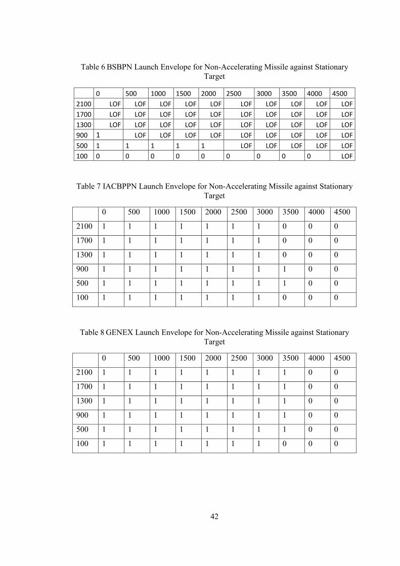
42
Table 6 BSBPN Launch Envelope for Non-Accelerating Missile against Stationary Target
0 500 1000 1500 2000 2500 3000 3500 4000 4500
2100 LOF LOF LOF LOF LOF LOF LOF LOF LOF LOF
1700 LOF LOF LOF LOF LOF LOF LOF LOF LOF LOF
1300 LOF LOF LOF LOF LOF LOF LOF LOF LOF LOF
900 1 LOF LOF LOF LOF LOF LOF LOF LOF LOF
500 1 1 1 1 1 LOF LOF LOF LOF LOF
100 0 0 0 0 0 0 0 0 0 LOF
Table 7 IACBPPN Launch Envelope for Non-Accelerating Missile against Stationary Target
0 500 1000 1500 2000 2500 3000 3500 4000 4500
2100 1 1 1 1 1 1 1 0 0 0
1700 1 1 1 1 1 1 1 0 0 0
1300 1 1 1 1 1 1 1 0 0 0
900 1 1 1 1 1 1 1 1 0 0
500 1 1 1 1 1 1 1 1 0 0
100 1 1 1 1 1 1 1 0 0 0
Table 8 GENEX Launch Envelope for Non-Accelerating Missile against Stationary Target
0 500 1000 1500 2000 2500 3000 3500 4000 4500
2100 1 1 1 1 1 1 1 1 0 0
1700 1 1 1 1 1 1 1 1 0 0
1300 1 1 1 1 1 1 1 1 0 0
900 1 1 1 1 1 1 1 1 0 0
500 1 1 1 1 1 1 1 1 0 0
100 1 1 1 1 1 1 1 0 0 0

43
Table 9 SDREGL Launch Envelope for Non-Accelerating Missile against Stationary Target
0 500 1000 1500 2000 2500 3000 3500 4000 4500
2100 1 1 1 1 1 1 1 0 0 0
1700 1 1 1 1 1 1 1 0 0 0
1300 1 1 1 1 1 1 1 1 0 0
900 1 1 1 1 1 1 1 1 0 0
500 1 1 1 1 1 1 1 1 0 0
100 1 1 1 1 1 1 1 0 0 0
Table 10 OG Launch Envelope for Non-Accelerating Missile against Stationary Target
0 500 1000 1500 2000 2500 3000 3500 4000 4500
2100 1 1 1 1 1 0 0 0 0 0
1700 1 1 1 1 1 1 0 0 0 0
1300 1 1 1 1 1 1 1 0 0 0
900 1 1 1 1 1 1 1 0 0 0
500 1 1 1 1 1 1 1 1 0 0
100 1 1 1 1 1 0 0 0 0 0
4.1.2.2 Miss Distance Contours
In this sub-section, launch envelope is analyzed from a different perspective. Miss
distance values in the defined field are calculated using a more refined mesh.
Contours will not be shown for BSBPN since lock-on-failure happens for most of the
field.
Table 11 Simulation Properties
Parameters Values
Missile Initial Position Varies in the defined field
Missile Initial Position
Sampling Interval
100 meters for downrange
80 meters for altitude
Target Initial Position (5000,0)

44
Target Velocity Stationary
Missile Velocity 250 m/sec
Missile Initial Orientation +15 degrees
Gravity Neglected
Desired Impact Angle -45 degrees
Acceleration Limits +7g/-7g
Figure 14 Miss Distance Contours for IACBPPN (Stationary)
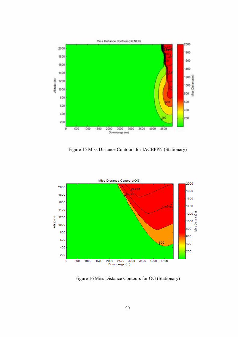
45
Figure 15 Miss Distance Contours for IACBPPN (Stationary)
Figure 16 Miss Distance Contours for OG (Stationary)

46
Figure 17 Miss Distance Contours for SDREGL (Stationary)
4.1.2.3 Cost Function Contours
Investigating only the miss distance might be misleading. Hence, a cost function is
defined which would help to judge the picture in another sense. Cost function is
defined as:
½wS� ¾�<��Rw< = �RSS ¿RS��<�]�<R�R�} ¿RS��<�] (85)

47
Figure 18 Cost Function Contours for IACBPPN (stationary)
Figure 19 Cost Function Contours for GENEX (stationary)

48
Figure 20 Cost Function Contours for OG (stationary)
Figure 21 Cost Function Contours for SDREGL (stationary)
It is not surprising that OG has the worst cost function characteristic of above all
since its miss distance contours also showed poor performance. GENEX and

49
SDREGL show similar characteristic. IACBPPN can be concluded to be having a
moderate performance.
4.1.3 Run Type III
TGH orientation varies depending on the scenario defined. For this reason, analyses
carried out to see the impact of variation of TGH orientation to the impact angle and
miss distance. Recalling the missile envelope extraction (see section 4.1.2) for initial
orientation of +15 degrees, not all points in launch envelope will be analyzed. Only 4
points which might be considered as critical are analyzed and these points vary
depending on the law due to fact that their successful and unsuccessful launch points
are different. For each law, the points that are considered to be critical and tested for
robustness against initial TGH angle are presented in Table 11.
Table 12 TGH Angle Test Points
Law
Point # BSBPN IACBPPN GENEX SDREGL OG
Point I (0,100) (3000,900) (3500,900) (3500,900) (3500,500)
Point II (0,500) (3000,1300) (3500,1300) (3500,1300) (3500,900)
Point III (500,100) (3500,900) (4000,900) (4000,900) (4000,500)
Point IV (500,500) (3500,1300) (4000,1300) (4000,1300) (4000,900)
TGH angles are changed as below:
��� = −10, −5,0,5,10,15 (86)
For all laws, point I trajectories will be visualized whereas other points’ only results
will be given for sake of brevity.
4.1.3.1 BSBPN Success Investigation
Trajectories for the five TGH angles shown in (86) for the TGH point I are plotted in
Figure 22. Numerical assessment of these trajectories together with the results of
other TGH angle test points is tabulated in Table 13.

50
Figure 22 Missile Trajectory for Different TGH Orientation
Table 13 Success Chart of BSBPN for Various TGH Orientation
-10 -5 0 5 10 15
(0,100) 1 1 1 1 0 0
(0,500) 1 1 1 1 1 1
(500,100) 1 1 1 0 0 0
(500,500) 1 1 1 1 1 1
4.1.3.2 IACBPPN Success Investigation
For point I, the figure below illustrates the trajectory of missiles subjected to
different initial TGH angles for IACBPPN.
0 500 1000 1500 2000 2500 3000 3500 4000 4500 50000
100
200
300
400
500
600
700
800
900Missile Trajectory(BSBPN)
Downrange(m)
Altitude(m
)

51
Figure 23 Missile Trajectory History for Various TGH Orientation (IACBPPN)
Table 14 Success Chart of IACBPPN for Various TGH Orientation
-10 -5 0 5 10 15
(3000,900) 1 1 1 1 1 1
(3000,1300) 1 1 1 1 1 1
(3500,900) 1 1 1 1 1 1
(3500,1300) 1 1 1 1 0 0
3000 3200 3400 3600 3800 4000 4200 4400 4600 4800 50000
100
200
300
400
500
600
700
800
900
1000Missile Trajectory(IACBPPN)
Downrange(m)
Altitude(m
)

52
4.1.3.3 GENEX Success Investigation
For point I, the figure below illustrates the trajectory of missiles subjected to
different TGH angles for GENEX. The figure shows that when the missile switches
to the terminal guidance at point I, the missile successfully intercepts the target at the
commanded angle for all TGH angles tested. Results for all test points are tabulated
in Table 15.
Figure 24 Missile Trajectory History for Various TGH Orientation (GENEX)
Table 15 Success Chart of GENEX for Various TGH Angles
-10 -5 0 5 10 15
(3500,900) 1 1 1 1 1 1
(3500,1300) 1 1 1 1 1 1
(4000,900) 1 1 0 0 0 0
(4000,1300) 1 0 0 0 0 0
3500 4000 4500 50000
100
200
300
400
500
600
700
800
900
1000Missile Trajectory(GENEX)
Downrange(m)
Altitude(m
)

53
4.1.3.4 SDREGL Success Investigation
For point I, the figure below illustrates the trajectory of missiles subjected to
different TGH angles for SDREGL. Similar to the previous cases, all five TGH
angles lead to successful intercept. Test points III and IV should be considered
outside the allowable launch zone since the missile fails for almost all TGH angles
tested as seen in Table 16.
Figure 25 Missile Trajectories for Various TGH Angles (SDREGL)
3500 4000 4500 50000
100
200
300
400
500
600
700
800
900
1000Missile Trajectory(SDREGL)
Downrange(m)
Altitude(m
)

54
Table 16 Success Chart of SDREGL for Various TGH Angles
-10 -5 0 5 10 15
(3500,900) 1 1 1 1 1 1
(3500,1300) 1 1 1 1 1 1
(4000,900) 1 0 0 0 0 0
(4000,1300) 0 0 0 0 0 0
4.1.3.5 OG Success Investigation
For point I, the figure below illustrates the trajectory of missiles subjected to
different TGH angles for OG. . The figure shows that for point I TGH angle is
critical and should be chosen to be positive as for the negative angles tested the
missile fails to satisfy performance requirements. Results for all test points are
presented in Table 17.
Figure 26 Missile Trajectories for Various TGH Angles (OG)
3400 3600 3800 4000 4200 4400 4600 4800 5000 52000
100
200
300
400
500
600
700Missile Trajectory(OG)
Downrange(m)
Altitude(m
)

55
Table 17 Success Chart of OG for Various TGH Angles
-10 -5 0 5 10 15
(3500,500) 0 0 1 1 1 1
(3500,900) 1 1 1 1 1 0
(4000,500) 1 1 1 0 0 0
(4000,900) 0 0 0 0 0 0
4.1.3.6 Comments on Run Type III
As seen in all tables in this sub-section, success varies upon the TGH angle. This
results show that, in practice, it would be important to carefully approach the target
so that at the TGH point, the missile orientation is appropriate for a successful strike.
Results obtained by run types II and III can be used to increase the success rate of a
missile. The missile should be taken by the midcourse guidance algorithm to a safe
point in the allowable launch zone before switching to terminal guidance such that
even moderate errors in reaching the desired TGH point should not jeopardize the
mission. While selecting the TGH point, sensitivity to TGH angle should also be
taken into account in order to maximize the chances of success.
4.2 Non-Stationary Target
In this subsection, investigated algorithms will be analyzed in the case of a non-
stationary non-maneuvering target.
4.2.1 Run Type I
GENEX and OG are the laws that take the target motion into account. Hence,
satisfactory performance is expected from those algorithms. The other algorithms are
for stationary targets; however they will also be analyzed in this section to illustrate
the reader that these algorithms cannot satisfy either or both of the performance
criterions in case of non-stationary targets.
The algorithm parameters are the same as used in section 4.1.1. The engagement
parameters are the same expect that in this case there is a target motion which is 15

56
m/sec symbolizing a main battle tank target. The parameters are given in Table 18.
Trajectories with all five guidance laws for this sample scenario are presented in
Figure 27.
Table 18 Scenario II Run I Parameters
The target is intercepted by all guidance laws, however the impact angle error is
within acceptable limits for only GENEX and OG as expected. This can clearly be
seen in Figure 28. While both of these laws satisfy the performance requirements,
they have considerably different acceleration profiles as seen in Figure 29. The OG
starts off with a very little acceleration command and at around � = 3 seconds it
suddenly commands a very large acceleration reaching the acceleration limit due to
the fact that guidance phases are switched. After about 1.5 seconds it comes out of
saturation and reaches the target with a decaying acceleration command. GENEX
algorithm on the other hand never reaches acceleration limit up until the intercept
point. Numerical comparison of all five performances is presented in Table 19.
Parameters Values
Missile Initial Position (3000,500)
Target Initial Position (5000,0)
Target Velocity 15 m/sec
Missile Initial Velocity 250 m/sec
Missile Initial Orientation +15 degrees
Gravity Neglected
Desired Impact Angle -45 degrees
Acceleration Limits +7g/-7g

57
Figure 27 Missile Trajectory Histories
Figure 28 Flight Path Angle Histories
3000 3500 4000 4500 5000 5500-100
0
100
200
300
400
500
600
700
800Missile Trajectory
Downrange(m)
Altitude(m)
BSBPN
IACBPPN
GENEX
SDREGL
OG
0 1 2 3 4 5 6 7 8 9 10-50
-40
-30
-20
-10
0
10
20Flight Path Angle
Time(s)
Angle(degrees)
BSBPN
IACBPPN
GENEX
SDREGL
OG

58
Figure 29 Acceleration Histories
Table 19 Scenario II Run I Results
BSBPN IACBPPN GENEX SDREGL OG
Miss
Distance(m)
1.97 1.51 3.27 2.29 0.72
Impact
Angle(degrees)
-33.1 -32.5 -45.0 -40.56 -45.0
Control
Effort(m/s)
311.9 251.56 263.4 254.8 261.9
BSBPN, IACBPPN and SDREGL are not expected to satisfy the desired criterions.
The results met this expectation since they are not designed to intercept non-
stationary targets. GENEX and OG as expected perfectly satisfy success criterions.
0 1 2 3 4 5 6 7 8 9 10-80
-60
-40
-20
0
20
40
60
80Acceleration History
Time(s)
Acceleration(m
/s2)
BSBPN
IACBPPN
GENEX
SDREGL
OG

59
Moreover, it should be noted that BSBPN needs more control effort to intercept the
target than that others do.
4.2.1.1 Simulation with Gravity ON for Non-Stationary Target
Simulation parameters are seen below in Table 20.
Table 20 Simulation Parameters for Non-Stationary Targets with Gravity
Parameters Values
Missile Initial Position (3000,500)
Target Initial Position (5000,0)
Missile Initial Velocity 250 m/s
Missile Initial Orientation +15 degrees
Target Velocity 15 m/sec
Target Orientation +x direction
Gravity Neglected
Desired Impact Angle -45 degrees
Acceleration Limits +7g/-7g
Gravity ON
Table 21 Results with Gravity for Non-Stationary Target
BSBPN IACBPPN GENEX SDREGL OG
Miss
Distance(m)
2.4 1.0 4.0 0.1 2.4
Impact
Angle(degrees)
-34.0 -33.9 -44.9 -40.8 -45.0
Control
Effort(m/s)
306.7 244.2 264.3 276.2 257.6

60
One should compare Table 19 and Table 21 to see the effects of gravity. The results
are the same with the stationary target case. Almost no difference exists for this
scenario between gravity on and gravity off cases. This shows that gravity
compensation can successfully remove the effect of gravity even though the
component of gravity along the body ¦ axis cannot be compensated for.
4.2.2 Run Type II
4.2.2.1 Discrete TGH Region
In this section, the same procedure that was applied in section 4.1.2 will be processed
but for this time the target is non-stationary whose velocity is 15 m/sec in +x
direction. The aim is again to extract the allowable missile launch regions in terms of
successful intercept with the desired impact angle. Parameters of the run are below.
Table 22 Scenario II Run II Parameters
Since the only law designed for non-stationary targets is GENEX, only launch
envelope extracted is GENEX for non-stationary targets case.
Parameters Values
Missile Initial Position Varies in the defined field
Target Initial Position (5000,0)
Target Velocity 15 m/sec
Target Orientation +x direction
Missile Initial Velocity 250 m/sec
Missile Initial Orientation +15 degrees
Gravity Neglected
Desired Impact Angle -45 degrees
Acceleration Limits +7g/-7g
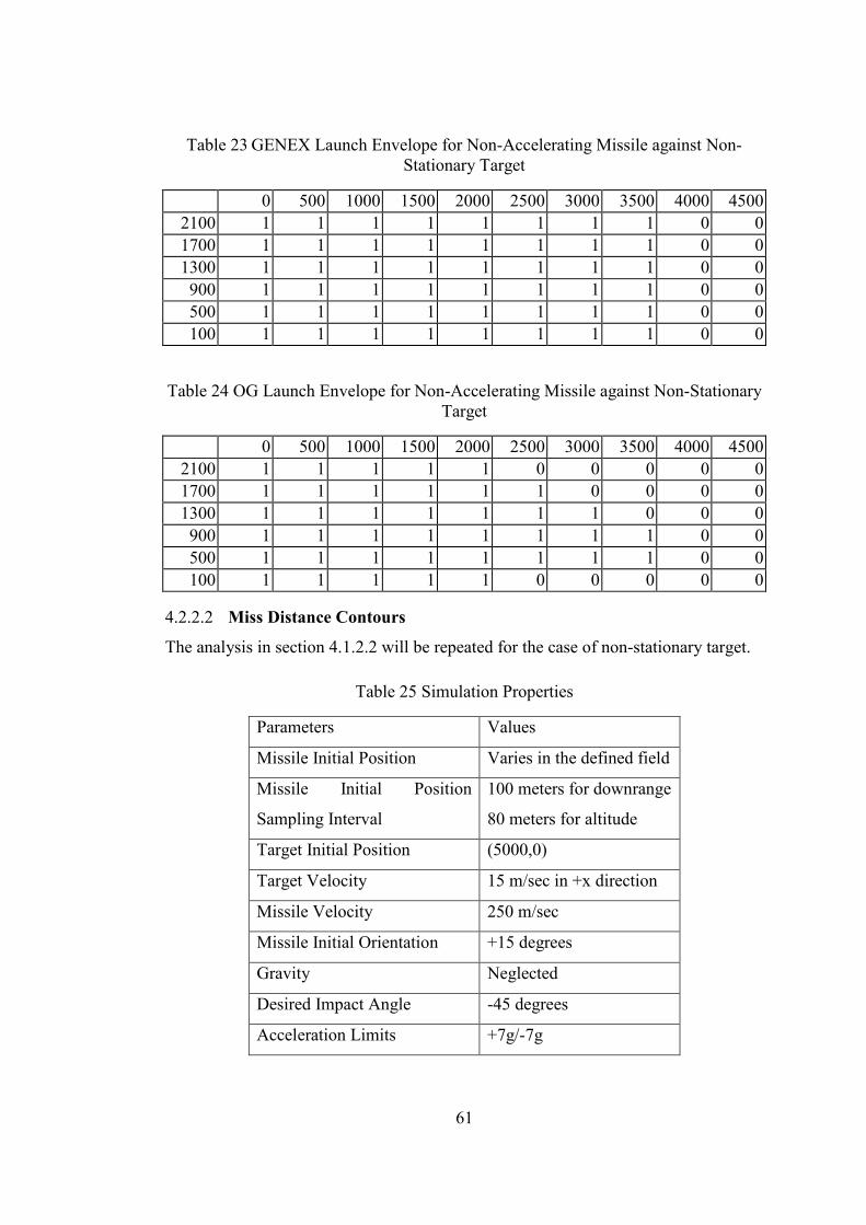
61
Table 23 GENEX Launch Envelope for Non-Accelerating Missile against Non-Stationary Target
0 500 1000 1500 2000 2500 3000 3500 4000 4500 2100 1 1 1 1 1 1 1 1 0 0 1700 1 1 1 1 1 1 1 1 0 0 1300 1 1 1 1 1 1 1 1 0 0 900 1 1 1 1 1 1 1 1 0 0 500 1 1 1 1 1 1 1 1 0 0 100 1 1 1 1 1 1 1 1 0 0
Table 24 OG Launch Envelope for Non-Accelerating Missile against Non-Stationary Target
0 500 1000 1500 2000 2500 3000 3500 4000 4500 2100 1 1 1 1 1 0 0 0 0 0 1700 1 1 1 1 1 1 0 0 0 0 1300 1 1 1 1 1 1 1 0 0 0 900 1 1 1 1 1 1 1 1 0 0 500 1 1 1 1 1 1 1 1 0 0 100 1 1 1 1 1 0 0 0 0 0
4.2.2.2 Miss Distance Contours
The analysis in section 4.1.2.2 will be repeated for the case of non-stationary target.
Table 25 Simulation Properties
Parameters Values
Missile Initial Position Varies in the defined field
Missile Initial Position
Sampling Interval
100 meters for downrange
80 meters for altitude
Target Initial Position (5000,0)
Target Velocity 15 m/sec in +x direction
Missile Velocity 250 m/sec
Missile Initial Orientation +15 degrees
Gravity Neglected
Desired Impact Angle -45 degrees
Acceleration Limits +7g/-7g

62
Figure 30 Miss Distance Contours for GENEX (non-stationary)
Figure 31 Miss Distance Contours for OG (non-stationary)

63
4.2.2.3 Cost Function Contours
Figure 32 Cost Function Contours for GENEX (non-stationary)
Figure 33 Cost Function Contours for OG (non-stationary)

64
4.2.3 Run Type III
This is the same run type in section 4.1.2.2. However, in this section, target will be
non-stationary with the orientation and velocity being +x and +15 m/sec respectively.
The TGH coordinates are seen in the table below.
Table 26 TGH Test Points
Law
Point # GENEX OG
Point I (3500,500) (3500,900)
Point II (3500,900) (3500,1300)
Point III (4000,500) (4000,900)
Point IV (4000,900) (4000,1300)
For all laws, point I trajectories will be visualized only.

65
4.2.3.1 GENEX Success Investigation
Figure 34 Missile Trajectory for Various TGH Angles
Table 27 Success Chart of GENEX for TGH Angles (non-stationary target)
-10 -5 0 5 10 15
(3500,500) 1 1 1 1 1 1
(3500,900) 1 1 1 1 1 1
(4000,500) 1 1 1 1 1 0
(4000,900) 1 1 1 0 0 0
4.2.3.2 OG Success Investigation
3400 3600 3800 4000 4200 4400 4600 4800 5000 5200-100
0
100
200
300
400
500
600Missile Trajectory(GENEX)
Downrange(m)
Altitude(m)

66
Figure 35 Missile Trajectory for TGH Angles
Table 28 Success Chart of GENEX for Various TGH Angles (non-stationary target)
-10 -5 0 5 10 15
(3500,900) 1 1 1 1 1 1
(3500,1300) 1 1 0 0 0 0
(4000,900) 0 0 0 0 0 0
(4000,1300) 0 0 0 0 0 0
4.2.3.3 Comments on Run Type III
Results are similar with the results explained in section 4.1.3.6. Recalling that, in
order to ensure a satisfactory performance, missile firing officer and/or pilot should
be careful when directing the missile to the target.
3400 3600 3800 4000 4200 4400 4600 4800 5000 52000
100
200
300
400
500
600
700
800
900
1000Missile Trajectory(OG)
Downrange(m)
Altitude(m
)

67
4.2.4 Run Type IV
In this section, target velocity will be varied between -30 and +30 m/sec and the
success of algorithms will be investigated.
It would be good to discriminate 5 algorithms that are investigated in detail to 2 parts
in this test. In the first part, the algorithms that are designed for stationary targets will
be tested whereas in the second part the algorithms that are designed for non-
stationary targets will be tested against non-stationary targets.
Output will be scatter graphs in which the intercept angles and miss distances exist.
Below, there exist the parameters of the run.
Table 29 Scenario II Run IV Parameters
Parameters Values
Missile Initial Position (3000,500)
Target Initial Position (5000,0)
Target Velocity Varies between -30 to
+30 m/sec with 5 m/sec
intervals
Missile Initial Velocity 250 m/sec
Missile Initial Orientation +15 degrees
Gravity Neglected
Desired Impact Angle -45 degrees
Acceleration Limits +7g/-7g

68
4.2.4.1 Run Type IV for Stationary Type Algorithms
Figure 36 Scatter Graph for BSBPN
Figure 37 Scatter Graph for IACBPPN
0
2
4
6
8
10
12
-75 -70 -65 -60 -55 -50 -45 -40 -35 -30 -25 -20 -15 -10 -5 0
-30 m/s
-25m/s
-20 m/s
-15 m/s
-10 m/s
- 5 m/s
0 m/s
5 m/s
10 m/s
15m/s
20 m/s
25 m/s
30 m/s
0
5
10
15
20
25
-75 -70 -65 -60 -55 -50 -45 -40 -35 -30 -25 -20 -15 -10 -5 0
-30 m/s
-25 m/s
-20 m/s
-15 m/s
-10 m/s
-5 m/s
0 m/s
5 m/s
10 m/s
15 m/s
20 m/s
25 m/s
30 m/s

69
Figure 38 Scatter Graph for SDREGL
In Figure 36, Figure 37 and Figure 38, it is observed that for different target
velocities, miss distances and impact angles vary. A “good” algorithm should not
have a very big variance of miss distance and impact angle for different target
speeds. In this manner, the best algorithm of above algorithms is SDREGL.
0
0,5
1
1,5
2
2,5
-75 -70 -65 -60 -55 -50 -45 -40 -35 -30 -25 -20 -15 -10 -5 0
-30 m/s
-25 m/s
-20 m/s
-15 m/s
-10 m/s
-5 m/s
0 m/s
5 m/s
10 m/s
15 m/s
20 m/s
25 m/s
30 m/s
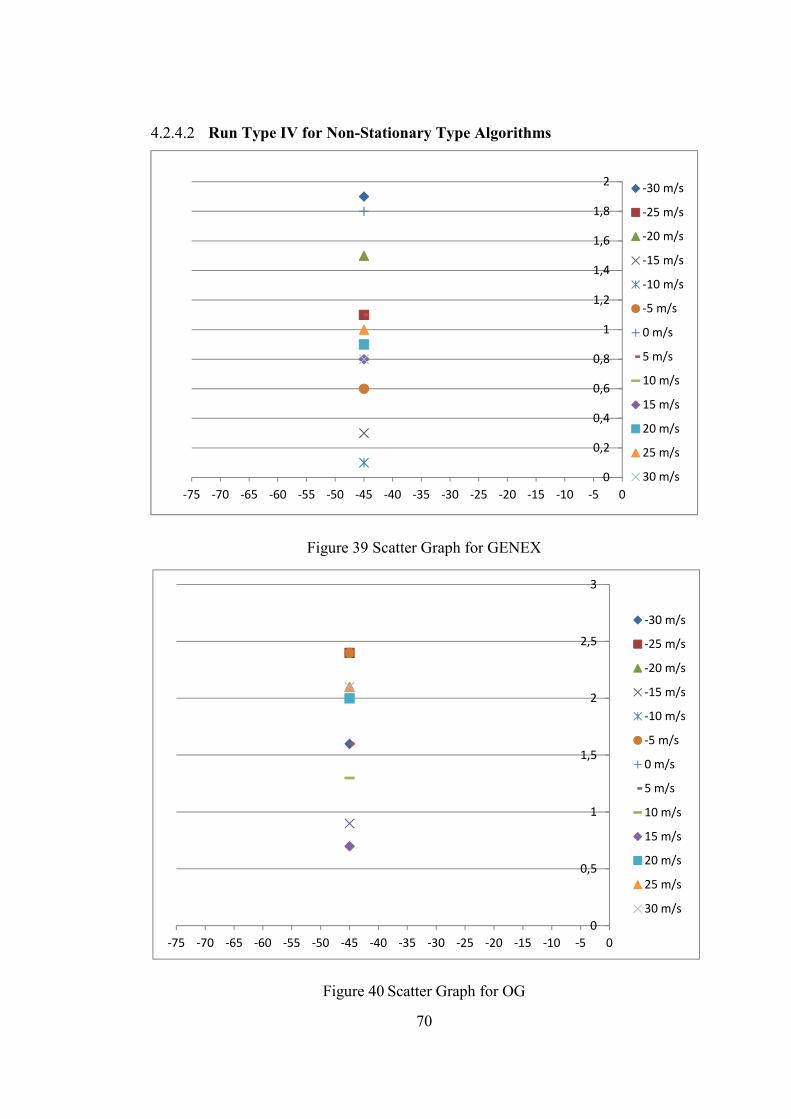
70
4.2.4.2 Run Type IV for Non-Stationary Type Algorithms
Figure 39 Scatter Graph for GENEX
Figure 40 Scatter Graph for OG
0
0,2
0,4
0,6
0,8
1
1,2
1,4
1,6
1,8
2
-75 -70 -65 -60 -55 -50 -45 -40 -35 -30 -25 -20 -15 -10 -5 0
-30 m/s
-25 m/s
-20 m/s
-15 m/s
-10 m/s
-5 m/s
0 m/s
5 m/s
10 m/s
15 m/s
20 m/s
25 m/s
30 m/s
0
0,5
1
1,5
2
2,5
3
-75 -70 -65 -60 -55 -50 -45 -40 -35 -30 -25 -20 -15 -10 -5 0
-30 m/s
-25 m/s
-20 m/s
-15 m/s
-10 m/s
-5 m/s
0 m/s
5 m/s
10 m/s
15 m/s
20 m/s
25 m/s
30 m/s

71
For both GENEX and OG, not much variance is observed and they can be considered
as successful for the target speeds defined.
4.3 Robustness to Time Constant
In all analyses above, time constant of the missile was taken to be 0.25 seconds.
However, it may depend from the missile to missile in real applications. In this
section, all of the 5 laws will be tested against various time constant values and
success of them in terms of miss distance and impact angle is analyzed.
4.3.1 Robustness to Time Constant Against Stationary Target
All 5 laws will be analyzed against stationary target with the time constants being in
the range between 0 and 1. Simulation parameters are the same as those shown in
Table 1.
Figure 41 Miss Distance vs. Time Constant (stationary target)
0 0.1 0.2 0.3 0.4 0.5 0.6 0.7 0.8 0.9 10
5
10
15
20
25Miss Distance vs. Time Constant
Time Constant(s)
Miss Distance(m
)
BSBPN
IACBPPN
GENEX
SDREGL
OG

72
Figure 42 Impact Angle Error vs. Time Constant (stationary target)
In Figure 41, it is observed that miss distances of all laws are in acceptable range in
the specified time constant interval. The jumpiness of the curves in Figure 41 is
caused by the way miss distance is calculated. To reduce simulation run times,
integration time step is chosen as 0.01 seconds as explained in the beginning of
section 4. At a speed of 250 m/s, the missile travels about 2.5 meters in one time
step. Hence the accuracy of miss distance calculation is less than 2.5 meters. Hence
the results in Figure 41 in fact demonstrate perfect hit within the accuracy of miss
distance calculations.
In Figure 42, it is seen that GENEX, SDREGL and OG are more robust than the
other two laws in terms of impact angle error. They virtually have no impact angle
error in the specified time constant interval. On the contrary, IACBPPN has an
increasing trend of impact angle error. This would badly affect the performance of
the missile when the time constant gets larger. On the other hand, BSBPN has a
stable impact angle error characteristic which might be an advantage in the case of an
unknown system, i.e. a missile in conceptual design phase.
0 0.2 0.4 0.6 0.8 1 1.2 1.40
0.5
1
1.5
2
2.5
3
3.5Impact Angle Error vs.Time Constant
Time Constant(s)
Impact Angle Error(degrees)
BSBPN
IACBPPN
GENEX
SDREGL
OG

73
4.3.2 Robustness to Time Constant Against Non-Stationary Targets
In this subsection, contrary to previous section, simulations are run for non-stationary
targets for 2 laws that are designed for non-stationary targets. Simulation parameters
are the same as Table 18.
Figure 43 Miss Distance vs. Time Constant (non-stationary target)
0 0.2 0.4 0.6 0.8 1 1.2 1.40
0.5
1
1.5
2
2.5
3
3.5
4
4.5
5Miss Distance vs. Time Constant
Time Constant(s)
Miss Distance(m)
GENEX
OG

74
Figure 44 Impact Angle vs. Time Constant (non-stationary target)
In Figure 43 and in Figure 44, it is seen that impact angle and miss distance
performance of both GENEX and OG are not distorted by the time constants up to 1
seconds.
4.4 Time-to-Go Error Analysis
Time to go information is needed in GENEX and SDREGL. Hence, it would be
good to analyze the effect of time-to-go error. The error model is taken from [11] and
is simply stated as following:
�¹�² = À��² + ∆��² (87)
Effects of proportional and additive terms will be analyzed separately. One important
note is that the impact angle error is only meaningful where the impact really
happens. Otherwise, it is nothing but the flight path angle at the location where it is
closest to the target. Hence, the portion of the impact angle error graphs where the
miss distance is less than 20 m. will be zoomed so that conclusions can be drawn
more easily. If there are two laws being compared, depending on the miss distance
history, all portion of impact angle error graph may be visualized since the miss
0 0.2 0.4 0.6 0.8 1 1.2 1.40
0.02
0.04
0.06
0.08
0.1
0.12
0.14
0.16Impact Angle Error vs.Time Constant
Time Constant(s)
Impact Angle Error(degrees)
GENEX
OG
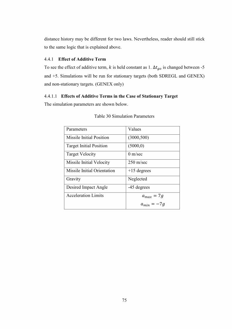
75
distance history may be different for two laws. Nevertheless, reader should still stick
to the same logic that is explained above.
4.4.1 Effect of Additive Term
To see the effect of additive term, À is held constant as 1. ∆��² is changed between -5
and +5. Simulations will be run for stationary targets (both SDREGL and GENEX)
and non-stationary targets. (GENEX only)
4.4.1.1 Effects of Additive Terms in the Case of Stationary Target
The simulation parameters are shown below.
Table 30 Simulation Parameters
Parameters Values
Missile Initial Position (3000,500)
Target Initial Position (5000,0)
Target Velocity 0 m/sec
Missile Initial Velocity 250 m/sec
Missile Initial Orientation +15 degrees
Gravity Neglected
Desired Impact Angle -45 degrees
Acceleration Limits ��_` = 7� ��U� = −7�

76
Figure 45 Miss Distance Error due to Time to go Error (additive/ stationary target)
Figure 46 Impact Angle Error due to Time to go Error (additive/ stationary target)
-5 -4 -3 -2 -1 0 1 2 3 4 50
20
40
60
80
100
120
140
160Miss Distance Error due to Time to go Error
Additive Term(s)
Miss Distance Error(m)
GENEX
SDREGL
-2 -1 0 1 2 3 4 5
0
2
4
6
8
10
12
14
Impact Angle Error due to Time to go Error
Additive Term(s)
Impact Angle Error(degrees)
GENEX
SDREGL

77
In the case explained above, it is observed that additive term has a distorting effect
when it is negative which means time-to-go is under-estimated. On the contrary,
when it is positive, it doesn’t have a much disturbance which means time-to-go is
over-estimated. The advantage of one law over the other is highly dependent on the
specific error interval. The sharp jumps occurring in the additive term type graphs
are due to acceleration saturation difference between the corresponding error terms.
4.4.1.2 Effects of Additive Terms in the Case of Non-Stationary Target
SDREGL is not designed for non-stationary targets. Hence it would not make any
sense to evaluate its performance in this analysis. Only GENEX will be analyzed in
this subsection.
The simulation parameters are shown below.
Table 31 Simulation Parameters
Parameters Values
Missile Initial Position (3000,500)
Target Initial Position (5000,0)
Missile Initial Velocity 250 m/sec
Missile Initial Orientation +15 degrees
Target Orientation +x direction
Target Velocity 15 m/sec
Gravity Neglected
Desired Impact Angle -45 degrees
Acceleration Limits ��_` = 7� ��U� = −7�

78
Figure 47 Miss Distance Error due to Time to go Error (additive/non-stationary target)
Figure 48 Impact Angle Error due to Time to go Error (additive/ non-stationary target)
-5 -4 -3 -2 -1 0 1 2 3 4 50
20
40
60
80
100
120Miss Distance Error due to Time to go Error(additive)
Additive Term(s)
Miss Distance Error(m)
GENEX
-2 -1 0 1 2 3 4 50
2
4
6
8
10
12
14
16
Impact Angle Error due to Time to go Error(additive)
Additive Term(s)
Impact Angle Error(degrees)
GENEX

79
GENEX has almost same trend with the stationary type case. One can comment with
confidence that over-estimation is advantageous than under-estimation. The sharp
jumps occurring in the additive term type graphs are due to acceleration saturation
difference between the corresponding error terms.
4.4.2 Effect of Proportional Term
To see the effect of proportional term, ∆��² is set to 0 whereas À is changed between
0.4 and 2. Simulations will be run for stationary targets (both SDREGL and GENEX)
and non-stationary targets. (GENEX only)
4.4.2.1 Effects of Proportional Term in the Case of Stationary Target
Simulation parameters are the same as Table 30.
Figure 49 Miss Distance Error due to Time to go Error (proportional/stationary)
0.4 0.6 0.8 1 1.2 1.4 1.6 1.8 2 2.2 2.40
10
20
30
40
50
60
70
80Miss Distance Error due to Time to go Error(proportional)
Proportional Term(unitless)
Miss Distance Error(m)
GENEX
SDREGL

80
Figure 50 Impact Angle Error due to Time to go Error (proportional/stationary)
It is worth to note that for proportional term between 0.6 and 2 (for GENEX, whole
range between 0.4 and 2) both laws show superior performance. It means under-
estimation of 40% and over-estimation of 100% does not affect the performance.
4.4.2.2 Effects of Proportional Terms in the Case of Non-Stationary Target
Simulation parameters are the same as Table 31.
0.4 0.6 0.8 1 1.2 1.4 1.6 1.8 2 2.2 2.40
2
4
6
8
10
12
14
16
18
20Impact Angle Error due to Time to go Error(proportional)
Proportional Term(unitless)
Impact Angle Error(degrees)
GENEX
SDREGL

81
Figure 51 Miss Distance Error due to Time to go Error (proportional/non-stationary)
Figure 52 Impact Angle Error due to Time to go Error (proportional /non-stationary)
0.4 0.6 0.8 1 1.2 1.4 1.6 1.8 2 2.2 2.40
0.2
0.4
0.6
0.8
1
1.2
1.4Miss Distance Error due to Time to go Error(proportional)
Proportional Term(unitless)
Miss Distance Error(m)
GENEX
0.4 0.6 0.8 1 1.2 1.4 1.6 1.8 2 2.2 2.40
0.05
0.1
0.15
0.2
0.25
0.3
0.35Impact Angle Error due to Time to go Error(proportional)
Proportional Term(unitless)
Impact Angle Error(degrees)
GENEX

82
GENEX shows good performance in the case of non-stationary target also.
4.5 Time-to-go Error Analysis with Non-Traditional Time-to-Go
Method[1]
In both of the two algorithms that require time-to-go information, time-to-go is
calculated by the traditional formulation which is nothing but range divided by
missile velocity. However, as seen in [1], there are other methods that can be used to
calculate time-to-go which might improve the guidance performance. This section is
devoted to the time-to-go error analysis’ with traditional and new time-to-go method
described in [1].
There are two time-to-go calculation methods in [1] both of which will be explained
in the appendix section. In simulations, method 2 shall be used for the reasons that
are explained in the appendix.
4.5.1 Additive Term Varying Case
4.5.1.1 GENEX Time-to-go Error Analysis Comparison with New Time-to-go
Method Against Non-Stationary Target
The simulation parameters are shown below.
Table 32 Simulation Parameters
Parameters Values
Missile Initial Position (3000,500)
Target Initial Position (5000,0)
Missile Initial Velocity 250 m/sec
Missile Initial Orientation +15 degrees
Target Orientation +x direction

83
Target Velocity 15 m/sec
Gravity Neglected
Desired Impact Angle -45 degrees
Acceleration Limits ��_` = 7� ��U� = −7�

84
Figure 53 Miss Distance Error due to Time to go Error (additive/non-stationary)
Figure 54 Impact Angle Error due to Time to go Error (additive/non-stationary)
-5 -4 -3 -2 -1 0 1 2 3 4 50
50
100
150
200
250
300
350
400
450
500Miss Distance Error due to Time to go Error(additive)
Additive Term(s)
Miss Distance Error(m)
GENEX Traditional
GENEX Tgo New
-2 -1 0 1 2 3 4 5
0
2
4
6
8
10
12
14
16
18
20
Impact Angle Error due to Time to go Error(additive)
Additive Term(s)
Impact Angle Error(degrees)
GENEX Traditional
GENEX Tgo New

85
As seen in the figures above, for terms from -2 to 5 seconds both method show
similar performance. From -5 to -2, traditional method shows better performance
though both cannot satisfy success criterions in that interval.
4.5.1.2 SDREGL Time-to-go Error Analysis Comparison with New Time-to-go
Method against Stationary Target
Simulation parameters are shown below.
Parameters Values
Missile Initial Position (3000,500)
Target Initial Position (5000,0)
Target Velocity 0 m/sec
Missile Initial Velocity 250 m/sec
Missile Initial Orientation +15 degrees
Gravity Neglected
Desired Impact Angle -45 degrees
Acceleration Limits ��_` = 7� ��U� = −7�

86
Figure 55 Miss Distance Error due to Time to go Error (additive/stationary)
Figure 56 Impact Angle Error due to Time to go Error (additive/stationary)
-5 -4 -3 -2 -1 0 1 2 3 4 50
20
40
60
80
100
120
140
160Miss Distance Error due to Time to go Error
Additive Term(s)
Miss Distance Error(m)
SDREGL Traditional
SDREGL Tgo New
-1 0 1 2 3 4 5
0
1
2
3
4
5
6
7
8
9
10
Impact Angle Error due to Time to go Error
Additive Term(s)
Impact Angle Error(degrees)
SDREGL Traditional
SDREGL Tgo New
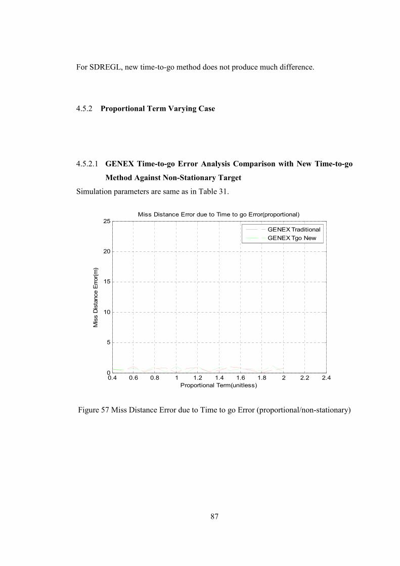
87
For SDREGL, new time-to-go method does not produce much difference.
4.5.2 Proportional Term Varying Case
4.5.2.1 GENEX Time-to-go Error Analysis Comparison with New Time-to-go
Method Against Non-Stationary Target
Simulation parameters are same as in Table 31.
Figure 57 Miss Distance Error due to Time to go Error (proportional/non-stationary)
0.4 0.6 0.8 1 1.2 1.4 1.6 1.8 2 2.2 2.40
5
10
15
20
25Miss Distance Error due to Time to go Error(proportional)
Proportional Term(unitless)
Miss Distance Error(m)
GENEX Traditional
GENEX Tgo New

88
Figure 58 Impact Angle Error due to Time to go Error (proportional/non-stationary)
GENEX law with new time-to-go method also shows superior performance in the
existence of proportional error term.
4.5.2.2 SDREGL Time-to-go Error Analysis Comparison with New Time-to-go
Method Against Stationary Target
Simulation parameters are same as in Table 32.
0.4 0.6 0.8 1 1.2 1.4 1.6 1.8 2 2.2 2.40
0.5
1
1.5
2
2.5
3
3.5
4
4.5
5Impact Angle Error due to Time to go Error(proportional)
Proportional Term(unitless)
Impact Angle Error(degrees)
GENEX Traditional
GENEX Tgo New

89
Figure 59 Miss Distance Error due to Time to go Error (proportional/ stationary)
Figure 60 Impact Angle Error due to Time to go Error (proportional/ stationary)
0.4 0.6 0.8 1 1.2 1.4 1.6 1.8 2 2.2 2.40
10
20
30
40
50
60
70
80Miss Distance Error due to Time to go Error(proportional)
Proportional Term(unitless)
Miss Distance Error(m)
SDREGL Traditional
SDREGL Tgo New
0.6 0.8 1 1.2 1.4 1.6 1.8 2
0
1
2
3
4
5
6
7
8
Impact Angle Error due to Time to go Error(proportional)
Proportional Term(unitless)
Impact Angle Error(degrees)
SDREGL Traditional
SDREGL Tgo New

90
SDREGL with new time-to-go method shows good performance like with the
traditional case. However, its performance degrades as the error term gets smaller
than 0.7.
In overall picture, it can confidently be concluded that non-traditional time-to-go
method does not provide an improved t-go error performance.

91
CHAPTER 5
5 CONCLUSIONS AND FUTURE WORK
In this thesis, 5 impact angle constrained guidance laws have been investigated by
means of different analysis techniques. In order to sum up, it would be useful to
tabulate the merits of performance in a single table which is given below.
Table 33 Summary of Merits of Performance
BSBPN IACBPPN SDREGL GENEX OG
Range Information Necessity
Implementation Issues
Robustness to Time Constant
Feasible Engagement
Zone(stationary)
N/A
Feasible Engagement
Zone(non-stationary)
N/A N/A N/A
Success Variance of Handover
Orientation
Variance of Impact Angle and
Miss Distance with respect to
Different Target Speeds
Sensitivity to T-go
Error(traditional T-go method) * * *
Sensitivity to T-go Error(non-
traditional T-go method) * * *

92
Range information necessity is an important parameter for implementation.
However, it is stressed here as another merit due to its high importance. SDREGL
and GENEX require range information and they are considered as poor. IACBPPN
requires this information only at the beginning of the engagement, thus it is
considered as moderate. OG and BSBPN does not require range information at all,
hence they are superior in this sense.
Implementation issues are also important. GENEX requires many angles and range
as stated above, hence it is poor. SDREGL requires time-to-go, flight path and LOS
angles hence it is also poor. IACBPPN, BSBPN and OG demand only LOS rate
information hence they are evaluated as superior.
Robustness to time constant is another important measure of performance. In miss
distance comparison, they are all under the bound 2.5 meters which is the error of
simulations. Nevertheless, IACBPPN’s impact angle error increases considerably as
the time constant gets larger. BSBPN has a stable and considerably low impact angle
error in the specified time constant interval, thus it is evaluated as moderate. OG,
GENEX and SDREGL almost have no impact angle error in the specified interval.
Feasible engagement zones’ grades are determined whether the algorithms’
engagement zone is bigger or smaller. Reader can refer to sections 4.1.2 and 4.2.2 for
detailed information.
Success variance of handover orientation is also important. OG has high variance
depending on the TGH angle. Hence it can be considered as poor. GENEX and
BSBPN have fairly good variance characteristic. SDREGL and GENEX are more
insensitive to the variations of TGH orientation.
Variance of impact angle and miss distance with respect to different target speeds is
another performance merit. BSBPN and IACBPPN have impact angles of broader
range than others with respect to different target speeds. Hence they are evaluated as
poor. SDREGL is better than BSBPN and IACBPPN. OG and GENEX are best since
they are designed to intercept non-stationary targets.

93
Last merit is sensitivity to t-go error. The error model is calculated for both
traditional and non-traditional[1] methods and they have almost same performance.
(*) symbol means the t-go error analysis is not applied to those algorithms, however
they can be considered as superior because they do not require t-go information at
all. GENEX is more insensitive to t-go errors than SDREGL. Thus, they are graded
accordingly.
This study can be base of a more comprehensive software in which these guidance
laws and maybe more other laws are incorporated. Software would have a user-
friendly graphical user interface (GUI) that would allow the pilots and/or fire control
officer to choose the appropriate guidance law depending on the feasible engagement
zones which would be embedded to software. Moreover, more information would be
displayed on a screen about the possible miss distance and impact angle limitation of
the current situation with the embedded laws. On the other hand, these laws would be
embedded to a higher fidelity simulation models which would include auto-pilot and
aerodynamic models to be used in software-in-the-loop (SWIL) simulations.

94

95
REFERENCES
[1] C.-K. Ryoo, H. Cho, and M.-J. Tahk, “Optimal Guidance Laws with Terminal Impact Angle Constraint,” J. Guid. Control. Dyn., vol. 28, no. 4, pp. 724–732, Jul. 2005.
[2] “Missile.” [Online]. Available: http://en.wikipedia.org/wiki/Missile. [Accessed: 30-Jan-2014].
[3] “List Of Missiles.” [Online]. Available: http://en.wikipedia.org/wiki/List_of_missiles. [Accessed: 15-Jul-2014].
[4] “No Title.” [Online]. Available: http://en.wikipedia.org/wiki/Main_battle_tank. [Accessed: 10-Jan-2014].
[5] Wikipedia, “Missile Guidance.” [Online]. Available: 3,http://en.wikipedia.org/wiki/Missile_guidance#Command_to_Line-Of-Sight_.28CLOS.29. [Accessed: 22-Feb-2014].
[6] ROKETSAN, “No Title.” [Online]. Available: http://www.roketsan.com.tr/urunler-hizmetler/hassas-gudumlu-fuzeler/umtas-uzun-menzilli-anti-tank-fuzesi/. [Accessed: 30-Jun-2014].
[7] Wikipedia, “No Title.” [Online]. Available: http://en.wikipedia.org/wiki/Warship#Modern_warships. [Accessed: 17-Mar-2014].
[8] George M.SIORUS, Missile Guidance and Control Systems. Springer.
[9] Wikipedia, “Harpoon(missile).” [Online]. Available: http://en.wikipedia.org/wiki/Harpoon_(missile). [Accessed: 15-Jul-2014].
[10] P. B. Jackson, “Overview of Missile Flight Control Systems,” pp. 9–24.
[11] J. Yao, Q. Xia, and Z. Qi, “Study of the trajectory shaping guidance law with terminal constraints,” 2010 3rd Int. Symp. Syst. Control Aeronaut. Astronaut., pp. 172–177, Jun. 2010.

96
[12] I. Jeon, J. Lee, and M. Tahk, “Impact-Time-Control Guidance Law for Anti-Ship Missiles,” vol. 14, no. 2, pp. 260–266, 2006.
[13] K. S. Erer and O. Merttopçuoglu, “Indirect Impact-Angle-Control Against Stationary Targets Using Biased Pure Proportional Navigation,” J. Guid.
Control. Dyn., vol. 35, no. 2, pp. 700–704, Mar. 2012.
[14] S. K. Jeong and S. J. Cho, “Angle Constraint Biased PNG,” 2004.
[15] T.-H. Kim, B.-G. Park, and M.-J. Tahk, “Bias-Shaping Method for Biased Proportional Navigation with Terminal-Angle Constraint,” J. Guid. Control.
Dyn., vol. 36, no. 6, pp. 1810–1816, Nov. 2013.
[16] A. Ratnoo and D. Ghose, “Impact Angle Constrained Interception of Stationary Targets,” J. Guid. Control. Dyn., vol. 31, no. 6, pp. 1817–1822, Nov. 2008.
[17] B. S. O. Kim, “Biased PNG Law for Impact with Angular Constraint,” vol. 34, no. 1, 1998.
[18] F. Q. Elizabeth, G. Akhil, and D. Ghose, “2012 American Control Conference Biased PN based Impact Angle Constrained Guidance Using a Nonlinear Engagement Model,” 2012.
[19] A. Ratnoo and D. Ghose, “Impact Angle Constrained Guidance Against Nonstationary Nonmaneuvering Targets,” J. Guid. Control. Dyn., vol. 33, no. 1, pp. 269–275, Jan. 2010.
[20] Y.-I. Lee, S.-H. Kim, J.-I. Lee, and M.-J. Tahk, “Analytic Solutions of Generalized Impact-Angle-Control Guidance Law for First-Order Lag System,” J. Guid. Control. Dyn., vol. 36, no. 1, pp. 96–112, Jan. 2013.
[21] P. Zarchan, “Tactical and Strategic Missile Guidance 6th Ed.PDF.” p. 178, 2012.
[22] Kim M.;Grider V.Kelly, “Terminal Guidance for Impact Attitude Angle Constrained Flight Trajectories,” no. 6, pp. 852–859, 1973.
[23] S. Subchan, “TRAJECTORY SHAPING OF SURFACE-TO-SURFACE MISSILE WITH TERMINAL IMPACT ANGLE CONSTRAINT,” vol. 11, no. 2, pp. 65–70, 2007.
[24] G. Gede, “The Direct Collocation Method for Optimal Control,” 2011.
[25] C. Ryoo, H. Cho, and M. Tahk, “Time-to-Go Weighted Optimal Guidance With Impact Angle Constraints,” vol. 14, no. 3, pp. 483–492, 2006.

97
[26] C.-H. Lee, M.-J. Tahk, and J.-I. Lee, “Generalized Formulation of Weighted Optimal Guidance Laws with Impact Angle Constraint,” IEEE Trans. Aerosp.
Electron. Syst., vol. 49, no. 2, pp. 1317–1322, Apr. 2013.
[27] A. Ratnoo and D. Ghose, “State-Dependent Riccati-Equation-Based Guidance Law for Impact-Angle-Constrained Trajectories,” vol. 32, no. 1, 2009.
[28] B.-G. Park, T.-H. Kim, and M.-J. Tahk, “Optimal impact angle control guidance law considering the seeker’s field-of-view limits,” Proc. Inst. Mech.
Eng. Part G J. Aerosp. Eng., vol. 227, no. 8, pp. 1347–1364, Jun. 2012.
[29] Y.-I. Lee, S.-H. Kim, and M.-J. Tahk, “Analytic solutions of optimal angularly constrained guidance for first-order lag system,” Proc. Inst. Mech. Eng. Part
G J. Aerosp. Eng., vol. 227, no. 5, pp. 827–837, May 2012.
[30] a. V. Savkin, P. N. Pathirana, and F. a. Faruqi, “Problem of precision missile guidance: LQR and H//sup∞/ control frameworks,” IEEE Trans. Aerosp.
Electron. Syst., vol. 39, no. 3, pp. 901–910, Jul. 2003.
[31] E. J. Ohlmeyer and C. a. Phillips, “Generalized Vector Explicit Guidance,” J.
Guid. Control. Dyn., vol. 29, no. 2, pp. 261–268, Mar. 2006.
[32] I. R. Manchester and A. V. Savkin, “Circular-Navigation-Guidance Law for Precision Missile/Target Engagements,” J. Guid. Control. Dyn., vol. 29, no. 2, pp. 314–320, Mar. 2006.
[33] M.-G. Yoon, “Relative circular navigation guidance for the impact angle control problem,” IEEE Trans. Aerosp. Electron. Syst., vol. 44, no. 4, pp. 1449–1463, Oct. 2008.
[34] M. Yoon, “Relative Circular Navigation Guidance for Three-Dimensional Impact Angle Control Problem,” no. October, pp. 300–309, 2010.
[35] B. Özkan, “DYNAMIC MODELING, GUIDANCE, AND CONTROL OF HOMING MISSILES,” Middle East Technical University, 2005.
[36] R. Yanushevsky, Modern Missile Guidance. 2007.

98

99
APPENDIX
For the time-to-go method proposed in [1], a new frame of reference is proposed
which represents the flight path of the missile. The reference frame and its angles are
seen below. Note that the notations are the same as in paper since it is a new
reference frame that is not used in the thesis.
Assuming that � can be expressed as third order polynomials of ¦ ;
�(¦) = �I¦I + �=¦= + �o¦ + �� (88)
Knowing that;
�K(�) = ��º�(�) (89)
Combining (87) and (88);
º�(¦) = �K�� = ¦K�� �3�I¦= + 2�=¦ + �o� = −�3�I¦= + 2�=¦ + �o� (90)
Boundary conditions for this problem are given as:

100
� = 0 , º� = º�(�) �<� ¦ = v �� � � = 0, º� = º�� �<� ¦ = 0 �� ��
(91)
Coefficients of (87) and (89) can then be obtained as following:
�I = Â−º�(�) − º��Ãv= , �= = Â2º�(�) + º��Ãv , �o = −º�� , �� = 0 (92)
For time-to-go calculation, two methods are proposed. First method uses length of
the curved path over velocity while second method incorporates range over the
average velocity which is defined as projection of the velocity vector on the LOS.
Simple definitions of the formulas whose details can be accessed in [21] are seen
below.
Table 34 Time-to-go Formulas
Method # Formula
1 ��² = 1�� ; Ä1 + (�¹)=�¦ ,Å� �¹ = ���¦
2 ��² = v ��H , �� = 1v ; �� cos º� �¦Å�
To evaluate the integrals above, two approximations are used.
Ä1 + (�¹)= ≈ 1 + 12 (�¹)= − 18 (�¹)È (93)
cos º� ≈ 1 − º�=2! + º�È
4! (94)
The important point here is that the approximation (92) is valid only for −1 <(�¹)= < 1 while for (93) is valid for −∞ < º� < +∞. When º��and º�� are closer
to y 2H , (�¹)= ≥ 1 happens. Hence, approximation for the formula does not hold
producing large errors. However, there is no such a situation for method 2. For this
reason, method 2 is employed.