Embed Size (px)
Citation preview

Missing Data: Analysis and Design
John W. GrahamThe Prevention Research Center
andDepartment of Biobehavioral Health
Penn State University

Presentation in Four Parts
(1) Introduction: Missing Data Theory (2) A brief analysis demonstration
Multiple Imputation with NORM and Proc MI
Amos...break...
(3) Attrition Issues (4) Planned missingness designs:
3-form Design

Recent Papers
Graham, J. W., Cumsille, P. E., & Elek-Fisk, E. (2003). Methods for handling missing data. In J. A. Schinka & W. F. Velicer (Eds.). Research Methods in Psychology (pp. 87_114). Volume 2 of Handbook of Psychology (I. B. Weiner, Editor-in-Chief). New York: John Wiley & Sons.
Collins, L. M., Schafer, J. L., & Kam, C. M. (2001). A comparison of inclusive and restrictive strategies in modern missing data procedures. Psychological Methods, 6, 330_351.
Schafer, J. L., & Graham, J. W. (2002). Missing data: our view of the state of the art. Psychological Methods, 7, 147-177.

Part I:A Brief Introduction to
Analysis with Missing Data

Problem with Missing Data
Analysis procedures were designed for complete data
. . .

Solution 1
Design new model-based procedures
Missing Data + Parameter Estimation in One Step
Full Information Maximum Likelihood (FIML)
SEM and Other Latent Variable Programs(Amos, Mx, LISREL, Mplus, LTA)

Solution 2
Data based procedures e.g., Multiple Imputation (MI)
Two Steps
Step 1: Deal with the missing data (e.g., replace missing values with plausible
values Produce a product
Step 2: Analyze the product as if there were no missing data

FAQ
Aren't you somehow helping yourself with imputation?
. . .
NO. Missing data imputation . . .
does NOT give you something for nothing
DOES let you make use of all data you have
. . .

FAQ
Is the imputed value what the person would have given?

NO. When we impute a value . .
We do not impute for the sake of the value itself
We impute to preserve important characteristics of the whole data set
. . .

We want . . .
unbiased parameter estimation e.g., b-weights
Good estimate of variability e.g., standard errors
best statistical power

Causes of Missingness
Ignorable MCAR: Missing Completely At Random MAR: Missing At Random
Non-Ignorable MNAR: Missing Not At Random
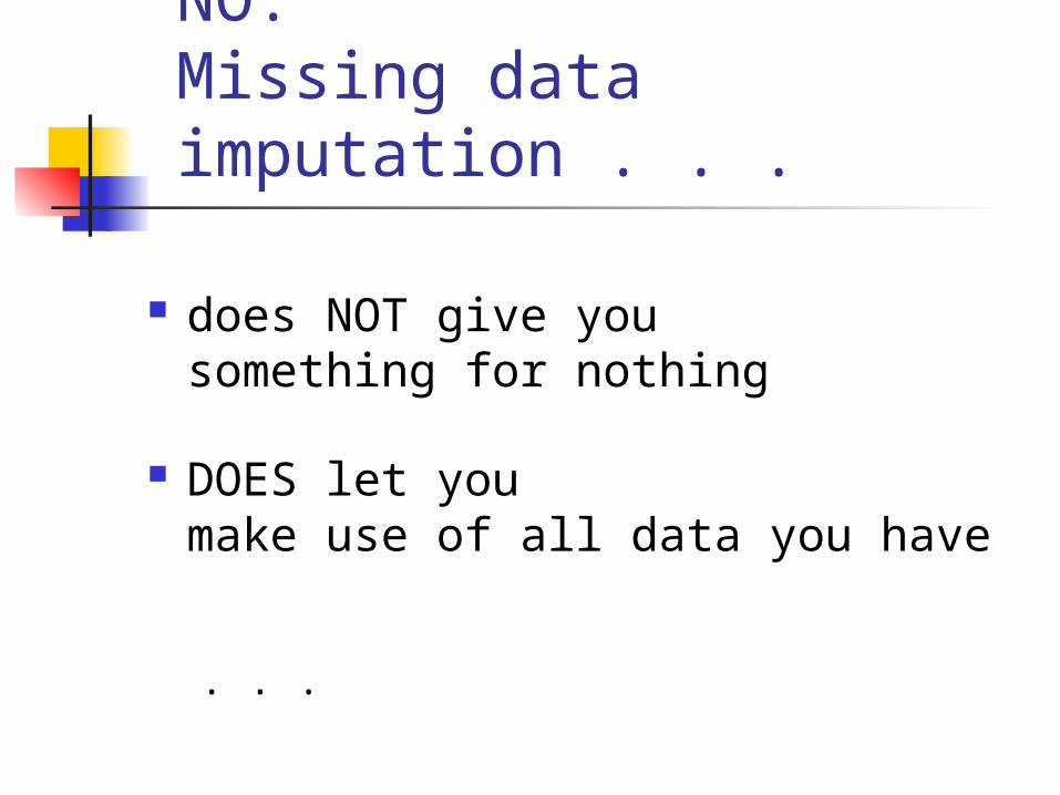
MCAR(Missing Completely At Random)
MCAR 1: Cause of missingness completely random process (like coin flip)
MCAR 2: Cause uncorrelated with variables of
interest Example: parents move
No bias if cause omitted

MAR (Missing At Random)
Missingness may be related to measured variables
But no residual relationship with unmeasured variables Example: reading speed
No bias if you control for measured variables

MNAR (Missing Not At Random)
Even after controlling for measured variables ...
Residual relationship with unmeasured variables
Example: drug use reason for absence

MNAR Causes
The recommended methods assume missingness is MAR
But what if the cause of missingness is not MAR?
Should these methods be used when MAR assumptions not met?
. . .

YES! These Methods Work!
Suggested methods work better than “old” methods
Multiple causes of missingness Only small part of missingness may be
MNAR
Suggested methods usually work very well

Revisit Question: What if THE Cause of Missingness is MNAR?
Example model of interest: X Y X = Program (prog vs control)Y = Cigarette SmokingZ = Cause of missingness: say,
Rebelliousness (or smoking itself) Factors to be considered:
% Missing (e.g., % attrition) rYZ . rZ,Ymis .
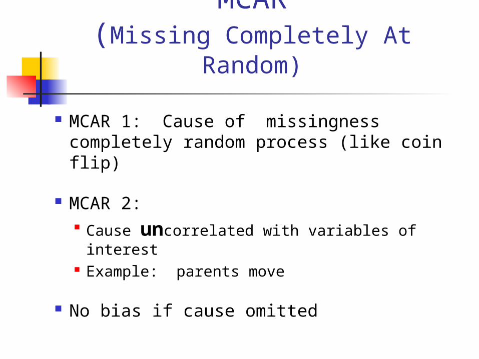
rYZ
Correlation between cause of missingness (Z)
e.g., rebelliousness (or smoking itself) and the variable of interest (Y)
e.g., Cigarette Smoking

rZ,Ymis
Correlation between cause of missingness (Z)
e.g., rebelliousness (or smoking itself) and missingness on variable of interest
e.g., Missingness on the Smoking variable
Missingness on Smoking (Ymis) Dichotomous variable:
Ymis = 1: Smoking variable not missing
Ymis = 0: Smoking variable missing

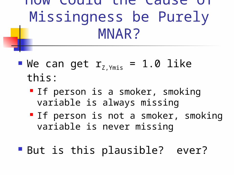
How Could the Cause of Missingness be Purely
MNAR?
rZ,Y = 1.0 AND rZ,Ymis = 1.0
We can get rZ,Y = 1.0 if smoking is the cause of missingness on the smoking variable
How Could the Cause of Missingness be Purely
MNAR?
We can get rZ,Ymis = 1.0 like this: If person is a smoker, smoking variable is
always missing If person is not a smoker, smoking
variable is never missing
But is this plausible? ever?

What if the cause of missingness is MNAR?
Problems with this statement
MAR & MNAR are widely misunderstood concepts
I argue that the cause of missingness is never purely MNAR
The cause of missingness is virtually never purely MAR either.
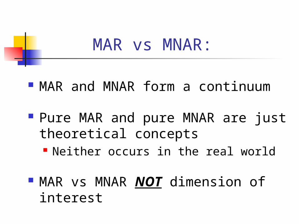
MAR vs MNAR:
MAR and MNAR form a continuum
Pure MAR and pure MNAR are just theoretical concepts Neither occurs in the real world
MAR vs MNAR NOT dimension of interest

MAR vs MNAR: What IS the Dimension of Interest?
Question of Interest:
How much estimation bias? when cause of missingness cannot be
included in the model
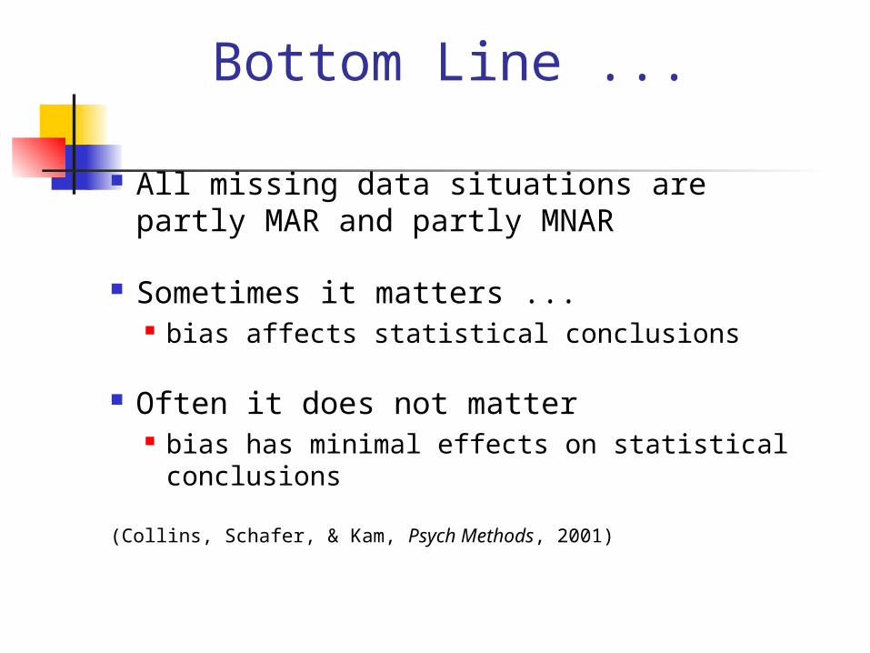
Bottom Line ...
All missing data situations are partly MAR and partly MNAR
Sometimes it matters ... bias affects statistical conclusions
Often it does not matter bias has minimal effects on statistical
conclusions
(Collins, Schafer, & Kam, Psych Methods, 2001)

Methods:"Old" vs MAR vs MNAR
MAR methods (MI and ML) are ALWAYS at least as good as, usually better than "old" methods
(e.g., listwise deletion)
Methods designed to handle MNAR missingness are NOT always better than MAR methods

References Graham, J. W., & Donaldson, S. I. (1993). Evaluating
interventions with differential attrition: The importance of nonresponse mechanisms and use of followup data. Journal of Applied Psychology, 78, 119-128.
Graham, J. W., Hofer, S.M., Donaldson, S.I., MacKinnon, D.P., & Schafer, J.L. (1997). Analysis with missing data in prevention research. In K. Bryant, M. Windle, & S. West (Eds.), The science of prevention: methodological advances from alcohol and substance abuse research. (pp. 325-366). Washington, D.C.: American Psychological Association.
Collins, L. M., Schafer, J. L., & Kam, C. M. (2001). A comparison of inclusive and restrictive strategies in modern missing data procedures. Psychological Methods, 6, 330-351.
Analysis: Old and New

Old Procedures: Analyze Complete
Cases(listwise deletion)
may produce bias
you always lose some power (because you are throwing away data)
reasonable if you lose only 5% of cases
often lose substantial power
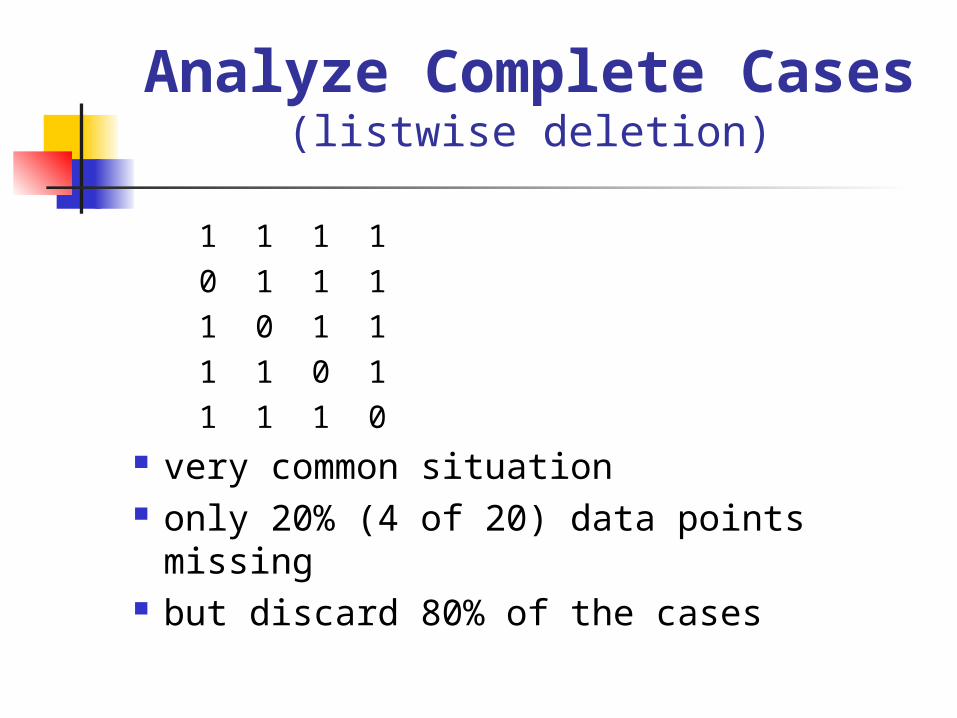
Analyze Complete Cases
(listwise deletion)
1 1 1 1 0 1 1 1 1 0 1 1 1 1 0 1 1 1 1 0
very common situation only 20% (4 of 20) data points missing but discard 80% of the cases
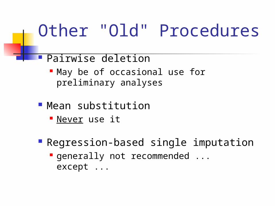
Other "Old" Procedures Pairwise deletion
May be of occasional use for preliminary analyses
Mean substitution Never use it
Regression-based single imputation generally not recommended ... except ...

Recommended Model-Based Procedures
Multiple Group SEM (Structural Equation Modeling)
Latent Transition Analysis (Collins et al.)
A latent class procedure

Recommended Model-Based Procedures
Raw Data Maximum Likelihood SEMaka Full Information Maximum Likelihood (FIML) Amos (James Arbuckle)
LISREL 8.5+ (Jöreskog & Sörbom)
Mplus (Bengt Muthén)
Mx (Michael Neale)
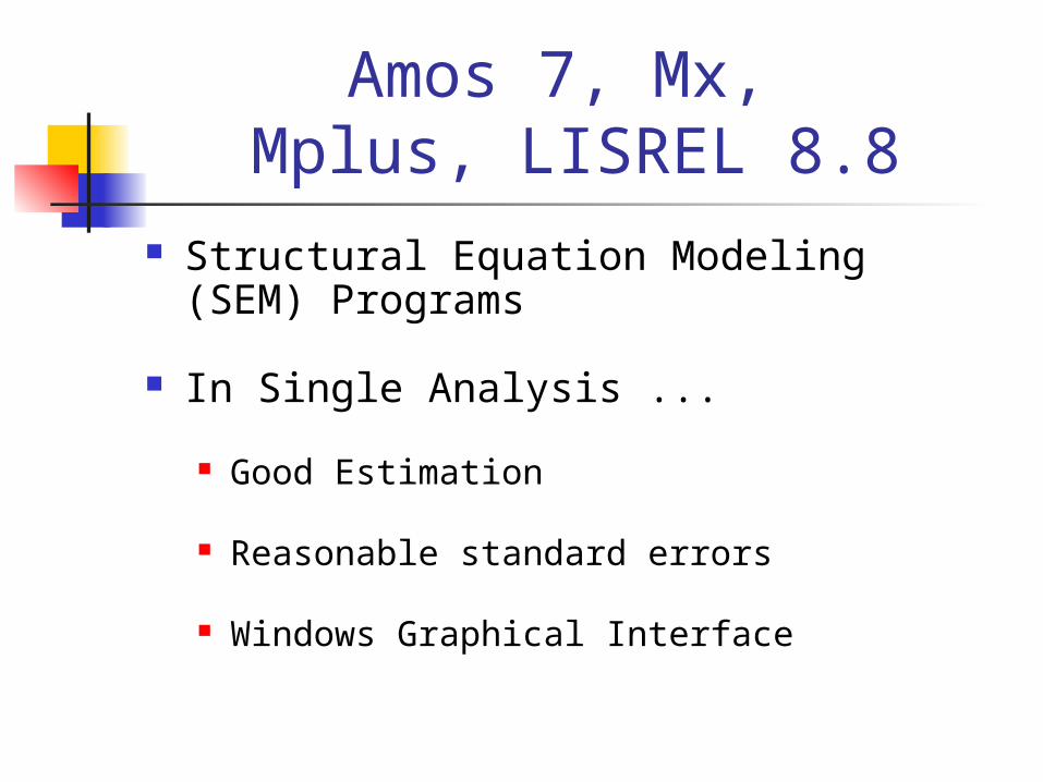
Amos 7, Mx, Mplus, LISREL 8.8
Structural Equation Modeling (SEM) Programs
In Single Analysis ...
Good Estimation
Reasonable standard errors
Windows Graphical Interface
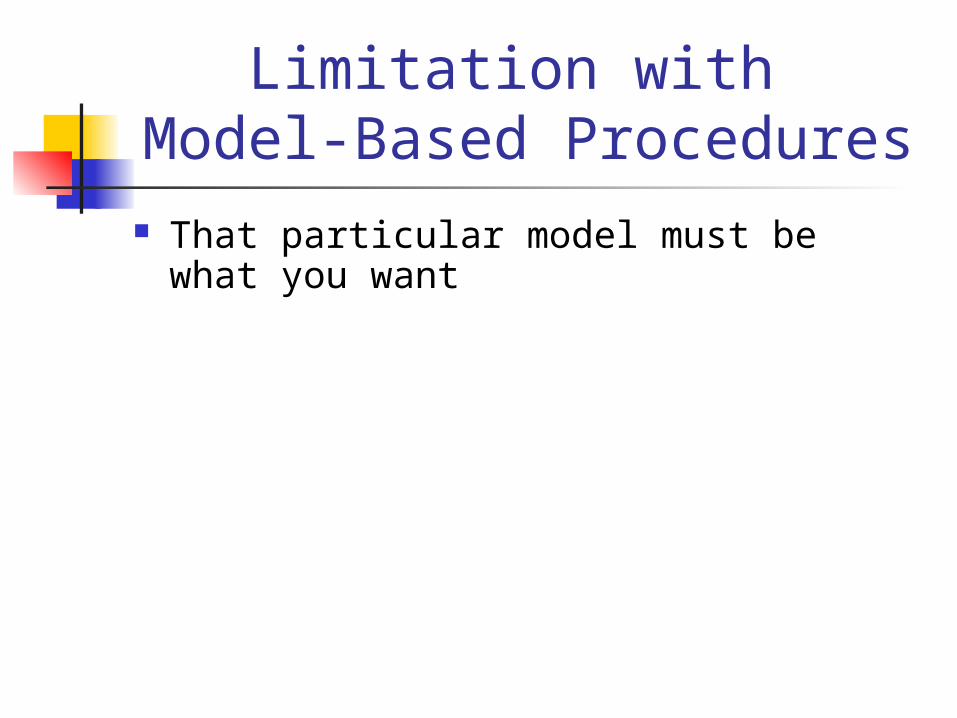
Limitation with Model-Based Procedures
That particular model must be what you want

Recommended Data-Based Procedures
EM Algorithm (ML parameter estimation)
Norm-Cat-Mix, EMcov, SAS, SPSS
Multiple Imputation NORM, Cat, Mix, Pan (Joe Schafer) SAS Proc MI LISREL 8.5+

EM Algorithm Expectation - MaximizationAlternate between
E-step: predict missing dataM-step: estimate parameters
Excellent parameter estimates
But no standard errors must use bootstrap or multiple imputation
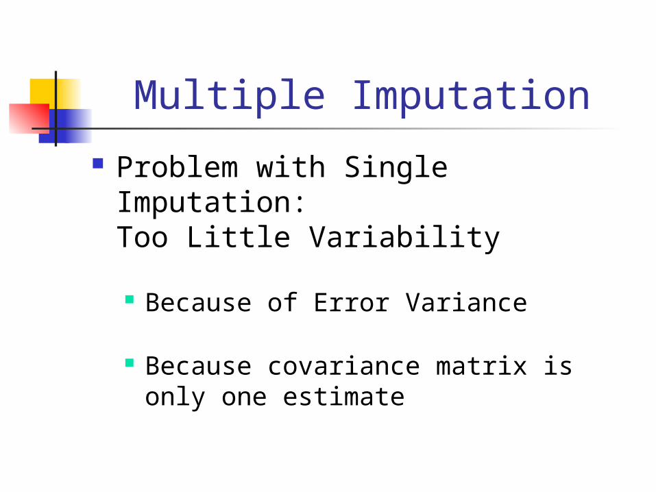
Multiple Imputation
Problem with Single Imputation:Too Little Variability
Because of Error Variance
Because covariance matrix is only one estimate
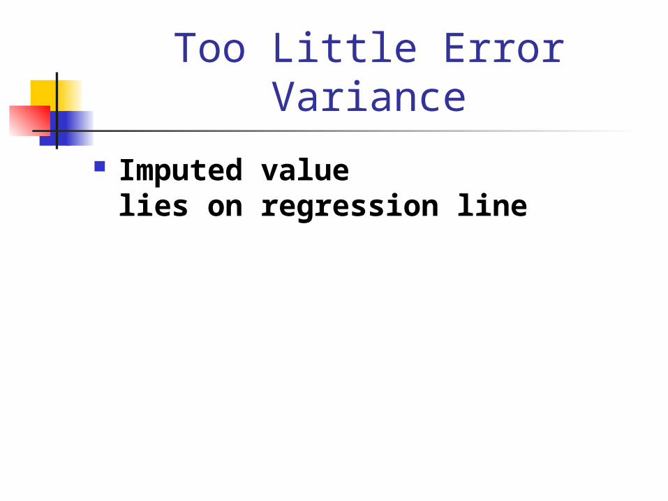
Too Little Error Variance
Imputed value lies on regression line

Imputed Values on Regression Line
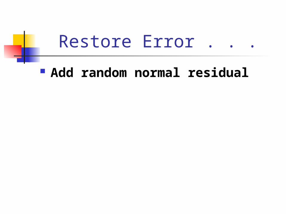
Restore Error . . .
Add random normal residual

Covariance Matrix (Regression Line) only One
Estimate Obtain multiple plausible estimates of the
covariance matrix
ideally draw multiple covariance matrices from population
Approximate this with Bootstrap Data Augmentation (Norm) MCMC (SAS 8.2, 9)
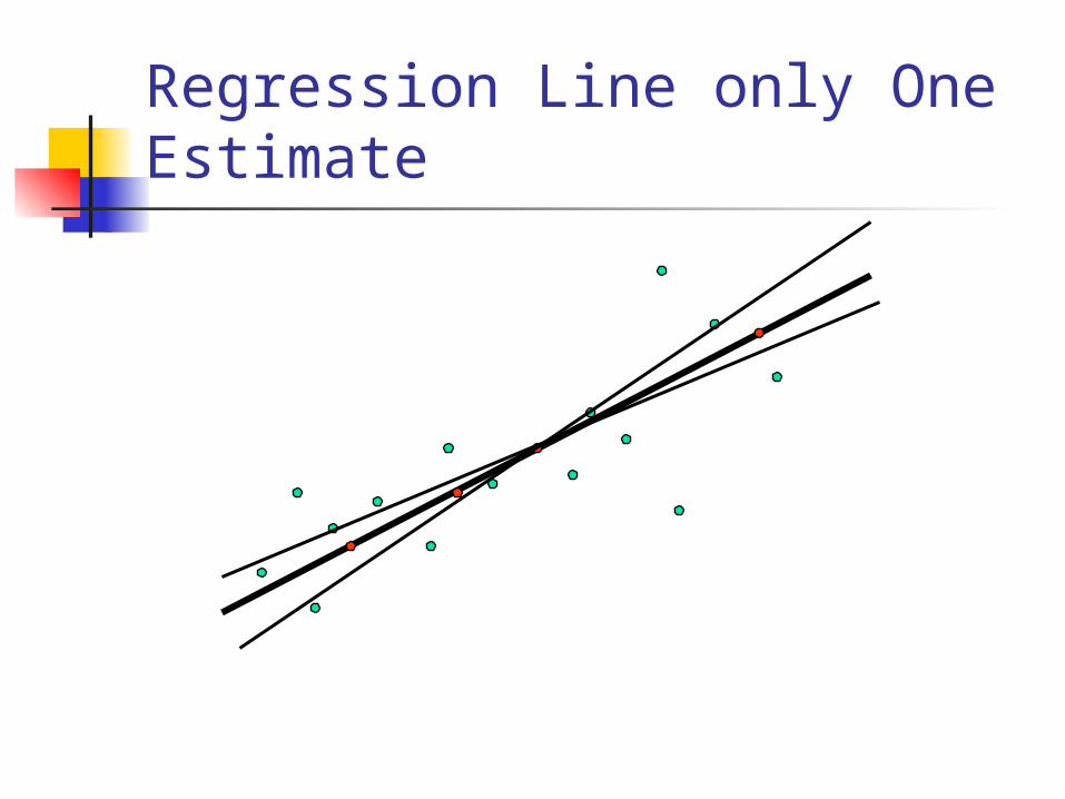
Regression Line only One Estimate

Data Augmentation stochastic version of EM
EM E (expectation) step: predict missing data M (maximization) step: estimate parameters
Data Augmentation I (imputation) step: simulate missing data P (posterior) step: simulate parameters

Data Augmentation
Parameters from consecutive steps ... too related i.e., not enough variability
after 50 or 100 steps of DA ...
covariance matrices are like random draws from the population

Multiple Imputation Allows:
Unbiased Estimation
Good standard errors provided number of imputations is
large enough too few imputations reduced power
with small effect sizes

0
2
4
6
8
10
12
14
Perc
ent P
ow
er
Fallo
ff
100 85 70 55 40 25 10m Imputations
Power FalloffFMI = .50, rho = .10
From Graham, J. W., Olchowski, A. E., & Gilreath, T. D. (in press). How many imputations are really needed? Some practical clarifications of multiple imputation theory.
Prevention Science.

Part II:Illustration of Missing Data
Analysis: Multiple Imputation with NORM and
Proc MI
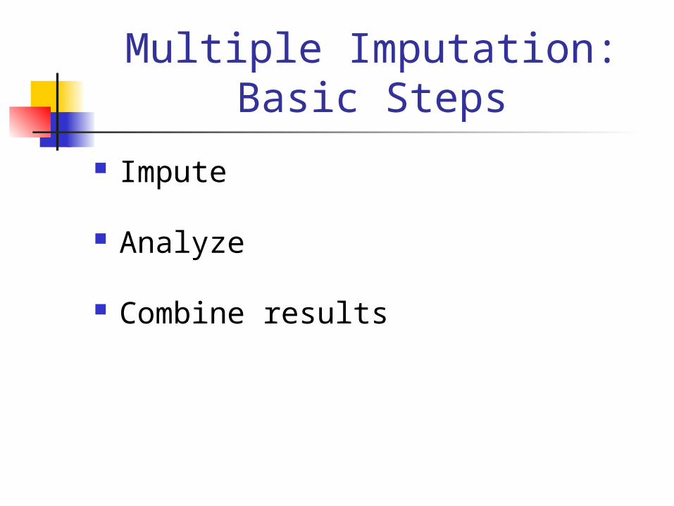
Multiple Imputation:Basic Steps
Impute
Analyze
Combine results

Imputation and Analysis
Impute 40 datasets a missing value gets a different imputed
value in each dataset
Analyze each data set with USUAL procedures e.g., SAS, SPSS, LISREL, EQS, STATA
Save parameter estimates and SE’s
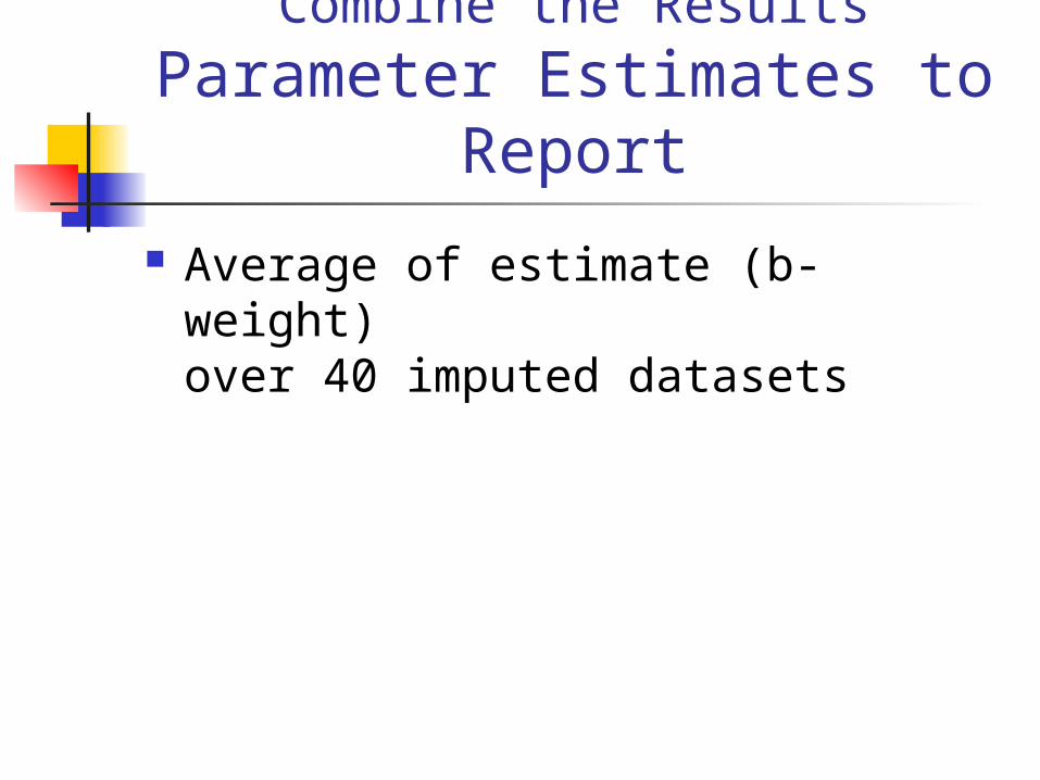
Combine the ResultsParameter Estimates to
Report
Average of estimate (b-weight) over 40 imputed datasets

Combine the ResultsStandard Errors to Report
Sum of: “within imputation” variance
average squared standard error usual kind of variability
“between imputation” variancesample variance of parameter estimates
over 40 datasets variability due to missing data

Materials for SPSS Regression
Starting place http://methodology.psu.edu
downloads missing data software Joe Schafer's Missing Data Programs John Graham's Additional NORM Utilities
http://mcgee.hhdev.psu.edu/missing/index.html
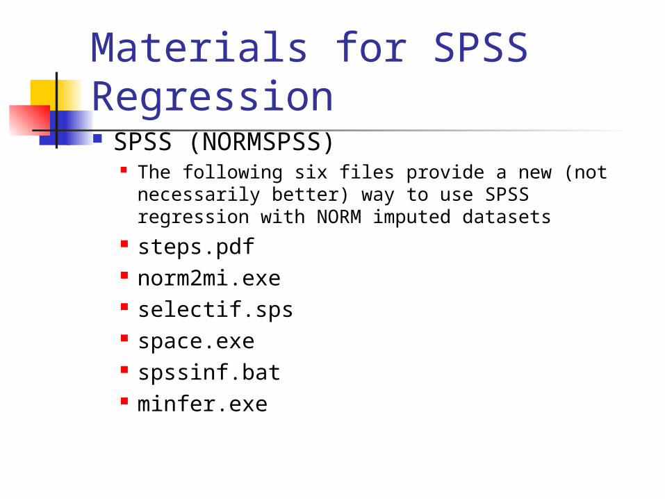
Materials for SPSS Regression SPSS (NORMSPSS)
The following six files provide a new (not necessarily better) way to use SPSS regression with NORM imputed datasets
steps.pdf norm2mi.exe selectif.sps space.exe spssinf.bat minfer.exe

exit for sample analysis

Inclusive Missing Data Strategies
Auxiliary Variables:
What’s All the Fuss?
John GrahamIES Summer Research Training Institute, June 27, 2007

What Is an Auxiliary Variable?
A variable correlated with the variables in your modelbut not part of the modelnot necessarily related to missingnessused to "help" with missing data estimation

Benefit of Auxiliary Variables
Collins, L. M., Schafer, J. L., & Kam, C. M. (2001). A comparison of inclusive and restrictive strategies in modern missing data procedures. Psychological Methods, 6, 330_351.
Graham, J. W., & Collins, L. M. (2007). Using modern missing data methods with auxiliary variables to mitigate the effects of attrition on statistical power. Technical Report, The Methodology Center, Penn State University.
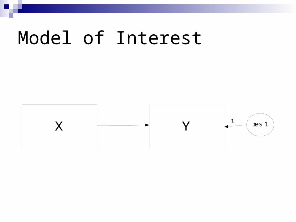
Model of Interest
X Y res 11

Benefit of Auxiliary Variables
Example from Graham & Collins (2007)
X Y Z
1 1 1 500 complete cases
1 0 1 500 cases missing Y
X, Y variables in the model (Y sometimes missing)
Z is auxiliary variable

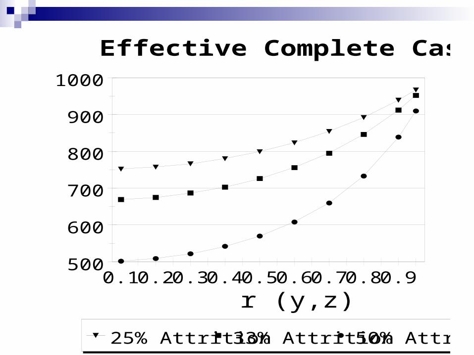
Benefit of Auxiliary Variables
Effective sample size (N')
Analysis involving N cases, with auxiliary variable(s)
gives statistical power equivalent to N' complete cases without auxiliary variables

Benefit of Auxiliary Variables It matters how highly Y and Z (the auxiliary
variable) are correlated
For exampleincrease
rYZ = .40 N = 500 gives power of N' = 542 (8%)
rYZ = .60 N = 500 gives power of N' = 608 (22%)
rYZ = .80 N = 500 gives power of N' = 733 (47%)
rYZ = .90 N = 500 gives power of N' = 839 (68%)
500
600
700
800
900
1000
0.1 0.2 0.3 0.4 0.5 0.6 0.7 0.8 0.9
r (y,z)
25% Attrition 33% Attrition 50% Attrition
Effective Complete Cases N

Empirical IllustrationThe Model
Alcohol-related Harm Prevention (AHP) Project with College Students
Intent make Vehicle Plans
1
Alcohol Use1
Took VehicleRisks 3
PhysicalHarm 5

How Much Data? Intent Alcohol VehRisk Harm Freq
_______ ____ ____ ______ ____
0 0 0 0 59
0 0 0 1 109
0 0 1 0 99
0 0 1 1 122
0 1 0 0 1
0 1 0 1 2
0 1 1 1 5
1 1 0 0 100
1 1 0 1 46
1 1 1 0 136
1 1 1 1 344 Complete
Total 1023
1 = data0 = missing
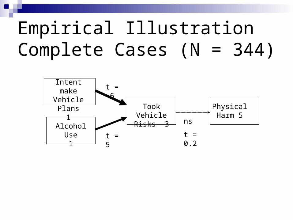
Empirical IllustrationComplete Cases (N = 344)
Intent make Vehicle Plans
1
Alcohol Use1
Took VehicleRisks 3
PhysicalHarm 5
ns
t = 0.2
t = -6
t = 5

Empirical IllustrationSimple MI (no Aux Vars)
Intent make Vehicle Plans
1
Alcohol Use1
Took VehicleRisks 3
PhysicalHarm 5
t = 3
t = -9
t = 7
N = 1023

Empirical IllustrationMI with Aux Vars
Intent make Vehicle Plans
1
Alcohol Use1
Took VehicleRisks 3
PhysicalHarm 5
t = 6
t = -10
t = 8
N = 1023
Auxiliary Variables:
Intent2, Intent3, Intent4, Intent5Alcohol2, Alcohol3, Alcohol4, Alcohol5Risks1, Risks3, Risks4, Risks5Harm1, Harm2, Harm3, Harm4

Effect of Auxiliary Variables onFraction of Missing Information
no aux vars
16 aux vars
iplnvsep harm2nv0 .71 .46
alcsep harm2nv0 .64 .44
female harm2nv0 .48 .27
vriskfeb harm2nv0 .85 .67iplnvsep harm2nv0 .76 .53
alcsep harm2nv0 .68 .46
female harm2nv0 .52 .27
iplnvsep vriskfeb .58 .46
alcsep vriskfeb .56 .32female vriskfeb .42 .28

Methods for Adding Auxiliary Variables
Multiple Imputation
Amos

Adding Auxiliary Variables: MI
Simply add Auxiliary variables to imputation model
Couldn't be easierExcept ... There are limits to how many variables can be
included in NORM conveniently My current thinking:
add Aux Vars judiciously

Empirical IllustrationMI with Aux Vars
Intent make Vehicle Plans
1
Alcohol Use1
Took VehicleRisks 3
PhysicalHarm 5
t = 6
t = -10
t = 8
N = 1023
Auxiliary Variables:
Intent2, Intent3, Intent4, Intent5Alcohol2, Alcohol3, Alcohol4, Alcohol5Risks1, Risks3, Risks4, Risks5Harm1, Harm2, Harm3, Harm4

Adding Auxiliary Variables: Amos (and other FIML/SEM programs)
Graham, J. W. (2003). Adding missing-data relevant variables to FIML-based structural equation models. Structural Equation Modeling, 10, 80-100.
Extra DV model Good for manifest variable models
Saturated Correlates ("Spider") ModelBetter for latent variable models

Covariate Model
0,
X
X1
0,
e1
1
1
X2
0,
e21
X3
0,
e31
X4
0,
e41
0
Y
Y1
0,
e5
Y2
0,
e6
Y3
0,
e7
Y4
0,
e8
1
1 1 1 1
0,
resid1
1
Aux NOT Adequate
Aux Variable Changes XY Estimate

Extra DV Model
X Y
Aux
res 11
res 21
Good for Manifest Variable Models
Aux Variable does NOT Change XY Estimate

Spider Model (Graham, 2003)
0,
X
X1
0,
e1
1
1
X2
0,
e21
X3
0,
e31
X4
0,
e41
0
Y
Y1
0,
e5
Y2
0,
e6
Y3
0,
e7
Y4
0,
e8
1
1 1 1 1
RX3
0,
resid1
1
Good for Latent Variable ModelsAux Variable does NOT Change XY Estimate
Aux

Extra DV Model (Amos)
iplnvsepharm2nv0
0,
res1
1vriskfeb
0,
r21
female
alcsep
iplnvnoviplnvfebiplnvapriplnvnv0alcnovalcfebalcapralcnv0
vrisksepvrisknovvriskaprvrisknv0
harm2sepharm2novharm2febharm2apr
0,e1
10,
e21
0,e3
10,
e41
0,e5
10,
e61
0,e7
10,
e81
0,e9
10,
e101
0,e11
10,
e121
0,e13
10,
e141
0,e15
10,
e161
Real world version gets a little clumsy ...
but Amos does provide some excellent drawing tools
Large models easier in text-based SEM programs (e.g., LISREL)

Using Missing Data Analysis and Design to Develop Cost-
Effective Measurement Strategies in Prevention
Research
John Graham
IES Summer Research Training Institute, June 27, 2007

Planned Missingness Designs:
The 3-Form Design

Planned Missingness
Why would anyone want to plan to have missing data?
To manage costs, data quality, and statistical power
In fact, we've been doing it for decades
. . .
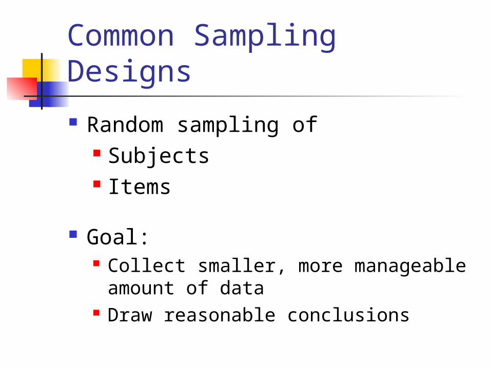
Common Sampling Designs
Random sampling of Subjects Items
Goal: Collect smaller, more manageable
amount of data Draw reasonable conclusions
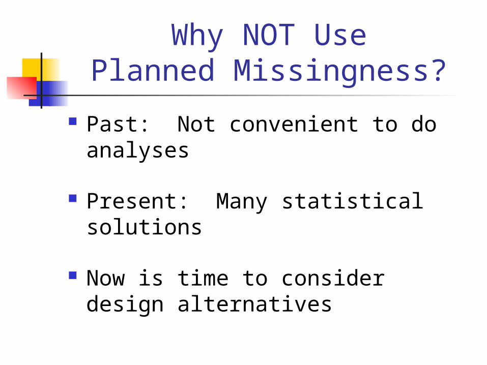
Why NOT UsePlanned Missingness?
Past: Not convenient to do analyses
Present: Many statistical solutions
Now is time to consider design alternatives

Design Examples

Lighten Burden on Respondents
The problem: 7th graders can answer only 100
questions
We want to ask 133 questions
One Solution: The 3-form design

Idea Grew out of Practical Need
Project SMART (1982) NIDA-funded drug abuse prevention
project Johnson, Flay, Hansen, Graham

3-Form Design
Student Received Item Set?----------------------------X A B C
Form 1 yes yes yes NOForm 2 yes yes NO yesForm 3 yes NO yes yes

3-Form Design
Item Sets totalX A B C asked34 33 33 33 = 133
totalfor each
form X A B C student1 34 33 33 0 = 1002 34 33 0 33 = 1003 34 0 33 33 = 100
Think of it as “leveraging” resources
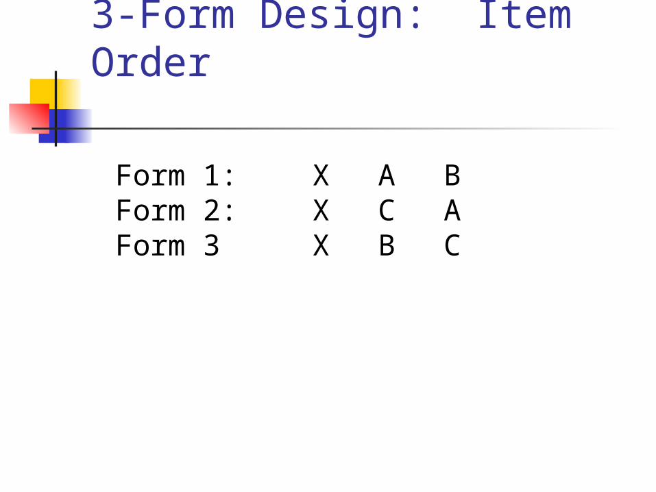
3-Form Design: Item Order
Form 1: X A BForm 2: X C AForm 3 X B C

3-Form Design: Item Order
Form 1: X A B CForm 2: X C A BForm 3 X B C A

3-Form Design: Item Order
Form 1: X A B CForm 2: X C A BForm 3 X B C A
Give questions as shown, measure reasons for non-completion poor reading low motivation conscientiousness
"Managed" missingness

Other Designs in the Same Family

3-Form Design(Graham, Flay et al., 1984)
Item SetsX A B C total
Form 33 33 33 33 133_____ _____________________________________
1 33 33 33 0 1002 33 33 0 33 1003 33 0 33 33 100
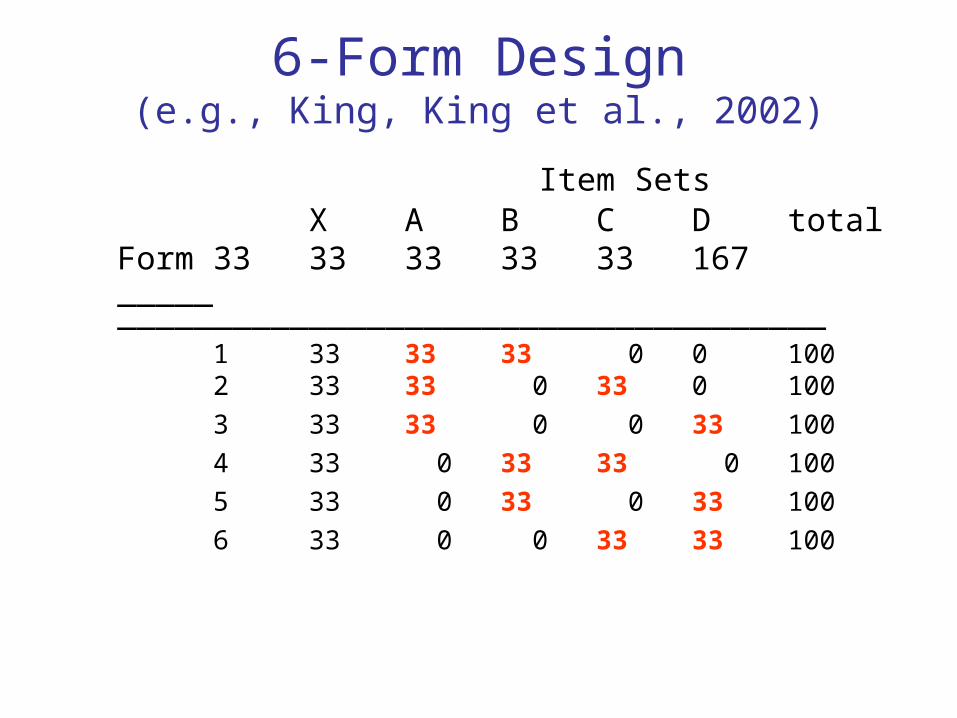
6-Form Design(e.g., King, King et al., 2002)
Item SetsX A B C D total
Form 33 33 33 33 33 167_____ _____________________________________
1 33 33 33 0 0 1002 33 33 0 33 0 1003 33 33 0 0 33 1004 33 0 33 33 0 1005 33 0 33 0 33 1006 33 0 0 33 33 100
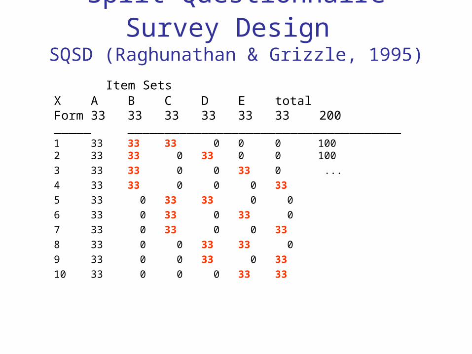
Split Questionnaire Survey Design
SQSD (Raghunathan & Grizzle, 1995)
Item SetsX A B C D E total
Form 33 33 33 33 33 33 200_____ _____________________________________
1 33 33 33 0 0 0 1002 33 33 0 33 0 0 100
3 33 33 0 0 33 0 ...
4 33 33 0 0 0 33
5 33 0 33 33 0 0
6 33 0 33 0 33 0
7 33 0 33 0 0 33
8 33 0 0 33 33 0
9 33 0 0 33 0 33
10 33 0 0 0 33 33

Family of Designs
3-form Design All combinations of 3 sets taken 2 at a time
SQSD (10-form design) All combinations of 5 sets taken 2 at a time
6-form design All combinations of 4 sets taken 2 at a time
Complete cases (1-form design) All combinations of 2 sets taken 2 at a time

Evaluating Designs (Benefits and costs)

Evaluating Designs (Benefits and costs)
Number of item sets (4 vs 3)Number of items (133 vs 100)
Number of (correlation) effectsSample sizes
.....

Number of
Effects
Effects tested with
n = N/3 (100)
Effects tested with
n = 2N/3 (200)
Effects tested with
total N (300)
Effects tested with
total N (300)

Evaluating Designs (Benefits and costs)
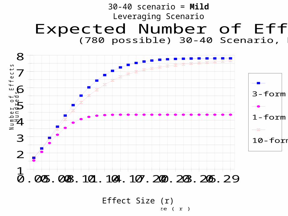
Number of effects tested with good power (power ≥ .80)
Take multiple effect sizes into account
1
2
3
4
5
6
7
8
Nu
mb
er
of
Eff
ects
Hu
nd
red
s
0.050.080.110.140.170.200.230.260.29
Effect Size ( r )
3-form
1-form
10-form
Expected Number of Effects Detected(780 possible) 30-40 Scenario, N=1000
Effect Size (r)
30-40 scenario = Mild Leveraging Scenario

Evaluating Designs (Benefits and costs)
Number of effects tested with good power (power ≥ .80) …Still Something Missing
It's not how many effects
But WHICH effects can be tested:
Tradeoff Matrix
S T U D Y N = 1 0 0 0Effects
XA, XBEffect XX AA, BB AB XC, CC AC, BC
Size (r) 1-form(1000)
3-form(1000)
1-form(1000)
3-form(667)
1-form(1000)
3-form(333)
1-form(0)
3-form(667)
1-form(0)
3-form(333)
0.05 .35 .35 .35 .25 .35 .15 0 .25 0 .150.06 .48 .48 .48 .34 .48 .19 0 .34 0 .190.07 .60 .60 .60 .44 .60 .25 0 .44 0 .250.08 .72 .72 .72 .54 .72 .31 0 .54 0 .310.09 .81 .81 .81 .64 .81 .38 0 .64 0 .380.10 .89 .89 .89 .74 .89 .45 0 .74 0 .450.11 .94 .94 .94 .81 .94 .52 0 .81 0 .520.12 .97 .97 .97 .88 .97 .59 0 .88 0 .590.13 .99 .99 .99 .92 .99 .66 0 .92 0 .660.14 .99 .99 .99 .95 .99 .73 0 .95 0 .730.15 ** ** ** .97 ** .79 0 .97 0 .79 0.16 ** ** ** .99 ** .84 0 .99 0 .84 0.17 ** ** ** .99 ** .88 0 .99 0 .88 0.18 ** ** ** ** ** .91 0 ** 0 .91 0.19 ** ** ** ** ** .94 0 ** 0 .94 0.20 ** ** ** ** ** .96 0 ** 0 .96 0.21 ** ** ** ** ** .97 0 ** 0 .97 0.22 ** ** ** ** ** .98 0 ** 0 .98 0.23 ** ** ** ** ** .99 0 ** 0 .99 0.24 ** ** ** ** ** .99 0 ** 0 .99 0.25 ** ** ** ** ** ** 0 ** 0 ** 0.26 ** ** ** ** ** ** 0 ** 0 ** 0.27 ** ** ** ** ** ** 0 ** 0 ** 0.28 ** ** ** ** ** ** 0 ** 0 ** 0.29 ** ** ** ** ** ** 0 ** 0 ** 0.30 ** ** ** ** ** ** 0 ** 0 ** ** power > .995
1.271.20
2.13
1.36
powerratio

3-Form Design
Student Received Item Set?----------------------------X A B Ccore peer parent other
Form 1 yes yes yes NOForm 2 yes yes NO yesForm 3 yes NO yes yes

3-Form Design:Implementation Strategies
Core Questions in "X" set Keep related questions together
in A or B or C sets Example for Collaboration
(Hansen & Graham) X set (core items)
A: Hansen Set B: Graham set C: Other

"Back Against the Wall" Concept
3-form design better received if one of these is true:
You CAN ask some number of questions (e.g., 100) You WANT to ask some larger number of
questions (e.g., 133) You have been asking 133 questions of
respondents Data Collectors (or data gate keepers) say you
MUST reduce number of questions
Some Future Directions Current power calculations based
on zero-order correlations (beneficial) effect of auxiliary
variables not taken into account
Current power calculations based on level one correlation analysis loss of power will be discounted in
multilevel analyses

Change in FMI adding 15 Aux Vars from X set
Predictors FMI change r with Aux Vars
posatt .48 .30 .54
freetimewithfriends .47 .34 .29
fangry .49 .38 .56
nparties .41 .33 .36
negatt .46 .37 .26
sportsimportant .47 .39 .16
nclosefriends .46 .40 .20
carefriends .46 .43 .28
parangry .39 .38 .45
easytalkfriends .43 .43 .24DV: Trouble Dataset: AAPT 7th graders

the end