Embed Size (px)
Citation preview
MIT 2.853/2.854Introduction to Manufacturing
SystemsMaterial Requirements Planning
Lecturer: Stanley B. Gershwin
Copyright c©2002-2006 Stanley B. Gershwin.
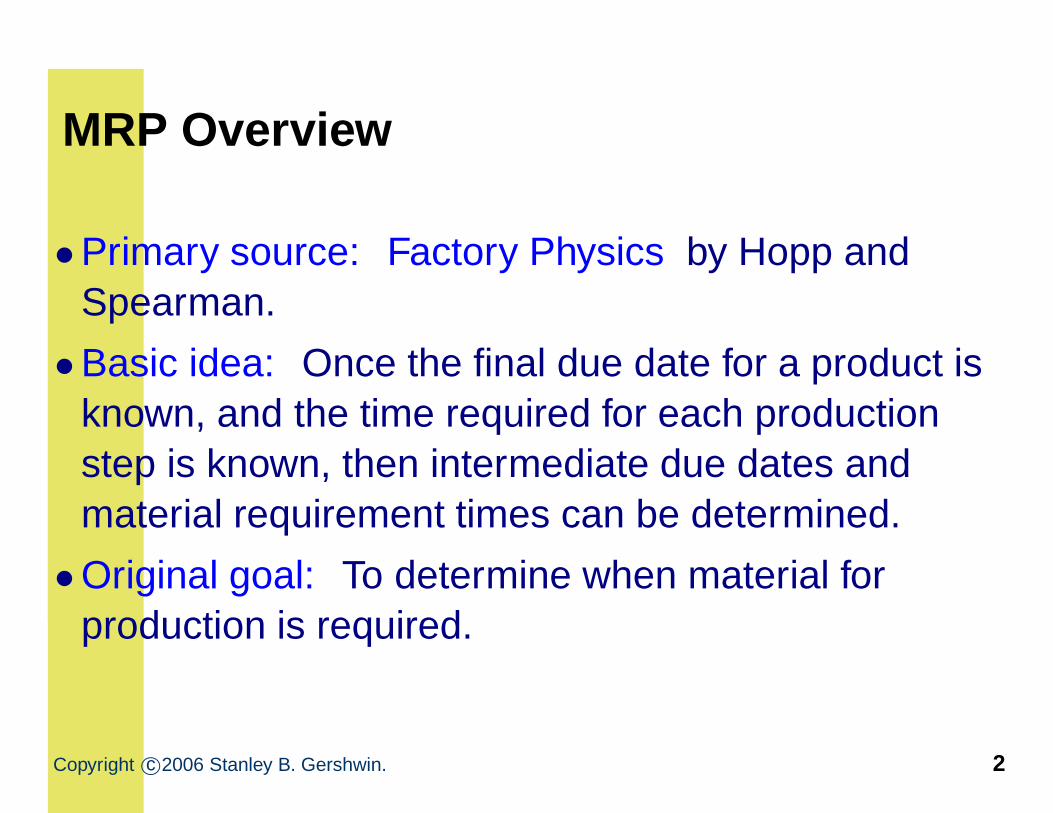
MRP Overview
•Primary source: Factory Physics by Hopp andSpearman.
•Basic idea: Once the final due date for a product isknown, and the time required for each productionstep is known, then intermediate due dates andmaterial requirement times can be determined.
•Original goal: To determine when material forproduction is required.
Copyright c©2006 Stanley B. Gershwin. 2
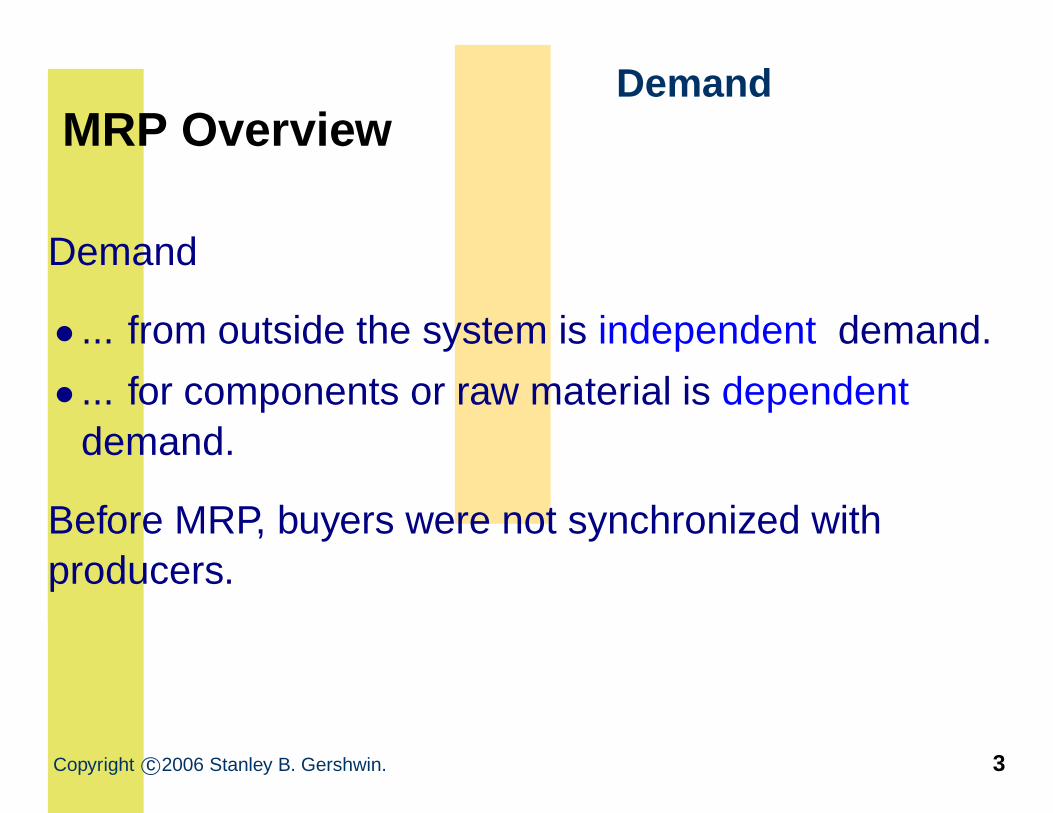
MRP OverviewDemand
Demand
• ... from outside the system is independent demand.
• ... for components or raw material is dependentdemand.
Before MRP, buyers were not synchronized withproducers.
Copyright c©2006 Stanley B. Gershwin. 3
MRP OverviewPlanning Algorithm
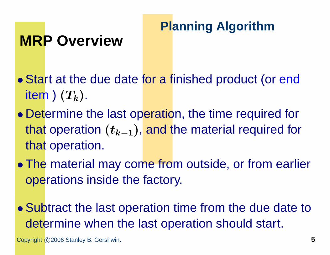
•Start at the due date for a finished product (or enditem ) (Tk).
•Determine the last operation, the time required forthat operation (tk−1), and the material required forthat operation.
•The material may come from outside, or from earlieroperations inside the factory.
•Subtract the last operation time from the due date todetermine when the last operation should start.
Copyright c©2006 Stanley B. Gershwin. 5
MRP OverviewPlanning Algorithm
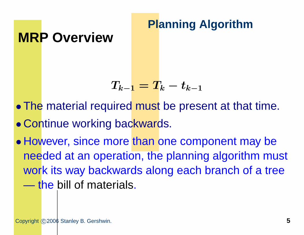
Tk−1 = Tk − tk−1
•The material required must be present at that time.
•Continue working backwards.
•However, since more than one component may beneeded at an operation, the planning algorithm mustwork its way backwards along each branch of a tree— the bill of materials.
Copyright c©2006 Stanley B. Gershwin. 5
MRP OverviewPlanning Algorithm
Time
• In some MRP systems, time is divided into timebuckets — days, weeks, or whatever is convenient.
• In others, time may be chosen as a continuousvariable.
Copyright c©2006 Stanley B. Gershwin. . 6
MRP OverviewDiscussion
•What assumptions are being made here ...
⋆ ... about predictability?⋆ ... about capacity?
•How realistic are those assumptions?
• Is it more flexible to use time buckets or continuoustime?
Copyright c©2006 Stanley B. Gershwin. 7
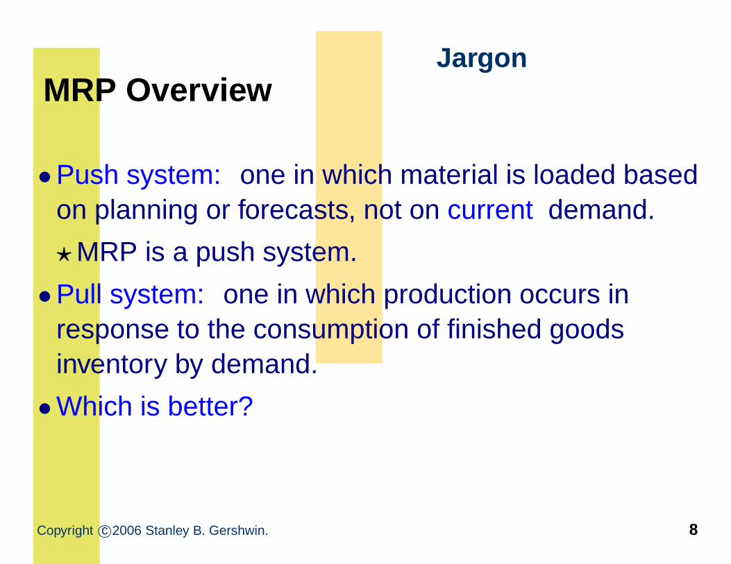
MRP OverviewJargon
•Push system: one in which material is loaded basedon planning or forecasts, not on current demand.
⋆MRP is a push system.
•Pull system: one in which production occurs inresponse to the consumption of finished goodsinventory by demand.
•Which is better?
Copyright c©2006 Stanley B. Gershwin. 8
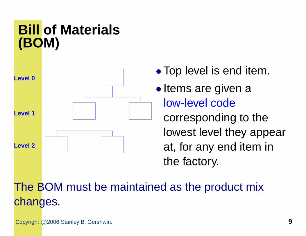
Bill of Materials(BOM)
Level 0
Level 1
Level 2
•Top level is end item.
• Items are given alow-level codecorresponding to thelowest level they appearat, for any end item inthe factory.
The BOM must be maintained as the product mixchanges.
Copyright c©2006 Stanley B. Gershwin. 9
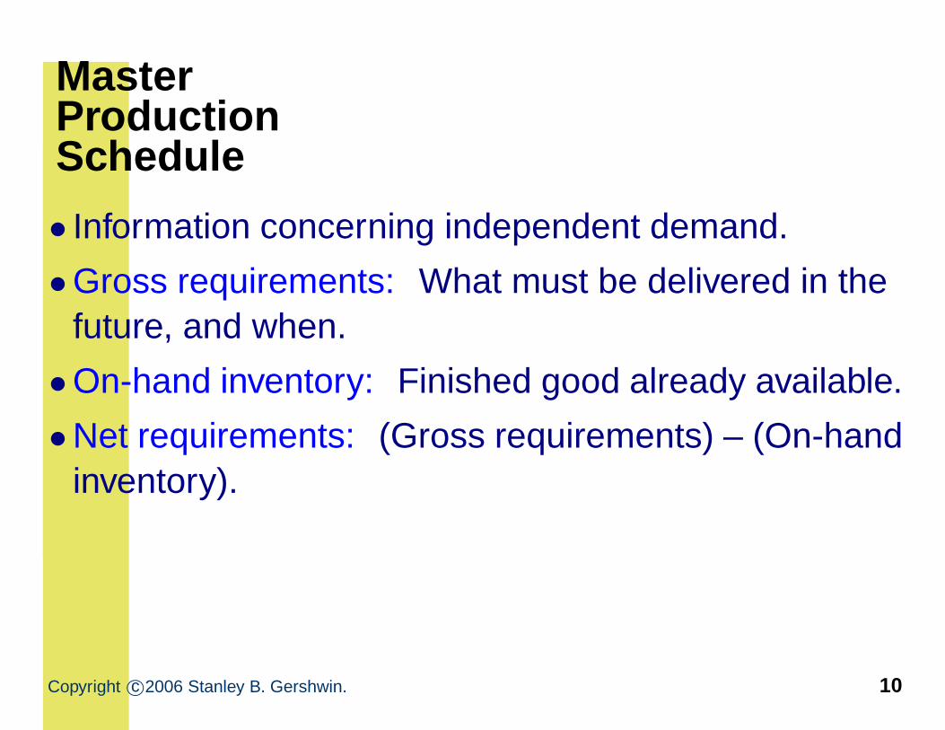
MasterProductionSchedule
• Information concerning independent demand.
•Gross requirements: What must be delivered in thefuture, and when.
•On-hand inventory: Finished good already available.
•Net requirements: (Gross requirements) – (On-handinventory).
Copyright c©2006 Stanley B. Gershwin. 10
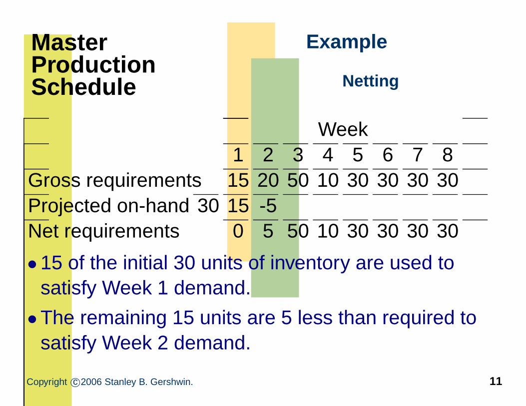
MasterProductionSchedule
Example
Netting
Week1 2 3 4 5 6 7 8
Gross requirements 15 20 50 10 30 30 30 30Projected on-hand 30 15 -5Net requirements 0 5 50 10 30 30 30 30
• 15 of the initial 30 units of inventory are used tosatisfy Week 1 demand.
•The remaining 15 units are 5 less than required tosatisfy Week 2 demand.
Copyright c©2006 Stanley B. Gershwin. 11
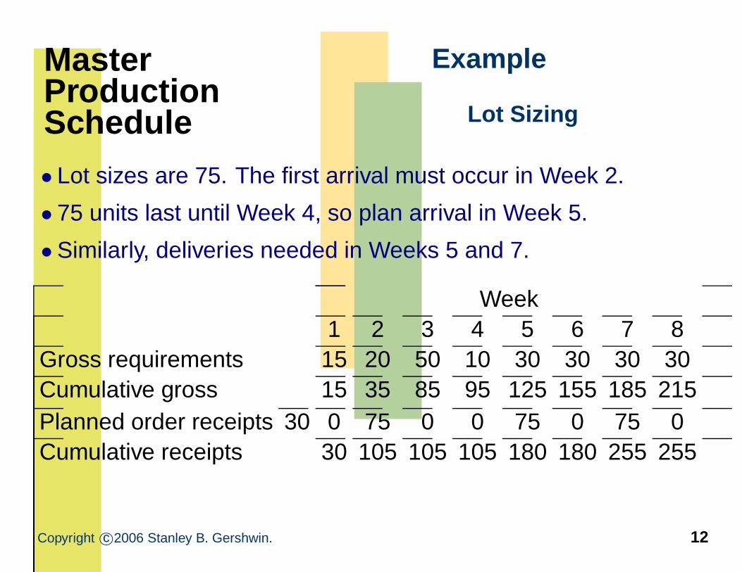
MasterProductionSchedule
Example
Lot Sizing
• Lot sizes are 75. The first arrival must occur in Week 2.
• 75 units last until Week 4, so plan arrival in Week 5.
• Similarly, deliveries needed in Weeks 5 and 7.
Week1 2 3 4 5 6 7 8
Gross requirements 15 20 50 10 30 30 30 30Cumulative gross 15 35 85 95 125 155 185 215Planned order receipts 30 0 75 0 0 75 0 75 0Cumulative receipts 30 105 105 105 180 180 255 255
Copyright c©2006 Stanley B. Gershwin. 12
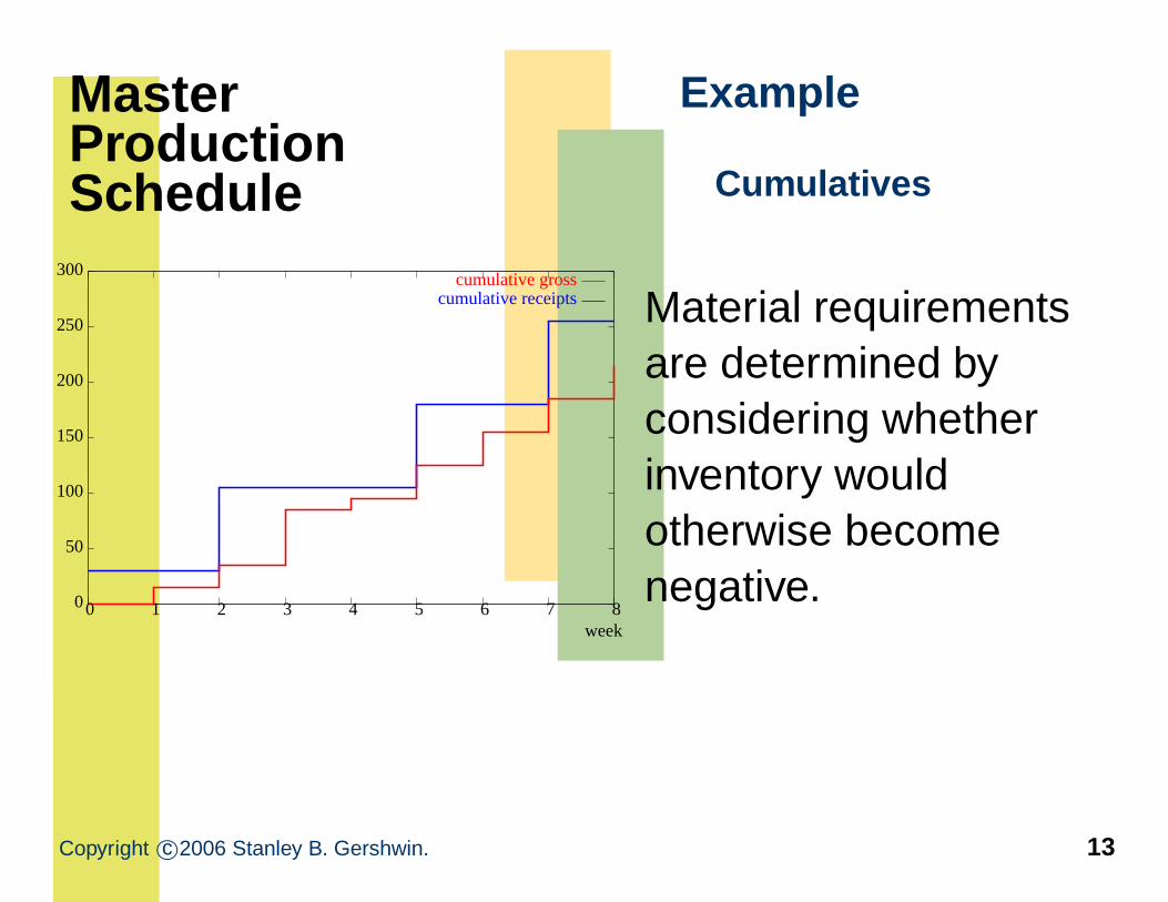
MasterProductionSchedule
Example
Cumulatives
0
50
100
150
200
250
300
0 1 2 3 4 5 6 7 8
cumulative grosscumulative receipts
week
Material requirementsare determined byconsidering whetherinventory wouldotherwise becomenegative.
Copyright c©2006 Stanley B. Gershwin. 13
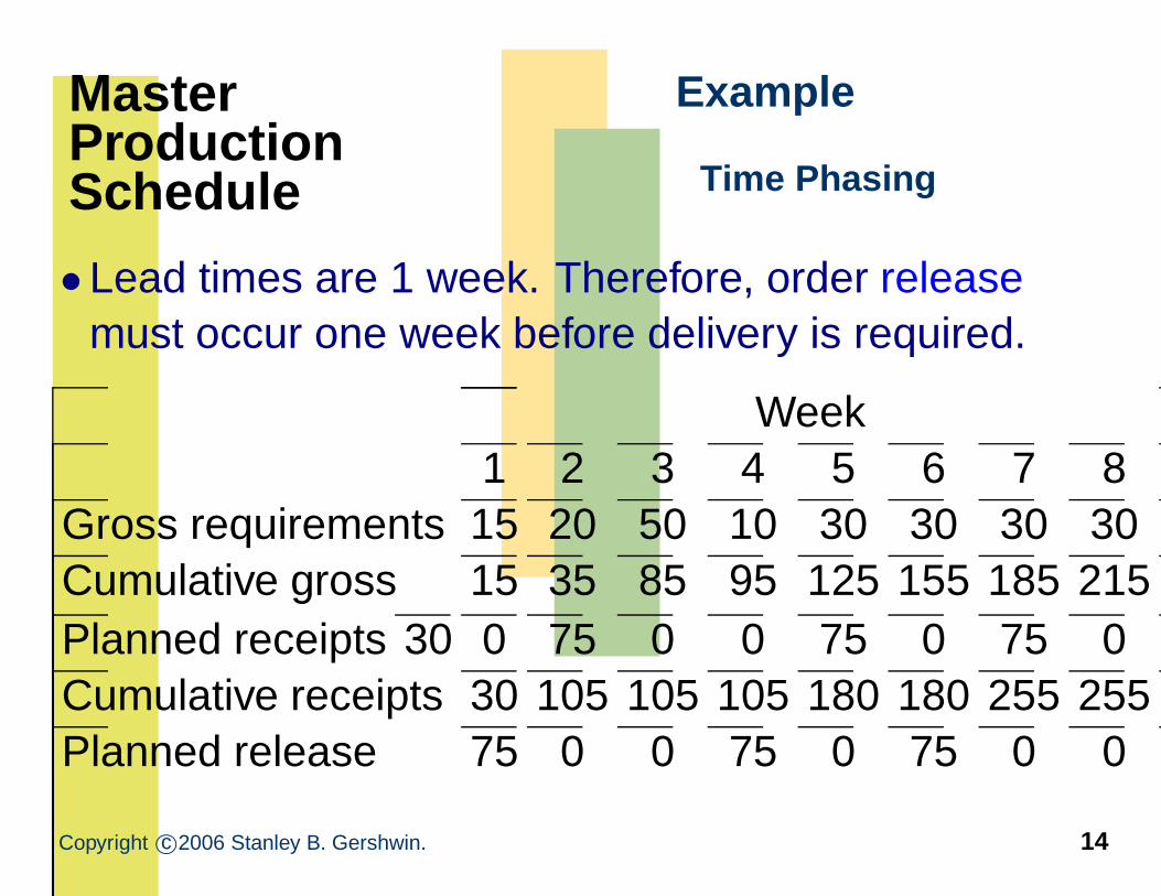
MasterProductionSchedule
Example
Time Phasing
• Lead times are 1 week. Therefore, order releasemust occur one week before delivery is required.
Week1 2 3 4 5 6 7 8
Gross requirements 15 20 50 10 30 30 30 30Cumulative gross 15 35 85 95 125 155 185 215Planned receipts 30 0 75 0 0 75 0 75 0Cumulative receipts 30 105 105 105 180 180 255 255Planned release 75 0 0 75 0 75 0 0
Copyright c©2006 Stanley B. Gershwin. 14
MasterProductionSchedule
Example
BOM Explosion
•Now, do exactly the same thing for all thecomponents required to produce the finished goods(level 1).
•Do it again for all the components of thosecomponents (level 2).
•Et cetera.
Copyright c©2006 Stanley B. Gershwin. 15
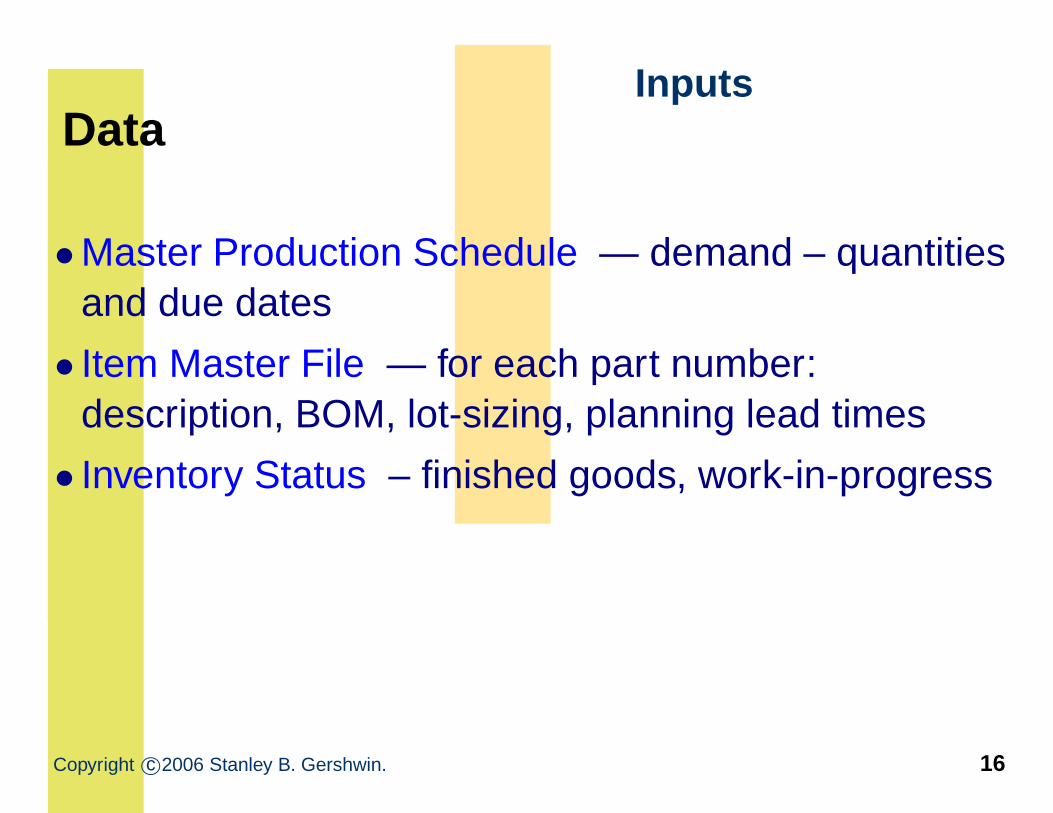
DataInputs
•Master Production Schedule — demand – quantitiesand due dates
• Item Master File — for each part number:description, BOM, lot-sizing, planning lead times
• Inventory Status – finished goods, work-in-progress
Copyright c©2006 Stanley B. Gershwin. 16
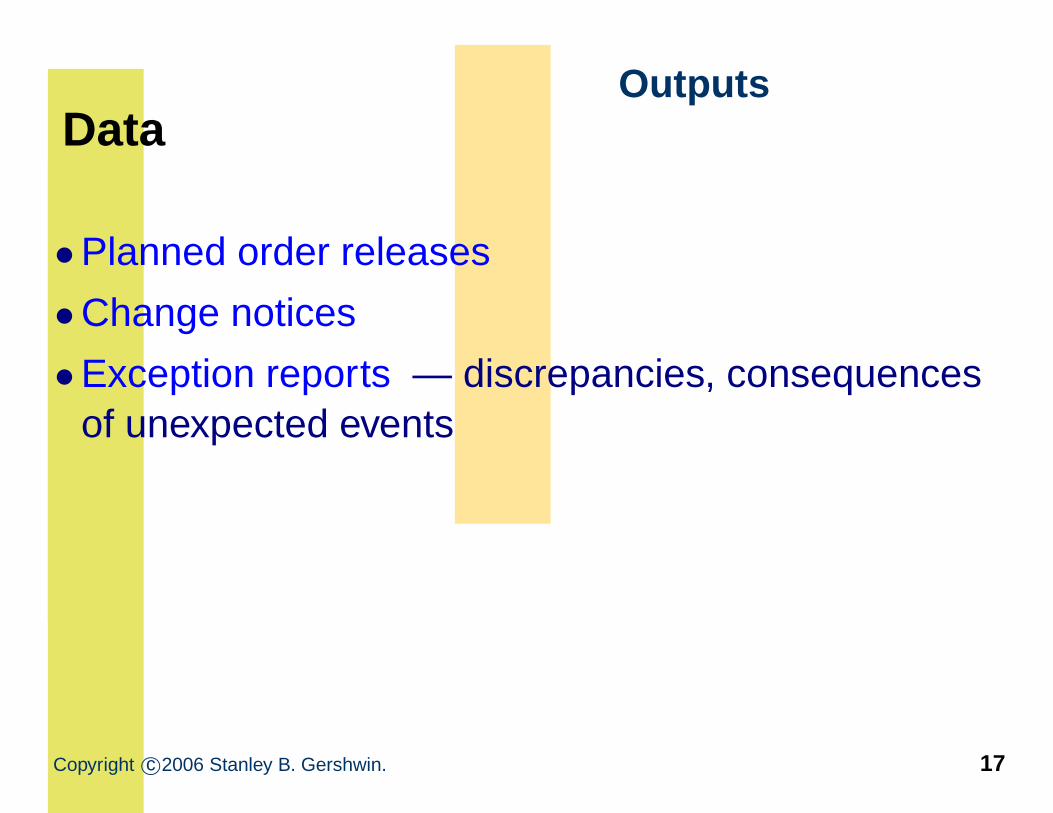
DataOutputs
•Planned order releases
•Change notices
•Exception reports — discrepancies, consequencesof unexpected events
Copyright c©2006 Stanley B. Gershwin. 17
MasterProductionSchedule
Definitions
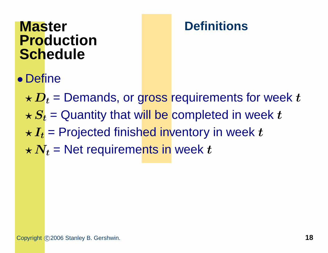
•Define
⋆Dt = Demands, or gross requirements for week t
⋆St = Quantity that will be completed in week t
⋆ It = Projected finished inventory in week t
⋆Nt = Net requirements in week t
Copyright c©2006 Stanley B. Gershwin. 18
MasterProductionSchedule
Netting
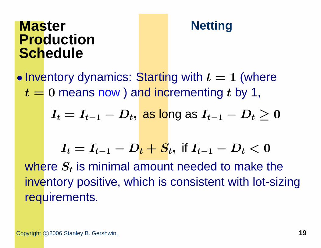
• Inventory dynamics: Starting with t = 1 (wheret = 0 means now ) and incrementing t by 1,
It = It−1 − Dt, as long as It−1 − Dt ≥ 0
It = It−1 − Dt + St, if It−1 − Dt < 0
where St is minimal amount needed to make theinventory positive, which is consistent with lot-sizingrequirements.
Copyright c©2006 Stanley B. Gershwin. 19
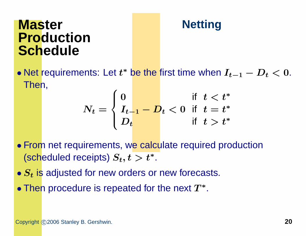
MasterProductionSchedule
Netting
• Net requirements: Let t∗ be the first time when It−1 − Dt < 0.Then,
0 if t < t∗
Nt =
It−1 − Dt < 0 if t = t∗
Dt if t > t∗
• From net requirements, we calculate required production(scheduled receipts) St, t > t∗.
•St is adjusted for new orders or new forecasts.
• Then procedure is repeated for the next T ∗.
Copyright c©2006 Stanley B. Gershwin. 20
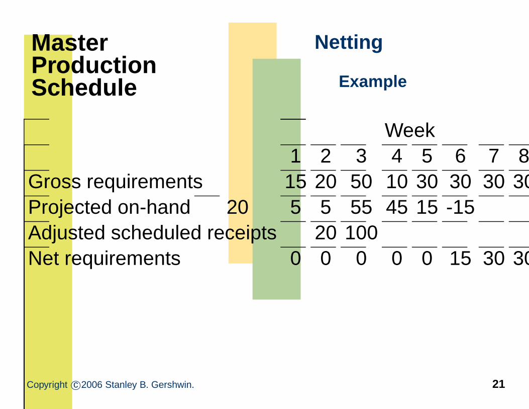
MasterProductionSchedule
Netting
Example
Week1 2 3 4 5 6 7 8
Gross requirements 15 20 50 10 30 30 30 30Projected on-hand 20 5 5 55 45 15 -15Adjusted scheduled receipts 20 100Net requirements 0 0 0 0 0 15 30 30
Copyright c©2006 Stanley B. Gershwin. 21
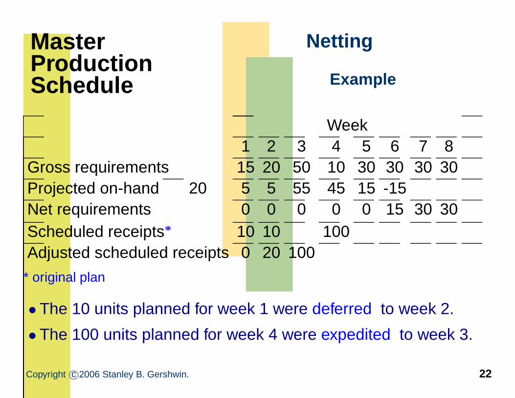
MasterProductionSchedule
Netting
Example
Week1 2 3 4 5 6 7 8
Gross requirements 15 20 50 10 30 30 30 30Projected on-hand 20 5 5 55 45 15 -15Net requirements 0 0 0 0 0 15 30 30Scheduled receipts∗ 10 10 100Adjusted scheduled receipts 0 20 100
* original plan
• The 10 units planned for week 1 were deferred to week 2.
• The 100 units planned for week 4 were expedited to week 3.
Copyright c©2006 Stanley B. Gershwin. 22
MasterProductionSchedule
Lot Sizing
Possible rules:
• Lot-for-lot: produce in a period the net requirementsfor that period. Maximum setups.
•Fixed order period: produce in a period the netrequirements for P periods.
•Fixed order quantity: always produce the samequantity, whenever anything is produced. EOQformula can be used to determine lot size.
Which satisfy the Wagner-Whitin property?
Copyright c©2006 Stanley B. Gershwin. 23
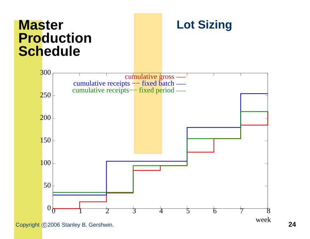
MasterProductionSchedule
Lot Sizing
cumulative gross 300
cumulative receipts −− fixed batchcumulative receipts−− fixed period
250
200
150
100
50
0 0 1 2 3 4 5 6 7 8week
Copyright c©2006 Stanley B. Gershwin. 24
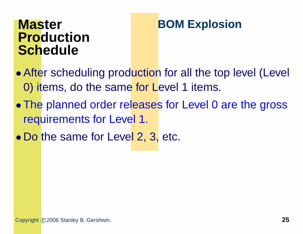
MasterProductionSchedule
BOM Explosion
•After scheduling production for all the top level (Level0) items, do the same for Level 1 items.
•The planned order releases for Level 0 are the grossrequirements for Level 1.
•Do the same for Level 2, 3, etc.
Copyright c©2006 Stanley B. Gershwin. 25
RealityUncertainty/Variability
•MRP is deterministic but reality is not. Therefore, thesystem needs safety stock and safety lead times .
•Safety stock protects against quantity uncertainties.
⋆You don’t know how much you will make, so plan tomake a little extra.
•Safety lead time protects against timinguncertainties.
⋆You don’t know exactly when you will make it, soplan to make it a little early.
Copyright c©2006 Stanley B. Gershwin. 26
RealityUncertainty/Variability
Safety Stock
• Instead of having a minimal planned inventory ofzero, the (positive) safety stock is the plannedminimal inventory level.
•Whenever the actual minimal inventory differs fromthe safety stock, adjust planned order releasesaccordingly.
Copyright c©2006 Stanley B. Gershwin. 27
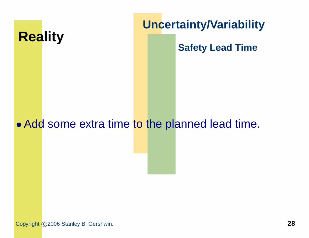
RealityUncertainty/Variability
Safety Lead Time
•Add some extra time to the planned lead time.
Copyright c©2006 Stanley B. Gershwin. 28
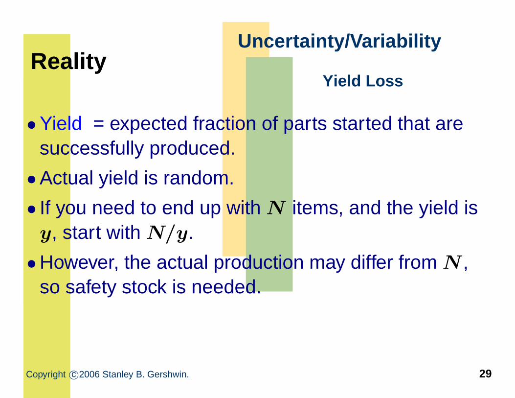
RealityUncertainty/Variability
Yield Loss
•Yield = expected fraction of parts started that aresuccessfully produced.
•Actual yield is random.
• If you need to end up with N items, and the yield isy, start with N/y.
•However, the actual production may differ from N ,so safety stock is needed.
Copyright c©2006 Stanley B. Gershwin. 29
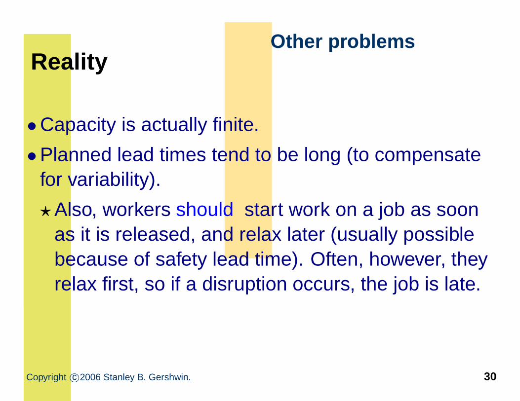
RealityOther problems
•Capacity is actually finite.
•Planned lead times tend to be long (to compensatefor variability).
⋆Also, workers should start work on a job as soonas it is released, and relax later (usually possiblebecause of safety lead time). Often, however, theyrelax first, so if a disruption occurs, the job is late.
Copyright c©2006 Stanley B. Gershwin. 30
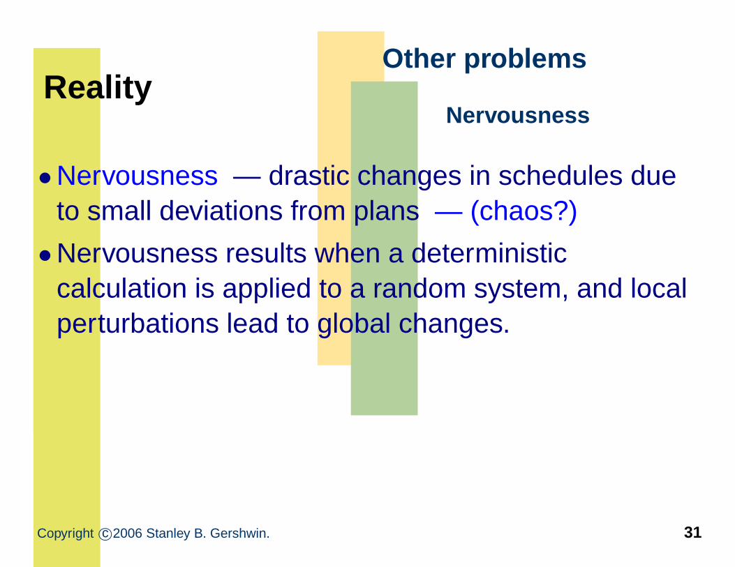
RealityOther problems
Nervousness
•Nervousness — drastic changes in schedules dueto small deviations from plans — (chaos?)
•Nervousness results when a deterministiccalculation is applied to a random system, and localperturbations lead to global changes.
Copyright c©2006 Stanley B. Gershwin. 31
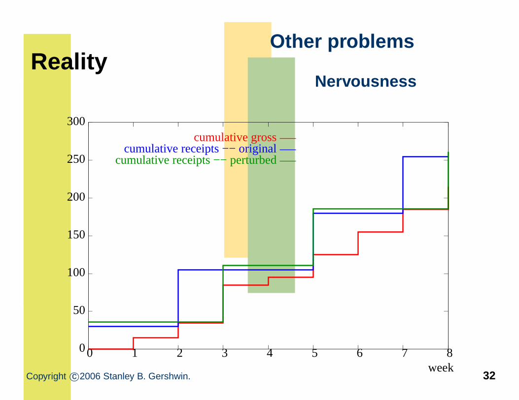
RealityOther problems
Nervousness
cumulative gross
cumulative receipts −− perturbedcumulative receipts −− original
300
250
200
150
100
50
0 0 1 2 3 4 5 6 7 8week
Copyright c©2006 Stanley B. Gershwin. 32
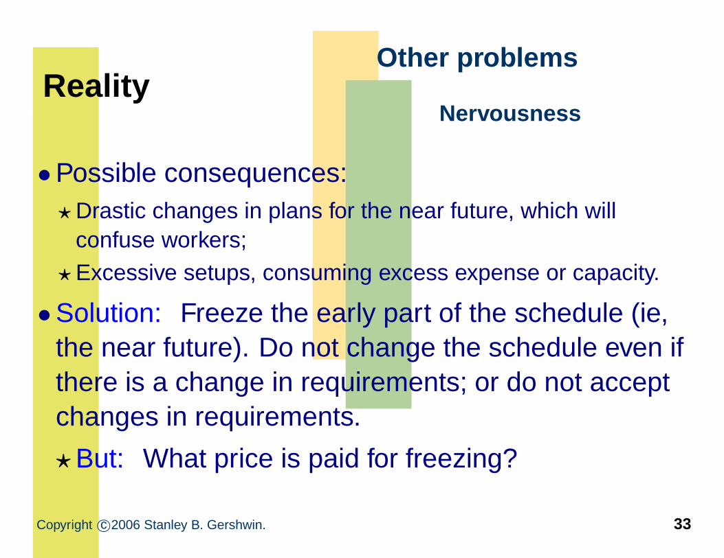
RealityOther problems
Nervousness
•Possible consequences:⋆ Drastic changes in plans for the near future, which will
confuse workers;
⋆ Excessive setups, consuming excess expense or capacity.
•Solution: Freeze the early part of the schedule (ie,the near future). Do not change the schedule even ifthere is a change in requirements; or do not acceptchanges in requirements.
⋆But: What price is paid for freezing?
Copyright c©2006 Stanley B. Gershwin. 33
RealityFundamental problem
•MRP is a solution to a problem whose formulation isbased on an unrealistic model, one which is⋆ deterministic⋆ infinite capacity
•As a result,⋆ it frequently produces non-optimal or infeasible schedules,
and⋆ it requires constant manual intervention to compensate for
poor schedules.
•On top of that, nervousness amplifies inevitablevariability.
Copyright c©2006 Stanley B. Gershwin. 34
MRP II
•Manufacturing Resources Planning⋆ MRP, and correction of some its problems,⋆ demand management,⋆ forecasting,⋆ capacity planning,⋆ master production scheduling,⋆ rough-cut capacity planning,⋆ capacity requirements planning (CRP),⋆ dispatching,⋆ input-output control.
Copyright c©2006 Stanley B. Gershwin. 35
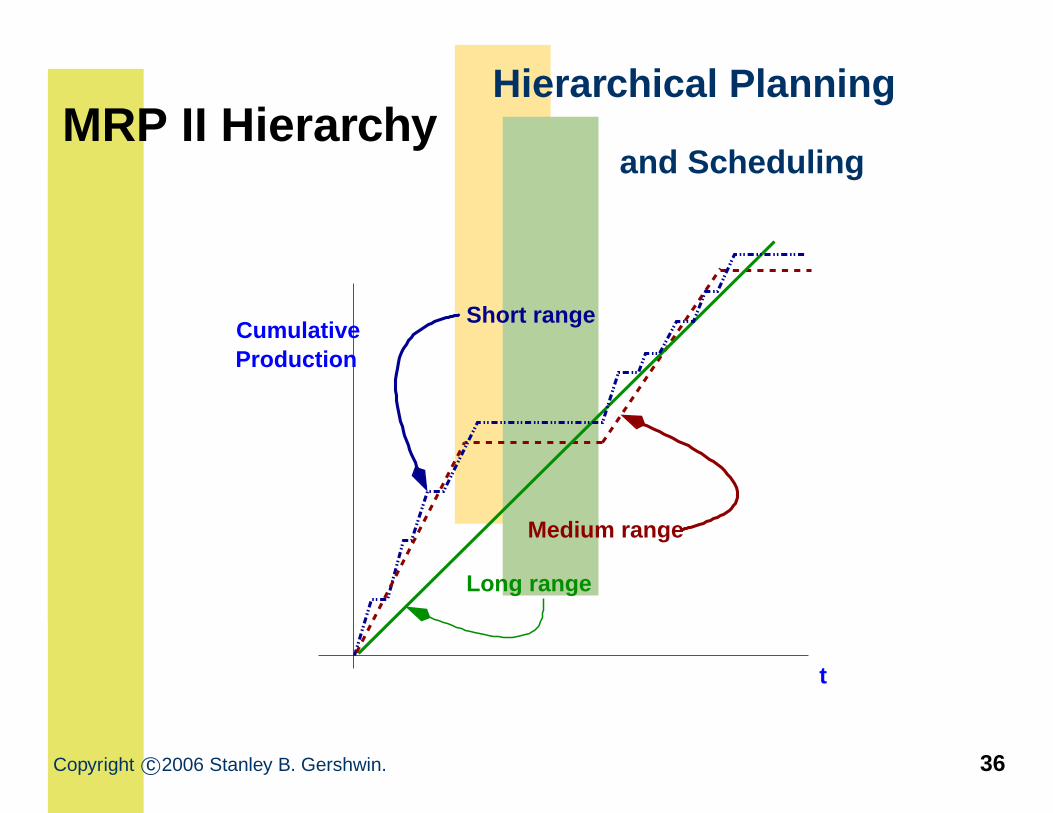
MRP II HierarchyHierarchical Planning
and Scheduling
CumulativeProduction
Long range
t
Medium range
Short range
Copyright c©2006 Stanley B. Gershwin. 36
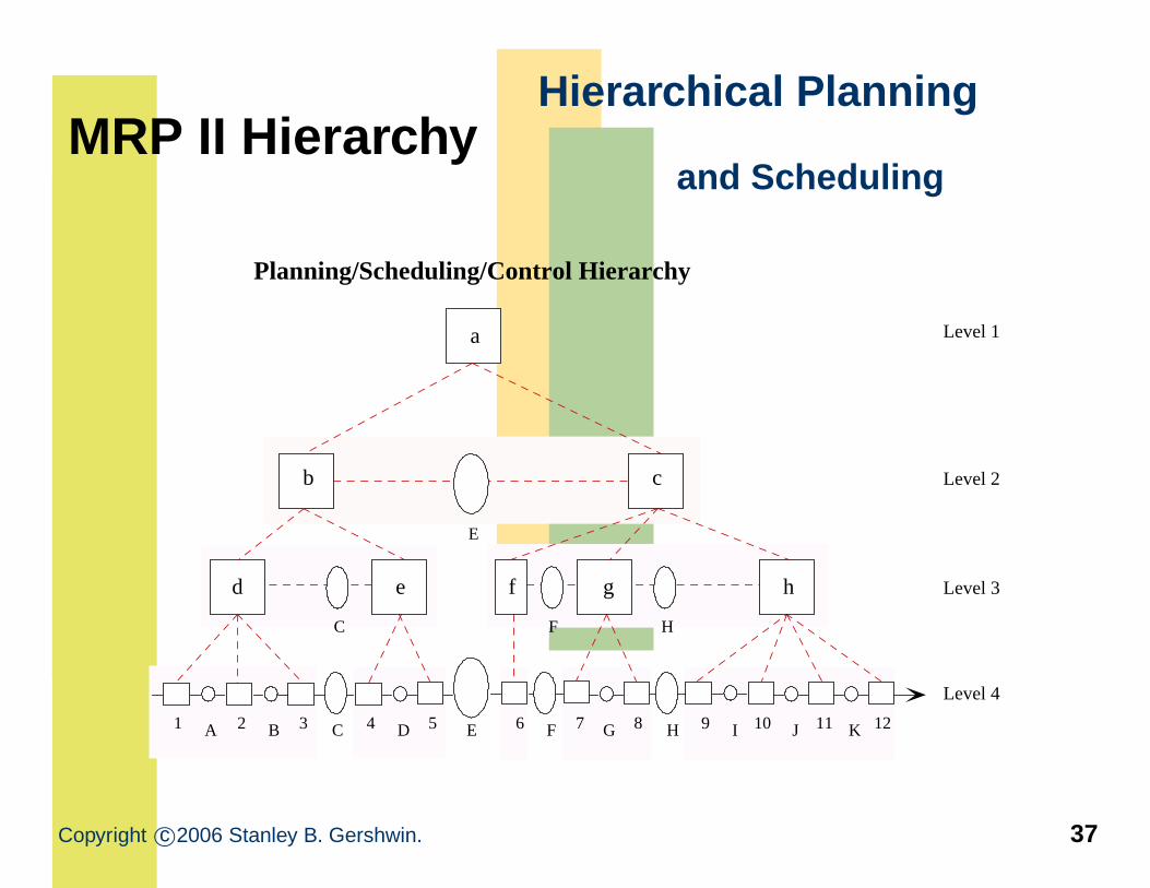
MRP II HierarchyHierarchical Planning
and Scheduling
F G H I J KA B C D E 6 7 8 9 10 11 121 2 3 4 5
C F H
E
Planning/Scheduling/Control Hierarchy
Level 1
Level 2
Level 3
Level 4
a
b c
d e f g h
Copyright c©2006 Stanley B. Gershwin. 37
MRP II HierarchyHierarchical Planning
General ideas
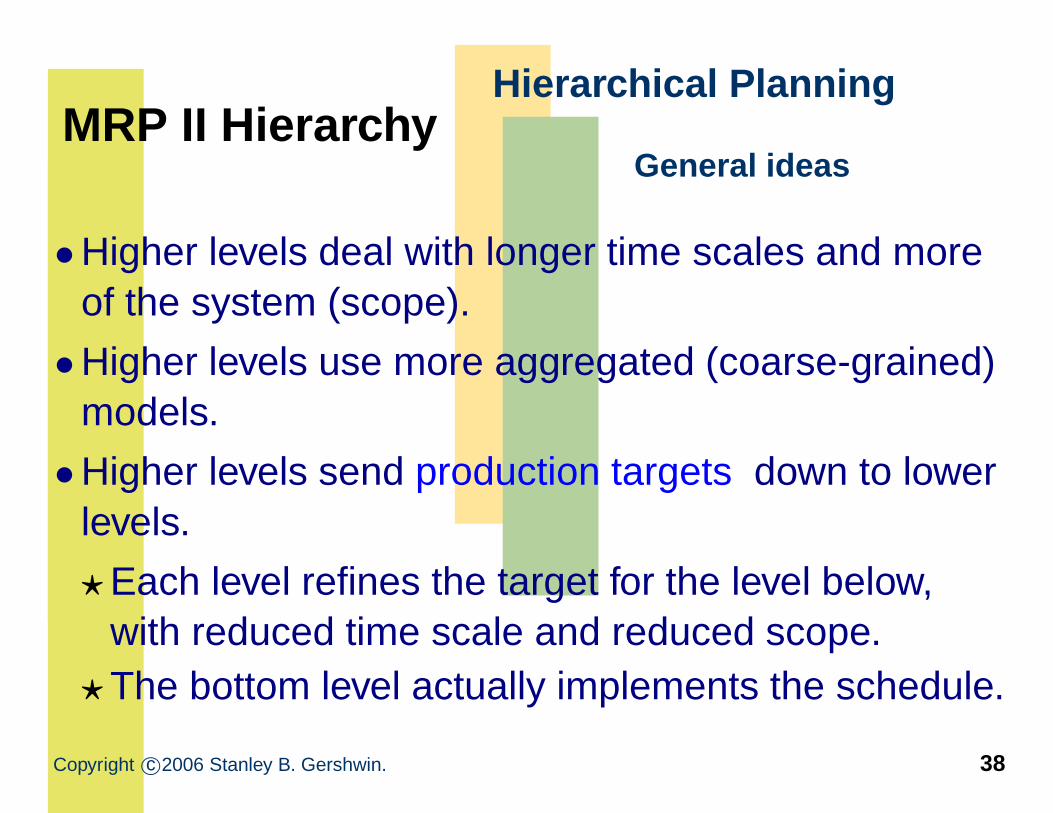
•Higher levels deal with longer time scales and moreof the system (scope).
•Higher levels use more aggregated (coarse-grained)models.
•Higher levels send production targets down to lowerlevels.
⋆Each level refines the target for the level below,with reduced time scale and reduced scope.
⋆The bottom level actually implements the schedule.
Copyright c©2006 Stanley B. Gershwin. 38
MRP II HierarchyHierarchical Planning
General ideas
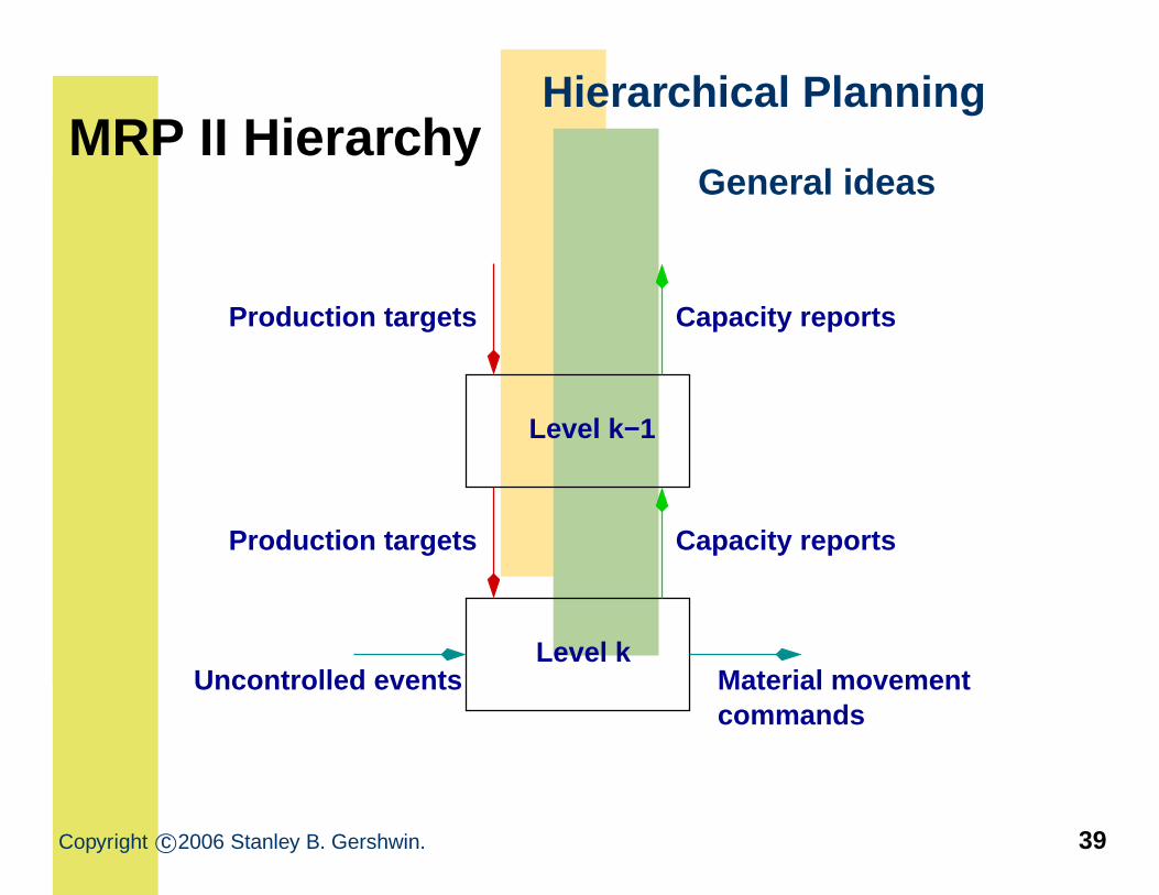
Production targets Capacity reports
Level k−1
Production targets Capacity reports
Level kUncontrolled events Material movement
commands
Copyright c©2006 Stanley B. Gershwin. 39
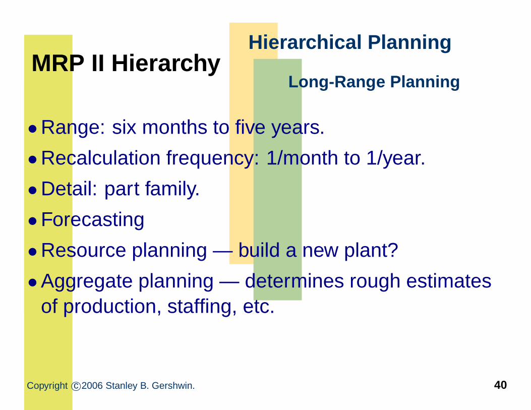
MRP II HierarchyHierarchical Planning
Long-Range Planning
•Range: six months to five years.
•Recalculation frequency: 1/month to 1/year.
•Detail: part family.
•Forecasting
•Resource planning — build a new plant?
•Aggregate planning — determines rough estimatesof production, staffing, etc.
Copyright c©2006 Stanley B. Gershwin. 40
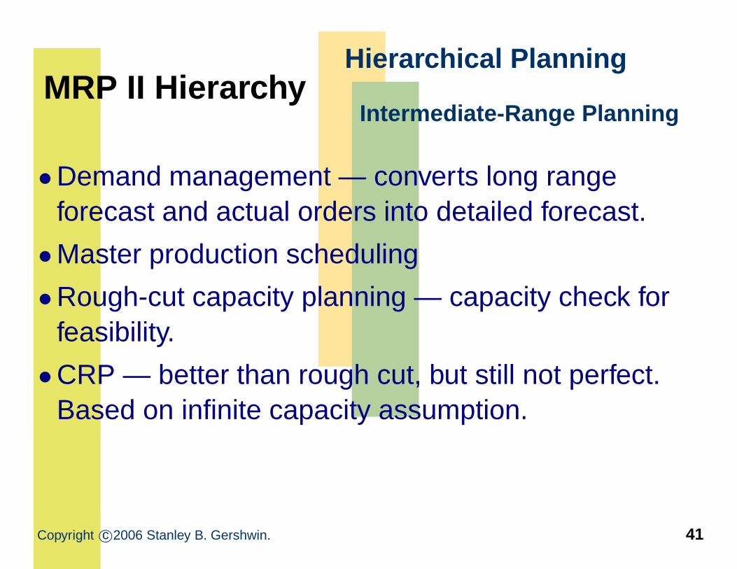
MRP II HierarchyHierarchical Planning
Intermediate-Range Planning
•Demand management — converts long rangeforecast and actual orders into detailed forecast.
•Master production scheduling
•Rough-cut capacity planning — capacity check forfeasibility.
•CRP — better than rough cut, but still not perfect.Based on infinite capacity assumption.
Copyright c©2006 Stanley B. Gershwin. 41
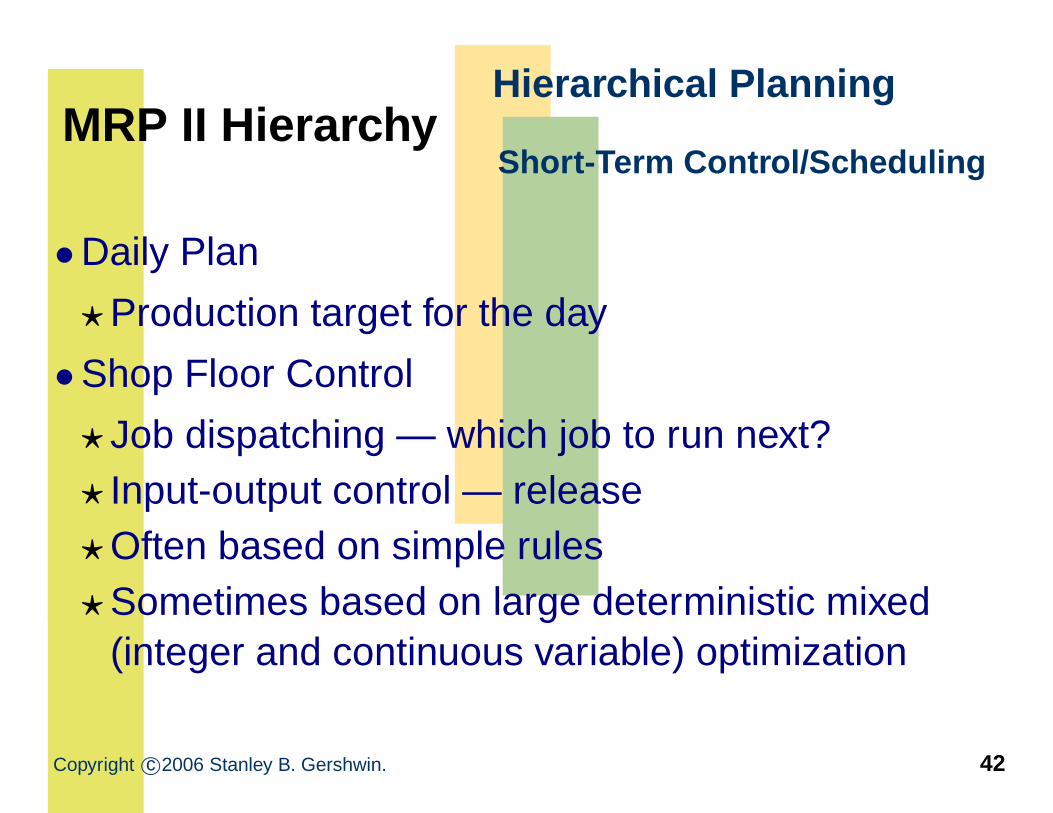
MRP II HierarchyHierarchical Planning
Short-Term Control/Scheduling
•Daily Plan
⋆Production target for the day
•Shop Floor Control
⋆ Job dispatching — which job to run next?⋆ Input-output control — release⋆Often based on simple rules⋆Sometimes based on large deterministic mixed
(integer and continuous variable) optimization
Copyright c©2006 Stanley B. Gershwin. 42
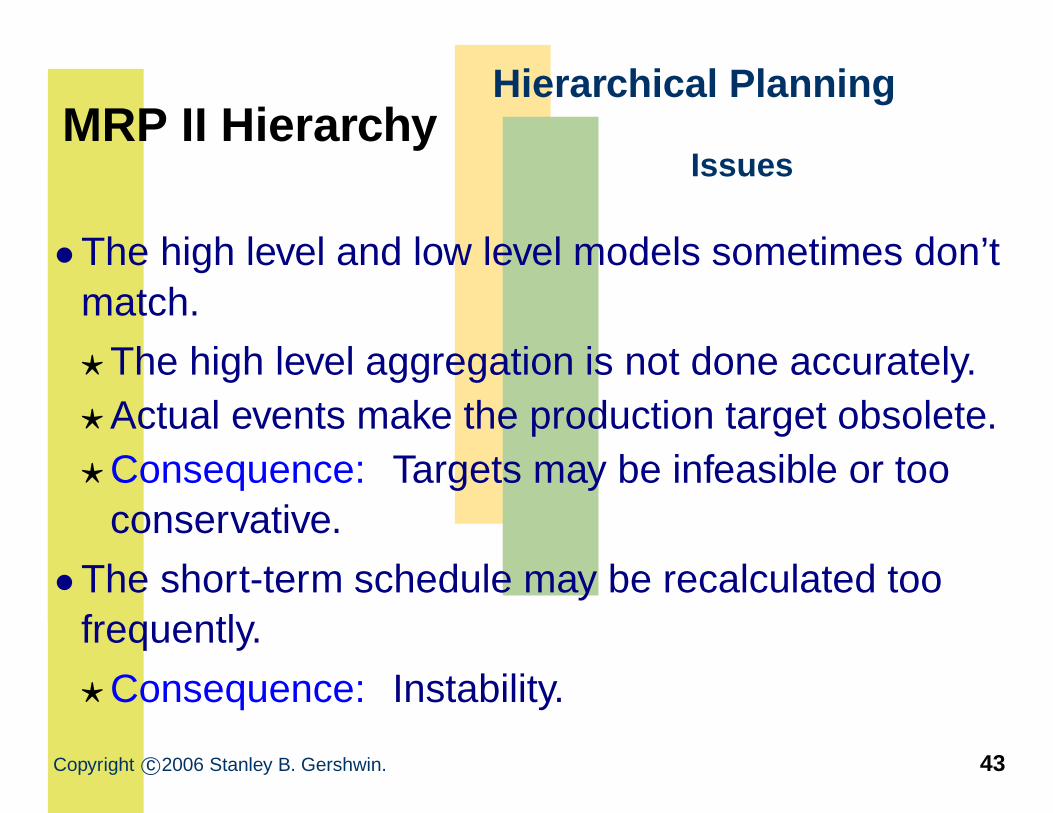
MRP II HierarchyHierarchical Planning
Issues
•The high level and low level models sometimes don’tmatch.
⋆The high level aggregation is not done accurately.⋆Actual events make the production target obsolete.⋆Consequence: Targets may be infeasible or too
conservative.
•The short-term schedule may be recalculated toofrequently.
⋆Consequence: Instability.
Copyright c©2006 Stanley B. Gershwin. 43

MIT OpenCourseWarehttps://ocw.mit.edu
2.854 / 2.853 Introduction To Manufacturing SystemsFall 2016
For information about citing these materials or our Terms of Use, visit: https://ocw.mit.edu/terms.


![SC L Series Catalog 2014 vf - clifrance.comclifrance.com/PDF/Hypertac/Lnew.pdf · 11 2.638 [67.00] LPa11 LEa11 12 2.854 [72.50] LPa12 LEa12 13 3.070 [78.00] LPa13 LEa13 14 3.287 [83.50](https://img.pdfslide.net/doc/110x75/6055d434c209144213179b80/sc-l-series-catalog-2014-vf-11-2638-6700-lpa11-lea11-12-2854-7250-lpa12.jpg)


![PERFORMANCE ENGINEERINGkohler-motors.ru/sites/kohler-motors.ru/files/... · thread r.h. sae 5/8" threaded shaft 21 4 per foot tapered shaft sae 72.50[2.854] 19 . 177 [. 755] 52.50[2.067]](https://img.pdfslide.net/doc/110x75/5fe045e149ced86d8b4bbbd6/performance-engineeringkohler-thread-rh-sae-58-threaded-shaft-21-4-per.jpg)