Embed Size (px)
Citation preview

Mitigating Hard Capacity Constraints in Facility Location Modeling
by
Kayse Maass
A dissertation submitted in partial fulfillment
of the requirements for the degree of
Doctor of Philosophy
(Industrial and Operations Engineering)
in The University of Michigan
2017
Doctoral Committee:
Professor Mark S. Daskin, Chair
Professor Hyun-Soo Ahn
Professor Xiuli Chao
Assistant Professor Siqian May Shen

ii
ACKNOWLEDGEMENTS
I am immensely grateful for the support and guidance I received from many people while
undertaking this Ph.D. First and foremost, I would like to thank my advisor, Dr. Mark S. Daskin,
for his continuous support and encouragement during my time at the University of Michigan.
Not only did he teach me how to become a better researcher, teacher, and mentor, Mark also
taught me how to become a better individual. I am especially grateful for the ways in which he
challenged me to see things from a variety of perspectives, provided space for me to voice my
ideas and concerns in a way that built my confidence, and shared his infectious love of puns. It is
my honor to have had the opportunity to work with and learn from him.
I would also like to thank the other members of my dissertation committee: Dr. Hyun-
Soo Ahn, Dr. Xiuli Chao, and Dr. Siqian Shen, for their insightful comments and suggestions of
my work over the past few years. To the many other collaborators, faculty, staff, and graduate
students at the University of Michigan who have enriched my life with your presence, thank you
for your encouragement, laughter, and friendship.
I gratefully acknowledge the financial support from the National Science Foundation
Graduate Research Fellowship Program, Rackham Merit Fellowship Program, and Department
of Industrial and Operations Engineering at the University of Michigan during my tenure as a
doctoral student. This support enabled me to conduct the independent research within this
dissertation and disseminate my findings worldwide. I am also immensely appreciative of the
time and effort Eve Gendron dedicated to help run some of the computational studies presented
in this dissertation.

iii
In addition to the mentors I have gained during my doctoral studies, many thanks are due
to my predoctoral mentors who have constantly served as a source of encouragement: my second
grade teacher, Mrs. Carol Wright (for finding creative ways to challenge me intellectually); my
high school calculus teacher and Math League coach, Mr. Reid Froiland (for affirming my high
school self in pursuing a career in STEM); my Bethel University community of support
including, Prof. Patrice Conrath (for her constant eternal perspective and for showing me how
operations research can help improve our world), Dr. Eric Gossett (for honing my attention to
detail and for creating an environment that fostered my self-confidence), Dr. William Kinney
(for encouraging me to pursue graduate school), and Drs. Paula and Steve Soneral (for their
continued insight into how to pursue your dreams while maintaining a work-life balance).
I would not be who I am today without the love and support of my family. My deepest
gratitude goes to my parents, Mark and Sue Lee, for always believing in me and encouraging me
to be myself. I am certain that the way they integrated math and problem-solving into our daily
life cultivated my love for analytic and inquisitive thought from a young age. I am also grateful
for the constant encouragement from Randy and Kathy Maass, and especially appreciate of
Kathy for introducing me to the field in which I am receiving my doctoral degree. Most of all, I
would like to thank my loving, encouraging, and patient husband, Zac, who faithfully supports
my dreams in more ways than I could have ever imagined.

iv
TABLE OF CONTENTS
ACKNOWLEDGEMENTS ......................................................................................................... ii
LIST OF FIGURES ..................................................................................................................... xi
LIST OF APPENDICES ........................................................................................................... xiv
LIST OF ABBREVIATIONS .................................................................................................... xv
LIST OF SYMBOLS ................................................................................................................. xvi
ABSTRACT ............................................................................................................................... xxx
CHAPTER 1: Introduction .......................................................................................................... 1
1.1 The Necessity of Mitigating Hard Capacity Constraints ................................................. 2
1.2 Research Contributions .................................................................................................... 4
1.3 Outline ............................................................................................................................ 10
CHAPTER 2: Literature Review .............................................................................................. 11
2.1 Taxonomy of Location Models ...................................................................................... 11
2.2 The Evolution of Capacitated Location Models ............................................................ 13
2.3 Methods of Mitigating Hard Capacity Constraints ........................................................ 17
2.3.1 Long-Term Capacity Flexibility ............................................................................... 17
2.3.2 Penalizing Excess Demand ....................................................................................... 18
2.3.3 Backlogged Demand ................................................................................................. 20
2.4 Daily Demands and Cyclic Allocations ......................................................................... 21

v
2.5 Chapter Summary ........................................................................................................... 26
CHAPTER 3: Inventory Modulated Capacitated Location Problem .................................... 27
3.1 Motivation ...................................................................................................................... 27
3.2 Model Formulation ......................................................................................................... 27
3.3 Model Properties ............................................................................................................ 32
3.3.1 NP-Hardness ............................................................................................................. 33
3.3.2 Benefits of the IMCLP .............................................................................................. 34
3.3.3 Theoretical Maximum Number of Multi-Soured Demand Nodes ............................ 41
3.4 Computational Results ................................................................................................... 45
3.4.1 Empirical Number of Multi-Sourced Demand Nodes .............................................. 49
3.4.2 Comparison to CFLP ................................................................................................ 51
3.4.3 Effect of Problem Size .............................................................................................. 54
3.5 Chapter Summary ........................................................................................................... 59
CHAPTER 4: A Cyclic Allocation Model for the IMCLP ...................................................... 62
4.1 Motivation ...................................................................................................................... 62
4.2 Model Formulation ......................................................................................................... 63
4.3 Model Properties ............................................................................................................ 66
4.4 Additional Constraints .................................................................................................... 68
4.4.1 Restricting the Number of Different Allocations...................................................... 69
4.4.2 Weekday and Weekend Allocations ......................................................................... 70
4.4.3 Restricting the Maximum Allowed Travel Time ...................................................... 72
4.5 Computational Results ................................................................................................... 75
4.5.1 Restricting the Number of Different Allocations...................................................... 77

vi
4.5.2 Restricting the Maximum Allowed Travel Time ...................................................... 80
4.5.3 Allocation Composition ............................................................................................ 87
4.5.4 Solution Robustness .................................................................................................. 90
4.6 Chapter Summary ........................................................................................................... 92
CHAPTER 5: Chance Constrained IMCLP with Uncertain Demand .................................. 94
5.1 Motivation ...................................................................................................................... 94
5.2 Joint Chance Constrained Formulation .......................................................................... 95
5.2.1 Single Stage Formulation with Probabilistic Constraint ........................................... 97
5.2.2 MIP Reformulation ................................................................................................... 99
5.3 Solution Methods ......................................................................................................... 101
5.3.1 Two-Stage Benders Decomposition Approach ....................................................... 101
5.3.2 Three-Stage Decomposition Approach ................................................................... 110
5.3.3 Proof of the Validity of Feasibility Cuts (5.65) ...................................................... 117
5.3.4 Relaxed Joint Chance Constraint ............................................................................ 119
5.4 Additional Chance Constraints ..................................................................................... 122
5.4.1 Two Stage Decomposition ...................................................................................... 124
5.4.2 Three Stage Decomposition .................................................................................... 124
5.5 Computational Results ................................................................................................. 131
5.5.1 Determining the Appropriate Number of Scenarios ............................................... 132
5.5.2 Comparison of Solution Times ............................................................................... 140
5.5.3 Optimal Facility Locations ..................................................................................... 142
5.5.4 Effect of Using Individual or Hybrid Chance Constraints ...................................... 148
5.5.5 Comparison to IMCLP Solution ............................................................................. 152

vii
5.6 Chapter Summary ......................................................................................................... 157
CHAPTER 6: Extensions and Conclusions ............................................................................ 159
6.1 Introduction .................................................................................................................. 159
6.2 Queueing Model to Approximate Average Backlog .................................................... 159
6.2.1 Queueing Formulation ............................................................................................ 160
6.2.2 Approximation Formulas for 𝔼[ ]jV ...................................................................... 161
6.2.3 Model Summary and Challenges ............................................................................ 163
6.3 Incremental Backlog Cost Model ................................................................................. 164
6.3.1 Linear Programming Model Formulation ............................................................... 164
6.3.2 Determining the Incremental Cost Values .............................................................. 165
6.3.3 Model Summary and Challenges ............................................................................ 167
6.4 Outbound Shipment Model .......................................................................................... 168
6.5 Additional Methods of Incorporating Capacity Flexibility .......................................... 172
6.5.1 Endogenous Capacity Flexibility ............................................................................ 172
6.5.2 Exogenous Capacity Fluctuations ........................................................................... 175
6.6 Conclusions and Contributions .................................................................................... 177
APPENDICES ........................................................................................................................... 182
BIBLIOGRAPHY ..................................................................................................................... 190

viii
LIST OF TABLES
Table 1: Example demand ............................................................................................................ 35
Table 2: Example travel time (in days) ......................................................................................... 35
Table 3: Daily demand received: optimal IMCLP solution .......................................................... 38
Table 4: Daily demand received: optimal CFLP assignments in IMCLP model ......................... 38
Table 5: Cost comparison ............................................................................................................. 38
Table 6: Cost of optimal data-driven CFLP solution .................................................................... 40
Table 7: Daily demand received: optimal data-driven CFLP ....................................................... 41
Table 8: Multi-sourced example: daily demand generated ........................................................... 43
Table 9: Multi-sourced example 2 solution: demand allocation ................................................... 43
Table 10: Multi-sourced example 2 solution: total demand arriving at processing facility ......... 44
Table 11: Demand statistics for 5 largest demand sites ................................................................ 46
Table 12: Population Range of 500 Largest US Counties ............................................................ 46
Table 13: Daily processing capacity per candidate facility .......................................................... 48
Table 14: Number of multi-sourced demand sites; 𝑎 = 1, 𝑏 = 3 ................................................ 50
Table 15: Solution times (in seconds) or % optimality gap (indicated by shading) within 1 hour
using a generic solver; 𝑎 = 1, 𝑏 = 3 ........................................................................... 55
Table 16: Example mean demand rate pattern .............................................................................. 67
Table 17: Optimal cyclic assignments when 60b — example instance .................................... 67
Table 18: Effect of varying the value of 𝓃 ................................................................................... 78
Table 19: Effect of varying the value of 𝓃: computational results; 𝑎 = 2, 𝑏 = 20 ..................... 79

ix
Table 20: Effect of restricting travel time; 𝑎 = 2, 𝑏 = 20 ........................................................... 81
Table 21: Cyclic allocations for Salt Lake, UT ............................................................................ 85
Table 22: Effect of restricting the time difference; 𝑎 = 2, 𝑏 = 20 .............................................. 86
Table 23: Effect of imposing closest assignment constraints; 𝑎 = 2, 𝑏 = 20 ............................. 87
Table 24: % Increase in Cost from using the Optimal Locations and Allocations of Instance 1
instead of the Optimal Solution for the Particular Instance; 𝑎 = 2, 𝑏 = 20 ............... 91
Table 25: Comparison of the types of chance constraints .......................................................... 123
Table 26: Lower bound on the probability that the optimal MIP-JCC objective function value
obtained from a subset of |Ω′| demand scenarios with 𝜏′ = 0.1 is a lower bound on the
optimal JCC objective function value with 𝜏 ............................................................. 137
Table 27: The minimum MIP-JCC objective function value obtained from ℐ = 20 repetitions of
a subset of |Ω′| demand scenarios is a lower bound on the optimal objective function
value of JCC (with associated acceptable exceedance probability of 𝜏) with confidence
1 − 𝛿 .......................................................................................................................... 138
Table 28: Percent total cost increases from the case in which all demand sites are candidate
processing facilities; 𝑎 = 15, 𝑏 = 30; 𝜃 = 91, 𝜏′ = 0.1 ........................................... 145
Table 29: Percent decrease in solution time compared to the case in which all demand sites are
candidate processing facilities; 𝑎 = 15, 𝑏 = 30; 𝜃 = 91, 𝜏′ = 0.1 ........................... 145
Table 30: More facilities are located as the number of demand and candidate nodes increase,
which results in a decrease in capacity utilization; 𝑎 = 15, 𝑏 = 30 .......................... 147
Table 31: Optimal IMCLP and MIP-JCC cost and backlog comparison, 𝑎 = 5, 𝑏 = 10; ......... 155

x
Table 32: Performance of optimal IMCLP instance location and allocation decisions in MIP-JCC
when IMCLP solution enforces daily facility backlog limit of 𝜃 = 91; 𝑎 = 5, 𝑏 = 10
.................................................................................................................................... 156
Table 33: Detailed performance of optimal location and allocation decisions for IMCLP
instances two and four in MIP-JCC when IMCLP solution enforces daily facility
backlog limit of 𝜃 = 91; 𝑎 = 5, 𝑏 = 10 ................................................................... 157
Table 34: Effect of population weight on location cost and optimal solution; Poisson distributed
demand; a=1, b=3 ....................................................................................................... 186

xi
LIST OF FIGURES
Figure 1: Taxonomy of Location Models ..................................................................................... 12
Figure 2: Optimal CFLP and IMCLP solutions for the example .................................................. 36
Figure 3: Effect of using the CFLP solution in the IMCLP; 𝑎 = 1 .............................................. 39
Figure 4: Effect of increasing backlog weight, 50 demand & candidate nodes, 100 days, 𝑎 = 1 50
Figure 5: Optimal CFLP Solution; 50 demand & candidate nodes, 𝑎 = 1; ................................. 52
Figure 6: Optimal IMCLP solution; 50 demand & candidate nodes, 𝑎 = 1, 𝑏 = 100; ................ 53
Figure 7: Effect of changing number of candidate nodes; 100 demand & candidate nodes, 100
days, 𝑎 = 1, 𝑏 = 3 ....................................................................................................... 56
Figure 8: IMCLP solution progress as size of candidate node set varies; 100 days; 𝑎 = 1, 𝑏 = 3
...................................................................................................................................... 57
Figure 9: CFLP solution progress as size of candidate node set varies; 𝑎 = 1 ............................ 58
Figure 10: Effect of increasing time horizon, 50 demand & candidate nodes, 𝑎 = 1, 𝑏 = 3 ....... 59
Figure 11: Total backlog—example instance ............................................................................... 68
Figure 12: Total cost—example instance ..................................................................................... 68
Figure 13: Average daily facility location costs for the cyclic allocation model, 𝑧 = 10,000,
𝑤 = 0.0001 .................................................................................................................. 77
Figure 14: Cost effect of restricting travel time; max 7,...,29t days; 𝑎 = 2, 𝑏 = 20 ............. 81
Figure 15: Cost effect of restricting travel time; 𝑎 = 2, 𝑏 = 20 .................................................. 82

xii
Figure 16: Optimal locations and allocations arriving on weekdays for Case 3; 𝑎 = 2, 𝑏 = 20,
max 11t ...................................................................................................................... 83
Figure 17: Optimal locations and allocations arriving on Saturdays for Case 3; 𝑎 = 2, 𝑏 = 20,
max 11t ...................................................................................................................... 83
Figure 18: Optimal locations and allocations arriving on Sundays for Case 3; 𝑎 = 2, 𝑏 = 20,
max 11t ...................................................................................................................... 84
Figure 19: Types of allocations in the optimal solution as the backlog cost varies; 𝑎 = 2 .......... 89
Figure 20: Types of allocations in the optimal solution as the backlog cost varies; 𝑎 = 2 .......... 89
Figure 21: % decrease in cost obtained by using the cyclic allocation model as compared to the
IMCLP model; 𝑎 = 2 ................................................................................................... 90
Figure 22: Variability in optimal objective function value as number of scenarios changes; 20
instances solved for each scenario size; Poisson distributed demand ........................ 134
Figure 23: Percent difference between the lower and upper bounds on two standard deviations
from the mean optimal objective function value; 20 instances solved for each scenario
size; Poisson distributed demand ............................................................................... 134
Figure 24: Variability in optimal objective function values as number of scenarios changes; 20
instances solved for each scenario size; Truncated Normal demand distribution ..... 135
Figure 25: Percent difference between the lower bound and upper bounds on two standard
deviations from the mean optimal objective function value; 20 instances solved for
each scenario size; Truncated Normal demand distribution ...................................... 136
Figure 26: Comparison of solution methods; 𝑎 = 15, 𝑏 = 30; 𝜃 = 91, 𝜏′ = 0.1 ...................... 141
Figure 27: Five most populous counties ..................................................................................... 142

xiii
Figure 28: Optimal facility locations for the instance with 50 demand & candidate nodes;
𝑎 = 15, 𝑏 = 30; 𝜃 = 91, 𝜏′ = 0.1 ............................................................................. 143
Figure 29: Optimal facility locations for the instance with 500 demand & candidate nodes;
𝑎 = 15, 𝑏 = 30; 𝜃 = 91, 𝜏′ = 0.1 ............................................................................. 143
Figure 30: Tradeoffs of reducing the candidate node set for the 500 demand node instance; the
number of candidate nodes used is in parenthesis; 𝑎 = 15, 𝑏 = 30; 𝜃 = 91, 𝜏′ = 0.1
.................................................................................................................................... 145
Figure 31: More facilities are located as the number of demand and candidate nodes increase. 148
Figure 32: The optimal solution has excess system-wide capacity due to locating extra facilities.
.................................................................................................................................... 148
Figure 33: Comparison of the optimal cost of the MIP-JCC, MIP-HCC, and MIP-ICC chance
constraints; Poisson distributed demand, 50 scenarios, 𝑎 = 5, 𝑏 = 10, 𝜃 = 91....... 150
Figure 34: Comparison of the optimal cost of the MIP-JCC, MIP-HCC, and MIP-ICC chance
constraints; Normally distributed demand, 10 scenarios, 𝑎 = 5, 𝑏 = 10, 𝜃 = 91 .... 150
Figure 35: Example scenario of backlogged demand at Fresno, CA; Normally distributed
demand, 10 scenarios, 𝑎 = 5, 𝑏 = 10; 𝜃 = 91, 𝜏′ = 0.2 .......................................... 152
Figure 36: Comparison of the optimal IMCLP and MIP-JCC location and allocation solutions;
Poisson distributed demand; 𝑎 = 5, 𝑏 = 10; For MIP-JCC: 𝜃 = 91, 𝜏′ = 0.1 ........ 154
Figure 37: Average backlog at a processing facility that results from the average amount of total
daily demand arriving at the facility; Poisson distributed arriving demands; 100jk
.................................................................................................................................... 167
Figure 38: The optimal facility locations listed in Table 34 ....................................................... 187

xiv
LIST OF APPENDICES
APPENDIX A: The Data-Driven CFLP ................................................................................. 183
APPENDIX B: Effect of Population Weight .......................................................................... 185
APPENDIX C: Proof of the Validity of Feasibility Cuts (5.89) ............................................ 188

xv
LIST OF ABBREVIATIONS
CFLP Capacitated Fixed Charge Location Problem
i.i.d. Independent and identically distributed
IMCLP Inventory Modulated Capacitated Location Problem
UFLP Uncapacitated Fixed Charge Location Problem

xvi
LIST OF SYMBOLS
Sets
𝐶 Set identifying the number of consecutive days to couple in the relaxed joint chance
constraint (5.74)
𝐷 Set of days; indexed by 𝑑
𝐷𝑝 ≔ 𝑑 ∈ 𝐷: 𝑑 𝑚𝑜𝑑 |𝑃| = 𝑝, 𝑑 > 𝑡∗ Set of days in 𝐷 corresponding to cycle day 𝑝 ∈ 𝑃 after
the warm-up period
ℱ ≔ (𝑿,𝒀): ∃𝑽,𝑾, 𝒁: (2.2) - (2.4), (3.6), (5.10) - (5.12), (5.15) - (5.19), and (5.22)
are satisfied
ℱ ≔ (𝑿, 𝒀): ∃𝑽,𝑾, 𝒁: (2.2) - (2.4), (3.6), (5.15) - (5.19), (5.22), and (5.80) - (5.82)
are satisfied
ℱ ≔ (𝑿, 𝒀): ∃𝑽,𝑾, 𝒁: (2.2) - (2.4), (3.6), (5.15) - (5.19), (5.22), and (5.83) - (5.85)
are satisfied
𝐼 Set of demand sites; indexed by 𝑖
𝐼𝑗𝜓
For a given, facility 𝑗 ∈ 𝐽 and 𝜓 ∈ Ψ, the set of demand sites allocated to 𝑗
𝐼𝜓
For a given, facility 𝑗 ∈ 𝐽 and 𝜓 ∈ Ψ𝑗, the set of demand sites allocated to 𝑗
𝐽 Set of candidate processing facility locations; indexed by 𝑗
𝐽𝜓 For a given 𝜓 ∈ Ψ, the set of located candidate facilities that violate the backlog
threshold 𝜃
𝑃 Set of cycle-days (e.g., days of the week); indexed by 𝑝

xvii
℘𝜔′𝑗 Feasible region of D-M1S2(𝜔′, 𝑗)
𝑄𝑖𝑗 Set of cycle days for which demand shipped from 𝑖 ∈ 𝐼 would arrive at facility 𝑗 ∈ 𝐽 on
the weekend
𝑅𝑖𝑗 Set of cycle days for which demand shipped from 𝑖 ∈ 𝐼 would arrive at facility 𝑗 ∈ 𝐽
during the weekday
𝒮𝜓 ≔ (𝑖, 𝑗) ∈ 𝐼 × 𝐽: 𝑌𝑖𝑗𝜓= 1 and ∃𝜔′ ∈ Ω′; 𝑑 ∈ 𝑡∗ + 1,… , |𝐷| + 1 with 𝑉𝑗𝑑
𝜔′𝜓> 𝜃
Φ𝜔′𝑗 Set of extreme points of ℘𝜔′𝑗; indexed by 𝜙
Φ𝜔′ Set of extreme points of (5.47) - (5.52) for scenario 𝜔′ ∈ Ω′; indexed by 𝜙
Φ =∪ω′∈Ω′ Φω′
Φ ⊆ Φ Set of optimality cuts generated; used in solution approach 1 for the joint chance
constrained problem
Φ Set of optimality cuts generated; used in solution approach 2 for the joint, hybrid, and
individual chance constrained problems
Ψ𝜔′𝑗 Set of extreme rays of ℘𝜔′𝑗; indexed by 𝜓
Ψ𝜔′ Set of extreme rays of (5.47) - (5.52) for scenario 𝜔′ ∈ Ω′; indexed by 𝜓
Ψ𝜔′ ⊆ Ψ𝜔′ Set of infeasibility cuts generated; used in solution approach 1 for the joint chance
constrained problem
Ψ Set of infeasibility cuts generated; used in solution approach 2 for the joint chance
constrained problem
Ψ𝑗 Set of infeasibility cuts generated for candidate facility 𝑗 ∈ 𝐽 ; used in solution approach 2
for the hybrid and individual chance constrained problems
Ω Set of all possible demand scenarios

xviii
Ω′ ⊆ Ω Subset of all possible demand scenarios; assumed finite
Ω Set of all possible capacity scenarios, assumed finite
(𝜸𝜔′𝑗𝜙, 𝝅𝜔
′𝑗𝜙, 𝜂𝜔′𝑗𝜙, 𝝁𝜔
′𝑗𝜙) ∈ Φω′𝑗
(𝜸𝜔′𝑗𝜓, 𝝅𝜔
′𝑗𝜓, 𝜂𝜔′𝑗𝜓, 𝝁𝜔
′𝑗𝜓) ∈ Ψ𝜔′𝑗
Parameters
𝑎 ≥ 0 Cost (in dollars) of transporting one item for one day
𝑏𝑗 ≥ 0 Cost (in dollars) of holding one item in backlog for one day at facility 𝑗 ∈ 𝐽
𝑏 ≥ 0 Cost (in dollars) of holding one item in backlog for one day; not facility specific
𝑗 ≥ 0 Daily cost of purchasing one additional unit of capacity at facility 𝑗 ∈ 𝐽
𝒷𝑗𝑙 The incremental backlog cost associated with assigning an average of 𝑙 demands to
facility 𝑗 ∈ 𝐽 each day rather than 𝑙 − 1 demands
𝑐𝑖𝑗 = 1
0
If 𝑡𝑖𝑗 ≤ 𝑡𝑚𝑎𝑥Otherwise
𝑑∗ Time horizon (in days; does not include warm-up period)
𝑗 Maximum number of days an item is allowed to be held in backlog at facility 𝑗 ∈ 𝐽
𝑓𝑗 Daily fixed cost of locating at facility 𝑗 ∈ 𝐽; in the cyclic-allocation model, the average
daily fixed location cost at 𝑗 ∈ 𝐽
ℎ𝑖 Average demand per unit of time generated at demand site 𝑖 ∈ 𝐼
ℎ𝑖𝑑 Demand that is generated at demand site 𝑖 ∈ 𝐼 on day 𝑑 ∈ 𝐷
ℎ𝑖𝑑 Random daily demand parameter generated at demand point 𝑖 ∈ 𝐼 on day 𝑑 ∈ 𝐷
ℎ𝑖𝑑𝜔 Realization of random demand ℎ𝑖𝑑 in scenario 𝜔 ∈ Ω, ∀𝑖 ∈ 𝐼, 𝑑 ∈ 𝐷
ℎ𝑖𝑑𝜔′ Realization of random demand ℎ𝑖𝑑 in scenario 𝜔′ ∈ Ω′, ∀𝑖 ∈ 𝐼, 𝑑 ∈ 𝐷

xix
ℐ Number of demand instances with a scenario size of |Ω′|; used to determine appropriate
number of scenarios to use in MIP-JCC; indexed by 𝒾
𝑘𝑗 Capacity of facility 𝑗 ∈ 𝐽 in items processed per day
𝑘𝑗𝑝 Capacity of facility 𝑗 ∈ 𝐽 in items processed per day on cycle day 𝑝 ∈ 𝑃
𝑘𝑗𝑚𝑎𝑥 ≥ 0 Maximum amount of additional capacity facility 𝑗 ∈ 𝐽 can purchase each day
𝑗 Increment size of extra daily capacity available for purchase at facility 𝑗 ∈ 𝐽
𝑘𝑗 Parameter such that 𝑘𝑗 − 𝑘𝑗 is the initial daily processing capacity of facility 𝑗 ∈ 𝐽 before
employees are trained
𝑘𝑗𝑟𝑎𝑡𝑒 Rate of capacity increase due to employee learning
𝑗𝑑 Random daily capacity at facility 𝑗 ∈ 𝐽 on day 𝑑 ∈ 𝑡∗ + 1,… , |𝐷|
𝑗𝑑 Realization of random capacity 𝑗𝑑 in scenario ∈ Ω at facility 𝑗 ∈ 𝐽 on day 𝑑 ∈ 𝐷
𝑚 Maximum travel day difference allowed between a demand site and its weekday facility
assignment, and the same demand site and its weekend facility assignment
𝑀1 Sufficiently large integer such that if 𝑉𝑗𝑑𝜔′ > 𝜃 for some facility 𝑗 ∈ 𝐽 on some day
𝑑 ∈ 𝑡∗ + 1,… , |𝐷| + 1 in some scenario 𝜔′ ∈ Ω′, then 𝑉𝑗𝑑𝜔′ ≤ 𝜃 +𝑀1
𝑀2 A sufficiently large integer such that M2S1 will not choose an allocation that results in
∑ 𝑝𝜔′𝑍𝜔
′
𝜔′∈Ω′ > 𝜏
2 A sufficiently large integer such that M2S1 will not choose an allocation that results in
∑ 𝑝𝜔′𝑗𝑑𝜔′
𝜔′∈Ω′ > 𝜏 for any 𝑗 ∈ 𝐽, 𝑑 ∈ 𝑡∗ + 1,… , |𝐷| + 1
2 A sufficiently large integer such that M2S1 will not choose an allocation that results in
∑ 𝑝𝜔′𝑗𝜔′
𝜔′∈Ω′ > 𝜏 for any 𝑗 ∈ 𝐽

xx
𝑀3 A sufficiently large integer such that if 𝑐𝑘𝑗 + 𝜃 < ∑ ∑ ℎ𝑖,𝑑+𝑠−𝑡𝑖𝑗𝜔′𝑐−1
𝑠=0 𝑖∈𝐼 for any 𝑐 ∈ 𝐶, 𝑗 ∈
𝐽, 𝜔′ ∈ Ω′, 𝑑 ∈ 𝑡∗ + 1, 𝑡∗ + 1 + 𝑐, 𝑡∗ + 1 + 2𝑐,… , ⌊|𝐷|−𝑡∗−𝑐
𝑐⌋ 𝑐 + 𝑡∗ + 1 then 𝑐𝑘𝑗 +
𝜃 +𝑀3 ≥ ∑ ∑ ℎ𝑖,𝑑+𝑠−𝑡𝑖𝑗𝜔′𝑐−1
𝑠=0 𝑖∈𝐼 as long as 𝑡∗ + 𝑐 ≤ |𝐷|
𝓃 Maximum number of different facilities a demand site can be allocated to during the
week; 𝓃 ∈ 1,… , |𝑃|
𝑝𝜔 Probability of demand scenario 𝜔 ∈ Ω occurring, with ∑ 𝑝𝜔𝜔∈Ω = 1
𝑝𝜔′ Probability of demand scenario 𝜔′ ∈ Ω′ occurring, with ∑ 𝑝𝜔
′
𝜔′∈Ω′ = 1
Probability of capacity scenario ∈ Ω occurring, with ∑ 𝑝∈Ω = 1
𝔭𝔫𝔪 Transition probability from state 𝔫 to state 𝔪
𝑡𝑖𝑗 Travel time (in days) between demand site 𝑖 ∈ 𝐼 and candidate facility 𝑗 ∈ 𝐽
𝑡∗ = 𝑚𝑎𝑥𝑖∈𝐼,𝑗∈𝐽𝑡𝑖𝑗 Longest travel time between any demand site – candidate processing facility
pair
𝑡𝑚𝑎𝑥 Maximum allowed travel time between a demand site and its assigned facility
𝒯 Interarrival time of G/G/1 queue
𝑣𝑗 Initial backlog (at the beginning of day 𝑡∗ + 1) at facility 𝑗 ∈ 𝐽 if facility 𝑗 is located
𝔳𝑖 Variance of demand at demand site 𝑖 ∈ 𝐼 (used in queueing formulation)
𝑤 Weight given to the population in the fixed facility location costs
𝑧 Daily base fixed location cost per facility
𝛿 Parameter such that 1 − 𝛿 represents the confidence that 𝜏′𝜔′[𝒾] is a lower bound for the
optimal JCC objective function value
𝜁 Total average daily demand generated from the demand sites

xxi
𝜍 The number of closest facilities a demand site can be allocated to; e.g., 𝜍 = 4 means that
the only facilities a demand site 𝑖 ∈ 𝐼 can be allocated to are those that are one of the
four closest located facilities to 𝑖 ∈ 𝐼
𝜃 Maximum desired daily backlog level at an individual facility
𝜉(𝜔) ∈ ℕ0|𝐼|×|𝐷|
Vector containing the demand realizations of scenario 𝜔 ∈ Ω; has elements
ℎ𝑖𝑑𝜔 , ∀𝑖 ∈ 𝐼, 𝑑 ∈ 𝐷
𝜉′(𝜔′) ∈ ℕ0|𝐼|×|𝐷|
Vector containing the demand realizations of scenario 𝜔′ ∈ Ω′; has elements
ℎ𝑖𝑑𝜔′ , ∀𝑖 ∈ 𝐼, 𝑑 ∈ 𝐷; often abbreviated 𝜉′
𝜉′(𝜔′, 𝒾) Vector containing the demand realizations of scenario 𝜔′ ∈ Ω′ in replication 𝒾 ∈
1, 2, … , ℐ
() ∈ ℕ0|𝐽|×|𝐷|
Vector containing the capacity realizations of scenario ∈ Ω; has elements
𝑗𝑑 , ∀𝑗 ∈ 𝐽, 𝑑 ∈ 𝑡∗ + 1,… , |𝐷|
𝜌𝑗 Population corresponding to the county in which candidate facility 𝑗 ∈ 𝐽 is located
𝜏 Maximum acceptable probability of the backlog at any facility exceeding 𝜃 on any day
𝜏′ Maximum acceptable probability of the backlog at any facility exceeding 𝜃 on any day;
used in the sample approximation problem MIP-JCC in Section 5.5.1 when performing
sample size calculations
Decision Variables
𝑗𝑑 Amount of additional unit capacity to purchase at facility 𝑗 ∈ 𝐽 on day 𝑑 ∈ 𝑡∗ +
1,… , |𝐷|
𝑗𝑝 Amount of additional unit capacity to purchase at facility 𝑗 ∈ 𝐽 for cycle day 𝑝 ∈ 𝑃

xxii
𝑗𝑑 Number of extra capacity increments purchased at facility 𝑗 ∈ 𝐽 on day 𝑑 ∈ 𝑡∗ +
1,… , |𝐷|
𝐸𝑖 = 1
0
If demand site 𝑖 ∈ 𝐼 is multi − sourced
Otherwise
𝐺𝑖𝑗 = 1
0
If facility 𝑗 ∈ 𝐽 is the 𝜍 closest located facility to demand site 𝑖 ∈ 𝐼
Otherwise
𝑁𝑖𝑗 = 1
0
If demand site 𝑖 ∈ 𝐼 allocates any of its demand to facility 𝑗 ∈ 𝐽
Otherwise
𝑞𝑖𝑗 = 1
0
If demands at 𝑖 ∈ 𝐼 are allocated to facility 𝑗 ∈ 𝐽 on a day such that theywould arrive on a weekend
Otherwise
ℚ = 1
0
If the 𝑿, 𝒀, 𝑽, and 𝑾 values result in a violation of the reformulated joint chance constraints (5.10) − (5.12) Otherwise
ℚ = 1
0
If the 𝑿, 𝒀, 𝑽, and 𝑾 values result in a violation of the reformulatedindividual chance constraints (5.80) − (5.82) Otherwise
ℚ = 1
0
If the 𝑿, 𝒀, 𝑽, and 𝑾 values result in a violation of the reformulatedhybrid chance constraints (5.83) − (5.85) Otherwise
𝑟𝑖𝑗 = 1
0
If demands at 𝑖 ∈ 𝐼 are assigned to facility 𝑗 ∈ 𝐽 on a day such that they would arrive on a weekday Otherwise
𝑠𝑖𝑗 = 1
0
If demand site 𝑖 ∈ 𝐼 is allocated to faciliy 𝑗 ∈ 𝐽 on any day of the week
Otherwise
𝑈𝜔′=
1
0
Otherwise If for any 𝑐 ∈ 𝐶 the amount of arriving demand at any facility 𝑗 ∈ 𝐽 exceeds
its corresponding 𝑐𝑘𝑗 + 𝜃 value on any day in scenario 𝜔′ ∈ 𝛺′

xxiii
𝑉𝑗𝑑 Auxiliary decision variable representing the backlog level at facility 𝑗 ∈ 𝐽 at the
beginning of day 𝑑 ∈ 𝑡∗ + 1,… , |𝐷| + 1
𝑗𝑑 Uncertain backlog level at facility 𝑗 ∈ 𝐽 on the beginning of day 𝑑 ∈ 𝑡∗ + 1,… , |𝐷| + 1
due to stochasticity in the demand
𝑉𝑗𝑑𝜔 Auxiliary decision variable representing the realized backlog level at facility 𝑗 ∈ 𝐽 at the
beginning of day 𝑑 ∈ 𝑡∗ + 1,… , |𝐷| + 1 in demand scenario 𝜔 ∈ Ω
𝑉𝑗𝑑𝜔′ Auxiliary decision variable representing the realized backlog level at facility 𝑗 ∈ 𝐽 at the
beginning of day 𝑑 ∈ 𝑡∗ + 1,… , |𝐷| + 1 in demand scenario 𝜔′ ∈ Ω′
𝑉𝑗𝑑𝜔′𝜓
Backlog level in scenario 𝜔′ ∈ Ω′ at facility 𝑗 ∈ 𝐽 at the beginning of day 𝑑 ∈ 𝑡∗ +
1,… , |𝐷| + 1 in infeasible solution 𝜓 ∈ Ψ
𝜔′𝑗 Decision variable in RD-M1S2(𝜔′, 𝑗) whose optimal value is equal to the optimal
objective function value of RD-M1S2(𝜔, 𝑗)
𝜔′ Decision variable in ARD-M1S2(𝜔′) whose optimal value is equal to the optimal
objective function value of ARD-M1S2(𝜔′); 𝜔′ = ∑
𝜔′𝑗𝑗∈𝐽
𝑗𝑑 Uncertain backlog level at facility 𝑗 ∈ 𝐽 on the beginning of day 𝑑 ∈ 𝑡∗ + 1,… , |𝐷| + 1,
due to stochasticity in the processing capacity
𝑗𝑑 Auxiliary decision variable representing the realized backlog level at facility 𝑗 ∈ 𝐽 at the
beginning of day 𝑑 ∈ 𝑡∗ + 1,… , |𝐷| + 1 in capacity scenario ∈ Ω
𝑽𝜔′𝑗 A 1 × (|𝐷| + 1 − 𝑡∗) vector whose (𝑑 − 𝑡∗)th
element is 𝑉𝑗𝑑𝜔′
𝑽 A |𝐽| × (|𝐷| + 1 − 𝑡∗) × |Ω′| array whose (𝑗, 𝑑 − 𝑡∗, 𝜔′)th element is 𝑉𝑗𝑑
𝜔′

xxiv
𝕍 Decision variable in RMP𝑛-M1S1 that represents the expected total number of items in
backlog over the planning horizon
Decision variable in R-M2S1 and MIP-ICC_R-M2S1 that represents the expected total
number of items in backlog over the planning horizon
𝑊𝑗𝑑 Auxiliary decision variable representing the number of items that are processed at facility
𝑗 ∈ 𝐽 on day 𝑑 ∈ 𝑡∗ + 1,… , |𝐷|
𝑊𝑗𝑑𝜔 Auxiliary decision variable representing the number of items that are processed at facility
𝑗 ∈ 𝐽 on day 𝑑 ∈ 𝑡∗ + 1,… , |𝐷| in demand scenario 𝜔 ∈ Ω
𝑊𝑗𝑑𝜔′ Auxiliary decision variable representing the number of items that are processed at facility
𝑗 ∈ 𝐽 on day 𝑑 ∈ 𝑡∗ + 1,… , |𝐷| in demand scenario 𝜔′ ∈ Ω′
𝑗𝑑 Number of items that are processed at facility 𝑗 ∈ 𝐽 on day 𝑑 ∈ 𝑡∗ + 1,… , |𝐷| in
capacity scenario ∈ Ω
𝑾𝜔′𝑗 A 1 × (|𝐷| − 𝑡∗) vector whose (𝑑 − 𝑡∗)th element is 𝑊𝑗𝑑
𝜔′
𝑾 A |𝐽| × (|𝐷| − 𝑡∗) × |Ω′| array whose (𝑗, 𝑑 − 𝑡∗, 𝜔′)th element is 𝑊𝑗𝑑
𝜔′
𝑋𝑗 = 1
0
If we locate at facility 𝑗 ∈ 𝐽
Otherwise
𝑿 A 1 × |𝐽| vector whose 𝑗th element is 𝑋𝑗
𝑌𝑖𝑗 Fraction of demand from demand site 𝑖 ∈ 𝐼 that is allocated to facility 𝑗 ∈ 𝐽; if single
sourcing is imposed, 𝑌𝑖𝑗 is binary
𝑌𝑖𝑗𝑝 =
1 0
If we allocate demands from demand site 𝑖 ∈ 𝐼 to faciliy 𝑗 ∈ 𝐽 on cycle day 𝑝 ∈ 𝑃 Otherwise

xxv
𝑌𝑖𝑗𝜓=
1 0
If we allocate demands from demand site 𝑖 ∈ 𝐼 to faciliy 𝑗 ∈ 𝐽 in infeasible solution 𝜓 Otherwise
𝒀 A |𝐼| × |𝐽| matrix whose (𝑖, 𝑗)th entry is 𝑌𝑖𝑗
𝑍𝜔′=
1
0
If the backlog at any facility exceeds 𝜃 on any day in scenario 𝜔′ ∈ 𝛺′
Otherwise
𝑗𝜔′ =
1
0
If the backlog at facility 𝑗 ∈ 𝐽 exceeds 𝜃 on any day in scenario 𝜔′ ∈ 𝛺′
Otherwise
𝑗𝑑𝜔′ =
1 If the backlog at facility 𝑗 ∈ 𝐽 exceeds 𝜃 on day 𝑑 ∈ 𝑡∗ + 1,… , |𝐷| + 1
in scenario 𝜔′ ∈ 𝛺′ 0 Otherwise
𝒵𝑗𝑙 = 1
0
If the average amount of daily demand allocated to facility 𝑗 ∈ 𝐽 is at least 𝑙
Otherwise
𝒁 A 1 × |Ω′| vector whose 𝜔′th element is 𝑍𝜔′
𝑗𝑑 A 1 × |Ω′| vector whose 𝜔′th element is 𝑗𝑑𝜔′
𝑗 A 1 × |Ω′| vector whose 𝜔′th element is 𝑗𝜔′
𝛾𝑑𝜔′𝑗
Dual variables corresponding to a backlog balance constraint of (5.26)
𝛾𝑑𝜔′𝑗𝜓
Component of Ψ𝜔′𝑗 corresponding to 𝛾𝑑𝜔′𝑗
𝛾𝑑𝜔′𝑗𝜙
Component of Φ𝜔′𝑗 corresponding to 𝛾𝑑𝜔′𝑗
𝜸 A |𝐽| × (|𝐷| − 𝑡∗) × |Ω′| array whose (𝑗, 𝑑 − 𝑡∗, 𝜔′)th element is 𝛾𝑑
𝜔′𝑗
𝜸𝜔′ A |𝐽| × (|𝐷| − 𝑡∗) matrix whose (𝑗, 𝑑 − 𝑡∗)th
element is 𝛾𝑑𝜔′𝑗
𝜸𝜔′𝑗 A (|𝐷| − 𝑡∗) vector whose (𝑑 − 𝑡∗)th
element is 𝛾𝑑𝜔′𝑗
𝜸𝜔′𝜓 A |𝐽| × (|𝐷| − 𝑡∗) matrix whose (𝑗, 𝑑 − 𝑡∗)th
element is 𝛾𝑑𝜔′𝑗𝜓
𝜸𝜔′𝜙 A |𝐽| × (|𝐷| − 𝑡∗) matrix whose (𝑗, 𝑑 − 𝑡∗)th
element is 𝛾𝑑𝜔′𝑗𝜙

xxvi
𝜸𝜔′𝑗𝜓 The (|𝐷| − 𝑡∗) vector component of Ψ𝜔′𝑗 corresponding to 𝜸
𝜔′𝑗 whose (𝑑 − 𝑡∗)th
element is 𝛾𝑑𝜔′𝑗𝜓
𝜸𝜔′𝑗𝜙 The (|𝐷| − 𝑡∗) vector component of Φ𝜔′𝑗 corresponding to 𝜸
𝜔′𝑗 whose (𝑑 − 𝑡∗)th
element is 𝛾𝑑𝜔′𝑗𝜙
𝜇𝑑𝜔′𝑗
Dual variable corresponding to a desired maximum backlog constraint of (5.29)
𝜇𝑑𝜔′𝑗𝜓
Component of Ψ𝜔′𝑗 corresponding to 𝜇𝑑𝜔′𝑗
𝜇𝑑𝜔′𝑗𝜙
Component of Φ𝜔′𝑗 corresponding to 𝜇𝑑𝜔′𝑗
𝝁 A |𝐽| × (|𝐷| + 1 − 𝑡∗) × |Ω′| array whose (𝑗, 𝑑 − 𝑡∗, 𝜔′)th element is 𝜇𝑑
𝜔′𝑗
𝝁𝜔′ A |𝐽| × (|𝐷| + 1 − 𝑡∗) vector whose (𝑗, 𝑑 − 𝑡∗)th
element is 𝜇𝑑𝜔′𝑗
𝝁𝜔′𝑗 A (|𝐷| + 1 − 𝑡∗) vector whose (𝑑 − 𝑡∗)th
element is 𝜇𝑑𝜔′𝑗
𝝁𝜔′𝜓 A |𝐽| × (|𝐷| + 1 − 𝑡∗) vector whose (𝑗, 𝑑 − 𝑡∗)th
element is 𝜇𝑑𝜔′𝑗𝜓
𝝁𝜔′𝜙 A |𝐽| × (|𝐷| + 1 − 𝑡∗) vector whose (𝑗, 𝑑 − 𝑡∗)th
element is 𝜇𝑑𝜔′𝑗𝜙
𝝁𝜔′𝑗𝜓 The (|𝐷| + 1 − 𝑡∗) vector component of Ψ𝜔′𝑗 corresponding to 𝝁
𝜔′𝑗 whose (𝑑 − 𝑡∗)th
element is 𝜇𝑑𝜔′𝑗𝜓
𝝁𝜔′𝑗𝜙 The (|𝐷| + 1 − 𝑡∗) vector component of Φ𝜔′𝑗 corresponding to 𝝁
𝜔′𝑗 whose (𝑑 − 𝑡∗)th
element is 𝜇𝑑𝜔′𝑗𝜙
𝜂 𝜔′𝑗 Dual variable corresponding to an initial backlog constraint of (5.28)
𝜂𝜔′𝑗𝜓 The component of Ψ𝜔′𝑗 corresponding to 𝜂𝜔
′𝑗

xxvii
𝜂𝜔′𝑗𝜙 A component of Φ𝜔′𝑗 corresponding to 𝜂𝜔
′𝑗
𝜼 A |𝐽| × |Ω′| array whose (𝑗, 𝜔′)th element is 𝜂
𝜔′𝑗
𝜼𝜔′ A |𝐽| vector whose 𝑗th element is 𝜂
𝜔′𝑗
𝜼𝜔′𝜓 A |𝐽| vector whose 𝑗th element is 𝜂
𝜔′𝑗𝜓
𝜼𝜔′𝜙 A |𝐽| vector whose 𝑗th element is 𝜂
𝜔′𝑗𝜙
𝜋𝑑𝜔′𝑗
Dual variable corresponding to a capacity constraint of (5.27)
𝜋𝑑𝜔′𝑗𝜓
Component of Ψ𝜔′𝑗 corresponding to 𝜋𝑑𝜔′𝑗
𝜋𝑑𝜔′𝑗𝜙
Component of Φ𝜔′𝑗 corresponding to 𝜋𝑑𝜔′𝑗
𝝅 A |𝐽| × (|𝐷| − 𝑡∗) × |Ω′| array whose (𝑗, 𝑑 − 𝑡∗, 𝜔′)th element is 𝜋𝑑
𝜔′𝑗
𝝅𝜔′ A |𝐽| × (|𝐷| − 𝑡∗) matrix whose (𝑗, 𝑑 − 𝑡∗)th element is 𝜋𝑑
𝜔′𝑗
𝝅𝜔′𝑗 A (|𝐷| − 𝑡∗) vector whose (𝑑 − 𝑡∗)th
element is 𝜋𝑑𝜔′𝑗
𝝅𝜔′𝑗𝜓 The (|𝐷| − 𝑡∗) vector component of Ψ𝜔′𝑗 corresponding to 𝝅
𝜔′𝑗 whose (𝑑 − 𝑡∗)th
element is 𝜋𝑑𝜔′𝑗𝜓
𝝅𝜔′𝑗𝜙 The (|𝐷| − 𝑡∗) vector component of Φ𝜔′𝑗 corresponding to 𝝅
𝜔′𝑗 whose (𝑑 − 𝑡∗)th
element is 𝜋𝑑𝜔′𝑗𝜙
𝝅𝜔′𝜓 A |𝐽| × (|𝐷| − 𝑡∗) matrix whose (𝑗, 𝑑 − 𝑡∗)th element is 𝜋𝑑
𝜔′𝑗𝜓
𝝅𝜔′𝜙 A |𝐽| × (|𝐷| − 𝑡∗) matrix whose (𝑗, 𝑑 − 𝑡∗)th element is 𝜋𝑑
𝜔′𝑗𝜙

xxviii
Optimal Objective Function Values
𝜔′𝑗(𝑿, 𝒀, 𝒁) Optimal objective function value of M1S2(𝜔′, 𝑗) given 𝑿, 𝒀, and 𝒁 as input
𝐷𝑢𝑎𝑙𝜔′𝑗 (𝑿, 𝒀, 𝒁) Optimal objective function value of D-M1S2(𝜔′, 𝑗) and RD-M1S2(𝜔′, 𝑗)
given 𝑿, 𝒀, and 𝒁 as input
𝐴−𝐷𝑢𝑎𝑙𝜔′ (𝑿, 𝒀, 𝒁) Optimal objective function value of ARD-M1S2(𝜔′) given 𝑿, 𝒀, and 𝒁 as
input
𝑅𝑀𝑃𝑛 (𝜸, 𝝅, 𝜼, 𝝁) Optimal objective function value of RMP𝑛-M1S1 given 𝜸, 𝝅, 𝜼 and 𝝁 as input
𝑆𝑒𝑝𝜔′𝑗(𝑿, 𝒀, 𝒁) Optimal objective function value of the separation problem corresponding to
D-M1S2(𝜔′, 𝑗) given 𝑿, 𝒀, and 𝒁 as input
𝑆𝑒𝑝𝜔′ (𝑿, 𝒀, 𝒁) = ∑ 𝑆𝑒𝑝
𝜔′𝑗(𝑿, 𝒀, 𝒁)𝑗∈𝐽
𝜔′𝑗(𝑿, 𝒀) Optimal objective function value of M2S2(𝜔′, 𝑗) given 𝑿 and 𝒀 as input
𝐷𝑢𝑎𝑙𝜔′𝑗 (𝑿, 𝒀) Optimal objective function value of D-M2S2(𝜔′, 𝑗) given 𝑿 and 𝒀 as input
Optimal objective function value of MIP-JCC
𝜏′𝜔′𝒾 Optimal objective function value of MIP-JCC with 𝜏′ for scenario 𝜔′ ∈ Ω′ of
replication 𝒾 ∈ 1,2, … , ℐ
𝜏′𝜔′[𝒾] Optimal objective function value of MIP-JCC with 𝜏′ for the 𝒾th
order statistic
in scenario 𝜔′ ∈ Ω′
(𝑽) Optimal objective function value of M2S3 given 𝑽 as input
(𝑽) Optimal objective function value of MIP-ICC_M2S3(𝑗, 𝑑) given 𝑽 as input
(𝑽) Optimal objective function value of MIP-HCC_M2S3(𝑗) given 𝑽 as input

xxix
Other
𝔼(⋅) Expected value of ⋅
𝔼[𝑉𝑗] Long-term expected number of items in backlog at facility 𝑗 ∈ 𝐽
𝐻𝑗,𝑑 = ∑ ℎ𝑖,𝑡−𝑡𝑖𝑗𝑌𝑖𝑗𝑖∈𝐼 The total demand that arrives at facility 𝑗 ∈ 𝐽 on day 𝑑 ∈ 𝑡∗ + 1,… , |𝐷|
𝐻𝑗 Generic total amount of demand arriving at facility 𝑗 ∈ 𝐽 on any day of the planning
horizon
ℕ0|𝐼|×|𝐷|
Vector of dimension |𝐼| × |𝐷| which contains non-negative integer elements
𝑛 Iteration counter
ℙ(⋅) Probability of event ⋅ occurring
𝜅 Total daily capacity of located processing facilities

xxx
ABSTRACT
In many real-world settings, the capacity of processing centers is flexible due to a variety
of operational tools (such as overtime, outsourcing, and backlogging demand) available to
managers that allow the facility to accept demands in excess of the capacity constraint for short
periods of time. However, most capacitated facility location models in the literature today
impose hard capacity constraints that don’t capture this short term flexibility. Thus, current
capacitated facility location models do not account for the operational costs associated with
accepting excess daily demand, which can lead to suboptimal facility location and demand
allocation decisions.
To address this discrepancy, we consider a processing distribution system in which
demand generated on a daily basis by a set of demand sites is satisfied by a set of capacitated
processing facilities. At each demand site, daily demands for the entirety of the planning horizon
are sampled from a known demand distribution. Thus, the day to day demand fluctuations may
result in some days for which the total demand arriving at a processing facility exceeds the
processing capacity, even if the average daily demand arriving at the processing facility is less
than the daily processing capacity. We allow each processing facility the ability to hold excess
demand in backlog to be processed at a later date and assess a corresponding backlog penalty in
the objective function for each day a unit of demand is backlogged.
This dissertation primarily focuses on three methods of modelling the aforementioned
processing distribution system. The first model is the Inventory Modulated Capacitated Location
Problem (IMCLP), which utilizes disaggregated daily demand parameters to determine the

xxxi
subset of processing facilities to establish, the allocation of demand sites to processing facilities,
and the magnitude of backlog at each facility on each day that minimizes location, travel, and
backlogging costs. Whereas the IMCLP assumes each demand site must be allocated to exactly
one processing facility, the second model relaxes this assumption and allows demand sites to be
allocated to different processing facilities on various days of the week. We show that such a
cyclic allocation scheme can further reduce the system costs and improve service metrics as
compared to the IMCLP.
Finally, while the first two models incorporate daily fluctuations in demand over an
extended time horizon, the problems remain deterministic in the sense that only one realization
of demand is considered for each day of the planning horizon. As such, our final model presents
a stochastic version of the IMCLP in which we assume a known demand distribution but assume
the realization of daily demand is uncertain. In addition to assessing a penalty cost, we consider
three types of chance constraints to restrict the amount of backlogged demand to a predetermined
threshold. Using finite samples of random demand, we propose two multi-stage decomposition
schemes and solve the mixed-integer programming reformulations with cutting-plane algorithms.
In summary, this dissertation mitigates hard capacity constraints commonly found in
facility location models by allowing incoming demand to exceed the processing capacity for
short periods of time. In each of the modelling contexts presented, we show that the location and
allocation decisions obtained from our models can result in significantly reduced costs and
improved service metrics when compared to models that do not account for the likelihood that
demands may exceed capacity on some days.

1
CHAPTER 1: Introduction
Facility location plays a critical role in an organization’s expenses and customer service
as location decisions affect at least three key elements of a supply chain: fixed location costs,
transportation costs, and the ability to provide service in a timely manner. Locating many
facilities typically increases the organization’s location costs but reduces transportation costs,
while locating fewer facilities may reduce the location costs but increase transportation costs and
drastically degrade customer service. Even if the correct number of facilities are located, poorly
located facilities can negatively affect customer service and result in increased location and
transportation costs. As such, facility location decisions are applicable to a broad range of areas
including locating warehouses, processing plants, schools, airline hubs, hospitals, ambulances,
military bases, disaster relief shelters and hazardous waste disposal sites. Location models have
also been used in less traditional settings, such as database location in computer networks [Fisher
and Hochbaum, 1980], the analysis of archeological sites [Bell and Church, 1985], vehicle
routing [Bramel and Simchi-Levi, 1995], medical diagnosis [Reggia et al., 1983], and the
alignment of candidates along a political spectrum [Ginsberg et al., 1987].
In general, facility location problems involve a set of spatially distributed customers, the
location of which are known; and a set of facilities to serve customer demands. Possible
questions facility location models can help answer are:
(1) How many facilities should be located?
(2) Where should the facilities be located?
(3) How large should each facility be?

2
(4) How should the customer demand be allocated to the located facilities?
Furthermore, the answers to these questions depend on the decision maker’s objective. For
example, the answers may differ depending on whether we wish to minimize cost, maximize
customer service, or ensure all demand is met within a certain time frame.
The modeling foundation of this dissertation is based on the capacitated fixed charge
location problem (CFLP) [Balinski, 1965]. The CFLP models an environment in which demands
generated by a set of spatially-dispersed demand sites are transported to facilities for processing.
While the locations of the demand sites are known in advance, only the potential locations for
the processing facilities are known before solving the model. The premise of the CFLP is to
determine how many and which of the potential processing facilities should be located, as well as
how to allocate the demand to the located processing facilities so that the sum of the location and
allocation costs is minimized. Furthermore, the decisions must be made in a manner that ensures
that on each day, the number of demands arriving at each facility does not exceed the daily
processing capacity of the facility.
1.1 The Necessity of Mitigating Hard Capacity Constraints
While capacitated location models are abundant in the literature, nearly all of the models
utilize capacity constraints that are problematic for at least three key reasons. This dissertation
identifies methods of addressing each of these issues and quantifies the benefit gained by
utilizing improved models.
The first issue with the traditional capacity constraints is that they disregard the reality
that the processing capacity of a facility is a complex function of many operational decisions and
that facility managers often incorporate techniques to enable capacity flexibility. For example,

3
simply stating that an automobile manufacturing plant can assemble 1,000 vehicles per day does
not capture the reality that the actual number of vehicles assembled depends on the number of
each type of vehicle assembled and the sequence in which the vehicles are assembled.
Additionally, a facility manager may utilize overtime, thus allowing the facility to process more
than the specified daily capacity limit.
The second issue is that even in situations in which the processing capacity can be
precisely determined, facility managers typically have operational tools that allow the facility to
accept demands in excess of the stated capacity limit for short periods of time. For example,
demands that exceed capacity may be stored as backlog and processed at a later date. Traditional
capacity constraints do not allow for this. Instead, they employ hard capacity constraints on the
number of items that can be processed each day and assume that the amount of demand that
arrives at a facility for processing cannot exceed the capacity on any day (see Daskin et al.
(2005) and Verter (2011) for reviews).
The third issue is that by using average daily demands – as is common in many
operations research models in general, and location problems in particular – the traditional
models fail to capture the likelihood that demand will exceed capacity on some days. For
example, suppose A and B are two processing facilities, each with a capacity to process 100 units
per day, and that the total amount of demand allocated to each facility follows a Poisson
distribution with a mean of 95 units. Then, the daily probability of exceeding the capacity at
either facility A or facility B individually is 0.282 and the probability that the demand will
exceed the capacity for at least one facility on any given day is 0.485. As this simple example
shows, the capacity will be exceeded on nearly half of the days, although the average demand
allocated to each facility is less than the capacity.

4
Additionally, considering demands at an aggregate level inherently fails to provide
information regarding possible temporal and spatial correlations in demands. One method of
including such information into the models is to allow the data to serve as a direct model input.
Saveh-Shemshaki et al. (2012) provides a seminal paper in this area that explicitly incorporates
historical data directly into an extension of the traditional capacitated location model. However,
as we discuss in the following section, Saveh-Shemshaki et al. (2012) allows the allocation
decisions to vary each day of the planning horizon and supposes all future demands at each
demand site are known in advance, which incorporates unrealistic foreknowledge into the daily
allocation decisions.
A common theme linking the four aforementioned issues is that, in most facility location
settings, a cost is incurred when the stated capacity is exceeded; facilities may have a cost
associated with allocating additional resources to process the extra demand or loss of goodwill
due to decreased customer service levels. Since traditional capacitated models neither account
for capacity flexibility nor allow incoming demands to exceed capacity, they inherently
underestimate the total facility, transportation, and backlog costs. Furthermore, as shown in this
dissertation, they often identify the wrong facilities or even the wrong number of facilities to
locate.
1.2 Research Contributions
To address these issues with current capacitated facility location models, we propose a
new method of modeling capacity constraints. Our contributions to the facility location literature
in terms of modeling, solution methodology, and managerial insights are as follows:

5
Modeling:
1. Capacity Flexibility: We mitigate the hard capacity constraints used in traditional
facility location models by incorporating capacity flexibility. While we identify a
variety of methods that can be used to incorporate capacity flexibility, we focus our
modeling efforts on allowing any demands in excess of the processing capacity that
arrive at a facility on a particular day to be processed on a following day. Such
demands incur a penalty cost to account for the delayed processing. (That is, we focus
on capacity flexibility with regard to the amount of arriving demand rather than the
processing capacity; in most of the models presented in this dissertation, processing
capacity is fixed, although we outline extensions that allow the processing capacity to
be determined endogenously in Chapter 6.) Consistent with the CFLP, our problem is
to determine the subset of the candidate processing facilities to establish and the
allocation of demand sites to facilities. However, in our new model, once the facility
locations and demand allocations are known, the demand stream and the daily
processing capacity determine the unprocessed backlog carried over from one day to
the next.
Blood testing facilities are one example of a processing system that may benefit from
a modeling framework such as the one we suggest in this dissertation. Blood samples
that are drawn from patients at a clinic (i.e., the demand site) often need to be sent to
an off-site regional testing facility to be analyzed [Saveh-Shemshaki et al., 2012].
After the blood sample has been analyzed, the testing facility sends a report back to
the clinic indicating the results. Thus, physical demand (e.g., blood samples) is

6
shipped to the testing facility, but intangible results (e.g., an electronic summary) are
reported back to the clinic and patient. A traditional capacitated facility location
model would use hard capacity constraints to require that all of the blood samples that
arrive at the testing facility each day be tested on the day they arrive. However, in
practice, any additional samples that cannot be tested on the day they arrive will be
held in cold storage (i.e., backlogged) and tested the next day [Adcock et al., 2012;
Wong et al., 2013]. In this dissertation, we incorporate the ability to backlog demand
and, furthermore, assess a penalty cost for each blood sample that is not processed on
the day it arrives at the testing facility. This cost may represent electricity or
inventory costs associated with using cold storage, loss-of-goodwill with the clinic
due to longer wait times, etc.
While models that incorporate the option to backlog demand do exist within the
current supply chain management literature, the approach we present in this
dissertation differs from these contexts in two important ways: 1) The supply chain
management literature assumes physical demand is shipped from processing facilities
to a customer, whereas physical demands is shipped from a customer to a processing
facility in the facility location context that we consider. Thus, in our context, the
amount of demand available for processing at each facility each day is a function of
the allocation policy as well as the travel time from the customer to the facility. 2)
The supply chain management literature incorporates foreknowledge about future
demand that, while appropriate for particular supply chain management contexts, is
problematic for the facility location context studied in this dissertation.

7
In addition to utilizing backlogs as a method of incorporating daily capacity
flexibility into facility location models, we identify and formulate a number of other
approaches that could be considered, including utilizing overtime, outsourcing,
temporary workers, and extra shifts. We also formulate ways in which endogenous
capacity can be incorporated. These extensions are introduced in Chapter 6.5 and
their analyses are left as an area of future work.
2. Cyclic Allocations: The first model we present assumes each demand site allocates all
of its demand to a single processing facility for the entirety of the planning horizon.
The second model relaxes this assumption and allows for demand to be allocated in a
cyclic manner. That is, demands can be allocated to multiple processing facilities over
a specific time frame (e.g., a week) but to a single facility each day. This enables the
model to develop a day-of-the-week allocation scheme that considers day-to-day
variations in the daily processing capacity levels of a set of candidate processing
facilities and/or systematic day-to-day demand variations. We demonstrate that
allowing demands at a particular site to be allocated to multiple processing facilities
in such a manner can be a cost effective operational tool.
3. Daily Demand: Rather than utilizing aggregated demand parameters, we consider
demands at a daily level, which allows us to explicitly incorporate the day-to-day
variation in and possibly correlated nature of demands. We do this by using a daily
demand dataset as a direct input into the strategic decision making model to serve as a

8
representation of the demand pattern. As such, our data-driven model is also a step
toward incorporating the vast quantities of transactional data that are being generated
on a daily basis into location models. Furthermore, variations of our data-driven
model have the potential to reveal operating policies that take advantage of spatial
and temporal correlations in demand that are not evident in current facility location
models.
Additionally, incorporating daily demands means that the time it takes to transport
demands from a demand site to a processing facility must be considered in the
capacity constraints since different amounts of demand are generated each day and
arrive for processing at a later date. This allows us to capture the amount of
unprocessed demand from each day that will be added to the amount of demand
awaiting processing on the following day.
4. Multiple Methods of Limiting Backlog: In addition to deterministic models, we
present a stochastic model with uncertain demand. Rather than only assessing a
backlog cost for each day an item spends backlogged, or only using chance
constraints to bound the probability of having backlog exceed a predetermined
threshold, we incorporate both methods into the model formulation. Furthermore, we
consider three different types of chance constraints: (1) joint chance constraints that
ensure the probability of any processing facility having a backlog level above the
threshold on any day of the planning horizon is sufficiently small, (2) individual
chance constraints to limit the amount of backlog at each facility each day, and (3) a

9
hybrid approach which accounts for the probability that each individual processing
facility will exceed the stated maximum backlog level on any day of the planning
horizon.
Solution Methodology:
The methodological contributions of this work include solving a stochastic extension of
the new capacitated facility location model formulation by exploiting the model structure. This
allows us to utilize a three-stage decomposition approach in which the first stage problem is
precisely the traditional uncapacitated fixed charge location problem (UFLP) [Balinski, 1965].
We also present a two-stage decomposition approach and introduce a set of first-stage
strengthening constraints that can be used in either the two-stage or three-stage decomposition
approach. The multi-stage decomposition schemes are then transformed into mixed-integer
programming reformations and solved with cutting-plane algorithms.
Managerial Insights:
By incorporating the ability to hold excess demand as backlog and process the demand at
a later time, our capacitated location model better reflects actual managerial options than
previous modeling formulations. We provide managerial insights into the effect of the cost
associated with demands arriving at a facility that exceed the stated daily processing capacity as
it pertains to location and allocation decisions, customer service levels, and overall costs. We
also discuss the circumstances under which it is beneficial to utilize our data-driven, flexible
capacity model as compared to a location model that employs average demands and hard
capacity constraints. Insights are also given regarding the benefits of incorporating a flexible

10
cyclic allocation policy that can leverage systematic day-of-week patterns in demand or capacity
levels that vary throughout the week.
1.3 Outline
The remainder of this dissertation is organized as follows. In Chapter 2, we review the
literature on facility location models with a specific focus on capacitated models. It is here that
we formally define the CFLP. We also identify current literature that considers capacity
flexibility, allocation flexibility, and location models with daily demand parameters. In Chapter 3
we develop the Inventory Modulated Capacitated Location Problem (IMCLP)1, which addresses
the aforementioned issues with traditional location models. We discuss the benefits of the
IMCLP in comparison to the CFLP, and present computational results from large problem
instances. In Chapter 4, we extend the IMCLP by allowing for cyclic allocations, and show that
such an extension can further decrease the overall cost of the system. While Chapters 3 and 4
detail deterministic models, Chapter 5 incorporates demand uncertainty. Chance-constraints are
used to ensure the number of demands that are unable to be processed on the day they arrive at a
processing facility is less than a user-defined threshold. We also develop and compare the
performance of multiple cutting-plane algorithms used to solve the resulting stochastic
formulation. Finally, we present conclusions and directions of future research in Chapter 6.
1 The word “inventory” in the Inventory Modulated Capacitated Location Problem is synonymous with the term
“backlog” that is used throughout this dissertation. Since publishing Maass et al. (2016) in which we introduced the
IMCLP using the term “inventory,” we have realized that using the term “backlog” in place of “inventory” promotes
a clearer description of our model. Although we use the term “backlog” throughout this dissertation, we continue to
refer to the model described in Maass et al. (2016) as the IMCLP.

11
CHAPTER 2: Literature Review
2.1 Taxonomy of Location Models
While there are numerous ways to categorize the broad spectrum of location models,
Figure 1 displays a categorization, similar to that in Daskin (2008), based on the space in which
the problems are modeled. Analytic models assume demand is distributed over a service area and
facilities can be located anywhere within the service area. Continuous models assume that
demand occurs only at discrete sites but facilities can be located anywhere within the service
area. Network models assume that demands arise and facilities can be located only on a
predetermined network consisting of nodes and arcs. In most network models, demands occur at
the nodes, and facilities can be located anywhere within the network. Discrete models assume
that demands arise on a set of nodes, and facilities are restricted to a finite set of candidate
locations.
The subcategory of discrete location models can be further divided into three areas:
Covering, Median, and Other. Covering models assume that customers are adequately served if
they are within a certain distance or time of a facility location. As such, covering models are
often applied to locating emergency services (such as ambulances and fire stations). The set
covering, max covering, and p-center problems are examples of covering models. Median
models minimize the demand-weighted average distance between a customer and a facility to
which it is assigned, and are typically used in distribution planning contexts. The p-median and
fixed charge problems are two types of median models. In both of these models, the facilities can

12
have infinite capacity (i.e., an uncapacitated model) or a finite capacity (i.e., a capacitated
model). Finally, some models cannot be classified into either of these areas. For example, the p-
dispersion model locates a given number of facilities in a manner that maximizes the minimum
distance between any pair of facilities. This model is useful in locating franchise outlets and
nuclear weapon silos. Other examples are undesirable facility models in which we seek to
maximize the distance between a facility and the nearest demand node. Such models are useful
when locating hazardous waste dumps, landfills, and nuclear reactors.
Figure 1: Taxonomy of Location Models
This dissertation focuses on models that extend the traditional capacitated fixed charge
models. Specifically, we address the issue that nearly all capacitated facility location models
Location Models
Analytic Models Continuous Models Network Models Discrete Models
Covering Models Median Models Other Models
Set Covering
Min # sites
needed to cover
all demands
Max Covering
Max # covered
demands with 𝑃
facilities
𝑷-Center
Min coverage
distance needed
to cover all
demands with 𝑃
facilities
𝑷-Median
Min demand
weighted
transport cost of
allocating
demands to 𝑃
facilities
Fixed Charge
Min fixed facility
and transport
costs
Capacitated
Uncapacitated
𝑷-Dispersion
Max minimum
distance between
any pair of
facilities
Undesirable
Models
Max distance
between demand
sites and the
nearest of 𝑃
facilities

13
employ hard capacity constraints on the number of demands that can be assigned to a processing
facility (see Daskin et al. (2005) and Verter (2011) for reviews) and thereby fall short in
capturing the reality that the capacity is often flexible.
2.2 The Evolution of Capacitated Location Models
The traditional UFLP [Balinski, 1965] trades off the increased cost of locating additional
facilities with the decreased cost of transportation as the facilities get closer to the demand sites.
To formulate the model we first define the following notation:
Sets and Parameters
𝐼 Set of demand sites
𝐽 Set of candidate facility locations
ℎ𝑖 Average demand generated per day at demand site 𝑖 ∈ 𝐼
𝑡𝑖𝑗 Travel time between demand site 𝑖 ∈ 𝐼 and facility 𝑗 ∈ 𝐽
𝑓𝑗 Daily fixed cost of locating at facility 𝑗 ∈ 𝐽
𝑎 ≥ 0 Cost (in dollars) of transporting one item for one day
Decision Variables
𝑋𝑗 = 1
0
If we locate at facility 𝑗 ∈ 𝐽
Otherwise
𝑌𝑖𝑗 Fraction of demand from demand site 𝑖 ∈ 𝐼 that is allocated to facility 𝑗 ∈ 𝐽
With this notation the UFLP can be formulated as follows:

14
Formulation
𝑀𝑖𝑛𝑿,𝒀 ∑ 𝑓𝑗𝑋𝑗𝑗∈𝐽 + 𝑎∑ ∑ ℎ𝑖𝑡𝑖𝑗𝑌𝑖𝑗𝑖∈𝐼𝑗∈𝐽 (2.1)
𝑆𝑢𝑏𝑗𝑒𝑐𝑡 𝑡𝑜
∑ 𝑌𝑖𝑗𝑗∈𝐽 = 1 ∀𝑖 ∈ 𝐼 (2.2)
𝑌𝑖𝑗 ≤ 𝑋𝑗 ∀𝑖 ∈ 𝐼; 𝑗 ∈ 𝐽 (2.3)
𝑋𝑗 ∈ 0,1 ∀𝑗 ∈ 𝐽 (2.4)
𝑌𝑖𝑗 ≥0 ∀𝑖 ∈ 𝐼; 𝑗 ∈ 𝐽 (2.5)
The objective function (2.1) minimizes the sum of the fixed facility and transportation
costs. Constraints (2.2) ensure that all of the demand from 𝑖 ∈ 𝐼 is allocated to a processing
facility. Constraints (2.3) state that demands can only be assigned to located facilities. Finally,
constraints (2.4) and (2.5) are standard binary and non-negativity constraints.
It is worth noting that, given a set of located candidate facilities, an optimal solution is
one in which all demand sites are assigned to the located facility that can be reached in the
shortest amount of travel time. As such, the 𝑌𝑖𝑗 variables are naturally binary-valued in an
optimal solution (or can be rounded to become binary if multiple 𝑡𝑖𝑗 parameters have equal
values for some 𝑖 ∈ 𝐼).
However, the reality that facilities have capacities has led to the development of
capacitated versions of the fixed charge location model. In a straightforward extension of the
UFLP, the CFLP adds a single class of constraints composed of exogenous values that are
considered for the maximum demand that can be supplied from each potential facility. The
capacity constraints are of the form:
∑ ℎ𝑖𝑌𝑖𝑗𝑖∈𝐼 ≤ 𝑘𝑗𝑋𝑗 ∀𝑗 ∈ 𝐽 (2.6)

15
where 𝑘𝑗 represents the daily processing capacity of facility 𝑗 ∈ 𝐽 if a facility is located at 𝑗 ∈ 𝐽.
We will henceforth refer to them as the traditional capacity constraints. Constraints (2.6) require
that the total demand that is assigned to a facility be less than the capacity of that facility if we
choose to locate at the candidate processing facility and 0 otherwise. The addition of these
capacity constraints eliminates the closest assignment property that was present in the UFLP. As
such, the 𝑌𝑖𝑗 variables will not automatically take binary-values. However, we can show that at
most ∑ 𝑋𝑗𝑗∈𝐽 − 1 demand sites will be fractionally assigned [Daskin and Jones, 1993].
Both the UFLP and CFLP are known to be NP-hard [Cornuéjols et al., 1990]. As such,
various solution algorithms have been developed for the CFLP including: branch-and-bound
using linear programming relaxation [Akinc and Khumawala, 1977], Lagrangian relaxation
[Nauss, 1978], and a partitioning formulation [Neebe and Rao, 1983]; Benders decomposition
[Davis and Ray, 1969; Wentges, 1996]; branch-and-price [Klose and Görtz, 2007]; cross-
decomposition utilizing Benders decomposition and Lagrangian relaxation [Van Roy, 1986]; and
dual-based methods [Guignard and Spielberg, 1979]. Additionally, large instances of the CFLP
have been solved through a variety of heuristics [Jacobsen, 1983; Delmaire et al., 1999; Ahuja et
al., 2004]. Extensive research has been devoted to developing Lagrangian based heuristics for the
CFLP, many of which begin by relaxing the assignment constraints [Barceló and Casanova,
1984; Pirkul, 1987; Sridharan, 1993; Holmberg et al., 1999; Rönnqvist et al., 1999].
Additionally, Klincewicz and Luss (1986) relax the capacity constraints while Beasley (1993)
and Agar and Salhi (1998) relax both the assignment and capacity constraints. A review of
solution techniques for the CFLP can be found in Magnanti and Wong (1990), Daskin (2013),
and Verter (2011). Furthermore, despite the fact that hard capacity constraints are problematic,

16
they continue to appear in facility location models [Saveh-Shemshaki et al., 2012; Laporte et al.,
1994; Louveaux and Peeters, 1992; Louveaux, 1986].
In addition to models in which physical items arrive at a capacitated facility for
processing, many facility location models consider the context in which physical items must be
shipped from a warehouse to a demand site. (For example, many retail companies that sell items
online have a warehouse stocked with merchandise that is shipped to the customer upon the
placement of an online order.) The former instance assumes that the capacity restrictions are
placed on the amount of demand that can arrive at a processing facility, whereas the latter
assumes that the warehouse has a capacity on the number of items it can pre-stock or assemble to
meet the needs of the demand sites. While the capacity constraints of the models in the latter
category are problematic for the same reasons as those of the former, they are widely used in the
current literature. For example, Balcik and Beamon (2008) use a stochastic maximal covering
model with demand uncertainty to determine the location of distribution centers that store relief
supplies prior to a disaster. Capacity constraints limit the amount of relief supplies that can be
pre-positioned. Additionally, Melo et al. (2006) consider the relocation of capacity when
designing a supply chain network. While capacity is flexible over the long-term in the model
presented by Melo et al. (2006), hard capacity constraints are enforced on a day-to-day basis.
Hard capacity constraints also appear in numerous operations research problems beyond
facility location models. For example, the vehicle routing problem and its variants employ hard
capacity constraints on vehicle capacities [Laporte, 1992; Toth and Vigo, 2002; Golden et al.,
2008]. Additionally, the classic knapsack problem - which serves as a basis for many other
operations research models including scheduling, cutting stock, and portfolio optimization

17
problems - utilizes hard capacity constraints on the total volume or weight of the selected items
[Kellerer et al., 2010].
2.3 Methods of Mitigating Hard Capacity Constraints
Facility managers typically have many operational tools to extend capacity or to allow
the facility to accept demands in excess of the capacity constraint for short periods of time. For
example, a facility manager may utilize overtime or temporary workers to allow the facility to
process more than the specified capacity limit. Additionally, many processing facilities use
backlogging or outsourcing as a buffer against inadequate capacity.
The majority of the current facility location literature that incorporates capacity flexibility
focuses on either (1) long-term flexibility or (2) penalizing the objective function without
incorporating the effect that one day’s unprocessed demand has on the following day. Literature
that does incorporate backlogged demand focus on a supply chain management context with
outgoing demands rather than incoming demands. In this chapter we will describe the differences
between our models and the current literature.
2.3.1 Long-Term Capacity Flexibility
A variety of authors have acknowledged the need for capacity flexibility. However, the
current literature in this area focuses on incorporating long-term capacity flexibility, rather than
daily operational flexibility as we do in this dissertation. Instead of setting capacity as an
exogenous input, several researchers [Luss, 1982; Klincewicz et al., 1988; Verter and Dincer,
1995] have modeled capacity as a decision variable, thereby incorporating capacity sizing
decisions into the objective function. Aghezzaf (2005), Melo et al. (2006), Fleischmann et al.

18
(2006), Hugo and Pistikopoulos (2005), and Georgiadis and Athanasiou (2013) also consider
capacity expansion decisions. While these formulations allow the capacity constraint to be
flexible over a long-term planning horizon by updating the capacity level at specific time epochs,
the resulting capacity levels remain inflexible in the short term. That is, between epochs, the
capacity is still a hard capacity constraint. The model formulations we present relax the hard
capacity constraints for both long and short term planning horizons by utilizing backlog as a
buffer against inadequate capacity.
2.3.2 Penalizing Excess Demand
Many of the facility location models that recognize stochastic demands may result in
demand levels that exceed the facility capacity penalize the objective function without
incorporating the effect that one day’s unprocessed demand has on the following day. The
following papers incorporate penalties through lost profit and outsourcing costs, however, none
of them consider backlogged demand.
Louveaux (1986) formulates a capacitated facility location problem with stochastic
demand, production cost, and selling prices in which the goal is to maximize the expected profit
by determining the optimal facility locations, facility capacities, and allocation of customers to
facilities. While the model assumes that not all demand needs to be satisfied, the author does not
incorporate this flexibility into the day-to-day operations of the facility. Instead, the model uses
aggregated demand parameters to decide which proportion of demand at each demand site will
be satisfied a priori. A penalty for demand that is not satisfied is assessed in the objective
function by accounting for the profit that can be obtained by meeting demands. This method
implicitly assumes that the unmet demand penalty only consists of lost profit and does not

19
consider any costs associated with loss of goodwill, holding backlog, etc. Louveaux and Peeters
(1992) solve Louveaux’s (1986) model using a dual-based heuristic while Laporte et al. (1994)
develop an optimal L-shaped solution algorithm.
Albareda-Sambola et al. (2011) address the problem of assigning customers with
Bernoulli distributed demand to facilities a priori. Each facility has a specified capacity on the
number of customers it can serve at any given time. However, since it is uncertain whether a
particular customer will place a service request (i.e., demand) during a time period, the model
allows more customers to be assigned to a facility than the facility has capacity to serve at any
one given time. If a facility cannot satisfy all of the service requests, it outsources some of the
customers and incurs an associated cost. Thus, demands are always assumed to be satisfied in the
period in which they occur, unlike the models we present in this dissertation. Additionally,
Albareda-Sambola et al. (2011) does not consider daily demands or possible demand
correlations.
Rather than determining the location decisions a priori, Hinojosa et al. (2014) present a
two-stage model in which they consider location decisions after the uncertainty is realized.
Instead, shipment distribution channels to capacitated facilities must be determined prior to
realizing the demand. Once the demand (as represented by an aggregated parameter) is realized,
a transportation and “location” plan is determined, where the location decisions correspond to the
set-up or activation of resources necessary to process the shipment. Since distribution channels
are determined a priori and facilities are capacitated, the system may have insufficient capacity
to handle the realized demand. In this case, a penalty is incurred in the objective function.
However, Hinojosa et al. (2014) assume any such demand is lost whereas we suppose it is

20
backlogged and, therefore, affects the amount of demand available for processing on the
following day.
2.3.3 Backlogged Demand
Although the aforementioned facility location literature does not model unsatisfied
demand as demand that is carried over into the following period, the multi-period variable-
demand supply chain management (MPVDSCM) literature does capture this phenomenon
through backlogged demand (see, e.g., Varthanan et al. (2012), Fahimnia et al. (2012), Torabi
and Moghaddam (2012), Peidro et al. (2010)). However, there are two important distinctions
between our work and the MPVDSCM literature. First, the product flow directions are reversed.
In supply chain management, demand (or raw material components of demand) physically flow
from the processing facility (or supplier/warehouse) to the customer, whereas in this dissertation,
demand flow from the customer (e.g., clinics/hospitals) to the processing facility (e.g., blood
testing lab). Thus, we account for demand that was generated on different days arriving at a
processing facility on the same day due to different transportation times. For example, in our
model, a processing facility may simultaneously have arriving demand that was generated one
day ago at demand site A but two days ago at demand site B. Second, the MPVDSCM literature
incorporates foreknowledge about the demand in each period and utilizes period-based
production and distribution variables. This allows models in the MPVDSCM literature to build
inventory in period t in anticipation of demand that needs to be satisfied in subsequent periods
(e.g., period t+1). While this is not problematic for models within the supply chain management
context, short-term demand allocation decisions in the facility location context should not be
made based on anticipating future demand patterns and future allocation decisions. We refer to

21
such decisions as anticipatory decisions and discuss them further in the following section.
Furthermore, our model circumvents anticipatory issues since our location and cyclic allocation
decisions do not change over the time horizon.
2.4 Daily Demands and Cyclic Allocations
Most capacitated facility location models consider deterministic demands at an aggregate
level by using parameter estimation techniques [Baron et al., 2008]. In contrast to the prevailing
method, we consider disaggregated demands at a daily level. To the best of our knowledge,
Saveh-Shemshaki et al. (2012) is the only other work that explicitly incorporates demand data
directly into an extension of the traditional capacitated facility location model. However, there
are some stark differences between our model and the model in Saveh-Shemshaki et al. (2012) in
terms of how the daily demands influence the allocation policy, which we describe below.
While many location models enforce single-sourcing constraints, there exist extensions of
the CFLP that allow demand to be allocated to multiple processing facilities. For example, it is
common in the facility reliability literature to assign a percentage of demand at a site to multiple
processing facilities as a means of mitigating demand fulfillment disruption if a subset of the
processing facilities fail (due to power outages, stockouts, natural disasters, etc.) or to assign
demands to a primary processing facility under normal working conditions but denote other
processing facilities as “backup” facilities in the event of a disruption at the primary facility (see,
e.g., Snyder et al. (2006)).
In models that allow demand sites to be multi-sourced, the assignments are typically
either static (the same for each day) [Akinc and Khumawala, 1977; Nauss, 1978; Daskin and
Jones, 1993; Ozsen et al., 2009] or dynamic (evolving as time passes) [Saveh-Shemshaki et al.,

22
2012; Scott, 1970; Wesolowsky and Truscott, 1975; Daskin et al., 1992; Drezner, 1995; Torres-
Soto and Üster, 2011; Jena et al., 2013]. We consider two types of allocations in this dissertation.
The first model we propose enforces single-sourcing constraints, while the allocation policy of
the second model allows for multi-sourcing. However, the particular multi-sourcing framework
we propose is different from other studies in that it is neither static nor dynamic. Instead, the
allocations can vary from day-to-day in a cyclic manner. In that sense, the allocations can be
considered cyclic. For example, if we let a week represent the cycle time frame, then a demand
site may ship its demands to one facility every Sunday through Thursday and to another facility
every Friday and Saturday. As we will show in Chapter 4, this assignment flexibility allows for
additional cost savings when compared to a single allocation approach, while still providing the
demand site manager with a consistent allocation policy that is easy to implement.
As previously mentioned, Saveh-Shemshaki et al. (2012) explicitly incorporates
historical data directly into an extension of the CFLP and allows demand sites to be allocated to
a different processing facility each day of the planning horizon. However, they assume that
managers at a demand site will know the exact quantities of demand generated at every other
demand site for the entirety of the (future) planning horizon and that they can determine the daily
allocation decisions using this complete foreknowledge.
For example, consider a time horizon of two weeks. Suppose a facility manager can
decide to send demands that are generated at site A on Mondays to processing facility 𝑋1 or 𝑋2,
and that regardless of where the demands are sent, they will arrive for processing on Friday of
the same week. The daily allocation decisions employed by Saveh-Shemshaki et al. (2012)
assume that the decision of where to send the demand generated at site A can be made based on

23
foreknowledge of future demands and allocation decisions, as illustrated in the following
example:
Week One: The decision of where to send Monday demands in the first week can account
for the foreknowledge that on Wednesday of the first week demand site B will send a
large amount of demand to facility 𝑋2 that will arrive on Friday of the first week. Thus, if
both site A and B send their demands to 𝑋2, the incoming demand will exceed the
processing capacity at 𝑋2 and some demand will not be processed on Friday of the first
week. However, if site A sends its Monday’s demands to site 𝑋1 it can be guaranteed that
all of the demand will be processed on Friday of the first week. Furthermore, assigning
demands from both A and B to 𝑋2 is not feasible in Saveh-Shemshaki et al. (2012) due to
the hard capacity constraints.
Week Two: Suppose that in the second week, site B still sends its demands to facility 𝑋2
on Wednesday and that the demand shipment will arrive for processing on Friday. Since
there is complete foreknowledge, demand site A knows the exact number of items facility
B will send to 𝑋2 on Wednesday and calculates that the total amount of demand that will
arrive at facility 𝑋2 on Friday will not exceed the processing capacity of 𝑋2, even if A
also sends its demands to facility 𝑋2 on Monday for arrival on Friday. Thus, A can send
its demands to 𝑋2 in the second week.
Notice that in this example, demand site A chooses a different facility to which it will
send its demand each week based on future information regarding other demand sites. Allowing

24
the allocation decisions to be made on a daily basis in this manner is problematic because, in
reality, managers at a demand site will typically not know the exact daily allocation decisions
(processing facility selected and quantities of demand shipped) of every other demand site for the
entirety of the planning horizon.
In the second model that we develop in this dissertation, we also consider demands at a
daily level and allow allocations to vary from day-to-day; however, we do not incorporate the
same problematic assumption as does Saveh-Shemshaki et al. (2012) since we require that the
demand allocation policy does not change from one time frame (e.g., a week) to another. For
example, our model with a weekly cyclic allocation time frame results in a manager making the
same allocation decision every Monday. That decision may be based on the historical demand
patterns and on the availability of different processing facilities over the course of the week.
Furthermore, the allocation decision for Monday may differ from the decision the manager
would make every Tuesday or Saturday. This allows us to allocate demands in a manner that
considers the effect of the day-of-the-week capacity variations and aggregate daily demand
fluctuations without supposing demands are anticipatory in nature.
As far as we are aware, no facility location model currently implements such a cyclic
allocation approach. The most relevant cyclic allocation literature can be found in the application
areas of emergency medical vehicle relocation and nurse staffing when considering time-
dependent parameters. For example, ambulances are typically repositioned to various base
locations throughout the day to account for time-of-day dependent demands or travel times
[Repede and Bernardo, 1994; Gendreau et al., 2001; Maxwell et al., 2010; Maleki et al., 2014].
Since the ambulances wait at their base location until they are dispatched to respond to an
emergency, redeployment models can be used to aid managers in making such daily or hourly

25
plans to better respond to predictable demand fluctuations. Rajapopalan et al. (2008) develop a
multi-period model to determine the minimum number of ambulances needed, as well as their
base locations, in each time period. The model accounts for significant changes in demand
patterns that occur among the time periods and ensures that coverage requirements are met. For
example, such a model may determine that every day from 9:00 am – 5:00 pm a particular
ambulance should be located in the city’s business center, but it should be located in a residential
area from 5:00 pm – 12:00 am. Repositioning in this cyclic manner allows the ambulance to be
near the business center during business hours (when the residential areas are likely sparsely
populated) and near residential areas during evening hours (when the business center is sparsely
populated).
The redeployment model of Rajapopalan et al. (2008) however does not consider the
frequency or number of repositioned ambulances; frequent repositioning may improve coverage
at the cost of creating a positioning schedule that is more difficult for the deployment planners to
manage. Schmid and Doerner (2010) penalize vehicle relocation in their multi-period model that
seeks to determine optimal ambulance locations at various time periods such that the resulting
coverage can be adequately maintained throughout the planning horizon. Rather than considering
time varying demand, Schmid and Doerner (2010) incorporate time-dependent travel times.
Their results indicate that neglecting time-dependent variations can lead to serious
overestimation of the resulting coverage.
There also exists literature on nurse staffing that uses time-of-day or day-of-week
demand data to develop shift based staffing levels. This is similar to the cyclic allocations
proposed in this paper in the sense that the number of nurses assigned to work in an internal
medicine, endoscopy, and intensive care unit may be 4, 4, and 7, respectively, each Monday

26
while 5, 4, and 6 nurses are assigned to work in the same units each Wednesday. Trivedi (1981)
uses shift level demand data to determine the weekday and weekend staffing levels for full time
unit nurses. Additionally, varying the input data and solving the single period newsvendor model
developed in Davis et al. (2014) multiple times produces a policy based approach to determining
staffing levels for different shifts.
2.5 Chapter Summary
In this chapter, we presented an overview of facility location models and identified how
the models in this dissertation fit into the larger taxonomy of location models. We also reviewed
the evolution of capacitated facility location models and presented the current literature related to
capacity flexibility.

27
CHAPTER 3: Inventory Modulated Capacitated Location Problem
3.1 Motivation
As outlined in Chapter 1, the current literature on capacitated facility location models (1)
disregards the reality that a facility’s capacity is a function of many operational decisions, (2)
does not allow facilities to accept demands in excess of their capacity constraints, and (3) utilizes
aggregated demand parameters. In this chapter, we present a model that addresses these three
issues by incorporating daily demands and allowing demands that arrive at a processing facility
in excess of the capacity to be backlogged and processed at a later date, while incurring a penalty
for the delay in processing.1
3.2 Model Formulation
In this chapter, we address issues with traditional capacity constraints by presenting a
data-driven model in which all input parameters are deterministic and the hard capacity
constraints are mitigated by utilizing a backlog of demands to be processed. We refer to this
model as the IMCLP.
Although this model considers demands at a daily level, it requires the demand
allocations to be fixed throughout the time horizon. Thus, both the IMCLP and the CFLP are
static models in the sense that the location and demand allocation decisions are static and time-
independent decisions. The CFLP captures only the average demand at each demand site while
1 A majority of the content of this chapter has been published in Maass, et al. (2016).

28
the IMCLP accounts for variations around the mean demand. Therefore, the IMCLP needs to
model the day-to-day processing decisions and the implied backlog accumulation that result from
the confluence of daily demands and processing at the facility.
In addition to the notation previously defined, we introduce the following inputs, sets,
and decision variables:
Inputs and Sets
𝐷 Set of days
ℎ𝑖𝑑 Demand that is generated at demand site 𝑖 ∈ 𝐼 on day 𝑑 ∈ 𝐷
𝑡∗ = 𝑚𝑎𝑥𝑖∈𝐼,𝑗∈𝐽𝑡𝑖𝑗
𝑣𝑗 Initial backlog (at the beginning of day 𝑡∗ + 1) at processing facility 𝑗 ∈ 𝐽 if 𝑗 is located
𝑏𝑗 ≥ 0 Cost of holding one item in backlog for one day at facility 𝑗 ∈ 𝐽
Intuitively, 𝑡∗ is the longest travel time between any demand-facility pair. The days in
1, … , 𝑡∗ constitute the warm-up period, and we start collecting cost metrics on day 𝑡∗ + 1 to
mitigate the model warm-up effect caused by demands not yet having arrived at a processing
facility at the beginning of the model. Furthermore, we refer to |𝐷| − 𝑡∗ as the number of days in
the planning horizon. To ensure that the CLFP and IMCLP consider the same time horizon, we
change the CFLP objective function (2.1) to
𝑀𝑖𝑛 (|𝐷| − 𝑡∗)(∑ 𝑓𝑗𝑋𝑗𝑗∈𝐽 + 𝑎∑ ∑ ℎ𝑖𝑡𝑖𝑗𝑌𝑖𝑗𝑖∈𝐼𝑗∈𝐽 ). (3.1)
Additionally, we enforce single-sourcing constraints on the CFLP so that the allocation
decisions are consistent between the two models. From this point on, anytime we refer to the
CFLP we are referring to (3.1), (2.2) - (2.4), (2.6) and 𝑌𝑖𝑗 ∈ 0,1, ∀𝑖 ∈ 𝐼; 𝑗 ∈ 𝐽.
It is also worth mentioning that the demand parameters, ℎ𝑖𝑑, used in the IMCLP specify
the particular demand that originates at demand site 𝑖 on day 𝑑. This is in contrast to the

29
parameters ℎ𝑖 in the CFLP, which represent the average daily demand generated at demand site
𝑖. Specifically, for each 𝑖 ∈ 𝐼, ℎ𝑖 =∑ ℎ𝑖𝑑𝑑∈𝐷
|𝐷|.
Finally, for ease of notation, whenever 𝑏𝑗1 = 𝑏𝑗2 ∀𝑗1, 𝑗2 ∈ 𝐽, we drop the subscripts and
let 𝑏 represent the generic unit backlog cost.
Decision Variables
𝑉𝑗𝑑 Auxiliary decision variable representing the backlog level at facility 𝑗 ∈ 𝐽 at the
beginning of day 𝑑 ∈ 𝑡∗ + 1,… , |𝐷| + 1
𝑊𝑗𝑑 Auxiliary decision variable representing the number of items that are processed at facility
𝑗 ∈ 𝐽 on day 𝑑 ∈ 𝑡∗ + 1,… , |𝐷|
The model determines the optimal long term location and allocation decisions and uses
the auxiliary daily processing and backlog variables to track metrics associated with the day to
day performance of the system. Thus, the location and allocation variables are static in the sense
that the decision maker will decide once where to build the processing facilities and how to
allocate the demand to these facilities. She will then track the daily backlog and processing levels
that are a result of her location and allocation decisions. As such, the IMCLP remains a static
model and can be compared to the static location and allocation decisions of the CFLP.
Formulation
With this notation, we formulate the IMCLP as follows:
𝑀𝑖𝑛𝑿,𝒀,𝑽,𝑾 (|𝐷| − 𝑡∗)∑ 𝑓𝑗𝑋𝑗𝑗∈𝐽 + 𝑎∑ ∑ ∑ ℎ𝑖𝑑𝑡𝑖𝑗𝑌𝑖𝑗𝑖∈𝐼𝑗∈𝐽
|𝐷|𝑑=𝑡∗+1 + ∑ ∑ 𝑏𝑗𝑉𝑗𝑑𝑗∈𝐽
|𝐷|+1𝑑=𝑡∗+2 (3.2)
𝑆𝑢𝑏𝑗𝑒𝑐𝑡 𝑡𝑜
∑ 𝑌𝑖𝑗𝑗∈𝐽 = 1 ∀𝑖 ∈ 𝐼 (2.2)
𝑌𝑖𝑗 ≤ 𝑋𝑗 ∀𝑖 ∈ 𝐼; 𝑗 ∈ 𝐽 (2.3)

30
𝑉𝑗,𝑑+1 − 𝑉𝑗𝑑 − ∑ ℎ𝑖,𝑑−𝑡𝑖𝑗𝑌𝑖𝑗𝑖∈𝐼 +𝑊𝑗𝑑 = 0 ∀𝑗 ∈ 𝐽; 𝑑 ∈ 𝑡∗ + 1,… , |𝐷| (3.3)
𝑊𝑗𝑑 ≤ 𝑘𝑗𝑋𝑗 ∀𝑗 ∈ 𝐽; 𝑑 ∈ 𝑡∗ + 1,… , |𝐷| (3.4)
𝑉𝑗,𝑡∗+1 = 𝑣𝑗𝑋𝑗 ∀𝑗 ∈ 𝐽 (3.5)
𝑋𝑗 ∈ 0,1 ∀𝑗 ∈ 𝐽 (2.4)
𝑌𝑖𝑗 ∈ 0,1 ∀𝑖 ∈ 𝐼; 𝑗 ∈ 𝐽 (3.6)
𝑉𝑗𝑑 ≥ 0 ∀𝑗 ∈ 𝐽; 𝑑 ∈ 𝑡∗ + 1,… , |𝐷| + 1 (3.7)
𝑊𝑗𝑑 ≥ 0 ∀𝑗 ∈ 𝐽; 𝑑 ∈ 𝑡∗ + 1,… , |𝐷| (3.8)
The IMCLP’s objective function (3.2) minimizes the costs associated with facility
location, transportation, and backlog, while the CFLP only considers the costs associated with
facility location and transportation. Recall that since we incorporated |𝐷| − 𝑡∗ into the CFLP
objective function (3.1), the two models calculate costs over the same time horizon.
Constraints (3.3) are flow balance constraints that update the daily backlog variables.
They state that the backlog at the beginning of day 𝑑 + 1 at processing facility 𝑗 ∈ 𝐽 is equal to
the amount of demand that was left unprocessed at 𝑗 ∈ 𝐽 at the end of day 𝑑. This consists of the
amount of demand available for processing at 𝑗 ∈ 𝐽 at the beginning of day 𝑑 (i.e., the amount in
backlog at the beginning of day 𝑑 plus the amount that arrived on day 𝑑) minus the amount that
was processed on day 𝑑. Note that we assume all shipments arrive at processing facilities at the
beginning of the day, before any processing occurs.
Constraints (3.4) are the capacity constraints. In contrast to the capacity constraints in
traditional capacitated models, which state that the total demand arriving at a facility on each
day must be less than the daily processing capacity at that facility, the capacity constraints of
(3.4) state that, on each day, we cannot process more at a facility than there is capacity for
processing at that facility. This form allows for facility-dependent capacity levels. Furthermore,

31
constraints (3.3) also ensure that we cannot process more at a facility on any given day than the
sum of the amount that was left unprocessed from the previous day plus what arrives at the
beginning of the day from all demand sites. Constraints (3.4) can also be extended to incorporate
short-term capacity expansion decisions, such as the use of overtime (i.e., an individual working
in excess of 40 hours per week). We discuss this briefly as an area of future research in Section
6.5.1.
Constraints (3.5) state that, for all 𝑗 ∈ 𝐽, if facility 𝑗 is located, it will have an initial
backlog of 𝑣𝑗 . Otherwise, the initial backlog level at facility 𝑗 is zero. The purpose of providing
the initial backlog levels 𝑣𝑗 is to initialize the flow balance equations. Constraints (2.4) and (3.6)
- (3.8) are standard binary and non-negativity constraints.
Imbedded in the IMCLP model is the assumption that demands are never processed on
the day they originate (and, furthermore, that an incoming demand shipment never begins
processing part way through the day). This assumption is necessary for the model to accurately
calculate the amount of demand processed each day. For example, suppose that a processing
facility 𝑗 ∈ 𝐽 has no demand available for processing at the beginning of day 𝑑 ∈ 𝐷. If the first
shipment of demand that arrives for processing at that facility arrives ten minutes before closing,
and the shipment contains 𝑘𝑗 items, then the IMCLP model would believe that all 𝑘𝑗 items can be
processed on day 𝑑. However, we know that this is not acceptable. The demands arrive with only
ten minutes of processing time left for the day, and therefore we would only be able to process a
small fraction, if any, of the arriving demands.
While the IMCLP limits the number of demands that can’t be processed on the day they
arrive by assessing a penalty for backlogged demand, the formulation does not specify how long
an item can be backlogged or the maximum number of demands that can be backlogged at any

32
given time. If desired, these types of restrictions can be added to the IMCLP formulation by
adding constraints of the form:
𝑉𝑗𝑑 ≤ 𝑗𝑘𝑗 ∀𝑗 ∈ 𝐽; 𝑑 ∈ 𝑡∗ + 1,… , |𝐷| (3.9)
where 𝑗 represents the maximum number of days an item at facility 𝑗 ∈ 𝐽 is allowed to be held
in backlog. More generally, constraints (3.9) limit the amount of demand that can be held as
backlog, and as such 𝑗 can take any non-negative value. We note that if 𝑗 = 0 then the IMCLP
is restricted to process all items on the day they arrive and becomes a model with hard capacity
constraints.
Throughout the remainder of this dissertation, we do not consider constraints (3.9) as part
of the IMCLP as the penalty cost associated with holding items in backlog, 𝑏, was chosen to
ensure that the backlog level did not grow over time. For example, the results for the problem
instances used in this chapter never have more demand held in backlog than approximately 20%
of the daily capacity. This indicates that if the demands were not processed on the first day they
joined the processing queue, then they would be processed the following day. We leave
analyzing the effect of incorporating constraints (3.9) for varying values of 𝑏 as an area of future
work.
3.3 Model Properties
In this section, we discuss some of the properties of the IMCLP. In particular, we prove
that the IMCLP is NP-Hard and discuss the location, allocation, and cost differences that can
arise between the IMCLP and CFLP solutions. We also show that when the allocation variables,
𝑌𝑖𝑗, are allowed to take on continuous values between zero and one, inclusive, the maximum
number of demand sites that may be multi-sourced is different from the maximum for the CFLP.

33
3.3.1 NP-Hardness
The IMCLP is NP-hard as we can reduce it to the NP-hard UFLP when the parameters
𝑏𝑗 = 0 ∀𝑗 ∈ 𝐽 and ℎ𝑖𝑑 = ℎ𝑖 ∀𝑖 ∈ 𝐼, 𝑑 ∈ 𝑡∗ + 1,… , |𝐷| [Garey and Johnson, 1979].
Theorem: The IMCLP is NP-hard since it reduces to the UFLP when 𝑏 = 0 ∀𝑗 ∈ 𝐽 and ℎ𝑖𝑑 = ℎ𝑖
∀𝑖 ∈ 𝐼, 𝑑 ∈ 𝑡∗ + 1,… , |𝐷|.
Proof: When 𝑏 = 0 ∀𝑗 ∈ 𝐽 and ℎ𝑖𝑑 = ℎ𝑖 ∀𝑖 ∈ 𝐼, 𝑑 ∈ 𝑡∗ + 1,… , |𝐷|, the IMCLP can be written
as a UFLP with additional constraints associated with the processing (𝑊𝑗𝑑, ∀𝑗 ∈ 𝐽, 𝑑 ∈ 𝑡∗ +
1,… , |𝐷|) and backlog (𝑉𝑗𝑑 , ∀𝑗 ∈ 𝐽, 𝑑 ∈ 𝑡∗ + 1,… , |𝐷| + 1) variables, i.e. (3.4), (3.5), (3.7),
(3.8), and (3.11):
𝑀𝑖𝑛𝑿,𝒀,𝑽,𝑾 (|𝐷| − 𝑡∗)(∑ 𝑓𝑗𝑋𝑗𝑗∈𝐽 + 𝑎∑ ∑ ℎ𝑖𝑡𝑖𝑗𝑌𝑖𝑗𝑖∈𝐼𝑗∈𝐽 ) (3.10)
𝑆𝑢𝑏𝑗𝑒𝑐𝑡 𝑡𝑜
∑ 𝑌𝑖𝑗𝑗∈𝐽 = 1 ∀𝑖 ∈ 𝐼 (2.2)
𝑌𝑖𝑗 ≤ 𝑋𝑗 ∀𝑖 ∈ 𝐼; 𝑗 ∈ 𝐽 (2.3)
𝑋𝑗 ∈ 0,1 ∀𝑗 ∈ 𝐽 (2.4)
𝑌𝑖𝑗 ∈ 0,1 ∀𝑖 ∈ 𝐼; 𝑗 ∈ 𝐽 (3.6)
𝑉𝑗,𝑑+1 − 𝑉𝑗𝑑 − ∑ ℎ𝑖𝑌𝑖𝑗𝑖∈𝐼 +𝑊𝑗𝑑 = 0 ∀𝑗 ∈ 𝐽; 𝑑 ∈ 𝑡∗ + 1,… |𝐷| (3.11)
𝑊𝑗𝑑 ≤ 𝑘𝑗𝑋𝑗 ∀𝑗 ∈ 𝐽; 𝑑 ∈ 𝑡∗ + 1,… , |𝐷| (3.4)
𝑉𝑗,𝑡∗+1 = 𝑣𝑗𝑋𝑗 ∀𝑗 ∈ 𝐽 (3.5)
𝑉𝑗𝑑 ≥ 0 ∀𝑗 ∈ 𝐽; 𝑑 ∈ 𝑡∗ + 1,… , |𝐷| + 1 (3.7)
𝑊𝑗𝑑 ≥ 0 ∀𝑗 ∈ 𝐽; 𝑑 ∈ 𝑡∗ + 1,… , |𝐷| (3.8)

34
Note that the objective function (3.10) is the same as the objective function of the corresponding
UFLP model. Let 𝑧∗ and 𝑧∗∗ be the optimal objective values of the IMCLP and UFLP
respectively. It follows that 𝑧∗ ≥ 𝑧∗∗.
Now, note that if we find an optimal solution (𝑿∗, 𝒀∗) with an objective function value of
𝑧∗∗ to the UFLP ((2.2) - (2.4), (3.6), and (3.10)) and can construct an expanded feasible solution
(𝑿∗, 𝒀∗,𝑾∗, 𝑽∗) to the IMCLP (which has a corresponding objective function value of 𝑧∗∗), then
we also have 𝑧∗∗ ≥ 𝑧∗. Given the above result, this leads to 𝑧∗ = 𝑧∗∗. Thus, (𝑿∗, 𝒀∗,𝑾∗, 𝑽∗) is an
optimal solution to the IMCLP.
Indeed, for any optimal solution (𝑿∗, 𝒀∗) to the UFLP, we are able to construct such an
expanded solution (𝑿∗, 𝒀∗,𝑾∗, 𝑽∗) to the IMCLP by setting 𝑾∗ = 𝟎 (which satisfies (3.4) for
any value of 𝑿∗ ≥ 𝟎) and then setting the value of 𝑽∗ according to (3.5) and (3.11) with 𝑾∗ = 𝟎.
Therefore, optimizing the specially designed instance of the IMCLP is equivalent to optimizing
the UFLP, and because the UFLP is NP-hard in general, the IMCLP is also NP-hard.
3.3.2 Benefits of the IMCLP
The following example illustrates the benefits of using the IMCLP formulation rather
than the CFLP formulation, which employs hard capacity constraints and average demand values
rather than daily realizations of demand. In particular, the example demonstrates that the IMCLP
may not locate facilities at the same locations that the CFLP chooses. In fact, the two models
may choose to locate a different number of facilities in the optimal solution. It follows that the
optimal allocation decisions are different as well.
Suppose there are three demand sites, denoted by A, B, and C, and each of these sites is
also a candidate facility location. Suppose further that the daily fixed cost of locating a facility is

35
$100 and each located facility can process 100 items per day. Demand sites A, B, and C have a
daily average demand of 50, 45, and 40 units, respectively, which will be used as the average
demand parameters in the CFLP and will be used to generate the daily demands in the IMCLP.
The corresponding daily demand data and travel times are given in Table 1 and Table 2 below.
The weight on the transportation cost is 𝑎 = 1, the weight on the backlog cost is 𝑏 = 2, and the
initial backlog levels are set at 0. We consider the problem for a time horizon of ten days and
note that the warm-up period consists of days 𝑑 ∈ 1,2,3 since 𝑡∗ = 3. (Shading within the
tables in this chapter indicates the warm up period.)
Table 1: Example demand Demand
Site
Daily Demand Generated Avg. Daily Demand
Day 1 2 3 4 5 6 7 8 9 10 11 12 13
A 40 60 40 60 40 60 40 60 40 60 40 60 40 50
B 50 40 50 40 50 40 50 40 50 40 50 40 50 45
C 80 0 80 0 80 0 80 0 80 0 80 0 80 40
Total Avg. Daily Demand: 135
Table 2: Example travel time (in days)
Demand Site Candidate Facility
A B C
A 1 2 3
B 2 1 2
C 3 2 1
Using the data of Table 1 and Table 2 the optimal CFLP solution is to locate facilities at
sites A and B, and to assign demands originating at A to facility A while assigning demands
originating at B and C to facility B. However, the optimal IMCLP solution is to locate facilities
at sites A and C, and to assign demands originating at A and B to facility A while assigning
demands originating at C to facility C. The location and allocation decisions for these two
solutions are depicted in Figure 2.

36
Figure 2: Optimal CFLP and IMCLP solutions for the example
If the CFLP is used to determine the optimal location and allocation decisions for a
processing facility location problem where, in reality, a processing facility is able to hold excess
demand in backlog and process it the following day, the total cost calculated by the CFLP will
not reflect the actual cost of the system. This is because, in reality, the processing facility incurs
penalty costs associated with holding excess demand in backlog and processing it the following
day; the CFLP does not consider such costs. However, the IMCLP does. Thus, we compare the
optimal IMCLP cost to the cost of using the optimal CFLP locations and allocations when the
daily demand is realized and excess demand can be held in backlog to be processed the following
day. We do this by fixing the optimal CFLP locations and allocations in the IMCLP model.
Both the optimal CFLP and IMCLP solutions choose to locate two facilities. As a result,
the facility location cost term in the objective function for either solution is $2,000 ($200/day
over a ten day planning horizon). Now consider the cost difference as given by the transportation
and backlog terms for the optimal IMCLP solution and the IMCLP solution under the CFLP
location and allocation decisions.
In the optimal IMCLP solution, demands that originate at A arrive for processing at
facility A the following day (i.e., Table 2 lists the travel time as one day) and demands that
originate at B arrive at facility A in two days. Facility C only processes its own demands, and
these demands are available for processing the day after they originate. In the optimal CFLP
solution, demands from A still arrive for processing at facility A the following day. However,
A
B
C
A
B
A
B
C
A
C
Optimal CFLP Solution Optimal IMCLP Solution

37
demands that originate at B and C arrive for processing at facility B in one and two days,
respectively. The total amount of demand arriving each day at each facility under the two
solutions is presented in Tables 3 and 4.
Tables 3 and 4 make it evident that there are some days (i.e., days 3, 5, 7, 9, 11, and 13)
on which the amount of demand arriving at a facility exceeds the daily processing capacity of
100 items per facility. These excess demands will be reported as the backlog present on the
following mornings (i.e., the morning of days 6, 8, 10, 12, and 14). We remind the reader that
since days 1-3 fall within the warm-up period, we begin assessing the facility’s operations on day
four and therefore do not include the excess demand that arrives on day 3. Furthermore, due to
the definition of the backlog variables representing the amount of backlog at the beginning of the
day, the IMCLP captures the backlogging costs through day |𝐷| + 1. Thus, although the last day
of the model’s time horizon is |𝐷| = 13, we report the final backlog level as the about of
backlog at the beginning of day |𝐷| + 1 = 14 and note that this is the same amount of backlog
that is present at the end of day 13.
Thus, the optimal solution to the IMCLP results in ten units of backlog at facility A at the
beginning of days 6, 8, 10, 12, and 14, which results in a total backlog cost of $100 over the ten
day planning horizon. However, when the CFLP locations and allocations are fixed in the
IMCLP model, facility B has 20 units of backlog at the beginning of days 6, 8, 10, 12, and 14.
This results in a total backlog cost of $200 over the ten day planning horizon and is double the
backlog cost of the optimal IMCLP solution.
On the other hand, the optimal IMCLP solution has a total transportation cost of $1,800,
which is greater than the transportation cost of $1,750 given by the CFLP solution in the IMCLP
model. In the optimal IMCLP solution, the cost savings from decreasing the backlogging costs

38
outweigh the increased transportation costs from locating at facility C instead of B. This results
in an optimal solution that is different from, and has a lower total cost than, the optimal CFLP
solution once daily demands and backlogging costs are realized. Table 5 summarizes these costs.
Table 3: Daily demand received: optimal IMCLP solution Processing
Facility
Day
1 2 3 4 5 6 7 8 9 10 11 12 13
A 0 40 110 80 110 80 110 80 110 80 110 80 110
B 0 0 0 0 0 0 0 0 0 0 0 0 0
C 0 80 0 80 0 80 0 80 0 80 0 80 0
Table 4: Daily demand received: optimal CFLP assignments in IMCLP model Processing
Facility
Day
1 2 3 4 5 6 7 8 9 10 11 12 13
A 0 40 60 40 60 40 60 40 60 40 60 40 60
B 0 50 120 50 120 50 120 50 120 50 120 50 120
C 0 0 0 0 0 0 0 0 0 0 0 0 0
Table 5: Cost comparison
IMCLP IMCLP with CFLP
Locations and Allocations
Fixed Cost $2,000 $2,000
Transportation Cost $1,800 $1,750
Backlog Cost $100 $200
Total Cost $3,900 $3,950
While the total cost difference between the IMCLP and the IMCLP with CFLP locations
and allocations is a mere $50 for the above example, the cost savings from using the IMCLP
model largely depends on the value of b . Figure 3 displays the effect of fixing the CFLP
location and allocation decisions in the IMCLP as the value of b increases while a remains
constant. Recall that the IMCLP objective function consists of the facility location,
transportation, and backlogging costs, while the CFLP objective function only considers the first
two costs. As a result, increasing b (i.e., the weight on backlog) may affect the optimal IMCLP
solution but will not affect the optimal CFLP solution. Thus, we always evaluate the same CFLP
solution in the IMCLP, regardless of the value of b . Figure 3 shows that as the value of b
increases, the percent increase in cost from using the CFLP solution instead of the optimal

39
IMCLP solution increases. Hence, as b increases, it becomes more costly to approximate the
optimal IMCLP solution with the CFLP solution. As a result, using the IMCLP solution will
result in a lower cost than the CFLP solution when the daily demands are realized. Additionally,
when 11b , it becomes more costly to hold items in backlog than to locate all of the facilities
and let each facility process its own demand. As such, the optimal IMCLP solution changes at
11b . This solution has no backlog and, therefore, remains optimal for all values of 11b .
Therefore, using the CFLP solution instead of the IMCLP solution results in an arbitrarily more
costly solution as the value of b increases.
Figure 3: Effect of using the CFLP solution in the IMCLP; 𝑎 = 1
Data-Driven CFLP:
It is worth noting that if the cost of backlog is set sufficiently high, the IMCLP model
will essentially become a data-driven CFLP model (see Appendix A for formulation) in which
daily demands can be used to determine the optimal model decisions, but the capacity constraints
on the amount of arriving demand remain enforced. That is, no backlog is allowed when 𝑏 is
sufficiently large; the capacity constraints effectively become ∑ ℎ𝑑−𝑡𝑖𝑗𝑌𝑖𝑗𝑖∈𝐼 ≤ 𝑘𝑗𝑋𝑗 ∀𝑗 ∈ 𝐽; 𝑑 ∈
𝑡∗ + 1,… , |𝐷|. As a result, the data-driven CFLP must locate all three facilities in the small
0%
10%
20%
30%
40%
50%
60%
70%
0 5 10 15 20 25 30 35
Per
cent
Incr
ease
in C
ost
Backlog cost (b)
Effect of using CFLP solution in IMCLP
Optimal IMCLP
Solution:
A & B assigned to A
C assigned to C
Optimal IMCLP
Solution:
A assigned to A
B assigned to B
C assigned to C
CFLP Solution:
A assigned to A
B & C assigned to B

40
example, and, to minimize cost, demands must be processed at the site at which they originate.
This results in a total cost of $4,350 over the 10-day time horizon as shown in Table 6.
Table 6: Cost of optimal data-driven CFLP solution Data-Driven CFLP
Fixed Cost $3,000
Transportation Cost $1,350
Backlog Cost $0
Total Cost $4,350
IMCLP Model Property: The optimal objective function value of the data-driven CFLP is an
upper bound on the optimal IMCLP objective function value.
The increase in fixed facility cost results in the data-driven CFLP model being much
more costly to implement than either the IMCLP or the IMCLP with CFLP locations and
allocations when 𝑏 = 2. In fact, since the data-driven CFLP is a more restrictive version of the
IMCLP, it follows that the optimal cost of the data-driven CFLP will always serve as an upper
bound on the optimal IMCLP cost. For this example, the $4,350 data-driven CFLP is 11.5%
more costly than the optimal $3,900 IMCLP solution when 𝑏 = 2. (We note that the optimal
data-driven CFLP solution is precisely the IMCLP solution obtained when 𝑏 = 11, and is
indicated by a dashed line in Figure 3). Table 7 displays the amount of demand received at each
facility in this situation; we note that there is no day in which over 100 demands arrive for
processing.

41
Table 7: Daily demand received: optimal data-driven CFLP Processing
Facility
Day
1 2 3 4 5 6 7 8 9 10 11 12 13
A 0 40 60 40 60 40 60 40 60 40 60 40 60
B 0 50 40 50 40 50 40 50 40 50 40 50 40
C 0 80 0 80 0 80 0 80 0 80 0 80 0
3.3.3 Theoretical Maximum Number of Multi-Soured Demand Nodes
It is commonplace in logistics literature to design networks in which each demand site is
served by exactly one processing facility due to the operational complexity involved in allowing
the demand to be sourced by multiple processing facilities. However, one advantage of allowing
demands sites to be multi-sourced is a reduction in overall logistics costs. Ozsen et al. (2009)
present such cost reductions for a two-echelon capacitated facility location model that
incorporates safety stock decisions (an environment that differs from the IMCLP). Their results
show that the number of located facilities, multi-sourced demand sites, and the number of
facilities that serve each demand site increases as the transportation weight increases. Thus, the
cost reduction from allowing multi-sourcing increases as the transportation weight increases.
Additionally, while we do not consider disruptions in the network transportation structure
in this model, risk diversification by multi-sourcing demand sites is favored in situations in
which the network is threatened by disruptions. Mak and Shen (2012) show that supply chain
networks that allow dynamic sourcing can be very robust against both disruptions and demand
uncertainty. Their results indicate that single sourcing becomes less favorable as the decision
maker becomes more risk adverse.
The remainder of this section investigates the theoretical implications of allowing multi-
sourcing within the IMCLP. We do this by relaxing the assumption that the allocation variables
are binary and instead assume that they may take on continuous values between zero and one

42
(i.e., 𝑌𝑖𝑗 ≥ 0). In Section 3.4.1 we compare the theoretical implications to empirical results
generated from large data instances.
It is well known that when the assignment variables are relaxed to take on continuous
values, the number of multi-sourced demand sites in the CFLP is at most the number of
processing facilities that are located minus one [Bertsekas, 2003]. Daskin and Jones (1993) note
that the number of demand sites is often significantly greater than the number of located
processing facilities, and therefore, relatively few demand sites will be multi-sourced. Here we
present a simple example to show that these results do not translate to the corresponding relaxed
version of the IMCLP. Indeed, there exist situations in which the optimal solution to the relaxed
version of the IMCLP requires all of the demand sites to be multi-sourced. The situation below is
one such example.
IMCLP Model Property: The optimal solution to the IMCLP with relaxed allocation
variables (i.e., 𝑌𝑖𝑗 ≥ 0) may require all of the demand sites to be multi-sourced. Therefore,
the number of multi-sourced demand sites may greatly exceed the number of located
processing facilities in the optimal solution.
Suppose we have ten demand sites labeled A through J and that demand sites A, B, C, D,
and E are also candidate processing facilities. Each demand site generates 25 units of demand on
two consecutive days, but does not generate any demand on the remaining eight days of a ten-
day demand cycle, as described in Table 8. Let us also suppose that there is a uniform travel time
so that it takes one day to transport demand from each demand site to any processing facility.
Additionally, assume that the daily fixed cost of each located facility is $100 and each located
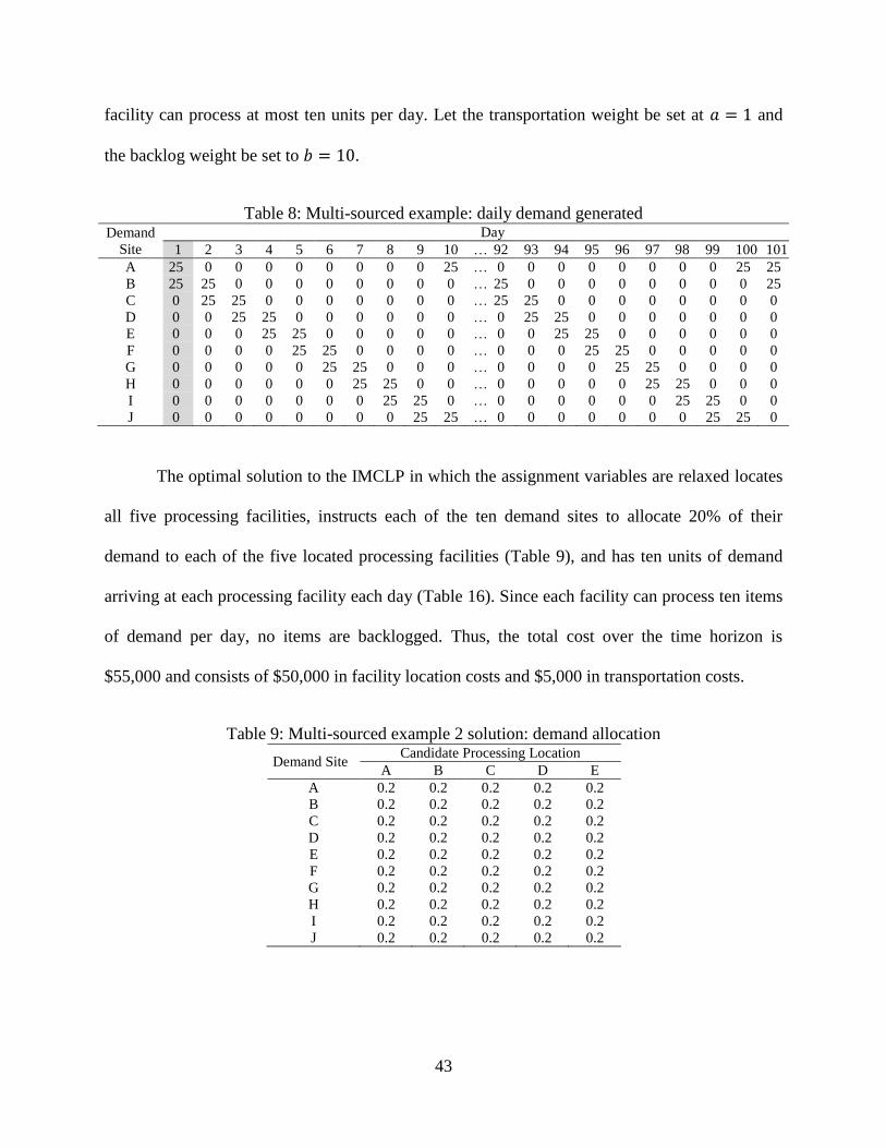
43
facility can process at most ten units per day. Let the transportation weight be set at 𝑎 = 1 and
the backlog weight be set to 𝑏 = 10.
Table 8: Multi-sourced example: daily demand generated Demand
Site
Day
1 2 3 4 5 6 7 8 9 10 … 92 93 94 95 96 97 98 99 100 101
A 25 0 0 0 0 0 0 0 0 25 … 0 0 0 0 0 0 0 0 25 25
B 25 25 0 0 0 0 0 0 0 0 … 25 0 0 0 0 0 0 0 0 25
C 0 25 25 0 0 0 0 0 0 0 … 25 25 0 0 0 0 0 0 0 0
D 0 0 25 25 0 0 0 0 0 0 … 0 25 25 0 0 0 0 0 0 0
E 0 0 0 25 25 0 0 0 0 0 … 0 0 25 25 0 0 0 0 0 0
F 0 0 0 0 25 25 0 0 0 0 … 0 0 0 25 25 0 0 0 0 0
G 0 0 0 0 0 25 25 0 0 0 … 0 0 0 0 25 25 0 0 0 0
H 0 0 0 0 0 0 25 25 0 0 … 0 0 0 0 0 25 25 0 0 0
I 0 0 0 0 0 0 0 25 25 0 … 0 0 0 0 0 0 25 25 0 0
J 0 0 0 0 0 0 0 0 25 25 … 0 0 0 0 0 0 0 25 25 0
The optimal solution to the IMCLP in which the assignment variables are relaxed locates
all five processing facilities, instructs each of the ten demand sites to allocate 20% of their
demand to each of the five located processing facilities (Table 9), and has ten units of demand
arriving at each processing facility each day (Table 16). Since each facility can process ten items
of demand per day, no items are backlogged. Thus, the total cost over the time horizon is
$55,000 and consists of $50,000 in facility location costs and $5,000 in transportation costs.
Table 9: Multi-sourced example 2 solution: demand allocation
Demand Site Candidate Processing Location
A B C D E
A 0.2 0.2 0.2 0.2 0.2
B 0.2 0.2 0.2 0.2 0.2
C 0.2 0.2 0.2 0.2 0.2
D 0.2 0.2 0.2 0.2 0.2
E 0.2 0.2 0.2 0.2 0.2
F 0.2 0.2 0.2 0.2 0.2
G 0.2 0.2 0.2 0.2 0.2
H 0.2 0.2 0.2 0.2 0.2
I 0.2 0.2 0.2 0.2 0.2
J 0.2 0.2 0.2 0.2 0.2

44
Table 10: Multi-sourced example 2 solution: total demand arriving at processing facility
Processing
Facility
Day
1 2 3 4 5 6 … 101
A 0 10 10 10 10 10 … 10
B 0 10 10 10 10 10 … 10
C 0 10 10 10 10 10 … 10
D 0 10 10 10 10 10 … 10
E 0 10 10 10 10 10 … 10
Note that since ten demand sites are multi-sourced and five facilities are located, this
example shows that the number of multi-sourced sites exceeds the number of facilities located
minus one. Furthermore, we identify that there are no alternative optimal solutions in which
fewer demand sites are multi-sourced by adding the following constraints to formulation (2.2) -
(2.4) and (3.2) - (3.8), resolving the model, and observing an optimal cost that is higher than
$55,000.1 We let 𝑁𝑖𝑗 be a binary variable that takes the value of one if demand site 𝑖 allocates
any of its demand to facility 𝑗 (and zero otherwise), 𝐸𝑖 be a binary variable that takes the value of
one if demand site 𝑖 is multi-sourced (and zero otherwise) and add the constraints:
𝑁𝑖𝑗 ≥ 𝑌𝑖𝑗 ∀𝑖 ∈ 𝐼; 𝑗 ∈ 𝐽 (3.12)
∑ 𝑁𝑖𝑗𝑗∈𝐽 ≤ 1 + (|𝐽| − 1)𝐸𝑖 ∀𝑖 ∈ 𝐼 (3.13)
∑ 𝐸𝑖𝑖∈𝐼 ≤ |𝐼| − 1 ∀𝑖 ∈ 𝐼 (3.14)
Constraints (3.12) ensure that the variable 𝑁𝑖𝑗 is one if demand site 𝑖 allocates any of its
demand to facility 𝑗). Then, the left hand side of constraint (3.13) counts the number of facilities
to which demand site 𝑖 allocates its demands. If it allocates demands to more than one facility,
demand site 𝑖 is multi-sourced and variable 𝐸𝑖 must take on a value of one. Finally, constraints
(3.14) ensure that at least one demand site is not multi-sourced. We note that the right hand side
of constraint (3.14) represents the maximum number of multi-sourced demand sites that are
allowed, and can be changed to any non-negative value the user desires. For example, if we want
1 For the example data, the optimal cost of the solution to the IMCLP model in which we ensure at least one demand
site is not multi-sourced is $83,150.

45
to ensure that the number of multi-sourced sites does not exceed the number of located
processing facilities minus one, the right hand side of constraint (3.14) can be replaced by
∑ 𝑋𝑗𝑗∈𝐽 − 1.1 Adding constraints (3.12) - (3.14) to formulation (2.2) - (2.4) and (3.2) - (3.8)
results in a larger objective function value for this problem instance, thereby showing that there
is no alternate optimum in which fewer demand nodes are multi-sourced.
3.4 Computational Results
We now provide computational results for the IMCLP. In particular, we test the
sensitivity of the IMCLP solution time as the size of the problem instance increases and compare
the optimal IMCLP solution to that of the CFLP. The models are coded in AMPL and the MIP
problems are solved using CPLEX 12.2.0 on an Intel 3.20 GHz Xeon CPU with 8 GB of
memory.
Model data are generated based on 2010 U.S. census population data from the 500 largest
U.S. counties. In the discussion that follows, we refer to counties as nodes and refer to a node in
terms of its population rank. (i.e., The largest county, Los Angeles, CA, has rank 1 while the
500th
largest county, Boone, KY, has rank 500.) Multiple problem instances are created by
varying the number of demand-generating sites and candidate processing facilities. The data
instances use the largest (with respect to the population) nodes as demand-generating sites and
possible candidate facility locations. For example, an instance with 100 candidate locations
includes the 100 largest nodes while a data instance with 150 candidate locations includes the
same nodes as the 100 candidate location dataset plus the next 50 largest nodes. From these data
instances we generate the necessary model parameters as follows.
1 For the example data, the optimal cost of the solution to the IMCLP model in which we restrict the number of
multi-sourced demand nodes to be no greater than the number of located processing facilities minus 1 is $108,950

46
Unless otherwise noted, for each demand site 𝑖 ∈ 𝐼, discrete, random daily demands are
generated for a 100 day time horizon (plus the warm-up days required for initialization) from a
Poisson distribution with a mean of 1/10,000 of the county population, 𝜌𝑖. To remain consistent,
the average daily demand at site 𝑖 ∈ 𝐼 is set to 1
10,000𝜌𝑖 in the CFLP instances. The second and
third columns in Table 11 display the population and corresponding average daily demand
parameter used to generate the daily Poisson distributed demands for the five largest demand
sites, respectively. Demands were generated at this rate seven days a week at all the demand
sites, and the resulting sample statistics are presented in columns four and six of Table 11.
Additionally, Table 12 provides further information regarding the population range of the 500
largest counties.
Table 11: Demand statistics for 5 largest demand sites
Demand Site Population
(𝜌𝑖)
Theoretical
Average Daily
Demand
(1
10,000𝜌𝑖)
Sample
Average
Daily Demand
Theoretical
Standard
Deviation of
Demand
Sample
Standard
Deviation of
Demand
Los Angeles, CA 9,818,605 982 984.8 31.3 29.3
Cook, IL 5,194,675 519 519.6 22.8 22.4
Harris, TX 4,092,459 409 410.1 20.2 20.4
Maricopa, AZ 3,817,117 382 380.8 19.5 19.1
San Diego, CA 3,095,313 310 309.0 17.6 16.0
Table 12: Population Range of 500 Largest US Counties Node Rank Max. 𝜌𝑖 Min. 𝜌𝑖 Avg. 𝜌𝑖 St Dev 𝜌𝑖
1-50 9,818,605 916,924 1,833,113 1,442,311
51-100 916,829 618,754 754,214 91,285
101-150 603,403 434,972 511,279 48,884
151-200 432,552 316,236 373,976 36,902
201-250 315,335 255,793 284,748 16,693
251-300 255,755 203,206 229,034 16,506
301-350 203,065 174,528 189,518 9,097
351-400 174,214 154,358 163,353 5,515
401-450 153,990 136,484 144,544 5,696
451-500 136,146 118,811 127,719 5,082
Distances between nodes are calculated based on the Great Circle Distance (e.g.,
Weisstein (2016)). We use this distance to calculate the travel time between nodes under the

47
assumption that it takes one day to process the outgoing order at the demand-generating site and
one day to transport an item 100 miles. The travel times are integer valued. Thus, if the Great
Circle Distance between two nodes is 402 miles, the travel time between the nodes is six days
(⌈402/100⌉ = 5 days for traveling plus one day for processing). Under this assumption,
demands are never processed on the day they originate, in accordance with the discussion in
Section 3.2. For example, suppose a processing facility is located at node A and also that the
demand generated at node A is assigned to be processed at node A. All of the demands that
originate at node A on day 𝑑 will arrive to be processed at node A on day 𝑑 + 1. Such a scenario
resembles that of a postal service policy in which mail carriers collect mail from various houses
and businesses during the day and bring the collected mail to the post office at the end of the
business day. If we assume that there is no night shift at the post office, the mail must wait until
the next business day to be processed. Thus, the effective travel time plus processing time is one
day.
The daily facility location costs are calculated by specifying a daily base cost plus an
additional cost calculated from the associated demand (population) generated at that location.
Specifically, we use the formula
𝑧 + 𝑤𝜌𝑗
to generate the daily facility location cost for each facility 𝑗 ∈ 𝐽, where 𝑧 denotes the daily base
fixed cost and 𝑤 is the population weight. For the instances that follow, we let the daily base
fixed cost be 𝑧 = $10,000 and the weight be 𝑤 = $0.0001. For example, Los Angeles, CA,
which has a population of 9,818,605, has a daily fixed cost of $10,000 + $0.0001 ∗
9,818,605 = $10,982 while Du Page, IL, which has a population of 916,924, has a daily fixed
cost of $10,000 + $0.0001 ∗ 916,924 = $10,092. We note that the population weight 𝑤 greatly

48
affects which facilities are located; larger values of 𝑤 result in greater disparities between the
cost of locating a facility in the most populous county (i.e., Node 1- Los Angeles, CA) and in a
less populous county (e.g., Node 50, Du Page, IL). We direct the interested reader to Appendix B
for an analysis of the effect of the population weight on the optimal solution.
We assume that each facility, regardless of its location, has a uniform capacity of one
fifth of the total average daily demand, rounded up to the nearest hundred. Thus, the capacity of
each processing facility depends on which (and how many) demand nodes are considered. For
example, since the 50 largest demand sites generate a daily average of 9,166 units of demand and
1,833.2 is one fifth of 9,166, each candidate processing facility has a daily processing capacity of
1,900 units. Furthermore, the capacity of each processing facility in an instance with 50 demand
nodes is less than the capacity of each processing facility in, for example, a 100 demand node
instance since the latter instance generates more total average demand each day. The specific
capacity levels of the problem instances used in this chapter are reported in Table 13.
Table 13: Daily processing capacity per candidate facility
# Demand
Nodes
Total Average
Daily Demand
1/5 Total Average
Daily Demand
Daily Capacity
per Candidate
Facility
Daily Capacity % of
Total Average Daily
Demand
50 9,166 1833.2 1900 20.7%
100 12,936 2587.2 2600 20.1%
150 15,491 3098.2 3100 20.0%
200 17,360 3472.0 3500 20.2%
250 18,787 3757.4 3800 20.2%
300 19,929 3985.8 4000 20.0%
350 20,878 4175.6 4200 20.1%
400 21,696 4339.2 4400 20.3%
450 22,421 4484.2 4500 20.0%
500 23,054 4610.8 4700 20.4%
If there is sufficient capacity in the system for the CFLP to accommodate all demands,
then, in expectation, there will be sufficient capacity in the system for the IMCLP model to
accommodate all demands. This is because the processing capacities are the same in the two

49
models and the daily demands in the IMCLP model are realizations of a random distribution with
constant mean equal to the mean used in the CFLP. If the underlying demand process is time
dependent (i.e., the mean demand at a location changes with time), then a different model must
be applied [Drezner and Wesolowsky, 1991].
Conversion factors 𝑎 and 𝑏 are chosen to limit the number of items held in backlog from
day to day to a reasonable value and will be specified in each problem instance individually. We
consider 𝑎 and 𝑏 values to be reasonable if the backlog does not grow without bound at any
processing facility when five facilities are located.
Unless otherwise noted, the following results are generated using instances constructed
using the aforementioned method.
3.4.1 Empirical Number of Multi-Sourced Demand Nodes
To compare the theoretical results regarding the number of multi-sourced demand sites
discussed in Section 3.3.3 with empirical results, we investigate the percent of demand sites that
are multi-sourced for numerous problem instances. Each problem instance uses a time horizon of
100 days and the 50 most populous counties as candidate facility locations. The number of
demand sites varies in increments of 50 to 500. The results in Table 14 indicate that although in
theory all of the demand sites could be multi-sourced, no more than 8% of the demand sites were
multi-sourced in the optimal solution of the data instances we considered. Moreover, all but one
of the optimal solutions had at most 3% of the demand sites multi-sourced. Nevertheless, the
instances with 300, 400, and 450 demand sites again confirm that the number of multi-sourced
sites can exceed the number of facilities located minus one in the optimal solution.1
1 Since there may be multiple alternative optima, we note that the number of multi-sourced demand nodes reported
in Table 14 for each problem instance is the minimum number of multi-sourced demand nodes across all

50
Table 14: Number of multi-sourced demand sites; 𝑎 = 1, 𝑏 = 3
# Demand
Nodes
# Candidate
Nodes
# of
Multi-Sourced
Demand Nodes
% of Demand
Nodes that are
Multi-Sourced
# Open
Facilities
Rank of Open
Facilities
50 50 4 8.00% 5 2,3,6,7,13
100 50 3 3.00% 6 11,16,20,25,30,33
150 50 4 2.67% 6 11,16,25,33,35,43
200 50 5 2.50% 6 9,11,25,26,30,33
250 50 3 1.20% 6 10,11,15,16,25,35
300 50 6 2.00% 6 9,11,15,20,25,35
350 50 4 1.14% 6 2,9,11,20,25,48
400 50 9 2.25% 6 2,9,11,20,25,48
450 50 8 1.78% 6 2,9,11,20,25,48
500 50 5 1.00% 6 2,9,11,20,25,48
Using the 50 demand, 50 candidate facility locations instance as a base case, we increase
the backlog weight, 𝑏. Our results indicate that the number of multi-sourced demand sites does
not increase until 𝑏 > 100. However, as 𝑏 increases past 100, the number of multi-sourced
demand sites significantly increases. The number of located processing facilities remains
constant at five located facilities. However, in general, the backlog weight can change the
number of located facilities; typically, an additional facility will be located to accommodate
excess backlog if the backlog weight is sufficiently high. The results are presented in Figure 4.
Figure 4: Effect of increasing backlog weight, 50 demand & candidate nodes, 100 days, 𝑎 = 1
corresponding optimal solutions. This was verified by observing a higher optimal cost when we imposed a constraint
that restricted the number of multi-sourced demand nodes to be less than the number reported in the fifth column of
Table 14.
0
1
2
3
4
5
6
7
8
9
10
0%
10%
20%
30%
40%
50%
60%
70%
80%
90%
100%
100 200 300 400 500 600 700 800 900 1000
Num
ber
of
Fac
ilit
ies
Op
ened
% o
f D
eman
d N
od
es
that
are
Mult
i-S
ourc
ed
Backlog cost (b)
Effect of Increasing b on the % of Multi-Sourced Demand Nodes
Number Opened
% Multi Sourced

51
3.4.2 Comparison to CFLP
Next, we compare the effect of incorporating capacity into facility location models via
the CFLP and the IMCLP. We find that the CFLP and IMCLP generally do not have the same
optimal solutions in terms of the location and allocation decisions. In fact, the two models can
choose to not only locate different processing facilities, but also locate a different number of
processing facilities. In the following paragraph we present one such example in which the
CFLP locates fewer facilities than the IMCLP. While the demand data used in the CFLP and
IMCLP are generated from the same daily demand mean, the IMCLP differs from the CFLP in
that if the total demand that arrives at a processing facility exceeds the processing capacity, a
penalty cost is incurred because the unprocessed demand must wait in backlog to be processed at
a later date. If this cost is sufficiently high, the IMCLP model will choose to locate an additional
facility to mitigate the effect of the backlog penalty costs.
For the results in this section, random daily demands for the IMCLP were generated from
a Poisson distribution with a mean of 1/5,000 of the node population. Since the CFLP requires as
input a generic daily demand value, we set the average daily demand for the CFLP to be 1/5,000
of the demand node population to be consistent with the manner in which the IMCLP data were
generated. The facility capacities, fixed location costs, and travel times between sites were
generated in the manner described earlier in Section 3.4 except that a weight of 𝑤 = 0.01 was
used for the fixed location costs. In this case, the daily facility location costs of the candidate
processing facilities range from $108,186 (Node 1: Los Angeles, CA) to $19,169 (Node 50: Du
Page, IL).
We ran the IMCLP and CFLP models for the 50 demand, 50 candidate node problem
instance with a 100 day time horizon. The conversion factors of 𝑎 = 1 and 𝑏 = 100 were used.

52
CFLP Model
DuPage, IL
Westchester, NY
Travis, TX
Pima, AZ
Fresno, CA
The traditional CFLP model located processing facilities in Fresno, CA; Pima, AZ; Travis, TX;
DuPage, IL; and Westchester, NY while the IMCLP located an additional facility in Orange, FL.
Note that the CFLP located five facilities while the IMCLP located six. The optimal location and
allocation assignments of the two models can be seen in Figure 5 and Figure 6. The large boxes
denote located facilities and the lines connect each demand site to its assigned processing
facility. In both the CFLP and IMCLP solutions the demand sites were not necessarily assigned
to the nearest located facility. For example, in the optimal CFLP solution, Fulton, GA is closer to
DuPage, IL (589 miles, seven days) but was assigned to Travis, TX (818 miles, ten days) and in
the IMCLP solution, Salt Lake, UT was assigned to Travis, TX (1068 miles, 12 days) although it
is much closer to Fresno, CA (502 miles, seven days). These two demand sites are identified in
Figure 5 and Figure 6 by a dotted circle.
Figure 5: Optimal CFLP Solution; 50 demand & candidate nodes, 𝑎 = 1; mean daily demand=1/5000 node population, 𝑤 = 0.01

53
DuPage, IL
Westchester, NY
Travis, TX
Pima, AZ
Fresno, CA
Orange, FL
IMCLP Model
Figure 6: Optimal IMCLP solution; 50 demand & candidate nodes, 𝑎 = 1, 𝑏 = 100;
mean daily demand=1/5000 node population, 𝑤 = 0.01
As we will discuss in Section 3.4.3, preliminary results show that the CFLP solves much
faster than the IMCLP. Therefore, as we did with a small example in Section 3.3., we again
investigate the effect on the optimal objective function value of the IMCLP if demand allocations
are given by the solution to the capacitated facility location problem as the relative cost of
backlog to transportation cost varies. For this analysis we fix the transportation weight at 𝑎 = 1
and vary the backlog weight, 𝑏. The results indicate that the solution obtained by using the CFLP
allocations can provide very poor approximations to the optimal solution of the IMCLP,
particularly as it becomes more costly to hold items in backlog. This is to be expected since the
CFLP does not incorporate backlog in the objective function. For example, when 𝑎 = 𝑏 = 1 the
optimal locations determined by the IMCLP and CFLP are the same. However, if a company
experiences unit daily backlog carrying costs that are 100 times as much as the unit
transportation costs, the company would see an undesirable total cost increase of 9% if the
location and allocation decisions are determined via the CFLP rather than by the IMCLP. A
major contributor to the cost difference between the two models is that the optimal IMCLP

54
solution locates six facilities whereas the corresponding CFLP solution only locates five
facilities. This is in part due to the fact that the backlogging costs that would be accumulated if
only five facilities were located can be mitigated by locating an additional processing facility.
We also note that the optimal CFLP solution clearly does not change as the backlog weight, 𝑏,
varies since backlog is not accounted for in the CFLP.
3.4.3 Effect of Problem Size
In this section we investigate the effect of problem size on solution times by increasing
the number of demand and candidate nodes simultaneously, increasing the number of demand
nodes only, and increasing the time horizon while keeping the number of demand and candidate
nodes constant. We present the solution time in seconds or, if a provably optimal solution could
not be found within one hour, we present the percent optimality gap as obtained by CPLEX
12.2.0.
Increasing the Number of Nodes
We increase the number of demand and candidate nodes simultaneously and report the
solution times and processing facilities located for the CFLP, IMCLP, and IMCLP with the
assignment variables relaxed from binary (i.e., Relaxed IMCLP). The solution time or optimality
gap after one hour for data instances ranging from 50 to 500 demand and candidate nodes are
presented in Table 15. We report a 100% optimality gap for problem instances in which no
feasible solution is found within one hour. We find that the CFLP solves much quicker than both
the IMCLP and Relaxed IMCLP problems. This is expected due to the additional constraints and
variables in the IMCLP that track the daily activity of the processing facilities.

55
Table 15: Solution times (in seconds) or % optimality gap (indicated by shading) within 1 hour
using a generic solver; 𝑎 = 1, 𝑏 = 3 # Demand & Candidate Nodes CFLP IMCLP Relaxed IMCLP
50 0.52 6.35 8.11
100 192.74 1544.11 496.49
150 0.58% 3.70% 1.55%
200 0.93% 3.75% 2.26%
250 1.69% 3.54 % 2.99%
300 2.53% 5.66% 4.77%
350 2.02% 5.69% 3.13%
400 2.65% 51.26% 3.29%
450 5.14% 92.10% 100%
500 2.99% 100% 100%
Preliminary results indicate that the IMCLP model tends to locate processing facilities at
nodes corresponding to larger populations (and therefore at the nodes that generate the largest
demand). Thus, we reduce the set of candidate processing facilities by eliminating the candidate
nodes with the lowest population to obtain an approximate solution.
We begin by using the 100 demand, 100 candidate node instance with 100 days of daily
demand data, 𝑎 = 1, and 𝑏 = 3 to illustrate the results. We consider various candidate node sets,
including the set in which all 100 of the demand nodes also serve as candidate nodes and the set
with only the nodes corresponding to the ten largest populations. The tradeoff in solution time
and cost is displayed in Figure 7. The cost increase is compared to the optimal cost when all 100
nodes are in the candidate node set. As expected, as the number of candidate nodes decreases,
the solution time also decreases while the cost increases. We find that a similar result holds for
the CFLP.

56
Figure 7: Effect of changing number of candidate nodes; 100 demand & candidate nodes, 100
days, 𝑎 = 1, 𝑏 = 3
For example, the optimal solution using all 100 nodes as candidate nodes locates
processing facilities at the 11th
, 16th
, 20th
, 25th
, 30th
, and 60th
largest nodes (i.e., Riverside, CA;
Tarrant, TX; New York, NY; Sacramento, CA; Hillsborough, FL; and Macomb, MI,
respectively) and takes 1544.11 seconds to solve. However, if we restrict the set of candidate
nodes to include only the 30 nodes with the largest population, the solution time is reduced to
45.29 seconds (a 97% reduction) and the cost of the solution obtained is only 0.0134% more than
the optimal solution. The 30 candidate node problem locates all but one of the same processing
facilities as does the problem with 100 candidate nodes; the 60th
largest county (i.e., Macomb,
MI) located in the 100 candidate node problem is replaced by the 15th
largest county (i.e.,
Wayne, MI) in the 30 candidate node problem.
Since reducing the size of the candidate node set was beneficial in terms of the solution
time with only a minimal increase in cost for the 100 demand node problem instance, we next
vary the number of demand nodes from 50 to 500 in intervals of 50. The transportation and
backlog weights are the same as those listed in Table 15. In Figure 8 we display the IMCLP
optimality gap after one hour of run time when all of the demand nodes are candidate nodes, as
well as when only the 50 and 100 largest demand nodes are candidate nodes. The IMCLP data
0%
1%
2%
3%
4%
5%
6%
0
200
400
600
800
1000
1200
1400
1600
1800
0% 20% 40% 60% 80% 100%
% O
ver
Op
tim
al C
ost
So
luti
on
Tim
e (s
eco
nd
s)
% of Demand Nodes used as Candidate Nodes
Effect of Changing Number of Candidate Nodes
US Data, 100Nodes, % over
Solution Time
% Over Optimal

57
referenced in Table 15 is used for the “All Nodes” case. It is clear that reducing the size of the
candidate node set to include only the 50 or 100 largest nodes significantly improves the solution
progress within one hour.
Figure 8: IMCLP solution progress as size of candidate node set varies; 100 days; 𝑎 = 1, 𝑏 = 3
Additionally, Figure 8 suggests that restricting the size of the candidate set to the 50
largest nodes usually does not provide a significant reduction in the solution progress when
compared to that of the largest 100 node candidate node set. An exception to this is the 500
demand node instance, which solves to optimality when only the 50 largest nodes are in the
candidate node set but has a 20.8% optimality gap after one hour when the 100 largest nodes are
in the candidate node set.
When the same number of demand and candidate node instances are run for the CFLP we
find that the resulting optimality gaps after one hour are reduced (see Figure 9). Of particular
note are the instances consisting of 350-500 demand nodes when all of the demand nodes are
candidate nodes as well. In the problem instance with 500 candidate nodes, the CFLP reported an
optimality gap of 6.21% within one hour while the IMCLP does not find a feasible solution in
0%
20%
40%
60%
80%
100%
0 100 200 300 400 500
% O
pti
mal
ity G
ap a
fter
1 H
our
Number of Demand Nodes
All Nodes
Largest 100 Nodes
Largest 50 Nodes
IMCLP Solution Progress as Size of Candidate Node Set Varies

58
the same time frame. We note that the scale of the y-axis in Figure 9 is different than that of
Figure 8.
Figure 9: CFLP solution progress as size of candidate node set varies; 𝑎 = 1
Increasing the Number of Days in the Planning Horizon
Since Table 15 indicates that the 50 demand, 50 candidate node instance produced an
optimal solution relatively quickly for 100 days of daily demand data, we investigate the
sensitivity of the optimal location solutions with respect to the planning time horizon. The time
horizon varies from 10 to 4,000 days and the transportation and backlog weights are the same as
those listed in Table 15. The daily demands in each problem instance are independent of the
demands in the other problem instances. For example, the daily demands for the ten days in the
ten day time horizon instance are different than the first ten days in the 4,000 day time horizon
instance. Additionally, we report whether the optimal facilities that are located change as the
number of days increase. Figure 10 displays the solution time for the problem. All problem
instances were solved to optimality within one hour.
0%
1%
2%
3%
4%
5%
6%
7%
0 100 200 300 400 500
% O
pti
mal
ity G
ap a
fter
1 H
our
Number of Demand Nodes
All Nodes
Largest 100 Nodes
Largest 50 Nodes
CFLP Solution Progress as Size of Candidate Node Set Varies

59
0
500
1000
1500
2000
2500
3000
3500
0 500 1000 1500 2000 2500 3000 3500 4000
So
luti
on T
ime
(Sec
ond
s)
Time Horizon (Days)
Effect of Increasing Time Horizon
Figure 10: Effect of increasing time horizon, 50 demand & candidate nodes, 𝑎 = 1, 𝑏 = 3
We find that the optimal processing locations are relatively insensitive to the length of the
time horizon. The optimal locations remain constant for time horizons of 100 to 3,500 days. For
various problem instances with a time horizon of less than 100 days and the problem instance
with 4,000 days a slight change in the optimal facility locations occurs. In particular, for these
problem instances, it is optimal to locate a processing facility in Riverside County rather than in
Orange County. However, we note that these two counties are neighboring counties in California
and, as such, the increase in cost of locating the processing facility in Orange County rather than
in Riverside County is only 0.0001237% in the 4,000 day instance. We also note that the solution
to the IMCLP instances that locate a facility in Riverside County is precisely the optimal solution
to the corresponding CFLP problem in terms of the processing facilities located.
3.5 Chapter Summary
We have argued that the hard capacity constraints that are often employed in location
modeling are unrealistic since facility managers have numerous operational tools that allow a
facility to accept items in excess of the stated processing capacity level. As such, we have

60
developed a new approach to modeling capacity constraints in a facility location and allocation
model that permits storing excess demand as backlog to be processed at a later date.
We reported the difference in facility locations, demand allocations, and total cost
between the CFLP and our approach. In particular, we have shown that the CFLP and IMCLP
often do not locate the same facilities (and in some instances they locate a different number of
facilities), and therefore also do not allocate demands to the same processing facilities. Since the
CFLP does not incorporate the cost of backlogged demand, the CFLP underestimates the total
cost, but also results in solutions with a higher total cost (as compared to the IMCLP) when the
demand is realized and backlogging is allowed in practice. Such an underestimate could have
significant implications on budget predictions.
Additionally, we compared the effect of increasing the problem size by increasing the
number of demand and candidate nodes, only the number of demand nodes, and the time
horizon. Computational results indicated that increasing the number of demand and candidate
nodes simultaneously adds a significant burden on the IMCLP solution time. However, for the
instances considered, we found that by limiting the candidate nodes to include only a subset of
the largest populated demand nodes, we significantly reduced the solution time and still obtained
a solution that is near optimal to the original problem. We also found that the optimal locations
to the IMCLP are relatively insensitive to the length of the time horizon for the problem
instances considered. Detailed analysis regarding the effect of a wider variety of model
parameters on these conclusions is left as an area of future research.
A key benefit of the IMCLP model is that it incorporates a penalty cost associated with
the reality that on some days the total amount of demand arriving at a processing facility may
exceed the daily processing capacity. The IMCLP formulation inherently assumes that demands

61
do not expire; demands can be postponed indefinitely as long as the penalty cost is paid.
However, we realize that in many situations this is not realistic and therefore we presented
additional constraints that can be added to the IMCLP to ensure demands are processed within a
specified amount of time.
Furthermore, the IMCLP can use a dataset as a direct input into the model rather than
specifying deterministic demands at an aggregate level by using parameter estimation
techniques. This allowed us to explicitly incorporate the variation in and the possibly correlated
nature of demands. As a result, variations of this model have the potential to reveal operating
policies that take advantage of spatial and temporal correlations in demand that are not evident in
current facility location models. An example of such a variation is an allocation policy that varies
by day of the week to take advantage of regular daily fluctuations in demand and/or variations in
capacity that result from operating the processing facility for different hours each day of the
week. Demand site 𝑖 ∈ 𝐼 may allocate its demands to facility 𝑗1 ∈ 𝐽 on weekends and to facility
𝑗2 ∈ 𝐽 on weekdays, for example. Such extensions are presented in the next chapter.

62
CHAPTER 4: A Cyclic Allocation Model for the IMCLP
4.1 Motivation
Processing facilities can have many different operational policies, even within a single
organization. For example, a portion of the facilities may operate at full capacity 24 hours per
day, seven days a week, others may reduce their processing capacity on weekends, and some
may only be open on weekdays. In this chapter we show that allowing demands at a particular
demand-generating site to be allocated to multiple processing facilities in a cyclic manner that
accounts for capacity levels that vary by day-of-the-week can be a cost effective operational tool.
Furthermore, such an allocation method affords the model flexibility to utilize an allocation
policy that captures systematic day-of-the-week demand patterns, even when all processing
centers are operational at identical times.1
Thus, we expand the IMCLP to include a cyclic demand allocation approach. While the
IMCLP restricts each demand site to allocate its demand to a single processing facility for the
entire demand horizon, we now relax that assumption and allow demands to be allocated to
multiple processing facilities over a specific time frame (e.g., a week), but to a single facility
each day. As an example of such a system, blood is often drawn at local clinics and sent for
testing at more regional centers [Saveh-Shemshaki, 2012]. If some testing centers operate five
days per week and others operate seven days per week, a day-of-the-week assignment policy can
reduce costs and improve the time-to-processing relative to a single assignment policy. For
1 A majority of the content of this chapter has been published in Maass and Daskin (2017).

63
example, a clinic may send its blood samples to arrive at one testing facility (that is closed on
weekends) on Mondays through Fridays and to another testing facility (that is open on
weekends) on Saturdays and Sundays. This allows for a more efficient use of the processing
system by mitigating the amount of unprocessed blood samples that are held in cold storage over
the weekend.
4.2 Model Formulation
The following model formulation generates cyclic day-of-the-week assignments, which
account for the deterministic day-to-day variation in processing capacity levels as well as
deterministic cyclic patters and correlations among the demand sites.
Let the set 𝑃 ≔ 0, 1, … , 6 represent the days of the week, where element 𝑝 = 0
represents Saturday, 𝑝 = 1 represents Sunday, etc. In addition to the notation used in the
IMCLP, we also make the following additions. Assume, without loss of generality, that the first
day in 𝐷 is a Sunday to match element 𝑝 = 1 in set 𝑃. Additionally, for each 𝑝 ∈ 𝑃, we can also
generate the set 𝐷𝑝 ≔ 𝑑 ∈ 𝐷: 𝑑 𝑚𝑜𝑑 |𝑃| = 𝑝, 𝑑 > 𝑡∗, which contains the days in the planning
horizon that correspond to the day of the week indicated by 𝑝. For example, if 𝐷 = 1, 2, … , 42
and 𝑡∗ = 1, then 𝐷2 = 2, 9, 16, 23, 30, 37 would represent the set of Mondays in 𝐷. However,
if 𝑡∗ = 2, then we would not include day 2 in the set 𝐷2 = 9, 16, 23, 30, 37.
Note that we assume that the demand rate may vary by day-of-the week, but that it does
not change from week to week. That is, while the realizations of the daily demand for a
particular demand site will fluctuate throughout the planning horizon since they are samples
from a distribution, the realizations are taken from the same distribution each Sunday. However,
a demand site might have a different demand distribution for Mondays than Sundays.

64
In addition to the notation used to formulate the IMCLP, we introduce the following for
the cyclic allocation model:
Sets and Parameters
𝑃 ≔ 0,1, … ,6 Set of cycle days (e.g., days of the week)
𝐷𝑝 ≔ 𝑑 ∈ 𝐷: 𝑑 𝑚𝑜𝑑 |𝑃| = 𝑝, 𝑑 > 𝑡∗ Set of days in 𝐷 corresponding to cycle day 𝑝 ∈ 𝑃 after
the warm-up period
𝑘𝑗𝑝 Capacity of facility 𝑗 ∈ 𝐽 in items processed per day on cycle day 𝑝 ∈ 𝑃
Decision Variables
𝑌𝑖𝑗𝑝 =
1 0
If we ship demands from demand site 𝑖 ∈ 𝐼 to faciliy 𝑗 ∈ 𝐽 on cycle day 𝑝 ∈ 𝑃 Otherwise
With this notation, we formulate the cyclic allocation model as follows:
Formulation
𝑀𝑖𝑛𝑿,𝒀,𝑽,𝑾 (|𝐷| − 𝑡∗)∑ 𝑓𝑗𝑋𝑗𝑗∈𝐽 + 𝑎∑ ∑ ∑ ∑ ℎ𝑖𝑑𝑡𝑖𝑗𝑌𝑖𝑗
𝑝𝑖∈𝐼𝑗∈𝐽𝑑∈𝐷𝑝𝑝∈𝑃 + 𝑏∑ ∑ 𝑉𝑗𝑑𝑗∈𝐽
|𝐷|+1𝑑=𝑡∗+2 (4.1)
𝑆𝑢𝑏𝑗𝑒𝑐𝑡 𝑡𝑜
∑ 𝑌𝑖𝑗𝑝
𝑗∈𝐽 = 1 ∀𝑖 ∈ 𝐼; 𝑝 ∈ 𝑃 (4.2)
𝑌𝑖𝑗𝑝 ≤ 𝑋𝑗 ∀𝑖 ∈ 𝐼; 𝑗 ∈ 𝐽; 𝑝 ∈ 𝑃 (4.3)
𝑉𝑗,𝑑+1 = 𝑉𝑗𝑑 + ∑ ℎ𝑖,𝑑−𝑡𝑖𝑗𝑌𝑖𝑗(𝑑−𝑡𝑖𝑗) 𝑚𝑜𝑑 |𝑃|
𝑖∈𝐼 −𝑊𝑗𝑑 ∀𝑗 ∈ 𝐽; 𝑑 ∈ 𝑡∗ + 1,… , |𝐷| (4.4)
𝑊𝑗𝑑 ≤ 𝑘𝑗𝑝𝑋𝑗 ∀𝑗 ∈ 𝐽; 𝑝 ∈ 𝑃; 𝑑 ∈ 𝐷𝑝 (4.5)
𝑉𝑗,𝑡∗+1 = 𝑣𝑗𝑋𝑗 ∀𝑗 ∈ 𝐽 (3.5)
𝑋𝑗 ∈ 0,1 ∀𝑗 ∈ 𝐽 (2.4)
𝑌𝑖𝑗𝑝 ∈ 0,1 ∀𝑖 ∈ 𝐼; 𝑗 ∈ 𝐽; 𝑝 ∈ 𝑃 (4.6)
𝑉𝑗𝑑 ≥ 0 ∀𝑗 ∈ 𝐽; 𝑑 ∈ 𝑡∗ + 1,… , |𝐷| + 1 (3.7)

65
𝑊𝑗𝑑 ≥ 0 ∀𝑗 ∈ 𝐽; 𝑑 ∈ 𝑡∗ + 1,… , |𝐷| (3.8)
As in the IMCLP, objective function (4.1) minimizes the facility location, transportation,
and backlogging costs by determining the optimal facility locations and demand allocations, as
well as the resulting auxiliary processing and backlog variables. This must be done in a manner
such that each demand site 𝑖 ∈ 𝐼 is assigned to exactly one processing facility 𝑗 ∈ 𝐽 on each cycle
day 𝑝 ∈ 𝑃 (constraints (4.2) and (4.6)). Furthermore, constraints (4.3) state that demands can
only be assigned to located facilities.
Constraints (4.2) - (4.5), (4.6) are the cyclic allocation constraints that correspond to
constraints (2.2), (2.3), (3.3), (3.4), and (3.6), respectively, in the IMCLP. The major difference
between this model and the IMCLP is that this model recognizes that demand sites and
processing facilities may not operate in the same manner every day of the week. The cyclic
formulation facilitates this by allowing the processing facilities to have different processing
capacities throughout the week (i.e., we use capacity parameters 𝑘𝑗𝑝 whereas the IMCLP uses a
constant capacity 𝑘𝑗 every day of the week) and by allowing demand sites to be allocated in a
manner that accounts for the capacity variation and systematic day-to-day variation in the
demands (i.e., we use allocation decision variables 𝑌𝑖𝑗𝑝 rather than the 𝑌𝑖𝑗 variables of the
IMCLP). Such day-of-the-week allocation variables necessitate the inclusion of the sets 𝑃 and
𝐷𝑝, both of which are not present in the IMCLP formulation.
While the daily variation in the processing capacity levels are model inputs, and therefore
known a priori, we can model capacity as a decision variable with an associated cost based on
the amount of capacity employed. Since the capacity level of a processing facility may dictate
the respective staffing needs, such an extension considers both strategic and tactical decisions.

66
We discuss possible formulations of incorporating endogenous capacity flexibility in Section
6.5.1 and leave the analysis of such models as an area of future research.
4.3 Model Properties
We present a small example to illustrate that, from a cost minimization perspective,
incorporating a day-of-the-week assignment policy can perform arbitrarily better than using the
IMCLP model as the cost of backlogging varies.
Consider a system of five clinics that each draw an average of ten blood samples per hour
that they are open. Some clinics are open nine hours each day, while others are open 8, 10, or 12
hours depending on the day of the week. Others are not open on weekends. Each clinic also
serves as a candidate blood testing facility. It takes two days for demands to be shipped from one
site to another for processing and one day for demands to be ready for processing at their own
processing facility. We assume each located processing facility can process up to 100 demands
per day and costs $200 to operate each day. Note that in this example, the processing capacity of
each facility does not vary from day to day; a facility will process blood samples seven days a
week if we choose to locate at that facility, but may only draw blood in the clinic on some of the
days. Poisson distributed demands are generated for a time horizon of 100 days with the daily
distribution mean rate listed in Table 16. The per unit per day transportation cost is fixed at
𝑎 = 2 and we vary the per unit per day backlogging cost, 𝑏.

67
Table 16: Example mean demand rate pattern Sunday Monday Tuesday Wednesday Thursday Friday Saturday
Site 1 80 80 100 100 100 120 120
Site 2 0 90 90 90 90 90 0
Site 3 90 10 10 10 10 10 90
Site 4 90 90 90 90 90 90 90
Site 5 90 90 90 90 90 90 90
For this example, we compare the optimal IMCLP solution to the optimal cyclic
allocation model solution. The computational results indicate that for values of 𝑏 ≥ 30, the
IMCLP locates all five processing facilities and assigns demands to be processed at the site at
which they originate. While the cyclic allocation model also locates all five facilities, it is able to
reduce the total amount of backlog in the system to approximately 10% of the total backlog
accumulated in the IMCLP due to its flexible allocation policy. (As an example, the optimal
cyclic assignments for the case when 𝑏 = 60 are given in Table 17.) The difference in the total
backlog cost (accumulated over the time horizon) is shown in Figure 11 and the resulting cost
difference between the IMCLP and cyclic allocation model is displayed in Figure 12; clearly,
using the IMCLP can become arbitrarily more costly than the cyclic allocation model as 𝑏
increases.
Table 17: Optimal cyclic assignments when 60b — example instance Sunday Monday Tuesday Wednesday Thursday Friday Saturday
Site 1 Site 1 Site 1 Site 1 Site 1 Site 2 Site 1 Site 2
Site 2 Site 3 Site 3 Site 2 Site 3 Site 2 Site 3 Site 1
Site 3 Site 3 Site 5 Site 3 Site 1 Site 3 Site 2 Site 3
Site 4 Site 4 Site 4 Site 4 Site 4 Site 4 Site 4 Site 4
Site 5 Site 5 Site 5 Site 5 Site 5 Site 5 Site 5 Site 5

68
Figure 11: Total backlog—example instance
Figure 12: Total cost—example instance
4.4 Additional Constraints
Although we have shown that the cyclic allocation method has the potential for
significant cost savings as compared to the IMCLP, the optimal solution that results from solving
(2.4), (3.5), (3.7), (3.8) and (4.1) - (4.6) may provide an undesirable allocation decision from a
managerial perspective. For example, an optimal solution may assign demands from a demand
site to a different processing facility each day of the week. (In fact, in the simple 5-node example
of Table 17, Site 3 ships to four of the five located facilities during the week.) This would likely
0
2
4
6
8
10
12
0 20 40 60 80 100
Unit
s o
f B
acklo
g (
in t
ho
usa
nd
s)
Backlog Weight (b)
Total Backlog Accumulated During the Time Horizon
IMCLP
Policy Allocations
0
0.2
0.4
0.6
0.8
1
1.2
0 20 40 60 80 100
To
tal
Co
st (
in m
illi
ons)
Backlog Weight (b)
Total Cost
IMCLP
Policy Allocations

69
require the manager at the demand site to oversee seven individual contracts between the demand
site and the processing facilities. It may be better for the manager’s time to be spent overseeing
only one or two contracts, even if it is more costly to do so. In this section, we describe
additional constraints that may be useful for controlling the allocation policy.
4.4.1 Restricting the Number of Different Allocations
In many cases it is undesirable to allocate demands to a different processing facility each
day of the week. Instead, we may wish to ensure that an individual demand site does not allocate
its items to more than 𝓃 different processing facilities. For any 𝓃 ∈ 1,… , |𝑃|, we do this by
defining 𝑠𝑖𝑗 as a binary variable that takes the value one if demand site 𝑖 ∈ 𝐼 is allocated to
facility 𝑗 ∈ 𝐽 on any day of the week and by adding the constraints
𝑌𝑖𝑗𝑝 ≤ 𝑠𝑖𝑗 ∀𝑖 ∈ 𝐼; 𝑗 ∈ 𝐽; 𝑝 ∈ 𝑃 (4.7)
∑ 𝑠𝑖𝑗𝑗∈𝐽 ≤ 𝓃 ∀𝑖 ∈ 𝐼. (4.8)
While these constraints restrict the number of unique allocations per demand site, they still allow
a demand site’s allocation to change every day by alternating between processing facilities. For
example, if 𝓃 = 2, then the demand site may allocate its demand to one processing facility on
Sundays, Tuesdays, Thursdays, and Saturdays but allocate its demand to another processing
facility on Mondays, Wednesdays, and Fridays.
IMCLP with Cyclic Allocations Model Property: Restricting 𝓃 to take the value of one
reduces the cyclic allocation model to the IMCLP. Since the IMCLP is NP-Hard, the cyclic
allocation model with constraints (4.7) and (4.8) is also NP-Hard.

70
4.4.2 Weekday and Weekend Allocations
While the deterministic processing capacity of a facility may vary every day of the week,
it is very common for some processing facilities to be closed on weekends while others are open
seven days a week. For processing facilities that are only open Monday through Friday (i.e.,
weekdays), any demand that arrives at the facility on the weekend will be held in backlog and
will be available for processing on Monday. Let ℓ1 denote a facility that is only open on
weekdays and let ℓ2 represent a facility that is open seven days of the week. It is reasonable to
assume that a manager at a demand site may wish to follow an allocation policy in which
demands are shipped to arrive at facility ℓ1 during the week and at facility ℓ2 during the
weekend so that the items do not have to wait in backlog at facility ℓ1 due to the weekend
closure. Since travel times are deterministic, we can ensure that such an allocation policy is
adhered to in the following manner.
First, we define the sets 𝑄𝑖𝑗 and 𝑅𝑖𝑗 to represent the set of cycle days for which demand
shipped from demand site 𝑖 ∈ 𝐼 would arrive at processing facility 𝑗 ∈ 𝐽 on the weekend or
during the weekday, respectively. Since the weekend encompasses two days (i.e., Saturday and
Sunday), the set 𝑄𝑖𝑗 contains two elements:
𝑄𝑖𝑗 ≔ (|𝑃| − (𝑡𝑖𝑗𝑚𝑜𝑑|𝑃|))𝑚𝑜𝑑|𝑃|, (|𝑃| − (𝑡𝑖𝑗𝑚𝑜𝑑|𝑃|) + 1)𝑚𝑜𝑑|𝑃|
The remaining days correspond to Monday through Friday and are included in set 𝑅𝑖𝑗:
𝑅𝑖𝑗 ≔ 𝑝 ∈ 𝑃\𝑄𝑖𝑗
The following examples illustrate how the 𝑄𝑖𝑗 and 𝑅𝑖𝑗 sets change relative to the length of the
travel time between a demand site 𝑖 ∈ 𝐼 and a processing facility 𝑗 ∈ 𝐽.
If 𝒕𝒊𝒋 = 𝟏, then demand sent from 𝑖 ∈ 𝐼 on cycle days 6 (Fri.) and 0 (Sat.) will arrive at
processing facility 𝑗 on cycle days 0 (Sat.) and 1 (Sun.). We have

71
𝑄𝑖𝑗 ≔ (7 − (1 𝑚𝑜𝑑 7))𝑚𝑜𝑑 7, (7 − (1 𝑚𝑜𝑑 7) + 1)𝑚𝑜𝑑 7 = 6, 0
as desired. It follows that 𝑅𝑖𝑗 ≔ 1,2,3,4,5.
If 𝒕𝒊𝒋 = 𝟑, then demand sent on cycle days 4 (Wed.) and 5 (Thurs.) will arrive on the
weekend:
𝑄𝑖𝑗 ≔ (7 − (3 𝑚𝑜𝑑 7))𝑚𝑜𝑑 7, (7 − (3 𝑚𝑜𝑑 7) + 1)𝑚𝑜𝑑 7 = 4, 5
𝑅𝑖𝑗 ≔ 0,1,2,3,6
If 𝒕𝒊𝒋 = 𝟏𝟒, then demand sent on cycle days 0 (Sat.) and 1 (Sun.) will arrive on the
weekend:
𝑄𝑖𝑗 ≔ (7 − (14 𝑚𝑜𝑑 7))𝑚𝑜𝑑 7, (7 − (14 𝑚𝑜𝑑 7) + 1)𝑚𝑜𝑑 7 = 0, 1
𝑅𝑖𝑗 ≔ 2,3,4,5,6
Once the sets 𝑄[𝑖, 𝑗] and 𝑅[𝑖, 𝑗] are constructed, we can introduce binary variables
𝑟𝑖𝑗 = 1
0
If demands at 𝑖 ∈ 𝐼 are assigned to facility 𝑗 ∈ 𝐽 on a day such that they would arrive on a weekday Otherwise
and
𝑞𝑖𝑗 = 1
0
If demands at 𝑖 ∈ 𝐼 are assigned to facility 𝑗 ∈ 𝐽 on a day such that they would arrive on a weekend Otherwise
Then, the following two constraints can be implemented to enforce the weekday/weekend
allocation policy:
∑ 𝑌𝑖𝑗𝑝
𝑝∈𝑅𝑖𝑗= 5𝑟𝑖𝑗 ∀𝑖 ∈ 𝐼; 𝑗 ∈ 𝐽 (4.9)
∑ 𝑌𝑖𝑗𝑝
𝑝∈𝑄𝑖𝑗≤ 2𝑞𝑖𝑗 ∀𝑖 ∈ 𝐼; 𝑗 ∈ 𝐽 (4.10)

72
Together with constraints (4.2), constraint (4.9) ensures that demands at 𝑖 ∈ 𝐼 are shipped
to arrive at the same processing facility 𝑗 ∈ 𝐽 on all five weekdays (i.e., Monday – Friday) and
constraints (4.10) allow the demands to arrive at another facility on the weekends. Note that the
inequality constraints of (4.10) do not require that the demand sites ship to multiple processing
facilities; the demand site can always ship its demand to a single processing facility, even if the
processing facility is closed on the weekend. Additionally, simply adding constraints (4.9) and
(4.10) to the model of (2.4), (3.5), (3.7), (3.8) and (4.1) - (4.6) allows a demand site to be
allocated to three processing facilities; it may be assigned to arrive at facility ℓ1 on weekdays,
facility ℓ2 on Saturdays, and facility ℓ3 on Sundays. If we want to ensure that a demand site does
not allocate to a different facility on Saturdays than it does on Sundays, we would let 𝑛 = 2 and
include constraints (4.7) and (4.8). Alternatively, we could let 𝑛 > 2 and add constraints
∑ 𝑞𝑖𝑗𝑗∈𝐽 = 1 ∀𝑖 ∈ 𝐼 (4.11)
to constraint set (4.9) and (4.10) or simply change constraint (4.10) to an equality constraint.
4.4.3 Restricting the Maximum Allowed Travel Time
The optimal cyclic IMCLP solution may assign a demand site 𝑖 ∈ 𝐼 to a processing
facility 𝑗1 ∈ 𝐽 that is relatively close during the week, but assign 𝑖 to another processing facility
𝑗2 ∈ 𝐽 that is very far away on weekends. To address this, we present the following three
additional types of constraints that can be added to formulation (2.4), (3.5), (3.7), (3.8) and (4.1)
- (4.10).

73
Maximal Travel Time Constraints
To ensure that no demand site is assigned to a processing facility that is unreasonably far
away, we can define 𝑡𝑚𝑎𝑥 > 0 as the maximum allowed travel time between demand sites and
processing facilities, and add maximal travel time constraints of the form:
∑ 𝑡𝑖𝑗𝑌𝑖𝑗𝑝 ≤ 𝑡𝑚𝑎𝑥𝑗∈𝐽 ∀𝑖 ∈ 𝐼; 𝑝 ∈ 𝑃 (4.12)
to the model.
Alternatively, we could utilize coverage constraints [Farahani et al., 2012] by introducing
the parameter 𝑐𝑖𝑗 to represent whether the travel time between a demand site and a processing
facility is less than or equal to the maximal travel time allowed; the value of 𝑐𝑖𝑗 is set to one if
𝑡𝑖𝑗 ≤ 𝑡𝑚𝑎𝑥 and 0 otherwise. Then, the following constraints state that on each cycle day, each
demand site must be allocated to a processing facility that reachable within 𝑡𝑚𝑎𝑥 or fewer days:
∑ 𝑐𝑖𝑗𝑌𝑖𝑗𝑝
𝑗∈𝐽 = 1 ∀𝑖 ∈ 𝐼; 𝑝 ∈ 𝑃 (4.13)
Restricting the Time Difference between Weekday and Weekend Allocations
Another method of restricting the travel time is to add constraints that impose a limit, 𝑚,
on the difference in travel time between a demand site and its weekday assignment, and the same
demand site and its weekend assignment. Such constraints are of the form:
𝑡𝑖𝑗1𝑌𝑖𝑗1𝑝1 − 𝑡𝑖𝑗2𝑌𝑖𝑗2
𝑝2 ≤ 𝑚 + 𝑡∗(1 − 𝑌𝑖𝑗2𝑝2) ∀𝑖 ∈ 𝐼; 𝑗1, 𝑗2 ∈ 𝐽; 𝑝1 ∈ 𝑄[𝑖, 𝑗1]; 𝑝2 ∈ 𝑅[𝑖, 𝑗2]. (4.14)
For example, when 𝑚 = 0, demands at site 𝑖 ∈ 𝐼 must take exactly the same number of days to
travel from 𝑖 to their weekend (i.e., Saturday, Sunday, or both) processing facility 𝑗1 ∈ 𝐽 as it
does to travel from 𝑖 to their weekday processing facility 𝑗2 ∈ 𝐽.

74
Closest Assignment Constraints
We consider closest assignment constraints as another method of reducing the difference
in travel time between weekday and weekend assignments. Rather than restricting a demand site
to be assigned to the closest located facility, we allow the demand site to be assigned to one (or
two, in the case of weekday/weekend assignments with 𝓃 = 2) of the 𝜍 closest located facilities.
This is achieved by defining 𝐺𝑖𝑗 as a binary variable that takes the value of one if facility 𝑗 ∈ 𝐽
is the 𝜍 closest located facility to demand site 𝑖 and adding the following constraints:
∑ 𝜍𝐺𝑖𝑗|𝐽|=1 + 1 ≤ ∑ 𝜍𝐺𝑖𝑙
|𝐽|=1 + |𝐽|(1 − 𝑋𝑙) ∀𝑖 ∈ 𝐼; 𝑗 ∈ 𝐽; 𝑙 ∈ 𝑗 ∈ 𝐽|𝑡𝑖𝑗 < 𝑡𝑖 (4.15)
∑ ∑ 𝐺𝑖𝑙𝑙∈𝐽:𝑡𝑖𝑙<𝑡𝑖𝑗|𝐽|=1 + 1 ≤ ∑ 𝜍𝐺𝑖𝑗
|𝐽|=1 + |𝐽|(1 − 𝑋𝑗) ∀𝑖 ∈ 𝐼; 𝑗 ∈ 𝐽 (4.16)
∑ 𝐺𝑖𝑗|𝐽|=1 ≤ 𝑋𝑗 ∀𝑖 ∈ 𝐼; 𝑗 ∈ 𝐽 (4.17)
∑ 𝐺𝑖𝑗𝜍=1 ≥ 𝑌𝑖𝑗
𝑝 ∀𝑖 ∈ 𝐼; 𝑗 ∈ 𝐽, 𝑝 ∈ 𝑃 (4.18)
Constraints (4.15) establish that if two facilities 𝑗 ∈ 𝐽 and 𝑙 ∈ 𝐽 are located, and the
transportation time between facility 𝑗 and demand site 𝑖 ∈ 𝐼 is less than that between facility 𝑙
and 𝑖, then 𝑗 will be assigned a lower rank in relation to demand site 𝑖 than 𝑙. Constraints (4.16)
ensure that if there are ∑ ∑ 𝐺𝑖𝑙𝑙∈𝐽:𝑡𝑖𝑙<𝑡𝑖𝑗
|𝐽|=1 located processing facilities that are strictly closer to
demand site 𝑖 than processing facility 𝑗, then facility 𝑗 receives a rank larger than
∑ ∑ 𝐺𝑖𝑙𝑙∈𝐽:𝑡𝑖𝑙<𝑡𝑖𝑗
|𝐽|=1 if 𝑗 is located.
Constraints (4.17) state that facility 𝑗 can be assigned at most one rank for each demand
site 𝑖. If candidate facility 𝑗 is not located, then facility 𝑗 should not receive a rank for any
demand site. We note that constraints (4.17) do not state that a rank can be given to at most one
processing facility. This enables us to adequately address equidistant facilities. That is, if it takes
demands at 𝑖 ∈ 𝐼 two days to arrive at either processing facility 𝑗1 ∈ 𝐽 or 𝑗2 ∈ 𝐽, and no

75
processing facility is closer to 𝑖 ∈ 𝐼 than 𝑗1 or 𝑗2, both 𝑗1 and 𝑗2 will be ranked as the closest
processing facility to demand site 𝑖 (i.e., 𝐺𝑖𝑗11 = 𝐺𝑖𝑗21 = 1). If processing facility 𝑗3 is the next
closest facility to 𝑖, then it will be counted as the third closest facility to 𝑖 (i.e., 𝐺𝑖𝑗33 = 1).
Finally, constraints (4.18) ensure that demand site 𝑖 can only be assigned to one of its 𝜍 closest
located facilities.
These constraints can be used with the basic cyclic allocation model given by (2.4), (3.5),
(3.7), (3.8) and (4.1) - (4.6) or in conjunction with any of the additional constraint sets listed in
this section.
4.5 Computational Results
In this section, we discuss computational results for the cyclic allocation model. Our
intent is to provide insights into the effect of imposing the various types of constraints introduced
in the previous section rather than providing a discussion on the size of instances that can be
solved using this formulation.
As in Section 3.4, discrete, random daily demands are generated for a 100 day time
horizon from a Poisson distribution with a mean of 1/10,000 of the county population. However,
for the instances that follow, we assumed that the five most populous counties (Los Angeles, CA,
Cook, IL, Harris, TX, Maricopa, AZ, and San Diego, CA) have candidate processing facilities
that, if selected, are open seven days a week over the course of a 365 day time horizon. The 45
next most populous counties have candidate processing facilities that would only be open on
weekdays. Thus, the 50 most populous U.S. counties are used in the data instances in this
section. (Note that while the data set represents only 1.6 percent of the 3,109 counties in the
contiguous U.S., it encompasses nearly 30% of the population of these 3,109 counties.)

76
Additionally, on the days a processing center is open, its capacity is (approximately) 1/5 of the
total average daily demand in the system; clearly, on days a processing center is closed, its
capacity is zero. All backlog levels were initialized to 𝑣𝑗 = 0 and integer-valued travel times
between nodes were calculated via the Great Circle Distance in the manner described in Section
3.4, which incorporates the assumption that demands are never processed on the day they
originate.
Since the daily facility location costs are a function of the number of days per week that
the processing facility is open, we redefine 𝑓𝑗 for the cyclic-allocation model as the average daily
fixed location cost of facility 𝑗 ∈ 𝐽. Specifically, the average daily facility location cost for
facility 𝑗 ∈ 𝐽 which is closed 𝑐 days per week is given by
𝑓𝑗 = 𝑧 + 𝑤𝜌𝑗 −𝑐
7(0.2𝑧 + 0.9𝑤𝜌𝑗) (4.19)
As in Section 3.4, 𝑧 represents the daily base fixed cost, 𝜌𝑗 denotes the population of candidate
facility 𝑗, and 𝑤 is the population weight. Formula (4.19) states that a facility incurs only 80% of
the daily base fixed cost and 10% of the weighted population based cost per day it is closed as
compared to a day when it is open. In the computations that follow, we assumed a daily base
fixed cost of 𝑧 = $10,000 and a weight of 𝑤 = $0.0001. For example, the county of San Diego,
CA has a population of 3,095,313 people, which makes it the 5th
most populous county in the
U.S. Thus, if we choose to locate a facility in San Diego, CA, it will be open seven days per
week and will incur a facility location cost of 𝑧 + 𝑤𝜌𝑗 each day of the week. Thus, its average
daily facility location cost will be $10,000 + $0.0001 ∗ 3,095,313 −0
7(0.2 ∗ $10,000 + 0.9 ∗
$0.0001 ∗ 3,095,313) = $10,310. Orange, CA, on the other hand, has a population of
3,010,232 people and is the 6th
most populous county in the U.S. This means that a facility
located in Orange, CA would not be open on the weekend and will incur 𝑧 + 𝑤𝜌𝑗 in facility

77
location costs each weekday and 0.8𝑧 + 0.1𝑤𝜌𝑗 in facility location costs on each day of the
weekend. Thus, it’s average daily facility location cost would be $10,000 + $0.0001 ∗
3,010,232 −2
7(0.2 ∗ $10,000 + 0.9 ∗ $0.0001 ∗ 3,010,232) = $9,652. The average daily
facility location costs for the 50 largest nodes are represented in Figure 13.
Figure 13: Average daily facility location costs for the cyclic allocation model, 𝑧 = 10,000,
𝑤 = 0.0001
Unless otherwise mentioned, costs 𝑎 = 2 and 𝑏 = 20 are used throughout this section
and were chosen based on their ability to ensure that the number of items held in backlog from
day to day does not grow without bound when six facilities are located. (Since we recognize it is
often difficult to determine the backlogging cost, we discuss the implications of varying 𝑏 in
Section 4.5.3.)
4.5.1 Restricting the Number of Different Allocations
Table 18 presents five different cases that we studied to investigate how changing the
maximum allowed number of unique allocations per demand site (i.e., 𝓃) affects the optimal
9,000
9,200
9,400
9,600
9,800
10,000
10,200
10,400
10,600
10,800
11,000
5 10 15 20 25 30 35 40 45 50
Avg.
Dai
ly F
acil
ity C
ost
Node #
Avg. Daily Facility Location Cost for 50 Largest Nodes

78
solution and the effect of imposing the weekend/weekday allocation assignments given by
constraints (4.9) and (4.10).
Table 18: Effect of varying the value of 𝓃
Case Description Example
1 A demand site 𝑖 ∈ 𝐼 can be allocated to only 1
processing facility
Demand from 𝑖 ∈ 𝐼 is allocated to arrive at
facility 𝑗 ∈ 𝐽 every day of the week
2
A demand site can be allocated to at most 2
processing facilities
Demands from 𝑖 ∈ 𝐼 must be allocated to
arrive at one facility Monday-Friday, but can
be allocated to arrive at another facility on
both Saturday and Sunday if desired
The above example as well as:
Demand from 𝑖 ∈ 𝐼 is allocated to arrive at
facility 𝑗1 ∈ 𝐽 on Monday-Friday and at facility
𝑗2 ∈ 𝐽 on Saturday and Sunday
3
A demand site can be allocated to at most 2
processing facilities
Demands from 𝑖 ∈ 𝐼 must be allocated to
arrive at one facility Monday-Friday, but can
be allocated to arrive at another facility on
Saturday, Sunday, or both Saturday and
Sunday, if desired
The above examples as well as:
Demand from 𝑖 ∈ 𝐼 is allocated to arrive at
facility 𝑗1 ∈ 𝐽 on Monday-Saturday and at
facility 𝑗2 ∈ 𝐽 on Sunday
Demand from 𝑖 ∈ 𝐼 is allocated to arrive at
facility 𝑗1 ∈ 𝐽 on Sunday-Friday and at facility
𝑗2 ∈ 𝐽 on Saturday
4
A demand site can be allocated to at most 2
processing facilities
Demands from 𝑖 ∈ 𝐼 must be allocated to
arrive at only one facility per day and can be
assigned to arrive any day of the week
The above examples as well as:
Demand from 𝑖 ∈ 𝐼 is allocated to arrive at
facility 𝑗1 ∈ 𝐽 on Sunday, Monday, Tuesday,
and Friday and at facility 𝑗2 ∈ 𝐽 on Wednesday,
Thursday, and Saturday
5
There is no restriction on the number of
processing facilities to which a demand site
can be allocated
Demands from 𝑖 ∈ 𝐼 must be assigned to arrive
at only one facility per day and can be
assigned to arrive any day of the week
The above examples as well as:
Demand from 𝑖 ∈ 𝐼 is allocated to arrive at
facility 𝑗1 ∈ 𝐽 on Sunday, 𝑗2 ∈ 𝐽 on Monday,
𝑗3 ∈ 𝐽 on Tuesday, 𝑗4 ∈ 𝐽 on Thursday, and
𝑗5 ∈ 𝐽 on Wednesday, Friday, and Saturday
Table 19 describes the details of each case as well as the results. The fourth column
indicates whether constraint (4.10) is implemented as an inequality constraint or if it is changed
to an equality constraint. Intuitively, constraints (4.9) and (4.10), as they are written, allow a
demand site to assign demands to arrive at an additional facility on one, both, or neither of the
weekend days. However, the equality form of (4.10) states that if a demand site assigns demands
to arrive at an additional facility on the weekend, then the assignment must be made for both
Saturday and Sunday.
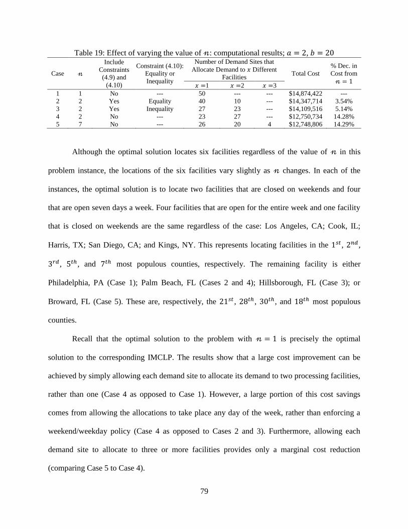
79
Table 19: Effect of varying the value of 𝓃: computational results; 𝑎 = 2, 𝑏 = 20
Case 𝓃
Include
Constraints
(4.9) and
(4.10)
Constraint (4.10):
Equality or
Inequality
Number of Demand Sites that
Allocate Demand to 𝑥 Different
Facilities Total Cost
% Dec. in
Cost from
𝓃 = 1 𝑥 =1 𝑥 =2 𝑥 =3
1 1 No --- 50 --- --- $14,874,422 ---
2 2 Yes Equality 40 10 --- $14,347,714 3.54%
3 2 Yes Inequality 27 23 --- $14,109,516 5.14%
4 2 No --- 23 27 --- $12,750,734 14.28%
5 7 No --- 26 20 4 $12,748,806 14.29%
Although the optimal solution locates six facilities regardless of the value of 𝓃 in this
problem instance, the locations of the six facilities vary slightly as 𝓃 changes. In each of the
instances, the optimal solution is to locate two facilities that are closed on weekends and four
that are open seven days a week. Four facilities that are open for the entire week and one facility
that is closed on weekends are the same regardless of the case: Los Angeles, CA; Cook, IL;
Harris, TX; San Diego, CA; and Kings, NY. This represents locating facilities in the 1𝑠𝑡, 2𝑛𝑑,
3𝑟𝑑, 5𝑡ℎ, and 7𝑡ℎ most populous counties, respectively. The remaining facility is either
Philadelphia, PA (Case 1); Palm Beach, FL (Cases 2 and 4); Hillsborough, FL (Case 3); or
Broward, FL (Case 5). These are, respectively, the 21𝑠𝑡 , 28𝑡ℎ, 30𝑡ℎ, and 18𝑡ℎ most populous
counties.
Recall that the optimal solution to the problem with 𝓃 = 1 is precisely the optimal
solution to the corresponding IMCLP. The results show that a large cost improvement can be
achieved by simply allowing each demand site to allocate its demand to two processing facilities,
rather than one (Case 4 as opposed to Case 1). However, a large portion of this cost savings
comes from allowing the allocations to take place any day of the week, rather than enforcing a
weekend/weekday policy (Case 4 as opposed to Cases 2 and 3). Furthermore, allowing each
demand site to allocate to three or more facilities provides only a marginal cost reduction
(comparing Case 5 to Case 4).

80
4.5.2 Restricting the Maximum Allowed Travel Time
The optimal solution to (2.4), (3.5), (3.7), (3.8) and (4.1) - (4.10) may be such that some
of the allocations assign a demand site 𝑖 ∈ 𝐼 to a facility 𝑗4 ∈ 𝐽 that is relatively close during the
week, but assign 𝑖 to another facility 𝑗5 ∈ 𝐽 that is very far away on weekends. Thus, we utilize
the constraints discussed in Section 4.4.3, to restrict the maximum allowed travel time. All of the
results presented to address this situation correspond to Case 3 of the cyclic allocation model
described in Table 18 and Table 19 (i.e., a weekday/weekend allocation policy given by (2.4),
(3.5), (3.7), (3.8) and (4.1) - (4.10) for 𝑛 = 2 when (4.10) is implemented as an inequality
constraint).
Maximum Travel Time Constraints
When there is no restriction on the maximum travel days (i.e., 𝑡𝑚𝑎𝑥 ≥ 𝑡∗), the optimal
allocation scheme is such that all demand sites are allocated to a processing facility that can be
reached within 22 days; no demand-facility allocation pair requires 𝑡∗ = 29 days of travel time
in the optimal solution. Further restricting the travel time to 11 days (a 50% reduction in
maximum travel days) results in only a 1.3% increase in cost and a 14% decrease in the demand-
weighted average travel time. As a result, the solution that results from restricting the maximum
travel time allowed to 11 days may be an attractive solution to facility managers who are
concerned with the amount of time demands are in transit. However, any further restrictions in
travel time come at a significant cost; restricting the maximum travel time to ten days results in a
6.3% increase in cost when compared to a maximum travel time of 11 days. The percent cost

81
increase due to restricting the maximum travel time can be seen graphically in Figure 14 and the
details are given in Table 20.
Figure 14: Cost effect of restricting travel time; max 7,...,29t days; 𝑎 = 2, 𝑏 = 20
Table 20: Effect of restricting travel time; 𝑎 = 2, 𝑏 = 20
𝑡𝑚𝑎𝑥
# of Demand
Sites
Allocated to a
Facility 𝑡𝑚𝑎𝑥
Days Away
% Increase
in Cost over
Unrestricted
Instance
# of
Facilities
Located
Cost Breakdown ($)
Total Cost
($) Location Transportation Backlog
1 50 293.71% 50 48,176,400 1,836,932 5,537,400 55,550,732
2 24 143.61% 28 27,193,300 2,499,820 4,678,560 34,371,680
3 16 82.96% 18 17,583,400 3,222,198 5,009,860 25,815,458
4 20 48.34% 13 12,801,800 4,161,860 3,966,660 20,930,320
5 9 25.38% 10 9,948,800 4,611,892 3,129,980 17,690,672
6 7 13.63% 8 8,052,000 5,182,334 2,797,640 16,031,974
7 3 10.16% 8 8,048,600 4,999,604 2,494,720 15,542,924
8 2 9.59% 8 8,043,200 5,221,784 2,198,140 15,463,124
9 7 8.52% 8 8,048,600 5,474,212 1,789,000 15,311,812
10 1 7.70% 8 8,048,600 5,520,664 1,627,140 15,196,404
11 5 1.31% 7 7,087,000 6,084,212 1,122,700 14,293,912
12 2 0.79% 7 7,087,000 5,992,454 1,141,260 14,220,714
13 1 0.61% 7 7,087,000 6,017,134 1,091,000 14,195,134
14 3 0.60% 6 6,128,000 6,544,686 1,521,580 14,194,266
15 1 0.55% 7 7,087,600 6,027,608 1,071,860 14,187,068
16 2 0.12% 7 7,087,600 5,980,494 1,057,800 14,125,894
17-19 0 0.12% 7 7,087,600 5,980,494 1,057,800 14,125,894
20 2 0.11% 6 6,128,000 6,685,510 1,311,540 14,125,050
21 0 0.11% 6 6,128,000 6,685,510 1,311,540 14,125,050
22 1 0.00% 6 6,135,500 6,562,816 1,411,200 14,109,516
23-29 0 0.00% 6 6,135,500 6,562,816 1,411,200 14,109,516
14
14.2
14.4
14.6
14.8
15
15.2
15.4
15.6
15.8
024681012141618202224262830
To
tal
Co
st (
in m
llio
ns)
Max Travel Days Allowed
Restrict Travel Time
1.3% Increase
in Cost
6.3% Increase
in Cost
More Restrictive

82
In general, as the value of maxt decreases, the number of facilities located, location costs,
and backlogging costs increase while the transportation costs decrease. We note that the table
indicates that certain values of maxt (e.g., max 13,14,15t ) do not follow this general pattern.
This is likely due to the particular demand instance used.
Additionally, we remind the reader that all demands must undergo one day of processing,
which is included in the transportation cost, regardless of whether or not the demands are
processed at the same location in which they originate. Thus, the transportation cost of
$1,836,932 when 𝑡𝑚𝑎𝑥 = 1 is precisely 𝑎 = 2 times the total number of demands generated
during the planning horizon (918,466). Figure 15 displays the effect of restricting the travel time
on the three cost components that comprise the objective function, as well as the optimal
objective function value.
Figure 15: Cost effect of restricting travel time; 𝑎 = 2, 𝑏 = 20
Since the solution to the 𝑡𝑚𝑎𝑥 = 11 constraint addition to Case 3 serves as a base case for
many of the following analyses due to the reasons outlined at the beginning of this section, we
display the corresponding optimal locations and arriving allocations in Figures 16-18. The
optimal solution locates facilities at Los, Angeles, CA; San Diego, CA; Harris, TX; Orange, FL;
0
10
20
30
40
50
60
0 5 10 15 20 25 30
Co
st (
in M
illi
ons)
Max Travel Days Allowed
Cost Effect of Restricting Travel Time
Total Cost
Transportation Cost
Location Cost
Inventory Cost

83
Cook, IL; Philadelphia, PA; and Queens, NY. The five most populous counties in the U.S. are
identified by a circle; a processing facility located in one of these counties will be open every
day of the week.
Figure 16: Optimal locations and allocations arriving on weekdays for Case 3; 𝑎 = 2, 𝑏 = 20,
max 11t
Figure 17: Optimal locations and allocations arriving on Saturdays for Case 3; 𝑎 = 2, 𝑏 = 20,
max 11t
One of the 5 most populous counties
Demand site
Located processing
facility
Noteworthy Sites Demands from this
demand site do not
arrive at any processing facility on
this day of the week
& the demand site is not also a processing
facility
Demands from this
demand site do not arrive at any
processing facility on
this day of the week & the demand site is
also a located
processing facility
One of the 5 most
populous counties
Demand site
Located processing facility
Noteworthy Sites
Demands from this
demand site do not arrive at any
processing facility on
this day of the week & the demand site is
not also a processing facility
Demands from this
demand site do not
arrive at any processing facility on
this day of the week
& the demand site is also a located
processing facility

84
Figure 18: Optimal locations and allocations arriving on Sundays for Case 3; 𝑎 = 2, 𝑏 = 20,
max 11t
We note that the figures display where demand that is arriving at a processing facility on
a particular day (i.e., weekday, Saturday, or Sunday) came from, rather than where the demand is
being shipped on a particular day. For example, a connection from the Salt Lake, UT demand
site to the San Diego, CA processing facility on Sunday’s map (i.e., Figure 18) indicates that Salt
Lake’s demands arrive at the San Diego facility on Sundays. Since it takes eight days for the
demand generated at Salt Lake to be ready for processing at San Diego, the demands must have
been shipped from Salt Lake on a Saturday.
On some days, no processing facility receives demands from a particular demand-
generating site. These demand sites are identified by triangles (if they are not also processing
facilities) or stars (if they are processing facilities) in Figure 17 and Figure 18. For example,
none of the processing facilities receive demands from Salt Lake, UT on Saturday; all of Salt
Lake’s demand arrives at processing facilities on either a weekday or on Sunday. This is
indicated by a triangle. Additionally, none of the processing facilities receive demands from the
One of the 5 most
populous counties
Demand site
Located processing facility
Noteworthy Sites
Demands from this
demand site do not arrive at any
processing facility on
this day of the week & the demand site is
not also a processing
facility
Demands from this demand site do not
arrive at any
processing facility on this day of the week
& the demand site is
also a located processing facility

85
demand sites located in Philadelphia, PA and Queens, NY, which are both also processing
facilities themselves. This is indicated by a star.
Many of the demand sites along the Atlantic coast do not allocate demands to arrive at
processing facilities on Saturdays. This is because there is no nearby processing facility that is
open on the weekends so it is cheaper to let the demands spend more time in transit and arrive at
a facility on Sunday. This way, the demands can either be processed on Sunday (if the facility is
open on weekends) or only have to incur one day (Sunday) of backlog cost rather than two
(Saturday and Sunday). Demand sites and processing facilities whose demand does arrive at a
processing facility on the day under consideration are denoted by a small square and a large
square, respectively.
An example of the optimal cyclic allocations is depicted in Table 21 for the Salt Lake,
UT demand site. Notice that demands leave the Salt Lake, UT demand site each day of the week,
but only arrive at processing facilities on Sunday through Friday due to the extended travel time
between Salt Lake, UT and San Diego, CA. This explains the triangle over Salt Lake, UT in
Figure 17.
Table 21: Cyclic allocations for Salt Lake, UT
Day of Week Demand
Leaves Salt Lake, UT
Processing Facility to
which Demand is
Allocated
Travel Time Between
Salt Lake, UT and
Processing Facility
Day of Week Demand
Arrives at Processing
Facility
Sunday Los Angeles, CA 7 Days Sunday
Monday Los Angeles, CA 7 Days Monday
Tuesday Los Angeles, CA 7 Days Tuesday
Wednesday Los Angeles, CA 7 Days Wednesday
Thursday Los Angeles, CA 7 Days Thursday
Friday Los Angeles, CA 7 Days Friday
Saturday San Diego, CA 8 Days Sunday

86
Restricting the Time Difference between Weekday and Weekend Allocations
While we can impose constraints (4.14) for any nonnegative integer value of 𝑚, the case
of 𝑚 = 2 is of particular interest since items that arrive at a facility that is closed on the
weekends must wait in backlog for two days before they can be processed. This allows us to use
the two days as (less-expensive) transportation days. Table 22 shows how varying the value of 𝑚
affects the total cost, cost breakdown, and number of facilities located for the 𝑡𝑚𝑎𝑥 = 11
restriction of Case 3. For all values of 𝑚, the model locates facilities in Cook, IL; Harris, TX;
Los Angeles, CA; and San Diego, CA, which are among the five most populous counties and
therefore are open seven days per week. In addition, all solutions locate a facility that is only
open on weekdays in Philadelphia, PA. When 𝑚 = 0, an additional weekday facility is located in
Kings, NY; however, it is replaced with a facility in Queens, NY when 𝑚 ≥ 1. Finally, a seventh
facility is located in Orange, FL when 𝑚 ≥ 7. The results show that allowing a slight increase in
the travel time between weekday and weekend allocations results in a cost decrease that is nearly
half the cost decrease that would be possible if the difference were unrestricted.
Table 22: Effect of restricting the time difference; 𝑎 = 2, 𝑏 = 20
𝑚 Total Cost
($)
% Increase in
Cost over
Unrestricted
Instance
# of
Facilities
Located
Cost Breakdown ($)
Location Transportation Backlog
0 14,773,536 3.35% 6 6,137,700 6,741,736 1,894,100
1-6 14,554,808 1.83% 6 6,135,600 6,771,708 1,647,500
7 14,373,362 0.56% 7 7,087,000 6,103,982 1,182,380
≥8 14,293,912 0.00% 7 7,087,000 6,084,212 1,122,700

87
Closest Assignment Constraints
In Table 23 we investigate the effect of allowing a demand site to be allocated to the
closest 𝜍 facilities with respect to the difference in travel time between weekday and weekend
assignments for the 𝑡𝑚𝑎𝑥 = 11 addition to Case 3. The optimal solution in each instance had at
least one assignment in which the travel time from a demand site to a processing facility was
𝑡𝑚𝑎𝑥 = 11 and, except for the instance with 𝜍 = 1, had a weekend assignment with an eight day
longer travel time than the weekday assignment. All of the instances located seven facilities (but
not necessarily the same facilities). Allowing demands to be assigned to the second closest
facility results in a significant cost savings compared to the case in which all demands must be
assigned to the closest located facility.
Table 23: Effect of imposing closest assignment constraints; 𝑎 = 2, 𝑏 = 20
𝜍 Total Cost
($)
% Increase in Cost over
Unrestricted Instance
Cost Breakdown ($) Facilities Located
(Node #) Location Transportation Backlog
1 15,950,538 11.59% 7,094,900 6,222,878 2,632,760 1, 2, 3, 5, 7, 14, 21
2 14,675,446 2.67% 7,082,200 5,723,666 1,869,580 1, 2, 3, 5, 21, 23, 30
3,4 14,343,048 0.34% 7,087,000 5,992,148 1,263,900 1, 2, 3, 5, 10, 21, 35
≥5 14,293,912 0.00% 7,087,000 6,084,212 1,122,700 1, 2, 3, 5, 10, 21, 35
4.5.3 Allocation Composition
To understand how many demand sites take advantage of the ability to allocate their
demand to more than one processing facility, we graph the number of demand sites that adhere to
each allocation method possible in Case 3 as described in Table 18, with the added 𝑡𝑚𝑎𝑥 = 11
restriction. In particular, Figure 19 and Figure 20 display the number of demand sites that
1) only allocate demand to one processing facility;

88
2) allocate demand to two processing facilities, with demand arriving at a different facility
on Saturday than Sunday; and
3) allocate demand to two processing facilities, with demand arriving at the same facility on
Saturday and Sunday
as the cost of holding items in backlog varies.
Demand sites that allocate according to the second or third method utilize the flexibility
provided by cyclic allocations. Thus, we quantify the diversity of demand allocations by giving
each instance an allocation score that accounts for the number of demand sites that are assigned
to each of the three possible allocation methods. Demand sites contribute a value of 1, 2, or 3,
depending on whether they allocate demand according to the first, second, or third method,
respectively. For example, an allocation score of 67 is given to the optimal solution when 𝑏 = 10
since it assigns 36 demand sites to only one processing facility, 11 to two processing facilities
with demand arriving at a different facility on Saturday than Sunday, and 3 to two processing
facilities with demand arriving at the same facility on Saturday and Sunday (i.e., 36 ∗ 1 + 11 ∗
2 + 3 ∗ 3 = 67). Since there are 50 demand sites, the lowest possible allocation score is 50 and
corresponds to a solution that is no different from what would be obtained using the original
IMCLP model (i.e., all demand sites are assigned to only one processing facility). The highest
possible allocation score is 150, though the highest realized score in Figure 19 is only 72.
89
Figure 19: Types of allocations in the optimal solution as the backlog cost varies; 𝑎 = 2
Figure 20: Types of allocations in the optimal solution as the backlog cost varies; 𝑎 = 2
The allocation score generally increases as the backlog cost increases when six facilities
are located. However, the allocation score remains relatively constant for 𝑏 values that locate
seven facilities in the optimal solution. Furthermore, the optimal solution to the 𝑏 ≥ 15 instances
displayed in Figures 19 and 20 assigns approximately 30 demand sites to only one processing
facility and 20 demand sites to two processing facilities, with demand arriving at a different
processing facility on Saturday than Sunday; in this case, the allocation for six days (weekdays
and one weekend day) is the same.
0
10
20
30
40
50
60
70
80
90
100
0
10
20
30
40
50
60
70
80
90
100
1 2 3 4 5 6 7 8 9 10 11 12 13 14 15 16 17 18 19 20
All
oca
tion S
core
All
oca
tio
n C
om
po
siti
on:
Num
ber
of
Dea
man
d S
ites
Backlog Cost (b)
2 Allocations, Sat & Sun Same
2 Allocations, Sat & Sun Different
1 Allocation
Allocation Score
0
10
20
30
40
50
60
70
80
90
100
0
10
20
30
40
50
60
70
80
90
100
10 20 30 40 50 60 70 80 90 100
All
oca
tion S
core
All
oca
tio
n C
om
po
siti
on:
Num
ber
of
Dea
man
d S
ites
Backlog Cost (b)
2 Allocations, Sat & Sun Same
2 Allocations, Sat & Sun Different
1 Allocation
Allocation Score
# Located 6 7
Facilities Facilities
# Located 6 Facilities 7 Facilities

90
We further quantify the difference between the optimal cyclic solution and the optimal
IMCLP solution by comparing their costs in Figure 21. The figure shows that the flexibility
allowed by cyclic allocations results in increased cost savings as the cost of holding backlogged
items increases. In particular, the cyclic allocations result in a 3.9% decrease in cost in our base
case instance (i.e., 𝑏 = 20) when compared to the corresponding optimal IMCLP solution. If the
backlog cost were doubled (i.e., 𝑏 = 40) we would see a 7.85% decrease in cost. At a backlog
cost of 𝑏 = 100, an 11.27% decrease in cost is achieved.
Figure 21: % decrease in cost obtained by using the cyclic allocation model as compared to the
IMCLP model; 𝑎 = 2
4.5.4 Solution Robustness
In facility location modeling it is extremely important to correctly identify which
processing facilities to locate, since it is often very difficult and costly to change the locations
once they are established. While it is also important to correctly identify the allocations, these
can be adapted more easily than the locations. This motivates our desire to determine how robust
the optimal solution is to the particular demand instance used.
To test the solution robustness, we consider ten demand instances. In each of these
instances, Case 3 with the added 𝑡𝑚𝑎𝑥 = 11 restriction is used. We first solve Instance 1 to
0%
2%
4%
6%
8%
10%
12%
0 20 40 60 80 100
% D
ecre
ase
i n C
ost
Backlog cost (b)
Cost Benefit of using Cyclic Assignments

91
optimality and then compare the solution to those of the remaining instances under the following
three conditions:
(1) forcing the Instance 1 allocations and locations into the remaining instances,
(2) forcing only the Instance 1 locations into the remaining instances, and
(3) solving the remaining instances to optimality without considering the Instance 1
solution.
The results indicated that each of the ten instances (under condition (3)) identified the
same seven processing facilities to locate in the optimal solution. Although the optimal
allocations differed slightly among the instances, these variations always resulted in less than a
0.1% increase in total cost when the Instance 1 optimal locations and allocations were imposed
on the other instances (i.e., scenario (1)); the average increase in cost was 0.028%. This is
particularly noteworthy since the transportation and backlogging costs are intimately linked to
the allocation decisions and account for roughly 50% of the total cost. The details are displayed
in Table 24.
Table 24: % Increase in Cost from using the Optimal Locations and Allocations of Instance 1
instead of the Optimal Solution for the Particular Instance; 𝑎 = 2, 𝑏 = 20
Instance Total Location Transportation Backlog
1 0.000% 0.000% 0.000% 0.000%
2 0.001% 0.000% -0.025% 0.198%
3 0.060% 0.000% -0.147% 1.564%
4 0.022% 0.000% -0.646% 4.021%
5 0.055% 0.000% -0.569% 4.008%
6 0.029% 0.000% -0.543% 3.449%
7 0.008% 0.000% -0.637% 3.721%
8 0.000% 0.000% 0.000% 0.000%
9 0.054% 0.000% -0.636% 4.451%
10 0.052% 0.000% -0.210% 1.870%
Average 0.028% 0.000% -0.341% 2.328%

92
4.6 Chapter Summary
We introduced a variant of the IMCLP that allows for a cyclic allocation approach to
assigning demand sites to processing facilities. This enables the model to develop a day-of-the-
week allocation policy that considers deterministic fluctuations in the daily processing capacity
levels of the facilities or stochastic fluctuations in the average demand by day-of-the-week. For
example, our model is able to adjust the allocation policy to account for some facilities being
closed on weekends. In the spirit of the IMCLP model developed in Chapter 3, the model
presented in this chapter also allows disaggregated daily demand parameters to serve as inputs
directly into the model and mitigates the hard capacity constraints that are typically found in
capacitated facility location models by allowing unprocessed demand to be held in backlog and
processed at a later date. Through computational studies, we showed that incorporating this
cyclic allocation approach into the model can result in a significant cost savings as compared to
models that do not incorporate this approach, such as the IMCLP. Furthermore, we note that the
model can readily be restructured to deal with other cycles, such as annual cycles with demand
assignments that either change seasonally or monthly in response to time-varying demand
patterns.
We also presented multiple constraints that can be added to the model formulation to
achieve various operational goals. These include (1) restricting the number of processing
facilities to which a demand site can be assigned, (2) introducing a weekday/weekend allocation
policy, and (3) bounding the difference between the travel time of a weekday assignment and a
weekend assignment. Our results suggest that a significant cost reduction can be achieved by
implementing the cyclic allocation model as compared to capacitated facility location models

93
that require a static allocation policy. Much of this benefit can be achieved even when additional
constraints of the form outlined above are imposed.

94
CHAPTER 5: Chance Constrained IMCLP with Uncertain Demand
5.1 Motivation
In reality, a facility manager faces many sources of operational uncertainty, including
uncertainty related to demand, machine processing capacity, personnel availability,
purchasing/selling prices, and shipment travel times. The many sources of uncertainty make it
impossible to model all of the uncertainty simultaneously due to the resulting model
intractability, computational limitations, or data requirements. Thus, in this chapter, we focus
solely on stochasticity that arises in demand.
We note that while the deterministic IMCLP incorporates daily fluctuations in demand
over an extended time horizon, it is not explicitly formulated as a stochastic optimization
problem. Thus, in this chapter, we introduce a stochastic variant of the IMCLP with uncertain
demand. In addition to assessing a penalty cost associated with each day an item spends in
backlog (as is done in the IMCLP and cyclic allocation model), we use three different types of
chance constraints to restrict the number of demands that are backlogged to a predetermined
threshold. The first approach incorporates joint chance constraints that ensure the probability of
any processing facility having a backlog level above the threshold on any day of the planning
horizon is sufficiently small. We also model individual chance constraints on the amount of
backlog at each facility each day, as well as a hybrid approach which accounts for the probability
that each individual processing facility will exceed the stated maximum backlog level on any day
of the planning horizon. We then present mixed-integer programming reformulations of the

95
chance constraints that incorporate a finite number of scenarios from a given known demand
distribution. (We refer the interested reader to Birge and Louveaux (2011) for an introduction to
chance constraints.)
The resulting models are solved using two different decomposition schemes and their
performance is compared to that of a generic solver. The first decomposes the problem into two
stages: the long-term (i.e., location and allocation) decisions are determined in the first stage
while the daily (i.e., processing and backlog) decisions are determined in the second stage.
Benders decomposition is used to solve the resulting formulation. The second decomposition
scheme capitalizes on the problem structure by utilizing a three-stage approach. In particular,
given a feasible first-stage location and allocation solution, we can readily determine the optimal
second-stage processing and backlog decisions as well as the third-stage auxiliary variables that
verify whether the chance constraints are satisfied by inspection. If the chance constraints are
violated, a corresponding cut is added to the first-stage problem.
5.2 Joint Chance Constrained Formulation
As mentioned, we will incorporate three types of chance constraints into the stochastic
IMCLP: joint chance constraints, individual chance constraints, and a hybrid approach. The
majority of this chapter will focus on the joint chance constrained model, which we formulate in
this section. The individual chance constraints and the hybrid approach will be introduced in
Section 5.4.
In each of the formulations, we incorporate demand stochasticity into the IMCLP using a
scenario based approach in which a scenario corresponds to a realization of the daily demand for
every day within the time horizon. For example, if the time horizon is one year, the demand

96
generated on each day of the year at each demand site is collectively referred to as a scenario.
We let Ω represent the set of all possible demand scenarios, and 𝑝𝜔 represent the probability of a
particular scenario 𝜔 ∈ Ω. It is assumed that ∑ 𝑝𝜔𝜔∈Ω = 1. Additionally, the parameter ℎ𝑖𝑑
corresponds to the random daily demand generated at demand point 𝑖 ∈ 𝐼 on day 𝑑 ∈ 𝐷. While
ℎ𝑖𝑑 is a random parameter, ℎ𝑖𝑑𝜔 represents a realization of the random demand ℎ𝑖𝑑 in scenario
𝜔 ∈ Ω generated at 𝑖 ∈ 𝐼 on day 𝑑 ∈ 𝐷 and 𝜉(𝜔) ∈ ℕ0|𝐼|×|𝐷|
is a vector containing the demand
realizations ℎ𝑖𝑑𝜔 , ∀𝑖 ∈ 𝐼, 𝑑 ∈ 𝐷 corresponding to scenario 𝜔 ∈ Ω.
Since we assume that the facility location and assignment decisions must remain constant
throughout the planning horizon, variables 𝑋𝑗 and 𝑌𝑖𝑗, which represent these decisions, are
scenario independent in the stochastic IMCLP. For fixed location and allocation decisions, the
processing and backlog variables become apparent once the scenario is observed. Thus, we let
𝑊𝑗𝑑𝜔 and 𝑉𝑗𝑑
𝜔 be the corresponding scenario dependent variables (or equivalently, recourse
variables). In summary, the decision variables for the IMCLP model with stochastic demand are:
Decision Variables
𝑋𝑗 = 1
0
If we locate at facility 𝑗 ∈ 𝐽
Otherwise
𝑌𝑖𝑗 = 1
0
If we assign demand site 𝑖 ∈ 𝐼 to facility 𝑗 ∈ 𝐽
Otherwise
𝑉𝑗𝑑𝜔 Backlog at site 𝑗 ∈ 𝐽 at the beginning of day 𝑑 ∈ 𝑡∗ + 1,… , |𝐷| + 1 in scenario 𝜔 ∈ Ω
𝑊𝑗𝑑𝜔 Number of items processed at site 𝑗 ∈ 𝐽 on day 𝑑 ∈ 𝑡∗ + 1,… , |𝐷| in scenario 𝜔 ∈ Ω
The specific aim of incorporating the joint chance constraint into the stochastic IMCLP is
to minimize the total facility, expected transportation, and expected backlogging costs, while

97
ensuring the probability that the backlog at any facility never exceeds a predetermined level of 𝜃
is bounded from below by a given reliability level 1 − 𝜏. The joint chance constraint is
ℙ(𝑗𝑑 ≤ 𝜃; ∀𝑗 ∈ 𝐽, 𝑑 ∈ 𝑡∗ + 1,… , |𝐷| + 1) ≥ 1 − 𝜏 (5.1)
where ℙ(⋅) denotes the probability of event ⋅ occurring and 𝑗𝑑 represents the stochastic
counterpart of the random outcome 𝑉𝑗𝑑𝜔, ∀𝜔 ∈ Ω.
5.2.1 Single Stage Formulation with Probabilistic Constraint
With this additional notation, the joint chance constrained IMCLP with stochastic
demands is formulated as follows:
[JCC]:
𝑀𝑖𝑛𝑿,𝒀,𝑽,𝑾 (|𝐷| − 𝑡∗)∑ 𝑓𝑗𝑋𝑗𝑗∈𝐽 + 𝑎∑ ∑ ∑ 𝔼𝜉[ℎ𝑖𝑑]𝑡𝑖𝑗𝑌𝑖𝑗𝑗∈𝐽
|𝐷|𝑑=𝑡∗+1𝑖∈𝐼
+𝑏 𝔼𝜉[∑ ∑ 𝑗𝑑𝑗∈𝐽|𝐷|+1𝑑=𝑡∗+2 ] (5.2)
Subject to
∑ 𝑌𝑖𝑗𝑗∈𝐽 = 1 ∀𝑖 ∈ 𝐼 (2.2)
𝑌𝑖𝑗 ≤ 𝑋𝑗 ∀𝑖 ∈ 𝐼; 𝑗 ∈ 𝐽 (2.3)
ℙ(𝑗𝑑 ≤ 𝜃; ∀𝑗 ∈ 𝐽, 𝑑 ∈ 𝑡∗ + 1,… , |𝐷| + 1) ≥ 1 − 𝜏 (5.1)
𝑉𝑗,𝑑+1𝜔 − 𝑉𝑗𝑑
𝜔 +𝑊𝑗𝑑𝜔 = ∑ ℎ𝑖,𝑑−𝑡𝑖𝑗
𝜔 𝑌𝑖𝑗𝑖∈𝐼 ∀𝑗 ∈ 𝐽; 𝑑 ∈ 𝑡∗ + 1,… , |𝐷|; 𝜔 ∈ Ω (5.3)
𝑊𝑗𝑑𝜔 ≤ 𝑘𝑗𝑋𝑗 ∀𝑗 ∈ 𝐽; 𝑑 ∈ 𝑡∗ + 1,… , |𝐷|; 𝜔 ∈ Ω (5.4)
𝑉𝑗,𝑡∗+1𝜔 = 𝑣𝑗𝑋𝑗 ∀𝑗 ∈ 𝐽; 𝜔 ∈ Ω (5.5)
𝑉𝑗𝑑𝜔 ≥ 0 ∀𝑗 ∈ 𝐽; 𝑑 ∈ 𝑡∗ + 1,… , |𝐷| + 1; 𝜔 ∈ Ω (5.6)
𝑊𝑗𝑑𝜔 ≥ 0 ∀𝑗 ∈ 𝐽; 𝑑 ∈ 𝑡∗ + 1,… , |𝐷|; 𝜔 ∈ Ω (5.7)

98
𝑋𝑗 ∈ 0,1 ∀𝑗 ∈ 𝐽 (2.4)
𝑌𝑖𝑗 ∈ 0,1 ∀𝑖 ∈ 𝐼; 𝑗 ∈ 𝐽 (3.6)
Where
𝔼𝜉[ℎ𝑖𝑑] = ∑ 𝑝𝜔ℎ𝑖𝑑𝜔
𝜔∈Ω (5.8)
and
𝔼𝜉[∑ ∑ 𝑗𝑑𝑗∈𝐽|𝐷|+1𝑑=𝑡∗+2 ] = ∑ 𝑝𝜔 ∑ ∑ 𝑉𝑗𝑑
𝜔𝑗∈𝐽
|𝐷|+1𝑑=𝑡∗+2𝜔∈Ω . (5.9)
The objective function (5.2) minimizes the facility location costs, as well as the expected
transportation and backlogging costs over the entire time horizon (i.e., days 𝑡∗ + 1 to |𝐷|). We
note that the expected backlog at the beginning of day |𝐷| + 1 is precisely the amount of backlog
at the end of day |𝐷|, and as such, including this term in the objective function allows the model
to capture the backlog level at the end of the planning horizon.
Although the backlog levels will be determined to meet the desired service levels
specified in the joint chance constraint (5.1) our objective function also explicitly captures the
backlogging costs. This allows the model to differentiate between solutions that contain different
amounts of backlog. For example, our formulation would give preference to a solution in which
no items are held in backlog over a solution that meets the service level requirements but holds 𝜃
items in backlog at each facility every day, given that the two solutions have the same location
and allocation cost.
As before, constraints (2.2) and (3.6) enforce single sourcing constraints on the demand
sites while constraints (2.3) ensure demand sites are only assigned to located facilities.
Constraint (5.1) is the joint chance constraint that ensures the probability that the backlog at any
facility never exceeds a predetermined level of 𝜃 is bounded from below by a given reliability
level 1 − 𝜏. Constraints (5.3) are flow balance constraints to update the amount of demand held

99
in backlog from day to day. They also serve, along with constraints (5.4), as capacity constraints.
Specifically, constraints (5.3) ensure the amount of demand processed each day does not exceed
the amount available for processing while constraints (5.4) limit the maximum amount of
demand processed each day to the daily processing capacities of the facilities. Constraints (5.5)
state that a located facility 𝑗 ∈ 𝐽 will have an initial backlog of 𝑣𝑗 and a facility that is not located
will have an initial backlog level of zero. Constraints (2.4), (3.6), (5.6), and (5.7) are standard
non-negativity and binary constraints.
5.2.2 MIP Reformulation
Since formulation JCC is nonlinear due to the joint chance constraint (5.1), we present a
mixed integer linear reformulation that approximates JCC by using a finite subset Ω′ ⊆ Ω of all
possible demand scenarios. Furthermore, we let 𝜔′ ∈ Ω′ deonote elements of Ω′ and define ℎ𝑖𝑑𝜔′,
𝑉𝑗𝑑𝜔′, 𝑊𝑗𝑑
𝜔′, 𝜉(𝜔′), and 𝑝𝜔′accordingly (with ∑ 𝑝𝜔
′ 𝜔′∈Ω′ = 1 and 𝜉(𝜔′) often referred to as 𝜉′ for
readability. With this notation, we introduce decision variables
𝑍𝜔′=
1
0
If the backlog at any facility exceeds θ on any day in scenario ω′ ∈ Ω′
Otherwise
and replace (5.1) with
𝑉𝑗𝑑𝜔′ −𝑀1𝑍
𝜔′ ≤ 𝜃 ∀ 𝑗 ∈ 𝐽; 𝑑 ∈ 𝑡∗ + 1,… , |𝐷| + 1; 𝜔′ ∈ Ω′ (5.10)
∑ 𝑝𝜔′𝑍𝜔′
𝜔′∈Ω′ ≤ 𝜏 (5.11)
𝑍𝜔′∈ 0,1 ∀𝜔′ ∈ Ω′ (5.12)
Constraints (5.10) define the binary service level variables where 𝑀1 is a sufficiently large
number such that the constraint is satisfied by letting 𝑍𝜔′= 1 when 𝑉𝑗𝑑
𝜔′ > 𝜃 for some facility 𝑗

100
on some day 𝑑 in some scenario 𝜔′ ∈ Ω′. Constraint (5.11) guarantees that the probability of
violating the joint chance constraint is no more than 𝜏. Note that we can write constraint (5.11) as
∑ 𝑍𝜔′
𝜔′∈Ω′ ≤ ⌊𝜏|Ω′|⌋ (5.13)
if each scenario 𝜔′ ∈ Ω′ occurs with equal probability. Finally, constraints (5.12) are standard
binary constraints. This results in the following mixed integer linear reformulation of JCC:
[MIP-JCC]:
= 𝑀𝑖𝑛𝑿,𝒀,𝑽,𝑾,𝒁 (|𝐷| − 𝑡∗)∑ 𝑓𝑗𝑋𝑗𝑗∈𝐽 + 𝑎∑ ∑ ∑ 𝔼𝜉′[ℎ𝑖𝑑]𝑡𝑖𝑗𝑌𝑖𝑗𝑗∈𝐽
|𝐷|𝑑=𝑡∗+1𝑖∈𝐼
+𝑏 𝔼𝜉′[∑ ∑ 𝑗𝑑𝑗∈𝐽|𝐷|+1𝑑=𝑡∗+2 ] (5.14)
Subject to
∑ 𝑌𝑖𝑗𝑗∈𝐽 = 1 ∀𝑖 ∈ 𝐼 (2.2)
𝑌𝑖𝑗 ≤ 𝑋𝑗 ∀𝑖 ∈ 𝐼; 𝑗 ∈ 𝐽 (2.3)
𝑉𝑗𝑑𝜔′ −𝑀1𝑍
𝜔′ ≤ 𝜃 ∀𝑗 ∈ 𝐽; 𝑑 ∈ 𝑡∗ + 1,… , |𝐷| + 1; 𝜔′ ∈ Ω′ (5.10)
∑ 𝑝𝜔′𝑍𝜔′
𝜔′∈Ω′ ≤ 𝜏 (5.11)
𝑉𝑗,𝑑+1𝜔′ − 𝑉𝑗𝑑
𝜔′ +𝑊𝑗𝑑𝜔′ = ∑ ℎ𝑖,𝑑−𝑡𝑖𝑗
𝜔′ 𝑌𝑖𝑗𝑖∈𝐼 ∀𝑗 ∈ 𝐽; 𝑑 ∈ 𝑡∗ + 1,… , |𝐷|; 𝜔′ ∈ Ω′ (5.15)
𝑊𝑗𝑑𝜔′ ≤ 𝑘𝑗𝑋𝑗 ∀𝑗 ∈ 𝐽; 𝑑 ∈ 𝑡∗ + 1,… , |𝐷|; 𝜔′ ∈ Ω′ (5.16)
𝑉𝑗,𝑡∗+1𝜔′ = 𝑣𝑗𝑋𝑗 ∀𝑗 ∈ 𝐽; 𝜔′ ∈ Ω′ (5.17)
𝑉𝑗𝑑𝜔′ ≥ 0 ∀𝑗 ∈ 𝐽; 𝑑 ∈ 𝑡∗ + 1,… , |𝐷| + 1; 𝜔′ ∈ Ω′ (5.18)
𝑊𝑗𝑑𝜔′ ≥ 0 ∀𝑗 ∈ 𝐽; 𝑑 ∈ 𝑡∗ + 1,… , |𝐷|; 𝜔′ ∈ Ω′ (5.19)
𝑋𝑗 ∈ 0,1 ∀𝑗 ∈ 𝐽 (2.4)
𝑌𝑖𝑗 ∈ 0,1 ∀𝑖 ∈ 𝐼; 𝑗 ∈ 𝐽 (3.6)
𝑍𝜔′∈ 0,1 ∀𝜔′ ∈ Ω′ (5.12)

101
Where
𝔼𝜉′[ℎ𝑖𝑑] = ∑ 𝑝𝜔′ℎ𝑖𝑑𝜔′
𝜔′ ∈Ω′ (5.20)
and
𝔼𝜉′[∑ ∑ 𝑗𝑑𝑗∈𝐽|𝐷|+1𝑑=𝑡∗+2 ] = ∑ 𝑝𝜔
′∑ ∑ 𝑉𝑗𝑑
𝜔′𝑗∈𝐽
|𝐷|+1𝑑=𝑡∗+2𝜔′∈Ω′ . (5.21)
5.3 Solution Methods
As is evidenced in Section 5.5.2, solving problem instances with even a small number of
scenarios takes an exorbitant amount of time without employing any specialized solution
techniques. Therefore, in this section, we propose two-stage and three-stage decomposition
schemes to solve the mixed-integer programming reformulation of the joint chance-constrained
program with cutting-plane algorithms. As a means of identifying the decomposed problems, we
will use a labeling scheme of the form M#S# to identify the method and the problem stage. For
example, M1S2 refers to the second stage problem of the first decomposition scheme, whereas
M2S3 refers to the third stage problem of the second decomposition scheme.
5.3.1 Two-Stage Benders Decomposition Approach
The Benders decomposition [Benders, 1962] approach is one of the most effective
techniques for solving large-scale linear programming and mixed-integer programming models
that exhibit decomposable structures. The approach specifies two sets of variables, initial
decision variables and continuous recourse variables. At each iteration, the algorithm solves a
relaxed master problem at the first stage and passes a fixed first-stage optimal decision to the
second stage where recourse decisions are optimal for individual scenarios. Duality theorems are
then used to derive feasibility and optimality cuts, which affect the first-stage solution in

102
subsequent iterations. The algorithm terminates when all optimality conditions are satisfied and
no additional cuts are generated. We refer the interested reader to Birge and Louveaux (2011) for
a more detailed description of the decomposition technique.
Since Benders first introduced his decomposition scheme in 1962 in the context of
solving a general linear program, significant research has emerged that addresses algorithmic
improvements and modifications to accelerate the convergence of Benders decomposition
method as applied to facility location problems. Balinski and Wolfe (1963), Davis and Ray
(1969), and Geoffrion and Graves (1974) are among the earliest papers that apply Benders
decomposition to a facility location problem. Magnanti and Wong (1981) address the choice of
effective optimality cuts and have shown that the use of stronger cuts can reduce the number of
iterations, thereby improving the convergence of the algorithm. Wentges (1996) proposes a
procedure specifically for strengthening Benders cuts in the context of the capacitated facility
location problem. A review by Magnanti and Wong (1990) presents an overview of
decomposition methods for facility location problems. The review specifically addresses
methods of accelerating Benders decomposition and model selection criterion for facility
location problems.
In this section we develop a two-stage cutting plane algorithm based on the Benders
decomposition scheme to solve MIP-JCC. We place the long term decisions (i.e., location,
allocation) in the first stage and the daily decisions (i.e., processing, backlog) in the second stage.
For simplicity, we will denote ordered sets of variables using bold face type in the following
manner:1
1 We note that additional similar sets are created for variables introduced later in the chapter. For readability, we
adopt the convention that boldface type indicates such vectors and matrices, but we do not define every set in the
text. Instead, a detailed description of each ordered set can be found in the LIST OF SYMBOLS beginning on page
xvi.

103
𝑿: a 1 × |𝐽| vector whose 𝑗th element is 𝑋𝑗
𝒀: a |𝐼| × |𝐽| matrix whose (𝑖, 𝑗)th entry is 𝑌𝑖𝑗
𝑽𝝎′𝒋: a 1 × (|𝐷| + 1 − 𝑡∗) vector whose (𝑑 − 𝑡∗)th
element is 𝑉𝑗𝑑𝜔′
𝑽: a |𝐽| × (|𝐷| + 1 − 𝑡∗) × |Ω′| matrix whose (𝑗, 𝑑 − 𝑡∗, 𝜔)th element is 𝑉𝑗𝑑
𝜔′
𝑾𝝎′𝒋: a 1 × (|𝐷| − 𝑡∗) matrix whose (𝑑 − 𝑡∗)th element is 𝑊𝑗𝑑
𝜔′
𝑾: a |𝐽| × (|𝐷| − 𝑡∗) × |Ω′| matrix whose (𝑗, 𝑑 − 𝑡∗, 𝜔′)th element is 𝑊𝑗𝑑
𝜔′
𝒁: a 1 × |Ω| vector whose 𝜔′th element is 𝑍𝜔′
At the first stage we keep binary variables 𝑿, 𝒀, and 𝒁, and constraints (2.2), (2.3), and
(5.11). Without loss of generality, we add the constraint
∑ 𝑋𝑗𝑗∈𝐽 ≥ 1 (5.22)
to ensure at least one facility is located (this will become useful in the solution algorithms).
Alternatively, we could add the more restrictive constraint
∑ 𝑘𝑗𝑋𝑗𝑗∈𝐽 ≥∑ ∑ 𝔼
𝜉′[ℎ𝑖𝑑]
|𝐷|𝑑=𝑡+1𝑖∈𝐼
|𝐷|−𝑡∗ (5.23)
in place of constraint (5.22) to ensure that the cumulative capacity of the located facilities is
sufficient to handle the expected cumulative demand. We consider the relaxed master problem
as:
[M1S1]:
𝑀𝑖𝑛𝑿,𝒀,𝒁 (|𝐷| − 𝑡∗)∑ (𝑓𝑗𝑋𝑗 + 𝑎∑ ∑ 𝔼𝜉′[ℎ𝑖𝑑]
|𝐷|𝑑=𝑡∗+1𝑖∈𝐼 𝑡𝑖𝑗𝑌𝑖𝑗 + ∑ 𝑝𝜔
′𝜔
′𝑗(𝑿, 𝒀, 𝒁)𝜔′∈Ω′ )𝑗∈𝐽 (5.24)
Subject to
∑ 𝑌𝑖𝑗𝑗∈𝐽 = 1 ∀𝑖 ∈ 𝐼 (2.2)
𝑌𝑖𝑗 − 𝑋𝑗 ≤ 0 ∀𝑖 ∈ 𝐼; 𝑗 ∈ 𝐽 (2.3)

104
∑ 𝑋𝑗𝑗∈𝐽 ≥ 1 (5.22)
∑ 𝑝𝜔′𝑍𝜔
′
𝜔′∈Ω′ ≤ 𝜏 (5.11)
𝑋𝑗 ∈ 0,1 ∀𝑗 ∈ 𝐽 (2.4)
𝑌𝑖𝑗 ∈ 0,1 ∀𝑖 ∈ 𝐼; 𝑗 ∈ 𝐽 (3.6)
𝑍𝜔 ∈ 0,1 ∀𝜔 ∈ Ω (5.12)
where for each scenario 𝜔′ ∈ Ω′ and facility 𝑗 ∈ 𝐽, we optimize the following subproblem:
[M1S2(𝜔′, 𝑗)]:
𝜔′𝑗(𝑿, 𝒀, 𝒁) = 𝑀𝑖𝑛 𝑽𝝎′ 𝒋,𝑾𝜔′𝑗 ∑ 𝑉𝑗𝑑
𝜔′|𝐷|+1𝑑=𝑡∗+2 (5.25)
Subject to
𝑉𝑗,𝑑+1𝜔′ − 𝑉𝑗𝑑
𝜔′ +𝑊𝑗𝑑𝜔′ = ∑ ℎ𝑖,𝑑−𝑡𝑖𝑗
𝜔′ 𝑌𝑖𝑗𝑖∈𝐼 ∀𝑑 ∈ 𝑡∗ + 1,… , |𝐷| (5.26)
𝑊𝑗𝑑𝜔′ ≤ 𝑘𝑗𝑋𝑗 ∀𝑑 ∈ 𝑡∗ + 1,… , |𝐷| (5.27)
𝑉𝑗,𝑡∗+1𝜔′ = 𝑣𝑗𝑋𝑗 (5.28)
𝑉𝑗𝑑𝜔′ ≤ 𝜃 +𝑀1𝑍
𝜔 ∀𝑑 ∈ 𝑡∗ + 1,… , |𝐷| + 1 (5.29)
𝑉𝑗𝑑𝜔′ ≥ 0 ∀𝑑 ∈ 𝑡∗ + 1,… , |𝐷| + 1 (5.30)
𝑊𝑗𝑑𝜔′ ≥ 0 ∀𝑑 ∈ 𝑡∗ + 1,… , |𝐷| (5.31)
We associate dual variables 𝛾𝑑𝜔′𝑗, 𝜋𝑑
𝜔′𝑗, 𝜂
𝜔′𝑗, and 𝜇𝑑𝜔′𝑗
with constraints (5.26), (5.27),
(5.28), and (5.29), respectively. For each 𝜔′ ∈ Ω′ and 𝑗 ∈ 𝐽, the dual of M1S2(𝜔′, 𝑗) is:
[D-M1S2(𝜔′, 𝑗)]:
𝐷𝑢𝑎𝑙𝜔′𝑗 (𝑿, 𝒀, 𝒁) = 𝑀𝑎𝑥
𝜸𝝎′𝒋,𝝅𝝎
′𝒋,𝜂𝜔′𝑗,𝝁𝝎
′𝒋 ∑ ∑ ℎ𝑖,𝑑−𝑡𝑖𝑗
𝜔′ 𝑌𝑖𝑗𝛾𝑑𝜔′𝑗
𝑖∈𝐼|𝐷|𝑑=𝑡∗+1 + ∑ 𝑘𝑗𝑋𝑗𝜋𝑑
𝜔′𝑗|𝐷|𝑑=𝑡∗+1
+𝑣𝑗𝑋𝑗𝜂 𝜔′𝑗 + ∑ (𝜃 +𝑀1𝑍
𝜔′)𝜇𝑑𝜔′𝑗|𝐷|+1
𝑑=𝑡∗+1 (5.32)

105
Subject to
𝛾𝑑𝜔′𝑗
+ 𝜋𝑑𝜔′𝑗
≤ 0 ∀𝑑 ∈ 𝑡∗ + 1,… , |𝐷| (5.33)
𝜂 𝜔′𝑗 − 𝛾𝑡∗+1
𝜔′𝑗+ 𝜇𝑡∗+1
𝜔′𝑗≤ 0 (5.34)
𝛾𝑑−1𝜔′𝑗
− 𝛾𝑑𝜔′𝑗
+ 𝜇𝑑𝜔′𝑗
≤ 1 ∀𝑑 ∈ 𝑡∗ + 2,… , |𝐷| (5.35)
𝛾|𝐷|𝜔′𝑗
+ 𝜇|𝐷|+1𝜔′𝑗
≤ 1 (5.36)
𝜋𝑑𝜔′𝑗
≤ 0 ∀𝑑 ∈ 𝑡∗ + 1,… , |𝐷| (5.37)
𝜇𝑑𝜔′𝑗
≤ 0 ∀𝑑 ∈ 𝑡∗ + 1,… , |𝐷| + 1 (5.38)
Constraints (5.33) correspond to primal variables 𝑾𝜔′𝑗. Constraints (5.34) correspond to
the primal initial backlog variables, 𝑉𝑗,𝑡∗+1𝜔′ , constraints (5.35) correspond to primal variables
𝑉𝑗𝑑𝜔′ for 𝑑 ∈ 𝑡∗ + 2,… , |𝐷|, and constraints (5.36) correspond to the primal backlog variables
𝑉𝑗,|𝐷|+1𝜔′ . Constraints (5.37) and (5.38) are sign constraints on the dual variables corresponding to
primal constraints (5.27) and (5.29), respectively.
We denote the feasible region of D-M1S2(𝜔′, 𝑗) by
℘𝜔′𝑗 ≔ 𝜸𝝎′𝒋, 𝝅𝝎
′𝒋, 𝜂𝜔′𝑗, 𝝁𝝎
′𝒋 ∶ Constraints (5.33) - (5.38) are satisfied.
Since setting all of the dual variables equal to zero provides a feasible solution to D-M1S2(𝜔′, 𝑗),
the set ℘𝜔′𝑗 is nonempty. The set ℘𝜔𝑗 can be described by its extreme points Φ𝜔′𝑗 ≔
(𝜸 𝜔′𝑗, 𝝅𝜔
′𝑗, 𝜂𝜔′𝑗, 𝝁𝜔
′𝑗)| (𝜸𝜔′𝑗, 𝝅𝜔
′𝑗, 𝜂𝜔′𝑗, 𝝁𝜔
′𝑗) is an extreme point of ℘𝜔′𝑗 and extreme rays
Ψ𝜔′𝑗 ≔ (𝜸𝜔′𝑗, 𝝅𝜔
′𝑗, 𝜂𝜔′𝑗, 𝝁𝜔
′𝑗)| (𝜸𝜔′𝑗, 𝝅𝜔
′𝑗, 𝜂𝜔′𝑗, 𝝁𝜔
′𝑗) is an extreme ray of ℘𝜔′𝑗. Since D-
M1S2(𝜔′, 𝑗) is always feasible, it is either unbounded above or has an optimal solution. If it is
unbounded above, there exists an extreme ray (𝜸𝜔′𝑗𝜓, 𝝅𝜔
′𝑗𝜓, 𝜂𝜔′𝑗𝜓, 𝝁𝜔
′𝑗𝜓) ∈ Ψ𝜔′𝑗, such that

106
∑ ∑ ℎ𝑖,𝑑−𝑡𝑖𝑗𝜔′ 𝑌𝑖𝑗𝛾𝑑
𝜔′𝑗𝜓𝑖∈𝐼
|𝐷|𝑑=𝑡∗+1 + ∑ 𝑘𝑗𝑋𝑗𝜋𝑑
𝜔′𝑗𝜓|𝐷|𝑑=𝑡∗+1 + 𝑣𝑗𝑋𝑗𝜂
𝜔′𝑗𝜓
+∑ (𝜃 +𝑀1𝑍𝜔′)𝜇𝑑
𝜔′𝑗𝜓|𝐷|+1𝑑=𝑡∗+1 > 0 (5.39)
in which case 𝐷𝑢𝑎𝑙𝜔′𝑗 (𝑿, 𝒀, 𝒁) = +∞. If D-M1S2(𝜔′, 𝑗) has a solution, then there exists an
extreme point (𝜸𝜔′𝑗𝜙, 𝝅𝜔
′𝑗𝜙, 𝜂𝜔′𝑗𝜙, 𝝁𝜔
′𝑗𝜙) ∈ Φ𝜔′𝑗, such that
𝐷𝑢𝑎𝑙𝜔′𝑗 (𝑿, 𝒀, 𝒁) = ∑ ∑ ℎ𝑖,𝑑−𝑡𝑖𝑗
𝜔′ 𝑌𝑖𝑗𝛾𝑑𝜔′𝑗𝜙
𝑖∈𝐼|𝐷|𝑑=𝑡∗+1 +∑ 𝑘𝑗𝑋𝑗𝜋𝑑
𝜔′𝑗𝜙|𝐷|𝑑=𝑡∗+1 + 𝑣𝑗𝑋𝑗𝜂
𝜔′𝑗𝜙
+∑ (𝜃 +𝑀1𝑍𝜔′)𝜇𝑑
𝜔′𝑗𝜙|𝐷|+1𝑑=𝑡∗+1 . (5.40)
Thus, we can reformulate D-M1S2(𝜔′, 𝑗) in terms of the extreme points and extreme rays of
℘𝜔′𝑗 as follows:
[RD-M1S2(𝜔′, 𝑗)]:
𝐷𝑢𝑎𝑙𝜔′𝑗
(𝑿, 𝒀, 𝒁) = 𝑀𝑖𝑛 𝜔′𝑗
𝜔′𝑗 (5.41)
Subject to
∑ ∑ ℎ𝑖,𝑑−𝑡𝑖𝑗𝜔′ 𝑌𝑖𝑗𝛾𝑑
𝜔′𝑗𝜓𝑖∈𝐼
|𝐷|𝑑=𝑡∗+1 + ∑ 𝑘𝑗𝑋𝑗𝜋𝑑
𝜔′𝑗𝜓|𝐷|𝑑=𝑡∗+1 + 𝑣𝑗𝑋𝑗𝜂
𝜔′𝑗𝜓
+∑ (𝜃 +𝑀1𝑍𝜔′)𝜇𝑑
𝜔′𝑗𝜓|𝐷|+1𝑑=𝑡∗+1 ≤ 0 ∀𝜓 ∈ Ψ𝜔′𝑗 (5.42)
∑ ∑ ℎ𝑖,𝑑−𝑡𝑖𝑗𝜔′ 𝑌𝑖𝑗𝛾𝑑
𝜔′𝑗𝜙𝑖∈𝐼
|𝐷|𝑑=𝑡∗+1 + ∑ 𝑘𝑗𝑋𝑗𝜋𝑑
𝜔′𝑗𝜙|𝐷|𝑑=𝑡∗+1 + 𝑣𝑗𝑋𝑗𝜂
𝜔′𝑗𝜙
+∑ (𝜃 +𝑀1𝑍𝜔′)𝜇𝑑
𝜔′𝑗𝜙|𝐷|+1𝑑=𝑡∗+1 ≤
𝜔′𝑗 ∀𝜙 ∈ Φ𝜔′𝑗 (5.43)
where constraints (5.42) and (5.43) are feasibility and optimality constraints, respectively.
Furthermore, we can aggregate the optimality and feasibility cuts by candidate facility to obtain
the aggregated reformulation of the D-M1S2(𝜔′, 𝑗) problems:
[ARD-M1S2(𝜔′)]:
𝐴−𝐷𝑢𝑎𝑙𝜔′ (𝑿, 𝒀, 𝒁) = 𝑀𝑖𝑛
𝜔′
𝜔′ (5.44)

107
Subject to
∑ (∑ ∑ ℎ𝑖,𝑑−𝑡𝑖𝑗𝜔′ 𝑌𝑖𝑗𝛾𝑑
𝜔′𝑗𝜓𝑖∈𝐼
|𝐷|𝑑=𝑡∗+1 + ∑ 𝑘𝑗𝑋𝑗𝜋𝑑
𝜔′𝑗𝜓|𝐷|𝑑=𝑡∗+1 + 𝑣𝑗𝑋𝑗𝜂
𝜔′𝑗𝜓𝑗∈𝐽
+∑ (𝜃 +𝑀1𝑍𝜔′)𝜇𝑑
𝜔′𝑗𝜓|𝐷|+1𝑑=𝑡∗+1 ) ≤ 0 ∀𝜓 ∈ Ψ𝜔′ (5.45)
∑ (∑ ∑ ℎ𝑖,𝑑−𝑡𝑖𝑗𝜔′ 𝑌𝑖𝑗𝛾𝑑
𝜔′𝑗𝜙𝑖∈𝐼
|𝐷|𝑑=𝑡∗+1 + ∑ 𝑘𝑗𝑋𝑗𝜋𝑑
𝜔′𝑗𝜙|𝐷|𝑑=𝑡∗+1 + 𝑣𝑗𝑋𝑗𝜂
𝜔′𝑗𝜙𝑗∈𝐽
+∑ (𝜃 +𝑀1𝑍𝜔′)𝜇𝑑
𝜔′𝑗𝜙|𝐷|+1𝑑=𝑡∗+1 ) ≤
𝜔′ ∀𝜙 ∈ Φ𝜔′ (5.46)
where Φ𝜔′and Ψ𝜔′ represent the set of dual solutions 𝜸𝜔′, 𝝅𝜔
′, 𝜼𝜔
′, 𝝁𝜔
′ that are extreme
points or extreme rays, respectively, of the feasible region:
𝛾𝑑𝜔′𝑗
+ 𝜋𝑑𝜔′𝑗
≤ 0 ∀𝑗 ∈ 𝐽; 𝑑 ∈ 𝑡∗ + 1,… , |𝐷| (5.47)
𝜂 𝜔′𝑗 − 𝛾𝑡∗+1
𝜔′𝑗+ 𝜇𝑡∗+1
𝜔′𝑗≤ 0 ∀𝑗 ∈ 𝐽 (5.48)
𝛾𝑑−1𝜔′𝑗
− 𝛾𝑑𝜔′𝑗
+ 𝜇𝑑𝜔′𝑗
≤ 1 ∀𝑗 ∈ 𝐽; 𝑑 ∈ 𝑡∗ + 2,… , |𝐷| (5.49)
𝛾|𝐷|𝜔′𝑗
+ 𝜇|𝐷|+1𝜔′𝑗
≤ 1 ∀𝑗 ∈ 𝐽 (5.50)
𝜋𝑑𝜔′𝑗
≤ 0 ∀𝑗 ∈ 𝐽; 𝑑 ∈ 𝑡∗ + 1,… , |𝐷| (5.51)
𝜇𝑑𝜔′𝑗
≤ 0 ∀𝑗 ∈ 𝐽; 𝑑 ∈ 𝑡∗ + 1,… , |𝐷| + 1 (5.52)
Furthermore, we note that 𝜔′ = ∑
𝜔′𝑗𝑗∈𝐽 .
At iteration 𝑛, we can consider the relaxed problem RMP𝑛-M1S1 composed of only a
subset of the extreme points and extreme rays by combining M1S1 and ARD-M1S2(𝜔′),
∀𝜔′ ∈ Ω′:
108
[RMP𝑛-M1S1]:
𝑅𝑀𝑃𝑛 (𝜸, 𝝅, 𝜼, 𝝁) = 𝑀𝑖𝑛𝑿,𝒀,𝒁,𝕍 (|𝐷| − 𝑡
∗)∑ 𝑓𝑗𝑋𝑗𝑗∈𝐽 + 𝑎∑ ∑ ∑ ∑ 𝑝𝜔′ℎ𝑖𝑗𝜔′
𝜔∈Ω 𝑡𝑖𝑗𝑌𝑖𝑗𝑗∈𝐽|𝐷|𝑑=𝑡∗+1𝑖∈𝐼
+𝑏 𝕍 (5.53)
𝑆𝑢𝑏𝑗𝑒𝑐𝑡 𝑡𝑜
∑ 𝑌𝑖𝑗𝑗∈𝐽 = 1 ∀𝑖 ∈ 𝐼 (2.2)
𝑌𝑖𝑗 − 𝑋𝑗 ≤ 0 ∀𝑖 ∈ 𝐼; 𝑗 ∈ 𝐽 (2.3)
∑ 𝑋𝑗𝑗∈𝐽 ≥ 1 (5.22)
∑ 𝑝𝜔′𝑍𝜔
′
𝜔′∈Ω′ ≤ 𝜏 (5.11)
𝑋𝑗 ∈ 0,1 ∀𝑗 ∈ 𝐽 (2.4)
𝑌𝑖𝑗 ∈ 0,1 ∀𝑖 ∈ 𝐼; 𝑗 ∈ 𝐽 (3.6)
𝑍𝜔′∈ 0,1 ∀𝜔′ ∈ Ω′ (5.12)
Initialization Cuts
∑ (∑ ∑ ℎ𝑖,𝑑−𝑡𝑖𝑗𝜔′ 𝑌𝑖𝑗𝛾𝑑
𝜔′𝑗𝜓𝑖∈𝐼
|𝐷|𝑑=𝑡∗+1 + ∑ 𝑘𝑗𝑋𝑗𝜋𝑑
𝜔′𝑗𝜓|𝐷|𝑑=𝑡∗+1 + 𝑣𝑗𝑋𝑗𝜂
𝜔′𝑗𝜓𝑗∈𝐽
+∑ (𝜃 +𝑀1𝑍𝜔′)𝜇𝑑
𝜔′𝑗𝜓|𝐷|+1𝑑=𝑡∗+1 ) ≤ 0 ∀𝜔′ ∈ Ω′, 𝜓 ∈ Ψ𝜔′ ⊆ Ψ𝜔′(5.54)
∑ 𝑝𝜔′∑ (∑ ∑ ℎ𝑖,𝑑−𝑡𝑖𝑗
𝜔′ 𝑌𝑖𝑗𝛾𝑑𝜔′𝑗𝜙
𝑖∈𝐼|𝐷|𝑑=𝑡∗+1 + ∑ 𝑘𝑗𝑋𝑗𝜋𝑑
𝜔′𝑗𝜙|𝐷|𝑑=𝑡∗+1 + 𝑣𝑗𝑋𝑗𝜂
𝜔′𝑗𝜙𝑗∈𝐽𝜔′∈Ω′
+∑ (𝜃 +𝑀1𝑍𝜔′)𝜇𝑑
𝜔′𝑗𝜙)
|𝐷|+1𝑑=𝑡∗+1 ≤ 𝕍 ∀𝜙 ∈ Φ ⊆ Φ (5.55)
where Φ =∪𝜔′∈Ω′ Φ𝜔′ and 𝕍 is a decision variable that represents the total amount of backlog
over the planning horizon. The sets Ψ𝜔′ and Φ represent the subset of feasibility and optimality
cuts generated, respectively. We outline the two-stage solution method in Algorithm 1.

109
Algorithm 1: Two-stage cutting plane algorithm based on the Benders decomposition scheme
Step 0: Initialize 𝑛 = 1,Ψ𝜔′ = ∅ ,Φ = ∅. Set the upper bound (UB) and lower bound (LB) on
the optimal objective function value (5.14) appropriately (e.g., set UB equal to infinity or the
objective function value of a known feasible solution, set LB equal to 0) and add the
corresponding initialization cuts to RMP𝑛-M1S1 (e.g., 0 ≤ 𝕍).
Step 1: Solve RMP𝑛-M1S1 and obtain an optimal solution (𝑿𝑛, 𝒀𝑛, 𝒁𝑛, 𝕍𝑛). Set the LB equal to
the current value of (5.53) (i.e., 𝑅𝑀𝑃𝑛 (𝜸, 𝝅, 𝜼, 𝝁) with (𝑿, 𝒀, 𝒁, 𝕍) = (𝑿𝑛, 𝒀𝑛, 𝒁𝑛, 𝕍𝑛) as input).
Step 2: [Feasibility Check] For each 𝜔′ ∈ Ω′ and 𝑗 ∈ 𝐽, use (𝑿𝑛, 𝒀𝑛, 𝒁𝑛) as input to solve the
separation problem, which is essentially D-M1S2(𝜔′, 𝑗) except that the right hand side of all of
the constraints is replaced by the value 0. Denote the optimal objective function of each
problem by 𝑆𝑒𝑝𝜔′𝑗(𝑿𝑛, 𝒀𝑛 , 𝒁𝑛). Normalize the solution
1 and let ∑ 𝑆𝑒𝑝
𝜔′𝑗𝑗∈𝐽 (𝑿𝑛, 𝒀𝑛, 𝒁𝑛) =
𝑆𝑒𝑝𝜔′ (𝑿𝑛, 𝒀𝑛, 𝒁𝑛).
a) If 𝑆𝑒𝑝𝜔′ (𝑿𝑛, 𝒀𝑛, 𝒁𝑛) ≤ 0 for all 𝜔′ ∈ Ω′, proceed to Step 3.
b) If ∃𝜔′ ∈ Ω′ such that 𝑆𝑒𝑝𝜔′ (𝑿𝑛, 𝒀𝑛, 𝒁𝑛) > 0, then the optimal solution
(𝜸𝜔′𝜓, 𝝅𝜔
′𝜓, 𝜼𝜔′𝜓, 𝝁𝜔
′𝜓) contains an extreme ray (𝜸𝜔′𝑗𝜓, 𝝅𝜔
′𝑗𝜓, 𝜂𝜔′𝑗𝜓, 𝝁𝜔
′𝑗𝜓), which
makes D-M1S2(𝜔′, 𝑗) unbounded. For each such 𝜔′, add (𝜸𝜔′𝜓, 𝝅𝜔
′𝜓, 𝜼𝜔′𝜓, 𝝁𝜔
′𝜓) to
Ψ𝜔′. Set 𝑛 = 𝑛 + 1 and return to Step 1.
Step 3: [Optimality Check] For each 𝜔′ ∈ Ω′ and 𝑗 ∈ 𝐽, solve D-M1S2(𝜔′, 𝑗) with (𝑿, 𝒀, 𝒁) =
(𝑿𝑛, 𝒀𝑛, 𝒁𝑛). Denote the optimal solution by (𝜸𝜔′𝑗𝜙, 𝝅𝜔
′𝑗𝜙, 𝜂𝜔′𝑗𝜙, 𝝁𝜔
′𝑗𝜙).
1 For example, by dividing each element of 𝜸𝜔
′𝜓, 𝝅𝜔′𝜓, 𝜼𝜔
′𝜓, 𝝁𝜔′𝜓) by the L2-norm of (𝜸𝜔
′𝜓, 𝝅𝜔′𝜓, 𝜼𝜔
′𝜓, 𝝁𝜔′𝜓).

110
a) If
𝕍𝑛 < ∑ 𝑝𝜔′∑ (∑ ∑ ℎ𝑖,𝑑−𝑡𝑖𝑗
𝜔′ 𝑌𝑖𝑗𝑛𝛾𝑑
𝜔′𝑗𝜙 𝑖∈𝐼
|𝐷|𝑑=𝑡∗+1 + ∑ 𝑘𝑗𝑋𝑗
𝑛𝜋𝑑𝜔′𝑗𝜙|𝐷|
𝑑=𝑡∗+1𝑗∈𝐽𝜔′∈Ω′
+𝑣𝑗𝑋𝑗𝑛𝜂
𝜔′𝑗𝜙 + ∑ (𝜃 +𝑀1𝑍𝜔′𝑛)𝜇𝑑
𝜔′𝑗𝜙|𝐷|+1𝑑=𝑡∗+1 ) (5.56)
add (𝜸𝜔′𝜙, 𝝅𝜔
′𝜙, 𝜼𝜔′𝜙, 𝝁𝜔
′𝜙) to Φ. Set 𝑈𝐵 ≔ min𝑈𝐵, (|𝐷| − 𝑡∗)∑ 𝑓𝑗𝑋𝑗𝑛
𝑗∈𝐽 +
𝑎∑ ∑ 𝔼𝜉′[ℎ𝑖]|𝐷|𝑑=𝑡∗+1𝑖∈𝐼 ∑ 𝑡𝑖𝑗𝑌𝑖𝑗
𝑛𝑗∈𝐽 + 𝑏 𝕍𝑛 . Then, let 𝑛 = 𝑛 + 1 and return to Step 1.
b) If the inequality (5.56) does not hold, then (𝑿𝑛, 𝒀𝑛, 𝒁𝑛, 𝕍 𝑛) is the optimal solution to
MIP-JCC. The algorithm terminates.
5.3.2 Three-Stage Decomposition Approach
The second decomposition solution approach removes the auxiliary 𝒁 variables that
verify whether the joint chance constraint is satisfied from the first stage and places them in the
third stage. Given a feasible first-stage location and allocation solution, we can readily determine
the optimal second-stage processing and backlog decisions as well as the third-stage auxiliary
variables that verify whether the joint chance constraint is satisfied by inspection. If the joint
chance constraint is violated, we add a corresponding cut to the first-stage problem. The three
stages are defined as follows:
[M2S1]:
𝑀𝑖𝑛𝑿,𝒀 (|𝐷| − 𝑡∗) ∑ (𝑓𝑗𝑋𝑗 + 𝑎∑ ∑ ∑ 𝑝𝜔
′ℎ𝑖𝑗𝜔′
𝜔′∈Ω′ 𝑡𝑖𝑗𝑌𝑖𝑗|𝐷|𝑑=𝑡∗+1𝑖∈𝐼𝑗∈𝐽
+𝑏 ∑ 𝑝𝜔′𝜔
′𝑗(𝑿, 𝒀)𝜔′∈Ω′ ) (5.57)
Subject to
∑ 𝑌𝑖𝑗𝑗∈𝐽 = 1 ∀𝑖 ∈ 𝐼 (2.2)
𝑌𝑖𝑗 − 𝑋𝑗 ≤ 0 ∀𝑖 ∈ 𝐼; 𝑗 ∈ 𝐽 (2.3)
111
∑ 𝑋𝑗𝑗∈𝐽 ≥ 1 (5.22)
𝑋𝑗 ∈ 0,1 ∀𝑗 ∈ 𝐽 (2.4)
𝑌𝑖𝑗 ∈ 0,1 ∀𝑖 ∈ 𝐼; 𝑗 ∈ 𝐽 (3.6)
For each scenario 𝜔′ ∈ Ω′ and facility 𝑗 ∈ 𝐽, the value of 𝜔′𝑗(𝑿, 𝒀) in M2S1 is given
by:
[M2S2 (𝜔′, 𝑗)]:
𝜔′𝑗(𝑿, 𝒀) = 𝑀𝑖𝑛
𝑽𝜔′𝒋,𝑾𝜔′𝑗 ∑ 𝑉𝑗𝑑
𝜔′|𝐷|+1𝑑=𝑡∗+2 + (𝑽) (5.58)
Subject to
𝑉𝑗,𝑑+1𝜔′ − 𝑉𝑗𝑑
𝜔′ +𝑊𝑗𝑑𝜔′ = ∑ ℎ𝑖,𝑑−𝑡𝑖𝑗
𝜔′ 𝑌𝑖𝑗𝑖∈𝐼 ∀𝑑 ∈ 𝑡∗ + 1,… , |𝐷| (5.26)
𝑊𝑗𝑑𝜔′ ≤ 𝑘𝑗𝑋𝑗 ∀𝑑 ∈ 𝑡∗ + 1,… , |𝐷| (5.27)
𝑉𝑗,𝑡∗+1𝜔′ = 𝑣𝑗𝑋𝑗 (5.28)
𝑉𝑗𝑑𝜔′ ≥ 0 ∀𝑑 ∈ 𝑡∗ + 1,… , |𝐷| + 1 (5.30)
𝑊𝑗𝑑𝜔′ ≥ 0 ∀𝑑 ∈ 𝑡∗ + 1,… , |𝐷| (5.31)
Then, for a sufficiently large value of 𝑀2 so that M2S1 does not choose location and allocation
decisions that cause the third-stage variable, ℚ, to take a positive value, we calculate (𝑽) as:
[M2S3]:
(𝑽) = 𝑀𝑖𝑛 𝒁,ℚ 𝑀2ℚ (5.59)
Subject to
𝑀1𝑍𝜔′ ≥ 𝑉𝑗𝑑
𝜔′ − 𝜃 ∀𝜔′ ∈ Ω′; 𝑗 ∈ 𝐽; 𝑑 ∈ 𝑡∗ + 1,… , |𝐷| + 1 (5.10)
∑ 𝑝𝜔′𝑍𝜔
′
𝜔′∈Ω′ −ℚ ≤ 𝜏 (5.60)
ℚ ≥ 0 (5.61)

112
𝑍𝜔′∈ 0,1 ∀𝜔′ ∈ Ω′ (5.12)
First, we note that, for any feasible (𝑿, 𝒀) solution to M2S1, constraint (5.22) ensures that
a feasible solution can be constructed for M2S2(𝜔′, 𝑗). For example, if we do not process any
demand at the processing facilities but instead hold all of the incoming demand in backlog (i.e.,
𝑾𝜔′𝑗 = 𝟎), then the initial backlog levels, 𝑉𝑗,𝑡∗+1𝜔′ , are determined by constraints (5.28) and the
iterative equation 𝑉𝑗,𝑑+1𝜔′ = 𝑉𝑗𝑑
𝜔′ + ∑ ℎ𝑖,𝑑−𝑡𝑖𝑗𝜔′ 𝑌𝑖𝑗𝑖∈𝐼 ∀ 𝑑 ∈ 𝑡∗ + 1,… , |𝐷|. The resulting
processing and backlog values satisfy constraints (5.27), (5.30), and (5.31).
Furthermore, given 𝑿 and 𝒀 values, the optimal backlog (𝑽𝜔′𝑗) and daily processing
variables (𝑾𝜔′𝑗) of M2S2(𝜔′, 𝑗) can easily be solved by inspection as described in Algorithm 2.
To see this, note that given 𝑿, constraint (5.28) automatically determines the initial backlog
levels 𝑉𝑗,𝑡∗+1𝜔′ . The backlog levels for all remaining days can then be determined using the
following recursive equation:
𝑉𝑗𝑑𝜔′ = max ∑ ℎ𝑖,(𝑑−1)−𝑡𝑖𝑗
𝜔′ 𝑌𝑖𝑗𝑖∈𝐼 − 𝑘𝑗𝑋𝑗 + 𝑉𝑗,𝑑−1𝜔′ , 0 (5.62)
Thus, for 𝑑 ∈ 𝑡∗ + 2,… , |𝐷| + 1 the backlog variables can be expressed as follows:
𝑉𝑗𝑑𝜔′ = max ∑ ℎ𝑖,(𝑑−1)−𝑡𝑖𝑗
𝜔′ 𝑌𝑖𝑗𝑖∈𝐼 − 𝑘𝑗𝑋𝑗 +max∑ ℎ𝑖,(𝑑−2)−𝑡𝑖𝑗𝜔′ 𝑌𝑖𝑗𝑖∈𝐼 − 𝑘𝑗𝑋𝑗 +max …
…+max ∑ ℎ𝑖,((𝑡∗+1)−𝑡𝑖𝑗)𝜔′ 𝑌𝑖𝑗𝑖∈𝐼 − 𝑘𝑗𝑋𝑗 + 𝑉𝑗,𝑡∗+1
𝜔′ , 0 , 0… ,0,0 , 0. (5.63)
The number of items processed each day at a given facility is the minimum of the
processing capacity of the facility and the number of available items available for processing.
Thus, the number of items processed at facility 𝑗 on day 𝑑 ∈ 𝑡∗ + 1,… , |𝐷| in scenario 𝜔 is:
𝑊𝑗𝑑𝜔′ = min 𝑘𝑗𝑋𝑗 , 𝑉𝑗𝑑
𝜔′ + ∑ ℎ𝑖,𝑑−𝑡𝑖𝑗𝜔′ 𝑌𝑖𝑗𝑖∈𝐼 .

113
Algorithm 2: Recursive algorithm for solving M2S2(𝜔′, 𝑗)
Given 𝜔′ ∈ Ω′, 𝑗 ∈ 𝐽, and any feasible (𝑿, 𝒀) solution to M2S1:
a. Set 𝑉𝑗,𝑡∗+1𝜔′ = 𝑣𝑗𝑋𝑗
b. For 𝑑 ∈ 𝑡∗ + 2,… , |𝐷| + 1 let 𝑉𝑗𝑑𝜔′ = max ∑ ℎ𝑖,((𝑑−1)−𝑡𝑖𝑗)
𝜔′ 𝑌𝑖𝑗
𝑖∈𝐼 − 𝑘𝑗𝑋𝑗 + V𝑗,𝑑−1
𝜔′ , 0
c. For 𝑑 ∈ 𝑡∗ + 1,… , |𝐷| let 𝑊𝑗𝑑𝜔′ = min 𝑘𝑗𝑋𝑗
, 𝑉𝑗𝑑𝜔′ + ∑ ℎ𝑖,𝑑−𝑡𝑖𝑗
𝜔′ 𝑌𝑖𝑗
𝑖∈𝐼
Finally, once the values of the backlog variables are determined, problem M2S3 is also
easily determined by inspection. We simply check whether 𝑉𝑗𝑑𝜔′ ≤ 𝜃 for all 𝑗 ∈ 𝐽, 𝑑 ∈ 𝑡∗ +
1,… , |𝐷| + 1 for each 𝜔′ ∈ Ω′. If the inequality is violated, we set the corresponding 𝑍𝜔′= 1.
If not, we let 𝑍𝜔′= 0. Then, we can check whether ∑ 𝑝𝜔
′𝑍𝜔
′
𝜔′∈Ω′ ≤ 𝜏. If not, we let ℚ =
∑ 𝑝𝜔′𝑍𝜔
′
𝜔′∈Ω′ − 𝜏 and conclude that (𝑿, 𝒀, 𝑽,𝑾, 𝒁) is an infeasible solution to MIP-JCC. If
∑ 𝑝𝜔′𝑍𝜔
′
𝜔′∈Ω′ ≤ 𝜏, then ℚ = 0 and (𝑿, 𝒀, 𝑽,𝑾, 𝒁) is a feasible solution to MIP-JCC.
Thus, given a feasible (𝑿, 𝒀) solution to M2S1, we can readily determine the
corresponding values of 𝑽,𝑾, and 𝒁. However, we have not specified how to obtain the optimal
(𝑿, 𝒀) values. To do so, we generate infeasibility and optimality cuts and add them to M2S1. We
call the resulting formulation R-M2S1. Let Ψ and Φ represent the set of infeasibility and
optimality cuts, respectively and denote 𝜓 as the index of set Ψ (i.e., 𝜓 ∈ Ψ). Furthermore,
denote the allocation and backlog variables corresponding to an infeasible solution 𝜓 by 𝑌𝑖𝑗𝜓
and
𝑉𝑗𝑑𝜔′𝜓
, respectively. The infeasibility cuts utilize the sets 𝐽𝜓 ≔ 𝑗 ∈ 𝐽: ∃𝜔′ ∈ Ω′; 𝑑 ∈
𝑡∗ + 1,… , |𝐷| + 1 with 𝑉𝑗𝑑𝜔′𝜓
> 𝜃 to represent located facilities that have violated the backlog

114
threshold of 𝜃 and 𝐼𝑗𝜓≔ 𝑖 ∈ 𝐼: 𝑌𝑖𝑗
𝜓= 1 to represent demand sites allocated to processing
facility 𝑗 ∈ 𝐽. The problem R-M2S1 is defined as follows:
[R-M2S1]:
𝑀𝑖𝑛 𝑿,𝒀, (|𝐷| − 𝑡∗)∑ 𝑓𝑗𝑋𝑗𝑗∈𝐽 + 𝑎∑ ∑ 𝔼𝜉′[ℎ𝑖𝑑]
|𝐷|𝑑=𝑡∗+1𝑖∈𝐼 ∑ 𝑡𝑖𝑗𝑌𝑖𝑗𝑗∈𝐽 + 𝑏 (5.64)
Subject to
∑ 𝑌𝑖𝑗𝑗∈𝐽 = 1 ∀𝑖 ∈ 𝐼 (2.2)
𝑌𝑖𝑗 − 𝑋𝑗 ≤ 0 ∀𝑖 ∈ 𝐼; 𝑗 ∈ 𝐽 (2.3)
∑ 𝑋𝑗𝑗∈𝐽 ≥ 1 (5.22)
𝑋𝑗 ∈ 0,1 ∀𝑗 ∈ 𝐽 (2.4)
𝑌𝑖𝑗 ∈ 0,1 ∀𝑖 ∈ 𝐼; 𝑗 ∈ 𝐽 (3.6)
Initialization cuts
∑ ∑ 𝑌𝑖𝑗𝑖∈𝐼𝑗𝜓𝑗∈𝐽𝜓 ≤ ∑ |𝑗∈𝐽𝜓 𝐼𝑗
𝜓| − 1 ∀𝜓 ∈ Ψ (5.65)
∑ 𝑝𝜔′∗ (∑ ∑ ∑ ℎ𝑖,𝑑−𝑡𝑖𝑗
𝜔′ 𝑌𝑖𝑗𝛾𝑑𝜔′𝑗𝜙
𝑖∈𝐼|𝐷|𝑑=𝑡∗+1𝑗∈𝐽 + ∑ ∑ 𝑘𝑗𝑋𝑗𝜋𝑑
𝜔′𝑗𝜙|𝐷|𝑑=𝑡∗+1𝑗∈𝐽𝜔′∈Ω′
+∑ 𝑣𝑗𝑋𝑗𝜂 𝜔′𝑗𝜙
𝑗∈𝐽 ) ≤ ∀𝜙 ∈ Φ (5.66)
where is a decision variable that represents the expected total backlog over the planning
horizon. Constraints (5.65) are feasibility cuts that ensure a future optimal solution has an
allocation plan that is different from any previous solution that has been deemed infeasible and
constraints (5.66) are optimality cuts. Some variants of (5.65) applied to binary first-stage
decisions are discussed in Laporte and Louveaux (1993) and Deng and Shen (2015). We present
a proof that constraints (5.65) are valid feasibility cuts in Section 5.3.3.

115
Given this notation, we now present Algorithm 3, which checks whether a
feasible (𝑿 , 𝒀 , 𝑽 ,𝑾 ) solution to the first and second stages satisfies the mixed integer linear
joint chance constraint formulation (5.10) - (5.12) and generates a feasibility cut if it is not
satisfied. We can perform this check without explicitly solving problem M2S3, and therefore, we
do not need the variable ℚ.
Algorithm 3: Third-stage solution and feasibility check
Given a feasible solution (𝑿𝑛, 𝒀𝑛, 𝑽𝑛,𝑾𝑛) to the 𝑛𝑡ℎ iteration of R-M2S1 and M2S2(𝜔′, 𝑗),
a. Initialize 𝑍𝜔′𝑛 = 0, ∀𝜔′ ∈ Ω′
b. For each 𝜔′ ∈ Ω′, check whether 𝑉𝑗𝑑𝜔′𝑛 ≤ 𝜃 ∀𝑗 ∈ 𝐽; 𝑑 ∈ 𝑡∗ + 1,… , |𝐷| + 1.
If the inequality does not hold, set the corresponding 𝑍𝜔′𝑛 = 1
c. Check whether ∑ 𝑝𝜔′𝑍𝜔
′𝑛𝜔′∈Ω′ ≤ 𝜏.
If the inequality does not hold, then (𝑿𝑛, 𝒀𝑛, 𝑽𝑛,𝑾𝑛, 𝒁𝑛) is an infeasible solution to
MIP-JCC. Cut off the solution (𝑿𝑛, 𝒀𝑛, 𝑽𝑛,𝑾𝑛, 𝒁𝑛) by adding the constraint
∑ ∑ 𝑌𝑖𝑗𝑖∈𝐼𝑗𝑛𝑗∈𝐽𝑛 ≤ ∑ |𝑗∈𝐽𝑛 𝐼𝑗
𝑛| − 1 (5.67)
to constraint set Ψ . Here 𝐽𝑛 ≔ 𝑗 ∈ 𝐽: ∃𝜔′ ∈ Ω′; 𝑑 ∈ 𝑡∗ + 1,… , |𝐷| + 1 with 𝑉𝑗𝑑𝜔′𝑛 >
𝜃 represents the located facilities that violate the backlog threshold of 𝜃 and 𝐼𝑗𝑛 ≔ 𝑖 ∈
𝐼: 𝑌𝑖𝑗𝑛 = 1 represents the set of demand sites that allocate demand to processing facility
𝑗 ∈ 𝐽 as obtained from the solution of R-M2S1.
If the inequality holds, (𝑿𝑛, 𝒀𝑛, 𝑽𝑛,𝑾𝑛, 𝒁𝑛) is a feasible solution to MIP-JCC. As such,
it produces an upper bound on (5.14). Set

116
𝑈𝐵 = min (𝑈𝐵, (|𝐷| − 𝑡∗)∑ 𝑓𝑗𝑋𝑗𝑛
𝑗∈𝐽 + 𝑎∑ ∑ 𝔼𝜉′[ℎ𝑖𝑑]|𝐷|𝑑=𝑡∗+1𝑖∈𝐼 ∑ 𝑡𝑖𝑗𝑌𝑖𝑗
𝑛𝑗∈𝐽
+ 𝑏 ∑ 𝑝𝜔′(∑ ∑ 𝑉𝑗𝑑
𝜔′𝑛𝑗∈𝐽
|𝐷|+1𝑑=𝑡∗+2 )𝜔′∈Ω′ ).
Once a feasible solution to MIP-JCC is found, we solve the dual of M2S2(𝜔′, 𝑗) for each
𝜔′ ∈ Ω′ and each 𝑗 ∈ 𝐽 to check the solution’s optimality. The dual problem is defined as:
[D-M2S2(𝜔′, 𝑗)]:
𝐷𝑢𝑎𝑙𝜔′𝑗 (𝑿, 𝒀) = 𝑀𝑎𝑥
𝜸𝜔′𝑗,𝝅𝜔
′𝑗,𝜼𝜔′𝑗 ∑ ∑ ∑ ℎ𝑖,𝑑−𝑡𝑖𝑗
𝜔′ 𝑌𝑖𝑗𝛾𝑑𝜔′𝑗
𝑖∈𝐼|𝐷|𝑑=𝑡∗+1𝑗∈𝐽 + ∑ ∑ 𝑘𝑗𝑋𝑗𝜋𝑑
𝜔′𝑗|𝐷|𝑑=𝑡∗+1𝑗∈𝐽
+∑ 𝑣𝑗𝑋𝑗𝜂 𝜔′𝑗
𝑗∈𝐽 (5.68)
𝑆𝑢𝑏𝑗𝑒𝑐𝑡 𝑡𝑜
𝛾𝑑𝜔′𝑗
+ 𝜋𝑑𝜔′𝑗
≤ 0 ∀𝑑 ∈ 𝑡∗ + 1,… , |𝐷| (5.33)
𝜂 𝜔′𝑗 − 𝛾𝑡∗+1
𝜔′𝑗≤ 0 (5.69)
𝛾𝑑−1𝜔′𝑗
− 𝛾𝑑𝜔′𝑗
≤ 1 ∀𝑑 ∈ 𝑡∗ + 2,… , |𝐷| (5.70)
𝛾|𝐷|𝜔′𝑗
≤ 1 (5.71)
𝜋𝑑𝜔′𝑗
≤ 0 ∀𝑑 ∈ 𝑡∗ + 1,… , |𝐷| (5.38)
The complete algorithm for solving the three-stage problem is presented in Algorithm 4.
Algorithm 4: Three-stage cutting plane algorithm
Step 0: Initialize 𝑛 = 1, Ψ = ∅, Φ = ∅, 𝑈𝐵 = ∞, and 𝐿𝐵 = −∞. Add an appropriate
initialization cut (e.g., ≥ 0) to R-M2S1.
Step 1: Solve R-M2S1 and let (𝑿𝑛, 𝒀𝑛, 𝑛) denote an optimal solution. Set the LB equal to the
current value of (5.64).

117
Step 2: For each 𝜔′ ∈ Ω′ and 𝑗 ∈ 𝐽, use Algorithm 2 with (𝑿𝑛, 𝒀𝑛) as input to solve M2S2(𝜔′, 𝑗).
Denote the aggregated optimal solution to M2S2(𝜔′, 𝑗) by (𝑽𝑛,𝑾𝑛).
Step 3: [Feasibility Check] Using (𝑿𝑛, 𝒀𝑛, 𝑽𝑛,𝑾𝑛) as input, perform Algorithm 3 to determine
if (𝑿𝑛, 𝒀𝑛, 𝑽𝑛,𝑾𝑛) is a feasible solution to MIP-JCC. If (𝑿𝑛, 𝒀𝑛, 𝑽𝑛,𝑾𝑛) is an infeasible
solution to MIP-JCC, set 𝑛 = 𝑛 + 1 and return to Step 1. Otherwise, proceed to Step 4.
Step 4: [Optimality Check] For each 𝜔′ ∈ Ω′ and 𝑗 ∈ 𝐽, solve D-M2S2(𝜔′, 𝑗) with (𝑿, 𝒀) =
(𝑿𝑛, 𝒀𝑛). Denote the aggregated optimal solutions by (𝜸𝜔′𝜙, 𝝅𝜔
′𝜙, 𝜼𝜔′𝜙, 𝝁𝜔
′𝜙).
a) If (𝑛 < ∑ 𝑝𝜔′(∑ ∑ ∑ ℎ𝑖,𝑑−𝑡𝑖𝑗
𝜔′ 𝑌𝑖𝑗𝑛𝛾𝑑
𝜔′𝑗𝜙 𝑖∈𝐼
|𝐷|𝑑=𝑡∗+1𝑗∈𝐽 +∑ ∑ 𝑘𝑗𝑋𝑗
𝑛𝜋𝑑𝜔′𝑗𝜙|𝐷|
𝑑=𝑡∗+1𝑗∈𝐽𝜔′∈Ω′
+∑ 𝑣𝑗𝑋𝑗𝑛𝜂
𝜔′𝑗𝜙𝑗∈𝐽 ) (5.72)
add (𝜸𝜔′𝜙, 𝝅𝜔
′𝜙, 𝜼𝜔′𝜙, 𝝁𝜔
′𝜙) to Φ. Let 𝑛 = 𝑛 + 1 and return to Step 1.
b) If the inequality (5.72) does not hold, then (𝑿𝑛, 𝒀𝑛,𝑾𝒏, 𝑽𝒏, 𝒁𝑛) is the optimal solution to
MIP-JCC. The algorithm terminates.
5.3.3 Proof of the Validity of Feasibility Cuts (5.65)
To show the validity of cut (5.65), we begin by recalling that 𝐽𝜓 ≔ 𝑗 ∈ 𝐽: ∃𝜔′ ∈ Ω′; 𝑑 ∈
𝑡∗ + 1,… , |𝐷| + 1 with 𝑉𝑗𝑑𝜔′ψ
> 𝜃 represents located facilities that have violated the backlog
threshold of 𝜃, and 𝐼𝑗𝜓≔ 𝑖 ∈ 𝐼: 𝑌𝑖𝑗
𝜓= 1 represents the demand sites allocated to processing
facility 𝑗 ∈ 𝐽 for 𝜓 ∈ Ψ. Additionally, we define 𝒮𝜓 ≔ (𝑖, 𝑗) ∈ 𝐼 × 𝐽: 𝑌𝑖𝑗𝜓= 1 and ∃𝜔 ∈ Ω; 𝑑 ∈
𝑡∗ + 1,… , |𝐷| + 1 with 𝑉𝑗𝑑𝜔′𝜓
> 𝜃.

118
Let ℱ ≔ (𝑿, 𝒀): ∃𝑽,𝑾, 𝒁: (2.2) - (2.4), (3.6), (5.10) - (5.12), (5.15) - (5.19), and (5.22)
are satisfied. For any feasible (𝑿, 𝒀) solution to MIP-JCC, (𝑿, 𝒀) ∈ ℱ. Suppose another
solution, (𝑿𝜓, 𝒀𝜓) satisfies constraints (2.2) - (2.4), (3.6), and (5.22) but (𝑿𝜓, 𝒀𝜓) ∉ ℱ. It
follows that (𝑿, 𝒀) ≠ (𝑿𝜓, 𝒀𝜓).
This further implies that the allocation decisions corresponding to the two solutions are
different, i.e., 𝒀 ≠ 𝒀𝜓. To see this, note that if 𝑿 = 𝑿𝝍, then it must be that 𝒀 ≠ 𝒀𝜓 in order for
(𝑿, 𝒀) ≠ (𝑿𝜓, 𝒀𝜓). If instead 𝑿 ≠ 𝑿𝝍, then ∃𝑗 ∈ 𝐽 such that 𝑋 ≠ 𝑋𝜓
. Thus, either 𝑋 = 1 and
𝑋𝜓= 0, or 𝑋 = 0 and 𝑋
𝜓= 1. Suppose 𝑋 = 1 and 𝑋
𝜓= 0. Then, for every 𝑖 ∈ 𝐼 such that
𝑌𝑖 = 1 we must have 𝑌𝑖𝜓= 0 since facility 𝑗 is not located in solution (𝑿𝜓, 𝒀𝜓). Thus, 𝒀 ≠ 𝒀𝜓.
An analogous reasoning holds for the case of 𝑋 = 0 and 𝑋𝜓= 1.
Furthermore, the reason (𝑿𝜓, 𝒀𝜓) ∉ ℱ must be because too many scenario violations
occur (i.e., ∑ 𝑝𝜔′𝑍𝜔
′𝜓𝜔′∈Ω′ > 𝜏). Thus, ∃(𝑖′, 𝑗′) ∈ 𝐼 × 𝐽 where 𝑗′ is a facility that contributes to
a scenario violation, such that 𝑌𝑖′𝑗′𝜓= 1 and 𝑌𝑖′𝑗′ = 0. Therefore,
∑ ∑ 𝑌𝑖𝑗𝑖∈𝐼𝑗𝜓𝑗∈𝐽𝜓 = ∑ 𝑌𝑖𝑗(𝑖,𝑗)∈𝒮𝜓
= 𝑌𝑖′𝑗′ + ∑ 𝑌𝑖𝑗(𝑖,𝑗)∈𝒮𝜓\(𝑖′,𝑗′)
= 0 + ∑ 𝑌𝑖𝑗(𝑖,𝑗)∈𝒮𝜓\(𝑖′,𝑗′)
≤ |𝒮𝜓\(𝑖′, 𝑗′)|
≤ ∑ |𝐼𝑗𝜓|𝑗∈𝐽𝜓 − 1.
Therefore, the inequality (5.65) holds for any feasible (𝑿, 𝒀) solution to MIP-JCC.

119
5.3.4 Relaxed Joint Chance Constraint
Both of the decomposition approaches presented have first-stage problems that may
provide location and allocation decisions that will result in infeasibility at a later stage. Thus, we
propose to strengthen the first stage by adding the constraint
ℙ(∑ ℎ𝑖,𝑑−𝑡𝑖𝑗𝑌𝑖𝑗𝑖∈𝐼 ≤ 𝑘𝑗 + 𝜃; ∀𝑗 ∈ 𝐽; 𝑑 ∈ 𝑡∗ + 1,… , |𝐷|) ≥ 1 − 𝜏, (5.73)
which is a relaxation of the joint chance constraint (5.1) built with the first-stage decisions. It
states that the probability of the total amount of demand arriving at any facility on any day
exceeding the processing capacity of the facility plus the maximum backlog level 𝜃 is less than
𝜏. Clearly, if at some facility 𝑗 ∈ 𝐽 on some day 𝑑 ∈ 𝑡∗ + 1,… , |𝐷|, ∑ ℎ𝑖,𝑑−𝑡𝑖𝑗𝑌𝑖𝑗𝑖∈𝐼 > 𝑘𝑗 + 𝜃
then there will be more than 𝜃 items in backlog at the beginning of day 𝑑 + 1 since facility 𝑗 can
process at most 𝑘𝑗 items per day and must hold the rest in backlog. As a result, the joint chance
constraint (5.1) dominates the joint chance constraint (5.73).
The relaxed joint chance constraint (5.73) considers the amount of demand arriving at
each facility on any given day, independent of the amount of demand that arrived in previous
days or that will arrive in the future. For example, if 𝜃 = 20 and 𝑘𝑗 = 100, facility 𝑗 could have
120 items of demand arrive every day and still not violate constraint (5.73). Yet, we know that
20 items will be added to the backlog queue every day, since at most 100 items can be processed
each day. This means that the amount of total backlog held at facility 𝑗 is a strictly increasing
function and that there will be a day when we will exceed the maximum backlog level 𝜃.
Therefore, if the time horizon is long enough, we have ℙ(𝑗𝑑 ≤ 𝜃; ∀𝑗 ∈ 𝐽; 𝑑 ∈ 𝑡∗ +
1,… , |𝐷| + 1) = 0 although ℙ(∑ ℎ𝑖,𝑑−𝑡𝑖𝑗𝑌𝑖𝑗𝑖∈𝐼 ≤ 𝑘𝑗 + 𝜃; ∀𝑗 ∈ 𝐽; 𝑑 ∈ 𝑡∗ + 1,… , |𝐷|) = 1.

120
We can further strengthen the formulation by expanding the relaxed joint chance
constraint to couple demand arrivals for multiple days. Let 𝐶 represent the set identifying the
number of consecutive days to couple, then we formulate the relaxed joint chance constraint as:
ℙ(∑ ∑ ℎ𝑐−1
𝑠=0 𝑖,𝑑+𝑠−𝑡𝑖𝑗𝑌𝑖𝑗𝑖∈𝐼 ≤ 𝑐𝑘𝑗 + 𝜃;
∀𝑗 ∈ 𝐽; 𝑐 ∈ 𝐶; 𝑑 ∈ 𝑡∗ + 1,… , |𝐷| − 𝑐 + 1) ≥ 1 − 𝜏 (5.74)
For example, 𝐶 = 1,2 indicates that we want to consider the amount of demand
arriving at a facility on each day, as well as the amount of demand arriving within a two day
span. Note that when 𝐶 = 1, constraint (5.74) is precisely (5.73). It is worth noting however
that when 1 ∉ 𝐶 it is possible for a scenario to generate a violation of ∑ ∑ ℎ𝑐−1𝑠=0 𝑖,𝑑+𝑠−𝑡𝑖𝑗
𝑌𝑖𝑗𝑖∈𝐼 ≤
𝑐𝑘𝑗 + 𝜃 in constraint (5.74) for some 𝑐 ∈ 𝐶, but not generate a violation of ∑ ℎ𝑖,𝑑−𝑡𝑖𝑗𝑌𝑖𝑗𝑖∈𝐼 ≤
𝑘𝑗 + 𝜃 in constraint (5.73). To see this, suppose 𝜃 = 10 and 𝑘𝑗 = 100 for some 𝑗 ∈ 𝐽. If
𝐶 = 2 and facility 𝑗 has a total of 110 arriving units of demand each day, then the one day
constraint, ∑ ℎ𝑖,𝑑−𝑡𝑖𝑗𝑌𝑖𝑗𝑖∈𝐼 ≤ 𝑘𝑗 + 𝜃, is satisfied (since 110 ≤ 100 + 10). However, the arriving
demand over any two days totals 220 units, which causes a violation of ∑ ∑ ℎ𝑐−1𝑠=0 𝑖,𝑑+𝑠−𝑡𝑖𝑗
𝑌𝑖𝑗𝑖∈𝐼 ≤
𝑐𝑘𝑗 + 𝜃 with 𝑐 = 2 (since 220 > 200 + 10).
On the other hand, if for some scenario, ∑ ∑ ℎ𝑐−1𝑠=0 𝑖,𝑑+𝑠−𝑡𝑖𝑗
𝑌𝑖𝑗𝑖∈𝐼 > 𝑐𝑘𝑗 + 𝜃 for some
number of coupled days, 𝑐 ∈ 𝐶, at some facility 𝑗 ∈ 𝐽 on some day 𝑑 ∈ 𝑡∗ + 1,… , |𝐷| − 𝑐 + 1,
then there exists at least one facility 𝑗 and one day 𝑑 such that 𝑉𝑗𝑑𝜔 > 𝜃 for the corresponding 𝜔
in (5.1). As a result, the joint chance constraint (5.1) also dominates the joint chance constraint
(5.74).
We can reformulate the joint chance constraint (5.74) by introducing the decision
variable 𝑈𝜔′ which takes the value 0 if, for any 𝑐 ∈ 𝐶, the arriving demand at any facility 𝑗 ∈ 𝐽

121
exceeds its corresponding 𝑐𝑘𝑗 + 𝜃 on any day in scenario 𝜔′ ∈ Ω′. Letting 𝑀3 represent a
sufficiently large number, we can replace constraint (5.74) with:
𝑀3(1 − 𝑈𝜔′) ≥ ∑ ∑ ℎ𝑖,𝑑+𝑠−𝑡𝑖𝑗
𝜔′ 𝑌𝑖𝑗𝑐−1𝑠=0𝑖∈𝐼 − 𝑐𝑘𝑗 − 𝜃
∀ 𝜔′ ∈ Ω′; 𝑗 ∈ 𝐽; 𝑐 ∈ 𝐶; 𝑑 ∈ 𝑡∗ + 1,… , |𝐷| − 𝑐 + 1 (5.75)
∑ 𝑝𝜔′𝑈𝜔
′
𝜔′∈Ω′ ≥ 1 − 𝜏 (5.76)
𝑈𝜔′∈ 0,1 ∀𝜔′ ∈ Ω′ (5.77)
This formulation, however, adds an excessive number of constraints. For example, using this
method on a data set with a time horizon of |𝐷| − 𝑡∗ days, |𝐽| candidate facilities, and |Ω′|
scenarios will add (|𝐷| − 𝑡∗ − 𝑐 + 1)|Ω′||𝐽| constraints of type (5.75) for each 𝑐 ∈ 𝐶. Thus, if
𝐶 = 2, a data instance with 50 candidate facilities and ten demand scenarios results in 182,000
added constraints. If 𝐶 = 2,3, this number increases to 363,500. However, we can reduce the
number of constraints by shifting the coupling so that rather than checking if every 𝑐 days the
arriving demand satisfies ∑ ∑ ℎ𝑐−1𝑠=0 𝑖,𝑑+𝑠−𝑡𝑖𝑗
𝑌𝑖𝑗𝑖∈𝐼 ≤ 𝑐𝑘𝑗 + 𝜃 we instead check if non-overlapping
couplings of 𝑐 days satisfy ∑ ∑ ℎ𝑐−1𝑠=0 𝑖,𝑑+𝑠−𝑡𝑖𝑗
𝑌𝑖𝑗𝑖∈𝐼 ≤ 𝑐𝑘𝑗 + 𝜃. For example, if 𝐶 = 2, instead
of checking the amount of demand that arrives during days 1 and 2, 2 and 3, 3 and 4, 4 and 5, 5
and 6, etc., we would only generate constraints to check the demand arriving on days 1 and 2, 3
and 4, 5 and 6, etc. If 𝐶 = 2,3, we would generate constraints to check the amount of demand
arriving on days 1 and 2, 2 and 3, 3 and 4, etc., as well as on days 1-3, 4-6, 7-9, etc. Then, such
non-overlapping couplings can be achieved by specifying a constraint of type (5.75) ∀𝑐 ∈ 𝐶 such
that 𝑡∗ + 𝑐 ≤ |𝐷|; 𝑑 ∈ 𝑡∗ + 1, 𝑡∗ + 1 + 𝑐, 𝑡∗ + 1 + 2𝑐,… , ⌊|𝐷|−𝑡∗−𝑐
𝑐⌋ 𝑐 + 𝑡∗ + 1 instead of
∀𝑐 ∈ 𝐶, 𝑑 ∈ 𝑡∗ + 1,… , |𝐷| − 𝑐 + 1.

122
5.4 Additional Chance Constraints
The chance constraints that we have considered thus far are joint chance constraints; they
ensure that the probability that there will be more than 𝜃 item03s in backlog on any day at any
facility is no greater than 𝜏. As such, the JCC approach does not distinguish between a scenario
in which a single facility exceeds the desired backlog level 𝜃 by one unit on one day and a
scenario in which multiple facilities have multiple days in which the backlog level greatly
exceeds 𝜃. This can be addressed by using individual chance constraints rather than joint chance
constraints. This ensures the probability that there will be more than 𝜃 items in backlog is less
than or equal to 𝜏 at each facility on each day. We can also formulate hybrid chance constraints
that are less aggregate than the joint constraints but more integrated than the individual
constraints; the hybrid chance constraints ensure that the probability that there will be more than
𝜃 items in backlog on any day is less than or equal to 𝜏 at each facility.
The individual chance constraints are formulated as
ℙ(𝑗𝑑 ≤ 𝜃 ) ≥ 1 − 𝜏 ∀𝑗 ∈ 𝐽; 𝑑 ∈ 𝑡∗ + 1,… , |𝐷| + 1 (5.78)
while the hybrid chance constraints are:
ℙ(𝑗𝑑 ≤ 𝜃; ∀𝑑 ∈ 𝑡∗ + 1,… , |𝐷| + 1) ≥ 1 − 𝜏 ∀𝑗 ∈ 𝐽. (5.79)
These constraints can be linearized and approximated though a finite subset of scenarios by
introducing
𝑗𝑑𝜔′ =
1If the backlog at facility 𝑗 ∈ 𝐽 exceeds 𝜃 on day 𝑑 ∈ 𝑡∗ + 1,… , |𝐷| in scenario 𝜔′ ∈ 𝛺′
0 otherwise
and
𝑗𝜔′ =
1 If the backlog at facility 𝑗 ∈ 𝐽 exceeds 𝜃 on any day in scenario 𝜔′ ∈ 𝛺′0 otherwise

123
We then replace the individual chance constraints (5.78) with
𝑉𝑗𝑑𝜔′ −𝑀1𝑗𝑑
𝜔′ ≤ 𝜃 ∀𝜔′ ∈ Ω′; 𝑗 ∈ 𝐽; 𝑑 ∈ 𝑡∗ + 1,… , |𝐷| + 1 (5.80)
∑ 𝑝𝜔′𝑗𝑑𝜔′
𝜔′∈Ω′ ≤ 𝜏 ∀𝑗 ∈ 𝐽; 𝑑 ∈ 𝑡∗ + 1,… , |𝐷| + 1 (5.81)
𝑗𝑑𝜔′ ∈ 0,1 ∀𝜔′ ∈ Ω′; 𝑗 ∈ 𝐽; 𝑑 ∈ 𝑡∗ + 1,… , |𝐷| + 1 (5.82)
and the hybrid chance constraints (5.79) with
𝑉𝑗𝑑𝜔′ −𝑀1𝑗
𝜔′ ≤ 𝜃 ∀𝜔′ ∈ Ω′; 𝑗 ∈ 𝐽; 𝑑 ∈ 𝑡∗ + 1,… , |𝐷| + 1 (5.83)
∑ 𝑝𝜔′𝑗𝜔′
𝜔′∈Ω′ ≤ 𝜏 ∀𝑗 ∈ 𝐽 (5.84)
𝑗𝜔′ ∈ 0,1 ∀𝜔′ ∈ Ω′; 𝑗 ∈ 𝐽. (5.85)
We refer to the problem consisting of (2.2) - (2.4), (3.6), (5.15) - (5.19) and (5.80) -
(5.82) as the Mixed Integer Linear Programming Reformulation of the individual chance
constrained Program [MIP-ICC] and refer to (2.2) - (2.4), (3.6), (5.15) - (5.19) and (5.83) - (5.85)
as the Mixed Integer Linear Programming Reformulation of the hybrid chance constrained
Program [MIP-HCC].
Table 25: Comparison of the types of chance constraints
Joint Chance Constraints
P(more than 𝜃 items in backlog on any day at any facility)≤ 𝜏
ℙ(𝑗𝑑 ≤ 𝜃; ∀𝑗 ∈ 𝐽, 𝑑 ∈ 𝑡∗ + 1,… , |𝐷| + 1) ≥ 1 − 𝜏
Hybrid Chance Constraints
P(more than 𝜃 items in backlog on any day)≤ 𝜏 at each facility
ℙ(𝑗𝑑 ≤ 𝜃; ∀𝑑 ∈ 𝑡∗ + 1,… , |𝐷| + 1) ≥ 1 − 𝜏 ∀𝑗 ∈ 𝐽
Individual Chance Constraints
P(more than 𝜃 items in backlog)≤ 𝜏 at each facility each day
ℙ(𝑗𝑑 ≤ 𝜃 ) ≥ 1 − 𝜏 ∀𝑗 ∈ 𝐽, 𝑑 ∈ 𝑡∗ + 1,… , |𝐷| + 1

124
5.4.1 Two Stage Decomposition
Obtaining the two stage decomposition for the individual and hybrid chance constrained
formulations requires only a few modifications to the two stage MIP-JCC approach. In
particular, since the individual chance constraints assess the amount of backlog at each facility
on each day, constraints (5.11) and (5.12) are replaced by (5.81) and (5.82) in M1S1, and
constraints (5.29) are replaced by
𝑉𝑗𝑑𝜔′ ≤ 𝜃 +𝑀1𝑗𝑑
𝜔′ ∀𝑑 ∈ 𝑡∗ + 1,… , |𝐷| + 1 (5.86)
in M1S2(𝜔′, 𝑗) to obtain the two stage MIP-ICC decomposition. Similarly, constraints (5.84),
(5.85), and
𝑉𝑗𝑑𝜔′ ≤ 𝜃 +𝑀1𝑗
𝜔′ ∀𝑑 ∈ 𝑡∗ + 1,… , |𝐷| + 1 (5.87)
take the place of constraints (5.11), (5.12), and (5.29) to obtain the two stage MIP-HCC
decomposition. The remaining steps of the decompositions are straightforward, as they follow
the method described in Section 5.3.1.
5.4.2 Three Stage Decomposition
In this section we discuss the amendments that must be made to the Three Stage
Decomposition Approach when using it to solve the Individual or hybrid chance constrained
formulations.
Individual Chance Constraints
The three stage MIP-ICC decomposition approach is similar to that of the MIP-JCC. In
fact, the first and second stage problems are identical to M2S1 and M2S2. However, the
125
reformulated first stage problem for the individual chance constrained formulation, which
incorporates the feasibility and optimality cuts, is slightly different from R-M2S1. As such, we
define Ψ𝑗 as the set of infeasibility cuts generated for facility 𝑗 ∈ 𝐽 and 𝐼𝜓≔ 𝑖 ∈ 𝐼: 𝑌𝑖𝑗
𝜓= 1 as
the set of demand sites allocated to processing facility 𝑗 ∈ 𝐽 in infeasible solution 𝜓 ∈ Ψ𝑗. We
refer to the reformulated M2S1 problem for MIP-ICC as MIP-ICC_R-M2S1:
[MIP-ICC_R-M2S1]:
𝑀𝑖𝑛 𝑿,𝒀, (|𝐷| − 𝑡∗)∑ 𝑓𝑗𝑋𝑗𝑗∈𝐽 + 𝑎∑ ∑ 𝔼𝜉′[ℎ𝑖𝑑]
|𝐷|𝑑=𝑡∗+1𝑖∈𝐼 ∑ 𝑡𝑖𝑗𝑌𝑖𝑗𝑗∈𝐽 + 𝑏 (5.88)
Subject to
∑ 𝑌𝑖𝑗𝑗∈𝐽 = 1 ∀𝑖 ∈ 𝐼 (2.2)
𝑌𝑖𝑗 − 𝑋𝑗 ≤ 0 ∀𝑖 ∈ 𝐼; 𝑗 ∈ 𝐽 (2.3)
∑ 𝑋𝑗𝑗∈𝐽 ≥ 1 (5.22)
𝑋𝑗 ∈ 0,1 ∀𝑗 ∈ 𝐽 (2.4)
𝑌𝑖𝑗 ∈ 0,1 ∀𝑖 ∈ 𝐼; 𝑗 ∈ 𝐽 (3.6)
Initialization cuts
∑ 𝑌𝑖𝑗 ≤ |𝐼𝜓| − 1
𝑖∈𝐼𝑗𝜓 ∀𝑗 ∈ 𝐽, 𝜓 ∈ Ψ𝑗 (5.89)
∑ 𝑝𝜔′∗ (∑ ∑ ∑ ℎ𝑖,𝑑−𝑡𝑖𝑗
𝜔′ 𝑌𝑖𝑗𝛾𝑗𝑑𝜔′𝜙
𝑖∈𝐼|𝐷|𝑑=𝑡∗+1𝑗∈𝐽 + ∑ ∑ 𝑘𝑗𝑋𝑗𝜋𝑗𝑑
𝜔′𝜙|𝐷|𝑑=𝑡∗+1𝑗∈𝐽𝜔′∈Ω′
+∑ 𝑣𝑗𝑋𝑗𝜂𝑗𝜔′𝜙
𝑗∈𝐽 ) ≤ ∀𝜙 ∈ Φ (5.66)
The feasibility cuts (5.89) ensure a future optimal solution allocates demand sites to each
facility 𝑗 ∈ 𝐽 in a manner that is different from any previous allocations that have violated the
corresponding individual chance constraint. We present a proof that constraints (5.89) are valid
feasibility cuts in Appendix C. As before, constraints (5.66) are optimality cuts.

126
Additionally, the third stage problem of the Individual Chanced Constrained formulation
is specified for each facility, 𝑗, and each day, 𝑑 ∈ 𝑡∗ + 1,… , |𝐷| + 1. Using the binary variable
ℚ, which takes the value one if the location, allocation, processing, and backlog variables do not
satisfy (5.80) - (5.82), it checks the feasibility of the first and second stage solution against the
individual chance constraint:
[MIP-ICC_M2S3(𝑗, 𝑑)]:
(𝑽) = 𝑀𝑖𝑛 𝑗𝑑 ,ℚ 2ℚ (5.90)
Subject to
𝑀1 𝑗𝑑𝜔′ ≥ 𝑉𝑗𝑑
𝜔′ − 𝜃 ∀𝜔′ ∈ Ω′ (5.91)
∑ 𝑝𝜔′𝑗𝑑𝜔′
𝜔′∈Ω′ − ℚ ≤ 𝜏 (5.92)
ℚ ≥ 0 (5.93)
𝑗𝑑𝜔′ ∈ 0,1 ∀𝜔′ ∈ Ω′ (5.94)
Similarly to the joint chance constrained algorithm, 2 is a sufficiently large integer such
that M2S1 will not choose an allocation that results in ∑ 𝑝𝜔′𝑗𝑑𝜔′
𝜔′∈Ω′ > 𝜏 for any 𝑗 ∈ 𝐽 ,
𝑑 ∈ 𝑡∗ + 1,… . , |𝐷| + 1. This feasibility check is described in Algorithm 5, and is used in
Algorithm 6, which details the three-stage cutting plane algorithm for the individual chance
constrained model.
Algorithm 5: Feasibility check for the MIP-ICC model
For each 𝑗 ∈ 𝐽, and 𝑑 ∈ 𝑡∗ + 1,… , |𝐷| + 1, given a feasible solution (𝑿𝑛, 𝒀𝑛, 𝑽𝑛,𝑾𝑛) to the
𝑛𝑡ℎ iteration of MIP-ICC_R-M2S1 and M2S2(𝜔′, 𝑗),

127
a. Initialize 𝑗𝑑𝜔′𝑛 = 0, ∀𝜔′ ∈ Ω′
b. For each 𝜔′ ∈ Ω′ check whether 𝑉𝑗𝑑𝜔′𝑛 ≤ 𝜃.
If the inequality does not hold, set the corresponding 𝑗𝑑𝜔′𝑛 = 1
c. Check whether ∑ 𝑝𝜔′𝑗𝑑𝜔′𝑛
𝜔′∈Ω′ ≤ 𝜏.
If the inequality does not hold, then (𝑿𝑛, 𝒀𝑛, 𝑽𝑛,𝑾𝑛, 𝒁𝑛) is an infeasible solution to
MIP-ICC and the allocation to 𝑗 ∈ 𝐽 contributes to the infeasibility. Cut off the
current allocation to 𝑗 from the solution space by adding the constraint
∑ 𝑌𝑖𝑗 ≤ |𝐼𝑛| − 1𝑖∈𝐼
𝑛 (5.95)
to constraint set Ψ𝑗 . Here 𝐼𝑛 ≔ 𝑖 ∈ 𝐼: 𝑌𝑖𝑗
𝑛 = 1 represents the set of demand sites that
allocate demand to processing facility 𝑗 ∈ 𝐽 as obtained from the solution of MIP-
ICC_R-M2S1.
Algorithm 6: Three-stage cutting plane algorithm for the MIP-ICC model
Step 0: Initialize 𝑛 = 1, Ψ𝑗 = ∅ ∀𝑗 ∈ 𝐽, Φ = ∅, 𝑈𝐵 = ∞, and 𝐿𝐵 = −∞. Add an appropriate
initialization cut (e.g., ≥ 0) to MIP-ICC_R-M2S1.
Step 1: Solve MIP-ICC_R-M2S1 and let (𝑿𝑛, 𝒀𝑛, 𝑛) denote an optimal solution. Set the LB
equal to the current value of (5.88).
Step 2: For each 𝜔′ ∈ Ω′ and 𝑗 ∈ 𝐽, use Algorithm 2 with (𝑿𝑛, 𝒀𝑛) as input to solve M2S2(𝜔′, 𝑗).
Denote the aggregated optimal solution to M2S2(𝜔′, 𝑗) by (𝑽𝑛,𝑾𝑛).
Step 3: [Feasibility Check] Using (𝑿𝑛, 𝒀𝑛, 𝑽𝑛,𝑾𝑛) as input, perform Algorithm 5 to determine
if (𝑿𝑛, 𝒀𝑛, 𝑽𝑛,𝑾𝑛) is a feasible solution to MIP-ICC.

128
If ∑ 𝑝𝜔′𝑗𝑑𝜔′𝑛
𝜔′∈Ω′ > 𝜏 for any 𝑗 ∈ 𝐽, 𝑑 ∈ 𝑡∗ + 1,… , |𝐷| + 1, then (𝑿𝑛, 𝒀𝑛 , 𝑽𝑛,𝑾𝑛) is
an infeasible solution to MIP-ICC, set 𝑛 = 𝑛 + 1 and return to Step 1. Otherwise,
(𝑿𝑛, 𝒀𝑛, 𝑽𝑛,𝑾𝑛, 𝒁𝑛) is a feasible solution to MIP-ICC. As such, it produces an upper bound on
(5.2). Set
𝑈𝐵 = min (𝑈𝐵, (|𝐷| − 𝑡∗)∑ 𝑓𝑗𝑋𝑗𝑛
𝑗∈𝐽 + 𝑎∑ ∑ 𝔼𝜉′[ℎ𝑖𝑑]|𝐷|𝑑=𝑡∗+1𝑖∈𝐼 ∑ 𝑡𝑖𝑗𝑌𝑖𝑗
𝑛𝑗∈𝐽
+ 𝑏 ∑ 𝑝𝜔′(∑ ∑ 𝑉𝑗𝑑𝜔′𝑛
𝑗∈𝐽|𝐷|+1𝑑=𝑡∗+1 )𝜔′∈Ω′ )
Step 4: [Optimality Check] For each 𝜔′ ∈ Ω′ and 𝑗 ∈ 𝐽, solve D-M2S2(𝜔′, 𝑗) with (𝑿, 𝒀) =
(𝑿𝑛, 𝒀𝑛). Denote the aggregated optimal solutions by (𝜸𝜔′𝜙, 𝝅𝜔
′𝜙, 𝜼𝜔′𝜙, 𝝁𝜔
′𝜙).
c) If
(𝑛 < ∑ 𝑝𝜔′ (∑ ∑ ∑ ℎ𝑖,𝑑−𝑡𝑖𝑗𝜔′ 𝑌𝑖𝑗
𝑛𝛾𝑑𝜔′𝑗𝜙
𝑖∈𝐼|𝐷|𝑑=𝑡∗+1𝑗∈𝐽 +∑ ∑ 𝑘𝑗𝑋𝑗
𝑛𝜋𝑑𝜔′𝑗𝜙|𝐷|
𝑑=𝑡∗+1𝑗∈𝐽𝜔′∈Ω′
+∑ 𝑣𝑗𝑋𝑗𝑛𝜂
𝜔′𝑗𝜙𝑗∈𝐽 ) (5.72)
add (𝜸𝜔′𝜙, 𝝅𝜔
′𝜙, 𝜼𝜔′𝜙, 𝝁𝜔
′𝜙) to Φ. Let 𝑛 = 𝑛 + 1 and return to Step 1.
d) If the inequality (5.72) does not hold, then (𝑿𝑛, 𝒀𝑛,𝑾𝒏, 𝑽𝒏, 𝒁𝑛) is the optimal solution to
MIP-ICC. The algorithm terminates.
Hybrid Chance Constraints
As with the MIP-ICC, the first and second stage MIP-HCC problems are identical to
M2S1 and M2S2 from the MIP-JCC. Furthermore, the structure of the feasibility and optimality
cuts used in the reformulated M2S1 problem for MIP-HCC is identical to those of the MIP-ICC
(the difference between the two models is in which particular cuts are generated). However,
rather than using a single third stage problem (as in the joint chance constrained formulation) or
a third stage problem for every processing facility and every day (as in the individual chance

129
constrained formulation), the third stage problem of the MIP-HCC formulation is specified only
for each processing facility:
[MIP-HCC_M2S3(𝑗)]:
(𝑽) = 𝑀𝑖𝑛𝑗 ,ℚ 2ℚ (5.96)
Subject to
𝑀1𝑗𝜔′ ≥ 𝑉𝑗𝑑
𝜔′ − 𝜃 ∀𝜔′ ∈ Ω′; 𝑑 ∈ 𝑡∗ + 1,… , |𝐷| + 1 (5.97)
∑ 𝑝𝜔′𝑗𝜔′
𝜔′∈Ω′ − ℚ ≤ 𝜏 (5.98)
ℚ ≥ 0 (5.99)
𝑗𝜔′ ∈ 0,1 ∀𝜔′ ∈ Ω′ (5.100)
As before, 2 is a sufficiently large integer such that M2S1 will not choose an allocation
that results in ∑ 𝑝𝜔′𝑗𝜔′
𝜔′∈Ω′ > 𝜏 for any 𝑗 ∈ 𝐽, and ℚ is a binary variable that takes the value
one in the event that a particular backlog solution 𝑽 does result in ∑ 𝑝𝜔′𝑗𝜔′
𝜔′∈Ω′ > 𝜏. Thus, the
MIP-HCC can be solved using a three stage decomposition approach that is identical to
Algorithm 6 with a few minor changes due to references to MIP-ICC and the details of the
Feasibility Check. Algorithm 7 provides the details for the feasibility chick while Algorithm 8
provides the details for the MIP-HCC three stage decomposition.
Algorithm 7: Feasibility check for the MIP-HCC model
For each 𝑗 ∈ 𝐽 given a feasible solution (𝑿𝑛, 𝒀𝑛, 𝑽𝑛,𝑾𝑛) to the 𝑛𝑡ℎ iteration of MIP-ICC_R-
M2S1 and M2S2(𝜔′, 𝑗),
a. Initialize 𝑗𝜔′𝑛 = 0, ∀𝜔′ ∈ 𝛺′
b. For each 𝜔′ ∈ Ω′ check whether 𝑉𝑗𝑑𝜔′𝑛 ≤ 𝜃, ∀𝑑 ∈ 𝑡∗ + 1,… , |𝐷| + 1.

130
If the inequality does not hold, set the corresponding 𝑗𝜔′𝑛 = 1
c. Check whether ∑ 𝑝𝜔′𝑗𝜔′𝑛
𝜔′∈Ω′ ≤ 𝜏.
If the inequality does not hold, then (𝑿𝑛, 𝒀𝑛, 𝑽𝑛,𝑾𝑛, 𝒁𝑛) is an infeasible solution to
MIP-HCC and the allocation to 𝑗 ∈ 𝐽 contributes to the infeasibility. Cut off the
current allocation to 𝑗 from the solution space by adding the constraint
∑ 𝑌𝑖𝑗 ≤ |𝐼𝑛| − 1𝑖∈𝐼
𝑛 (5.95)
to constraint set Ψ𝑗 . Here 𝐼𝑛 ≔ 𝑖 ∈ 𝐼: 𝑌𝑖𝑗
𝑛 = 1 represents the set of demand sites that
allocate demand to processing facility 𝑗 ∈ 𝐽 as obtained from the solution of MIP-
ICC_R-M2S1.
Algorithm 8: Three-stage cutting plane algorithm for the MIP-HCC model
Step 0: Initialize 𝑛 = 1, Ψ𝑗 = ∅ ∀𝑗 ∈ 𝐽, Φ = ∅, 𝑈𝐵 = ∞, and 𝐿𝐵 = −∞. Add an appropriate
initialization cut (e.g., ≥ 0) to MIP-ICC_R-M2S1.
Step 1: Solve MIP-ICC_R-M2S1and let (𝑿𝑛, 𝒀𝑛, 𝑛) denote an optimal solution. Set the LB
equal to the current value of (5.88).
Step 2: For each 𝜔′ ∈ Ω′ and 𝑗 ∈ 𝐽, use Algorithm 2 with (𝑿𝑛, 𝒀𝑛) as input to solve M2S2(𝜔, 𝑗).
Denote the aggregated optimal solution to M2S2(𝜔′, 𝑗) by (𝑽𝑛,𝑾𝑛).
Step 3: [Feasibility Check] Using (𝑿𝑛, 𝒀𝑛, 𝑽𝑛,𝑾𝑛) as input, perform Algorithm 7 to determine
if (𝑿𝑛, 𝒀𝑛, 𝑽𝑛,𝑾𝑛) is a feasible solution to MIP-HCC.

131
If ∑ 𝑝𝜔′𝑗𝜔′𝑛
𝜔′∈Ω′ > 𝜏 for any ∈ 𝐽 (𝑿𝑛, 𝒀𝑛, 𝑽𝑛,𝑾𝑛) is an infeasible solution to MIP-
HCC, set 𝑛 = 𝑛 + 1 and return to Step 1. Otherwise, (𝑿𝑛, 𝒀𝑛, 𝑽𝑛,𝑾𝑛, 𝒁𝑛) is a feasible solution
to MIP-HCC. As such, it produces an upper bound on (5.2). Set
𝑈𝐵 = min (𝑈𝐵, (|𝐷| − 𝑡∗)∑ 𝑓𝑗𝑋𝑗𝑛
𝑗∈𝐽 + 𝑎∑ ∑ 𝔼𝜉′[ℎ𝑖𝑑]|𝐷|𝑑=𝑡∗+1𝑖∈𝐼 ∑ 𝑡𝑖𝑗𝑌𝑖𝑗
𝑛𝑗∈𝐽
+ 𝑏 ∑ 𝑝𝜔′(∑ ∑ 𝑉𝑗𝑑
𝜔′𝑛𝑗∈𝐽
|𝐷|+1𝑑=𝑡∗+1 )𝜔′∈Ω′ )
Step 4: [Optimality Check] For each 𝜔′ ∈ Ω′ and 𝑗 ∈ 𝐽, solve D-M2S2(𝜔′, 𝑗) with (𝑿, 𝒀) =
(𝑿𝑛, 𝒀𝑛). Denote the aggregated optimal solutions by (𝜸𝜔′𝜙, 𝝅𝜔
′𝜙, 𝜼𝜔′𝜙, 𝝁𝜔
′𝜙).
a) If
(𝑛 < ∑ 𝑝𝜔′(∑ ∑ ∑ ℎ𝑖,𝑑−𝑡𝑖𝑗
𝜔′ 𝑌𝑖𝑗𝑛𝛾𝑑
𝜔′𝑗𝜙 𝑖∈𝐼
|𝐷|𝑑=𝑡∗+1𝑗∈𝐽 +∑ ∑ 𝑘𝑗𝑋𝑗
𝑛𝜋𝑑𝜔′𝑗𝜙|𝐷|
𝑑=𝑡∗+1𝑗∈𝐽𝜔′∈Ω′
+∑ 𝑣𝑗𝑋𝑗𝑛𝜂
𝜔′𝑗𝜙𝑗∈𝐽 ) (5.72)
add (𝜸𝜔′𝜙, 𝝅𝜔
′𝜙, 𝜼𝜔′𝜙, 𝝁𝜔
′𝜙) to Φ. Let 𝑛 = 𝑛 + 1 and return to Step 1.
b) If the inequality (5.72) does not hold, then (𝑿𝑛, 𝒀𝑛,𝑾𝒏, 𝑽𝒏, 𝒁𝑛) is the optimal solution to
MIP-HCC. The algorithm terminates.
5.5 Computational Results
We present results relating to the optimal facility locations and computational efficiency
of the solution algorithms in this chapter. While our focus is on results related to the joint chance
constraints, we briefly describe the effect of imposing the individual or hybrid chance constraints
rather than the joint chance constraints in Section 5.5.4.
The instances used in this chapter were generated in a manner similar to the one
described in Section 3.4 with a few minor changes. Rather than using a weight of 𝑤 = $0.0001
(as in 3.4), we use 𝑤 = $0.01 in the facility location cost calculations below. Additionally, a
time horizon of 365 days is employed (rather than the 100 day time horizon previously used) and

132
the daily processing capacity of each candidate processing facility is one fifth of the total average
daily demand, rounded up to the nearest integer.
Unless otherwise noted, the computational results presented in this chapter assume that
the desired maximum backlog (i.e., 𝜃) is 5% of a processing facility’s processing capacity. Since
discrete, daily demand is generated for a time horizon of 365 days for ten demand scenarios,
these restrictions correspond to ensuring that over the course of a ten year time horizon, we allow
the amount of backlog to exceed the maximum desired level in no more than one year. It is worth
noting that due to the nature of the joint chance constraint (5.1), we do not distinguish between a
scenario in which one processing facility exceeds the maximum backlog level by one unit on one
day of the year and a scenario in which every processing facility exceeds the maximum backlog
level on most days of the year; each of these scenarios generates one violation of the joint chance
constraint. Furthermore, we assume the scenarios occur with equal probability.
5.5.1 Determining the Appropriate Number of Scenarios
Stochastic models that consist of an infinite or large number of scenarios are often
computationally intractable and therefore are commonly approximated by only a subset of the
possible scenarios. However, this process of reducing the number of scenarios considered
(referred to as scenario reduction) requires tradeoffs. On one hand, we would like the number of
scenarios to be relatively modest so that the resulting model can be solved with reasonable
computational effort. However, we also want to ensure that the resulting solution approximates
the original problem with reasonable accuracy. In this section, we discuss our findings regarding
the tradeoff between these two objectives for the joint chance constrained problem. That is, we

133
determine how many scenarios to consider so that the resulting MIP-JCC solution is both close
to the true optimal JCC solution and solves within a reasonable amount of time.
To observe the effect of the scenario size on the objective function value, for each
demand site 𝑖 ∈ 𝐼 and scenario size |Ω′| ∈ 10, 25, 50, 75, 100, 125, 150, we created ℐ = 20
independent and identically distributed (i.i.d.) instances of daily demand realizations from a
Poisson distribution with mean 1
10,000𝜌𝑖 (see Section 3.4). That is, we solved 20 i.i.d. instances
that each had ten scenarios, 20 i.i.d. instances that each had 25 scenarios, 20 i.i.d. instances that
each had 50 scenarios, etc. Parameters 𝑎 = 5, 𝑏 = 10, 𝜃 = 91 and 𝜏 = 0.1 were used, and the
problem instances contained 50 demand and candidate notes.
For each value of the number of scenarios considered, Figure 22 plots the optimal
objective function value for each instance (using a gray diamond) as well as two standard
deviations from the mean objective function value for a particular sample number of scenarios
(using a black line). We note that the vertical axis ranges from $101,235,000 to $101,285,000
(rather than starting at zero). We also plot the percent difference between the upper and lower
bounds on two standard deviations from the mean objective function value for each scenario size
(Figure 23). Our results indicate that there is a 0.039% difference between the minimum and
maximum objective function values (of the 20 instances considered) when only ten scenarios are
used. This percentage decreases to 0.009% when 150 scenarios are used. Thus, there is relatively
little variation in the optimal objective function value even when only ten scenarios are used.
Furthermore, we note that the optimal first stage decisions (i.e., the location and allocation
decisions) are the same in all of the instances depicted in Figures 22 and 23. The facilities
located are in DuPage, IL; Fresno, CA; Palm Beach, FL; San Bernardino, CA; Travis, TX; and
Westchester, NY.

134
Figure 22: Variability in optimal objective function value as number of scenarios changes; 20
instances solved for each scenario size; Poisson distributed demand
Figure 23: Percent difference between the lower and upper bounds on two standard deviations
from the mean optimal objective function value; 20 instances solved for each scenario size;
Poisson distributed demand
While the optimal location and allocation decisions are stable for all of the instances
described in the previous paragraph, note that the demand at 𝑖 ∈ 𝐼 was generated from a Poisson
distribution with a standard deviation equal to √1
10,000𝜌𝑖. To investigate whether the stability of
the solution is an artifact of the low variability in demand, we also present results for demands
that are generated from a Normal Distribution (truncated at zero) with a larger standard deviation
of daily demand. While the mean of the Truncated Normal distribution for demand site 𝑖 ∈ 𝐼 is
101.235
101.240
101.245
101.250
101.255
101.260
101.265
101.270
101.275
101.280
101.285
0 25 50 75 100 125 150
Op
tim
al O
bje
ctiv
e F
unca
tio
n V
alue
Mil
lio
ns
($)
Number of Scenarios
Effect of Scenario Size on Optimal Objective Function Value
Poisson Distributed Demand
0.00%
0.01%
0.02%
0.03%
0.04%
0 25 50 75 100 125 150
Per
cent
Number of Scenarios
% Difference between LB and UB of 2 StDev
Poisson Distributed Demand

135
1
10,000𝜌𝑖 (the same as the mean for the demand generated from the Poisson distribution), we set
the standard deviation of the Truncated Normal Distribution to twice that of the corresponding
Poisson distribution, (i.e., 2√1
10,000𝜌𝑖 in the Truncated Normal distribution).
As the results in Figures 24 and 25 show, the variation in the optimal objective function
remains around 1.5% as the number of scenarios varies from 10 to 100 in the instances with the
Truncated Normal demand distribution. Most optimal solutions locate processing facilities in
DuPage, IL; Fresno CA; Orange, FL; San Bernardino, CA; Travis, TX; and Westchester NY.
However, a small number of instances locate a facility in Milwaukee, WI instead of Du Page, IL
or in Contra Costa, CA instead of Fresno, CA (regardless of the number of scenarios considered).
Additionally, one instance of the 75 scenarios case locates seven facilities (Pima, AZ in addition
to the six common facilities above).
Figure 24: Variability in optimal objective function values as number of scenarios changes; 20
instances solved for each scenario size; Truncated Normal demand distribution
104.0
104.5
105.0
105.5
106.0
106.5
107.0
0 25 50 75 100
Op
tim
al O
bje
ctiv
e F
unca
tio
n V
alue
Mil
lio
ns
($)
Number of Scenarios
Effect of Scenario Size on Optimal Objective Function Value
Truncated Normal Demand Distribution

136
Figure 25: Percent difference between the lower bound and upper bounds on two standard
deviations from the mean optimal objective function value; 20 instances solved for each scenario
size; Truncated Normal demand distribution
As expected, a comparison of the stability in the optimal location and allocation decisions
for the Poisson distributed demand instances and lack thereof for the instances with Truncated
Normal demand distribution suggests that the number of scenarios necessary for a stable solution
depends on the variability of the demand distribution. As the demand variability increases, more
scenarios are needed to have high confidence that the location and allocation decisions obtained
from the stochastic IMCLP solved using a subset of all possible demand scenarios, Ω′ ⊆ Ω, is an
optimal solution to the stochastic IMCLP with Ω.
Objective Function Lower Bound
While this analysis of the number of scenarios provides insight into the range of solutions
obtained using a subset of |Ω′| scenarios in MIP-JCC, it is also important to assess the likelihood
that such a solution generates a lower bound on the true JCC objective function value, as well as
the likelihood that the approximated solution is a feasible solution to the JCC. For the
discussions that follow, let 𝜏 refer to the acceptable exceedance probability in JCC and 𝜏′ the
(perhaps different) acceptable exceedance probability used in MIP-JCC with |Ω′| sceanrios.
0.0%
0.5%
1.0%
1.5%
2.0%
0 25 50 75 100
Per
cent
Number of Scenarios
% Difference between LB and UB of 2 Stdev
Truncated Normal Demand Distribution

137
According to Luedtke and Ahmed (2007), if an optimal solution to JCC with 𝜏 exists and
the corresponding optimal objective function value is finite, then the probability that the optimal
MIP-JCC objective function value obtained with a finite subset of |Ω′| demand scenarios and an
acceptable exceedance probability of 𝜏′ is a lower bound on the optimal JCC objective function
value with exceedance probability 𝜏 is at least:
∑ (|Ω′|𝑖) 𝜏𝑖(1 − 𝜏)|Ω
′| −𝑖
⌊𝜏′|Ω′| ⌋
𝑖=0
Thus, a lower bound on the probability that the optimal MIP-JCC objective function value
obtained with 𝜏′ = 0.1 is a lower bound on the true JCC objective function value when 𝜏 ∈
0.01,0.05,0.10 for a range of |Ω′| is given in Table 26. Furthermore, Luedtke and Ahmed
(2007) prove that for 𝜏′ > 𝜏, the sample approximation yields a lower bound with probability
approaching one exponentially fast as |Ω′| increases.
Table 26: Lower bound on the probability that the optimal MIP-JCC objective function value
obtained from a subset of |Ω′| demand scenarios with 𝜏′ = 0.1 is a lower bound on the optimal
JCC objective function value with 𝜏 Number of
Scenarios |Ω′| Probability
𝜏 = 0.01 𝜏 = 0.05 𝜏 = 0.10
10 0.995733799757 0.913861644101 0.736098929100
25 0.998049323110 0.872893504339 0.537094050051
50 0.999989103168 0.962223827010 0.616123007724
75 0.999999070316 0.966371998940 0.520808618577
100 0.999999993744 0.988527589933 0.583155512266
125 0.999999999460 0.989993866568 0.516016265788
150 0.999999999996 0.996396855972 0.568184357974
However, using the order statistics from ℐ replications of |Ω′| independent scenarios of
𝜉(𝜔), 𝜔 ∈ Ω, provides a significantly more powerful lower bound on the optimal JCC objective
function value. Let 𝜉′(𝜔′, 𝒾) denote the vector of demand realizations for scenario 𝜔′ ∈ Ω′ in
replication 𝒾 ∈ 1,2, … . , ℐ. For a given 𝜏′ and for each 𝒾, solve the associated sample
approximation problem MIP-JCC with 𝜉′(𝜔′, 𝒾) ∀𝜔′ ∈ Ω′; denote the optimal objective function

138
value by 𝜏′𝜔′𝒾. Then, rearrange the values 𝜏
′𝜔′𝒾𝒾=1
ℐto obtain the order statistics 𝜏
′𝜔′[𝒾] for
𝒾 = 1,… , ℐ satisfying 𝜏′𝜔′[1] ≤ ⋯ ≤ 𝜏
′𝜔′[ℐ]. Luedtke and Ahmed (2007) prove 𝜏′𝜔′[1] is a
lower bound for the optimal JCC objective function value with at least 1 − 𝛿 confidence if
(1 − ∑ (|Ω′| 𝑖) 𝜏𝑖(1 − 𝜏)|Ω
′| −𝑖⌊𝜏′|Ω′| ⌋
𝑖=0 )ℐ
≤ 𝛿. Thus, the minimum objective function value taken
over the ℐ = 20 replications for each scenario size presented in Figures 22 and 24 is a lower
bound on the corresponding optimal JCC objective function value with at least 1 −
(1 − ∑ (|Ω′|𝑖) 𝜏𝑖(1 − 𝜏)|Ω
′|−𝑖⌊𝜏′|Ω′|⌋
𝑖=0 )ℐ
confidence. As is evident from Table 27 (which displays
the value of 𝛿 = (1 − ∑ (|Ω′|𝑖) 𝜏𝑖(1 − 𝜏)|Ω
′|−𝑖⌊𝜏′|Ω′|⌋
𝑖=0 )ℐ
rather than 1 − 𝛿), the confidence is
close to one even for the |Ω′| = 10 scenario case.
Table 27: The minimum MIP-JCC objective function value obtained from ℐ = 20 repetitions of
a subset of |Ω′| demand scenarios is a lower bound on the optimal objective function value of
JCC (with associated acceptable exceedance probability of 𝜏) with confidence 1 − 𝛿
Number of
Scenarios |Ω′| 𝛿 = (1 − ∑ (
|Ω′| 𝑖) 𝜏𝑖(1 − 𝜏)|Ω
′| −𝑖
⌊𝜏′|Ω′| ⌋
𝑖=0
)
ℐ
𝜏 = 0.01 𝜏 = 0.05 𝜏 = 0.10
10 3.98864E-48 5.05745E-22 2.68425E-12
25 6.36366E-55 1.21159E-18 2.04106E-07
50 5.5719E-100 3.50235E-29 4.82883E-09
75 2.3265E-121 3.41996E-30 4.07549E-07
100 8.4192E-165 1.55989E-39 2.50889E-08
125 4.4727E-186 1.01234E-40 4.97296E-07
150 5.7608E-229 1.36029E-49 5.08121E-08
Feasibility Assessment
In addition to assessing whether the optimal MIP-JCC objective function value of a
subset of |Ω′| demand scenarios is a lower bound on the true JCC objective function value, we
also must consider whether a solution to the approximated problem is a feasible solution to JCC.

139
However, since theoretical estimates on the number of scenarios necessary to have high
confidence that the sample approximation is a feasible solution to the true optimization problem
are very large, the approximation problems quickly become impractical to solve. Thus, we use
the optimal location and allocation decisions associated with the minimum MIP-JCC objective
function value obtained from ℐ = 20 repetitions of |Ω′| scenarios to conduct an a posteriori
check that counts the number of scenarios in which the chance constraints are satisfied for a
problem with a much larger number of i.i.d. scenarios (Luedtke and Ahmed, 2007). If the
optimal location and allocation solutions from the smaller scenario size problem satisfy the joint
chance constraints in the larger sample size problem, we can have high confidence that the
location and allocation decisions are feasible to JCC as well.
Recall that all of the Poisson distributed demand instances considered in Figure 22 have
the same optimal location and allocation decisions, regardless of the scenario size. As a result,
we find that when the optimal location and allocation decisions obtained from the data instances
with Poisson distributed demand presented in Figure 22 are imposed on a data instance of 1,000
scenarios, the joint chance constraints are violated in only 18 scenarios. Since 0.018 < 𝜏 ∈
0.05,0.1 (the values of 𝜏 used in Table 27) we can have high confidence that the location and
allocation decisions are feasible to JCC with 𝜏 ∈ 0.05,0.1. However, since the optimal location
and allocation decisions vary for the Truncated Normal distributed demand instances represented
in Figure 24, we assess the optimal location and allocation decisions associated with the
minimum objective function value obtained over ℐ = 20 repetitions for each value of |Ω′| ∈
10, 25, 50, 75, 100. We find that none of these solutions satisfy the chance constraints when
imposed on a 1,000 scenario instance. This indicates a MIP-JCC sample size significantly larger
than 100 scenarios is needed to simultaneously obtain a lower bound on the optimal JCC

140
objective function value and have high confidence in obtaining a feasible solution to JCC when
demand follows a Truncated Normal distribution with mean 1
10,000𝜌𝑖 and standard deviation
2√1
10,000𝜌𝑖.
The remainder of the computational results presented in this chapter focuses on the
Poisson distributed demand instances. Furthermore, since we found that the optimal location and
allocation decisions are stable for all scenario sizes presented in Figure 22, we incorporate
|Ω′| = 10 scenarios to save on computation time.
5.5.2 Comparison of Solution Times
In this section, we discuss the computational efficacy of the two-stage and three-stage
MIP-JCC solution algorithms and compare their performance to directly solving the problems
via CPLEX. For the remainder of the results presented in this chapter, the per item per day
transportation and backlog cost parameters 𝑎 and 𝑏 are set to 15 and 30, respectively, |Ω′| = 10
scenarios are used, demand is generated from a Poisson distribution with mean 1
10,000𝜌𝑖 at
demand site 𝑖 ∈ 𝐼, and the chance constraint parameters are 𝜃 = 91 and 𝜏′ = 0.1.
As shown in Figure 26, the two-stage algorithm based on Benders decomposition scheme
outperforms all other solution methods as it attains the optimum with 450 demand and candidate
nodes within one hour of run time. On the other hand, CPLEX performs quite poorly as it is only
able to solve instances with at most 150 demand and candidate nodes before running out of
memory.

141
Figure 26: Comparison of solution methods; 𝑎 = 15, 𝑏 = 30; 𝜃 = 91, 𝜏′ = 0.1
Additionally, the unstrengthened three-stage decomposition algorithm takes hours to
solve even a 50 demand and candidate node instance. However, strengthening the three-stage
model with the relaxed joint chance constraints proposed in Section 5.3.4 greatly improves the
solution progress. Simply adding the MIP formulation of joint chance constraint (5.73) (i.e.,
Three-Stage Strengthened with 𝐶 = 1) allows us to solve instances with 150 demand and
candidate nodes within one hour. Furthermore, we find the three-stage decomposition algorithm
with 𝐶 = 2 and non-overlapping couplings tends to be the most computationally efficient
method of implementing the three-stage algorithm, although it still performs much more poorly
than the two-stage decomposition approach. In fact, for 150 demand and candidate nodes, the
Three-Stage Strengthened with 𝐶 = 2 Non-Overlap takes approximately eight times as long as
the Two-Stage Benders approach to solve a 150 demand and candidate note instance, whereas
the Three-Stage Strengthened with 𝐶 = 1 and CPLEX approaches take 16 times as long.
Additionally, the strengthening constraints do not significantly affect the solution time of the
two-stage decomposition approach in the instances we tested.
0
900
1800
2700
3600
4500
5400
6300
7200
0 100 200 300 400 500 600
Sec
ond
s
# of Demand and Candidate Nodes
Solution Times
CPLEX
Two-Stage Benders
Three-Stage
Strengthened with
C=1Three-Stage
Strengthened with
C=2 Non-Overlap
1 Hour

142
5.5.3 Optimal Facility Locations
Regardless of the number of candidate nodes, the optimal facility locations tend to be
located near counties with the largest population since they generate the most demand. To get a
sense for how important it is to locate near the most populous counties, consider that the county
of Los Angeles, CA singlehandedly generates over 10% of the total average demand in the 50
demand node instance. Increasing the number of demand sites to 500 still leaves Los Angeles
with 4.3% of the total average demand. In fact, in the 500 demand node case, the five most
populous counties only account for 1% of the demand sites but generate 11.38% of the total
average demand. The five most populous counties are displayed in Figure 27 and the optimal
facility locations when there are 50 or 500 demand and candidate nodes are mapped in Figures
28 and 29, respectively. The county rank is noted in parenthesis next to the node name. For
example, (1) Los Angeles, CA signifies that the demand node located in Los Angeles, CA
generates more demand than any other demand node.
Figure 27: Five most populous counties
(1) Los Angeles, CA
(5) San Diego, CA
(3) Harris, TX
(4) Maricopa, AZ
(2) Cook, IL

143
Figure 28: Optimal facility locations for the instance with 50 demand & candidate nodes;
𝑎 = 15, 𝑏 = 30; 𝜃 = 91, 𝜏′ = 0.1
Figure 29: Optimal facility locations for the instance with 500 demand & candidate nodes;
𝑎 = 15, 𝑏 = 30; 𝜃 = 91, 𝜏′ = 0.1
Recall that the data sets are generated in such a way that as the number of demand and
candidate nodes increases, the newly added candidate nodes have lower fixed facility location
costs. Thus, as the size of the candidate node set increases, less costly facility location options
(37) Contra Costa, CA
(12) San Bernardino, CA
(41) Pima, AZ
(39) Travis, TX
(28) Palm Beach, FL
(43) Westchester, NY
(29) Cuyahoga, OH
(50) DuPage, IL
(256) Thurston, WA
(450) Napa, CA
(62) Ventura, CA
(291) Yavapai, AZ
(223) Douglas, CO
(473) Scott, MN
(318) Racine,WI
(481) Wood, OH (405) Tolland, CT
(358) Monroe, PA
(434) Alexandria, VA
(303) Union, NC
(429) Paulding, GA
(240) Osceola, FL
(436) Jackson, MS (320) Brazos, TX
(496) Grayson, TX
(374) Boone, MO

144
become available near the most populous counties. Establishing a processing facility in a less
populous county near a county with a large population therefore results in options with lower
fixed facility location costs and minimal additional transportation costs. For data instances with
300 or more demand nodes, allowing all of the demand sites to serve as candidate facilities
results in about a 13% cost reduction in total costs when compared to limiting the candidate
facility set to the 50 most populous counties. Table 28 displays the percent increase in cost
caused by reducing the number of candidate facilities while Table 29 illustrates that the solution
time typically decreases dramatically as fewer candidate facilities are considered. (The two-stage
decomposition algorithm was used to solve the instances.) Furthermore, as the number of
demand nodes increases, reducing the number of candidate nodes to half of the demand nodes
typically provides increasing benefit with regard to solution time as well as decreasing harm to
the total cost. For example, using 150 candidate nodes in the 300 demand node instance provides
a 51.71% reduction in solution time and 4.90% increase in total cost when compared to allowing
all 300 nodes be candidate nodes. However, when 250 candidate nodes are used to determine the
solution to the 500 demand node instance, we see an 86.74% reduction in computational time
and only a 1.8% increase in total cost. Furthermore, the shaded values in Tables 28 and 29
correspond to instances in which only half of the demand sites are candidate facilities.
Comparing these tradeoffs in a graphical manner, as we do in Figure 30 for the 500 demand node
case, can help the user determine whether to reduce the number of candidate facilities.

145
Table 28: Percent total cost increases from the case in which all demand sites are candidate
processing facilities; 𝑎 = 15, 𝑏 = 30; 𝜃 = 91, 𝜏′ = 0.1 Number Demand Sites
Number
Candidate
Facilities
50 100 150 200 250 300 350 400 450 500
50 0% 3.25% 8.42% 9.81% 11.86% 12.86% 13.02% 13.47% 13.87% 14.36%
100 - 0% 3.54% 5.50% 7.32% 8.58% 9.00% 9.28% 9.79% 10.18%
150 - - 0% 1.69% 3.67% 4.90% 5.47% 5.62% 6.20% 6.46%
200 - - - 0% 1.63% 2.77% 3.13% 3.41% 4.03% 4.36%
250 - - - - 0% 1.22% 1.86% 2.23% 2.86% 1.80%
300 - - - - - 0% 0.49% 0.95% 1.50% 1.80%
350 - - - - - - 0% 0.41% 1.04% 1.30%
400 - - - - - - - 0% 0.68% 1.08%
450 - - - - - - - - 0% 0.34%
500 - - - - - - - - - 0%
Table 29: Percent decrease in solution time compared to the case in which all demand sites are
candidate processing facilities; 𝑎 = 15, 𝑏 = 30; 𝜃 = 91, 𝜏′ = 0.1 Number Demand Sites
Number
Candidate
Facilities
50 100 150 200 250 300 350 400 450 500
50 0% 29.92% 14.29% 54.20% 80.53% 83.27% 85.96% 89.20% 94.26% 97.91%
100 - 0% 42.14% 14.50% 62.11% 67.68% 71.63% 78.79% 89.13% 95.94%
150 - - 0% 43.51% 37.89% 51.71% 57.02% 67.80% 83.73% 94.07%
200 - - - 0% 22.11% 30.42% 40.45% 56.06% 75.94% 91.59%
250 - - - - 0% 12.55% 19.94% 38.64% 68.66% 86.74%
300 - - - - - 0% 11.52% 30.30% 64.04% 86.65%
350 - - - - - - 0% 18.37% 55.99% 71.56%
400 - - - - - - - 0% 23.97% 68.79%
450 - - - - - - - - 0% 58.24%
500 - - - - - - - - - 0%
Figure 30: Tradeoffs of reducing the candidate node set for the 500 demand node instance; the
number of candidate nodes used is in parenthesis; 𝑎 = 15, 𝑏 = 30; 𝜃 = 91, 𝜏′ = 0.1
0%
2%
4%
6%
8%
10%
12%
14%
16%
0 500 1000 1500 2000 2500 3000 3500 4000
% I
ncr
ease
in T
ota
l C
ost
Solution Time (Seconds)
(50)
(100)
(150)
(200)
(250)
(300)
(350) (450)
(400)
(500)

146
Additionally, since we incorporate less costly facility location options as the size of the
candidate node set increases, the model also decides to locate more facilities as the number of
candidate nodes increases. This further helps reduce transportation and backlogging costs by
establishing facilities that are near more remote counties that would otherwise incur large
transportation costs. However, since the processing capacity depends on the demand sites under
consideration (i.e., for a given set of demand sites, each candidate facility has a capacity of 1/5 of
the total average daily demand) and the processing capacities are the same for all candidate
facilities, locating more facilities decreases the total processing utilization of the system, as
shown in Table 30. For example, locating five facilities in the 50 demand and candidate node
instance would result in a system-wide production capacity of 1,834∗5=9,170. Since an average
of 9,166 demands are generated each day, the system would have a utilization of
9,166/9,170=99.96%. However, the optimal solution is to locate eight facilities, which results in
a system-wide capacity of 1,834∗8=14,672 and a utilization of 62.47% since the total average
daily demand has not changed. Similarly, locating five facilities in the 600 demand and
candidate node instance would result in a system-wide capacity of 4,825∗5=24,125
corresponding to a utilization of 99.99%. Yet, the optimal solution is to locate 20 facilities,
which allows for a 96,500 processing capacity and a utilization of only 25%.

147
Table 30: More facilities are located as the number of demand and candidate nodes increase,
which results in a decrease in capacity utilization; 𝑎 = 15, 𝑏 = 30
# Demand and
Candidate
Nodes
# Facilities
Located
𝜁 =Total
Avg. Daily
Demand
Daily Capacity
of each Located
Facility
𝜅 =Total Daily
Capacity of Located
Facilities
Utilization: 𝜁
𝜅
50 8 9,166 1,834 14,672 62.47%
100 11 12,936 2,588 28,468 45.44%
150 12 15,491 3,099 37,188 41.66%
200 13 17,360 3,472 45,136 38.46%
250 14 18,787 3,758 52,612 35.71%
300 14 19,929 3,986 55,804 35.71%
350 14 20,878 4,176 58,464 35.71%
400 15 21,696 4,340 65,100 33.33%
450 17 22,421 4,485 76,245 29.41%
500 18 23,054 4,611 82,998 27.78%
550 20 23,618 4,724 94,480 25.00%
600 20 24,123 4,825 96,500 25.00%
Figure 31 graphically displays the increase in the optimal number of facilities to establish
as the size of the candidate node set increases as well as a power regression. The regression
model suggests that the number of facilities located increases by approximately the 1/3 power
(𝑅2 value of 0.94) as the number of demand and candidate nodes increase. Since each located
facility can process 1/5 of the average amount of generated demand each day, in expectation, the
system has sufficient capacity to process all of the demand when at least five facilities are
located. Thus, we also plot the number of extra facilities that are located in the optimal solution
(e.g., if eight facilities are located, we consider three of them extra since only five are needed to
satisfy the demand) in Figure 32. In this case, a power regression suggests that the number of
extra facilities located increases to the 0.58 power (𝑅2 value of 0.95) as the number of demand
and candidate nodes increase.
The results of the power regression models suggest that it may be possible to develop an
analytic model to determine the optimal number of facilities to locate in the stochastic IMCLP.
We direct the interested reader to Daskin (2010) for an example of an analytic model that
determines the optimal number of facilities to locate under many simplifying assumptions (e.g.,

148
demand occurs uniformly over a square region and all candidate facilities have the same location
cost). While analytic models typically make many assumptions about the nature of the demand
and candidate facility locations, they have the benefit of being very easy to solve. In fact, many
can be solved using simple calculus techniques such as the ones that Daskin (2010) uses to show
that the optimal number of facilities grows as the 2/3 power of the demand density and the unit
transportation cost increases, but decreases with the 2/3 power of the location cost. We leave the
development of analytic models for the stochastic IMCLP as an area of future research.
5.5.4 Effect of Using Individual or Hybrid Chance Constraints
The chance constrained results discussed thus far have focused on limiting the probability
that any processing facility has a backlog level above the threshold on any day of the planning
horizon; that is, they have focused on the joint chance constrained formulation. However, as we
will see in this section, limiting the amount of items backlogged by utilizing individual or hybrid
chance constraints affects the total cost as well as the frequency in which backlogged demand
F1 = 2.17g0.34
R² = 0.94
02468
101214161820
0 100 200 300 400 500 600
# F
acil
itie
s L
oca
ted
(F1)
# of Demand and Candidate Nodes
(g)
# Located
Power (# Located)
F2 = 0.35g0.58
R² = 0.95
02468
101214161820
0 100 200 300 400 500 600# o
f E
xtr
a F
acil
itie
s L
oca
ted
(F2)
# of Demand and Candidate Nodes
(g)
# Located - 5
Power (# Located - 5)
Figure 32: The optimal solution has
excess system-wide capacity due to
locating extra facilities.
𝑎 = 15, 𝑏 = 30, 𝜃 = 91, 𝜏′ = 0.1
Figure 31: More facilities are located as
the number of demand and candidate
nodes increase.
𝑎 = 15, 𝑏 = 30, 𝜃 = 91, 𝜏′ = 0.1
149
exceeds the desired threshold level. Rather than suggesting which type of chance constraint
should be employed, we present illustrations of the effect of using each type of chance constraint
and encourage modelers to incorporate the particular type of constraints that best represents their
willingness to trade off decreased costs for increased backlog levels.
Therefore, when comparing the different solutions the three types of chance constraints
can provide, it is helpful to recall the differences in the way the chance constraints limit the
amount of backlogged demand. The joint chance constraints state that there can be a maximum
of 𝜏′|Ω′| scenarios with a backlog level that exceeds 𝜃 on any day at any facility. (Note that this
approach does not distinguish between a scenario in which a single facility exceeds the desired
backlog level 𝜃 by one unit on one day and a scenario in which multiple facilities have multiple
days in which the backlog level greatly exceeds 𝜃.) The hybrid chance constraints state that each
facility can have a maximum of 𝜏′|Ω′| scenarios in which the backlog level at that facility
exceeds 𝜃 on any day of the planning horizon, and the individual chance constraints state that for
each facility-day combination, there can be a maximum of 𝜏′|Ω′| scenarios in which the backlog
level exceeds 𝜃 at that particular facility on that particular day.
We assess the effect of using the joint, hybrid, and individual constraints on the total cost
for various exceedance tolerances (𝜏′). Results from an instance of Poisson distributed demand
with 50 scenarios and an instance of Truncated Normal distributed demand with ten scenarios are
shown in Figures 33 and 34, respectively. Both instances incorporate 50 demand and candidate
node. (Note that these instances correspond to those used in Section 5.5.1). The maximum
desired amount of backlog is set to 𝜃 = 91, which represents 5% of the daily processing capacity
at each facility. For the Poisson distributed demand instances presented here, MIP-JCC and MIP-
HCC produce the same optimal solution regardless of the value of 𝜏′. However, the Truncated

150
Normal distributed demand instance does produce different optimal solutions to these problems
for some values of 𝜏′.
Figure 33: Comparison of the optimal cost of the MIP-JCC, MIP-HCC, and MIP-ICC chance
constraints; Poisson distributed demand, 50 scenarios, 𝑎 = 5, 𝑏 = 10, 𝜃 = 91
Figure 34: Comparison of the optimal cost of the MIP-JCC, MIP-HCC, and MIP-ICC chance
constraints; Normally distributed demand, 10 scenarios, 𝑎 = 5, 𝑏 = 10, 𝜃 = 91
100
100.2
100.4
100.6
100.8
101
101.2
101.4
0 0.1 0.2 0.3 0.4 0.5 0.6 0.7 0.8 0.9 1
To
tal
Co
st (
Mil
lio
ns)
Acceptable Exceedance Probability (τ')
Chance Constraint Comparison
Poisson Distributed Demand
Joint & Hybrid
Individual
100
101
102
103
104
105
106
0 0.1 0.2 0.3 0.4 0.5 0.6 0.7 0.8 0.9 1
To
tal
Co
st (
Mil
lio
ns)
Acceptable Exceedance Probability (τ')
Chance Constraint Comparison
Truncated Normal Distributed Demand
Joint
Hybrid
Individual

151
As expected, as the value of 𝜏′ increases, the chance constraints become more relaxed
thereby reducing the optimal cost. When 𝜏 = 0, the chance constraints require that the amount of
backlog never exceed 𝜃. On the other hand, 𝜏′ = 1 is equivalent to the stochastic formulation
without the joint chance constraints (i.e., (2.2) - (2.4), (3.6), and (5.14) - (5.19)). We note that
although the amount of backlog is not restricted by the chance constraints when 𝜏′ = 1, it is still
limited by the penalty cost in the objective function.
Additionally, for a given value of 𝜏′, the optimal MIP-JCC solution is at least as costly as
the MIP-HCC solution, which in turn is at least as costly as the MIP-ICC. However, it is
important to remember that while the MIP-ICC may produce a lower cost solution than the MIP-
HCC or MIP-JCC, it also allows for backlog to exceed the desired maximum level 𝜃 more
frequently. For example, Figure 35 shows the amount of backlogged demand at Fresno, CA in
one of the Truncated Normal distributed demand scenarios when 𝜏′ = 0.2. In this single
scenario, the MIP-ICC solution resulted in nine days in which the backlog level exceeded
𝜃 = 91 at the Fresno, CA processing facility, while the hybrid and joint chance constrained
solutions only had one day of exceedance. We note that while the MIP-HCC and MIP-JCC
solutions do not produce the same optimal solution when 𝜏′ = 0.2 in the Truncated Normal
distributed demand instance considered (as is evident in the different costs presented in Figure
34), the MIP-HCC and MIP-JCC allocate the same demand sites to Fresno, CA in both solutions.
This results in the solution to both of these formulations having same amount of backlogged
demand at Fresno, CA for this demand instance.

152
Figure 35: Example scenario of backlogged demand at Fresno, CA; Normally distributed
demand, 10 scenarios, 𝑎 = 5, 𝑏 = 10; 𝜃 = 91, 𝜏′ = 0.2
5.5.5 Comparison to IMCLP Solution
Although the deterministic IMCLP allows the model to capture fluctuations in daily
demand, it only considers a single realization of demand at each demand-generating site on each
day. The purpose of this section is to illustrate the benefit of incorporating multiple demand
scenarios and chance constraints that limit the amount of backlogged demand (i.e., the stochastic
IMCLP model) compared to a single demand scenario and no restrictions (other than an
associated penalty cost) on the amount of backlogged demand (i.e., the deterministic IMCLP
model). As the majority of the results presented in this chapter focus on the joint chance
constrained model, we specifically investigate the effect of incorporating stochasticity into the
IMCLP when joint chance constraints are imposed.
Recall that in Section 5.5.1 we found that the optimal solution to MIP-JCC located the
same six facilities and kept the demand allocations the same regardless of the value of |Ω′| ∈
10, 25, 50, 75, 100, 125, 150 in the case of Poisson distributed demand with 50 demand and
candidate nodes. To assess the value of considering multiple scenarios and imposing chance
0
20
40
60
80
100
120
140
160
180
200
0 100 200 300 400
Bac
klo
ggged
Dem
and
Day
Individual
0
20
40
60
80
100
120
140
160
180
200
0 100 200 300 400
Day
Joint and Hybrid

153
constraints using the MIP-JCC verses a single scenario and no probabilistic limits on the amount
of backlogged demand via the deterministic IMCLP, we use each of the 10 demand scenarios
from one of the |Ω′| = 10 instances corresponding to replication 𝒾 = 1 in Figure 22 to solve a
corresponding IMCLP problem. For example, we will solve one IMCLP instance that has the
same demand as the first scenario of the 𝒾 = 1 MIP-JCC instance with |Ω′| = 10, one IMCLP
instance that has the same demand as the second scenario of the 𝒾 = 1 MIP-JCC instance with
|Ω′| = 10, etc. Then, one at a time, we force the optimal IMCLP location and allocation
decisions into the 𝒾 = 1 MIP-JCC instance with |Ω′| = 10.
Through this process, we find that all ten IMCLP instances located the same six facilities
as the optimal locations to the MIP-JCC instance. However, three of the 50 demand sites allocate
their demand to different processing facilities in the IMCLP solutions than they do in the MIP-
JCC solution. Specifically, Orange CA sends its demands to Fresno, CA in the MIP-JCC but to
San Bernardino, CA in the IMCLP solutions, and Riverside, CA sends its demands to San
Bernardino, CA in the MIP-JCC but to Fresno, CA in the IMCLP solutions. More notably, Salt
Lake, UT allocates its demands to Travis, TX in the MIP-JCC but to Fresno, CA in the IMCLP.
A spatial representation of the location and allocations of the two solutions are presented in
Figure 36.

154
Figure 36: Comparison of the optimal IMCLP and MIP-JCC location and allocation solutions;
Poisson distributed demand; 𝑎 = 5, 𝑏 = 10; For MIP-JCC: 𝜃 = 91, 𝜏′ = 0.1
Although the allocation decisions differ only slightly between the optimal solutions to the
IMCLP and MIP-JCC instances, they result in significantly different amounts of backlog. As the
results of Table 31 show, nine of the ten IMCLP instances have optimal solutions in which the
maximum amount of backlog held at any facility on any day of the planning horizon exceeds the
desired maximum backlog amount 𝜃 = 91; since the joint chance constraints are not included in
the IMCLP, the IMCLP therefore does not account for decision maker’s preference regarding the
maximum backlog amount and allows allocations that result in higher backlog levels. This means
that the optimal IMCLP solution is not a feasible solution to the MIP-JCC with 𝜃 = 91 and
𝜏′ = 0.1 since the IMCLP solution would exceed 𝜃 = 91 in 90% of scenarios.
Furthermore, Table 31 shows that the total amount of backlog (summed over all days,
facilities, and scenarios) in the optimal MIP-JCC solution is 2,083, which is less than the total
amount of backlog for each of the IMCLP instances that only incorporate a single scenario of
demand. In fact, if we sum the total amount of backlogged demand over all ten of the single
scenario IMCLP instances, we obtain 28,297 backlogged demands. This is over 13 times as
many backlogged demands as compared to the optimal MIP-JCC solution.
IMCLP MIP-JCC

155
Thus, it is not surprising that the average cost of the optimal IMCLP solutions is less than
the optimal cost of the MIP-JCC solution since the IMCLP problems were not constrained by the
chance constraints as was the MIP-JCC.
Table 31: Optimal IMCLP and MIP-JCC cost and backlog comparison, 𝑎 = 5, 𝑏 = 10;
For MIP-JCC: 𝜃 = 91, 𝜏′ = 0.1 Optimal OF Value Max Backlog Total Backlog
IMCLP Instance 1 $100,014,845 98 2,100*
IMCLP Instance 2 $100,029,145 111 2,998*
IMCLP Instance 3 $100,057,020 114 3,405*
IMCLP Instance 4 $100,086,375 123 2,725*
IMCLP Instance 5 $100,062,480 141 3,503*
IMCLP Instance 6 $100,056,630 86 2,697*
IMCLP Instance 7 $100,075,920 136 4,141*
IMCLP Instance 8 $ 99,984,675 128 2,718*
IMCLP Instance 9 $ 99,997,490 238 4,010*
IMCLP Instance 10 $100,047,325 132 3,421*
Average $100,041,191 131 3,172*
MIP-JCC; 10 Scenarios
𝜃 = 91, 𝜏′ = 0.1 $101,250,878 61 2,083**
*Over 1 scenario **Over 10 scenarios
Furthermore, if we add a constraint to the IMCLP that limits the amount of items that can
be backlogged at a facility each day to 𝜃 = 91, we find that the optimal IMCLP location and
allocation decisions differ from one another. Specifically, individually solving the ten IMCLP
instances resulted in five different location and allocation decisions. Instances two and four
returned the same location and allocation decisions, as did instances five, seven, and nine.
Instances three, eight, and ten also had the same optimal location and allocation decisions, and
these decisions were identical to the optimal MIP-JCC decisions.
To assess how well the optimal solutions to the IMCLP instances compare to the MIP-
JCC solution in terms of the likelihood of the desired backlog level exceeding 𝜃 = 91, we force
each of the five different optimal solutions obtained from the ten IMCLP instances into the MIP-
JCC instance with all ten scenarios and count the number of scenarios in which the IMLCP
solution results in more than 𝜃 = 91 backlogged demands in the MIP-JCC. Table 32 specifies

156
the percent of scenarios that exceed the desired maximum backlog level 𝜃 = 91, as well as the
maximum backlog level and the total amount of backlog across all ten scenarios. We note that
although each of the IMCLP problem instances imposed a constraint to limit the amount of
backlogged demand to 𝜃 = 91, the maximum backlog levels reported in Table 32 often exceed
𝜃 = 91. This is because the IMCLP only considers a single demand scenario while the results
presented in Table 32 consider how the solution to that particular IMCLP instance with one
demand scenario performs across all ten scenarios. Lastly, we remind the reader that any
solutions for which 𝜃 is exceeded in over 10% of the cases are infeasible solutions to the MIP-
JCC instance with |Ω′| = 10, 𝜃 = 91, 𝜏′ = 0.1.
Table 32: Performance of optimal IMCLP instance location and allocation decisions in MIP-JCC
when IMCLP solution enforces daily facility backlog limit of 𝜃 = 91; 𝑎 = 5, 𝑏 = 10 % of scenarios w/ backlog
exceeding 𝜃 = 91
Max Backlog** Total Backlog**
Instance 1 80% 145 22,994
Instances 2 and 4 80% 149 28,781
Instances 3, 8 and 10 50% 122 21,233
Instances 5, 7, and 9 (and MIP-JCC) 0% 61 2,083
Instance 6 90% 238 31,718
**Over 10 Scenarios
Similar to our results for when the IMCLP did not have restrictions on the amount of
backlogged demand, Table 32 shows that the optimal MIP-JCC solution results in at least an
order of magnitude fewer backlogged items than the solutions to seven of the IMCLP instances
when they are forced into the MIP-JCC, even when a limit on the amount of backlogged demand
is imposed on the IMCLP.
To aid in the understanding of Table 32, we give a detailed example for the optimal
solution to instances two and four in Table 33. It shows that the maximum backlog levels are
restricted to be less than 𝜃 = 91 for scenarios two and four, as desired, but imposing the optimal

157
solution to IMCLP instances two and four on the eight remaining scenarios results in those
scenarios having higher backlog levels.
Table 33: Detailed performance of optimal location and allocation decisions for IMCLP
instances two and four in MIP-JCC when IMCLP solution enforces daily facility backlog limit of
𝜃 = 91; 𝑎 = 5, 𝑏 = 10 Max Backlog Total Backlog
Scenario 1 95 2,189
Scenario 2 83 2,251
Scenario 3 101 2,639
Scenario 4 82 2,779
Scenario 5 120 3,361
Scenario 6 114 2,971
Scenario 7 122 3,609
Scenario 8 143 2,578
Scenario 9 149 3,935
Scearnio10 103 2,469
Over All 10 Scenarios 149 28,781
The problem instances studied in this section focused on Poisson distributed demand,
which we saw provided the same optimal location and allocation decisions regardless of whether
10, 25, 50, 75, 100, 125, or 150 demand scenarios were considered in Section 5.5.1. We can
therefore expect to see an even greater benefit of using the stochastic IMCLP (as compared to the
deterministic IMCLP) when demand distributions with greater variability are considered.
5.6 Chapter Summary
In this chapter, we illustrated how incorporating chance constraints into the IMCLP
formulation can affect the optimal solution in terms of the optimal facility locations, demand
allocations, amount of items held in backlog, and overall cost. Three different types of chance
constraints were presented: joint, individual, and hybrid chance constraints. In addition to
assessing a penalty cost for holding items in backlog, as the deterministic formulations do, the
chance constrained versions also impose probabilistic limits on the amount of demand that can
be backlogged.

158
Through computational experiments, we showed that the stochastic, chance constrained
version of the IMCLP can produce different location and allocation solutions than the IMCLP,
and that even small differences in their allocations can drastically impact the amount of items
held in backlog. Furthermore, if the decision maker has a limit on the desired maximum amount
if items backlogged at any given time, it is important that the decision maker utilize the
stochastic model; imposing the limit on a single demand scenario (i.e., using the IMCLP) often
resulted in infeasible solutions to the joint chance constrained stochastic IMCLP due to the
demand uncertainty.
For each of the chance constrained formulations, we proposed two solution algorithms.
The first was a two-stage formulation based on the Benders decomposition scheme. The second
was a three-stage decomposition that capitalized on the fact that once the location and allocation
decisions are determined, the corresponding processing and backlog variables can automatically
be computed. We then checked whether the joint chance constraint was satisfied. Our
computational results showed that the three-stage formulation performs poorly. However,
strengthening the first stage by adding a relaxed joint chance constraint markedly improved its
solution progress. Both solution algorithms outperformed CPLEX in all of our instances,
although we found that the two-stage decomposition scheme performed the best.

159
CHAPTER 6: Extensions and Conclusions
6.1 Introduction
In this final chapter, we highlight extensions of the models discussed in this dissertation
and present the dissertation conclusions and contributions. Two extensions explore methods of
incorporating demand backlog into capacitated facility location models without explicitly
accounting for daily demands. The first such extension uses a queueing approach to model
demand arriving at a processing facility while the second approach assigns an incremental cost,
which represents the expected cost of backlog, to each additional unit of average demand
assigned to a processing facility.
Then, in Section 6.4 we show that the framework of this dissertation can also be applied
to a context in which intangible demands arrive at the facilities and result in physical demands
that must be shipped from the facilities to customers. Section 6.5 discusses additional methods
for capturing the effects related to incoming demand that exceed a facility’s daily processing
capacity. Finally, Section 6.6 summarizes the contributions of this dissertation.
6.2 Queueing Model to Approximate Average Backlog
Rather than explicitly incorporating the daily fluctuations in backlog into the model, we
can approximate the average backlog at a processing facility under specific location and
allocation decisions using a queueing approach. This is based on the observation that each
processing facility can be viewed as a queuing system in which demands arrive (in a batch of

160
uncertain size due to the stochastic demand process) at the processing facility at the beginning of
the day and are processed throughout the day in a batch (of up to “capacity” items) with a
deterministic service time of one day. If at the end of the day there are demand that were not
processed, those demand will incur one unit of “wait time” as backlogged demand. Demand that
are processed on the day they arrive do not incur any waiting time.
6.2.1 Queueing Formulation
Define 𝐻𝑗,𝑑 = ∑ ℎ𝑖,𝑡−𝑡𝑖𝑗𝑌𝑖𝑗𝑖∈𝐼 as the total demand that arrives at processing facility 𝑗 ∈ 𝐽
on day 𝑑 ∈ 𝑡∗ + 1,… , |𝐷|. Since facility 𝑗 ∈ 𝐽 can process 𝑘𝑗 units of demand each day, the
number of items in backlog at the beginning of day 𝑑 + 1, for 𝑑 ∈ 𝑡∗ + 1,… |𝐷|, can be written
as:
𝑉𝑗,𝑑+1 = max 𝑉𝑗,𝑑 + 𝐻𝑗,𝑑 − 𝑘𝑗 , 0
where we have assumed that the incoming demand at facility 𝑗 arrives at the beginning of the
day. The preceding equation is called Lindley’s equation for waiting time in a D/G/1 queue
[Lindley, 1952] with interarrival times identically equal to 𝑘𝑗 and service time 𝐻𝑗,𝑑 for customer
𝑑. Thus, if the time horizon is sufficiently long, we can study the steady state backlog cost at
processing facility 𝑗 ∈ 𝐽. Letting 𝔼[𝑉𝑗] denote the long-term expected number units in backlog
per day at facility 𝑗 ∈ 𝐽, the expected value of the backlog term in objective function (5.2)
becomes
𝑏 ∗ 𝔼𝜉[∑ ∑ 𝑗𝑑𝑗∈𝐽|𝐷|+1𝑑=𝑡∗+2 ] = 𝑏(|𝐷| − 𝑡∗) ∑ 𝔼[𝑉𝑗]𝑗∈𝐽
If the total demand arriving at facility 𝑗 ∈ 𝐽 on day 𝑑 ∈ 𝑡∗ + 1,… , |𝐷| (i.e.,
∑ ℎ𝑖,𝑑−𝑡𝑖𝑗𝑌𝑖𝑗𝑖∈𝐼 ) is Poisson distributed, then the total backlog at 𝑗 on day 𝑑 will also be Poisson
distributed, but with a probability mass at 0. In general, 𝔼[𝑉𝑗] does not have a closed form

161
solution, which necessitates the use of tight approximation formulas for 𝔼[𝑉𝑗]. Doing so will
enable us to eliminate the processing and backlog variables from the model and will considerably
reduce the problem size.
6.2.2 Approximation Formulas for 𝔼[ ]jV
With a slight abuse of notation, let 𝐻𝑗 represent a generic total amount of demand
arriving at facility 𝑗 ∈ 𝐽 on any day of the planning horizon. Then, if the demands at demand site
𝑖 ∈ 𝐼 are i.i.d. with mean ℎ𝑖 and variance 𝔳𝑖 we have
𝔼[𝐻𝑗] = ∑ ℎ𝑖𝑌𝑖𝑗𝑖∈𝐼
𝑣𝑎𝑟[𝐻𝑗] = ∑ 𝔳𝑖𝑌𝑖𝑗𝑖∈𝐼
since 𝑌𝑖𝑗 = 𝑌𝑖𝑗2. With this notation, we present three approximations for the average waiting time
in a D/G/1 queue.
Upper Bound
Although Lindley’s equation represents the waiting time in a D/G/1 queue, we can
approximate the waiting time with a (more general) G/G/1 queue. Kingman’s formula is one
such approximation that is known to be an upper bound on the average waiting time (i.e.,
backlog) at facility 𝑗 ∈ 𝐽 that is very close to the exact solution when the utilization factor1 is
close to 1, but does not exceed one in order to preserve stability (i.e., 𝔼[𝐻𝑗]/𝔼[𝑘𝑗] ≈ 1, 𝔼[𝐻𝑗]/
𝔼[𝑘𝑗] < 1 ) [Kingman, 1962a,b; Bhat, 2008]:
1 The utilization factor, also known as the traffic intensity, represents the probability the server will be busy at any
point in time. It is calculated by dividing the mean arrival rate by the mean service rate for single server queues.

162
𝔼[𝑉𝑗] ≤
1
𝔼[𝑘𝑗] (𝑣𝑎𝑟(𝑘𝑗) + 𝑣𝑎𝑟(𝐻𝑗))
2 (1 −𝔼[𝐻𝑗]
𝔼[𝑘𝑗])
(6.1)
Since 𝑣𝑎𝑟(𝑘𝑗) = 0, 𝔼[𝑘𝑗] = 𝑘𝑗 , and the demands at demand site 𝑖 ∈ 𝐼 are i.i.d. with mean ℎ𝑖
and variance 𝔳𝑖,
𝔼[𝑉𝑗] ≤
1
𝔼[𝑘𝑗] (𝑣𝑎𝑟(𝑘𝑗) + 𝑣𝑎𝑟(𝐻𝑗))
2 (1 −𝔼[𝐻𝑗]
𝔼[𝑘𝑗])
=𝑣𝑎𝑟(𝐻𝑗)
2(𝑘𝑗 − 𝔼[𝐻𝑗])
=∑ 𝔳𝑖𝑌𝑖𝑗𝑖∈𝐼
2(𝑘𝑗 − ∑ ℎ𝑖𝑌𝑖𝑗𝑖∈𝐼 )
Lower Bound
One of the most well-known bounds for the G/G/1 queue is attributed to Marchal (1978):
𝔼[𝑉𝑗] ≥
(𝔼[𝐻𝑗]𝔼[𝑘𝑗]
)
2
+ (1
𝔼[𝑘𝑗])
2
𝑣𝑎𝑟(𝐻𝑗) − 2 (𝔼[𝐻𝑗]𝔼[𝑘𝑗]
)
2 (1
𝔼[𝑘𝑗])(1 − (
𝔼[𝐻𝑗]𝔼[𝑘𝑗]
))
Upon simplification, the inequality becomes
𝔼[𝑉𝑗] ≥(𝔼[𝐻𝑗])
2+ 𝑣𝑎𝑟(𝐻𝑗) − 2𝑘𝑗𝔼[𝐻𝑗]
2(𝑘𝑗 − 𝔼[𝐻𝑗])
which, is unfortunately a weak lower bound since it takes negative values unless 1 <
1
𝑘𝑗√𝑉𝑎𝑟(𝐻𝑗) [Larson and Odoni, 2007]. However,

163
1
𝔼[𝑘𝑗] (𝑣𝑎𝑟(𝑘𝑗) + 𝑣𝑎𝑟(𝐻𝑗))
2 (1 −𝔼[𝐻𝑗]
𝔼[𝑘𝑗])
−
1 +𝔼[𝐻𝑗]
𝔼[𝑘𝑗]
21
𝔼[𝑘𝑗]
(6.2)
is known to be a tight lower bound for the subclass of G/G/1 queues that have an interarrival
time 𝒯 and arrival rate 𝜆 that satisfy the property
𝔼[𝒯 − 𝓉0|𝒯 > 𝓉0] ≤1
𝜆 for all 𝓉0 ≥ 0 (6.3)
[Marshall, 1968]. (Notice that the first term of (6.2) is precisely the upper bound (6.1).) Since
clearly requirement (6.3) is satisfied for the queue we are considering in which Lindley’s
equation identifies interarrival times equal to 𝑘𝑗,
𝔼[𝑉𝑗] ≥
1
𝔼[𝑘𝑗] (𝑣𝑎𝑟(𝑘𝑗) + 𝑣𝑎𝑟(𝐻𝑗))
2 (1 −𝔼[𝐻𝑗]
𝔼[𝑘𝑗])
−
1 +𝔼[𝐻𝑗]
𝔼[𝑘𝑗]
21
𝔼[𝑘𝑗]
=𝑣𝑎𝑟(𝐻𝑗)
2(𝑘𝑗 − 𝔼[𝐻𝑗])− 𝑘𝑗 + 𝔼[𝐻𝑗]
2
=∑ 𝔳𝑖𝑌𝑖𝑗𝑖∈𝐼
2(𝑘𝑗 − ∑ ℎ𝑖𝑌𝑖𝑗𝑖∈𝐼 )−𝑘𝑗 + ∑ ℎ𝑖𝑌𝑖𝑗𝑖∈𝐼
2
Averaged Approximation
By averaging the upper and lower bounds, we arrive at a third approximation:
𝔼[𝑉𝑗] ~∑ 𝔳𝑖𝑌𝑖𝑗𝑖∈𝐼
2(𝑘𝑗 − ∑ ℎ𝑖𝑌𝑖𝑗𝑖∈𝐼 )−𝑘𝑗 +∑ ℎ𝑖𝑌𝑖𝑗𝑖∈𝐼
4
6.2.3 Model Summary and Challenges
Instead of incorporating the daily backlog fluctuations directly into the model, the
average backlog at a processing facility under specific location and allocation decisions can be

164
approximated using a queueing approach. We presented four approximations, but note that they
are all nonlinear due to the allocation variables, 𝑌𝑖𝑗. Thus, although this method would allow us
to eliminate the large number of processing and backlog variables from the model, replacing the
current linear backlog term in the objective function with a nonlinear term will introduce
different computational challenges. Additionally, these approximations assume that the demands
are independent and identically distributed, which precludes the case in which demands are
correlated.
6.3 Incremental Backlog Cost Model
An additional approach to incorporating excess demand backlog into the facility location
models is to consider the incremental cost associated with assigning an additional unit of average
demand to processing facility 𝑗 ∈ 𝐽.
6.3.1 Linear Programming Model Formulation
Let 𝒷𝑗𝑙 be a parameter representing the incremental backlog cost associated with
assigning an average of 𝑙 demands to facility 𝑗 ∈ 𝐽 each day rather than 𝑙 − 1 demands, and
assume that 𝒷𝑗𝑙 is an increasing function of 𝑙. In addition to the standard binary location (𝑋𝑗) and
allocation (𝑌𝑖𝑗) decisions, we also include binary variables 𝒵𝑗𝑙 which take the value one if the
average amount of demand allocated to facility 𝑗 ∈ 𝐽 each day is at least 𝑙 and will take the value
0 otherwise. Thus, ∑ 𝒵𝑗𝑙∞𝑙=1 is the average amount of demand allocated to facility 𝑗 ∈ 𝐽. Using ℎ𝑖
to represent the average amount of daily demand generated at demand site 𝑖 ∈ 𝐼, the model can
be formulated as follows:
𝑀𝑖𝑛𝑿,𝒀,𝓩 (|𝐷| − 𝑡∗)(∑ 𝑓𝑗𝑋𝑗𝑗∈𝐽 + 𝑎∑ ∑ ℎ𝑖𝑡𝑖𝑗𝑌𝑖𝑗𝑖∈𝐼𝑗∈𝐽 + ∑ ∑ 𝒷𝑗𝑙𝒵𝑗𝑙
𝑘𝑗−1
𝑙=1𝑗∈𝐽 ) (6.4)

165
Subject to
∑ 𝑌𝑖𝑗𝑗∈𝐽 = 1 ∀𝑖 ∈ 𝐼 (2.2)
𝑌𝑖𝑗 ≤ 𝑋𝑗 ∀𝑖 ∈ 𝐼; 𝑗 ∈ 𝐽 (2.3)
𝒵𝑗𝑙 ≤ 𝑋𝑗 ∀𝑗 ∈ 𝐽; 𝑙 ∈ 1,… , 𝑘𝑗 − 1 (6.5)
∑ 𝔼[ℎ𝑖]𝑌𝑖𝑗 ≤𝑖∈𝐼 ∑ 𝒵𝑗𝑙𝑘𝑗−1
𝑙=1 ∀𝑗 ∈ 𝐽 (6.6)
𝑋𝑗 ∈ 0,1 ∀𝑗 ∈ 𝐽 (2.4)
𝑌𝑖𝑗 ∈ 0,1 ∀𝑖 ∈ 𝐼; 𝑗 ∈ 𝐽 (3.6)
𝒵𝑗𝑙 ∈ 0,1 ∀𝑗 ∈ 𝐽; 𝑙 ∈ 1,… , 𝑘𝑗 − 1 (6.7)
As in previous models, the objective function (6.4) minimizes the total facility location,
transportation, and expected backlogging costs over the planning horizon. Constraints (6.5)
ensure that the average demand at facility 𝑗 ∈ 𝐽 is 0 if facility 𝑗 is not located, and constraints
(6.6) ensure consistency between the 𝒵𝑗𝑙 variables and the total average demand assigned to
facility 𝑗 ∈ 𝐽. Since 𝒷𝑗𝑙 is an increasing function in 𝑙, constraints requiring 𝒵𝑗𝑙 ≥ 𝒵𝑗,𝑙+1 are not
required. Finally, constraints (2.4), (3.6), and (6.7) are standard binary constraints.
6.3.2 Determining the Incremental Cost Values
One method of determining the incremental cost values, 𝒷𝑗𝑙, is by analyzing the discrete-
time Markov Chain of the backlogged demand at a single processing facility 𝑗 ∈ 𝐽 at the
beginning of each day. Letting the amount of backlog present at the beginning of the day at
facility 𝑗 ∈ 𝐽 represent a state of the Markov Chain, the transition probability from state 𝔫 to state
𝔪 is denoted 𝔭𝔫𝔪 and is given by:

166
𝔭𝔫𝔪 =
𝑃(𝐻𝑗 + 𝔫 ≤ 𝑘𝑗) 𝔪 ≥ 𝔫 − 𝑘𝑗 , 𝔪 = 0
𝑃(𝐻𝑗 + 𝔫 = 𝑘𝑗 +𝔪) 𝔪 ≥ 𝔫 − 𝑘𝑗 , 𝔪 > 0
0 𝔪 < 𝔫 − 𝑘𝑗
where 𝐻𝑗 once again represents a generic total demand arriving at facility 𝑗 ∈ 𝐽 on any day.
If we assume that the number of items that arrive at the facility each day follows a
Poisson distribution with mean 𝔼[𝐻𝑗] then the transition probabilities are given by:
𝑝𝑛𝑚 =
∑𝑒−𝔼[𝐻𝑗] 𝔼[𝐻𝑗]
𝑧
𝑧!
𝑘𝑗−𝔫
𝑧=0 𝔪 ≥ 𝔫 − 𝑘𝑗 , 𝔪 = 0
𝑒−𝔼[𝐻𝑗] 𝔼[𝐻𝑗]
(𝑘𝑗+𝔪−𝔫)
(𝑘𝑗+𝔪−𝔫)! 𝔪 ≥ 𝔫 − 𝑘𝑗 , 𝔪 > 0
0 𝔪 < 𝔫 − 𝑘𝑗
Using these transition probabilities, we can determine the steady state probabilities for
various values of the average total arriving demand, 𝔼[𝐻𝑗] , as well as the average backlog at the
facility. Figure 37 displays the results for a facility that has a daily processing capacity of 100
units. It clearly shows that as the average daily demand approaches the processing capacity, the
average backlog of the facility increases. This is due to the fact that as the facility operates closer
to capacity, the likelihood that the total arriving demand exceeds the processing capacity
increases. The difference between the average backlog value when there are 𝔼[𝐻𝑗] = 𝑙 − 1 and
𝔼[𝐻𝑗] = 𝑙 items of demand arriving at facility 𝑗 ∈ 𝐽 each day provides a value for the
incremental backlog cost, 𝒷𝑗𝑙, for 𝑙 ∈ 1,… , 𝑘𝑗 − 1.
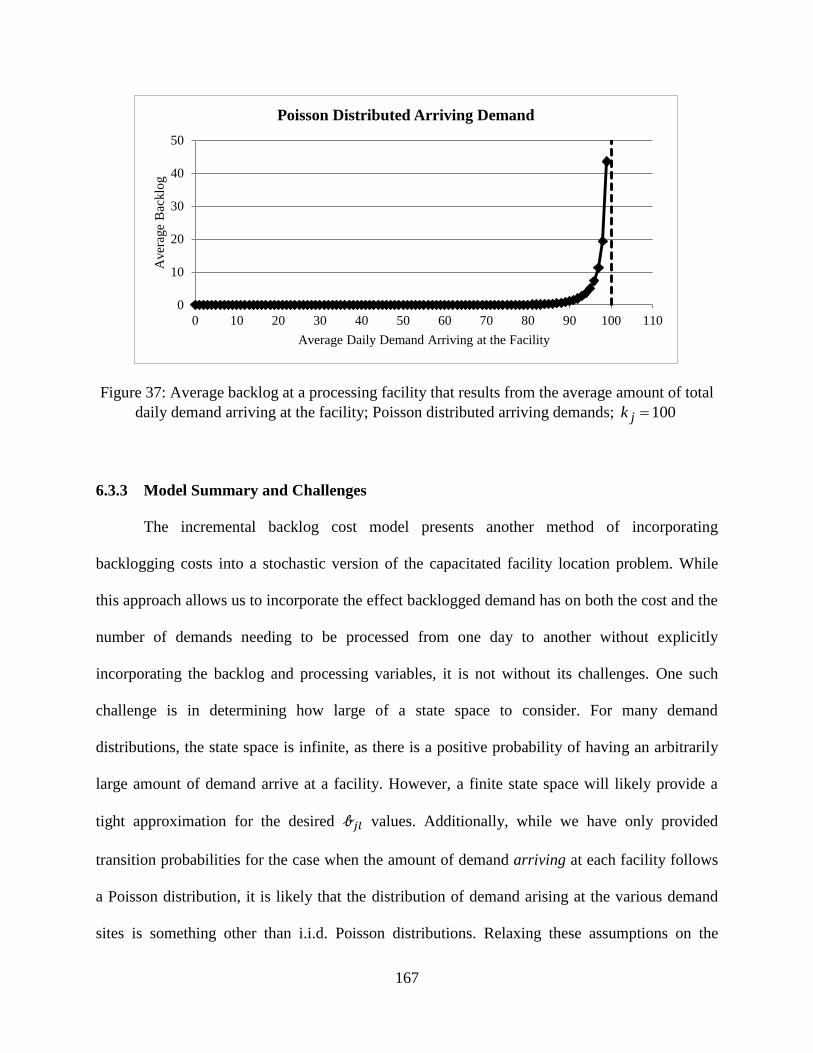
167
Figure 37: Average backlog at a processing facility that results from the average amount of total
daily demand arriving at the facility; Poisson distributed arriving demands; 100jk
6.3.3 Model Summary and Challenges
The incremental backlog cost model presents another method of incorporating
backlogging costs into a stochastic version of the capacitated facility location problem. While
this approach allows us to incorporate the effect backlogged demand has on both the cost and the
number of demands needing to be processed from one day to another without explicitly
incorporating the backlog and processing variables, it is not without its challenges. One such
challenge is in determining how large of a state space to consider. For many demand
distributions, the state space is infinite, as there is a positive probability of having an arbitrarily
large amount of demand arrive at a facility. However, a finite state space will likely provide a
tight approximation for the desired 𝒷𝑗𝑙 values. Additionally, while we have only provided
transition probabilities for the case when the amount of demand arriving at each facility follows
a Poisson distribution, it is likely that the distribution of demand arising at the various demand
sites is something other than i.i.d. Poisson distributions. Relaxing these assumptions on the
0
10
20
30
40
50
0 10 20 30 40 50 60 70 80 90 100 110
Aver
age
Bac
klo
g
Average Daily Demand Arriving at the Facility
Poisson Distributed Arriving Demand

168
demand distributions pose additional analytical challenges as the decision regarding the
allocation of demand sites (which may have spatially or temporally correlated demand as well as
each having a different distribution of demand) directly impacts the distribution of the demand
arriving at each processing facility.
6.4 Outbound Shipment Model
Thus far we have presented and discussed models that mitigate hard capacity constraints
in the context of a system with physical demand (e.g., blood samples) that arrives at a processing
facility (e.g., blood testing facility) and has intangible results (e.g., a report) that are reported to
the customer. Incoming demands that exceed the daily processing capacity are physically held as
backlog (at some cost) and are processed at a later date. However, with a slight change of
notation we can modify the formulation to represent a system in which warehouses receive
intangible demand orders and must ship physical goods to the demand sites. (Online retailers,
including Amazon.com, are often examples of such a system.) The warehouse may have a policy
that orders must be shipped within one day of the order being placed (i.e., the order needs to be
en route to the demand site within one day; it does not have to arrive at the demand site within
one day). If an item cannot be shipped within the specified timeframe, a penalty cost is incurred
to account for expedited shipping or loss of goodwill. We refer to such an item as a “late item.”
The goal is to determine where to build warehouses and how to assign warehouses to demand
sites so that the total location, transportation, and penalty cost is minimized, while ensuring that a
specified service level is achieved.

169
Stochastic IMCLP Outbound Shipment Formulation
Letting 𝐽 represent the set of candidate warehouse locations and 𝐼 the set of demand sites,
we can modify the original stochastic IMCLP notation to fit the outbound shipment context.
While we present the model with the joint chance constraints, we note that substituting the
hybrid or individual chance constraints for the joint chance constraint results in the
corresponding outbound shipment formulation.
Modified Parameters
𝑘𝑗 Capacity of warehouse 𝑗 ∈ 𝐽 in items shipped per day
𝑏 ≥ 0 Penalty cost (in dollars) of shipping one item one day late
𝜃 At any given time, the maximum desired number of late items at an individual warehouse
𝜏 Maximum acceptable probability of having more than 𝜃 late items at any facility on any
day
𝑣𝑗 Initial number of late items at warehouse 𝑗 ∈ 𝐽 if warehouse 𝑗 is located
Decision Variables
𝑋𝑗 = 1
0
If we locate at warehouse 𝑗 ∈ 𝐽
Otherwise
𝑌𝑖𝑗 = 1
0
If we assign warehouse 𝑗 ∈ 𝐽 to fulfill demand from 𝑖 ∈ 𝐼
Otherwise
𝑉𝑗𝑑𝜔 Number of late items at warehouse 𝑗 ∈ 𝐽 at the beginning of day 𝑑 ∈ 𝐷 ∪ (|𝐷| + 1) in
scenario 𝜔 ∈ Ω
𝑊𝑗𝑑𝜔 Number of items that are shipped from warehouse 𝑗 ∈ 𝐽 on day 𝑑 ∈ 𝐷 in scenario 𝜔 ∈ Ω

170
The modified model becomes:
[M-JCC]:
𝑀𝑖𝑛 𝑿,𝒀,𝑽,𝑾 |𝐷|∑ 𝑓𝑗𝑋𝑗𝑗∈𝐽 + 𝑎∑ ∑ ∑ 𝔼𝜉[ℎ𝑖𝑑]𝑡𝑖𝑗𝑌𝑖𝑗𝑗∈𝐽|𝐷|𝑑=1𝑖∈𝐼 + 𝑏 𝔼𝜉[∑ ∑ 𝑗𝑑𝑗∈𝐽
|𝐷|+1𝑑=2 ] (6.8)
Subject to
∑ 𝑌𝑖𝑗𝑗∈𝐽 = 1 ∀𝑖 ∈ 𝐼 (2.2)
𝑌𝑖𝑗 − 𝑋𝑗 ≤ 0 ∀𝑖 ∈ 𝐼; 𝑗 ∈ 𝐽 (2.3)
ℙ(𝑗𝑑 ≤ 𝜃; ∀𝑗 ∈ 𝐽; 𝑑 ∈ 𝐷 ∪ (|𝐷| + 1)) ≥ 1 − 𝜏 (6.9)
𝑉𝑗,𝑑+1𝜔 − 𝑉𝑗𝑑
𝜔 +𝑊𝑗𝑑𝜔 = ∑ ℎ𝑖𝑑
𝜔𝑌𝑖𝑗𝑖∈𝐼 ∀𝑗 ∈ 𝐽; 𝑑 ∈ 𝐷;𝜔 ∈ Ω (6.10)
𝑊𝑗𝑑𝜔 ≤ 𝑘𝑗𝑋𝑗 ∀𝑗 ∈ 𝐽; 𝑑 ∈ 𝐷;𝜔 ∈ Ω (6.11)
𝑉𝑗,1𝜔 = 𝑣𝑗𝑋𝑗 ∀𝑗 ∈ 𝐽; 𝜔 ∈ Ω (6.12)
𝑉𝑗𝑑𝜔 ≥ 0 ∀𝑗 ∈ 𝐽; 𝑑 ∈ 𝐷 ∪ (|𝐷| + 1);𝜔 ∈ Ω (6.13)
𝑊𝑗𝑑𝜔 ≥ 0 ∀𝑗 ∈ 𝐽; 𝑑 ∈ 𝐷;𝜔 ∈ Ω (6.14)
𝑋𝑗 ∈ 0,1 ∀𝑗 ∈ 𝐽 (2.4)
𝑌𝑖𝑗 ∈ 0,1 ∀𝑖 ∈ 𝐼; 𝑗 ∈ 𝐽 (3.6)
The major difference between the JCC formulation and the modified M-JCC is that the
new formulation does not have incoming demand that is being shipped from the demand sites to
the warehouses. Instead, the warehouses ship the demand to the demand sites. Thus, we do not
need to include a warm-up period in formulation M-JCC. (Note that the time horizon is now |𝐷|
rather than |𝐷| − 𝑡∗). Additionally, constraints (6.10) use the demand that is generated on day 𝑑
to calculate the number of late items on day 𝑑 + 1, rather than using demand that was generated
𝑑 − 𝑡𝑖𝑗 days ago. We use constraints (6.12) to initialize the number of late items at the beginning
of the horizon. Additionally, the joint chance constraint represented by (6.9) now states that there

171
cannot be more than 𝜃 late items present at any warehouse on any day in more than 𝜏 ∗ 100% of
the scenarios. If a scenario contains one year’s worth of data and the model contains ten
scenarios, this is equivalent to saying that we must always have less than 𝜃 late items in at least
⌊(1 − 𝜏) ∗ 10⌋ of the years.
Cyclic Allocation Outbound Shipment Formulation
A similar outbound shipment perspective can be formulated for the IMCLP with cyclic
allocations. In addition to the modified notation already discussed, we introduce the redefined
sets, parameters, and decision variables:
Modified Sets and Parameters
𝐷𝑝 ≔ 𝑑 ∈ 𝐷: 𝑑 𝑚𝑜𝑑 |𝑃| = 𝑝 Set of days in 𝐷 corresponding to cycle day 𝑝 ∈ 𝑃
𝑘𝑗𝑝 Capacity of warehouse 𝑗 ∈ 𝐽 on cycle day 𝑝 ∈ 𝑃 in terms of items shipped per day
Decision Variables
𝑌𝑖𝑗𝑝 =
1
0
If we assign warehouse 𝑗 ∈ 𝐽 to fulfill demand from 𝑖 ∈ 𝐼 on cycle day 𝑝 ∈ 𝑃
Otherwise
The outbound IMCLP cyclic allocation model can then be presented as:
𝑀𝑖𝑛 𝑿,𝒀,𝑽,𝑾 |𝐷|∑ 𝑓𝑗𝑋𝑗𝑗∈𝐽 + 𝑎∑ ∑ ∑ ∑ ℎ𝑖𝑑𝑡𝑖𝑗𝑌𝑖𝑗𝑝
𝑖∈𝐼𝑗∈𝐽𝑑∈𝐷𝑝𝑝∈𝑃 + 𝑏∑ ∑ 𝑉𝑗𝑑𝑗∈𝐽|𝐷|+1𝑑=2 (6.15)
𝑆𝑢𝑏𝑗𝑒𝑐𝑡 𝑡𝑜
∑ 𝑌𝑖𝑗𝑝
𝑗∈𝐽 = 1 ∀𝑖 ∈ 𝐼; 𝑝 ∈ 𝑃 (4.2)
𝑌𝑖𝑗𝑝 ≤ 𝑋𝑗 ∀𝑖 ∈ 𝐼; 𝑗 ∈ 𝐽; 𝑝 ∈ 𝑃 (4.3)
𝑉𝑗,𝑑+1 = 𝑉𝑗𝑑 + ∑ ℎ𝑖,𝑑𝑌𝑖𝑗 𝑑 𝑚𝑜𝑑 |𝑃|
𝑖∈𝐼 −𝑊𝑗𝑑 ∀𝑗 ∈ 𝐽; 𝑑 ∈ 𝐷 (6.16)
𝑊𝑗𝑑 ≤ 𝑘𝑗𝑝𝑋𝑗 ∀𝑗 ∈ 𝐽; 𝑝 ∈ 𝑃; 𝑑 ∈ 𝐷𝑝 (4.5)
𝑉𝑗,1 = 𝑣𝑗𝑋𝑗 ∀𝑗 ∈ 𝐽 (6.17)

172
𝑋𝑗 ∈ 0,1 ∀𝑗 ∈ 𝐽 (2.4)
𝑌𝑖𝑗𝑝 ∈ 0,1 ∀𝑖 ∈ 𝐼; 𝑗 ∈ 𝐽; 𝑝 ∈ 𝑃 (4.6)
𝑉𝑗𝑑 ≥ 0 ∀𝑗 ∈ 𝐽; 𝑑 ∈ 𝐷 ∪ (|𝐷| + 1) (6.18)
𝑊𝑗𝑑 ≥ 0 ∀𝑗 ∈ 𝐽; 𝑑 ∈ 𝐷 (6.19)
6.5 Additional Methods of Incorporating Capacity Flexibility
This dissertation has focused on incorporating short-term capacity flexibility into facility
location models by allowing a processing facility to accept demands in excess of its processing
capacity and store the excess demand in backlog until it can be processed. While this is one way
of incorporating capacity flexibility, there are numerous other avenues that are used in practice.
For example, a processing facility may utilize employee overtime, hire temporary workers,
outsource excess demands, or add additional physical capacity (e.g., an additional processing
machine or assembly line) to capture endogenous capacity flexibility. Additionally, exogenous
capacity flexibility can be captured through stochastic programming. In this section we formulate
extensions to the IMCLP that incorporate both endogenous and exogenous methods of capturing
capacity flexibility.
6.5.1 Endogenous Capacity Flexibility
Rather than requiring all demand in excess of the processing capacity to be held in
backlog, we can formulate an extension to the IMCLP which allows extra daily capacity to be
purchased on a day-to-day basis. In this model, processing facility 𝑗 ∈ 𝐽 starts each day with the
capacity to process 𝑘𝑗 items. However, if the arriving demand exceeds the processing capacity,
the facility manager at 𝑗 ∈ 𝐽 has the option of purchasing extra capacity for that day at a unit cost

173
of 𝑗 rather than incurring a facility specific backlog penalty cost 𝑏𝑗. In this discussion, we
assume that the extra capacity can be purchased after the daily amount of arriving demand is
realized. However, a stochastic extension can also be formulated to address the situation in
which a facility manager must decide one day in advance (before knowing the exact amount of
incoming demand) how much extra capacity to purchase. We leave this extension as an area of
future work.
We let 𝑗𝑑 be a non-negative decision variable that represents the extra capacity to
purchase at facility 𝑗 ∈ 𝐽 on day 𝑑 ∈ 𝑡∗ + 1,… , |𝐷| and 𝑘𝑗𝑚𝑎𝑥 ≥ 0 be a parameter representing
the maximum amount of additional capacity facility 𝑗 ∈ 𝐽 can purchase each day (𝑘𝑗𝑚𝑎𝑥 may be
unbounded from above). We formulate the model as follows:
𝑀𝑖𝑛𝑿,𝒀,𝑽,𝑾,(|𝐷| − 𝑡∗)∑ 𝑓𝑗𝑋𝑗𝑗∈𝐽 + 𝑎∑ ∑ ∑ ℎ𝑖𝑑𝑡𝑖𝑗𝑌𝑖𝑗𝑖∈𝐼𝑗∈𝐽
|𝐷|𝑑=𝑡∗+1 + ∑ ∑ 𝑏𝑗𝑉𝑗𝑑𝑗∈𝐽
|𝐷|+1𝑑=𝑡∗+2
+∑ ∑ 𝑗𝑗𝑑𝑗∈𝐽|𝐷|𝑑=𝑡∗+1 (6.20)
𝑆𝑢𝑏𝑗𝑒𝑐𝑡 𝑡𝑜
∑ 𝑌𝑖𝑗𝑗∈𝐽 = 1 ∀𝑖 ∈ 𝐼 (2.2)
𝑌𝑖𝑗 ≤ 𝑋𝑗 ∀𝑖 ∈ 𝐼; 𝑗 ∈ 𝐽 (2.3)
𝑉𝑗,𝑑+1 − 𝑉𝑗𝑑 − ∑ ℎ𝑖,𝑑−𝑡𝑖𝑗𝑌𝑖𝑗𝑖∈𝐼 +𝑊𝑗𝑑 = 0 ∀𝑗 ∈ 𝐽; 𝑑 ∈ 𝑡∗ + 1,… , |𝐷| (3.3)
𝑗𝑑 ≤ 𝑘𝑗𝑚𝑎𝑥𝑋𝑗 ∀𝑗 ∈ 𝐽; 𝑑 ∈ 𝑡∗ + 1,… , |𝐷| (6.21)
𝑊𝑗𝑑 ≤ 𝑘𝑗𝑋𝑗 + 𝑗𝑑 ∀𝑗 ∈ 𝐽; 𝑑 ∈ 𝑡∗ + 1,… , |𝐷| (6.22)
𝑉𝑗,𝑡∗+1 = 𝑣𝑗𝑋𝑗 ∀𝑗 ∈ 𝐽 (3.5)
𝑋𝑗 ∈ 0,1 ∀𝑗 ∈ 𝐽 (2.4)
𝑌𝑖𝑗 ∈ 0,1 ∀𝑖 ∈ 𝐼; 𝑗 ∈ 𝐽 (3.6)
𝑉𝑗𝑑 ≥ 0 ∀𝑗 ∈ 𝐽; 𝑑 ∈ 𝑡∗ + 1,… , |𝐷| + 1 (3.7)

174
𝑊𝑗𝑑 ≥ 0 ∀𝑗 ∈ 𝐽; 𝑑 ∈ 𝑡∗ + 1,… , |𝐷| (3.8)
𝑗𝑑 ≥ 0 ∀𝑗 ∈ 𝐽; 𝑑 ∈ 𝑡∗ + 1,… , |𝐷| (6.23)
Alternatively, extra daily capacity may only be available to purchase in increments of size 𝑗.
Thus, some of the purchased extra capacity may be unused at the end of the day. To amend the
above model to account for incremental daily capacity, let 𝑗𝑑 be a nonnegative integer decision
variable indicating the number of increments purchased, replace 𝑗𝑑 with 𝑗𝑗𝑑 in (6.20) -
(6.22), and replace constraint (6.23) with
𝑗𝑑 ≥ 0, 𝑖𝑛𝑡𝑒𝑔𝑒𝑟 ∀𝑗 ∈ 𝐽; 𝑑 ∈ 𝑡∗ + 1,… , |𝐷| (6.24)
While the aforementioned models allow capacity to be added on a day-by-day basis, the
facility manager may not have the ability to change the capacity each day of the planning
horizon. Instead, the manager may prefer a cyclic method of adding capacity in which facility
𝑗 ∈ 𝐽 has a base capacity to process 𝑘𝑗 items each day and the option to increase capacity by 𝑗𝑝
(a decision variable) on cycle day 𝑝 ∈ 𝑃 at a cost of 𝑗 per unit of capacity increase. The cyclic
method of adding capacity can be incorporated into the cyclic allocation model by adding the
term ∑ ∑ 𝑗𝑗𝑝
𝑗∈𝐽 |𝐷𝑝|𝑝∈𝑃 to objective function (4.1), adding 𝑗𝑝 to the right hand side of
constraint (4.5), and adding constraints
𝑗𝑝 ≤ 𝑘𝑗
𝑚𝑎𝑥𝑋𝑗 ∀𝑗 ∈ 𝐽; 𝑝 ∈ 𝑃 (6.25)
and
𝑗𝑝≥ 0, 𝑖𝑛𝑡𝑒𝑔𝑒𝑟 ∀𝑗 ∈ 𝐽; 𝑝 ∈ 𝑃. (6.26)

175
6.5.2 Exogenous Capacity Fluctuations
While facility managers may have many methods of affecting the amount of capacity
available each day, there also exist exogenous capacity fluctuations that managers have very
little (if any) control over. Examples of such exognous fluctuations include capacity degregations
due to machine breakdowns and quality control issues. Workers who assemble products or pick
customer orders in a warehouse also add an element of uncertainty because each employee
completes tasks at a different rate.
In this section we will present two extensions of the IMCLP that incorporate exogenous
capacity fluctuations. The first is a stochastic version of the IMCLP in which the capacity is an
uncertain model input. While this formulation will not incorporate uncertain demand as we do in
Chapter 5, models that incorporate both uncertain demand and capacity can be developed by
merging the two stochstic formulations. The second extension depicts employee training by
modeling capacity that increases naturally over a period of time during the training period and
eventually reaches some asymptotic behavior when the employees are fully trained.
Stochastic Daily Capacity
Let Ω represent the finite set of all possible capacity scenarios, and represent the
probability of a particular scenario ∈ Ω. The parameter 𝑗𝑑 corresponds to the random daily
capacity available at processing facility 𝑗 ∈ 𝐽 on day 𝑑 ∈ 𝑡∗ + 1,… , |𝐷|. While 𝑗𝑑 is a random
parameter, 𝑗𝑑 represents a realization of the random capacity 𝑗𝑑 available at facility 𝑗 ∈ 𝐽 on
day 𝑑 ∈ 𝑡∗ + 1,… , |𝐷| in scenario ∈ Ω. We also let () ∈ ℕ0|𝐽|×|𝐷|
be a vector containing
the capacity realizations 𝑗𝑑 , ∀𝑗 ∈ 𝐽, 𝑑 ∈ 𝑡∗ + 1,… , |𝐷| corresponding to scenario ∈ Ω.
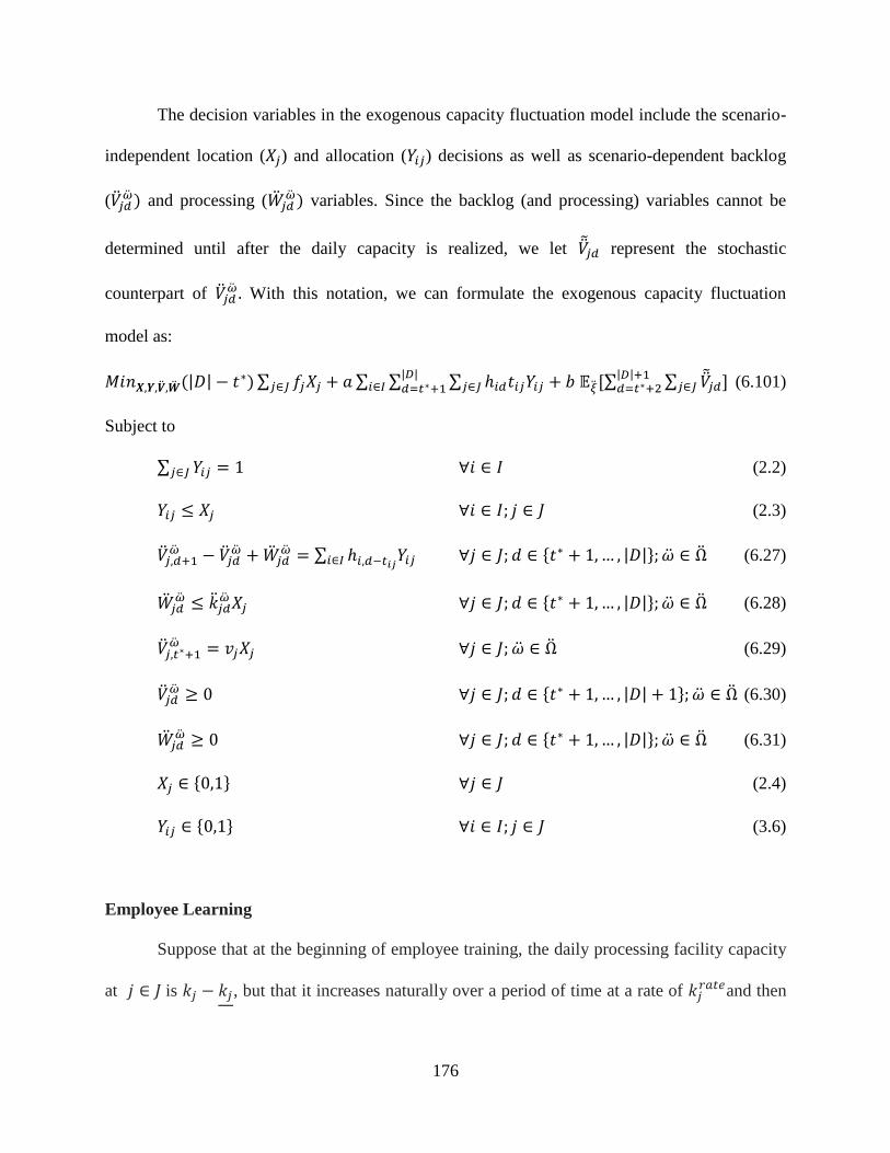
176
The decision variables in the exogenous capacity fluctuation model include the scenario-
independent location (𝑋𝑗) and allocation (𝑌𝑖𝑗) decisions as well as scenario-dependent backlog
(𝑗𝑑) and processing (𝑗𝑑
) variables. Since the backlog (and processing) variables cannot be
determined until after the daily capacity is realized, we let 𝑗𝑑 represent the stochastic
counterpart of 𝑗𝑑 . With this notation, we can formulate the exogenous capacity fluctuation
model as:
𝑀𝑖𝑛𝑿,𝒀,,(|𝐷| − 𝑡∗)∑ 𝑓𝑗𝑋𝑗𝑗∈𝐽 + 𝑎∑ ∑ ∑ ℎ𝑖𝑑𝑡𝑖𝑗𝑌𝑖𝑗𝑗∈𝐽
|𝐷|𝑑=𝑡∗+1𝑖∈𝐼 + 𝑏 𝔼[∑ ∑ 𝑗𝑑𝑗∈𝐽
|𝐷|+1𝑑=𝑡∗+2 ] (6.101)
Subject to
∑ 𝑌𝑖𝑗𝑗∈𝐽 = 1 ∀𝑖 ∈ 𝐼 (2.2)
𝑌𝑖𝑗 ≤ 𝑋𝑗 ∀𝑖 ∈ 𝐼; 𝑗 ∈ 𝐽 (2.3)
𝑗,𝑑+1 − 𝑗𝑑
+ 𝑗𝑑 = ∑ ℎ𝑖,𝑑−𝑡𝑖𝑗
𝑌𝑖𝑗𝑖∈𝐼 ∀𝑗 ∈ 𝐽; 𝑑 ∈ 𝑡∗ + 1,… , |𝐷|; ∈ Ω (6.27)
𝑗𝑑 ≤ 𝑗𝑑
𝑋𝑗 ∀𝑗 ∈ 𝐽; 𝑑 ∈ 𝑡∗ + 1,… , |𝐷|; ∈ Ω (6.28)
𝑗,𝑡∗+1 = 𝑣𝑗𝑋𝑗 ∀𝑗 ∈ 𝐽; ∈ Ω (6.29)
𝑗𝑑 ≥ 0 ∀𝑗 ∈ 𝐽; 𝑑 ∈ 𝑡∗ + 1,… , |𝐷| + 1; ∈ Ω (6.30)
𝑗𝑑 ≥ 0 ∀𝑗 ∈ 𝐽; 𝑑 ∈ 𝑡∗ + 1,… , |𝐷|; ∈ Ω (6.31)
𝑋𝑗 ∈ 0,1 ∀𝑗 ∈ 𝐽 (2.4)
𝑌𝑖𝑗 ∈ 0,1 ∀𝑖 ∈ 𝐼; 𝑗 ∈ 𝐽 (3.6)
Employee Learning
Suppose that at the beginning of employee training, the daily processing facility capacity
at 𝑗 ∈ 𝐽 is 𝑘𝑗 − 𝑘𝑗 , but that it increases naturally over a period of time at a rate of 𝑘𝑗𝑟𝑎𝑡𝑒and then

177
remains at a constant level, 𝑘𝑗, when employees have been fully trained on the work processes.
We can model such a situation as an exponential increase in capacity and can easily implement
this into the IMCLP by changing constraint (3.4) from
𝑊𝑗𝑑 ≤ 𝑘𝑗𝑋𝑗 ∀𝑗 ∈ 𝐽; 𝑑 ∈ 𝑡∗ + 1,… , |𝐷| (3.4)
to
𝑊𝑗𝑑 ≤ (𝑘𝑗 − 𝑘𝑗𝑒−𝑘𝑗
𝑟𝑎𝑡𝑒(𝑑−(𝑡∗−1)))𝑋𝑗 ∀𝑗 ∈ 𝐽; 𝑑 ∈ 𝑡∗ + 1,… , |𝐷|. (6.32)
6.6 Conclusions and Contributions
This dissertation argued that the hard capacity constraints that are often employed in
location modeling are unrealistic since facility managers have numerous operational tools that
allow a facility to accept items in excess of the stated processing capacity level. As such, we
developed a new approach to modeling capacitated facility location models that takes into
account the likelihood that the total amount of demand arriving at a processing facility may
exceed the daily processing capacity on any day of the planning horizon. When such
exceedances occur, our models permit backlogging excess demands and processing them at a
later date. To ensure adequate service metrics are met, we assess a daily penalty cost for each
unit of backlogged demand and, in models that consider stochastic demands, we also
incorporated chance constraints to impose limits on the quantity of backlogged demand.
We reported the difference in facility locations, demand allocations, and total cost
between the CFLP and our IMCLP approach. In particular, we have shown that the CFLP and
IMCLP often do not locate the same facilities (and in some instances they locate a different
number of facilities), and therefore also do not allocate demands to the same processing
facilities. Since the CFLP does not incorporate the cost of backlog, the CFLP underestimates the

178
total cost. The cost benefit of using the IMCLP instead of the CFLP is particularly notable for
application contexts in which it is highly desirable to process all of the demands on the day they
arrive at a processing facility. Such an underestimate could have significant implications on
budget predictions.
A key benefit of the IMCLP model is that it incorporates the penalty cost associated with
the reality that on some days the total amount of demand arriving at a processing facility may
exceed the daily processing capacity. The IMCLP formulation inherently assumes that demands
do not expire; demands can be postponed indefinitely as long as the penalty cost is paid. We
realize that in many situations this is not realistic and presented additional constraints that could
be added to ensure demands are processed within a specified amount of time.
Our model formulations can use a dataset as a direct input into the model rather than
specifying deterministic demands at an aggregate level by using parameter estimation
techniques. This enabled us to develop a day-of-the-week allocation policy that considers day-to-
day variations in the daily processing capacity levels of a set of candidate processing facilities
and/or systematic day-to-day demand variations. For example, our model is able to adjust the
allocation policy to account for some facilities being closed on weekends or for days of the week
that generate more demand than other days of the week. Through computational studies, we
showed that incorporating this cyclic allocation approach into the model resulted in a significant
cost savings as compared to models that do not incorporate this approach, such as the IMCLP.
Furthermore, we noted that the model can readily be restructured to deal with other cycles, such
as annual cycles with demand assignments that either change seasonally or monthly in response
to time-varying demand patterns.

179
We also presented multiple constraints that can be added to the model formulation to
achieve various operational goals. These include (1) restricting the number of processing
facilities to which a demand site can be assigned, (2) introducing a weekday/weekend allocation
policy, and (3) restricting the maximum allowed travel time. Our results suggest that a significant
cost benefit can be achieved by implementing the cyclic allocation model as compared to
capacitated facility location models that require a static allocation policy. Much of this benefit
can be achieved even when additional constraints of the form outlined above are imposed.
While the IMCLP and IMCLP with cyclic allocations consider deterministic demands,
our third modeling framework incorporated demand stochasticity into the IMCLP using a
scenario based stochastic optimization approach in which a scenario corresponds to a realization
of the daily demand for every day within the time horizon. In addition to assessing a penalty cost
associated with each day an item spends in backlog (as is done in the IMCLP), we considered
three different types of chance constraints to restrict the number of demands that are backlogged
to a predetermined threshold. We first incorporated joint chance constraints that ensure the
probability of any processing facility having a backlog level above the threshold on any day of
the planning horizon is sufficiently small. We also modelled individual chance constraints on the
amount of backlog at each facility each day, as well as a hybrid approach that accounts for the
number of processing facilities that exceed the stated maximum backlog level on any day of the
planning horizon. We then presented mixed-integer programming reformulations of the chance
constraints that incorporate a finite number of scenarios from a given known demand
distribution.
Through computational experiments, we showed that the stochastic, chance constrained
version of the IMCLP can produce different location and allocation solutions than the IMCLP,

180
and that even small differences in their allocations can drastically impact the amount of items
held in backlog. Furthermore, if the decision maker has a limit on the desired maximum amount
if items backlogged at any given time, it is important that the decision maker utilize the
stochastic model; imposing the limit on a single demand scenario (i.e., using the IMCLP) often
resulted in infeasible solutions to the joint chance constrained stochastic IMCLP due to the
demand uncertainty.
The resulting models were solved using two different decomposition schemes and their
performance is compared to that of a generic solver. The first approach decomposed the problem
into two stages: the long-term (i.e., location and allocation) decisions were determined in the first
stage while the daily (i.e., processing and backlog) decisions were determined in the second
stage. Benders decomposition was used to solve the resulting formulation. The second
decomposition scheme capitalized on the problem structure by utilizing a three-stage structure.
In particular, given a feasible first-stage location and allocation solution, we readily determined
the optimal second-stage processing and backlog decisions as well as the third-stage auxiliary
variables that verify whether the joint chance constraint is satisfied by inspection. If the joint
chance constraint was violated, a corresponding cut was added to the first-stage problem.
Computational results for the IMCLP, IMCLP with cyclic allocations, and the chance
constrained IMCLP were presented for large-scale data sets generated from 2010 U.S. census
population data by county. Using diverse data instances, we demonstrated the benefits gained
from using a data-driven model with short term capacity flexibility. In each of these modelling
contexts, we showed that the location and allocation decisions obtained from our models can
result in significantly reduced costs and improved service metrics when compared to traditional
models that do not account for the likelihood that demands may exceed capacity on some days.

181
Finally, we presented a number of avenues for future research including a queueing
approach, incremental backlog cost model, and an outbound shipment model. Furthermore,
although the focus of this dissertation was the effect of incorporating the option to backlog
excess demands, managers have additional operational tools that relax the traditional inflexible
capacity constraints, including overtime, adding additional production shifts, and outsourcing.
Degradations in capacity are also a reality. That is, the actual capacity on any day may be less
than the nominal capacity due to machine breakdowns, labor slowdowns, or power outages. As
such, we briefly discussed formulations for incorporating additional types of exogenous and
endogenous capacity flexibility into a data-driven capacitated facility location model.

182
APPENDICES

183
APPENDIX A: The Data-Driven CFLP
We formulate the data-driven CFLP as follows:
𝑀𝑖𝑛 𝑿,𝒀 (|𝐷| − 𝑡∗)∑ 𝑓𝑗𝑋𝑗𝑗∈𝐽 + 𝑎∑ ∑ ∑ ℎ𝑖𝑑𝑡𝑖𝑗𝑌𝑖𝑗𝑖∈𝐼𝑗∈𝐽
|𝐷|𝑑=𝑡∗+1 (A.1)
𝑆𝑢𝑏𝑗𝑒𝑐𝑡 𝑡𝑜
∑ 𝑌𝑖𝑗𝑗∈𝐽 = 1 ∀𝑖 ∈ 𝐼 (2.2)
𝑌𝑖𝑗 ≤ 𝑋𝑗 ∀𝑖 ∈ 𝐼; 𝑗 ∈ 𝐽 (2.3)
∑ ℎ𝑖,𝑑−𝑡𝑖𝑗𝑌𝑖𝑗𝑖∈𝐼 ≤ 𝑘𝑗𝑋𝑗 ∀𝑗 ∈ 𝐽; 𝑑 ∈ 𝑡∗ + 1,… , |𝐷| (A.2)
𝑋𝑗 ∈ 0,1 ∀𝑗 ∈ 𝐽 (2.4)
𝑌𝑖𝑗 ∈ 0,1 ∀𝑖 ∈ 𝐼; 𝑗 ∈ 𝐽 (3.6)
The objective function (A.1) minimizes the sum of the fixed facility and transportation costs over
a time horizon of (|𝐷| − 𝑡∗) days. We note that the second term of the objective function
includes the daily demands, ℎ𝑖𝑑, rather than the aggregated average demand, ℎ𝑖, used in the
CFLP objective function (3.1). Constraints (2.2) and (2.3), respectively, ensure that each demand
site 𝑖 ∈ 𝐼 is assigned to exactly one facility and that demands can only be assigned to located
facilities. Constraints (A.2) are the data-driven capacity constraints that limit the amount of
demand that arrives at a processing facility to be no more than the daily processing capacity of
the facility. Thus, all demands are able to be processed on the day they arrive. Constraints (A.2)
differ from the CFLP capacity constraints (2.6) in that constraints (A.2) are enforced on the

184
individual daily demands while constraints (2.6) are enforced on the average demands.
Constraints (2.4) and (3.6) are standard binary and non-negativity constraints, as in the CFLP.

185
APPENDIX B: Effect of Population Weight
As discussed in Section 3.4, the daily facility location costs are calculated by specifying a
daily base cost plus an additional cost calculated form the associated demand (population)
generated at that location. Specifically, we use the formula
𝑧 + 𝑤𝜌𝑗
to generate the daily facility location cost for each facility 𝑗 ∈ 𝐽, where 𝑧 denotes the daily base
fixed cost, 𝜌𝑗 represents the population of the candidate processing facility 𝑗, and 𝑤 is the
population weight.
Table 34 describes the effect of the population weight on the daily facility location cost
parameters, as well as the optimal IMCLP solution for the 50 demand, 50 candidate node
instance, a daily base fixed cost of 𝑧 = $10,000, Poisson distributed daily demands with a mean
equal to 1/10,000 of the county population, and unit transportation and backlogging costs of
𝑎 = 1 and 𝑏 = 3, respectively. The first column indicates the weight attributed to the population.
The second and third columns display the daily facility location cost of the least costly (Node 50:
Du Page, IL) and most costly (Node 1: Los Angeles, CA) candidate processing facilities. Notice
that as the population weight increases, the disparity between the minimum and maximum costs
increases, as does the average daily facility location cost of the candidate facilities (column 4).
The optimal solution for all five values of 𝑤 locates five processing facilities. The fifth column
enumerates the ranks of the five facilities that are located (recall that that lower ranks have a
higher facility location cost), the sixth column reports the average of the five ranks, and the last
column displays the average daily facility location cost of the facilities that are located in the

186
optimal solution. As expected, when the population weight, 𝑤, increases, it becomes essential to
locate at less expensive candidate processing facilities (i.e., higher ranked facilities). Maps of the
optimal facility locations are presented in Figure 38.
Table 34: Effect of population weight on location cost and optimal solution; Poisson distributed
demand; a=1, b=3 Daily Facility Location Cost
Parameters
Optimal Solution
𝑤 Min
(Node 50)
Max
(Node 1) Avg.
Ranks Located
Avg.
Rank
Located
Avg. Daily
Cost of
Located
$0 $10,000 $10,000 $10,000 1, 2, 3, 7, 13 5.2 $10,000
$0.0001 $10,092 $10,982 $10,183 2, 3, 6, 7, 13 6.2 $10,335
$0.001 $10,917 $19,819 $11,833 12, 39, 43, 45, 50 37.8 $11,171
$0.01 $19,169 $108,186 $28,331 39, 41, 43, 45, 50 43.6 $19,602
$0.1 $101,692 $991,861 $193,311 41, 45, 47, 49, 50 46.4 $103,345

187
Figure 38: The optimal facility locations listed in Table 34
1
13
3
7
2
6
13
3
7
2
45
12 39
50
43
50
43
39
45
41
45
41 47
50 49
𝒘 = $𝟎 𝒘 = $𝟎. 𝟎𝟎𝟎𝟏
𝒘 = $𝟎. 𝟎𝟎𝟏 𝒘 = $𝟎. 𝟎𝟏
𝒘 = $𝟎. 𝟏

188
APPENDIX C: Proof of the Validity of Feasibility Cuts (5.89)
Individual Chance Constraints
To show the validity of cut (5.89) we begin by recalling 𝐼𝜓≔ 𝑖 ∈ 𝐼: 𝑌𝑖𝑗
𝜓= 1 represents
demand sites allocated to processing facility 𝑗 ∈ 𝐽 in infeasible solution 𝜓 ∈ Ψ𝑗. Let ℱ ≔
(𝑿, 𝒀): ∃𝑽,𝑾, 𝒁: (2.2) - (2.4), (3.6), (5.15) - (5.19), (5.22), and (5.80) - (5.82) are satisfied.
For any feasible (𝑿, 𝒀) solution to MIP-ICC, (𝑿, 𝒀) ∈ ℱ. Suppose another solution, (𝑿𝜓, 𝒀𝜓)
satisfies constraints (2.2) - (2.4), (3.6), and (5.22) but (𝑿𝜓, 𝒀𝜓) ∉ ℱ. It follows that (𝑿, 𝒀) ≠
(𝑿𝜓, 𝒀𝜓).
This further implies that the allocation decisions corresponding to the two solutions are
different, i.e., 𝒀 ≠ 𝒀𝜓. To see this, note that if 𝑿 = 𝑿𝝍, then it must be that 𝒀 ≠ 𝒀𝜓 in order for
(𝑿, 𝒀) ≠ (𝑿𝜓, 𝒀𝜓). If instead 𝑿 ≠ 𝑿𝝍, then ∃𝑗 ∈ 𝐽 such that 𝑋 ≠ 𝑋𝜓
. Thus, either 𝑋 = 1 and
𝑋𝜓= 0, or 𝑋 = 0 and 𝑋
𝜓= 1. Suppose 𝑋 = 1 and 𝑋
𝜓= 0. Then, for every 𝑖 ∈ 𝐼 such that
𝑌𝑖 = 1 we must have 𝑌𝑖𝜓= 0 since facility 𝑗 is not located in solution (𝑿𝜓, 𝒀𝜓). Thus, 𝒀 ≠ 𝒀𝜓.
An analogous reasoning holds for the case of 𝑋 = 0 and 𝑋𝜓= 1.
Furthermore, the reason (𝑿𝜓, 𝒀𝜓) ∉ ℱ must be because it violates the collective group of
constraints (5.80) - (5.82). Since (𝑿, 𝒀) is a feasible solution to MIP-ICC, there must exist 𝑖′ ∈ 𝐼
such that 𝑌𝑖′
𝜓= 1 and 𝑌𝑖′ = 0 for some 𝑗 ∈ 𝐽 and ∈ 𝑡∗ + 1,… , |𝐷| + 1 with
∑ 𝑝𝜔′
𝜔′𝜓𝜔′∈Ω′ > 𝜏. Therefore,

189
∑ 𝑌𝑖𝑖∈𝐼𝜓 = 𝑌𝑖′ + ∑ 𝑌𝑖𝑖∈𝐼
𝜓\𝑖′
= 0 + ∑ 𝑌𝑖𝑖∈𝐼𝜓\𝑖′
≤ |𝐼𝜓\𝑖′|
= |𝐼𝜓| − 1
Therefore, the inequality (5.89) holds for any feasible (𝑿, 𝒀) solution to MIP-ICC.
Hybrid Chance Constraints
The proof that cut (5.89) is a valid feasibility cut for MIP-JCC is similar to the proof for the
MIP-ICC with a few minor changes. Instead of using ℱ as the proof for the MIP-ICC does, the
MIP-HCC proof utilizes ℱ ≔ (𝑿, 𝒀): ∃𝑽,𝑾, 𝒁: (2.2) - (2.4), (3.6), (5.15) - (5.19), (5.22), and
(5.83) - (5.85) are satisfied. Additionally, the reason (𝑿𝜓, 𝒀𝜓) ∉ ℱ must be because violates
the collective group of constraints (5.83) - (5.85). Since (𝑿, 𝒀) is a feasible solution to MIP-
HCC, there must exist 𝑖′ ∈ 𝐼 such that 𝑌𝑖′
𝜓= 1 and 𝑌𝑖′ = 0 for some 𝑗 ∈ 𝐽 with
∑ 𝑝𝜔′𝜔′𝜓
𝜔′∈Ω′ > 𝜏.

190
BIBLIOGRAPHY

191
BIBLIOGRAPHY
Adcock, D.M., Lippi, G., & Favaloro, E.J. 2012, “Quality standards for sample processing,
transportation, and storage in hemostasis testing,” Seminars in Thrombosis and Hemostasis, vol.
38, no. 6, pp. 576-585.
Agar, M.C. & Salhi, S. 1998, "Lagrangean heuristics applied to a variety of large capacitated
plant location problems," Journal of the Operational Research Society, vol. 49, no. 10, pp. 1072-
1084.
Aghezzaf, E. 2005, "Capacity planning and warehouse location in supply chains with uncertain
demands," Journal of the Operational Research Society, vol. 56, no. 4, pp. 453-462.
Ahuja, R.K., Orlin, J.B., Pallottino, S., Scaparra, M.P. & Scutellà, M.G. 2004, "A multi-
exchange heuristic for the single-source capacitated facility location problem," Management
Science, vol. 50, no. 6, pp. 749-760.
Akinc, U. & Khumawala, B.M. 1977, "An efficient branch and bound algorithm for the
capacitated warehouse location problem," Management Science, vol. 23, no. 6, pp. 585-594.
Albareda-Sambola, M., Fernández E., & Saldanha da Gama, F. 2011, “The facility location
problem with Bernoulli demands,” Omega, vol. 39, pp. 335-345.
Balcik, B. & Beamon, B.M. 2008, “Facility location in humanitarian relief,” International
Journal of Logistics: Research and Applications, vol. 11, no. 2, pp. 101-121.
Balinski, M.L. 1965, “Integer programming: methods, uses, computation,” Management Science,
vol. 12, no. 3, pp. 253-313.
Balinski, M.L. & Wolfe, P. 1963, “On Benders decomposition and a plant location problem,”
ARO-27, Mathematica, (Princeton, NJ, 1963).
Barceló, J. & Casanovas, J. 1984, "A heuristic lagrangean algorithm for the capacitated plant
location problem," European Journal of Operational Research, vol. 15, no. 2, pp. 212-226.
Baron, O., Berman, O. & Krass, D. 2008, "Facility location with stochastic demand and
constraints on waiting time," Manufacturing & Service Operations Management, vol. 10, no. 3,
pp. 484-505.
Beasley, J.E. 1993, "Lagrangean relaxation" in Modern Heuristic Techniques for Combinatorial
Problems, ed. C.R. Reeves, Blackwell Scientific, Oxford, pp. 243–303.

192
Bell, T. & Church, R. 1985, “Location-allocation modeling in archaeological settlement pattern
research: some preliminary applications,” World Archaeology, vol. 16, pp. 354-371.
Benders, J.F. 1962, “Partitioning procedures for solving mixed-variables programming
problems,” Numerische Mathematik, vol. 4, pp. 238-252.
Bertsekas, D. 2003, Linear Network Optimization: Algorithms and Codes, The MIT Press.
Bhat, U.N. 2008, “The general queue G/G/1 and approximations,” chapter 9, An Introduction to
Queueing Theory, Springer, pp. 169-183.
Birge, J.R. & Louveaux F. 2011, Introduction to Stochastic Programming, 2nd
edn, Springer,
New York.
Bramel, J. & Simchi-Levi, D. 1995, “A location based heuristic for general routing problems,”
Operations Research, vol. 43, pp. 649-660.
Cornuéjols, G., Nemhauser, G.L. & Wolsey, L.A. 1990, "The uncapacitated facility location
problem" in Discrete Location Theory, eds. P.B. Mirchandani & R.L. Francis, Wiley, New York,
pp. 119-171.
Daskin, M.S. 2008, “What you should know about Location Modeling,” Naval Research
Logistics, vol 55, no. 4, pp. 283-294.
Daskin, M.S. 2010, Service Science, Wiley, New York. pp. 189-193.
Daskin, M.S. 2013, Network and discrete location: models, algorithms, and applications, 2nd
edn, Wiley, New York.
Daskin, M.S., Hopp, W.J., & Medina, B. 1992, “Forecast horizons and dynamic facility location
planning,” Annals of Operations Research, vol. 40, pp. 125-151..
Daskin, M.S. & Jones, P.C. 1993, “A new approach to solving applied location/allocation
problems,” Microcomputers in Civil Engineering, vol. 8, pp. 409-421.
Daskin, M.S., Snyder, L.V. & Berger, R.T. 2005, "Facility location in supply chain design"
in Logistics Systems: Design and Optimization, eds. A. Langevin & D. Riopel, Springer, New
York, pp. 39-65.
Davis, A., Mehrotra, S., Holl, J., & Daskin, M.S. 2014, “Nurse staffing under demand
uncertainty to reduce costs and enhance patient safety,” Asia –Pacific Journal of operational
Research vol. 31, no. 1.
Davis, P.S. & Ray, T.L. 1969, "A branch-bound algorithm for capacitated facilities location
problem," Naval Research Logistics Quarterly, vol. 16, pp. 331-344.

193
Delmaire, H., Diaz, J.A., Fernandez, E. & Ortega, M. 1999, "Reactive GRASP and TABU search
based heuristics for the Single Source Capacitated Plant Location Problem," INFOR, vol. 37, no.
3, pp. 194-225.
Deng, Y. and Shen, S. 2015, “Decomposition approaches for optimizing integrated job allocation
and scheduling with a joint chance constraint,” online paper: http://www.optimization-
online.org/DB_HTML/2014/02/4238.html.
Drezner, Z. 1995, “Dynamic facility location: the progressive p-median problem,” Location
Science, vol. 3, no. 1, pp. 1-7.
Drezner, Z. & Wesolowsky, G.O. 1991, “Facility location when demand is time dependent,”
Naval Research Logistics, vol .38, pp.763-777.
Fahimnia, B., Luong, L., & Marian, R. 2012, “Genetic algorithm optimisation of an integrated
aggregate production-distribution plan in supply chains,” International Journal of Production
Research, vol. 50, no. 1, pp. 81-96.
Farahani, R.Z., Asgari, N., Heidari, N., Hosseininia, M., & Goh, M. 2012, “Covering problems
in facility location: A review,” Computers and Industrial Engineering, vol. 62, pp. 368-407.
Fisher, M.L. & Hochbaum, D.S 1980, “Database location in computer networks,” Journal of the
ACM, vol. 27, no. 4, pp.718-735.
Fleischmann, B., Ferber, S. & Henrich, P. 2006, "Strategic planning of BMW's global production
network," Interfaces, vol. 36, no. 3, pp. 194-208.
Gendreau, M., Laporte, G., & Semet, F. 2001, “A dynamic model and parallel tabu search
heuristic for real-time ambulance relocation,” Parallel Computing, vol. 27 pp. 1641-1653.
Geoffrion, A. M. & Graves, G. W. 1974, “Multicommodity distribution system design by
benders decomposition,” Management Science, vol. 20, no. 5, pp. 822-844.
Georgiadis, P. & Athanasiou, E. 2013, "Flexible long-term capacity planning in closed-loop
supply chains with remanufacturing,” European Journal of Operational Research, vol. 225, no.
1, pp. 44-58.
Ginsberg, V., Pestieau, P., & Thisse, J.F. 1987, “A spatial model of party competition with
electorial and ideological objectives” in Spatial Analysis and Location-Allocation Models, eds A.
Ghosh & G. Rushton, New York: Van Nostrand Reinhold Company, pp. 101-117.
Golden, B., S. Raghavan & E. Wasil, (eds.) 2008, The Vehicle Routing Problem: Latest
Advances and New Challenges, Springer, New York.
Guignard, M. & Spielberg, K. 1979, "A direct dual method for the mixed plant location problem
with some side constraints," Mathematical Programming, vol. 17, no. 1, pp. 198-228.

194
Hinojosa Y., Puerto J., & Saldanha da Gama, F. 2014, “A two-stage stochastic transportation
problem with fixed handling costs and a priori selection of the distribution channels,” TOP, vol.
22, no., 3, pp. 1123-1147.
Holmberg, K., Rönnqvist, M. & Yuan, D. 1999, "An exact algorithm for the capacitated facility
location problems with single sourcing," European Journal of Operational Research, vol. 113,
no. 3, pp. 544-559.
Hugo, A. & Pistikopoulos, E.N. 2005, "Environmentally conscious long-range planning and
design of supply chain networks," Journal of Cleaner Production, vol. 13, no. 15, pp. 1471-
1491.
Jacobsen, S.K. 1983, "Heuristics for the capacitated plant location model," European Journal of
Operational Research, vol. 12, no. 3, pp. 253-261.
Jena, S.D., Cordeau, J.F., & Gendron, B. 2013, “Dynamic facility location with generalized
modular capacities,” Technical Report, CIRRELT-2013-18, Université de Montrél, Montréal,
Québec, Canada.
Kellerer, H. U. Pferschy & D. Pisinger, 2010, Knapsack Problems, Springer Verlag, Heidelberg,
Germany.
Kingman, J.F.C. 1962a, “Some Inequalities for the GI/G/1 queue,” Biometrika, vol. 49, pp. 315-
324.
Kingman, J.F.C. 1962b, “On queues in heavy traffic,” Journal of the Royal Statistical Society:
Series B, vol. 24, pp. 383-392.
Klincewicz, J.G. & Luss, H. 1986, "A lagrangian relaxation heuristic for capacitated facility
location with single-source constraints," Journal of the Operational Research Society, vol. 37,
no. 5, pp. 495-500.
Klincewicz, J.G., Luss, H. & Yu, C. 1988, "A large-scale multilocation capacity planning
model," European Journal of Operational Research, vol. 34, no. 2, pp. 178-190.
Klose, A. & Görtz, S. 2007, "A branch-and-price algorithm for the capacitated facility location
problem," European Journal of Operational Research, vol. 179, no. 3, pp. 1109-1125.
Laporte, G. 1992, “The vehicle routing problem: An overview of exact and approximate
algorithms,” European Journal of Operational Research, vol. 59, no. 3, 345-358.
Laporte, G. & Louveaux, F.V. 1993, “The integer L-shaped method for stochastic integer
programs with complete recourse,” Operations Research Letters, vol. 13, no. 3, pp. 133-142.
Laporte, G., Louveaux, F. V. & van Hamme, L. 1994, “Exact solution to a location problem with
stochastic demands,” Transportation Science, vol. 28, no. 2, pp. 95-103.
195
Larson, R.C., & Odoni, A.R. 2007, Urban Operations Research, 2nd
edn, Dynamic Ideas,
Belmont, Massachusetts.
Lindley, D.V. 1952, “The theory of queues with a single server,” Mathematical Proceseedings of
the Cambridge Philosophical Society, vol. 48, pp. 277-289.
Louveaux, F.V. 1986, “Discrete stochastic location models,” Annals of Operations Research,
vol. 6, pp.23-34.
Louveaux, F.V. & Peeters, D. 1992, “A dual-based procedure for stochastic facility location,”
Operations Research, vol. 40, no. 3., pp. 564-573.
Luss, H. 1982, "Operations research and capacity expansion problems: a survey," Operations
research, vol. 30, no. 5, pp. 907-947.
Maass, K.L. & Daskin, M.S. 2017, “A cyclic allocation model for the inventory-modulated
capacitated location problem,” Information Systems and Operational Research, Advance online
publication.
Maass, K.L., Daskin, M.S. & Shen, S. 2016, “Mitigating hard capacity constraints with inventory
in facility location modeling,” IIE Transactions, vol. 48, no. 2, pp. 120-133.
Marshall, K.T. 1968, “Some inequalities in queueing,” Operations Research, vol. 16, pp. 651-
665.
Marchal, W.G. 1978, “Technical note- some simpler bounds on the mean queueing time,”
Operations Research, vol. 26, no. 6, pp. 1083-1088.
Magnanti, T.L. & Wong, R.T. 1981, “Accelerating Benders decomposition: algorithmic
enhancement and model selection criteria,” Operations Research, vol. 29, no. 3, pp. 464-484.
Magnanti, T.L. & Wong, R.T. 1990, "Decomposition methods for facility location problems"
in Discrete Location Theory, eds. P.B. Mirchandani & R.L. Francis, Wiley-Interscience, pp. 209-
262.
Mak, H. & Shen, Z. M. 2012, "Risk diversification and risk pooling in supply chain design," IIE
Transactions, vol. 44, no. 8, pp. 603-621.
Maleki, M., Majilesinasab, N., & Sepehri, M.M. 2014, “Two new models for redeployment of
ambulances,” Computers and Industrial Engineering, vol. 79, pp. 271-284.
Maxwell, M.S., Restrepo, M., Henderson, S.G., & Topaloglu, H. 2010, “Approximate dynamic
programming for ambulance redeployment,” INFORMS Journal on Computing, vol. 22, no. 2,
pp. 266-281.
Melo, M.T., Nickel, S. & Saldanha da Gama, F. 2006, "Dynamic multi-commodity capacitated
facility location: a mathematical modeling framework for strategic supply chain
planning," Computers and Operations Research, vol. 33, no. 1, pp. 181-208.

196
Nauss, R.M. 1978, "An improved algorithm for the capacitated facility location problem," The
Journal of the Operational Research Society, vol. 29, no. 12, pp. 1195-1201.
Neebe, A.W. & Rao, M.R. 1983, "An algorithm for the fixed charge assignment of users to
sources problem," Journal of the Operational Research Society, vol. 34, pp. 1107-1113.
Ozsen, L., Daskin, M.S. & Coullard, C.R. 2009, "Facility location modeling and inventory
management with multisourcing," Transportation Science, vol. 43, no. 4, pp. 455-472.
Peidro, D., Mula, J., & del Mar Botella, M. 2010, “A fuzzy linear programming based approach
for tactical supply chain planning in an uncertainty environment,” European Journal of
Operational Research, vol. 205, pp. 65-80.
Pirkul, H. 1987, "Efficient algorithms for the capacitated concentrator location
problem," Computers and Operations Research, vol. 14, no. 3, pp. 197-208.
Rajapopalan, H.K., Saydam, C., & Xiao, J. 2008, “A multiperiod set covering location model for
dynamic redeployment of ambulances,” Computers and Operations Research, vol. 35, pp. 814-
826.
Reggia, J., Nau, D., & Wang, P. 1983, “Diagnostic expert systems based on a set covering
model,” International Journal of Man-Machine Studies, vol. 19, pp. 437-460.
Repede, J.F. & Bernardo, J.J. 1994, “Developing and validating a decision support system for
locating emergency medical vehicles in Louisville, Kentucky,” European Journal of Operational
Research, vol. 75, no. 3, pp. 567–581.
Rönnqvist, M., Tragantalerngsak, S. & Holt, J. 1999, "A repeated matching heuristic for the
single-source capacitated facility location problem," European Journal of Operational
Research, vol. 116, no. 1, pp. 51-68.
Saveh-Shemshaki, F., Shechter, S., Tang, P. & Isaac-Renton, J. 2012, "Setting sites for faster
results: Optimizing locations and capacities of new tuberculosis testing laboratories," IIE
Transactions on Healthcare Systems Engineering, vol. 2, no. 4, pp. 248-258.
Schmid, V., & Doerner, K.F. 2010, “Ambulance location and relocation problems with time-
dependent travel times,” European Journal of Operational Research, vol. 207, pp. 1293-1303.
Scott, A.J. 1970 “Dynamic location-allocation systems: Some basic planning strategies,”
Environment and Planning, vol. 3, pp. 73-82.
Snyder, L.V., Scaparra. M.P., Daskin, M.S., & Church, R.L. 2006. “Planning for disruptions in
supply chain networks,” chapter 9, INFORMS Tutorials in Operations Research, (M.P. Johnson,
B. Norman B, and N. Secomandi editors). INFORMS, pp. 234-257.
Sridharan, R. 1993, "A lagrangian heuristic for the capacitated plant location problem with single
source constraints," European Journal of Operational Research, vol. 66, no. 3, pp. 305-312.

197
Torabi, S.A. & Moghaddam, M. 2012, “Multi-site integrated production distribution planning
with trans-shipment: a fuzzy goal programming approach,” International Journal of Production
Research, vol. 50, no. 6, pp. 1726-1748.
Torres-Soto, J.E. & Üster, H. 2011, “Dynamic-demand capacitated facility location problems
with and without relocation,” International Journal of Production Research, vol. 49, no. 13, pp.
3979-4005.
Toth, P. & Vigo, D. 2002, “Models, relaxations and exact approaches for the capacitated vehicle
routing problem,” Discrete Applied Mathematics, vol. 123, no. 1, 487-512.
Trivedi, V. M. 1981, “A mixed-integer programming model for nursing service budgeting,”
Operations Research, vol. 29, pp. 1019-1034.
Van Roy, T.J. 1986, "A cross decomposition algorithm for capacitated facility location,”
Operations research, vol. 34, no. 1, pp. 145-163.
Varthanan, P.A., Murugan, N., & Kumar, G.M. 2012, “A simulation based heuristic discrete
particle swarm alogirthm for generating integrated production-distribution plan.” Applied Soft
Computing, vol. 12, pp. 3034-3050.
Verter, V. 2011, "Uncapacitated and capacitated facility location problems" in Foundations of
Location Analysis, eds. H.A. Eiselt & V. Marianov, Springer, pp. 25-37.
Verter, V. & Dincer, M.C. 1995, "Facility location and capacity acquisition: an integrated
approach," Naval Research Logistics, vol. 42, no. 8, pp. 1141-1160.
Weisstein, E.W. 2016, “Great Circle” From MathWorld- A Wolfram Web Resource.
http://mathworld.wolfram.com/GreatCircle.html (Accessed on 30 Mar 2016).
Wentges, P. 1996, “Accelerating Benders decomposition for the capacitated facility location
problem,” Mathematical Methods of Operations Research, vol. 44, no. 2, pp. 267-290.
Wesolowsky G.O. & Truscott, W.G. 1975, “The multiperiod location-allocation problem with
relocation of facilities,” Management Science, vol. 22, no. 1, pp. 57-65.
Wong, D., Moturi, .S, Angkachatchai, V., Muelloer, R., DeSantis, G., van den Boom, D., &
Ehrich, M. 2013, “Optimizing blood collection, transport, and storage conditions for cell free
DNA increases access to prenatal testing.” Clinical Biochemistry, vol.46, pp. 1099-1104.


![Texture Mapping of Images with Arbitrary Contourswscg.zcu.cz/wscg2013/program/full/E59-full.pdf · soft constraints [Levy 2001] [Desbrun et al. 2002] or hard constraints [Eckstein](https://img.pdfslide.net/doc/110x75/610483d22f532665c603a88f/texture-mapping-of-images-with-arbitrary-soft-constraints-levy-2001-desbrun-et.jpg)