Embed Size (px)
Citation preview
Noname manuscript No.(will be inserted by the editor)
Mixed-Integer Linear Programming for SchedulingUnconventional Oil Field Development
Akhilesh Soni · Jeff Linderoth · James Luedtke ·Fabian Rigterink
Received: date / Accepted: date
Abstract The scheduling of drilling and hydraulic fracturing of wells in an unconventional oilfield plays an important role in the profitability of the field. A key challenge arising in this prob-lem is the requirement that neither drilling nor oil production can be done at wells within aspecified neighborhood of a well being fractured. We propose a novel mixed-integer linear pro-gramming (MILP) formulation for determining a schedule for drilling and fracturing wells inan unconventional oil field. We also derive an alternative formulation which provides strongerrelaxations. In order to apply the MILP model for scheduling large fields, we derive a rollinghorizon approach that solves a sequence of coarse time-scale MILP instances to obtain a solu-tion at the daily time scale. We benchmark our MILP-based rolling horizon approach againsta baseline scheduling algorithm in which wells are developed in the order of their discountedproduction revenue. Our experiments on synthetically generated instances demonstrate that ourMILP-based rolling horizon approach can improve profitability of a field by 4-6%.
1 Introduction
Shale oil production in the U.S. has risen from 0.5 million barrels per day to 6.5 million barrelsper day between 2008 and 2018. The U.S. Energy Information Administration (EIA) estimatesthat in 2018, production from tight oil resources accounted to about 61% of total U.S. crude oilproduction (U.S. Energy Information Administration EIA , 2019). Shale formations are a partof unconventional reservoirs, meaning the wells need to be mechanically stimulated in order toproduce oil and gas at economically feasible flow rates (Etherington and McDonald, 2004). Therapid rise of shale oil production can be attributed to innovative advancements in horizontaldrilling, hydraulic fracturing, and other well stimulation technologies (Office of Fossil Energy,2013). However, these advanced production technologies require high level of investments andthus the strategic development of an oil field is important for the profitability of such fields.
The life cycle of a typical shale oil well starts with drilling the vertical part of the well whichis followed by horizontal drilling. The next step in the well development process is hydraulic
A. Soni, J. Linderoth, J. LuedtkeUniversity of Wisconsin Madison, Department of Industrial and Systems EngineeringE-mail: [email protected], [email protected], [email protected]
F. RigterinkExxonMobil Upstream Integrated Solutions E-mail: [email protected]
2 Soni et al.
fracturing (fracturing, for short) which consists of pumping a mixture of water, sand, and chem-icals to stimulate the rock to allow oil and gas to escape through the rock. After fracturing iscompleted, a cleaning crew cleans out and turns the well online, after which the well beginsproducing oil.
We study the problem of scheduling drilling and fracturing of wells in the development of anunconventional oil field. While we focus on oil field development, our results may also be usefulfor planning shale gas field development, which follows a similar development process. The fieldcan be represented by a collection of pads P as shown in Figure 1. A pad p ∈ P is a piece of landcontaining a number of wells. In this work, following common practice, we assume all wells in apad are first drilled sequentially (by a single drilling crew) and then fractured sequentially (by asingle fracturing crew). Thus, for scheduling purposes we treat all the wells on a pad p as a singleentity. Although we frame our work in terms of scheduling drilling and fracturing operations forthe pads, our work can be directly applied to individual well scheduling by simply considering eachwell to be on its own pad. We propose a novel MILP formulation for determining a schedule fordrilling and fracturing pads in an unconventional oil field which considers capacity, operational,precedence, and interference constraints. We also propose a formulation that uses more decisionvariables, but which provides a stronger linear programming relaxation. Our results show thatthis larger formulation can improve solution times by 25-70% on instances with relatively few timeperiods in the planning horizon, but is not advantageous for instances with more time periods.Due to the large problem size, solving the full MILP model for instances with many pads and alarge number of time periods is intractable. Thus, we also derive a MILP-based rolling horizonframework that solves a sequence of limited horizon, coarser-scale MILP instances in a rollingforward fashion to obtain a solution to the full horizon problem on the daily time scale. Webenchmark this approach against a baseline scheduling algorithm that approximates currentpractice, where pads are scheduled in the order of their discounted production revenue withlimited lookahead to avoid conflicts. Our results show that our proposed MILP-based rollinghorizon approach can improve net present value of a field by 4-6%.
There is significant literature on conventional oil and gas infrastructure planning and devel-opment, e.g., (B. Tarhan and Goel, 2009; Iyer et al, 1998; Lin and Christodoulos, 2003; Goeland Grossmann, 2004; Carvalho and Pinto, 2006). The literature on unconventional oil and gasplanning and development is more limited. In recent years, some work has been done to deter-mine an optimal structure of a shale gas network. Cafaro and Grossmann (2014) determinedthe most profitable supply chain design by using a branch-refine-optimize (BRO) strategy tosolve a mixed-integer nonlinear programming (MINLP) formulation. Knudsen and Foss (2013)proposed a formulation to solve the scheduling of multi-well shut-ins. Arredondo-Ramirez et al(2016) proposed a method for determining a superstructure with potential wells, gas treatmentplants, and distribution networks. Cafaro et al (2016) also presented a superstructure captur-ing the tree structure of gas gathering systems. They solved a nonconvex MINLP to considerspatial gas quality variations within multiple delivery node gathering systems. Another impor-tant aspect of field development is scheduling of different operations. Iyer et al (1998) discusseda discrete-time MILP model for conventional offshore oil field infrastructure development andused a decomposition approach to solve larger instances. Drouven and Grossmann (2016, 2017)introduced optimization frameworks to plan shale gas well refracture treatments of a single wellunder uncertainty. Rahmanifard and Plaksina (2018) optimized the well placement in a shale gasreservoir and compared the performance of different heuristics for maximizing well production.
Little attention has been paid in the literature towards the purpose of identifying a schedulefor crews to perform the drilling and fracturing operations in the initial development phase. A keychallenge in scheduling these operations is the presence of conflicts between different operations.A conflict refers to the restriction that when a pad is being fractured, it is not allowed to perform
Mixed-Integer Linear Programming for Scheduling Unconventional Oil Field Development 3
Wells
Pads
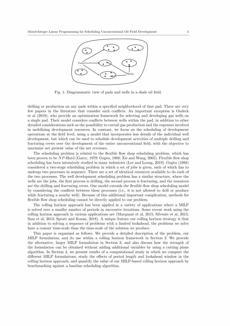
Fig. 1: Diagrammatic view of pads and wells in a shale oil field.
drilling or production on any pads within a specified neighborhood of that pad. There are veryfew papers in the literature that consider such conflicts. An important exception is Ondecket al (2019), who provide an optimization framework for selecting and developing gas wells ona single pad. Their model considers conflicts between wells within the pad, in addition to otherdetailed considerations such as the possibility to curtail gas production and the expenses involvedin mobilizing development resources. In contrast, we focus on the scheduling of developmentoperations at the field level, using a model that incorporates less details of the individual welldevelopment, but which can be used to schedule development activities of multiple drilling andfracturing crews over the development of the entire unconventional field, with the objective tomaximize net present value of the net revenues.
The scheduling problem is related to the flexible flow shop scheduling problem, which hasbeen proven to be NP -Hard (Garey, 1979; Gupta, 1988; Xie and Wang, 2005). Flexible flow shopscheduling has been intensively studied in many industries (Lee and Loong, 2019). Gupta (1988)considered a two-stage scheduling problem in which a set of jobs is given, each of which has toundergo two processes in sequence. There are a set of identical resources available to do each ofthe two processes. The well development scheduling problem has a similar structure, where thewells are the jobs, the first process is drilling, the second process is fracturing, and the resourcesare the drilling and fracturing crews. Our model extends the flexible flow shop scheduling modelby considering the conflicts between these processes (i.e., it is not allowed to drill or producewhile fracturing a nearby well). Because of this additional important complication, methods forflexible flow shop scheduling cannot be directly applied to our problem.
The rolling horizon approach has been applied in a variety of applications where a MILPis solved over a smaller number of periods in successive iterations. Some recent work using therolling horizon approach in various applications are (Marquant et al, 2015; Silvente et al, 2015;Sam et al, 2013; Spratt and Kozan, 2018). A unique feature our rolling horizon strategy is thatin addition to solving a sequence of problems with a limited lookahead, the problems we solvehave a coarser time-scale than the time-scale of the solution we produce.
This paper is organized as follows. We provide a detailed description of the problem, ourMILP formulation, and its use within a rolling horizon framework in Section 2. We providethe alternative, larger MILP formulation in Section 3, and also discuss how the strength ofthe formulation can be obtained without adding additional variables by using a cutting planealgorithm. In Section 4, we present results of a computational study in which we compare thedifferent MILP formulations, study the effects of period length and lookahead window in therolling horizon approach, and quantify the value of our MILP-based rolling horizon approach bybenchmarking against a baseline scheduling algorithm.
4 Soni et al.
2 Problem Description and Solution Approach
2.1 Problem Statement
We consider an oil field that has a collection of pads P to be developed as shown in Figure 1.A pad p ∈ P is a piece of land containing a number of wells. The first step in developing a padp ∈ P is drilling, which takes τdp days. The second step is fracturing which takes τfp days. Note
that we use (ˆ) to denote the time in days, whereas in section 2.3 we will use, e.g., τdp to representthe approximate number of periods to drill pad p for a given coarser time discretization. Drillingand fracturing operations have a fixed cost cdp and cfp associated with them, which are assumedto be charged at the beginning of the operation. The final steps in the development of a pad arecleaning and turning in line operations, but as these are typically done after fracturing withoutdelay and cause no conflicts with other operations, we do not consider them in our model.
A fixed number of drilling (nd) and fracturing (nf ) crews are available, so that at any point intime at most nd pads can be in the process of drilling and at most nf pads can be in the processof fracturing. At most one drilling crew or fracturing crew can be assigned to a pad. Moreover,each pad p is drilled and fractured in a single visit of drilling and fracturing crew respectively,without interruption.
A pad p starts producing oil after fracturing is complete. The amount of oil produced from apad in a period depends on the amount of time since the pad began fracturing, and is specifiedby a production curve αp, where αpk represents the amount of oil production from pad p duringday k after fracturing was started. Since production cannot occur while a pad is being fracturedand cleaned the production curve is zero for the initial periods until fracturing and cleaning arecomplete, then increases to the pad’s actual initial production level, and typically decreases overtime after that. The production curve of a pad is obtained by summing the production curves ofthe individual wells on the pad.
Since fracturing consists of pumping pressurized liquid into the well, as a safety and produc-tion protection measure, when fracturing occurs at a well on a pad, drilling and production atneighboring pads is stopped to prevent damage to equipment. For each pad p ∈ P the set Np ⊆ Prepresents the neighboring pads for which production and drilling are prohibited when pad p isbeing fractured. Although it is not necessary for our model, we assume the neighborhoods aresymmetric so that p ∈ Nq if and only if q ∈ Np for p, q ∈ P . If a pad that has completed fracturingis shut down due to fracturing at a neighboring well, we assume that the production profile ofthe pad still progresses to the next time period. Since the production rate curves are decreasing,when production resumes it will be at a lower rate. We let P oil denote the net revenue (price lessprocessing costs) per barrel of oil and assume it is known and fixed for the entire time horizonof the field development process. The problem is to determine the drilling and fracturing starttime of each pad in the field in order to maximize the net present value (NPV) of net revenuesobtained from the field over its production horizon, where NPV is calculated using an annualdiscount rate of iA. We let iD = 365
√iA + 1− 1 denote the equivalent daily discount rate.
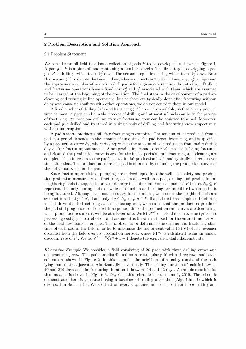
Illustrative Example We consider a field consisting of 20 pads with three drilling crews andone fracturing crew. The pads are distributed on a rectangular grid with three rows and sevencolumns as shown in Figure 2. In this example, the neighbors of a pad p consist of the padslying immediate adjacent to p horizontally or vertically. The drilling duration of pads is between40 and 210 days and the fracturing duration is between 14 and 42 days. A sample schedule forthis instance is shown in Figure 3. Day 0 in this schedule is set as Jan 1, 2019. The scheduledemonstrated here is generated using a baseline scheduling algorithm (Algorithm 2) which isdiscussed in Section 4.3. We see that on every day, there are no more than three drilling and
Mixed-Integer Linear Programming for Scheduling Unconventional Oil Field Development 5
Pad
Nbd. Pads
P1
P2 P3 P4 P5 P6
P7
P8
P9 P10 P11 P12 P13
P14
P15
P16 P17 P18 P19 P20
Fig. 2: Layout of pads in the illustrative example. The neighbors of pads P8, P11, and P7 areillustrated with dashed arrows.
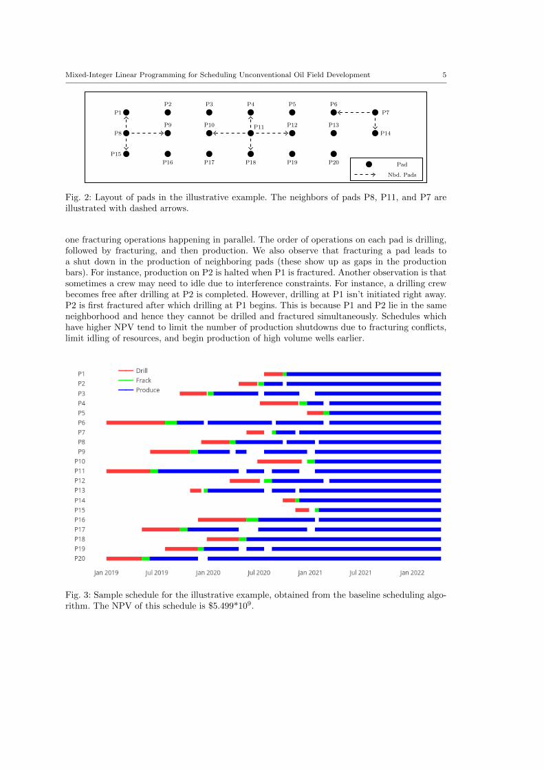
one fracturing operations happening in parallel. The order of operations on each pad is drilling,followed by fracturing, and then production. We also observe that fracturing a pad leads toa shut down in the production of neighboring pads (these show up as gaps in the productionbars). For instance, production on P2 is halted when P1 is fractured. Another observation is thatsometimes a crew may need to idle due to interference constraints. For instance, a drilling crewbecomes free after drilling at P2 is completed. However, drilling at P1 isn’t initiated right away.P2 is first fractured after which drilling at P1 begins. This is because P1 and P2 lie in the sameneighborhood and hence they cannot be drilled and fractured simultaneously. Schedules whichhave higher NPV tend to limit the number of production shutdowns due to fracturing conflicts,limit idling of resources, and begin production of high volume wells earlier.
Fig. 3: Sample schedule for the illustrative example, obtained from the baseline scheduling algo-rithm. The NPV of this schedule is $5.499*109.
6 Soni et al.
2.2 Coarse-Time Approximation
We formulate the pad drilling and fracturing scheduling problem as a MILP problem using adiscrete-time model consisting of a set of time periods T := {0, 1, . . . , |T |}. In order to obtaina more compact model, we assume a period consists of D days. For a pad p which takes τdpdays to drill, we approximate its drilling time in periods, τdp , by rounding τdp /D to the nearest
integer. Similarly, the fracturing duration in periods, τfp , is approximated by rounding τfp /D tothe nearest integer. The parameter D provides a trade-off in model accuracy and complexity. Alarger value of D leads to a problem with a shorter time horizon which is hence more compact,but also leads to more inaccuracy due to rounding.
Given the annual discount rate iA, the periodic discount rate i is given by the formula
i =N√iA + 1− 1,
where N represent the number of periods in a year.For a pad p ∈ P , the amount of oil produced in the tth period after fracturing was complete
is computed as
αpt =
(t+1)D−1∑k=tD
αpk. (1)
s If a pad begins production during the planning horizon, then our model needs to account for allproduction of the pad from the end of the planning horizon until the pad no longer produces. Todo so, for each pad p ∈ P and 0 ≤ t ≤ |T | − τfp , we define βpt to be the discounted total revenuefrom oil produced beyond the planning horizon if fracturing of pad p begins at time period t,where the revenue is discounted to period |T |. Specifically, βpt is computed as
βpt = P oilTMAXp∑
k=|T |−(t+τfp )
(1 + i)−kαpk. (2)
The oil that is produced within the planning horizon is accounted for differently because of thepossibility of production shut downs due to fracturing operations at neighboring pads, and thisis why βpt must be calculated separately for each possible fracturing start time t.
The notation used in our problem definition is summarized in Table 1.
2.3 MILP Formulation
The decision variables in the MILP model are as follows:
• xpt : Binary variable that takes the value 1 if drilling at pad p ∈ P starts at the beginning oftime period t ∈ T , 0 otherwise.
• ypt: Binary variable that takes the value 1 if fracturing at pad p ∈ P starts at the beginningof time period t ∈ T , 0 otherwise.
• xpt: Binary variable that takes the value 1 if drilling for pad p ∈ P has been completed bythe beginning of time period t ∈ T , 0 otherwise.
• ypt: Binary variable that takes the value 1 if fracturing for pad p ∈ P has been completed bythe beginning of time period t ∈ T , 0 otherwise.
• wpt: Binary variable that takes the value 1 if pad p ∈ P is in production mode in periodt ∈ T , 0 otherwise.
• vpt: Amount of oil produced from pad p ∈ P during period t ∈ T .
Mixed-Integer Linear Programming for Scheduling Unconventional Oil Field Development 7
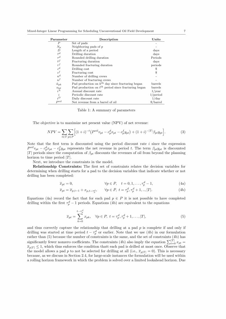
Parameter Description UnitsP Set of pads -Np Neighboring pads of p -D Length of a period daysτd Drilling duration daysτd Rounded drilling duration Periodsτf Fracturing duration daysτf Rounded fracturing duration periodscd Drilling cost $cf Fracturing cost $nd Number of drilling crews -nf Number of fracturing crews -αpk Pad production on kth day since fracturing began barrelsαpt Pad production on tth period since fracturing began barrelsiA Annual discount rate 1/yeari Periodic discount rate 1/periodiD Daily discount rate 1/dayP oil Net revenue from a barrel of oil $/barrel
Table 1: A summary of parameters
The objective is to maximize net present value (NPV) of net revenue:
NPV =∑t∈T
∑p∈P
[(1 + i)−t
(P oilvpt − cdpxpt − cfpypt
)+ (1 + i)−|T |βptypt
]. (3)
Note that the first term is discounted using the period discount rate i since the expressionP oilvpt − cdpxpt − cfpypt represents the net revenue in period t. The term βptypt is discounted|T | periods since the computation of βpt discounts the revenues of oil from beyond the planninghorizon to time period |T |.
Next, we introduce the constraints in the model.Relationship Constraints: The first set of constraints relates the decision variables for
determining when drilling starts for a pad to the decision variables that indicate whether or notdrilling has been completed:
xpt = 0, ∀p ∈ P, t = 0, 1, . . . , τdp − 1, (4a)
xpt = xp,t−1 + xp,t−τdp, ∀p ∈ P, t = τdp , τ
dp + 1, .., |T |. (4b)
Equations (4a) record the fact that for each pad p ∈ P it is not possible to have completeddrilling within the first τdp − 1 periods. Equations (4b) are equivalent to the equations
xpt =
t−τdp∑
k=0
xpk, ∀p ∈ P, t = τdp , τdp + 1, . . . , |T |, (5)
and thus correctly capture the relationship that drilling at a pad p is complete if and only ifdrilling was started at time period t − τdp or earlier. Note that we use (4b) in our formulationrather than (5) because the number of constraints is the same, and the set of constraints (4b) has
significantly fewer nonzero coefficients. The constraints (4b) also imply the equation∑|T |t=0 xpt =
xp|T | ≤ 1, which thus enforces the condition thatt each pad is drilled at most once. Observe thatthe model allows a pad p to not be selected for drilling at all (i.e., xp|T | = 0). This is necessarybecause, as we discuss in Section 2.4, for large-scale instances the formulation will be used withina rolling horizon framework in which the problem is solved over a limited lookahead horizon. Due
8 Soni et al.
to the limited length of the lookahead horizon it may note be feasible to drill all the wells withinthe horizon.
A similar set of constraints relates the decision variables for determining when fracturingstarts for a pad to the decision variables that indicate whether or not fracturing has been com-pleted:
ypt = 0, ∀p ∈ P, t = 0, 1, . . . , τfp − 1, (6a)
ypt = yp,t−1 + yp,t−τfp, ∀p ∈ P, t = τfp , τ
fp + 1, .., |T |. (6b)
Capacity Constraints: The following constraints ensure that the number of pads beingsimultaneously drilled or fractured doesn’t exceed the number of drilling or fracturing crewsavailable at any period:
∑p∈P
t∑k=(t−τd
p+1)+
xpk ≤ nd, ∀t ∈ T, (7)
∑p∈P
t∑k=(t−τf
p +1)+
ypk ≤ nf , ∀t ∈ T. (8)
Here we use the notation (z)+ = max{0, z} for any integer z. Note that a pad p ∈ P is beingdrilled at time t if it has begun drilling in one of the periods τdp before t, thus the expression onthe left-hand side of (7) computes the number of pads being drilled at time t, and similarly forfracturing in (8).
Precedence Constraints: We next consider constraints that enforce that drilling must bedone before fracturing. Specifically, the following constraints ensure that if drilling for a padp ∈ P has not yet been completed by a time t, then fracturing cannot be completed by timet+ τfp :
yp,t+τfp≤ xpt, ∀p ∈ P, t = 0, 1, ..., |T | − τfp . (9)
Similarly, production can occur only after a pad has completed fracturing. The following con-straint therefore enforces that if fracturing is not yet complete on a pad p ∈ P by time period t,then time period t cannot be a production period:
wpt ≤ ypt, ∀p ∈ P, t ∈ T. (10)
Operational Constraints: Since drilling must be done before fracturing, and a pad cannotbe producing until fracturing is complete we add the following constraints that prohibit a padfrom having more than one operation (drilling, fracturing, or producing) occur at any time periodt:
wpt +
t∑k=t−τd
p+1
xpk +
t∑k=t−τf
p +1
ypk ≤ 1, ∀p ∈ P, t = τdp , τdp + 1, ..., |T |. (11)
Vicinity Constraints: For each pad p and time period t, if any pad q ∈ Np is being fracturedat time t, then p cannot be in the process of drilling during that period, nor can it be producingduring that period:
wpt +
t∑k=(t−τd
p+1)+
xpk ≤ 1−t∑
k=(t−τfq +1)+
yqk, ∀p ∈ P, q ∈ Np, t ∈ T. (12)
Mixed-Integer Linear Programming for Scheduling Unconventional Oil Field Development 9
Oil Production Constraints: The volume of oil that can be produced from pad p in timeperiod t (vpt) is bounded above based on the production curve and when fracturing of the padbegan:
vpt ≤t−τf
p∑k=0
αp,t−kypk, ∀p ∈ P, t = τfp , τfp + 1, .., |T |. (13)
If ypk = 0 for all k ≤ t−τfp , then fracturing is not yet complete by time t and hence (13) correctly
records that no production can occur in period t. Otherwise, if ypk = 1 for some k ≤ t− τfp , then(13) bounds the production to not exceed αp,t−k, which is the limit in period t since in this casefracturing began t− k periods before period t.
In addition, the production amount from a pad must be zero if the pad is shut down due tofracturing at a neighboring pad. A shut down of pad p in time period t due to fracturing in aneighboring pad will cause wpt = 0 due to constraints (12). Thus the following constraint thenensures the volume produced is zero in this case:
vpt ≤ αpwpt, ∀p ∈ P, t ∈ T, (14)
where αp is an upper bound on the maximum possible production from pad p in a period (e.g.,αp = max{αpk : k ≥ 0}).
Note that when wpt = 1 for a pad p ∈ P in a time period t ∈ T , the production amountvpt will be exactly equal to the expression in the right-hand side of (13) due to the objectivefunction. We must use inequality in the constraint (13) in order to allow vpt = 0 in the case thatwpt = 0.
In summary, the MILP formulation is to maximize the objective (3), subject to the constraints(4), (6) - (14), and with binary restrictions on the decision variables xpt, ypt, xpt, ypt, wpt forp ∈ P, t ∈ T , and non-negativity on the oil production variables, vpt ≥ 0 for p ∈ P, t ∈ T . Werefer to this formulation as MILP1.
2.4 Rolling Horizon Implementation
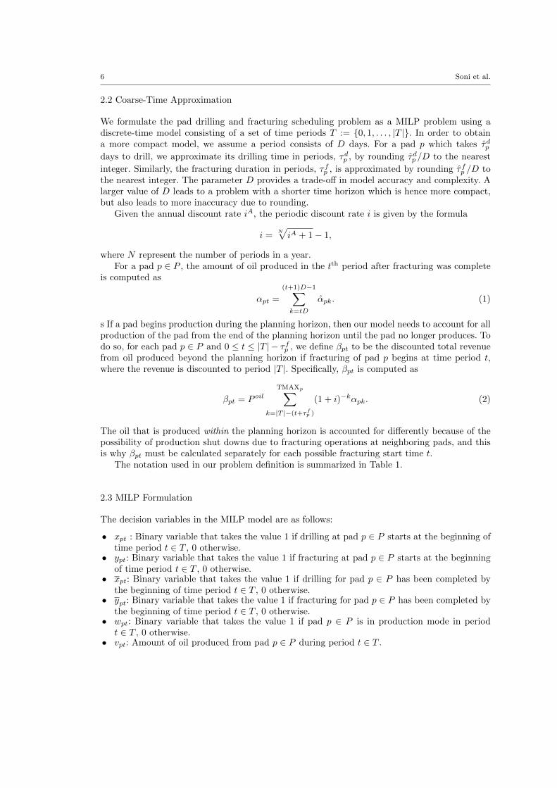
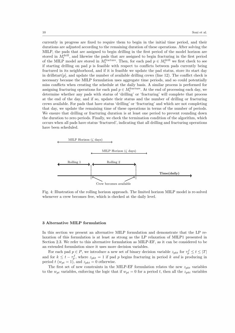
We next present a rolling horizon approach which is designed to obtain solutions for the problemfor significantly larger instances. The basic idea with a rolling horizon framework is to solve amodel over a limited planning horizon, fix the initial decisions, then move the window of theplanning horizon forward in time and repeat. We let ζ = |T |D be the number of days in theplanning horizon of the optimization model. In addition to limiting the planning horizon, we alsouse time periods of length D days to limit the size of the MILP formulation being solved at eachstep. However, the rolling forward is done at the daily level, so that in the end the algorithmproduces a schedule that is feasible to the problem using a daily time discretization. Figure 4illustrates the basic idea of the approach.
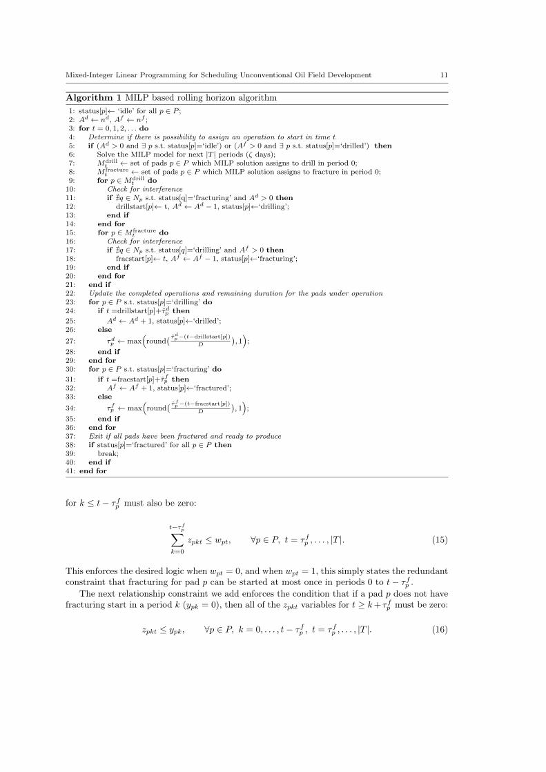
The details of the MILP-based rolling horizon approach are given in Algorithm 1. The statusof each pad is maintained throughout the algorithm, which is initialized as ‘idle’. The status ofa pad is updated to ‘drilling’ when it is in the process of drilling, and changes to ‘drilled’ afterdrilling is complete. When fracturing begins the status is updated to ‘fracturing’ and finally it isupdated to ‘fractured’ when that is complete, after which all operations for the pad are done. Thenumber of available drilling and fracturing crews at the current day is updated in the variablesAd and Af , respectively. At the beginning of processing each day, we first check to see if thereare any free drilling crews and pads that need to be drilled, or there are any free fracturing crewsand pads that need to be fractured. If so, the limited horizon, aggregate time-period MILP modelis solved (line 6). In this MILP, the decision variables for any drilling or fracturing operations
10 Soni et al.
currently in progress are fixed to require them to begin in the initial time period, and theirdurations are adjusted according to the remaining duration of these operations. After solving theMILP, the pads that are assigned to begin drilling in the first period of the model horizon arestored in Mdrill
t , and likewise the pads that are assigned to begin fracturing in the first periodof the MILP model are stored in M fracture
t . Then, for each pad p ∈ Mdrillt we first check to see
if starting drilling on pad p is feasible with respect to conflicts between pads currently beingfractured in its neighborhood, and if it is feasible we update the pad status, store its start dayin drillstart[p], and update the number of available drilling crews (line 12). The conflict check isnecessary because the MILP formulation uses aggregate time periods, and so could potentiallymiss conflicts when creating the schedule at the daily basis. A similar process is performed forassigning fracturing operations for each pad p ∈M fracture
t . At the end of processing each day, wedetermine whether any pads with status of ‘drilling’ or ‘fracturing’ will complete that processat the end of the day, and if so, update their status and the number of drilling or fracturingcrews available. For pads that have status ‘drilling’ or ‘fracturing’ and which are not completingthat day, we update the remaining time of these operations in terms of the number of periods.We ensure that drilling or fracturing duration is at least one period to prevent rounding downthe duration to zero periods. Finally, we check the termination condition of the algorithm, whichoccurs when all pads have status ‘fractured’, indicating that all drilling and fracturing operationshave been scheduled.
Time(daily)
Rolling 1 Rolling 2
MILP Horizon (ζ days)
MILP Horizon (ζ days)
Crew becomes available
Fig. 4: Illustration of the rolling horizon approach. The limited horizon MILP model is re-solvedwhenever a crew becomes free, which is checked at the daily level.
3 Alternative MILP formulation
In this section we present an alternative MILP formulation and demonstrate that the LP re-laxation of this formulation is at least as strong as the LP relaxation of MILP1 presented inSection 2.3. We refer to this alternative formulation as MILP-EF, as it can be considered to bean extended formulation since it uses more decision variables.
For each pad p ∈ P , we introduce a new set of binary decision variable zpkt for τfp ≤ t ≤ |T |and for k ≤ t − τfp , where zpkt = 1 if pad p begins fracturing in period k and is producing inperiod t (wpt = 1), and zpkt = 0 otherwise.
The first set of new constraints in the MILP-EF formulation relates the new zpkt variablesto the wpt variables, enforcing the logic that if wpt = 0 for a period t, then all the zpkt variables
Mixed-Integer Linear Programming for Scheduling Unconventional Oil Field Development 11
Algorithm 1 MILP based rolling horizon algorithm
1: status[p]← ‘idle’ for all p ∈ P ;2: Ad ← nd, Af ← nf ;3: for t = 0, 1, 2, . . . do4: Determine if there is possibility to assign an operation to start in time t5: if (Ad > 0 and ∃ p s.t. status[p]=‘idle’) or (Af > 0 and ∃ p s.t. status[p]=‘drilled’) then6: Solve the MILP model for next |T | periods (ζ days);7: Mdrill
t ← set of pads p ∈ P which MILP solution assigns to drill in period 0;8: M fracture
t ← set of pads p ∈ P which MILP solution assigns to fracture in period 0;9: for p ∈Mdrill
t do10: Check for interference11: if @q ∈ Np s.t. status[q]=‘fracturing’ and Ad > 0 then12: drillstart[p]← t, Ad ← Ad − 1, status[p]←‘drilling’;13: end if14: end for15: for p ∈M fracture
t do16: Check for interference17: if @q ∈ Np s.t. status[q]=‘drilling’ and Af > 0 then18: fracstart[p]← t, Af ← Af − 1, status[p]←‘fracturing’;19: end if20: end for21: end if22: Update the completed operations and remaining duration for the pads under operation23: for p ∈ P s.t. status[p]=‘drilling’ do24: if t =drillstart[p]+τdp then
25: Ad ← Ad + 1, status[p]←‘drilled’;26: else
27: τdp ← max(round
( τdp−(t−drillstart[p])
D
), 1
);
28: end if29: end for30: for p ∈ P s.t. status[p]=‘fracturing’ do
31: if t =fracstart[p]+τfp then32: Af ← Af + 1, status[p]←‘fractured’;33: else
34: τfp ← max(round
( τfp−(t−fracstart[p])
D
), 1
);
35: end if36: end for37: Exit if all pads have been fractured and ready to produce38: if status[p]=‘fractured’ for all p ∈ P then39: break;40: end if41: end for
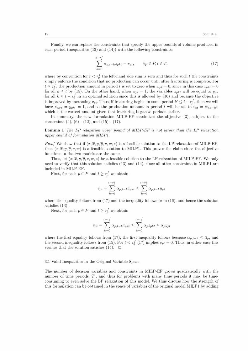
for k ≤ t− τfp must also be zero:
t−τfp∑
k=0
zpkt ≤ wpt, ∀p ∈ P, t = τfp , . . . , |T |. (15)
This enforces the desired logic when wpt = 0, and when wpt = 1, this simply states the redundantconstraint that fracturing for pad p can be started at most once in periods 0 to t− τfp .
The next relationship constraint we add enforces the condition that if a pad p does not havefracturing start in a period k (ypk = 0), then all of the zpkt variables for t ≥ k+ τfp must be zero:
zpkt ≤ ypk, ∀p ∈ P, k = 0, . . . , t− τfp , t = τfp , . . . , |T |. (16)
12 Soni et al.
Finally, we can replace the constraints that specify the upper bounds of volume produced ineach period (inequalities (13) and (14)) with the following constraints:
t−τfp∑
k=0
αp,t−kzpkt = vpt, ∀p ∈ P, t ∈ T, (17)
where by convention for t < τfp the left-hand side sum is zero and thus for such t the constraintssimply enforce the condition that no production can occur until after fracturing is complete. Fort ≥ τfp , the production amount in period t is set to zero when wpt = 0, since in this case zpkt = 0for all k ≤ t by (15). On the other hand, when wpt = 1, the variables zpkt will be equal to ypkfor all k ≤ t− τfp in an optimal solution since this is allowed by (16) and because the objective
is improved by increasing vpt. Thus, if fracturing begins in some period k′ ≤ t− τfp , then we willhave zpk′t = ypk′ = 1, and so the production amount in period t will be set to vpt = αp,t−k′ ,which is the correct amount given that fracturing began k′ periods earlier.
In summary, the new formulation MILP-EF maximizes the objective (3), subject to theconstraints (4), (6) - (12), and (15) - (17).
Lemma 1 The LP relaxation upper bound of MILP-EF is not larger than the LP relaxationupper bound of formulation MILP1.
Proof We show that if (x, x, y, y, v, w, z) is a feasible solution to the LP relaxation of MILP-EF,then (x, x, y, y, v, w) is a feasible solution to MILP1. This proves the claim since the objectivefunctions in the two models are the same.
Thus, let (x, x, y, y, v, w, z) be a feasible solution to the LP relaxation of MILP-EF. We onlyneed to verify that this solution satisfies (13) and (14), since all other constraints in MILP1 areincluded in MILP-EF.
First, for each p ∈ P and t ≥ τfp we obtain
vpt =
t−τfp∑
k=0
αp,t−kzpkt ≤t−τf
p∑k=0
αp,t−kypk
where the equality follows from (17) and the inequality follows from (16), and hence the solutionsatisfies (13).
Next, for each p ∈ P and t ≥ τfp we obtain
vpt =
t−τfp∑
k=0
αp,t−kzpkt ≤t−τf
p∑k=0
αpzpkt ≤ αpypt
where the first equality follows from (17), the first inequality follows because αp,t−k ≤ αp, andthe second inequality follows from (15). For t < τfp (17) implies vpt = 0. Thus, in either case thisverifies that the solution satisfies (14). ut
3.1 Valid Inequalities in the Original Variable Space
The number of decision variables and constraints in MILP-EF grows quadratically with thenumber of time periods |T |, and thus for problems with many time periods it may be time-consuming to even solve the LP relaxation of this model. We thus discuss how the strength ofthis formulation can be obtained in the space of variables of the original model MILP1 by adding
Mixed-Integer Linear Programming for Scheduling Unconventional Oil Field Development 13
valid inequalities as cuts to the LP relaxation. One possible implementation of this would be toadd these valid inequalities at the initial LP relaxation before starting the branch-and-boundprocess for solving MILP1.
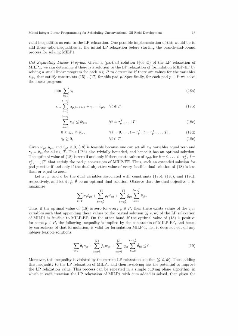
Cut Separating Linear Program. Given a (partial) solution (y, v, w) of the LP relaxation ofMILP1, we can determine if there is a solution to the LP relaxation of formulation MILP-EF bysolving a small linear program for each p ∈ P to determine if there are values for the variablesztkp that satisfy constraints (15) - (17) for this pad p. Specifically, for each pad p ∈ P we solvethe linear program:
min∑k∈T
γt (18a)
s.t.
t−τfp∑
k=0
αp,t−kztk + γt = vpt, ∀t ∈ T, (18b)
t−τfp∑
k=0
ztk ≤ wpt, ∀t = τfp , . . . , |T |, (18c)
0 ≤ ztk ≤ ypt, ∀k = 0, . . . , t− τfp , t = τfp , . . . , |T |, (18d)
γt ≥ 0, ∀t ∈ T. (18e)
Given wpt, ypt, and vpt ≥ 0, (18) is feasible because one can set all ztk variables equal zero andγt = vpt for all t ∈ T . This LP is also trivially bounded, and hence it has an optimal solution.The optimal value of (18) is zero if and only if there exists values of zptk for k = 0, . . . , t−τfp , t =
τfp , . . . , |T | that satisfy the pad p constraints of MILP-EF. Thus, such an extended solution forpad p exists if and only if the dual objective value of every feasible dual solution of (18) is lessthan or equal to zero.
Let π, ρ, and θ be the dual variables associated with constraints (18b), (18c), and (18d),
respectively, and let π, ρ, θ be an optimal dual solution. Observe that the dual objective is tomaximize ∑
t∈Tπtvpt +
|T |∑t=τf
p
ρtwpt +
|T |∑t=τf
p
ypt
t−τfp∑
k=0
θtk.
Thus, if the optimal value of (18) is zero for every p ∈ P , then there exists values of the zptkvariables such that appending these values to the partial solution (y, v, w) of the LP relaxationof MILP1 is feasible to MILP-EF. On the other hand, if the optimal value of (18) is positivefor some p ∈ P , the following inequality is implied by the constraints of MILP-EF, and henceby correctness of that formulation, is valid for formulation MILP-1, i.e., it does not cut off anyinteger feasible solutions:
∑t∈T
πtvpt +
|T |∑t=τf
p
ρtwpt +
|T |∑t=τf
p
ypt
t−τfp∑
k=0
θtk ≤ 0. (19)
Moreover, this inequality is violated by the current LP relaxation solution (y, v, w). Thus, addingthis inequality to the LP relaxation of MILP1 and then re-solving has the potential to improvethe LP relaxation value. This process can be repeated in a simple cutting plane algorithm, inwhich in each iteration the LP relaxation of MILP1 with cuts added is solved, then given the
14 Soni et al.
solution the cut separating linear programs (18) are solved for each p ∈ P , and then cuts ofthe form (19) are added when violated. If the process continues until no more violated cuts arefound, the resulting LP relaxation value will be equal to the LP relaxation value of MILP-EF.
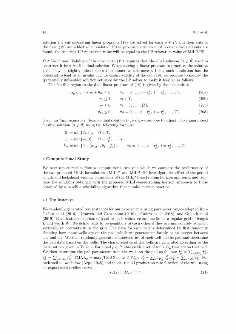
Cut Validation. Validity of the inequality (19) requires that the dual solution (π, ρ, θ) used toconstruct it be a feasible dual solution. When solving a linear program in practice, the solutiongiven may be slightly infeasible (within numerical tolerances). Using such a solution has thepotential to lead to an invalid cut. To ensure validity of the cut (19), we propose to modify the(potentially infeasible) solution returned by the LP solver to make it feasible as follows.
The feasible region to the dual linear program of (18) is given by the inequalities
αp,t−kπt + ρt + θtk ≤ 0, ∀k = 0, . . . , t− τfp , t = τfp , . . . , |T |, (20a)
πt ≤ 1, ∀t ∈ T, (20b)
ρt ≤ 0, ∀t = τfp , . . . , |T |, (20c)
θkt ≤ 0, ∀k = 0, . . . , t− τfp , t = τfp , . . . , |T |. (20d)
Given an “approximately” feasible dual solution (π, ρ, θ), we propose to adjust it to a guaranteedfeasible solution (π, ρ, θ) using the following formulae:
πt = min{πt, 1}, ∀t ∈ T,ρt = min{ρt, 0}, ∀t = τfp , . . . , |T |,θtk = min{0,−(αp,t−kπt + ρt)}, ∀k = 0, . . . , t− τfp , t = τfp , . . . , |T |.
4 Computational Study
We next report results from a computational study in which we compare the performance ofthe two proposed MILP formulations, MILP1 and MILP-EF, investigate the effect of the periodlength and lookahead window parameters of the MILP-based rolling horizon approach, and com-pare the solutions obtained with the proposed MILP-based rolling horizon approach to thoseobtained by a baseline scheduling algorithm that mimics current practice.
4.1 Test Instances
We randomly generated test instances for our experiments using parameter ranges adopted fromCafaro et al (2016), Drouven and Grossmann (2016) , Cafaro et al (2018), and Ondeck et al(2019). Each instance consists of a set of pads which we assume lie on a regular grid of lengthL and width W . We define pads to be neighbors of each other if they are immediately adjacentvertically or horizontally in the grid. The data for each pad is determined by first randomlychoosing how many wells are on the pad, which we generate uniformly as an integer betweenone and six. We then randomly generate characteristics of each well on the pad and determinethe pad data based on the wells. The characteristics of the wells are generated according to thedistributions given in Table 2. For a pad p ∈ P , this yields a set of wellsWp that are on that pad.We then determine the pad parameters from the wells on the pad as follows: τdp =
∑w∈Wp
τdw,
τfp =∑w∈Wp
τfw, TMAXp = max{TMAXw : w ∈ Wp}, cdp =∑w∈Wp
cdw, cfp =∑w∈Wp
cfw. For
each well w, we follow (Arps, 1945) and model the oil production rate function of the well usingan exponential decline curve
λw(s) = Mwe−aws, (21)
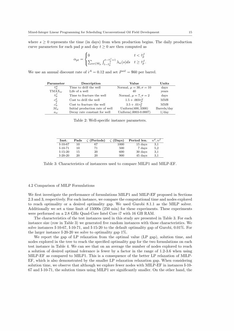
Mixed-Integer Linear Programming for Scheduling Unconventional Oil Field Development 15
where s ≥ 0 represents the time (in days) from when production begins. The daily productioncurve parameters for each pad p and day t ≥ 0 are then computed as
αpt =
0 t < τfp∑w∈Wp
∫ t−τfp +1
t−τfp
λw(s)ds t ≥ τfp .
We use an annual discount rate of iA = 0.12 and set P oil = $60 per barrel.
Parameter Description Value Units
τdw Time to drill the well Normal, µ = 30, σ = 10 daysTMAXw Life of a well 40 years
τfw Time to fracture the well Normal, µ = 7, σ = 2 days
cdw Cost to drill the well 1.5 + .003τdp MM$
cfw Cost to fracture the well 3.5 + .01τdp MM$Mw Initial production rate of well Uniform(400, 3300) Barrels/dayaw Decay rate constant for well Uniform(.0003-0.0007) 1/day
Table 2: Well-specific instance parameters.
Inst. Pads ζ (Periods) ζ (Days) Period len. nd, nf
I-10-67 10 67 1000 15 days 3,1I-10-71 10 71 500 7 days 5,2I-15-20 15 20 600 30 days 3,1I-20-20 20 20 900 45 days 3,1
Table 3: Characteristics of instancees used to compare MILP1 and MILP-EF.
4.2 Comparison of MILP Formulations
We first investigate the performance of formulations MILP1 and MILP-EF proposed in Sections2.3 and 3, respectively. For each instance, we compare the computational time and nodes exploredto reach optimality or a desired optimality gap. We used Gurobi 8.1.1 as the MILP solver.Additionally we set a time limit of 15000s (250 min) for these experiments. These experimentswere performed on a 2.8 GHz Quad-Core Intel Core i7 with 16 GB RAM.
The characteristics of the test instances used in this study are presented in Table 3. For eachinstance size (row in Table 3) we generated five random instances with those characteristics. Wesolve instances I-10-67, I-10-71, and I-15-20 to the default optimality gap of Gurobi, 0.01%. Forthe larger instance I-20-20 we solve to optimality gap 1%.
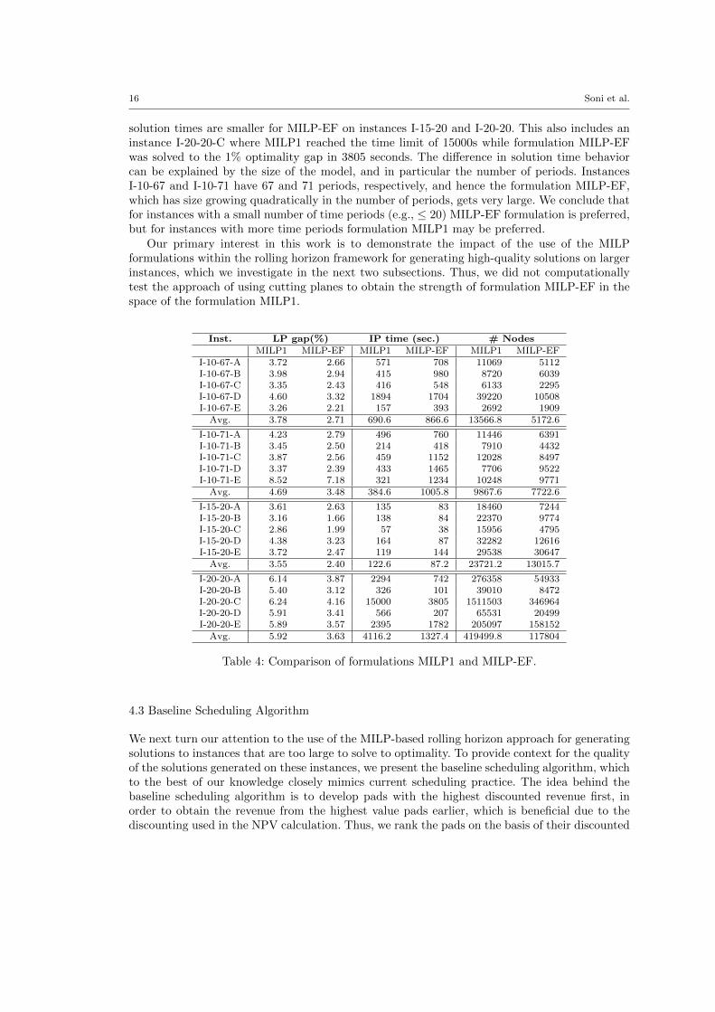
We report the gap of LP relaxation from the optimal value (LP gap), solution time, andnodes explored in the tree to reach the specified optimality gap for the two formulations on eachtest instance in Table 4. We can see that on an average the number of nodes explored to reacha solution of desired optimal tolerance is fewer by a factor in the range of 1.2-3.6 when usingMILP-EF as compared to MILP1. This is a consequence of the better LP relaxation of MILP-EF, which is also demonstrated by the smaller LP relaxation relaxation gap. When consideringsolution time, we observe that although we explore fewer nodes with MILP-EF in instances I-10-67 and I-10-71, the solution times using MILP1 are significantly smaller. On the other hand, the
16 Soni et al.
solution times are smaller for MILP-EF on instances I-15-20 and I-20-20. This also includes aninstance I-20-20-C where MILP1 reached the time limit of 15000s while formulation MILP-EFwas solved to the 1% optimality gap in 3805 seconds. The difference in solution time behaviorcan be explained by the size of the model, and in particular the number of periods. InstancesI-10-67 and I-10-71 have 67 and 71 periods, respectively, and hence the formulation MILP-EF,which has size growing quadratically in the number of periods, gets very large. We conclude thatfor instances with a small number of time periods (e.g., ≤ 20) MILP-EF formulation is preferred,but for instances with more time periods formulation MILP1 may be preferred.
Our primary interest in this work is to demonstrate the impact of the use of the MILPformulations within the rolling horizon framework for generating high-quality solutions on largerinstances, which we investigate in the next two subsections. Thus, we did not computationallytest the approach of using cutting planes to obtain the strength of formulation MILP-EF in thespace of the formulation MILP1.
Inst. LP gap(%) IP time (sec.) # NodesMILP1 MILP-EF MILP1 MILP-EF MILP1 MILP-EF
I-10-67-A 3.72 2.66 571 708 11069 5112I-10-67-B 3.98 2.94 415 980 8720 6039I-10-67-C 3.35 2.43 416 548 6133 2295I-10-67-D 4.60 3.32 1894 1704 39220 10508I-10-67-E 3.26 2.21 157 393 2692 1909
Avg. 3.78 2.71 690.6 866.6 13566.8 5172.6
I-10-71-A 4.23 2.79 496 760 11446 6391I-10-71-B 3.45 2.50 214 418 7910 4432I-10-71-C 3.87 2.56 459 1152 12028 8497I-10-71-D 3.37 2.39 433 1465 7706 9522I-10-71-E 8.52 7.18 321 1234 10248 9771
Avg. 4.69 3.48 384.6 1005.8 9867.6 7722.6
I-15-20-A 3.61 2.63 135 83 18460 7244I-15-20-B 3.16 1.66 138 84 22370 9774I-15-20-C 2.86 1.99 57 38 15956 4795I-15-20-D 4.38 3.23 164 87 32282 12616I-15-20-E 3.72 2.47 119 144 29538 30647
Avg. 3.55 2.40 122.6 87.2 23721.2 13015.7
I-20-20-A 6.14 3.87 2294 742 276358 54933I-20-20-B 5.40 3.12 326 101 39010 8472I-20-20-C 6.24 4.16 15000 3805 1511503 346964I-20-20-D 5.91 3.41 566 207 65531 20499I-20-20-E 5.89 3.57 2395 1782 205097 158152
Avg. 5.92 3.63 4116.2 1327.4 419499.8 117804
Table 4: Comparison of formulations MILP1 and MILP-EF.
4.3 Baseline Scheduling Algorithm
We next turn our attention to the use of the MILP-based rolling horizon approach for generatingsolutions to instances that are too large to solve to optimality. To provide context for the qualityof the solutions generated on these instances, we present the baseline scheduling algorithm, whichto the best of our knowledge closely mimics current scheduling practice. The idea behind thebaseline scheduling algorithm is to develop pads with the highest discounted revenue first, inorder to obtain the revenue from the highest value pads earlier, which is beneficial due to thediscounting used in the NPV calculation. Thus, we rank the pads on the basis of their discounted
Mixed-Integer Linear Programming for Scheduling Unconventional Oil Field Development 17
total revenue, which is computed in (2) as βp,|T |−τfp
. The operations are then scheduled by
prioritizing the pads with highest discounted volume production first, while ensuring that wedon’t violate any precedence, capacity, operational and conflict constraints.
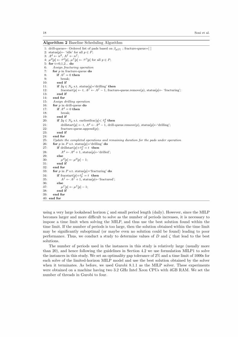
The details of the baseline scheduling algorithm are given in Algorithm 2. We create a drill-queue of the pads, ordered highest to lowest by discounted revenue. Pads are added to thefracture-queue (line 20) after their drilling operation is initiated. Note that the order in the twoqueues may be different as drilling operations may not always start in the preferred order due topossible delays due arising from conflicts. In the algorithm each pad is initialized with the ‘idle’status. We update the status of each pad as it goes through different stages of the developmentcycle, i.e., {‘idle’, ‘drilling’, ‘drilled’, ‘fracturing’, ‘fractured’ }. The variables Ad and Af keeptrack of the number of free drilling and fracturing crews available at each point in time. Ad
and Af are initialized with nd and nf as all crews are free at t = 0. Similarly, the variablesµd[p] and µf [p] are used to keep track of the remaining drilling and fracturing duration of eachpad p. These are initialized with the actual drilling and fracturing duration (τd[p] and τf [p]).Algorithm 2 proceeds by considering each day in the planning horizon in sequence. For eachday, we first assign fracturing operations (lines 6-14) and then drilling operations (lines 15-24)to start that day. Fracturing is prioritized over drilling in case there is a conflict between eitherstarting drilling or fracturing on two neighboring pads. Fracturing is prioritized because once itis complete the pad can begin production and revenue is generated. Fracturing operations areinitiated in preference order of the fracture-queue. Fracturing is initiated at the next pad in thequeue if there is a free fracturing crew, drilling is complete, and initiating fracturing on the givenpad doesn’t violate any interference constraints (lines 11-13). If all these conditions hold true,fracturing is started and we store the fracturing start day for the pad in ‘fracstart’, reduce thenumber of fracturing crews available (Af ) by one, remove the pad from the fracture queue, andupdate the status of pad to ‘fracturing’ (line 12). If a pad is not assigned for fracturing, but afracturing crew is still available, the next pad in the queue is considered, and so on until eitherthe full queue has been checked or there are no available fracturing crews. Drilling operationsare initiated in a similar way (lines 15-24). However, when initiating drilling operations we checkadditional conditions in order to avoid creating conflicts with upcoming fracturing operations(line 20). In particular, we check each neighboring pad q to see if it is currently being fractured(status[p]=‘fracturing’), is ready to be fractured(status[q]=‘drilled’), or there is a possibility thatit may begin fracturing before the drilling operation on pad p under consideration would becompleted (and hence starting drilling on this pad may delay fracturing pad q). To perform thischeck, we define the values ‘earlieststart[q]’ for q ∈ P as follows:
earlieststart[q] =
0, if status[q] = ‘fracturing’ or status[q] = ‘drilled’,
+∞, if status[p] = ‘idle’ or status[q] = ‘fractured’,∑ij=1 µ
f [qj ]/nf , if q = qi ∈ fracture-queue = [q1, q2, . . . , qk].
At the end of processing each day, we determine whether any pads with status of ‘drilling’ or‘fracturing’ will complete that process at the end of the day, and if so update their status and thenumber of drilling and fracturing crews available. For pads with status ‘drilling’ or ‘fracturing’and which are not completing that day, we update the remaining time of these operations (lines25-39).
4.4 Parameter Study for MILP+Rolling Horizon Approach
We next study the effect of the period length (D) and lookahead horizon (ζ) parameters in theMILP-based rolling horizon framework. Intuitively, one would expect to obtain the best solutions
18 Soni et al.
Algorithm 2 Baseline Scheduling Algorithm
1: drill-queue← Ordered list of pads based on βp|T | ; fracture-queue=[ ]2: status[p]← ‘idle’ for all p ∈ P ;3: Ad ← nd, Af ← nf ;4: µd[p]← τd[p], µf [p]← τf [p] for all p ∈ P ;5: for t=0,1,2... do6: Assign fracturing operation7: for p in fracture-queue do8: if Af = 0 then9: break;10: end if11: if @q ∈ Np s.t. status[q]=‘drilling’ then12: fracstart[p]← t, Af ← Af − 1, fracture-queue.remove(p), status[p]← ‘fracturing’;13: end if14: end for15: Assign drilling operation16: for p in drill-queue do17: if Ad = 0 then18: break;19: end if20: if @q ∈ Np s.t. earliestfrac[q]< τdp then
21: drillstart[p]← t, Ad ← Ad − 1, drill-queue.remove(p), status[p]←‘drilling’;22: fracture-queue.append(p);23: end if24: end for25: Update the completed operations and remaining duration for the pads under operation26: for p in P s.t. status[p]=‘drilling’ do27: if drillstart[p]+τdp = t then
28: Ad ← Ad + 1, status[p]←‘drilled’;29: else30: µd[p]← µd[p]− 1;31: end if32: end for33: for p in P s.t. status[p]=‘fracturing’ do
34: if fracstart[p]+τfp = t then35: Af ← Af + 1, status[p]←‘fractured’;36: else37: µf [p]← µf [p]− 1;38: end if39: end for40: end for
using a very large lookahead horizon ζ and small period length (daily). However, since the MILPbecomes larger and more difficult to solve as the number of periods increases, it is necessary toimpose a time limit when solving the MILP, and thus use the best solution found within thetime limit. If the number of periods is too large, then the solution obtained within the time limitmay be significantly suboptimal (or maybe even no solution could be found) leading to poorperformance. Thus, we conduct a study to determine values of D and ζ that lead to the bestsolutions.
The number of periods used in the instances in this study is relatively large (usually morethan 20), and hence following the guidelines in Section 4.2 we use formulation MILP1 to solvethe instances in this study. We set an optimality gap tolerance of 2% and a time limit of 1000s foreach solve of the limited-horizon MILP model and use the best solution obtained by the solverwhen it terminates. As before, we used Gurobi 8.1.1 as the MILP solver. These experimentswere obtained on a machine having two 3.2 GHz Intel Xeon CPUs with 4GB RAM. We set thenumber of threads in Gurobi to four.
Mixed-Integer Linear Programming for Scheduling Unconventional Oil Field Development 19
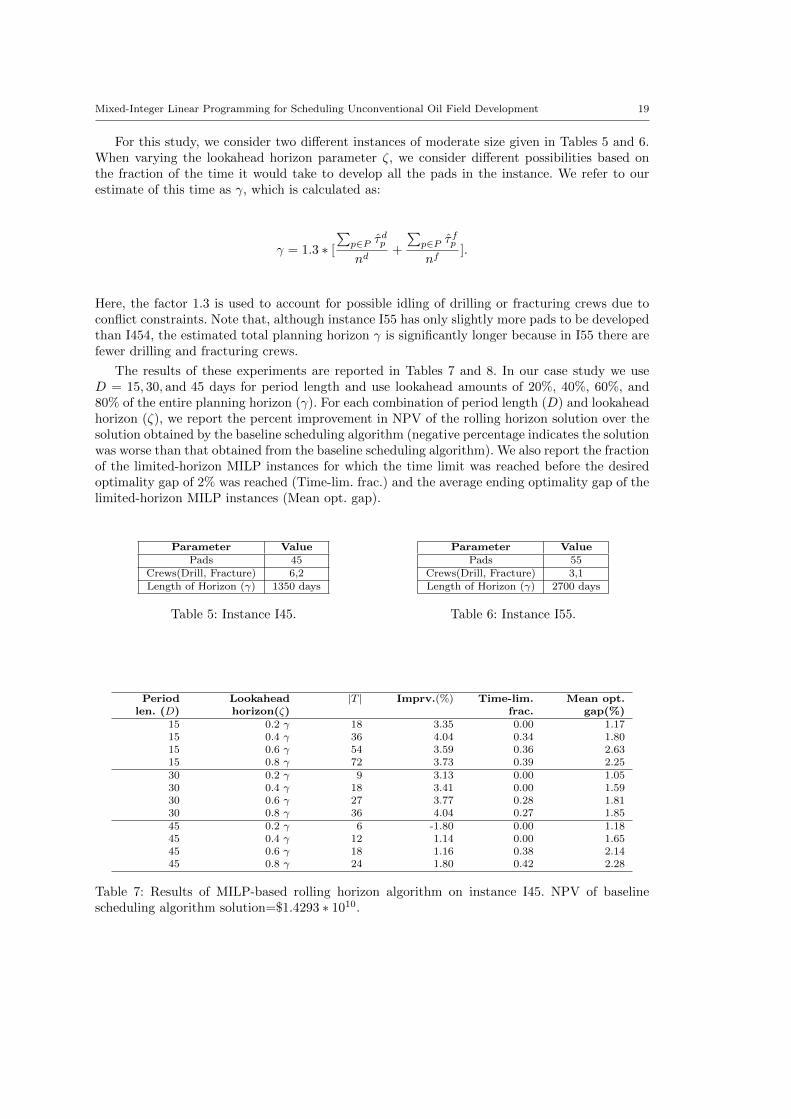
For this study, we consider two different instances of moderate size given in Tables 5 and 6.When varying the lookahead horizon parameter ζ, we consider different possibilities based onthe fraction of the time it would take to develop all the pads in the instance. We refer to ourestimate of this time as γ, which is calculated as:
γ = 1.3 ∗ [
∑p∈P τ
dp
nd+
∑p∈P τ
fp
nf].
Here, the factor 1.3 is used to account for possible idling of drilling or fracturing crews due toconflict constraints. Note that, although instance I55 has only slightly more pads to be developedthan I454, the estimated total planning horizon γ is significantly longer because in I55 there arefewer drilling and fracturing crews.
The results of these experiments are reported in Tables 7 and 8. In our case study we useD = 15, 30, and 45 days for period length and use lookahead amounts of 20%, 40%, 60%, and80% of the entire planning horizon (γ). For each combination of period length (D) and lookaheadhorizon (ζ), we report the percent improvement in NPV of the rolling horizon solution over thesolution obtained by the baseline scheduling algorithm (negative percentage indicates the solutionwas worse than that obtained from the baseline scheduling algorithm). We also report the fractionof the limited-horizon MILP instances for which the time limit was reached before the desiredoptimality gap of 2% was reached (Time-lim. frac.) and the average ending optimality gap of thelimited-horizon MILP instances (Mean opt. gap).
Parameter ValuePads 45
Crews(Drill, Fracture) 6,2Length of Horizon (γ) 1350 days
Table 5: Instance I45.
Parameter ValuePads 55
Crews(Drill, Fracture) 3,1Length of Horizon (γ) 2700 days
Table 6: Instance I55.
Periodlen. (D)
Lookaheadhorizon(ζ)
|T | Imprv.(%) Time-lim.frac.
Mean opt.gap(%)
15 0.2 γ 18 3.35 0.00 1.1715 0.4 γ 36 4.04 0.34 1.8015 0.6 γ 54 3.59 0.36 2.6315 0.8 γ 72 3.73 0.39 2.2530 0.2 γ 9 3.13 0.00 1.0530 0.4 γ 18 3.41 0.00 1.5930 0.6 γ 27 3.77 0.28 1.8130 0.8 γ 36 4.04 0.27 1.8545 0.2 γ 6 -1.80 0.00 1.1845 0.4 γ 12 1.14 0.00 1.6545 0.6 γ 18 1.16 0.38 2.1445 0.8 γ 24 1.80 0.42 2.28
Table 7: Results of MILP-based rolling horizon algorithm on instance I45. NPV of baselinescheduling algorithm solution=$1.4293 ∗ 1010.
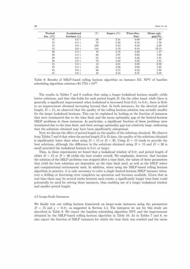
20 Soni et al.
Periodlen. (D)
Lookaheadhorizon (ζ)
|T | Imprv.(%) Time-lim.frac.
Mean opt.gap(%)
15 0.2 γ 36 5.21 0.00 1.4815 0.4 γ 72 5.30 0.16 1.7915 0.6 γ 108 5.24 0.45 2.2915 0.8 γ 144 5.19 0.44 18.1330 0.2 γ 18 2.78 0.00 1.4730 0.4 γ 36 4.97 0.03 1.6830 0.6 γ 54 5.10 0.30 1.8130 0.8 γ 72 5.22 0.29 1.9545 0.2 γ 12 2.61 0.00 0.9045 0.4 γ 24 3.56 0.00 1.6345 0.6 γ 36 3.15 0.34 1.8945 0.8 γ 48 3.54 0.37 2.20
Table 8: Results of MILP-based rolling horizon algorithm on instance I55. NPV of baselinescheduling algorithm solution=$1.7721 ∗ 1010.
The results in Tables 7 and 8 confirm that using a longer lookahead horizon usually yieldsbetter solutions, and that this holds for each period length D. On the other hand, while there isgenerally a significant improvement when lookahead is increased from 0.2γ to 0.4γ, there is littleto no improvement obtained increasing beyond that. In both instances, for the shortest periodlength, D = 15, we observed that the quality of the rolling horizon solution was actually smallerfor the larger lookahead horizons. This can be explained by looking at the fraction of instancesthat were terminated due to the time limit and the mean optimality gap of the limited-horizonMILP problems in these instances. In particular, a significant fraction of these problems wereterminated due to the time limit, and their average optimality gap was relatively large, indicatingthat the solutions obtained may have been significantly suboptimal.
Next we discuss the effect of period length on the quality of the solutions obtained. We observefrom Tables 7 and 8 that when the period lengthD is 45 days, the quality of the solutions obtainedis significantly lower than when using D = 15 or D = 30. Using D = 15 tends to provide thebest solutions, although the difference in the solutions obtained using D = 15 and D = 30 issmall provided the lookahead horizon is 0.4γ or larger.
Thus, in these experiments we found that a lookahead window of 0.4γ and period length ofeither D = 15 or D = 30 yields the best results overall. We emphasize, however, that becausethe solution of the MILP problems was stopped after a time limit, the values of these parametersthat yield the best solutions are dependent on the time limit used, as well as the MILP solverand computational environment used. In addition, when using the MILP-based rolling horizonalgorithm in practice, it is only necessary to solve a single limited-horizon MILP instance when-ever a drilling or fracturing crew completes an operation and becomes available. Given that inreal time there may be several weeks between such events, a significantly longer time limit couldpotentially be used for solving these instances, thus enabling use of a longer lookahead windowand smaller period length.
4.5 Large-Scale Instances
We finally test our rolling horizon framework on larger-scale instances using the parametersD = 15 and ζ = 0.4γ, as suggested in Section 4.4. The instances we use for this study aredescribed in Table 9. We report the baseline scheduling algorithm NPV and the improvementobtained by the MILP-based rolling horizon algorithm in Table 10. As in Tables 7 and 8, wealso report the fraction of MILP instances for which the time limit was reached and the mean
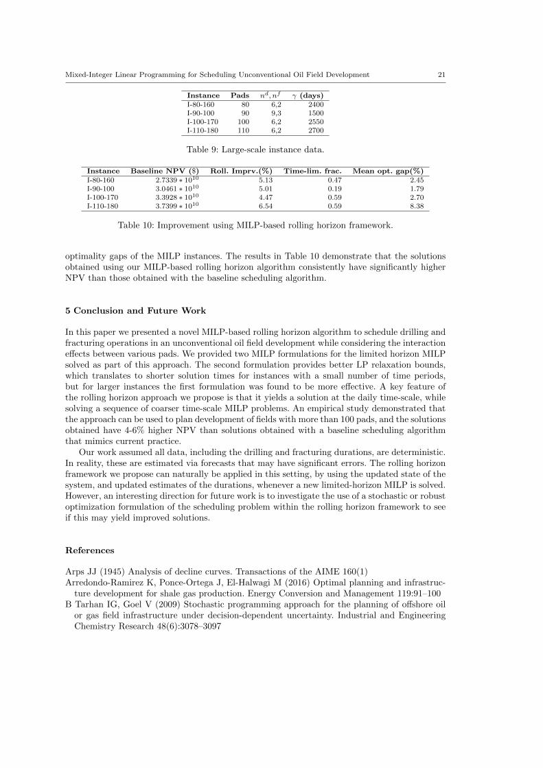
Mixed-Integer Linear Programming for Scheduling Unconventional Oil Field Development 21
Instance Pads nd, nf γ (days)I-80-160 80 6,2 2400I-90-100 90 9,3 1500I-100-170 100 6,2 2550I-110-180 110 6,2 2700
Table 9: Large-scale instance data.
Instance Baseline NPV ($) Roll. Imprv.(%) Time-lim. frac. Mean opt. gap(%)I-80-160 2.7339 ∗ 1010 5.13 0.47 2.45I-90-100 3.0461 ∗ 1010 5.01 0.19 1.79I-100-170 3.3928 ∗ 1010 4.47 0.59 2.70I-110-180 3.7399 ∗ 1010 6.54 0.59 8.38
Table 10: Improvement using MILP-based rolling horizon framework.
optimality gaps of the MILP instances. The results in Table 10 demonstrate that the solutionsobtained using our MILP-based rolling horizon algorithm consistently have significantly higherNPV than those obtained with the baseline scheduling algorithm.
5 Conclusion and Future Work
In this paper we presented a novel MILP-based rolling horizon algorithm to schedule drilling andfracturing operations in an unconventional oil field development while considering the interactioneffects between various pads. We provided two MILP formulations for the limited horizon MILPsolved as part of this approach. The second formulation provides better LP relaxation bounds,which translates to shorter solution times for instances with a small number of time periods,but for larger instances the first formulation was found to be more effective. A key feature ofthe rolling horizon approach we propose is that it yields a solution at the daily time-scale, whilesolving a sequence of coarser time-scale MILP problems. An empirical study demonstrated thatthe approach can be used to plan development of fields with more than 100 pads, and the solutionsobtained have 4-6% higher NPV than solutions obtained with a baseline scheduling algorithmthat mimics current practice.
Our work assumed all data, including the drilling and fracturing durations, are deterministic.In reality, these are estimated via forecasts that may have significant errors. The rolling horizonframework we propose can naturally be applied in this setting, by using the updated state of thesystem, and updated estimates of the durations, whenever a new limited-horizon MILP is solved.However, an interesting direction for future work is to investigate the use of a stochastic or robustoptimization formulation of the scheduling problem within the rolling horizon framework to seeif this may yield improved solutions.
References
Arps JJ (1945) Analysis of decline curves. Transactions of the AIME 160(1)Arredondo-Ramirez K, Ponce-Ortega J, El-Halwagi M (2016) Optimal planning and infrastruc-
ture development for shale gas production. Energy Conversion and Management 119:91–100B Tarhan IG, Goel V (2009) Stochastic programming approach for the planning of offshore oil
or gas field infrastructure under decision-dependent uncertainty. Industrial and EngineeringChemistry Research 48(6):3078–3097
22 Soni et al.
Cafaro C, Grossmann I (2014) Strategic planning, design, and development of the shale gassupplychain network. AIChE Journal 60:2122–2142
Cafaro C, Drouven M, E GI (2016) Optimization models for planning shale gas well refracturetreatments. AIChE Journal 62:4297–4307
Cafaro DC, Drouven M, Grossmann I (2018) Continuous-time formulations for the optimal plan-ning of multiple refracture treatments in a shale gas well. AIChE Journal 64:1511–1517
Carvalho MCA, Pinto J (2006) A bilevel decomposition technique for the optimal planning ofoffshore platforms. Brazilian Journal of Chemical Engineeringl 23(1):67–82
Drouven M, Grossmann I (2017) Stochastic programming models for optimal shale well devel-opment and refracturing planning under uncertainty. AIChE Journal 63(11):4799–4813
Drouven MG, Grossmann I (2016) Multi-period planning, design, and strategic models for long-term, quality-sensitive shale gas development. Process Systems Engineeringl 62:2296–2323
Etherington J, McDonald IR (2004) Is bitumen a petroleum reserve? SPE annual technicalconference and exhibition Society of Petroleum Engineers
Garey M (1979) Computers and intractability: A guide to the theory of NP-completeness. Free-man, NewYork
Goel V, Grossmann I (2004) A stochastic programming approach to planning of offshore gas fielddevelopments under uncertainty in reserves. Computers and chemical engineering 28(8):1409–1429
Gupta J (1988) Two-stage, hybrid flowshop scheduling problem. Journal of Operational ResearchSociety 39(4):359–364
Iyer RR, Grossmann IE, Vasantharajan S, Cullick AS (1998) Optimal planning and schedul-ing of offshore oil field infrastructure investment and operations. Industrial and EngineeringChemistry Researchl 37:1380–1397
Knudsen B, Foss B (2013) Shut-in based production optimization of shale-gas systems. Comput-ers and Chemical Engineering 58:54–67
Lee T, Loong Y (2019) A review of scheduling problem and resolution methods in flexible flowshop. International Journal of Industrial Engineering Computations 10:67–88
Lin X, Christodoulos A (2003) A novel continuous-time modeling and optimization frameworkfor well platform planning problems. Optimization and Engineering 4:65–95
Marquant JF, Evins R, Carmeliet J (2015) Reducing computation time with a rolling horizonapproach applied to a milp formulation of multiple urban energy hub system. ICCS 2015International Conference On Computational Science pp 2137–2146
Office of Fossil Energy (2013) Natural gas from shale. US Department of EnergyOndeck A, Drouven M, Blandino N, Grossmann I (2019) Multi-operational planning of shale gas
pad development. Computers and Chemical Engineering 126:83–101Rahmanifard H, Plaksina T (2018) Application of fast analytical approach and ai optimization
techniques to hydraulic fracture stage placement in shale gas reservoirs. Journal of NaturalGas Science and Engineering 52:367–378
Sam M, DAriano A, Pacciarelli D (2013) Rolling horizon approach for aircraft scheduling in theterminal control area of busy airports. Procedia-Social and Behavioral Sciences 80:531–552
Silvente J, Kopanos GM, Pistikopoulos EN, Espuna A (2015) A rolling horizon optimizationframework for the simultaneous energy supply and demand planning in microgrids. AppliedEnergy 155:485–501
Spratt B, Kozan E (2018) An integrated rolling horizon approach to increase operating theatreefficiency. https://arxiv.org/abs/1808.10139
US Energy Information Administration EIA (2019) Tight oil development will continue to drivefuture U.S. crude oil production. Today in Energy

Mixed-Integer Linear Programming for Scheduling Unconventional Oil Field Development 23
Xie J, Wang X (2005) Complexity and algorithms for two-stage flexible flowshop scheduling withavailability constraints. Computers and Mathematics with Applications 50(10-12):1629–1638