mixOmics vignette

mixOmics vignetteKim-Anh Le Cao, Sebastien Dejean, Al J Abadi

July 25, 2019

2

Melbourne Integrative Genomics, School of Mathematics and Statistics | The University ofMelbourne, Australia

Institut de Mathématiques de Toulouse, UMR 5219 | CNRS and Université de Toulouse, Francehttp://mixomics.org

http://mixomics.org

3

Contents

Preface 5

1 Introduction 71.1 Input data . . . . . . . . . . . . . . . . . . . . . . . . . . . . . . . 71.2 Methods . . . . . . . . . . . . . . . . . . . . . . . . . . . . . . . . 81.3 Outline of this Vignette . . . . . . . . . . . . . . . . . . . . . . . 111.4 Other methods not covered in this vignette . . . . . . . . . . . . 12

2 Let’s get started 152.1 Installation . . . . . . . . . . . . . . . . . . . . . . . . . . . . . . 152.2 Load the package . . . . . . . . . . . . . . . . . . . . . . . . . . . 152.3 Upload data . . . . . . . . . . . . . . . . . . . . . . . . . . . . . . 152.4 Quick start in mixOmics . . . . . . . . . . . . . . . . . . . . . . . 16

3 Principal Component Analysis (PCA) 213.1 Biological question . . . . . . . . . . . . . . . . . . . . . . . . . . 213.2 The liver.toxicity study . . . . . . . . . . . . . . . . . . . . . 223.3 Principle of PCA . . . . . . . . . . . . . . . . . . . . . . . . . . . 223.4 Load the data . . . . . . . . . . . . . . . . . . . . . . . . . . . . . 233.5 Quick start . . . . . . . . . . . . . . . . . . . . . . . . . . . . . . 233.6 To go further . . . . . . . . . . . . . . . . . . . . . . . . . . . . . 253.7 Variable selection with sparse PCA . . . . . . . . . . . . . . . . . 313.8 Tuning parameters . . . . . . . . . . . . . . . . . . . . . . . . . . 353.9 Additional resources . . . . . . . . . . . . . . . . . . . . . . . . . 363.10 FAQ . . . . . . . . . . . . . . . . . . . . . . . . . . . . . . . . . . 36

4 PLS - Discriminant Analysis (PLS-DA) 394.1 Biological question . . . . . . . . . . . . . . . . . . . . . . . . . . 394.2 The srbct study . . . . . . . . . . . . . . . . . . . . . . . . . . . 404.3 Principle of sparse PLS-DA . . . . . . . . . . . . . . . . . . . . . 404.4 Inputs and outputs . . . . . . . . . . . . . . . . . . . . . . . . . . 414.5 Set up the data . . . . . . . . . . . . . . . . . . . . . . . . . . . . 414.6 Quick start . . . . . . . . . . . . . . . . . . . . . . . . . . . . . . 424.7 To go further . . . . . . . . . . . . . . . . . . . . . . . . . . . . . 44



http://mixomics.org

4

4.8 Additional resources . . . . . . . . . . . . . . . . . . . . . . . . . 534.9 FAQ . . . . . . . . . . . . . . . . . . . . . . . . . . . . . . . . . . 53

5 Projection to Latent Structure (PLS) 555.1 Biological question . . . . . . . . . . . . . . . . . . . . . . . . . . 555.2 The nutrimouse study . . . . . . . . . . . . . . . . . . . . . . . . 565.3 Principle of PLS . . . . . . . . . . . . . . . . . . . . . . . . . . . 565.4 Principle of sparse PLS . . . . . . . . . . . . . . . . . . . . . . . 575.5 Inputs and outputs . . . . . . . . . . . . . . . . . . . . . . . . . . 575.6 Set up the data . . . . . . . . . . . . . . . . . . . . . . . . . . . . 575.7 Quick start . . . . . . . . . . . . . . . . . . . . . . . . . . . . . . 585.8 To go further . . . . . . . . . . . . . . . . . . . . . . . . . . . . . 595.9 Additional resources . . . . . . . . . . . . . . . . . . . . . . . . . 685.10 FAQ . . . . . . . . . . . . . . . . . . . . . . . . . . . . . . . . . . 69

6 Multi-block Discriminant Analysis with DIABLO 716.1 Biological question . . . . . . . . . . . . . . . . . . . . . . . . . . 726.2 The breast.TCGA study . . . . . . . . . . . . . . . . . . . . . . . 726.3 Principle of DIABLO . . . . . . . . . . . . . . . . . . . . . . . . . 726.4 Inputs and outputs . . . . . . . . . . . . . . . . . . . . . . . . . . 736.5 Set up the data . . . . . . . . . . . . . . . . . . . . . . . . . . . . 736.6 Quick start . . . . . . . . . . . . . . . . . . . . . . . . . . . . . . 746.7 To go further . . . . . . . . . . . . . . . . . . . . . . . . . . . . . 766.8 Numerical outputs . . . . . . . . . . . . . . . . . . . . . . . . . . 816.9 Additional resources . . . . . . . . . . . . . . . . . . . . . . . . . 846.10 FAQ . . . . . . . . . . . . . . . . . . . . . . . . . . . . . . . . . . 84

7 Session Information 87



http://mixomics.org

5

Preface

This document outlines the use of our key functions in our mixOmics package. Ifyou run into any issues reproducing these results, please let us know by creatingan issue here. We welcome transparent discussions and suggestions, feel free toon our new mixOmics Discourse forum!

This document outlines the use of our key functions in our mixOmics package. Ifyou run into any issues reproducing these results, please let us know by creatingan issue here. We welcome transparent discussions and suggestions, feel free toshare your own on our new mixOmics Discourse forum.

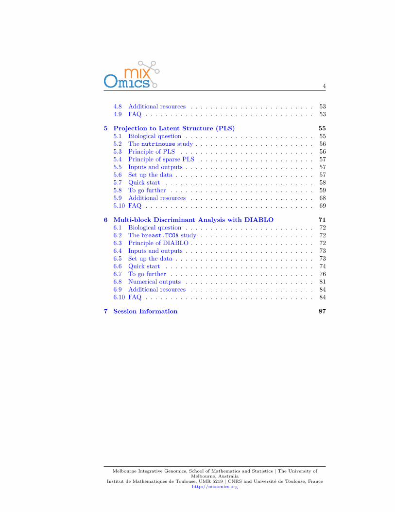
Our toolkit includes 17 new multivariate methodologies some depicted belowdepending on the data to integrate and the biological questions (e.g. exploration,discriminant analysis, data integration for 2 or more data sets).



https://github.com/mixOmicsTeam/Bookdown/issues

https://mixomics-users.discourse.group/

http://mixomics.org

6



http://mixomics.org

7

Chapter 1

Introduction

mixOmics is an R toolkit dedicated to the exploration and integration of bio-logical data sets with a specific focus on variable selection. The package cur-rently includes nineteen multivariate methodologies, mostly developed by themixOmics team (see some of our references in 1.2.3). Originally, all methodswere designed for omics data, however, their application is not limited to bi-ological data only. Other applications where integration is required can beconsidered, but mostly for the case where the predictor variables are continuous(see also 1.1).

In mixOmics, a strong focus is given to graphical representation to better trans-late and understand the relationships between the different data types and vi-sualize the correlation structure at both sample and variable levels.

1.1 Input dataNote the data pre-processing requirements before analysing data with mixOmics:

• Types of data. Different types of biological data can be explored andintegrated with mixOmics. Our methods can handle molecular featuresmeasured on a continuous scale (e.g. microarray, mass spectrometry-basedproteomics and metabolomics) or sequenced-based count data (RNA-seq,16S, shotgun metagenomics) that become ‘continuous’ data after pre-processing and normalisation.

• Normalisation. The package does not handle normalisation as it isplatform-specific and we cover a too wide variety of data! Prior to theanalysis, we assume the data sets have been normalised using appropriatenormalisation methods and pre-processed when applicable.

• Prefiltering. While mixOmics methods can handle large data sets (sev-eral tens of thousands of predictors), we recommend pre-filtering the data



http://mixomics.org

8

to less than 10K predictor variables per data set, for example by usingMedian Absolute Deviation (Teng et al., 2016) for RNA-seq data, by re-moving consistently low counts in microbiome data sets (Lê Cao et al.,2016) or by removing near-zero variance predictors. Such step aims tolessen the computational time during the parameter tuning process.

• Data format. Our methods use matrix decomposition techniques. There-fore, the numeric data matrix or data frames have n observations or sam-ples in rows and p predictors or variables (e.g. genes, proteins, OTUs) incolumns.

• Covariates. In the current version of mixOmics, covariates that mayconfound the analysis are not included in the methods. We recommendcorrecting for those covariates beforehand using appropriate univariate ormultivariate methods for batch effect removal. Contact us for more detailsas we are currently working on this aspect.

1.2 Methods1.2.1 Some background knowledgeWe list here the main methodological or theoretical concepts you need to knowto be able to efficiently apply mixOmics:

• Individuals, observations or samples: the experimental units onwhich information are collected, e.g. patients, cell lines, cells, faecal sam-ples etc.

• Variables, predictors: read-out measured on each sample, e.g. gene(expression), protein or OTU (abundance), weight etc.

• Variance: measures the spread of one variable. In our methods, weestimate the variance of components rather that variable read-outs. Ahigh variance indicates that the data points are very spread out from themean, and from one another (scattered).

• Covariance: measures the strength of the relationship between two vari-ables, i.e. whether they co-vary. A high covariance value indicates a strongrelationship, e.g. weight and height in individuals frequently vary roughlyin the same way; roughly, the heaviest are the tallest. A covariance valuehas no lower or upper bound.

• Correlation: a standardized version of the covariance that is boundedby -1 and 1.

• Linear combination: variables are combined by multiplying each ofthem by a coefficient and adding the results. A linear combination ofheight and weight could be 2 ∗ weight - 1.5 ∗ height with the coefficients2 and -1.5 assigned with weight and height respectively.



http://mixomics.org

9

• Component: an artificial variable built from a linear combination of theobserved variables in a given data set. Variable coefficients are optimallydefined based on some statistical criterion. For example in Principal Com-ponent Analysis, the coefficients of a (principal) component are defined soas to maximise the variance of the component.

• Loadings: variable coefficients used to define a component.

• Sample plot: representation of the samples projected in a small spacespanned (defined) by the components. Samples coordinates are deter-mined by their components values or scores.

• Correlation circle plot: representation of the variables in a spacespanned by the components. Each variable coordinate is defined as thecorrelation between the original variable value and each component. Acorrelation circle plot enables to visualise the correlation between variables- negative or positive correlation, defined by the cosine angle betweenthe centre of the circle and each variable point) and the contribution ofeach variable to each component - defined by the absolute value of thecoordinate on each component. For this interpretation, data need to becentred and scaled (by default in most of our methods except PCA). Formore details on this insightful graphic, see Figure 1 in (González et al.,2012).

• Unsupervised analysis: the method does not take into account anyknown sample groups and the analysis is exploratory. Examples of unsu-pervised methods covered in this vignette are Principal Component Anal-ysis (PCA, Chapter 3), Projection to Latent Structures (PLS, Chapter 5),and also Canonical Correlation Analysis (CCA, not covered here).

• Supervised analysis: the method includes a vector indicating the classmembership of each sample. The aim is to discriminate sample groupsand perform sample class prediction. Examples of supervised methodscovered in this vignette are PLS Discriminant Analysis (PLS-DA, Chapter4), DIABLO (Chapter 6) and also MINT (not covered here (Rohart et al.,2017b)).

1.2.2 Overview

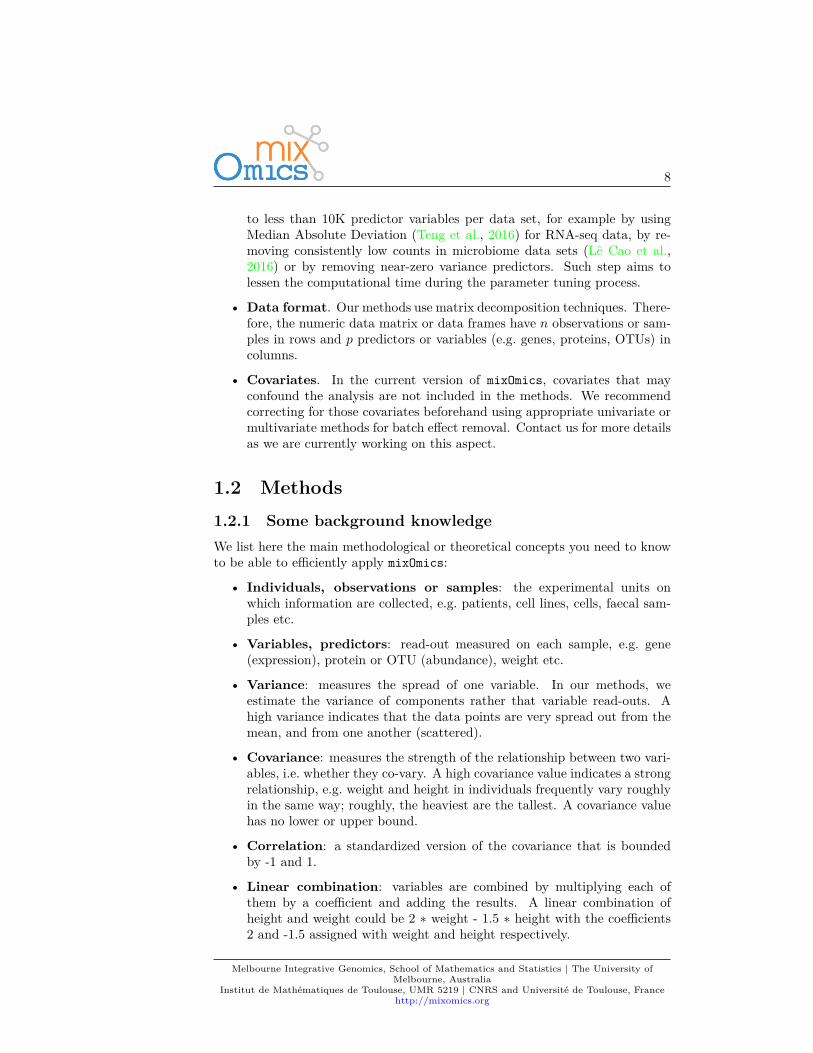
Here is an overview of the most widely used methods in mixOmics that will befurther detailed in this vignette, with the exception of rCCA and MINT. Wedepict them along with the type of data set they can handle.



http://mixomics.org

10

mixOmics overview

PCA

PLS−DA

PLS

DIABLO

Quantitative

Qualitative

1.2.3 Key publicationsThe methods implemented in mixOmics are described in detail in the followingpublications. A more extensive list can be found at this link.

• Overview and recent integrative methods: Rohart F., Gautier, B,Singh, A, Le Cao, K. A. mixOmics: an R package for ’omics feature selec-tion and multiple data integration. PLoS Comput Biol 13(11): e1005752.

• Graphical outputs for integrative methods: (González et al., 2012)Gonzalez I., Le Cao K.-A., Davis, M.D. and Dejean S. (2012) Insightfulgraphical outputs to explore relationships between two omics data sets.BioData Mining 5:19.

• DIABLO: Singh A, Gautier B, Shannon C, Vacher M, Rohart F, TebbuttS, K-A. Le Cao. DIABLO - multi-omics data integration for biomarkerdiscovery.

• sparse PLS: Le Cao K.-A., Martin P.G.P, Robert-Granie C. and Besse,P. (2009) Sparse Canonical Methods for Biological Data Integration: ap-plication to a cross-platform study. BMC Bioinformatics, 10:34.

• sparse PLS-DA: Le Cao K.-A., Boitard S. and Besse P. (2011) SparsePLS Discriminant Analysis: biologically relevant feature selection andgraphical displays for multiclass problems. BMC Bioinformatics, 22:253.



http://mixomics.org/a-propos/publications/

http://journals.plos.org/ploscompbiol/article?id=10.1371/journal.pcbi.1005752

http://journals.plos.org/ploscompbiol/article?id=10.1371/journal.pcbi.1005752

https://biodatamining.biomedcentral.com/articles/10.1186/1756-0381-5-19

https://biodatamining.biomedcentral.com/articles/10.1186/1756-0381-5-19

https://www.biorxiv.org/content/early/2018/03/20/067611

https://www.biorxiv.org/content/early/2018/03/20/067611

http://www.biomedcentral.com/1471-2105/10/34/

http://www.biomedcentral.com/1471-2105/10/34/

https://bmcbioinformatics.biomedcentral.com/articles/10.1186/1471-2105-12-253



http://mixomics.org

11

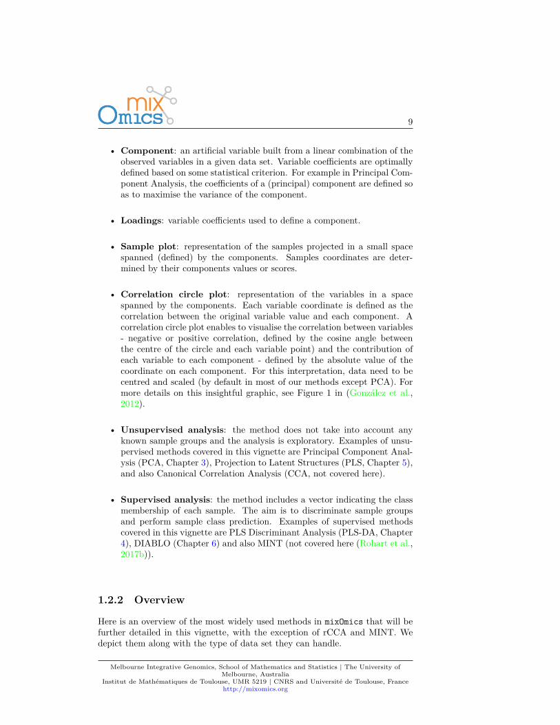
Figure 1.1: List of methods in mixOmics, sparse indicates methods that performvariable selection

• Multilevel approach for repeated measurements: Liquet B, Le CaoK-A, Hocini H, Thiebaut R (2012). A novel approach for biomarker se-lection and the integration of repeated measures experiments from twoassays. BMC Bioinformatics, 13:325

• sPLS-DA for microbiome data: Le Cao K-A∗, Costello ME ∗, LakisVA , Bartolo F, Chua XY, Brazeilles R and Rondeau P. (2016) MixMC:Multivariate insights into Microbial Communities.PLoS ONE 11(8):e0160169

1.3 Outline of this Vignette• Chapter 2 details some practical aspects to get started• Chapter 3: Principal Components Analysis (PCA)• Chapter 4: Projection to Latent Structure - Discriminant Analysis (PLS-

DA)• Chapter 5: Projection to Latent Structures (PLS)• Chapter 6: Integrative analysis for multiple data sets (DIABLO)






http://journals.plos.org/plosone/article?id=10.1371/journal.pone.0160169

http://journals.plos.org/plosone/article?id=10.1371/journal.pone.0160169

http://mixomics.org

12

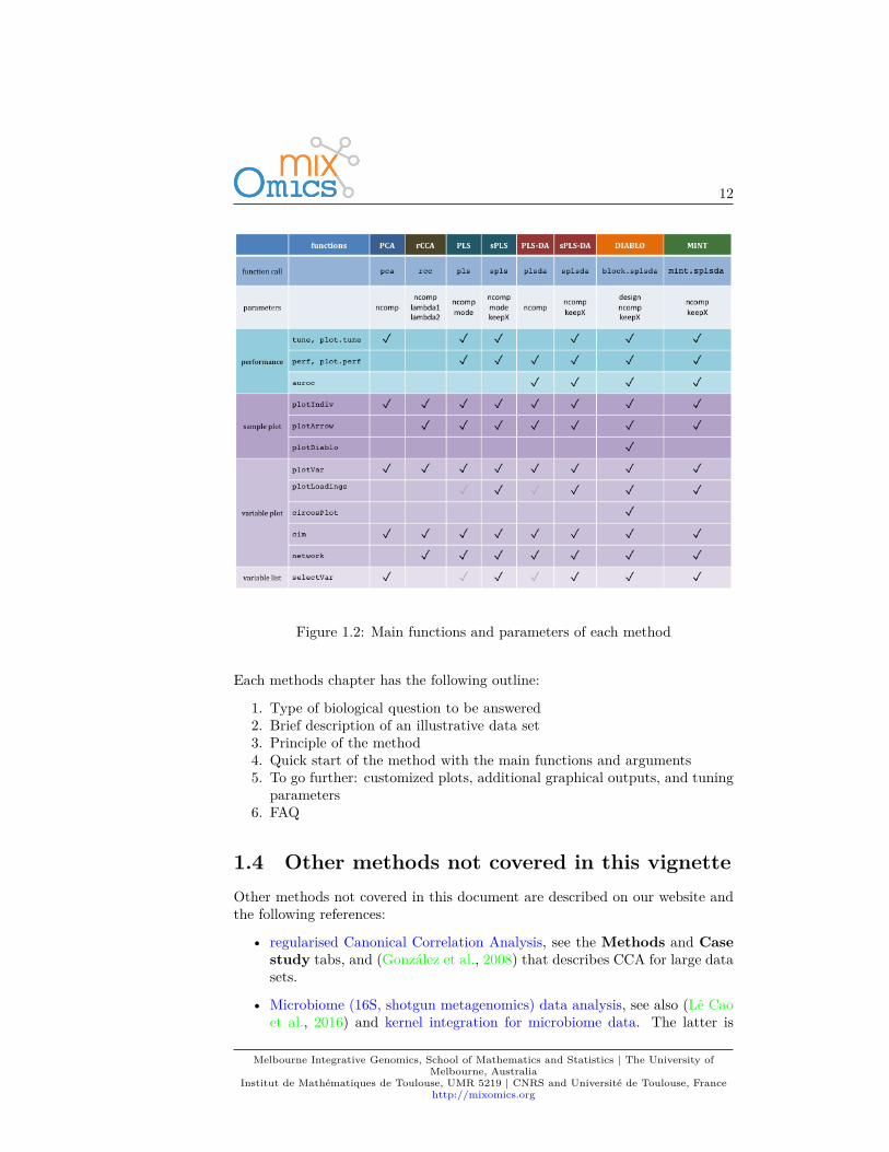
Figure 1.2: Main functions and parameters of each method

Each methods chapter has the following outline:

1. Type of biological question to be answered2. Brief description of an illustrative data set3. Principle of the method4. Quick start of the method with the main functions and arguments5. To go further: customized plots, additional graphical outputs, and tuning

parameters6. FAQ

1.4 Other methods not covered in this vignetteOther methods not covered in this document are described on our website andthe following references:

• regularised Canonical Correlation Analysis, see the Methods and Casestudy tabs, and (González et al., 2008) that describes CCA for large datasets.

• Microbiome (16S, shotgun metagenomics) data analysis, see also (Lê Caoet al., 2016) and kernel integration for microbiome data. The latter is



http://www.mixOmics.org

http://www.mixOmics.org/mixmc

http://mixomics.org/mixkernel

http://mixomics.org

13

in collaboration with Drs J Mariette and Nathalie Villa-Vialaneix (INRAToulouse, France), an example is provided for the Tara ocean metage-nomics and environmental data, see also (Mariette and Villa-Vialaneix,2017).

• MINT or P-integration to integrate independently generated transcrip-tomics data sets. An example in stem cells studies, see also (Rohart et al.,2017b).



http://mixomics.org/mixmint/

http://mixomics.org

14



http://mixomics.org

15

Chapter 2

Let’s get started

2.1 InstallationFirst, download the latest mixOmics version from Bioconductor:if (!requireNamespace("BiocManager", quietly = TRUE))

install.packages("BiocManager")BiocManager::install("mixOmics")

Alternatively, you can install the latest GitHub version of the package:BiocManager::install("mixOmicsTeam/mixOmics")

The mixOmics package should directly import the following packages:igraph, rgl, ellipse, corpcor, RColorBrewer, plyr, parallel,dplyr, tidyr, reshape2, methods, matrixStats, rARPACK, gridExtra.For Apple mac users: if you are unable to install the imported package rgl,you will need to install the XQuartz software first.

2.2 Load the packagelibrary(mixOmics)

Check that there is no error when loading the package, especially for the rgllibrary (see above).

2.3 Upload dataThe examples we give in this vignette use data that are already part of thepackage. To upload your own data, check first that your working directory is



https://www.xquartz.org

http://mixomics.org

16

set, then read your data from a .txt or .csv format, either by using File >Import Dataset in RStudio or via one of these command lines:# from csv filedata <- read.csv("your_data.csv", row.names = 1, header = TRUE)

# from txt filedata <- read.table("your_data.txt", header = TRUE)

For more details about the arguments used to modify those functions, type?read.csv or ?read.table in the R console.

2.4 Quick start in mixOmics

Each analysis should follow this workflow:

1. Run the method2. Graphical representation of the samples3. Graphical representation of the variables

Then use your critical thinking and additional functions and visual tools to makesense of your data! (some of which are listed in 1.2.2) and will be described inthe next Chapters.

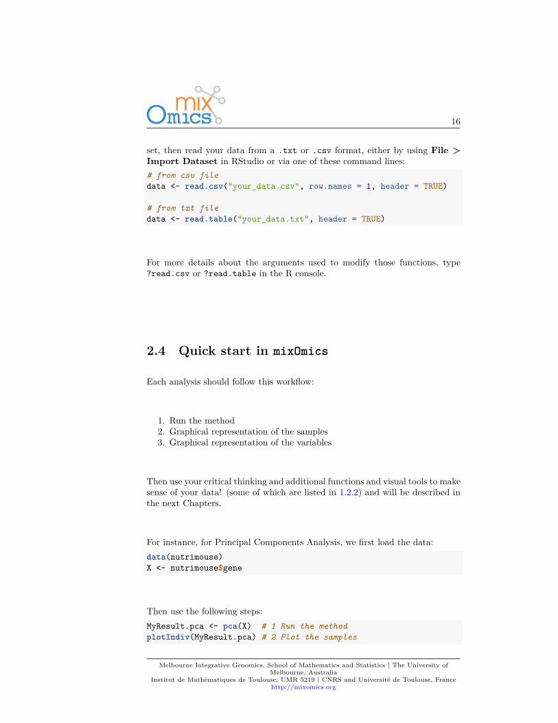
For instance, for Principal Components Analysis, we first load the data:data(nutrimouse)X <- nutrimouse$gene

Then use the following steps:MyResult.pca <- pca(X) # 1 Run the methodplotIndiv(MyResult.pca) # 2 Plot the samples



http://mixomics.org

17

1

2

3

4

5

6

7

8

9

10

11

12

13

14

15

16

17

18

19

20

21

22

23

24

25

26

2728

29

30

31

32

33

3435

36

37

38

39

40

PlotIndiv

−1 0 1

−1.0

−0.5

0.0

0.5

PC1: 35% expl. var

PC

2: 2

0% e

xpl.

var

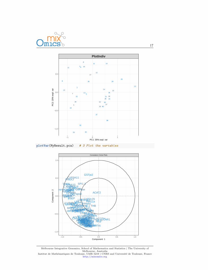
plotVar(MyResult.pca) # 3 Plot the variables

X36b4

ACAT1

ACAT2

ACBP

ACC1ACC2 ACOTH

ADISPADSS1

ALDH3

AM2R

AOX

BACT

BIENBSEP

Bcl.3

C16SR

CACP

CAR1

CBS

CIDEA

COX1COX2

CPT2

CYP24

CYP26

CYP27a1

CYP27b1CYP2b10CYP2b13

CYP2c29

CYP3A11

CYP4A10CYP4A14

CYP7a

CYP8b1

FAS

FAT

FDFT

FXRG6PDH

G6Pase

GK

GS

GSTaGSTmu

GSTpi2

HMGCoAred

HPNCL

IL.2

L.FABP

LCE

LDLr

LPK

LPLLXRaLXRb

LpinLpin1

Lpin2

Lpin3

M.CPT1MCAD

MDR1

MDR2MRP6

MS

MTHFR

NGFiBNURR1 NtcpOCTN2PAL

PDK4

PECI

PLTP

PMDCI

PON

PPARa

PPARd

PPARgPXR

Pex11a

RARaRARb2

RXRaRXRb2

RXRg1

S14

SHP1

SIAT4c

SPI1.1

SR.BI

THB

THIOL

TRaTRb

Tpalpha

Tpbeta

UCP2UCP3VDR

VLDLrWaf1ap2

apoA.I

apoBapoC3

apoE

c.fos

cHMGCoAScMOAT

eif2g

hABC1

i.BABP

i.BATi.FABP

i.NOS

mABC1

mHMGCoAS

Correlation Circle Plots

−1.0 −0.5 0.0 0.5 1.0

−1.0

−0.5

0.0

0.5

1.0

Component 1

Com

pone

nt 2



http://mixomics.org

18

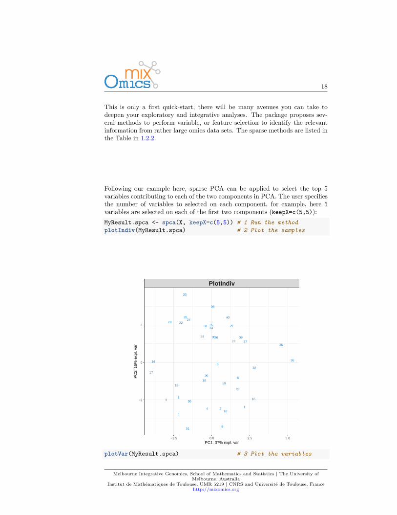
This is only a first quick-start, there will be many avenues you can take todeepen your exploratory and integrative analyses. The package proposes sev-eral methods to perform variable, or feature selection to identify the relevantinformation from rather large omics data sets. The sparse methods are listed inthe Table in 1.2.2.

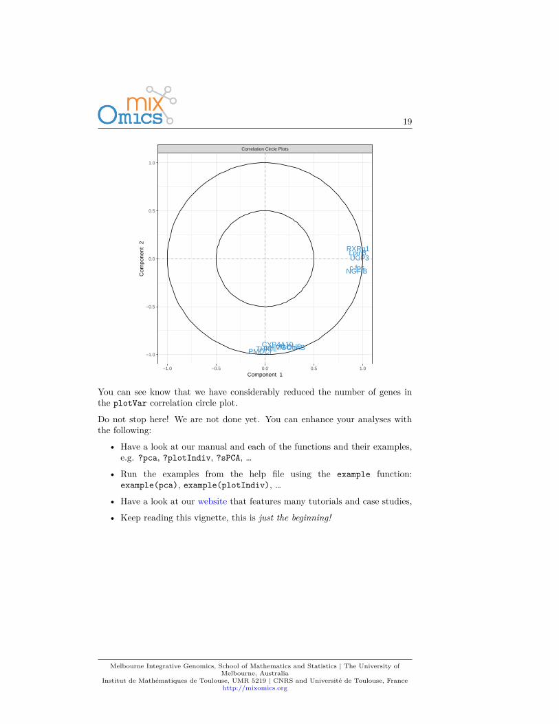
Following our example here, sparse PCA can be applied to select the top 5variables contributing to each of the two components in PCA. The user specifiesthe number of variables to selected on each component, for example, here 5variables are selected on each of the first two components (keepX=c(5,5)):MyResult.spca <- spca(X, keepX=c(5,5)) # 1 Run the methodplotIndiv(MyResult.spca) # 2 Plot the samples

1

2

3

4

5

6

7

8

9

10

11

12

13

14

1516

17

18

19

20

21

22

23

2425

26

27

28

29

30

31

32

33

3435

3637

38

39

40

PlotIndiv

−2.5 0.0 2.5 5.0

−2

0

2

PC1: 37% expl. var

PC

2: 1

6% e

xpl.

var

plotVar(MyResult.spca) # 3 Plot the variables



http://mixomics.org

19

ALDH3CYP4A10

Lpin3

NGFiB

PMDCI

RXRg1

THIOL

UCP3c.fos

mHMGCoAS


−1.0 −0.5 0.0 0.5 1.0

−1.0

−0.5

0.0

0.5

1.0

Component 1

Com

pone

nt 2

You can see know that we have considerably reduced the number of genes inthe plotVar correlation circle plot.

Do not stop here! We are not done yet. You can enhance your analyses withthe following:

• Have a look at our manual and each of the functions and their examples,e.g. ?pca, ?plotIndiv, ?sPCA, …

• Run the examples from the help file using the example function:example(pca), example(plotIndiv), …

• Have a look at our website that features many tutorials and case studies,

• Keep reading this vignette, this is just the beginning!



http://www.mixomics.org

http://mixomics.org

20



http://mixomics.org

21

Chapter 3

Principal ComponentAnalysis (PCA)

PCA overview

PCA

Quantitative

3.1 Biological questionI would like to identify the major sources of variation in my data and identify



http://mixomics.org

22

whether such sources of variation correspond to biological conditions or experi-mental bias. I would like to visualise trends or patterns between samples, whetherthey ‘naturally’ cluster according to known biological conditions.

3.2 The liver.toxicity studyThe liver.toxicity is a list in the package that contains:

• gene: a data frame with 64 rows and 3116 columns, corresponding to theexpression levels of 3,116 genes measured on 64 rats.

• clinic: a data frame with 64 rows and 10 columns, corresponding to themeasurements of 10 clinical variables on the same 64 rats.

• treatment: data frame with 64 rows and 4 columns, indicating the treat-ment information of the 64 rats, such as doses of acetaminophen and timesof necropsy.

• gene.ID: a data frame with 3116 rows and 2 columns, indicating geneBankIDs of the annotated genes.

More details are available at ?liver.toxicity.

To illustrate PCA, we focus on the expression levels of the genes in the dataframe liver.toxicity$gene. Some of the terms mentioned below are listed in1.2.1.

3.3 Principle of PCAThe aim of PCA (Jolliffe, 2005) is to reduce the dimensionality of the datawhilst retaining as much information as possible. ‘Information’ is referred hereas variance. The idea is to create uncorrelated artificial variables called prin-cipal components (PCs) that combine in a linear manner the original (possiblycorrelated) variables (e.g. genes, metabolites, etc.).

Dimension reduction is achieved by projecting the data into space spanned bythe principal components (PC). In practice, it means that each sample is as-signed a score on each new PC dimension - this score is calculated as a linearcombination of the original variables to which a weight is applied. The weightsof each of the original variables are stored in the so-called loading vectors as-sociated to each PC. The dimension of the data is reduced by projecting thedata into the smaller subspace spanned by the PCs, while capturing the largestsources of variation between samples.

The principal components are obtained so that their variance is maximised. Tothat end, we calculate the eigenvectors/eigenvalues of the variance-covariancematrix, often via singular value decomposition when the number of variablesis very large. The data are usually centred (center = TRUE), and sometimes



http://mixomics.org

23

scaled (scale = TRUE) in the method. The latter is especially advised in thecase where the variance is not homogeneous across variables.

The first PC is defined as the linear combination of the original variables thatexplains the greatest amount of variation. The second PC is then defined asthe linear combination of the original variables that accounts for the greatestamount of the remaining variation subject of being orthogonal (uncorrelated) tothe first component. Subsequent components are defined likewise for the otherPCA dimensions. The user must, therefore, report how much information isexplained by the first PCs as these are used to graphically represent the PCAoutputs.

3.4 Load the data

We first load the data from the package. See 2.2 to upload your own data.library(mixOmics)data(liver.toxicity)X <- liver.toxicity$gene

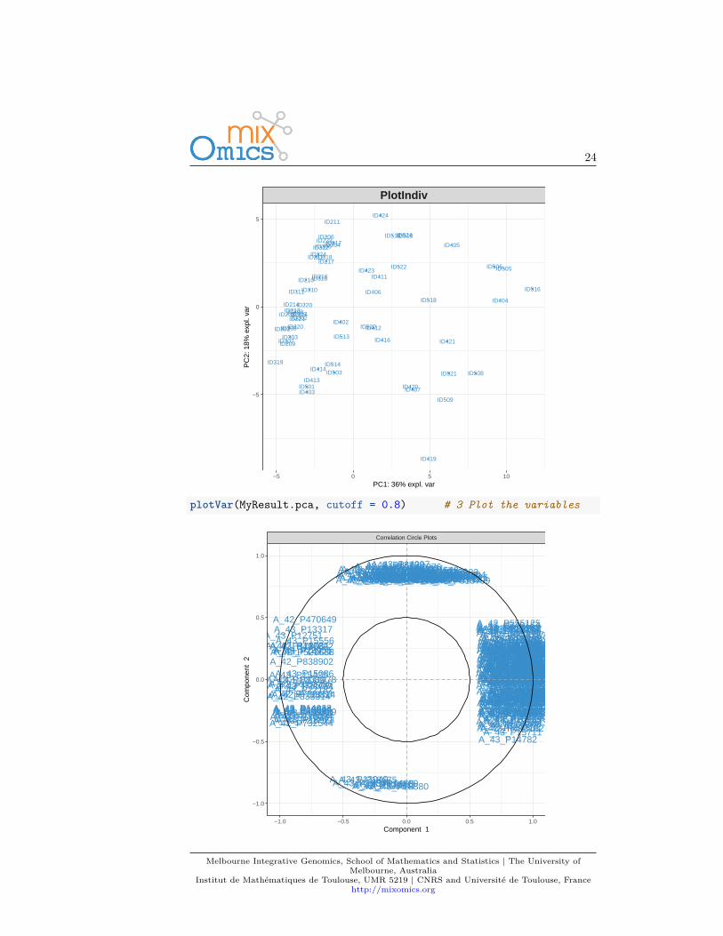
3.5 Quick startMyResult.pca <- pca(X) # 1 Run the methodplotIndiv(MyResult.pca) # 2 Plot the samples



http://mixomics.org

24

ID202

ID203

ID204ID206

ID208

ID209

ID210

ID211

ID212

ID213ID214

ID216

ID217

ID220

ID221

ID223

ID302

ID303

ID306

ID307

ID308

ID310ID311

ID312

ID314ID315

ID316

ID317

ID318

ID319

ID320

ID324

ID402

ID403

ID404

ID405

ID406

ID407

ID411

ID412

ID413

ID414

ID416

ID419

ID420

ID421

ID423

ID424

ID501

ID503

ID505ID506

ID508

ID509

ID510ID512

ID513

ID514

ID516

ID518

ID520

ID521

ID522

ID524

PlotIndiv

−5 0 5 10

−5

0

5

PC1: 36% expl. var

PC

2: 1

8% e

xpl.

var

plotVar(MyResult.pca, cutoff = 0.8) # 3 Plot the variables

A_43_P15845A_43_P13949A_42_P735647A_43_P19665A_43_P18675

A_43_P16094

A_42_P833314

A_43_P21799A_42_P599869

A_42_P732544

A_43_P19614A_43_P23389A_43_P12001A_43_P18923A_43_P17003

A_43_P16605A_43_P13450

A_43_P18880A_43_P12221A_43_P14809

A_42_P752916A_42_P750511A_43_P14997

A_42_P811256A_43_P12191A_43_P17772A_43_P18730

A_43_P15575A_43_P10147A_43_P11448A_43_P14197A_42_P526030

A_43_P15482

A_42_P470649

A_43_P14921A_42_P496622A_43_P12751

A_43_P13317A_43_P15556A_43_P17808

A_42_P838902

A_43_P11724

A_43_P15425A_43_P10089A_42_P652296

A_43_P12697A_43_P14184A_42_P531619A_43_P13225A_43_P11969

A_43_P14863A_43_P13266

A_43_P15086

A_43_P22955

A_42_P831978

A_42_P733814A_43_P21051

A_43_P14033

A_43_P22182A_42_P478500A_42_P738153

A_42_P521638A_42_P730292A_42_P721743

A_42_P501972

A_42_P555125A_42_P828727

A_42_P673838A_43_P17696

A_42_P827677A_42_P504523

A_42_P825183A_42_P651963A_42_P504367

A_43_P12128A_42_P529904

A_42_P767698A_42_P654031

A_43_P12417

A_43_P21855A_43_P11807A_42_P632361A_42_P545006A_42_P665106A_42_P617710A_43_P10981

A_43_P11936A_42_P840861

A_42_P712329

A_42_P591374A_42_P453685A_42_P748004

A_43_P19267

A_42_P598733A_43_P19128

A_42_P472580

A_42_P468595

A_43_P10744

A_42_P739047

A_43_P11789A_42_P790848

A_42_P473940A_43_P10029

A_42_P666030A_43_P17427A_42_P839061A_43_P10469

A_43_P11965

A_42_P459902

A_42_P813969

A_42_P755665

A_42_P564665

A_43_P17539

A_42_P554845

A_42_P731951A_42_P512252A_42_P559346A_42_P749154

A_43_P10585

A_42_P565161A_42_P842057

A_43_P16953

A_43_P22062

A_42_P744416A_43_P18742A_42_P766275A_43_P16995

A_43_P18004

A_43_P17082

A_42_P718146A_42_P597659

A_43_P23016

A_42_P702678

A_42_P810613A_42_P811912A_43_P16079A_42_P492740

A_42_P799947A_42_P628013

A_42_P513599

A_42_P568751

A_42_P705413

A_43_P17429

A_42_P696769A_43_P14675

A_42_P785770

A_42_P630562A_42_P802628A_42_P681650A_42_P552441A_42_P739860

A_42_P636498A_42_P698740A_43_P14864

A_43_P10003A_43_P17196

A_42_P613889

A_42_P717602

A_42_P515405

A_43_P17245A_42_P822390

A_42_P551055

A_43_P12811

A_42_P820863A_42_P760741

A_43_P10606

A_43_P12806

A_42_P636616

A_43_P14324A_42_P677628A_42_P769476

A_43_P12397

A_43_P12400A_42_P684538

A_42_P820597

A_42_P543226

A_42_P632078

A_42_P612834

A_42_P755831A_43_P16550A_42_P470474

A_42_P681533A_43_P22616

A_42_P550264A_43_P11644

A_42_P825290

A_43_P20962

A_43_P22419

A_43_P10006

A_42_P728230A_42_P840953

A_42_P675890A_43_P23376

A_42_P809565A_42_P620915A_42_P758454

A_42_P486763

A_42_P738559

A_43_P12571

A_42_P467246

A_42_P804499A_42_P834104

A_42_P824640A_42_P692317

A_43_P15205

A_42_P510530A_42_P538337A_42_P484423

A_42_P660936A_42_P797420A_42_P529681

A_43_P13713A_42_P779836

A_43_P12117A_43_P14517A_43_P12620A_42_P564637

A_42_P703375

A_43_P12543A_42_P480108A_42_P814010

A_42_P649851A_43_P11996

A_42_P547560A_42_P593767

A_42_P479251A_43_P16523A_43_P10645

A_42_P764413

A_43_P11477

A_42_P830405A_43_P11754A_42_P812008

A_42_P458472

A_43_P22220

A_42_P704648

A_42_P720521

A_43_P10665A_42_P819060A_42_P634760

A_42_P690300

A_43_P16453

A_42_P512460

A_43_P14163

A_43_P14782A_43_P15711A_42_P493162

A_43_P11472A_42_P469551A_42_P567268A_43_P13297

A_43_P18646A_42_P470836

A_43_P21383

A_42_P654538

A_42_P607720A_43_P15258A_42_P734037

A_42_P471835A_42_P545943

A_43_P14566A_42_P731280

A_42_P673212A_42_P480915A_43_P12832A_42_P499383

A_42_P479328A_43_P16990A_43_P16590

A_42_P683328

A_42_P720081A_42_P655825

A_42_P506968

A_42_P785370

A_42_P706032A_42_P586270

A_42_P591460

A_42_P598934A_42_P654018

A_42_P655644A_42_P635611A_43_P13577A_42_P491221A_43_P12617A_43_P11865A_43_P10390A_42_P595403A_42_P701991A_43_P17276

A_43_P10854A_43_P11893A_42_P765427

A_42_P582747A_42_P556457A_42_P499075A_42_P770410A_43_P16327

A_43_P21648A_42_P721655A_43_P18437A_42_P601737A_42_P815235A_42_P686798A_43_P13183A_42_P648862A_42_P456713A_42_P517060A_42_P695704A_42_P544436A_43_P20260

A_43_P12712A_42_P549825A_42_P616370A_42_P813799A_42_P637583A_42_P696251A_42_P767737A_42_P686916A_42_P681634A_43_P18983A_42_P533091A_42_P581645A_43_P22567


−1.0 −0.5 0.0 0.5 1.0

−1.0

−0.5

0.0

0.5

1.0

Component 1

Com

pone

nt 2



http://mixomics.org

25

If you were to run pca with this minimal code, you would be using the followingdefault values:

• ncomp =2: the first two principal components are calculated and are usedfor graphical outputs;

• center = TRUE: data are centred (mean = 0)• scale = FALSE: data are not scaled. If scale = TRUE standardizes each

variable (variance = 1).

Other arguments can also be chosen, see ?pca.

This example was shown in Chapter 2.4. The two plots are not extremely mean-ingful as specific sample patterns should be further investigated and the variablecorrelation circle plot contains too many variables to be easily interpreted. Let’simprove those graphics as shown below to improve interpretation.

3.6 To go further

3.6.1 Customize plots

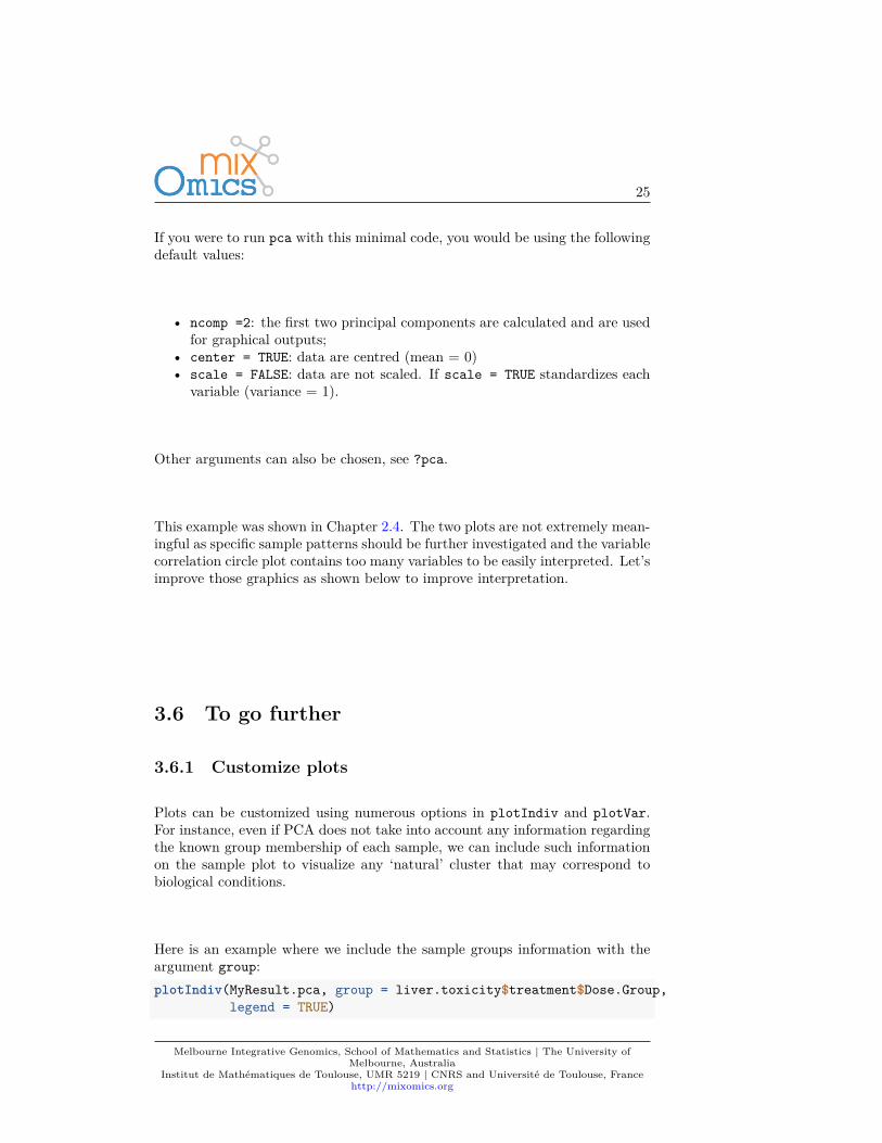
Plots can be customized using numerous options in plotIndiv and plotVar.For instance, even if PCA does not take into account any information regardingthe known group membership of each sample, we can include such informationon the sample plot to visualize any ‘natural’ cluster that may correspond tobiological conditions.

Here is an example where we include the sample groups information with theargument group:plotIndiv(MyResult.pca, group = liver.toxicity$treatment$Dose.Group,

legend = TRUE)



http://mixomics.org

26

ID202

ID203

ID204ID206

ID208

ID209

ID210

ID211

ID212

ID213ID214

ID216

ID217

ID220

ID221

ID223

ID302

ID303

ID306

ID307

ID308

ID310ID311

ID312

ID314ID315

ID316

ID317

ID318

ID319

ID320

ID324

ID402

ID403

ID404

ID405

ID406

ID407

ID411

ID412

ID413

ID414

ID416

ID419

ID420

ID421

ID423

ID424

ID501

ID503

ID505ID506

ID508

ID509

ID510ID512

ID513

ID514

ID516

ID518

ID520

ID521

ID522

ID524

PlotIndiv

−5 0 5 10

−5

0

5

PC1: 36% expl. var

PC

2: 1

8% e

xpl.

var

Legend

50

150

1500

2000

Additionally, two factors can be displayed using both colours (argument group)and symbols (argument pch). For example here we display both Dose and Timeof exposure and improve the title and legend:plotIndiv(MyResult.pca, ind.names = FALSE,

group = liver.toxicity$treatment$Dose.Group,pch = as.factor(liver.toxicity$treatment$Time.Group),legend = TRUE, title = 'Liver toxicity: genes, PCA comp 1 - 2',legend.title = 'Dose', legend.title.pch = 'Exposure')



http://mixomics.org

27

Liver toxicity: genes, PCA comp 1 − 2

−5 0 5 10

−5

0

5

PC1: 36% expl. var

PC

2: 1

8% e

xpl.

var

Dose

50

150

1500

2000

Exposure

18

24

48

6

By including information related to the dose of acetaminophen and time ofexposure enables us to see a cluster of low dose samples (blue and orange, topleft at 50 and 100mg respectively), whereas samples with high doses (1500 and2000mg in grey and green respectively) are more scattered, but highlight anexposure effect.

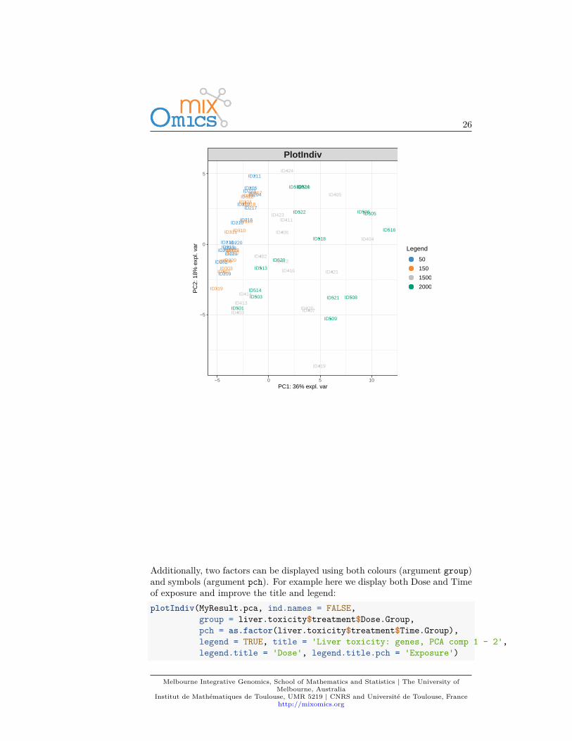
To display the results on other components, we can change the comp argumentprovided we have requested enough components to be calculated. Here is oursecond PCA with 3 components:MyResult.pca2 <- pca(X, ncomp = 3)plotIndiv(MyResult.pca2, comp = c(1,3), legend = TRUE,

group = liver.toxicity$treatment$Time.Group,title = 'Multidrug transporter, PCA comp 1 - 3')



http://mixomics.org

28

ID202ID203

ID213

ID214ID302ID303ID314ID315

ID402

ID403

ID413

ID414ID501

ID503

ID513ID514

ID204

ID206

ID216

ID217ID306ID316ID317ID318

ID404ID405

ID406

ID416

ID505

ID506

ID516

ID518

ID208

ID209

ID220ID221

ID307

ID308ID319

ID320ID407

ID419

ID420

ID421

ID508

ID509ID520

ID521

ID210

ID211

ID212ID223

ID310

ID311ID312ID324

ID411

ID412

ID423ID424

ID510

ID512

ID522

ID524

Multidrug transporter, PCA comp 1 − 3

−5 0 5 10

−5.0

−2.5

0.0

2.5

5.0

PC1: 36% expl. var

PC

3: 9

% e

xpl.

var Legend

6

18

24

48

Here, the 3rd component on the y-axis clearly highlights a time of exposureeffect.

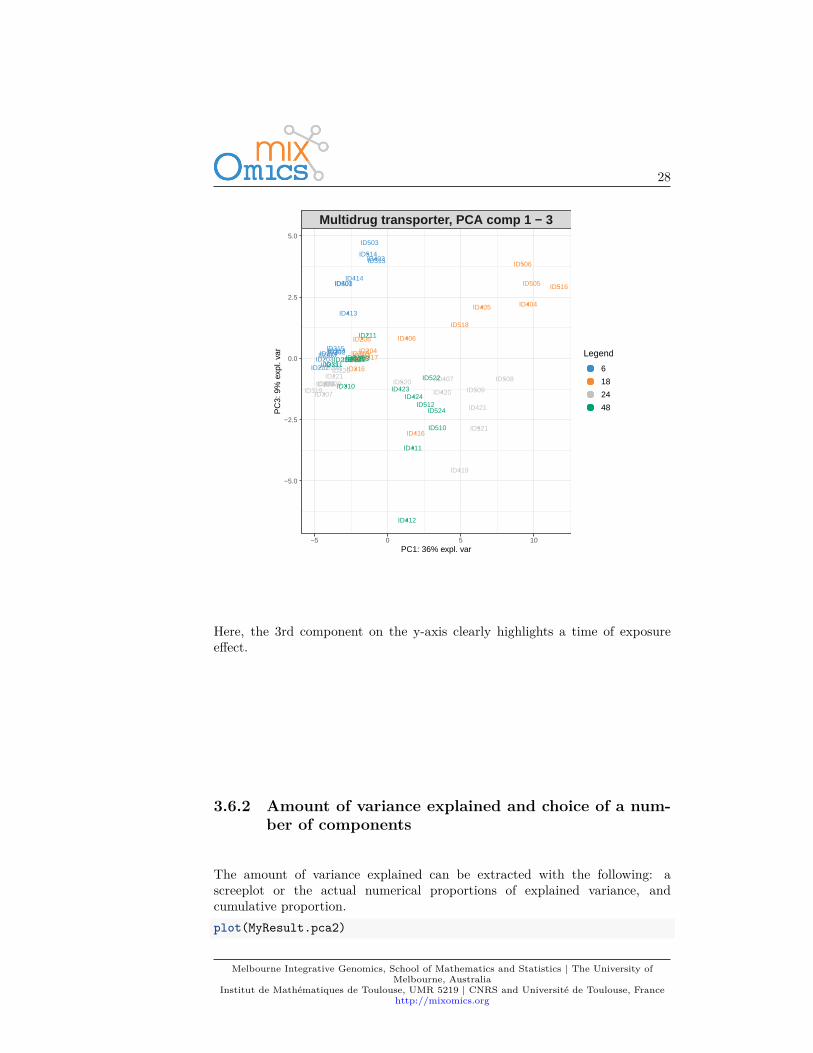
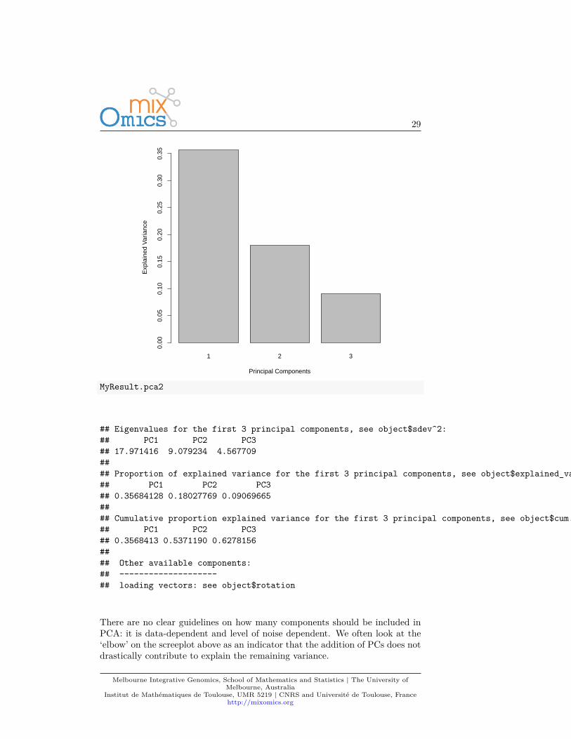
3.6.2 Amount of variance explained and choice of a num-ber of components

The amount of variance explained can be extracted with the following: ascreeplot or the actual numerical proportions of explained variance, andcumulative proportion.plot(MyResult.pca2)



http://mixomics.org

29

1 2 3

Principal Components

Exp

lain

ed V

aria

nce

0.00

0.05

0.10

0.15

0.20

0.25

0.30

0.35

MyResult.pca2

## Eigenvalues for the first 3 principal components, see object$sdev^2:## PC1 PC2 PC3## 17.971416 9.079234 4.567709#### Proportion of explained variance for the first 3 principal components, see object$explained_variance:## PC1 PC2 PC3## 0.35684128 0.18027769 0.09069665#### Cumulative proportion explained variance for the first 3 principal components, see object$cum.var:## PC1 PC2 PC3## 0.3568413 0.5371190 0.6278156#### Other available components:## --------------------## loading vectors: see object$rotation

There are no clear guidelines on how many components should be included inPCA: it is data-dependent and level of noise dependent. We often look at the‘elbow’ on the screeplot above as an indicator that the addition of PCs does notdrastically contribute to explain the remaining variance.



http://mixomics.org

30

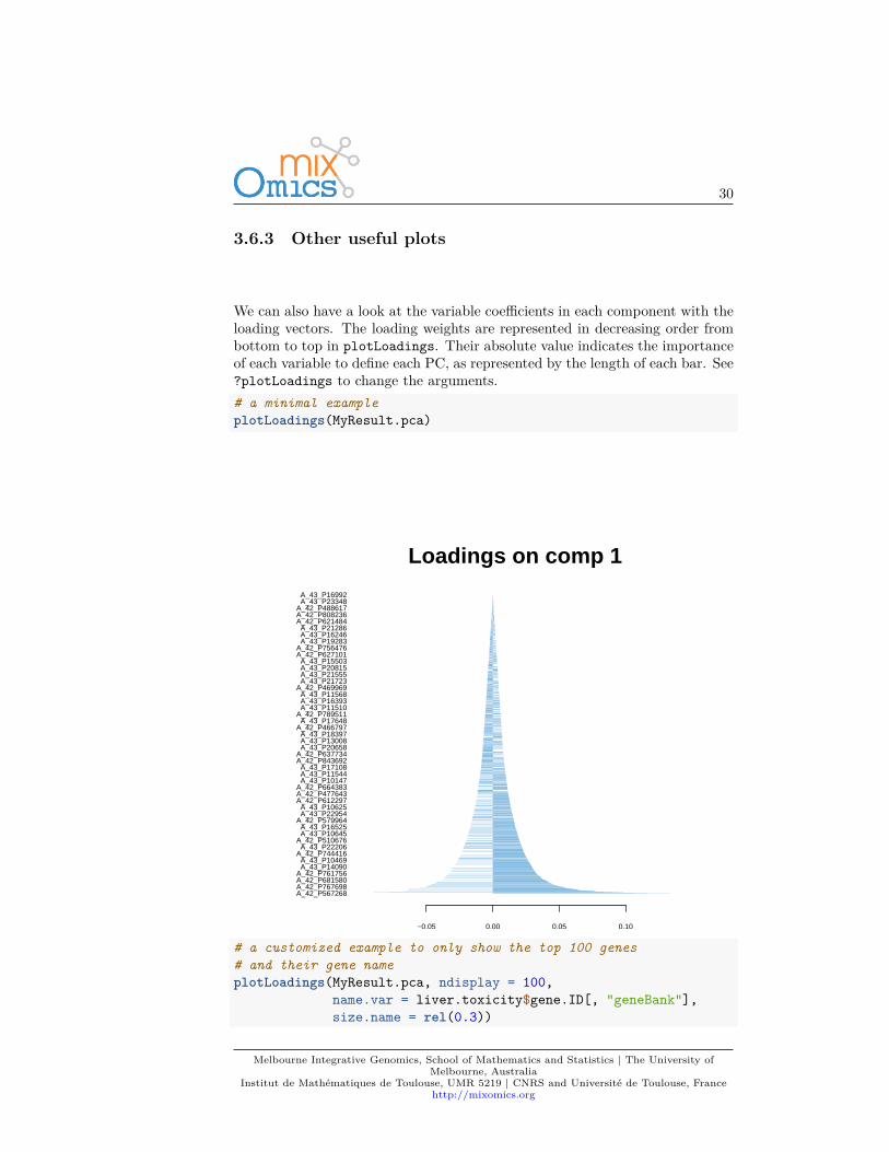
3.6.3 Other useful plots

We can also have a look at the variable coefficients in each component with theloading vectors. The loading weights are represented in decreasing order frombottom to top in plotLoadings. Their absolute value indicates the importanceof each variable to define each PC, as represented by the length of each bar. See?plotLoadings to change the arguments.# a minimal exampleplotLoadings(MyResult.pca)

A_42_P567268A_42_P767698A_42_P681580A_42_P761756

A_43_P14090A_43_P10469

A_42_P744416A_43_P22206

A_42_P510676A_43_P10645A_43_P16525

A_42_P579964A_43_P22954A_43_P10625

A_42_P612297A_42_P477643A_42_P664383

A_43_P10147A_43_P11544A_43_P17108

A_42_P843692A_42_P637734

A_43_P20658A_43_P13008A_43_P18397

A_42_P466797A_43_P17648

A_42_P789511A_43_P11510A_43_P16393A_43_P11568

A_42_P469969A_43_P21723A_43_P21555A_43_P20815A_43_P15503

A_42_P627101A_42_P756476

A_43_P19283A_43_P16246A_43_P21286

A_42_P621484A_42_P808236A_42_P488617

A_43_P23348A_43_P16992

−0.05 0.00 0.05 0.10

Loadings on comp 1

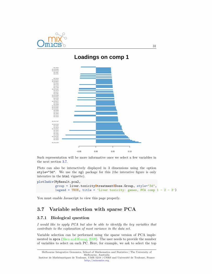
# a customized example to only show the top 100 genes# and their gene nameplotLoadings(MyResult.pca, ndisplay = 100,

name.var = liver.toxicity$gene.ID[, "geneBank"],size.name = rel(0.3))



http://mixomics.org

31

NM_001137564

NM_031642

NM_138826

NM_001011901

NM_013098

NM_024351

NM_024127

NM_153312

NM_001108441

NR_002704

NM_019291

XM_001079678

NM_001173437

NM_022229

NM_013120

NM_138504

NM_013134

NM_053968

NM_001003401

NM_001108487

NM_001109022

NM_031986

NM_053464

NM_001106147

XM_227081

NM_012495

NM_001034912

NM_001106689

NM_012801

NM_057211

NM_057133

NM_001109022

NM_177928

NM_019376

NM_017332

NM_053516

NM_001008337

NM_001004415

NM_031344

NM_012621

NM_138827

NM_001007634

NM_001004082

NM_053352

−0.05 0.00 0.05 0.10

Loadings on comp 1

Such representation will be more informative once we select a few variables inthe next section 3.7.

Plots can also be interactively displayed in 3 dimensions using the optionstyle="3d". We use the rgl package for this (the interative figure is onlyinteratice in the html vignette).plotIndiv(MyResult.pca2,

group = liver.toxicity$treatment$Dose.Group, style="3d",legend = TRUE, title = 'Liver toxicity: genes, PCA comp 1 - 2 - 3')

You must enable Javascript to view this page properly.

3.7 Variable selection with sparse PCA3.7.1 Biological questionI would like to apply PCA but also be able to identify the key variables thatcontribute to the explanation of most variance in the data set.

Variable selection can be performed using the sparse version of PCA imple-mented in spca (Shen and Huang, 2008). The user needs to provide the numberof variables to select on each PC. Here, for example, we ask to select the top



http://mixomics.org

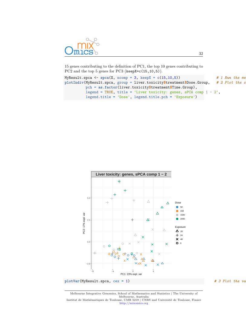
32

15 genes contributing to the definition of PC1, the top 10 genes contributing toPC2 and the top 5 genes for PC3 (keepX=c(15,10,5)).MyResult.spca <- spca(X, ncomp = 3, keepX = c(15,10,5)) # 1 Run the methodplotIndiv(MyResult.spca, group = liver.toxicity$treatment$Dose.Group, # 2 Plot the samples

pch = as.factor(liver.toxicity$treatment$Time.Group),legend = TRUE, title = 'Liver toxicity: genes, sPCA comp 1 - 2',legend.title = 'Dose', legend.title.pch = 'Exposure')

Liver toxicity: genes, sPCA comp 1 − 2

−8 −4 0 4

−2.5

0.0

2.5

5.0

PC1: 23% expl. var

PC

2: 1

7% e

xpl.

var

Dose

50

150

1500

2000

Exposure

18

24

48

6

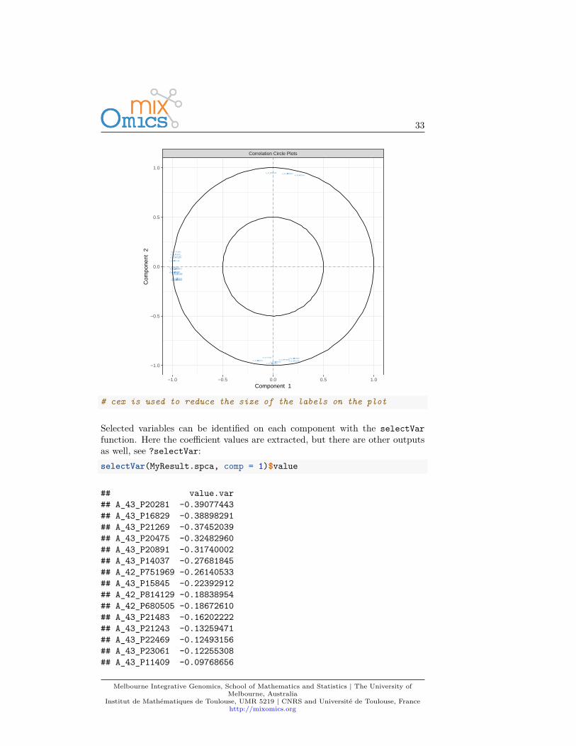
plotVar(MyResult.spca, cex = 1) # 3 Plot the variables



http://mixomics.org

33

A_43_P20891

A_43_P23061

A_43_P22469

A_43_P21243

A_43_P14037

A_43_P21269

A_43_P15845

A_43_P11409A_43_P16829

A_43_P20475

A_42_P680505

A_43_P20281A_42_P814129

A_43_P21483A_42_P751969

A_42_P620095

A_42_P761756A_42_P708480

A_42_P795796A_42_P470649

A_43_P12751

A_43_P13317

A_43_P22616A_42_P545943A_42_P765066


−1.0 −0.5 0.0 0.5 1.0

−1.0

−0.5

0.0

0.5

1.0

Component 1

Com

pone

nt 2

# cex is used to reduce the size of the labels on the plot

Selected variables can be identified on each component with the selectVarfunction. Here the coefficient values are extracted, but there are other outputsas well, see ?selectVar:selectVar(MyResult.spca, comp = 1)$value

## value.var## A_43_P20281 -0.39077443## A_43_P16829 -0.38898291## A_43_P21269 -0.37452039## A_43_P20475 -0.32482960## A_43_P20891 -0.31740002## A_43_P14037 -0.27681845## A_42_P751969 -0.26140533## A_43_P15845 -0.22392912## A_42_P814129 -0.18838954## A_42_P680505 -0.18672610## A_43_P21483 -0.16202222## A_43_P21243 -0.13259471## A_43_P22469 -0.12493156## A_43_P23061 -0.12255308## A_43_P11409 -0.09768656



http://mixomics.org

34

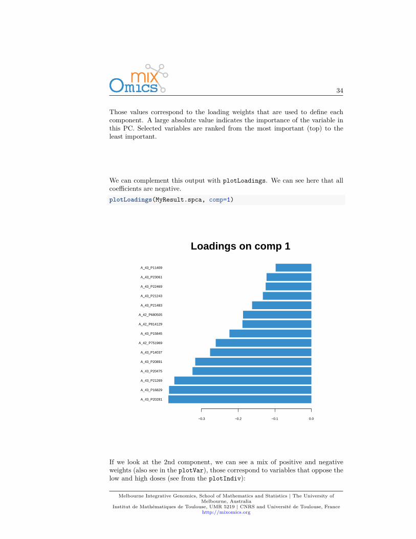
Those values correspond to the loading weights that are used to define eachcomponent. A large absolute value indicates the importance of the variable inthis PC. Selected variables are ranked from the most important (top) to theleast important.

We can complement this output with plotLoadings. We can see here that allcoefficients are negative.plotLoadings(MyResult.spca, comp=1)

A_43_P20281

A_43_P16829

A_43_P21269

A_43_P20475

A_43_P20891

A_43_P14037

A_42_P751969

A_43_P15845

A_42_P814129

A_42_P680505

A_43_P21483

A_43_P21243

A_43_P22469

A_43_P23061

A_43_P11409

−0.3 −0.2 −0.1 0.0

Loadings on comp 1

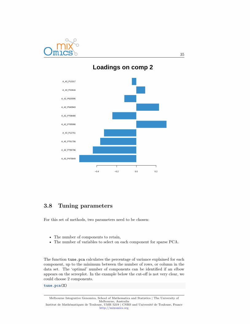
If we look at the 2nd component, we can see a mix of positive and negativeweights (also see in the plotVar), those correspond to variables that oppose thelow and high doses (see from the plotIndiv):



http://mixomics.org

35

A_42_P470649

A_42_P795796

A_42_P761756

A_43_P12751

A_42_P765066

A_42_P708480

A_42_P545943

A_42_P620095

A_43_P22616

A_43_P13317

−0.4 −0.2 0.0 0.2

Loadings on comp 2

3.8 Tuning parameters

For this set of methods, two parameters need to be chosen:

• The number of components to retain,• The number of variables to select on each component for sparse PCA.

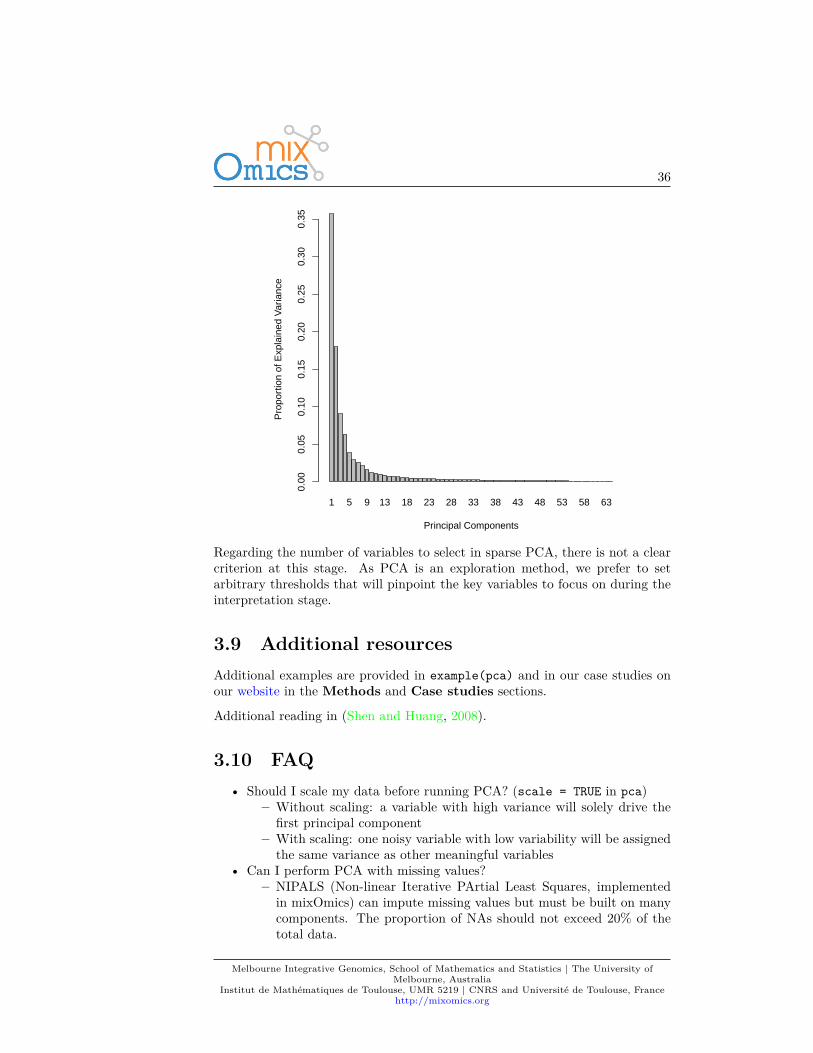
The function tune.pca calculates the percentage of variance explained for eachcomponent, up to the minimum between the number of rows, or column in thedata set. The ‘optimal’ number of components can be identified if an elbowappears on the screeplot. In the example below the cut-off is not very clear, wecould choose 2 components.tune.pca(X)



http://mixomics.org

36

1 5 9 13 18 23 28 33 38 43 48 53 58 63

Principal Components

Pro

port

ion

of E

xpla

ined

Var

ianc

e

0.00

0.05

0.10

0.15

0.20

0.25

0.30

0.35

Regarding the number of variables to select in sparse PCA, there is not a clearcriterion at this stage. As PCA is an exploration method, we prefer to setarbitrary thresholds that will pinpoint the key variables to focus on during theinterpretation stage.

3.9 Additional resourcesAdditional examples are provided in example(pca) and in our case studies onour website in the Methods and Case studies sections.

Additional reading in (Shen and Huang, 2008).

3.10 FAQ• Should I scale my data before running PCA? (scale = TRUE in pca)

– Without scaling: a variable with high variance will solely drive thefirst principal component

– With scaling: one noisy variable with low variability will be assignedthe same variance as other meaningful variables

• Can I perform PCA with missing values?– NIPALS (Non-linear Iterative PArtial Least Squares, implemented

in mixOmics) can impute missing values but must be built on manycomponents. The proportion of NAs should not exceed 20% of thetotal data.




http://mixomics.org

37

• When should I apply a multilevel approach in PCA? (multilevel argu-ment in PCA)

– When the unique individuals are measured more than once (repeatedmeasures)

– When the individual variation is less than treatment or time varia-tion. This means that samples from each unique individual will tendto cluster rather than the treatments.

– When a multilevel vs no multilevel seems to visually make a differenceon a PCA plot

– More details in this case study• When should I apply a CLR transformation in PCA? (logratio = 'CLR'

argument in PCA)– When data are compositional, i.e. expressed as relative proportions.

This is usually the case with microbiome studies as a result of pre-processing and normalisation, see more details here and in our casestudies in the same tab.



http://mixomics.org/case-studies/multilevel-vac18/

http://mixomics.org/mixmc/

http://mixomics.org

38



http://mixomics.org

39

Chapter 4

PLS - DiscriminantAnalysis (PLS-DA)

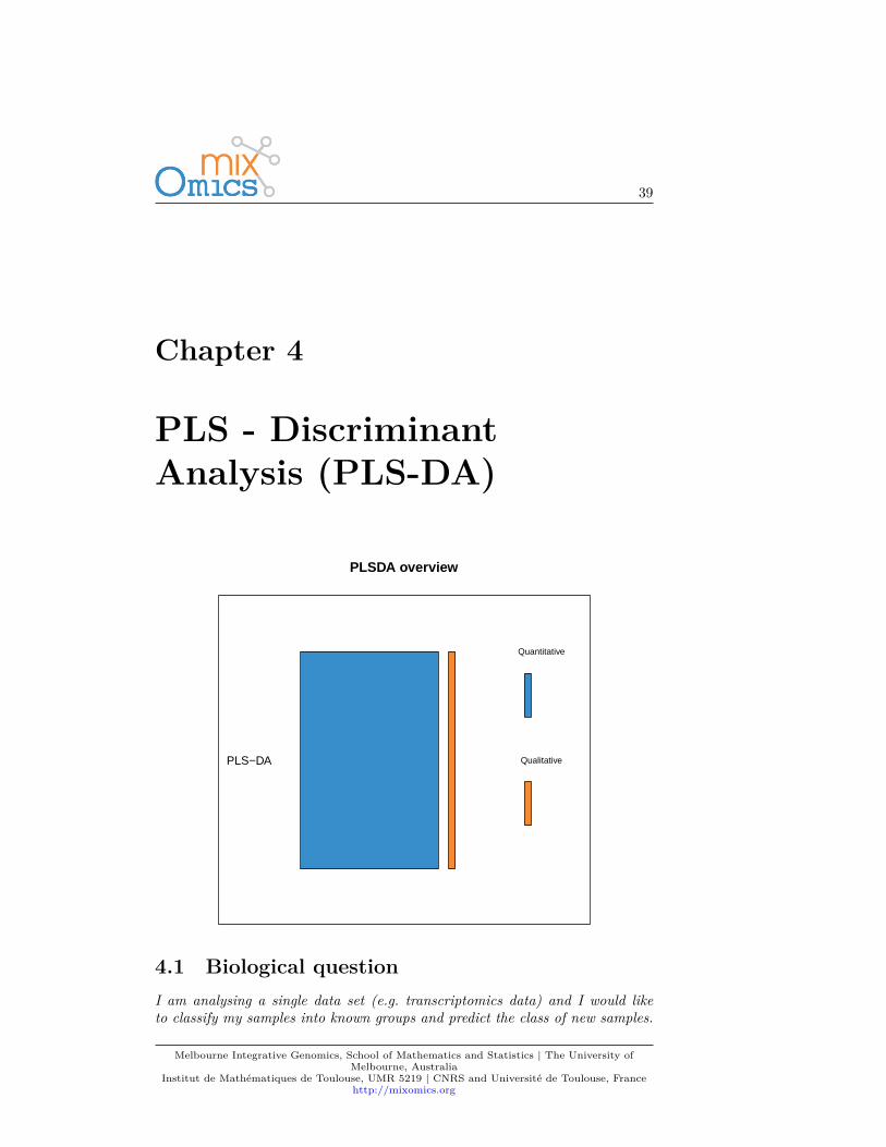
PLSDA overview

PLS−DA

Quantitative

Qualitative

4.1 Biological questionI am analysing a single data set (e.g. transcriptomics data) and I would liketo classify my samples into known groups and predict the class of new samples.



http://mixomics.org

40

In addition, I am interested in identifying the key variables that drive suchdiscrimination.

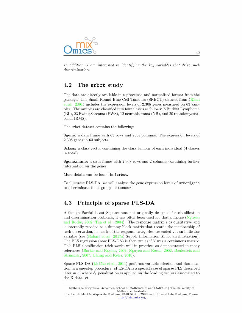
4.2 The srbct studyThe data are directly available in a processed and normalised format from thepackage. The Small Round Blue Cell Tumours (SRBCT) dataset from (Khanet al., 2001) includes the expression levels of 2,308 genes measured on 63 sam-ples. The samples are classified into four classes as follows: 8 Burkitt Lymphoma(BL), 23 Ewing Sarcoma (EWS), 12 neuroblastoma (NB), and 20 rhabdomyosar-coma (RMS).

The srbct dataset contains the following:

$gene: a data frame with 63 rows and 2308 columns. The expression levels of2,308 genes in 63 subjects.

$class: a class vector containing the class tumour of each individual (4 classesin total).

$gene.name: a data frame with 2,308 rows and 2 columns containing furtherinformation on the genes.

More details can be found in ?srbct.

To illustrate PLS-DA, we will analyse the gene expression levels of srbct$geneto discriminate the 4 groups of tumours.

4.3 Principle of sparse PLS-DAAlthough Partial Least Squares was not originally designed for classificationand discrimination problems, it has often been used for that purpose (Nguyenand Rocke, 2002; Tan et al., 2004). The response matrix Y is qualitative andis internally recoded as a dummy block matrix that records the membership ofeach observation, i.e. each of the response categories are coded via an indicatorvariable (see (Rohart et al., 2017a) Suppl. Information S1 for an illustration).The PLS regression (now PLS-DA) is then run as if Y was a continuous matrix.This PLS classification trick works well in practice, as demonstrated in manyreferences (Barker and Rayens, 2003; Nguyen and Rocke, 2002; Boulesteix andStrimmer, 2007; Chung and Keles, 2010).

Sparse PLS-DA (Lê Cao et al., 2011) performs variable selection and classifica-tion in a one-step procedure. sPLS-DA is a special case of sparse PLS describedlater in 5, where ℓ1 penalization is applied on the loading vectors associated tothe X data set.



http://mixomics.org

41

4.4 Inputs and outputsWe use the following data input matrices: X is a n × p data matrix, Y is afactor vector of length n that indicates the class of each sample, and Y ∗ is theassociated dummy matrix (n × K) with n the number of samples (individuals),p the number of variables and K the number of classes. PLS-DA main outputsare:

• A set of components, also called latent variables. There are as manycomponents as the chosen dimension of the PLS-DA model.

• A set of loading vectors, which are coefficients assigned to each vari-able to define each component. These coefficients indicate the importanceof each variable in PLS-DA. Importantly, each loading vector is associ-ated to a particular component. Loading vectors are obtained so thatthe covariance between a linear combination of the variables from X (theX-component) and the factor of interest Y (the Y ∗-component) is max-imised.

• A list of selected variables from X and associated to each componentif sPLS-DA is applied.

4.5 Set up the dataWe first load the data from the package. See 2.2 to upload your own data.

We will mainly focus on sparse PLS-DA that is more suited for large biologicaldata sets where the aim is to identify molecular signatures, as well as classifyingsamples. We first set up the data as X expression matrix and Y as a factor indi-cating the class membership of each sample. We also check that the dimensionsare correct and match:library(mixOmics)data(srbct)X <- srbct$geneY <- srbct$classsummary(Y) ## class summary

## EWS BL NB RMS## 23 8 12 20dim(X) ## number of samples and features

## [1] 63 2308length(Y) ## length of class memebrship factor = number of samples

## [1] 63



http://mixomics.org

42

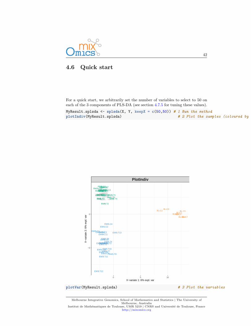
4.6 Quick start

For a quick start, we arbitrarily set the number of variables to select to 50 oneach of the 3 components of PLS-DA (see section 4.7.5 for tuning these values).MyResult.splsda <- splsda(X, Y, keepX = c(50,50)) # 1 Run the methodplotIndiv(MyResult.splsda) # 2 Plot the samples (coloured by classes automatically)

EWS.T1EWS.T2EWS.T3EWS.T4

EWS.T6

EWS.T7EWS.T9

EWS.T11

EWS.T12

EWS.T13

EWS.T14EWS.T15

EWS.T19

EWS.C8

EWS.C3

EWS.C2EWS.C4

EWS.C6

EWS.C9EWS.C7

EWS.C1

EWS.C11EWS.C10

BL.C5BL.C6

BL.C7

BL.C8BL.C1

BL.C2

BL.C3BL.C4

NB.C1NB.C2

NB.C3NB.C6NB.C12

NB.C7

NB.C4NB.C5

NB.C10NB.C11NB.C9

NB.C8

RMS.C4

RMS.C3

RMS.C9RMS.C2

RMS.C5RMS.C6

RMS.C7RMS.C8

RMS.C10RMS.C11

RMS.T1

RMS.T4

RMS.T2

RMS.T6

RMS.T7

RMS.T8RMS.T5

RMS.T3

RMS.T10

RMS.T11

PlotIndiv

0 5 10

−5

0

X−variate 1: 6% expl. var

X−

varia

te 2

: 6%

exp

l. va

r

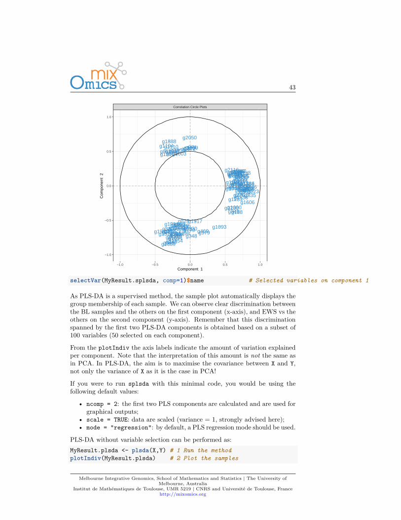
plotVar(MyResult.splsda) # 3 Plot the variables



http://mixomics.org

43

g29g36 g52

g74

g85 g123g165g166

g187

g188

g190

g229

g246

g276g335

g336g348g368

g373 g469

g509

g545

g555

g566

g585g589

g758

g779

g780g783

g803g820

g828

g836g846

g849

g867g971

g979

g998

g1003

g1008

g1036g1042

g1049

g1067

g1074

g1089

g1090

g1093

g1099

g1110

g1116

g1158

g1194

g1206

g1207

g1279

g1283

g1295

g1298g1319g1327

g1330

g1372

g1375g1386g1387

g1389

g1443g1453

g1536

g1587

g1606

g1645

g1671

g1706

g1708

g1735

g1772

g1799

g1839g1884

g1888

g1915

g1916

g1917

g1954

g1955

g1974

g1980g1991

g2050

g2116

g2117

g2127g2186

g2230

g2253

g2279


−1.0 −0.5 0.0 0.5 1.0

−1.0

−0.5

0.0

0.5

1.0

Component 1

Com

pone

nt 2

selectVar(MyResult.splsda, comp=1)$name # Selected variables on component 1

As PLS-DA is a supervised method, the sample plot automatically displays thegroup membership of each sample. We can observe clear discrimination betweenthe BL samples and the others on the first component (x-axis), and EWS vs theothers on the second component (y-axis). Remember that this discriminationspanned by the first two PLS-DA components is obtained based on a subset of100 variables (50 selected on each component).

From the plotIndiv the axis labels indicate the amount of variation explainedper component. Note that the interpretation of this amount is not the same asin PCA. In PLS-DA, the aim is to maximise the covariance between X and Y,not only the variance of X as it is the case in PCA!

If you were to run splsda with this minimal code, you would be using thefollowing default values:

• ncomp = 2: the first two PLS components are calculated and are used forgraphical outputs;

• scale = TRUE: data are scaled (variance = 1, strongly advised here);• mode = "regression": by default, a PLS regression mode should be used.

PLS-DA without variable selection can be performed as:MyResult.plsda <- plsda(X,Y) # 1 Run the methodplotIndiv(MyResult.plsda) # 2 Plot the samples



http://mixomics.org

44

plotVar(MyResult.plsda, cutoff = 0.7) # 3 Plot the variables

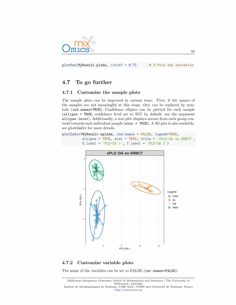
4.7 To go further4.7.1 Customize the sample plotsThe sample plots can be improved in various ways. First, if the names ofthe samples are not meaningful at this stage, they can be replaced by sym-bols (ind.names=TRUE). Confidence ellipses can be plotted for each sample(ellipse = TRUE, confidence level set to 95% by default, see the argumentellipse.level), Additionally, a star plot displays arrows from each group cen-troid towards each individual sample (star = TRUE). A 3D plot is also available,see plotIndiv for more details.plotIndiv(MyResult.splsda, ind.names = FALSE, legend=TRUE,

ellipse = TRUE, star = TRUE, title = 'sPLS-DA on SRBCT',X.label = 'PLS-DA 1', Y.label = 'PLS-DA 2')

sPLS−DA on SRBCT

0 5 10 15

−5

0

5

PLS−DA 1

PLS

−D

A 2

Legend

EWS

BL

NB

RMS

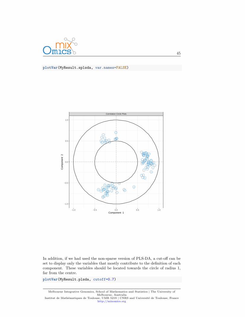
4.7.2 Customize variable plotsThe name of the variables can be set to FALSE (var.names=FALSE):



http://mixomics.org

45

plotVar(MyResult.splsda, var.names=FALSE)


−1.0 −0.5 0.0 0.5 1.0

−1.0

−0.5

0.0

0.5

1.0

Component 1

Com

pone

nt 2

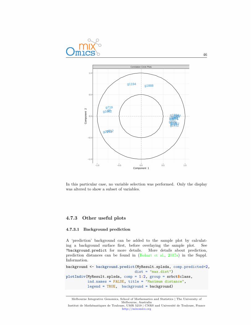
In addition, if we had used the non-sparse version of PLS-DA, a cut-off can beset to display only the variables that mostly contribute to the definition of eachcomponent. These variables should be located towards the circle of radius 1,far from the centre.plotVar(MyResult.plsda, cutoff=0.7)



http://mixomics.org

46

g1

g571

g719

g812

g875g906

g937g1007

g1067

g1082

g1167

g1194 g1888

g1894

g1932

g2253

g2276


−1.0 −0.5 0.0 0.5 1.0

−1.0

−0.5

0.0

0.5

1.0

Component 1

Com

pone

nt 2

In this particular case, no variable selection was performed. Only the displaywas altered to show a subset of variables.

4.7.3 Other useful plots

4.7.3.1 Background prediction

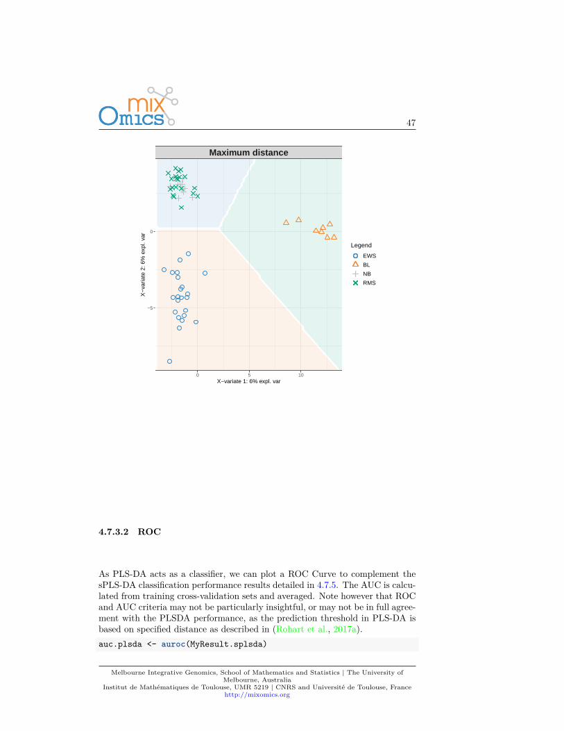
A ‘prediction’ background can be added to the sample plot by calculat-ing a background surface first, before overlaying the sample plot. See?background.predict for more details. More details about prediction,prediction distances can be found in (Rohart et al., 2017a) in the Suppl.Information.background <- background.predict(MyResult.splsda, comp.predicted=2,

dist = "max.dist")plotIndiv(MyResult.splsda, comp = 1:2, group = srbct$class,

ind.names = FALSE, title = "Maximum distance",legend = TRUE, background = background)



http://mixomics.org

47

Maximum distance

0 5 10

−5

0


X−

varia

te 2

: 6%

exp

l. va

r

Legend

EWS

BL

NB

RMS

4.7.3.2 ROC

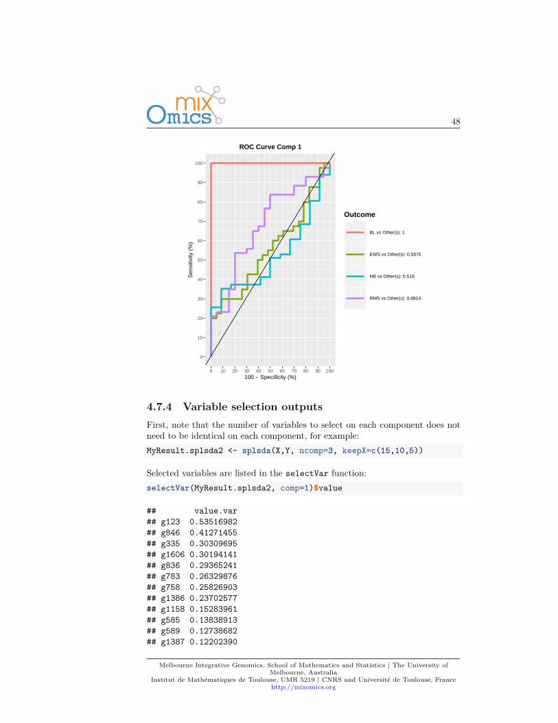
As PLS-DA acts as a classifier, we can plot a ROC Curve to complement thesPLS-DA classification performance results detailed in 4.7.5. The AUC is calcu-lated from training cross-validation sets and averaged. Note however that ROCand AUC criteria may not be particularly insightful, or may not be in full agree-ment with the PLSDA performance, as the prediction threshold in PLS-DA isbased on specified distance as described in (Rohart et al., 2017a).auc.plsda <- auroc(MyResult.splsda)



http://mixomics.org

48

0

10

20

30

40

50

60

70

80

90

100

0 10 20 30 40 50 60 70 80 90 100100 − Specificity (%)

Sen

sitiv

ity (

%)

Outcome

BL vs Other(s): 1

EWS vs Other(s): 0.5576

NB vs Other(s): 0.518

RMS vs Other(s): 0.6814

ROC Curve Comp 1

4.7.4 Variable selection outputsFirst, note that the number of variables to select on each component does notneed to be identical on each component, for example:MyResult.splsda2 <- splsda(X,Y, ncomp=3, keepX=c(15,10,5))

Selected variables are listed in the selectVar function:selectVar(MyResult.splsda2, comp=1)$value

## value.var## g123 0.53516982## g846 0.41271455## g335 0.30309695## g1606 0.30194141## g836 0.29365241## g783 0.26329876## g758 0.25826903## g1386 0.23702577## g1158 0.15283961## g585 0.13838913## g589 0.12738682## g1387 0.12202390



http://mixomics.org

49

## g1884 0.08458869## g1295 0.03150351## g1036 0.00224886

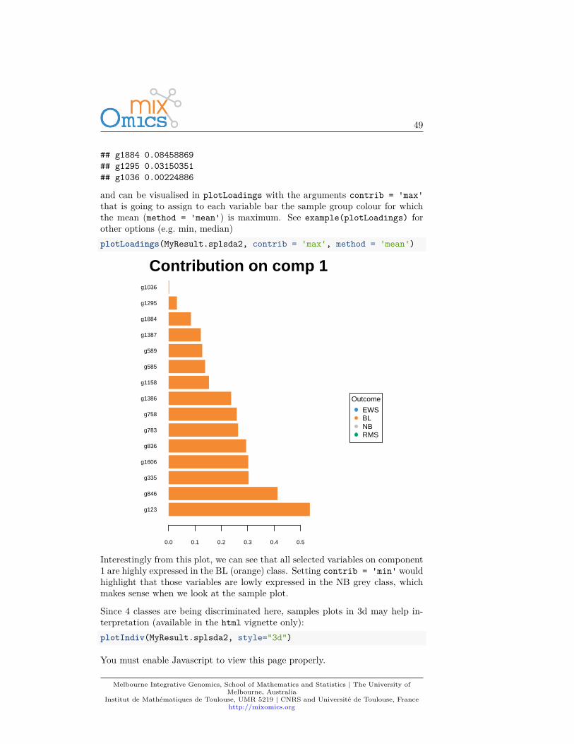
and can be visualised in plotLoadings with the arguments contrib = 'max'that is going to assign to each variable bar the sample group colour for whichthe mean (method = 'mean') is maximum. See example(plotLoadings) forother options (e.g. min, median)plotLoadings(MyResult.splsda2, contrib = 'max', method = 'mean')

g123

g846

g335

g1606

g836

g783

g758

g1386

g1158

g585

g589

g1387

g1884

g1295

g1036

0.0 0.1 0.2 0.3 0.4 0.5

Contribution on comp 1

Outcome

EWSBLNBRMS

Interestingly from this plot, we can see that all selected variables on component1 are highly expressed in the BL (orange) class. Setting contrib = 'min' wouldhighlight that those variables are lowly expressed in the NB grey class, whichmakes sense when we look at the sample plot.

Since 4 classes are being discriminated here, samples plots in 3d may help in-terpretation (available in the html vignette only):plotIndiv(MyResult.splsda2, style="3d")

You must enable Javascript to view this page properly.



http://mixomics.org

50

4.7.5 Tuning parameters and numerical outputsFor this set of methods, three parameters need to be chosen:

1 - The number of components to retain ncomp. The rule of thumb is usuallyK − 1 where K is the number of classes, but it is worth testing a few extracomponents.

2 - The number of variables keepX to select on each component for sparse PLS-DA,

3 - The prediction distance to evaluate the classification and prediction perfor-mance of PLS-DA.

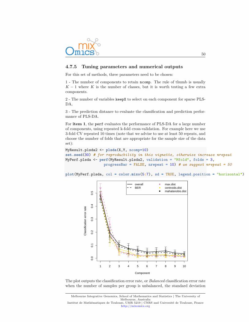
For item 1, the perf evaluates the performance of PLS-DA for a large numberof components, using repeated k-fold cross-validation. For example here we use3-fold CV repeated 10 times (note that we advise to use at least 50 repeats, andchoose the number of folds that are appropriate for the sample size of the dataset):MyResult.plsda2 <- plsda(X,Y, ncomp=10)set.seed(30) # for reproducbility in this vignette, otherwise increase nrepeatMyPerf.plsda <- perf(MyResult.plsda2, validation = "Mfold", folds = 3,

progressBar = FALSE, nrepeat = 10) # we suggest nrepeat = 50

plot(MyPerf.plsda, col = color.mixo(5:7), sd = TRUE, legend.position = "horizontal")

0.0

0.1

0.2

0.3

0.4

0.5

Component

Cla

ssifi

catio

n er

ror

rate

1 2 3 4 5 6 7 8 9 10

overallBER

max.distcentroids.distmahalanobis.dist

The plot outputs the classification error rate, or Balanced classification error ratewhen the number of samples per group is unbalanced, the standard deviation



http://mixomics.org

51

according to three prediction distances. Here we can see that for the BER andthe maximum distance, the best performance (i.e. low error rate) seems to beachieved for ncomp = 3.

In addition (item 3 for PLS-DA), the numerical outputs listed here can bereported as performance measures:MyPerf.plsda

#### Call:## perf.mixo_plsda(object = MyResult.plsda2, validation = "Mfold", folds = 3, nrepeat = 10, progressBar = FALSE)#### Main numerical outputs:## --------------------## Error rate (overall or BER) for each component and for each distance: see object$error.rate## Error rate per class, for each component and for each distance: see object$error.rate.class## Prediction values for each component: see object$predict## Classification of each sample, for each component and for each distance: see object$class## AUC values: see object$auc if auc = TRUE#### Visualisation Functions:## --------------------## plot

Regarding item 2, we now use tune.splsda to assess the optimal number ofvariables to select on each component. We first set up a grid of keepX valuesthat will be assessed on each component, one component at a time. Similar toabove we run 3-fold CV repeated 10 times with a maximum distance predictiondefined as above.list.keepX <- c(5:10, seq(20, 100, 10))list.keepX # to output the grid of values tested

## [1] 5 6 7 8 9 10 20 30 40 50 60 70 80 90 100set.seed(30) # for reproducbility in this vignette, otherwise increase nrepeattune.splsda.srbct <- tune.splsda(X, Y, ncomp = 3, # we suggest to push ncomp a bit more, e.g. 4

validation = 'Mfold',folds = 3, dist = 'max.dist', progressBar = FALSE,measure = "BER", test.keepX = list.keepX,nrepeat = 10) # we suggest nrepeat = 50

We can then extract the classification error rate averaged across all folds andrepeats for each tested keepX value, the optimal number of components (see?tune.splsda for more details), the optimal number of variables to select percomponent which is summarised in a plot where the diamond indicated theoptimal keepX value:



http://mixomics.org

52

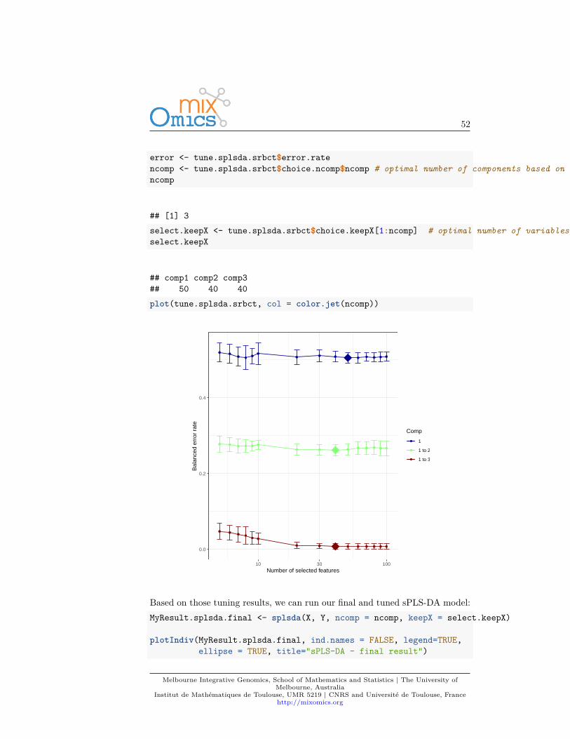
error <- tune.splsda.srbct$error.ratencomp <- tune.splsda.srbct$choice.ncomp$ncomp # optimal number of components based on t-tests on the error ratencomp

## [1] 3select.keepX <- tune.splsda.srbct$choice.keepX[1:ncomp] # optimal number of variables to selectselect.keepX

## comp1 comp2 comp3## 50 40 40plot(tune.splsda.srbct, col = color.jet(ncomp))

0.0

0.2

0.4

10 30 100Number of selected features

Bal

ance

d er

ror

rate

Comp

1

1 to 2

1 to 3

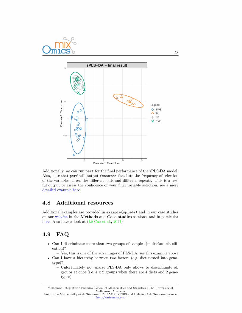
Based on those tuning results, we can run our final and tuned sPLS-DA model:MyResult.splsda.final <- splsda(X, Y, ncomp = ncomp, keepX = select.keepX)

plotIndiv(MyResult.splsda.final, ind.names = FALSE, legend=TRUE,ellipse = TRUE, title="sPLS-DA - final result")



http://mixomics.org

53

sPLS−DA − final result

0 5 10 15

−5

0

5


X−

varia

te 2

: 6%

exp

l. va

r

Legend

EWS

BL

NB

RMS

Additionally, we can run perf for the final performance of the sPLS-DA model.Also, note that perf will output features that lists the frequency of selectionof the variables across the different folds and different repeats. This is a use-ful output to assess the confidence of your final variable selection, see a moredetailed example here.

4.8 Additional resourcesAdditional examples are provided in example(splsda) and in our case studieson our website in the Methods and Case studies sections, and in particularhere. Also have a look at (Lê Cao et al., 2011)

4.9 FAQ• Can I discriminate more than two groups of samples (multiclass classifi-

cation)?– Yes, this is one of the advantages of PLS-DA, see this example above

• Can I have a hierarchy between two factors (e.g. diet nested into geno-type)?

– Unfortunately no, sparse PLS-DA only allows to discriminate allgroups at once (i.e. 4 x 2 groups when there are 4 diets and 2 geno-types)



http://mixomics.org/case-studies/splsda-srbct/


http://mixomics.org/case-studies/splsda-srbct/

http://mixomics.org

54

• Can I have missing values in my data?– Yes in the X data set, but you won’t be able to do any prediction

(i.e. tune, perf, predict)– No in the Y factor



http://mixomics.org

55

Chapter 5

Projection to LatentStructure (PLS)

PLS overview

PLS

Quantitative

5.1 Biological questionI would like to integrate two data sets measured on the same samples by extractingcorrelated information, or by highlighing commonalities between data sets.



http://mixomics.org

56

5.2 The nutrimouse studyThe nutrimouse study contains the expression levels of genes potentially in-volved in nutritional problems and the concentrations of hepatic fatty acids forforty mice. The data sets come from a nutrigenomic study in the mouse fromour collaborator (Martin et al., 2007), in which the effects of five regimens withcontrasted fatty acid compositions on liver lipids and hepatic gene expressionin mice were considered. Two sets of variables were measured on 40 mice:

• gene: the expression levels of 120 genes measured in liver cells, selectedamong (among about 30,000) as potentially relevant in the context of thenutrition study. These expressions come from a nylon microarray withradioactive labelling.

• lipid: concentration (in percentage) of 21 hepatic fatty acids measuredby gas chromatography.

• diet: a 5-level factor. Oils used for experimental diets preparation werecorn and colza oils (50/50) for a reference diet (REF), hydrogenated co-conut oil for a saturated fatty acid diet (COC), sunflower oil for an Omega6fatty acid-rich diet (SUN), linseed oil for an Omega3-rich diet (LIN) andcorn/colza/enriched fish oils for the FISH diet (43/43/14).

• genotype 2-levels factor indicating either wild-type (WT) and PPARα -/-(PPAR).

More details can be found in ?nutrimouse.

To illustrate sparse PLS, we will integrate the gene expression levels (gene) withthe concentrations of hepatic fatty acids (lipid).

5.3 Principle of PLSPartial Least Squares (PLS) regression (Wold, 1966; Wold et al., 2001) is a mul-tivariate methodology which relates (integrates) two data matrices X (e.g. tran-scriptomics) and Y (e.g. lipids). PLS goes beyond traditional multiple regres-sion by modelling the structure of both matrices. Unlike traditional multipleregression models, it is not limited to uncorrelated variables. One of the manyadvantages of PLS is that it can handle many noisy, collinear (correlated) andmissing variables and can also simultaneously model several response variablesin Y.

PLS is a multivariate projection-based method that can address different typesof integration problems. Its flexibility is the reason why it is the backbone ofmost methods in mixOmics. PLS is computationally very efficient when thenumber of variables p + q >> n the number of samples. It performs succes-sive local regressions that avoid computational issues due to the inversion oflarge singular covariance matrices. Unlike PCA which maximizes the varianceof components from a single data set, PLS maximizes the covariance between



http://mixomics.org

57

components from two data sets. The mathematical concepts of covariance andcorrelation are similar, but the covariance is an unbounded measure and covari-ance has a unit measure (see 1.2.1). In PLS, a linear combination of variablesis called latent variables or latent components. The weight vectors used to cal-culate the linear combinations are called the loading vectors. Latent variablesand loading vectors are thus associated and come in pairs from each of the twodata sets being integrated.

5.4 Principle of sparse PLSEven though PLS is highly efficient in a high dimensional context, the inter-pretability of PLS needed to be improved. sPLS has been recently developed byour team to perform simultaneous variable selection in both data sets X and Ydata sets, by including LASSO ℓ1 penalizations in PLS on each pair of loadingvectors (Lê Cao et al., 2008).

5.5 Inputs and outputsWe consider the data input matrices: X is a n×p data matrix and Y a n×q datamatrix, where n the number of samples (individuals), p and q are the numberof variables in each data set. PLS main outputs are:

• A set of components, also called latent variables associated to each dataset. There are as many components as the chosen dimension of the PLS.

• A set of loading vectors, which are coefficients assigned to each variableto define each component. These coefficients indicate the importance ofeach variable in PLS. Importantly, each loading vector is associated to aparticular component. Loading vectors are obtained so that the covariancebetween a linear combination of the variables from X (the X-component)and from Y (the Y -component) is maximised.

• A list of selected variables from both X and Y and associated to eachcomponent if sPLS is applied.

5.6 Set up the dataWe first set up the data as X expression matrix and Y as the lipid abundancematrix. We also check that the dimensions are correct and match:library(mixOmics)data(nutrimouse)X <- nutrimouse$geneY <- nutrimouse$lipiddim(X); dim(Y)



http://mixomics.org

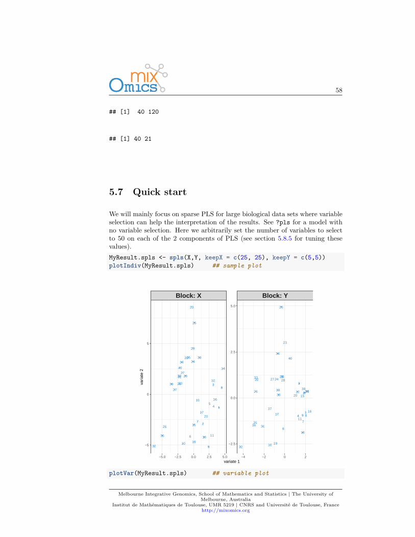
58

## [1] 40 120

## [1] 40 21

5.7 Quick start

We will mainly focus on sparse PLS for large biological data sets where variableselection can help the interpretation of the results. See ?pls for a model withno variable selection. Here we arbitrarily set the number of variables to selectto 50 on each of the 2 components of PLS (see section 5.8.5 for tuning thesevalues).MyResult.spls <- spls(X,Y, keepX = c(25, 25), keepY = c(5,5))plotIndiv(MyResult.spls) ## sample plot

1

2

3

45

6

7

8

910

11

12

13

14

15

16

17

1819

20

21

22

23

24

25

26

2728

29

30

31

32

33

3435

36

37

38

39

40

1

2

3

4

5

6

7

89

10

11

12 131415

1617

18

19

20

21

22

23

24

25

26

27 2829

30

31

32

33

34

35

36

37

3839

40

Block: X Block: Y

−5.0 −2.5 0.0 2.5 5.0 −4 −2 0 2

−2.5

0.0

2.5

5.0

−5

0

5

variate 1

varia

te 2

plotVar(MyResult.spls) ## variable plot



http://mixomics.org

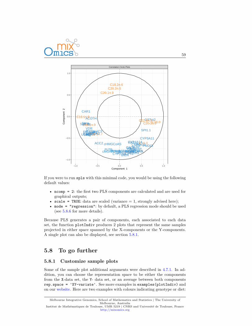
59

ACBPACC2

ACOTH

ALDH3AOX

BIENBSEP

CACP

CAR1

CBS

CPT2CYP27a1

CYP3A11

CYP4A10CYP4A14FAS

FAT

GKGSTa

GSTpi2

HPNCLL.FABP

Lpin2

MCAD

MDR2

MS

Ntcp

PDK4

PECIPLTP

PMDCI

RXRaRXRg1SHP1

SIAT4c

SPI1.1

SR.BI

THIOLTpalphaTpbeta

UCP2

VDRWaf1apoC3

cHMGCoAS

cMOAT

eif2g

mHMGCoAS

C16.0

C18.0

C16.1n.9

C18.1n.9

C18.1n.7

C20.1n.9

C18.2n.6C20.2n.6

C20.3n.6C22.6n.3


−1.0 −0.5 0.0 0.5 1.0

−1.0

−0.5

0.0

0.5

1.0

Component 1

Com

pone

nt 2

If you were to run spls with this minimal code, you would be using the followingdefault values:


• scale = TRUE: data are scaled (variance = 1, strongly advised here);• mode = "regression": by default, a PLS regression mode should be used

(see 5.8.6 for more details).

Because PLS generates a pair of components, each associated to each dataset, the function plotIndiv produces 2 plots that represent the same samplesprojected in either space spanned by the X-components or the Y-components.A single plot can also be displayed, see section 5.8.1.

5.8 To go further5.8.1 Customize sample plotsSome of the sample plot additional arguments were described in 4.7.1. In ad-dition, you can choose the representation space to be either the componentsfrom the X-data set, the Y- data set, or an average between both componentsrep.space = 'XY-variate'. See more examples in examples(plotIndiv) andon our website. Here are two examples with colours indicating genotype or diet:



http://mixomics.org/graphics/sample-plots/

http://mixomics.org

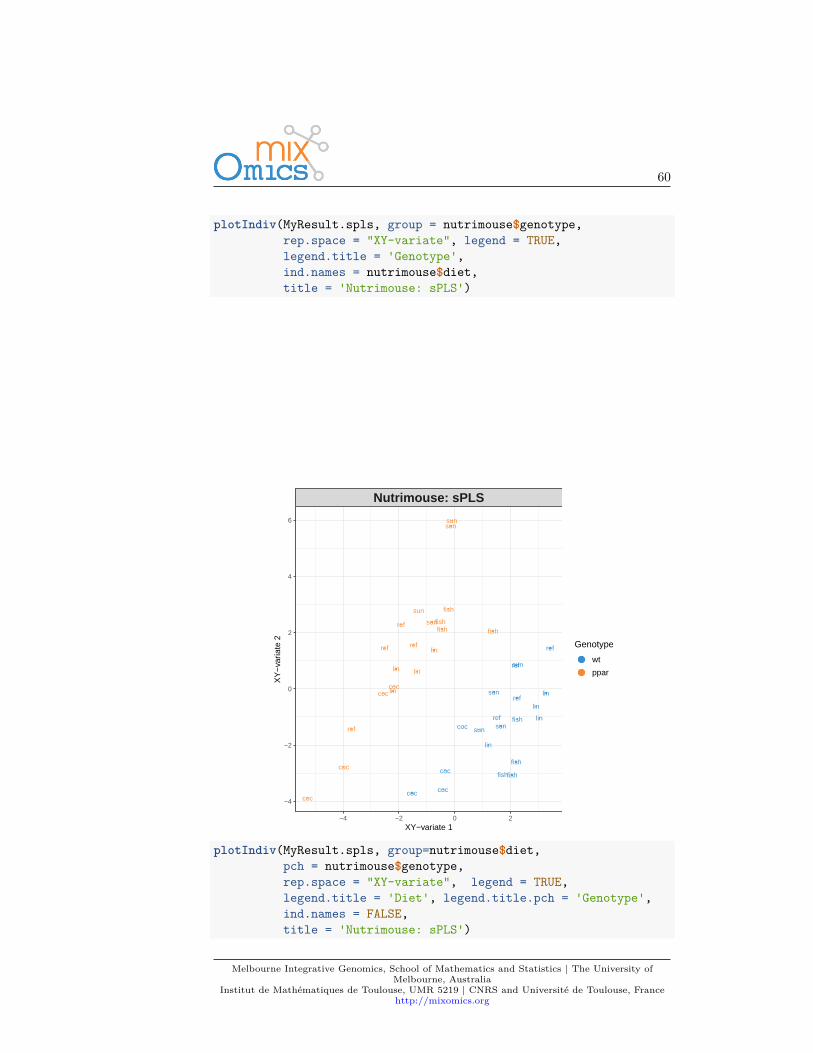
60

plotIndiv(MyResult.spls, group = nutrimouse$genotype,rep.space = "XY-variate", legend = TRUE,legend.title = 'Genotype',ind.names = nutrimouse$diet,title = 'Nutrimouse: sPLS')

linsun

sun

fish

ref

coc

lin

lin

fish

coc

fish

ref

sun

ref

sun

lin

coc

fish

coc

ref

coc

ref

sun

fish

sun

ref

reflin

fish

lin

coc

coc

ref

sun

fish

coc

lin

fish

lin

sun

Nutrimouse: sPLS

−4 −2 0 2

−4

−2

0

2

4

6

XY−variate 1

XY

−va

riate

2 Genotype

wt

ppar

plotIndiv(MyResult.spls, group=nutrimouse$diet,pch = nutrimouse$genotype,rep.space = "XY-variate", legend = TRUE,legend.title = 'Diet', legend.title.pch = 'Genotype',ind.names = FALSE,title = 'Nutrimouse: sPLS')



http://mixomics.org

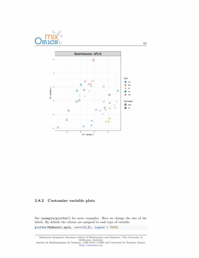
61

Nutrimouse: sPLS

−4 −2 0 2

−4

−2

0

2

4

6

XY−variate 1

XY

−va

riate

2

Diet

coc

fish

lin

ref

sun

Genotype

ppar

wt

5.8.2 Customize variable plots

See (example(plotVar)) for more examples. Here we change the size of thelabels. By default the colours are assigned to each type of variable.plotVar(MyResult.spls, cex=c(3,2), legend = TRUE)



http://mixomics.org

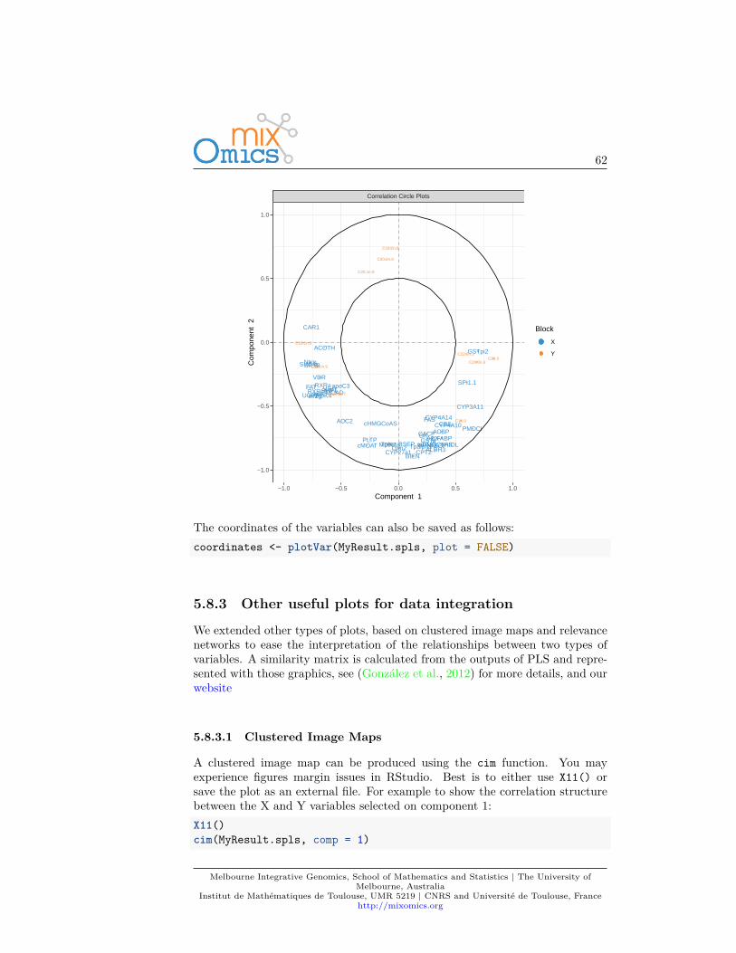
62

ACBP

ACC2

ACOTH

ALDH3

AOX

BIEN

BSEP

CACP

CAR1

CBS

CPT2CYP27a1

CYP3A11

CYP4A10CYP4A14FAS

FAT

GKGSTa

GSTpi2

HPNCLL.FABP

Lpin2

MCAD

MDR2

MS

Ntcp

PDK4

PECIPLTP

PMDCI

RXRaRXRg1SHP1

SIAT4c

SPI1.1

SR.BI

THIOLTpalphaTpbeta

UCP2

VDR

Waf1apoC3

cHMGCoAS

cMOAT

eif2g

mHMGCoAS

C16.0

C18.0

C16.1n.9

C18.1n.9

C18.1n.7

C20.1n.9

C18.2n.6

C20.2n.6

C20.3n.6

C22.6n.3


−1.0 −0.5 0.0 0.5 1.0

−1.0

−0.5

0.0

0.5

1.0

Component 1

Com

pone

nt 2 Block

X

Y

The coordinates of the variables can also be saved as follows:coordinates <- plotVar(MyResult.spls, plot = FALSE)

5.8.3 Other useful plots for data integration

We extended other types of plots, based on clustered image maps and relevancenetworks to ease the interpretation of the relationships between two types ofvariables. A similarity matrix is calculated from the outputs of PLS and repre-sented with those graphics, see (González et al., 2012) for more details, and ourwebsite

5.8.3.1 Clustered Image Maps

A clustered image map can be produced using the cim function. You mayexperience figures margin issues in RStudio. Best is to either use X11() orsave the plot as an external file. For example to show the correlation structurebetween the X and Y variables selected on component 1:X11()cim(MyResult.spls, comp = 1)



http://mixomics.org/graphics/variable-plots/

http://mixomics.org

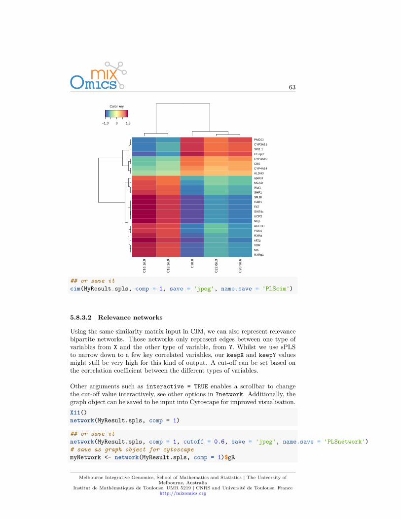
63

−1.3 0 1.3

Color key

C16

.1n.

9

C18

.1n.

9

C18

.0

C22

.6n.

3

C20

.3n.

6

RXRg1

MS

VDR

eif2g

RXRa

PDK4

ACOTH

Ntcp

UCP2

SIAT4c

FAT

CAR1

SR.BI

SHP1

Waf1

MCAD

apoC3

ALDH3

CYP4A14

CBS

CYP4A10

GSTpi2

SPI1.1

CYP3A11

PMDCI

## or save itcim(MyResult.spls, comp = 1, save = 'jpeg', name.save = 'PLScim')

5.8.3.2 Relevance networks

Using the same similarity matrix input in CIM, we can also represent relevancebipartite networks. Those networks only represent edges between one type ofvariables from X and the other type of variable, from Y. Whilst we use sPLSto narrow down to a few key correlated variables, our keepX and keepY valuesmight still be very high for this kind of output. A cut-off can be set based onthe correlation coefficient between the different types of variables.

Other arguments such as interactive = TRUE enables a scrollbar to changethe cut-off value interactively, see other options in ?network. Additionally, thegraph object can be saved to be input into Cytoscape for improved visualisation.X11()network(MyResult.spls, comp = 1)

## or save itnetwork(MyResult.spls, comp = 1, cutoff = 0.6, save = 'jpeg', name.save = 'PLSnetwork')# save as graph object for cytoscapemyNetwork <- network(MyResult.spls, comp = 1)$gR



http://mixomics.org

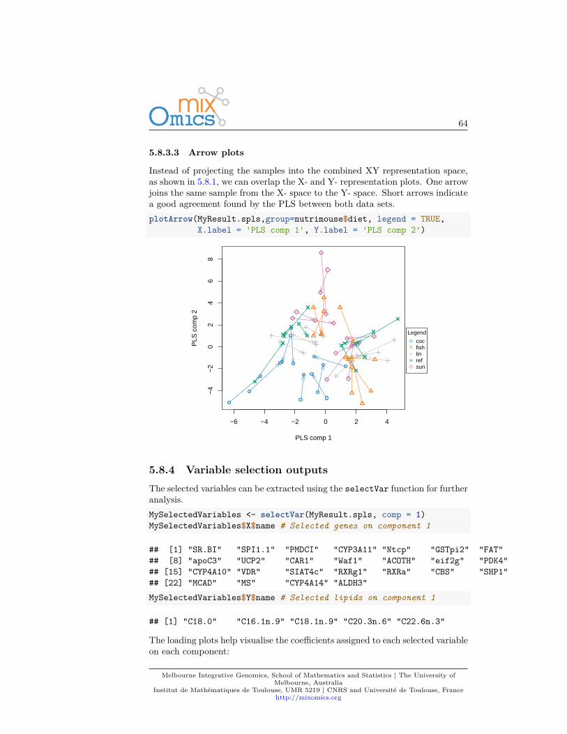
64

5.8.3.3 Arrow plots

Instead of projecting the samples into the combined XY representation space,as shown in 5.8.1, we can overlap the X- and Y- representation plots. One arrowjoins the same sample from the X- space to the Y- space. Short arrows indicatea good agreement found by the PLS between both data sets.plotArrow(MyResult.spls,group=nutrimouse$diet, legend = TRUE,

X.label = 'PLS comp 1', Y.label = 'PLS comp 2')

−6 −4 −2 0 2 4

−4

−2

02

46

8

PLS comp 1

PLS

com

p 2

Legend

cocfishlinrefsun

5.8.4 Variable selection outputsThe selected variables can be extracted using the selectVar function for furtheranalysis.MySelectedVariables <- selectVar(MyResult.spls, comp = 1)MySelectedVariables$X$name # Selected genes on component 1

## [1] "SR.BI" "SPI1.1" "PMDCI" "CYP3A11" "Ntcp" "GSTpi2" "FAT"## [8] "apoC3" "UCP2" "CAR1" "Waf1" "ACOTH" "eif2g" "PDK4"## [15] "CYP4A10" "VDR" "SIAT4c" "RXRg1" "RXRa" "CBS" "SHP1"## [22] "MCAD" "MS" "CYP4A14" "ALDH3"MySelectedVariables$Y$name # Selected lipids on component 1

## [1] "C18.0" "C16.1n.9" "C18.1n.9" "C20.3n.6" "C22.6n.3"

The loading plots help visualise the coefficients assigned to each selected variableon each component:



http://mixomics.org

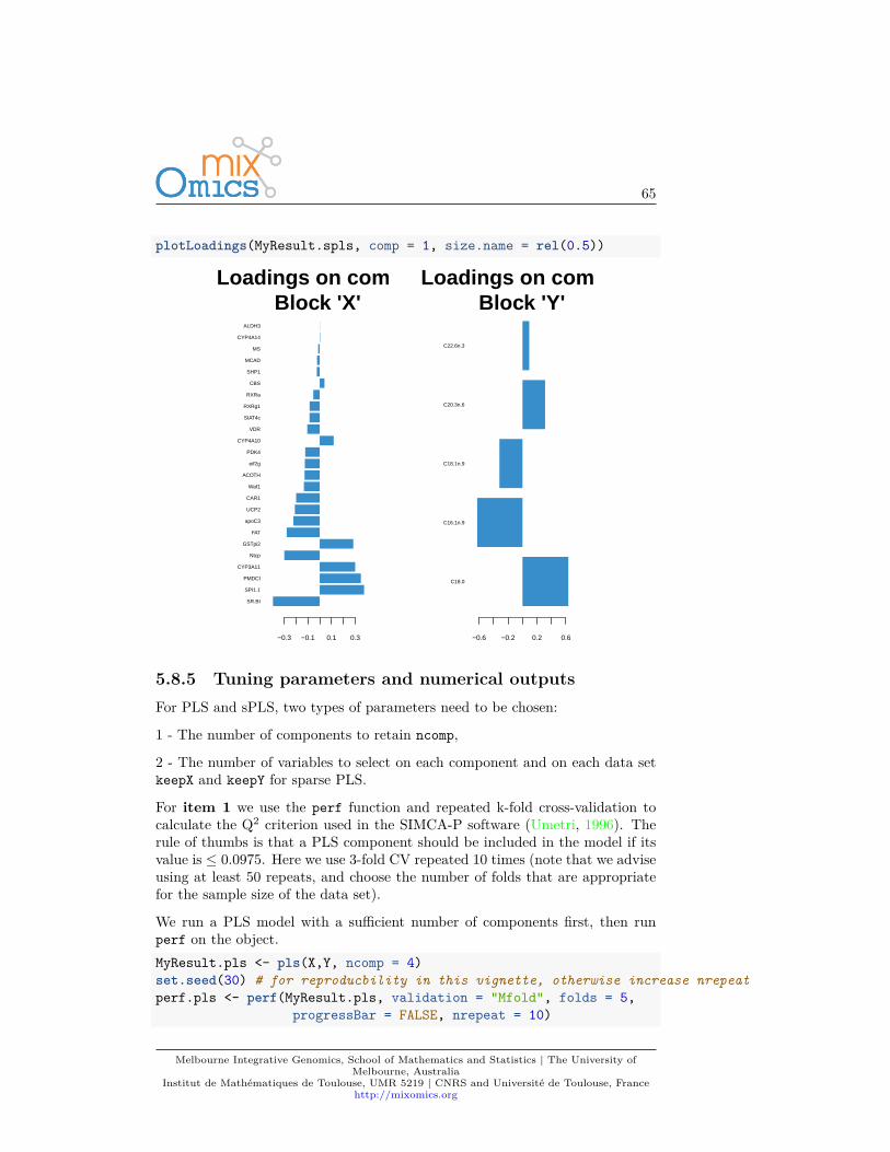
65

plotLoadings(MyResult.spls, comp = 1, size.name = rel(0.5))

SR.BI

SPI1.1

PMDCI

CYP3A11

Ntcp

GSTpi2

FAT

apoC3

UCP2

CAR1

Waf1

ACOTH

eif2g

PDK4

CYP4A10

VDR

SIAT4c

RXRg1

RXRa

CBS

SHP1

MCAD

MS

CYP4A14

ALDH3

−0.3 −0.1 0.1 0.3

Loadings on comp 1Block 'X'

C18.0

C16.1n.9

C18.1n.9

C20.3n.6

C22.6n.3

−0.6 −0.2 0.2 0.6

Loadings on comp 1Block 'Y'

5.8.5 Tuning parameters and numerical outputsFor PLS and sPLS, two types of parameters need to be chosen:

1 - The number of components to retain ncomp,

2 - The number of variables to select on each component and on each data setkeepX and keepY for sparse PLS.

For item 1 we use the perf function and repeated k-fold cross-validation tocalculate the Q2 criterion used in the SIMCA-P software (Umetri, 1996). Therule of thumbs is that a PLS component should be included in the model if itsvalue is ≤ 0.0975. Here we use 3-fold CV repeated 10 times (note that we adviseusing at least 50 repeats, and choose the number of folds that are appropriatefor the sample size of the data set).

We run a PLS model with a sufficient number of components first, then runperf on the object.MyResult.pls <- pls(X,Y, ncomp = 4)set.seed(30) # for reproducbility in this vignette, otherwise increase nrepeatperf.pls <- perf(MyResult.pls, validation = "Mfold", folds = 5,

progressBar = FALSE, nrepeat = 10)



http://mixomics.org

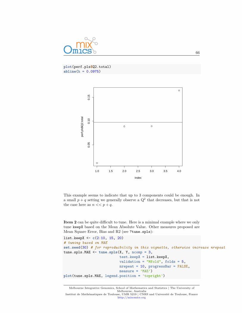
66

plot(perf.pls$Q2.total)abline(h = 0.0975)

1.0 1.5 2.0 2.5 3.0 3.5 4.0

0.05

0.10

0.15

Index

perf

.pls

$Q2.

tota

l

This example seems to indicate that up to 3 components could be enough. Ina small p + q setting we generally observe a Q2 that decreases, but that is notthe case here as n << p + q.

Item 2 can be quite difficult to tune. Here is a minimal example where we onlytune keepX based on the Mean Absolute Value. Other measures proposed areMean Square Error, Bias and R2 (see ?tune.spls):list.keepX <- c(2:10, 15, 20)# tuning based on MAEset.seed(30) # for reproducbility in this vignette, otherwise increase nrepeattune.spls.MAE <- tune.spls(X, Y, ncomp = 3,

test.keepX = list.keepX,validation = "Mfold", folds = 5,nrepeat = 10, progressBar = FALSE,measure = 'MAE')

plot(tune.spls.MAE, legend.position = 'topright')



http://mixomics.org

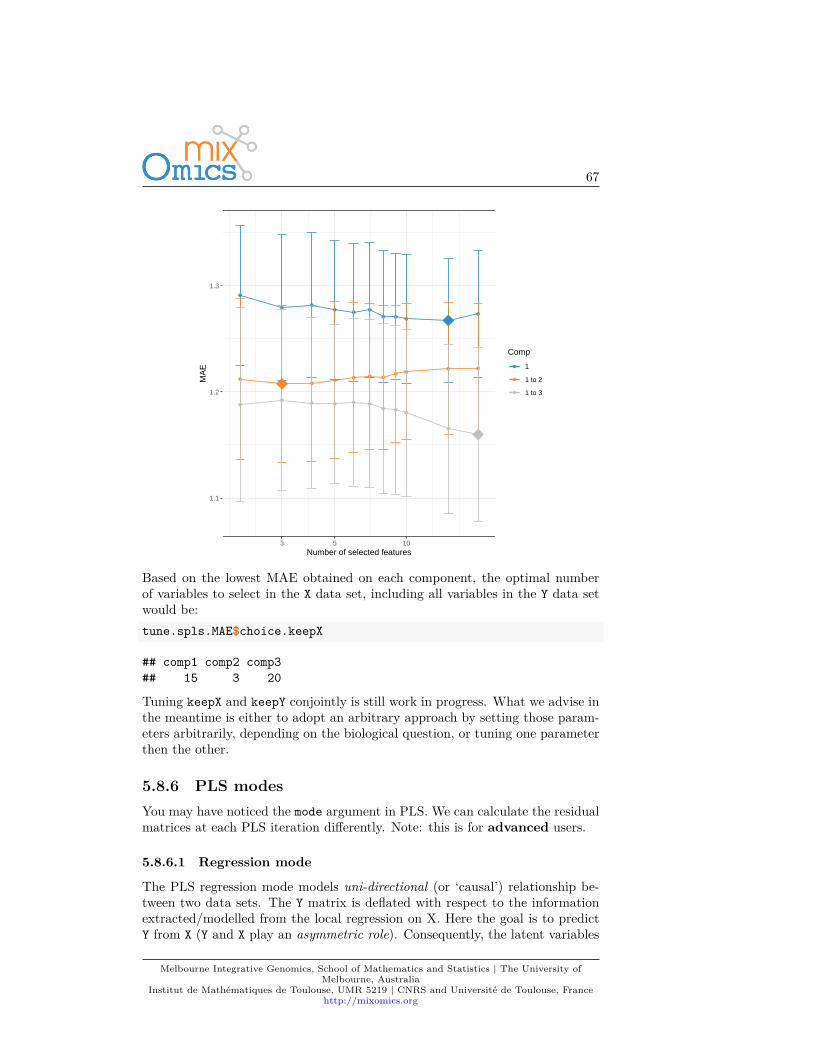
67

1.1

1.2

1.3

3 5 10Number of selected features

MA

E

Comp

1

1 to 2

1 to 3

Based on the lowest MAE obtained on each component, the optimal numberof variables to select in the X data set, including all variables in the Y data setwould be:tune.spls.MAE$choice.keepX

## comp1 comp2 comp3## 15 3 20

Tuning keepX and keepY conjointly is still work in progress. What we advise inthe meantime is either to adopt an arbitrary approach by setting those param-eters arbitrarily, depending on the biological question, or tuning one parameterthen the other.

5.8.6 PLS modesYou may have noticed the mode argument in PLS. We can calculate the residualmatrices at each PLS iteration differently. Note: this is for advanced users.

5.8.6.1 Regression mode

The PLS regression mode models uni-directional (or ‘causal’) relationship be-tween two data sets. The Y matrix is deflated with respect to the informationextracted/modelled from the local regression on X. Here the goal is to predictY from X (Y and X play an asymmetric role). Consequently, the latent variables



http://mixomics.org

68

computed to predict Y from X are different from those computed to predict Xfrom Y. More details about the model can be found in[ Appendix (Lê Cao et al.,2008).

PLS regression mode, also called PLS2, is commonly applied for the analysisof biological data (Boulesteix and Strimmer, 2005; Bylesjö et al., 2007) due tothe biological assumptions or the biological dogma. In general, the number ofvariables in Y to predict are fewer in number than the predictors in X.

5.8.6.2 Canonical mode

Similar to a Canonical Correlation Analysis (CCA) framework, this mode isused to model a bi-directional (or symmetrical) relationship between the twodata sets. The Y matrix is deflated with respect to the information extractedor modelled from the local regression on Y. Here X and Y play a symmetric roleand the goal is similar to CCA. More details about the model can be found in(Lê Cao et al., 2009).

PLS canonical mode is not well known (yet), but is applicable when there isno a priori relationship between the two data sets, or in place of CCA butwhen variable selection is required in large data sets. In (Lê Cao et al., 2009),we compared the measures of the same biological samples on different types ofmicroarrays, cDNA and Affymetrix arrays, to highlight complementary infor-mation at the transcripts levels. Note however that for this mode we do notprovide any tuning function.

5.8.6.3 Other modes

The ‘invariant’ mode performs a redundancy analysis, where the Y matrix is notdeflated. The ‘classic’ mode is similar to a regression mode. It gives identicalresults for the variates and loadings associated to the X data set, but differencesfor the loadings vectors associated to the Y data set (different normalisationsare used). Classic mode is the PLS2 model as defined by (Tenenhaus, 1998),Chap 9.

5.8.6.4 Difference between PLS modes

For the first PLS dimension, all PLS modes will output the same results interms of latent variables and loading vectors. After the first dimension, thesevectors will differ, as the matrices are deflated differently.

5.9 Additional resourcesAdditional examples are provided in example(spls) and in our case studies onour website in the Methods and Case studies sections, see also (Lê Cao et al.,2008, 2009).




http://mixomics.org

69

5.10 FAQ• Can PLS handle missing values?

– Yes it can, but only for the learning / training analysis. Predictionwith perf or tune is not possible with missing values.

• Can PLS deal with more than 2 data sets?– sPLS can only deal with 2 data sets but see DIABLO (Chapter 6) for

multi-block analyses• What are the differences between sPLS and Canonical Correlation Anal-

ysis (CCA, see ?rcca in mixOmics)?– CCA maximises the correlation between components; PLS maximises

the covariance– Both methods give similar results if the components are scaled, but

the underlying algorithms are different:∗ CCA calculates all component at once, there is no deflation∗ PLS has different deflation mode

– sparse PLS selects variables, CCA cannot perform variable selection• Can I perform PLS with more variables than observations?

– Yes, and sparse PLS is particularly useful to identify sets of variablesthat play a role in explaining the relationship between two data sets.

• Can I perform PLS with 2 data sets that are highly unbalanced (thousandsof variables in one data set and less than 10 in the other?

– Yes! Even if you performed sPLS to select variables in one data set(or both), you can still control the number of variables selected withkeepX.



http://mixomics.org

70



http://mixomics.org

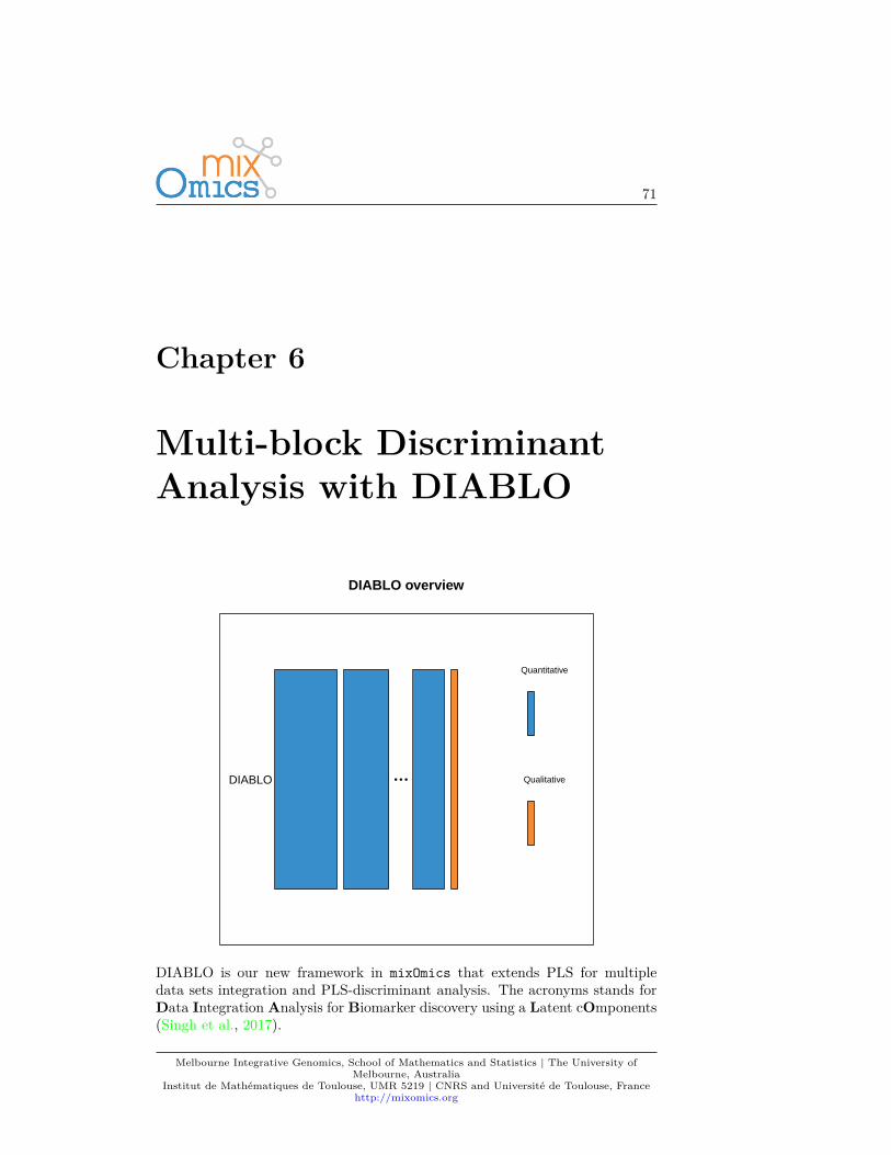
71

Chapter 6

Multi-block DiscriminantAnalysis with DIABLO

DIABLO overview

DIABLO

Quantitative

Qualitative

DIABLO is our new framework in mixOmics that extends PLS for multipledata sets integration and PLS-discriminant analysis. The acronyms stands forData Integration Analysis for Biomarker discovery using a Latent cOmponents(Singh et al., 2017).



http://mixomics.org

72

6.1 Biological questionI would like to identify a highly correlated multi-omics signature discriminatingknown groups of samples.

6.2 The breast.TCGA studyHuman breast cancer is a heterogeneous disease in terms of molecular alter-ations, cellular composition, and clinical outcome. Breast tumours can be clas-sified into several subtypes, according to levels of mRNA expression [Sorlie et al.(2001). Here we consider a subset of data generated by The Cancer GenomeAtlas Network (Cancer Genome Atlas Network et al., 2012). For the package,data were normalised and drastically prefiltered for illustrative purposes but DI-ABLO can handle larger data sets, see (Rohart et al., 2017a) Table 2. The datawere divided into a training set with a subset of 150 samples from the mRNA,miRNA and proteomics data, and a test set including 70 samples, but only withmRNA and miRNA data (proteomics missing). The aim of this integrativeanalysis is to identify a highly correlated multi-omics signature discriminatingthe breast cancer subtypes Basal, Her2 and LumA.

The breast.TCGA is a list containing training and test sets of omics datadata.train and data.test which both include:

• miRNA: a data frame with 150 (70) rows and 184 columns in the training(test) data set for the miRNA expression levels.

• mRNA: a data frame with 150 (70) rows and 520 columns in the training(test) data set for the mRNA expression levels.

• protein: a data frame with 150 rows and 142 columns in the trainingdata set only for the protein abundance.

• subtype: a factor indicating the breast cancer subtypes in the training(length of 150) and test (length of 70) sets.

More details can be found in ?breast.TCGA.

To illustrate DIABLO, we will integrate the expression levels of miRNA, mRNAand the abundance of proteins while discriminating the subtypes of breast can-cer, then predict the subtypes of the test samples in the test set.

6.3 Principle of DIABLOThe core DIABLO method extends Generalised Canonical Correlation Analy-sis (Tenenhaus and Tenenhaus, 2011), which contrary to what its name sug-gests, generalises PLS for multiple matching datasets, and the sparse sGCCAmethod (Tenenhaus et al., 2014). Starting from the R package RGCCA, weextended these methods for different types of analyses, including unsupervised



http://mixomics.org

73

N-integration (block.pls, block.spls) and supervised analyses (block.plsda,block.splsda).

The aim of N-integration with our sparse methods is to identify correlated (orco-expressed) variables measured on heterogeneous data sets which also explainthe categorical outcome of interest (supervised analysis). The multiple dataintegration task is not trivial, as the analysis can be strongly affected by thevariation between manufacturers or omics technological platforms despite beingmeasured on the same biological samples. Before you embark on data integra-tion, we strongly suggest individual or paired analyses with sPLS-DA and PLSto first understand the major sources of variation in each data set and to guidethe integration process.

More methodological details can be found in (Singh et al., 2017).

6.4 Inputs and outputsWe consider as input a list X of data frames with n rows (the number of samples)and a different number of variations in each data frame. Y is a factor vectorof length n that indicates the class of each sample. Internally and similar toPLS-DA in Chapter 4 it will be coded as a dummy matrix.

DIABLO main outputs are:

• A set of components, also called latent variables associated to each dataset. There are as many components as the chosen dimension of DIABLO.

• A set of loading vectors, which are coefficients assigned to each vari-able to define each component. These coefficients indicate the importanceof each variable in DIABLO. Importantly, each loading vector is associ-ated to a particular component. Loading vectors are obtained so thatthe covariance between a linear combination of the variables from X (theX-component) and from Y (the Y -component) is maximised.

• A list of selected variables from each data set and associated to eachcomponent if sparse DIABLO is applied.

6.5 Set up the dataWe first set up the input data as a list of data frames X expression matrix andY as a factor indicating the class membership of each sample. Each data framein X should be named consistently to match with the keepX parameter.

We check that the dimensions are correct and match. We then set up arbitrarilythe number of variables keepX that we wish to select in each data set and eachcomponent.



http://mixomics.org

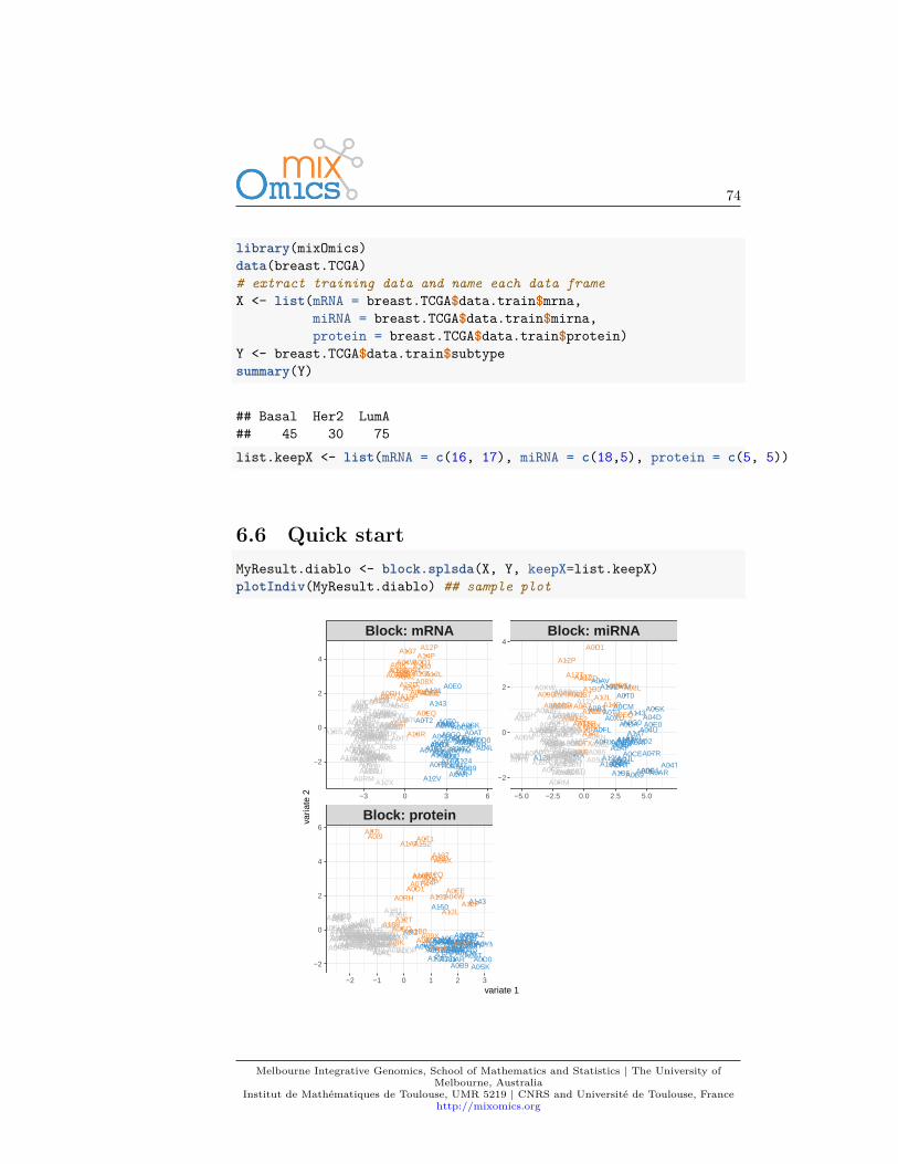
74

library(mixOmics)data(breast.TCGA)# extract training data and name each data frameX <- list(mRNA = breast.TCGA$data.train$mrna,

miRNA = breast.TCGA$data.train$mirna,protein = breast.TCGA$data.train$protein)

Y <- breast.TCGA$data.train$subtypesummary(Y)

## Basal Her2 LumA## 45 30 75list.keepX <- list(mRNA = c(16, 17), miRNA = c(18,5), protein = c(5, 5))

6.6 Quick startMyResult.diablo <- block.splsda(X, Y, keepX=list.keepX)plotIndiv(MyResult.diablo) ## sample plot

A0FJ

A13EA0G0

A0SX

A143

A0DA

A0B3

A0I2A0RT

A131

A124A1B6

A1AZA0YM

A04PA04TA0AT

A0AL

A0CEA07RA0FL

A150

A0E0

A0U4

A0XU

A0AV

A0AR

A0RX A0D2

A0CM

A0WX

A0T0A0T2

A04UA0JL

A147

A0B9A1AI

A14X

A12V

A1AY A0D0

A0SK

A128

A04D

A0A7

A094 A12LA0I9

A0EE

A135A152

A18P

A18R

A08XA0TXA09X

A1AT

A12Q

A12TA0RHA07I

A04W

A12P

A0EQ

A0D1A09G A1B0

A14P

A0T1

A137

A13ZA08L

A0IK

A12D

A0XNA0B0

A18S

A0CS

A0EI

A0IO

A0T6

A1AU

A07Z

A0XS

A1BD

A08T

A12Y

A0J5A18F

A0AS

A0DV

A140

A0SUA12A

A0RM

A0AZ

A0EW

A0XW

A12B

A0BPA0RG A0T7

A08AA0DK

A0SH

A18N

A06P

A15L

A0YLA1AL

A133

A086

A0I8

A0EA

A09A

A0DSA1B1

A0X0

A1AP

A0W5

A0JFA1AV

A0RO

A08Z

A0RVA0DP

A0EX

A15R

A0FD

A0ESA0BMA0EU

A12X

A146

A0CDA0BQ

A04A

A0CT

A0TZ

A03L

A1AK

A0E1A0H7

A0FS

A0BS

A08O

A12H

A15E

A0W4

A0FJA13EA0G0

A0SX

A143

A0DAA0B3A0I2

A0RTA131

A124A1B6

A1AZA0YMA04P A04T

A0AT

A0ALA0CEA07R

A0FL

A150

A0E0

A0U4A0XUA0AV

A0AR

A0RXA0D2A0CM

A0WXA0T0A0T2A04UA0JLA147

A0B9

A1AIA14X

A12V

A1AY

A0D0A0SK

A128A04D

A0A7

A094

A12L

A0I9

A0EEA135

A152

A18P

A18R

A08X

A0TX

A09X

A1AT

A12Q

A12T

A0RH

A07I

A04WA12P

A0EQ

A0D1

A09G

A1B0

A14P

A0T1

A137

A13ZA08LA0IK

A12D

A0XNA0B0

A18S

A0CSA0EIA0IO

A0T6 A1AUA07ZA0XSA1BD

A08TA12YA0J5

A18FA0ASA0DV

A140A0SUA12AA0RM

A0AZA0EW

A0XWA12B

A0BPA0RGA0T7

A08A

A0DK

A0SHA18N A06P

A15L

A0YLA1AL

A133A086

A0I8

A0EA

A09A

A0DS

A1B1

A0X0 A1APA0W5A0JF

A1AVA0RO

A08Z

A0RV A0DP

A0EXA15RA0FD

A0ESA0BMA0EU

A12XA146

A0CDA0BQ

A04A

A0CT

A0TZA03L

A1AK

A0E1

A0H7A0FS

A0BS

A08OA12H

A15E

A0W4

A0FJA13E

A0G0

A0SX

A143

A0DA

A0B3

A0I2A0RT

A131

A124

A1B6

A1AZ

A0YM

A04P

A04T

A0ATA0AL

A0CEA07R

A0FL

A150

A0E0

A0U4

A0XU

A0AV

A0AR

A0RX A0D2

A0CM

A0WX

A0T0

A0T2

A04U

A0JL

A147

A0B9

A1AIA14X

A12VA1AY

A0D0

A0SK

A128

A04D

A0A7A094

A12L

A0I9

A0EE

A135A152

A18PA18R

A08X

A0TX

A09XA1AT

A12Q

A12T

A0RH

A07I

A04W

A12P

A0EQ

A0D1

A09GA1B0

A14P

A0T1

A137

A13Z

A08L

A0IK

A12D

A0XNA0B0

A18S

A0CS

A0EI

A0IO

A0T6A1AUA07Z

A0XSA1BD

A08T

A12YA0J5 A18F

A0AS

A0DV

A140

A0SU

A12A

A0RM

A0AZ

A0EW

A0XW

A12B

A0BP

A0RG

A0T7

A08AA0DK

A0SH

A18NA06P

A15L

A0YLA1AL

A133

A086

A0I8

A0EA

A09A

A0DS

A1B1 A0X0A1AP

A0W5

A0JFA1AV

A0ROA08Z

A0RVA0DPA0EX

A15RA0FD

A0ES

A0BM

A0EU

A12X

A146

A0CD

A0BQ

A04A

A0CTA0TZ

A03L

A1AKA0E1

A0H7

A0FS

A0BS

A08OA12H

A15E

A0W4

Block: protein

Block: mRNA Block: miRNA

−2 −1 0 1 2 3

−3 0 3 6 −5.0 −2.5 0.0 2.5 5.0

−2

0

2

4

−2

0

2

4

−2

0

2

4

6

variate 1

varia

te 2



http://mixomics.org

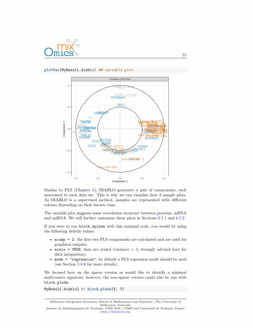
75

plotVar(MyResult.diablo) ## variable plot

NDRG2

ASPM

KDM4B

ZNF552

STAT5A

FUT8

PROM2TANC2

C4orf34

LRIG1

SDC1

STC2CD302

PSIP1

CSRP2

SLC43A3

TTC39A

PLCD3

NTN4

OGFRL1

E2F1CCNA2NCAPG2

PLEKHA4

PREX1

CDK18

MEX3A

ZNF37BTRIM45

ELP2AMN1

SEMA3C

TP53INP2

hsa−let−7d

hsa−mir−101−1

hsa−mir−101−2

hsa−mir−106ahsa−mir−106b

hsa−mir−1301hsa−mir−130b

hsa−mir−146ahsa−mir−17

hsa−mir−186

hsa−mir−195

hsa−mir−197

hsa−mir−20a

hsa−mir−30a

hsa−mir−30c−2

hsa−mir−501

hsa−mir−505

hsa−mir−532hsa−mir−590hsa−mir−9−1hsa−mir−9−2

hsa−mir−92a−2hsa−mir−93

AR

ASNSCyclin_B1

Cyclin_E1

EGFR_pY1068

ER−alpha

GATA3

HER2HER2_pY1248

c−Kit


−1.0 −0.5 0.0 0.5 1.0

−1.0

−0.5

0.0

0.5

1.0

Component 1

Com

pone

nt 2

Similar to PLS (Chapter 5), DIABLO generates a pair of components, eachassociated to each data set. This is why we can visualise here 3 sample plots.As DIABLO is a supervised method, samples are represented with differentcolours depending on their known class.

The variable plot suggests some correlation structure between proteins, mRNAand miRNA. We will further customize these plots in Sections 6.7.1 and 6.7.2.

If you were to run block.splsda with this minimal code, you would be usingthe following default values:


• scale = TRUE: data are scaled (variance = 1, strongly advised here fordata integration);

• mode = "regression": by default a PLS regression mode should be used(see Section 5.8.6 for more details) .

We focused here on the sparse version as would like to identify a minimalmulti-omics signature, however, the non-sparse version could also be run withblock.plsda:MyResult.diablo2 <- block.plsda(X, Y)



http://mixomics.org

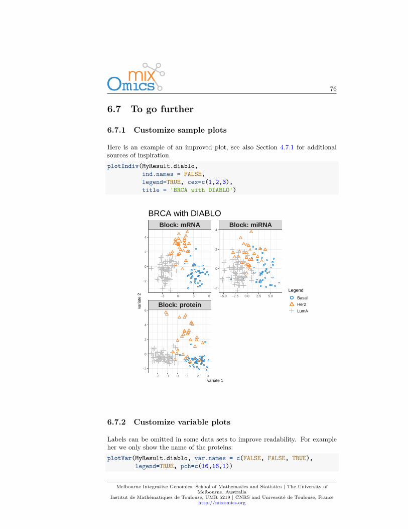
76

6.7 To go further

6.7.1 Customize sample plots

Here is an example of an improved plot, see also Section 4.7.1 for additionalsources of inspiration.plotIndiv(MyResult.diablo,

ind.names = FALSE,legend=TRUE, cex=c(1,2,3),title = 'BRCA with DIABLO')

Block: protein

Block: mRNA Block: miRNA

−2 −1 0 1 2 3

−3 0 3 6 −5.0 −2.5 0.0 2.5 5.0

−2

0

2

4

−2

0

2

4

−2

0

2

4

6

variate 1

varia

te 2

Legend

Basal

Her2

LumA

BRCA with DIABLO

6.7.2 Customize variable plots

Labels can be omitted in some data sets to improve readability. For exampleher we only show the name of the proteins:plotVar(MyResult.diablo, var.names = c(FALSE, FALSE, TRUE),

legend=TRUE, pch=c(16,16,1))



http://mixomics.org

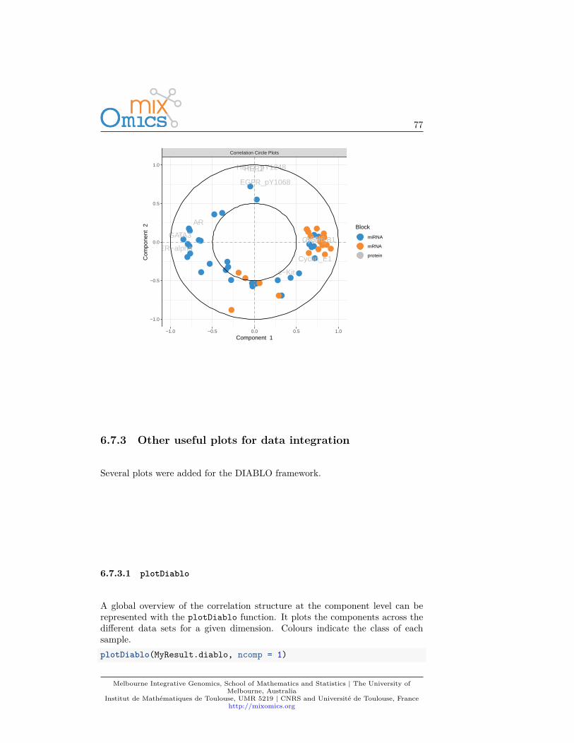
77

AR

ASNSCyclin_B1

Cyclin_E1

EGFR_pY1068

ER−alpha

GATA3

HER2HER2_pY1248

c−Kit


−1.0 −0.5 0.0 0.5 1.0

−1.0

−0.5

0.0

0.5

1.0

Component 1

Com

pone

nt 2 Block

miRNA

mRNA

protein

6.7.3 Other useful plots for data integration

Several plots were added for the DIABLO framework.

6.7.3.1 plotDiablo

A global overview of the correlation structure at the component level can berepresented with the plotDiablo function. It plots the components across thedifferent data sets for a given dimension. Colours indicate the class of eachsample.plotDiablo(MyResult.diablo, ncomp = 1)



http://mixomics.org

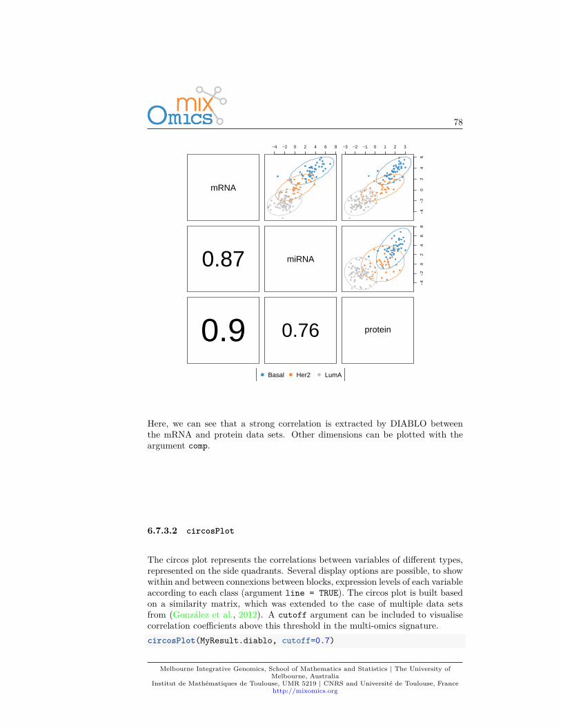
78

Index

mRNA

X.label

Y.la

bel

−4 −2 0 2 4 6 8

X.label

Y.la

bel

−3 −2 −1 0 1 2 3

−4

−2

02

46

Index

0.87

Index

1 miRNA

X.label

Y.la

bel

−4

−2

02

46

8

Index

0.9Index

1 0.76

Index

1 protein

Basal Her2 LumA

Here, we can see that a strong correlation is extracted by DIABLO betweenthe mRNA and protein data sets. Other dimensions can be plotted with theargument comp.

6.7.3.2 circosPlot

The circos plot represents the correlations between variables of different types,represented on the side quadrants. Several display options are possible, to showwithin and between connexions between blocks, expression levels of each variableaccording to each class (argument line = TRUE). The circos plot is built basedon a similarity matrix, which was extended to the case of multiple data setsfrom (González et al., 2012). A cutoff argument can be included to visualisecorrelation coefficients above this threshold in the multi-omics signature.circosPlot(MyResult.diablo, cutoff=0.7)



http://mixomics.org

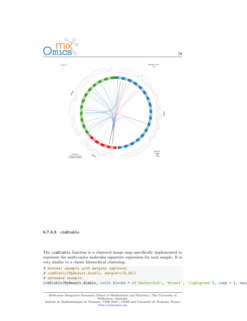
79

C4o

rf34

ZN

F55

2

FU

T8

LRIG

1

TTC

39A

SE

MA

3C

CD

K18

PREX1

KDM4B

TANC2

TRIM45

NTN4

STAT5A

PLEKHA4

STC2

ZNF37B

ELP2

NDRG2

PLCD3

AMN1

CCNA2

PROM2

ASPM

CD302

E2F1

MEX3A

OG

FRL1

SLC43A3

NC

AP

G2P

SIP

1CS

RP

2

TP

53INP

2

SD

C1

mR

NA

AR

GAT

A3

ER

−alp

haAS

NS

Cyc

lin_B

1

HE

R2

Cyc

lin_E

1

c−Kit

HER2_pY

1248

EGFR_pY1068

protein

hsa−mir−30a

hsa−mir−590

hsa−mir−30c−2

hsa−mir−130b

hsa−mir−101−2

hsa−mir−1301

hsa−mir−17

hsa−mir−505

hsa−mir−106b

hsa−mir−501

hsa−mir−101−1

hsa−mir−532

hsa−mir−197

hsa−mir−93

hsa−mir−106a

hsa−mir−186

hsa−mir−146a

hsa−mir−9−2

hsa−mir−20a

hsa−mir−9−1

hsa−let−7d

hsa−mir−195

hsa−m

ir−92a−

2

miR

NA

Correlations

Positive CorrelationNegative Correlation

Expression

BasalHer2LumA

Correlation cut−off

r=0.7Comp 1−2

6.7.3.3 cimDiablo

The cimDiablo function is a clustered image map specifically implemented torepresent the multi-omics molecular signature expression for each sample. It isvery similar to a classic hierarchical clustering:# minimal example with margins improved:# cimDiablo(MyResult.diablo, margin=c(8,20))# extended example:cimDiablo(MyResult.diablo, color.blocks = c('darkorchid', 'brown1', 'lightgreen'), comp = 1, margin=c(8,20), legend.position = "right")



http://mixomics.org

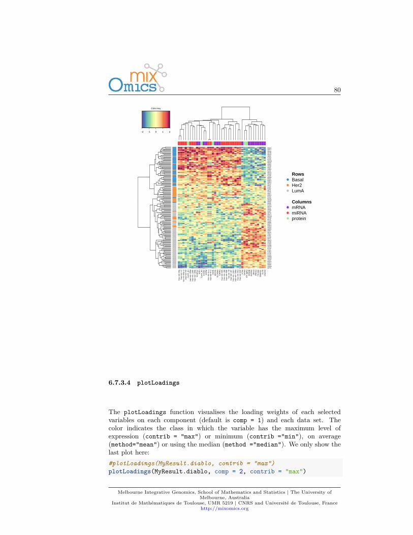
80

−2 −1 0 1 2

Color key

hsa−

mir−

20a

hsa−

mir−

17hs

a−m

ir−92

a−2

hsa−

mir−

93C

yclin

_E1

hsa−

mir−

106a

hsa−

mir−

130b

hsa−

mir−

106b

NC

AP

G2

E2F

1C

yclin

_B1

CC

NA

2A

SP

Mhs

a−m

ir−9−

1hs

a−m

ir−9−

2A

SN

SM

EX

3AS

LC43

A3

CS

RP

2hs

a−m

ir−50

5hs

a−m

ir−18

6hs

a−m

ir−59

0hs

a−le

t−7d

hsa−

mir−

197

hsa−

mir−

1301

hsa−

mir−

146a

hsa−

mir−

501

hsa−

mir−

532

NT

N4

GAT

A3

ER

−al

pha

KD

M4B

ZN

F55

2LR

IG1

PR

EX

1T

TC

39A

SE

MA

3CF

UT

8C

4orf

34

A0T6A0BMA0DPA0EAA0DSA06PA0CSA0BQA12AA146A1B1A1ALA133A0XSA18NA18SA04AA0EUA0YLA15EA15LA0E1A0X0A08TA0RVA0SUA0RHA0H7A0BPA1APA0J5A09GA0XWA0CTA0TZA12TA08AA03LA0XNA12XA086A08XA04WA12PA137A0D1A0A7A094A0T1A152A1ATA0FLA0T2A0RXA0RTA0ALA0DAA13EA0AVA0XUA131A0B9A0ATA0SKA0E0A0G0A0CMA143A1AZA08LA0CEA07RA04UA0FJA0D2

RowsBasalHer2LumA

ColumnsmRNAmiRNAprotein

6.7.3.4 plotLoadings

The plotLoadings function visualises the loading weights of each selectedvariables on each component (default is comp = 1) and each data set. Thecolor indicates the class in which the variable has the maximum level ofexpression (contrib = "max") or minimum (contrib ="min"), on average(method="mean") or using the median (method ="median"). We only show thelast plot here:#plotLoadings(MyResult.diablo, contrib = "max")plotLoadings(MyResult.diablo, comp = 2, contrib = "max")



http://mixomics.org

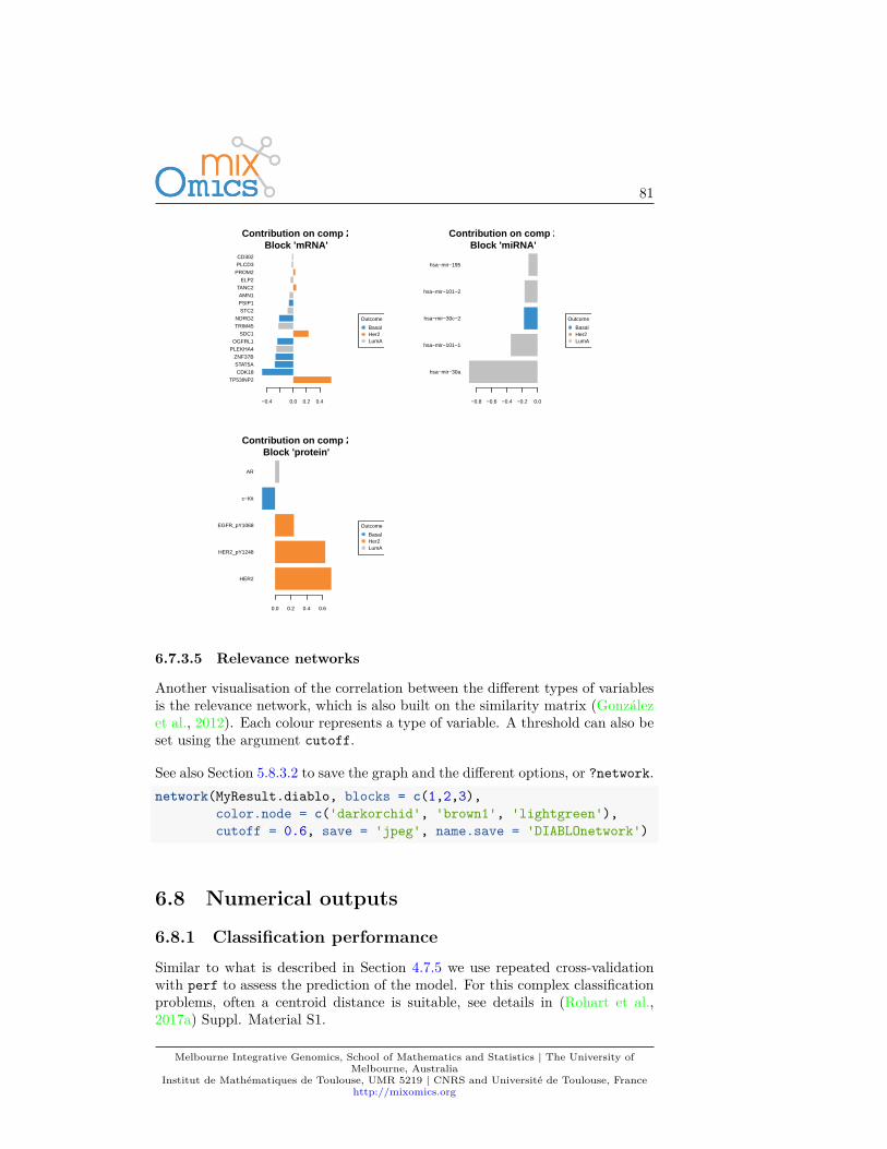
81

TP53INP2

CDK18

STAT5A

ZNF37B

PLEKHA4

OGFRL1

SDC1

TRIM45

NDRG2

STC2

PSIP1

AMN1

TANC2

ELP2

PROM2

PLCD3

CD302

−0.4 0.0 0.2 0.4

Contribution on comp 2Block 'mRNA'

Outcome

BasalHer2LumA

hsa−mir−30a

hsa−mir−101−1

hsa−mir−30c−2

hsa−mir−101−2

hsa−mir−195

−0.8 −0.6 −0.4 −0.2 0.0

Contribution on comp 2Block 'miRNA'

Outcome

BasalHer2LumA

HER2

HER2_pY1248

EGFR_pY1068

c−Kit

AR

0.0 0.2 0.4 0.6

Contribution on comp 2Block 'protein'

Outcome

BasalHer2LumA

6.7.3.5 Relevance networks

Another visualisation of the correlation between the different types of variablesis the relevance network, which is also built on the similarity matrix (Gonzálezet al., 2012). Each colour represents a type of variable. A threshold can also beset using the argument cutoff.

See also Section 5.8.3.2 to save the graph and the different options, or ?network.network(MyResult.diablo, blocks = c(1,2,3),

color.node = c('darkorchid', 'brown1', 'lightgreen'),cutoff = 0.6, save = 'jpeg', name.save = 'DIABLOnetwork')

6.8 Numerical outputs

6.8.1 Classification performanceSimilar to what is described in Section 4.7.5 we use repeated cross-validationwith perf to assess the prediction of the model. For this complex classificationproblems, often a centroid distance is suitable, see details in (Rohart et al.,2017a) Suppl. Material S1.



http://mixomics.org

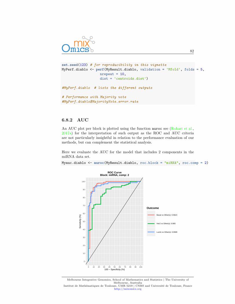
82

set.seed(123) # for reproducibility in this vignetteMyPerf.diablo <- perf(MyResult.diablo, validation = 'Mfold', folds = 5,

nrepeat = 10,dist = 'centroids.dist')

#MyPerf.diablo # lists the different outputs

# Performance with Majority vote#MyPerf.diablo$MajorityVote.error.rate

6.8.2 AUC

An AUC plot per block is plotted using the function auroc see (Rohart et al.,2017a) for the interpretation of such output as the ROC and AUC criteriaare not particularly insightful in relation to the performance evaluation of ourmethods, but can complement the statistical analysis.

Here we evaluate the AUC for the model that includes 2 components in themiRNA data set.Myauc.diablo <- auroc(MyResult.diablo, roc.block = "miRNA", roc.comp = 2)

0

10

20

30

40

50

60

70

80

90

100

0 10 20 30 40 50 60 70 80 90 100100 − Specificity (%)

Sen

sitiv

ity (

%)

Outcome

Basal vs Other(s): 0.9623

Her2 vs Other(s): 0.865

LumA vs Other(s): 0.9589

ROC CurveBlock: miRNA, comp: 2



http://mixomics.org

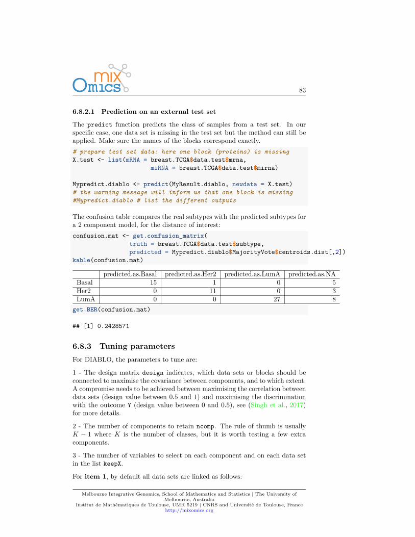
83

6.8.2.1 Prediction on an external test set

The predict function predicts the class of samples from a test set. In ourspecific case, one data set is missing in the test set but the method can still beapplied. Make sure the names of the blocks correspond exactly.# prepare test set data: here one block (proteins) is missingX.test <- list(mRNA = breast.TCGA$data.test$mrna,

miRNA = breast.TCGA$data.test$mirna)

Mypredict.diablo <- predict(MyResult.diablo, newdata = X.test)# the warning message will inform us that one block is missing#Mypredict.diablo # list the different outputs

The confusion table compares the real subtypes with the predicted subtypes fora 2 component model, for the distance of interest:confusion.mat <- get.confusion_matrix(

truth = breast.TCGA$data.test$subtype,predicted = Mypredict.diablo$MajorityVote$centroids.dist[,2])

kable(confusion.mat)

predicted.as.Basal predicted.as.Her2 predicted.as.LumA predicted.as.NABasal 15 1 0 5Her2 0 11 0 3LumA 0 0 27 8

get.BER(confusion.mat)

## [1] 0.2428571

6.8.3 Tuning parametersFor DIABLO, the parameters to tune are:

1 - The design matrix design indicates, which data sets or blocks should beconnected to maximise the covariance between components, and to which extent.A compromise needs to be achieved between maximising the correlation betweendata sets (design value between 0.5 and 1) and maximising the discriminationwith the outcome Y (design value between 0 and 0.5), see (Singh et al., 2017)for more details.

2 - The number of components to retain ncomp. The rule of thumb is usuallyK − 1 where K is the number of classes, but it is worth testing a few extracomponents.

3 - The number of variables to select on each component and on each data setin the list keepX.

For item 1, by default all data sets are linked as follows:



http://mixomics.org

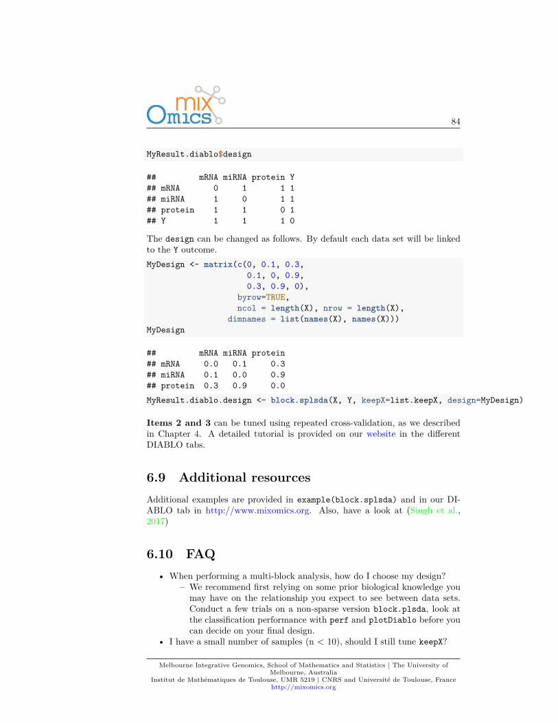
84

MyResult.diablo$design

## mRNA miRNA protein Y## mRNA 0 1 1 1## miRNA 1 0 1 1## protein 1 1 0 1## Y 1 1 1 0

The design can be changed as follows. By default each data set will be linkedto the Y outcome.MyDesign <- matrix(c(0, 0.1, 0.3,

0.1, 0, 0.9,0.3, 0.9, 0),

byrow=TRUE,ncol = length(X), nrow = length(X),

dimnames = list(names(X), names(X)))MyDesign

## mRNA miRNA protein## mRNA 0.0 0.1 0.3## miRNA 0.1 0.0 0.9## protein 0.3 0.9 0.0MyResult.diablo.design <- block.splsda(X, Y, keepX=list.keepX, design=MyDesign)

Items 2 and 3 can be tuned using repeated cross-validation, as we describedin Chapter 4. A detailed tutorial is provided on our website in the differentDIABLO tabs.

6.9 Additional resourcesAdditional examples are provided in example(block.splsda) and in our DI-ABLO tab in http://www.mixomics.org. Also, have a look at (Singh et al.,2017)

6.10 FAQ• When performing a multi-block analysis, how do I choose my design?

– We recommend first relying on some prior biological knowledge youmay have on the relationship you expect to see between data sets.Conduct a few trials on a non-sparse version block.plsda, look atthe classification performance with perf and plotDiablo before youcan decide on your final design.

• I have a small number of samples (n < 10), should I still tune keepX?



http://mixomics.org/mixdiablo/


http://mixomics.org

85

– It is probably not worth it. Try with a few keepX values and lookat the graphical outputs so see if they make sense. With a smalln you can adopt an exploratory approach that does not require aperformance assessment.

• During tune or perf the code broke down (system computationallysingular).

– Check that the M value for your M-fold is not too high comparedto n (you want n/M > 6 − 8 as rule of thumb). Try leave-one-outinstead with validation = 'loo' and make sure ncomp is not toolarge as you are running on empty matrices!

• My tuning step indicated the selection of only 1 miRNA…– Choose a grid of keepX values that starts at a higher value (e.g. 5).

The algorithm found an optimum with only one variable, either be-cause it is highly discriminatory or because the data are noisy, butit does not stop you from trying for more.

• My Y is continuous, what can I do?– You can perform a multi-omics regression with block.spls. We have

not found a way yet to tune the results so you will need to adopt anexploratory approach or back yourself up with downstream analysesonce you have identified a list of highly correlated features.



http://mixomics.org

86



http://mixomics.org

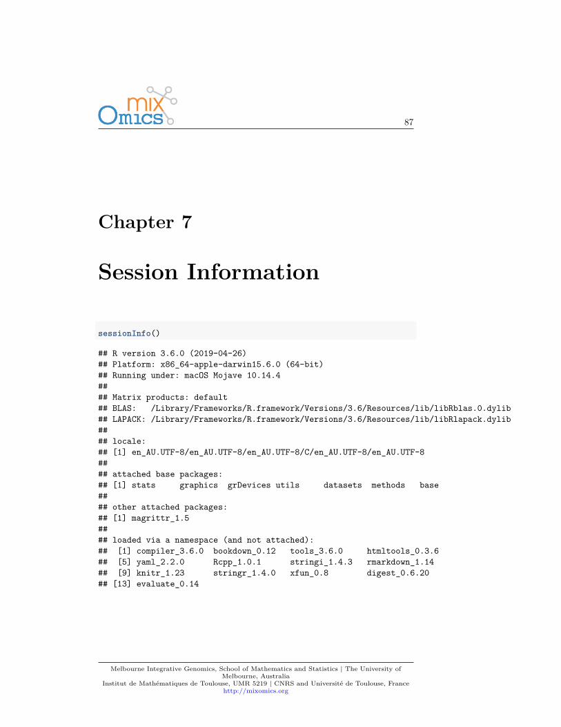
87

Chapter 7

Session Information

sessionInfo()

## R version 3.6.0 (2019-04-26)## Platform: x86_64-apple-darwin15.6.0 (64-bit)## Running under: macOS Mojave 10.14.4#### Matrix products: default## BLAS: /Library/Frameworks/R.framework/Versions/3.6/Resources/lib/libRblas.0.dylib## LAPACK: /Library/Frameworks/R.framework/Versions/3.6/Resources/lib/libRlapack.dylib#### locale:## [1] en_AU.UTF-8/en_AU.UTF-8/en_AU.UTF-8/C/en_AU.UTF-8/en_AU.UTF-8#### attached base packages:## [1] stats graphics grDevices utils datasets methods base#### other attached packages:## [1] magrittr_1.5#### loaded via a namespace (and not attached):## [1] compiler_3.6.0 bookdown_0.12 tools_3.6.0 htmltools_0.3.6## [5] yaml_2.2.0 Rcpp_1.0.1 stringi_1.4.3 rmarkdown_1.14## [9] knitr_1.23 stringr_1.4.0 xfun_0.8 digest_0.6.20## [13] evaluate_0.14



http://mixomics.org

88



http://mixomics.org

89

Bibliography

Barker, M. and Rayens, W. (2003). Partial least squares for discrimination.Journal of chemometrics, 17(3):166–173.

Boulesteix, A. and Strimmer, K. (2005). Predicting transcription factor ac-tivities from combined analysis of microarray and chip data: a partial leastsquares approach. Theor Biol Med Model, 2(23).

Boulesteix, A. and Strimmer, K. (2007). Partial least squares: a versatile tool forthe analysis of high-dimensional genomic data. Briefings in Bioinformatics,8(1):32.

Bylesjö, M., Eriksson, D., Kusano, M., Moritz, T., and Trygg, J. (2007). Dataintegration in plant biology: the o2pls method for combined modeling oftranscript and metabolite data. The Plant Journal, 52:1181–1191.

Cancer Genome Atlas Network et al. (2012). Comprehensive molecular portraitsof human breast tumours. Nature, 490(7418):61–70.

Chung, D. and Keles, S. (2010). Sparse Partial Least Squares Classification forHigh Dimensional Data. Statistical Applications in Genetics and MolecularBiology, 9(1):17.

González, I., Déjean, S., Martin, P. G., and Baccini, A. (2008). CCA: AnR package to extend canonical correlation analysis. Journal of StatisticalSoftware, 23(12):1–14.

González, I., Lê Cao, K.-A., Davis, M. J., Déjean, S., et al. (2012). Visualisingassociations between paired ’omics’ data sets. BioData mining, 5(1):19.

Jolliffe, I. (2005). Principal component analysis. Wiley Online Library.

Khan, J., Wei, J. S., Ringner, M., Saal, L. H., Ladanyi, M., Westermann, F.,Berthold, F., Schwab, M., Antonescu, C. R., Peterson, C., et al. (2001). Clas-sification and diagnostic prediction of cancers using gene expression profilingand artificial neural networks. Nature medicine, 7(6):673–679.



http://mixomics.org

90

Lê Cao, K., Rossouw, D., Robert-Granié, C., Besse, P., et al. (2008). A sparsePLS for variable selection when integrating omics data. Statistical applicationsin genetics and molecular biology, 7:Article–35.

Lê Cao, K.-A., Boitard, S., and Besse, P. (2011). Sparse PLS DiscriminantAnalysis: biologically relevant feature selection and graphical displays formulticlass problems. BMC bioinformatics, 12(1):253.

Lê Cao, K.-A., Costello, M.-E., Chua, X.-Y., Brazeilles, R., and Rondeau, P.(2016). Mixmc: Multivariate insights into microbial communities. PloS one,11(8):e0160169.

Lê Cao, K.-A., Martin, P. G., Robert-Granié, C., and Besse, P. (2009). Sparsecanonical methods for biological data integration: application to a cross-platform study. BMC bioinformatics, 10(1):34.

Mariette, J. and Villa-Vialaneix, N. (2017). Unsupervised multiple kernel learn-ing for heterogeneous data integration. Bioinformatics, 34(6):1009–1015.

Martin, P., Guillou, H., Lasserre, F., Déjean, S., Lan, A., Pascussi, J.-M.,San Cristobal, M., Legrand, P., Besse, P., and Pineau, T. (2007). Novel as-pects of PPARalpha-mediated regulation of lipid and xenobiotic metabolismrevealed through a multrigenomic study. Hepatology, 54:767–777.

Nguyen, D. and Rocke, D. (2002). Tumor classification by partial least squaresusing microarray gene expression data. Bioinformatics, 18(1):39.

Rohart, F., Gautier, B., Singh, A., and Lê Cao, K.-A. (2017a). mixomics: anr package for ‘omics feature selection and multiple data integration. PLoSComputational Biology, 13(11).

Rohart, F., Matigian, N., Eslami, A., S, B., and Lê Cao, K.-A. (2017b). Mint:A multivariate integrative method to identify reproducible molecular signa-tures across independent experiments and platforms. BMC bioinformatics,18(1):128.

Shen, H. and Huang, J. Z. (2008). Sparse principal component analysis viaregularized low rank matrix approximation. Journal of multivariate analysis,99(6):1015–1034.

Singh, A., Gautier, B., Shannon, C., Rohart, F., Vacher, M., S, T., and Lê Cao,K.-A. (2017). Diablo: identifying key molecular drivers from multi-omic as-says, an integrative approach.

Sorlie, T., Perou, C. M., Tibshirani, R., Aas, T., Geisler, S., Johnsen, H., Hastie,T., Eisen, M. B., Van De Rijn, M., Jeffrey, S. S., et al. (2001). Gene expres-sion patterns of breast carcinomas distinguish tumor subclasses with clinicalimplications. Proceedings of the National Academy of Sciences, 98(19):10869–10874.



http://mixomics.org

91

Tan, Y., Shi, L., Tong, W., Gene Hwang, G., and Wang, C. (2004). Multi-classtumor classification by discriminant partial least squares using microarraygene expression data and assessment of classification models. ComputationalBiology and Chemistry, 28(3):235–243.

Tenenhaus, A., Philippe, C., Guillemot, V., Le Cao, K.-A., Grill, J., and Frouin,V. (2014). Variable selection for generalized canonical correlation analysis.Biostatistics, 15(3):569–583.

Tenenhaus, A. and Tenenhaus, M. (2011). Regularized generalized canonicalcorrelation analysis. Psychometrika, 76(2):257–284.

Tenenhaus, M. (1998). La régression PLS: théorie et pratique. Editions Technip.

Teng, M., Love, M. I., Davis, C. A., Djebali, S., Dobin, A., Graveley, B. R., Li,S., Mason, C. E., Olson, S., Pervouchine, D., et al. (2016). A benchmark forrna-seq quantification pipelines. Genome biology, 17(1):74.

Umetri, A. (1996). SIMCA-P for windows, Graphical Software for MultivariateProcess Modeling. Umea, Sweden.

Wold, H. (1966). Estimation of principal components and related models byiterative least squares. New York: Academic Press.

Wold, S., Sjöström, M., and Eriksson, L. (2001). Pls-regression: a basic tool ofchemometrics. Chemometrics and intelligent laboratory systems, 58(2):109–130.



http://mixomics.org

Documents

mixOmics vignette