Embed Size (px)
Citation preview

MKH-Haase Charts of Binocular Vision
Measurements: Repeatability and Validity
of Associated Phoria and Stereotests
by
Mosaad Alhassan
A thesis
presented to the University of Waterloo
in fulfillment of the
thesis requirement for the degree of
Master of Science
in
Vision Science
Waterloo, Ontario, Canada, 2013
© Mosaad Alhassan 2013

ii
AUTHOR'S DECLARATION
I hereby declare that I am the sole author of this thesis. This is a true copy of the thesis, including any
required final revisions, as accepted by my examiners.
I understand that my thesis may be made electronically available to the public.

iii
Abstract
Introduction: H.J.-Haase developed a systematic set of tests for evaluating binocular vision called the
Pola Test. The Pola Test measures associated phoria and stereoacuity at distance and near using a
variety of different targets for each. This testing method and interpretation is referred to as MKH-
Haase (Measuring and Correcting Methodology after H.J.Haase –the MKH) method. The MKH
method is more commonly used in Germany and other European countries than English speaking
countries. The MKH-Haase method has been considered a reliable method for prescribing prisms to
symptomatic binocular vision patients.
Purpose: To investigate the test-retest reliability of binocular vision measurements using the MKH-
Haase series of tests that comprise the Pola Test. In addition, I will compare the Pola results with
other associated phoria and stereoacuity tests used in North America.
Methods: Thirty-four symptomatic and 40 asymptomatic subjects (based on a symptoms
questionnaire) participated in this study. Associated phoria and stereoacuity with different tests,
including the Pola Test at distance and near, were measured for those subjects on two different
sessions. Not all of subjects were tested with all tests. Only 30 subjects in each group completed all of
tests. The Pola Test protocol requires the associated phoria and stereoacuity to be measured twice
within a session; once with the Polariods oriented with their axes at 45o and 135
o and again with the
axes switched.
Results: Within and between-sessions repeatability of MKH-Haase associated phoria and
stereoacuity tests results revealed that most of MKH-Haase associated phoria and stereoacuity tests
showed good repeatability within and between-sessions at both distance and near. However, there
were a few exceptions to this general finding. Distance horizontal associated phoria values for the
Cross Test and Pointer Test at the first session, and the distance Double Pointer Test values at the
second session showed some differences between the two views. Between-sessions repeatability of

iv
the associated phoria tests did not show any significant differences. For the stereoacuity tests, the
differences between the two disparities were statistically significant at the first session for the
symptomatic group Line Test and asymptomatic group Step Test. For the second session at distance,
the differences were significant with Step Test for both groups. The differences between sessions for
both disparities were not significant for most of tests. The symptomatic group’s Step Test for crossed
disparity and asymptomatic group's Step Test for uncrossed disparity were exceptions.
A repeated measures ANOVA test was conducted to compare different associated phoria tests.
Horizontal associated phoria tests without central fusion lock were significantly different from those
with central fusion lock at distance and near. Comparison of different stereoacuity tests was
conducted by comparing the number of subjects who could identify specific stereothreshold values.
Results showed that at both distance and near, there were no significant differences between contour
and global stereoacuity tests based on number of subjects who could attain 60 sec of arc or better.
Discussion and Conclusion: Most of MKH-Haase associated phoria and stereoacuity charts have
reasonable within and between-sessions repeatability. However, some associated phoria tests showed
some differences especially with subjects who had higher values. Although there was a significant
difference between various horizontal associated phoria tests at distance and near, most of the values
differed by around 0.50 . The exception was the difference between the Wesson Card and
Disparometer. The Wesson card was more exo by 1.50 than the Disparometer. Vertical associated
phoria tests did not show any significant differences. Although MKH-Haase chart can measure local
stereothreshold down to 10 sec of arc at distance, the AO Slide is easier to perceive. Random dot
stereoacuity can be measured with MKH-Haase charts at distance down to 30 sec of arc. All of the
contour stereoacuity tests are comparable at near. However, the MKH-Haase chart was easier to
perceive. The Random Dot Randot test would be more useful for fast screening purposes. Random
dot MKH-Haase test would be easier than TNO Test to measure random dot stereothreshold at near.

v
Acknowledgements
I wish to thank my supervisors, Drs. B. Ralph Chou and Jeffery Hovis, who were more than generous
with their expertise and precious time. Special thanks to my MSc advisory committee members, Drs.
Elizabeth Irving and Patrick Quaid, for their guidance and assistance. Their time and effort is highly
appreciated. Special thanks to Dr. Natalie Hutchings for providing the Pola Test. I would like to
acknowledge and thank the School of Optometry and Vision Science, University of Waterloo for
allowing me to conduct my research and providing any assistance requested.
I would like to acknowledge my sponsor, King Saud University in Riyadh, Saudi Arabia and the
Cultural Bureau of Saudi Arabia in Ottawa for supporting me financially during my studies in
Canada.
I would like to acknowledge the Canadian Optometric Educational Trust Fund for the financial
support for this project.

vi
Dedication
I dedicate my thesis work to my family and many friends. A special feeling of gratitude to my loving
parents, my wife, and my brothers and sisters whose words of encouragement provoked me to
accomplish this mission all the way to the last step. I also dedicate this thesis to my many friends who
have supported me throughout the process. I will always appreciate all they have done.

vii
Table of Contents
AUTHOR'S DECLARATION ............................................................................................................... ii
Abstract ................................................................................................................................................. iii
Acknowledgements ................................................................................................................................ v
Dedication ............................................................................................................................................. vi
Table of Contents ................................................................................................................................. vii
List of Figures ....................................................................................................................................... ix
List of Tables ......................................................................................................................................... xi
Chapter 1 General Introduction .............................................................................................................. 1
1.1 Binocular Single Vision and Panum’s Fusional Area .................................................................. 1
1.2 Fixation Disparity, Associated Phoria, and Stereoacuity ............................................................. 3
1.3 Historical Background and Literature Review ............................................................................. 3
1.3.1 Fixation Disparity .................................................................................................................. 3
1.3.2 Stereopsis ............................................................................................................................... 5
1.4 Measurements ............................................................................................................................... 6
1.4.1 Fixation Disparity Curve ....................................................................................................... 6
1.4.2 Stereopsis ............................................................................................................................. 12
1.5 Measuring and Correcting Methodology after H.J. Haase method ............................................ 13
1.5.1 History & Apparatus Development ..................................................................................... 13
1.5.2 Theory ................................................................................................................................. 15
1.5.3 MKH Charts of Binocular Vision ........................................................................................ 16
1.6 Previous Studies ......................................................................................................................... 28
1.6.1 Pola Test .............................................................................................................................. 28
1.6.2 Comparisons of Other Common Associated Phoria and Fixation Disparity Tests .............. 29
1.6.3 Comparisons of Other Common Stereotests ....................................................................... 30
Chapter 2 Purpose ................................................................................................................................ 32
Chapter 3 Apparatus and Charts ........................................................................................................... 34
3.1 MKH charts of Pola Test ............................................................................................................ 34
3.2 Other Associated Phoria Tests at Distance ................................................................................. 34
3.3 Other Associated Phoria and Stereoacuity Tests at Near ........................................................... 35
3.4 Other Stereoacuity Tests............................................................................................................. 38
Chapter 4 Subjects ................................................................................................................................ 41

viii
Chapter 5 Methods ............................................................................................................................... 43
Chapter 6 Results and Discussion ........................................................................................................ 47
6.1 Within session agreement of the MKH-Haase associated phoria charts .................................... 47
6.1.1 Results ................................................................................................................................. 47
6.1.2 Discussion ........................................................................................................................... 62
6.2 Between-session repeatability of the MKH-Haase associated phoria charts ............................. 65
6.2.1 Results ................................................................................................................................. 65
6.2.2 Discussion ........................................................................................................................... 72
6.3 Within session agreement of the MKH-Haase stereoacuity tests .............................................. 75
6.3.1 Results ................................................................................................................................. 75
6.3.2 Discussion ........................................................................................................................... 86
6.4 Between-session repeatability of the MKH-Haase stereoacuity tests ........................................ 88
6.4.1 Results ................................................................................................................................. 88
6.4.2 Discussion ........................................................................................................................... 96
6.5 Within and between-session repeatability of Fixation Disparity Type II according to MKH-
Haase Method (Stereo Triangle and Stereo Balance Tests) ........................................................... 100
6.5.1 Results ............................................................................................................................... 101
6.5.2 Discussion ......................................................................................................................... 105
6.6 Comparison of MKH-Haase associated phoria charts with other common clinical associated
phoria tests ..................................................................................................................................... 107
6.6.1 Results ............................................................................................................................... 108
6.6.2 Discussion ......................................................................................................................... 116
6.7 Comparison of MKH-Haase stereoacuity charts with other common stereoacuity tests ......... 120
6.7.1 Results ............................................................................................................................... 120
6.7.2 Discussion ......................................................................................................................... 128
Chapter 7 Summary and Conclusions ................................................................................................ 131
Copyright Permissions ....................................................................................................................... 135
Bibliography ...................................................................................................................................... 136

ix
List of Figures
Figure 1: Forced Vergence Fixation Disparity Curve ............................................................................ 7
Figure 2: Forced Fixation Disparity Curve Type 1 ................................................................................ 9
Figure 3: Forced Fixation Disparity Curve Type 2 ................................................................................ 9
Figure 4: Forced Fixation Disparity Curve Type 3 .............................................................................. 10
Figure 5: Forced Fixation Disparity Curve Type 4 .............................................................................. 10
Figure 6: Turville’s Infinity Balance Test (TIB) Test .......................................................................... 14
Figure 7: The Pola Test ........................................................................................................................ 15
Figure 8: The Cross Test ...................................................................................................................... 18
Figure 9: The Pointer Test .................................................................................................................... 20
Figure 10: The Double Pointer Test ..................................................................................................... 21
Figure 11: The Rectangle Test ............................................................................................................. 22
Figure 12: The Stereo Triangle Test ..................................................................................................... 24
Figure 13: The Stereo Balance Test ..................................................................................................... 26
Figure 14: The Contour Stereoacuity Test ........................................................................................... 27
Figure 15: Random Dot Stereotests ...................................................................................................... 28
Figure 16: Mallett Test at distance ....................................................................................................... 34
Figure 17: American Optical Vectographic Associated Phoria Slide at distance................................. 35
Figure 18: Mallett Unit at near ............................................................................................................. 36
Figure 19: American Optical Vectographic near point Associated Phoria Test Card .......................... 36
Figure 20: Saladin near point Balance Card ......................................................................................... 37
Figure 21: Sheedy Disparometer .......................................................................................................... 37
Figure 22: Wesson Card ....................................................................................................................... 38
Figure 23: American Optical Vectographic Stereoacuity slide at distance .......................................... 39
Figure 24: Randot Stereotest ................................................................................................................ 39
Figure 25: American Optical Vectographic near point Stereoacuity Card ........................................... 40
Figure 26: TNO Stereotest.................................................................................................................... 40
Figure 27: Horizontal associated phoria of MKH-Haase Cross Test of the 1st session at distance......50
Figure 28: Horizontal associated phoria of MKH-Haase Pointer Test of the 1st session at distance... 51
Figure 29: Vertical associated phoria of MKH-Haase Rectangle Test of the 1st session at distance .. 52
Figure 30: Vertical associated phoria of MKH-Haase Cross Test of the 1st session at near ............... 55

x
Figure 31: Horizontal associated phoria of MKH-Haase Pointer Test of the 2nd session at distance . 58
Figure 32: Horizontal associated phoria of MKH-Haase Double Pointer Test of the 2nd session at
distance ................................................................................................................................................ 59
Figure 33: Between-session repeatability of horizontal associated phoria of MKH-Haase Pointer Test
at distance............................................................................................................................................. 67
Figure 34: : Between-session repeatability of horizontal associated phoria of MKH-Haase Cross Test
at near ................................................................................................................................................... 70
Figure 35: Between-session repeatability of vertical associated phoria of MKH-Haase Rectangle Test
at near ................................................................................................................................................... 71
Figure 36: Within the 1st session agreement of MKH-Haase Line Stereotest at distance ................... 77
Figure 37: Within the 2nd session agreement of MKH-Haase Line Stereotest at distance ................. 81
Figure 38: Within the 2nd session agreement of MKH-Haase Line Stereotest at near........................ 84
Figure 39: Within the 2nd session agreement of MKH-Haase Step Stereotest at near ........................ 85
Figure 40: Between-session repeatability of MKH-Haase Line Test stereothreshold at distance ....... 91
Figure 41: Between-sessions repeatability of MKH-Haase Step Test stereothreshold at distance ...... 92
Figure 42: Comparisons of horizontal associated phoria tests at distance ......................................... 109
Figure 43: Comparisons of horizontal associated phoria tests at distance ......................................... 110
Figure 44: Comparisons of horizontal associated phoria tests at near (Symptomatic Group) ........... 112
Figure 45: Comparisons of horizontal associated phoria tests at near (Asymptomatic Group) ......... 113
Figure 46: Comparisons of vertical associated phoria tests at distance (Symptomatic Group) ......... 115
Figure 47: Comparisons of stereoacuity tests at distance (Symptomatic Group) .............................. 122
Figure 48: Comparisons of stereoacuity tests at distance (Asymptomatic Group) ............................ 123
Figure 49: Comparisons of stereoacuity tests at near (Symptomatic group) ..................................... 126
Figure 50: Comparisons of stereoacuity tests at near (Asymptomatic group) ................................... 127

xi
List of Tables
Table 1: Questionnaire used to classify subjects into symptomatic and asymptomatic ....................... 41
Table 2: Mean difference, 95% CI, and linear regression results of horizontal and vertical MKH-
Haase associated phoria charts at distance (1st Session) ...................................................................... 49
Table 3: Mean difference, 95% CI, and linear regression of horizontal and vertical MKH-Haase
associated phoria charts at near (1st Session) ....................................................................................... 54
Table 4: Mean difference, 95% CI, and linear regression of horizontal and vertical MKH-Haase
associated phoria charts at distance (2nd Session) ............................................................................... 57
Table 5: Mean difference, 95% CI, and linear regression of horizontal and vertical MKH-Haase
associated phoria charts at near (2nd Session) ..................................................................................... 61
Table 6: Mean difference, 95% CI, and linear regression of horizontal and vertical MKH-Haase
associated phoria charts at distance (Between 1st & 2nd Sessions) ..................................................... 66
Table 7: Mean difference, 95% CI, and linear regression of horizontal and vertical MKH-Haase
associated phoria charts at near (Between 1st & 2nd Sessions) ........................................................... 69
Table 8: Between-session repeatability of MKH-Haase associated phoria tests at distance: (Session1
vs. Session2) ......................................................................................................................................... 73
Table 9: Betweensession repeatability of MKH-Haase associated phoria tests at near: (Session1 vs.
Session2) .............................................................................................................................................. 74
Table 10: Mean difference, 95% CI, and linear regression values of the 1st session of MKH-Haase
stereothreshold values at distance (crossed vs. uncrossed disparities) ................................................. 76
Table 11: Within the 1st session repeatability of MKH-Haase Hand Test at distance (crossed vs.
uncrossed) ............................................................................................................................................. 78
Table 12: Mean difference, 95% CI, and linear regression values of the 1st session of MKH-Haase
stereothreshold values at near (crossed vs. uncrossed disparities) ....................................................... 79
Table 13: Mean difference, 95% CI, and linear regression values of the 2nd session of MKH-Haase
stereothreshold values at distance (crossed vs. uncrossed disparities) ................................................. 80
Table 14: Within the 2nd Session repeatability of MKH-Haase Hand test at distance (crossed vs.
uncrossed) ............................................................................................................................................. 82
Table 15: Mean difference, 95% CI, and linear regression values of the 2nd session of MKH-Haase
stereothreshold values at near (crossed vs. uncrossed disparities) ....................................................... 83

xii
Table 16: Mean difference, 95% CI, and linear regression values between-session repeatability of
MKH-Haase crossed disparity stereothreshold values at distance (Crossed Dispari Session 1vs.
Crossed Dispari Session 2) .................................................................................................................. 89
Table 17: Mean Difference, 95% CI, and linear regression values between-session repeatability of
MKH-Haase uncrossed disparity stereothreshold values at distance (Uncrossed Disparity Session 1
vs. Uncrossed Disparity Session 2) ...................................................................................................... 90
Table 18: Between-session repeatability of MKH-Haase Hand test at distance (Session 1 vs. Session
2) .......................................................................................................................................................... 93
Table 19: Mean difference, 95% CI, and linear regression values between-session repeatability of
MKH-Haase crossed disparity stereothreshold values at near (Crossed Disparity Session 1vs. Crossed
Disparity Session 2) ............................................................................................................................. 94
Table 20: Mean difference, 95% CI, and linear regression values between-session repeatability of
MKH-Haase uncrossed disparity stereothreshold values at near (Uncrossed Disparity Session 1 vs.
Uncrossed Disparity Session 2) ........................................................................................................... 95
Table 21: Between-session repeatability of MKH-Haase stereoacuity tests at distance (Session1 vs.
Session2) .............................................................................................................................................. 98
Table 22: Between-session repeatability of MKH-Haase stereoacuity tests at near (Session1 vs.
Session2) .............................................................................................................................................. 99
Table 23: MKH-Haase Stereo Balance tests’ results for the 1st session at distance ......................... 102
Table 24: MKH-Haase Stereo Balance tests’ results for the 1st session at near ................................ 103
Table 25: Frequencies of Subjects who had same results in both sessions of MKH-Haase Stereo
Balance at distance ............................................................................................................................. 104
Table 26: Frequencies of Subjects who had same results in both sessions of MKH-Haase Stereo
Balance at near ................................................................................................................................... 104
Table 27: Horizontal and Vertical Associated Phoria Tests at Distance ............................................ 107
Table 28: Horizontal and Vertical Associated Phoria Tests at Near .................................................. 107
Table 29: 95% limits of agreement for different horizontal associated phoria tests at distance ........ 118
Table 30: 95% limits of agreement for different vertical associated phoria tests at distance ............ 119
Table 31: 95% limits of agreement for different horizontal associated phoria tests at near .............. 119
Table 32: 95% limit of agreement for different vertical associated phoria tests at near .................... 119
Table 33: Stereothreshold for the different stereoacuity tests at distance .......................................... 121
Table 34: Stereothreshold of different stereoacuity tests at near ...................................................... 125

1
Chapter 1
General Introduction
1.1 Binocular Single Vision and Panum’s Fusional Area:
According to the Dictionary of Visual Science, normal binocular single vision can be defined as
“the use of both eyes simultaneously in such a manner that each retinal image contributes to the final
precept” (Hofstetter, 2000).
One of the first attempts to describe binocular single vision was presented by Worth (cited by
Rutstein, 1998; Steinman, 2000; and Rowe, 2004). Worth classified binocular single vision into three
levels or degrees. The first degree was Simultaneous Perception, which is the perception of the two
images of an object of regard from both eyes at the same time. The second degree was Fusion, which
is combining the two images into one image. Fusion was sub-categorized into sensory fusion and
motor fusion. Sensory fusion was the ability of fusing the two images into one. Motor fusion was the
ability to maintain the fused image through a specified range of vergence. The third degree was
Stereoscopic Vision, which was the ability to perceive fine depth from retinal disparities.
Based on the above definition, a person will have normal binocular vision if the image of an
object of regard falls exactly on both foveae and both foveae are assigned the same visual direction.
In this situation, the two foveae are related or corresponding. This correspondence is referred to as
Normal Retinal Correspondence. However, abnormal binocular vision will occur when the fovea of
one eye corresponds with another retinal point of the other eye. This correspondence is referred to as
Abnormal Retinal Correspondence. That is, abnormal retinal correspondence occurs when the fovea
of each eye has different visual directions or the visual direction of the fovea of one eye has the same
visual direction as an extrafoveal point in the other eye (Ogle, 1950; Ogle, 1958; Rutstein, 1998;
Steinman, 2000; and Rowe, 2004).

2
Panum in 1858 (cited by Carter, 1957) proposed that the fovea of one eye could correspond to an
area surrounding the fovea of the other eye. This area was called Panum’s Fusional Area (PFA). This
kind of correspondence was called Point to Area Correspondence and binocular single vision was
still maintained in this situation even though there was a deviation in the visual direction of one eye
(Carter, 1957; Mitchell, 1966b). Howard (2002) reported that the concept of corresponding points
between the two eyes and the fusional area was proposed before Panum. According to Howard, the
first known person who described the correspondence between the two eyes was Alhazan ibn
Alhaytham. Alhazan was a scholar who lived in the 11th century in Iraq then Egypt. Alhazan
described this phenomenon in his book Kitab Al-Manazer (The Book of Optics). Alhazan realized that
binocular single vision still occurred even though there were small differences in the visual angles
between the two eyes. He also noted that diplopia occurred if the differences in the visual angles
exceeded a certain limit (Howard, 2002).
All points in the space that fall on corresponding points in each eye are located on an imaginary
surface called the Horopter (Howard, 2008). Hence, any object located on the horopter produces a
single image. However, if an object lies in front of, behind, above, or below the horopter, a horizontal
or vertical retinal disparity is generated. If the disparity is not too large, then the objects will appear
single and a horizontal disparity will appear in depth (Howard, 2008; Harris and Jenkin 2011;
Stidwill, 2011). This space around the horopter is called Panum’s Fusional Space (Mallettt, 1974).
The two dimensional projection of this space is called Panum’s fusional area (Nelson, 1988). If the
image of the object falls outside Panum’s space, the object is perceived as a double image, yet depth
perception is still possible (Howard, 2008). Mitchell (1966a, 1966b) described Panum’s area as an
oval shape with more horizontal extension than vertical. The horizontal dimension varies between 1
and 20 min of arc (Ames & Ogle, 1932; Palmer, 1961) depending on retinal eccentricity (Weymouth,
1958), duration of stimulus, size of stimulus, and vergence adaptation (Schor, 1980).

3
1.2 Fixation Disparity, Associated Phoria, and Stereoacuity:
Fixation disparity is the small ocular misalignment of one eye or both eyes when the two eyes
are fixating on an object during normal binocular vision. The two images in the case of fixation
disparity do not stimulate normal retinal correspondence, but they fall within Panum’s fusional area;
thus, single binocular vision is perceived (Ogle, Mussey& Prangen, 1949; Ogle, 1950; and Ogle,
1958). If nonius lines are presented dichoptically, while the person fuses an object, the nonius lines
will not be perceived in the same visual direction when a fixation disparity is present. Schor (1980)
described fixation disparity as a small error in the vergence system that is required to maintain fusion
when the fast component of the vergence system changes. To reduce a fixation disparity to zero,
horizontal or vertical prisms are used. The smallest amount of prism to reduce fixation disparity to
zero is called the associated phoria (Brownlee & Goss, 1988; Hofstetter, 2000; Scheiman, 2008).
Stereoacuity or stereopsis is the ability to perceive depth when looking at a scene with both eyes
(Ogle, 1950). Because we have two eyes separated horizontally in the head, each eye will receive a
slightly different image than the other. This separation between the two images is called retinal
disparity. When the two images are combined, a 3-D image is perceived (Howard, 2008).
Stereoacuity assessment is a general test of binocular vision. Individuals with good ocular alignment
and sensory fusion will be able to achieve a stereoacuity of 60 seconds of arc or better. Higher
stereoacuity values may indicate suppression of one eye due to ocular misalignment (Rutstein, 1998).
1.3 Historical Background and Literature Review:
1.3.1 Fixation Disparity:
Wheatstone carried out one of the earliest attempts to understand the fixation disparity
phenomenon (Ogle, 1950). He presented two similar images to both eyes using a haploscope. He
noticed that fusion was still possible even though there were unequal image sizes between the two

4
eyes. This finding led Panum in 1858 to assume that there was a small area around the fovea where
fusion could be maintained. This assumption was made as an explanation for perceiving a single
image of two haploscopically vertical lines even though there is a small difference in angular
separation (15 to 20 min of arc) between them.
The next century involved further observation and measurement (Carter, 1957; Howard, 2002);
however, fixation disparity was usually referred as fixation lag or retinal slip. Lau (cited by Carter
1957) was one of the first to measure systematically the extent of the fixation disparity. He used a
haploscope to present a binocularly viewed central target and nonius lines were presented
dichoptically in the peripheral field. The arms were moved so that the peripheral lines were aligned.
Ogle and his coworkers were the first to use the term Fixation Disparity (Ogle et al., 1949; Ogle &
Prangen, 1951; Ogle & Prangen, 1953).They proposed that the fixation disparity was due to a
muscular imbalance of the two eyes. This imbalance could be increased by placing prisms or lenses of
varying powers in front of the eyes while the observer looked at two polarized nonius dichoptic lines.
The angular separation between the two lines was the amount of fixation disparity. The fixation
disparity plotted as a function of different power of prisms or lenses was known as the forced
vergence fixation disparity curve (FDC). The curve was then analyzed in order to reach the
appropriate management options for individuals with nonstrabismic binocular vision problems. This
method of measuring fixation disparity is widely accepted and followed by all available clinical tests
of fixation disparity.
Another method of assessing fixation disparity was proposed by Remole (1983, 1984, 1985), and
Remole, Code, & Matyas (1986). Remole measured the small deviation from the central fixation by
measuring the width of a vertical border enhancement band. He found that as the retinal eccentricity
increased the width of the enhancement band increased. The increase in the bandwidth can be
converted to an equivalent amount of angular separation to measure the fixation disparity.

5
H.J. Haase (cited by Schroth, 2012) developed a theory as to how the fixation disparity could lead
to binocular vision problems and eventually strabismus. He claimed that untreated fixation disparity
would stress the vergence system. If the vergence demand has increased, the binocular visual system
will be stressed and the fusional vergence will not be able to compensate the new vergence demand.
As a result, a small deviation in one eye will develop. The Panum’s fusional area of the deviated eye
will be stressed to compensate the small error in the vergence system. As a result, PFA in the deviated
eye would enlarge to compensate this stress, which would increase the amount of the deviation
toward a certain direction. Further binocular vision deterioration may develop such as low
stereoacuity and or suppression according to Haase.
1.3.2 Stereopsis:
In 1919, Howard introduced the Howard-Dolman apparatus. It is considered to be one of the oldest
methods to assess stereoacuity. It was used mainly to test the stereoacuity of US army pilots. This test
has been used widely in clinical assessments and research (Howard, 1919; Larson, 1985; Eskridge,
1991).Verhoeff (1942) introduced a portable test to assess the stereoacuity at near. The test was
composed of a central rectangle with three vertical strips inside it. The strips were presented in real
depth, and the patient had to decide which strip appeared closer and which one appeared farther away.
Polaroid vectographic cards were introduced by Wirt in 1947. The polarized cards contained a series
of circles surrounded by squares. One eye saw the circles and the other eye saw the squares. The
patient was asked if he or she could see a figure in depth. The disparity between the two images was
decreased from the top of the card to the bottom.
Stereoacuity can be assessed by generating a pattern with random dots, lines, or shapes. This
method was introduced by Julesz (1960). There are no monocular clues or contours present in the
patterns. Any forms or shapes are visible only if stereopsis is present.
6
1.4 Measurements:
1.4.1 Fixation Disparity Curve:
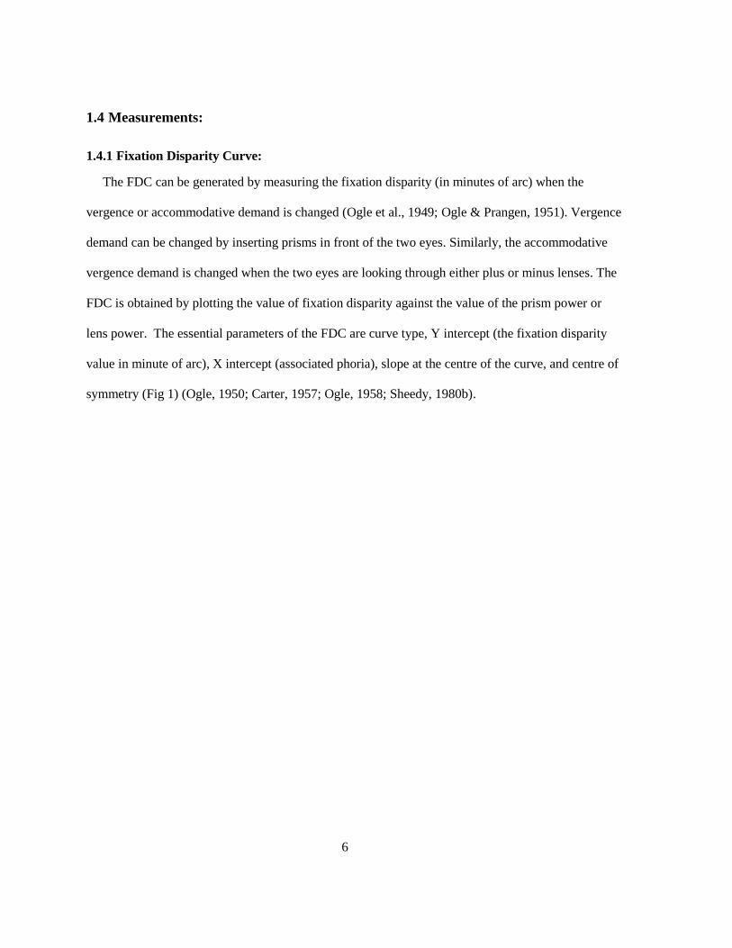
The FDC can be generated by measuring the fixation disparity (in minutes of arc) when the
vergence or accommodative demand is changed (Ogle et al., 1949; Ogle & Prangen, 1951). Vergence
demand can be changed by inserting prisms in front of the two eyes. Similarly, the accommodative
vergence demand is changed when the two eyes are looking through either plus or minus lenses. The
FDC is obtained by plotting the value of fixation disparity against the value of the prism power or
lens power. The essential parameters of the FDC are curve type, Y intercept (the fixation disparity
value in minute of arc), X intercept (associated phoria), slope at the centre of the curve, and centre of
symmetry (Fig 1) (Ogle, 1950; Carter, 1957; Ogle, 1958; Sheedy, 1980b).

7
Figure 1: Forced Vergence Fixation Disparity Curve

8
1.4.1.1 Curve Type:
Curve type is considered to be the most important feature among the FDC parameters to
discriminate symptomatic patients from asymptomatic patients and to determine further steps in the
therapy strategy (Sheedy & Saladin, 1978). According to Ogle, there are four types of fixation
disparity curves. They are Type I, II, III, and IV (Fig. 2-5). Individuals who show a Type I curve are
characterized by an equal adaptation to both base-in and base-out prism. The Type I curve is usually
present with asymptomatic individuals. However, other curve types indicate an abnormality in the
binocular vision status. Type II curve individuals show more adaptation to base-out prism and less
adaptation to base-in prism. Patients with Type II curve usually have an eso-deviation. Type III curve
patients adapt to base-in prism more than base-out prism and they usually have an exo-deviation.
Type IV curve indicates unstable binocular vision and bad vergence adaptation (Palmer & Von
Noorden, 1978; Schor, 1979a&b; Yekta & Pickwell, 1986).Variability in vergence adaptation is the
main reason behind the four FDC types (Schor, 1979 a&b). Schor stated that flat fixation disparity
curves occur when vergence adaptation is high.

9
Figure 2: Forced Fixation Disparity Curve Type 1
Figure 3: Forced Fixation Disparity Curve Type 2

10
Figure 4: Forced Fixation Disparity Curve Type 3
Figure 5: Forced Fixation Disparity Curve Type 4

11
1.4.1.2 Centre of Symmetry:
Centre of symmetry is the most flat area in the forced vergence fixation disparity curve, which is
characterized by the susceptibility of the vergence adaptation to change its behavior within the
fusional vergence (Fig. 1) (Rutstein, 1998; Scheiman, 2008).
1.4.1.3 Y- Intercept (Fixation Disparity Value):
The Y intercept represents the fixation disparity value in the graph when there are no prisms or
lenses in front of the eyes. It is measured in minutes of arc. According to Schor, the magnitude of the
fixation disparity can increase markedly if there is a decline in the sensory fusion function such as a
foveal suppression (Schor, 1979a; Schor, 1979b). Foveal suppression causes the Panum’s fusional
area to extend its size to allow for binocular fusion. This leads to a higher fixation disparity in order
to avoid diplopia. Fixation disparity can be measured clinically by different devices. The most
common ones are the Wesson Card, Sheedy Disparometer, and Saladin Card. The clinical procedures
of those tests are not discussed in this thesis. Full clinical descriptions for those tests can be found in
other literature (Eskridge, 1991; Rutstein, 1998; Scheiman, 2008).
1.4.1.4 X-Intercept (Associated Phoria):
The X intercept is the fourth parameter of the forced vergence fixation disparity curve. It is also
called the associated phoria. It is defined as the amount of prism required to reduce the fixation
disparity to zero. It has been confused by clinicians as the fixation disparity value. It was thought by
Mallettt that the associated phoria is a dependable criterion to assess the lateral fixation disparity. In
contrast, Sheedy and Saladin studied the importance of all of the FDC parameters and they concluded
that the associated phoria value is the least important factor in order to classify the individuals as
symptomatic or asymptomatic (Sheedy & Saladin, 1977; Sheedy, 1980a). Mallett also suggested the
associated phoria is a useful indicator to determine the prescription for symptomatic individuals
(Mallettt, 1974). Indeed, the associated phoria value has been recommended as a good indicator for

12
prescribing vertical prisms (London & Wick, 1987). Associated phoria can be measured clinically
without generating a fixation disparity curve. The most common instruments to measure the
associated phoria at distance are Mallett Test and the American Optical Vectographic Slide. At near,
there are Mallett Unit and Near Point American Optical Vectographic Card. These instruments are
detailed in other sources (Eskridge, 1991; Rutstein, 1998; Scheiman, 2008).
1.4.1.5 Slope:
The last parameter of the FDC is the slope. The slope can be determined by measuring the
difference in the fixation disparity values between 3-prism dioptres base-in and 3-prism dioptres base-
out. Schor considered this as the best symptoms indicator among other FDC parameters (Schor,
1979a; Schor, 1979b). An individual who has a flat slope usually has a good vergence adaptation. On
the other hand, a steep slope is an indicator for a bad vergence adaptation, which is usually flattened
by vision therapy (Sheedy & Saladin, 1978). The slope can be used as guide for prescribing for
symptomatic patients. For those who have a flat fixation disparity curve, the main goal is to try to
shift the center of symmetry toward the Y-axis by either prisms or lenses. This reduces the symptoms
and improves the binocularity (Schor, 1979a; Schor, 1979b).
1.4.2 Stereopsis:
Stereopsis can be tested in clinic by various instruments. All of them are designed in such a way
that each eye looks at two similar targets from slightly different viewing angles. One of the targets is
located exactly on the horopter; however, the other one is off the horopter, which creates retinal
disparity. As the person combines the two targets into one percept, a single target is perceived in
depth. As the distance between the two targets becomes greater, the impression of depth from the
reference plane increases. A person with good stereoacuity would have a small threshold angle of
disparity and vice versa (Howard, 2008).
13
Clinically, stereoacuity tests are classified into three main categories. The first category is the real
stereotest. This kind of stereotest uses real moveable objects to measure the stereoacuity. The most
famous example of this category is the Howard- Dolman Stereotest. The second category is contour
or local stereotests. Stereoacuity in this category is assessed with simple shapes, such as circles, lines,
or any known objects like animals. Examples of the contour based tests are the Titmus Fly Test, AO
Slide, and Randot circles. The third category is random dot or global stereotests. This kind of stereo
testing uses a random dot pattern to generate a shape through the impression of depth (Julesz, 1960).
Examples of the global based tests are the Frisby Test, TNO Test, Randot stereotests, and Random
Dot E test. More details about those instruments can be found in other literature (Eskridge, 1991;
Rutstein, 1998; Scheiman, 2008).
1.5 Measuring and Correcting Methodology after H.J. Haase method:
This testing method and interpretation of fixation disparity was first proposed by H.J Haase in
1956. The series of tests was referred to as the Pola Test. Pola Test measures associated phoria and
stereoacuity at distance and near using a variety of different targets for each. The interpretation of the
results was referred to as Measuring and Correcting Methodology after H.J. Haase (MKH-Haase
method). This series of tests and interpretation is frequently used in Germany (Kommerell, Gerling,
Ball, De Paz, & Bach, 2000; Gerling, De Paz, Schroth, Bach, & Kommerell, 2000; Brautaset &
Jennings, 2001; R. London & Crelier, 2006).
1.5.1 History & Apparatus Development:
The main principle of the Pola Test is based on Turville’s Infinity Balance Test (TIB method) (Fig
6). The TIB test was first presented by Albert Edward Turville in 1937 in Germany.

14
Figure 6: Turville’s Infinity Balance Test (TIB) Test (After, London, R. 2006)
TIB test was designed to measure binocular vision functions. The test consisted of five subtests.
They were horizontal associated phoria, vertical associated phoria, rotational phoria, aniseikonia, and
stereopsis. The major difference between the TIB and the Pola Test is that the TIB used a septum to
present dichoptic stimuli, whereas the Pola Test uses polarized objects for dichoptic presentation. In
addition to the dichoptic targets, there are either peripheral or central fusion locks, which are not
polarized. Fig 7 shows two examples of the Pola Test distance associated phoria targets.
Order Detail ID: 63834388
Strabismus by TAYLOR & FRANCIS THE NETHERLANDS. Reproduced with permission of
TAYLOR & FRANCIS THE NETHERLANDS in the format republish in a thesis/dissertation
via Copyright Clearance Center.

15
Figure 7: The Pola Test
1.5.2 Theory:
Prescribing prism based on the Pola Test is based on the Haase’s theory of binocular vision. He
classified the individuals into three categories based on their vergence adaptation to fixation disparity
and small deviation. The first category is characterized by having enough fusional vergence to
compensate the vergence demand. He called this type of small deviation a Motor Fully Compensated
Heterophoria. In this case, the phoria is fully compensated and the heterophoric persons are usually
asymptomatic.
If the vergence demand is increased, the binocular visual system will be stressed and the fusional
vergence will not be able to compensate the new vergence demand. As a result, a small deviation in
one eye will develop. The Panum’s fusional area of the deviated eye will be stressed to compensate
the small error in the vergence system. According to Haase, this is the first degree of fixation
disparity and he initially called it Disparate Fusion. Later, he gave it another name, Fixation
Disparity Type I. In this type of fixation disparity, the PFA is stressed nasally in eso-deviation,

16
temporally in exo-deviations, and vertically in the hyper or hypo-deviations. At this stage of fixation
disparity, patients may complain from asthenopia and eye fatigue. Stereopsis function may be
affected as well. If fixation disparity Type I is left untreated over time, the stress on the border of PFA
will increase and PFA will enlarge to compensate the strong vergence demand. As a result, an
abnormal retinal correspondence will develop between pseudofoveal points (within PFA) in the
deviated eye and the fovea in the fixing eye. This is the second step of sensory adaptation and it was
referred as Disparate Correspondence or Fixation Disparity Type II by Haase. The connection
between the new corresponding points will be firmer with time if the fixation disparity is left
untreated. In the later stage, a foveal scotoma may develop which will affect the visual acuity of the
deviated eye. Severe stereopsis deterioration and eccentric fixation may be noticed as well (Schroth,
2012).
1.5.3 MKH Charts of Binocular Vision:
Haase divides the heterophoria into two parts; motor and sensory. The motor compensated part of
the heterophoria, which is the muscular adaptation to heterophoria, can be measured by the Cross
Test. This test is administered first. The sensory adaptation tests are presented next in the following
order, the Pointer Test, the Double Pointer Test, Rectangle Test, Stereo Triangle Test, Stereo-Balance
Test, and Stereoacuity Tests. The patient must wear the full optical correction for the refractive error
if there is any. The fixation disparity and small deviations can be measured at both distance and near
with the Pola Test (Gerling, Ball, Bömer, Bach, & Kommerell, 1998; Schroth, 2012).The next section
will describe each test of the Pola Test series and then outline how the sequence is used to determine
the appropriate therapy.

17
1.5.3.1 The Cross Test:
Figure 8 shows the Cross Test. With Polaroid filters in front of the two eyes, the right eye sees the
vertical lines and the left eye can see the horizontal lines. The presentation to each eye can be
switched by twirling the Polaroid filters around the horizontal axes. In this presentation, the right eye
sees the horizontal lines and the left eye sees the vertical lines. Only peripheral fusions locks are
present (the edge of the screen). The main principle of this test is to measure the vertical and
horizontal associated phorias. The Cross Test is used to measure the motor component of the
heterophoria. If the two lines are intersecting exactly at the centre, Haase called this adaptation a
motor fully compensated heterophoria. However, if there is misalignment between the two lines,
prisms are added to realign the vertical and horizontal lines. When the final prism is determined in the
Cross Test, the next step is to examine the patient with the Pointer Test.

18
Figure 8: The Cross Test
The frame is seen by both eyes. The vertical line is seen by one eye. The horizontal line is
seen by the other eye. (After, Brautaset, R.L. 2001)
Order Detail ID: 63834388
Strabismus by TAYLOR & FRANCIS THE NETHERLANDS. Reproduced with permission of
TAYLOR & FRANCIS THE NETHERLANDS in the format republish in a thesis/dissertation
via Copyright Clearance Center.

19
1.5.3.2 The Pointer Test:
Figure 9 shows a diagram of the test. The central black circle serves as a central fusion lock along
with the peripheral locks of the edges. The needle is seen by one eye and the reticules at the top and
bottom are seen by the other eye. This test was designed to measure the cyclophoria along with any
associated horizontal phoria.
Haase described any deviation of the Pointer from the centre of the peripheral scales as the fixation
disparity type I or disparate fusion. This deviation results from a tiny enlargement in the Panum’s
fusional area. The amount of horizontal prism that redirects the two pointers toward the centres of the
two scales is added above the prisms that were determined by the Cross Test previously. If the two
pointers are curved, it is an indication that the patient has the fixation disparity type II or disparate
correspondence. After determining the correct amount of prism, the clinician proceeds to the next test,
which is the Double Pointer Test.

20
Figure 9: The Pointer Test
The Central circle and the surrounding black frame are seen by both eyes. The 2 pointers are
seen by one eye. The 2 scales marks are seen by the other eye. (After, Brautaset, R.L. 2001)
Order Detail ID: 63834388
Strabismus by TAYLOR & FRANCIS THE NETHERLANDS. Reproduced with permission of
TAYLOR & FRANCIS THE NETHERLANDS in the format republish in a thesis/dissertation
via Copyright Clearance Center.

21
1.5.3.3 The Double Pointer Test:
Figure 10 shows the Double Pointer Test. The addition of the horizontal pointer and scales are used
to determine whether there is disparate fusion resulting from a vertical phoria. Vertical prisms are
added if needed.
Figure 10: The Double Pointer Test
The Central circle and the surrounding black frame are seen by both eyes. The 4 pointers are
seen by one eye. The 4 scale marks are seen by the other eye. (After Brautaset, R.L. 2001)
Order Detail ID: 63834388
Strabismus by TAYLOR & FRANCIS THE NETHERLANDS. Reproduced with permission of
TAYLOR & FRANCIS THE NETHERLANDS in the format republish in a thesis/dissertation
via Copyright Clearance Center.

22
1.5.3.4 The Rectangle Test:
Figure 11 shows the Rectangle Test, which is the fourth test in the sequence. The Rectangle test is
also called the E-test. This test was originally used to measure the aniseikonia and any additional
vertical associated phoria. The central circle and edges of the display are the fusion locks. Each side
of the inner rectangle can be seen by one eye. Vertical prisms are added or modified if needed.
Figure 11: The Rectangle Test
The Central circle and the surrounding black frame are seen by both eyes. The right half of
the square is seen by one eye. The left half is seen by the other eye. (After, Brautaset, R.L. 2001)
Order Detail ID: 63834388
Strabismus by TAYLOR & FRANCIS THE NETHERLANDS. Reproduced with permission of
TAYLOR & FRANCIS THE NETHERLANDS in the format republish in a thesis/dissertation
via Copyright Clearance Center.

23
1.5.3.5 The Stereo Triangle Test:
Figure 12 shows the Stereo Triangle Test which is designed to measure Haase fixation disparity
type II. The test chart has both central and peripheral fusion locks. There are two polarized triangles
above and below the central circle. In the standard polarization setting, the right eye sees the left
triangles and the left eye sees the right triangles. This polarization is called contralateral polarization
or (heteronymous polarization) and is synonymous with a crossed retinal disparity. If stereopsis is
present, then the triangles appear to be in front of the circle. If the Polaroid axes are switched then the
triangles are perceived as behind. This later polarization is called ipsilateral polarization or
(homonymous polarization).
For this test, the examiner shows the patient each type of disparity, starting with the crossed
disparity. The time taken by the patient to identify the correct direction in depth of the triangles is
monitored. If the patient can quickly and successfully determine the correct position of the triangles
with both presentations, the fixation disparity is fully compensated. On the other hand, if there is a
delay in perceiving one of the directions in depth, then the patient has a fixation disparity Type II.
Uncorrected or under corrected esophoric patients may have a delay in perceiving the uncrossed
disparity and exophoric patients may have difficulty with the crossed disparity. If there is a delay in
one direction, prism is introduced to equalize the time required to perceive each disparity.

24
Figure 12: The Stereo Triangle Test
The central circle and the border frame are seen binocularly. The right sees the left triangles and the
left eye sees the right triangles (cross disparity). The right eye sees the right triangles and the left eye
sees the left triangles (uncrossed disparity) (After Brautaset, R.L. 2001)
Order Detail ID: 63834388
Strabismus by TAYLOR & FRANCIS THE NETHERLANDS. Reproduced with permission of
TAYLOR & FRANCIS THE NETHERLANDS in the format republish in a thesis/dissertation
via Copyright Clearance Center.

25
1.5.3.6 The Stereo Balance Test:
The Stereo Balance Test is also called a Stereo Valence Test. It can be used also as the previous
one to assess the long-standing retinal correspondence fixation disparity type II. Figure 13 shows that
the display is nearly identical to the stereotest. The difference is the addition of the scales above and
below the central circle. The Stereo Balance Test describes the ocular dominance of one eye in terms
of the perceived visual direction when the two eyes are looking to a stereoscopic image. If the top and
the bottom triangles, are pointing exactly at the centre of the scale marks, there is no ocular
dominance and it is called Isovalence. However, Anisovalence is the term used when one, or both,
triangles are deviated from the centre of the scale. An anisovalence indicates that there is an ocular
dominance of one eye. An Anisovalence suggests that there is a long-standing fixation disparity,
retinal suppression, low visual acuity in one eye, or incorrect optical prescription. For example, in the
uncrossed disparity presentation, the right eye sees the right triangles and the left eye sees the left
triangles. If the fused triangles are shifted toward the right of the scale, then there is a right eye ocular
dominance, which suggests that there could be a problem with the left eye. Furthermore, it indicates
that there is a left eye eso fixation disparity (Schroth, 2012).To reduce the Anisovalence, prisms are
inserted or modified in front of the eyes in discrete steps until Isovalence is obtained for both crossed
and uncrossed disparities.

26
Figure 13: The Stereo Balance Test
The central circle and the border frame are seen binocularly. The right sees the left triangles and the
left eye sees the right triangles (cross disparity). The right eye sees the right triangles and the left eye
sees the left triangles (uncrossed disparity) (After Brautaset, R.L. 2001)
1.5.3.7 The Stereoacuity Tests:
There are several stereotest charts in the Pola test depending upon the version. Figure 14 shows an
example of local stereoacuity chart of the Pola test (version 1.2) used in this study. One test measures
local stereopsis using simple vertical lines. There are 8 different disparities available with this test.
Order Detail ID: 63834388
Strabismus by TAYLOR & FRANCIS THE NETHERLANDS. Reproduced with permission of
TAYLOR & FRANCIS THE NETHERLANDS in the format republish in a thesis/dissertation
via Copyright Clearance Center.

27
The largest disparity is 300 sec of arc, and the disparities decrease to 10 arc sec. There are also two
random dot stereotests for measuring global stereopsis. One is the Random Dot Step Test and the
other is the Random Dot Hand Test. The Random Dot Hand is only presented at distance and the
hand form is a single unknown disparity. The Hand test is scored as pass/fail. The steps test presents 5
rectangles in different disparities of 360, 180, 90, 60, and 30 second of arc, and one circle of unknown
disparity for us (Fig 15).
Figure 14: The Contour Stereoacuity Test

28
A) Step Test
B) Hand Test
Figure 15: Random Dot Stereotests
(The shapes in gray represent the perceived shape in depth in a random dot pattern)
1.6 Previous Studies:
1.6.1 Pola Test:
To my knowledge, only two studies exist in the English literature, which have evaluated the Pola
Test- MKH method (Lie & Opheim, 1985; Lie & Opheim, 1990). In the first study, Lie used the
MKH full correction method for prescribing relieving prisms for 46 symptomatic patients. Most of his

29
patients required several increments in the prism power before stabilizing. The subjects were
evaluated 1 year after constant wear of the full prismatic correction. In the second study, Lie used the
same correcting method for prescribing relieving prisms for 20 heterophoric and 10 heterotropic
patients. The subjects in this study were evaluated 1 year and 5 years after constant wear of the full
prismatic correction. Most of the subjects’ symptoms were relieved and the visual functions were
improved. In the other study, Haase determined the correcting prism from the MKH Cross Test and
compared it with Maddox Rod measurements. The prismatic power determined from the Cross Test
was lower and more comfortable for all of his heterophoric patients in comparison with Maddox Rod
measurements (Haase, 1962). To my knowledge, there have been no direct comparisons between
MKH-Haase charts and other associated phoria or stereotests charts or any evaluation of the
reliability of the MKH-Haase charts.
1.6.2 Comparisons of Other Common Associated Phoria and Fixation Disparity Tests:
A few studies have compared the associated phoria measured on various tests used primarily in
North America. Brownlee and Goss (1988) reported that the distance Mallett Unit and AO
Vectographic Slide associated phorias were not statistically significantly different. At near, the AO
cards and Bernell lantern results were statistically identical; however, the associated phoria measured
on both tests was significantly lower in magnitude than the value measured with the Sheedy
Disparometer.
Two other studies compared the Wesson Card and the Sheedy Disparometer measurements of
associated phorias (Van Haeringen, McClurg, & Cameron, 1986; Goss & Patel, 1995). The findings
were that the Wesson card values were significantly more in the exo direction (base in) compared
with the Disparometer. The differences in the findings between the two tests are likely to be due to
the differences in their designs. Ngan, Goss & Despirito (2005) compared the fixation disparity curve

30
parameters obtained with Wesson and Saladin Cards. The X-Intercept values of Wesson Card tended
to be more exo compared with the Saladin Card. The fixation disparity measured with the Wesson
Card was also more exo than the Saladin Card. Frantz et al. (2011) reported that the fixation disparity
measured with the Saladin Card was more exo relative to the Disparometer.
Pickwell et al. (1988) examined the associated phoria measured using the Mallettt Unit near test
and the Sheedy Disparometer and the repeatability of each test three times. The subjects were
classified into two categories based on how familiar they were with the two tests. For those
participants who are familiar with the test procedures, the associated phoria values were not
significantly different between Mallett Unit and the Disparometer. The results for the experienced
group showed that both tests are repeatable and constant for each subject. However, the results of the
inexperienced group showed that the associated phoria values were significantly different between the
Mallett test and the Disparometer. The mean associated phoria value measured with the Disparometer
was more exo than the Mallett test (the mean for the Mallett Unit was 0.04BI, and the mean for the
Disparometer was 4.75 ). The Mallett Unit showed good repeatability with this group but the
Disparometer did not. Corbett and Maples (2004) looked at the reliability of the Saladin Card by
testing fixation disparity and associated phoria at near. The results showed that there was a high
correlation between test and retest values of associated phoria. Fixation disparity test-retest values
were correlated as well when measured under a range of prismatic power of 12 Δ BI to 18 Δ BO.
1.6.3 Comparisons of Other Common Stereotests:
Numerous studies have examined the many clinical stereotests available (and no longer available).
The studies discussed in this section will be related to the tests used in this project. Hall (1982)
compared the Titmus Circles Test and Frisby Test (crossed disparity), TNO Test (uncrossed
disparity), and two–needle test, which was similar to the Howard Dolman Test. Subjects were young

31
adults (18 to 24 years old). Sixty-seven of the participants had a good binocular vision, 12 of them
were strabismic, and 12 had normal binocular vision but with one eye occluded. Hall concluded that
the two needles test was the best choice for the accurate numeric measurement of stereopsis. Among
other tests, TNO was the best test for amblyopic and suppression screening (presence or absence of
stereopsis).
Simons (1981) compared the results of three random-dot stereotests, the Frisby, Random-Dot E
(RDE), and TNO tests on two young children populations (3 to 5 years old) as a part of vision
screening. Another group of patients (4 to 36 years old) with strabismus and/or amblyopia was tested
with the previous three tests and with the Randot Circle Test, which tests contour stereopsis. Twenty-
one of the participants achieved a stereoacuity of 250 seconds of arc or better on the Randot circle
test. Based on the combined results of the two groups, Simons concluded that TNO and RDE tests
were best in screening for binocular vision abnormalities when using passing criteria of 250 sec arc or
better. Only 11 % and 5% of the patients with binocular vision problems could pass the TNO and
RDE tests respectively. On the other hand, approximately 25% of this group could pass the Randot
circles and Frisby tests using the same cut-off point. The reason for the higher pass rate for the Frisby
and Randot Circles tests was that there were monocular clues present in each of these tests.

32
Chapter 2
Purpose
The main objective of this study is to investigate the test-retest reliability of binocular vision
measurements using MKH-Haase series of tests that comprise the Pola Test. The test-retest reliability
determines precision of the test, and it is necessary in determining whether the condition has changed
with time or treatment. To my knowledge, there have not been any published articles or reports in
English literature that discussed the test-retest reliability using MKH-Haase charts of the Pola Test.
The second objective of the study is to compare the results with other associated phoria and
stereoacuity tests used in North America. Comparison of MKH-Haase binocular vision charts of the
Pola Test with more common associated phoria and stereotests is necessary in order to establish the
validity of the MKH tests, but in more general terms, determine the level of agreement between the
MKH and the other tests in order to facilitate communication between practitioners who may use
different tests to evaluate binocular vision.
The MKH-Haase charts of Pola Test associated phoria results will be compared with the following
clinical tests:
(1) Mallett Test at distance (Imperial Optical Co., Mississauga, ON)
(2) Mallett Unit at near (Imperial Optical Co., Mississauga, ON)
(3) American Optical Vectographic slides (target with Central Fusion Lock) at distance (Stereo
Optical Co., Inc. Chicago, IL).
(4) American Optical Vectographic Near Point Card, NO.2 Fixation Disparity Card (Optometric
Research Institute Inc. Memphis, Tennessee).

33
(5) Saladin Near Point Balance Card, version 1 (Michigan College of Optometry, Ferris State
University).
(6) Sheedy Disparometer at near (Vision Analysis, Columbus, Ohio).
(7) Wesson Fixation Disparity Card at near, Fifth edition, 2003 (Bernell, Mishawaka, IN).
Stereotests of MKH-Haase charts will be compared with the following clinical tests:
(1) American Optical Vectographic slides at distance (Stereo Optical Co., Inc. Chicago, IL).
(2) American Optical Vectographic near Point Card, NO.3 Circles Stereoacuity Test (Optometric
Research Institute Inc. Memphis, Tennessee).
(3) Circles test and random dot test of Randot Stereotest (Stereo Optical Co., Inc. Chicago, IL).
(4) TNO Stereotest (Alfred P. Poll Inc. New York, NY).

34
Chapter 3
Apparatus and Charts
3.1 MKH charts of Pola Test:
The i.Polatest (version 1.2 by Carl Zeiss Vision GmbH, Aalen Germany) was used in this study.
The individual tests comprising the series for measuring associated phoria have been described in
Chapter 1. Briefly, they are Cross Test, Pointer Test, Double Pointer Test, Rectangle Test, Triangle
Stereotest, Stereo Balance Test, and Stereoacuity tests.
3.2 Other Associated Phoria Tests at Distance:
Associated phoria was measured at distance with Mallett Test (Fig 16) and American Optical
Vectographic Slide (Fig 17).
Figure 16: Mallett Test at distance

35
Figure 17: American Optical Vectographic Associated Phoria Slide at distance
3.3 Other Associated Phoria and Stereoacuity Tests at Near:
Associated phoria was measured at near with five different tests. Mallett Unit (Fig 18), Near Point
American Optical Vectographic Card (Fig 19), Saladin Card (Fig 20), Sheedy Disparometer (Fig 21),
and Wesson Card (Fig 22).

36
Figure 18: Mallett Unit at near
Figure 19: American Optical Vectographic near point Associated Phoria Test Card

37
Figure 20: Saladin near point Balance Card
Figure 21: Sheedy Disparometer

38
Figure 22: Wesson Card
3.4 Other Stereoacuity Tests:
Contour stereoacuity test was measured at distant with AO Vectographic Slide (Fig 23).
Stereoacuity was measured at near with two contour tests and two random dot tests. The two contour
tests were Randot Circles Stereotest (Fig 24), and AO Vectographic Cards (Fig 25).The two random
dot stereotests were Randot Random Dot Stereotest (Fig 24) and TNO test (Fig 26).

39
Figure 23: American Optical Vectographic Stereoacuity slide at distance
Figure 24: Randot Stereotest
(The circles on the left were used to measure contour and patterns on the right global stereoacuity)

40
Figure 25: American Optical Vectographic near point Stereoacuity Card
Figure 26: TNO Stereotest

41
Chapter 4
Subjects
Subjects were recruited through University of Waterloo bulletin boards, email lists, posters, and
advertisements in the University newspaper. All subjects were totally naïve about the clinical
procedures and instruments used in this project. Their ages ranged from 18 to 35 yrs. with mean value
of 26 years. The subjects were divided into two groups, asymptomatic and symptomatic.
Asymptomatic versus symptomatic was determined by answering yes to 3 or more questions in the
questionnaire shown in Table 1. This questionnaire has not been validated, but was used to ensure
that visual history was consistent across all subjects. Thirty-four symptomatic subjects and 40
asymptomatic subjects participated in this project. However, not all of them were tested with all tests.
Only 30 subjects in each group completed all of tests. The remaining subjects were not tested with the
Wesson Card because the test was not available at the beginning of the experiment.
Table 1: Questionnaire used to classify subjects into symptomatic and asymptomatic
Symptoms Questions Yes No
1 Do you suffer from tired eyes when you read or when you do close work?
2 Do you feel a headache within the first hour of reading, working on computer, or
watching TV?
3 Do you have blurry vision after the first hour of reading, working on a computer, or
watching TV?
4 Have you ever had double vision after reading, working on a computer, or watching
TV?
5 Have your eyes ever felt dry after reading, working on a computer, or watching TV?
6 Do you have a difficulty with reading or working on a computer?

42
Additional inclusion criteria for both groups were:
1. Corrected visual acuity in each eye at least 6/6.
2. Absence of ocular diseases based in ocular history.
3. Nonstrabismic at both 6 m. and 40 cm using cover test.
All participants who had a visual acuity worse than 20/20 or with stereopsis worse than 60 sec of
arc were excluded from this study. The subjects gave informed written consent before participating,
and the study was approved by University of Waterloo's Office of Research Ethics.

43
Chapter 5
Methods
All tests were administered by me. History was taken first, including the questions in Table 1 to
determine whether the participants were symptomatic or asymptomatic. Next, a visual assessment
was performed to determine whether they met the inclusion criteria. In addition to the symptoms
questionnaire (Table 1) and the inclusion criteria, different clinical binocular visual functions were
measured. These functions include the amount of heterophoria at distance and near using cover test,
amplitude of accommodation using push up method, near point of convergence (NPC), interpupillary
distance (PD) for distance and near, accommodative facility tests using (±2.00 D) lens flipper,
horizontal and vertical fusional vergence range at distance and near, and the local stereoacuity test
using Randot Circles Test at near. These clinical findings will not be presented in this thesis. For
those who met the criteria (based on Table 1 only), they were asked to return after a minimum of 2
hours. This break was included to allow for a recovery period from the initial assessment. Most
subjects returned within 2 hours to 3 days of the initial assessment. At the first test session, the
associated phoria and stereoacuity were measured using the various tests. Distance testing was
performed before near. The test sequences at distance and near were determined by random block
design. However, the MKH-Haase charts were presented in the same sequence as suggested by H.J.-
Haase (Schroth, 2012).
I used trial prisms with polarized lenses instead of using a phoropter in this study. The polarized
lenses were designed in a way such that they can be easily flipped around the horizontal axis. This
flipping allows the polarized lenses’ axes to be switched so that the images can be switched between
the two eyes. That is, the image seen by the right eye was then presented to the left eye and vice
versa. MKH-Haase chart testing protocol for the associated phoria requires two measurements, one
with the Polariods in one orientation and the other with orientations reversed. It is also possible to

44
switch the images of MKH-Haase charts between the two eyes without flipping the polarized lenses.
That is achieved by changing the view presentation from the screen itself by using a remote control or
by using a portable touch screen. It is not clear from the instructions as to why this step is necessary
for the associated phoria, but it does allow one to test stereopsis for both crossed and uncrossed
disparities.
For the purposes of this thesis, a View 1 presentation of Cross Test indicates that the right eye
viewed a vertical line as explained in Chapter 1, and the left eye viewed the horizontal line. I started
with View 1 presentation of the Cross Test at distant (6m). The subject reported whether the two lines
were crossed from the middle or not. If not, prisms, in steps of 0.25 Δ, were inserted in the horizontal
and vertical directions as required to obtain alignment. If one of the targets was off the middle and it
was not stable in a certain position, the same steps of prism diopter were inserted until the target was
relocated to the middle position, and that prism was considered as the alignment prismatic power.
After obtaining the desired endpoint, the prisms were removed and the two polarized lenses were
flipped to change the presentation to View 2. Associated phoria was measured again under this
condition. After determining the final prismatic power with View 2, the next associated phoria chart
of MKH-Haase charts was presented which is the Pointer Test. The same procedure of the Cross Test
is applied in the Pointer Test, starting with View 1 Presentation then View 2 Presentation. After that,
the Double Pointer Test was presented, followed by the Rectangle Test. Steps of 0.25 Δ for both
horizontal and vertical directions were used for all of associated phoria tests. A trial case of prism
lenses in 0.25 Δ steps was used for this project.
After completing the associated phoria tests , the Stereo Triangle Test was presented to the subject
to determine whether there was any delay in perceiving the crossed disparity (i.e. View 1) followed
by the same measurement of the uncrossed disparity (i.e. View 2). There was no prism in the trial
frame for this test. I estimated the time that it took subjects to identify the correct depth position of

45
the two triangles relative to the circle. Based on these estimates, I decided if there was an obvious
stereo delay in one presentation over the other or not.
Next, the ocular prevalence or the ocular dominance was measured using the Stereo Balance Test.
I started by presenting the crossed disparity target followed by the uncrossed disparity target. The
subject was asked whether the upper and lower triangles were pointing exactly toward the middle of
the circle or off to one side. If they were pointing toward the middle of the circle, then the results was
considered to be Isovalence. If the triangles were off to one side, the direction of the Anisovalence
was recorded. If there was an Anisovalence response, then prism was to be introduced in 0.25 steps
until the triangles were in line with the circle. However, when this procedure was attempted on the
first 10 subjects who had an Anisovalence, the direction of fused target did not change with the prism.
In fact, several of these individuals reported double vision with the higher amounts of prism. Because
of this problem, I decided to record only the direction of any Anisovalence response for each View.
The last series of tests in the MKH-Haase sequence was the stereoacuity tests. Both contour and
global (random dot) tests were tested. The order of the stereotests was Line Test, Step Test, and then
Hand Test at distance. At near, there is no Hand Test chart so the Line Test was presented followed
by the Step Test. Thresholds. Crossed disparities were measured before uncrossed disparities for each
test.
Associated phorias were measured by Saladin Card, Sheedy Disparometer, and Wesson Card using
the trial frame without generating the fixation disparity curve. Associated phoria and stereoacuity
were measured as well with the other clinical tests listed in Chapter 3. For all the of associated phoria
measurements, I started by inserting the prism in 0.25 Δ steps until the two nonius lines were exactly
aligned either horizontally or vertically. The design, methods and the clinical procedures of those
instruments are not going to be discussed in this article as they were explained in details elsewhere

46
(Eskridge, 1991; Rutstein, 1998; Scheiman, 2008). All non-Pola testing was performed with the
Polaroid axis at 45º for the right eye and 135º for the left eye.
The tests were repeated within 10 to 15 days after the first trial by the same examiner. The testing
sequence was the same as the first trial for each subject.

47
Chapter 6
Results and Discussion
Sigma Plot version 11, Systat 2008, Chicago, IL was used to analyze the data.
6.1 Within session agreement of the MKH-Haase associated phoria charts
The MKH-Haase tests protocol requires the associated phoria to be measured twice within a
session; once with the Polariods oriented with their axes at 45o and 135
o and again with the axes
switched. This protocol switches which of the monocular lines is viewed by each eye (View 1 vs.
View 2 presentation). Before comparing the results between tests and sessions, I will first exam the
agreement between MKH-Haase measurements for these two presentations within each of the first
and second sessions.
The agreement was examined first by determining the mean difference between View 1 and View
2 for each test (View 2 – View 1). The 95% confidence interval for mean difference was used to
determine whether the differences were statistically different from zero. The second method was a
linear regression between View 1 and View 2. This analysis determined whether there was a
difference between the presentations as a function of the magnitude of the test result. The 95%
confidence intervals for the regression’s y-intercept and slope were computed if the regression was
statistically significant based on rejection level of p<0.05.
6.1.1 Results:
6.1.1.1 Within the 1st session agreement of the MKH-Haase associated phoria charts at distance:
Thirty-four symptomatic participants and 40 asymptomatic participants participated in this study.
Table 2 summarizes the results. The majority of tests for both subject groups had a mean difference
that was small (<0.25) and statistically identical to zero based on the 95% confidence interval. The
correlation between Views 1 and 2 were also very strong with most of the tests having a y intercept

48
and slope statistically identical (based on the 95% confidence interval) to zero and 1.0 respectively.
Nevertheless, there were some exceptions and these are shaded in gray. For the Cross Test, the slope
of the linear regression was significantly greater than 1.0 for the symptomatic group. Figure 27 shows
the scatter plot of the results along with the regression line. Even through the mean difference
between View 1 and 2 was zero, the figure shows that individuals who had the higher eso associated
phorias for View 1 tended to have even higher values when the polaroid axes were switched to View
2. Figure 28 shows similar results for the Pointer Test. In addition, the mean difference and y-
intercept show that the values measured in View 2 were slightly more eso.
Figure 29 shows the scatter plot for the asymptomatic group’s results for the vertical rectangle test.
The figure shows that the reason why the slope was less than 1.0 was because a number of the
subjects with the higher vertical associated phorias (although no greater than 0.50 ) regardless of
direction in View 1 had an ortho associated phoria in View 2.

49
Table 2: Mean difference, 95% CI, and linear regression results of horizontal and vertical
MKH-Haase associated phoria charts at distance (1st Session)
Subjects
Groups
Base
Direction Test Chart
Mean
Difference
(95 % CI)
Regression between View1 and View2
View 2 = b0 + (b1* View 1)
r
(p value)
Y-Intercept (b0)
(95 % CI)
Slope (b1)
(95% CI)
Sy
mp
tom
atic
Su
bje
cts
(N=
34
)
Ho
rizo
nta
l
Cross Test -0.05
(-0.18 to 0.07)
0.972
(p<0.001)
0.0887
(-0.013 to 0.12)
1.1
(1.011 to 1.18)
Pointer Test 0.088
(0.01 to 0.16)
0.994
(p<0.001)
0.097
(0.016 to 0.31)
1.05
(1.02 to 1.09)
Double
Pointer Test
0.029
(-0.058 to 0.11)
0.991
(p<0.001)
0.03
(-0.003 to 0.02)
1.02
(0.97 to 1.02)
Ver
tica
l
Cross Test 0.007
(0.02 to 0.041)
0.968
(p<0.001)
0.0065
(-0.002 to 0.01)
0.99
(0.93 to 1.07)
Double
Pointer Test 0 1 0 1
Rectangle
Test
-0.0037
(-0.007 to 0.02)
0.97
(p<0.001)
0.05
(-0.009 to 0.07)
0.96
(0.96 to 1.08)
Asy
mp
tom
atic
Su
bje
cts
(N=
40
)
Ho
rizo
nta
l
Cross Test -0.037
(- 0.16 to0.09)
0.83
(p<0.001)
-0.038
(-0.076 to 0.004)
0.99
(0.97 to 1.02)
Pointer Test -0.018
(-0.11 to 0.08)
0.92
(p<0.001)
-0.0187
(-0.02 to 0.006)
1.098
(0.99 to 1.12)
Double
Pointer Test
0.0062
(-0.07 to0.09)
0.94
(p<0.001)
0.0072
(-0.002 to 0.009)
1.03
(0.97 to 1.02)
Ver
tica
l
Cross Test 0.0062
(-0.006 to 0.01) 1 0 1
Double
Pointer Test
-0.0187
(-0.056 to 0.01)
0.89
(p<0.001)
0.0039
(-0.001 to 0.008)
0.9
(0.96 to 1.08)
Rectangle
Test
-0.0062
(-0.034 to 0.02)
0.80
(p<0.001)
-0.0062
(-0.007 to 0.01)
0.64
(0.49 to 0.79)
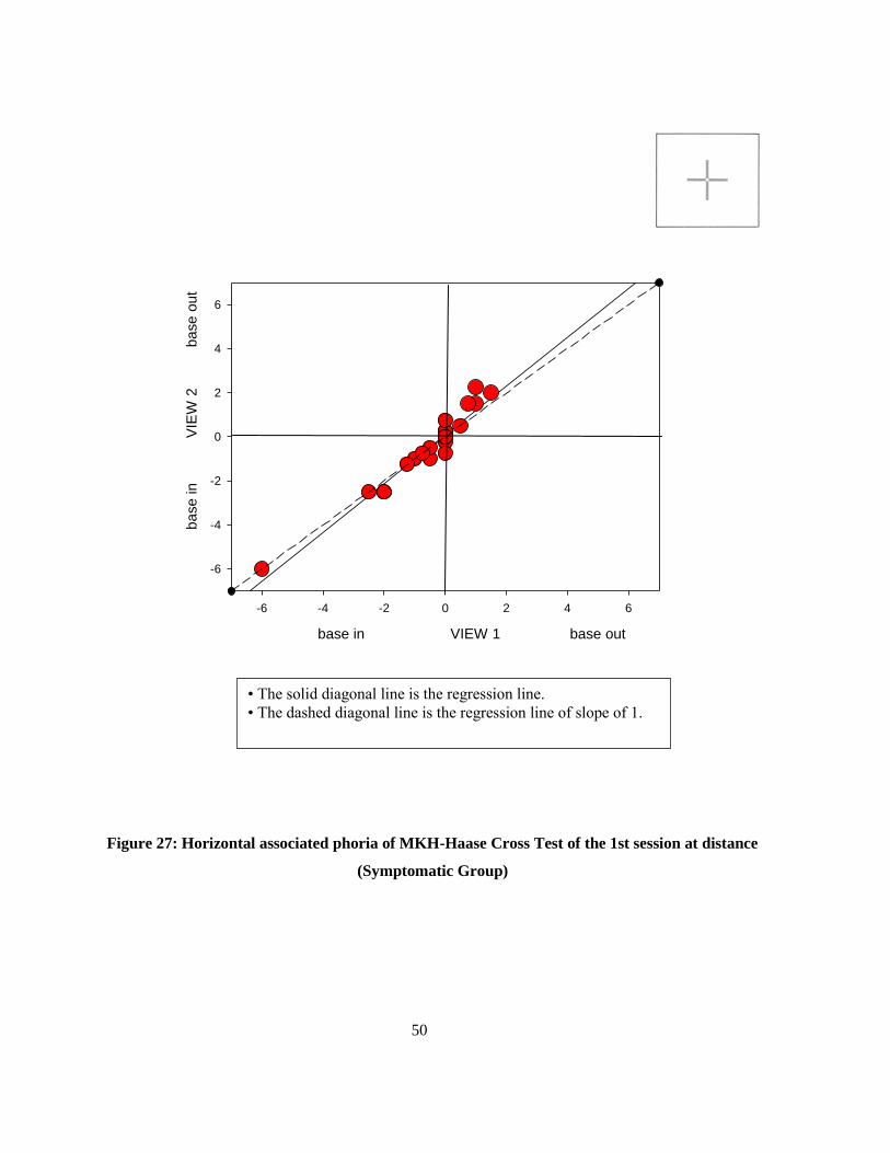
50
Figure 27: Horizontal associated phoria of MKH-Haase Cross Test of the 1st session at distance
(Symptomatic Group)
base in VIEW 1 base out
-6 -4 -2 0 2 4 6
base
in
V
IEW
2
ba
se
ou
t
-6
-4
-2
0
2
4
6
• The solid diagonal line is the regression line.
• The dashed diagonal line is the regression line of slope of 1.

51
Figure 28: Horizontal associated phoria of MKH-Haase Pointer Test of the 1st session at
distance
(Symptomatic Group)
base in VIEW 1 base out
-6 -4 -2 0 2 4 6
base in
V
IEW
2
b
ase o
ut
-6
-4
-2
0
2
4
6
• The solid diagonal line is the regression line.
• The dashed diagonal line is the regression line of slope of 1.

52
base down VIEW 1 base up
-1.0 -0.5 0.0 0.5 1.0
ba
se d
ow
n
V
IEW
2
b
ase u
p
-1.0
-0.5
0.0
0.5
1.0
Figure 29: Vertical associated phoria of MKH-Haase Rectangle Test of the 1st session at
distance
(Asymptomatic Group)
• The solid diagonal line is the regression line.
• The dashed diagonal line is the regression line of slope of 1.

53
6.1.1.2 Within the 1st session’s agreement of the MKH-Haase associated phoria charts at near:
Table 3 provides a summary of the results at near. With one exception, the agreement between
Views 1 and 2 was high based on the mean differences being statistically identical to zero and the
linear regression results that the slope and y-intercept were statistically identical to 1.0 and zero
respectively. The one exception was vertical associated phoria of Cross Test for the symptomatic
group. The reason that there was no correlation on this test was because nearly all of the symptomatic
groups’ subjects had a vertical associated phoria of zero for both Views 1 and 2 except for a few
subjects who an associated phoria between 0.25 and 0.50 Δ for one of the views (Figure 30).

54
Table 3: Mean difference, 95% CI, and linear regression of horizontal and vertical MKH-Haase
associated phoria charts at near (1st Session)
Subjects
Groups
Base
Direction Test Chart
Mean
Difference
(95 % CI)
Regression between View1 and View2
View 2 = b0 + (b1* View 1)
r
(p value)
Y-Intercept (b0)
(95 % CI)
Slope (b1)
(95% CI)
Sy
mp
tom
atic
Sub
ject
s
(N=
34
)
Ho
rizo
nta
l
Cross Test 0.029
(-0.04 to 0.01)
0.99
(p<0.001)
0.032
(-0.003 to 0.07)
1.03
(0.97 to 1.1)
Pointer Test -0.014
(-0.06 to 0.03)
0.99
(p<0.001)
-0.0159
(-0.023 to 0.012)
0.99
(0.92 to 1.2)
Double
Pointer Test
-0.007
(-0.05 to 0.03)
0.99
(p<0.001)
-0.0088
(-0.01 to 0.0042)
0.99
(0.93 to 1.01)
Ver
tica
l
Cross Test 0
(-0.03 to 0.03)
0.04
(p = 0.8) -- --
Double
Pointer Test 0 1 0 1
Rectangle
Test
-0.007
(-0.02 to 0.007)
0.97
(p<0.001)
-0.0075
(-0.0064 to 0.06)
0.97
(0.94 to 1.2)
Asy
mp
tom
atic
Sub
ject
s
(N=
40
)
Ho
rizo
nta
l
Cross Test 0 1 0 1
Pointer Test -0.0250
(-0.07 to 0.02)
0.97
(p<0.001)
-0.0367
(-0.054 to 0.032)
0.93
(0.83 to 1.04)
Double
Pointer Test
0.008
(-0.07 to 0.009)
0.91
(p<0.001)
-0.009
(-0.099 to 0.008)
0.99
(0.97 to 1.02)
Ver
tica
l
Cross Test 0
1 0 1
Double
Pointer Test 0 1 0 1
Rectangle
Test 0 1 0 1

55
Figure 30: Vertical associated phoria of MKH-Haase Cross Test of the 1st session at near
(Symptomatic Group)
base down (RE) VIEW 1 base up (RE)
-1.00 -0.75 -0.50 -0.25 0.00 0.25 0.50 0.75 1.00
base d
ow
n (
RE
)
VIE
W 2
base u
p (
RE
)
-1.00
-0.75
-0.50
-0.25
0.00
0.25
0.50
0.75
1.00
• The solid diagonal line is the regression line.
• The dashed diagonal line is the regression line of slope of 1.

56
6.1.1.3 Within the 2nd session agreement of the MKH-Haase associated phoria charts at
distance:
Table 4 is a summary for the View 1 and 2 comparisons for the second session at distance. There
are several trends to note. First, the linear regression results for the horizontal Pointer Test were
similar to the results in the first session. The associated phoria results for the symptomatic group were
more eso in View 2 for the lower exo and eso associated phorias measured in View 1. This result is
shown in Fig 31. Second, the trend for the lower exo and eso associated phoria to be more eso when
measured in View 2 were found in the Double Pointer Test results for both groups. The symptomatic
group results are shown in Fig 32 for illustration. Third, the result that the higher vertical associated
phorias measured using the Rectangle Test for the asymptomatic group decreased in magnitude when
the Polariods were switched to View 2 was repeated in the second session. Fourth, the correlation
between View 1 and 2 increased for the symptomatic group on the vertical Cross Test, but weaken on
the vertical Double Pointer and vertical Rectangle tests although all three tests had a slope for the
linear function that was statistically less than 1.0. This last result was due to the result that the
relatively larger vertical phorias measured in View 1 were reduced in View 2.
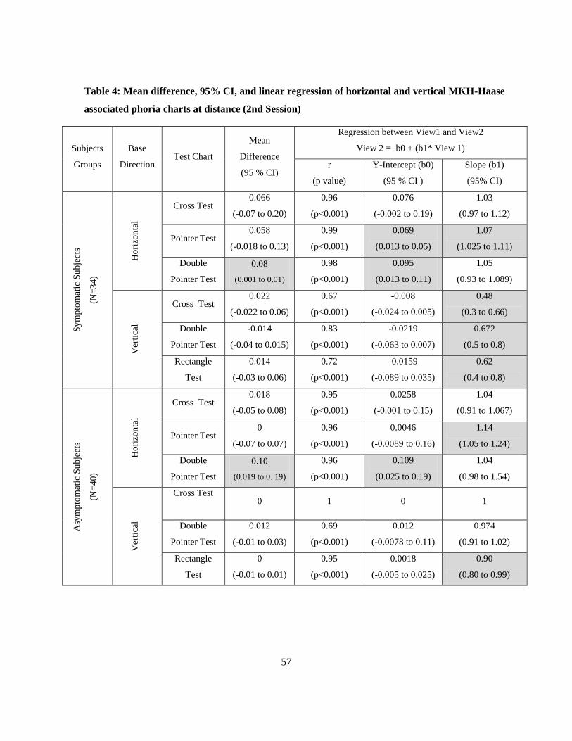
57
Table 4: Mean difference, 95% CI, and linear regression of horizontal and vertical MKH-Haase
associated phoria charts at distance (2nd Session)
Subjects
Groups
Base
Direction Test Chart
Mean
Difference
(95 % CI)
Regression between View1 and View2
View 2 = b0 + (b1* View 1)
r
(p value)
Y-Intercept (b0)
(95 % CI )
Slope (b1)
(95% CI)
Sy
mp
tom
atic
Su
bje
cts
(N=
34
)
Ho
rizo
nta
l
Cross Test 0.066
(-0.07 to 0.20)
0.96
(p<0.001)
0.076
(-0.002 to 0.19)
1.03
(0.97 to 1.12)
Pointer Test 0.058
(-0.018 to 0.13)
0.99
(p<0.001)
0.069
(0.013 to 0.05)
1.07
(1.025 to 1.11)
Double
Pointer Test
0.08
(0.001 to 0.01)
0.98
(p<0.001)
0.095
(0.013 to 0.11)
1.05
(0.93 to 1.089)
Ver
tica
l
Cross Test 0.022
(-0.022 to 0.06)
0.67
(p<0.001)
-0.008
(-0.024 to 0.005)
0.48
(0.3 to 0.66)
Double
Pointer Test
-0.014
(-0.04 to 0.015)
0.83
(p<0.001)
-0.0219
(-0.063 to 0.007)
0.672
(0.5 to 0.8)
Rectangle
Test
0.014
(-0.03 to 0.06)
0.72
(p<0.001)
-0.0159
(-0.089 to 0.035)
0.62
(0.4 to 0.8)
Asy
mp
tom
atic
Su
bje
cts
(N=
40
)
Ho
rizo
nta
l
Cross Test 0.018
(-0.05 to 0.08)
0.95
(p<0.001)
0.0258
(-0.001 to 0.15)
1.04
(0.91 to 1.067)
Pointer Test 0
(-0.07 to 0.07)
0.96
(p<0.001)
0.0046
(-0.0089 to 0.16)
1.14
(1.05 to 1.24)
Double
Pointer Test
0.10
(0.019 to 0. 19)
0.96
(p<0.001)
0.109
(0.025 to 0.19)
1.04
(0.98 to 1.54)
Ver
tica
l
Cross Test
0 1 0 1
Double
Pointer Test
0.012
(-0.01 to 0.03)
0.69
(p<0.001)
0.012
(-0.0078 to 0.11)
0.974
(0.91 to 1.02)
Rectangle
Test
0
(-0.01 to 0.01)
0.95
(p<0.001)
0.0018
(-0.005 to 0.025)
0.90
(0.80 to 0.99)

58
Figure 31: Horizontal associated phoria of MKH-Haase Pointer Test of the 2nd session at
distance
(Symptomatic Group)
base in VIEW 1 base out
-8 -6 -4 -2 0 2 4 6 8
base in
V
IEW
2
b
ase o
ut
-8
-6
-4
-2
0
2
4
6
8
• The solid diagonal line is the regression line.
• The dashed diagonal line is the regression line of slope of 1.
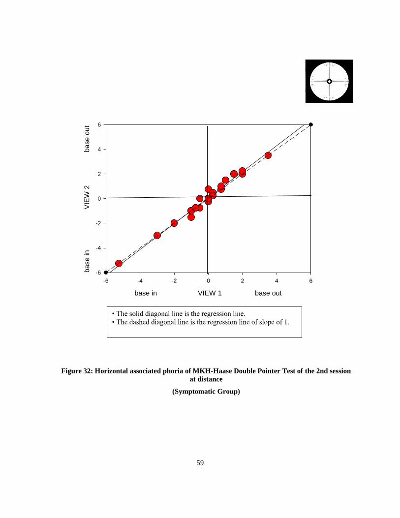
59
Figure 32: Horizontal associated phoria of MKH-Haase Double Pointer Test of the 2nd session
at distance
(Symptomatic Group)
base in VIEW 1 base out
-6 -4 -2 0 2 4 6
base in
V
IEW
2
b
ase o
ut
-6
-4
-2
0
2
4
6
• The solid diagonal line is the regression line.
• The dashed diagonal line is the regression line of slope of 1.

60
6.1.1.4 Within the 2nd session agreement of the MKH-Haase associated phoria charts at near:
Table 5 shows the comparisons of View 1 and 2 for near at the second session. Similar to the first
session at near, the horizontal phorias showed excellent agreement with the mean differences being
statistically identical to zero and the linear regression results that the slope and y-intercept were
statistically identical to 1.0 and zero respectively. Unlike the first session, all three vertical associated
phoria tests for the symptomatic group had excellent correlations. Both the Cross Test and Rectangle
Test also had a slope of 1.0 and a y-intercept of zero. The slope of the regression for the Double
Pointer Test, however, was significantly less than 1.0. This last result was due to the result that the
relatively larger vertical phorias measured in View 1 were reduced in View 2.

61
Table 5: Mean difference, 95% CI, and linear regression of horizontal and vertical MKH-Haase
associated phoria charts at near (2nd Session)
Subjects
Groups
Base
Direction Test Chart
Mean
Difference
(95 % CI)
Regression between View1 and View2
View 2 = b0 + (b1* View 1)
r
(p value)
Y-Intercept (b0)
(95 % CI)
Slope (b1)
(95% CI)
Sym
pto
mat
ic S
ubje
cts
(N=
34)
Ho
rizo
nta
l
Cross Test -0.014
(-0.06 to 0.03)
0.95
(p<0.001)
-0.0149
(-0.0025 to 0.05)
0.99
(0.96 to 1.3)
Pointer Test 0.051
(-0.008 to 0.1)
0.99
(p<0.001)
0.054
(-0.099 to 0.085)
1.003
(0.97 to 1.1)
Double
Pointer Test
0
(-0.04 to 0.04)
0.99
(p<0.001)
0.001
(-0.087 to 0.099)
1.002
(0.94 to 1.09)
Ver
tica
l
Cross Test -0.02
(-0.06 to 0.02)
0.99
(p<0.001)
-0.0239
(-0.003 to 0.006)
0.93
(0.89 to 1.1)
Double
Pointer Test -0.0073
(-0.02 to 0.007) 0.92
(p<0.001)
-0.0109
(-0.01 to 0.0056)
0.83
(0.72 to 0.94)
Rectangle
Test 0.007
(-0.007 to 0.02) 0.96
(p<0.001)
0.0047
(-0.0085 to 0.0065)
0.94
(0.90 to 1.2)
Asy
mpto
mat
ic S
ubje
cts
(N=
40)
Hori
zonta
l
Cross Test -0.04
(-0.1 to 0.03)
0.94
(p<0.001)
-0.0573
(-0.025 to 0.0075)
0.90
(0.86 to 1.089)
Pointer Test 0
1 0 1
Double
Pointer Test
0.012
(-0.01 to 0.03)
0.99
(p<0.001)
0.011
(-0.055 to 0.045)
0.99
(0.92 to 1.3)
Ver
tica
l
Cross Test 0
1 0 0
Double
Pointer Test 0 1 0 0
Rectangle
Test 0 1 0 1

62
6.1.2 Discussion:
MKH-Haase method protocol requires the associated phoria to be measured twice within a
session; once with the Polariods oriented with their axes at 45o and 135
o (View 1) and again with the
axes switched (View 2). The purpose of this study was to look at the correlation between the two
measurements within the first and the second sessions at both distance and near for each test chart.
First, in most of cases, the mean differences between View 1 and View 2 of horizontal associated
phoria were less than a 0.25 Δ. The mean differences of vertical associated phorias were also small
and less than 0.25 Δ. These small differences are not considered clinically significant.
In addition to the mean difference comparisons, the linear regressions between View 1 and View 2
were calculated as well in order to determine whether there is a bias for one view presentation over
the other. We wanted to know if the slope and y-intercept of the regressions were statistically
significantly different from zero. For the majority of tests at distance, there was a strong linear
correlation with slopes statistically identical to 1.0 and the y-intercept statistically identical to zero.
Nevertheless, there were some exceptions. The exceptions for the horizontal associated phoria
followed two general patterns. One was that larger associated values measured in View 1 tended to
increase in View 2 especially for the eso values, and the other pattern was that the low exo and eso
associated phorias became slightly more eso when the axis was switched. Again, the differences were
less than 0.25 or 0.50 and are not considered to be clinically important.
The correlation between View 1 and 2 were more varied across tests and sessions for the vertical
associated phorias. Although there was no systematic difference between the means of View 1 and 2,
the regressions (if significant) showed that the larger associated phorias measured in View 1
decreased when the images to each eye were switched. Again, these amounts were small and the
change was often no greater than 0.25 Δ. In addition, the magnitude of the vertical associated phoria

63
was rarely greater than 0.25 Δ suggesting the varied results found for the vertical associated phorias
regressions were an artifact due to a small range of values.
From one perspective, these differences between View 1 and 2 are small and could be clinically
unimportant. It is also possible that the statistically significant differences between the two views
could be a spurious finding given the number of comparisons performed. Nevertheless, the
repeatability of the horizontal differences between View 1 and 2 found for the Pointer Test and the
vertical differences found for the Rectangle Test suggest that there may be subtle differences between
the two types of presentation at least at distance. The clinical importance of these findings is
uncertain.
One possible explanation is the design of the tests. The Cross Test does not have a central fusion
lock but the Pointer and Double Pointer Tests do have central fusion locks. In addition, the angular
size of the Cross Test lines is smaller than Pointer and Double Pointer Tests. Moreover, there are
more central and peripheral details with the Double Pointer Test than the Pointer Test, which may
contribute to the variability results between those tests. Previous studies showed that fixation
disparity is significantly affected when measured with or without a target with a central fusion lock.
The angular size of the fusion lock was considered an important factor for people who have visual
symptoms (Carter, 1964a; Saladin & Carr, 1983; Wildsoet & Cameron, 1985).
Results showed that subjects with high associated phoria in View 1 chart became higher when the
polarized axes were switched to View 2. This was more likely to occur with the symptomatic group
and at the second session. This difference between the associated phorias was not present at near for
either group. It is possible that the results were due to prism adaptation. The correcting prisms were
removed before the axes were switched and then associated phoria was re-measured starting with zero
prisms. The time required to re-measure the associated phorias in View 2 may not have been
sufficient to allow for any decay of any prism adaptation that occurred with View 1; however,

64
assuming that the time course for prism adaptation was the same at distance and near, one would have
also expected this to occur at near, which it did not. The other finding that suggests that this
difference between View 1 and View 2 was probably due to prism adaptation was the associated
vertical phorias. If there was a systematic difference between View 1 and View 2, the effect was that
the vertical associated phoria was less for the second presentation, which is inconsistent with prism
adaptation.
The finding that the differences between presentations were more likely to occur at distance raises
the issue as to whether there is something different about the distance test screen. The distance screen
sat on a small table and the angle of the screen was adjusted to be perpendicular to the subject’s line
of sight using the self-contained level. The near unit, however, was often hand held and the angle
between display and line of sight was not always constant. As will be described later, the tilt of either
display, but particularly the distance chart, does affect the relative position of the dichoptic targets.
Subtle changes in the subject’s line of sight with the distance chart could be responsible for the small
differences found in this study.

65
6.2 Between-session repeatability of the MKH-Haase associated phoria charts:
Although there were some differences between View 1 and View 2 presentations within a
session, I will average these within session results for determining the repeatability between sessions.
The primary reason for averaging was that the differences between View 1 and View 2 within a
session were generally small. The between-session repeatability was conducted by the same statistical
methods of the within session agreement.
6.2.1 Results:
6.2.1.1 Between-Session Repeatability of MKH-Haase associated phoria charts at distance
(Session1 vs. Session2):
Table 6 summarizes the results. None of the mean differences between the two sessions (Session 2
– Session 1) were statistically significant from zero. The linear regression between the horizontal
values was strong, whereas the vertical associated phoria linear regressions between the two sessions
were generally not significant. This last result was because nearly everyone had a vertical associated
phoria within +0.125 Δ of zero for both sessions.
For the majority of the horizontal associated phoria, the slopes were statistically identical to 1.0
and the y-intercepts were statistically identical to zero. The exceptions are the shaded cells. Figure 33
shows the scatter plot of the symptomatic group’s results for the Pointer Test. The slope was slightly
less than 1.0 because the larger associated phorias decreased slightly at the second session. The
results of Pointer and Double Pointer Tests showed that for most of subjects who had high exo
associated phoria values of Session 2 they were more exo with Session 1 presentation. However, most
of subjects who had moderate exo associated phoria values of Session 2 they were less exo with
Session 1 presentation.
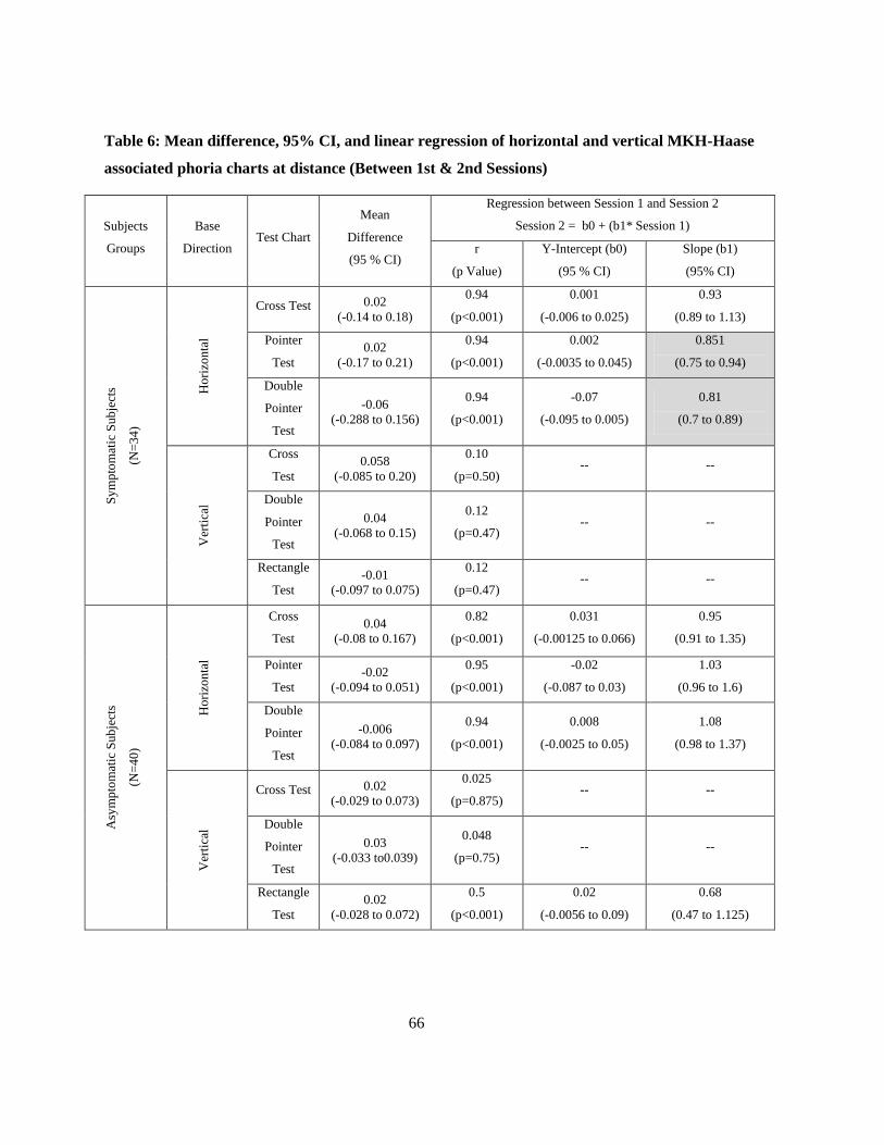
66
Table 6: Mean difference, 95% CI, and linear regression of horizontal and vertical MKH-Haase
associated phoria charts at distance (Between 1st & 2nd Sessions)
Subjects
Groups
Base
Direction Test Chart
Mean
Difference
(95 % CI)
Regression between Session 1 and Session 2
Session 2 = b0 + (b1* Session 1)
r
(p Value)
Y-Intercept (b0)
(95 % CI)
Slope (b1)
(95% CI)
Sy
mp
tom
atic
Sub
ject
s
(N=
34
)
Ho
rizo
nta
l
Cross Test 0.02
(-0.14 to 0.18)
0.94
(p<0.001)
0.001
(-0.006 to 0.025)
0.93
(0.89 to 1.13)
Pointer
Test
0.02
(-0.17 to 0.21)
0.94
(p<0.001)
0.002
(-0.0035 to 0.045)
0.851
(0.75 to 0.94)
Double
Pointer
Test
-0.06
(-0.288 to 0.156)
0.94
(p<0.001)
-0.07
(-0.095 to 0.005)
0.81
(0.7 to 0.89)
Ver
tica
l
Cross
Test
0.058
(-0.085 to 0.20)
0.10
(p=0.50) -- --
Double
Pointer
Test
0.04
(-0.068 to 0.15)
0.12
(p=0.47) -- --
Rectangle
Test
-0.01
(-0.097 to 0.075)
0.12
(p=0.47) -- --
Asy
mp
tom
atic
Sub
ject
s
(N=
40
)
Ho
rizo
nta
l
Cross
Test
0.04
(-0.08 to 0.167)
0.82
(p<0.001)
0.031
(-0.00125 to 0.066)
0.95
(0.91 to 1.35)
Pointer
Test
-0.02
(-0.094 to 0.051)
0.95
(p<0.001)
-0.02
(-0.087 to 0.03)
1.03
(0.96 to 1.6)
Double
Pointer
Test
-0.006
(-0.084 to 0.097)
0.94
(p<0.001)
0.008
(-0.0025 to 0.05)
1.08
(0.98 to 1.37)
Ver
tica
l
Cross Test 0.02
(-0.029 to 0.073)
0.025
(p=0.875) -- --
Double
Pointer
Test
0.03
(-0.033 to0.039)
0.048
(p=0.75) -- --
Rectangle
Test
0.02
(-0.028 to 0.072)
0.5
(p<0.001)
0.02
(-0.0056 to 0.09)
0.68
(0.47 to 1.125)

67
Figure 33: Between-session repeatability of horizontal associated phoria of MKH-Haase Pointer
Test at distance
(Symptomatic Group)
base in SESSION 1 base out
-6 -4 -2 0 2 4 6
ba
se
in
S
ES
SIO
N 2
ba
se
ou
t
-6
-4
-2
0
2
4
6
• The solid diagonal line is the regression line.
• The dashed diagonal line is the regression line of slope of 1.

68
6.2.1.2 Between-Session Repeatability of MKH-Haase associated phoria charts at near
(Session1 vs. Session2):
Table 7 summarizes the results. None of the mean differences between the two sessions (Session 2
– Session 1) were statistically significant from zero. The linear regression between the horizontal
values was strong for the symptomatic group and low to moderate for the asymptomatic group. Most
of the vertical tests did not have a significant correlation between the two sessions. The exception
was the Rectangle Test of the asymptomatic group. The correlation was moderate and significant.
This last result was because nearly everyone had a vertical associated phoria within +0.125 Δ of zero
for both sessions.
Figure 34 show the scatter plot of the symptomatic group’s results for the Cross Test. The slopes
of the regression were slightly less than 1.0. The lower value for the slope was a result of the subjects
who had high exo associated phoria values in Session 1 and a lower exo (more eso) value in Session
2. The Cross Test for the asymptomatic group showed low correlation between the two sessions. This
was due to the relatively large differences between the two sessions for a few subjects (e.g., Session 1
was -1.00 , and Session 2 was 0.50 Δ). Otherwise, most of subjects had either identical or small
differences between the two sessions.
The vertical linear regressions between sessions were generally not significant, except for the
Rectangle Test of the asymptomatic group. The main reason for the lack of significant regressions for
the vertical tests was that most of the subjects had no associated vertical phoria at both sessions or the
between-session difference was small. Although the correlation was not strong, for the asymptomatic
group the larger vertical associated phoria at the first session decreased in magnitude at the second
session (Figure 35).

69
Table 7: Mean difference, 95% CI, and linear regression of horizontal and vertical MKH-Haase
associated phoria charts at near (Between 1st & 2nd Sessions)
Subjects
Groups
Base
Direction Test Chart
Mean
Difference
(95 % CI)
Regression between Session 1 and Session 2
Session 2 = b0 + (b1* Session 1)
r
(p Value)
Y-Intercept (b0)
(95 % CI)
Slope (b1)
(95% CI)
Sy
mp
tom
atic
Su
bje
cts
(N=
34
)
Ho
rizo
nta
l
Cross Test -0.029
(-0.27 to 0.32)
0.85
(p<0.001)
-0.047
(-0.1 to 0.065)
0.75
(0.6 to 0.9)
Pointer Test -0.091
(-0.43 to 0.24)
0.83
(p<0.001)
-0.27
(-0.47 to 0.0098)
0.7
(0.55 to 0.85)
Double
Pointer Test
-0.091
(-0.43 to 0.24)
0.84
(p<0.001)
-0.27
(-0.51 to 0.0098)
0.74
(0.57 to 0.89)
Ver
tica
l
Cross Test -0.025
(-0.072 to 0.020)
0.1
(p=0.5) -- --
Double
Pointer Test
-0.003
(-0.054 to 0.047)
0.05
(p=0.7) -- --
Rectangle
Test
-0.036
(-0.12 to 0.054)
0.33
(p=0.056) -- --
Asy
mp
tom
atic
Su
bje
cts
(N=
40
)
Ho
rizo
nta
l
Cross Test -0.09
(-0.349 to 0.168)
0.320
(p<0.004)
-0.136
(-0.45 to 0.025)
0.39
(0.04 to 0.47)
Pointer Test -0.106
(-0.30 to 0.094)
0.62
(p<0.001)
-0.15
(-0.67 to 0.074)
0.73
(0.4 to 1.04)
Double
Pointer Test
-0.073
(-0.26 to 0.12)
0.64
(p<0.001)
-0.10
(-0.34 to 0.045)
0.82
(0.72 to 1.08)
Ver
tica
l
Cross Test 0
NA NA NA
Double
Pointer Test
-0.012
(-0.03 to 0.005)
0.025
(p=0.87) -- --
Rectangle
Test
-0.025
(-0.072 to 0.022)
0.43
(p=0.005)
-0.009
(-0.063 to 0.035)
0.183
(0.006 to 0.3)
NA: Session 1 and Session 2 results equal to zero for each subject.

70
Figure 34: : Between-session repeatability of horizontal associated phoria of MKH-Haase Cross
Test at near
(Symptomatic Group)
base in SESSION 1 base out
-8 -6 -4 -2 0 2 4 6 8
ba
se
in
SE
SS
ION
2
b
ase
ou
t
-8
-6
-4
-2
0
2
4
6
8
• The solid diagonal line is the regression line.
• The dashed diagonal line is the regression line of slope of 1.

71
Figure 35: Between-session repeatability of vertical associated phoria of MKH-Haase Rectangle
Test at near
(Asymptomatic Group)
base down SESSION 1 base up
-1.0 -0.5 0.0 0.5 1.0ba
se
do
wn
SE
SS
ION
2
b
ase
up
-1.0
-0.5
0.0
0.5
1.0
• The solid diagonal line is the regression line.
• The dashed diagonal line is the regression line of slope of 1.

72
6.2.2 Discussion:
The mean differences between Session 1 and Session 2 were not significantly different from zero
for all associated phoria tests at both distance and near. However, regression results showed some
significant trends in the horizontal associated phoria results for the symptomatic group on the Pointer
and Double Pointer tests. For the larger associated phorias, the magnitude at the second session
tended to be less than the first session value. However, most of differences between the two sessions
were less than 0.25 Δ.
At near, most of the horizontal associated phoria tests showed a high correlation between the two
sessions. The Pointer and Double Pointer tests also showed the reduction in magnitude of the higher
horizontal associated phoria values at the second session. The one exception to the strong correlation
was the asymptomatic group's Cross Test results.
The correlations between the two sessions for the majority of vertical associated phorias tests were
low and non-significant. This occurred because the values for the both sessions were zero for nearly
everyone. The one exception was the Rectangle Test for asymptomatic group at both distance and
near. The correlation between the two sessions for that test was moderate.
Between-session repeatability of MKH-Haase associated phoria tests were conducted by
computing the 95% limits of agreement according to Bland & Altman method of repeatability (Bland
& Altman, 1986; Bland & Altman, 1995). Tables 8 and 9 show the 95% limits of agreement between
different horizontal and vertical MKH-Haase associated phoria tests at both distance and near
respectively. Associated phoria values were rounded to the closest 0.25 step for horizontal tests,
and to the closest 1/8 step for vertical tests.

73
Table 8: Between-session repeatability of MKH-Haase associated phoria tests at distance:
(Session1 vs. Session2)
Subjects
Groups
Base
Direction
Test
Chart
Coefficient of
Repeatability
(1.96SD)
95% Limits of Agreement
Sym
pto
mat
ic S
ubje
cts
(N=
34)
Ho
rizo
nta
l
Cross
Test 0.92 -1.00 to 1.00
Pointer
Test 1.08 -1.00 to 1.18
Double Pointer
Test 1.25 -1.25 to 1. 25
Ver
tica
l
Cross
Test 0.78 -0.75 to 0.86
Double Pointer
Test 0.63 -0.68 to 0.50
Rectangle
Test 0.50 -0.50 to 0.50
Asy
mpto
mat
ic S
ubje
cts
(N=
40)
Hori
zonta
l
Cross
Test 0.80 -0.75 to 0.75
Pointer
Test 0.45 -0.50 to 0.50
Double Pointer
Test 1.70 -1.75 to 1.75
Ver
tica
l
Cross
Test 0.30
-0.25 to 0.25
Double Pointer
Test 0.20 -0.25 to 0.25
Rectangle
Test 0.30 -0.25 to 0.25

74
Table 9: Betweensession repeatability of MKH-Haase associated phoria tests at near: (Session1
vs. Session2)
Subjects
Groups
Base
Direction
Test
Chart
Coefficient of
Repeatability
(1.96SD)
95% Limits of Agreement
Sym
pto
mat
ic S
ubje
cts
(N=
34)
Ho
rizo
nta
l
Cross
Test 1.68 -1.75 to 1.75
Pointer
Test 1.90 -1.75 to 2.00
Double Pointer
Test 1.90 -1.75 to 2.00
Ver
tica
l
Cross
Test 0.25 -0.25 to 0.25
Double Pointer
Test 0.30 -0.25 to 0.25
Rectangle
Test 0.33 -0.25 to 0.37
Asy
mpto
mat
ic S
ubje
cts
(N=
40)
Hori
zonta
l
Cross
Test 1.56 -1.50 to 1.75
Pointer
Test 1.24 -1.25 to 1.25
Double Pointer
Test 1.20 -1.25 to 1.25
Ver
tica
l
Cross
Test 0.22 -0.25 to 0.25
Double Pointer
Test 0.09 -0.12 to 0.12
Rectangle
Test 0.30 -0.25 to 0.25

75
6.3 Within session agreement of the MKH-Haase stereoacuity tests:
The objectives of this study were to determine the correlation between crossed and uncrossed
disparities of the MKH-Haase stereoacuity tests. The MKH-Haase test protocol requires the
stereoacuity to be measured twice within a session; once with the Polariods oriented with their axes at
45o and 135
o and again with the axes switched. This switch provides the capability of measuring
crossed and uncrossed disparity stereothreshold. Before comparing the results between tests and
sessions, I will first exam the agreement between MKH-Haase stereoacuity measurements for the two
disparities of presentations within each of the first and second sessions.
The data were examined by using linear regression between log values of the crossed and
uncrossed stereothresholds for each test. Means differences between the log values of uncrossed and
crossed disparities (uncrossed – crossed values) along with the 95 % confidence interval for each test
were also calculated to determine whether there was a bias for one of the disparities. Statistical
decisions were based on the 95% confidence intervals unless stated otherwise.
6.3.1 Results:
6.3.1.1 Within the 1st session agreement of the MKH-Haase stereoacuity charts at distance:
Table 10 summarizes the results for the Line and Step Tests at distance. Six symptomatic subjects
and 9 asymptomatic subjects could not identify the maximum disparity of the Step Test and were
excluded from this analysis. A positive mean difference indicates that the threshold for crossed
disparities was lower than uncrossed disparities. The shaded cells in Table 8 highlight the tests where
the mean difference was significantly different from zero. This was the Line Test for the symptomatic
group and the Step Test of the asymptomatic group.
The correlation between the two types of disparities was reasonable. Based on the slope and y-
intercept values for the symptomatic subjects the Line and the Step tests did not vary as a function of
the disparity magnitude. The asymptomatic subjects’ results for the Line Test did have some

76
differences between the crossed and uncrossed disparities. Figure 36 is the scatter plot of these
results. For this test, subjects with the larger crossed disparity thresholds tended to have relatively
lower uncrossed thresholds, whereas the subjects with the lower crossed disparities tended to have
relatively higher uncrossed thresholds.
Table 10: Mean difference, 95% CI, and linear regression values of the 1st session of MKH-
Haase stereothreshold values at distance (crossed vs. uncrossed disparities)
Subjects
Groups
Test
Chart
Log Mean
Difference
(95 % CI)
Regression between Crossed and Uncrossed Disparity
Log Uncrossed Disparity = b0 + (b1* Log Crossed Disparity)
r
(p value)
Y-Intercept
(b0)
(95 % CI)
Slope (b1)
(95% CI)
Symptomatic
Subjects
Line
Test
(N=34)
0.112
(0.003 to 0.22)
0.743
(p< 0.001)
0.241
(-0.7 to 0.5)
0.90
(0.63 to 1.17)
Step
Test
(N=28)
0.055
(-0.038 to 0.15)
0.52
(p=0.005) )
0.561
(-0.2 to 0.6)
0.68
(0.28 to 1.11)
Asymptomatic
Subjects
Line
Test
(N=40)
0.022
(-0.04 to 0.09)
0.78
(p< 0.001)
0.37
( 0.1 to 0.64)
0.75
(0.56 to 0.94)
Step
Test
(N=31)
0.126
(0.04 to 0.21)
0.6
(p< 0.001)
0.49
(-0.35 to 0.59)
0.77
(0.42 to 1.12)

77
Figure 36: Within the 1st session agreement of MKH-Haase Line Stereotest at distance
(Asymptomatic Group)
(Crossed Disparity vs. Uncrossed Disparity)
CROSSED DISPARITY (Log Second of Arc)
0.0 0.5 1.0 1.5 2.0 2.5
UN
CR
OS
SE
D D
ISP
AR
ITY
(Log S
econd o
f A
rc)
0.0
0.5
1.0
1.5
2.0
2.5
• The solid diagonal line is the regression line.
• The dashed diagonal line is the regression line of slope of 1.

78
Table 11 lists the number of subjects who correctly identified “the Hand” in the Hand Random
dot Stereotest. This test only measures the presence or absence of global stereopsis. This test is
relatively challenging in that less than 45% of the subjects were able to perceive the hand form for
both directions. The majority were either unable to perceive the form at all or could only perceive
form in one direction (the number of subjects who saw only crossed disparity and uncrossed disparity
were pooled together). The distribution of the frequencies between the two subject groups was not
statistically significant (X2=0.5, DF =2, and p=0.77).
Table 11: Within the 1st session repeatability of MKH-Haase Hand Test at distance (crossed vs.
uncrossed)
Groups
Number of
subjects who saw
both disparities
Number of
subjects who
were unable to
detect either
Disparity
Number of
subjects who
saw only the
crossed disparity
Number of
subjects who saw
only the
uncrossed
disparity
Symptomatic
Group
(N=34)
11
(33 %)
15
(44%)
6
(17%)
2
(5.8%)
Asymptomatic
Group
(N=40)
17
(42.5%)
16
(40%)
7
(17.5%) 0
6.3.1.2 Within the 1st session agreement of the MKH-Haase stereoacuity charts at near:
Table 12 summarizes the crossed and uncrossed disparity results. Three subjects from the
symptomatic group failed to distinguish the maximum disparity of Step Test and were excluded from
the analysis. None of the mean differences were significantly different from zero.
The results showed high and significant correlation between crossed and uncrossed disparities for
both tests. Similar to the distance findings, correlations between crossed and uncrossed disparities
were higher with the Line Test than the Step Test. For all of the tests, the slopes were statistically
identical to 1.0 and the y-intercepts were statistically identical to zero.

79
Table 12: Mean difference, 95% CI, and linear regression values of the 1st session of MKH-
Haase stereothreshold values at near (crossed vs. uncrossed disparities)
Subjects
Groups
Test
Chart
Log Mean
Difference
(95 % CI)
Regression between Crossed and Uncrossed Disparity
Log Uncrossed Disparity = b0 + (b1* Log Crossed Disparity)
r
(p Value)
Y-Intercept (b0)
(95 % CI)
Slope (b1)
(95% CI)
Symptomatic
Subjects
Line
Test
(N=34)
0.014 (-0.006 to 0.03)
0.88
(p<0.001)
-0.103
(-1.23 to 0.2)
1.11
(0.87 to 1.57)
Step
Test
(N=31)
0.02 (-0.003 to 0.06)
0.71
(p<0.001)
0.13
(-0.85 to 1.1)
0.92
(0.73 to 1.25)
Asymptomatic
Subjects
Line
Test
(N=40)
-0.0075 (-0.02 to 0.007)
1
0.387
(-0.79 to 0.98)
0.613
(0.25 to 1.1)
Step
Test
(N=40)
0.0075 (-0.019 to0.034)
0.90
(p<0.001)
0.12
(-0.4 to 0.87)
0.92
(0.79 to 1.06)
6.3.1.3 Within the 2nd session agreement of the MKH-Haase stereoacuity charts at distance:
Table 13 summarizes the results for the Step and Line tests at distance. Seven symptomatic
subjects and six asymptomatic subjects failed to distinguish the maximum disparity of Step Test at
distance and were excluded from this analysis. A positive mean difference indicates that the threshold
for crossed disparities was lower than uncrossed disparities. The shaded cells in table 11 highlight the
tests were the mean difference was significantly different from zero. This was for the Step Test for
both groups. For the majority of the tests, the slopes were statistically identical to 1.0 and the y-
intercepts were statistically identical to zero. The exception is the Line Test of the asymptomatic
group (the shaded cell in table 8). The result was similar to the first session results. Figure 37 is the

80
scatter plot of these results. The slope’s data set was slightly less than 1.0 and y-intercept was higher
than zero. For this test, subjects with the larger crossed disparity thresholds tended to have relatively
lower uncrossed thresholds, whereas the subjects with the lower crossed disparities tended to have
relatively higher uncrossed thresholds.
Table 13: Mean difference, 95% CI, and linear regression values of the 2nd session of MKH-
Haase stereothreshold values at distance (crossed vs. uncrossed disparities)
Subjects
Groups
Test
Chart
Log Mean
Difference
(95 % CI)
Regression between Crossed and Uncrossed Disparity
Log Uncrossed Disparity = b0 + (b1* Log Crossed Disparity)
r
(p value)
Y-Intercept (b0)
(95 % CI)
Slope (b1)
(95% CI)
Symptomatic
Subjects
Line
Test
(N=34)
0.106
(-0.0009 to 0.2)
0. 76
(p<0.001)
0.186
(-0.23 to 0.28)
0.94
(0.64 to 1.2)
Step
Test
(N=27)
-0.064
(-0.001 to -0.12)
0.64
(p<0.001)
0.29
(-0.56 to 0.85)
0.85
(0.35 to 1.1)
Asymptomatic
Subjects
Line
Test
(N=40)
0.037
(-0.065 to 0.14)
0.63
(p<0.001)
0.5
(0.11 to 0.89)
0.67
(0.42 to 0.93)
Step
Test
(N=34)
0.045 (0.0001 to 0.09)
0.84
(p<0.001)
0.15
(-0.35 to 0.45)
0.93
(0.78 to 1.16)
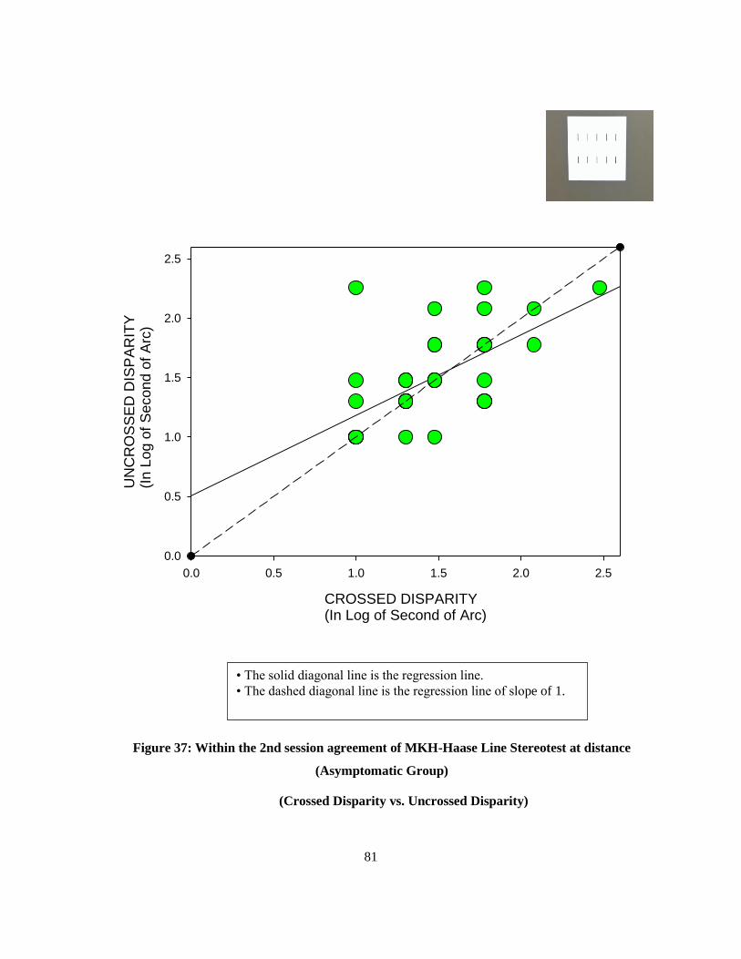
81
Figure 37: Within the 2nd session agreement of MKH-Haase Line Stereotest at distance
(Asymptomatic Group)
(Crossed Disparity vs. Uncrossed Disparity)
CROSSED DISPARITY(In Log of Second of Arc)
0.0 0.5 1.0 1.5 2.0 2.5
UN
CR
OS
SE
D D
ISP
AR
ITY
(In L
og o
f S
econd o
f A
rc)
0.0
0.5
1.0
1.5
2.0
2.5
• The solid diagonal line is the regression line.
• The dashed diagonal line is the regression line of slope of 1.

82
Table 14 provides information about the number of subjects who correctly identified “the hand”
with Hand Random dot Stereotest. Approximately 50% from both groups of the subjects were able to
perceive form for both directions. The other half of subjects were either unable to perceive the form at
all or could only perceive form for one direction (the number of subjects who saw only crossed
disparity and uncrossed disparity were pooled together). The distribution of the frequencies between
the two subject groups was not statistically significant (X2=0.74, DF =2, and p=0.68).
Table 14: Within the 2nd Session repeatability of MKH-Haase Hand test at distance (crossed vs.
uncrossed)
Groups
Number of
subjects who
saw both
disparities
Number of
subjects who
were unable to
detect either
disparity
Number of
subjects who
saw only the
crossed disparity
Number of
subjects who saw
only the
uncrossed
disparity
Symptomatic
Group
(N=34)
18
(52.9 %)
15
(44%)
1
(2.9%) 0
Asymptomatic
Group
(N=40)
20
(50%)
17
(42.5%)
2
(5%)
1
(2.5%)
6.3.1.4 Within the 2nd session agreement of the MKH-Haase stereoacuity charts at near:
Table 15 summarizes the crossed and uncrossed disparity results. Two subjects from the
symptomatic group failed to perceive the maximum stereothreshold of the Step Test and they have
been excluded from the analysis. None of the mean differences were significantly different from zero.
The results showed high and significant correlation between crossed and uncrossed disparities for
both tests. Regression of the Step Test of the asymptomatic group was not as high as other tests. For
the asymptomatic group, the slopes were statistically identical to 1.0 and the y-intercepts were
statistically identical to zero for both tests. The slope was less than 1.0 and y-intercept was higher
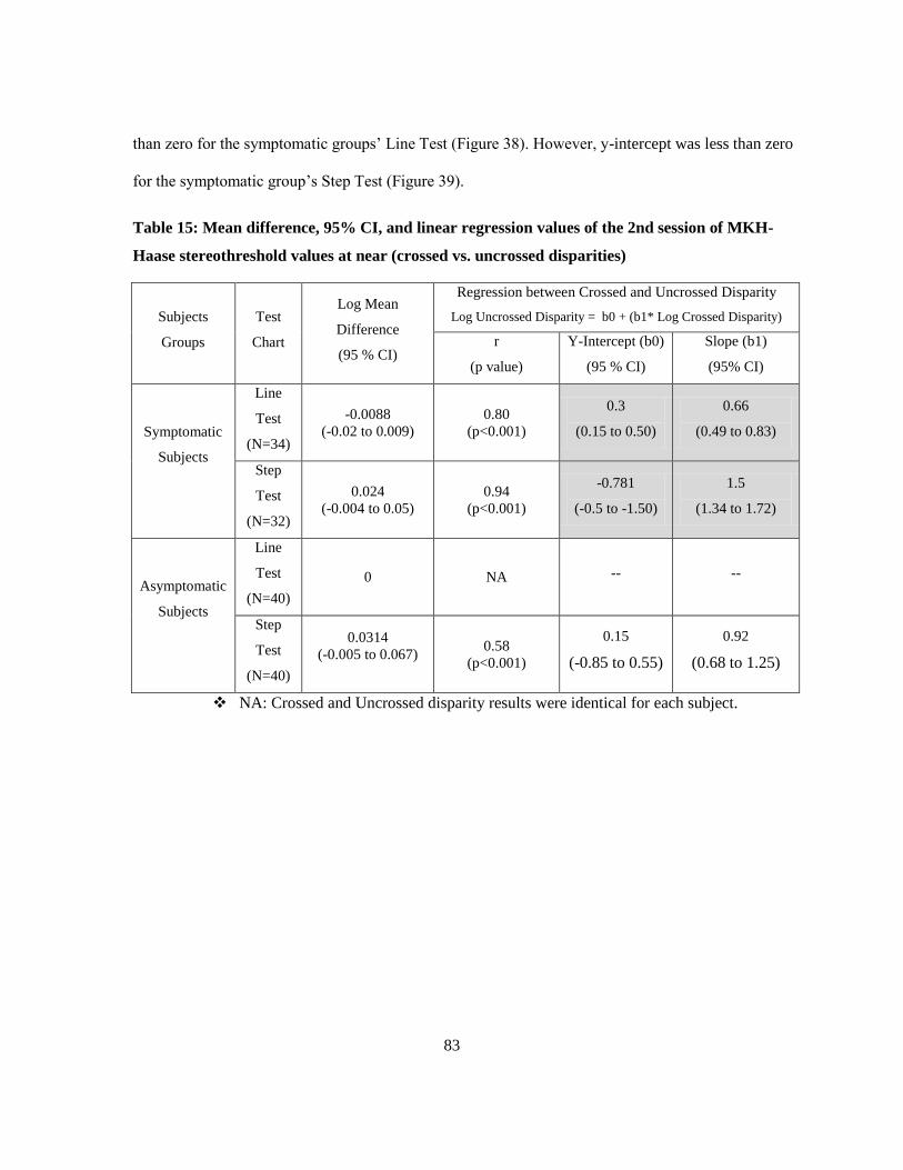
83
than zero for the symptomatic groups’ Line Test (Figure 38). However, y-intercept was less than zero
for the symptomatic group’s Step Test (Figure 39).
Table 15: Mean difference, 95% CI, and linear regression values of the 2nd session of MKH-
Haase stereothreshold values at near (crossed vs. uncrossed disparities)
Subjects
Groups
Test
Chart
Log Mean
Difference
(95 % CI)
Regression between Crossed and Uncrossed Disparity
Log Uncrossed Disparity = b0 + (b1* Log Crossed Disparity)
r
(p value)
Y-Intercept (b0)
(95 % CI)
Slope (b1)
(95% CI)
Symptomatic
Subjects
Line
Test
(N=34)
-0.0088
(-0.02 to 0.009)
0.80
(p<0.001)
0.3
(0.15 to 0.50)
0.66
(0.49 to 0.83)
Step
Test
(N=32)
0.024
(-0.004 to 0.05)
0.94
(p<0.001)
-0.781
(-0.5 to -1.50)
1.5
(1.34 to 1.72)
Asymptomatic
Subjects
Line
Test
(N=40)
0 NA -- --
Step
Test
(N=40)
0.0314
(-0.005 to 0.067)
0.58
(p<0.001)
0.15
(-0.85 to 0.55)
0.92
(0.68 to 1.25)
NA: Crossed and Uncrossed disparity results were identical for each subject.

84
Figure 38: Within the 2nd session agreement of MKH-Haase Line Stereotest at near
Symptomatic Group
(Crossed Disparity vs. Uncrossed Disparity)
CROSSED DISPARITY(In Log of Second of Arc)
0.0 0.2 0.4 0.6 0.8 1.0 1.2 1.4
UN
CR
OS
SE
D D
ISP
AR
ITY
(In L
og o
f S
econd o
f A
rc)
0.0
0.2
0.4
0.6
0.8
1.0
1.2
1.4
• The solid diagonal line is the regression line.
• The dashed diagonal line is the regression line of slope of 1.

85
Figure 39: Within the 2nd session agreement of MKH-Haase Step Stereotest at near
Symptomatic Group
(Crossed Disparity vs. Uncrossed Disparity)
CROSSED DISPARITY(In Log of Second of Arc)
0.0 0.5 1.0 1.5 2.0 2.5
UN
CR
OS
SE
D D
ISP
AR
ITY
(In L
og o
f S
econd o
f A
rc)
0.0
0.5
1.0
1.5
2.0
2.5
• The solid diagonal line is the regression line.
• The dashed diagonal line is the regression line of slope of 1.

86
6.3.2 Discussion:
MKH-Haase method of the Pola Test includes tests for measuring local and global stereothreshold
for both crossed and uncrossed disparities. Local stereopsis was measured using the Line Test and
Global stereopsis was measured using the Step and Hand tests. The purpose of this study was to look
at the agreement between the crossed and uncrossed thresholds within the first and the second session
at both distance and near for each test chart.
First, we compared the two measurements of the Line Test and Step Test by comparing the two
means of the two disparities. Log of mean differences and 95% confidence intervals were used for
this comparison. Stereothreshold for crossed disparity charts were either statistically identical or
lower than uncrossed disparity charts for most of the tests at distance. The exception was the Step
Test for the symptomatic subjects at the second session. For this test condition, uncrossed disparities
had a lower threshold. Lower stereothreshold means better stereoacuity.
At near, the stereothreshold for crossed and uncrossed disparities were statistically identical.
Previous studies have shown that mean stereothreshold measured for crossed disparity targets were
lower and less variable than uncrossed disparity targets (Woo & Sillanpaa, 1979; Grabowska, 1983;
Landers & Cormack, 1997). However, other studies found the opposite finding with TNO and Frisby
random dot stereotests (Larson, 1990). The results from my study did reveal large differences
between the thresholds. Often the crossed and uncrossed thresholds were similar, crossed disparities
had a lower threshold and occasionally uncrossed disparities had a lower threshold. Interestingly the
lower uncrossed disparities occurred on random dot tests, which was similar to Larson’s findings.
For the majority of tests at distance for both sessions, the differences were not significant from
zero. The differences were statistically significant at the first session for the symptomatic group’s
Line Test and asymptomatic group's Step Test. For the second session at distance, the differences

87
were significant with the Step Test for both groups. None of the tests for both sessions at near had
significant differences between the two disparities.
Linear regression between crossed and uncrossed disparities was high and significant for most of
the tests at both distance and near for both sessions. For both sessions at distance, the slope was
different from 1.0 for the asymptomatic group’s Line Test. All other tests had a slope identical to 1.0.
For the first session at near, none of tests had a slope statistically different from 1.0. However, Line
and Step tests of the symptomatic group had significant slopes different from1.0. Even though direct
comparisons and/ or regressions between crossed and uncrossed disparities were statistically
significant with some tests, the actual measurements of stereothreshold showed large differences
existed with only a few subjects. Probably, a larger sample size is needed in order to find if there are
any significant differences between the two disparities.
The results showed higher correlation between crossed and uncrossed disparities of the Line Test
than the Step Test. This result occurred because there are eight different disparities ranges from 300
to 10 seconds of arc in the Line Test; however, there are five different disparities ranges from 360 to
30 seconds of arc in the Step Test. Thus, the differences from one disparity to another are smaller
with the Line Test and there were more data points than the Step Test.
Data of the Hand Test showed that less than half of the subjects in either group could identify the
form for both crossed and uncrossed disparities. According to the test instructions, patients who have
difficulties with the Hand Test would have difficulty with the other stereotests. However, the subjects
who had problems with the Hand Test in this study obtained very good stereothreshold at distance
with both the Line and Step Tests. In addition, the number of subjects who correctly identified it in
the second session was higher than the first session for both groups. This result suggests that there
was a learning/practice effect. This finding raises the question about the validity of the Hand Test as a
tool to screen for nonstrabismic binocular vision dysfunctions. The result that the frequencies of

88
subjects who had trouble with the Hand Test were similar in both groups also suggests that the Hand
Test may not be useful to screen for nonstrabismic binocular disorders. Another comparison between
the Hand Test and other stereo random dot tests at distance would be more useful to answer this
question.
6.4 Between-session repeatability of the MKH-Haase stereoacuity tests:
Because there were differences between crossed and uncrossed disparity presentations with some
tests, which are discussed above, we compared the agreement of crossed disparity charts between
Session 1 and Session 2, and the agreement of uncrossed disparity charts between Session 1 and
Session 2 of each test to determine the repeatability between sessions. The between-session
repeatability was conducted by the same statistical methods of the within session agreement.
6.4.1 Results:
6.4.1.1 Between-session repeatability of the MKH-Haase stereoacuity charts at distance:
Thirty-four symptomatic participants and 40 asymptomatic participants (aged range 18 -36 years
old) participated in this study. Table 16 provides summary results for between-session crossed
disparity of the distance Line and Step Tests for both groups. Table 17 provides summary results for
between-session uncrossed disparity of distance Line and Step Tests for both groups.
The mean between-session differences (Session 2 – Session 1) for log thresholds were not
significantly different for most of the tests. The exceptions are the shaded cells of tables 14 and 15.
The results showed high and significant linear correlation between-session with some tests.
Correlations between sessions in one test of crossed disparity and three tests of uncrossed disparity
(as illustrated by shading cells in tables 14 and 15.) showed either non-significant correlations or the
correlation was low. None of the tests with a significant correlation had a slope identical to 1.0 or y-
intercept identical to zero for both disparities. The slope was lower than 1.0 and y-intercept was

89
higher than zero with all of these tests. Figure 40 illustrates how the regression between the two
sessions look when stereoacuity of the first session was better on average than the second session as
with the Line Test of crossed disparity. Figure 41 shows an example of how the regression between
the two sessions look when stereoacuity of the first session was worse on average than the second
session as with Step Test of crossed disparity.
Table 16: Mean difference, 95% CI, and linear regression values between-session repeatability
of MKH-Haase crossed disparity stereothreshold values at distance
(Crossed Dispari Session 1vs. Crossed Dispari Session 2)
Subjects
Groups
Test
Chart
Log Mean
Difference
(95 % CI)
Regression between Session 1 and Session 2
Log Session 2 = b0 + (b1* Log Session 1)
r
(p value)
Y-Intercept (b0)
(95 % CI)
Slope (b1)
(95% CI)
Symptomatic
Subjects
Line
Test
(N=34)
0.0066
(-0.12 to 0.11)
0.621
(p<0.001)
0.505
(0.12 to 0.9)
0.63
(0.36 to 0.90)
Step
Test
(N=28)
-0.064
(-0.001 to -0.12)
0.635
(p<0.001)
0.77
(0.42 to 1.12)
0.47
(0.26 to 0.63)
Asymptomatic
Subjects
Line
Test
(N=40)
0.002
(-0.13 to 0.13)
0.259
(p=0.1) -- --
Step
Test
(N=35)
-0.0477
(-0.12 to 0.02)
0.50
(p=0.05)
0.634
(0.07 to 1.19)
0.57
(0.22 to 0.90)

90
Table 17: Mean Difference, 95% CI, and linear regression values between-session repeatability
of MKH-Haase uncrossed disparity stereothreshold values at distance (Uncrossed Disparity
Session 1 vs. Uncrossed Disparity Session 2)
Subjects
Groups
Test
Chart
Log Mean
Difference
(95 % CI)
Regression between Session 1 and Session 2
Log Session 2 = b0 + (b1* Log Session 1)
r
(p value)
Y-Intercept (b0)
(95 % CI)
Slope (b1)
(95% CI)
Symptomatic
Subjects
Line
Test
(N=34)
0.0001
(-0.12 to 0.12)
0.71
(p<0.001)
0.392
(0.02 to 0.76)
0.73
(0.49 to 0.97)
Step
Test
(N=28)
-0.055
(-0.14 to 0.05)
0.41
(p=0.03)
1.06
(0.61 to 1.51)
0.318
(0.04 to 0.58)
Asymptomatic
Subjects
Line
Test
(N=40)
0.017
(-0.11 to -0.04)
0.35
(p=0.023)
0.86
(0.36 to 1.36)
0.42
(0.09 to 0.75)
Step
Test
(N=35)
-0.15
(-0.034 to -0.26)
0.242
(p=0.18) -- --

91
Figure 40: Between-session repeatability of MKH-Haase Line Test stereothreshold at distance
(Symptomatic Group)
(Crossed Disparity Session 1 vs. Crossed Disparity Session 2)
Stereoacuity of SESSION 1(In Log of Second of Arc)
0.0 0.5 1.0 1.5 2.0 2.5
Ste
reo
acu
ity o
f S
ES
SIO
N 2
(In
Lo
g o
f S
eco
nd
of
Arc
)
0.0
0.5
1.0
1.5
2.0
2.5
• The solid diagonal line is the regression line.
• The dashed diagonal line is the regression line of slope of 1.

92
Figure 41: Between-sessions repeatability of MKH-Haase Step Test stereothreshold at distance
(Symptomatic Group)
(Crossed Disparity Session 1 vs. Crossed Disparity Session 2)
Stereoacuity of SESSION 1(In Log of Second of Arc)
0.0 0.5 1.0 1.5 2.0 2.5
Ste
reo
acu
ity o
f S
ES
SIO
N 2
(In
Lo
g o
f S
eco
nd
of
Arc
)
0.0
0.5
1.0
1.5
2.0
2.5
• The solid diagonal line is the regression line.
• The dashed diagonal line is the regression line of slope of 1.

93
Table 18 provides information about the number of subjects who correctly identified “the Hand”
with Hand Random dot Stereotest. In each category, the number of subjects from symptomatic and
asymptomatic group was pooled because the frequencies of the different types of responses were
statistically identical between the two groups of subjects. There was a noticeable increment in the
number of subjects who could perceive both disparities and a corresponding decrease in the number
that could perceive only one direction at the second session. Interestingly the percentage who could
not perceive either disparity remained approximately the same. The difference between sessions was
significant (X2= 7.8, DF=2, and p=0.019), which confirms that there was a learning/practice
component to the test.
Table 18: Between-session repeatability of MKH-Haase Hand test at distance
(Session 1 vs. Session 2)
Sessions
Number of
subjects who
saw both
disparities
Number of
subjects who
were unable to
see either
disparity
Number of
subjects who saw
only the crossed
disparity
Number of
subjects who saw
only the
uncrossed
disparity
1st Session
(N=74)
28
(37.84 %)
31
(41.89%)
13
(17.56%)
2
(2.7%)
2nd
Session
(N=74)
38
(51.35%)
32
(43.42%)
3
(4%)
1
(1.35%)
6.4.1.2 Between-session repeatability of the MKH-Haase stereoacuity charts at near:
Table 19 provides summary results for between-session crossed disparity of Line and Step tests for
both groups. Table 20 provides summary results for between-session uncrossed disparity of Line and
Step tests for both groups.
None of the between-session means differences were statistically different from zero for either
group or disparity.

94
The linear regressions between session thresholds showed varied results. The results showed high
and significant correlation between sessions for the crossed disparity in the asymptomatic group only.
The linear regressions between sessions for the crossed disparity were not significant for the
symptomatic group. Regressions between sessions for uncrossed disparity were either non-significant
or low. Slopes and y-intercepts were statistically significantly different from 1.0 and zero respectively
for those tests that had significant correlations. These results revealed that stereoacuity in the second
session were better on average than the first session for both disparities of all of the stereotests at
near.
Table 19: Mean difference, 95% CI, and linear regression values between-session repeatability
of MKH-Haase crossed disparity stereothreshold values at near (Crossed Disparity Session 1vs.
Crossed Disparity Session 2)
Subjects
Groups
Test
Chart
Log Mean
Difference
(95 % CI)
Regression between Session 1 and Session 2
Log Session 2 = b0 + (b1* Log Session 1)
r
(p value)
Y-Intercept (b0)
(95 % CI)
Slope (b1)
(95% CI)
Symptomatic
Subjects
Line
Test
(N=34)
-0.008
(-0.03 to 0.04)
0.20
(p=0.23) -- --
Step
Test
(N=32)
-0.005
(-0.04 to 0.05)
0.04
(p=0.8) - --
Asymptomatic
Subjects
Line
Test
(N=40)
-0.019
(-0.05 to 0.02) 1 1 0
Step
Test
(N=40)
-0.034
(-0.08 to 0.011)
0.712
(p<0.001)
1
(0.85 to 1.15)
0.35
(0.148 to 0.43)

95
Table 20: Mean difference, 95% CI, and linear regression values between-session repeatability
of MKH-Haase uncrossed disparity stereothreshold values at near (Uncrossed Disparity Session
1 vs. Uncrossed Disparity Session 2)
Subjects
Groups
Test
Chart
Log Mean
Difference
(95 % CI)
Regression between Session 1 and Session 2
Log Session 2 = b0 + (b1* Log Session 1)
r
(p value)
Y-Intercept (b0)
(95 % CI)
Slope (b1)
(95% CI)
Symptomatic
Subjects
Line
Test
(N=34)
-0.031
(-0.07 to 0.01)
0.20
(p=0.24) -- --
Step
Test
(N=32)
-0.0094
(-0.08 to 0.06)
0.027
(p=0.83) -- --
Asymptomatic
Subjects
Line
Test
(N=40)
-0.004
(-0.03 to 0.02)
0.025
(p=0.87) -- --
Step
Test
(N=40)
-0.010
(-0.07 to 0.05)
0.363
(p=0.021)
1.13
(0.8 to 1.46)
0.25
(0.06 to 0.45)

96
6.4.2 Discussion:
The repeatability of the MKH-Haase stereothreshold was determined for crossed and uncrossed
disparities at distance and near. Direct comparisons at distance revealed that most of the participants
attained higher stereothreshold in the first session than in the second session with the Line Test, and
vice versa with the Step Test. The differences between sessions for both disparities were not
significant with most of the tests. The symptomatic group’s Step Test for the crossed disparity and the
asymptomatic group's Step Test for the uncrossed disparity at distance were exceptions.
The correlation between sessions for the crossed disparity tests at distance was good and
significant in the symptomatic group. For the asymptomatic group, the correlation was not significant
for the crossed disparity Line Test, but the correlation was moderate for the crossed disparity Step
Test. With uncrossed disparity charts, the correlation was high and significant in the Line Test of the
symptomatic group only. The correlation was low with the Step Test. For the asymptomatic group of
uncrossed disparity charts, the correlation between the two sessions was low for both tests.
Correlations between the two sessions at near were either low or non-significant in the majority of
stereotests for both disparities. The exception was the crossed disparity charts for the asymptomatic
group. Variations between subjects’ stereothreshold were not very high. However, the small number
of participants may be considered the main reason behind the lower regression values between
stereoacuity tests across sessions.
For all of the tests that showed high and significant correlations, the slopes and y-intercepts were
statistically significant different from 1.0 and zero respectively. Those findings may indicate
significant differences between sessions at least statistically. However, the mean log stereothresholds
were not statistically significantly different between the two sessions in the majority of cases. With
those tests that had significant differences between the two means, most of participants had identical
results or very small differences between the two sessions (less than 0.50 log second of arc, which
97
corresponds to a factor of 3sec of arc). A few participants had large differences (up to 1.50 log second
of arc). More participants may be needed in order to prove or disprove this finding clinically.
Between-session correlations were higher for the crossed disparity charts than the uncrossed disparity
charts with the majority of tests. Probably, the easiness to perceive depth with the crossed disparity
targets compared to the uncrossed disparity targets is the main reason, because the crossed disparity
charts were presented before the uncrossed ones.
Repeated measurements of the Hand Test showed that less than half of the subjects could perceive
the shape for both disparities. This number increased approximately to half of subjects could identify
the shape at the second session. This suggests that there was a learning or practice component that
carried over to the next session about 1 week later.
Between-session repeatability of MKH-Haase stereoacuity tests were conducted by computing the
95% limits of agreement according to the Bland and Altman method of repeatability (Bland &
Altman, 1986; Bland & Altman, 1995). Tables 21 and 22 show the 95% limits of agreement (in Log
of second of arc) between different MKH-Haase stereoacuity tests at both distance and near
respectively.

98
Table 21: Between-session repeatability of MKH-Haase stereoacuity tests at distance
(Session1 vs. Session2)
Subjects Groups Disparity
Type
Test
Chart
Coefficient of
Repeatability
(1.96SD)
95% Limits of Agreement
Symptomatic
Subjects
Crossed
Line Test
(N=34) 0.65 -0.64 to 0.66
Step Test
(N=28) 0.3 -0.36 to 0.24
Uncrossed
Line Test
(N=34) 0.69 -0.68 to 0.692
Step Test
(N=28) 0.51 -0.46 to 0.56
Asymptomatic
Subjects
Crossed
Line Test
(N=40) 0.84 -0.82 to 0.86
Step Test
(N=35) 0.39 -0.43 to 0.34
Uncrossed
Line Test
(N=40) 0.78 -0.76 to 0.80
Step Test
(N=35) 0.60 -0.75 to 0.45

99
Table 22: Between-session repeatability of MKH-Haase stereoacuity tests at near
(Session1 vs. Session2)
Subjects Groups Disparity
Type
Test
Chart
Coefficient
of
Repeatability
(1.96SD)
95% Limits of Agreement
Symptomatic
Subjects
Crossed
Line Test
(N=34) 0.22 -0.228 to 0.212
Step Test
(N=32) 0.28 -0.285 to 0.275
Uncrossed
Line Test
(N=34) 0.25 -0.28 to 0.23
Step Test
(N=32) 0.41 -0.419 to 0.40
Asymptomatic
Subjects
Crossed
Line Test
(N=40) 0.24 -0.27 to 0.22
Step Test
(N=40) 0.28 -0.32 to 0.245
Uncrossed
Line Test
(N=40) 0.176 -0.2 to 0.172
Step Test
(N=40) 0.38 -0.39 to 0.37

100
6.5 Within and between-session repeatability of Fixation Disparity Type II according to
MKH-Haase Method (Stereo Triangle and Stereo Balance Tests):
Fixation disparity Type II (FD II) according to the MKH-Haase method can be measured with two
stereo targets; Stereo Triangle Test and Stereo Balance Test. Recall that the Fixation disparity Type II
does not correspond to the types of fixation disparity curves identified by Ogle. The MKH-Haase
Fixation Disparity Type II is a measurement of the fixation disparity in the presence of stereo cues.
At distance, the Triangle and Balance tests present two different disparities, 11.5’and 6.9’, whereas at
near, they only present the 11.5’ disparity. The Triangle Test assesses whether there is asymmetry in
the time required to perceive the crossed disparity and uncrossed disparity and the Balance Test
determines the egocentric lateral direction of the object seen in depth. Prisms are added to equalize
the time required to perceive the target in depth or centre the target on the straight-ahead reference
point. As with previous Pola tests, the Polariod axes were switched so that the disparities reverse.
Early in the experiment, it became apparent that these series of tests would be problematic. When
prism was added to adjust the egocentric direction of the Stereo Balance Test of the first few subjects,
the direction of the fused target did not change. Thus, we decided for the purpose of this study only to
record whether there was a stereo delay with Stereo Triangle Test and the lateral direction of the
fused target of the Stereo Balance Test without any prism in place.
The stereo delay was carried out by qualitatively estimating the time required for subjects to
identify the correct position of the two triangles relative to the reference circle. Next, the Stereo
Balance Test was carried out. According to the test instructions, Isovalence occurs when the triangles
(objects in depth) are seen in the same egocentric direction as the reference line for straight ahead.
Anisovalence occurs when the triangle is perceived as off to one side or the other. Anisovalence of
the uncrossed disparity presentation would be recorded as left eye dominant if the triangle was seen to
the left of the reference line and right dominant if the triangle was seen to the right of the reference

101
line. On the other hand, Anisovalence of the crossed disparity presentation would be recorded as left
eye dominant if the triangle was seen to the right of the reference line and right dominant if the
triangle was seen to the left of the reference line. For both tests, crossed disparities were presented
before uncrossed disparities.
The number of subjects who showed no stereo delay (no FD II), stereo delay for crossed disparity
(Eso FD II), and stereo delay behind (Exo FD II) were counted for both groups at distance and near.
For the Stereo Balance Test, I counted the number of subjects who had Isovalence (no FD II), and the
number of subjects who had an Anisovalence response and their corresponding eye dominance for all
of the Stereo Balance tests for both groups at distance then at near. The repeatability of within and
between-sessions were examined by using chi-square test (X2). The probability used to determine
statistical significance was p< 0.05.
6.5.1 Results:
6.5.1.1 Within and between-session repeatability of the MKH-Haase Stereo Triangle tests:
Thirty-four symptomatic participants and 40 asymptomatic participants (aged range 18 -
36 years old) participated in this study. None of the subjects had a noticeable stereo delay for
either disparity or distance at both sessions.
6.5.1.2 Within-session repeatability of the MKH-Haase Stereo Balance tests:
Thirty-four symptomatic participants and 40 asymptomatic participants (aged range 18 -36 years
old) participated in this study. A subject would be considered an Isovalence at distance if s/he
reported Isovalence with all of four stereo balance tests at distance (i.e.11.5’ and, 6.9 ‘crossed
disparity and 11.5’ and 6.9 ‘uncrossed disparities). The same criterion was applied to determine the
right eye and the left eye prevalence. If a subject had varied responses across four viewing conditions,

102
then that person was classified as having a “Mix Prevalence”. The same criteria were followed for
two different presentations at near.
Table 23 summarizes the results of the Stereo Balance tests of the first session at distance. The
table showed that less than half of participants from the symptomatic group and exactly half of
participants from the asymptomatic group gave an Isovalence response. Few participants from either
group had consistent eye dominance; however, participants who had right eye Prevalence were more
common than the individuals with left eye dominance in both groups. The number of participants who
had Mix Prevalence was marginally higher in the symptomatic group. The differences in the number
of participants within each category (with pooling of the left and right eye prevalence into one group)
of ocular Prevalence tests were not significant between groups when a chi-square test was performed
(X2=2.34, DF= 2, and p=0.5).
Table 23: MKH-Haase Stereo Balance tests’ results for the 1st session at distance
Groups Isovalence Right Eye
Prevalence
Left Eye
Prevalence
Mix
Prevalence
Symptomatic
(N=34) 15 (44.11%) 5 (14.7 %) 1(2.9%) 13 (38.23 %)
Asymptomatic
(N=40) 20 (50%) 4 (10 %) 2 (5 %) 8 (23.52 %)
Number outside the brackets represents number of subjects
Number between the brackets represents the percentage of subjects within the group.
Mix Prevalence means there was no consistency between the stereo balance tests results.
Table 24 shows that the eye prevalence at near showed a different pattern. Less than half of
participants from the symptomatic group had an Isovalence, whereas this was the most frequent
finding in the asymptomatic participants. The right eye Prevalence was again higher than the left eye
with both groups. Mix Prevalence was more common in the symptomatic group. The frequencies of

103
the subjects within each category (with pooling of the left and right eye prevalence into one group)
were significantly different between groups (X2=11.8, DF= 2, and p =0.003).
Table 24: MKH-Haase Stereo Balance tests’ results for the 1st session at near
Groups Isovalence Right Eye
Prevalence
Left Eye
Prevalence
Mix
Prevalence
Symptomatic
(N=34) 15 (44.11 %) 10 (29.4 %) 1 (2.9 %) 10 (29.4 %)
Asymptomatic
(N=40) 32 (80 %) 4 (10 %) 0 4 (10 %)
Number outside the brackets represents number of subjects
Number between the brackets represents the percentage of subjects within the group.
Mix Prevalence means there was no consistency between the stereo balance tests results.
6.5.1.3 Between-session repeatability of the MKH-Haase Stereo Balance tests:
For between- session repeatability, I determined the number of subjects on the second session that
showed the same ocular prevalence on the first session. Individuals who differed between sessions
were classified as Mix Prevalence. Table 25 shows the agreement between the first and the second
results at distance. For both groups, the majority of subjects had a Mix Prevalence with the
symptomatic group having the higher percentage. This translated into a lower frequency of subjects in
the symptomatic group that had Isovalence at both sessions. Monocular prevalence across sessions
was rare. Chi-square analysis (with pooling of the left and right eye prevalence into one group)
showed there was a significant difference between sessions in the distribution of prevalences for the
symptomatic group at distance (Chi-square=7.17, P=0.028). Between-session results at distance for
the asymptomatic group were similar to the symptomatic group. The distribution of prevalences
between sessions was also significantly different for the asymptomatic groups (X2=11.8, DF=2, and p
=0.022).

104
Table 25: Frequencies of Subjects who had same results in both sessions of MKH-Haase Stereo
Balance at distance
Groups Isovalence Right Eye
Prevalence
Left Eye
Prevalence
Mix
Prevalence
Symptomatic
7 (20.58%)
2(5.8 %)
1 (2.9%)
24 (70.58 %)
Asymptomatic
17 (42.50%)
1 (2.5 %) %)
1 (2.5 %)
21 (52.2 %)
Number between the brackets represents the percentage of subjects out of all of other subjects.
Mix Prevalence means there was no consistency between the stereo balance tests results.
Table 26 shows the results of near Stereo Balance tests had a similar pattern. Mix Prevalence was
more common in the symptomatic group and relatively higher than the frequency in the asymptomatic
subjects. Isovalence and monocular Prevalence were less frequent in the symptomatic group.
However, the difference was not significant between sessions for either group (with pooling of the
left and right eye prevalence into one group). For the symptomatic group (X2=4.7, DF= 2, and p
=0.095), and (X2=3.1, DF= 2, and p =0.2) for the asymptomatic group.
Table 26: Frequencies of Subjects who had same results in both sessions of MKH-Haase Stereo
Balance at near
Groups Isovalence Right Eye
Prevalence
Left Eye
Prevalence
Mix
Prevalence
Symptomatic
10 (29.4 %) 5 (14.70%) 1 (2.9%) 18 (52.94 %)
Asymptomatic
27 (67.50%) 3 (7.5 %) 0 10 (25 %)
Number between the brackets represents the percentage of subjects out of all of other subjects.
Mix Prevalence means there was no consistency between the stereo balance tests results.

105
6.5.2 Discussion:
According to MKH-Haase theory, fixation disparity type II cannot be measured with
traditional associated phoria tests. Haase stated that if fixation disparity Type I is left untreated with
time, then Panum’s fusional area (PFA) would expand in a certain direction and create stress on the
PFA. As a result, PFA would enlarge to compensate the strong vergence demand. This enlargement
would result in abnormal retinal correspondence between pseudofoveal points (within PFA) in the
deviated eye to the fovea in the fixing eye. If this fixation disparity type II was left untreated for a
longer time, a foveal scotoma may develop which will affect the visual acuity of the deviated eye.
Severe stereopsis deterioration and eccentric fixation may be noticed as well. Thus, Haase developed
two stereo targets to measure and correct fixation disparity type II (Schroth, 2012). The first target is
the Stereo Triangle Test, which measures the stereo delay. The second one is the Stereo Balance Test,
which measures the ocular prevalence. Existence of stereo delay and/or ocular prevalence is a sign of
fixation disparity type II, according to the MKH-Haase method. As explained in Chapter 1, prismatic
power may be needed or modified to correct this problem.
In principle, the underlying theory for testing a FD Type II may appear reasonable; however, our
results suggest that the actual tests may be problematic. The first problem was that no one had a
noticeable stereo delay. One of the problems with this test is that recording the time for the stereo
impression is impossible for the examiner because s/he needs two hands to manipulate the Polaroids.
It might be possible to have the subject operate a response box or stop watch, but my initial
impression was that it would take longer to start and stop the timer than to actually perceive the depth
information correctly. The second issue was that I could not correct the dominance revealed on the
test with prism on the initial set of test subjects. Part of this problem could be related to the angle
between the line of sight and the distant display screen. Although we did not investigate the effect

106
systematically, we did notice that the eye dominance could be changed by tilting the distance monitor
about the horizontal axis. This effect was not as obvious using the near display and that may be the
reason for the higher frequencies of Isovalence responses at near in both groups. The third problem
was the repeatability of the balance test results. One might anticipate a low isovalence response in
symptomatic patients, but the fact that their response often changed within and between sessions
suggests that prescribing prism based on these results could be problematic if it was possible to do so.
It is possible that the Stereo Balance Test could be used to confirm the final prism correction
determined by the associated phoria tests. If an Isovalence response is not obtained for all display
conditions, then the prismatic power may need to be modified.
The difficulty found in measuring the FD Type II was also noted by others. Kommerell, et al.
(2002a) Kromeier et al. (2002b) compared the stereoacuity results of the Freiburg Stereoacuity Test
for ten nonstrabismic subjects. All of ten subjects had fixation disparity type II according to the
MKH-Haase method. Stereoacuity was not significantly different between with and without prismatic
correction according to the MKH-Haase method. Kromeier, et al. (2003) later determined whether the
ocular prevalence determined by the Stereo Balance Test would change with prismatic correction.
Their results showed that ocular Prevalence was not significant when measured with and without the
MKH-Haase prismatic correction method. Another finding was that the ocular prevalence did not
change when the vergence system was forced by prisms. I had similar difficulties with Stereo Balance
tests when I was trying to measure or change the ocular prevalence with prisms.

107
6.6 Comparison of MKH-Haase associated phoria charts with other common associated
phoria tests:
There are a number of tests available in North America that can measure associated phorias or
fixation disparities. The purpose of this study was to compare a variety of these tests with the MKH-
Haase series of tests for the group of symptomatic and asymptomatic subjects. There were 5
horizontal and vertical associated phoria tests at distance (Table 27), and 8 horizontal and vertical
associated phoria tests at near (Table 28). For MKH-Haase charts, the average of View1 and View 2
of the first session for each test chart was calculated. For example, the value of the Cross Test is the
average of View 1 and View 2 values at the first session.
Table 27: Horizontal and Vertical Associated Phoria Tests at Distance
Test
Direction
Associated Phoria Tests
Without Central Fusion
Lock With Central Fusion Lock
Horizontal Cross Test Pointer Test, Double Pointer Test, Mallett Test,
American Optical Vectographic Slide
Vertical Cross Test Double Pointer Test, Rectangle Test, Mallett Test,
American Optical Vectographic Slide
Table 28: Horizontal and Vertical Associated Phoria Tests at Near
Test
Direction
Associated Phoria Tests
Without Central Fusion
Lock With Central Fusion Lock
Horizontal Sheedy Disparometer,
Wesson Card, Cross Test
Pointer Test, Double Pointer Test, Mallett Test,
American Optical Vectographic Slide
Vertical Sheedy Disparometer,
Wesson Card, Cross Test
Double Pointer Test, Rectangle Test, Mallett Test,
American Optical Vectographic Slide

108
The results were analyzed using a Repeated Measures ANOVA with the various tests as the
repeated measure and the two groups as the between-subject factor. A p< 0.05 level was the rejection
level of significance. If the p value for the analysis met this criterion, the least significance difference
was conducted to examine all pairwise comparisons.
6.6.1 Results:
6.6.1.1 Comparison of horizontal associated phoria tests at distance:
Thirty symptomatic participants and 30 asymptomatic participants (aged range 18 -36 years old)
participated in this study. Figure 42 and 43 show the mean associated phoria and standard errors of
the mean for symptomatic and asymptomatic groups respectively. Repeated Measures ANOVA
revealed a significant test effect (p=0.014), but no significant difference between subject groups or
significant subject by test interaction. Direct comparisons showed that the Cross Test was
significantly more exo than all other tests except the Mallett distance test. However, the differences
between means of tests were no greater than 0.25

109
Associated Phoria Tests
Cross Pointer D.Pointer Mallet AO
Associa
ted P
horia V
alu
es
-1.00
-0.75
-0.50
-0.25
0.00
0.25
0.50
0.75
1.00
No Centrl Fusion Lock
With Central Fusion Lock
BO
BI
Figure 42: Comparisons of horizontal associated phoria tests at distance
(Symptomatic Group)
(The error bars represent the standard error of the mean)
Cross: MKH Cross Test
Pointer: MKH Pointer Test
D.Pointer: MKH Double
Pointer Test
Mallett: Mallett Test
AO: AO Slide

110
Associated Phoria Test
Cross Pointer D.Pointer Mallet AO
Asso
cia
ted
Ph
oria
Va
lue
s
-1.00
-0.75
-0.50
-0.25
0.00
0.25
0.50
0.75
1.00
No Central Fusion Lock
With Central Fusion Lock
BO
BI
Figure 43: Comparisons of horizontal associated phoria tests at distance
(Asymptomatic group) (The error bars represent the standard error of the mean)
Cross: MKH Cross Test
Pointer: MKH Pointer Test
D.Pointer: MKH Double
Pointer Test
Mallett: Mallett Test
AO: AO Slide
111
6.6.1.2 Comparison of horizontal associated phoria tests at near:
Figure 44 and 45 show the mean associated phoria and standard errors for the symptomatic and
asymptomatic groups respectively. For both groups, the means of the tests with the central fusion
locks tended to be exo, whereas the results for the test without the central fusion locks were more
varied. Means of tests with and without central fusion lock were exo or ortho. Repeated Measures
ANOVA revealed a significant test effect (p<0.001) and significant interaction between groups (p=
0.014), but no significant difference between subject groups (p=0.62). Because there was a significant
interaction between tests and groups, Repeated Measures of ANOVA was performed for each group
separately. There was a significant test effect (p<0.001) for each group. Direct comparison based on
least significant differences between different tests revealed that the Sheedy Disparometer was
significantly more eso than all other tests for both groups. The Wesson Card was significantly more
exo than all tests except the Pointer and Double Pointer tests for both groups. The Cross Test was
significantly more eso than the Pointer Test in the symptomatic group. The Pointer Test was
significantly more exo than the AO Card and Mallett Unit for the asymptomatic group. The Double
Pointer, Mallett Unit, AO Card, and Saladin Card were not significantly different from each other for
either group.
The Pointer Test was significantly different from the AO Card and Mallett Unit for the
asymptomatic group. For both groups, the Double Pointer, Mallett Unit, AO Card, and Saladin Card
were not significantly different from each other.
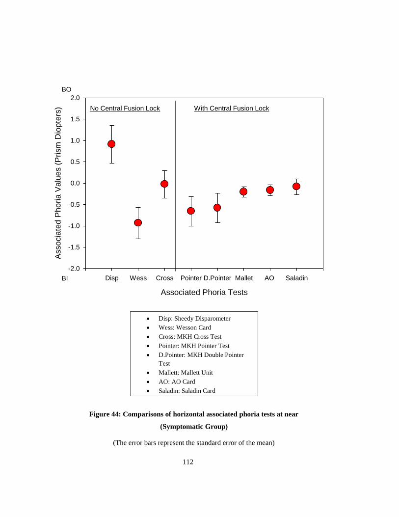
112
Associated Phoria Tests
Disp Wess Cross Pointer D.Pointer Mallet AO Saladin
Asso
cia
ted
Ph
oria
Va
lue
s (
Prism
Dio
pte
rs)
-2.0
-1.5
-1.0
-0.5
0.0
0.5
1.0
1.5
2.0
No Central Fusion Lock With Central Fusion Lock
BO
BI
Figure 44: Comparisons of horizontal associated phoria tests at near
(Symptomatic Group)
(The error bars represent the standard error of the mean)
Disp: Sheedy Disparometer
Wess: Wesson Card
Cross: MKH Cross Test
Pointer: MKH Pointer Test
D.Pointer: MKH Double Pointer
Test
Mallett: Mallett Unit
AO: AO Card
Saladin: Saladin Card

113
Associated Phoria Tests
Disp Wess Cross Pointer D.Pointer Mallet AO Saladin
Asso
cia
ted
Ph
oria
Va
lue
s (
Prism
Dio
pte
r)
-2.0
-1.5
-1.0
-0.5
0.0
0.5
1.0
1.5
2.0
No Central Fusion Lock With Central Fusion Lock
BO
BI
Figure 45: Comparisons of horizontal associated phoria tests at near
(Asymptomatic Group)
(The error bars represent the standard error of the mean)
Disp: Sheedy Disparometer
Wess: Wesson Card
Cross: MKH Cross Test
Pointer: MKH Pointer Test
D.Pointer: MKH Double Pointer
Test
Mallett: Mallett Unit
AO: AO Card
Saladin: Saladin Card

114
6.6.1.3 Comparison of vertical associated phoria tests at distance and near:
Repeated Measures ANOVA of vertical associated phoria tests at both distance and near did not
show any significant differences among different tests. In addition, the analysis did not reveal any
significant difference between subject groups or significant subject by test interaction. Figure 46
shows the distance test data for symptomatic group where the variation between the means was the
largest. At near, the mean range was very small (from 0.008 BU to 0.008 BD ).

115
Associated Phoria Tests
Cross D.Pointer Rectangle Mallet AO
Associa
ted P
horia V
alu
es (
Prism
Dio
pte
r)
-1.00
-0.75
-0.50
-0.25
0.00
0.25
0.50
0.75
1.00
No CentralFusion Lock
With Central Fusion Lock
BU(RE)
BD(RE)
Figure 46: Comparisons of vertical associated phoria tests at distance
(Symptomatic Group)
(The error bars represent the standard error of the mean)
Cross: MKH Cross Test
D.Pointer: MKH Double
Pointer Test
Rectangle: MKH Rectangle
Test
Mallett: Mallett Test
AO: AO Slide

116
6.6.2 Discussion:
To my knowledge, no comparison study between the MKH-Haase charts and other associated
phoria charts in the English literature has been done. For the distance horizontal associated phoria
tests, the results were similar in both groups. The difference in the means was no greater than 0.25 Δ
and so it is unlikely that this difference would be clinically important. MKH-Haase targets with
central fusion locks had distance associated phoria values that were comparable to the Mallett Test
and AO Distance Slide. Our results showing there is no significant difference between values of
Mallett Test and AO Vectographic Slide at distance was consistent with the Brownlee and Goss
findings (1988). However, the MKH-Haase charts were more variable especially for the symptomatic
group. That might give an advantage for the Pointer and Double Pointer Tests to measure horizontal
associated phoria at distance more accurately than the Mallett Test and AO slides.
Tests with central fusion locks results were slightly more eso values than the test without a central
fusion lock. The closest explanation for more base-in values with the Cross Test was probably the
lack of a central fusion lock. Ukwade (2000) found that fixation disparity with a central fusion lock,
or with central and peripheral fusion locks, were lower than with peripheral fusion lock only.
Wildsoet & Cameron (1985) cited that previous studies e.g. “(Jampolsky (quoted in Lyons, 1966),
Hebbard (1960), Carter (1964), Lyons (1966), Ogle (1967), Grolman (1971) and Rutstein (1977)”
have shown that fixation disparity magnitude has been changed after presenting foveal fusion locks.
Most of those studies have shown that fixation disparity reduced with foveal fusion lock. For
example, Carter (1964b; 1980) measured fixation disparity with and without central fusion lock at 4.3
meter distance from the subjects. He found that the magnitude of fixation disparity for the majority of
his subjects was always higher and more eso when there is no central fusion lock. However, the
change in the magnitude of X- intercepts (associated phoria) after presenting the foveal fusion lock
was not similar with all of his subjects. These differences in associated phoria values between

117
different subjects were due to different types of fixation disparity curve. Ogle’s data (1967) shows
fixation disparity decreased and shifted toward the exo direction as the fusion locks become more
central which is consistent with Carter’s finding. However, the associated phoria values did not
change significantly even though there was a small eso shift as the fusion locks become more central.
The Wildsoet & Cameron (1985) findings contradict Carter’s (1964b) findings. Their results showed
that fixation disparity and associated phoria were higher and shifted toward eso when a central fusion
lock was inserted using the Sheedy Disparometer at 40 cm viewing distance.
Although there were differences between the symptomatic and asymptomatic subjects across the
various horizontal associated phoria tests at near, these differences were generally related to the
magnitude of any differences across tests between the two groups. Regardless of the subject category,
the Sheedy Disparometer mean values was more eso than all other tests and the Wesson Card mean
value was more exo compared with all other tests. As a result, the difference between the
Disparometer and Wesson Card was approximately 2.0 . The Cross Test was shifted toward more
base-out than tests with a central fusion lock at near.
The large difference between the Sheedy Disparometer and Wesson Card with other tests is likely
due to the target design. First neither the Sheedy Disparometer nor Wesson Card has a central fusion
lock. In addition, the monocular lines of the Sheedy Disparometer are located behind the rest of the
plane of fixation. If the subject had no fixation disparity at the fixation plane, then the nonius lines
that were in physical alignment, but located behind the fixation plane, would appear as an eso fixation
disparity. That could be the possible reason for the higher base-out associated phoria values with this
test (Wildsoet & Cameron, 1985).
Previous comparisons studies between common clinical tests, that do not include MKH-Haase
charts, showed similar results to our study (Van Haeringen et al., 1986; Brownlee & Goss, 1988;
Goss & Patel, 1995; Ngan et al., 2005; Frantz et al., 2011). The one exception was the Mallett Unit

118
and Sheedy Disparometer comparison done by Pickwell et al. (1988) which showed that the mean
associated phoria values measured with the Disparometer was higher in magnitude and shifted more
toward base in direction than the Mallett Unit.
Comparisons of vertical associated phoria of MKH-Haase charts and other common clinical tests
did not show any significant differences at both distance and near. This result was expected since the
natural status of the vertical vergence system is less variable and the majority of the subjects had a
vertical associated phoria no greater than 0.25 The mean values of vertical associated phoria tests
varied from zero prism dioptre to 0.12 .
The 95% limits of agreement according to the Bland and Altman method of repeatability (Bland
& Altman 1986, 1995) were calculated for associated phoria tests when the differences between them
were not significant. Tables 29 to 32 show the 95% limits of agreement between different horizontal
and vertical associated phoria tests at both distance and near respectively. Associated phoria values
were rounded to the closest 0.25 step in most of cases, or to the closest 1/8 step in other cases.
Table 29: 95% limits of agreement for different horizontal associated phoria tests at distance
Test Double Pointer Test Mallett Unit AO Slide
Pointer Test -0.75 to 0.50 *
-0.37 to 0.37 ^
-1.50 to 1.86 *
-0.75 to 1.00 ^
-1.50 to 1.86 *
-0.87 to 1.00 ^
Double Pointer Test -0.62 to 1.25 *
-1.00 to 1.00 ^
-0.62 to 1.25 *
-1.00 to 1.00 ^
Mallett Unit -0.50 to 0.50 *
-0.25 to 0.25 ^
(*)Symptomatic Group, (^) Asymptomatic Group

119
Table 30: 95% limits of agreement for different vertical associated phoria tests at distance
Test Double Pointer
Test Rectangle Test Mallett Unit AO Slide
Cross Test -0.25 to 0.12 *
-0.12 to 012 ^
-0.25 to 0.12 *
-0.12 to 012 ^
-0.25 to 0.12 *
-0.12 to 012 ^
-0.25 to 0.12 *
-0.12 to 012 ^
Double Pointer
Test
-0.25 to 0.12 *
-0.25 to 0.25 ^
-0.25 to 0.12 *
-0.12 to 012 ^
-0.25 to 0.12 *
-0.12 to 012 ^
Rectangle Test -0.25 to 0.12 *
-0.12 to 012 ^
-0.25 to 0.12 *
-0.12 to 012 ^
Mallett Unit -0.25 to 0.12 *
0 ^ (*)Symptomatic Group, (^) Asymptomatic Group
Table 31: 95% limits of agreement for different horizontal associated phoria tests at near
Test Mallett Unit AO
Card
Saladin
Card
Double
Pointer
-3.00 to 2.25 *
-1.25. to 0.75 ^
-3.00 to 2.25 *
-1.25. to 0.75 ^
3.00 to 2.50 *
-1.25. to 1.00 ^
Mallett
Unit
-0.50 to 0.50 *
-0.25 to 0.25 ^
-0.75 to 0.50 *
-0.25 to 0.50 ^
AO
Card
-0.75 to 0.50 *
-0.25 to 0.50 ^ (*)Symptomatic Group, (^) Asymptomatic Group
Table 32: 95% limit of agreement for different vertical associated phoria tests at near
Test Wesson
Card
Cross
Test
Rectangle
Test
Mallett
Unit
AO
Card
Saladin
Card
Sheedy
Disparometer -0.25 to 0.12 *
-0.12 to 012 ^
0 *
0 ^
-0.25 to 0.12 *
-0.12 to 012 ^
0 *
0 ^
0 *
0 ^
0 *
0 ^
Wesson
Card
-0.25 to 0.12 * -0.25 to 0.25 ^
-0.25 to 0.12 * -0.12 to 012 ^
-0.25 to 0.12 * -0.12 to 012 ^
-0.25 to 0.12 * -0.12 to 012 ^
-0.25 to 0.12 * -0.12 to 012 ^
Cross
Test
-0.25 to 0.12 *
-0.12 to 012 ^
0 *
0 ^
0 *
0 ^
0 *
0 ^
Rectangle
Test
-0.25 to 0.12 *
-0.12 to 012 ^
-0.25 to 0.12 *
-0.12 to 012 ^
-0.25 to 0.12 *
-0.12 to 012 ^
Mallett
Unit
0 *
0 ^
0 *
0 ^
AO
Card
0 *
0 ^
(*)Symptomatic Group, (^) Asymptomatic Group

120
6.7 Comparison of MKH-Haase stereoacuity charts with other common stereoacuity
tests:
The results of three different distance stereoacuity tests (Line Test, Step Test, and AO
Vectographic Slide) were compared for the crossed disparities. The results from six near stereoacuity
tests (Line Test, Step Test, AO Cards, Randot Circles Test, Random dot Randot Test, and TNO Test)
were also examined. Only the values for the crossed disparities of MKH-Haase tests were used
because the other tests’ protocols did not recommend measuring stereoacuity with two different
disparities.
For each test, the mean and standard deviation were calculated; however, because the minimum
disparity and step size varies across tests, the number of subjects who attained the minimum
stereothreshold of the test, the number of subjects who attained 60 sec of arc or better, and number of
subjects who failed to distinguish the maximum stereothreshold of the test were determined.
Statistical analysis across tests was carried out using the Chi-square test based on the number of
subjects who attained 60 sec of arc or better with a 0.05 rejection level.
6.7.1 Results:
6.7.1.1 Comparison of stereoacuity tests at distance:
Thirty-four symptomatic participants and 40 asymptomatic participants (aged range 18 -36 years
old) participated in this study. Table 33, Figure 47, and Figure 48 summarize the results of different
criteria measurements of stereoacuity tests at distance for both groups. The results of the Line Test at
distance showed that it is possible to create a distance stereotest that can evaluate down to 10 sec arc
and approximately 30% of the young adults could perceive it. As expected, the Step Test, which is a
random dot test, was more difficult based on the lower number of subjects in the 60 sec arc or better
category and the lower number of subjects who were unable to identify the maximum stereothreshold.
Although the AO distance stereotest only measures down to 60 sec arc, its disparities appear to be
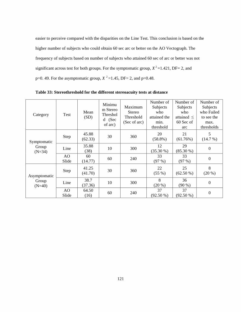
121
easier to perceive compared with the disparities on the Line Test. This conclusion is based on the
higher number of subjects who could obtain 60 sec arc or better on the AO Vectograph. The
frequency of subjects based on number of subjects who attained 60 sec of arc or better was not
significant across test for both groups. For the symptomatic group, X 2
=1.421, DF= 2, and
p=0. 49. For the asymptomatic group, X 2
=1.45, DF= 2, and p=0.48.
Table 33: Stereothreshold for the different stereoacuity tests at distance
Category Test Mean
(SD)
Minimu
m Stereo
Threshol
d (Sec
of arc)
Maximum
Stereo
Threshold
(Sec of arc)
Number of
Subjects
who
attained the
min.
threshold
Number of
Subjects
who
attained ≤
60 Sec of
arc
Number of
Subjects
who Failed
to see the
max.
thresholds
Symptomatic
Group
(N=34)
Step 45.88
(62.33) 30 360
20
(58.8%)
21
(61.76%)
5
(14.7 %)
Line 35.88
(38) 10 300
12
(35.30 %)
29
(85.30 %) 0
AO
Slide
60
(14.77) 60 240
33
(97 %)
33
(97 %) 0
Asymptomatic
Group
(N=40)
Step 41.25
(41.70) 30 360
22
(55 %)
25
(62.50 %)
8
(20 %)
Line 38.7
(37.36) 10 300
8
(20 %)
36
(90 %) 0
AO
Slide
64.50
(16) 60 240
37
(92.50 %)
37
(92.50 %) 0

122
Figure 47: Comparisons of stereoacuity tests at distance
(Symptomatic Group)
Stereoacuity Tests
Step Line AO Slide
Fre
quency o
f S
ubje
cts
(%
)
0
10
20
30
40
50
60
70
80
90
100
Frequency who obtained the minimum disparity
Frequency who obtained 60 sec of arc or better
Frequency who failed to see the maximum disparity

123
Figure 48: Comparisons of stereoacuity tests at distance
(Asymptomatic Group)
Stereoacuity Tests
Step Line AO Slide
Fre
quency o
f S
ubje
cts
(%
)
0
10
20
30
40
50
60
70
80
90
100
Frequency who obtained the minimum disparity
Frequency who obtained 60 sec of arc or better
Frequency who failed to see the maximum disparity

124
6.7.1.2 Comparison of stereoacuity tests at near:
The same subjects also participated in the near stereotest evaluation. Because the minimum
stereothreshold of Random Dot Randot Test was very high (250 second of arc), all participants were
able to identify it. For this reason, this test was excluded from further comparison. Table 34 and
Figure 45 summarize the results for the different measurement criteria. The results for the near Line
Test showed that it is possible to create a near stereotest that can evaluate down to 10 sec arc and
approximately 90% of the young adults could perceive it. Again, the random dot Step and the TNO
tests were more difficult based on the number of subjects who could identify stereoacuity of 60
second of arc or better and the number of subjects who could not identify the maximum
stereothreshold. Based on the criterion of a stereoacuity of at least 60 sec arc, the local stereotests
were equivalents. All but one subject could perceive this disparity in all local stereotests. The one
exception was in the asymptomatic group and could not obtain 60 sec arc on the Randot Circle Test.
In terms of the random dot tests, more subjects were able to obtain a stereothreshold of at least 60
second of arc on the Step Test compared with the TNO Test. The Chi-square test did not show any
significant differences between the frequencies of subjects who could obtain at least 60 sec arc for the
different stereotests at near. For the symptomatic group, X 2
=0.62, DF= 4, and p=0.96. For the
asymptomatic group, X 2
=1.2, DF= 4, and p= 0.86.

125
Table 34: Stereothreshold of different stereoacuity tests at near
Category Test
Mean
(SD)
Minimum
Stereo
Threshold
Maximum
Stereo
Threshold
Number
of
Subjects
the min.
threshold
Number
of
Subjects
who
attained ≤
60”
Number of
Subjects
who Failed
to see the
maxi
thresholds
Symptomatic
Group
(N=34)
TNO 65.73
(63.74) 15 480
9
(26.47 %)
27
(79.4 %) 0
Step 30.88
(13) 30 360
30
(88.20 %)
31
(91.18 %)
2
(5.8 %)
Line 11.17
(3.27) 10 300
30
(88.20 %)
34
(100 %) 0
AO Card 17
(10.59) 12 600
27
(79.4 %)
34
(100 %) 0
Randot
Circles
21
(2.95) 20 400
30
(88.20 %)
34
(100 %) 0
Asymptomatic
Group
(N=40)
TNO 66
(56) 15 480
10
(25 %)
29
(72.50 %) 0
Step 41.25
(52.9) 30 360
36
(90 %)
38
(95 %) 0
Line 11.25
(7.9) 10 300
39
(97 %)
40
(100 %) 0
AO Card 16.4
(8.6) 12 600
31
(77.50 %)
40
(100 %) 0
Randot
Circles
21.50
(7.95) 20 400
37
(92.50 %)
39
(97 %) 0

126
Figure 49: Comparisons of stereoacuity tests at near
(Symptomatic group)
Stereoacuity Tests
TNO Step Line AO Card Randot Circles
Fre
quency o
f S
ubje
cts
(%
)
0
10
20
30
40
50
60
70
80
90
100
110
Frequency who obtained the minimum disparity
Frequency who obtained 60 sec of arc or better
Frequency who failed to see the maximum dispari
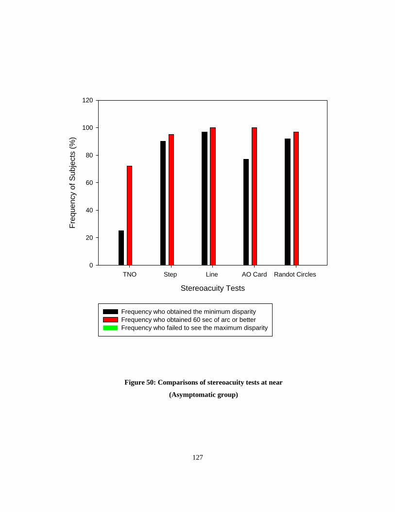
127
Figure 50: Comparisons of stereoacuity tests at near
(Asymptomatic group)
Stereoacuity Tests
TNO Step Line AO Card Randot Circles
Fre
quency o
f S
ubje
cts
(%
)
0
20
40
60
80
100
120
Frequency who obtained the minimum disparity
Frequency who obtained 60 sec of arc or better
Frequency who failed to see the maximum disparity

128
6.7.2 Discussion:
Because different clinical stereoacuity tests vary with their designs, it is difficult to compare the
means threshold values or even the percentage of subjects who could obtain the minimum threshold
possible on the test, because this value varied across tests. Instead, I examined the percentage of
subjects who could obtain at least 60 sec arc acuity at either distance or near. The reason for selecting
this value was that most of stereotests present this disparity.
The MKH-Haase system demonstrated that it was possible to measure clinically stereoacuity as
low as 10 seconds of arc at distance and near. Around 30% of participants could identify the
minimum stereothreshold of the MKH-Haase contour Line Test at distance and around 90% at near.
The AO Card at near can measure down to 12 sec but less than 80 % of participants could identify the
minimum stereothreshold .
Stereothreshold results at near showed that almost all of the subjects had the minimum
stereothreshold when measured with different contour stereotests. The Line Test had the higher
number of subjects for both groups followed by the Random Dot Circles Test, and then the AO Card.
The minimum stereothreshold among contour tests can be measured with the Line Test. The Line
Test can measure stereothreshold down to 10 seconds of arc. AO Card can measure to 12 seconds of
arc, and RDC to 20 seconds of arc. This finding gives an advantage of MKH-Haase Line Test among
other clinical stereotests to measure contour stereoacuity at near. All subjects except one had 60
seconds of arc or better when measured with those contour tests and nobody failed to see the
maximum stereothreshold.
Results of random dot tests at near showed that the Randot Test had the highest number of subjects
who achieved the minimum stereothreshold among other tests. This finding was not surprising since
the minimum stereothreshold with this test is very high (250 second of arc). The TNO Test had a
lower number of participants for those who had minimum stereothreshold and for those who had 60

129
second of arc or better in comparison with MKH-Haase Step Test. Nobody failed to see the maximum
stereothreshold with TNO Test (480 second of arc). However, only two participants from the
symptomatic group failed to distinguish the maximum stereothreshold of the MKH-Haase Step Test
(360 second of arc). Since the number of subjects who could identify 60 second of arc or better was
higher with the Step Test than the TNO test, we may consider the Step Test as a preferable random
dot stereotest at near. One reason may be that the retinal luminance is higher for the Step Test because
the Polariods transmit more light relative to the red/green spectacles required to perform the TNO
test. However, the differences in the frequencies of subjects between TNO and Step Test were not
significant.
Comparison between symptomatic and asymptomatic groups showed that for most of the
stereoacuity tests at distance and near the number of participants who met our criteria was either
higher with the asymptomatic group, or the difference was very small. This finding suggests that
stereoacuity may not be reduced in patients with symptoms suggestive of binocular vision problems.
If we consider fixation disparity as an indication of presence or absence of visual stress, previous
studies showed different findings about how stereoacuity is dependent on fixation disparity and visual
stress. Manan, et al. (2001) measured stereoacuity with the TNO Test for asymptomatic people
without fixation disparity and with symptomatic people who had fixation disparity. They found there
was a significant difference in stereoacuity measurements between the two groups. Induced
heterophoria of small prismatic power (±2 ) did not affect the measurements of stereoacuity when
measured by the Howard-Dolman test at distance of 6 meters. However, stereoacuity was affected
when the amount of induced phoria was increased (Heravian et al., 2012). Kromeier, M et al. (2003),
showed that stereoacuity measured with Freiburg Test decreased under prismatic stress. However, the
correlation between fixation disparity and stereoacuity under prismatic stress was very low. Saladin

130
(1995) found that there is not an effect of induced exophoria on stereoacuity. However, induced
esophoria has an effect of stereoacuity.
My results suggest that using only stereoacuity tests to screen for nonstrabismic binocular
dysfunction in a symptomatic adult population may not be of any value when the acuity is equal in
each eye. Further comparison using subjects with binocular dysfunctions like strabismus and
amblyopia may be necessary in order to determine which stereotests have a higher clinical value.

131
Chapter 7
Summary and Conclusions
1) Results of within and between-session repeatability of different MKH-Haase associated phoria
charts can be summarized to the following points:
a) Most of the horizontal and vertical MKH-Haase associated phoria charts showed no significant
differences between View 1 and View 2 at distance or the difference was very small. There was a
strong linear correlation between View 1 and View 2 charts with slopes statistically identical to 1.0
and the y-intercept statistically identical to zero. However, there were some cases where the values
measured within View 1 and View 2 differed slightly. The exact reason for these slight differences is
uncertain, but it could be related to the angle between the display and the patient’s line sight.
b) All of the horizontal and vertical associated phoria charts at near showed no significant differences
and strong correlations between View 1 and View 2 charts. However, the regression’s slope was
greater than 1.0 with vertical associated phoria of Cross Test for the symptomatic group of the first
session. This is because the values of View 2 were on average higher than View 1. The linear
regression’s slope for the vertical Double Pointer Test for the symptomatic group at the second
session was less than 1.0. This was a result of larger vertical phorias measured in View 1 being
reduced in View 2.
c) Comparison between Session 1 and Session 2 results did not reveal significant differences between
means of the two sessions at both distance and near for all of associated phoria tests. The correlations
between the two sessions with the majority of horizontal tests were high and significant. However, the
correlations between vertical associated phoria tests were low and non-significant with the majority of
the tests. This was because nearly all of subjects had identical vertical associated phoria values except
few subjects had large (0.50 ) differences between the two views.

132
2) Results of within and between-session repeatability of different MKH-Haase associated
stereoacuity tests can be summarized to the following points:
a) Stereoacuity measured with crossed disparity charts were marginally higher than uncrossed
disparity charts with most of stereoacuity tests at both distance and near.
b) Although the mean stereoacuity for crossed disparities were higher, the differences for the majority
tests were not significant. The differences were statistically significant at the first session for the
symptomatic group’s Line Test and asymptomatic group's Step Test. For the second session at
distance, the differences were significant with Step Test for both groups. None of tests for both
sessions at near had significant differences between the two disparities.
c) Correlation between crossed and uncrossed disparities was either high or moderate with most of the
tests at both distance and near for both sessions. The slope was less than 1.0 with the Line Test and
Step Test at distance though. This was because the Stereoacuity in the first session was on average
better than the second session for those tests. The correlation between crossed and uncrossed
disparities of the Line Test was higher than the Step Test.
d) The differences between sessions for both disparities were not significant for most of the tests. The
symptomatic group’s Step Test crossed disparity and asymptomatic group's Step Test uncrossed
disparity were exceptions. The correlation between sessions for the crossed disparity tests at distance
was good and significant except for the Line Test of the asymptomatic group. With uncrossed
disparity charts, the correlation was high and significant for only the symptomatic subjects’ Line Test
results. Correlations between the two sessions at near were either low or non-significant in the
majority of stereotests for both disparities. The exception was the crossed disparity charts for the
asymptomatic group.
e) The Hand test requires subjects to identify a hand form that appears in depth. Large numbers of
participants from both groups could not identify this shape at the first session. The number of

133
subjects who saw the form at the second session increased in both groups. This result indicates that
there is a learning/practice effect with this test.
3) None of the subjects showed any noticeable stereo delay with the Stereo Triangle Test at either
distance or near. This suggests that the stereo delay test may not be a useful test in assessing
nonstrabismic binocular vision disorders.
4) Subjects’ behaviors with Stereo Balance Test were variable for the two views and across sessions.
Within and between-session repeatability of ocular prevalence tests showed that there were
significant differences between sessions or subject groups. Only 20 % of the symptomatic group’s
subjects and 40% of asymptomatic group’s subjects showed the same ocular prevalence result within
and across sessions at distance. Only 30 % of the symptomatic group’s subjects and 67% of
asymptomatic group’s subjects showed the same ocular prevalence result within and across sessions
at near.
5) Comparison of different associated phoria tests can be summarized to the following points:
a) At distance, the test without a central fusion lock resulted in more exo values than all other tests
with central fusion lock. However, the amount in most of cases was very small (e.g. less than 0.25 ).
Vertical associated phoria tests did not show any significant differences.
b) At near, tests without central fusion lock, except Wesson Card, were more eso than all other tests
with central fusion lock. The Sheedy Disparometer produced the most eso mean value and the
Wesson Card mean value was the most exo. The difference between the Sheedy Disparometer and
Wesson Card mean values was approximately 2 The differences between all other tests were less
than 0.50 . Vertical associated phoria tests did not show any significant differences between tests.
6) Comparison of different stereoacuity tests can be summarized to the following points:
a) At distance, MKH-Haase Line Test can measure contour stereoacuity down to 10 second of arc.
However, contour stereoacuity at distance was easier to perceive with the AO slide based on the

134
number of subjects who attained 60 sec of arc or better on the various contour stereopsis tests. The
MKH- Haase Step Test can be used to measure random dot stereoacuity at distance down to 30 sec of
arc.
b) At near, the MKH-Haase Line Test can measure contour stereoacuity down to 10 second of arc.
The Line Test appeared to be the easiest based on the number of subjects who attained 60 sec of arc
or better. The Random dot Step Test was easier than the TNO Test to measure global stereoacuity at
near. One reason may be that the retinal luminance is higher for the Step Test because the Polaroids
transmit more light relative to the red/green spectacles required to perform the TNO test.
The conclusive statements can be reached about MKH-Haase binocular vision charts according to
the results of this project are first the MKH-Haase charts are considered reliable and repeatable to
measure horizontal and vertical associated phoria at distance and near. Second, the Line Test and Step
Test of the MKH-Haase charts are considered reliable and repeatable to measure fine local and global
stereothreshold at both distance and near. Third, the concept of measuring and correcting long
standing fixation disparity according to the MKH-Haase method by using the Stereo Triangle and
Stereo Balance Tests has not been proven and still questionable. Further researches may be necessary
to validate the ability of Stereo Triangle and Stereo Balance Tests to detect and correct fixation
disparity.

135
Copyright Permissions
Confirmation Number: 11104718
Order Detail ID: 63834388
Strabismus by TAYLOR & FRANCIS THE NETHERLANDS. Reproduced with permission
of TAYLOR & FRANCIS THE NETHERLANDS in the format republish in a
thesis/dissertation via Copyright Clearance Center.

136
Bibliography
Ames Jr, A., & Ogle, K. N. (1932). Size and shape of ocular images: III. Visual sensitivity to
differences in the relative size of the ocular images of the two eyes. Archives of Ophthalmology,
7(6), 904.
Bland, J.M. , & Altman, D. (1986). Statistical methods for assessing agreement between two methods
of clinical measurement. The Lancet, 327(8476), 307-310. doi:http://dx.doi.org/10.1016/S0140-
6736(86)90837-8
Bland, J. M., & Altman, D. G. (1995). Comparing methods of measurement: Why plotting difference
against standard method is misleading. The Lancet, 346(8982), 1085-1087.
doi:http://dx.doi.org/10.1016/S0140-6736(95)91748-9
Brautaset, R. L., & Jennings, J. A. M. (2001). Associated phoria and the measuring and correcting
methodology after H.-J. Haase (MKH). Strabismus, 9(3), 165-176.
doi:10.1076/stra.9.3.165.6764
Brownlee, G. A., & Goss, D. A. (1988). Comparisons of commercially available devices for the
measurement of fixation disparity and associated phorias. Journal of the American Optometric
Association, 59(6), 451-460.
Carter, D. B. (1957). Studies of fixation disparity; historical review. American Journal of Optometry
and Archives of American Academy of Optometry, 34(6), 320-329.
Carter, D. B. (1964a). Fixation disparity with and without foveal fusion contours. American Journal
of Optometry and Archives of American Academy of Optometry, 41, 729-736.
Carter, D. B. (1964b). Fixation disparity with and without foveal fusion contours. American Journal
of Optometry and Archives of American Academy of Optometry, 41, 729-736.
Carter, D. B. (1980). Parameters of fixation disparity. American Journal of Optometry and
Physiological Optics, 57(9), 610-617.

137
Corbett, A., & Maples, W. C. (2004). Test-retest reliability of the Saladin card. Optometry, 75(10),
629-639.
Eskridge, J. B. (1991). In Amos J. F., Bartlett J. D. (Eds.), Clinical procedures in optometry.
Philadelphia: Philadelphia: J.B. Lippincott.
Frantz, K. A., Elston, P., Michalik, E., Templeman, C. D., & Zoltoski, R. K. (2011). Comparison of
fixation disparity measured by Saladin card and Disparometer. Optometry and Vision Science,
88(6), E733-E741.
Gerling, J., Ball, M., Bömer, T., Bach, M., & Kommerell, G. (1998). Fixation disparity in the Zeiss
Pola-Zeigertest (clock hand test): Not representative for eye position under natural viewing
conditions. [Fixationsdisparation am Pola-Zeigertest: Nicht reprasentativ fur die augenstellung
unter naturlichen sehbedingungen] Klinische Monatsblatter Fur Augenheilkunde, 212(4), 226-
233.
Gerling, J., De Paz, H., Schroth, V., Bach, M., & Kommerell, G. (2000). Can fixation disparity be
detected by the 'measuring and correction methods of H.-J. Haase'? [Ist die feststellung einer
fixationsdisparation mit der mess- und korrektionsmethodik nach H.-J. Haase (MKH)
verlasslich?] Klinische Monatsblatter Fur Augenheilkunde, 216(6), 401-411.
Goss, D. A., & Patel, J. (1995). Comparison of fixation disparity curve variables measured with the
Sheedy Disparometer and the Wesson fixation disparity card. Optometry and Vision Science,
72(8), 580-588.
Grabowska, A. (1983). Lateral differences in the detection of stereoscopic depth. Neuropsychologia,
21(3), 249-257.
Haase, H. (1962). Binocular testing and distance correction with the berlin POLATEST, journal of
the american optometric association .34(2), 115-124.

138
Hall, C. (1982). The relationship between clinical stereotests. Ophthalmic and Physiological Optics,
2(2), 135-143.
Harris, L. R. & Jenkin, M. R. M. (2011). Vision in 3D Environment. Cambridge University Press:
New York.
Heravian, J., Hosein, S., Yazdi, A., Baghebani, F., Mahjoob, M., Ostadimoghaddam, H., Yekta, A.,
Azimi, A (2012). Effect of induced heterophoria on distance stereoacuity by using the Howard-
Dolman test. Iranian Journal of Ophthalmology, 24(1):25-30.
Hofstetter, H. W. (2000). Dictionary of visual science and related clinical terms (Vol. 1).
Butterworth-Heinemann Medical.
Howard, H. J. (1919). A test for the judgment of distance. Transactions of the American
Ophthalmological Society, 17, 195.
Howard, I. P. (2002). Seeing in depth, volume 1: Basic mechanisms. Ontario, Canada: I.Porteous,
Howard, I. P. (2008). In Rogers B. J. (Ed.), Seeing in depth. New York ; Oxford: Oxford University
Press.
Julesz, B. (1960). Binocular depth perception of computer-generated patterns. Bell System Technical
Journal; Bell System Technical Journal,
Kommerell, G., Schmitt, C., Kromeier, M., & Bach, M. (2003). Ocular prevalence versus ocular
dominance. Vision Research, 43(12), 1397-1403.
Kommerell, G., Gerling, J., Ball, M., De Paz, H., & Bach, M. (2000). Heterophoria and fixation
disparity: A review. Strabismus, 8(2), 127-134.
Kromeier, M., Schmitt, C., Bach, M., & Kommerell, G. (2003). Stereoacuity versus fixation disparity
as indicators for vergence accuracy under prismatic stress. Ophthalmic and Physiological Optics,
23(1), 43-49.
139
Kromeier, M., Schmitt, C., Bach, M., & Kommerell, G. (2002a). Do prisms according to hans-
joachim haase improve stereoacuity? [Bessern Prismen nach Hans-Joachim Haase die
Stereosehscharfe?] Klinische Monatsblatter Fur Augenheilkunde, 219(6), 422-428.
doi:10.1055/s-2002-32883
Kromeier, M., Schmitt, C., Bach, M., & Kommerell, G. (2002b). Do prisms according to hans-
joachim haase influence ocular prevalence? [Beeinflussen Prismen nach Hans-Joachim Haase
die Augenpravalenz?] Klinische Monatsblatter Fur Augenheilkunde, 219(12), 851-857.
doi:10.1055/s-2002-36951
Landers, D. D., & Cormack, L. K. (1997). Asymmetries and errors in perception of depth from
disparity suggest a multicomponent model of disparity processing. Perception & Psychophysics,
59(2), 219-231.
LARSON, W. L. (1990). An investigation of the difference in stereoacuity between crossed and
uncrossed disparities using Frisby and TNO tests. Optometry & Vision Science, 67(3), 157-161.
Larson, W. (1985). Does the howard-dolman really measure stereoacuity? American Journal of
Optometry and Physiological Optics, 62(11), 763-767.
Lie, I., & Opheim, A. (1985). Long-term acceptance of prisms by heterophorics. Journal of the
American Optometric Association, 56(4), 272-278.
Lie, I., & Opheim, A. (1990). Long-term stability of prism correction of heterophorics and
heterotropics; a 5 year follow-up. part I: Heterophorics. Journal of the American Optometric
Association, 61(6), 491-498.
London, R., & Crelier, R. S. (2006). Fixation disparity analysis: Sensory and motor approaches.
Optometry - Journal of the American Optometric Association, 77(12), 590-608.

140
London, R. F., & Wick, B. (1987). Vertical fixation disparity correction: Effect on the horizontal
forced-vergence fixation disparity curve. American Journal of Optometry and Physiological
Optics, 64(9), 653-656.
Mallettt, R. (1974). Fixation disparity-its genesis and relation to asthenopia. Ophthalmic Optician, 14,
1159-1168.
Manan, F. A., Jenkins, T., & Collinge, A. (2001). The effect of clinical visual stress on stereoacuity
measured with the TNO test. The Malaysian Journal of Medical Sciences: MJMS, 8(2), 25.
Mitchell, D. E. (1966a). Retinal disparity and diplopia. Vision Research, 6(7), 441-451.
Mitchell, D. E. (1966b). A review of the concept of "panum's fusional areas". American Journal of
Optometry and Archives of American Academy of Optometry, 43(6), 387-401.
Nelson, J. (1988). Binocular vision: Disparity detection and anomalous correspondence. Textbook of
Optometry, , 217-237.
Ngan, J., Goss, D. A., & Despirito, J. (2005). Comparison of fixation disparity curve parameters
obtained with the Wesson and Saladin fixation disparity cards. Optometry and Vision Science,
82(1), 69-74.
Ogle, K. N., & deH PRANGEN, A. (1953). Observations on vertical divergences and hyperphorias.
Archives of Ophthalmology, 49(3), 313.
Ogle, K. N. (1958). Fixation disparity and oculomotor imbalance. The American Orthoptic Journal,
8, 21-36.
Ogle, K. N., Mussey, F., & Prangen, A. D. (1949). Fixation disparity and the fusional processes in
binocular single vision. American Journal of Ophthalmology, 32(8), 1069-1087.
Ogle, K. N., Martens, T. G., & Dyer, J. A. (1967). Oculomotor imbalance in binocular vision and
fixation disparity Lea & Febiger Philadelphia.

141
Ogle, K. N., & Prangen, A. d. (1951). Further considerations of fixation disparity and the binocular
fusional processes. American Journal of Ophthalmology, 34(5 PART 2), 57-72.
Ogle, K. N., 1902-, & Ogle, K. N., 1902-.Researches in binocular vision. Philadelphia, W. B.
Saunders, 1950: Philadelphia, W. B. Saunders, 1950.
Palmer, D. (1961). Measurement of the horizontal extent of panum's area by a method of constant
stimuli. Journal of Modern Optics, 8(2), 151-159.
Palmer, E. A., & Von Noorden, G. K. (1978). The relationship between fixation disparity and
heterophoria. American Journal of Ophthalmology, 86(2), 172-176.
Pickwell, L. D., Gilchrist, J. M., & Hesler, J. (1988). Comparison of associated heterophoria
measurements using the Mallettt test for near vision and the Sheedy Disparometer. Ophthalmic
and Physiological Optics, 8(1), 19-25.
Remole, A. (1983). Border enhancement as a function of binocular fixation performance. American
Journal of Optometry and Physiological Optics, 60(7), 567-577.
Remole, A. (1984). Binocular fixation misalignment measured by border enhancement: A simplified
technique. American Journal of Optometry and Physiological Optics, 61(2), 118-124.
Remole, A. (1985). Fixation disparity vs. binocular fixation misalignment. American Journal of
Optometry and Physiological Optics, 62(1), 25-34.
Remole, A., Code, S. M., & Matyas, C. E. (1986). Objective measurement of binocular fixation
misalignment. American Journal of Optometry and Physiological Optics, 63(8), 631-638.
Rowe, F. J. (2004). Clinical orthoptics. Oxford ; Malden, MA: Blackwell Pub.
Rutstein, R. P. (1998). Anomalies of binocular vision : Diagnosis & management. St. Louis, Mo. ;
London: Mosby.
Saladin, J. J., & Carr, L. W. (1983). Fusion lock diameter and the forced vergence fixation disparity
curve. American Journal of Optometry and Physiological Optics, 60(12), 933-943.

142
Saladin, J. (1995). Effects of heterophoria on stereopsis. Optometry and Vision Science, 72(7), 487-
492. doi:10.1097/00006324-199507000-00008
Scheiman, M. (2008). In Wick B. (Ed.), Clinical management of binocular vision : Heterophoric,
accommodative, and eye movement disorders. Philadelphia: Lippincott Williams & Wilkins.
Schor, C. (1980). Fixation disparity: A steady state error of disparity-induced vergence. Am J Optom
Physiol Opt, 57(9), 618-631.
Schor, C. M. (1979a). The influence of rapid prism adaptation upon fixation disparity. Vision
Research, 19(7), 757-765. doi:10.1016/0042-6989(79)90151-2
Schor, C. M. (1979b). The relationship between fusional vergence eye movements and fixation
disparity. Vision Research, 19(12), 1359-1367. doi:10.1016/0042-6989(79)90208-6
Schroth, V. (2012). Binocular correction: Aligning prisms according to the Haase approach. De
Groot Drukkerij, NL: Zijdar Book.
Sheedy, J. E. (1980a). Actual measurement of fixation disparity and its use in diagnosis and
treatment. Journal of the American Optometric Association, 51(12), 1079-1084.
Sheedy, J. E. (1980b). Fixation disparity analysis of oculomotor imbalance. American Journal of
Optometry and Physiological Optics, 57(9), 632-639.
Sheedy, J. E., & Saladin, J. J. (1977). Phoria, vergence, and fixation disparity in oculomotor
problems. American Journal of Optometry and Physiological Optics, 54(7), 474-478.
Sheedy, J. E., & Saladin, J. J. (1978). Association of symptoms with measures of oculomotor
deficiencies. American Journal of Optometry and Physiological Optics, 55(10), 670-676.
Simons, K. (1981). Comparison of the Frisby, random-dot E, TNO, and Randot circles stereotests in
screening and office use. Archives of Ophthalmology, 99(3), 446-452.
Steinman, S. B., 1956. (2000). In Steinman B. A., Garzia R. P. (Eds.), Foundations of binocular
vision: A clinical perspective. New York: McGraw-Hill.

143
Stidwill, D. (2011). In Fletcher R.,FBCO (Ed.), Normal binocular vision : Theory, investigation and
practical aspects. Chichester, West Sussex; Malden, MA: Wiley-Blackwell.
Ukwade, M. T. (2000). Effects of nonius line and fusion lock parameters on fixation disparity.
Optometry & Vision Science, 77(6), 309-320.
Van Haeringen, R., McClurg, P., & Cameron, K. D. (1986). Comparison of Wesson and modified
seedy fixation disparity tests. Do fixation disparity measures relate to normal binocular status?
Ophthalmic and Physiological Optics, 6(4), 397-400.
Verhoeff, F. (1942). Simple quantitative test for acuity and reliability of binocular stereopsis.
Archives of Ophthalmology, 28(6), 1000.
Weymouth, F. W. (1958). Visual sensory units and the minimal angle of resolution. American
Journal of Ophthalmology, 46(1, Part 2), 102.
Wildsoet, C., & Cameron, K. (1985). The effect of illumination and foveal fusion lock on clinical
fixation disparity measurements with the seedy Disparometer. Ophthalmic and Physiological
Optics, 5(2), 171-178.
Wirt, S. (1947). A new near-point stereopsis test. Optom Weekly, 38, 647-649.
Woo, G. C., & Sillanpaa, V. (1979). Absolute stereoscopic thresholds as measured by crossed and
uncrossed disparities. American Journal of Optometry and Physiological Optics, 56(6), 350-355.
Yekta, A. A., & Pickwell, L. D. (1986). The relationship between heterophoria and fixation disparity.
Clinical and Experimental Optometry, 69(6), 228-231.