..........................................................................................................................................................................................................................

SIMULATING WHOLESUPERCOMPUTER APPLICATIONS

..........................................................................................................................................................................................................................

DETAILED SIMULATIONS OF LARGE SCALE MESSAGE-PASSING INTERFACE PARALLEL

APPLICATIONS ARE EXTREMELY TIME CONSUMING AND RESOURCE INTENSIVE. A NEW

METHODOLOGY THAT COMBINES SIGNAL PROCESSING AND DATA MINING TECHNIQUES

PLUS A MULTILEVEL SIMULATION REDUCES THE SIMULATED DATA BY VARIOUS ORDERS OF

MAGNITUDE. THIS REDUCTION MAKES POSSIBLE DETAILED SOFTWARE PERFORMANCE

ANALYSIS AND ACCURATE PERFORMANCE PREDICTIONS IN A REASONABLE TIME.

......The current industrial trend to-ward large multicore processors with multi-ple tens or hundreds of cores poses animportant challenge to research and develop-ment, both for hardware and softwaredesign. To date, researchers and developersdon’t have the right performance evaluationmethods and tools to efficiently design hard-ware and software for large multicore processorsystems. The key enabler to performance eval-uation in today’s computer systems is simula-tion, especially when real hardware is not yetavailable.

Architecture simulation is still sequential,so it depends heavily on the processor’ssingle-thread performance. The advent ofmulticores has signaled the end of individualprocessor speedups and has not benefitedsimulator performance.

Speeding up simulation by parallelizingthe simulator1-3 is complex, and usingFPGA results in specialized simulators.4 Abetter alternative is to reduce the amount ofsimulation performed without losing rele-vance and accuracy. The usual approach to re-duce the amount of simulation is sampling.5,6

That is, the simulator proceeds through theapplication quickly without actually modeling

the hardware, and at certain intervals (ran-dom, or carefully selected), it changes to ahighly detailed (and slow) simulation mode.Statistic analysis of this sampling approachshows that high accuracy can be achievedthrough simulation of small samples. Sam-pling has been widely used in the past to sim-ulate sequential applications running on asingle processor. (For information on otherapproaches to simulation, see the ‘‘RelatedWork in Simulation Tools’’ sidebar.)

However, these sampling methodologiespresent several uncertain aspects when simu-lating parallel systems and applications: howshould the application behave with regard totiming when it’s not being modeled by thesimulator? That is, how should the differentapplication threads and hardware compo-nents align when the next detailed simulationsample is reached?

MethodologyWe used a fine-level characterization of

the application computation, based on signalprocessing and data-mining techniques.Then, we selected what was simulated tominimize the time spent modeling the multi-processor system’s most time-consuming

[3B2-9] mmi2011030032.3d 23/5/011 14:59 Page 32

Juan Gonzalez

Barcelona

Supercomputing Center

Marc Casas

Lawrence Livermore

National Laboratory

Judit Gimenez

Miquel Moreto

Alex Ramirez

Jesus Labarta

Mateo Valero

Polytechnic University

of Catalonia

..............................................................

32 Published by the IEEE Computer Society 0272-1732/11/$26.00 �c 2011 IEEE

components: the processors and the cache hi-erarchy. To do that, we reduced the numberof CPU bursts (the regions between twocommunications in a parallel application)that had to be simulated by selecting thosethat better represented the whole application

execution. After this precise selection, therepresentative set of CPU bursts was a verylow number of the total present in theapplication.

The methodology for accurately selectingthe representative CPU bursts of a parallel

[3B2-9] mmi2011030032.3d 23/5/011 14:59 Page 33

...............................................................................................................................................................................................

Related Work in Simulation Tools

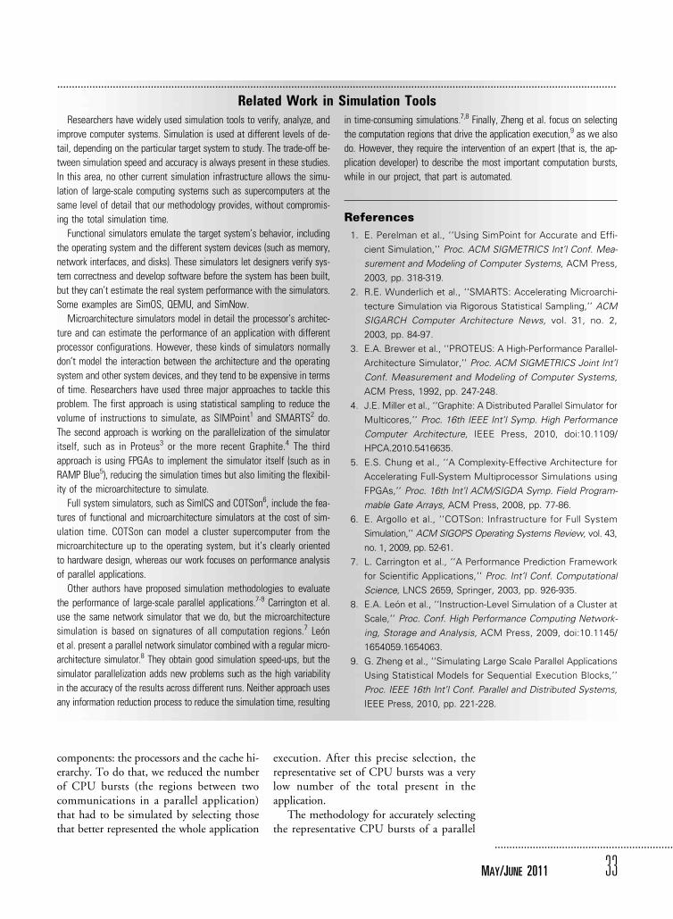
Researchers have widely used simulation tools to verify, analyze, and

improve computer systems. Simulation is used at different levels of de-

tail, depending on the particular target system to study. The trade-off be-

tween simulation speed and accuracy is always present in these studies.

In this area, no other current simulation infrastructure allows the simu-

lation of large-scale computing systems such as supercomputers at the

same level of detail that our methodology provides, without compromis-

ing the total simulation time.

Functional simulators emulate the target system’s behavior, including

the operating system and the different system devices (such as memory,

network interfaces, and disks). These simulators let designers verify sys-

tem correctness and develop software before the system has been built,

but they can’t estimate the real system performance with the simulators.

Some examples are SimOS, QEMU, and SimNow.

Microarchitecture simulators model in detail the processor’s architec-

ture and can estimate the performance of an application with different

processor configurations. However, these kinds of simulators normally

don’t model the interaction between the architecture and the operating

system and other system devices, and they tend to be expensive in terms

of time. Researchers have used three major approaches to tackle this

problem. The first approach is using statistical sampling to reduce the

volume of instructions to simulate, as SIMPoint1 and SMARTS2 do.

The second approach is working on the parallelization of the simulator

itself, such as in Proteus3 or the more recent Graphite.4 The third

approach is using FPGAs to implement the simulator itself (such as in

RAMP Blue5), reducing the simulation times but also limiting the flexibil-

ity of the microarchitecture to simulate.

Full system simulators, such as SimICS and COTSon6, include the fea-

tures of functional and microarchitecture simulators at the cost of sim-

ulation time. COTSon can model a cluster supercomputer from the

microarchitecture up to the operating system, but it’s clearly oriented

to hardware design, whereas our work focuses on performance analysis

of parallel applications.

Other authors have proposed simulation methodologies to evaluate

the performance of large-scale parallel applications.7-9 Carrington et al.

use the same network simulator that we do, but the microarchitecture

simulation is based on signatures of all computation regions.7 Leon

et al. present a parallel network simulator combined with a regular micro-

architecture simulator.8 They obtain good simulation speed-ups, but the

simulator parallelization adds new problems such as the high variability

in the accuracy of the results across different runs. Neither approach uses

any information reduction process to reduce the simulation time, resulting

in time-consuming simulations.7,8 Finally, Zheng et al. focus on selecting

the computation regions that drive the application execution,9 as we also

do. However, they require the intervention of an expert (that is, the ap-

plication developer) to describe the most important computation bursts,

while in our project, that part is automated.

References

1. E. Perelman et al., ‘‘Using SimPoint for Accurate and Effi-

cient Simulation,’’ Proc. ACM SIGMETRICS Int’l Conf. Mea-

surement and Modeling of Computer Systems, ACM Press,

2003, pp. 318-319.

2. R.E. Wunderlich et al., ‘‘SMARTS: Accelerating Microarchi-

tecture Simulation via Rigorous Statistical Sampling,’’ ACM

SIGARCH Computer Architecture News, vol. 31, no. 2,

2003, pp. 84-97.

3. E.A. Brewer et al., ‘‘PROTEUS: A High-Performance Parallel-

Architecture Simulator,’’ Proc. ACM SIGMETRICS Joint Int’l

Conf. Measurement and Modeling of Computer Systems,

ACM Press, 1992, pp. 247-248.

4. J.E. Miller et al., ‘‘Graphite: A Distributed Parallel Simulator for

Multicores,’’ Proc. 16th IEEE Int’l Symp. High Performance

Computer Architecture, IEEE Press, 2010, doi:10.1109/

HPCA.2010.5416635.

5. E.S. Chung et al., ‘‘A Complexity-Effective Architecture for

Accelerating Full-System Multiprocessor Simulations using

FPGAs,’’ Proc. 16th Int’l ACM/SIGDA Symp. Field Program-

mable Gate Arrays, ACM Press, 2008, pp. 77-86.

6. E. Argollo et al., ‘‘COTSon: Infrastructure for Full System

Simulation,’’ ACM SIGOPS Operating Systems Review, vol. 43,

no. 1, 2009, pp. 52-61.

7. L. Carrington et al., ‘‘A Performance Prediction Framework

for Scientific Applications,’’ Proc. Int’l Conf. Computational

Science, LNCS 2659, Springer, 2003, pp. 926-935.

8. E.A. Leon et al., ‘‘Instruction-Level Simulation of a Cluster at

Scale,’’ Proc. Conf. High Performance Computing Network-

ing, Storage and Analysis, ACM Press, 2009, doi:10.1145/

1654059.1654063.

9. G. Zheng et al., ‘‘Simulating Large Scale Parallel Applications

Using Statistical Models for Sequential Execution Blocks,’’

Proc. IEEE 16th Int’l Conf. Parallel and Distributed Systems,

IEEE Press, 2010, pp. 221-228.

....................................................................

MAY/JUNE 2011 33

application is one of our main contributions.The top of Figure 1 depicts this informationreduction process. It is decomposed into aphase detection analysis, which can distin-guish the iterations present in the parallelapplications we work with, and a clusteranalysis, which groups the CPU bursts ofan iteration that behave similarly. Finally,the representative CPU bursts of each clusterare selected.

Then, the selected CPU bursts are simu-lated at the microarchitecture level to obtaintheir performance in the target machine tostudy. This information is provided to ahigh-level application simulator that predictsthe whole parallel application’s executiontime. This combination of two simulatorswith different abstraction levels composesthe multilevel simulation process, depictedat the bottom of Figure 1.

The combination of the information re-duction process with the multilevel simula-tion process permits software performance

analysis beyond what current performancecounters would allow. Furthermore, it letsus predict the performance of an applicationrunning on a future system for which no per-formance data can be used as a reference ma-chine. All these performance analyses can bedone while maintaining high accuracy in per-formance predictions and without needingexhaustive simulations.

Information reductionAs a whole, the information reduction

process focuses on describing the CPU burstsof an application using the minimum data.To start this process, we run the whole appli-cation we want to analyze to obtain anapplication-level trace (see Figure 1, step 1).This trace is a sequence of time-stampedrecords defining each task’s computationand communication. The trace containsstate records, which represent regions withthe same semantics (such as running, com-municating, or I/O), and events, which are

[3B2-9] mmi2011030032.3d 23/5/011 14:59 Page 34

Clustersrepresentatives (3)

Representativesinstruction traces (5)

Information reductionExecution on real HW+ MPI interposition library

Phasedetection

Clusteranalysis

High-levelsimulator

ClustersIPC ratios (6)

Full applicationrun-time

prediction (7)

Full applicationtrace (1)

Multilevel simulation

1/2 iterationstrace cut (2)

+ Clusters info (4)

Microarchitecture

simulator

Execution onreal HW

+ low-leveltracing

mechanism

Figure 1. Simulation methodology cycle for a whole supercomputing application. Starting with a trace of a parallel

application (step 1), we produce a subtrace (or trace cut) containing information of just two iterations (step 2). A cluster

analysis is applied to the information of the computation regions present on this reduced trace, and a set of representa-

tives per cluster is selected (step 3), adding cluster information to the trace cut (step 4). The set of representatives is

traced (step 5) and simulated using a low-level simulator to obtain the ratios on other possible processor configurations

(step 6). Finally, using a full-system-scale simulator, we combine the communication information present in step 3 and

the cluster instructions per cycle (IPC) ratios (step 6) to predict the total runtime of the whole application (step 7).

(HW: hardware; MPI: message-passing interface.)

....................................................................

34 IEEE MICRO

...............................................................................................................................................................................................

SYSTEMS FOR VERY LARGE-SCALE COMPUTING

punctual data that enrich the state records’information (such as performance hardwarecounter values and call stack information).For information about this trace, the toolsto obtain it, and a visualizer, see the Barce-lona Supercomputing Center performancetools website (http://www.bsc.es/paraver).

Phase detectionThe underlying idea of phase detection is

that we can benefit from the repetitive natureof high-performance computing (HPC)applications and select a representative seg-ment of the whole application run, contain-ing one or more iterations of the main loop.In this article, we work with complete itera-tions of the main loop, but we can also applythe same kind of analysis to finer-grainedlevels.

Our approach is based on signals: we ex-press an application’s behavior in terms oftime-varying functions generated from thehardware counter values present in the trace.Once we have obtained the signal, we applyto it the discrete wavelet transform (DWT),which has two interesting properties:

� It can be computed in O(n) operations,where n is the input signal’s length interms of sampled points.

� It captures not only the values of theinput signal’s frequencies but also thephysical location where those frequen-cies occur.

These two properties let us find the loca-tions of the execution phases within the sig-nal’s domain and an approximate value ofthe main frequencies in each periodic execu-tion phase.

Once we’ve detected execution regionswith high-frequency behavior, we performan analysis of the exact value of the main fre-quency within regions with high frequencies.To do so, we apply an autocorrelation func-tion to the signal to detect.

If the execution has the typical HPCapplication structure, this analysis will de-tect the periodic phase because it has astrong high-frequency behavior. Besides,if the execution contains multiple periodicphases, the automatic system will also de-tect them because DWT can separate the

periodic phases characterized with differ-ent frequencies.

Assuming each periodic region detectedby the DWT has an iterative pattern of Tseconds (of course, this value can be differentfor each periodic region) and since there areno significant differences between the repeti-tions of the pattern, it is possible to selectseveral such regions, notably simplifying thesubsequent analysis in terms of the amountof data that must be analyzed.

At the end of this step, for each periodicregion detected, we generate a subtrace (ortrace cut), which is a portion of the originaltrace, containing information of n iterations.Typically, using just one or two iterations(Figure 1, step 2) is enough to keep the struc-ture of the application clearly. In addition,this analysis also gives us the cut factor, soas to approximate the application’s total run-time by multiplying it per the subtrace dura-tion. We use this cut factor in the final stepof our methodology. (For further informa-tion on phase detection, see previous workby Casas et al.7)

Cluster analysisAfter selecting one or two iterations of the

application, we must characterize the differ-ent CPU bursts present in these iterations.In this step of the information reduction pro-cess, we aim to identify the clusters of CPUbursts that cover most of the application’scomputation phases. To detect similaritiesbetween CPU bursts, we use hardwarecounter data available on the real machine.Then, we select a set of representatives percluster.

Each CPU burst is presented in the tracewith a large set of metrics describing its per-formance (duration plus up to eight hard-ware counters). We select a subset of thecounters that will be used as the parametersfor the cluster analysis algorithm. We’veobtained good results for most cases whenusing completed instructions and instruc-tions per cycle (IPC) to characterize CPUbursts. These performance counters focuson a general performance view of the applica-tion and can detect regions with differentcomputational complexity (thanks to theinstructions-completed counter), while simul-taneously differentiating between regions

[3B2-9] mmi2011030032.3d 23/5/011 14:59 Page 35

....................................................................

MAY/JUNE 2011 35

with the same complexity but different per-formance (thanks to the IPC metric).

We used the Density Based Spatial Clus-tering of Applications with Noise (DBSCAN)clustering algorithm in our study.8 The algo-rithm has two parameters: Epsilon defines therange of neighborhood queries to find groupsof closer points, and MinPoints defines theminimum number of points present in sucha neighborhood to consider it a cluster. Thelatter parameter is required to filter nonrepre-sentative clusters of CPU bursts (which the al-gorithm identifies as noise). The main point isthat this algorithm doesn’t assume any distri-bution of the data to cluster. That is especiallyimportant because, as we have observed, theperformance hardware counter data doesn’thave a consistent underlying distribution.

The results of applying the computationbursts’ characterization show us the structuralsimilarities of computation bursts among allapplication tasks—that is, the application’slow-level computation structure. This infor-mation is added to the trace cut, as a pairof events, wrapping each computation burst(Figure 1, step 4). In fact, this method’s un-derlying idea is similar to phase detection,but at a finer granularity level. (For more in-formation about cluster analysis, please referto previous work by Ester et al.8 and Gonzalezet al.9)

Cluster representatives selectionAfter the CPU bursts characterization, we

select a reduced number of representativesfrom those clusters that represent a signifi-cant percentage of the application’s executiontime. Only these cluster representatives willbe simulated at the microarchitecture level.We consider the minimum number of clus-ters that cover more than 80 percent of thetotal execution time of the application—usually less than six clusters.

Selecting the cluster representativesimplies two decisions: first, select a smallsubset of tasks (from 1 to 5) where represen-tatives will be taken, and second, select theCPU bursts themselves to be traced. Ourexperiments show that there is no significantdifference between the selection schemes, sowe chose the representatives at random.

This selection results in a reduced set ofCPU bursts (no more than 10 in our

validation experiments) that precisely repre-sent the different computation behaviorsin the application trace. Furthermore, wealso must know the exact location of theseCPU bursts in the application execution(Figure 1, step 3) in order to obtain theinstructions trace needed to start the secondpart of the methodology, the multilevel sim-ulation process.

Multilevel simulationThe parallel application’s simulation pro-

cess comprises two steps with different levelsof detail. Once the cluster representativeshave been selected, we proceed with themicroarchitectural simulation (Figure 1,step 4). These simulations let us predict thebehavior of all the computation regionsin the target machine we plan to evaluate.These results are provided to the application-level simulator (Figure 1, step 5), which esti-mates the whole application’s execution time(Figure 1, step 6) using the cut factor obtainedbefore (Figure 1, step 2).

Microarchitecture simulationTo obtain a microarchitecture trace at the

instruction level, we must rerun the applica-tion with a low-level tracing mechanism.This trace describes in detail the source andtarget operands of each instruction, the in-struction code, and the addresses of thememory accesses. To obtain this trace, weuse valgrind. To identify where the differentcluster representatives begin and end, wecount the number of message-passing inter-face (MPI) calls performed before the selectedCPU burst begins.

We use MPsim, a cycle-accurate simula-tor in which each simulated core comprisesat least eight pipeline stages, although wecan modify the pipeline depth by adding de-code or execution stages. To reduce compu-tational costs, MPsim provides a trace-drivenfront end. However, it also supports simulat-ing the impact of executing wrong-pathinstructions (when a branch miss predictionsoccurs), as it has a separate basic block dictio-nary containing the information of all staticinstructions of the trace.

The MPsim memory subsystem is accu-rately modeled, having a complete cache hi-erarchy with up to three levels of caches

[3B2-9] mmi2011030032.3d 23/5/011 14:59 Page 36

....................................................................

36 IEEE MICRO

...............................................................................................................................................................................................

SYSTEMS FOR VERY LARGE-SCALE COMPUTING

and main memory. The simulator also mod-els bus conflicts to access shared levels ofcache and main memory. All caches aremultibanked and multiported, offering arange of configurations to the user. MPsimoptimistically assumes that main memory isperfect and, thus, all memory accesses will hit.

Previous performance studies using phasedetection analysis7 and cluster analysis9 weredesigned to perform only high-level simula-tions of the application. In these cases, theoriginal machine’s performance countersprovide the performance information. Add-ing a microarchitecture simulator to the sim-ulation methodology lets us predict differenttarget machines’ performance, opening arange of new possible performance studies.

Application simulationUsing the application trace cut produced

after phase detection with the clusters infor-mation (Figure 1, step 4) and the perfor-mance predictions per cluster (Figure 1,step 6), we can rebuild the entire applica-tion’s performance in the target machine tostudy.

To perform this high-level simulation, weused the Dimemas simulator.10 Dimemasreconstructs the time behavior of a parallelapplication on a machine modeled by perfor-mance parameters. The simulator modelcomprises a network of nodes, each contain-ing a set of processors and local memory,used for communications within the node.The model’s main parameters include thememory latency and bandwidth to describethe local communications inside a node,the network latency and bandwidth to de-scribe the communications using the clusternetwork, and the total number of concurrentmessages on the network to describe thecontention.

CPU ratios. A key feature for our study isthe ability of Dimemas to apply a multipli-cative ratio to computation requests. ACPU burst’s default simulation consists ofadvancing the simulation clock by thelength of the CPU burst itself. Rememberthat the application used this time in thereal execution. Using the CPU ratio, wecan modify the CPU time request to simu-late different CPUs. Applying different

ratios to the clusters found using the tim-ings produced by the microarchitecturalsimulation, we can accurately predict thetimings of the application’s computationparts. Because we select only those clustersthat cover 80 percent of the computationtime, we have the ratio for just a subset ofall CPU bursts. To consider those CPUbursts that don’t belong to the main clus-ters, we apply to them the weighted averageof the ratios we actually computed.

Full application runtime projection. Oncewe’ve simulated the iterations present onthe trace cut using the CPU ratios, wehave the runtime prediction for this seg-ment of the trace. To obtain the full appli-cation runtime, we multiply this runtime bythe cut factor we obtained during phasedetection.

Experimental validationThe main purpose of experimental valida-

tion is to quantify which errors are intro-duced in each step of the methodology.Because it’s divided into two processes, wedistinguish two types of potential errors:

� representativity errors, or evaluations ofthe quality of the representatives obtainedin the information reduction process,with respect to the information presenton the original trace; and

� simulation errors, or the errors intro-duced by the two different simulators.

Finally, we must also consider the errorsresulting from applying the whole method-ology along with the reduction in simula-tion time from applying our simulationmethodology.

We conducted the validation experimentusing two applications at production in oursupercomputing facility: Versatile AdvectionCode (VAC)11 and the Weather ResearchForecasting (WRF) model.12 In both cases,the applications executed with 128 tasks onthe MareNostrum supercomputer. In thecase of WRF, initialization and finalizationphases covered a significant part of the appli-cation’s execution time. This behavior wasdetected with our simulation methodology,which suggests that we should focus only

[3B2-9] mmi2011030032.3d 23/5/011 14:59 Page 37

....................................................................

MAY/JUNE 2011 37

on the application’s computation phase. Incontrast, VAC shows a more balanced behav-ior, and we included initialization and final-ization phases in the reported performanceresults.

Information reduction qualityTo report the error that the information

reduction process introduced, we analyzedthe error introduced by each decision takenin this part of the methodology. Because sim-ulation time is mainly dominated by themicroarchitecture simulation time, and thissimulation time is proportional to the num-ber of instructions to simulate, we will usethe number of total instructions to simulatein order to estimate simulation time. Alter-natively, we also use the number of CPUbursts as an indicator of our selected repre-sentatives’ quality. Finally, we use the averageIPC of the computation phases to measurethe error introduced by the information re-duction process. Even if IPC isn’t the mostadequate metric to measure parallel applica-tions’ performance, it adequately representscomputation phases, which in our case arefree of communications.

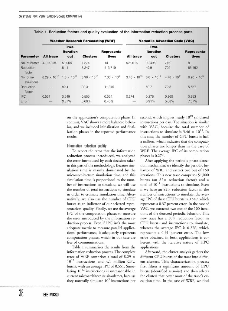
Table 1 summarizes the results from theinformation reduction process. The completetrace of WRF comprises a total of 8.29 �1012 instructions and 4.1 million CPUbursts, with an average IPC of 0.551. Simu-lating 1012 instructions is unreasonable incurrent microarchitecture simulators, becausethey normally simulate 105 instructions per

second, which implies nearly 1010 simulatedinstructions per day. The situation is similarwith VAC, because the total number ofinstructions to simulate is 3.46 � 1013. Inthis case, the number of CPU bursts is halfa million, which indicates that the computa-tion phases are longer than in the case ofWRF. The average IPC of its computationphases is 0.274.

After applying the periodic phase detec-tion mechanism, we identify the periodic be-havior of WRF and extract two out of 160iterations. This new trace comprises 51,000bursts (an 82� reduction factor) and atotal of 1011 instructions to simulate. Evenif we have an 82� reduction factor in thenumber of instructions to simulate, the aver-age IPC of these CPU bursts is 0.549, whichrepresents a 0.37 percent error. In the case ofVAC, we extracted two out of the 100 itera-tions of the detected periodic behavior. Thisnew trace has a 50� reduction factor inCPU bursts and instructions to simulate,whereas the average IPC is 0.276, whichrepresents a 0.91 percent error. The lowerror obtained in both applications is co-herent with the iterative nature of HPCapplications.

Afterward, the cluster analysis gathers thedifferent CPU bursts of the trace into differ-ent clusters. This characterization processfirst filters a significant amount of CPUbursts (identified as noise) and then selectsthe clusters that cover most of the trace’s ex-ecution time. In the case of WRF, we find

[3B2-9] mmi2011030032.3d 23/5/011 14:59 Page 38

Table 1. Reduction factors and quality evaluation of the information reduction process parts.

Weather Research Forecasting (WRF) Versatile Advection Code (VAC)

Parameter All trace

Two-

iteration

cut Clusters

Representa-

tives All trace

Two-

iteration

cut Clusters

Representa-

tives

No. of bursts 4,137,194 51,008 1,274 10 523,616 10,495 746 8

Reduction

factor

— 81.1 3,247 413,719 — 49.9 702 65,452

No. of in-

structions

8.29 � 1012 1.0 � 1011 8.98 � 1010 7.30 � 108 3.46 � 1013 6.8 � 1011 4.78 � 1011 6.20 � 109

Reduction

factor

— 82.4 92.3 11,345 — 50.7 72.5 5,587

IPC 0.551 0.549 0.555 0.554 0.274 0.276 0.260 0.253

Error — 0.37% 0.60% 0.40% — 0.91% 5.08% 7.57%

....................................................................

38 IEEE MICRO

...............................................................................................................................................................................................

SYSTEMS FOR VERY LARGE-SCALE COMPUTING

five clusters, covering 88 percent of the totalexecution cycles. These clusters represent1,274 CPU bursts (a 3,200� reduction fac-tor) with a total of 8.98 � 1010 instructionsto simulate (a 92� reduction factor). The re-duction in CPU bursts is around one orderof magnitude larger than the reduction ininstructions to simulate. This fact indicatesthat the clustering analysis effectively filtersthe CPU bursts that aren’t representativein terms of execution time and IPC. Despitethe large reduction in instructions to simu-late, the average IPC of these five clusters is0.555, which represents a 0.60 percenterror. We obtained similar conclusions inthe case of VAC, where only two clusterscover 81 percent of execution time, with a700� and 70� reduction in CPU burstsand instructions to simulate, respectively,with an average IPC of 0.260, which repre-sents a 5.08 percent error.

Finally, we must select a set of representa-tives from the identified clusters of CPUbursts. In the case of WRF, we select tworepresentatives per cluster at random. Conse-quently, the number of selected CPU burstsis 10, and the number of instructions to sim-ulate is 7.3 � 108 (a 11,300� reduction fac-tor). The average IPC of these CPU bursts is0.554, which represents only a 0.40 percenterror with respect to the original trace. Be-cause the number of identified clusters inVAC is lower, we select four representativesper cluster. Here, the total number of CPUbursts is eight, whereas the number ofinstructions to simulate is 6.2 � 109

(a 5,587� reduction factor). The averageIPC of these CPU bursts is 0.253, whichrepresents a 7.57 percent error with respectto the original trace.

Thus, combining these three techniquesin the information reduction process leadsto a reduction in simulation time betweenfour and five orders of magnitude, with asmall error in the global application’s IPC.This huge reduction in simulation timewith high accuracy is due to the natural be-havior of HPC applications and the intelli-gence of the successive techniques used inthis information reduction process. As a re-sult, a parallel application that would requireseveral years of simulation time can be simu-lated in a few hours, obtaining at the same

time a detailed analysis at the microarchitec-ture and application levels.

Multilevel simulation qualityNext, we evaluate the error introduced by

the two simulators involved to simulate awhole supercomputer application. We firstfocus on self validation of the methodology,or predicting the execution time of the appli-cation in the same system in which it hadbeen executed. We then focus on cross valida-tion of the methodology, or predicting theexecution time of the parallel applicationson a different system configuration.

Self validation. As we described earlier, weuse MPsim, an in-house microarchitecturesimulator with a detailed pipeline andcache hierarchy. MPsim has been developedto perform research in the processor’smicroarchitecture. Thus, this simulator’starget architectures are future architecturesthat will appear in the market in about10 years. For this reason, the accuracywhen modeling a particular existing micro-architecture isn’t as important as the relativedifferences when projecting the perfor-mance of future architectures.

To predict the performance of the chosenHPC parallel applications running in a realmachine, we carefully chose the simulatorparameters to model a PowerPC 970-likeprocessor. Table 2 summarizes this machine’smain characteristics.

Table 3 shows the IPC values obtainedwith MPsim and those measured on ourreal supercomputer. In the case of WRF,the IPC predictions obtained with MPsimare always within 40 percent and, on average,25.16 percent different from the real IPC. Inthe case of VAC, the error per cluster re-mains within 40 percent, whereas the averageerror increases to 33.1 percent. We observethat the performance of CPU bursts over100 million instructions is normally overesti-mated, whereas the performance of shorterCPU bursts is underestimated. For shorttraces, recovering the state of the cache hier-archy implies a significant portion of simula-tion time. On the real machine, part of thisdata is already on the cache hierarchy,which reduces the execution time of thesecomputation phases. We’ve measured that

[3B2-9] mmi2011030032.3d 23/5/011 14:59 Page 39

....................................................................

MAY/JUNE 2011 39

it takes more than 5 million cycles. In con-trast, this initialization time is less significantfor longer traces. In this case, the overestima-tion is due to some structures optimisticallymodeled in MPsim: memory is assumedto be perfect (we assume that we will not ac-cess the disk). Also, some implementationdetails of the PowerPC 970 processor aren’tpublic, and we’ve followed a best-effortapproach.

Reducing the average IPC error ofMPsim is outside this article’s scope. Moreaccurate simulators exist, but they’re nor-mally industrial simulators developed bythe company selling the processor. These

simulators are more detailed (and slow),but show IPC estimations within a 1 percenterror. Because selecting the microarchitec-ture simulator is orthogonal to the presentedsimulation methodology, we report the errorin execution time when using the IPCobtained with MPsim or the real IPC thatwould be obtained with an industrialsimulator.

Finally, we simulate the original tracewith Dimemas10 using the microarchitecturesimulator’s feedback. Table 4 shows the ref-erence parameters used in the differentexperiments. This configuration models theMareNostrum supercomputer, composed of

[3B2-9] mmi2011030032.3d 23/5/011 14:59 Page 40

Table 2. Baseline MPsim processor configuration.

Features Specifications

Architecture 2 cores, 2-way symmetric multithreading (SMT),

superscalar architecture

Fetch, issue, and retire width 8, 5, and 5 instructions per cycle, respectively

Fixed-point and load/store issue queue 36 entries

Floating-point issue queue 20 entries

Branch-instructions issue queue 12 entries

CR-logical-instructions issue queue 10 entries

Vector-instructions issue queue 36 entries

Reorder buffer 100 entries

Branch predictor 16K-entry gshare*

Level 1 (L1) instruction cache 64 Kbyte, direct mapped, 128-byte line, 1 cycle hit

L1 data cache 32 Kbyte, 2-way, 128-byte line, 2 cycle hit, last recently

used (LRU)

L2 unified cache 1 Mbyte, 8-way, 128-byte line, 15 cycle latency, LRU

Memory latency 250 cycles

Peak memory bandwidth 2 GBps per GHz.................................................................................................................................*Two-level adaptive predictor with globally shared history buffer and pattern history.Commonly used in most current processors.

Table 3. Real IPC vs. MPsim predicted IPC comparison in self-validation

experiment, using two threads per core configuration.

WRF VAC

Cluster

number

Real

IPC

MPsim

IPC Error (%)

Real

IPC

MPsim

IPC Error (%)

1 0.529 0.703 32.77 0.289 0.380 31.71

2 0.497 0.466 �6.39 0.251 0.340 35.38

3 0.618 0.429 �30.72 — — —

4 0.755 0.468 �38.04 — — —

5 0.811 0.522 �35.60 — — —

Weighted average error (%) 25.16 Weighted average error (%) 33.12

....................................................................

40 IEEE MICRO

...............................................................................................................................................................................................

SYSTEMS FOR VERY LARGE-SCALE COMPUTING

clusters of IBM JS21 server blades. Eachnode has two PowerPC 970MP processors(four cores total) and 8 Gbyte of RAMmemory. The nodes are connected using aMyrinet network. In this table, memoryand network latency refer to the timeadded by the simulator to each communica-tion, in terms of library initialization, not theactual latency of these units.

Figure 2a shows the error in the total ex-ecution time of two iterations of the parallelapplication predicted with Dimemas, as wellas of the whole application error after apply-ing the cut factor. Using the IPC providedby MPsim, we obtain 7.67 percent error inthe execution time prediction of two itera-tions of WRF. This error is reduced to6.25 percent when predicting the executiontime of the whole application. Using theIPC values measured on the real machine(or a highly accurate industrial simulator),the error is reduced to just 0.3 percent fortwo iterations and 1.62 percent for thewhole application. This error is computableto the error introduced by Dimemas. Inthe case of VAC, the error increases to 16.2percent (two iterations) and 21.7 percent(full application) with MPsim values, and0.54 percent (two iterations) and 7.2 percent(full application) with the real IPC values.Thanks to the combination of communica-tion and computation phases, the initialerror of MPsim in IPC predictions is nearlydivided by 3 in the final prediction of execu-tion time.

Cross validation. We can use our simulationmethodology to predict the performance ofa parallel application when running on adifferent system configuration. More specif-ically, we can predict the parallel applica-tion’s execution time when running onetask per node (single-thread configuration)instead of four tasks per node (CMP config-uration). Nodes in our supercomputerinfrastructure comprise two dual-core pro-cessors with a shared Level 2 (L2) cache. Fur-thermore, the two chips share the 8 Gbytesof memory. We’ve run the applicationusing four tasks per node configuration andpredicted the performance when usingone task per node configuration. To cross

[3B2-9] mmi2011030032.3d 23/5/011 14:59 Page 41

(a)

25%

WRF.128 VAC.128

20%

15%10%5%0%

(b)

100%

WRF.128 VAC.128

80%

60%40%20%0%

Two iterations Two iterations + MPsim ratiosFull application Full application + MPsim ratios

Two iterations Two iterations + MPsim ratiosFull application Full application + MPsim ratios

Figure 2. Execution time prediction error for Versatile Advection Code (VAC) and Weather Research Forecasting (WRF)

parallel applications, for both self validation (a) and cross validation (b) experiments. The figures show the error when

estimating the execution time of two iterations of the application or the full application execution time with the measured

real IPC and the IPC provided by MPsim.

Table 4. Baseline Dimemas

cluster configuration.

Feature Specifications

No. of nodes 2,560

Processors per node 4

Input links per node 1

Output links per node 1

No. of buses 1*

Memory bandwidth

per node

600 Mbyte/s

Memory latency 4 ms

Network bandwidth 250 Mbyte/s

Network latency 8 ms.......................................................*Contention is only defined by inputand output links.

....................................................................

MAY/JUNE 2011 41

validate the results, we reran the applicationusing one task per node and compared itsruntime with the prediction.

First, we used MPsim to simulate adual-core PowerPC 970-like machine, asdescribed in Table 2, with just one represen-tative of each cluster running. Then we rantwo representatives of the same cluster inthe same processor configuration. The per-formance improvement per representativeis used as the required CPU ratio to the feed-back Dimemas simulator. Finally, Dimemassimulations are done with the cluster param-eters of the new configuration (we have justone processor per node instead of four asin Table 4).

Figure 2b shows the average error resultswe obtained. Without using the CPU ratiosderived from MPsim, we obtain 8.6 percentand 76.7 percent errors in the execution timeof two iterations of WRF and VAC, respec-tively. When predicting the whole applica-tion’s execution time, the error is reducedto 2.78 percent and 51.9 percent for WRFand VAC, respectively. The difference inthe error is due to the fact that VAC perfor-mance is much more affected than WRF

when moving from a configuration withone task per node to four tasks per node.When using the CPU ratios from MPsim,we reduce the error to 4.94 percent and56.5 percent for two iterations of WRFand VAC, respectively. In the case ofWRF, the measured CPU ratios for thefive representative clusters are between 1.05and 1.21, as Table 5 shows. The predictedratios are between 1.02 and 1.25, with an av-erage error of 5.3 percent in the CPU ratios.As a result, the final error in the whole appli-cation’s execution time prediction is just6.04 percent.

In the case of VAC, the measured CPUratios for the two representative clusters are1.75 and 1.92 (see Table 6). The predictedratios are 1.04 and 1.05, with an averageerror of 58.3 percent in the CPU ratios.This high error is due to the optimisticmodel of RAM memory implemented inMPsim. As we mentioned earlier, memoryis assumed to be perfect, with no misses.VAC is suffering between nine and 11 L2misses per kilo instruction, whereas WRFsuffers only between one and two L2 missesper kilo instruction. Apart from that, VAC

[3B2-9] mmi2011030032.3d 23/5/011 14:59 Page 42

Table 5. WRF cross-validation of MPsim ratios, comparing the IPC running two threads per core

(CMP) and a single thread per core, and the differences with the ratios in real configuration.

Task 7 Task 9

WRF

IPC

CMP

IPC single

thread Ratio

IPC

CMP

IPC single

thread Ratio

Representative

average ratio

Real

ratio

Error

(%)

Cluster 1 0.705 0.717 1.017 0.700 0.712 1.017 1.017 1.047 �2.90

Cluster 2 0.494 0.505 1.022 0.437 0.445 1.018 1.020 1.083 �5.82

Cluster 3 0.428 0.479 1.119 0.429 0.481 1.121 1.120 1.275 �12.18

Cluster 4 0.466 0.512 1.099 0.469 0.517 1.102 1.101 1.251 �12.04

Cluster 5 0.518 0.647 1.249 0.526 0.655 1.245 1.247 1.169 6.68

Weighted average error (%) �4.62

Table 6. VAC cross-validation of MPsim ratios and the differences with real ratios.

We express just the ratios, not the IPC, on single-thread and CMP configurations

because of the higher number of representatives.

VAC

Task 51

ratio

Task 79

ratio

Task 85

ratio

Task 104

ratio

Representative

average ratio

Real

ratio

Error

(%)

Cluster 1 1.048 1.049 1.053 1.049 1.050 1.756 �40.22

Cluster 2 1.042 1.042 1.042 1.039 1.041 1.937 �46.28

Weighted average error (%) �42.54

....................................................................

42 IEEE MICRO

...............................................................................................................................................................................................

SYSTEMS FOR VERY LARGE-SCALE COMPUTING

suffers much more TLB misses than WRF(a 2.5� increase). As a result, the final errorin execution time prediction of the whole ap-plication is 34.5 percent. Even if this accuracyis acceptable for our experiments, a moredetailed model of the memory hierarchy isrequired in the microarchitecture simulatorto obtain a more accurate prediction.

Performance analysisThis last experiment aimed to illustrate

our simulation methodology’s potential. Inparticular, we studied in detail the evolutionof the behavior of the applications as thesize of the L2 cache and network bandwidthincreased. This kind of performance analysisis not feasible if we must simulate the wholeapplication at the microarchitecture level,because simulating just one configurationwith a given L2 size would require severalyears of simulation time. Instead, weobtained our results with less than 1 dayof simulation.

Figure 3a shows results extracted from theVAC application in terms of IPC. In thiscase, we’ve divided the computing timeinto two clusters. From the perspective ofthe L2 cache size, we can see the same behav-ior in these two clusters—that is, a remark-able increase of the application’s IPC if theL2 cache is larger than 2 Mbytes. Themost important conclusion we can extractfrom this is that we can improve this applica-tion’s performance by executing it on asupercomputing infrastructure whose pro-cessors have an L3 cache level that can reducethe cycles dedicated to access principal mem-ory due to L2 misses. In Figure 3c, we depictthe same results for the WRF application.In this case, we can see a strong improvementof the performance in all the clusters until1 Mbyte of the L2 cache size is reached.This behavior is due to the small size ofthe input data. Thus, WRF will have enoughwith a small L2 cache to reach its maximumperformance.

[3B2-9] mmi2011030032.3d 23/5/011 14:59 Page 43

0.8

Cache size(a) (b)

(d)(c)

0.6

0.4

0.2

0

512 M

B

256 M

B

128 M

B

64 M

B

32 M

B

16 M

B

8 MB

4 MB

2 MB

1 MB

512 K

B

256 K

B

128 K

B

64 K

B

512 M

B

256 M

B

128 M

B

64 M

B

32 M

B

16 M

B

8 MB

4 MB

2 MB

1 MB

512 K

B

256 K

B

128 K

B

64 K

B

512 M

B

256 M

B

128 M

B

64 M

B

32 M

B

16 M

B

8 MB

4 MB

2 MB

1 MB

512 K

B

256 K

B

128 K

B

64 K

B

512 M

B

256 M

B

128 M

B

64 M

B

32 M

B

16 M

B

8 MB

4 MB

2 MB

1 MB

512 K

B

256 K

B

128 K

B

64 K

B

IPC

0.8

Cache size

0.6

0.4

0.2

0

IPC

70

Cache size

60

50

40

30

Tim

e (s

)

500

Cache size

450

400

350

300

Tim

e (s

)

Cluster 1 Cluster 2 250 Mb/s 500 Mb/s 125 Mb/s

250 Mb/s 500 Mb/s 125 Mb/s

Cluster 1 Cluster 2 Cluster 3Cluster 4 Cluster 5

Figure 3. Performance predictions of VAC and WRF using different cache sizes and network bandwidths. We present IPC

(a) and execution time (b) of VAC and the IPC (c) and execution time (d) of WRF.

....................................................................

MAY/JUNE 2011 43

Figures 3b and 3d show the executiontimes obtained with Dimemas after thecluster IPC ratios. This approach lets usstudy the impact of architectural parameters(in this case, L2 cache size) and networkparameters (in this case, bandwidth) simul-taneously. According to our results, the im-pact of the network is negligible in the caseof VAC and WRF. For these applications,the dominant performance factor is IPC,which significantly changes with the L2cache size.

O ur method is based on the perfor-mance isolation provided by the MPI

programming model and the distributedmemory cluster architecture. The computa-tional performance of one MPI task doesn’tdepend on what happens with the otherparallel tasks. The same isolation propertycan be observed on task-based program-ming models and DMA-based architectures.

Shared-memory programming modelssuch as OpenMP or a mixed MPI+OpenMPapplication would require simulating incycle-accurate mode all the CPU bursts exe-cuting on the shared-memory node to ac-count for the impact of the cache coherencyprotocol, limiting our method to clusterarchitectures with nodes featuring only afew shared-memory processors.

Our most immediate future work includesextending this methodology to other pro-gramming models that maintain the task in-dependence assumption. Further research isalso ongoing to extend this methodology tolarge-scale shared-memory systems. M I CR O

AcknowledgmentsThis work has been supported by the

Ministry of Science and Technology ofSpain under contract TIN2007-60625, bythe HiPEAC European Network of Excel-lence, and by the IBM/BSC MareIncognitoProject.

....................................................................References

1. E.A. Brewer et al., ‘‘PROTEUS: A High-

Performance Parallel-Architecture Simulator,’’

Proc. ACM SIGMETRICS Joint Int’l Conf.

Measurement and Modeling of Computer

Systems, ACM Press, 1992, pp. 247-248.

2. J.E. Miller et al., ‘‘Graphite: A Distributed

Parallel Simulator for Multicores,’’ Proc.

16th IEEE Int’l Symp. High Performance

Computer Architecture, IEEE Press, 2010,

doi:10.1109/HPCA.2010.5416635.

3. E. Argollo et al., ‘‘COTSon: Infrastructure for

Full System Simulation,’’ ACM SIGOPS

Operating Systems Review, vol. 43, no. 1,

2009, pp. 52-61.

4. E.S. Chung et al., ‘‘A Complexity-Effective

Architecture for Accelerating Full-System

Multiprocessor Simulations Using FPGAs,’’

Proc. 16th Int’l ACM/SIGDA Symp. Field

Programmable Gate Arrays, ACM Press,

2008, pp. 77-86.

5. E. Perelman et al., ‘‘Using SimPoint for Ac-

curate and Efficient Simulation,’’ Proc. ACM

SIGMETRICS Int’l Conf. Measurement and

Modeling of Computer Systems, ACM

Press, 2003, pp. 318-319.

6. R.E. Wunderlich et al., ‘‘SMARTS: Accelerat-

ing Microarchitecture Simulation via Rigorous

Statistical Sampling,’’ ACM SIGARCH Com-

puter Architecture News, vol. 31, no. 2,

2003, pp. 84-97.

7. M. Casas, R.M. Badia, and J. Labarta, ‘‘Au-

tomatic Structure Extraction from MPI

Applications Tracefiles,’’ Proc. Int’l Euro-

Par Conf. Parallel Computing, LNCS 4641,

Springer, 2007, pp. 3-12.

8. M. Ester et al., ‘‘A Density-Based Algorithm

for Discovering Clusters in Large Spatial

Databases with Noise,’’ Proc. 2nd Int’l

Conf. Knowledge Discovery and Data Min-

ing, AAAI Press, 1996, pp. 226-231.

9. J. Gonzalez, J. Gimenez, and J. Labarta,

‘‘Automatic Detection of Parallel Applications

Computation Phases,’’ Proc. IEEE Int’l Symp.

Parallel & Distributed Processing, IEEE CS

Press, 2009, doi:10.1109/IPDPS.2009.5161027.

10. S. Girona, J. Labarta, and R.M. Badia, ‘‘Val-

idation of Dimemas Communication Model

for MPI Collective Operations,’’ Proc. 7th

European PVM/MPI Users’ Group Meeting

on Recent Advances in Parallel Virtual

Machine and Message Passing Interface,

Springer, 2000, pp. 39-46.

11. G. Toht, ‘‘Versatile Advection Code,’’ Proc.

Int’l Conf. Exhibition on High-Performance

Computing and Networking, Springer, 1997,

pp. 253-262.

12. J. Michalakes et al., ‘‘The Weather

Research and Forecast Model: Software

[3B2-9] mmi2011030032.3d 23/5/011 14:59 Page 44

....................................................................

44 IEEE MICRO

...............................................................................................................................................................................................

SYSTEMS FOR VERY LARGE-SCALE COMPUTING

Architecture and Performance,’’ Proc. 11th

ECMWF Workshop Use of High Perfor-

mance Computing in Meteorology, World

Scientific Books, 2004, pp. 156-168.

Juan Gonzalez is a researcher at theBarcelona Supercomputing Center and aPhD student in the Computer ArchitectureDepartment of the Polytechnic University ofCatalonia. His research interests include theapplication of data-mining techniques to theautomatic performance analysis of parallelapplications. Gonzalez has an MS in com-puter science from the Polytechnic Univer-sity of Catalonia.

Marc Casas is a post-doctoral researchscholar at the Lawrence Livermore Na-tional Laboratory. His research interestsspan parallel computing, focusing on fault-tolerance and reliability of HPC applica-tions, scalability, and automatic performanceanalysis. Casas has a PhD in computerarchitecture from the Polytechnic Universityof Catalonia.

Judit Gimenez is a research manager at thePolytechnic University of Catalonia andthe Performance Tools Group managerat the Barcelona Supercomputing Center.Her research interests include parallelcomputing, focusing on developing per-formance analysis tools. Gimenez has anMS in computer science from the Poly-technic University of Catalonia.

Miquel Moreto is a lecturer in the Compu-ter Architecture Department at the Poly-technic University of Catalonia. His researchinterests include modeling parallel computersand resource sharing in multithreaded archi-tectures. Moreto has a PhD in computer

architecture from the Polytechnic Universityof Catalonia.

Alex Ramirez is an associate professor at thePolytechnic University of Catalonia and aresearch manager at the Barcelona Super-computing Center. His research interestsinclude heterogeneous multicore architec-tures, hardware support for programmingmodels, and simulation techniques. Ramir-ez has a PhD in computer science from thePolytechnic University of Catalonia.

Jesus Labarta is a professor at the Poly-technic University of Catalonia and directorof the Computer Science Department ofthe Barcelona Supercomputer Center. Hisresearch interests include high-performancearchitectures and system software, particu-larly programming models and performancetools. Labarta has a PhD in telecommunica-tions from the Polytechnic University ofCatalonia.

Mateo Valero is a professor at the Poly-technic University of Catalonia and directorof the Barcelona Supercomputer Center. Hisresearch interests include high-performancearchitectures. Valero has a PhD in telecom-munications from the Polytechnic Universityof Catalonia. He’s a fellow of IEEE and theACM and a Distinguished Research Fellowat Intel.

Direct questions and comments aboutthis article to Juan Gonzalez, Campus NordUPC � C6 Building Office 002, c/JordiGirona, 1-3, 08034 Barcelona, Spain;juan.gonzalez@bsc.es.

[3B2-9] mmi2011030032.3d 23/5/011 14:59 Page 45

....................................................................

MAY/JUNE 2011 45