Embed Size (px)
Citation preview

Mat-2.177 Project Seminar in Operational Research
Report, Group Nokia 1
Mobile Phones Replacement Forecasting:
Theories and Drivers
April 24, 2003
_____________________________________________________________________
Lari Hämäläinen 51623A
Veera Lattunen 54349L
Riikka-Leena Leskelä 55406C
Hanna Niemi 55438T
Timo Similä 49935D

Replacement modeling benchmarks and indicators of change -Hämäläinen, Lattunen, Leskelä, Niemi, Similä-
2
Executive Summary
Replacement market is getting more and more important as the new customer market
saturates. So far the market forecasting methods have emphasized the new customer
business and the replacement market forecasting has been insufficiently sophisticated.
This paper approaches replacement demand forecasting from two directions: Firstly, it
explains some models of replacement demand found from the literature. Secondly, it
explores drivers for replacement behavior.
Unfortunately the literature overview reveals no directly applicable models, but the
models examined are all helpful. Duration model would have required accurate data
on the age and life cycles of the mobile phones in use, from which the former poses a
problem: the age could only be estimated or acquired through a survey, because there
is no data on which devices are replaced and which ones still are in use. A generation-
based approach was not directly applicable to mobile phones. The bottom-up-
approach using aspiration levels of phone users seemed interesting but it was not
easily convertible to the case at hand. The idea to start from the motivation vs. cost of
replacing that was used in the search for drivers was, however, inspired by this
approach. Finally, the approach of using probability functions to describe life cycles
seemed feasible, but would require analysis on how the life cycles could be estimated.
The four groups of drivers identified for replacement of a functional phone were
technological change, subsidy policy of the operators, change in the consumption
ability and the price of the mobile phones. The applicability of some consumption
ability indicators was analyzed against recent development of replacement demand.
The data, however, was somewhat insufficient for the purpose of verifying the drivers,
and although the analysis showed that there exist correlations between replacement
sales and different parameters, such as GDP, these relations were not consistent across
different markets. Due to the fast increase in the amount of cellular phones also the
amount of replacement sales has increased independent of many economic drivers.
The next step would be to include drivers of other categories and examine their
applicability in estimating the life cycles in mature markets.

Replacement modeling benchmarks and indicators of change -Hämäläinen, Lattunen, Leskelä, Niemi, Similä-
3
Table of Contents
1 INTRODUCTION.........................................................................................................................5
1.1 BACKGROUND........................................................................................................................5
1.2 RESEARCH PROBLEM AND OBJECTIVES..................................................................................6
1.3 FOCUS OF THE STUDY ............................................................................................................6
1.4 STRUCTURE OF THE REPORT...................................................................................................7
2 THEORETICAL STUDY ............................................................................................................8
2.1 LITERATURE OVERVIEW ON REPLACEMENT DEMAND MODELING.........................................8
2.1.1 Observable and unobservable determinants of replacement of home appliances
(Fernandez 2001)............................................................................................................................8
2.1.2 A Choice-Based Diffusion Model for Multiple Generations of Products (Jun and Park
1999) 10
2.1.3 Modelling diffusion and replacement (Islam and Meade 2000) .....................................14
2.1.4 Environmentally friendly replacement of automobiles (Marell, Davidson and Gärling
1995) 17
2.2 DISCUSSION ON FINDINGS OF LITERATURE OVERVIEW ........................................................21
3 PRACTICAL STUDY ................................................................................................................23
3.1 PRACTICAL REQUIREMENTS OF REPLACEMENT FORECASTING MODELS..............................23
3.2 DRIVERS FOR REPLACEMENT DEMAND ................................................................................24
3.2.1 Indicators of Change in Consumption Ability ................................................................25
3.2.2 Price of Mobile Phones ..................................................................................................26
3.2.3 Subsidy Policy of the Operators .....................................................................................26
3.2.4 Technological Change....................................................................................................27
3.3 EVALUATION OF THE DRIVERS.............................................................................................28

Replacement modeling benchmarks and indicators of change -Hämäläinen, Lattunen, Leskelä, Niemi, Similä-
4
3.4 DESCRIPTION OF THE DATA ..................................................................................................30
3.5 RESULTS..............................................................................................................................33
3.5.1 Correlations....................................................................................................................33
3.5.2 Linear Regression...........................................................................................................36
3.5.3 Discussion of the Results of the Correlation and Regression Analyses..........................40
CORRELATIONS................................................................................................................................40
3.6 NEURAL NETWORK- APPROACH...........................................................................................43
3.6.1 Visualizing variables with Self-Organizing Map............................................................43
4 CONCLUSIONS .........................................................................................................................50
5 REFERENCES............................................................................................................................52
APPENDICES ......................................................................................................................................54
5.1 APPENDIX 1 – CORRELATIONS.............................................................................................54
5.2 APPENDIX 2 - PROJECT.........................................................................................................57
5.2.1 Phases.............................................................................................................................57
5.2.2 Workload ........................................................................................................................59
5.2.3 Lessons learned ..............................................................................................................61

1 Introduction
1.1 Background
As the first-time buyer market for mobile phones is saturating, the interest of the
handset manufacturers is drawn to the old customers replacing their current device.
The replacement market differs from the new customer market, and so the
replacement demand needs to be forecasted separately from the demand of the new
customer market. The client (Nokia Mobile Phones) does have methods for
forecasting replacement demand, but the market forecasting methods have
emphasized the new customer business. Figure 1 illustrates the standpoint of this
study for evaluating replacement demand. Our primary focus is on “The share of
consumers replacing”.
Demand of replacing a broken device
Replacement demand
Overall demand
New users
Demand of replacing a functional device
The amount of phones in use
The amount of phones in use
The share of consumers replacing
The share of broken devices
Demand of replacing a broken device
Replacement demand
Overall demand
New users
Demand of replacing a functional device
The amount of phones in use
The amount of phones in use
The amount of phones in use
The amount of phones in use
The share of consumers replacing
The share of consumers
The share of broken devices The share of broken devices
Figure 1 The overall picture of replacement demand. The amount of replacements of
mobile phones is a function of the amount of phones in use and the share of the owners
replacing their device.

Replacement modeling benchmarks and indicators of change -Hämäläinen, Lattunen, Leskelä, Niemi, Similä-
6
1.2 Research Problem and Objectives
The research problem is the following: How should replacement demand of mobile
phones be forecasted?
The research problem is divided into the following questions:
� What are the models for replacement demand forecasting described in the
academic literature?
o Can these models be used in the Nokia case?
� Are there external drivers, based on which the replacement demand could be
forecasted?
The objectives of the study are the following:
� To find ideas for replacement modeling from the literature
� To find drivers for changes in replacement demand and test how well they
explain changes in replacement demand
1.3 Focus of the Study
The literature review will take a more general perspective on replacement modeling,
whereas the practical part will be more focused. In the following, the focus of the
practical study is described and justified.
Replacement demand consists of replacements of broken devices and devices that do
not meet with the aspiration level of the consumer anymore. The share of broken
devices is probably quite constant, whereas substitution of functional devices is more
variable. This is why our analysis on indicators focuses on the situation where the
current devise is still working. The data we have on replacement sales includes both
kinds of replacement, but the changes in the level of replacement demand are mostly
due to consumers replacing an operable phone.

Replacement modeling benchmarks and indicators of change -Hämäläinen, Lattunen, Leskelä, Niemi, Similä-
7
The study on indicators focuses on the factors indicating change in the share of
mobile phone users replacing their handsets. The actual number of replacement
demand requires information on the past sales so that the number of mobile phones
currently in use can be calculated. This is taken into account in the analysis on data.
Forming a complete model of replacement demand forecasting is not in the scope of
this paper. The search for drivers ultimately serves the purpose of forming such
models, so the requirements a good model poses on the drivers have to be taken into
account.
1.4 Structure of the Report
The report is organized in four parts: introduction, theoretical approach, practical
approach and conclusions. The theoretical approach includes a review of the literature
concerning replacement demand modeling and discusses the findings with regard to
the client. Practical approach deals with the drivers for replacement demand- first
explaining which factors could indicate changes in replacement demand of mobile
phones and then testing the reliability of the drivers. The last section of the part will
conclude the findings. Finally, the results are summarized and discussed in the last
part of the report.

Replacement modeling benchmarks and indicators of change -Hämäläinen, Lattunen, Leskelä, Niemi, Similä-
8
2 Theoretical Study
The purpose of this section is to explore academic literature on the field of
replacement demand modeling. The approach we use is to summarize theories
brought up by four relevant articles and discuss their applicability and usefulness in
the case of Nokia.
2.1 Literature Overview on Replacement Demand Model ing
2.1.1 Observable and unobservable determinants of r eplacement
of home appliances (Fernandez 2001)
Duration models have lately become popular in modeling replacement purchase
behavior (Fernandez 2001). This is because they are better in analyzing complex
dynamic processes, such as choice behavior, than conventional discrete choice
models. The duration models are constructed to estimate the duration, i.e. the length
of some event. In stead of a regular probability distribution the duration models are
usually based on a hazard function (see e.g. Kiefer 1988). A hazard function is a
conditional probability function that is denoted here (t). The hazard function
describes the probability at which events will be ending at time t given that it had
lasted until time t. A hazard function is constructed as follows. Let the cumulative
distribution function be
F(t) = P(T < t) (1)
which specifies the probability that the random variable T is less than some given
value t. The corresponding density function is then
f(t) = dF(t)/dt (2)
The survivor function is defined as
S(T) = 1 – F(T) = P(T t)

Replacement modeling benchmarks and indicators of change -Hämäläinen, Lattunen, Leskelä, Niemi, Similä-
9
which is the complement of the cumulative function F(t) giving the probability that
the random variable is greater than some given value t. The hazard function is then
defined as
(t) = f(t)/S(t) (3)
The most commonly used distributions are the exponential distribution and the
Weibull distribution due to the fact that their hazard functions are rather simple and
thus convenient to use. The hazard functions of the normal and lognormal
distributions are much more complex.
When modeling economic behavior it is useful to add other components than time in
to the model as well. Lancaster (1979) and Kiefer (1988) add explanatory variables to
the model. Using a proportional hazard specification the function becomes
(t, x, , 0) = (x, ) 0(t) (4)
where 0 is a “baseline” hazard function, x is a vector containing the explanatory
variables and is a vector containing the coefficients of the variables. This means that
the distribution is identical for all events if considered only with respect to time. The
addition of the explanatory variables shifts the distributions up and down and along
the time axis. This brings differences between events in varying conditions defined by
the explanatory variables. The parameters of the model are estimated with the
maximum likelihood method.
Both Lancaster (1979) and Kiefer (1988) apply the duration model to analyzing
unemployment and re-employment. However, newer studies (e.g. Raymond et al.
1993 and Fernandez 2001) apply the duration model approach to the replacement of
home appliances. Raymond et al. state that hazard models allow for much richer
relationships between the ages of the goods and the probabilities of their replacement
than typical dependent variable models. Fernandez uses the duration model to analyze
observable and unobservable determinants of replacement of heating equipment and

Replacement modeling benchmarks and indicators of change -Hämäläinen, Lattunen, Leskelä, Niemi, Similä-
10
central air conditioning systems. She recognizes the importance of demographic and
lifestyle variables, perceived obsolescence, styling and fashion and environmental
awareness among other variables, on the likelihood of replacement and tries to take
them into consideration in the duration model. Using the hazard function approach
presented by Lancaster (1979) and Kiefer (1988) she adds explanatory variables –
regressors – into the model. She uses variables describing the wealth and
conservatism of the customers, the operating costs of the appliances and the usage of
the appliances (deprecation).
The duration model is very versatile; it is useful in studying both macro and
microeconomic phenomena. The general formulation of the hazard function allows for
many different variations simply through changing the explanatory variables.
However, the application of the hazard function approach requires that there is data on
the distribution of the ages of current appliances and the lengths of the life cycles of
the appliances. So, as such the duration model is not applicable to the case of Nokia
Mobile Phones (we don’t have the required data so that we could apply this model).
2.1.2 A Choice-Based Diffusion Model for Multiple G enerations of
Products (Jun and Park 1999)
Jun and Park (1999) develop a model that incorporates both diffusion and choice
effects to capture simultaneously the diffusion and replacement processes for each
successive generation of durable technology. The model differs from previous
diffusion models in that effects of exogenous variables such as price are incorporated
into the diffusion process by modeling choice behavior of the consumer. The model
also set low requirements on sales data, since replacement and first-purchase sales
mustn’t necessarily be distinguishable.
Replacement modeling benchmarks and indicators of change -Hämäläinen, Lattunen, Leskelä, Niemi, Similä-
11
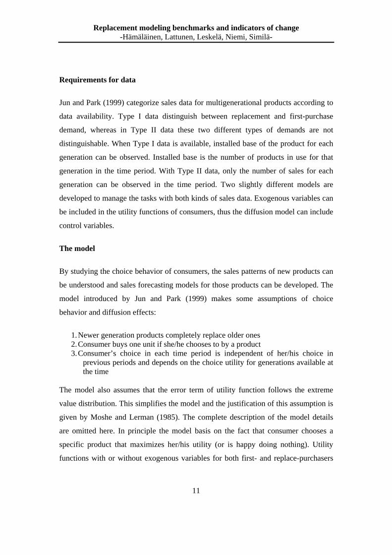
Requirements for data
Jun and Park (1999) categorize sales data for multigenerational products according to
data availability. Type I data distinguish between replacement and first-purchase
demand, whereas in Type II data these two different types of demands are not
distinguishable. When Type I data is available, installed base of the product for each
generation can be observed. Installed base is the number of products in use for that
generation in the time period. With Type II data, only the number of sales for each
generation can be observed in the time period. Two slightly different models are
developed to manage the tasks with both kinds of sales data. Exogenous variables can
be included in the utility functions of consumers, thus the diffusion model can include
control variables.
The model
By studying the choice behavior of consumers, the sales patterns of new products can
be understood and sales forecasting models for those products can be developed. The
model introduced by Jun and Park (1999) makes some assumptions of choice
behavior and diffusion effects:
1. Newer generation products completely replace older ones 2. Consumer buys one unit if she/he chooses to by a product 3. Consumer’s choice in each time period is independent of her/his choice in
previous periods and depends on the choice utility for generations available at the time
The model also assumes that the error term of utility function follows the extreme
value distribution. This simplifies the model and the justification of this assumption is
given by Moshe and Lerman (1985). The complete description of the model details
are omitted here. In principle the model basis on the fact that consumer chooses a
specific product that maximizes her/his utility (or is happy doing nothing). Utility
functions with or without exogenous variables for both first- and replace-purchasers

Replacement modeling benchmarks and indicators of change -Hämäläinen, Lattunen, Leskelä, Niemi, Similä-
12
are generated. With help of utility functions the following probabilities can be
estimated for Type I model
� The probability that the kth generation will be chosen from set of alternatives by first-purchaser at specific time.
� The probability that an ith generation user upgrades to the kth generation at specific time.
and for Type II model:
� The probability that a consumer (either first- or replacement demand) purchases kth generation product at specific time.
These probabilities are used in estimating the installed base for Type I data and the
number of sales of each product generation for Type II data.
Applications
Jun and Park (1999) introduce two applications of the model. The data used to
validate the Type I model consists of 24 yearly observations of sales data for four
successive generations of IBM computers from 1955 to 1978. The generations of
computers were launched: 1) vacuum tubes 1955, 2) transistors 1959, 3) integrated
circuits 1965, and 4) silicon chips 1971. The installed bases of each generation can be
observed and no exogenous variables, such as price, are available. The model is
applied to estimate the number of IBM computers representing the four possible
generations in use as a function of time.
The Type II model is tested with data consisting 46 quarterly observations of
worldwide shipments for four generations of DRAM memory from the 1st quarter of
1974 to the 2nd quarter of 1985. The generations of DRAM were launched: 1) 4k 1st
quarter of 1974, 2) 16k 3rd quarter of 1976, 3) 64k 1st quarter of 1979, and 4) 256k 4th
quarter of 1982. Only the number of quarterly shipments (not the number of products
in use) is available for each generation. The price per bit is available for this
Replacement modeling benchmarks and indicators of change -Hämäläinen, Lattunen, Leskelä, Niemi, Similä-
13
application as an exogenous variable. The model is applied to estimate the shipments
of different DRAM generations as a function of time.
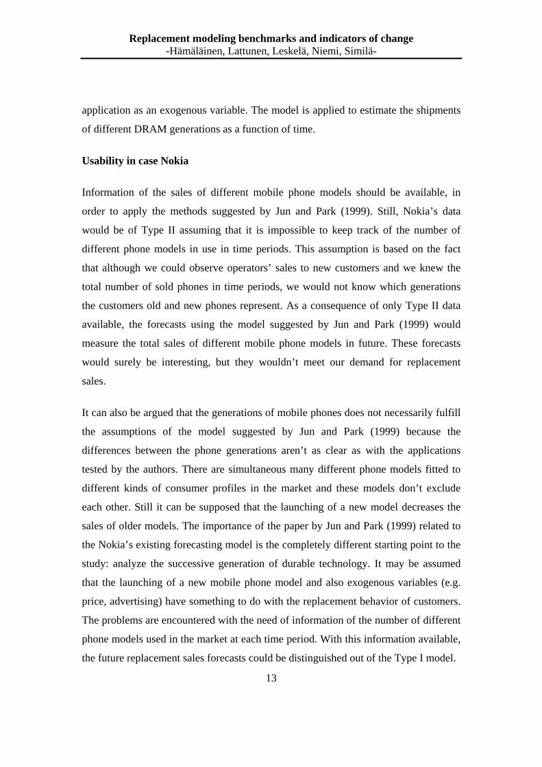
Usability in case Nokia
Information of the sales of different mobile phone models should be available, in
order to apply the methods suggested by Jun and Park (1999). Still, Nokia’s data
would be of Type II assuming that it is impossible to keep track of the number of
different phone models in use in time periods. This assumption is based on the fact
that although we could observe operators’ sales to new customers and we knew the
total number of sold phones in time periods, we would not know which generations
the customers old and new phones represent. As a consequence of only Type II data
available, the forecasts using the model suggested by Jun and Park (1999) would
measure the total sales of different mobile phone models in future. These forecasts
would surely be interesting, but they wouldn’t meet our demand for replacement
sales.
It can also be argued that the generations of mobile phones does not necessarily fulfill
the assumptions of the model suggested by Jun and Park (1999) because the
differences between the phone generations aren’t as clear as with the applications
tested by the authors. There are simultaneous many different phone models fitted to
different kinds of consumer profiles in the market and these models don’t exclude
each other. Still it can be supposed that the launching of a new model decreases the
sales of older models. The importance of the paper by Jun and Park (1999) related to
the Nokia’s existing forecasting model is the completely different starting point to the
study: analyze the successive generation of durable technology. It may be assumed
that the launching of a new mobile phone model and also exogenous variables (e.g.
price, advertising) have something to do with the replacement behavior of customers.
The problems are encountered with the need of information of the number of different
phone models used in the market at each time period. With this information available,
the future replacement sales forecasts could be distinguished out of the Type I model.

Replacement modeling benchmarks and indicators of change -Hämäläinen, Lattunen, Leskelä, Niemi, Similä-
14
2.1.3 Modelling diffusion and replacement (Islam an d Meade 2000)
Islam and Meade (2000) survey and evaluate different forecasting models for total
sales of consumer durables, which include both a diffusion component and a
replacement component. When estimating replacement demand, Islam and Meade
(2000) conclude that it is critical to estimate the lifetime of the consumer durable
accurately.
Replacement sales depend on the number and ages of consumer durables already sold.
The first modeling approach tries to decompose historical time series of total sales
into first time and replacement sales. Replacement sales are further divided into one
year old durables, two year old, and so on, which makes it possible to estimate crucial
replacement parameters for different probability functions. The second approach
taken is to use a model-free replacement process, where the shape of the distribution
of product lifetime is estimated from time series data.
The time series data sets available for calculations contained data from approximately
10-30 years.
Modeling Approach
Islam and Meade (200) model replacement sales using a density function � �Tf , which
is a function of the lifetime T of the product. Using this function the proportion of
durables that have survived i time periods can be calculated using a function called
survival function:
� � � ���
�i
dTTfiM .
Using the survival function the value of replacement sales at time can be calculated to
be
Replacement modeling benchmarks and indicators of change -Hämäläinen, Lattunen, Leskelä, Niemi, Similä-
15
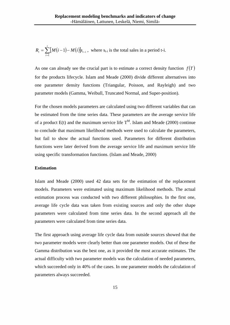
� � � �� ��
�t
titt siMiMR
1
1 , where st-i is the total sales in a period t-i.
As one can already see the crucial part is to estimate a correct density function � �Tf
for the products lifecycle. Islam and Meade (2000) divide different alternatives into
one parameter density functions (Triangular, Poisson, and Rayleigh) and two
parameter models (Gamma, Weibull, Truncated Normal, and Super-position).
For the chosen models parameters are calculated using two different variables that can
be estimated from the time series data. These parameters are the average service life
of a product E(t) and the maximum service life TM. Islam and Meade (2000) continue
to conclude that maximum likelihood methods were used to calculate the parameters,
but fail to show the actual functions used. Parameters for different distribution
functions were later derived from the average service life and maximum service life
using specific transformation functions. (Islam and Meade, 2000)
Estimation
Islam and Meade (2000) used 42 data sets for the estimation of the replacement
models. Parameters were estimated using maximum likelihood methods. The actual
estimation process was conducted with two different philosophies. In the first one,
average life cycle data was taken from existing sources and only the other shape
parameters were calculated from time series data. In the second approach all the
parameters were calculated from time series data.
The first approach using average life cycle data from outside sources showed that the
two parameter models were clearly better than one parameter models. Out of these the
Gamma distribution was the best one, as it provided the most accurate estimates. The
actual difficulty with two parameter models was the calculation of needed parameters,
which succeeded only in 40% of the cases. In one parameter models the calculation of
parameters always succeeded.

Replacement modeling benchmarks and indicators of change -Hämäläinen, Lattunen, Leskelä, Niemi, Similä-
16
The second approach using only time series information was even more complicated.
Here the demands on the data sets are far greater because more parameters have to be
estimated. It was found, that the parameter estimation rarely converged to allowable
values. For example in the case of Gamma distribution only 14% of the tests
succeeded.
Overall the success rate of valid parameter estimation was only in the range of 20-
40% for all models.
Summary
The different life cycle density functions were shown to provide a good
approximation for the life cycle of a durable good. The major difficulty was in the
parameter estimation and over half of the cases failed because of this.
In the end Islam and Meade (2000) concluded that just as good estimations can be
done using a distribution free approach, where does not use any specific distribution.
The needed “shape parameters” are roughly estimated from the data or be based on
expert opinion.
Case Nokia
For Nokia the article provides clear signals. First of all it should be understood that
the estimation of the parameters may not be possible from the existing data, especially
in a young and dynamic industry as telecommunications.
If the parameters are estimated using an expert opinion one should not necessarily use
any specific distribution function, but could do fine with a rough estimation of the
product life cycle from previous data.

Replacement modeling benchmarks and indicators of change -Hämäläinen, Lattunen, Leskelä, Niemi, Similä-
17
2.1.4 Environmentally friendly replacement of autom obiles (Marell,
Davidson and Gärling 1995)
Context of the study
Majority of purchases are replacements for products such as automobiles,
refrigerators, TVs, VCRs and CD players. According to previous studies product
failure is seldom an important reason for replacement. Instead market price,
advertising, styling and new features are found to have a greater impact. However the
timing of durable-replacement purchases has not been an important target for theories.
Not much literature on the topic exists.
Conceptual framework and study hypotheses
Marell, Davidson and Gärling (1995) hypothesize that an owned durable becomes a
candidate for replacement when assessed as being worse than consumer’s aspiration
level (i.e. the replacement purchase intention will increase). The aspiration level is
defined as a minimally acceptable quality (Simon 1955, 1956). The aspiration level
has a key role, because it is supposed to mediate influences of many factors, such as
expected changes in economy, changes in sociodemographic factors, changes in taste,
and marketing of technological innovations. The mediating affect of aspiration level
may be understood as an effect of directing attention towards different attributes. For
example, if styling is an important feature of a product then the quality of the
currently owned product will be more influenced by styling. Aspiration level both
changes and causes changes in the assessment of the current durable.
Marell et al. (1995) assume several mediating steps to take place before a replacement
is made. Conceptualization of these steps is presented in Figure 2.

Replacement modeling benchmarks and indicators of change -Hämäläinen, Lattunen, Leskelä, Niemi, Similä-
18
Economy
Technological innovations
Sociodemographic factors
Taste
Environmental concerns
Decline of
owned product
Current level
Competinggoals
Comparison
Goal setting
Aspirationlevel
Replacementpurchaseintention
Market search
Replacementpurchase
Figure 2 A conceptualization of factors affecting replacement purchase
Applied in the case of Nokia
The idea of the difference between aspiration level and perceived quality level as a
factor affecting in replacement purchases is very tempting. However, applying this
kind of approach into Nokia’s forecasting models would require totally new
procedures. The biggest question is how to define and measure aspiration levels and
perceived quality levels. If duplicating this article’s approach, Nokia should conduct
consumer surveys and measure aspiration level and perceived quality level by
questions. This method would be bottom-up instead of top-down, and would require
significant resources. For curiosity it is described next how the difference between
aspiration level and perceived quality level was studied in this particular case of
automobiles.

Replacement modeling benchmarks and indicators of change -Hämäläinen, Lattunen, Leskelä, Niemi, Similä-
19
Study objectives
� Whether the timing of replacement purchases is related to the difference
between owner’s assessment of the current quality of their automobile and
their aspiration level.
� Whether information indicating that either early or late replacement is better
for the environment affects the timing of replacement.
� Whether or not such an effect of information is mediated by changes in
aspiration level.
Method and sample
The researchers interviewed one hundred automobile owners in Sweden through a
telephone. Interviewees were randomly divided in two groups. For the first group it
was communicated that an early replacement of an automobile is better and for the
second group a late replacement was communicated to better in terms of environment.
The following information was gathered from each respondent.
� Sosiodemographic factors (household size, age of household members,
education, occupation, income)
� Factors related to the car and its usage (type and frequency of use, cost, year of
purchase, recent repair costs, number of other automobiles available to the
household.)
� Aspiration level (measured with a set of three questions, such as “Please
indicate on this scale (0=legal to drive to 100= brand new) what is the worst
level (lowest quality/lowest standard) of automobile you find acceptable to
own?” The aspiration level was then determined by average.)
� Environmental concern (measured with a set of seven questions on a scale
0=very little, 100=very much)
� Perceived level of quality (on the scale from 0 to 100 of their own car)
� Replacement purchase intention (timing)

Replacement modeling benchmarks and indicators of change -Hämäläinen, Lattunen, Leskelä, Niemi, Similä-
20
� Actual replacement purchases (from the national register of automobiles)
Results
Marell et al. (1995) used path analyses to examine whether replacement purchase
intention is related to the difference between aspiration level and current level.
Maximum-likelihood estimates were used to form two models. With the first model it
was found that all path coefficients reached significance except that associated with
the path from aspiration level to replacement purchase intention, which was only
marginally significant (see Figure 3). In the second model, which contained additional
factors, the age of the automobile was found to be insignificant and environmental
concern and income close to be significant. Other factors were found to affect as
predicted (see Figure 4).
Current level
Aspirationlevel
Replacementpurchaseintention
Replacementpurchase
-0.38***
0.19*
0.30***
0.32***
statisticalsignificance
*p<0.1
***p<0.01
Figure 3 Model 1

Replacement modeling benchmarks and indicators of change -Hämäläinen, Lattunen, Leskelä, Niemi, Similä-
21
Current level
Income
Replacementpurchaseintention
Aspirationlevel
Replacement
purchaseAutomobile age
Timingpreference
Environmentalconcern
Information
manipulation
0.3**
0.21*
0.36***
0.28**0.24**
0.19
-0.11 -0.38***
0.18*
statisticalsignificance
’p<0.1
*p<0.05
**p<0.01
***p<0.001
Figure 4 Model 2
As drawing a conclusion from Marell at al.’s study, it can be said that replacement
purchase intention was causally related to the current level and the aspiration level in
both models. Further the information (early replacement better/late replacement
better) given was found to affect the aspiration level.
2.2 Discussion on Findings of Literature Overview
Four different replacement forecasting approaches were just examined. There were
fundamental differences between each one of them as, for example, the approach
taken by Jun and Park (1999) meant that a totally new, generation based approach
would be needed. Marell, Davidson and Gärling (1995) in turn argued that by defining
aspiration levels one could adopt a bottom-up approach to replacement forecasting.
As good as these methods might be, they are out of our project’s scope.

Replacement modeling benchmarks and indicators of change -Hämäläinen, Lattunen, Leskelä, Niemi, Similä-
22
We also studied the dynamics of the duration model. The model was certainly
feasible, but the real problem was that one would need precise data on the ages of
current mobile phones and the lengths of the life cycles of these phones. If feasible
data is available the method provides a promising approach for Nokia to base their
estimations on. Islam and Meade (2000) suggested an easier way to forecast
replacement demand: we would just need to specify a probability function that would
describe life cycles of mobile phones. Just as with the duration model, the real
problem is to estimate the life cycle lengths correctly, as well as the maximum life
time of a phone.
With current data the estimates for the life cycle lengths and average life cycles are
hard to conduct, as not long enough time series are available. Mobile phones are a
relatively young market, where the constantly changing dynamics of the industry
make forecasting based on historical data almost impossible.
This brings us to our next question of what should be done to correct the situation.
The following chapter tries to give ideas to the problem and implicitly focus on the
question of what factors should be considered when estimating, for example, the
average life cycle of mobile phones.

Replacement modeling benchmarks and indicators of change -Hämäläinen, Lattunen, Leskelä, Niemi, Similä-
23
3 Practical Study
In this section, a more practically oriented point of view is taken compared to the
previous section with a theoretical emphasis. Now our goal is to give ideas that are
applicable with regard to the data and methods available. However, it should be
emphasized that the goal is not to give a direct answer to the problem of how to
forecast replacement demand, because forming a complete model would be beyond
the scope of this project. Instead, we aim at explaining what factors should be taken
into the model and proving this by using actual market data.
Before going into the details of the drivers, we shall explain what the requirements of
the model are, and hence, what is required from the drivers as well.
3.1 Practical Requirements of Replacement Forecasti ng
Models
Replacement forecasting methods should fulfill several requirements regarding
practicality. The model should be easy to explain, understand and challenge: both the
assumptions and the output of the model should be discussable also among people that
have no expertise on the field. This is highly important for two main reasons: the
model should be verifiable and open for further development if the assumptions of the
model are no longer valid.
The model should be parameterized in such a manner that most changes in the
replacement environment do not demand a change in the core of the model, but rather
in the parameters of the model.
The usability of the model is a significant characteristic. The model should be quick
and easy to use and the costs of the usage should not be excessive.

Replacement modeling benchmarks and indicators of change -Hämäläinen, Lattunen, Leskelä, Niemi, Similä-
24
Table 1Characteristics of a good replacement demand model
Understandability
Usability
Moderate costs of usage
Ideal drivers have the following characteristics: their values are known or at least
possible to forecast very accurately, the information should be inexpensive to gather,
and finally they should be both reliable and powerful predictors.
Table 2 Characteristics of good replacement drivers
Availability of forecasts/data
Inexpensiveness
Reliability of forecasts/data
Powerfulness as a predictor
3.2 Drivers for Replacement Demand
There are two fundamental factors affecting replacement demand for functional
mobile phones: the relative costs of replacement and the desirability of new phones. If
we are able to identify the most significant factors affecting replacement demand,
analyzing the change in these factors (variables) should reveal the change in
replacement demand. We shall thus call these factors drivers.
This chapter introduces and explores the usability of four groups of drivers for
replacement demand: 1) change in consumption ability, 2) price of mobile phones, 3)
subsidy policy of the telecom operators and 4) technological changes. The first three
capture the relative costs of replacement and the technological changes affect the
desirability of the new phones. The following Figure 5 demonstrates the identified
factors affecting replacement demand.

Replacement modeling benchmarks and indicators of change -Hämäläinen, Lattunen, Leskelä, Niemi, Similä-
25
3.2.1 Indicators of Change in Consumption Ability
The change in people’s ability to consume will have an effect on the sales of mobile
phones. One could conclude that the more money people have to spend the more they
will consume, which will directly affect the level of replacement sales.
To measure these changes we need to have indicators that fill the criteria introduced
in the beginning of chapter 3.1. Possible measures are for example gross domestic
products (GDP), consumer price indexes (CPI), wage indices, and different interest
rates. What makes the estimation difficult, are the fundamental differences between
different markets. Let us introduce a small example to clarify the dilemma. In market
1 the GDP has been growing steadily over the past 5 years and so has the replacement
sales. However, market 2 went into a recession when 3 years had passed and the GDP
actually fell, while the replacement rate grew.
The mobile phone market in general is in its infancy. General economic indicators
have existed for decades, while mobile phones have become common only in the
recent years. Due to this effect, the mobile phone penetration rate, as well as the
Desirability of replacement
Relative costs of replacement
Change in consumption abilities
Subsidy policy of the telecom operator
Price of mobile phones
Techological change
Replacement demand Desirability of
replacement
Relative costs of replacement
Change in consumption abilities
Subsidy policy of the telecom operator
Price of mobile phones
Techological change
Replacement demand Desirability of
replacement
Relative costs of replacement
Change in consumption ability
Subsidy policy of the telecom operator
Price of mobile phones
Techological change
Replacement demand
Figure 6 Factors affecting replacement demand

Replacement modeling benchmarks and indicators of change -Hämäläinen, Lattunen, Leskelä, Niemi, Similä-
26
amount of replacement sales, has increased almost independently of many indicators.
In the long run we can expect this relation to strengthen, which makes a factor to
consider.
3.2.2 Price of Mobile Phones
It is obvious that the price of mobile phones affects the willingness to buy a new one.
As prices drop and more attractive models are offered at lower prices, people are more
willing to replace their old ones.
One could say that it is enough just to measure the overall price across all mobile
phone categories. Our argument is, however, that the average price is likely to stay the
same over time, as new, more expensive models are constantly introduced. This forces
us to divide the market into different categories. We could for example classify
phones into three generic classes and calculate the average price for each one.
In reality the different prices are relatively hard to gather and the forecasting of price
development is almost impossible in a dynamic industry.
3.2.3 Subsidy Policy of the Operators
In most markets the operators subsidize mobile phones in order to tempt new
customers: the phone is bought as a package deal with the subscription, where the
price of the phone is not transparent. In such package deals the customer commits
himself or herself with the telecom operator for a given period of time. The level of
subsidy is an indicator of how small a share of the retail price of the phone is left to
the consumer to pay and how big a part is covered by the operator.
It is probable that the subsidies affect the replacement behavior: the customer is likely
to change the phone between the deals with the operator. Replacement is thus also
affected by the length of the contracts.

Replacement modeling benchmarks and indicators of change -Hämäläinen, Lattunen, Leskelä, Niemi, Similä-
27
One could think that the level of subsidies is similar to the price as an indicator. On
one hand it is, as subsidized phones seem cheaper to consumers, but on the other the
level of subsidies affects the extent to which the replacement behavior is dictated by
the telecom operators and their contract policy. If the level of subsidies is high and the
contracts short, replacement cycle is shorter than in situations where the level of
subsidies is low or the contracts are long. The following figure demonstrates the
relationships between level of subsidy, length of contract between the operator and the
customer, and the length of replacement cycle.
3.2.4 Technological Change
It is quite obvious that development of the products make replacement more tempting.
If there are only similar products in the market as the current device, there is only
little desire to replace it with the available models. The change in technology can be
gradual and incremental or totally disruptive. The transition from analogical mobile
phones to digital phones is an example of a technological discontinuity. Such
fundamental changes are still relatively rare. Minor technological changes include the
launch of SMS messages and color screens.
Length of contract
Length of replacement cycle
Level of subsidy
Length of contract
Length of replacement cycle
Level of subsidy
Figure 7 Subsidy policy affects length of replacement cycle

Replacement modeling benchmarks and indicators of change -Hämäläinen, Lattunen, Leskelä, Niemi, Similä-
28
Technological change is undoubtedly a very difficult indicator to measure. Firstly,
how could a discontinuity be distributed across time? The affects of discontinuities
often are distributed over a long time period. How should this be taken into account in
the model? Secondly, evaluating the significance of technological change is very
difficult beforehand. Comparing color screens against the ability to take pictures with
the phone sounds easier than it is. Who would have thought that SMS messages would
become such a success?
One way to overcome the problem could be to use expert opinion. Analysts could be
asked to assign a value between zero and one to describe the relevance of the
technological improvement: zero for a barely significant improvement and one for a
discontinuity. Also, the variable should be measured from the consumers’ point of
view. It should measure the perceived technological change rather than the actual
difference.
A less challenging indicator would be, for example, the number of phone models in
the market, which is fairly easily estimated.
3.3 Evaluation of the Drivers
In this chapter the drivers are evaluated against the criteria for a good indicator:
availability of data, the cost of collecting the data/making forecasts, reliability of the
data/forecasts and powerfulness in explaining change in replacement behavior. Table
3 below presents the evaluation on a scale of low, medium and high.
Availability of data (and forecasts) is good if the data is available inside of Nokia or
there are public sources of information easily accessible. There are, for example, a
plenty of estimates on the development of GDPs. The number of upcoming Nokia’s
models is probably relatively easily available inside of Nokia.
What makes data and forecasts expensive is the use of expert opinion. If the data is
easily quantifiable, collecting the data and forecasts should be significantly cheaper.

Replacement modeling benchmarks and indicators of change -Hämäläinen, Lattunen, Leskelä, Niemi, Similä-
29
Forming a technological index out of experts’ opinions is time consuming and
therefore costly. The more effort is needed, more costly the indicator is to form.
Reliability is at the highest with data that is received from Nokia itself. Data given by
another party may be corrupted and therefore untrustworthy, whereas forecasts have
problems of accuracy.
Powerfulness of the drivers is a pure guesstimate. It seems logical, that GDP or
consumer price index is more distantly related to replacement behavior than
technological change. However, these drivers should be considered as especially in
the mature markets the replacement rate may largely depend on them.
When forming a model out of these drivers, there should be drivers of all the
categories included. The drivers within the same category may replace each other.
The previous discussion shows, that especially the number of new models of Nokia
should be included in the model. Also the prices of mobile phones could be a good
indicator. GDP could be used as well, but not with a high emphasis, because it is
cheap, yet only distantly related to replacement demand.
In the end, none of the factors itself is enough. But by combining the effects of these
factors one could, for example, forecast the development of the average life cycle of
mobile phones, which could then be fed into the forecasting models examined earlier.

Replacement modeling benchmarks and indicators of change -Hämäläinen, Lattunen, Leskelä, Niemi, Similä-
30
Table 3, Evaluation of the drivers
Usefulness
Availability
of data Cost of data Reliability
Powerfulness
Con
sum
ptio
n
GDP, CPI, Wages,
Interest rates, etc. high low high
medium
Subsidy level medium medium low medium
Contract length medium medium medium medium
Sub
sidi
es
Switching costs low high Low medium
The whole market
category prices low high medium not tested
average prices low high medium not tested
Nokia alone
category prices high low high not tested
Pho
ne p
rice
s
Average prices high Low high not tested
Number of models
the whole market low medium medium not tested
Nokia alone high Low high not tested
Discontinuity index Low medium low not tested
Tec
hnol
ogy
Change index Low medium low not tested
3.4 Description of the Data
Unfortunately only some of the drivers presented previously were available for
testing. The data received from the client was incomplete – probably partly due to

Replacement modeling benchmarks and indicators of change -Hämäläinen, Lattunen, Leskelä, Niemi, Similä-
31
confidentiality concerns, and probably partly because it would have been rather
difficult to acquire just for testing purposes. The most interesting variables, such as
the price and number of new models, were not available. In addition, the data we
actually received contained holes that could not be repaired without knowing what the
market in question was and what the real figures were – the data being indexed. The
period of time that was presented in the data was also too short to give any reliable
results. More data points would have been helpful. The data was testable, but one
should be cautious with interpreting the results, which are presented in the next
chapter.
The data we used in the analysis consists of 13 variables. All variables have quarterly
data from 1996 to 2002. The data is collected from 11 markets (countries), which are
anonymous. The variables and the type of data are presented in Table 4.

Replacement modeling benchmarks and indicators of change -Hämäläinen, Lattunen, Leskelä, Niemi, Similä-
32
Table 5 Variables and their explanations
Variable Type Replacement sales Replacement sales volume, unit unknown New sales New sales volume, unit unknown Mobile Subscribers Number of subscribers, unit unknown Population Indexed; base 2000 Q4 = 1 Retail sales Indexed; base 2000 Q4 = 1 GDP Indexed; base 2000 Q4 = 1 CPI Indexed; base 2000 Q4 = 1 Exchange rate (with the dollar) Indexed; base 2000 Q4 = 1 Long term interest rate Long term interest rate (exact duration
unknown) Short term interest rate Short term interest rate (exact duration
unknown) Subsidy level Classification into 6 categories (0, 1, …,
5) with 5 being the highest subsidy level Wage compensation Indexed; base 2000 Q4 = 1, one
observation per year only so each quarter was given the same value
Consumer confidence Percentage change in CC-index from one quarter to the next.
The data is obtained from the client, but the details of the data were left out due to
security reasons. Thus, for example we do not know the countries the markets
represent. Also, to hide the size of the market, variables like population and GDP
were indexed so that we can only see the proportional changes within each market.
The consumer confidence indices had to be manipulated because they were not
measured on the same scale in every market. To take care of this problem we
calculated the percentage change in the index from one quarter to the next.
The dependent variable we were interested in was the percentage of subscribers
replacing their cellular phones each quarter. This new variable, “Replacements per
subscribers” (i.e.”renewal rate”), was calculated from the variables “Replacement
sales” and “Mobile subscribers”. The replacement sales volume during a quarter was
divided by the number of mobile subscribers at the end of the previous quarter.

Replacement modeling benchmarks and indicators of change -Hämäläinen, Lattunen, Leskelä, Niemi, Similä-
33
Similarly, we calculated the portion of the population buying their first phone (“New
sales” divided by “Population”) and used this combined variable in the analysis.
3.5 Results
3.5.1 Correlations
We calculated the pair-wise Pearson correlation coefficients between the independent
variables and the dependent variable. We used “Replacements per subscribers” as the
dependent variable in the analysis. We used the risk level of 0.05 as the criteria for
statistically significant results. The correlations were estimated for each market
individually and then for the combination of all the markets. Market 3 was left out
from the analysis because there were no observations available for the independent
variables from this market.
The correlation coefficients between the dependent variable and the independent
variables in each market are presented in Tables 6 and 7. If there were no data
available for some independent variable in a particular market or if the variable was
constant, the correlation coefficient could not be calculated. This is denoted by “N/A”
(Not Available) in the following tables. For each market there were 27 cases or less
available. The statistically significant correlations are bolded and underlined. The
results of the correlation analyses are presented in more detail (including the p-values)
in Appendix 1.

Replacement modeling benchmarks and indicators of change -Hämäläinen, Lattunen, Leskelä, Niemi, Similä-
34
Table 6 Pair-wise Pearson correlation coefficients for “Replacements per subscribers” and the
independent variables for individual markets (1/2)
Variable
Market
Market 1 -0,510 0,901 N/A 0,893 -0,569 0,774Market 2 0,013 -0,441 -0,252 0,677 N/A 0,513Market 4 -0,029 0,885 0,712 0,790 -0,266 -0,088Market 5 -0,206 0,619 0,568 0,645 -0,705 0,378Market 6 -0,084 0,405 0,313 0,286 0,026 0,524Market 7 0,061 0,095 0,009 0,472 -0,754 -0,268Market 8 0,109 0,287 0,644 -0,536 0,683 -0,584Market 9 N/A -0,473 -0,477 0,242 N/A 0,304Market 10 N/A -0,346 -0,455 -0,353 N/A -0,222Market 11 N/A -0,619 0,788 0,599 N/A -0,337
Exchange rate
GDPConsumer confidence
Consumer price index
Long term interest
rateNew sales
Table 7 Pair-wise Pearson correlation coefficients for “Replacements per subscribers” and the
independent variables for individual markets (2/2)
Variable
Market
Market 1 0,756 0,931 -0,682 N/A 0,892Market 2 0,510 0,612 N/A 0,358 0,419Market 4 -0,095 0,864 0,001 N/A 0,887Market 5 0,374 0,737 -0,821 N/A 0,536Market 6 0,524 N/A -0,450 0,426 0,351Market 7 -0,279 -0,692 -0,488 -0,094 -0,148Market 8 -0,619 0,052 0,013 N/A N/AMarket 9 0,295 N/A -0,135 N/A N/AMarket 10 -0,230 N/A -0,200 N/A N/AMarket 11 -0,357 -0,796 N/A -0,084 N/A
Retail sales
Short term interest
rate
New sales/population
Subsidy level
Wage compensat
ion
Based on these results it would seem that “Consumer confidence” is not a good
predictor of replacement behavior. The correlations between the two variables and the
dependent variable are not significant in any of the markets (except “Consumer
confidence” in market 1). “Consumer price index” was significantly correlated with
the dependent variable in seven markets. However, the sign of the coefficient was not
consistent throughout the markets. “Exchange rate”, “GDP”, “Population” and “Retail
sales” were significant in six markets, but again the signs were not consistent. The rest

Replacement modeling benchmarks and indicators of change -Hämäläinen, Lattunen, Leskelä, Niemi, Similä-
35
of the variables were significant in a couple markets. Also, one should note the fact
that data were not available for all the variables in all the markets. For instance, the
correlation between “Subsidy level” and “Replacements per subscribers” could only
be calculated from four markets due to the lack of data or the fact that subsidy level
was constant in many of the markets. The changes in the sign of “Exchange rate” can
be explained through the fact that some countries export whereas others import
cellular phones. Thus the exchange rate has the opposite effect on imposters and
exporters. Also, the calculation of the consumer confidence index varies a lot from
country to country, so it might not be a reliable measure.
After this we combined together the data from all the markets (still excluding market
3) and calculated the same pair-wise correlations. The results are presented in the
following table.
Table 8 Pair-wise Pearson correlation coefficients for “Replacements per subscribers” and the
independent variables for the combined data
Variable Correlation p-value Cases included Missing casesConsumer confidence 0,028 0,713 175 105Consumer price index 0,171 0,005 270 10Exchange rate 0,067 0,272 270 10GDP 0,212 0,001 270 10Long term interest rate -0,695 0,000 140 140New sales 0,241 0,000 270 10Population 0,229 0,000 270 10Retail sales 0,275 0,000 189 91Short term interest rate -0,388 0,000 216 64Subsidy level 0,319 0,000 198 82Wage compensation 0,317 0,000 158 122New sales/population 0,237 0,000 270 10
From the above table it can be seen that only “Consumer confidence” and “Exchange
rate” were not significantly correlated with “Replacement sales per subscribers” when
all markets were taken into account. It is worth noticing that the p-values of the
significant correlations are extremely small. The number of cases included in the
analyses is quite large for each independent variable. It is interesting to note that

Replacement modeling benchmarks and indicators of change -Hämäläinen, Lattunen, Leskelä, Niemi, Similä-
36
“New sales per population” is now significantly correlated with the dependent
variable even though it was not significant for each market alone. Also, the signs of
the correlation coefficients are what one could expect based on economic theory. Only
the appropriate sign of the consumer price index is debatable. On one hand, increasing
prices should diminish purchases but on the other, increasing inflation is an indicator
of an economic upswing.
3.5.2 Linear Regression
We started out with the combined data. Our attempt was to build a regression model
with as many statistically significant independent variables as possible and with a
high coefficient of multiple determination (R2) for the overall model. In addition, the
plotted residuals should not show any significant errors in the construction of the
model. First we formulated a model that included all variables. This resulted in a
model where there was multicolinearity present. The VIF-values over 10 was a clear
indicator of this. We studied the pair-wise correlations between the variables that had
high VIF-values. It turned out that “Wage compensation” was highly correlated with
“Consumer price index” and “GDP” and “Short term interest rates” were correlated
(naturally) with “Long term interest rates”. Thus we excluded these two variables.
After this there was no multicolinearity present, but all the individual variables were
not statistically significant (the p-value of the t-test was greater than 0.05). We
excluded the insignificant variables one by one until there were only statistically
significant variables in the model. The results of this last regression model are
presented Table 9.

Replacement modeling benchmarks and indicators of change -Hämäläinen, Lattunen, Leskelä, Niemi, Similä-
37
Table 9 The final model for the combined data
UNWEIGHTED LEAST SQUARES LINEAR REGRESSION OF REPPERSUB
PREDICTOR
VARIABLES COEFFICIENT STD ERROR STUDENT'S T P VIF
--------- ----------- --------- --------- -- ------ ---
CONSTANT -0.07732 0.07375 -1.05 0.2976
LTINTERES -0.65194 0.14851 -4.39 0.0000 3.3
RETAILS -0.20989 0.03049 -6.88 0.0000 3.4
SUBSIDY 0.01449 0.00156 9.27 0.0000 3.9
EXCHANGE -0.05409 0.02350 -2.30 0.0240 2.5
GDP 0.40825 0.09240 4.42 0.0000 2.2
R-SQUARED 0.8104 RESID. MEAN SQUARE (MSE) 2.782E-04
ADJUSTED R-SQUARED 0.7986 STANDARD DEVIATION 0.01668
SOURCE DF SS MS F P
---------- --- ---------- ---------- ----- ------
REGRESSION 5 0.09514 0.01903 68.39 0.0000
RESIDUAL 80 0.02226 2.782E-04
TOTAL 85 0.11740
CASES INCLUDED 86 MISSING CASES 194
The variables that were significant in the model were: “Long term interest rate”,
“Retail sales”, “Subsidy level”, “exchange rate” and “GDP”. The model explains
about 81 % of the variation of the dependent variable and the F-test value is quite
large. This means that the model has explanatory power in the statistical sense. Also,
the plot of the residuals (Figure 8) indicates, that there are no coarse errors in the
structure of the model. However, only 86 cases were included in the model because
the observations for some variables are missing from many markets and all the cases
with one missing value are omitted from the entire model. So actually, markets 2, 6, 9,

Replacement modeling benchmarks and indicators of change -Hämäläinen, Lattunen, Leskelä, Niemi, Similä-
38
10 and 11 are not included in this regression model. Surprisingly, the sign of “Retail
sales” was negative even though the sign of the pair-wise correlation with the
dependent variable was positive. One reason for this is undoubtedly the fact that only
few markets are included in this model.
Figure 8 The plot of regression residuals
If we omit “Long term interest rate” from the model we get 61 additional cases.
However, after this the model only explains 62.5 % of the variation in the dependent
variable, so the model is significantly worse. Also, the sign of “Retail sales” remains
negative.
We built regression models also for the individual markets. However, it is worth
noticing that each model is based only on about 27 cases. This means that it will be
difficult to construct models with more than two significant independent variables.

Replacement modeling benchmarks and indicators of change -Hämäläinen, Lattunen, Leskelä, Niemi, Similä-
39
The following table lists all statistically significant variables for each market. If the
sign of the coefficient of some variable was negative, this is indicated by a minus sign
in front of the variable name. In addition, the coefficient of multiple determination
(R2) and the F-test value are presented for each. For some of the markets it was
possible to build alternative models by replacing few variables. These replacements
possibilities are shown in the last column. However, any of the alternative models
result in lower R2 values.
Table 10 A summary of the results of the regression analysis for each market
Market Variables R^2 F AlternativesMarket 1 Consumer confidence, wage compensation 0,847 66,45 wage -> retail salesMarket 2 GDP 0,458 21,16 GDP -> (CPI)/retail sales/(wage)Market 4 CPI 0,783 90,18 GDP, wage, ratail salesMarket 5 Long term interest rate, retail sales 0,615 19,16 single variable: GDP, wage or CPIMarket 6 CPI 0,164 4,90Market 7 GDP, subsidy, exchange rate, long term interest rate 0,784 20,00Market 8 Exchange rate, -retail sales 0,636 20,99 -retail sales -> -CPIMarket 9 CPI 0,224 7,21Market 10 -CPI, short term interest rate 0,349 6,48 -CPI -> -GDPMarket 11 GDP, -retail sales 0,780 42,45
The most common significant variable in the models was CPI. It was a significant
explanatory variable in four markets and could have been used in three others.
The second most common variable was GDP, which was found in three models. All
other variables were encountered in one or two cases.
The best models in terms of the coefficients of multiple determination were found for
the markets 1, 4, 7 and 11. The weakest models were found for the markets 6, 9 and
10.

Replacement modeling benchmarks and indicators of change -Hämäläinen, Lattunen, Leskelä, Niemi, Similä-
40
3.5.3 Discussion of the Results of the Correlation and Regression
Analyses
Correlations
The correlation and regression analysis did not produce clear results. We will first
analyze the results of the correlation analyses and compare the results from different
markets with each other. Finally, we will discuss the findings of the regression
analyses.
When all the data was grouped together, all the drivers except “Consumer confidence”
and “Exchange rate” were significantly correlated with the dependent variable,
“Replacements per subscriber”. Also, the signs of the coefficients were consistent
with economic theory. The only variables with negative coefficients were the long and
short term interest rates. The expected sign of effect of “Consumer price index” is
debatable. An increase in the index indicates an increase in the general price level.
The effect of an increased price level can have either a positive or a negative effect on
consumption, depending on the development of wages. If wages increase less than
prices, consumers’ purchasing power will decline, but if wages increase more, the
purchasing power will improve. It is therefore impossible to know the effect of
inflation without having additional information on the economy.
The problem with the coefficients is that they are quite small, ranging mainly from 0.2
to 0.4 indicating that there is no clear linear relationship between the drivers and the
dependent variable. The best linear correlation, -0.7, was found between “Long term
interest rate” and the dependent variable.
Most of the drivers we tested turned out to be significantly correlated with the
dependent variable in many of the individual markets as well. Also, the correlation
coefficients (for the significant correlations) were in principle much larger than for all
the markets put together. Interestingly, some variables behaved differently from

Replacement modeling benchmarks and indicators of change -Hämäläinen, Lattunen, Leskelä, Niemi, Similä-
41
market to market. The signs of the correlations varied pretty randomly between
markets. Both interest rates were mainly negatively correlated (if the correlations
were significant), but “Long term interest rate” was positively correlated with the
dependent variable in market 8. “GDP” was positively (and significantly) correlated
with the dependent variable in the majority of the markets, but it was negatively
correlated in market 8 with a coefficient of -0.5835. The signs of the coefficients of
“Exchange rate” and “Consumer price index” varied a lot. A summary of the behavior
of all the variables is presented in Table 11.
Table 11 A summary of the behavior of the independent variables in the correlation analysis
Variable Significant in n markets Sign of the coefficientConsumer confidence 1 minus:1Consumer price index 8 minus:3 plus:5Exchange rate 6 minus:2 plus:4GDP 8 minus:1 plus:7Long term interest rate 5 minus:4 plus:1New sales 5 minus:1 plus:4Retail sales 7 minus:2 plus:5Short term interest rate 5 minus:5Subsidy level 3 plus:3Wage compensation 5 plus:5
This implies that models could be built better for each market individually rather than
constructing one general model to fit all markets. It would seem that there are no
universal drivers, at least not among the ones we have tested. It is possible, that
markets behave differently in the analysis because they are in different phases of the
product life cycle. It is very plausible that saturated markets behave differently than
emerging markets. However, we cannot speculate on that here, since we do not know
the identities of the markets.
Regression Analysis
Regression shows that many independent variables are correlated (multicolinearity in
the model), i.e. many drivers describe or are the result of the same economic
phenomena. In most models “Wage compensation”, “GDP”, “Consumer price index”,

Replacement modeling benchmarks and indicators of change -Hämäläinen, Lattunen, Leskelä, Niemi, Similä-
42
and “Retail sales” were highly correlated with each other. Thus they were
interchangeable in the regression models. Naturally, also “Short term interest rate”
and “Long term interest rate” were correlated with each other, so only one of them
could be included in the model.
When constructing models for the individual markets we were not able to construct
models including on average more than two variables. This is because each market
included only 27 cases and values for some variables were missing from many
markets.
Based on the regression analyses, the best drivers would be “GDP”, one of the interest
rates and “Consumer price index”. These were most commonly the explanatory
variables in the regression models. However, the behavior of these variables was not
consistent at all times. For example, the coefficient of “GDP” in market 8 was
negative. Also, half of the models did not explain the variation of the dependent
variable (“Replacements per subscribers”) too well and there were only one or two
independent variables in the models. The values of R2 in these models ranged between
0.2 and 0.6 for six markets. For four markets (markets 1, 4, 7, 11) the models were
somewhat better; at least the explanatory power was higher. This is because more
statistically significant variables could be included in the models.
The results from the analyses are somewhat vague and at times even conflicting. This
could be due to the fact that countries in different phases behave differently. One
should also consider the results with caution: perhaps the drivers are too general and
the purchase of a cellular phone too minor. A cellular phone is relatively inexpensive,
so the purchasing decision of a cellular phone is not as important as that of a larger
appliance or a car. One could expect that general trends in the economy, which our
drivers monitor, would affect the demand for cars more clearly.
The results of the regression analyses as well as the correlation analyses indicate that
there are some economic indicators that could explain changes in the replacement
Replacement modeling benchmarks and indicators of change -Hämäläinen, Lattunen, Leskelä, Niemi, Similä-
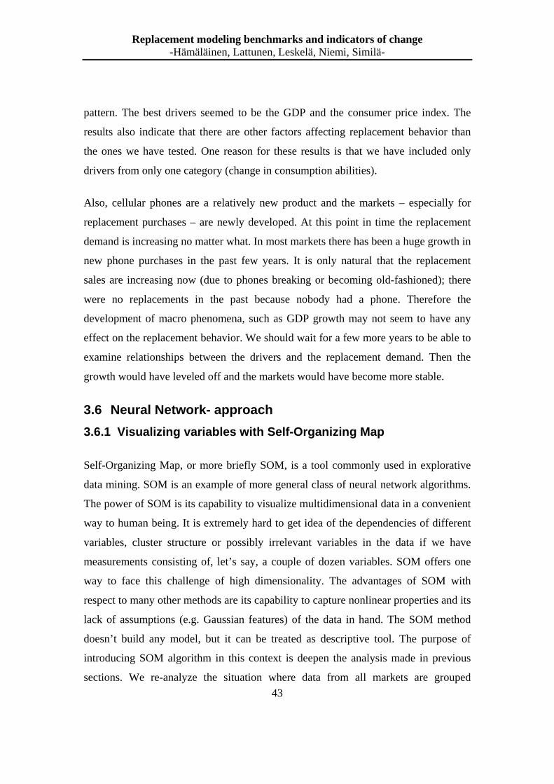
43
pattern. The best drivers seemed to be the GDP and the consumer price index. The
results also indicate that there are other factors affecting replacement behavior than
the ones we have tested. One reason for these results is that we have included only
drivers from only one category (change in consumption abilities).
Also, cellular phones are a relatively new product and the markets – especially for
replacement purchases – are newly developed. At this point in time the replacement
demand is increasing no matter what. In most markets there has been a huge growth in
new phone purchases in the past few years. It is only natural that the replacement
sales are increasing now (due to phones breaking or becoming old-fashioned); there
were no replacements in the past because nobody had a phone. Therefore the
development of macro phenomena, such as GDP growth may not seem to have any
effect on the replacement behavior. We should wait for a few more years to be able to
examine relationships between the drivers and the replacement demand. Then the
growth would have leveled off and the markets would have become more stable.
3.6 Neural Network- approach
3.6.1 Visualizing variables with Self-Organizing Ma p
Self-Organizing Map, or more briefly SOM, is a tool commonly used in explorative
data mining. SOM is an example of more general class of neural network algorithms.
The power of SOM is its capability to visualize multidimensional data in a convenient
way to human being. It is extremely hard to get idea of the dependencies of different
variables, cluster structure or possibly irrelevant variables in the data if we have
measurements consisting of, let’s say, a couple of dozen variables. SOM offers one
way to face this challenge of high dimensionality. The advantages of SOM with
respect to many other methods are its capability to capture nonlinear properties and its
lack of assumptions (e.g. Gaussian features) of the data in hand. The SOM method
doesn’t build any model, but it can be treated as descriptive tool. The purpose of
introducing SOM algorithm in this context is deepen the analysis made in previous
sections. We re-analyze the situation where data from all markets are grouped

Replacement modeling benchmarks and indicators of change -Hämäläinen, Lattunen, Leskelä, Niemi, Similä-
44
together and find possible explanations to small linear correlations reported in Table
8. The SOM method suits best in situations where the amount of observations in data
is high, so analysis of the individual markets is excluded.
Overview of the SOM method
A brief overview of the SOM algorithm will be given next. For a more detail
description, we encourage to familiarize oneself with the book by Kohonen (1997).
SOM consists of a certain number of neurons. The number of neurons can be freely
chosen, but in practice the dimensionality of the data and the wanted abstraction level
fix this amount. Each neuron has got a position in the data space spanned by the
variables of the data. We call this space input data space. At the very beginning, the
positions of the neurons are randomized. The SOM algorithm tries to organize the
positions of the neurons to match the probability density of the data. This means that
there are more neurons in those parts of input space where the number of observations
is also high. The neuron map will be loose in the parts of the input space where the
existence of observations is rare. The trained SOM map can thus be interpreted as an
abstraction of the primary data. It is a collection of points in the input data space, the
number of these points is lower than the number of observations in the primary data
and these points try to represent the whole collection of primary data observations.
An important property of SOM map is the fact that for each of the neurons, the
neighboring neighbors are specified. Although the positions of the neurons are
randomized at the beginning of the training procedure, the neighboring neurons are
close to each other after the training has been completed. This is the explanation for
the name self-organizing. The neighborhood preserving property of SOM makes it
possibly to arrange the neurons on a discrete grid revealing the neighboring
connections between the neurons. Here we restrict to the situation, where each neuron
has six neighbors and the resulting SOM grid becomes hexagonal. We call the
discrete grid as output data space. As earlier stated, each neuron has got a position in
the continuous input data space. Now the neurons can also be placed on the discrete
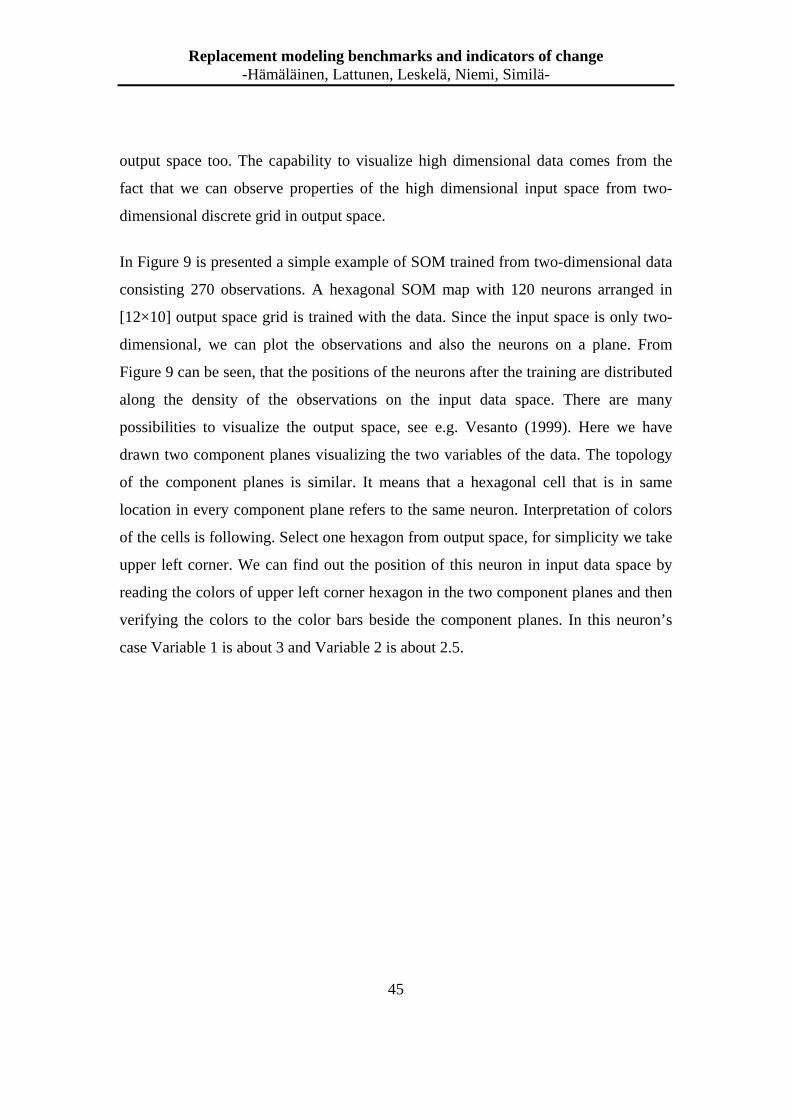
Replacement modeling benchmarks and indicators of change -Hämäläinen, Lattunen, Leskelä, Niemi, Similä-
45
output space too. The capability to visualize high dimensional data comes from the
fact that we can observe properties of the high dimensional input space from two-
dimensional discrete grid in output space.
In Figure 9 is presented a simple example of SOM trained from two-dimensional data
consisting 270 observations. A hexagonal SOM map with 120 neurons arranged in
[12×10] output space grid is trained with the data. Since the input space is only two-
dimensional, we can plot the observations and also the neurons on a plane. From
Figure 9 can be seen, that the positions of the neurons after the training are distributed
along the density of the observations on the input data space. There are many
possibilities to visualize the output space, see e.g. Vesanto (1999). Here we have
drawn two component planes visualizing the two variables of the data. The topology
of the component planes is similar. It means that a hexagonal cell that is in same
location in every component plane refers to the same neuron. Interpretation of colors
of the cells is following. Select one hexagon from output space, for simplicity we take
upper left corner. We can find out the position of this neuron in input data space by
reading the colors of upper left corner hexagon in the two component planes and then
verifying the colors to the color bars beside the component planes. In this neuron’s
case Variable 1 is about 3 and Variable 2 is about 2.5.

Replacement modeling benchmarks and indicators of change -Hämäläinen, Lattunen, Leskelä, Niemi, Similä-
46
Figure 9 Example of SOM trained from two-dimensional data. On the upper left subfigure are
plotted the observations from the data. The lower left figure shows the organized SOM neurons
and connections between them in the primary data space. The subfigures on the right hand side
are SOM component planes in the discrete output grid.
Applying SOM method to the data
In the previous sections we calculated linear correlations (Table 8) and built linear
regression models (Table 9). Pair-wise linear correlations are very small and linear
regression model is extremely sensitive to missing values as stated earlier. These facts
encouraged us to make some reanalysis with different type of method. SOM suits well

Replacement modeling benchmarks and indicators of change -Hämäläinen, Lattunen, Leskelä, Niemi, Similä-
47
in this purpose, since it truly differs from the methods applied earlier. Nonlinear
dependencies between the dependent and explanatory variables weren’t earlier taken
into account and the found correlation results with t-values may be doubtful because
normality of the data cannot be assumed.
The training data for SOM consists of quarterly observations from 10 market areas
over the total available time period. The markets were aggregated into one matrix
containing total 270 observations. Market 3 was again excluded because the lack of
most values. One observation was lost from each market since the presence of a
variable derived from one year lagged values. The resulting SOM is presented in
Figure 10 and the variables included in the training can be found on the top of the
component planes. Interpretation of the map is harder than usually, because the values
of most variables in the observations are proportions or differences from the reference
quarter defined by the supplier of the data. The reference value is from same year in
every market, but each market has its own value. Thus the results from the SOM map
must be interpreted as market’s deviation from its own reference value. The lack of
knowledge about the absolute values and the preceding manipulations done to the data
makes again the found results doubtful.
The analysis of nonlinear dependencies means seeking such areas from different
component planes that looks someway similar. In Figure 10, there is a strong
correlation between “GDP” and “Wage compensation”. An example of more local
nature of correlation is between “Consumer price index” and “Exchange rate”. The
important thing in our problem context is that there is not preset any single variable or
combination of several variables, which could explain the shape of the component
plane representing the dependent variable, “Replacement per subscribers”. Only the
lowest values of “Long term interest rate” indicate high “Replacement per
subscribers” value. This negative correlation was found earlier during linear
correlation analysis. The SOM training procedure was repeated with some variables
left out, but the situation remained quite same. The SOM based analysis doesn’t thus

Replacement modeling benchmarks and indicators of change -Hämäläinen, Lattunen, Leskelä, Niemi, Similä-
48
reveal any latent properties of regression that the linear analysis might earlier have
unobserved.
Still, the use of SOM method can give valuable information of other properties from
the problem in hand. One way to increase the value of SOM is incorporate the time
behavior of markets in the analysis. SOM is static itself, but if we assume that the
neurons represent the possible “states of the world”, we can analyze changes of
markets’ states in time on the component planes. In Figure 10 is represented the
trajectory of Market 1 starting from the Q2 of 1996 and ending at Q4 of 2002. The
trajectory reveals that the Market 1 has increased the total sales. The increase is at
first sales to new customers and at the latter part of time interval the market is heading
to the high replacement sales area of the map. This example shows how SOM can be
used in monitoring a market’s change in time versus several variables.

Replacement modeling benchmarks and indicators of change -Hämäläinen, Lattunen, Leskelä, Niemi, Similä-
49
Figure 10, SOM component planes representing eleven measured variables. The trajectory
indicating the quarterly movement of Market 1 (from Q2 of 1996 to Q4 of 2002) is shown on top
of each component plane. The starting point of the trajectory is marked with dot.

Replacement modeling benchmarks and indicators of change -Hämäläinen, Lattunen, Leskelä, Niemi, Similä-
50
4 Conclusions
Replacement demand forecasting provides a formidable challenge in the
telecommunications industry due to its dynamic nature. Many traditional methods are
rendered useless as there does not exists sufficient amounts of time series data and
even if feasible data is found it contains so many discontinuity points that estimation
relying on it will require significant effort.
The contribution and focus of this paper was in introducing different factors that
might be used in estimating replacement parameters. Our analysis showed that Nokia
should clearly focus on parameters from four categories, which were parameters
influencing consumption abilities, price of mobile phones, subsidy levels, and the
overall technological change in the industry. We believe that through these parameters
Nokia could accurately estimate, for example, the average life cycle of mobile phones
and so use some of the models found in the literature search.
We also conducted an example analysis with data from Nokia’s sources. The idea was
to test how we could estimate replacement sales parameters in the consumption
abilities category. The analysis shows that there exists a correlation between
replacement sales and different parameters like GDP, consumer price index and retail
sales. However, these relations are individual for each market and differ a lot between
markets. This could be due to the fact that the markets are in different phases of
economic development. One can expect industrialized countries to behave differently
from developing countries. Also, an economic crisis in a country can affect the
behavior of the drivers in the market.
From the correlation and regression analyses, as well as the SOM approach we can
conclude that models would be better built for each individual market rather than
trying to group all the markets together. There are some drivers among those that we
tested that would seem to explain changes in the replacement pattern. However, we
have tested drivers from only one category (changes in consumption abilities) out of

Replacement modeling benchmarks and indicators of change -Hämäläinen, Lattunen, Leskelä, Niemi, Similä-
51
four. The next step would be to add drivers from the other three categories as well.
This would be a good topic for future research into the replacement pattern of cellular
phones. The data for the three other categories is more difficult to obtain. Especially
the measurement of technological change is difficult. One point of interest in the
future would be to construct a technology index as a proxy for technological change.

Replacement modeling benchmarks and indicators of change -Hämäläinen, Lattunen, Leskelä, Niemi, Similä-
52
5 References
Ben-Akiva, Moshe, and Lerman, Steven R., 1985, “Discrete Choice Analysis: Theory
and Applications to Travel Demand”, MIT Press, Cambridge, MA.
Duk Bin Jun, Yoon S. Park, 1999, “A Choice-Based Diffusion Model for Multiple
Generations of Products”, Technological Forecasting and Social Change, Vol. 61, pp.
45-58.
Fernandez, V.P., 2001, ”Observable and Unobservable Determinants of Replacement
of Home Appliances”, Energy Economics, Vol. 23, pp. 305-323.
Islam, T., and Meade, N., 2000, “Modelling diffusion and replacement”, European
Journal of Operational Research, Vol. 125, pp. 551-570.
Kiefer, N.M, 1988, “Economic Duration Data and Hazard Functions”, Journal of
Economic Literature, Vol. 26, pp.646-679.
Kohonen, T., 1997, “Self-Organizing Maps, Series in Information Sciences”, second
ed., Springer.
Lancaster, T., 1979, “Econometric Methods for the Duration of Unemployment”,
Econometrica, Vol. 47, pp. 939-956.
Marell A, Davidson P, and Gärling T, 1995, “Environmentally friendly replacement
of automobiles”, Journal of economic psychology, Vol. 16, pp. 513-529.
Raymond, J.E., Beard, T.R., and Gropper, D.M., 1993, “Modelling the Consumer’s
decision to replace durable goods: A Hazard Function Approach”, Applied
Economics, Vol. 25, pp. 1287-1293.
Simon, H.A., 1955, “A behavioral model of rational choice”, Quarterly Journal of
Economics, Vol. 69, pp. 99-118.

Replacement modeling benchmarks and indicators of change -Hämäläinen, Lattunen, Leskelä, Niemi, Similä-
53
Simon, H.A., 1956, “Rational choice and the structure of the environment”,
Psychological Review, Vol. 63, pp. 129-138.
Vesanto J., 1999, “SOM-Based Data Visualization Methods”, Intelligent Data
Analysis, Vol. 3.

Replacement modeling benchmarks and indicators of change -Hämäläinen, Lattunen, Leskelä, Niemi, Similä-
54
Appendices
5.1 Appendix 1 – Correlations
Correlations with replacements per subscribers, all marketsVariable Correlation p-value Cases included Missing cases
Consumer confidence 0,028 0,713 175 105Consumer price index 0,171 0,005 270 10Exchange rate 0,067 0,272 270 10GDP 0,212 0,001 270 10Long term interest rate -0,695 0,000 140 140Retail sales 0,275 0,000 189 91Short term interest rate -0,388 0,000 216 64Subsidy level 0,319 0,000 198 82Wage compensation 0,317 0,000 158 122
Correlations with replacements per subscribers, Market 1Variable Correlation p-value Cases included Missing cases
Consumer confidence -0,510 0,007 27 1Consumer price index 0,901 0,000 27 1Exchange rate N/AGDP 0,893 0,000 27 1Long term interest rate -0,569 0,002 27 1Retail sales 0,931 0,000 27 1Short term interest rate -0,682 0,000 27 1Subsidy level N/AWage compensation 0,892 0,000 27 1
Correlations with replacements per subscribers, Market 2Variable Correlation p-value Cases included Missing cases
Consumer confidence 0,0126 0,9643 15 13Consumer price index -0,4407 0,0214 27 1Exchange rate -0,2523 0,2042 27 1GDP 0,6771 0,0001 27 1Long term interest rate N/ARetail sales 0,6124 0,0007 27 1Short term interest rate N/ASubsidy level 0,3581 0,0038 27 1Wage compensation 0,4193 0,0464 23 5

Replacement modeling benchmarks and indicators of change -Hämäläinen, Lattunen, Leskelä, Niemi, Similä-
55
Correlations with replacements per subscribers, Market 4Variable Correlation p-value Cases included Missing cases
Consumer confidence -0,029 0,888 27 1Consumer price index 0,885 0,000 27 1Exchange rate 0,712 0,000 27 1GDP 0,790 0,000 27 1Long term interest rate -0,266 0,179 27 1Retail sales 0,864 0,000 27 1Short term interest rate 0,001 0,996 27 1Subsidy level N/A 28Wage compensation 0,887 0,000 27 1
Correlations with replacements per subscribers, Market 5Variable Correlation p-value Cases included Missing cases
Consumer confidence -0,206 0,300 27 1Consumer price index 0,619 0,001 27 1Exchange rate 0,568 0,002 27 1GDP 0,645 0,000 27 1Long term interest rate -0,705 0,000 27 1Retail sales 0,737 0,000 27 1Short term interest rate -0,821 0,000 27 1Subsidy level N/AWage compensation 0,536 0,004 27 1
Correlations with replacements per subscribers, Market 6Variable Correlation p-value Cases included Missing cases
Consumer confidence -0,084 0,676 27 1Consumer price index 0,405 0,036 27 1Exchange rate 0,313 0,112 27 1GDP 0,286 0,149 27 1Long term interest rate 0,026 0,937 12 16Retail sales N/AShort term interest rate -0,450 0,019 27 1Subsidy level 0,426 0,027 27 1Wage compensation 0,351 0,073 27 1

Replacement modeling benchmarks and indicators of change -Hämäläinen, Lattunen, Leskelä, Niemi, Similä-
56
Correlations with replacements per subscribers, Market 7Variable Correlation p-value Cases included Missing cases
Consumer confidence 0,061 0,764 27 1Consumer price index 0,095 0,638 27 1Exchange rate 0,009 0,966 27 1GDP 0,472 0,013 27 1Long term interest rate -0,754 0,000 27 1Retail sales -0,692 0,000 27 1Short term interest rate -0,488 0,010 27 1Subsidy level -0,094 0,640 27 1Wage compensation -0,148 0,460 27 1
Correlations with replacements per subscribers, Market 8Variable Correlation p-value Cases included Missing cases
Consumer confidence 0,109 0,604 25 3Consumer price index 0,287 0,147 27 1Exchange rate 0,644 0,000 27 1GDP -0,536 0,004 27 1Long term interest rate 0,683 0,001 27 1Retail sales 0,052 0,795 27 1Short term interest rate 0,013 0,947 27 1Subsidy level N/A 27 1Wage compensation N/A 27 1
Correlations with replacements per subscribers, Market 9Variable Correlation p-value Cases included Missing cases
Consumer confidence N/AConsumer price index -0,473 0,013 27 1Exchange rate -0,477 0,012 27 1GDP 0,242 0,223 27 1Long term interest rate N/A 27 1Retail sales N/A 27 1Short term interest rate -0,135 0,502 27 1Subsidy level N/A 27 1Wage compensation N/A 27 1

Replacement modeling benchmarks and indicators of change -Hämäläinen, Lattunen, Leskelä, Niemi, Similä-
57
Correlations with replacements per subscribers, Market 10Variable Correlation p-value Cases included Missing cases
Consumer confidence N/AConsumer price index -0,346 0,077 27 1Exchange rate -0,455 0,017 27 1GDP -0,353 0,071 27 1Long term interest rate N/A 28Retail sales N/A 28Short term interest rate -0,200 0,920 27 1Subsidy level N/A 28Wage compensation N/A 28
Correlations with replacements per subscribers, Market 11Variable Correlation p-value Cases included Missing cases
Consumer confidence N/A 280Consumer price index -0,62 0,00 27 1Exchange rate 0,79 0,00 27 1GDP 0,60 0,00 27 1Long term interest rate N/A 28Retail sales -0,80 0,00 27 1Short term interest rate N/A 28Subsidy level -0,08 0,68 27 1Wage compensation N/A 28
5.2 Appendix 2 - Project
This chapter will introduce how the actual project was conducted, what were the
different phases and what went well and what could have been done better.
5.2.1 Phases
The project was divided into three major phases, which were the theory phase, the
application phase, and the recommendations and writing phase.

Replacement modeling benchmarks and indicators of change -Hämäläinen, Lattunen, Leskelä, Niemi, Similä-
58
5.2.1.1 Phase 1 – Theory
In the theory phase we conducted a literature research. This was done by searching
different articles from databases and company websites and finally building a
portfolio of feasible papers. It was found that articles on replacement demand
forecasting were few and only four relevant studies were found.
The findings were discussed within the group and presented to the client. Based on
these discussions the plans were refined and the project was ready to move into phase
two.
5.2.1.2 Phase 2 - Application
Phase 2 consisted of multiple different subproblems. First we had to familiarize
ourselves with Nokia’s current model used in replacement forecasting. This was done
with the help of manuals and the actual model.
After spending some time with the current model it was decided that it should not be
emphasized, as new ways of doing things should be introduced. Also the articles
proved to be pretty much useless to our purposes, as they provided only few feasible
ideas and the data available to us did not fill the required criteria.
The emphasis was then shifted to introducing new drivers, which Nokia could use in
estimating parameters for their current model. To do this we analyzed other market
data received from Nokia against historical replacement numbers. We also tried to
apply some new analyzing methods like self-organizing maps so that the data could be
looked at more thoroughly.
5.2.1.3 Phase 3 – Recommendations and writing
In the final phase recommendations for the client were done and the final report was
written. The findings were also discussed with the client in detail.

Replacement modeling benchmarks and indicators of change -Hämäläinen, Lattunen, Leskelä, Niemi, Similä-
59
5.2.2 Workload
The workload experienced during the course is introduced in detail in Table 12. As
one can see, the hours exceeded the hours projected for the course.
The first phase went according to our initial schedule and a theory base of four
different approaches was identified. The second phase, however, exceeded our initial
time projections. Here getting to know the data and analyzing it took far beyond time
that we had estimated and proved to be a real problem with ever changing data. In the
end, phase 3 went according to our plans, as it mostly consisted of writing our results
on paper and discussing them with the client. The project took a little bit longer than
expected. Especially, the analysis of the data and the discussion of the results
exceeded the time allocated for them. However, the actual writing of the report was
faster than we anticipated.

Replacement modeling benchmarks and indicators of change -Hämäläinen, Lattunen, Leskelä, Niemi, Similä-
60
Table 12, The course workload (per person)
Hours Phase 1 Meeting client 3 Article search 5 Reading the articles 10 Compiling results 10
Writing the plan and presenting it 4
Total 32 Phase 2 Getting to know the model 5 Data Getting familiar with data 15 Analyzing 20 Meeting with clients 4 Writing the report 5 Excursions 5 Total 54 Phase 3 Further analysis 15
Developing recommendations 10
Writing the paper 15
Communicating results to client 4
Attending seminar sessions 2 Total 46 Total duration of project 132

Replacement modeling benchmarks and indicators of change -Hämäläinen, Lattunen, Leskelä, Niemi, Similä-
61
5.2.3 Lessons learned
In many ways, one could say that the project was successful and did not contain any
major failures.
First of all, the project was conducted on time and according to client wishes,
secondly we were able to fulfill our research problem at least in some form. During
the project our team functioned well.
On the other hand, some things could have been done better. In the beginning the
goals were too ambitious as we desired to test new models with Nokia’s data and
thereby introduce new ways of conducting forecasts. However, this proved not to be
the case as it was not possible to apply the models directly to the available data. Also,
when defining the project scope we could have identified a clear, realizable goal. The
scope of the project changed during the course of the semester, so we had to spend
additional time refiguring the specifications. However, things like these are hard to
foresee and from our perspective we managed the project fine