‘Mobile’izing Agricultural Advice: Technology Adoption, Diffusion and Sustainability

Shawn A. Cole A. Nilesh Fernando

Working Paper 13-047

Working Paper 13-047

Copyright © 2012, 2016 by Shawn A. Cole and A. Nilesh Fernando

Working papers are in draft form. This working paper is distributed for purposes of comment and discussion only. It may not be reproduced without permission of the copyright holder. Copies of working papers are available from the author.

‘Mobile’izing Agricultural Advice: Technology Adoption, Diffusion and Sustainability

Shawn A. Cole Harvard Business School

A. Nilesh Fernando Harvard University

‘Mobile’izing Agricultural Advice: Technology Adoption,

Di↵usion and Sustainability ⇤

Shawn A. Cole and A. Nilesh Fernando †

April 29, 2016

Abstract

We examine the role of management in agricultural productivity, by evaluating a mobile-phone based

agricultural advice service provided to farmers in India. Demand for advice is high; and advice changes

practices, increasing yields in cumin (28%) and cotton (8.6%, for a sub-group receiving reminders). Informa-

tion spreads, as non-treated farmers with more treated peers change practices and lose less to pest attacks.

Though willingness to pay for the service is low, the value of the information externality exceeds the subsidy

that would be necessary to operate the service. We estimate each dollar spent on the service yields a $10

private return.

JEL Classification Numbers: O12, O13, Q16

Keywords: Technology Adoption, Agricultural Extension, Informational Ine�ciencies

⇤This paper was previously circulated as ‘The Value of Advice: Evidence from the Adoption of Agricul-tural Practices’

†Harvard Business School (scole@hbs.edu) and Harvard University (afernando@fas.harvard.edu). Thisresearch was funded by research grants from USAID and AusAID; Cole also acknowledges support from theDivision of Faculty Research and Development at Harvard Business School. Fernando acknowledges supportfrom the HKS Sustainability Science program. In 2015, Cole co-founded a non-profit organization seekingto further test, and bring to scale, mobile-phone based agricultural advice services; this non-profit fundeda post-doctoral position for Fernando. We thank the Development Support Centre (DSC) in Ahmedabadand especially Paresh Dave, Natubhai Makwana and Sachin Oza for their assistance and cooperation. Ad-ditionally, we thank Neil Patel and Awaaz.De for hosting the AO system and the Centre for Micro Finance(CMF), Chennai and Shahid Vaziralli for support in administering the evaluation. We thank Niharika Singh,Niriksha Shetty, Ishani Desai, Tanaya Devi and HK Seo for excellent research assistance. We are especiallyindebted to Tarun Pokiya for suggestions, his agricultural expertise and management of the AO system.This paper has benefited from comments from seminar participants at Harvard, MIT, NEUDC, and IFPRI.

1 Introduction

Agricultural productivity varies dramatically around the world. For example, India is the

second largest producer of cotton in the world, after China. Yet, Indian cotton productivity

ranks 78th in the world, with yields only one-third as large as those in China. While credit

constraints, missing insurance markets, and poor infrastructure may account for some of this

disparity, a variety of observers have pointed out the possibility that suboptimal agricultural

practices may also be to blame (Jack, 2011).

This is not a novel idea. For decades, the Government of India, like most governments

in the developing world, has operated a system of agricultural extension, intended to spread

information on new agricultural practices and technologies, through a large work force of

public extension agents. However, evidence of the e�cacy of these extension services is

quite limited. In India, dispersed rural populations, monitoring di�culties and a lack of

accountability hamper the e�cacy of traditional extension systems: fewer than 6% of the

agricultural population reports having received information from these services.1

This paper examines whether the introduction of a low-cost information and communi-

cations technology (ICT), able to deliver timely, relevant, and actionable information and

advice to farmers at dramatically lower cost than any traditional service can improve agri-

cultural management. We evaluate Avaaj Otalo (AO), a mobile phone-based technology

that allows farmers to call a hotline, ask questions and receive responses from agricultural

scientists and local extension workers. Callers can also listen to answers to questions posed

by other farmers.

Working with the Development Support Centre (DSC), an NGO with extensive experi-

ence in delivering agricultural extension, the research team randomly assigned toll-free access

to AO to 800 households; half of this group was o↵ered an annual traditional extension ses-

sion to complement the AO service; a further 400 households served as a control group. The

households were spread across 40 villages in Surendranagar district in Gujarat, India, and

randomization occurred at the household level.

The AO service also included weekly push content, delivering time-sensitive informa-

tion such as weather forecasts and pest planning strategies directly to farmers. This paper

presents the results using three rounds of household surveys: a baseline, a midline one year

later, and an endline two years after the study began. To capture information spillovers, all

respondents at baseline were asked to identify individuals with whom they discussed farming:

1This estimate is from the 59th round of the National Sample Survey (NSS) and asks farmers abouttheir information sources for ‘modern agricultural technologies’. See Glendenning et al., 2010 for a detaileddiscussion of this data.

1

we surveyed this peer group by phone in May-November of 2012.

Demand for agricultural information is substantial: more than 80% of the treatment

group called into the AO line over two years. The average treatment respondent made

20 calls and used the service for more than 2.5 hours. We show that AO had a range of

important, positive e↵ects on farmer behavior. It significantly changed farmers’ sources

of information for sowing and input-related decisions. In particular, farmers relied less on

commissions-motivated agricultural input dealers for pesticide advice and less on their prior

experience for fertilizer-related decisions. Instead, farmers dramatically increase their usage

of and trust in mobile phone-based information across a number of agricultural decisions.

Importantly, treated farmers were significantly more likely to adopt agricultural practices

and inputs recommended by the service. These inputs choices include recommended seed

varieties, fertilizers, pesticides and irrigation practices. While yields are often di�cult to

measure, we do find evidence of improvements here as well: treatment e↵ects up to 8.6%

higher for cotton, and 28.0% higher for cumin.

Our treatment also induces variation in information available in social networks, allowing

us to estimate peer e↵ects. We find that individuals with more treated peers (social network

members) plant more cumin and report lower pest-related cotton losses. In addition, treated

respondents with treated peers are more likely to adopt pest management recommendations

for cotton.

Following the endline, we conduct a series of willingness to pay experiments to estimate

demand for AO. Average willingness to pay for a 9-month AO subscription across multiple

price elicitation methods is roughly $2, compared to a cost of provision of for the same period

of $7. This implies a $12 subsidy per farmer to run the service over two years. In support

of such a subsidy, we estimate that each dollar invested in AO generates a return of more

than $10, with the return for a two-year subscription at more than $200. Moreover, we find

that a conservative estimate of the positive externality created by a treated farmer is more

than 2 times the subsidy needed to cover operational costs.

First, this paper contributes to an understanding of the mechanisms underlying the

dramatic variation in the productivity of firms and farms in developing countries, and the

role of management practices in improving productivity. These large productivity di↵erences

have in part motivated the recent literature on non-aggregative growth (Banerjee and Duflo,

2005; Hsieh and Klenow, 2009). While a large literature focuses on the microeconomics of

technology adoption (for a survey, see Foster and Rosenzweig, 2010), we instead focus on

whether a consulting-like service can facilitate improved production practices. (Duflo et al.,

2011.) Our treatments di↵er from much previous work in this space in that participants

receive a continuous flow of demand-oriented information, rather than a one-o↵ provision of

2

supply-driven information. See McKenzie and Woodru↵, 2012 for a discussion of training

and consulting evidence for small firms in developing countries.

More specifically, this paper advances the literature on the e�cacy of agricultural exten-

sion (Feder et al., 1987; Gandhi et al., 2009; Duflo et al., 2011). The existing literature finds

mixed evidence of e�cacy, though it is not clear whether this is due to variation in programs

o↵ered, or methodological challenges associated with evaluating programs without plausibly

exogenous variation (Birkhaeuser et al., 1991). This paper complements recent evidence on

the historical e�cacy of agricultural extension in promoting the adoption of new agricul-

tural technologies in India (Bardhan and Mookherjee, 2011), and provides guidance as to

lower-cost solutions for delivering advice. To our knowledge, our study is the first rigorous

evaluation of mobile phone-based extension and, more generally, the first evaluation of a

demand-driven extension service delivered by any means. BenYishay and Mobarak (2013)

compare the impact of incentivized extension agents to non-incentivized extension agents in

Malawi.

We demonstrate that informational ine�ciencies are real and farmers are aware they

lack information: there is considerable demand for high-quality agricultural information2.

Perhaps most importantly, we demonstrate that ICTs can lead to productivity gains in an

industry that is both important–agriculture in the primary activity of the 47% of the world

living in rural areas–and historically virtually unreliant on ICTs. Our results complement

recent work that measures productivity-enhanancement from ICTs in developed countries

(Draca et al., 2006).

We provide some evidence of the existence of a “digital divide,” as richer individuals

are more likely to use the service and adopt recommended practices for cotton cultivation.

This is true even though the treatment group is relatively homogeneous, and even though

the technology was delivered for free, and specifically designed to be accessible to a poor,

illiterate population.

Finally, we make a methodological and an empirical contribution related to measuring

demand and understanding welfare among di↵erent price regimes. First, we measure will-

ingness to pay, using two di↵erent methodologies, in a real-world setting, providing one of

the first large-scale, high-stakes demonstrations that the Becker-DeGroot-Marschak (BDM)

mechanism can be e↵ective. Second, using the demand curve estimated with the BDM

method, we find that a 91% subsidy induces nearly 20 times the social benefit as pricing

just above marginal cost. This latter finding supports the role of subsidies in promoting the

adoption of an agricultural technology in a manner similar to Cohen et al. (2010).

2Informational ine�ciencies in the context of technology adoption have been defined as a situation inwhich farmers may not be aware of new agricultural technologies, or how they should be utilized (Jack,2011)

3

This paper is organized as follows. The next section provides context and the details of

the AO intervention. Section 3 presents the experimental design and the empirical strategy,

while Section 4 presents the results from the two years of survey data. Following this, Section

5 considers threats to the validity of the results, and Section 6 concludes.

2 Context and Intervention Description

2.1 Agricultural Extension

According to the World Bank, there are more than 1 million agricultural extension workers

in developing countries, and public agencies have spent over $10 billion dollars on pub-

lic extension programs in the past five decades (Feder, 2005). The traditional extension

model, “Training and Visit” extension, has been promoted by the World Bank through-

out the developing world and is generally characterized by government-employed extension

agents visiting farmers individually or in groups to demonstrate agricultural best practices

(Anderson and Birner, 2007). Like many developing countries, India has a system of local

agricultural research universities and district level extension centers, producing a wealth of

specific knowledge. In 2010, the Government of India spent $300 million on agricultural

research, and a further $60 million on public extension programs (RBI, 2010).

Yet, traditional extension faces several important challenges that limit its e�cacy.

Spatial Dimension: Limited transportation infrastructure in rural areas and the high costs of

delivering information in person greatly limit the reach of extension programs. The problem

is particularly acute in interior villages in India, where farmers often live in houses adjacent

to their plots during the agricultural cycle, creating a barrier to both the delivery and receipt

of information.

Temporal Dimension: As agricultural extension is rarely provided to farmers on a re-

curring basis, the inability of farmers to follow-up on information delivered may limit their

willingness to adopt new technologies. Infrequent and irregular meetings limit the ability to

provide timely information, such as how to adapt to inclement weather or unfamiliar pest

infestations.

Institutional Rigidities : In the developing world, government service providers often face

institutional di�culties. The reliance on extension agents to deliver in-person information is

subject to general monitoring problems in a principal-agent framework (Anderson and Feder,

2007). For example, monthly performance quotas lead agents to target the easiest-to-reach

farmers, and rarely exceed targets. Political capture may also lead agents to focus outreach

on groups a�liated with the local government, rather than to marginalized groups for whom

4

the incremental benefit may be higher. Even when an extension agent reaches farmers, the

information delivered must be locally relevant, and delivered in a manner that is accessible

to farmers with low levels of literacy.

The importance of these constraints is di�cult to overstate (Birkhaeuser et al., 1991;

Saito and Weidemann, 1990.) A recent nationally representative survey shows that just 5.7%

of farmers report receiving information about modern agricultural technologies from public

extension agents in India (Glendenning et al., 2010.) This failure is only partly attributable

to the misaligned incentives of agricultural extension workers; more fundamentally, it is

attributable to the high cost of reaching farmers in interior rural areas.

Finally, a potential problem is that information provision to farmers is often “top-down.”

This may result in an inadequate diagnosis of the di�culties currently facing farmers, as well

as information that is often too technical for semi-literate farming populations. This problem

may a↵ect adoption of new technologies as well as optimal use of current technologies.

In the absence of expert advice, farmers seek out agricultural information through word

of mouth, generic broadcast programming, or agricultural input dealers, who may be poorly

informed or face incentives to recommend the wrong product or excessive dosage (Anderson

and Birner, 2007).3

These di�culties combine to limit the reliable flow of information from agricultural re-

search universities to farmers, and may limit their awareness of and willingness to adopt

new agricultural technologies. Overcoming these “informational ine�ciencies” may there-

fore dramatically improve agricultural productivity and farmer welfare. The emergence of

mobile phone networks and the rapid growth of mobile phone ownership across South Asia

and Sub-Saharan Africa has opened up the possibility of using a completely di↵erent model

in delivering agricultural extension services.

2.2 Avaaj Otalo: Mobile Phone-Based Extension

Roughly 50% of the Indian labor force, or 250 million people, are engaged in agriculture. As

approximately 48% own a mobile phone (as of 2015), mobile phone-based extension could

serve as many as 120 million farmers nationally 4. Mobile phone access has fundamentally

3An audit study of 36 input dealerships in a block near our study site provides a measure of the qualityof advice provided by commissions-motivated input dealers. The findings suggest that the informationprovided is rarely customized to specific pest management problems of the farmer, and often takes the formof ine↵ective pesticides that were traditionally useful, but are no longer e↵ective against the dominant classof pests that a✏ict cotton cultivation.

4These figures are calculated using the Annual Report of the Telecom Regulatory Authority of India(India, 2015) and the World Bank Development Indicators (Group, 2012). The WDI estimates the ruralpopulation of India at 876 million while the TRAI estimates the number of subscriptions in rural India at423 million. In addition the WDI estimate that 50% of the workforce are engaged in agriculture of a totalworkforce of 497 million

5

changed the way people communicate with each other, and has increased information flows

across the country’s diverse geographic areas. As coverage continues to expand in rural areas,

mobile phones carry enormous promise as a means for delivering extension to the country’s

numerous small and marginal farmers (Aker, 2011).

Our intervention utilizes an innovative information technology service, Avaaj Otalo (AO).

AO uses an open-source platform to deliver information by phone. Information can be

delivered to and shared by farmers. Farmers receive weekly push-content, which includes

detailed agricultural information on weather and crop conditions that are delivered through

an automated voice message.

Farmers can also call into a toll-free hotline that connects them to the AO platform and

ask questions on a variety of agricultural topics of interest to them. Sta↵ agronomists at the

Development Support Centre (DSC) – our field partner – with experience in local agricultural

practices receive these requests and deliver customized advice to these farmers, via recorded

voice messages. Farmers may also listen and respond to the questions their peers ask on the

AO platform, which is moderated by DSC. The AO interface features a touch-tone navigation

system with local language prompts, developed specifically for ease of use by semi-literate

farmers. The platform, which has now been deployed in a range of domains, was initially

developed as part of a Berkeley-Stanford research project on human-computer interaction,

in cooperation with the DSC in rural Gujarat (Patel et al., 2010).

Mobile phone-based extension allows us to tackle many problems associated with tra-

ditional extension. AO has the capability to reach millions of previously excluded farmers

at a virtually negligible marginal cost. Farmers in isolated villages can request and receive

information from AO at any point during the agricultural season, something they are typi-

cally unable to do under traditional extension. Farmers receive calls with potentially useful

agricultural information on their mobile phones, and need not leave their fields to access the

information. In case a farmer misses a call, she can call back and listen to that information

on the main line. AO thus largely solves the spatial problems of extension delivery discussed

earlier.

A considerable innovation of AO is tackling the temporal problem of extension delivery.

The agricultural cycle can be subject to unanticipated shocks such as weather irregularities

and pest attacks, both of which require swift responses to minimize damage to a standing

crop. Because farmers can call in and ask questions as frequently as they want, they can

get updated and timely information on how to deal with these unanticipated shocks. This

functionality may increase the risk-bearing capacity of farmers by empowering them with

access to consistent and quality advice.

With respect to problems of an institutional nature mentioned earlier, AO facilitates

6

precise and low-cost monitoring. The computer platform allows easy audits of answers that

sta↵ agronomists o↵er, greatly limiting the agency problem. Additionally, the AO system

allows for demand-driven extension, increasing the likelihood that the information is relevant

and useful to farmers. Push-content is developed by polling a random set of farmers each

week to elicit a representative set of concerns. In addition to this polling, the questions asked

by calling into AO also provide the information provider a sense of farmers’ contemporaneous

concerns. This practice of demand-oriented information provision should improve both the

allocation and the likelihood of utilization of the information.

However, while AO overcomes many of the challenges of traditional extension, it elim-

inates in-person demonstrations, which may be a particularly e↵ective way of conveying

information about agricultural practices. As discussed in the following section, our study

design allows us to estimate the extent to which in-person extension serves as a complement

to AO-based extension, by providing a subset of farmers with both traditional extension

administered through sta↵ at DSC and toll-free access to AO.

3 Experimental Design & Empirical Strategy

Two administrative blocks5, Chotila and Sayla, in the Surendranagar district of Gujarat

were chosen as the site of the study, as our field partner, DSC, had done work in the area.

Farmers lists, consisting of all households which expressed willingness to participate, grew

cotton, and owned a mobile phone, were created in 40 villages, and served as our sampling

frame.

A sample of 1,200 respondents was selected at random from this pool, with 30 households

in each village participating in the study. Figure 1 summarizes the experimental design used

in this study. Treatments were randomly assigned at the household-level using a scratch-card

lottery. The sample was split into three equal groups. The first treatment group (hereafter,

AOE) received toll-free access to AO in addition to traditional extension. The traditional

extension component consisted of a single session each year lasting roughly two-and-a-half

hours on DSC premises in Surendranagar. The second treatment group (hereafter, AO)

received toll-free access to AO, but no o↵er of traditional agricultural extension, and the final

set of households served as the control group. In addition, among the two treatment groups

(AO and AOE), 500 were randomly selected to receive bi-weekly reminder calls (hereafter,

reminder group) to use the service while the remaining 300 did not.

Figure 2 provides a timeline for the study. Baseline data was collected in June and July,

5A block is an administrative unit below the district level

7

2011, and a phone survey consisting of 798 respondents was completed in November 2011.6

The midline survey was completed by August 2012, and the endline survey was completed

by August 2013.

To gauge balance and describe our first stage, we compute a simple di↵erence specification

of the form:

yiv = ↵v + �1 Treativ + "i (1)

where, ↵v is a village fixed e↵ect, Treativ is an indicator variable that takes on the value 1

for an individual, i, in village v assigned to a treatment group and 0 for an individual assigned

to the control group. We report robust standard errors below the coe�cient estimates.

Because of random assignment, the causal e↵ect of the intervention can be gauged by

computing a standard di↵erence-in-di↵erence specification:

yivt = ↵v + �1 Treativ + �2 Postt + �3 (Treat ⇤ Post)ivt + "i (2)

where, ↵v and Treativ are as above, Postt is an indicator variable that takes on a value

of 1 if the observation was collected at the endline (or the midline) 0 otherwise, and (Treat⇤Post)ivt is the interaction of the preceding two terms.

In addition, we explore heterogeneity in the treatment e↵ect by interacting the di↵erence-

in-di↵erence specification in Equation (2) with a dummy variable capturing the heterogeneity

of interest:

yivt = ↵v + �1 Treativ + �2 I(Xiv > Median) + �3 Treativ ⇤ I(Xiv > Median)

+�4 Treativ ⇤ Postt + �5 I(Xiv > Median) ⇤ Postt

+�6 Treativ ⇤ I(Xiv > Median) ⇤ Postt + "ivt (3)

where, Xiv is the variable across which we explore heterogeneity in treatment e↵ects, and

I(Xiv > Median) a dummy equal to one when the observation is above the median level of

Xiv.

While dramatically increasing statistical power, the decision to randomize at the house-

hold rather than village level raises the possibility that the control group may also have

6The previous version of this paper (Cole and Fernando, 2012) analyzed treatment e↵ects using resultsfrom this phone survey.

8

access to information through our treatment group. This suggests that any treatment e↵ects

may in fact underestimate the value of the service.7 Our design asked farmers at baseline

to identify peers–to measure spillovers, we subsequently collect information on 1523 peers of

study respondents using a phone survey in March 2012 and November 2012, hereafter the

‘peer survey’.8 This data allows us to estimate whether the treatment also influences the

outcomes of individuals in our study respondents’ social networks. We estimate the extent

of such peer e↵ects or information spillovers with the following specification:

yiv = ↵v + �(# References in Treatment

# References

)iv +7X

i=2

I(# References = i)iv + "iv (4)

where, ↵v is as above,P7

i=2 I(# References = i)iv is a fixed e↵ect for the number of

peers who cite a respondent as a top agricultural contact and (# References in Treatment# References )iv is

the fraction of these respondents who are assigned to treatment.

We did not prepare a pre-analysis plan prior to undertaking the study. This was in part

due to the dynamic nature of the treatment: the service responded to farmer questions, and

ex-ante, it was not always clear which subjects farmers would inquire about. We address

concerns about multiple inference in two ways. First, we use the content generated by farmers,

and by our agronomist, as a broad guide for conducting empirical analysis.9 Second, we

aggregate agricultural practices into indices, following, for example, Kling et al. (2007).

To construct indices, we do the following. The agronomist in our study, Tarun Pokiya,

characterized the full set of agricultural practices that were recommended by the service.

We then aggregate all variables corresponding to recommended practices by calculating a

z-score for each component and then take the average z-score across components. Each

component z-score is computed relative to the control group mean and standard deviation

at baseline. We have compared this to the method that uses ‘seemingly unrelated regression’

which gives slightly di↵erent standard errors and identical point estimates but is virtually

indistinguishable from this method as suggested by Kling et al. (2007).

7In order to control for spillovers, we estimated the main di↵erence-in-di↵erences specification with con-trols for the fraction of a respondent’s social network that was also a part of the study and the fraction thatwas assigned to treatment. These controls leave the main estimates largely unchanged.

8At baseline, we asked all respondents to list the three contacts with whom they most frequently discussedagricultural information and collected their phone numbers. The ‘peer survey’ collected information from allthese contacts. Note, some of these 1523 peers may themselves be study respondents. The analysis largelyfocuses on 1114 non-study peers

9See Appendix Table A1 for details of questions asked by farmers on the AO service and push contentprovided.

9

3.1 Summary Statistics and Balance

In this section we assess balance between the ‘combined treatment’ group (AO + AOE) and

the control group and the subset of the treatment group that receives reminder calls, referred

to as the ‘reminder’ group, and the control group. We do not find many di↵erences in the

separate treatment e↵ects of the AO and AOE groups and the interaction of these treatments

with reminder calls; the exposition of our paper therefore focuses on the ‘combined treatment’

group, as well a the ‘reminder’ group.10

Table 1 contains summary statistics for age, education, income and cultivation patterns

for respondents in the study, using data from a baseline paper survey conducted in July and

August of 2011. Column (1) reports the mean and standard deviation for the control group,

column (2) tests the initial randomization balance between the combined treatment group

and the control group. Finally, column (3) tests the balance between the reminder group

and the control group.

We see that respondents are on average 46 years old and have approximately 4 years

of education. Columns (2) and (3) show that the randomization was largely successful for

both treatment groups across demographic characteristics (Panel B) and indices capturing

information sources, crop-specific and general input use (Panel C). However, an imbalance

exists in the area of cotton planted between the treatment groups and the control group in

2010 but not in 2011 (both periods are prior to treatment).11 The combined treatment group

is also more likely to grow wheat, but this crop is mostly grown for home consumption in

this context.

As cotton is the most important crop in our sample, we take a conservative approach to

the possibility that baseline cotton levels a↵ect subsequent outcomes and include as controls

the area of cotton cultivated in 2010 and its interaction with the ‘Post’ term in both the

di↵erence-in-di↵erence specification (equation (2)), the heterogeneous e↵ects specification

(equation (3)) and peer e↵ects specification (equation (4)).12

10Appendix A2 tests the balance for the AO and AOE group, while Appendix A3 reports treatment e↵ectsseparately for the AO and the AOE group.

11Note, the 2011 figures for wheat and cumin are not reported as they are grown during the Rabi seasonafter the treatment was administered.

12Appendix Table A4 provides a more systematic treatment of balance in our sample. We look for sig-nificant di↵erences in baseline characteristics between the combined treatment group and control, and thereminder group and control respondents. Among the di↵erences computed using the latter specification(examining all 2,295 baseline variables) we find that 0.7% are significantly di↵erence from zero at the 1%level, 4.4% are di↵erent at the 5% level of significance and 9.5% at the 10% level. These results confirmthat the randomization was successful, and that the cotton imbalance is a result of chance rather than anysystematic mistake in the randomization mechanism.

10

4 Experimental Results

Cole and Fernando, 2012 describe initial di↵erences measured seven months after the imple-

mentation of AO. After seven months, take-up among the treated group was high, and

we measured several important changes in agricultural behavior: farmers changed their

information-gathering activity, relying less on peers and more on mobile phone-based ad-

vice; treatment farmers were more likely to adopt more e↵ective pesticides, and reduce

expenditure on hazardous, ine↵ective pesticides; and treated farmers were more likely to

grow cumin. A short-coming of the early evidence was that it was based on interviews, con-

ducted by telephone, of only a sub-sample of study participants. In the sections below, we

describe results after treatment households had been o↵ered the service for two full years

primarily using the di↵erence-in-di↵erences specification in Equation (2).

4.1 First Stage: Take-Up and Usage of AO

Table 2 reports information on take-up and usage (first stage). While control respondents

were not barred from AO usage, only four control respondents called into the AO line by

the midline and a further 25 had called in after two years. As a result, virtually all AO

usage is accounted for by respondents in the treatment group. As of August 2013, two years

after commencement of the service, 88% of the treatment group had called into the AO line,

making an average of 22 calls. This represents a substantial increase from the midline, where

65% of the combined treatment group called in, making an average of 9 calls. The mean

usage for treatment respondents is over 2.5 hours, as compared to 1.3 hours at midline. On

average, treatment respondents have listened to 53% of total push call content (54% of total

push call content was the average at the midline). By the endline, the average number of

questions asked by the treatment group is 1.7, with 9% of the treatment group responding

to a question. Further, columns 4 (midline) and 8 (endline) show that the reminder group

had used the service almost an hour more on average, but were not statistically more likely

to call into the line.

Taken together the results represent substantial induced usage for treatment farmers,

although one-fifth of the treatment group did not use the service. Additionally, these average

e↵ects also mask important temporal patterns shown in Figure 3 which reports average AO

use by month. We see that there was substantial usage across treatment arms during the

first six months after the intervention was administered. Following this period, usage has

been trending down, but with important spikes during sowing times and harvest time. This

figure is suggestive of AO users acquiring a stock of knowledge and supplementing thereafter

with dynamic information needs throughout the season.

11

Appendix Table A1 provides a categorization of the questions asked by treatment re-

spondents during the two years of service. (The categories are not mutually exclusive.)

Unsurprisingly, columns 3 and 4 show that most questions (50%) relate to cotton, and a

majority (54%) focus on pest management and these numbers are relatively stable across

both years. Table A1 also reports information on the content of push calls (columns 5-8),

which tended to provide more information on cumin and wheat cultivation than incoming

questions and were the primary source for weather information.

4.2 Impact on Sources of Information for Agricultural Decisions

Panel A of Table 3 examines the use of mobile phone based information in agricultural

decision-making, and measured trust (on a scale of 1-10) of information provided by mobile

phones. By the endline, treatment farmers are 70 percent more likely to report using mobile

phone-based information to make agricultural decisions. The treatment e↵ect on reported

level of trust in mobile phone-based information is also dramatically higher: approximately

6.27 points greater on a 10-point scale. An index aggregating the importance of mobile

phone based information (analysis of the topics comprising this index follows immediately

below) for all subject areas is 1.26 standard deviations higher in the treatment group.

We asked farmers for their most important source of information for a series of agricultural

decisions. The survey responses are recorded as free text, without prompting, and coded

into categories by our data entry teams. We present results across a variety of subject

areas. Panel B of Table 3 shows that the treatment group consistently reports using mobile

phone-based information across a series of agricultural decisions. By the endline, large e↵ect

sizes can be seen in the case of pest management (24.3%) and smaller e↵ects in the case of

fertilizer decisions (10%) and crop planning (5.6%).

Other than input-related decisions, mobile phone information is used increasingly by the

treatment group for other topics such as weather (36.8%). Importantly, we do not find any

e↵ect of our treatment on the use of mobile phones for price information. The AO service

never provided price information. This helps address the concern that social desirability bias

may be contributing to our results. Additionally, across virtually all agricultural decisions,

we do not observe statistically or economically significant di↵erences between the combined

treatment group and the reminder group.

Appendix A5 provides more disaggregated e↵ects on sources of information. As suggested

by the index of information sources, we observe across the board increases in the use of

mobile phone-based information. The treatment group reports using information from input

dealers less often in making pesticide decisions (-7.2% at midline), although, interestingly,

they report consulting input dealers more often in the case of cotton fertilizer use (5%)

12

and cumin planting (3.7%) at the endline. There are also reported reductions in the use of

information from ‘other farmers’ and ‘past experience’. The reduction in reliance on past

experience for cumin fertilizers is significant at the midline.

Taken together, these results suggest that AO has been successful in establishing itself as a

source of information for treatment respondents in making a variety of important agricultural

decisions. These results also suggest that demand exists for agricultural information in rural

Gujarat and that this information is not currently being provided via mobile phone. In the

next sections we look at whether the provision of information through AO a↵ected input use

and agricultural productivity more broadly.13

4.3 Overall Impact on Input Adoption

A number of input choices influence agricultural productivity. Cotton is the main cash crop

grown in our sample – grown by 98.4% of the sample at baseline – and chemical inputs

such as pesticides and fertilizers greatly a↵ect cotton yields.14 In addition, Bt cotton is the

dominant variety of cotton grown in this context – although there are literally hundreds of

sub-varieties and brands which pose other di�culties – and yields are particularly sensitive

to regular irrigation.

Panel A of Table 4 shows that total input expenditure is not significantly di↵erent between

the combined treatment group and the control group at either the midline or the endline.

However, we observe that expenditure on irrigation is twice as high for the combined treat-

ment group and the reminder group at the midline (significant at the 1% level). Similarly,

by the endline, irrigation is 60% higher in the combined treatment group (t-statistic = 1.64)

and 80% higher in the reminder group (significant at the 5% level).15 Irrigation was not a

leading topic for our service (we received 21 questions about it, and covered it in five push

calls), it is possible that farmers felt more confident spending resources on irrigation if they

believed other risks would be easier to address because of the information service.

Panel B of Table 4 shows that the treatment group consistently adopted more cotton-

related inputs and practices suggested by the service (0.05-0.07 standard deviation units).

These input decisions include recommended seed varieties, pesticides, fertilizers and irriga-

13Appendix A2 provides even more detail on changes in sources of information. Across a number of agricul-tural decisions, farmers tend to rely heavily on other farmers, with input shops being particularly importantfor pesticide decisions. Notably unimportant are government extension services, virtually unmentioned byfarmers as a source of information.

14In 2006-2007, 87% of all land under cotton in India was treated with pesticide. In contrast, this figureis just 51% for paddy and 12% for wheat. Calculations by author (Agricultural Census of India, 2006).

15Panel B of Appendix Table A6 reports a detailed breakdown of changes in input costs. In addition tochanges in irrigation costs, we observe changes in expenditure on seeds, but these changes are not significantat traditional levels (t-statistic = 1.4).

13

tion practices. While the treatment e↵ects on the overall wheat and cumin indices are not

significantly di↵erent from zero, the point estimates are qualitatively consistent.16

4.4 Impact on Seed Selection

The presence of a wide variety of cotton seeds, some counterfeit, makes seed selection a

particularly important decision. In Uganda, Bold et al. (2015) demonstrate that low quality

inputs dramatically depress returns to hybrid seeds. In Panel C of Table 4, we observe

that the index of cotton seed-related decisions is consistently higher (0.046-0.051 standard

deviation units) in the combined treatment group and the reminder group at midline and is

statistically significant at the 10% level.

An inventory analysis in Sayla and Chotila following conclusion of the study verified

that many of the products we recommended were indeed commonly stocked by local input

dealers. For example, we find treatment farmers purchased 0.08 kg more of Ganga Kaveri,

a brand we recommended, relative to control groups.

4.5 Pest Management Practices

In Panel D of Table 4, we examine the treatment e↵ect on pest management practices. The

index which includes all pest management practices is 0.08 standard deviation units higher in

the reminder group at the endline. This e↵ect was not significant for the combined treatment

group, but all estimated coe�cients move in the same direction.

Examining the sub-components of the index (see Appendix Table A7), there are no

statistically significant results for pesticide purchase and usage for the treatment group,

once again in contrast to the simple di↵erence estimates 7 months after the intervention has

been administered in Cole and Fernando (2012). This early version of the paper reported a

simple di↵erence in the use of imidachlorprid but subsequent di↵erence-in-di↵erence analysis

in this paper revealed this e↵ect was driven by baseline imbalance.17

We do observe a 2.4% increase (2.1% in the midline) in the fraction of treatment respon-

dents using tricoderma, a biological method of pest control, relative to the control group.

The AO service provided extensive information in both Kharif and Rabi on the use of Tri-

coderma, as a means of preventing wilt disease in cotton and cumin.

16The standard errors also suggest that the experiment may be underpowered to detect e↵ects for cumin(grown by just 34% of the sample), while wheat cultivation involves substantially fewer chemical inputs andis primarily produced for home consumption.

17While total money spent on acetamaprid increases, this number is only significant for the AOE group(an increase of Rs. 80, not reported). Similarly, while total spent on monocrotophos decreases, the onlystatistically significant result is among the AOE treatment group (a decrease of Rs. 60, not reported).

14

4.6 Fertilizers

In Panel E of Table 4, we examine fertilizer practices. The index of cotton fertilizer practices

is 0.07 standard deviation units higher among the combined treatment group in the endline,

as compared to 0.10 standard deviation units in the midline. The index is similarly higher

for the reminder group at both the midline and the endline, but the point estimates are not

statistically significant.

The disaggregated results (reported in Appendix Table A7) indicate farmers are pur-

chasing more of the fertilizer our service recommended. In particular, we observe a 5.7%

(4.5%) increase in purchases of ammonium sulfate at the midline (endline), and an increase

of 5.5% in NPK Grade 1 fertilizer at endline. To put these e↵ect sizes into perspective, Duflo

et al. (2011) find an increase of 16-20% in fertilizer adoption in Kenya using free delivery of

planting and top-dressing fertilizer, while BenYishay and Mobarak (2013) find increases of

2.2-5.5% across treatments in pit planting and 0-19% across treatments for composting in a

study using in-person physical extension.

4.7 Sowing and Productivity

In Table 5 we examine sowing choices and agricultural productivity. We do not observe any

e↵ect of the treatments on the frequency of cultivation or area planted of cotton, cumin or

wheat.

Panel B shows that cotton yields are consistently higher for the treatment group and

the reminder group at the midline and the endline. However, this e↵ect is only significant

for the reminder group at the midline (increase of 60 kg per acre, or 8.6% higher than the

control mean). Additionally, we see that yield for cumin is about 48 kilograms per acre

higher at endline (28% higher than the control mean) among the treatment group and 54

kilograms per acre higher for the reminder group (31.4% higher than the control mean) and

statistically significant at the 5%-level. These results are robust to winsorizing (p=0.25).18

As in the case of agricultural yields, the detection of treatment e↵ects on profits is

greatly complicated by measurement error. At the endline, both the treatment group and

the reminder group have profits that are more than $200 higher than the control group (16%

higher), although both these e↵ects are imprecisely estimated. In addition, we see an 8%

increase in input expenditure by the endline for the combined treatment group (26% higher

for the reminder group), but this e↵ect is also imprecisely estimated. Measuring in levels

rather than logs, we find that input expenditure is higher for the reminder group at endline

18Note, all percentage increases of estimates of yield are computed by dividing the coe�cient on treat*postby the control mean at baseline.

15

by roughly $50, significant at the 10% level (not reported).

4.8 Impact on Agricultural Knowledge

Having established that AO a↵ects behavior, we now turn to the mechanisms by which AO

works: does it serve as an education tool, creating durable improvements in knowledge,

or does it function as an advisory service, in which farmers follow instructions, without

necessarily comprehending why a particular course of action is the right one? In Table 6,

we examine whether AO improves farmers’ ability to answer basic agricultural questions.

The questions we ask test the respondents on a wide range of topics, which are generally

invariant to their personal circumstances.19

Baseline agricultural knowledge is low, with farmers in the control group only being able

to answer 32% of questions correctly. There are no imbalances between treatment and control

for the total at the baseline. Given that these are very basic questions about agriculture,

this suggests that there is a substantial lack of information on even basic topics concerning

crop cultivation.

As reported in Table 6, we do not observe di↵erences between the treatment and control

groups in agricultural knowledge in the midline or in the endline survey. In part, the types of

knowledge that respondents gain reflect their actual demand for information. The majority

of questions asked on the AO platform relate to pesticides.

4.9 Heterogeneous Treatment E↵ects

While the importance of technological progress to growth is beyond doubt, there are growing

concerns about the possibility of a “digital divide,” in which the poorest or least educated are

less able to take full advantage of the promise of new technologies. We test this hypothesis by

comparing AO usage and knowledge gain by education level. We focus on respondent educa-

tion for at least two reasons: first, while the service is designed to be accessible to illiterate

users, it may be easier to use or navigate for a literate population, who can take advantage

of instructional material. Second, educated individuals may be in a better position to learn.

(We also examined landholdings as a source of heterogeneity in treatment e↵ects, and found

virtually no di↵erence between above- and below-median landholders.) The median farmer

in our survey reports 4 years of education.

Are AO Usage and Education Complements?

In Table 7, we regress measures of AO usage on a treatment dummy, a dummy for having

19The full text of the questions is available in Appendix A8.

16

more than the median number of years of formal education (4 years), a time-trend dummy

and the corresponding interaction terms as in equation (3).

Columns (2) and (3) suggest that there may be some complementarities between AO use

and education: more educated farmers make more use of the service on average, but these

di↵erences are not statistically significant. We do not find an e↵ect on the extensive margin;

that is, more educated individuals are no more likely to call into the AO line. This table

makes use of administrative data for all 1,200 respondents as their calls (and the absence of

calls from control) are logged on to the server. We do not observe heterogeneous e↵ects of

AO across education for input adoption or agricultural knowledge.

Income and AO

Treatment respondents with above-median incomes are no more likely to call into the AO

line, but their total usage is approximately 40 minutes higher relative to respondents with

below-median incomes at midline (55 minutes in the endline). Farmers with higher incomes

also show di↵erential e↵ects in the cotton practices index (about 0.1 standard deviation units

higher, 0.07 at midline but not significant).

4.10 Spillover E↵ects

Given randomization at the household level, it is possible that access to AO indirectly influ-

enced the outcomes of study respondents and those not a part of the study in the networks

of study respondents through information spillovers.

In a separate paper, we document in detail how patterns of social interactions and in-

formation exchange are influenced by the AO treatment (Fernando, 2016). We find that

the technology results in treatment respondents being 7.2% more likely to share information

with their peers and 7% more likely to recommend an input after production outcomes have

been observed (both significant at 5% level). In addition, they are 46.8% more likely to

report ‘mobile phone-based information’ as the source of this information, suggesting that

the treatment both influenced the frequency and content of information sharing (significant

at the 1% level).

Table 8 estimates spillover e↵ects for both study respondents and a group of ‘non-study’

respondents who were surveyed in the ‘peer survey’. As the previous results suggest, treat-

ment respondents may have discussed advice they received or even asked questions on behalf

of their peers. Alternatively, peers may follow suit after directly observing changes in their

neighbors’ agricultural practices.

17

4.10.1 Among Study Respondents

In Columns (1)-(7) of Table 8 we use the same specification as in the section on heterogeneous

e↵ects (Equation (3)), except the heterogeneity explored is the fraction of one’s peer group

exposed to the treatment as in Equation (4) but in a di↵erence-in-di↵erence framework.20

Column (1) contains the mean and standard deviation for the control group at baseline,

columns (2)-(4) refer to study respondents at midline, while columns (5)-(7) refer to them

at endline, from a separate regression. 21

Columns (2) and (5) report the coe�cient on the interaction between an indicator for

treatment and the post variable. Importantly, these estimates do not di↵er substantially

from those estimated in previous tables, suggesting that controlling for spillover e↵ects does

not influence headline results on AO usage and reported sources of information.22 Columns

(3) and (6) report the coe�cient on the interaction between post and the fraction of one’s

peer group that is treated, while columns (4) and (7) show the interaction of the former with

an indicator for belonging to the treatment group. These coe�cients are for the most part

not statistically significant, providing limited evidence for spillover e↵ects within the study.

An important exception is the cotton pest management index. Here we see that treated

respondents with a higher fraction of treated peers in their network are more likely to adopt

pesticide recommendations at midline and at endline, although the endline di↵erence is not

statistically significant. In addition, we see some evidence that among control respondents,

having more treated peers made it less likely that they would adopt recommendations for

cotton pest management at midline (significant) and endline (not significant), an e↵ect

that may suggest limitations on input inventories within villages. In both cases, the net

treatment e↵ect accounting for spillovers is significantly di↵erent from zero.23 These e↵ects

are suggestive of complementarities between treated peers in the adoption of cotton pest

management advice.

4.10.2 Non-study Respondents

Columns (8) and (9) refer to non-study respondents and report simple di↵erences using data

collected from the peer survey. The specification estimated here is Equation (4),with controls

20In each case, we control for the number of peers in one’s reference group, its interaction with a time-trendand with a treatment indicator, and baseline cotton and its interaction with a time-trend.

21Appendix A9 assesses whether the fraction of treated peers in a social network is independent of otherobservable characteristics. The only characteristic that shows an imbalance is cotton acreage. We controlfor baseline cotton acreage in all peer regressions.

22Appendix A11 shows that this holds true for a broader set of outcomes.23We can reject the null hypothesis for the joint test of significance for treat*post coe�cient and the

treat*post*treat˙frac at both midline (p-value: 0.078) and endline (p-value : 0.081) for the cotton pestmanagement e↵ect.

18

for the number of peers in one’s reference group and baseline cotton.

Here, we do find significant (economically and statistically) impacts of informational

spill-overs. Non-study respondents with more treated peers are more likely to grow cumin

(6%) and plant a large amount of it (.26 acres more). Those with more treated peers in their

networks also report 4% less cotton crop loss as a result of pest attacks, suggesting that pest

management practices provided by the AO service may have been shared.

4.11 Willingness to Pay

Most goods and services are evaluated on a market basis, rather than through RCTs. The

financial sustainability of a subscription-based service would depend critically on users will-

ingness to pay–though we point out that because information is shared among farmers,

willingness to pay may well be less than the social value of the service.

After the conclusion of the study, we conducted a series of exercises to assess willingness

to pay for the AO service among the original 1,200 study respondents, as well as an additional

457 non-study respondents. The first method used a traditional o↵er price (‘Take it or Leave

it’ (TIOLI)), for a nine-month subscription to AO. We randomly varied the o↵er price at the

household level to estimate a demand curve 24 The second method used the Becker-DeGroot-

Marschak (BDM) method as an incentive compatible price elicitation mechanism. In this

method, the respondent first indicates their willingness to purchase at a series of price points.

They then record a specific bid, after which the respondent is shown a randomly generated

o↵er price.25 To our knowledge, this was one of the first successful implementations of the

BDM mechanism “in the field” for a substantial product. If the respondent’s bid is greater

than the o↵er price they can buy it at the o↵er price and if not they cannot purchase the

product. The TIOLI method was randomized to a quarter of the sample, while the BDM

method was randomized to the remaining three-quarters.

The two methods of eliciting willingness to pay deliver similar results. Of the 390 re-

spondents that were o↵ered AO through the TIOLI method, 150 respondents (38.4%) bought

a subscription at an average price of Rs. 107 ($1.78). Similarly, of the 1043 respondents

that were o↵ered AO through the BDM method, 370 (33%) purchased a subscription at an

average price of Rs. 108 ($1.8).26

Table 9 investigates correlates of the decision to purchase AO. Surprisingly, we do not

find that treatment status is an important predictor of purchasing AO. Rather, we find that

education positively predicts the decision to purchase AO, while the o↵er price does the

24The prices o↵ered were Rs. 40 ($0.67), Rs. 90 ($1.5), Rs. 140 ($ 2.3), Rs. 190 ($3.2) and Rs. 240 ($4).25The respondent is asked to indicate their willingness to purchase the policy for Rs. 40 ($0.67), Rs. 90

($1.5), Rs. 140 ($ 2.3), Rs. 190 ($3.2), Rs. 240 ($4), Rs. 290 ($4.8), Rs. 390 ($6.5), Rs.490 ($8.1)26 Cole et al., 2016 describe and evaluate these approaches in detail.

19

opposite.

Figure 4 shows the elicited demand curves for AO for both methods. The methods yield

comparable estimates of willingness to pay, which we estimate at Rs. 108 ($1.78) for a nine

month subscription (see Panel A of Table 9) . AO costs little, requiring just $0.83 to service

one farmer per month, inclusive of airtime costs, sta↵ time and technology fees. In contrast, a

single round of traditional extension (educational demonstration by a government extension

worker to a gathering of farmers) costs $8.5 per farmer (based on extension provided to the

AOE group).

In our study, airtime was provided freely for farmers to encourage take-up (costing ap-

proximately $ 0.31). If farmers paid airtime, the per-farmer operating cost of the AO service

could be as low as $0.52 per month. However, even at this rate AO would require a subsidy

of roughly $0.35 per month per farmer given the elicited willingness to pay. It is important

to note that the per-farmer cost of providing AO is likely to drop considerably as the service

scales up, as labor costs need not scale linearly if pre-recorded answers can be directed to

commonly asked questions, and if information can be transmitted using cheaper data plans,

rather than voice calls.

4.12 Cost-Benefit Analysis

To compute the return to investing in an AO subscription we weigh measured increases in

yield against increases inputs costs. A 8.6% increase in cotton yields for the treatment group

with frequent reminder calls implies an average revenue increase of nearly $200 while a 28.0%

increase in cumin yields implies an average return of $65.27 This $265 average increase in

revenue must be weighed against an increase in input costs of $50.28 This implies a profit

of $215 on the basis of a $20, 2-year subscription to AO. This implies a return of more than

$10 for each dollar invested in AO, net of cost.

4.12.1 Accounting for Externalities

While we estimate the average private return to a respondent at $215 per farmer, we can also

compute the social return by estimating externalities caused by the service. In particular,

we find that exposing a non-study peer to a treated respondent reduces crop loss due to pest

27These calculations are based on average values of crop acreage and crop selling prices for the entiresample. On average, respondents grew 4.4 acres of cotton (0.55 acres of cumin) and sold cotton at a priceof $0.74 per kg ($2.18 per kg for cumin) at the time of the endline survey. We observe an increase of 60 kgper acre in cotton yields and 54 kg per acre for cumin yields for the treatment group.

28Input costs include the costs of seeds, irrigation, fertilizers, pesticides, hired and household labor. House-hold labor is priced at the mean of the hired wage. This e↵ect is precisely estimated for the reminder groupat the endline. The values at midline and for the combined treatment group imply a smaller increase ininput costs but are not precisely estimated.

20

attacks by 4%. Assuming this e↵ect is linear, this suggests that a representative treatment

respondent creates a positive social externality amounting to $16 29. As such, the social

return, net of cost is $231, or a return of $11.55 for each dollar invested. While this estimate

does not take into account additional costs incurred by peers in reducing crop loss, we

view this as a conservative estimate given other potential benefits such as increased cumin

cultivation.30 Even under these assumptions, it is worth noting that this externality nearly

3 times the per-farmer subsidy cost ($5.69 per farmer for a 9-month subscription) needed to

keep the service operational given elicited average WTP.

4.12.2 Pricing and Welfare Analysis

Given the demand curve we estimate, the profit-maximizing price for a private firm would

be Rs. 490 (the highest price we tested), which would yield the firm a profit of $8,930

across 1,114 individuals, and create a social benefit of $10,154 ($231 per farmer * 50 farmers

purchasing the service)31. In contrast, were the service o↵ered at a 91% subsidy, with a

subscription cost of Rs. 40, the net benefit would be $193,589. Because the benefit is so

much greater than the willingness to pay, a heavily subsidized service would generate 20

times more social benefit than pricing above marginal cost. While these calculations do

not take into account distortionary e↵ects that a tax needed to raise such a subsidy would

generate, these are likely to be second order relative to the benefits generated and suggest a

strong case for subsidizing the service in the interest of maximizing social welfare.

29In our study, we treated 800 farmers across 40 villages with a total population of approximately 60,000.These study respondents had 1,114 unique peers who were not in the study sample and we estimate thesavings per peer as 3.9% of cotton yield, or approximately $20 per peer, assuming baseline cotton acreageof 694 kg and a price of 0.74 kg per acre. However, each peer only had 0.58 of their peers in the treatmentgroup, so we compute the total externality as $20* 1114 * 0.58, or the per-treated-farmer externality as $16.Had we treated a far higher share of the population, this number may well have been lower.

30For example, the treatment also increases cumin acreage by 0.225 acres. Assuming yield is linear inacreage, this amounts to 70.6 additional kg of cumin or $153. However, cumin is grown by 43% of thesample (in contrast to 99% for cotton) by endline, and pricing these benefits requires explicit assumptionson adoption and the production function.

31This calculation takes the Rs. 490 price point under the BDM game, at which just 4.5% of 1,114respondents administered the BDM game are willing to buy a 9-month subscription to AO. This calculationfurther assumes that the per-farmer private and social benefit of the service is $231. The net social benefitis the di↵erence between the surplus generated for the farmers in increased returns, both private and social,and the costs incurred by the firm in providing the service. Note, pricing just below marginal cost (Rs. 390)would result in $15,556 of net social benefit

21

5 Threats to Validity

5.1 Attrition

In the endline survey, we had 120 attritees, of which 39 were control farmers, 43 from the

AOE group, and 38 from the AO group. In comparison, we had 77 attritees in the midline,

of which 23 were control farmers, 22 were from the AOE group and 32 were from the AO

group. We do not observe any significant di↵erences between the treatment and control

group for the attritees, as measured by baseline characteristics. These results are reported

in Appendix Table A10.

5.2 Experimenter Demand E↵ects

A second obvious concern is that respondents in the treatment group may o↵er answers that

they believe the research team seeks, perhaps in the hopes of prolonging the research project,

or due to a sense of reciprocity. While it is di�cult to rule this out entirely, the fact that

we find no e↵ect on sources of price information in Table 3 – which the AO service does

not provide – in spite of finding large di↵erences for sources of other information provides

some comfort. We also note that we can observe some outcomes perfectly: the AO platform

records precisely how many times respondents call in. Respondents provide remarkably

unbiased answers to the question “did you call into the AO line with a question,” with

55.5% self-reported call-in rate vs. a 53.5% call-in rate using administrative data (results

not reported in tables).

6 Conclusion

This paper presents the results from a randomized experiment studying the impact of pro-

viding toll-free access to AO, a mobile phone-based technology that allows farmers to receive

timely agricultural information from expert agronomists and their peers.

Firstly, we show that the intervention was successful in generating a substantial amount

of AO usage, with roughly 60% of the treatment group calling into listen to content or ask

a question within 7 months of beginning the intervention, and 80% using it after two years.

We then showed that AO had a large impact on reported sources of information used in

agricultural decisions, reducing the reliance of treatment respondents on input dealers and

past experience for advice.

Having established AO as a reliable source of information, we then show that advice

provided through AO resulted in farmers changing a wide variety of input decisions that

22

ultimately lead to increases in crop yields. In addition, we find evidence that treated respon-

dents had a limited influence on the information sources and cropping decisions of peers not

in the study. Richer respondents are more likely to use AO and adopt inputs, suggesting

that richer farmers may be di↵erentially well-positioned to take advantage of technological

change.

We estimate that a $1 investment in AO generates a return of more than $10. Elicited

willingness to pay for a $7.5 subscription is only $1.7, but implied subsidy is more than

justified by the returns generated by AO. A two-year subscription generates a profit of more

than $200 on average, while inducing a positive social externality of $16, or nearly 3 times

the subsidy required to operate the service given elicited WTP. In addition, while the cost

of this intervention is quite low (we estimate a monthly cost of approximately USD $0.83

per farmer, including all airtime costs, sta↵ time, and technology fees) if the project were

implemented at scale, the costs may drop dramatically, as pre-recorded answers to specific

questions dramatically reduce the amount of time the agronomists must spend on each

question. In contrast, the “all-in” costs for physical extension were about $8.50 per farmer.

In addition to this high cost, we do not find any evidence to suggest that outcomes between

respondents provided with AO and physical extension and those only provided with AO were

di↵erent.

These results represent the beginning of a research agenda seeking to understand the

importance of information and management in small farmer agriculture. Many important

questions remain unanswered. Going forward, the individual nature of delivery and informa-

tion access (each farmer can potentially receive a di↵erent push call message, and each can

choose which other reported experiences to listen to) will allow us to test the importance of

top-down vs. bottom-up information.

One of the features of the current intervention is that the NGO providing the service,

DSC, has established trust by providing services to farmers for many years. While certain

aspects of observed input adoption like pesticide use allow for sequential learning, for large

investments where the downside risk could be potentially devastating, as in the case of

cumin sowing, trust would appear to be a lot more important. AO comes across as a service

without a vested interest (impartial) in addition to being experts, which may well serve to

both encourage farmers to switch away from other sources and act on AO information. We

hope to experimentally vary the source of information (if only to present it as a peer instead

of an expert) in order to understand the importance of this aspect for technology adoption.

To understand the exact mechanism through which AO a↵ects behavior, it is also im-

portant to understand whether the treatment e↵ect is working through acquired knowledge

or “merely” persuasion. One definition of cognitive persuasion that has been adopted in the

23

literature is that it consists of “tapping into already prevailing mental models and beliefs”

through associations rather than teaching or inculcating the subject with new information.

From qualitative work we have conducted, many farmers claim to distrust input dealerships

but still adopt their advice for lack of a better source. While this is not something that is

emphasized in the AO service itself, the presentation of information that seems to conflict

with the advice given by input merchants may well serve to reinforce this distrust. We

hope to be able to test these hypotheses using pre- and post- subjective evaluations of the

trustworthiness of information sources. However, a more elaborate treatment play may be

necessary to clearly distinguish between the two models of how information a↵ects behavior.

Finally, we stress the practical importance of this technology. Climate change and the

mono-cropping of new varieties of cotton may significantly alter both the types and frequency

of pests, and the e↵ectiveness of pesticides in the near future. Farmers in isolated rural

areas have little recourse to scientific information that might allow them to adapt to these

contingencies. We believe mobile phone-based agricultural extension presents a cost-e↵ective

and salient conduit through which to relay such information.

24

References

Aker, J. (2011). Dial ”a” for agriculture: Using ict’s for agricultural extension in develop-

ment countries. Agricultural Economics.

Anderson, J. and Birner, R. (2007). How to make agricultural extension demand-driven?

: The case of india’s agricultural extension policy. IFPRI Discussion Paper 00729.

Anderson, K. and Feder, G. (2007). Chapter 44: Agricultural extension. Handbook of

Agricultural Economics.

Banerjee, A. V. and Duflo, E. (2005). Growth theory through the lens of development

economics. Handbook of economic growth, 1, 473–552.

Bardhan, P. and Mookherjee, D. (2011). Subsidized farm input programs and agri-

cultural performance: A farm-level analysis of west bengal’s green revolution, 1982-1995.

American Economic Journal: Applied Economics, 3 (4).

BenYishay, A. andMobarak, A. M. (2013). Communicating with farmers through social

networks. Yale University Economic Growth Center Discussion Paper, (1030).

Birkhaeuser, D., Evenson, R. and Feder, G. (1991). The economic impact of agricul-

tural extension: A review. Economic Development and Cultural Change.

Bold, T., Kaizzi, K. C., Svensson, J., Yanagizawa-Drott, D. et al. (2015). Low

Quality, Low Returns, Low Adoption: Evidence from the Market for Fertilizer and Hybrid

Seed in Uganda. Tech. rep.

Cohen, J., Dupas, P. et al. (2010). Free distribution or cost-sharing? evidence from a

randomized malaria prevention experiment. Quarterly Journal of Economics, 125 (1),

1–45.

Cole, S., Fernando, A. N., Stein, D. and Tobacman, J. (2016). Field comparisons

of incentive-compatible preference elicitation techniques.

Cole, S. A. and Fernando, A. N. (2012). The value of advice: Evidence from mobile

phone-based agricultural extension.

Draca, M., Sadun, R. and Van Reenen, J. (2006). Productivity and ict: A review of

the evidence.

25

Duflo, E., Kremer, M. and Robinson, J. (2011). How high are rates of return to

fertilizer? evidence from field experiments in kenya. Nudging Farmers to USe Fertilizer:

Theory and Experimental Evidence in Kenya.

Feder, G. (2005). The challenges facing agricultural extension - and a new opportunity.

New Agriculturalist.

—, Lau, L. and Slade, R. (1987). Does agricultural extension pay? the training and visit

system in northwest india. American Journal of Agricultural Economics, 69 (3).

Fernando, A. N. (2016). Social interactions, technology adoption and information ex-

change: Evidence from a field experiment.

Foster, A. and Rosenzweig, M. (2010). Microeconomics of technology adoption. Annual

Reviews of Economics.

Gandhi, R., Veeraraghavan, R., Toyama, K. and Ramprasad, V. (2009). Digital

green: Participatory video and instruction for agricultural extension. Information Tech-

nologies and International Development, 5 (1).

Glendenning, C., Babu, S. and Asenso-Okyere, K. (2010). Review of agricultural

extension in india: Are farmer’ information needs being met? IFPRI Discussion Paper

01048.

Group, W. B. (2012). World Development Indicators 2014. World Bank Publications.

Hsieh, C.-T. and Klenow, P. J. (2009). Misallocation and manufacturing tfp in china

and india. The Quarterly Journal of Economics, 124 (4), 1403–1448.

India, T. R. A. (2015). Annual report 2014-2015.

Jack, K. (2011). Market ine�ciences and the adoption of agricultural technologies in de-

veloping countries. ATAI.

Kling, J. R., Liebman, J. B. and Katz, L. F. (2007). Experimental analysis of neigh-

borhood e↵ects. Econometrica, 75 (1), 83–119.

McKenzie, D. and Woodruff, C. (2012). What are we learning from business train-

ing and entrepreneurship evaluations around the developing world? World Bank Policy

Research Working Paper, (6202).

26

Patel, N., Chittamuru, D., Jain, A., Dave, P. and Parikh, T. (2010). Avaaj otalo -

a field study of an interactive voice forum for small farmers in rural india. Proceedings of

ACM Conference on Human Factors in Computing Systems.

Saito, K. and Weidemann, C. (1990). Agricultural extension for women farmers in africa.

World Bank.

27

FIGURE 1: EXPERIMENTAL DESIGN

Study SampleBaseline, Midline, and Endline

interviews40 villages

1200 respondents(30 respondents from each village)

Treatment 1Access to AO + Physical Extension

403 respondents(10 from each village) Reminder Group

Selected at random from Treatment 1 &2 Access to AO+ Bi-Weekly Reminder Calls

502 respondentsTreatment 2

Access to AO Only399 respondents

(10 from each village)

ControlNo Access to AO398 respondents

(10 from each village)

Peers 40 villages

1523 respondents

28

Date EventMay/2011 Cotton planting decisions beginMay/2011 Listing for baseline survey

Jul/2011 Baseline (paper) surveyAug/2011 AO training for treatment respondentsAug/2011 AO service activated for all treatment respondentsSep/2011 Reminder calls startedNov/2011 Physical extension Round 1Nov/2011 Phone Survey Round 1Dec/2011 Phone Survey Round 2Mar/2012 Peer Survey Jun/2012 Midline (Paper) Survey

Aug/2012 AO training for treatment respondents Round 2Oct/2012 Field visits to gather information on Rabi planting decisions

Nov/2012 Peer Survey Part 2 Nov/2012 Physical Extension Round 2Mar/2013 Phone Survey 3Jul/2013 Endline (Paper) SurveyJul/2013 Willingness to Pay StudyJul/2013 Ending push calls/intervention

Notes:

FIGURE 2: PROJECT TIMELINE

1. Phone surveys were conducting with roughly half the treatment sample i.e. 400 respondents who had access to AO and the 398 control respondents who did not have access to AO2. Peer surveys reached out to roughly 1000 farmers listed as farmer friends by respondents.

29

FIGURE 3: USE OF MOBILE PHONE-BASED INFORMATION BY MONTH

Panel A: Average AO Usage by Month

Panel B: Average Percentage of Push Call Listened to By Month

NotesThis figure reports monthly usage of the AO service(both incoming and outgoing) based on data collected fromthe AO server. Panel A represent total incoming AO usage (using the missed call service) to either record aquestion, listen to other messages or share experiences with other users. Panel B represents the percentage oftotal push calls (outgoing weekly agricultural messages) listened to. The service was provided to all treatmentfarmers from September 2011 to August 2013. `AO+AOE’ group refers to the 802 farmers that received accessto AO. AOE group includes 403 farmers who had access to AO and physical extension. AO group refers to the399 farmers who only had access to AO. `Reminder' calls refer to the 502 farmers from the 'AO+AOE' groupthat received bi-weekly calls encouraging them to use the service.

List of experiment/activity by month:

09 - (Sep 2011) AO Push Calls Start09 - (Sep 2011) Reminder Calls Start10 - (Oct 2011) Physical Extension (Round 1)11 - (Nov 2011) Cotton Harvest Starts (Year 1)18 - (Jun 2012) Cotton Sowing Starts (Year 2)18 - (Jun 2012) Midline Survey Starts

19 - (Jul 2012) Midline Survey Ends22 - (Oct 2012) Cotton Harvest Starts (Year 2)23 - (Nov 2012) Physical Extension (Round 2)30 - (Jun 2013) Cotton Sowing Starts (Year 3)31 - (Jul 2013) Endline Survey Starts 32 - (Jul 2013) Endline Survey Ends

010

2030

40

Ave

rage

Mon

thly

Usa

ge (M

inut

es)

9 10 11 18 19 22 23 30 31 32

Month

AO+AOE AOE AO Reminder

Average AO Usage By Month0

.2.4

.6.8

1

Perc

enta

ge o

f Tot

al P

ush

Cal

l Lis

tene

d

9 10 11 18 19 22 23 30 31 32

Month

AO+AOE AOE AO Reminder

Average Percentage of Push Call Listened to by Month

30

Notes1. This figure looks at the demand for the AO service as determined by a willingness to pay exercise that was carried out between 23rd July and 30th August 2013 along with the endline paper survey.2. Respondents took part in two types of willingness to pay exercises – 75% participated in bidding game based on the Becker-Degroot-Marschak (BDM) method and 25% participated in a simpler take-it-or-leave-it (TIOLI) exercise.3. Respondents who participated in the BDM exercise were offered the service at decreasing price points ranging from Rs. 490 to Rs. 40. 4. Respondents participating in TIOLI were offered the chance to buy the service at a particular offer price ranging from Rs. 40 to 240.

FIGURE 4: DEMAND CURVE FROM WILLINGNESS TO PAY EXPERIMENTS

0.2

.4.6

.81

Per

cent

age

of R

espo

nden

ts b

uyin

g A

O

40 90 140 190 240 290 390 490

Price (in rupees)

BDM demand curve TIOLI demand curve

Demand for AO service

31

Dependent Variable Control Mean Treat-Control Treat&Reminder- Control(Baseline) ITT ITT

(1) (2) (3)Panel A: Sample SizeEntire Sample 398 1200 900

Panel B: Individual CharacteristicsAge 46.539 -0.369 -0.249

(15.161) (0.915) (0.999)

Years of Education 4.235 -0.187 -0.177(3.836) (0.230) (0.253)

Landholdings- Acres 6.077 0.095 -0.013(5.596) (0.332) (0.356)

Agricultural Income 11.551 -0.006 0.022 (log rupees) (1.361) (0.085) (0.093)

Panel C: Indices (Standard Deviation Units)Mobile Phone-Based 0.000 0.002 0.002 Information Usage (0.289) (0.018) (0.019)

Cotton Management 0.000 -0.024 -0.028(0.433) (0.025) (0.027)

Wheat Management 0.000 -0.005 0.004(0.347) (0.023) (0.024)

Cumin Management 0.000 -0.007 0.007(0.303) (0.018) (0.020)

Pesticide Management 0.000 -0.003 -0.013(0.306) (0.021) (0.021)

Fertilizer Management 0.001 -0.003 -0.014(0.311) (0.021) (0.021)

Notes:

TABLE 1: SUMMARY STATISTICS AND BALANCE

This table reports summary statistics and assesses balance across groups using data from the baseline survey, conducted between June 26 and August 11,2011. Participants were randomized into three groups. AO group received AO access. AOE group received AO access and physical extension. ‘Treat’ refersto the combined treatment group. The control group received neither treatment. `Reminder’ group refers to the 502 treatment farmers that also received bi-weekly calls reminding them to call in to the AO line. The indices aggregate information over multiple outcomes for which we expect unidirectional treatmenteffects. Each index consists of the average of the z-scores for each component of the index, with the control group mean and standard deviation as reference.Mobile phone-based information usage index: Aggregates mobile phone use across crop decision, soil preparation, pest identification, weather, cottonpesticides, cotton fertilizers, wheat fertilizers, cumin pesticides, and cumin fertilizers. Management practices indices: seed usage + pesticide purchase +pesticide usage + pesticide quantities + pesticide expenditure + fertilizer purchase + fertilizer usage + fertilizer quantities + fertilizer prices for the threedifferent crops – cotton, wheat and cumin. Pesticide management index: dummy to indicate purchase/use of a pesticide + pesticide expenditure + pesticidequantities across purchase and usage decisions. Fertilizer management index: dummy to indicate purchase/use of a fertilizer + fertilizer expenditure +fertilizer quantities across purchase and usage decisions. Seed management index: dummy to indicate purchase/use of recommended seeds + seed expenditure+ seed quantities across purchase and usage decisions. Agricultural income refers to income earned from all crops grown in the past 12 months. Column 1shows the summary statistics (mean and standard deviation) for the control group at baseline. Columns 2-3 report an Intention to Treat (ITT) estimate of thedifference in means (and robust standard error) between the treatment groups and control group.

32

Dependent Variable Control Mean Treat-Control Treat&Reminder- Control(Baseline) ITT ITT

(1) (2) (3)Panel D: Agricultural ActivityPlanted Cotton (2010) 0.984 0.002 0.000

(0.126) (0.008) (0.009)

Area Cotton Planted (2010) 4.448 0.422 0.449(Acres) (3.622) (0.232) (0.261)

Area Cotton Planted (2011) 4.990 0.293 0.236(Acres) (3.846) (0.247) (0.272)

Planted Wheat (2010) 0.776 -0.053 -0.040(0.417) (0.025) (0.027)

Area Wheat Planted (2010) 1.171 0.016 0.074(Acres) (1.346) (0.089) (0.106)

Planted Cumin (2010) 0.425 -0.018 -0.004(0.495) (0.028) (0.031)

Area Cumin Planted (2010) 0.762 -0.019 -0.010(Acres) (1.406) (0.083) (0.092)

Notes:

TABLE 1: SUMMARY STATISTICS AND BALANCE (CONTINUED)

This table reports summary statistics and assesses balance across groups using data from the baseline survey, conducted between June 26 andAugust 11, 2011. Participants were randomized into three groups. AO group received AO access. AOE group received AO access and physicalextension. ‘Treat’ refers to the combined treatment group. The control group received neither treatment. `Reminder’ group refers to the 502treatment farmers that also received bi-weekly calls reminding them to call in to the AO line. The indices aggregate information over multipleoutcomes for which we expect unidirectional treatment effects. Each index consists of the average of the z-scores for each component of theindex, with the control group mean and standard deviation as reference. Mobile phone-based information usage index: Aggregates mobilephone use across crop decision, soil preparation, pest identification, weather, cotton pesticides, cotton fertilizers, wheat fertilizers, cuminpesticides, and cumin fertilizers. Management practices indices: seed usage + pesticide purchase + pesticide usage + pesticide quantities +pesticide expenditure + fertilizer purchase + fertilizer usage + fertilizer quantities + fertilizer prices for the three different crops – cotton, wheatand cumin. Pesticide management index: dummy to indicate purchase/use of a pesticide + pesticide expenditure + pesticide quantities acrosspurchase and usage decisions. Fertilizer management index: dummy to indicate purchase/use of a fertilizer + fertilizer expenditure + fertilizerquantities across purchase and usage decisions. Seed management index: dummy to indicate purchase/use of recommended seeds + seedexpenditure + seed quantities across purchase and usage decisions. Agricultural income refers to income earned from all crops grown in the past12 months. Column 1 shows the summary statistics (mean and standard deviation) for the control group at baseline. Columns 2-3 report anIntention to Treat (ITT) estimate of the difference in means (and robust standard error) between the treatment groups and control group.

33

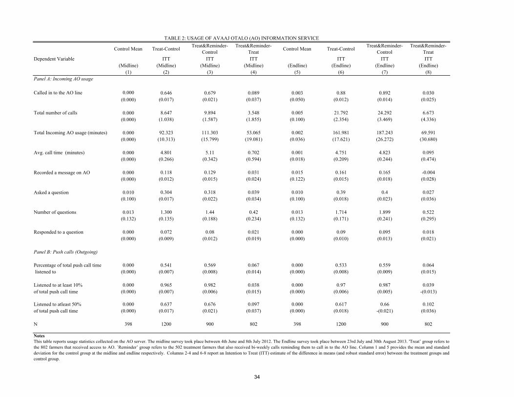
Control Mean Treat-Control Treat&Reminder-Control

Treat&Reminder-Treat Control Mean Treat-Control Treat&Reminder-

ControlTreat&Reminder-

TreatDependent Variable ITT ITT ITT ITT ITT ITT

(Midline) (Midline) (Midline) (Midline) (Endline) (Endline) (Endline) (Endline)(1) (2) (3) (4) (5) (6) (7) (8)

Panel A: Incoming AO usage

Called in to the AO line 0.000 0.646 0.679 0.089 0.003 0.88 0.892 0.030(0.000) (0.017) (0.021) (0.037) (0.050) (0.012) (0.014) (0.025)

Total number of calls 0.000 8.647 9.894 3.548 0.005 21.792 24.292 6.673(0.000) (1.038) (1.587) (1.855) (0.100) (2.354) (3.469) (4.336)

Total Incoming AO usage (minutes) 0.000 92.323 111.303 53.065 0.002 161.981 187.243 69.591(0.000) (10.313) (15.799) (19.081) (0.036) (17.621) (26.272) (30.680)

Avg. call time (minutes) 0.000 4.801 5.11 0.702 0.001 4.751 4.823 0.095(0.000) (0.266) (0.342) (0.594) (0.018) (0.209) (0.244) (0.474)

Recorded a message on AO 0.000 0.118 0.129 0.031 0.015 0.161 0.165 -0.004(0.000) (0.012) (0.015) (0.024) (0.122) (0.015) (0.018) (0.028)

Asked a question 0.010 0.304 0.318 0.039 0.010 0.39 0.4 0.027(0.100) (0.017) (0.022) (0.034) (0.100) (0.018) (0.023) (0.036)

Number of questions 0.013 1.300 1.44 0.42 0.013 1.714 1.899 0.522(0.132) (0.135) (0.188) (0.234) (0.132) (0.171) (0.241) (0.295)

Responded to a question 0.000 0.072 0.08 0.021 0.000 0.09 0.095 0.018(0.000) (0.009) (0.012) (0.019) (0.000) (0.010) (0.013) (0.021)

Panel B: Push calls (Outgoing)

Percentage of total push call time 0.000 0.541 0.569 0.067 0.000 0.533 0.559 0.064 listened to (0.000) (0.007) (0.008) (0.014) (0.000) (0.008) (0.009) (0.015)

Listened to at least 10% 0.000 0.965 0.982 0.038 0.000 0.97 0.987 0.039of total push call time (0.000) (0.007) (0.006) (0.015) (0.000) (0.006) (0.005) -(0.013)

Listened to atleast 50% 0.000 0.637 0.676 0.097 0.000 0.617 0.66 0.102of total push call time (0.000) (0.017) (0.021) (0.037) (0.000) (0.018) -(0.021) (0.036)

N 398 1200 900 802 398 1200 900 802

Notes

TABLE 2: USAGE OF AVAAJ OTALO (AO) INFORMATION SERVICE

This table reports usage statistics collected on the AO server. The midline survey took place between 4th June and 8th July 2012. The Endline survey took place between 23rd July and 30th August 2013. 'Treat’ group refers tothe 802 farmers that received access to AO. `Reminder’ group refers to the 502 treatment farmers that also received bi-weekly calls reminding them to call in to the AO line. Column 1 and 5 provides the mean and standarddeviation for the control group at the midline and endline respectively. Columns 2-4 and 6-8 report an Intention to Treat (ITT) estimate of the difference in means (and robust standard error) between the treatment groups andcontrol group.

34

Control Mean Treat vs. Control Treat vs. Control Treat&Reminder vs. Control

Treat&Reminder vs. Control

(Baseline) (Midline) (Endline) (Midline) (Endline)(1) (2) (3) (4) (5)

Panel A: Across all agricultural decisionsIndex of Mobile Phone-Based 0.000 1.829 1.259 1.848 1.236 Information Usage (standard deviation units) (0.289) (0.158) (0.099) (0.196) (0.116)

Used Mobile Phone-Based 0.093 0.616 0.704 0.621 0.698 Information (0.291) (0.031) (0.030) (0.032) (0.032)

Trust in Mobile Phone-Based 0.606 5.353 6.274 5.47 6.31 Information (on a scale of 1-10) (2.031) (0.262) (0.234) (0.277) (0.258)

Panel B: By decision typeCrop Decision 0.000 0.044 0.056 0.038 0.051

(0.000) (0.008) (0.010) (0.009) (0.011)

Pest Management 0.000 0.093 0.243 0.096 0.258(0.000) (0.011) (0.018) (0.014) (0.022)

Fertilizer Management 0.003 0.073 0.1 0.068 0.114(0.050) (0.011) (0.013) (0.013) (0.016)

Weather 0.003 0.234 0.369 0.242 0.362(0.050) (0.019) (0.022) (0.023) (0.026)

Soil Preparation 0.000 0.047 0.010 0.032 0.006(0.000) (0.008) (0.006) (0.008) (0.007)

Prices 0.023 -0.019 0.001 -0.014 0.010(0.149) (0.017) (0.016) (0.018) (0.018)

N 398 2323 2280 1743 1716

Notes

Difference-in-Difference Estimates (Treat*Post Coefficient)TABLE 3: EFFECTS ON SOURCES OF AGRICULTURAL INFORMATION

Dependent Variable

This table reports the impact of AO on usage of mobile phone-based information across different agricultural decisions. The indices aggregate information over multiple outcomes for which weexpect unidirectional treatment effects. Each index consists of the average of the z-scores for each component of the index, with the control group mean and standard deviation as reference. Mobilephone-based information usage index: Aggregates mobile phone use across crop decision, soil preparation, pest management, weather, cotton pesticides, cotton fertilizers, wheat fertilizers, cuminpesticides and cumin fertilizers. Data on agricultural decision-making and other information sources can be seen in Appendix Table A2. `Treat’ group refers to the 802 farmers that received access toAO. `Reminder’ group refers to the 502 treatment farmers that also received bi-weekly calls reminding them to call in to the AO line. The midline survey took place between 4th June and 8th July2012. The Endline survey took place between 23rd July and 30th August 2013. Column 1 provides the mean and standard deviation for the control group at baseline. Columns 2-5 report thecoefficient on the interaction term between a dummy for treatment and a dummy for the 'post' variable from a difference-in-difference specification. All specifications include village fixed effects, aswell as a control for the amount of baseline cotton grown and its interaction with the post variable.

35

Dependent Variable Control Mean Treat vs. Control Treat vs. Control Treat&Reminder vs. Control

Treat&Reminder vs. Control

(Baseline) (Midline) (Endline) (Midline) (Endline)(1) (2) (3) (4) (5)

Panel A: Expenditure on InputsTotal Input Expenditure 9.758 -0.020 0.099 -0.034 0.277(log rupees) (0.741) (0.162) (0.210) (0.179) (0.223)

Expenditure on Irrigation 4.821 1.009 0.605 1.118 0.817(log rupees) (4.469) (0.376) (0.369) (0.414) (0.404)

Panel B: Index of All Input-Related Decisions (standard deviation units)

Cotton 0.000 0.055 0.061 0.062 0.074(0.289) (0.028) (0.029) (0.034) (0.034)

Wheat 0.000 0.057 0.038 0.041 0.056(0.433) (0.036) (0.037) (0.038) (0.041)

Cumin 0.000 0.019 0.064 0.016 0.048(0.347) (0.036) (0.043) (0.040) (0.054)

Panel C: Index of Seed-Related Decisions (standard deviation units) Cotton 0.000 0.046 0.454 0.051 0.688

(0.296) (0.027) (0.280) (0.031) (0.432)

Wheat 0.000 -0.033 -0.032 -0.020 0.017(0.505) (0.070) (0.071) (0.066) (0.066)

Cumin 0.000 -0.020 0.012 -0.018 0.015(0.792) (0.072) (0.075) (0.084) (0.087)

Panel D: Indices of Pesticide-Related Decisions (standard deviation units) Cotton 0.000 0.028 0.062 0.038 0.081

(0.361) (0.036) (0.039) (0.040) (0.045)

Cumin 0.000 0.040 0.054 0.023 0.002(0.437) (0.043) (0.045) (0.047) (0.047)

Panel E: Indices of Fertilizer-Related Decisions (standard deviation units) Cotton 0.000 0.095 0.074 0.101 0.086

(0.457) (0.048) (0.044) (0.061) (0.052)

Wheat 0.000 0.043 0.028 0.046 0.036(0.553) (0.034) (0.046) (0.037) (0.051)

Cumin 0.001 -0.021 0.072 0.000 0.109(0.524) (0.051) (0.080) (0.054) (0.112)

N 398 2323 2280 1743 1716

Notes

TABLE 4: EFFECTS ON INPUT ADOPTION DECISIONS Difference-in-Difference Estimates (Treat*Post Coefficient)

This table reports the impact of AO on input decisions for seeds, pesticides and fertilizers. All coefficient estimates are in standard deviationunits. The indices aggregate information over multiple outcomes for which we expect unidirectional treatment effects. Each index consists ofthe average of the z-scores for each component of the index, with the control group mean and standard deviation as reference. Inputexpenditure includes total money spent on seeds, fertilizers, irrigation and pesticides for all crops in a year. All Input index: seed usage +pesticide purchase + pesticide usage + pesticide quantities + pesticide expenditure + fertilizer purchase + fertilizer usage + fertilizerquantities + fertilizer expenditure for the three different crops – cotton, wheat and cumin + irrigation expenditure. Pesticide managementindex: dummy to indicate purchase/use of a pesticide + pesticide expenditure + pesticide quantities across purchase and usage decisions.Fertilizer management index: dummy to indicate purchase/use of a fertilizer + fertilizer expenditure + fertilizer quantities across purchaseand usage decisions. Seed management index: dummy to indicate purchase/use of recommended seeds + seed expenditure + seed quantitiesacross purchase and usage decisions. `Treat’ group refers to the 802 farmers that received access to AO. `Reminder’ group refers to the 502treatment farmers that also received bi-weekly calls reminding them to call in to the AO line. The midline survey took place between 4thJune and 8th July 2012. The Endline survey took place between 23rd July and 30th August 2013. Column 1 provides the mean and standarddeviation for the control group at baseline. Columns 2-5 report the coefficient on the interaction term between a dummy for treatment and adummy for the 'post' variable from a difference-in-difference specification. All specifications include village fixed effects, as well as acontrol for the amount of baseline cotton grown and its interaction with the post variable.

36

Dependent Variable Control Mean Treat vs. Control Treat vs. Control Treat&Reminder vs. Control

Treat&Reminder vs. Control

(Baseline) (Midline) (Endline) (Midline) (Endline)(1) (2) (3) (4) (5)

Panel A: Sowing DecisionsPlanted Cotton 0.985 0.005 -0.002 0.001 0.001

(0.122) (0.011) (0.016) (0.012) (0.017)

Planted Wheat 0.776 0.047 0.069 0.023 0.061(0.417) (0.038) (0.039) (0.042) (0.042)

Planted Cumin 0.425 -0.015 -0.001 -0.007 0.004(0.495) (0.039) (0.040) (0.043) (0.044)

Panel B: Agricultural Outcomes (Expenditure, Profit, Yield)

Profit From Agriculture 11.463 0.056 0.075 0.051 0.093(log rupees) (0.989) (0.075) (0.091) (0.081) (0.099)

Cotton Yield 694.819 31.554 19.649 59.935 44.716(kg/acre) (468.752) (33.844) (33.480) (36.005) (35.466)

Wheat Yield 981.132 -33.693 -32.610 -49.903 -28.317(kg/acre) (702.002) (77.551) (71.201) (84.578) (76.883)

Cumin Yield 172.570 -7.169 48.295 0.074 54.27(kg/acre) (191.017) (23.731) (23.386) (26.822) (25.947)

N 398 2323 2280 1743 1716

Notes

TABLE 5: EFFECTS ON SOWING DECISIONS AND AGRICULTURAL PRODUCTIVITYDifference-in-Difference Estimates (Treat*Post Coefficient)

This table reports the impact of AO on sowing decisions and agricultural outcomes. Profit from agriculture refers to the difference between total incomefrom of all crops grown and total input expenditure (on seeds, pesticides, irrigation, fertilizers, hired labor and household labor priced at the mean wageof hired labor) in the past year. `Treat’ group refers to the 802 farmers that received access to AO. Column 1 provides the mean and standard deviationfor the control group at baseline.`Reminder’ group refers to the 502 treatment farmers that also received bi-weekly calls reminding them to call in to theAO line. The midline survey took place between 4th June and 8th July 2012. The Endline survey took place between 23rd July and 30th August 2013.Columns 2-5 report the coefficient on the interaction term between a dummy for treatment and a dummy for the 'post' variable from a difference-in-difference specification. All specifications include village fixed effects, as well as a control for the amount of baseline cotton grown and its interactionwith the post variable.

37

Dependent Variable Control Mean Treat vs. Control Treat vs. Control Treat&Reminder vs. Control

Treat&Reminder vs. Control

(Baseline) (Midline) (Endline) (Midline) (Endline)(1) (2) (3) (4) (5)

All Questions 14.156 0.492 0.760 0.525 0.619 (44 questions) (5.279) (0.438) (0.496) (0.480) (0.547)

Cotton-related 4.847 0.146 0.304 0.290 0.368 (20 questions) (1.989) (0.217) (0.234) (0.239) (0.257)

Wheat-related 3.419 0.108 0.063 0.081 -0.043 (7 questions) (1.629) (0.180) (0.149) (0.199) (0.164)

Cumin-related 5.164 0.098 -0.019 0.169 -0.078 (9 questions) (1.791) (0.241) (0.212) (0.263) (0.235)

Pesticide-related 0.887 0.018 0.048 0.074 0.064(8 questions) (0.717) (0.106) (0.107) (0.115) (0.117)

Fertilizer-related 0.606 0.055 0.072 0.042 0.081(3 questions) (0.656) (0.059) (0.065) (0.065) (0.072)

N 398 2323 2280 1743 1716

Notes

TABLE 6: EFFECT ON AGRICULTURAL KNOWLEDGEDifference-in-Difference Estimates (Treat*Post Coefficient)

This table reports the effect of AO on respondents’ agricultural knowledge. Respondents were asked agricultural questions across cropand topic, and a knowledge score was computed based on the proportion of correct answers. The question categories are not mutuallyexclusive. 'Treat’ group refers to the 802 farmers that received access to AO. 'Reminder’ group refers to the 502 treatment farmers thatalso received bi-weekly calls reminding them to call in to the AO line. The midline survey took place between 4th June and 8th July2012. The Endline survey took place between 23rd July and 30th August 2013. Column 1 provides the mean and standard deviation forthe control group baseline. Columns 2-5 report the coefficient on the interaction term between a dummy for treatment and a dummy forthe 'post' variable from a difference-in-difference specification. All specifications include village fixed effects, a control for the amountof baseline cotton grown and its interaction with the post variable.

38

Dependent Variable Control Mean Treat*Post*Educ Treat*Post*Educ Treat*Post*Inc Treat*Post*Inc(Midline) (Endline) (Midline) (Endline)

(1) (2) (3) (4) (5)Panel A: AO Usage

Called AO line 0.000 0.023 -0.021 0.051 -0.010(0.000) (0.038) (0.026) (0.035) (0.024)

Total Incoming 0.000 20.957 35.220 39.348 55.038 AO Usage (Minutes) (0.000) (22.909) (40.646) (18.930) (32.031)

Panel B: Indices of Input-related Practices (standard deviation units)

Cotton Management 0.000 -0.008 0.040 0.073 0.106(0.289) (0.054) (0.055) (0.053) (0.055)

Wheat Management 0.000 0.037 0.022 0.017 0.020(0.433) (0.061) (0.065) (0.068) (0.069)

Cumin Management 0.000 -0.048 -0.052 -0.059 0.057(0.347) (0.065) (0.089) (0.067) (0.081)

Pesticide Management 0.000 -0.028 -0.057 0.005 0.082(0.303) (0.059) (0.062) (0.058) (0.061)

Fertilizer Management 0.000 -0.012 0.054 0.028 0.093(0.306) (0.061) (0.091) (0.063) (0.078)

Panel C: Agricultural Knowledge Score

Total Correct Answers 14.156 0.210 1.256 -0.371 0.770 (44 questions) (5.279) (0.772) (0.913) (0.848) (0.982)

N 398 2323 2280 2323 2280

Notes

TABLE 7: HETEROGENEOUS EFFECTS BY EDUCATION AND INCOMETriple Difference Estimates

Education Income

This table tests for heterogeneity in the treatment effect across education and income level. Management practices indices: seed usage +pesticide purchase + pesticide usage + pesticide quantities + pesticide expenditure + fertilizer purchase + fertilizer usage + fertilizerquantities + fertilizer prices for the three different crops – cotton, wheat, and cumin. Pesticide management index: dummy to indicatepurchase/use of a pesticide + pesticide expenditure + pesticide quantities across purchase and usage decisions. Fertilizer managementindex: dummy to indicate purchase/use of a fertilizer + fertilizer expenditure + fertilizer quantities across purchase and usage decisions.Seed management index: dummy to indicate purchase/use of recommended seeds + seed expenditure + seed quantities across purchase andusage decisions. Education and income measures are all collected during the baseline survey, which took place in June 2011. Incomerefers to agricultural income for the past 12 months. ‘Treat’ group refers to the 802 farmers that received access to AO. The estimates arefrom the endline survey that took place between 23rd July and 30th August 2013. Column 1 provides the mean and standard deviation forthe control group at baseline. Columns 2 and 3 report the triple interactions from a triple difference specification with interactions withabove-median education, columns 4 and 5 report the same for above median income (the specifications also include the double interactionterms). Columns 2 and 4 are midline comparisons, while columns 3 and 5 are endline comparisons.

39

Control Mean Treat*Post

Fraction of Peers

Treated *Post

Fraction of Peers

Treated *Treat*Post

Treat*Post

Fraction of Peers

Treated *Post

Fraction of Peers

Treated *Treat*Post

Control Peer Group Mean

Fraction of Peers

Treated

Dependent Variable (Baseline)

(1) (2) (3) (4) (5) (6) (7) (8) (9)

Called AO line 0.000 0.538 -0.001 -0.036 0.65 0.001 -0.032 - -(0.000) (0.020) (0.012) (0.074) (0.019) (0.012) (0.071)

Total AO usage (Minutes) 0.000 54.981 -0.625 10.928 76.685 -1.217 15.689 - -(0.000) (4.752) (3.456) (17.499) (6.301) (4.422) (22.205)

Index of Mobile Phone-Based -0.000 1.947 0.047 -0.815 1.323 -0.154 -0.360 -0.000 -0.005 Information Usage (0.704) (0.171) (0.219) (0.597) (0.111) (0.132) (0.292) (0.878) (0.049)

Planted Cumin 0.425 -0.032 -0.031 0.108 -0.005 0.052 0.077 0.237 0.059(0.495) (0.045) (0.112) (0.146) (0.046) (0.116) (0.150) (0.425) (0.030)

Area of Cumin Planted 0.762 0.033 -0.097 0.151 -0.024 -0.023 0.413 0.525 0.255(Acres) (1.406) (0.120) (0.284) (0.376) (0.124) (0.307) (0.439) (1.695) (0.133)

Planted Wheat 0.776 0.014 -0.158 0.228 0.049 -0.100 0.114 0.253 -0.011(0.417) (0.044) (0.111) (0.145) (0.046) (0.117) (0.151) (0.435) (0.031)

Area of Wheat Planted 1.171 0.044 -0.026 -0.016 0.081 0.066 -0.090 0.328 -0.050(Acres) (1.346) (0.106) (0.231) (0.323) (0.104) (0.229) (0.322) (1.153) (0.077)

Proportion of Cotton Lost - - - - - - - 0.142 -0.039to Pest Attacks (%) (0.224) (0.015)

Cotton Pest Management 0.000 -0.005 -0.102 0.212 0.030 -0.155 0.185 0.000 0.087(0.361) (0.042) (0.084) (0.117) (0.047) (0.088) (0.114) (0.612) (0.054)

N 398 1846 1810 545 1114

TABLE 8: SPILLOVER AND PEER EFFECTSStudy Respondents Non-Study Respondents

NotesThis table assesses whether the fraction of one's peers assigned to the treatment group influences own outcomes and how this varies for study respondents and non-studyrespondents. The midline survey took place between 4th June and 8th July 2012. Columns 1-7 refer to study respondents, while columns 8-9 refer to non-study respondents.Columns 2-4 report coefficietns from a difference-in-difference specification using baseline and midline data, while columns 5-7 report the analogous coefficients using endlinedata. Column 1 reports the mean and standard deviation for the control group at baseline. Column 2 (5) resports the interaction between the treat variable and a dummy variablefor whether the observation is from the midline (endline). Column 3 (6) report the coefficient on the interaction of the number of peers who were assigned to the treatment group(Fraction of Peers Treated) and a dummy for whether the observation is from the midline (endline). Column 4 (7) resports the interaction between 'Fractions of Peers Treated' and'Treat*Post' defined for the midline (endline). Column 8 reports the mean and standard deviation for peers who were not respondents in the main study and who were notreferenced by a treatment respondent. Column 9 reports the coefficient on the number of peers who were assigned to the treatment group, from a regression of the characteristic inquestion on this variable. All regresson specification include dummies for the number of peers referenced, the amount of cotton grown at baseline, and village fixed effects.

(Midline) (Endline) (Peer Survey)

40

Cell Contents Participated in WTP (N) Bought AO (N) Avg. WTP for AO (rupees)(1) (2) (3)

Respondent Group:Entire Sample 1043 347 108.993

Study 586 209 121.246 Treatment 407 151 123.858 Control 179 58 115.307

Non-Study 457 138 93.282

Panel B: Predictors of Purchasing Avaaj Otalo (AO)Dependent Variable Bought AO Bought AO Bought AO Bought AO Bought AO Bought AO Bought AO Bought AO

(1) (2) (3) (4) (5) (6) (7) (8)

Offer Price -0.001 -0.001 -0.001 -0.001 -0.001 -0.001 -0.001 -0.001(0.000) (0.000) (0.000) (0.000) (0.000) (0.000) (0.000) (0.000)

Treatment Status -0.019 -0.02 -0.02 -0.019 -0.019 -0.019 -0.019 -0.02(0.010) (0.010) (0.010) (0.010) (0.011) (0.010) (0.010) (0.010)

Years of Education 0.009 0.008(0.002) (0.002)

Total Correct Answers to 0.003 0.001 Knowledge Questions (0.002) (0.002)

Total Area of Cotton Planted (Acres) 0.001 0.001(0.002) (0.002)

Referrals in the Treatment Group -0.001 -0.001(0.020) (0.020)

Skepticism toward Technology -0.018 -0.013(0.020) (0.020)

Age of Household Head -0.001 -0.001(0.001) (0.001)

N 7885 7885 7885 7885 7885 7885 7885 7885N(Clusters) 1200 1200 1200 1200 1200 1200 1200 1200

Notes

TABLE 9: RESULTS FROM WILLINGNESS TO PAY EXPERIMENTSPanel A: Average Willingness to Pay in BDM Exercise

This table reports results from the willingness to pay study that was carried out between 23rd July and 30th August 2013 along with the endline paper survey. Respondents took part in two types of willingness to pay exercises – 75%participated in bidding game based on the Becker-Degroot-Marschak (BDM) method and 25% participated in a simpler take-it-or-leave-it (TIOLI) exercise. Panel A reports the mean maximum willingness to pay for the AO service by treatmentstatus for all those respondents that participated in the BDM exercise. Column 1 refers to the number of respondents from each respondent group that participated in the BDM experiment. Column 2 refers to the fraction of respondents thatpurchased AO from those that participated in the exercise. Column 3 refers to the average willingness to pay for AO (in rupees) by respondent group. Study: Treatment + Control. Entire Sample: Study + Non-Study. Panel B reports predictorsof willingness to pay for the service based on characteristics from the baseline survey and the bids placed during the willingness to pay exercise. This table includes only those farmers that were part of the treatment or control group. Skepticismtowards technology is measured by a dummy that codes the question 'I am skeptical of new technologies'. Referrals in the treatment group refer to those respondents who referenced peers - a maximum of three were elicited - who werethemselves assigned to treatment.

41

Cell Contents Midline Endline Midline Endline Midline Endline Midline Endline(1) (2) (3) (4) (5) (6) (7) (8)

Panel A: By CropCotton 679 960 0.50 0.46 30 59 0.68 0.62

Cumin 80 151 0.06 0.07 15 36 0.34 0.38

Wheat 26 43 0.02 0.02 11 27 0.25 0.28

Panel B: By ThemePest Management 739 1126 0.54 0.54 23 73 0.52 0.77

Crop Planning 197 363 0.14 0.17 30 64 0.68 0.67

Fertilizer 106 154 0.08 0.07 13 32 0.30 0.34

Weather 66 88 0.05 0.04 10 26 0.23 0.27

Irrigation 12 21 0.01 0.01 2 5 0.05 0.05

N 1370 2079 44 95

NotesThis table reports information on push calls and questions asked on the AO server, categorized by crop and theme. All push calls containinformation on multiple themes. A total of 95 push calls were sent out during September 2011- August 2013, with an average length ofapproximately 5 minutes. The midline survey took place between 4th June and 8th July 2012. The Endline survey took place between 23rdJuly and 30th August 2013.

APPENDIX TABLE A1: TOPICS OF QUESTION ASKED AND PUSH CALLS No. of Questions % of Total Questions No. of Push Calls % of Total Push Calls

42

Dependent Variable Control AOE AOE-C AO AO-CMean Mean ITT Mean ITT

(1) (2) (3) (4) (5)Panel A: Sample SizeEntire Sample 398 403 801 399 797

Panel B: Individual CharacteristicsAge 46.539 45.692 -0.832 46.610 0.098

(15.161) (14.687) (1.049) (14.995) (1.061)

Years of Education 4.235 4.089 -0.118 3.967 -0.252(3.836) (3.897) (0.263) (3.970) (0.272)

Landholdings- Acres 6.077 6.332 0.232 6.017 -0.044(5.596) (5.874) (0.385) (6.179) (0.396)

Agricultural Income 11.551 11.528 -0.022 11.558 0.011(log rupees) (1.361) (1.470) (0.098) (1.465) (0.099)

Panel C: Indices (standard deviation units) Mobile Phone-based 0.000 -0.001 0.000 0.050 0.050 Information Usage (0.704) (0.702) (0.050) (0.995) (0.061)

Cotton Management 0.000 -0.005 -0.004 0.007 0.007(0.289) (0.281) (0.020) (0.335) (0.022)

Wheat Management 0.000 -0.043 -0.042 -0.005 -0.006(0.433) (0.329) (0.027) (0.449) (0.030)

Cumin Management 0.000 0.007 0.011 -0.019 -0.019(0.347) (0.577) (0.032) (0.317) (0.022)

Pesticide Management 0.000 -0.012 -0.011 -0.002 -0.002(0.303) (0.309) (0.021) (0.324) (0.021)

Fertilizer Management 0.000 0.006 0.009 -0.014 -0.015(0.306) (0.500) (0.028) (0.354) (0.022)

Seed Management 0.000 -0.002 -0.002 0.038 0.037(0.244) (0.440) (0.025) (0.359) (0.021)

Panel D: Historical Agricultural ActivityPlanted Cotton (2010) 0.985 0.988 0.002 0.977 -0.008

(0.122) (0.111) (0.008) (0.149) (0.009)

Area Cotton Planted - Acres (2010) 4.448 4.736 0.277 5.014 0.573(3.622) (4.426) (0.281) (4.045) (0.269)

Planted Cotton (2011) 0.984 0.984 0.000 0.986 0.003-0.126 (0.125) (0.009) (0.116) (0.009)

Area Cotton Planted - Acres (2011) 4.990 5.417 0.382 5.204 0.221(3.846) (4.852) (0.308) (4.006) (0.281)

Planted Wheat (2010) 0.776 0.722 -0.053 0.724 -0.053(0.417) (0.449) (0.029) (0.447) (0.029)

Area Wheat Planted- Acres (2010) 1.171 1.067 -0.100 1.314 0.135(1.346) (1.248) (0.088) (2.180) (0.123)

Planted Cumin (2010) 0.425 0.412 -0.014 0.401 -0.023(0.495) (0.493) (0.033) (0.491) (0.032)

Area Cumin Planted - Acres (2010) 0.762 0.705 -0.057 0.789 0.018(1.406) (1.343) (0.095) (1.499) (0.097)

Notes

APPENDIX TABLE A2: SUMMARY STATISTICS AND BALANCE BY TREATMENT GROUP (AO AND AOE)

This table reports summary statistics and balance by treatment group using data from the baseline survey, conducted between June 26 and August 11,2011. Participants were randomized into three groups. AO group received AO access. AOE group received AO access and physical extension. Thecontrol group received neither treatment. The indices aggregate information over multiple outcomes for which we expect unidirectional treatmenteffects. Each index consists of the average of the z-scores for each component of the index, with the control group mean and standard deviation asreference. Mobile phone-based information usage index: Aggregates mobile phone use across crop decision, soil preparation, pest identification,weather, cotton pesticides, cotton fertilizers, wheat fertilizers, cumin pesticides and cumin fertilizers. Management practices indices: seed usage +pesticide purchase + pesticide usage + pesticide quantities + pesticide expenditure + fertilizer purchase + fertilizer usage + fertilizer quantities +fertilizer expenditure for the three different crops – cotton, wheat and cumin. Pesticide management index: dummy to indicate purchase/use of apesticide + pesticide expenditure + pesticide quantities across purchase and usage decisions. Fertilizer management index: dummy to indicatepurchase/use of a fertilizer + fertilizer expenditure + fertilizer quantities across purchase and usage decisions. Seed management index: dummy toindicate purchase/use of recommended seeds + seed expenditure + seed quantities across purchase and usage decisions. Agricultural income refers toincome earned from all crops over the past 12 months. Column 1, 2 and 4 show the summary statistics (mean and standard deviation) for the controlgroup at baseline. Columns 3 and 5 report an Intention to Treat (ITT) estimate of the difference in means (and robust standard error) between thetreatment groups (AO and AOE) and the control group.

43

APPENDIX TABLE A3: MAIN EFFECTS BY TREATMENT GROUP (AO and AOE)

Cells Contents: Control Mean AOE vs. Control AOE vs. Control AO vs. Control AO vs. Control

(Baseline) (Midline) (Endline) (Midline) (Endline)(1) (2) (3) (4) (5)

Panel A: AO UsageCalled in to the AO line 0.000 0.548 0.65 0.506 0.611

(0.000) (0.025) (0.024) (0.025) (0.025)

Total duration of calling in time 0.000 97.421 125.564 61.091 83.249 (Minutes) (0.000) (16.113) (20.851) (8.398) (10.407)

Panel B: Indices (standard deviation units) Mobile Phone-Based -0.000 2.24 1.38 1.394 1.127 Information Usage (0.704) (0.231) (0.133) (0.195) (0.128)

Cotton Management 0.000 0.069 0.075 0.042 0.049(0.289) (0.037) (0.034) (0.031) (0.035)

Wheat Management -0.000 0.063 0.050 0.053 0.027(0.433) (0.039) (0.041) (0.043) (0.043)

Cumin Management 0.000 -0.016 0.012 0.047 0.11(0.347) (0.045) (0.045) (0.044) (0.062)

Pesticide Management 0.000 0.020 0.056 0.048 0.059(0.303) (0.035) (0.037) (0.041) (0.040)

Fertilizer Management 0.000 0.047 0.033 0.048 0.100(0.306) (0.045) (0.037) (0.036) (0.067)

Panel C: Sowing DecisionsPlanted Cotton 0.985 -0.002 -0.002 0.012 -0.002

(0.122) (0.012) (0.017) (0.013) (0.019)

Planted Wheat 0.776 0.044 0.08 0.047 0.056(0.417) (0.044) (0.045) (0.045) (0.045)

Planted Cumin 0.425 -0.031 -0.000 -0.003 -0.003(0.495) (0.045) (0.046) (0.045) (0.046)

Panel D: Agricultural Outcomes (Input Expenditure, Profit, Yield) Total Input Expenditure 9.758 0.163 0.179 -0.199 0.025(log rupees) (0.741) (0.180) (0.240) (0.200) (0.242)

Total profit 11.463 0.059 0.029 0.119 0.089(log rupees) (0.989) (0.092) (0.149) (0.091) (0.135)

Cotton Yield 694.819 14.968 4.358 49.256 35.137(kg/acre) (468.752) (39.144) (39.568) (37.905) (36.641)

Wheat Yield 981.132 -90.107 1.048 25.363 -81.650(kg/acre) (702.002) (88.367) (85.476) (95.205) (79.429)

Cumin Yield 172.570 -20.500 29.530 5.614 70.126(kg/acre) (191.017) (29.383) (27.173) (24.958) (26.755)

Panel E: Agricultural KnowledgeTotal Correct Answers 14.156 0.315 0.523 0.661 1 (44 questions) (5.279) (0.494) (0.568) (0.517) (0.583)

N 398 1557 1525 1539 1512

Notes

Difference-in-Difference Estimates (Treat*Post Coefficient)

This table reports the main treatment effects for the two treatment groups – AOE and AO. The AOE group refers to the 403 treatmentrespondents that had access to AO along with physical extension. AO group refers to the 399 treatment respondents that only had access to AO.The midline survey took place between 4th June and 8th July 2012. The Endline survey took place between 23rd July and 30th August 2013. Theindices aggregate information over multiple outcomes for which we expect unidirectional treatment effects. Each index consists of the average ofthe z-scores for each component of the index, with the control group mean and standard deviation as reference. Mobile phone-based informationusage index: Aggregates mobile phone use across crop decision, soil preparation, pest identification, weather, cotton pesticides, cotton fertilizers,wheat fertilizers, cumin pesticides and cumin fertilizers. Management practices indices: seed usage + pesticide purchase + pesticide usage +pesticide quantities + pesticide expenditure + fertilizer purchase + fertilizer usage + fertilizer quantities + fertilizer expenditure for the threedifferent crops – cotton, wheat and cumin. Pesticide management index: dummy to indicate purchase/use of a pesticide + pesticide expenditure+ pesticide quantities across purchase and usage decisions. Fertilizer management index: dummy to indicate purchase/use of a fertilizer +fertilizer expenditure + fertilizer quantities across purchase and usage decisions. Seed management index: dummy to indicate purchase/use ofrecommended seeds + seed expenditure + seed quantities across purchase and usage decisions. Total input expenditure refers to money spent onseeds, fertilizers, pesticides and irrigation in the past year. Profit from agriculture is the difference between revenue from all crops and total inputexpenditure in the past year. Respondents were asked agricultural questions across crop and topic, and a knowledge score was computed basedon the proportion of correct answers. Column 1 provides the mean and standard deviation for the control group at baseline. Columns 2-5 reportthe coefficient on the interaction term between a dummy for treatment and a dummy for the 'post' variable from a difference-in-differencespecification. All specifications include village fixed effects, as well as a control for the amount of baseline cotton grown and its interaction withthe post variable.

44

1% 5% 10% 1% 5% 10%(1) (2) (3) (4) (5) (6)

Panel A. Baseline

Variables with Imbalance 17 101 217 20 84 193Total Number of Variables in Baseline 2295 2295 2295 2295 2295 2295Imbalance Percentage in Baseline 0.007 0.044 0.095 0.009 0.037 0.084

Panel B. Midline

Variables with Imbalance 189 317 457 161 256 366Total Number of Variables in Midline 2704 2704 2704 2704 2704 2704Imbalance Percentage in Midline 0.070 0.117 0.169 0.060 0.095 0.135

Panel C. Endline

Variables with Imbalance 178 307 465 151 269 414Total Number of Variables in Endline 2587 2587 2587 2587 2587 2587Imbalance Percentage in Endline 0.069 0.119 0.180 0.058 0.104 0.160

Notes:

APPDENDIX A4: RANDOMIZATION CHECK

Treat vs Control Treat&Reminder vs. ControlNo. of Variables Significantly Different from Control at Following Levels of Statistical Significance

This tables reports balance tests between the combined treatment group (AO+AOE) and the control group (columns 1-3) and the treatment group receiving reminder calls and the controlgroup (columns 4-6) for all variables at baseline (Panel A), midline survey (Panel B) and endline survey (Panel C). Variables with Imbalance' refers to the number of variables where thetreatment group mean is significantly different from the control group mean at traditional levels of statistical significance. Columns 1 and 4 report the corresponding number at the 1%level, columns 2 and 5 at the 5% level and columns 3 and 6 at the 10% level. The 'Imbalance Percentage' refers to the number of variables where there is an imbalance between treatmentand control over the total number of variables collected. 'Imbalance Percentage suggested by Chance' is the fraction of variables where we would expect a difference between treatment andcontrol as a consequence of the distribution of the test-statistic (t-distribution) and Type 1 error.

45

Impact of AO on Information Sources UsedSource of Information

Control Treat-Control Treat-Control Control Treat-Control Treat-Control Control Treat-Control Treat-Control Control Treat-Control Treat-Control Control Treat-Control Treat-ControlDependent Variable Mean ITT ITT Mean ITT ITT Mean ITT ITT Mean ITT ITT Mean ITT ITT

(Baseline) (Midline) (Endline) (Baseline) (Midline) (Endline) (Baseline) (Midline) (Endline) (Baseline) (Midline) (Endline) (Baseline) (Midline) (Endline)(1) (2) (3) (4) (5) (6) (7) (8) (9) (10) (11) (12) (10) (11) (12)

Decision TypeCotton Planting 0.020 0.008 0.008 0.000 0.074 0.086 0.296 0.017 0.034 0.080 -0.017 -0.010 0.005 0.004 0.004

(0.141) (0.015) (0.012) (0.000) (0.010) (0.011) (0.457) (0.039) (0.038) (0.272) (0.023) (0.023) (0.071) (0.004) (0.004)

Cotton Fertilizers 0.020 0.011 0.003 0.003 0.062 0.071 0.227 -0.001 0.035 0.099 0.015 0.05 0.003 0.000 0.003(0.142) (0.010) (0.012) (0.051) (0.009) (0.010) (0.419) (0.032) (0.032) (0.300) (0.021) (0.022) (0.051) (0.004) (0.003)

Cotton Pesticides 0.023 -0.001 0.011 0.000 0.152 0.162 0.399 -0.031 0.007 0.440 -0.072 -0.037 0.003 -0.004 -0.004(0.149) (0.013) (0.012) (0.000) (0.013) (0.014) (0.490) (0.039) (0.037) (0.497) (0.041) (0.037) (0.050) (0.004) (0.004)

Wheat Planting 0.008 -0.002 0.003 0.000 0.112 0.022 0.116 -0.016 0.004 0.023 -0.003 0.005 0.000 -0.005 0.000(0.087) (0.008) (0.007) (0.000) (0.012) (0.007) (0.320) (0.023) (0.023) (0.149) (0.011) (0.011) (0.000) (0.004) (0.000)

Wheat Fertilizers 0.005 -0.003 0.003 0.000 0.014 0.009 0.111 0.009 0.004 0.055 0.014 0.020 0.000 0.000 0.000(0.071) (0.006) (0.006) (0.000) (0.004) (0.004) (0.314) (0.021) (0.021) (0.229) (0.015) (0.014) (0.000) (0.000) (0.000)

Wheat Pesticides 0.005 0.001 0.004 0.000 0.012 0.003 0.023 0.004 -0.006 0.013 0.004 0.003 0.000 0.000 0.000(0.071) (0.004) (0.005) (0.000) (0.004) (0.004) (0.149) (0.011) (0.010) (0.112) (0.010) (0.008) (0.000) (0.000) (0.000)

Cumin Planting 0.003 -0.002 -0.005 0.000 0.153 0.049 0.093 -0.019 -0.027 0.065 0.019 0.037 0.003 -0.003 0.003(0.050) (0.008) (0.007) (0.000) (0.013) (0.009) (0.291) (0.024) (0.023) (0.247) (0.018) (0.017) (0.050) (0.004) (0.003)

Cumin Fertilizers 0.000 -0.008 -0.001 0.000 0.015 0.016 0.068 -0.005 0.020 0.025 -0.010 -0.000 0.000 0.000 0.000(0.000) (0.004) (0.002) (0.000) (0.004) (0.006) (0.252) (0.018) (0.017) (0.157) (0.011) (0.011) (0.000) (0.000) (0.000)

Cumin Pesticides 0.005 0.000 0.002 0.000 0.029 0.043 0.126 0.001 0.018 0.133 -0.026 -0.003 0.000 0.000 0.000(0.071) (0.006) (0.005) (0.000) (0.006) (0.009) (0.332) (0.024) (0.023) (0.340) (0.027) (0.024) (0.000) (0.000) (0.000)

N 398 2323 2280 398 2323 2280 398 2323 2280 398 2323 2280 398 2323 2280

Notes

Government Extension Workers

This table reports the impact of AO on usage of different information sources for agricultural decision-making over time. First, we asked survey participants if they received information for a particular decision making category. Then, participants were asked toname their most important source for this category. ‘Treat’ group refers to the 802 farmers that received access to AO. The midline survey took place between 4th June and 8th July 2012. The Endline survey took place between 23rd July and 30th August 2013.Column 1, 4, 7 and 10 provides the mean and standard deviation for the control group by information source at baseline. Columns 2-3, 5-6, 8-9 and 11-12 report the Intention to Treat (ITT) estimate of the difference in means (and robust standard error) between thetreatment groups and control group by information source.

APPENDIX TABLE A5: EFFECTS ON SOURCES OF INFORMATION BY SOURCE AND DECISION TYPE

Past Experience Mobile Phone-Based Information Other Farmers Input Dealers

46

APPENDIX TABLE A6: BREAKDOWN OF INPUT COSTS

Dependent Variable Control Mean Treat vs. Control Treat vs. Control Treat&Reminder vs. Control

Treat&Reminder vs. Control

(Baseline) (Midline) (Endline) (Midline) (Endline)(1) (2) (3) (4) (5)

Panel A: AcreageTotal Acres of Cotton 4.448 -0.031 0.115 -0.071 0.250

(3.622) (0.181) (0.182) (0.198) (0.209)

Total Acres of Wheat 1.171 0.050 0.086 0.022 0.079(1.346) (0.092) (0.089) (0.109) (0.106)

Total Acres of Cumin 0.762 0.055 0.005 0.060 0.012(1.406) (0.109) (0.113) (0.122) (0.126)

Panel B: Input CostsTotal input expenditure 9.758 -0.020 0.099 -0.034 0.277(log rupees) (0.741) (0.162) (0.210) (0.179) (0.223)

Expenditure on seeds 6.105 0.071 0.309 0.023 0.416(log rupees) (3.359) (0.281) (0.271) (0.311) (0.298)

Expenditure on fertilizers 8.914 0.085 -0.017 0.091 0.014(log rupees) (0.898) (0.102) (0.145) (0.110) (0.156)

Expenditure on pesticides 6.587 -0.212 -0.089 -0.255 -0.022(log rupees) (2.725) (0.213) (0.240) (0.234) (0.258)

Expenditure on irrigation 4.821 1.009 0.605 1.118 0.817(log rupees) (4.469) (0.376) (0.369) (0.414) (0.404)

Expenditure on hired labor 1.141 -0.140 -0.191 -0.259 -0.205(log rupees) (2.492) (0.204) (0.182) (0.221) (0.199)

Expenditure on household labor 6.594 -0.055 -0.011 -0.096 0.078(log rupees) (1.150) (0.134) (0.153) (0.148) (0.165)

N 398 2323 2280 1743 1716

Notes

Difference-in-Difference Estimates (Treat*Post Coefficient)

This table reports a detailed break-down of the input costs, aggregated across cotton, cumin and wheat. All expenditure figures are computed on a yearly basis.Total input expenditure refers to money spent on pesticides, fertilizers, seeds and irrigation. `Treat’ group refers to the 802 farmers that received access to AO.`Reminder’ group refers to the 502 treatment farmers that also received bi-weekly calls reminding them to call in to the AO line. The midline survey took placebetween 4th June and 8th July 2012. The Endline survey took place between 23rd July and 30th August 2013. Column 1 provides the mean and standarddeviation for the control group at baseline. Columns 2-5 report the coefficient on the interaction term between a dummy for treatment and a dummy for the 'post'variable from a difference-in-difference specification. All specifications include village fixed effects, as well as a control for the amount of baseline cotton grownand its interaction with the post variable.

47

Dependent Variable Control Mean Treat vs. Control Treat vs. Control Treat&Reminder vs. Control

Treat&Reminder vs. Control

(Baseline) (Midline) (Endline) (Midline) (Endline)(1) (2) (3) (4) (5)

Panel A: PesticidesIndex for pesticide management 0.000 0.031 0.057 0.028 0.041 practices (0.303) (0.030) (0.032) (0.033) (0.035)

Purchased monocrotophos 0.854 0.001 -0.025 -0.010 -0.018(0.353) (0.024) (0.028) (0.026) (0.030)

Quantity of monocrotophos purchased 2.878 0.087 0.086 0.071 0.084(liter) (3.756) (0.276) (0.230) (0.307) (0.260)

Total spent on monocrotophos 2.856 -0.348 -0.258 -0.456 -0.262(log rupees) (3.323) (0.250) (0.264) (0.278) (0.289)

Used monocrotophos 0.721 -0.011 -0.030 -0.010 -0.018(0.449) (0.029) (0.033) (0.032) (0.036)

Quantity of monocrotophos used 2.259 0.061 0.058 0.218 0.202(liter) (3.383) (0.281) (0.239) (0.313) (0.268)

Purchased imidachloropid 0.480 0.029 0.031 0.037 0.038(0.500) (0.042) (0.042) (0.046) (0.046)

Quantity of imidachloropid purchased 0.498 0.043 0.034 0.098 0.058(liter) (0.972) (0.095) (0.075) (0.110) (0.084)

Total spent on imidachloropid 2.588 -0.032 0.078 0.094 0.228(log rupees) (3.370) (0.297) (0.275) (0.327) (0.302)

Used imidachloropid 0.440 0.021 0.022 0.027 0.025(0.497) (0.042) (0.042) (0.046) (0.046)

Quantity of imidachloropid used 0.208 0.054 0.056 0.131 0.110(liter) (0.865) (0.092) (0.073) (0.100) (0.075)

Purchased acephate 0.899 0.016 -0.020 -0.002 -0.013(0.301) (0.025) (0.028) (0.028) (0.031)

Quantity of acephate purchased 2.536 0.182 0.057 0.074 0.003(kgs) (2.838) (0.240) (0.195) (0.264) (0.222)

Total spent on acephate 5.576 -0.279 -0.113 -0.337 -0.025(log rupees) (2.889) (0.243) (0.252) (0.270) (0.275)

Used acephate 0.882 0.033 -0.001 0.016 0.000(0.323) (0.026) (0.030) (0.029) (0.033)

Quantity of acephate used 1.109 -0.093 0.014 -0.146 0.007(kgs) (2.966) (0.317) (0.221) (0.349) (0.258)

Purchased acetamaprid 0.274 0.050 0.027 0.029 0.014(0.447) (0.040) (0.040) (0.044) (0.045)

Quantity of acetamaprid purchased 0.163 -0.014 0.047 -0.018 -0.009(liter) (0.470) (0.060) (0.056) (0.068) (0.052)

Total spent on acetamaprid 1.432 0.218 0.205 0.141 0.126(log rupees) (2.670) (0.255) (0.242) (0.280) (0.268)

Used acetamaprid 0.216 0.021 -0.002 0.010 -0.012(0.412) (0.039) (0.039) (0.043) (0.044)

Quantity of acetamaprid used 0.077 -0.066 0.038 -0.061 0.036(liter) (0.572) (0.075) (0.054) (0.082) (0.063)

Biological method of pest controlUsed tricoderma 0.025 0.021 0.024 0.021 0.021

(0.157) (0.008) (0.009) (0.009) (0.009)

N 398 2323 2280 1743 1716

Notes

APPENDIX TABLE A7: BREAKDOWN OF INPUT ADOPTION DECISIONS Difference-in-Difference Estimates (Treat*Post Coefficient)

This table reports a detailed break-down of the impact of AO on purchase and usage decisions for agricultural inputs, aggregated across cotton, cumin and wheat. The indices aggregate information over multiple outcomes for which we expect unidirectional treatment effects. Each index consists of the average of the z-scores for each component of the index, with the control group mean and standard deviation as reference. Pesticide management index: dummy to indicate purchase/use of a pesticide + pesticide expenditure + pesticide quantities across purchase and usage decisions. Fertilizer management index: dummy to indicate purchase/use of a fertilizer + fertilizer expenditure + fertilizer quantities across purchase and usage decisions. Seed management index: dummy to indicate purchase/use of recommended seeds + seed expenditure + seed quantities across purchase and usage decisions. `Treat’ group refers to the 802 farmers that received access to AO. `Reminder’ group refers to the 502 treatment farmers that also received bi-weekly calls reminding them to call in to the AO line. The midline survey took place between 4th June and 8th July 2012. The Endline survey took place between 23rd July and 30th August 2013. Column 1 provides the mean and standard deviation for the control group at baseline. Columns 2-5 report the coefficient on the interaction term between a dummy for treatment and a dummy for the 'post' variable from a difference-in-difference specification. All specifications include village fixed effects, as well as a control for the amount of baseline cotton grown and its interaction with the post variable.

48

Dependent Variable Control Mean Treat vs. Control Treat vs. Control Treat&Reminder vs. Control

Treat&Reminder vs. Control

(Baseline) (Midline) (Endline) (Midline) (Endline)(1) (2) (3) (4) (5)

Panel B: FertilizersIndex of fertilizer management 0.000 0.068 0.069 0.078 0.090 practices (0.306) (0.043) (0.042) (0.050) (0.059)

Purchased urea 0.987 -0.004 -0.012 -0.005 -0.005(0.112) (0.012) (0.018) (0.013) (0.020)

Quantity of urea purchased 653.804 -62.619 -56.620 21.827 32.707(kgs) (561.062) (74.123) (72.128) (37.359) (36.975)

Total spent on urea 7.851 0.105 -0.018 0.068 0.026(log rupees) (1.301) (0.119) (0.159) (0.130) (0.170)

Used urea 0.987 -0.005 -0.014 -0.007 -0.007(0.112) (0.012) (0.018) (0.013) (0.020)

Quantity of urea used 627.839 -10.507 4.150 -41.591 8.856(kgs) (502.653) (55.515) (35.132) (53.111) (40.634)

Purchased di-ammonium phosphate 0.975 -0.016 -0.022 -0.021 -0.021(0.157) (0.015) (0.021) (0.016) (0.022)

Quantity of di-ammonium phosphate 614.899 -12.895 -11.553 126.326 138.777purchased (kgs) (2122.793) (137.179) (137.215) (111.143) (111.055)

Total spent on di-ammonium phosphate 8.069 0.003 -0.180 -0.061 -0.171(log rupees) (1.677) (0.156) (0.195) (0.166) (0.207)

Used di-ammonium phosphate 0.975 -0.014 -0.016 -0.021 -0.018(0.157) (0.016) (0.021) (0.017) (0.022)

Quantity of di-ammonium phosphate used 505.075 49.022 17.532 80.190 25.138(kgs) (555.683) (81.177) (33.977) (113.569) (38.892)

Purchased ammonium sulphate 0.078 0.057 0.045 0.047 0.039(0.268) (0.024) (0.021) (0.026) (0.024)

Quantity of ammonium sulphate purchased 7.839 7.620 3.221 6.042 2.586(kgs) (48.033) (4.774) (4.297) (5.150) (4.625)

Total spent on ammonium sulphate 0.514 0.368 0.322 0.299 0.275(log rupees) (1.812) (0.162) (0.144) (0.179) (0.159)

Used ammonium sulphate 0.078 0.056 0.045 0.047 0.036(0.268) (0.024) (0.021) (0.026) (0.023)

Quantity of ammonium sulphate used 11.332 11.3 5.722 8.164 5.179(kgs) (58.119) (5.474) (4.544) (5.488) (4.864)

Purchased NPK grade 1 (for Cotton only) 0.113 0.026 0.055 0.042 0.0740.317 (0.033) (0.030) (0.036) (0.033)

Quantity of NPK grade 1 purchased (for Cotton only) 1.357 5.188 10.622 5.092 14.137(kgs) 14.655 (7.704) (7.556) (8.875) (9.072)

Total spent on NPK grade 1 (for Cotton only) 0.797 -0.074 0.377 0.044 0.519(log rupees) 2.276 (0.147) (0.225) (0.158) (0.248)

Used NPK grade 1 (for Cotton only) 0.113 0.029 0.053 0.043 0.070.317 (0.033) (0.030) (0.036) (0.033)

Quantity of NPK grade 1 used (for Cotton only) 1.484 4.993 10.757 4.481 14.119(kgs) 14.704 (7.591) (7.343) (8.715) (8.899)

Organic/Bio-FertilizersUsed manure 0.168 0.041 0.036 0.064 0.054

(0.375) (0.031) (0.028) (0.034) (0.030)

Purchased bio-fertilizers 0.005 0.001 0.001 0.003 -0.002(0.071) (0.006) (0.006) (0.007) (0.006)

N 398 2323 2280 1743 1716

Notes

APPENDIX TABLE A7: BREAKDOWN OF INPUT ADOPTION DECISIONS (CONTD…)Difference-in-Difference Estimates (Treat*Post Coefficient)

This table reports a detailed break-down of the impact of AO on purchase and usage decisions for agricultural inputs, aggregated across cotton, cumin and wheat. The indices aggregate information over multiple outcomes for which we expect unidirectional treatment effects. Each index consists of the average of the z-scores for each component of the index, with the control group mean and standard deviation as reference. Pesticide management index: dummy to indicate purchase/use of a pesticide + pesticide expenditure + pesticide quantities across purchase and usage decisions. Fertilizer management index: dummy to indicate purchase/use of a fertilizer + fertilizer expenditure + fertilizer quantities across purchase and usage decisions. Seed management index: dummy to indicate purchase/use of recommended seeds + seed expenditure + seed quantities across purchase and usage decisions. `Treat’ group refers to the 802 farmers that received access to AO. `Reminder’ group refers to the 502 treatment farmers that also received bi-weekly calls reminding them to call in to the AO line. The midline survey took place between 4th June and 8th July 2012. The Endline survey took place between 23rd July and 30th August 2013. Column 1 provides the mean and standard deviation for the control group at baseline. Columns 2-5 report the coefficient on the interaction term between a dummy for treatment and a dummy for the 'post' variable from a difference-in-difference specification. All specifications include village fixed effects, a control for the amount of baseline cotton grown and its interaction with the post variable.

49

Dependent Variable Control Mean Treat vs. Control Treat vs. Control Treat&Reminder vs. Control

Treat&Reminder vs. Control

(Baseline) (Midline) (Endline) (Midline) (Endline)(1) (2) (3) (4) (5)

Panel C: SeedsIndex of seed management practices -0.000 0.023 0.295 0.029 0.460

(0.244) (0.025) (0.185) (0.027) (0.286)

Solicited advice for seeds 0.666 -0.006 0.029 0.004 0.035(0.472) (0.042) (0.042) (0.046) (0.046)

Purchased recommended seeds 0.844 0.030 0.048 0.024 0.065(0.363) (0.033) (0.032) (0.036) (0.036)

Used recommended seeds 0.869 0.036 0.053 0.032 0.07(0.337) (0.031) (0.031) (0.034) (0.034)

Quantity of recommended seeds purchased 50.873 22.895 41.378 15.142 46.513(kgs) (388.567) (20.871) (26.004) (23.392) (33.672)

Total spent on recommended seeds 0.432 0.103 0.368 0.115 0.366(log rupees) (1.717) (0.202) (0.231) (0.225) (0.252)

N 398 2323 2280 1743 1716

Notes

APPENDIX TABLE A7: BREAKDOWN OF INPUT ADOPTION DECISIONS (CONTD…)Difference-in-Difference Estimates (Treat*Post Coefficient)

This table reports a detailed break-down of the impact of AO on purchase and usage decisions for agricultural inputs, aggregated across cotton, cumin and wheat. The indices aggregate information over multiple outcomes for which we expect unidirectional treatment effects. Each index consists of the average of the z-scores for each component of the index, with the control group mean and standard deviation as reference. Pesticide management index: dummy to indicate purchase/use of a pesticide + pesticide expenditure + pesticide quantities across purchase and usage decisions. Fertilizer management index: dummy to indicate purchase/use of a fertilizer + fertilizer expenditure + fertilizer quantities across purchase and usage decisions. Seed management index: dummy to indicate purchase/use of recommended seeds + seed expenditure + seed quantities across purchase and usage decisions. `Treat’ group refers to the 802 farmers that received access to AO. `Reminder’ group refers to the 502 treatment farmers that also received bi-weekly calls reminding them to call in to the AO line. The midline survey took place between 4th June and 8th July 2012. The Endline survey took place between 23rd July and 30th August 2013. Column 1 provides the mean and standard deviation for the control group at baseline. Columns 2-5 report the coefficient on the interaction term between a dummy for treatment and a dummy for the 'post' variable from a difference-in-difference specification. All specifications include village fixed effects, a control for the amount of baseline cotton grown and its interaction with the post variable.

50

Q6. If you had the option of 1 kg of mancozeb or 1 liter of monocrotophos, which would you use to treat Wilt disease in Q7. If you had the option of 1 kg of sulphur or 1 liter of monocrotophos, which would you use to treat powdery mildew Q8. Which herbicide is used to control weed growth in cumin?Q9. Which fungus or bio-product can be used as a seed treatment or soil application to control Wilt disease in cumin?

D. Cumin -Related QuestionsQ1. Which recommended varieties of cumin are resistant to wilt?Q2. What is the best time for planting cumin?Q3. What should be done to cumin seeds before sowing to prevent fungal diseases?Q4. What is the recommended dose of nitrogen for cumin?Q5. Which fungicide is used to control the harmful effects of Wilt disease in cumin?

Q2. For those practicing late sowing, wheat crop should be planted by when at the latest?Q3. Which disease affects the grain quality, and ultimately the price of wheat grainsQ4. Which variety of wheat is recommended in Gujarat for those practicing late sowing?Q5. What is the recommended dose of nitrogen in irrigated wheat?

Q7. After the first irrigation at the time of sowing, when should the next irrigation for wheat take place?Q6. What is the recommended dose of phosphorus in irrigated wheat?

Q13. If you had the option of using 1 litre of acetamaprid or 1 litre of monocrotophos to treat Whitefly in cotton, which would you use?Q14. If you had the option of using 1 litre of imidachlorpid or 1 litre of monocrotophos to treat Leaf Curl or Aphid in cotton, which would you use?Q15. If you had the option of using 1 litre of dithan or 1 litre of monocrotophos to treat Wilt disease in cotton, which would you use?Q16. Which fungus or bio-product can be used with compost as a seed treatment or soil application to control Wilt

Q1. What is the ideal time period for sowing of wheat?C. Wheat Related Questions

Q9. Have you heard of acetamaprid?Q10. Acetamaprid is used to control which pests?Q11. Which pests is acephate pesticide used to control ?Q12. If you had the option of using 1 litre of prophanophos or 1 litre of monocrotophos to treat Mealybug in cotton, which would you use?

Q3. What is the use of a pheromone trap in agriculture?

Q8. Imidachlorpid (or Confidor/Tatamida/Imidagold) is used to contol which pests?

Q4. After the flowering stage, which type of fertilizers should you spray for good development of bolls and to stop falling of flower buds?Q5. During the flowering stage, which fertillizer should you spray to stop yellowing of plants and to increase production?Q6. Monocrotophos is used to control which pests?Q7. Have you heard of Imidachlorpid (or Confidor/Tatamida/Imidagold)

The following are the agricultural questions used to gauge agricultural knowledge. The analysis of this index is presented in Table 6.

APPDENDIX A8: KNOWLEDGE INDEX QUESTIONS

Q1. Which essential plant nutrients does urea contain?Q2. Which is the best fertilizer for adding phosphorus in the soil?Q3. If you had the option of using 50 kg (1 bag) of diammonium phosphate (DAP) or 50 kg (1 bag ) of 20-20-20 grade NPK fertilizer, which would you use to add phosphorus to the soil?

A. General

B. Cotton-Related QuestionsQ1. What types of pests does BT cotton provide resistance against?Q2. Do you know what a pheromone trap is?

Q4. Which is the best fertilizer for adding potash in the soil?Q5. If you had the option of using 50kg (1 bag) of muriate of potash or 50kg (1 bag) of 12-32-36 grade NPK fertilizer, which would you use to add potash in the soil?Q6. Which is the best fertilizer for adding sulphur in the soil?Q7. If you had the option of using 50 kg of ammonium sulphate or 50 kg of sulphur fertilizer, which would you use to add sulphur to the soil?Q8. When mixing pesticides in the pump, do you add powder concentrate or liquid concentrate first?

51

APPENDIX TABLE A9: BALANCE FOR PEER REGRESSIONS

Dependent Variable

Control Peer Group Mean

Fraction of Peers

Treated

Control Peer Group Mean

Fraction of Peers

Treated(1) (2) (3) (4)

Panel A: Sample SizeEntire Sample 266 1200 393 1114

Panel B: Individual CharacteristicsAge 36.135 1.333 33.232 0.226

(10.603) (2.393) (9.706) (0.715)

Years of Education 4.144 -0.966 5.321 -0.017(3.946) (0.848) (4.217) (0.317)

Landholdings- Acres 6.300 0.546 6.681 -0.004(6.050) (0.999) (10.534) (0.007)

Panel C: Agricultural ActivityPlanted Cotton 0.986 0.007 0.781 0.026

(0.118) (0.024) (0.414) (0.026)

Index of Mobile Phone-Based 0.004 0.063 Information Usage (0.733) (0.144)

Cotton Management 0.007 -0.012(0.320) (0.053)

Wheat Management -0.020 0.047(0.415) (0.077)

Cumin Management 0.006 0.077(0.468) (0.064)

Cotton Pest Management 0.009 -0.113(0.434) (0.077)

Cumin Pest Management -0.000 0.111(0.455) (0.076)

Cotton Fertilizer Management 0.007 0.093(0.528) (0.081)

Wheat Fertilizer Management -0.017 -0.010(0.505) (0.088)

Cumin Fertilizer Management 0.025 0.034(1.097) (0.117)

Cotton Seed Management 0.004 0.143(0.303) (0.063)

Wheat Seed Management 0.048 -0.003(1.369) (0.165)

Cumin Seed Management -0.016 -0.090(0.899) (0.157)

Notes:

Study Respondents Non-Study Respondents

This table assesses whether the fraction of one's peers assigned to the treatment group is independent of observable characteristics preceeding the treatment. Column 1 reports the mean and standard deviation for all study respondents who did not reference peers -- a maximum of 3 were elicited -- who were themselves assigned to the treatment. Column 3 reports the mean and standard deviation for peers who were not respondents in the main study and who were not referenced by a treatment respondent. Columns 2 and 4 report the coefficient on the number of peers who were assigned to the treatment group, from a regression of the characteristic in question on this variable. The regresson specifications in Columns 2 and 4 include dummies for the number of peers referenced, the amount of cotton grown at baseline, and village fixed effects.

52

Dependent Variable Control Treat-Control Control Treat-ControlMean Mean

(Midline) (Midline) (Endline) (Endline)(1) (2) (3) (4)

Age of Household Head 44.174 1.151 47.090 -1.467(11.116) (3.791) (13.173) (2.819)

Years of Education 2.696 0.865 4.077 -0.086(3.470) (1.243) (4.138) (0.989)

Agricultural Income (log rupees) 10.745 1.269 11.628 0.198(2.677) (0.880) (1.033) (0.235)

Planted Cotton 1.000 -0.045 0.974 0.014(0.000) (0.056) (0.160) (0.034)

Total Area, Cotton (Acres) 4.304 0.663 4.859 1.216(4.085) (0.824) (4.454) (0.914)

Planted Wheat 0.826 -0.285 0.744 -0.054(0.388) (0.184) (0.442) (0.109)

Total Area, Wheat (Acres) 1.617 -0.350 1.121 -0.278(1.892) (0.655) (1.555) (0.291)

Planted Cumin 0.391 -0.024 0.308 0.114(0.499) (0.172) (0.468) (0.115)

Total Area, Cumin (Acres) 1.449 -0.886 0.559 0.082(3.307) (1.123) (1.388) (0.310)

N 23 77 39 120

Notes

APPENDIX TABLE A10: CHARACTERISTICS OF ATTRITORS BY TREATMENT STATUS

This table compares baseline characteristics of respondents of attritors from the midline and endline. Agriculturalincome refers to income earned from all crops from the past 12 months. Columns 1-2 compare baselinecharacteristics (from 2010) for the 23 control group respondents, and 54 treatment group respondents were notreached during the midline survey. Columns 3-4 compare baseline characteristics for the 39 control grouprespondents, and 81 respondents were not reached during the endline survey. The midline survey took placebetween 4th June and 8th July 2012. The Endline survey took place between 23rd July and 30th August 2013.

53

A11: SPILLOVER EFFECTSControl Mean Treat*Post Treat*Post*Treat_Frac Treat*Post Treat*Post*Treat_Frac

Dependent Variable (Baseline) (Midline) (Midline) (Endline) (Endline)(1) (2) (3) (4) (5)

Panel A: Indices (standard deviation units)Index of Mobile Phone-Based 0.000 1.936 -0.793 1.304 -0.330 Information Usage (0.704) (0.170) (0.596) (0.109) (0.291)

Cotton Management 0.000 0.047 0.093 0.06 0.032(0.287) (0.033) (0.083) (0.035) (0.081)

Wheat Management 0.000 0.056 0.051 0.049 -0.075(0.433) (0.040) (0.132) (0.043) (0.099)

Cumin Management 0.000 0.014 0.045 0.048 0.140(0.347) (0.042) (0.125) (0.050) (0.145)

Cotton Pest Management 0.000 -0.003 0.226 0.043 0.134(0.361) (0.042) (0.111) (0.047) (0.108)

Cumin Pest Management 0.000 0.038 0.049 0.024 0.257(0.437) (0.051) (0.157) (0.051) (0.173)

Cotton Fertilizer Management 0.000 0.11 -0.026 0.088 -0.042(0.457) (0.058) (0.150) (0.054) (0.120)

Wheat Fertilizer Management 0.000 0.049 -0.020 0.026 0.030(0.553) (0.038) (0.074) (0.056) (0.102)

Cumin Fertilizer Management 0.001 -0.029 0.074 0.068 0.029(0.524) (0.062) (0.173) (0.097) (0.233)

Cotton Seed Management -0.000 0.051 0.006 0.524 -0.735(0.296) (0.031) (0.099) (0.312) (0.461)

Wheat Seed Management -0.000 -0.038 0.042 -0.023 -0.109(0.505) (0.084) (0.205) (0.085) (0.211)

Cumin Seed Management 0.000 -0.038 0.134 0.008 0.014(0.792) (0.081) (0.241) (0.085) (0.251)

N 398 2323 2323 2280 2280

NotesThis table assesses whether the fraction of one's peers assigned to the treatment group influences own outcomes of study respondent. The midline survey took place between 4th June and 8th July 2012 and the endline survey took place between 23rd July and 30th August 2013. Columns 2-3 report coefficients from a difference-in-difference specification using baseline and midline data, while columns 4-5 report the analogous coefficients using endline data. Column 1 reports the mean and standard deviation for the control group at baseline. Column 2(4) resports the interaction between the treat variable and a dummy variable for whether the observation is from the midline (endline). Column 3 (5) reports the coefficient on the interaction of the number of peers who were assigned to the treatment group (Fraction of Peers Treated) and the preceeding variable (Treat*Post) for the midline (endline). All regresson specification include dummies for the number of peers referenced, as well as the amount of cotton grown at baseline, and village fixed effects.

54