Embed Size (px)
Citation preview
Facoltà di Ingegneria
Tesi di Laurea Specialistica in
Ingegneria delle Telecomunicazioni
Mobility Models for
Wireless Sensor Networks
Relatore: Candidato:
Prof.ssa Maria-Gabriella Ciro Sirignano
Di Benedetto
Supervisore: Correlatore:
Dott. Emilio Calvanese Giorgio Corbellini
Strinati
Anno Accademico 2008/2009

Seamos realistas y hagamos lo imposible.
Siamo realisti esigiamo l'impossibile.
Soyons réalistes, exigeons l'impossible.
Ernesto Guevara
1
Contents
Introduction 8
1 Wireless Sensor Networks: State of the Art 12
1.1 Self-Organization, Topology and Connectivity . . . . . . . . . . . . . 13
1.2 Energy Conservation . . . . . . . . . . . . . . . . . . . . . . . . . . . 18
1.3 MAC Protocols . . . . . . . . . . . . . . . . . . . . . . . . . . . . . . 21
1.3.1 IEEE 802.15.4 MAC Protocol . . . . . . . . . . . . . . . . . . 24
1.3.2 S-MAC . . . . . . . . . . . . . . . . . . . . . . . . . . . . . . . 26
1.3.3 B-MAC . . . . . . . . . . . . . . . . . . . . . . . . . . . . . . 30
1.3.4 X-MAC . . . . . . . . . . . . . . . . . . . . . . . . . . . . . . 35
2 Mobility Models Design 38
2.1 Ideal Mobility Models . . . . . . . . . . . . . . . . . . . . . . . . . . 39
2.1.1 Preliminary on Ideal Mobility Models . . . . . . . . . . . . . . 41
2.1.2 Beauty of Ideal Mobility Models . . . . . . . . . . . . . . . . . 44
2.2 Lifelike Mobility Models . . . . . . . . . . . . . . . . . . . . . . . . . 46
2.2.1 Beauty of LifeLike Mobility Models . . . . . . . . . . . . . . . 46
2.2.2 Two User Cases: Climber Mobility Model and Tracking Down
Mobility Model . . . . . . . . . . . . . . . . . . . . . . . . . . 47
2.3 Numerical Results and Conclusions . . . . . . . . . . . . . . . . . . . 49
3 Characterizing Mobility Models 61
3.1 Mobility Metrics . . . . . . . . . . . . . . . . . . . . . . . . . . . . . 63
2
3.2 Stochastic Properties . . . . . . . . . . . . . . . . . . . . . . . . . . . 67
3.3 Random Waypoint and Gauss-Markov mobility metrics . . . . . . . . 73
4 Mobility Model Estimation: The �Guess Who� Algorithm 80
4.1 System Model, Assumptions and Limitations . . . . . . . . . . . . . . 83
4.2 Look Up Table Based on Estimation Approach . . . . . . . . . . . . . 84
4.2.1 �Guess Who� Algorithm Description . . . . . . . . . . . . . . 85
4.3 Numerical Results and Conclusions . . . . . . . . . . . . . . . . . . . 87
5 Overview of simulation environment 89
5.0.1 OMNeT++ . . . . . . . . . . . . . . . . . . . . . . . . . . . . 89
5.0.2 Mobility-Framework . . . . . . . . . . . . . . . . . . . . . . . 93
5.0.3 Mobility Models of Mobility Framework for OMNeT++ . . . . 98
6 Conclusions and future work 103
Bibliography 105
3
List of Figures
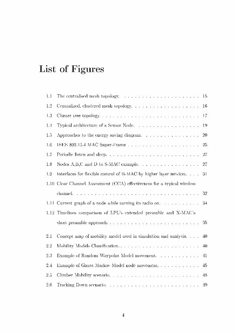
1.1 The centralised mesh topology. . . . . . . . . . . . . . . . . . . . . . 15
1.2 Centralized, clustered mesh topology. . . . . . . . . . . . . . . . . . . 16
1.3 Cluster tree topology. . . . . . . . . . . . . . . . . . . . . . . . . . . . 17
1.4 Typical architecture of a Sensor Node. . . . . . . . . . . . . . . . . . 19
1.5 Approaches to the energy saving diagram. . . . . . . . . . . . . . . . 20
1.6 IEEE 802.15.4 MAC Super-Frame . . . . . . . . . . . . . . . . . . . . 25
1.7 Periodic listen and sleep. . . . . . . . . . . . . . . . . . . . . . . . . . 27
1.8 Nodes A,B,C and D to S-MAC example. . . . . . . . . . . . . . . . . 27
1.9 Interfaces for �exible control of B-MAC by higher layer services. . . . 31
1.10 Clear Channel Assessment (CCA) e�ectiveness for a typical wireless
channel. . . . . . . . . . . . . . . . . . . . . . . . . . . . . . . . . . . 32
1.11 Current graph of a node while turning its radio on. . . . . . . . . . . 34
1.12 Timelines comparison of LPL's extended preamble and X-MAC's
short preamble approach. . . . . . . . . . . . . . . . . . . . . . . . . . 35
2.1 Concept map of mobility model used in simulation and analysis. . . . 40
2.2 Mobility Models Classi�cation. . . . . . . . . . . . . . . . . . . . . . . 40
2.3 Example of Random Waypoint Model movement. . . . . . . . . . . . 41
2.4 Example of Gauss Markov Model node movement. . . . . . . . . . . . 45
2.5 Climber Mobility scenario. . . . . . . . . . . . . . . . . . . . . . . . . 48
2.6 Tracking Down scenario. . . . . . . . . . . . . . . . . . . . . . . . . . 49
4
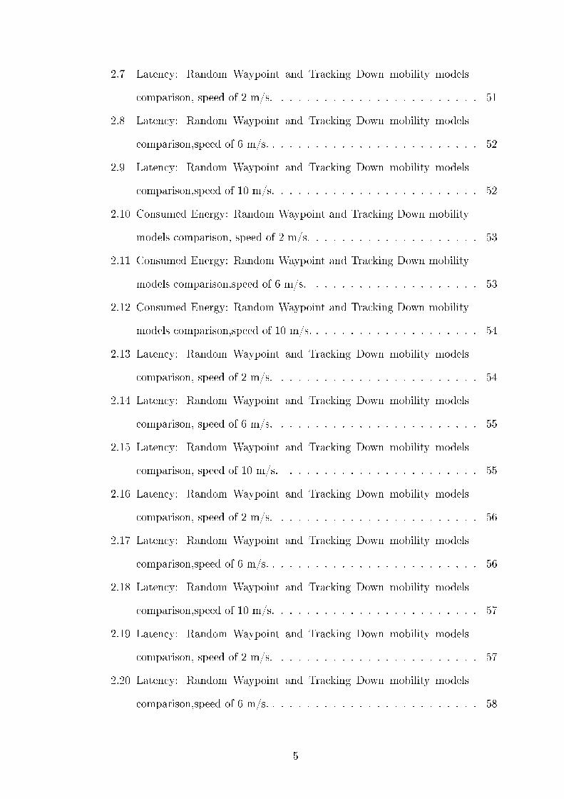
2.7 Latency: Random Waypoint and Tracking Down mobility models
comparison, speed of 2 m/s. . . . . . . . . . . . . . . . . . . . . . . . 51
2.8 Latency: Random Waypoint and Tracking Down mobility models
comparison,speed of 6 m/s. . . . . . . . . . . . . . . . . . . . . . . . . 52
2.9 Latency: Random Waypoint and Tracking Down mobility models
comparison,speed of 10 m/s. . . . . . . . . . . . . . . . . . . . . . . . 52
2.10 Consumed Energy: Random Waypoint and Tracking Down mobility
models comparison, speed of 2 m/s. . . . . . . . . . . . . . . . . . . . 53
2.11 Consumed Energy: Random Waypoint and Tracking Down mobility
models comparison,speed of 6 m/s. . . . . . . . . . . . . . . . . . . . 53
2.12 Consumed Energy: Random Waypoint and Tracking Down mobility
models comparison,speed of 10 m/s. . . . . . . . . . . . . . . . . . . . 54
2.13 Latency: Random Waypoint and Tracking Down mobility models
comparison, speed of 2 m/s. . . . . . . . . . . . . . . . . . . . . . . . 54
2.14 Latency: Random Waypoint and Tracking Down mobility models
comparison, speed of 6 m/s. . . . . . . . . . . . . . . . . . . . . . . . 55
2.15 Latency: Random Waypoint and Tracking Down mobility models
comparison, speed of 10 m/s. . . . . . . . . . . . . . . . . . . . . . . 55
2.16 Latency: Random Waypoint and Tracking Down mobility models
comparison, speed of 2 m/s. . . . . . . . . . . . . . . . . . . . . . . . 56
2.17 Latency: Random Waypoint and Tracking Down mobility models
comparison,speed of 6 m/s. . . . . . . . . . . . . . . . . . . . . . . . . 56
2.18 Latency: Random Waypoint and Tracking Down mobility models
comparison,speed of 10 m/s. . . . . . . . . . . . . . . . . . . . . . . . 57
2.19 Latency: Random Waypoint and Tracking Down mobility models
comparison, speed of 2 m/s. . . . . . . . . . . . . . . . . . . . . . . . 57
2.20 Latency: Random Waypoint and Tracking Down mobility models
comparison,speed of 6 m/s. . . . . . . . . . . . . . . . . . . . . . . . . 58
5
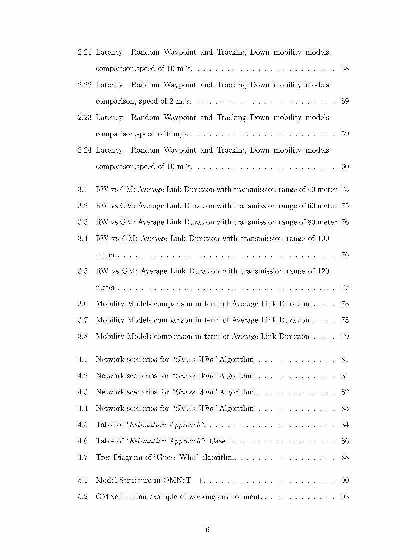
2.21 Latency: Random Waypoint and Tracking Down mobility models
comparison,speed of 10 m/s. . . . . . . . . . . . . . . . . . . . . . . . 58
2.22 Latency: Random Waypoint and Tracking Down mobility models
comparison, speed of 2 m/s. . . . . . . . . . . . . . . . . . . . . . . . 59
2.23 Latency: Random Waypoint and Tracking Down mobility models
comparison,speed of 6 m/s. . . . . . . . . . . . . . . . . . . . . . . . . 59
2.24 Latency: Random Waypoint and Tracking Down mobility models
comparison,speed of 10 m/s. . . . . . . . . . . . . . . . . . . . . . . . 60
3.1 RW vs GM: Average Link Duration with transmission range of 40 meter 75
3.2 RW vs GM: Average Link Duration with transmission range of 60 meter 75
3.3 RW vs GM: Average Link Duration with transmission range of 80 meter 76
3.4 RW vs GM: Average Link Duration with transmission range of 100
meter . . . . . . . . . . . . . . . . . . . . . . . . . . . . . . . . . . . . 76
3.5 RW vs GM: Average Link Duration with transmission range of 120
meter . . . . . . . . . . . . . . . . . . . . . . . . . . . . . . . . . . . . 77
3.6 Mobility Models comparison in term of Average Link Duration . . . . 78
3.7 Mobility Models comparison in term of Average Link Duration . . . . 78
3.8 Mobility Models comparison in term of Average Link Duration . . . . 79
4.1 Network scenarios for �Guess Who� Algorithm. . . . . . . . . . . . . . 81
4.2 Network scenarios for �Guess Who� Algorithm. . . . . . . . . . . . . . 81
4.3 Network scenarios for �Guess Who� Algorithm. . . . . . . . . . . . . . 82
4.4 Network scenarios for �Guess Who� Algorithm. . . . . . . . . . . . . . 83
4.5 Table of �Estimation Approach�. . . . . . . . . . . . . . . . . . . . . . 84
4.6 Table of �Estimation Approach�: Case 1. . . . . . . . . . . . . . . . . 86
4.7 Tree Diagram of �Guess Who� algorithm. . . . . . . . . . . . . . . . . 88
5.1 Model Structure in OMNeT++. . . . . . . . . . . . . . . . . . . . . . 90
5.2 OMNeT++ an example of working environment. . . . . . . . . . . . . 93
6
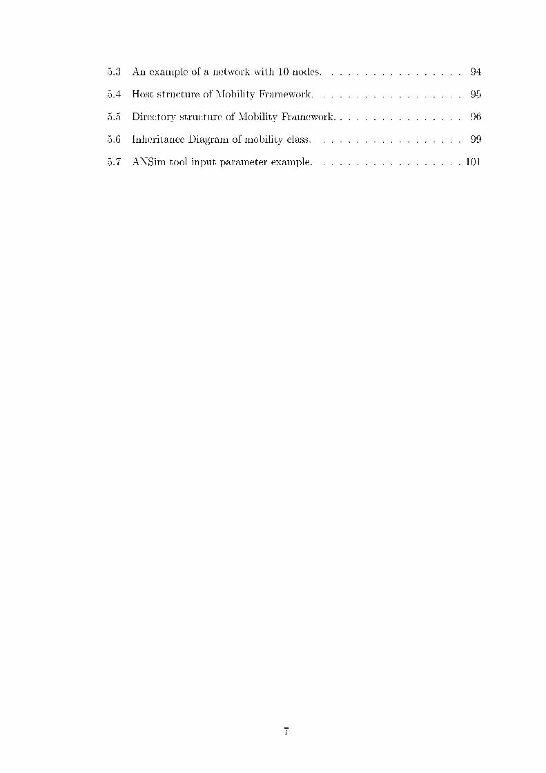
5.3 An example of a network with 10 nodes. . . . . . . . . . . . . . . . . 94
5.4 Host structure of Mobility Framework. . . . . . . . . . . . . . . . . . 95
5.5 Directory structure of Mobility Framework. . . . . . . . . . . . . . . . 96
5.6 Inheritance Diagram of mobility class. . . . . . . . . . . . . . . . . . 99
5.7 ANSim tool input parameter example. . . . . . . . . . . . . . . . . . 101
7
Introduction
In recent years, Wireless Sensor Networks (WSN) have attracted great research at-
tention thanks to the broad range of application in environment monitoring, indus-
trial process monitoring, preventative monitoring, habitat monitoring, tra�c con-
trol, emergencies, military surveillance, precise agriculture, wildlife tracking, and
many more. One peculiarity of sensor networks consists in the necessity of in-
teracting with the environment, leading these networks to be much di�erent from
conventional networks. Currently deployed sensor networks have proved good e�-
ciency in gathering information coming from sensing the physical world, where in
some cases the sensors are used to perceive the environment and act in place of the
human perceptual system, for example the auditory or tactile system.
In WSN the individual sensor nodes are generally assumed to be static. However,
some recent applications of WSN (e.g. in medical care and disaster response) make
use of mobile sensor nodes, which poses some unique challenges to WSN systems
researchers.
Most of the MAC protocols proposed for wireless sensor networks assume sen-
sors to be stationary after deployment, which usually provide very bad network
performance in scenarios involving mobile sensors. Actually, with mobile sensor ap-
plications, each communication node could be very mobile and the level of mobility
may vary in a short term base. Techniques developed for other mobile networks,
such as mobile phone or mobile ad-hoc networks can not be applicable, as in these
networks typical optimization targets of such networks are generally not main crit-
ical issues for sensor networks. Handling mobility in wireless sensor networks in an
8
energy-e�cient way is a new challenge: MAC protocols for WSN should explicitly
address the e�ects of mobile sensor nodes in the protocol design.
In this master thesis we focus on mobility characterization for mobile wireless
sensor networks. We consider three scenarios for mobility: single node (or sink)
mobility, group mobility and, both coexistent single and group mobility. Our goal
is to characterize the mobility of the agents of a WSN so that the MAC protocol
can take into account some pertinent knowledge of mobility of network agents in
the MAC access control.
Two major philosophies have been followed to characterize mobility of network
agents: �ideal� and �life-like�. Both approaches can be used for WSN. With �ideal�
approaches, mobility is characterized by simpli�ed models that have the advantage
of reducing the complexity of the model itself. Mainly, mobility is characterized by
few geometrical/statistical parameters of the mobility of the agent. Such family of
approaches cannot fully characterize the entire real behavior of the agent's mobility,
and actually it is not its goal. These models are bene�cial when a very accurate
characterization of the mobility is redundant.
With�life-like� approaches, the mobility model is derived by the observation of
real life behavior of network agents. Such family of mobility models is used by a
process that requires more accurate characterization. The two main drawbacks of
such approach are the complexity cost introduced by the higher level of accuracy
intrinsically targeted by these models and, the large observation time required to
achieve the desired accuracy of the model. In practice, depending on the complexity
budget of the above process or the time variation of the mobility itself, such models
may be suitable or not.
The work done in this master thesis is fourfold. First, we investigate how mo-
bility models can be accurately characterized. Second, we evaluated the impact of
the accuracy of the investigated mobility models on the performance of the WSN.
Third, we propose two mobility models that better �t with the speci�c investigation
scenarios chosen in this master thesis. Fourth, we propose a simple but e�cient al-
9
gorithm to estimate the best �tting mobility model for a network agent. We named
this algorithm the �Guess Who�.
The outline of the thesis is as follows:
In Chapter 1 we present a state of the art on Wireless Sensor Networks.
We illustrates the fundamentals framework features of WSNs, followed by a
general description of more common solutions which have gained a wide at-
tention in literature. We recall that the major design constraints for both
physical layer and MAC layer of the proposed solutions, has been considered
in order to limit the energy wastage of WSN agents. In fact, in some applica-
tion scenarios, the recharge of the batteries could be impossible. Sensor node
lifetime, therefore, shows a strong dependence on battery lifetime. In a multi-
hop ad hoc sensor network, each node plays the dual role of data originator
and data router. The malfunctioning of few nodes can cause signi�cant topo-
logical changes and might require re-routing of packets and re-organization
of the network. Hence, power conservation and power management take on
additional relevance. Energy conservation is not the only important design
issue in a sensor network. Framework choice is in�uenced by many factors,
including fault tolerance, scalability, production costs, operating environment,
sensor network topology, hardware constraints, and transmission channel.
In Chapter 2 we �rst present two di�erent philosophies adopted to charac-
terize mobility: `ideal' and `lifelike' approaches. Firstly we analyze the most
popular `ideal' mobility model, secondly we present our study on two partic-
ular scenarios Climbing and Tracking Down. Then, for both groups we
analyze values and �aws and we compare simulation results. We come out
with the conclusion that the adopted mode should �t with both actual mobil-
ity experienced by network agents and speci�c requirement of the process that
include for example the knowledge of mobility in the algorithm proposed.
In Chapter 3 we �rst focus on metrics for performance evaluation of mobility
10
models. Through these metrics we compare the Gauss-Markov and Random
Waypoint mobility models in order to underline their di�erences. Then we
present a stochastic properties features for a famous `ideal' mobility model.
In Chapter 4 we describe a novel algorithms that can be used to estimate
which mobility model may characterize, out of a pre-de�ned set of possible
models, the best the speci�c mobility context under observation. The best
choice depends on an utility function which characterizes the requirements in
terms of accuracy and complexity cost required by the process that will exploit
such estimation. We named this algorithm the 'Guess Who' algorithm.
In Chapter 5 overview of simulator used in this work (OMNeT++).
Finally, in Chapter 6 conclusions, future work perspectives and open prob-
lems are illustrated.
11
Chapter 1
Wireless Sensor Networks: State of
the Art
A wireless sensor network consists of a number (hundred, sometimes thousands)
sensor nodes deployed over a geographical area for monitoring physical phenomena
like temperature, humidity, vibrations or other. Sensors can automatically orga-
nize themselves and form ad hoc multi-hop networks for peer to peer, local gossip or
convergast communications [3]. Several applications for wireless sensor networks are
imaginable so medicine, agriculture, environment, military, inventory monitoring, in-
trusion detection, motion tracking, machine malfunction, toys and many others. In
the medical �eld sensor networks can be used to remotely and unobtrusively mon-
itor physiological parameters of patients such as heartbeat or blood pressure, and
report to the hospital when some parameters are altered. In agriculture, they can be
used to monitor climatic conditions of di�erent zones of a large cultivated area and
calculate di�erent water or chemicals needs. Pollution detection systems can also
bene�t from sensor networks. Sensors can monitor the current levels of polluting
substances in a town or a river and identify the source of anomalous situations, if
any. Similar detection systems can be employed to monitor rain and water levels and
prevent �ooding, �re or other natural disasters. Another possible application that
was recently experimented is the monitoring of animal species and collection of data
12
concerning their habits, population, or position. Sensors can be deployed to contin-
uously report environmental data for long periods of time. This is a very important
improvement with respect to the previous operating conditions where humans had
to operate in the �elds and periodically take manual measurements resulting in
fewer data, higher errors, higher costs and non negligible interference with life con-
ditions of the observed species. In structure health monitoring applications, sensor
networks are deployed on structures such as bridges, buildings, aircrafts, rockets or
other military equipment requiring continuous monitoring to ensure reliability and
safety. The military can take advantage of sensor network technology too. They
can deploy such networks behind enemy lines and observe movements/presence of
troops and/or collect geographical information on the deployment area. Other possi-
ble �elds include home/o�ce automation, inventory monitoring, intrusion detection,
motion tracking, machine malfunctions.
1.1 Self-Organization, Topology and Connectivity
Wireless sensor devices are equipped with a radio transceiver and a set of transceiver
through which they acquire information about the surrounding environment. In ad-
dition a power source supplies the energy needed by the device to perform the pro-
grammed task. In most cases WSNs should operate in an unattended environment
where long lifetime feature is needed, therefore WSN should have the characteristics
for �self-organization� [1]. A system is self-organizing if a collection of units coordi-
nate themselves to form a system that adapts itself in order to achieve a goal more
e�ciently. Others system features are the units capacity for responding to local
stimuli or for acting together to achieve a division of a labour. The overall system
adapts to achieve a goal or the de�ned goals more e�ciently.
The goal of WSNs can be summarized as to detect or track events with mini-
mized errors while at the same time minimizing the power consumption and required
communication. A WSN is de�ned as �organized�, if it can achieve the goal of mini-
13
mization of the weighted sum of detecting or tracking error, power consumption and
communication. The nodes organization can be achieved with �at or hierarchical
topology. In the latter case a subset of nodes in the network would be selected as
a Connected Dominant Set (CDS) and the network is divided into clusters. The
node in the connected dominant set may act as cluster heads and the other nodes
act as clusters members. Once the clusters are formed can be assigned a time-slots,
a frequency bands or spread spectrum codes between the cluster. The problem in
the hierarchical self-organization is the overhead introduced and energy waste for
building-up the cluster. In a hierarchical self-organization scenario the global topol-
ogy information is not available and each node needs to make the decision if it is
going to be in the CDS locally. The characteristics of the network have an essential
in�uence on the trade-o� between the cost and the gain. In fact, the decision to
apply logical hierarchical topology in a network depends on whether the cost spent
on building and maintaining the topology can be compensated by the gain in the
steady state.
The nodes organization can be achieved with �at topology where an important
issue for self-organization is the sleeping schedule. For energy conservation reasons
the sensor nodes must go periodically to sleep for reducing energy waste due to the
idle listening. Therefore nodes need to know when to transmit so that their receiver
would be awake. This can be achieved through MAC protocol design for WSNs, in
particular it is possible single out two means. The �rst one is to synchronize the
sleep schedule of neighbor nodes. This techniques is applied in S-MAC [6] and T-
MAC [9]. Another method is proposed by B-MAC [7] where a transmitter wakes-up
the receiver by sending a preamble that is longer than its sleeping period; than it
sends data. In �at topology usually the MAC is contention based like in the carrier
sense multiple access with collision avoidance (CSMA\CA).
The topology control [1] design is a key element since the topology sets the frame-
work on which the system is built. The choice of the topology and the way to control
it depend on several factors such as the capacity of the network, the connectivity
14
and the correct combination of QoS and the power consumption. In this context
the choice of the topology and related control can help to �nd better trade-o�s. For
example instead of transmitting at maximal power, nodes in a wireless multi-hop
network collaboratively determine their transmission power and de�ne the network
topology by setting their proper optimized neighbor relations. In order to de�ne
more precisely a topology the distinction can be re�ned considering the capabil-
ity of the system to allow mesh networking to perform peer-to-peer communication
also called mesh communication which is opposed to centralized or star topology
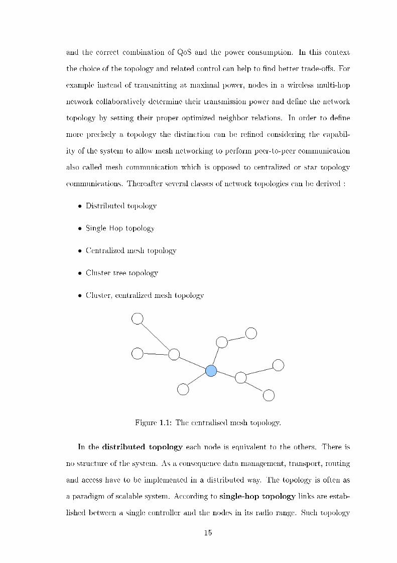
communications. Thereafter several classes of network topologies can be derived :
• Distributed topology
• Single Hop topology
• Centralized mesh topology
• Cluster tree topology
• Cluster, centralized mesh topology
Figure 1.1: The centralised mesh topology.
In the distributed topology each node is equivalent to the others. There is
no structure of the system. As a consequence data management, transport, routing
and access have to be implemented in a distributed way. The topology is often as
a paradigm of scalable system. According to single-hop topology links are estab-
lished between a single controller and the nodes in its radio range. Such topology
15
is well suited when the number of nodes does not exceed 10's of nodes and ideally
when a power line plugged device id available to act as the controller. The
centralized mesh topology shown in Figure 1.1 extends the range of the single
hop topology allowing multi-hop transmission in a centralized way. It is based on a
tree structure, it is rooted at the controller and the links between nodes represent
the tree branches. The controller is on charge of the handling of the tree and the
allocation of the resource along the tree. In extended range contexts with dispersed
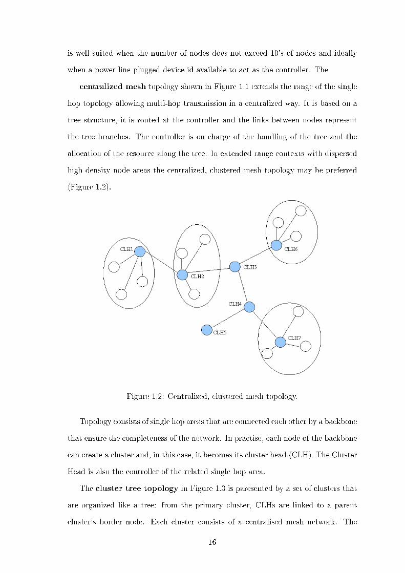
high density node areas the centralized, clustered mesh topology may be preferred
(Figure 1.2).
Figure 1.2: Centralized, clustered mesh topology.
Topology consists of single hop areas that are connected each other by a backbone
that ensure the completeness of the network. In practise, each node of the backbone
can create a cluster and, in this case, it becomes its cluster head (CLH). The Cluster
Head is also the controller of the related single hop area.
The cluster tree topology in Figure 1.3 is paresented by a set of clusters that
are organized like a tree: from the primary cluster, CLHs are linked to a parent
cluster's border node. Each cluster consists of a centralised mesh network. The
16
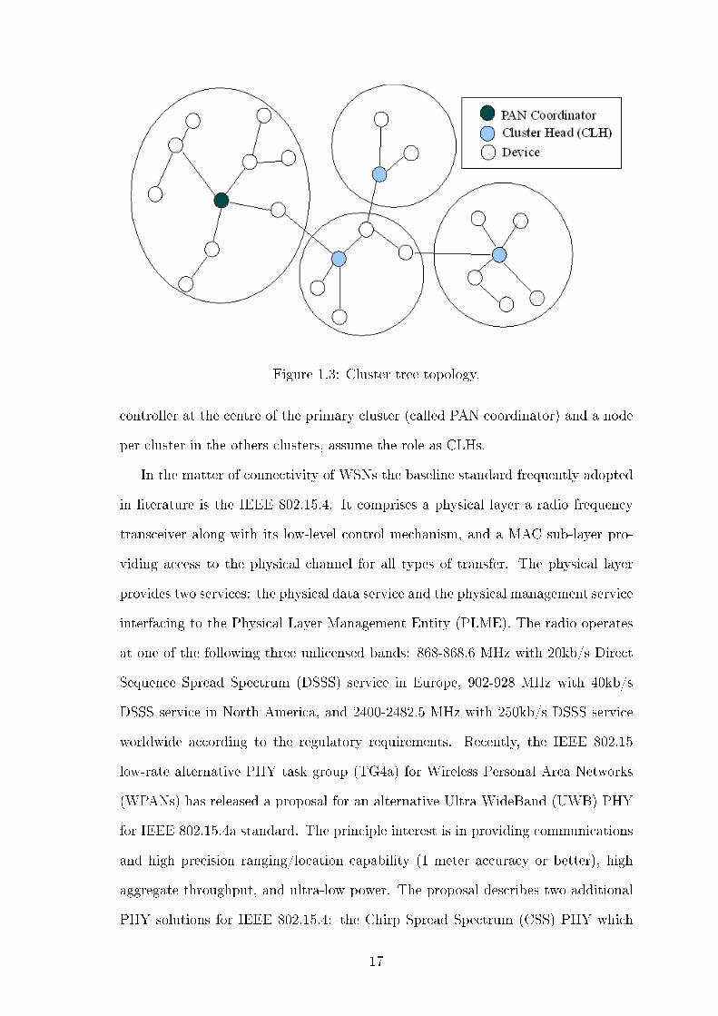
Figure 1.3: Cluster tree topology.
controller at the centre of the primary cluster (called PAN coordinator) and a node
per cluster in the others clusters, assume the role as CLHs.
In the matter of connectivity of WSNs the baseline standard frequently adopted
in literature is the IEEE 802.15.4. It comprises a physical layer a radio frequency
transceiver along with its low-level control mechanism, and a MAC sub-layer pro-
viding access to the physical channel for all types of transfer. The physical layer
provides two services: the physical data service and the physical management service
interfacing to the Physical Layer Management Entity (PLME). The radio operates
at one of the following three unlicensed bands: 868-868.6 MHz with 20kb/s Direct
Sequence Spread Spectrum (DSSS) service in Europe, 902-928 MHz with 40kb/s
DSSS service in North America, and 2400-2482.5 MHz with 250kb/s DSSS service
worldwide according to the regulatory requirements. Recently, the IEEE 802.15
low-rate alternative PHY task group (TG4a) for Wireless Personal Area Networks
(WPANs) has released a proposal for an alternative Ultra WideBand (UWB) PHY
for IEEE 802.15.4a standard. The principle interest is in providing communications
and high precision ranging/location capability (1 meter accuracy or better), high
aggregate throughput, and ultra-low power. The proposal describes two additional
PHY solutions for IEEE 802.15.4: the Chirp Spread Spectrum (CSS) PHY which
17
uses a spreading mechanism to provide approximately 14 MHz bandwidth at 1Mbps
(250kbps optional) and the ultra wide band (UWB) PHY that uses very short du-
ration impulses to generate its approximately 500/1500 MHz bandwidth with 842
kbps (several others optional).
1.2 Energy Conservation
Typical architecture of a sensor node is shown in Figure 1.4 [2], it is composed of
four main components:
• Sensing unit including one or more sensors (with associated analog-to-digital
converters) for data acquisition
• Processing unit including a micro-controller and memory for local data pro-
cessing
• Radio equipment for wireless data communication
• Power supply unit
Depending on the speci�c application, sensor nodes may also include additional
components such as a location �nding system for determining their position, a mo-
bilizer to change their location or con�guration, and so on.
Analyzing the power characteristics of a sensor node we can remark that radio
equipment implies much higher energy consumption than the processing unit [4]. It
has been shown that transmitting one bit may consume as much as executing a few
thousands instructions. Therefore, communication must be traded for computation.
Moreover the radio energy consumption is of the same order in the reception, trans-
mission, and idle states, while the power consumption drops of at least one order
of magnitude in the sleep state. Therefore, the radio should be put to sleep (or
turned o�) whenever possible. Depending on the speci�c application, the sensing
18
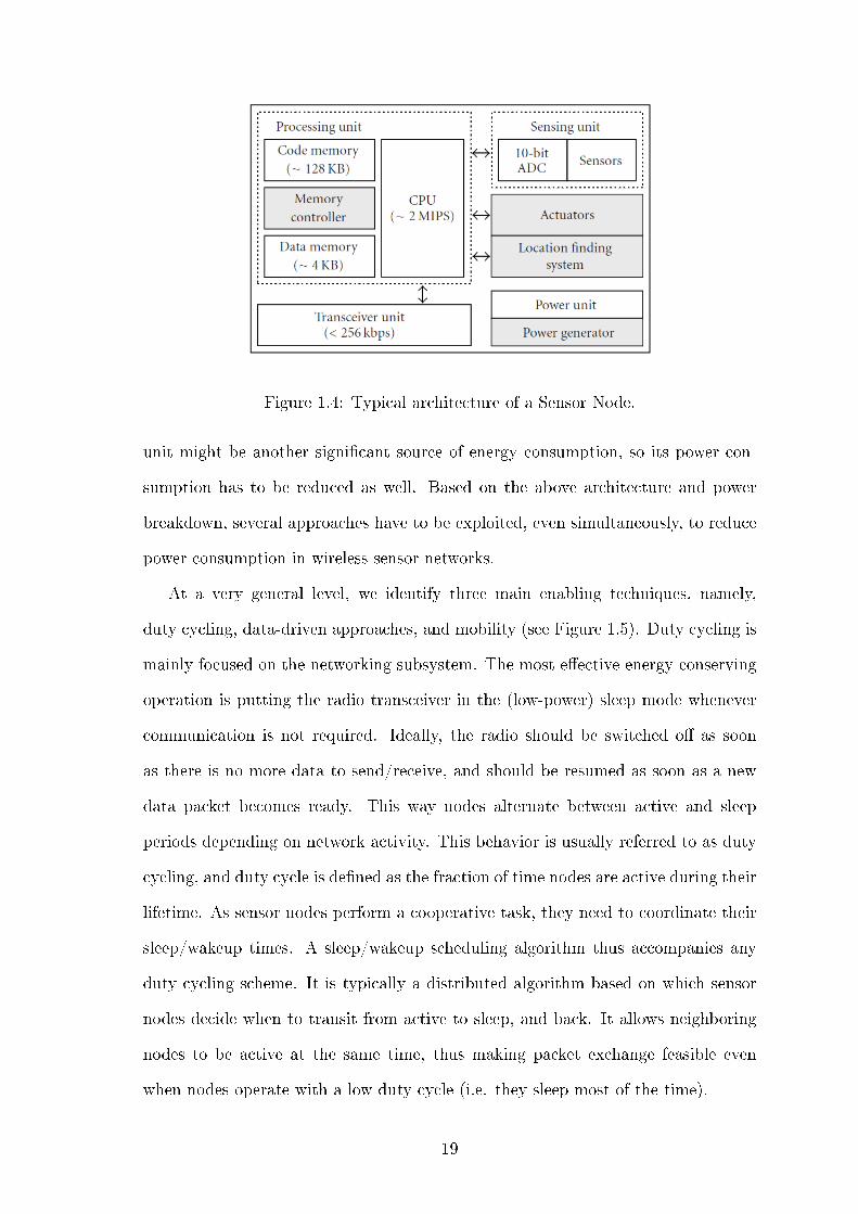
Figure 1.4: Typical architecture of a Sensor Node.
unit might be another signi�cant source of energy consumption, so its power con-
sumption has to be reduced as well. Based on the above architecture and power
breakdown, several approaches have to be exploited, even simultaneously, to reduce
power consumption in wireless sensor networks.
At a very general level, we identify three main enabling techniques, namely,
duty cycling, data-driven approaches, and mobility (see Figure 1.5). Duty cycling is
mainly focused on the networking subsystem. The most e�ective energy-conserving
operation is putting the radio transceiver in the (low-power) sleep mode whenever
communication is not required. Ideally, the radio should be switched o� as soon
as there is no more data to send/receive, and should be resumed as soon as a new
data packet becomes ready. This way nodes alternate between active and sleep
periods depending on network activity. This behavior is usually referred to as duty
cycling, and duty cycle is de�ned as the fraction of time nodes are active during their
lifetime. As sensor nodes perform a cooperative task, they need to coordinate their
sleep/wakeup times. A sleep/wakeup scheduling algorithm thus accompanies any
duty cycling scheme. It is typically a distributed algorithm based on which sensor
nodes decide when to transit from active to sleep, and back. It allows neighboring
nodes to be active at the same time, thus making packet exchange feasible even
when nodes operate with a low duty cycle (i.e. they sleep most of the time).
19
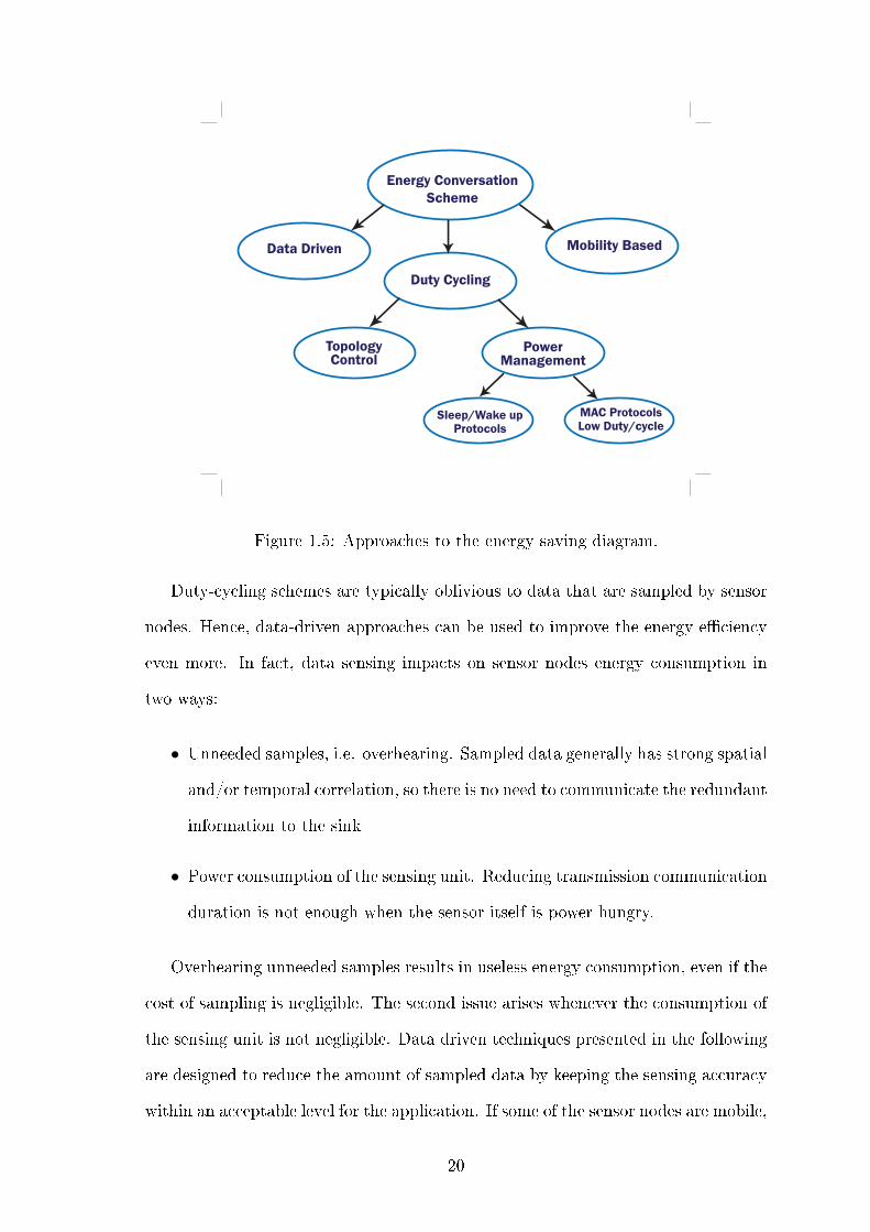
Figure 1.5: Approaches to the energy saving diagram.
Duty-cycling schemes are typically oblivious to data that are sampled by sensor
nodes. Hence, data-driven approaches can be used to improve the energy e�ciency
even more. In fact, data sensing impacts on sensor nodes energy consumption in
two ways:
• Unneeded samples, i.e. overhearing. Sampled data generally has strong spatial
and/or temporal correlation, so there is no need to communicate the redundant
information to the sink
• Power consumption of the sensing unit. Reducing transmission communication
duration is not enough when the sensor itself is power hungry.
Overhearing unneeded samples results in useless energy consumption, even if the
cost of sampling is negligible. The second issue arises whenever the consumption of
the sensing unit is not negligible. Data driven techniques presented in the following
are designed to reduce the amount of sampled data by keeping the sensing accuracy
within an acceptable level for the application. If some of the sensor nodes are mobile,
20
mobility can �nally be used as a tool for reducing energy consumption (beyond duty
cycling and data-driven techniques). In a static sensor network packets coming from
sensor nodes follow a multi-hop path towards the sink. Thus, a few paths can be
more loaded than others; nodes closer to the sink have to relay more packets so
that they are more subject to premature energy depletion (funneling e�ect). If
some of the nodes (including, possibly, the sink) are mobile, the tra�c �ow can
be altered if mobile devices are responsible for data collection directly from static
nodes. Ordinary nodes wait for the passage of the mobile device and route messages
towards it, so that the communications take place in proximity (directly or at most
with a limited multi-hop traversal). As a consequence, ordinary nodes can save
energy because path length, contention and forwarding overheads are reduced as
well. In addition, the mobile device can visit the network in order to spread more
uniformly the energy consumption due to communications.
When the cost of mobilizing sensor nodes is prohibitive, the usual approach is
to �attach� sensor nodes to entities that will move around the sensing �eld anyway,
such as buses or animals. All of the schemes described in the literature fall under
one of the three general approaches we have presented.
1.3 MAC Protocols
Among MAC protocols available in the literature in the following subsections we
will focus on one of the most popular class of MAC protocol for power management:
contention based MAC protocols with low duty-cycle scheme. We focus own attention
on the following protocols:
• IEEE 802.15.4
• S-MAC
• B-MAC
• X-MAC
21
IEEE 802.15.4 is a standard for low-rate, low-power Personal Area Networks
(PANs). A PAN is formed by one PAN coordinator which manages the whole net-
work, and, optionally, by one or more coordinators which manage subsets of nodes
in the network. Other (ordinary) nodes must associate with a (PAN) coordinator
in order to communicate. The supported network topologies are star (single-hop),
cluster-tree and mesh (multi-hop). The IEEE 802.15.4 standard supports two dif-
ferent channel access methods: a beacon enabled mode and a non-beacon enabled
mode.
The beacon enabled mode provides an energy management mechanism based
on a duty cycle. Speci�cally, it uses a super-frame structure which is bounded by
beacons-special synchronization frames generated periodically by coordinator nodes.
Each super-frame consists of an active period and an inactive period. In the active
period devices communicate with the coordinator they associated with. The active
period can be further divided in a contention access period (CAP) and a collision free
period (CFP). During the CAP a slotted CSMA/CA algorithm is used for channel
access, while in the CFP a number of guaranteed time slots (GTSs) can be assigned
to individual nodes. During the inactive period devices enter a low power state to
save energy.
In the non-beacon enabled mode there is no super-frame structure, i.e. nodes are
always in the active state and use an unslotted CSMA/CA algorithm for channel
access and data transmission. In this case, energy conservation is up to the above
layers.
IEEE 802.15.4 beacon-enabled mode is suitable for single-hop scenarios. How-
ever the beacon-based duty-cycle scheme has to be extended for multi-hop networks.
In [1] authors propose a maximum delay bound wakeup scheduling speci�cally tai-
lored to IEEE 802.15.4 networks. The sensor network is assumed to be organized as
a cluster tree. An optimization problem is formulated in order to maximize network
lifetime while satisfying latency constraints. The optimal operating parameters for
single coordinators are then obtained. Therefore, an additional extended synchro-
22
nization scheme is used for inter-cluster communication.
A well-known MAC protocol for multi-hop sensor networks is S-MAC (Sensor-
MAC) [6], which adopts a scheduled rendez-vous communication scheme. Nodes
exchange SYNC packets to coordinate their sleep/wakeup periods. Every node can
establish its own schedule or follow the schedule of a neighbor by means of a random
distributed algorithm. Nodes using the same schedule form a virtual cluster (VC).
Nodes that are at the border of two VCs may eventually follow the schedules of both
the VCs so to behave link a �bridge node�. The channel access time is split in two
parts: wake up/listen period and a sleep period. In the beginning of the wake up
period nodes exchange synchronization packets (SYNC) and special control packets
for collision avoidance. In the remainder of the wake up period the actual data
transfer takes place. The sender and the destination node are awake and talk to
each other. Nodes not concerned with the communication process can sleep until
the next listen period. To avoid high latencies in multi-hop environments S-MAC
uses an adaptive listening scheme. A node overhearing its neighbor's transmissions
wakes up at the end of the transmission for a short period of time. If the node is
the next hop of the transmitter, the neighbor can send immediately the packet to it
without waiting for the next schedule. The parameters of the protocol, i.e. the listen
and the sleep periods, are constants and cannot be varied after the deployment of
the nodes.
One of the most popular contention-based MAC protocols is B-MAC (Berkeley
MAC) [7], a low-complexity and low power MAC protocol. The goal of B-MAC is
to provide a few core functionalities and an energy e�cient mechanisms for channel
access. First, B-MAC implements basic channel access control features: a back-
o� scheme, an accurate channel estimation facility and optional acknowledgements.
Second, to achieve a low duty cycle it uses an asynchronous sleep/wake scheme based
on periodic listening called Low Power Listening (LPL). Nodes periodically wake-up
to check the channel for activity. The period between consecutive wakes-up is called
check interval. After waking up, nodes remain active for a wake up time, in order
23
to properly detect eventual ongoing transmissions. While the wake up time is �xed,
the check interval can be speci�ed by the application. B-MAC packets are made up
of a long preamble and a payload. The preamble duration is at least equal to the
check interval so that each node can always detect an ongoing transmission during
its check interval. This approach does not require nodes to be synchronized. In fact,
when a node detects channel activity, it just remains active and receives �rst the
preamble and then the payload.
The X-MAC Protocol [8] like the B-MAC employs an extended preamble and
preamble sampling. While this �Low Power Listening� approach is simple, asyn-
chronous and energy-e�cient, the long preamble introduces excess latency at each
hop, is suboptimal in terms of energy consumption and su�ers from excess energy
consumption at non-target receivers. X-MAC proposes solutions to each of these
problems by employing a shortened preamble approach that retains the advantages
of low power listening, namely low power communication, simplicity and a decou-
pling of transmitter and receiver sleep schedules.
1.3.1 IEEE 802.15.4 MAC Protocol
With respect to MAC, devices compliant to the IEEE 802.15.4 [5] standard can be
divided into: Reduced Function Devices (RFDs) and Full Function Devices (FFDs).
FFDs are equipped with a full set of MAC layer functions, which enables them to
act as a network coordinator or a network end-device. When acting as a network
coordinator, FFDs send beacons that provide synchronization, communication and
network join services. RFDs can only act as end-devices and are equipped with
sensors/actuators like transducers, light switches, lamps, etc. RFDs may only in-
teract with a single FFD. Two main types of network topology are considered in
IEEE 802.15.4, namely, the star topology and the peer-to-peer topology. In the
star topology, a master-slave network model is adopted. A FFD takes up the role of
PAN coordinator; the other nodes can be RFDs or FFDs and will only communicate
24
with the PAN coordinator. In the peer-to-peer topology, a FFD can talk to other
FFDs within its radio range and can relay messages to other FFDs outside of its
radio coverage through an intermediate FFD, forming a multi-hop network. A PAN
coordinator is selected to administer network operation.
The Persona Area Network (PAN) coordinator may work in two modalities with
a super-frame or without it. In the �rst case it starts the super-frame with a beacon
serving for synchronization purposes as well as to de�ne the super-frame structure
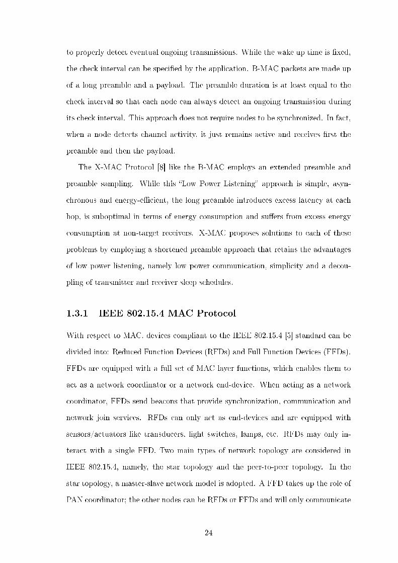
and send control information to the PAN. The super-frame, structure shown on Fig-
ure 1.6 is divided into an active and an inactive portion (where the PAN coordinator
may go to sleep and save energy).
Figure 1.6: IEEE 802.15.4 MAC Super-Frame
The active portion is divided into �xed size slots and contains a Contention
Access Period (CAP), where nodes compete for channel access using a slotted
CSMA/CA protocol, and a Contention Free Period (CFP), where nodes transmit
without contending for the channel in Guaranteed Time Slots (GTS) assigned and
administered by the PAN coordinator.
When an end-device needs to send data to a coordinator not during GTS period
it must wait for the beacon to synchronize and later contend for channel access.
On the other hand, communication from a coordinator to an end-device is indirect.
In fact the coordinator stores the message and announces pending delivery in the
beacon. End-devices usually sleep most of the time and wake up periodically to see
if they have to receive some messages from the coordinator by waiting for the bea-
25
con. When they notice that a message is available, they request it explicitly during
the CAP. When a coordinator wishes to talk to another coordinator it must �rst
synchronize with its beacon and then act as an end-device. The other option for
PAN communication is to do without a super-frame. The PAN coordinator never
sends beacons and communication follows the basis of unslotted CSMA/CA.
The coordinator's radio is always on and ready to receive data from an end-device
while data transfer in the opposite direction is poll-based: the end device period-
ically wakes up and polls the coordinator for pending messages. The coordinator
then sends these messages or signals that none is available. Coordinator to co-
ordinator communication poses no problems since both nodes are active all the
time. In addition to data transfer, the MAC layer o�ers channel scan and associ-
ation/disassociation functionalities. The scan procedure involves scanning several
logical channels by sending a beacon request message and listening (active scan, for
FFDs) or just listening (passive scan, for RFDs) for beacons in order to locate ex-
isting PANs and coordinators. Higher layers decide which PAN to join and later ask
the MAC layer to start an association procedure for the selected PAN. This involves
sending a request to a coordinator and waiting for the corresponding acceptance
message. If accepted in the PAN, the node receives a 16-bit �short� address that it
may use later in place of the 64-bit �extended� IEEE address.
1.3.2 S-MAC
S-MAC [6] is a protocol speci�cally designed for WSNs; it reduce energy consump-
tion while supporting good scalability and collision avoidance. The protocol tries to
reduce energy consumption by three major functions:
1. Periodic listen and sleep
2. Collision and overhearing avoidance
3. Message passing
26
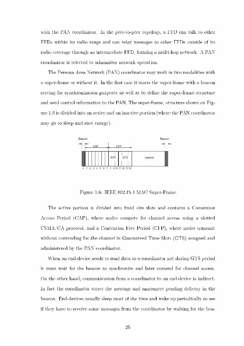
With regard to periodic listen and sleep it is not necessary to keep nodes listening
all the time. S-MAC reduces the listen time by putting nodes into periodic sleep
state. The basic scheme is shown in Figure 1.7. Each node sleeps for some time,
and then wakes up and listens to see if any other node wants to talk to it. When
asleep, the node turns o� its radio, and sets a timer to awake itself later.
Figure 1.7: Periodic listen and sleep.
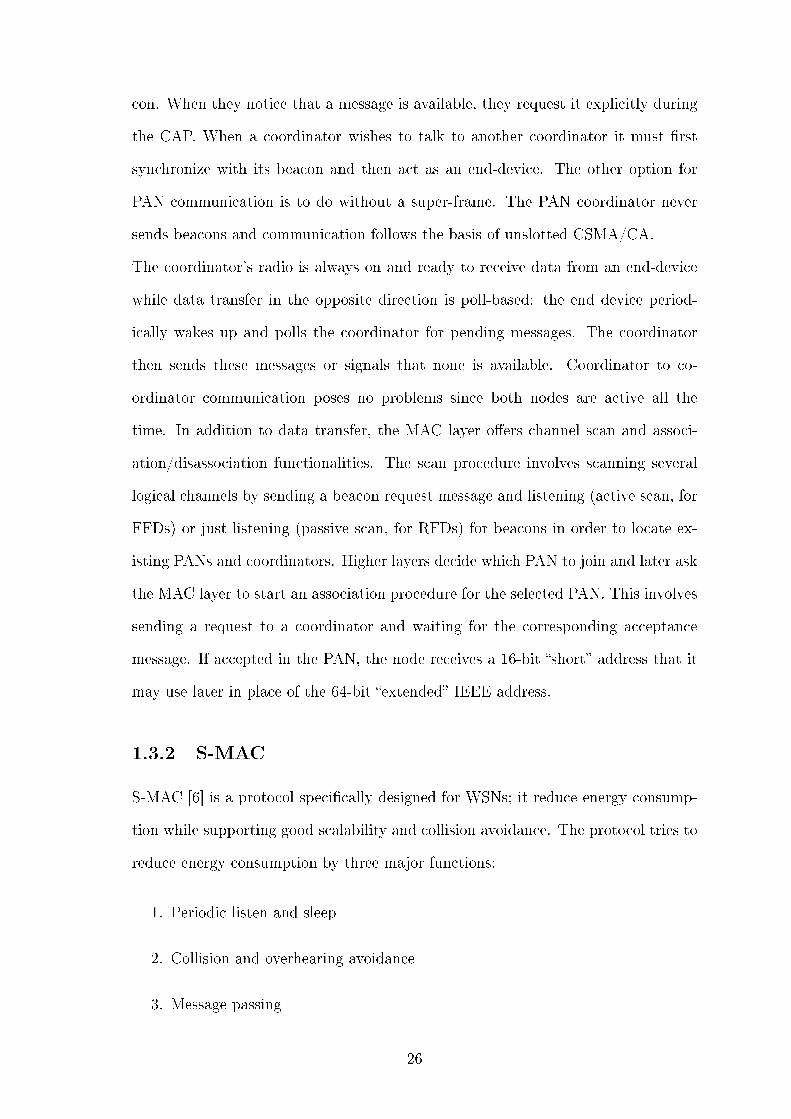
All nodes are free to choose their own listen/sleep schedule. However, to reduce
control overhead, neighboring nodes synchronize together. That is, they listen at
the same time and go to sleep at the same time. It should be noticed that not all
neighboring nodes can synchronize together in a multi-hop network. Two neigh-
boring nodes A and B may have di�erent schedules if they must synchronize with
di�erent nodes, C, and D, respectively. Nodes exchange their schedules by period-
ically broadcasting a SYNC packet to their immediate neighbors. A node talks to
its neighbors at their scheduled listen time, thus ensuring that all neighboring nodes
can communicate even if they have di�erent schedules.
Figure 1.8: Nodes A,B,C and D to S-MAC example.
In Figure 1.8, for example, if node A wants to talk to node B, it waits until B is
listening. The period for a node to send a SYNC packet is called the synchronization
period. If multiple neighbors want to talk to a node at the same time, they will try
to send when the node starts listening. In this case, they need to contend for the
medium. S-MAC follows a procedure including virtual and physical carrier sense
27
and the RTS/CTS handshake for avoiding the hidden terminal problem. Before
each node starts its periodic listen and sleep, it needs to choose a schedule and
exchange it with its neighbors. Each node maintains a schedule table that stores
the schedules of all its known neighbors. Following step show the procedures of a
node for choosing to choose its schedule and establish its schedule table.
1. A node �rst listens for a �xed amount of time, which is at least the synchroniza-
tion period. If it does not hear a schedule from another node, it immediately
chooses its own schedule and starts to follow it. Meanwhile, the node tries to
announce the schedule by broadcasting a SYNC packet. Broadcasting a SYNC
packet follows the normal contention procedure. The randomized carrier sense
time reduces the chance of collisions of SYNC packets.
2. If the node receives a schedule from a neighbor before choosing or announcing
its own schedule, it follows that schedule. Then the node will try to announce
its schedule at its next scheduleding listen time.
3. There are two cases in case that a node receives a di�erent schedule after it
chooses and announces its own schedule. If the node has no neighbors it will
discard its current schedule and follow the new one. If the node already follows
a the schedule of its neighbors. It adopts both schedules by waking up at the
listen intervals of the two schedules (thus increasing energy consumption).
The scheme of periodic listen and sleep is able to signi�cantly reduce the time
spent on idle listening when tra�c load is light. However, when a sensing event
indeed happens, it is desirable that the sensing data can be passed through the
network without too much delay. When each node strictly follows its sleep schedule,
there is a potential delay on each hop, whose average value is proportional to the
length of the frame. We therefore introduce a mechanism to switch the nodes from
the low-duty-cycle mode to a more active mode in this case. S-MAC proposes an
important technique, called adaptive listen, to reduce the latency caused by the
periodic sleep of each node in a multi-hop network.
28
The basic idea is to let the node who overhears its neighbor's transmissions
(ideally only RTS or CTS) wake up for a short period of time at the end of the
transmission. In this way, if the node is the next-hop node, its neighbor is able to
immediately pass data to it instead of waiting for its scheduled listen time. If the
node does not receive anything during the adaptive listening, it will go back to sleep
until its next scheduled listen time.
Another important feature of S-MAC is the concept of message-passing where
long messages are divided into frames and sent in a burst. With this technique, one
may achieve energy savings by minimizing communication overhead at the expense
of unfairness in medium access. Periodic sleep may result in high latency especially
for multi-hop routing algorithms, since all immediate nodes have their own sleep
schedules. The latency caused by periodic sleeping is called sleep delay [6].
Unlike clustering protocols, S-MAC does not require coordination through clus-
ter heads. Nodes form virtual clusters by sharing common schedules, and they
communicate directly with a peer-to-peer topology. One advantage of this loose
coordination is that it can be more robust to topology change than cluster-based
approaches. The downside of the scheme is the increased latency due to the peri-
odic sleeping. Furthermore, the delay can accumulate on each hop. S-MAC with the
low-duty-cycle operation and the contention mechanism during each listen interval,
e�ectively addresses the energy waste due to idle listening and collisions. Moreover,
in a network where all nodes can hear each other, the node who starts �rst will pick
up a schedule �rst, and its broadcast will synchronize all its peers on its schedule.
If two or more nodes start �rst at the same time, they will �nish initial listening at
the same time, and will choose the same schedule independently. No matter which
node sends out its SYNC packet �rst (wins the contention), it will synchronize the
rest of the nodes. However it is possible that two nodes may independently assign
schedules if they cannot hear each other in a multi-hop network. In this case, those
nodes on the border of two schedules will adopt both. For example, nodes A and B
in Figure 1.8 will wake up at the listen time of both schedules. In this way, when
29
a border node sends a broadcast packet, it only needs to send it once. The disad-
vantage is that these border nodes have less time to sleep and consume more energy
than others.
1.3.3 B-MAC
B-MAC [7] is a carrier sense medium access protocol for wireless sensor networks
that provides a �exible interface to obtain ultra low power operation, e�ective colli-
sion avoidance and high channel utilization. B-MAC employs an adaptive preamble
sampling scheme to reduce duty cycle and minimize idle listening. B-MAC pro-
tocol contains a small core of media access functionality. In fact B-MAC uses
clear channel assessment (CCA) and packet backo�s for channel arbitration, link
layer acknowledgments for reliability, and Low Power Listening (LPL) for low power
communication. B-MAC is only a link protocol, with network services like orga-
nization, synchronization, and routing built above its implementation. Although
B-MAC neither provides multi-packet mechanisms like hidden terminal support or
message fragmentation nor enforces a particular low power policy, B-MAC has a set
of interfaces that allow services to tune its operation (see Figure 1.9) in addition to
the standard message interfaces.
These interfaces allow network services to adjust BMAC's mechanisms, includ-
ing CCA, acknowledgments, back-o�s, and LPL. By exposing a set of con�gurable
mechanisms, protocols built on B-MAC make local policy decisions to optimize
power consumption, latency, throughput, fairness or reliability. For e�ective colli-
sion avoidance, a MAC protocol must be able to accurately determine if the channel
is clear, referred to as Clear Channel Assessment (CCA). Since the ambient noise
changes depending on the environment, B-MAC employs software automatic gain
control for estimating the noise �oor. Signal strength samples are taken at times
when the channel is assumed to be free-such as immediately after transmitting a
packet or when the data path of the radio stack is not receiving valid data. Samples
30
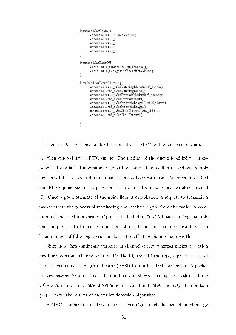
Figure 1.9: Interfaces for �exible control of B-MAC by higher layer services.
are then entered into a FIFO queue. The median of the queue is added to an ex-
ponentially weighted moving average with decay α. The median is used as a simple
low pass �lter to add robustness to the noise �oor estimate. An α value of 0.06
and FIFO queue size of 10 provided the best results for a typical wireless channel
[7]. Once a good estimate of the noise �oor is established, a request to transmit a
packet starts the process of monitoring the received signal from the radio. A com-
mon method used in a variety of protocols, including 802.15.4, takes a single sample
and compares it to the noise �oor. This threshold method produces results with a
large number of false negatives that lower the e�ective channel bandwidth.
Since noise has signi�cant variance in channel energy whereas packet reception
has fairly constant channel energy. On the Figure 1.10 the top graph is a trace of
the received signal strength indicator (RSSI) from a CC1000 transceiver. A packet
arrives between 22 and 54ms. The middle graph shows the output of a thresholding
CCA algorithm. 1 indicates the channel is clear, 0 indicates it is busy. The bottom
graph shows the output of an outlier detection algorithm.
B-MAC searches for outliers in the received signal such that the channel energy
31
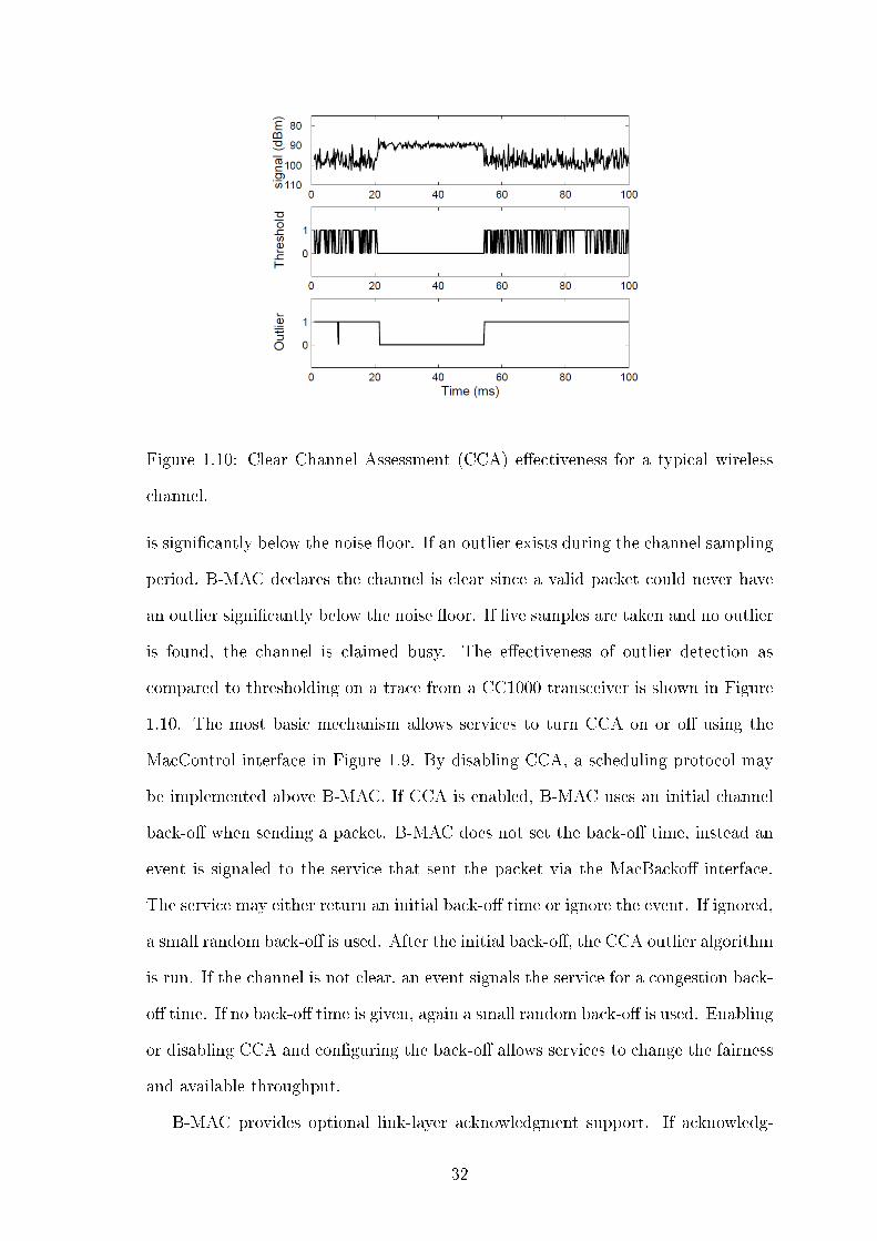
Figure 1.10: Clear Channel Assessment (CCA) e�ectiveness for a typical wireless
channel.
is signi�cantly below the noise �oor. If an outlier exists during the channel sampling
period, B-MAC declares the channel is clear since a valid packet could never have
an outlier signi�cantly below the noise �oor. If �ve samples are taken and no outlier
is found, the channel is claimed busy. The e�ectiveness of outlier detection as
compared to thresholding on a trace from a CC1000 transceiver is shown in Figure
1.10. The most basic mechanism allows services to turn CCA on or o� using the
MacControl interface in Figure 1.9. By disabling CCA, a scheduling protocol may
be implemented above B-MAC. If CCA is enabled, B-MAC uses an initial channel
back-o� when sending a packet. B-MAC does not set the back-o� time, instead an
event is signaled to the service that sent the packet via the MacBacko� interface.
The service may either return an initial back-o� time or ignore the event. If ignored,
a small random back-o� is used. After the initial back-o�, the CCA outlier algorithm
is run. If the channel is not clear, an event signals the service for a congestion back-
o� time. If no back-o� time is given, again a small random back-o� is used. Enabling
or disabling CCA and con�guring the back-o� allows services to change the fairness
and available throughput.
B-MAC provides optional link-layer acknowledgment support. If acknowledg-
32
ments are enabled, B-MAC immediately transfers an acknowledgment code after re-
ceiving a unicast packet. If the transmitting node receives the acknowledgment, an
acknowledge bit is set in the sender's transmission message bu�er. B-MAC duty cy-
cles the radio through periodic channel sampling called Low Power Listening (LPL).
B-MAC technique is similar to preamble sampling in Aloha but tailored to di�erent
radio characteristics. Each time the node wakes up, it turns on the radio and checks
for activity. If activity is detected, the node powers up and stays awake for the time
required to receive the incoming packet. After reception, the node returns to sleep.
If no packet is received (a false positive), a timeout forces the node back to sleep.
Accurate Clear Channel Assessment (CCA) is critical to achieving low power
operation with this method. The noise �oor estimation of B-MAC is use not only
for �nding a clear channel on transmission but also for determining if the channel is
active during LPL. False positives in the CCA algorithm (such as those caused by
thresholding) severely a�ect the duty cycle of LPL due to increased idle listening.
To reliably receive data, the preamble length is matched to the interval that the
channel is checked for activity. If the channel is checked every 100 ms, the preamble
must be at least 100 ms long for a node to wake up, detect activity on the channel,
receive the preamble, and then receive the message. Idle listening occurs when the
node wakes up to sample the channel and there is no activity. The interval between
LPL samples is maximized so that the time spent sampling the channel is minimized.
The check interval and preamble length are examples of parameters exposed through
BMAC's Low Power Listening interface on Figure 1.9. Transmit mode corresponds
to the preamble length and the listening mode corresponds to the check interval.
It is provided a selection of 8 di�erent modes (corresponding to 10, 20, 50, 100,
200, 400, 800, and 1600ms for the check interval). Protocols may also set their own
preamble length and check interval through the interface. The process in Figure
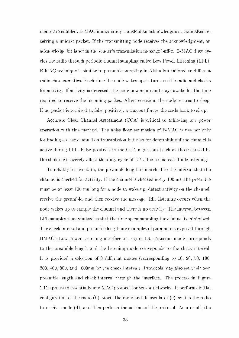
1.11 applies to essentially any MAC protocol for sensor networks. It performs initial
con�guration of the radio (b), starts the radio and its oscillator (c), switch the radio
to receive mode (d), and then perform the actions of the protocol. As a result, the
33
Figure 1.11: Current graph of a node while turning its radio on.
cost for powering up the radio is the same for all protocols. The di�erence between
protocols is how long the radio is on after it has been started and how many times
the radio is started. In this paragraph we have showed a �exible MAC protocol
that features a simple, predictable, yet scalable implementation and is tolerant to
network changes. B-MAC e�ectively performs clear channel estimation. At its
core, B-MAC exceeds the performance of other protocols though recon�guration,
feedback, and bidirectional interfaces for higher layer services. B-MAC may be
con�gured to run at extremely low duty cycles and does not force applications to
incur the overhead of synchronization and state maintenance. However B-MAC
employs an extended preamble and preamble sampling. While this �Long Power
Listening� approach is simple, asynchronous and energy-e�cient, the long preamble
introduces excess latency at each hop,is suboptimal in terms of energy consumption
and su�ers from excess energy consumption at non-target receivers. The MAC
described in the next paragraph, X-MAC [8], proposes a solutions for each of these
problems by employing shortened preamble approach that retains the advantages of
low power listening, namely low power communication, simplicity and a decoupling
of transmitter and receiver sleep schedules. X-MAC signi�cantly reduces energy
usage at both the transmitter and receiver sides, reduce per-hop latency and o�ers
additional advantages such as �exible adaptation to both bursty and periodic sensor
data sources.
34
1.3.4 X-MAC
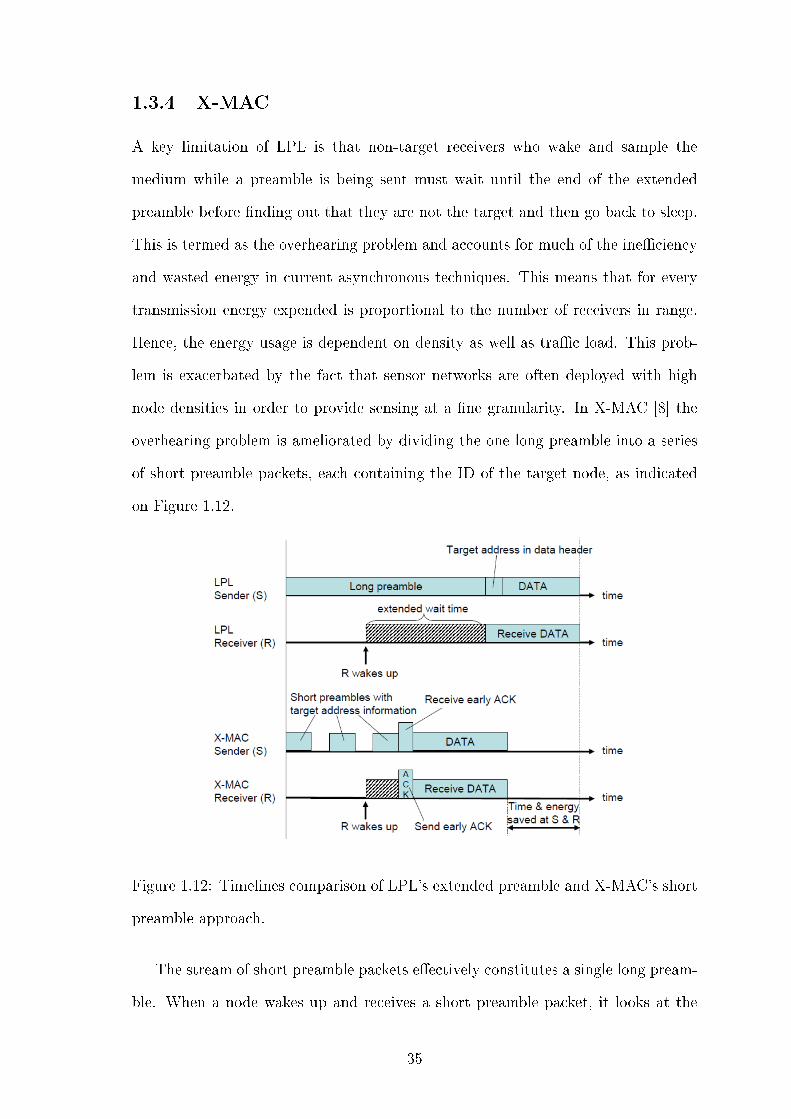
A key limitation of LPL is that non-target receivers who wake and sample the
medium while a preamble is being sent must wait until the end of the extended
preamble before �nding out that they are not the target and then go back to sleep.
This is termed as the overhearing problem and accounts for much of the ine�ciency
and wasted energy in current asynchronous techniques. This means that for every
transmission energy expended is proportional to the number of receivers in range.
Hence, the energy usage is dependent on density as well as tra�c load. This prob-
lem is exacerbated by the fact that sensor networks are often deployed with high
node densities in order to provide sensing at a �ne granularity. In X-MAC [8] the
overhearing problem is ameliorated by dividing the one long preamble into a series
of short preamble packets, each containing the ID of the target node, as indicated
on Figure 1.12.
Figure 1.12: Timelines comparison of LPL's extended preamble and X-MAC's short
preamble approach.
The stream of short preamble packets e�ectively constitutes a single long pream-
ble. When a node wakes up and receives a short preamble packet, it looks at the
35
target node identi�cation (ID) that is included in the packet. If the node is not the
intended recipient, it returns to sleep immediately and continues its duty cycling as
if the medium had been idle. If the node is the intended recipient, it remains awake
for the subsequent data packet. As seen on the Figure, a node can quickly return
to sleep, thus avoiding the overhearing problem. With this technique, the energy
consumption is independent of network density. The approach of a series of short
preamble packets scales well with increasing density, i.e. as the number of senders
increases in a neighborhood, energy expenditure remains largely �at. In comparison,
as the number of senders increase in each neighborhood of a WSN practicing LPL,
the entire WSN stays awake for increasing amounts of time.
Using an extended preamble and preamble sampling allow low power communica-
tions, yet even greater energy savings are possible if the total time spent transmitting
preambles is reduced. In traditional asynchronous techniques such as B-MAC, the
sender sends the entire preamble even though, on average, the receiver has woken up
half way through the preamble. The entire preamble needs to be sent before every
data transmission because there is no way for the sender to know that the receiver
has woken up. This is one case where more time is spent sending the preamble than
is necessary, as illustrated by the extended waiting time on Figure 1.12. Another
case occurs when there are a number of transmitters waiting to send to the some
receiver. After the �rst sender begins transmitting preamble packets, subsequent
transmitters will stay awake and wait until the channel is clear. They will then
begin sending their preamble, and this occurs for every subsequent sender. Con-
sequently, each sender transmits the entire preamble when in fact the receiver was
woken up by the �rst transmitter in the series.
In the development of X-MAC, the authors [8] have provided solutions for both
of the previous problem. Instead of sending a constant stream of preamble packets,
as would most closely approximate traditional LPL, small pauses are inert between
each packet in the series of short preamble packets, during which time the transmit-
ting node pauses to listen to the medium. These gaps enable the receiver to send an
36
early acknowledgement packet back to the sender by transmitting the acknowledge-
ment during the short pause between preamble packets. When a sender receives an
acknowledgement from the intended receiver, it stops sending preambles and sends
the data packet.
This allows the receiver to cut short the excessive preamble, which reduces per-
hop latency and energy spent unnecessarily waiting and transmitting, as can be seen
on Figure 1.12. Since the sender quickly alternates between a short preamble packet
and a short waiting time, this approach is termed strobed preamble.
In addition to shortening the preamble by use of the acknowledgement, X-MAC
also addresses the problem of multiple transmitters sending the entire preamble even
though the receiver is already awake. In X-MAC, when a transmitter is attempting
to send but detects a preamble and is waiting for a clear channel, the node listens to
the channel and if it hears an acknowledgement frame from the node that it wishes
to send to, the transmitter will back-o� a random amount and then send its data
without a preamble. The randomized back-o� is necessary since there may be more
than one transmitter waiting to send, and the random back-o� will mitigate collisions
between multiple transmitters. Also, the back-o� is long enough to allow the initial
transmitter to complete its data transmission. To enable this technique, after the
receiver receives a data packet it will remain awake for a short period of time in
case there are additional transmitters waiting to send. The period during receiver
remains awake after receiving a data packet is equal to the maximum duration of
the senders back-o� period, to assure that the receiver remains awake long enough
to receive any additional transmitters data packet.
Together, these two techniques greatly reduce excessive preambles, result in the
reduction of wasted energy, and allow for lower latency and higher throughput. In
addition, both of these techniques are broadly applicable across all forms of digital
radios, including packetized and bit stream, because the short time gaps, early
acknowledgements, and random back-o� can all be implemented in software.
37
Chapter 2
Mobility Models Design
The mobility model is designed to describe the movement pattern of mobile users,
and how their localization, velocity and acceleration change over time. Accurate
mobility modeling is necessary to mimic the behavior of mobile nodes (MNs) with
the aim of evaluate the performance of a network. Since mobility patterns may play
a signi�cant role in determining network performance, it is desirable for mobility
models to emulate the movements to targeted real life applications in a reasonable
way. When evaluating of WSNs protocols for network and MAC layers it is necessary
to choose e�ective underlying mobility models. For example, it is not appropriate
to evaluate one applications where a nodes tend to move together with Random
Waypoint Mobility Model that does not emulate moving groups. Similarly there are
some scenarios where it is not appropriate evaluate a WSN protocol with a more
realistic mobility model. Currently the di�erent mobility models are classi�ed ac-
cording several approaches [12] [13]; for all classi�cation we can point out two types
of mobility models used in the simulation of networks that we will call �ideal� and
�lifelike� models. �Lifelike� are those mobility patterns that are observed in real
life systems. A �lifelike� model provides accurate information, especially when large
number of participants are involved and the observation period is long. For simu-
lating all these scenarios that can are not be easily modeled is necessary to use an
other class of models called �ideal�. �Ideal� models attempt to realistically represent
38
the behaviors of mobility nodes (MNs) without the use of real device trace. In this
chapter with regard to �ideal� mobility model we pay more attention to mobility
model like Random Waypoint ad Gauss-Markov models. In �lifelike� paragraph,
once introduced the most important study in �lifelike� mobility models, we will de-
scribe our lifelike models that we implemented using the Mobility Framework for
OMNeT++. We will compare the approaches to mobility design, his objective and
the results extract from OMNeT++ mobility simulation.
2.1 Ideal Mobility Models
Ideal mobility models are based on simple assumptions regarding the movement
behavior of users. There are mobility models that we can use in di�erent kinds of
simulations and analytical studies of wireless sensor network. There is also a variety
of approaches for classify models for example C.Bettstetter [12] gives an overview
and classi�cation of mobility models used for simulation-based studies. We can see
on Figure 2.1 a concept map illustrating some criteria which can be used for its
classi�cation.
On the Figure 2.1 once set a mobile node behavior we can associate it a mobility
model through a sequence of question. The �rstly sequence of question allows to
couple with one of three general approaches: deterministic, hybrid or random. In
�ne the features like application, dimension and level of details characterize the level
of randomness so the complete description of mobility model under consideration.
Alternatively to the use of the concept map, recent researches have been based on
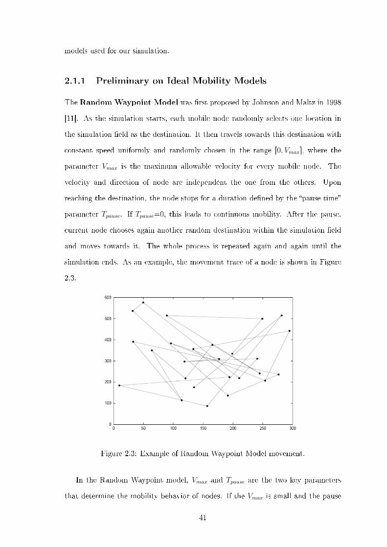
the identi�cation of models by the use of new mobility characteristics [13]. The
article points out that in the mobility models the movement of a node is more or
less restricted by its history, by other nodes in the neighborhood by the environment.
So begin it provides a categorization for various mobility models into several classes
based on their speci�c mobility characteristics so showed on Figure 2.2.
In some mobility models current movement of a mobile node is likely to be a�ected
39
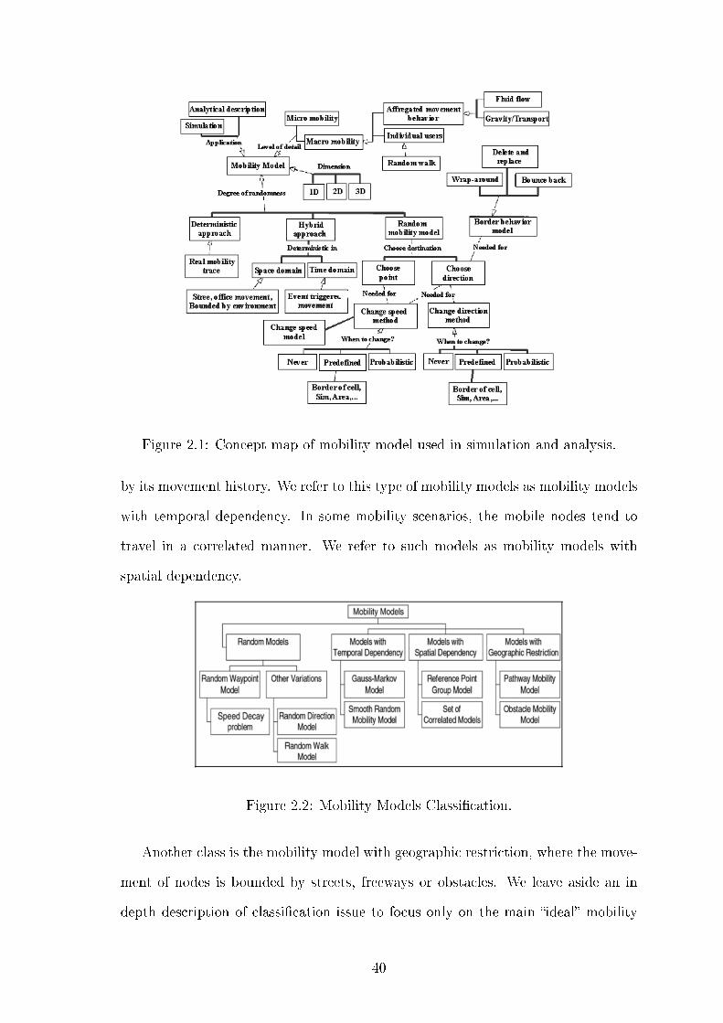
Figure 2.1: Concept map of mobility model used in simulation and analysis.
by its movement history. We refer to this type of mobility models as mobility models
with temporal dependency. In some mobility scenarios, the mobile nodes tend to
travel in a correlated manner. We refer to such models as mobility models with
spatial dependency.
Figure 2.2: Mobility Models Classi�cation.
Another class is the mobility model with geographic restriction, where the move-
ment of nodes is bounded by streets, freeways or obstacles. We leave aside an in
depth description of classi�cation issue to focus only on the main �ideal� mobility
40
models used for our simulation.
2.1.1 Preliminary on Ideal Mobility Models
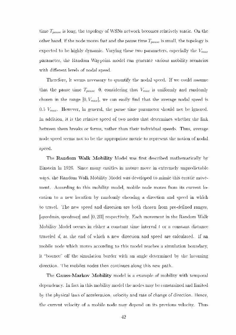
The Random Waypoint Model was �rst proposed by Johnson and Maltz in 1998
[11]. As the simulation starts, each mobile node randomly selects one location in
the simulation �eld as the destination. It then travels towards this destination with
constant speed uniformly and randomly chosen in the range [0, Vmax], where the
parameter Vmax is the maximum allowable velocity for every mobile node. The
velocity and direction of node are independent the one from the others. Upon
reaching the destination, the node stops for a duration de�ned by the �pause time�
parameter Tpause. If Tpause=0, this leads to continuous mobility. After the pause,
current node chooses again another random destination within the simulation �eld
and moves towards it. The whole process is repeated again and again until the
simulation ends. As an example, the movement trace of a node is shown in Figure
2.3.
Figure 2.3: Example of Random Waypoint Model movement.
In the Random Waypoint model, Vmax and Tpause are the two key parameters
that determine the mobility behavior of nodes. If the Vmax is small and the pause
41
time Tpause is long, the topology of WSNs network becomes relatively static. On the
other hand, if the node moves fast and the pause time Tpause is small, the topology is
expected to be highly dynamic. Varying these two parameters, especially the Vmax
parameter, the Random Waypoint model can generate various mobility scenarios
with di�erent levels of nodal speed.
Therefore, it seems necessary to quantify the nodal speed. If we could assume
that the pause time Tpause=0, considering that Vmax is uniformly and randomly
chosen in the range [0, Vmax], we can easily �nd that the average nodal speed is
0.5 Vmax. However, in general, the pause time parameter should not be ignored.
In addition, it is the relative speed of two nodes that determines whether the link
between them breaks or forms, rather than their individual speeds. Thus, average
node speed seems not to be the appropriate metric to represent the notion of nodal
speed.
The Random Walk Mobility Model was �rst described mathematically by
Einstein in 1926. Since many entities in nature move in extremely unpredictable
ways, the Random Walk Mobility Model was developed to mimic this erratic move-
ment. According to this mobility model, mobile node moves from its current lo-
cation to a new location by randomly choosing a direction and speed in which
to travel. The new speed and direction are both chosen from pre-de�ned ranges,
[speedmin, speedmax] and [0, 2Π] respectively. Each movement in the Random Walk
Mobility Model occurs in either a constant time interval t or a constant distance
traveled d, at the end of which a new direction and speed are calculated. If an
mobile node which moves according to this model reaches a simulation boundary,
it �bounce� o� the simulation border with an angle determined by the incoming
direction. The mobiles nodes then continues along this new path.
The Gauss-Markov Mobility model is a example of mobility with temporal
dependency. In fact in this mobility model the nodes may be constrained and limited
by the physical laws of acceleration, velocity and rate of change of direction. Hence,
the current velocity of a mobile node may depend on its previous velocity. Thus
42
the velocities of single node at di�erent time slots are �correlated�. We call this
mobility characteristic the Temporal Dependency of velocity. The Gauss-Markov
Mobility Model was �rst introduced by Liang and Haas [14]. In this model, the
velocity of mobile node is assumed to be correlated over time and modeled as a
Gauss-Markov stochastic process. In a two-dimensional simulation �eld, the Gauss-
Markov stochastic process can be represented by the following equations:
Vt = α ◦ Vt−1 + (1− α) ◦ υ + σ ◦√1− α2 ◦Wt−1 (2.1)
where Vt = [vxt , vyt ]
T and Vt−1 = [vxt−1, vyt−1]
T are the velocity vector at time t and
time t-1, respectively. Wt−1 = [wxt−1, w
yt−1]
T is the uncorrelated random Gaussian
process with mean 0 and variance σ2, α = [αx, αy]T , υ = [υx, υy]T , σ = [σx, σy]T
are the vectors that represent the memory level, asymptotic mean and asymptotic
standard deviation, respectively. For the sake of simplicity, we may write the general
form Equation 2.1 in a two-dimensional �eld as follows:
vxt = αvxt−1 + (1− α)υx + σx
√1− α2wx
t−1
vyt = αvyt−1 + (1− α)υy + σy√1− α2wy
t−1
When the node is going to travel beyond the boundaries of the simulation �eld,
the direction of movement is forced to �ip 180 degrees. This way, the nodes remain
away from the boundary of simulation �eld. Based on these equations, we observe
that the velocity Vt = [vxt , vyt ]
T of mobile node at time slot t is dependent on the
velocity Vt−1 = [vxt−1, vyt−1]
T at time slot t-1. Therefore, the Gauss-Markov model
is a temporally dependent mobility model whereas the degree of dependency is
determined by the memory level parameter α. α is a parameter that re�ects the
randomness of the Gauss-Markov process. By tuning this parameter we can derive
di�erent kinds of mobility behaviors in various scenarios:
43
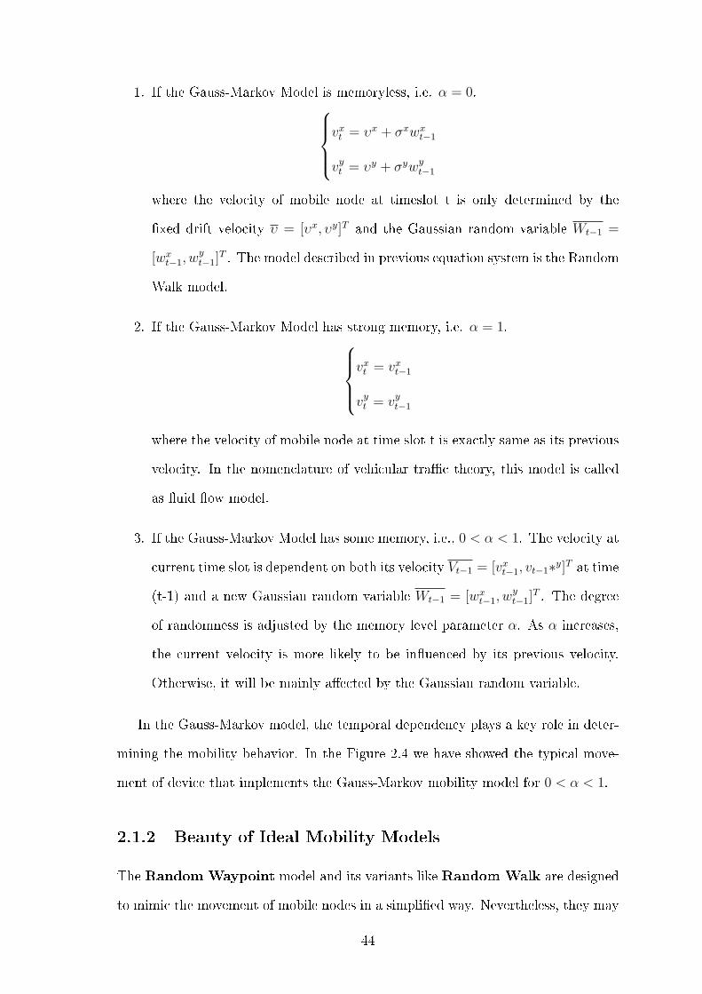
1. If the Gauss-Markov Model is memoryless, i.e. α = 0.vxt = υx + σxwx
t−1
vyt = υy + σywyt−1
where the velocity of mobile node at timeslot t is only determined by the
�xed drift velocity υ = [υx, υy]T and the Gaussian random variable Wt−1 =
[wxt−1, w
yt−1]
T . The model described in previous equation system is the Random
Walk model.
2. If the Gauss-Markov Model has strong memory, i.e. α = 1.vxt = vxt−1
vyt = vyt−1
where the velocity of mobile node at time slot t is exactly same as its previous
velocity. In the nomenclature of vehicular tra�c theory, this model is called
as �uid �ow model.
3. If the Gauss-Markov Model has some memory, i.e., 0 < α < 1. The velocity at
current time slot is dependent on both its velocity Vt−1 = [vxt−1, vt−1∗y]T at time
(t-1) and a new Gaussian random variable Wt−1 = [wxt−1, w
yt−1]
T . The degree
of randomness is adjusted by the memory level parameter α. As α increases,
the current velocity is more likely to be in�uenced by its previous velocity.
Otherwise, it will be mainly a�ected by the Gaussian random variable.
In the Gauss-Markov model, the temporal dependency plays a key role in deter-
mining the mobility behavior. In the Figure 2.4 we have showed the typical move-
ment of device that implements the Gauss-Markov mobility model for 0 < α < 1.
2.1.2 Beauty of Ideal Mobility Models
The Random Waypoint model and its variants like Random Walk are designed
to mimic the movement of mobile nodes in a simpli�ed way. Nevertheless, they may
44
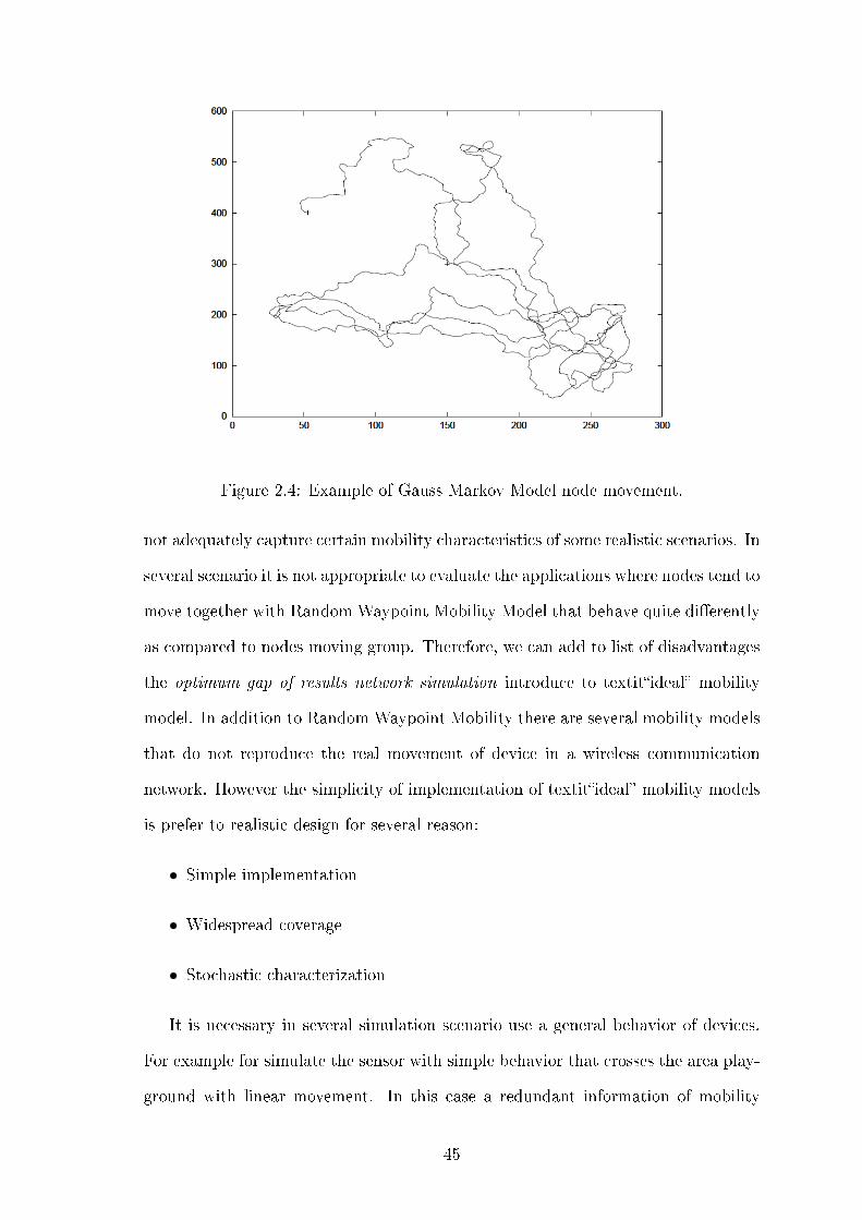
Figure 2.4: Example of Gauss Markov Model node movement.
not adequately capture certain mobility characteristics of some realistic scenarios. In
several scenario it is not appropriate to evaluate the applications where nodes tend to
move together with Random Waypoint Mobility Model that behave quite di�erently
as compared to nodes moving group. Therefore, we can add to list of disadvantages
the optimum gap of results network simulation introduce to textit�ideal� mobility
model. In addition to Random Waypoint Mobility there are several mobility models
that do not reproduce the real movement of device in a wireless communication
network. However the simplicity of implementation of textit�ideal� mobility models
is prefer to realistic design for several reason:
• Simple implementation
• Widespread coverage
• Stochastic characterization
It is necessary in several simulation scenario use a general behavior of devices.
For example for simulate the sensor with simple behavior that crosses the area play-
ground with linear movement. In this case a redundant information of mobility
45
nodes should not give a proportional vantage on performance. Moreover several
researches working on �ideal� mobility models for draw advantages from design ex-
isting. In 2004 C. Bettstetter, H. Hartenstein present in [30] a new framework for
analyzing random waypoint like models and show how the framework can be used
for providing accurate simulations of the steady state behavior. The new random
waypoint model as a renewal process and derive an accurate characterization of the
steady-state distributions of speed and residual distance, given arbitrary distribu-
tions for speed and distance of individual node movements. By the way we can
remark that the simplicity and spreading are the key of �ideal� mobility models.
2.2 Lifelike Mobility Models
Once analyzed the results obtained with our simulator for �ideal� mobility model
another object of our work is to underline the di�erences with �lifelike� by simula-
tion results. Since the mobility of the nodes directly impacts the performance of the
protocols, we want to compare the quality of simulation results obtained between
�ideal� and �lifelike� mobility models and the degree within the model chosen may
not correctly re�ect the true performance of the protocols. For this reason in the
following paragraph we will we make a general analysis of this approach's advan-
tages. Then we will describe our �lifelike� mobility models implemented on MF of
OMNeT++ and in the end results obtained by comparison with �ideal� MM.
2.2.1 Beauty of LifeLike Mobility Models
There is another approach to design a mobility model, this method make the features
of model considering the mobility of a particular typology of devices. With lifelike
approach the mobility models reproduced appear to be more realistic if compared
with �ideal� mobility models. The nature of wireless sensors network, in general for
all wireless network, have to take into account facet like multi-path, fading, and
obstacles. Moreover the solution at these issue are stressed to mobility of node. For
46
this reason it is necessary to choose a simulator that implements the mobility model
with an e�ective degree of accuracy. Since, as all said in previous paragraphs, it is
clear the trade-o�s between the �ideal� and �lifelike� mobility models. Whereas on
one hand we have simplicity and widespread features, on the other hand we have
better simulations results but more work to implement our models. It is less clear
the degree of improvement results and the threshold need to reach real simulations
results. With following we will analyze this aspect.
2.2.2 Two User Cases: Climber Mobility Model and Tracking
Down Mobility Model
The �rst Mobility Model (MM) that we have implemented is called Climber Mobility.
This �lifelike� mobility model implements a real movement of a group of climbers.
The Climber MM is thought for a wireless sensor network where a sensor monitors
the health state of the group, environment conditions or the climbers' gear, in order
to help components of the group to take a decision in danger situations. Without
considering any possible applications, next we continue the description of models.
As the Figure 2.5 shows, in this scenario we have considered �ve climbers.
In this scenario, climbers move on 2D wall. To simulate the e�ects of the third
dimension on the Line Of Sight (LOS) between two climbers, each link can be set
�on� or �o��. The �rst climber is called leader and, just like in a real situation, he
chooses the next destination point on the basis of two parameters:
• Level of Inclination tract
• Angle of progression
When the destination point has been �xed, the leader reaches it taking a time
that depends by the following parameters:
list:
• Height
47
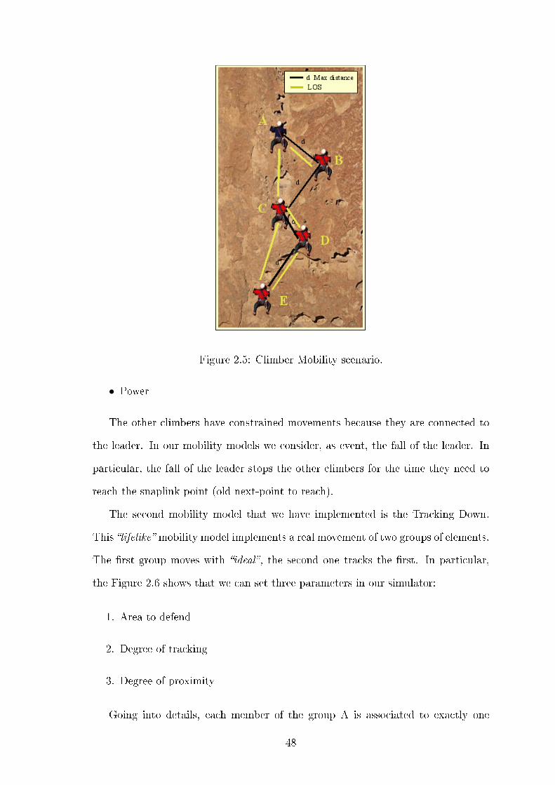
Figure 2.5: Climber Mobility scenario.
• Power
The other climbers have constrained movements because they are connected to
the leader. In our mobility models we consider, as event, the fall of the leader. In
particular, the fall of the leader stops the other climbers for the time they need to
reach the snaplink point (old next-point to reach).
The second mobility model that we have implemented is the Tracking Down.
This �lifelike� mobility model implements a real movement of two groups of elements.
The �rst group moves with �ideal�, the second one tracks the �rst. In particular,
the Figure 2.6 shows that we can set three parameters in our simulator:
1. Area to defend
2. Degree of tracking
3. Degree of proximity
Going into details, each member of the group A is associated to exactly one
48
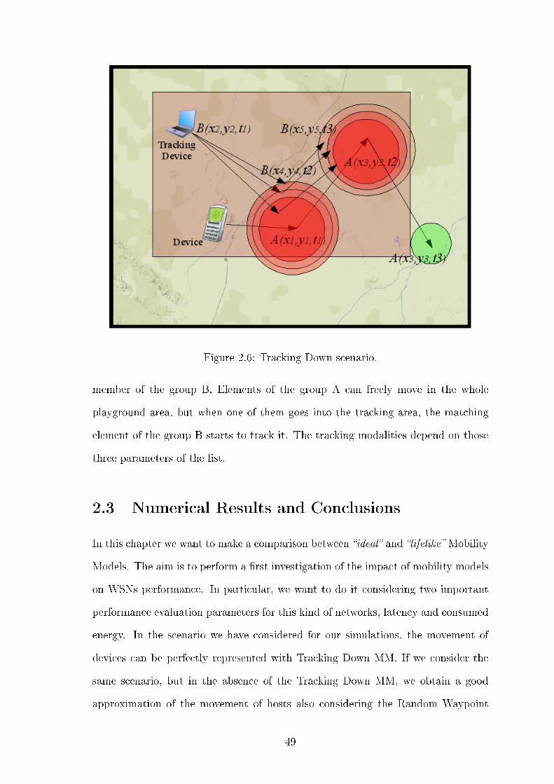
Figure 2.6: Tracking Down scenario.
member of the group B. Elements of the group A can freely move in the whole
playground area, but when one of them goes into the tracking area, the matching
element of the group B starts to track it. The tracking modalities depend on those
three parameters of the list.
2.3 Numerical Results and Conclusions
In this chapter we want to make a comparison between �ideal� and �lifelike� Mobility
Models. The aim is to perform a �rst investigation of the impact of mobility models
on WSNs performance. In particular, we want to do it considering two important
performance evaluation parameters for this kind of networks, latency and consumed
energy. In the scenario we have considered for our simulations, the movement of
devices can be perfectly represented with Tracking Down MM. If we consider the
same scenario, but in the absence of the Tracking Down MM, we obtain a good
approximation of the movement of hosts also considering the Random Waypoint
49
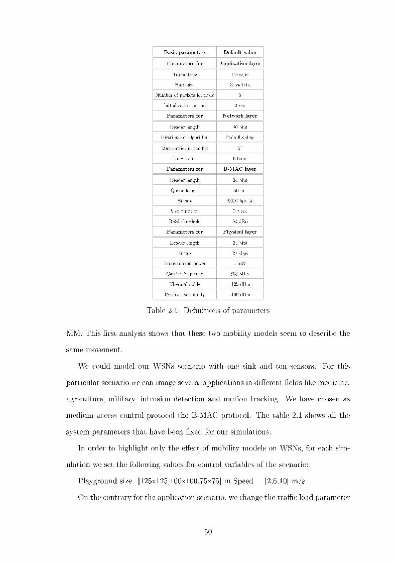
Basic parameters Default value
Parameters for Application layer
Tra�c type Periodic
Burstsize 3 packets
Number of packets for node 5
Initialization period 2 sec
Parameters for Network layer
Header length 56 bits
Distribution algorithm Plain �ooding
Max entries in the list 30
Time to live 5 hops
Parameters for B-MAC layer
Header length 24 bits
Queue length 50 bit
Bitrate 19200 bps bit
Slot duration 0.2 sec
RSSI threshold -90 dBm
Parameters for Physical layer
Header length 24 bits
Bitrate 19 kbps
Transmission power 1 mW
Carrier frequency 868 MHz
Thermal noide -125 dBm
Receiver sensibility -109 dBm
Table 2.1: De�nitions of parameters
MM. This �rst analysis shows that these two mobility models seem to describe the
same movement.
We could model our WSNs scenario with one sink and ten sensors. For this
particular scenario we can image several applications in di�erent �elds like medicine,
agriculture, military, intrusion detection and motion tracking. We have chosen as
medium access control protocol the B-MAC protocol. The table 2.1 shows all the
system parameters that have been �xed for our simulations.
In order to highlight only the e�ect of mobility models on WSNs, for each sim-
ulation we set the following values for control variables of the scenario:
Playground size=[125x125,100x100,75x75] m Speed = [2,6,10] m/s
On the contrary for the application scenario, we change the tra�c load parameter
50
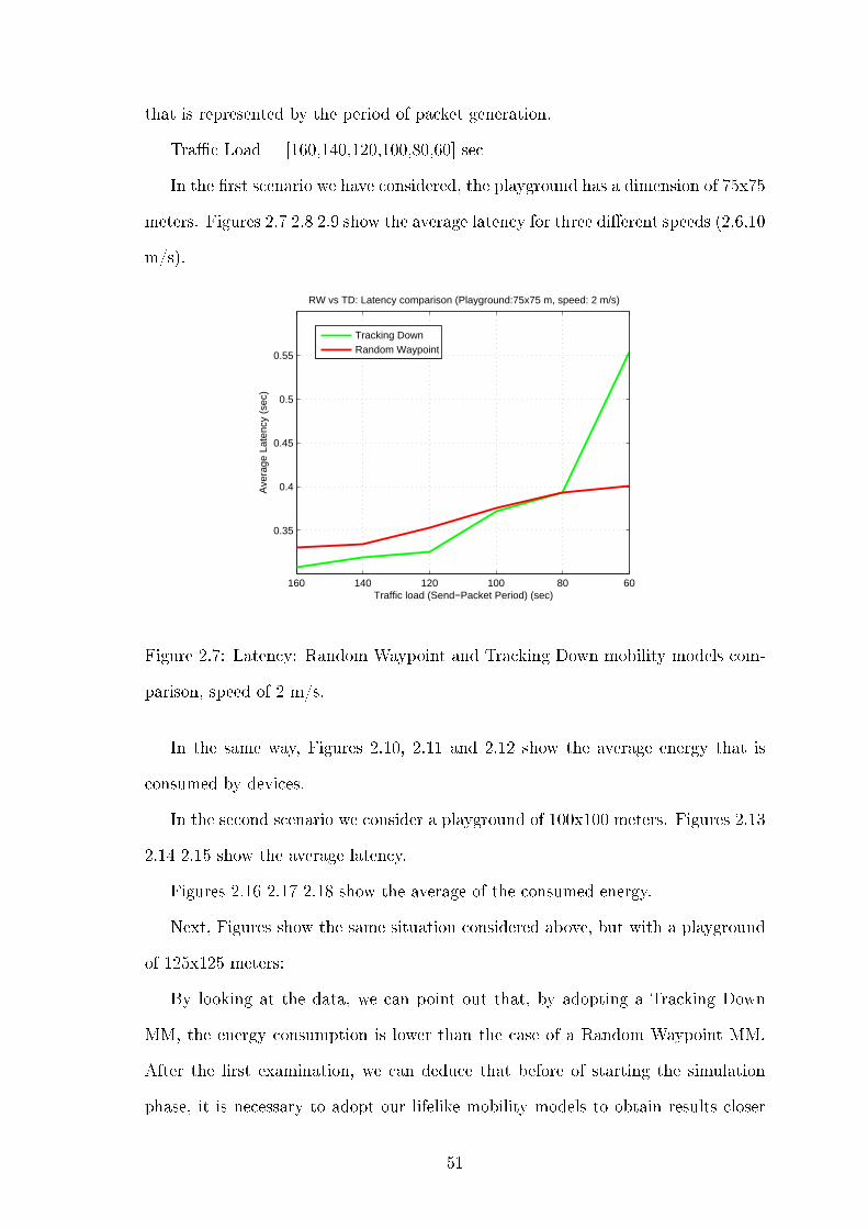
that is represented by the period of packet generation.
Tra�c Load = [160,140,120,100,80,60] sec
In the �rst scenario we have considered, the playground has a dimension of 75x75
meters. Figures 2.7 2.8 2.9 show the average latency for three di�erent speeds (2,6,10
m/s).
6080100120140160
0.35
0.4
0.45
0.5
0.55
Traffic load (Send−Packet Period) (sec)
Ave
rage
Lat
ency
(se
c)
RW vs TD: Latency comparison (Playground:75x75 m, speed: 2 m/s)
Tracking DownRandom Waypoint
Figure 2.7: Latency: Random Waypoint and Tracking Down mobility models com-
parison, speed of 2 m/s.
In the same way, Figures 2.10, 2.11 and 2.12 show the average energy that is
consumed by devices.
In the second scenario we consider a playground of 100x100 meters. Figures 2.13
2.14 2.15 show the average latency.
Figures 2.16 2.17 2.18 show the average of the consumed energy.
Next, Figures show the same situation considered above, but with a playground
of 125x125 meters:
By looking at the data, we can point out that, by adopting a Tracking Down
MM, the energy consumption is lower than the case of a Random Waypoint MM.
After the �rst examination, we can deduce that before of starting the simulation
phase, it is necessary to adopt our lifelike mobility models to obtain results closer
51
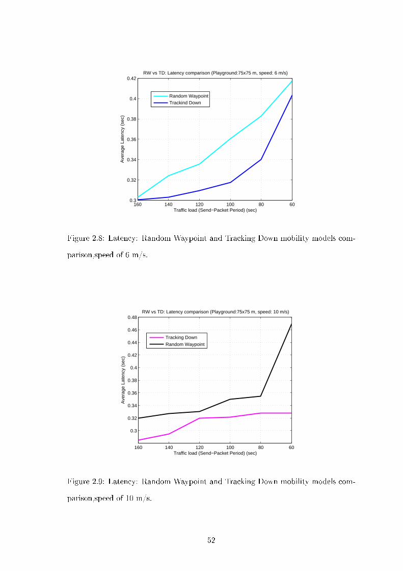
60801001201401600.3
0.32
0.34
0.36
0.38
0.4
0.42
Traffic load (Send−Packet Period) (sec)
Ave
rage
Lat
ency
(se
c)
RW vs TD: Latency comparison (Playground:75x75 m, speed: 6 m/s)
Random WaypointTrackind Down
Figure 2.8: Latency: Random Waypoint and Tracking Down mobility models com-
parison,speed of 6 m/s.
6080100120140160
0.3
0.32
0.34
0.36
0.38
0.4
0.42
0.44
0.46
0.48
Traffic load (Send−Packet Period) (sec)
Ave
rage
Lat
ency
(se
c)
RW vs TD: Latency comparison (Playground:75x75 m, speed: 10 m/s)
Tracking Down
Random Waypoint
Figure 2.9: Latency: Random Waypoint and Tracking Down mobility models com-
parison,speed of 10 m/s.
52
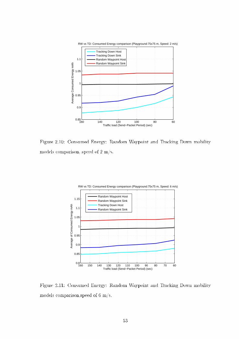
60801001201401600.85
0.9
0.95
1
1.05
1.1
Traffic load (Send−Packet Period) (sec)
Ave
rage
Con
sum
ed E
nerg
y m
Ah
RW vs TD: Consumed Energy comparison (Playground:75x75 m, Speed: 2 m/s)
Tracking Down HostTracking Down SinkRandom Waypoint HostRandom Waypoint Sink
Figure 2.10: Consumed Energy: Random Waypoint and Tracking Down mobility
models comparison, speed of 2 m/s.
607080901001101201301401501600.8
0.85
0.9
0.95
1
1.05
1.1
1.15
Traffic load (Send−Packet Period) (sec)
Ave
rage
of C
onsu
med
Ene
rgy
mA
h
RW vs TD: Consumed Energy comparison (Playground:75x75 m, Speed: 6 m/s)
Random Waypoint Host
Random Waypoint Sink
Tracking Down Host
Random Waypoint Sink
Figure 2.11: Consumed Energy: Random Waypoint and Tracking Down mobility
models comparison,speed of 6 m/s.
53
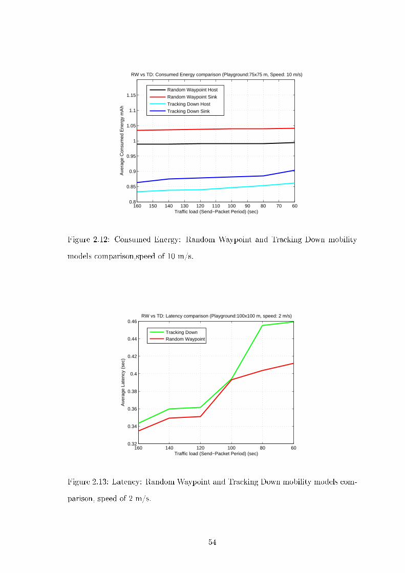
607080901001101201301401501600.8
0.85
0.9
0.95
1
1.05
1.1
1.15
Traffic load (Send−Packet Period) (sec)
Ave
rage
Con
sum
ed E
nerg
y m
Ah
RW vs TD: Consumed Energy comparison (Playground:75x75 m, Speed: 10 m/s)
Random Waypoint Host
Random Waypoint Sink
Tracking Down Host
Tracking Down Sink
Figure 2.12: Consumed Energy: Random Waypoint and Tracking Down mobility
models comparison,speed of 10 m/s.
60801001201401600.32
0.34
0.36
0.38
0.4
0.42
0.44
0.46
Traffic load (Send−Packet Period) (sec)
Ave
rage
Lat
ency
(se
c)
RW vs TD: Latency comparison (Playground:100x100 m, speed: 2 m/s)
Tracking DownRandom Waypoint
Figure 2.13: Latency: Random Waypoint and Tracking Down mobility models com-
parison, speed of 2 m/s.
54
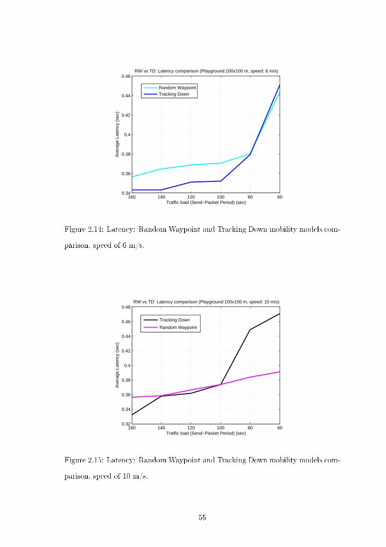
60801001201401600.34
0.36
0.38
0.4
0.42
0.44
0.46
Traffic load (Send−Packet Period) (sec)
Ave
rage
Lat
ency
(se
c)
RW vs TD: Latency comparison (Playground:100x100 m, speed: 6 m/s)
Random WaypointTracking Down
Figure 2.14: Latency: Random Waypoint and Tracking Down mobility models com-
parison, speed of 6 m/s.
60801001201401600.32
0.34
0.36
0.38
0.4
0.42
0.44
0.46
0.48
Traffic load (Send−Packet Period) (sec)
Ave
rage
Lat
ency
(se
c)
RW vs TD: Latency comparison (Playground:100x100 m, speed: 10 m/s)
Tracking Down
Random Waypoint
Figure 2.15: Latency: Random Waypoint and Tracking Down mobility models com-
parison, speed of 10 m/s.
55

60801001201401600.85
0.9
0.95
1
1.05
1.1
Traffic load (Send−Packet Period) (sec)
Ave
rage
Con
sum
ed E
nerg
y m
Ah
RW vs TD: Consumed Energy comparison (Playground:100x100 m, Speed: 2 m/s)
Random Waypoint Host
Random Waypoint Sink
Tracking Down Host
Tracking Down Sink
Figure 2.16: Latency: Random Waypoint and Tracking Down mobility models com-
parison, speed of 2 m/s.
60708090100110120130140150160
0.85
0.9
0.95
1
1.05
1.1
Traffic load (Send−Packet Period) (sec)
Ave
rage
Con
sum
ed E
nerg
y m
Ah
RW vs TD: Consumed Energy comparison (Playground:100x100 m, Speed: 6 m/s)
Random Waypoint Host
Random Waypoint Sink
Tracking Down Host
Tracking Down Sink
Figure 2.17: Latency: Random Waypoint and Tracking Down mobility models com-
parison,speed of 6 m/s.
56
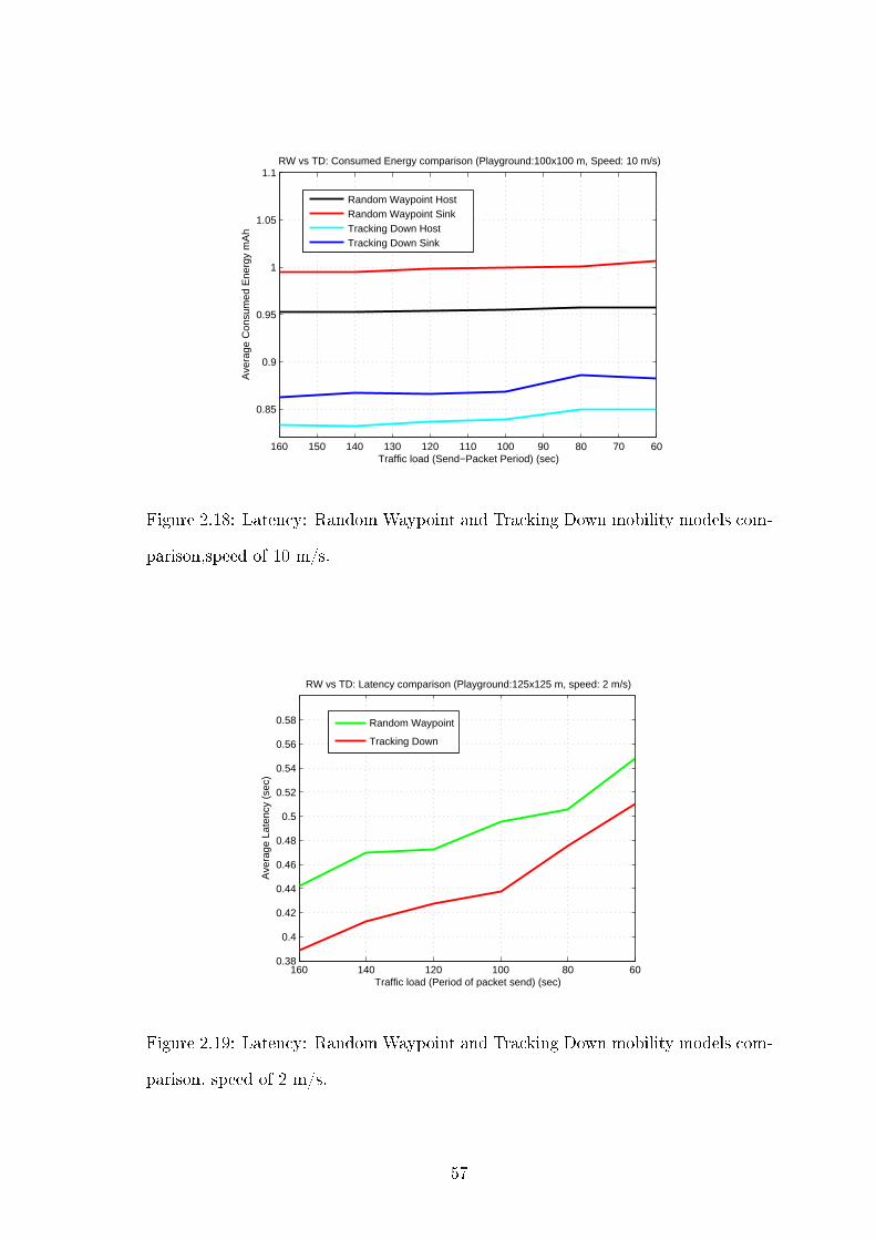
60708090100110120130140150160
0.85
0.9
0.95
1
1.05
1.1
Traffic load (Send−Packet Period) (sec)
Ave
rage
Con
sum
ed E
nerg
y m
Ah
RW vs TD: Consumed Energy comparison (Playground:100x100 m, Speed: 10 m/s)
Random Waypoint HostRandom Waypoint SinkTracking Down HostTracking Down Sink
Figure 2.18: Latency: Random Waypoint and Tracking Down mobility models com-
parison,speed of 10 m/s.
60801001201401600.38
0.4
0.42
0.44
0.46
0.48
0.5
0.52
0.54
0.56
0.58
Traffic load (Period of packet send) (sec)
Ave
rage
Lat
ency
(se
c)
RW vs TD: Latency comparison (Playground:125x125 m, speed: 2 m/s)
Random Waypoint
Tracking Down
Figure 2.19: Latency: Random Waypoint and Tracking Down mobility models com-
parison, speed of 2 m/s.
57
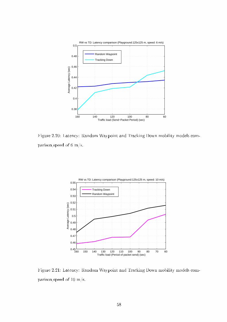
6080100120140160
0.38
0.4
0.42
0.44
0.46
0.48
0.5
Traffic load (Send−Packet Period) (sec)
Ave
rage
Lat
ency
(se
c)
RW vs TD: Latency comparison (Playground:125x125 m, speed: 6 m/s)
Random Waypoint
Tracking Down
Figure 2.20: Latency: Random Waypoint and Tracking Down mobility models com-
parison,speed of 6 m/s.
607080901001101201301401501600.45
0.46
0.47
0.48
0.49
0.5
0.51
0.52
0.53
0.54
0.55
Traffic load (Period of packet send) (sec)
Ave
rage
Lat
ency
(se
c)
RW vs TD: Latency comparison (Playground:125x125 m, speed: 10 m/s)
Tracking Down
Random Waypoint
Figure 2.21: Latency: Random Waypoint and Tracking Down mobility models com-
parison,speed of 10 m/s.
58
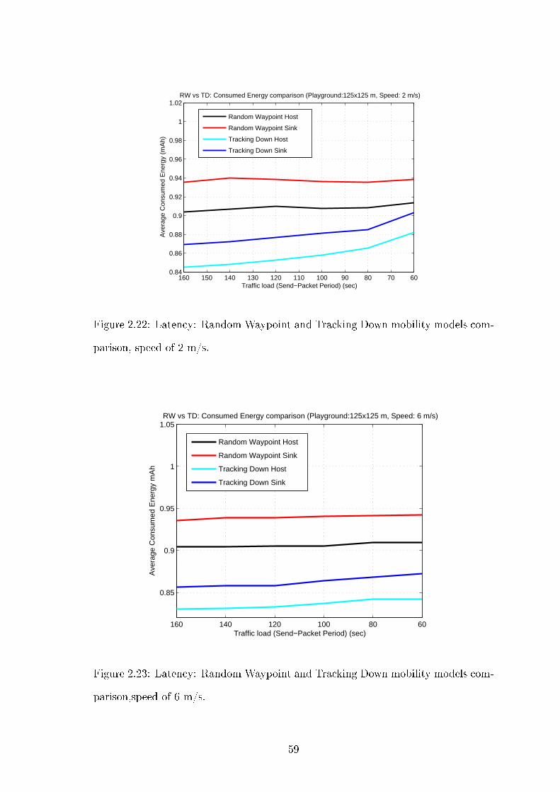
607080901001101201301401501600.84
0.86
0.88
0.9
0.92
0.94
0.96
0.98
1
1.02
Traffic load (Send−Packet Period) (sec)
Ave
rage
Con
sum
ed E
nerg
y (m
Ah)
RW vs TD: Consumed Energy comparison (Playground:125x125 m, Speed: 2 m/s)
Random Waypoint Host
Random Waypoint Sink
Tracking Down Host
Tracking Down Sink
Figure 2.22: Latency: Random Waypoint and Tracking Down mobility models com-
parison, speed of 2 m/s.
6080100120140160
0.85
0.9
0.95
1
1.05
Traffic load (Send−Packet Period) (sec)
Ave
rage
Con
sum
ed E
nerg
y m
Ah
RW vs TD: Consumed Energy comparison (Playground:125x125 m, Speed: 6 m/s)
Random Waypoint Host
Random Waypoint Sink
Tracking Down Host
Tracking Down Sink
Figure 2.23: Latency: Random Waypoint and Tracking Down mobility models com-
parison,speed of 6 m/s.
59
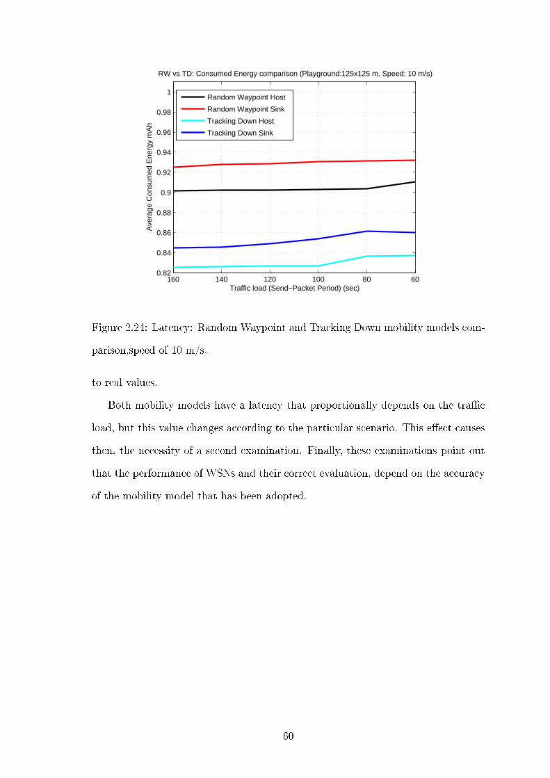
60801001201401600.82
0.84
0.86
0.88
0.9
0.92
0.94
0.96
0.98
1
Traffic load (Send−Packet Period) (sec)
Ave
rage
Con
sum
ed E
nerg
y m
Ah
RW vs TD: Consumed Energy comparison (Playground:125x125 m, Speed: 10 m/s)
Random Waypoint Host
Random Waypoint Sink
Tracking Down Host
Tracking Down Sink
Figure 2.24: Latency: Random Waypoint and Tracking Down mobility models com-
parison,speed of 10 m/s.
to real values.
Both mobility models have a latency that proportionally depends on the tra�c
load, but this value changes according to the particular scenario. This e�ect causes
then, the necessity of a second examination. Finally, these examinations point out
that the performance of WSNs and their correct evaluation, depend on the accuracy
of the mobility model that has been adopted.
60
Chapter 3
Characterizing Mobility Models
Designs of algorithms and protocols for WSN generally assume individual sensor
nodes to be static. However, some recent applications of WSN (e.g. in medical
care and disaster response) make use of mobile sensor nodes. Moreover, WSNs
mobile devices have limited power and computing capacity. Therefore, mobility is
also expected to a�ect networks performance signi�cantly. For example, in high
mobility scenarios frequent changes of topology, caused by node movement, may
result in disruption of established routes, leading to packet losses and that decreases
capacity due to increase of network latency. Several past studies have explored
mobility issues and impact of mobility models in network performance. Thus, in
order to design a protocol or an algorithm from WSNs it is essential to evaluate the
impact of mobility on system performances. The characterization of such mobility
models characteristic is still an open challenge. The �rst aim of this chapter is
investigate how mobility models of wireless sensor can be e�ciently characterized.
The second aim is de�ne the set of best parameters (metrics) needed to di�erentiate
mobility models. To that end in 2003, F. Bai and N. Sadagopan [27] and [28],
have de�ned mobility metrics of several mobility models, in order to identify a set of
relationship between network performance and mobility models. In particular in [27]
and [28] the authors studied the impact of mobility models on protocol performances
considering the following mobility models characteristics:
61
• Spatial dependence of movement among nodes
• Temporal dependence of movement of a node over time
• Obstacles
In [30] C. Bettstetter and H. Hartenstein give a formal description of Random
Waypoint Mobility Model (RWP) [10] in terms of a discrete-time stochastic process.
They investigate some of its fundamental stochastic properties with respect to:
• Transition length and time of a mobile node between two waypoints
• Spatial distribution of nodes
• Direction angle at the beginning of a movement transition
• Cell changing rate
Results of [30] are the practical value for performance analysis of mobile net-
works and deeper understanding of behavior of Random Waypoint mobility model.
Although e�ects of mobility models on networks performance are not the aim of
this chapter, the characterization of mobility models parameters showed in [27],
[28], [29] and [30] are a starting point of our the mobility models identi�cation al-
gorithm proposed in fourth chapter. Having said that this chapter is organized as
follows:
• In section 3.1 we present currently proposed �mobility metrics� [27], [28],
[29] in the general case of WSNs.
• In section 3.2 we provide a survey on fundamental stochastic properties of
Random Waypoint mobility model
• Eventually, in section 3.3 we critically present some mobility models imple-
mented in Mobility Framework for OMNeT++ and we compare them in terms
of average link duration for several simulation scenarios
62
3.1 Mobility Metrics
Mobility metrics attempt to achieve an extract characterization of mobility models
and connectivity between mobile nodes. These metrics are classically used to ex-
plain the impact of mobility on protocol performance [27], [28], [29]. Hereafter we
introduce some basic notation that will be used in the chapter:
1.−→Vi(t): Velocity vector of node i at time t.
2. |−→Vi(t)|: Speed of node i at time t.
3. θi(t): Angle made by−→Vi (t) at time t with the X-axis.
4. −→αi(t): Acceleration vector of node i at time t.
5. xi(t): X co-ordinate of node i at time t.
6. yi(t): Y co-ordinate of node i at time t.
7. Di,j(t): Euclidean Distance between nodes i and j at time t.
8. RD(−→a (t),−→b (t′)): Relative Direction(RD) (or cosine of the angle) between the
two vectors −→a (t),−→b (t′) is given by
−→a (t)·−→b (t′)
|−→a (t)|∗|−→b (t′)|
9. SR(−→a (t),−→b (t′)): Speed Ratio(SR) between the two vectors −→a (t),
−→b (t′) is
given by min min|−→a (t)|,|−→b (t′)|
max|−→a (t)|,|−→b (t′)|
10. R: Transmission range of a mobile node.
11. N: Number of mobile nodes.
12. T: Simulation time.
13. random(): function which returns a uniformly distributed value in the interval
[−1, 1].
63
Mobility metrics could be used to di�erentiate di�erent mobility patterns pre-
sented in literature. The basis of di�erentiation is analyze spatial dependence, tem-
poral dependence and geographic restrictions.
Degree of Spatial Dependence: It is extent of similarity of the velocities of
two nodes that are not too far apart. We can express such relation as follow:
Dspatial(i, j, t) = RD(−→vi (t),−→vj (t)) ∗ SR(−→vi (t),−→vj (t)) (3.1)
The value of Dspatial(i, j, t) is high when nodes i and j travel in more or less the
same direction and at almost similar speeds. However, Dspatial(i, j, t) decreases if
the Relative Direction or the Speed Ratio decreases. As it is unlike for a node's
motion to be spatially dependent on a far o� node, we add the condition that
Di,j(t) > c1 ∗R =⇒ Dspatial(i, j, t) = 0 (3.2)
where c1 > 0 is a constant. Average Degree of Spatial Dependence: It is the
value of Dspatial(i, j, t) averaged over node pairs and time instants satisfying certain
conditions. This can be expressed as follow:
D̄spatial =
∑Tt=1
∑Ni=1
∑Nj=i+1 Dspatial(i, t, t)
P(3.3)
where P is the number of tuples (i, j, t) such that Dspatial(i, j, t) ̸= 0. Thus,
if mobile nodes move independently of one another, then the mobility pattern is
expected to have smaller value for D̄spatial. On the other hand, if the node movement
is coordinated by a central entity, or in�uenced by nodes in its neighborhood, such
that they move in similar directions and at similar speeds, then the mobility pattern
is expected to have a higher value for D̄spatial.
Degree of Temporal Dependence: It is the extent of similarity of the veloc-
ities of a node at two time slots that are not too far apart. It is a function of the
acceleration of the mobile node and the geographic restrictions. We can express it
as follow:
64
Dtemporal(i, j, t′) = RD(−→vi (t),−→vi (t′)) ∗ SR(−→vi (t),−→vi (t′)) (3.4)
The value of Dtemporal(i, j, t′) is high when the node moves in more or less the
same direction and almost at the same speed over a certain time interval that can be
de�ned. However, Dtemporal(i, j, t′) decreases if the Relative Direction or the Speed
Ratio decreases. Arguing in a way similar to that for Dspatial(i, j, t), we have the
following condition
|t− t′| > c2 =⇒ Dtemporal(i, t, t′) = 0
where c2 > 0 is a constant. Average Degree of Temporal Dependence: It is the
value of Dtemporal(i, j, t′) averaged over nodes and time instants satisfying certain
condition. Formally,
D̄temporal =
∑Ni=1
∑Tt=1
∑Tt′=i Dtemporal(i, t, t
′)
P(3.5)
where P is the number of tuples (i, t, t') such that Dtemporal(i, t, t′) ̸= 0. Thus,
if the current velocity of a node is completely independent of its velocity at some
previous time step, then the mobility pattern is expected to have a smaller value
for D̄temporal. However, if the current velocity is strongly dependent on the velocity
at some previous time step, then the mobility pattern is expected to have a higher
value for D̄temporal. Since networks WSNs performance is a�ected by the network
topology dynamics, it is worth to considered some metrics to analyze the e�ect of
mobility on the connectivity graph between the mobile nodes.
The connectivity graph metrics aim to study this e�ect. The connectivity graph
is the graph G = (V,E), such that |V | = N and at time t, a link (i, j) ∈ E if
Di,j(t) ≤ R. Let X(i, j, t) be an indicator random variable which assumes a value 1
if there is a link between nodes i and j at time t. X(i, j) = maxTt=1X(i, j, t) be an
indicator random variable which is 1 if a link existed between nodes i and j at any
time during the simulation, 0 otherwise. Number of Link Changes: Number of
link changes for a pair of nodes i and j is the number of times the link between them
65
switches from �down� to �up�. Formally,
LC(i, j) =T∑t=1
C(i, j, t) (3.6)
where C(i,j,t) is an indicator random variable such that C(i, j, t) = 1 if X(i, j, t−
1) = 0 and X(i, j, t) = 1 i.e. if the link between nodes i and j is down at time (t−1),
but comes up at time t. Average Number of Link Changes : It is the value of LC(i,j)
averaged over node pairs satisfying some conditions. We can express relation as:
L̄C =
∑Ni=1
∑Nj=i+1 LC(i, j))
P(3.7)
where P is the number of pairs i,j such that X(i, j) ̸= 0.
Link Duration: It is the average duration of the link existing between two
nodes i and j. It is a measure of stability of the link between these nodes. Formally,
LD(i, j) =
∑T
t=1 X(i,j,t)
LCi,jif LC(i, j) ̸= 0∑T
t=1 X(i, j, t)LCi,j otherside
(3.8)
Average Link Duration: It is the value of LD(i,j) averaged over node pairs sat-
isfying certain condition.
Formally:
L̄D =
∑Ni=1
∑Nj=i+1 LD(i, j))
P(3.9)
where P is the number of pairs i,j such that X(i, j) ̸= 0.
Path Availability: It is the fraction of time during which a path is available
between two nodes i and j. The node pairs of interest are the ones that have
communication tra�c between them. Formally,
PA(i, j) =
∑T
t=starti,jA(i,j,t)
T−starti,jif T − start(i, j) > 0
0 otherside
(3.10)
66
where A(i,j t) is an indicator random variable which has a value 1 if a path is
available from node i to node j at time t, and has a value 0 otherwise. Start(i, j) is
the time when communication tra�c between nodes i and j starts.
Average Path Availability : It is the value of PA(i,j) averaged over node pairs
satisfying certain conditions. Formally,
P̄A =
∑Ni=1
∑Nj=i+1 PA(i, j))
P
where P is the number of pairs i, j such that T − start(i, j) > 0.
3.2 Stochastic Properties
Random Waypoint (RWP) model is a very popular and commonly used mobility
models. An interesting aspect is the de�nition of RWP as a discrete-time stochastic
process. C. Bettstetter, H. Hartenstein and X. Pérez-Costa, in 2004 [30], considering
speed behavior and direction change behavior, have de�ned for Random Waypoint
model the expected value, variance, and probability density function of the transi-
tion length in a rectangular system area and also the mapping from transition length
to duration, in scenarios with and without pause time at the destination waypoints.
RWP Stochastic Process: The random variable representing the Cartesian coor-
dinates of the waypoint that a node j chooses in its movement period i is denoted
by the vector P (j)i . With this de�nition, the movement trace of an RWP node j
could be formally described as a discrete-time stochastic process, given by selecting
a random waypoint P (j)i for each movement period i :
{P (j)i }i∈N0 = P
(j)0 , P
(j)1 , P
(j)2 , P
(j)3 . . . (3.11)
These waypoints are independently and identically distributed (i.i.d.) using a
uniform random distribution over the system space A. Since each node moves inde-
pendently of other nodes, it is su�cient to study the movement process of a single
node. Thus, we will thus often omit the index j. Let consider a node that randomly
67
chooses a new speed Vi for movement from P(i−1) to Pi and a pause time Tp,i at
waypoint Pi. The complete movement process of node is then given by:
{(Pi, Vi, Tp,i}i∈N = (P1, V1, Tp,1), (P2, V2, Tp,2), (P3, V3, Tp,3) . . . (3.12)
Where an additional waypoint P0 is needed for initialization. A sample of this
process is denoted by {pi, vi, τp,i}. A movement period i can be completely described
by the vector {p(i−1), pi, vi, τp,i}. When we just refer to a single random variable of a
process, we omit the index i and just write P, V , or Tp. The values for the pause time
are chosen from a bounded random distribution fTp(τp) in the interval [0, τp,max] with
τp,max < ∞ and a well-de�ned expected value E{Tp}. In general speed is also chosen
from a random distribution fV (v) within the interval [vmin, vmax] with vmin > 0 and
vmax < ∞.
Transition Length and Duration: As de�ned above, the stochastic process
representing the RWP movement of a node j is given by the sequence of random
waypoints P (j)0 , P
(j)0 , . . .. The corresponding stochastic process of distances between
two consecutive waypoints is given by:
{L(j)i }i∈N = L
(j)1 , L
(j)2 , L
(j)3 , . . . L
(j)i = ∥P (j)
i − P(j)i-1 ∥ (3.13)
A sample of this process is written as {l(j)i }. While the random waypoints are
i.i.d. per de�nition, the distances are not stochastically independent, essentially
because the endpoint of one movement period i is the starting point of the successive
movement period (i+ 1). The expected value of L can be interpreted in two ways:
E{L} = limm−→∞
1
m
m∑i=1
l(j)i︸ ︷︷ ︸
time averange of node j
= limn−→∞
1
n
n∑j=1
l(j)i︸ ︷︷ ︸
ensemble averange at period i
(3.14)
The time average of the transition lengths experienced by a single RWP node
j over a long-run simulation (m → ∞) is equal to the ensemble average of one
period i in an RWP process with many nodes (n → ∞). In the notation of random
68
processes, we thus have a mean-ergodic property of the RWP mobility model. While
this result is intuitively convincing, the proof is not trivial since the random variables
L1, L2, L3, . . . are not stochastically independent. But despite the fact that �last
endpoint equals next starting point�, the ergodic property could be seen as follows.
Assume we look at a random process given by:
{L2i−1}i∈N = L1, L3, L5 . . . (3.15)
i.e., we look on y at every second variable of the original process of random
distances. The length L1 is a deterministic function of P0 and P1, the length L3
a deterministic function of P2 and P3, and so on. Since P0, P1, P2, . . . are i.i.d.
random variables, it follows that L1, L3, . . . are also independent. The mean-ergodic
property is obtained immediately in this sub-process because both the time and
ensemble average is formed by mutually independent variables. The same is true for
the sub-process:
{L2i}i∈N = L2, L4, L6 . . . (3.16)
Now, combining these two sub-processes does not change the asymptotic be-
havior of the time averages of the combined process, thus, Equation 3.14 holds.
Similarly the distribution-ergodic property of the process can be obtained.
With respect to this problem the analysis can be simpli�ed by considering only the
distribution of the distance between two independent points placed uniformly in the
system area. In the following, there are no di�erences in notation between the �dis-
tance between two consecutive waypoints� and the �distance between two independent
random points sampled from a uniform distribution�. Both are represented by the
random variable L.
Transition Length on One-Dimensional Line Segment: Considering one-
dimensional line segment [0, a], two random points are uniformly placed on this
segment, i.e., the pdf of a point's location P = Px is:
69
fPx(x) =
1a
for 0 ≤ x ≤ a
0 else
(3.17)
Since both points are independent from each other, their joint pdf is:
fPx1Px2(x1, x2) = fPx(x1)fPx(x2) =
1a2
for 0 ≤ x1, x2 ≤ a
0 else
(3.18)
The distance between two random points is de�ned by L = |Px1 − Px2 |. The
probability that this distance is smaller than a given value l can be computed through
the integral of the joint probability density function (pdf) over the area de�ned by
D = |x1 − x2| ≤ l in the x1 − x2 − space, i.e.,
P (L ≤ l) =
∫ ∫D
fPx1Px2(x1, x2)dx2dx1 (3.19)
for 0 ≤ l ≤ a. Clearly, P (L ≤ l) = 1 for l > a. Taking into account the bounds
of both D and fPx1Px2(x1, x2), we obtain the cumulative distribution function (cdf)
P (L ≤ l) =1
a2(
∫ l
0
∫ x1+l
0
dx2dx1+
∫ a-l
l
∫ x1+l
x1−l
dx1dx2+
∫ a
a−l
∫ a
x1−l
dx1dx2) =1
a2l2+
2
al
(3.20)
The derivative of this function with respect to l yields by de�nition the desired
fL(l) =∂
∂lP (L ≤ l) =
1
a2l2 +
2
al (3.21)
for 0 ≤ l ≤ a, and fL(l) = 0 otherwise. The expected distance is
EL =
∫ a
0
lfL(l)dl =1
3a (3.22)
and its variance yields:
EL2 =
∫ a
0
l2fL(l)dl =1
6a2 (3.23)
70
With the above results on ergodicity, these stochastic properties of the distances
between a pair of independently uniformly distributed points also represent the
stochastic properties of the moved distance of an RWP node within one period. We
describe distribution of transition length L in a rectangular area of size a x b and
its expected value.
fL(l) =4l
a2b2· f0(l) (3.24)
with:
f0(l) =
π2ab− al − bl + 1
2l2 for 0 ≤ l ≤ b
ab arcsin bl+ a
√l2 − b2 − 1
2b2 − al for b < l < a
ab arcsin bl+ a
√l2 − b2 − 1
2b2−
ab arccos al+ b
√l2 − a2 − 1
2a2 − 1
2l2 fora ≤ l ≤
√a2 + b2
0 otherside
(3.25)
The expected value of L is:
E{L} =1
15[a3
b2+b3
a2+√a2 + b2(3−a2
b2− b2
a2)]+
1
6[b2
aarccosh
√a2 + b2
a+a2
barccosh
√a2 + b2
b]
(3.26)
The variance of L is given by:
E{L2} =1
6(a2 + b2) (3.27)
Transition Time: With the previous results on the transition length is possible
calculate the stochastic properties of the transition time [30], i.e., the time necessary
to node to move from one waypoint to the next waypoint. The corresponding random
variable is denoted by T and an outcome is written as τ .
If the speed of a node is constant during the entire movement process, i.e.,
Vi = υ = const ∀i and v > 0, we have:
71
T =1
υL (3.28)
Hence, the expected transition time is :
E{T} =1
υE{L} (3.29)
and its pdf can be computed by:
fT (τ) = vfL(υτ) (3.30)
with E{L} and fL taken from 3.24 3.26, respectively. It is possible to consider
the case in which the speed of a node is not constant but chosen from a random
distribution fV (υ) at each waypoint (and then stays constant during one transition).
We require vmin ≤ V ≤ vmax and vmin > 0 and can write:
T +L
V(3.31)
In this case, the random variable T is formed as a function g(L, V ) = LVof two
random variables L and V . In general, the expected value of a variable g(L,V) can
be expressed in terms of the joint pdf fLV (l, υ) as [30]:
E{g(L, V )} =
∫ ∞
∞
∫ ∞
∞g(l, υ)fLV (l, υ)dυ (3.32)
In our case, L and V are independent, and thus their joint pdf is fLV (l, υ) =
fL(l)fV (v). The expected value can then be simpli�ed to:
E{T} = E{L}∫ υ
υmin
max1
υfV (υ)dυ (3.33)
The pdf of T = LVcan be computed by:
fT (τ) =
∫ υ
υmin
maxυfL(υτ)dυ (3.34)
for 0 ≤ τ ≤ τmax with τmax = lmax
υmaxand fT (τ) = 0 otherwise.
72
3.3 Random Waypoint and Gauss-Markov mobility
metrics
Even if a stochastic characterization of mobility would be an interesting approach to
compare di�erent mobility models, up to now researches provide only the stochastic
characterization of the Random Waypoint model. This means that we need to wait
for future works to characterize mobility models through stochastic method.
Considering those mobility models implemented in the Mobility Framework for
OMNeT++ and those scenarios tested, we have performed our personal examina-
tions on graph connection metrics. In particular we have considered the Gauss-
Markov and the Random Waypoint as mobility models and the link duration among
nodes as parameter for the connections graph. A Java software has been used in
order to obtain results from the mobility models examination. This application,
called BonnMotion [26], creates and analyzes mobility scenarios and supports the
following mobility models:
• Random Waypoint
• Gauss-Markov
• Reference Point Group
• Disaster Area
• Manhattan Grid
BonnMotion could be used to reproduce devices movement in the Mobility
Framework for OMNeT++. Thanks to this software is possible to create a �le
.xml, where every link represents, point-by-point, the movement of each node in the
time. This means that there is one line for each node. Each of them contains all
the waypoints. A waypoint is the coordinate where the movement of a node (e.g.
direction, velocity) changes. Waypoint could be represented by:
73
• The simulation time (s) at which waypoint is reached by the node
• The coordinates (x,y) of the position of waypoint
Moreover, this software provides also some functionalities to analyze those .xml
�les created before. There are two di�erent approaches; the default approach cal-
culates �overall� statistics (averaged over the simulation time) while the other one
calculates �progressive� statistics (values of metrics for certain points in time). In
the default mode, the application creates a �le with the su�x �.stats� that contains
several information. In this kind of �le, each row describes those values obtained at
di�erent trasmission range, while each column describes a network parameter that
has been calculated. We have analyzed the column that corresponds to the average
link duration value that is relative to all those links that are active in the simulation
scenario.
According to WSNs features, we have tested the link duration by considering �ve
di�erent values of the transmission range among the devices. In order to achieve a
deeper examination of the whole environment, we have also changed the speed of
nodes. Therefore, for each transmission range we have measured the average link
duration for di�erent speed of nodes. In particular:
• Transmission range: [40, 60, 80, 100, 120] m
• Speed: [5, 10, 15, 20, 25, 30, 35, 40, 45, 50, 55, 60] m\s
The aim of the study is to �nd out possible di�erences among average of link
duration value of mobility models under exams. These exams will model the pro-
posed �Guess-Who� algorithm (see section 4) that we will describe in the following
chapter.
Firstly, we have preformed the cross-check investigation between the Random
Waypoint mobility model and the Gauss-Markov one. In particular we have plotted
for each transmission range the di�erence between Random Waypoint and Gauss-
Markov mobility model in terms of average link duration.
74
10 20 30 40 50 600
5
10
15
20
25
Velocity m/s
Ave
rage
Lin
k D
urat
ion
sec
RW and GM comparison: Average Link Duration with 40 m Transmission Range
Random Waypoint
Gauss−Markov
Figure 3.1: RW vs GM: Average Link Duration with transmission range of 40 meter
10 20 30 40 50 600
5
10
15
20
25
30
35
Velocity m/s
Ave
rage
Lin
k D
urat
ion
sec
RW and GM comparison: Average Link Duration with 60 m Transmission Range
Random WaypointGauss−Markov
Figure 3.2: RW vs GM: Average Link Duration with transmission range of 60 meter
75
10 20 30 40 50 600
5
10
15
20
25
30
35
40
45
50
Velocity m/s
Ave
rage
Lin
k D
urat
ion
sec
RW and GM comparison: Average Link Duration with 80 m Transmission Range
Gauss−MarkovRandom Waypoint
Figure 3.3: RW vs GM: Average Link Duration with transmission range of 80 meter
10 20 30 40 50 600
10
20
30
40
50
60
Velocity m/s
Ave
rage
Lin
k D
urat
ion
sec
RW and GM comparison: Average Link Duration with 100 m Transmission Range
Random WaypointGauss−Markov
Figure 3.4: RW vs GM: Average Link Duration with transmission range of 100 meter
76
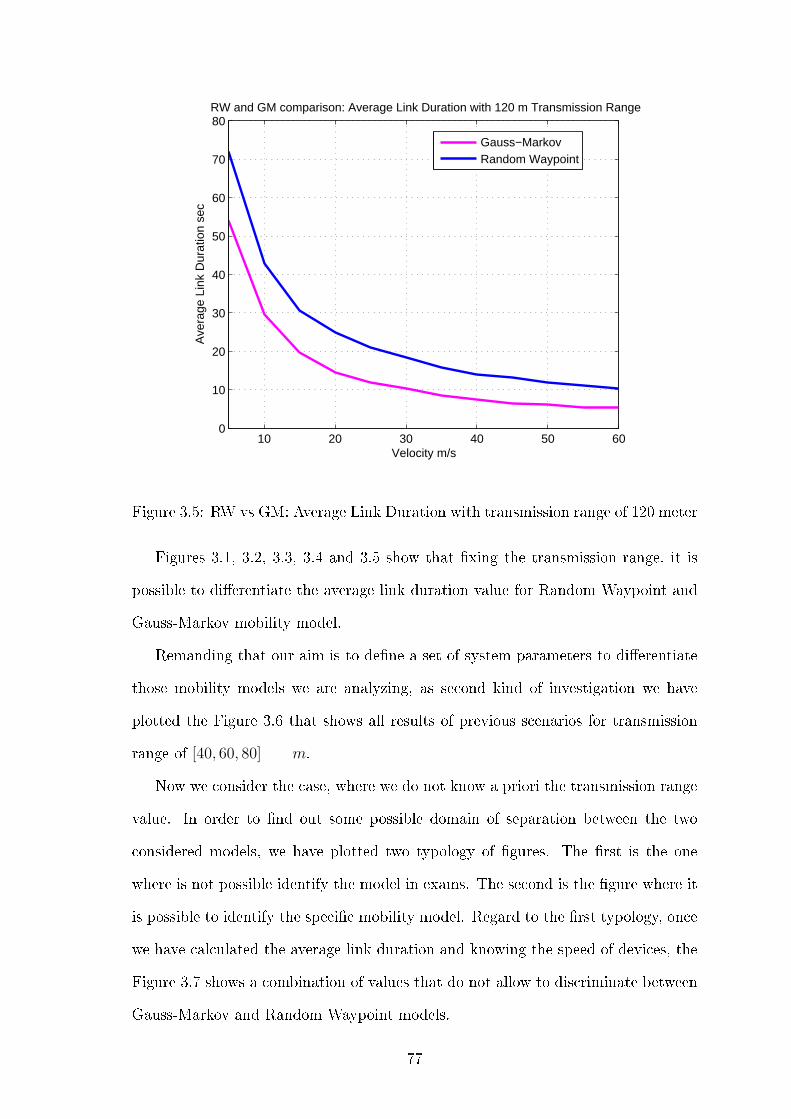
10 20 30 40 50 600
10
20
30
40
50
60
70
80
Velocity m/s
Ave
rage
Lin
k D
urat
ion
sec
RW and GM comparison: Average Link Duration with 120 m Transmission Range
Gauss−MarkovRandom Waypoint
Figure 3.5: RW vs GM: Average Link Duration with transmission range of 120 meter
Figures 3.1, 3.2, 3.3, 3.4 and 3.5 show that �xing the transmission range, it is
possible to di�erentiate the average link duration value for Random Waypoint and
Gauss-Markov mobility model.
Remanding that our aim is to de�ne a set of system parameters to di�erentiate
those mobility models we are analyzing, as second kind of investigation we have
plotted the Figure 3.6 that shows all results of previous scenarios for transmission
range of [40, 60, 80] m.
Now we consider the case, where we do not know a priori the transmission range
value. In order to �nd out some possible domain of separation between the two
considered models, we have plotted two typology of �gures. The �rst is the one
where is not possible identify the model in exams. The second is the �gure where it
is possible to identify the speci�c mobility model. Regard to the �rst typology, once
we have calculated the average link duration and knowing the speed of devices, the
Figure 3.7 shows a combination of values that do not allow to discriminate between
Gauss-Markov and Random Waypoint models.
77
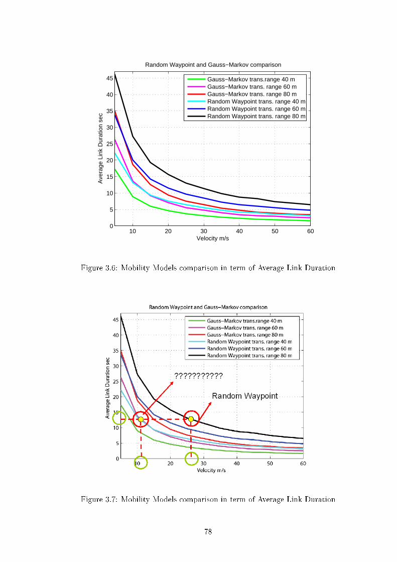
10 20 30 40 50 600
5
10
15
20
25
30
35
40
45
Velocity m/s
Ave
rage
Lin
k D
urat
ion
sec
Random Waypoint and Gauss−Markov comparison
Gauss−Markov trans.range 40 mGauss−Markov trans. range 60 mGauss−Markov trans. range 80 mRandom Waypoint trans. range 40 mRandom Waypoint trans. range 60 mRandom Waypoint trans. range 80 m
Figure 3.6: Mobility Models comparison in term of Average Link Duration
Figure 3.7: Mobility Models comparison in term of Average Link Duration
78
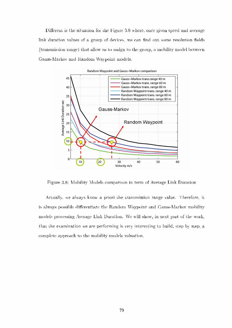
Di�erent is the situation for the Figure 3.8 where, once given speed and average
link duration values of a group of devices, we can �nd out some resolution �elds
(transmission range) that allow us to assign to the group, a mobility model between
Gauss-Markov and Random Waypoint models.
Figure 3.8: Mobility Models comparison in term of Average Link Duration
Actually, we always know a priori the transmission range value. Therefore, it
is always possible di�erentiate the Random Waypoint and Gauss-Markov mobility
models processing Average Link Duration. We will show, in next part of the work,
that the examination we are performing is very interesting to build, step by step, a
complete approach to the mobility models valuation.
79
Chapter 4
Mobility Model Estimation: The
�Guess Who� Algorithm
We have showed in the third chapter how is possible to di�erentiate two mobility
models by processing one mobility metric. In particular, we have performed the
evaluation of the average link duration for Gauss-Markov and Random Waypoint
mobility models. Moreover, in the same chapter we have performed other mobility
metrics and an analytic representation of Random Waypoint mobility model. Even
if a single mobility metric does not univocally identify a mobility model, a network
entity could use several mobility metrics and information to identify the mobility
model of a group of devices. Moreover, in order to resolve two fundamental issues
of WSNs, such as energy waste and resource conserving, we have proposed a simple
approach that allows us to estimate the mobility model. For example, in the Figure
4.4, we consider a WSNs area, covered by several anchor nodes, where there are two
groups, A and B, that have two di�erent mobility behaviors; the movement of the
group A could be approximate with the Random Waypoint mobility model and the
movement of the group B with the Gauss Markov one.
Figures 4.2 and 4.3 show that at the end of a �xed time interval, the group A
could have more chances to reach a further cell than the group B. So doing, thanks
to the knowledge of the mobility model of a group, an anchor node could estimate
80
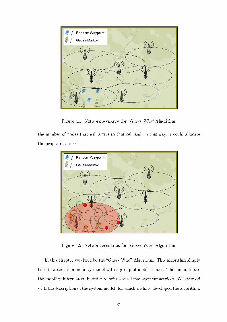
Figure 4.1: Network scenarios for �Guess Who� Algorithm.
the number of nodes that will arrive to that cell and, in this way, it could allocate
the proper resources.
Figure 4.2: Network scenarios for �Guess Who� Algorithm.
In this chapter we describe the �Guess Who� Algorithm. This algorithm simply
tries to associate a mobility model with a group of mobile nodes. The aim is to use
the mobility information in order to o�er several management services. We start o�
with the description of the system model, for which we have developed the algorithm,
81
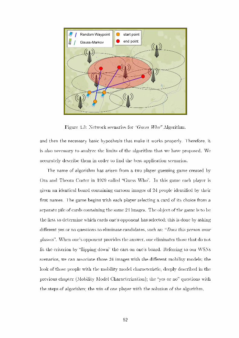
Figure 4.3: Network scenarios for �Guess Who� Algorithm.
and then the necessary basic hypothesis that make it works properly. Therefore, it
is also necessary to analyze the limits of the algorithm that we have proposed. We
accurately describe them in order to �nd the best application scenarios.
The name of algorithm has arisen from a two-player guessing game created by
Ora and Theora Coster in 1979 called �Guess Who�. In this game each player is
given an identical board containing cartoon images of 24 people identi�ed by their
�rst names. The game begins with each player selecting a card of its choice from a
separate pile of cards containing the same 24 images. The object of the game is to be
the �rst to determine which cards one's opponent has selected; this is done by asking
di�erent yes or no questions to eliminate candidates, such as: �Does this person wear
glasses�. When one's opponent provides the answer, one eliminates those that do not
�t the criterion by ��ipping down� the cars on one's board. Referring to our WSNs
scenarios, we can associate those 24 images with the di�erent mobility models; the
look of those people with the mobility model characteristic, deeply described in the
previous chapter (Mobility Model Characterization); the �yes or no� questions with
the steps of algorithm; the win of one player with the solution of the algorithm.
82
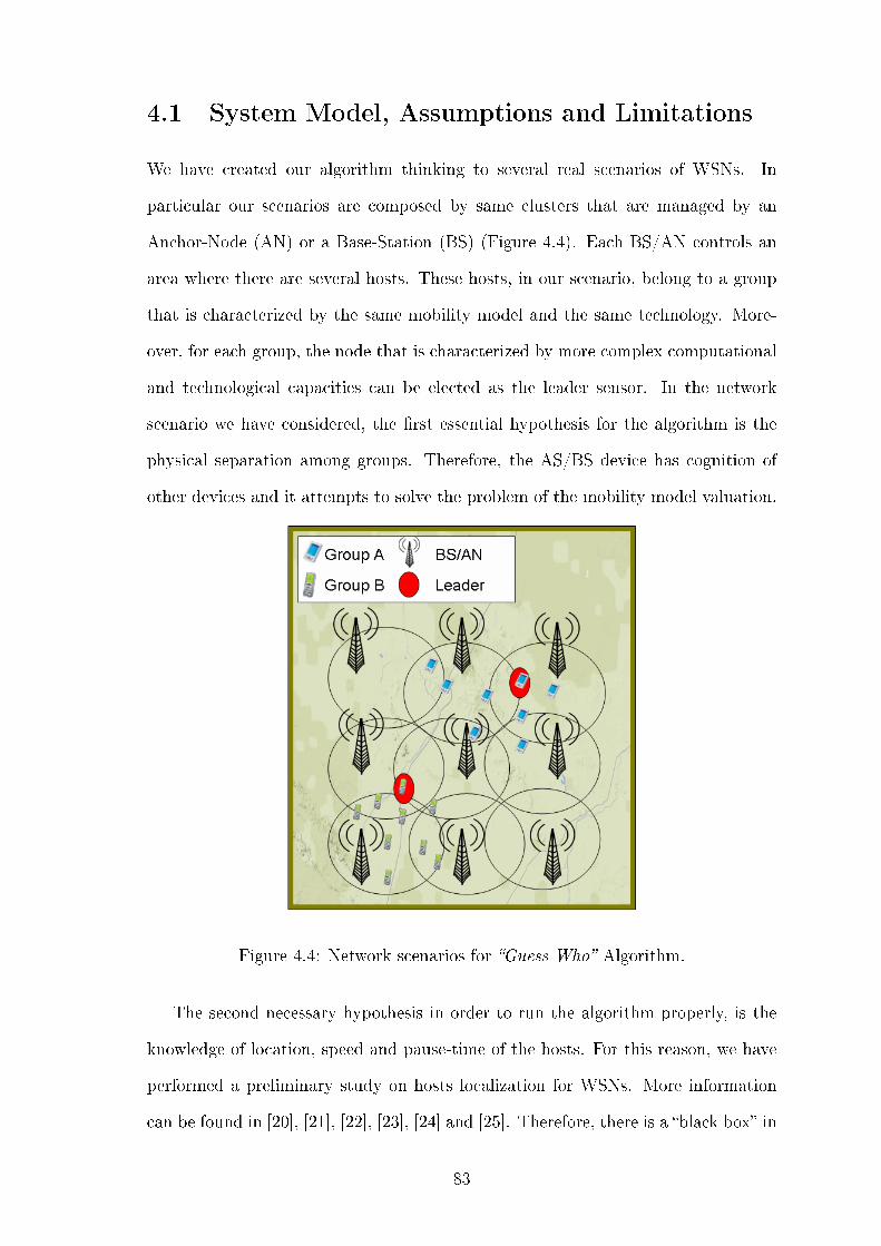
4.1 System Model, Assumptions and Limitations
We have created our algorithm thinking to several real scenarios of WSNs. In
particular our scenarios are composed by same clusters that are managed by an
Anchor-Node (AN) or a Base-Station (BS) (Figure 4.4). Each BS/AN controls an
area where there are several hosts. These hosts, in our scenario, belong to a group
that is characterized by the same mobility model and the same technology. More-
over, for each group, the node that is characterized by more complex computational
and technological capacities can be elected as the leader sensor. In the network
scenario we have considered, the �rst essential hypothesis for the algorithm is the
physical separation among groups. Therefore, the AS/BS device has cognition of
other devices and it attempts to solve the problem of the mobility model valuation.
Figure 4.4: Network scenarios for �Guess Who� Algorithm.
The second necessary hypothesis in order to run the algorithm properly, is the
knowledge of location, speed and pause-time of the hosts. For this reason, we have
performed a preliminary study on hosts localization for WSNs. More information
can be found in [20], [21], [22], [23], [24] and [25]. Therefore, there is a �black box� in
83

the WSN core which o�ers to the algorithm some information such as coordinates,
speeds and pause-times.
The device, that performs our algorithm, is able to work regardless of compu-
tation resources and also able to communicate with the network of sinks. For this
reason we suppose a link communication between the group leader and the BS\AN
device.
Limitations of our algorithm are clearly visible: (i) we have to consider time and
overhead that �black-box� needs to calculate mobility information; (ii) there is the
issue of error accuracy of mobility information valuation.
The aim of our work is not to �nd out the best algorithm but to develop a simple
approach to solve a problem of mobility model estimation.
4.2 Look Up Table Based on Estimation Approach
Before of continuing the description of the proposed algorithm, we want to describe
foundations of our mobility model valuation. For this reason we have designed the
table, shown in the Figure 4.5, which summarizes some mobility models and mobility
metrics used by the �Guess Who� algorithm.
Figure 4.5: Table of �Estimation Approach�.
84
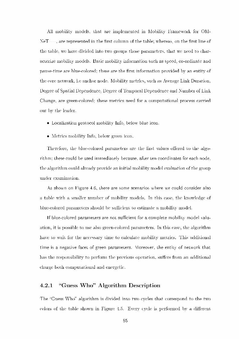
All mobility models, that are implemented in Mobility Framework for OM-
NeT++, are represented in the �rst column of the table; whereas, on the �rst line of
the table, we have divided into two groups those parameters, that we need to char-
acterize mobility models. Basic mobility information such as speed, co-ordinate and
pause-time are blue-colored; these are the �rst information provided by an entity of
the core network, i.e anchor node. Mobility metrics, such as Average Link Duration,
Degree of Spatial Dependence, Degree of Temporal Dependence and Number of Link
Change, are green-colored; these metrics need for a computational process carried
out by the leader.
• Localization protocol mobility Info, below blue icon.
• Metrics mobility Info, below green icon.
Therefore, the blue-colored parameters are the �rst values o�ered to the algo-
rithm; these could be used immediately because, after ten coordinates for each node,
the algorithm could already provide an initial mobility model evaluation of the group
under examination.
As shown on Figure 4.6, there are some scenarios where we could consider also
a table with a smaller number of mobility models. In this case, the knowledge of
blue-colored parameters should be su�cient to estimate a mobility model.
If blue-colored parameters are not su�cient for a complete mobility model valu-
ation, it is possible to use also green-colored parameters. In this case, the algorithm
have to wait for the necessary time to calculate mobility metrics. This additional
time is a negative facet of green parameters. Moreover, the entity of network that
has the responsibility to perform the previous operation, su�ers from an additional
charge both computational and energetic.
4.2.1 �Guess Who� Algorithm Description
The �Guess Who� algorithm is divided into two cycles that correspond to the two
colors of the table shown in Figure 4.5. Every cycle is performed by a di�erent
85
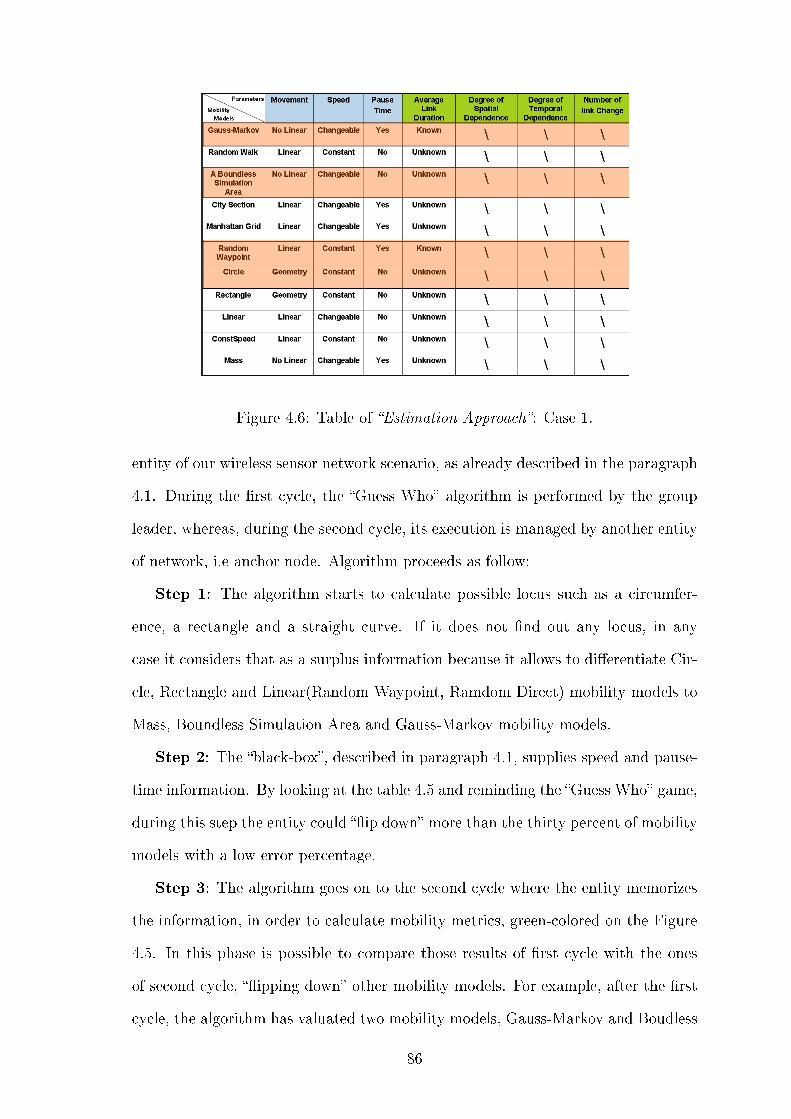
Figure 4.6: Table of �Estimation Approach�: Case 1.
entity of our wireless sensor network scenario, as already described in the paragraph
4.1. During the �rst cycle, the �Guess Who� algorithm is performed by the group
leader, whereas, during the second cycle, its execution is managed by another entity
of network, i.e anchor node. Algorithm proceeds as follow:
Step 1: The algorithm starts to calculate possible locus such as a circumfer-
ence, a rectangle and a straight curve. If it does not �nd out any locus, in any
case it considers that as a surplus information because it allows to di�erentiate Cir-
cle, Rectangle and Linear(Random Waypoint, Ramdom Direct) mobility models to
Mass, Boundless Simulation Area and Gauss-Markov mobility models.
Step 2: The �black-box�, described in paragraph 4.1, supplies speed and pause-
time information. By looking at the table 4.5 and reminding the �Guess Who� game,
during this step the entity could ��ip down� more than the thirty percent of mobility
models with a low error percentage.
Step 3: The algorithm goes on to the second cycle where the entity memorizes
the information, in order to calculate mobility metrics, green-colored on the Figure
4.5. In this phase is possible to compare those results of �rst cycle with the ones
of second cycle, ��ipping down� other mobility models. For example, after the �rst
cycle, the algorithm has valuated two mobility models, Gauss-Markov and Boudless
86
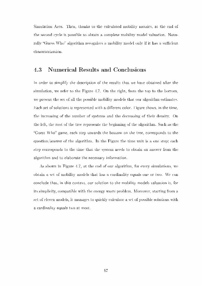
Simulation Area. Then, thanks to the calculated mobility metrics, at the end of
the second cycle it possible to obtain a complete mobility model valuation. Natu-
rally �Guess Who� algorithm recognizes a mobility model only if it has a su�cient
characterization.
4.3 Numerical Results and Conclusions
In order to simplify the description of the results that we have obtained after the
simulation, we refer to the Figure 4.7. On the right, from the top to the bottom,
we present the set of all the possible mobility models that our algorithm estimates.
Each set of solutions is represented with a di�erent color. Figure shows, in the time,
the increasing of the number of systems and the decreasing of their density. On
the left, the root of the tree represents the beginning of the algorithm. Such as the
�Guess Who� game, each step towards the bottom on the tree, corresponds to the
question/answer of the algorithm. In the Figure the time unit is a one step; each
step corresponds to the time that the system needs to obtain an answer from the
algorithm and to elaborate the necessary information.
As shown in Figure 4.7, at the end of our algorithm, for every simulations, we
obtain a set of mobility models that has a cardinality equals one or two. We can
conclude that, in this context, our solution to the mobility models valuation is, for
its simplicity, compatible with the energy waste problem. Moreover, starting from a
set of eleven models, it manages to quickly calculate a set of possible solutions with
a cardinality equals two at most.
87
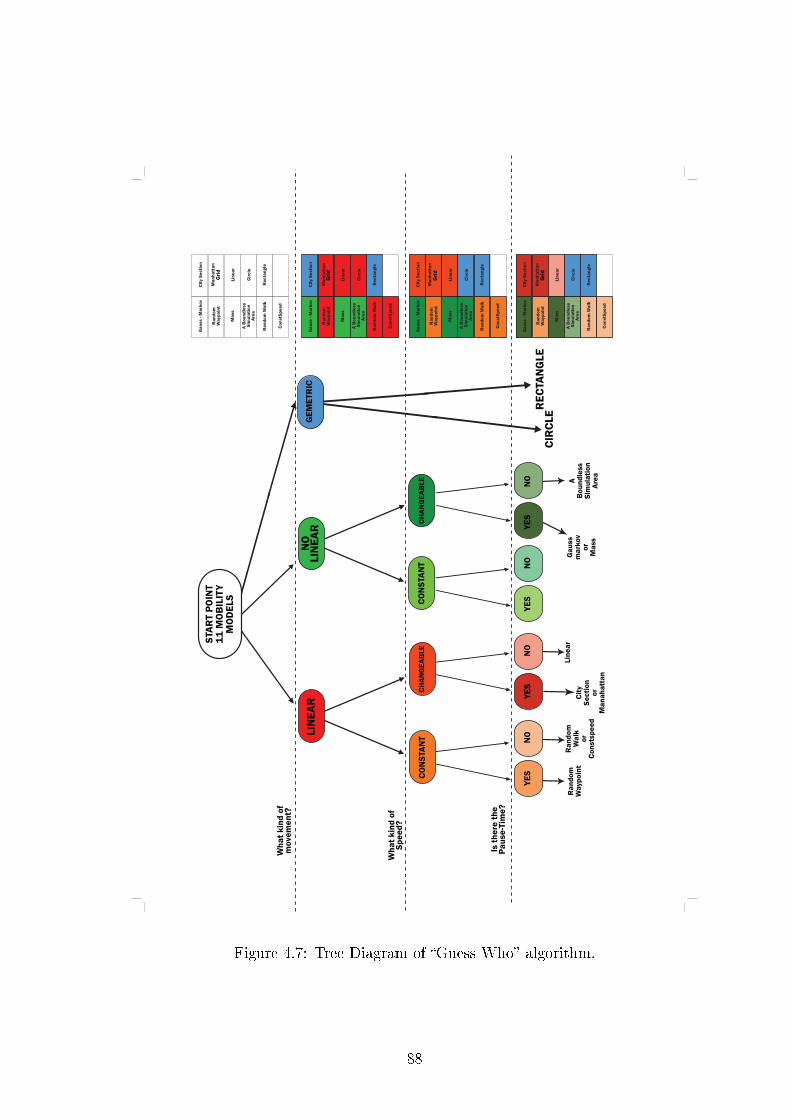
Figure 4.7: Tree Diagram of �Guess Who� algorithm.
88
Chapter 5
Overview of simulation environment
Performance evaluation is carried out in the Object-oriented Modular Event Net-
work (OMNeT++) simulator , that provides basic machinery and tools to write
all components of queuing networks. Speci�c application areas are supported by
various simulations models and frameworks such as the Mobility Framework. These
models are developed completely independently of OMNeT++. In particular we
have worked with Mobility Framework that supports wireless and mobile simulation
within OMNeT++.
5.0.1 OMNeT++
OMNeT++ was designed from the beginnings to support network simulation on a
large scale. This objective lead to following main design requirements:
• Enable large-scale simulation: simulation models need to be hierarchical,
and built from reusable components as much as possible
• Easy debugging: the simulation software should facilitate visualizing and
debugging of simulation models in order to reduce debugging time, which
traditionally takes up a large percentage of simulation projects. (The same
feature set is also useful for educational use of the software)
• Modular simulator software: The simulation software itself should be mod-
89
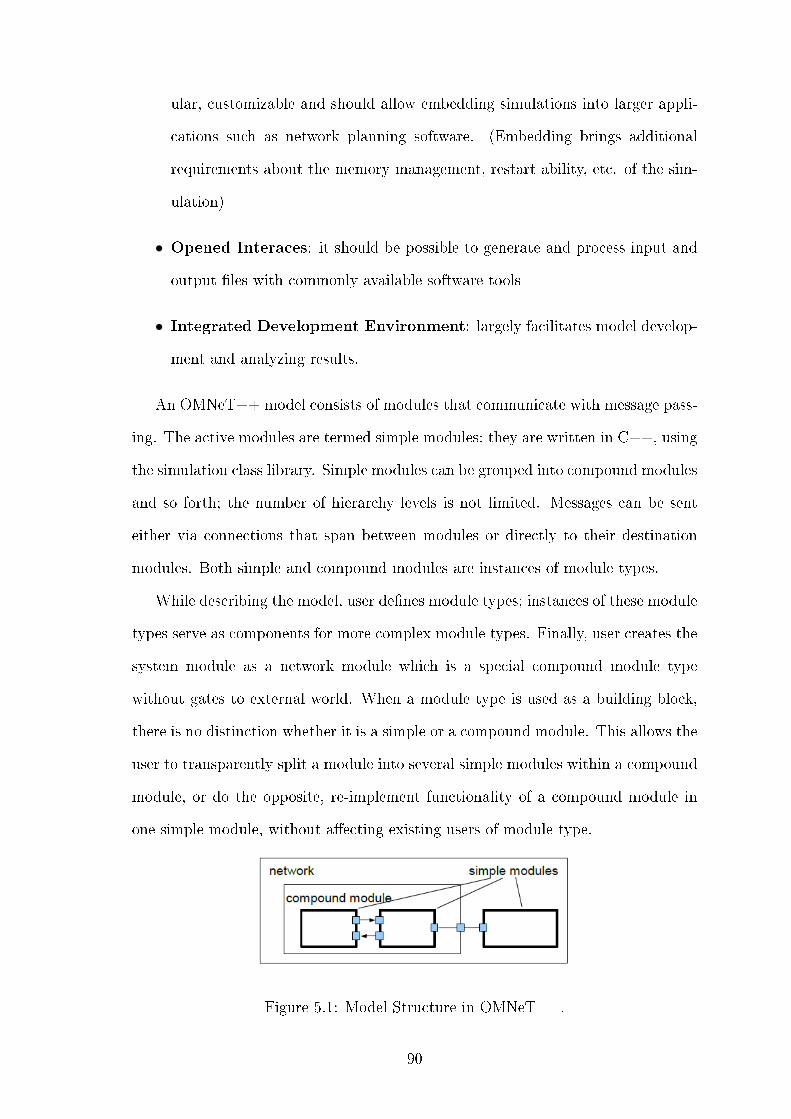
ular, customizable and should allow embedding simulations into larger appli-
cations such as network planning software. (Embedding brings additional
requirements about the memory management, restart ability, etc. of the sim-
ulation)
• Opened Interaces: it should be possible to generate and process input and
output �les with commonly available software tools
• Integrated Development Environment: largely facilitates model develop-
ment and analyzing results.
An OMNeT++ model consists of modules that communicate with message pass-
ing. The active modules are termed simple modules; they are written in C++, using
the simulation class library. Simple modules can be grouped into compound modules
and so forth; the number of hierarchy levels is not limited. Messages can be sent
either via connections that span between modules or directly to their destination
modules. Both simple and compound modules are instances of module types.
While describing the model, user de�nes module types; instances of these module
types serve as components for more complex module types. Finally, user creates the
system module as a network module which is a special compound module type
without gates to external world. When a module type is used as a building block,
there is no distinction whether it is a simple or a compound module. This allows the
user to transparently split a module into several simple modules within a compound
module, or do the opposite, re-implement functionality of a compound module in
one simple module, without a�ecting existing users of module type.
Figure 5.1: Model Structure in OMNeT++.
90
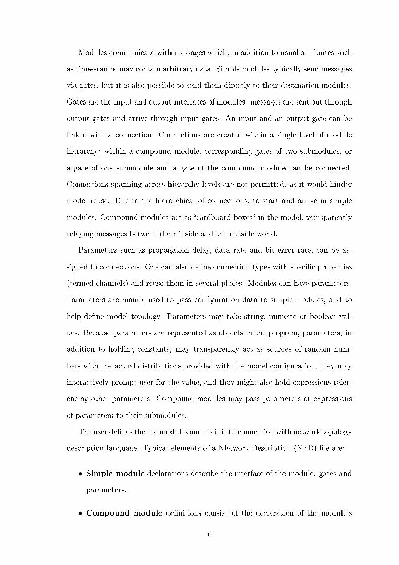
Modules communicate with messages which, in addition to usual attributes such
as time-stamp, may contain arbitrary data. Simple modules typically send messages
via gates, but it is also possible to send them directly to their destination modules.
Gates are the input and output interfaces of modules: messages are sent out through
output gates and arrive through input gates. An input and an output gate can be
linked with a connection. Connections are created within a single level of module
hierarchy: within a compound module, corresponding gates of two submodules, or
a gate of one submodule and a gate of the compound module can be connected.
Connections spanning across hierarchy levels are not permitted, as it would hinder
model reuse. Due to the hierarchical of connections, to start and arrive in simple
modules. Compound modules act as �cardboard boxes� in the model, transparently
relaying messages between their inside and the outside world.
Parameters such as propagation delay, data rate and bit error rate, can be as-
signed to connections. One can also de�ne connection types with speci�c properties
(termed channels) and reuse them in several places. Modules can have parameters.
Parameters are mainly used to pass con�guration data to simple modules, and to
help de�ne model topology. Parameters may take string, numeric or boolean val-
ues. Because parameters are represented as objects in the program, parameters, in
addition to holding constants, may transparently act as sources of random num-
bers with the actual distributions provided with the model con�guration, they may
interactively prompt user for the value, and they might also hold expressions refer-
encing other parameters. Compound modules may pass parameters or expressions
of parameters to their submodules.
The user de�nes the the modules and their interconnection with network topology
description language. Typical elements of a NEtwork Description (NED) �le are:
• Simple module declarations describe the interface of the module: gates and
parameters.
• Compound module de�nitions consist of the declaration of the module's
91
external interface(gates and parameters), and the de�nition of submodules
and their interconnection.
• Network de�nitions are compound modules that qualify as self-contained
simulation models.
The following features have been introduced.
Inheritance: Modules and channels can now be subclassed. Derived modules
and channels may add new parameters, gates, and (in the case of compound mod-
ules) new submodules and connections. They may set existing parameters to a
speci�c value, and also set the gate size of a gate vector.
Interfaces: Module and channel interfaces can be used as a placeholder where
normally a module or channel type would be used, and the concrete module or
channel type is determined at network setup time by a parameter. Concrete module
types have to �implement� the interface they can substitute.
Packages: To address name clashes between di�erent models and to simplify
specifying which NED �les are needed by a speci�c simulation model, a Java-like
package structure was introduced into the NED language.
Inner types: Channel types and module types used locally by a compound
module can now be de�ned within the compound module, in order to reduce names-
pace pollution.
OMNeT++ package includes an Integrated Development Environment which
contains a graphical editor using NED as its native �le format; moreover, the editor
can work with arbitrary, even hand-written NED code. Editor is a fully two-way
tool, i.e. user can edit the network topology either graphically or in NED source
view, and switch between two views at any time.
This is made possible by design decisions about the NED language itself. First,
NED is a declarative language, and as such, it does not use an imperative program-
ming language for de�ning the internal structure of a compound module. Allowing
arbitrary programming constructs would make it practically infeasible to write two-
92
Figure 5.2: OMNeT++ an example of working environment.
way graphical editors which could work directly with both generated and hand-made
NED �les. (Generally, editor would need AI capability to understand the code.)
Most graphical editors only allow the creation of �xed topologies. However, NED
contains declarative constructs (resembling loops and conditionals in imperative lan-
guages), which enable parametric topologies: it is possible to create common regular
topologies such as ring, grid, star, tree, hypercube, or random interconnection whose
parameters (size, etc.) are passed in numeric-valued parameters.
5.0.2 Mobility-Framework
This framework is intended to support wireless and mobile simulations within OM-
NeT++ [18]. The core framework implements the support for node mobility, dy-
namic connection management and a wireless channel model. Additionally the core
framework provides basic modules that can be derived in order to implement own
modules. With this concept a programmer can easily develop own protocol imple-
mentations for the Mobility Framework (MF) without having to deal with the neces-
sary interface and inter-operability stu�. The two core components of the Mobility
93
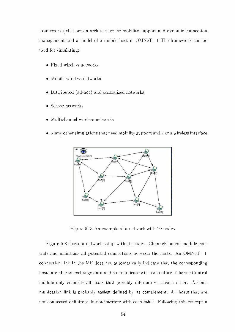
Framework (MF) are an architecture for mobility support and dynamic connection
management and a model of a mobile host in OMNeT++.The framework can be
used for simulating:
• Fixed wireless networks
• Mobile wireless networks
• Distributed (ad-hoc) and centralized networks
• Sensor networks
• Multichannel wireless networks
• Many other simulations that need mobility support and / or a wireless interface
Figure 5.3: An example of a network with 10 nodes.
Figure 5.3 shows a network setup with 10 nodes. ChannelControl module con-
trols and maintains all potential connections between the hosts. An OMNeT++
connection link in the MF does not automatically indicate that the corresponding
hosts are able to exchange data and communicate with each other. ChannelControl
module only connects all hosts that possibly interfere with each other. A com-
munication link is probably easiest de�ned by its complement: All hosts that are
not connected de�nitely do not interfere with each other. Following this concept a
94
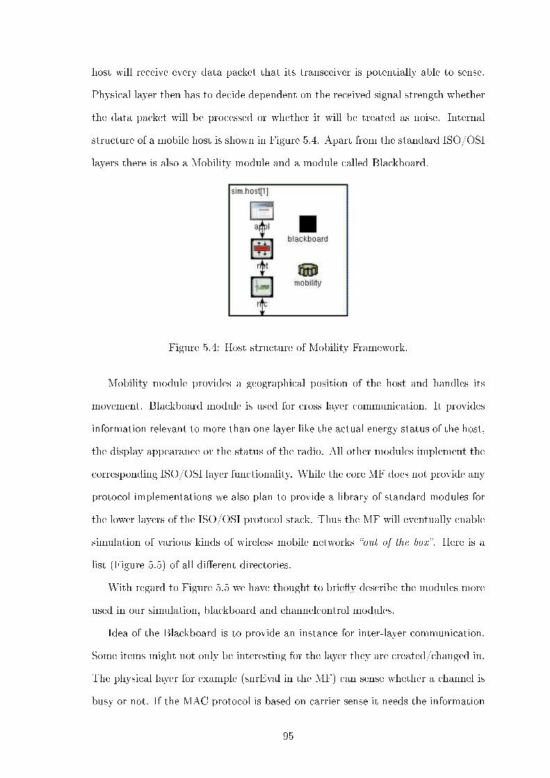
host will receive every data packet that its transceiver is potentially able to sense.
Physical layer then has to decide dependent on the received signal strength whether
the data packet will be processed or whether it will be treated as noise. Internal
structure of a mobile host is shown in Figure 5.4. Apart from the standard ISO/OSI
layers there is also a Mobility module and a module called Blackboard.
Figure 5.4: Host structure of Mobility Framework.
Mobility module provides a geographical position of the host and handles its
movement. Blackboard module is used for cross layer communication. It provides
information relevant to more than one layer like the actual energy status of the host,
the display appearance or the status of the radio. All other modules implement the
corresponding ISO/OSI layer functionality. While the core MF does not provide any
protocol implementations we also plan to provide a library of standard modules for
the lower layers of the ISO/OSI protocol stack. Thus the MF will eventually enable
simulation of various kinds of wireless mobile networks �out of the box�. Here is a
list (Figure 5.5) of all di�erent directories.
With regard to Figure 5.5 we have thought to brie�y describe the modules more
used in our simulation, blackboard and channelcontrol modules.
Idea of the Blackboard is to provide an instance for inter-layer communication.
Some items might not only be interesting for the layer they are created/changed in.
The physical layer for example (snrEval in the MF) can sense whether a channel is
busy or not. If the MAC protocol is based on carrier sense it needs the information
95
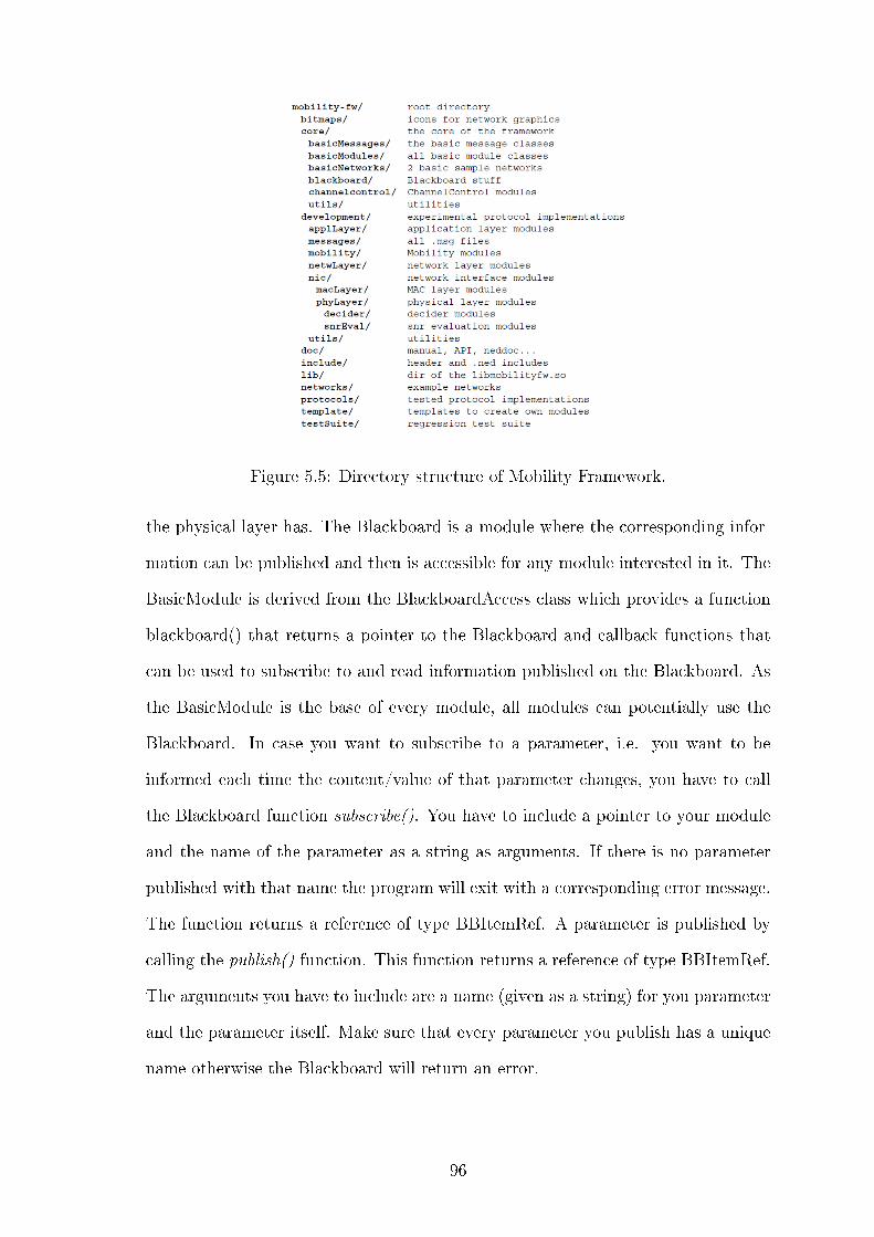
Figure 5.5: Directory structure of Mobility Framework.
the physical layer has. The Blackboard is a module where the corresponding infor-
mation can be published and then is accessible for any module interested in it. The
BasicModule is derived from the BlackboardAccess class which provides a function
blackboard() that returns a pointer to the Blackboard and callback functions that
can be used to subscribe to and read information published on the Blackboard. As
the BasicModule is the base of every module, all modules can potentially use the
Blackboard. In case you want to subscribe to a parameter, i.e. you want to be
informed each time the content/value of that parameter changes, you have to call
the Blackboard function subscribe(). You have to include a pointer to your module
and the name of the parameter as a string as arguments. If there is no parameter
published with that name the program will exit with a corresponding error message.
The function returns a reference of type BBItemRef. A parameter is published by
calling the publish() function. This function returns a reference of type BBItemRef.
The arguments you have to include are a name (given as a string) for you parameter
and the parameter itself. Make sure that every parameter you publish has a unique
name otherwise the Blackboard will return an error.
96
ChannelControl module is responsible for establishing communication channels
between Host modules that are within communication distance and tearing down
these connections once they loose connectivity again. The loss of connectivity can be
due to mobility (i.e. the Hosts move too far apart) or due to a change in transmission
power or a crashed Host etc. We decided to keep the concept of links between
Host modules, as opposed to direct message passing, since visible communication
paths are an important source of (debugging) information in early development part.
Unfortunately, in OMNeT++ distinct links between modules require at least two
gate objects for each module, one in- and one out- gate (and for each submodule as
well). For our MF the minimal number of gates per link is six since the Nic module
is embedded within the Host module and is itself subdivided into an SnrEval, a
Decider module and a Mac module. To make sure to have enough gates even in the
worst case scenario (all Hosts are directly connected), each Host module needs at
least two pairs of gates for every single Host module in the network.
A more memory-e�cient approach is to create gates dynamically which is the
way we decided to go. Gates are not allocated in bulk upon initialization of the
network but created dynamically ondemand. Each Host module maintains two lists
one for the free in-gates and one for the free out-gates. Once ChannelControl wants
to establish a link between two Hosts, it �rst checks the gate lists in both Hosts
whether free gates are available and only if no free gate was found a new one is
created. Upon link break ChannelControl tears down the connection and adds the
newly freed gates to the corresponding gate list. With this approach we minimize
the memory needed without increasing the computational overhead to create and
destroy gates too much. In wireless network simulations is not only important thatr
two hosts are connected (i.e. can communicate each other) but also that two hosts
can interfere each other. That is why the term connection gets a slightly di�erent
meaning for our MF. Upon initialization, the Channel-Control module determines
the maximum interference distance based on global network parameters such as the
carrier frequency of the channel, the maximal possible sending power and other
97
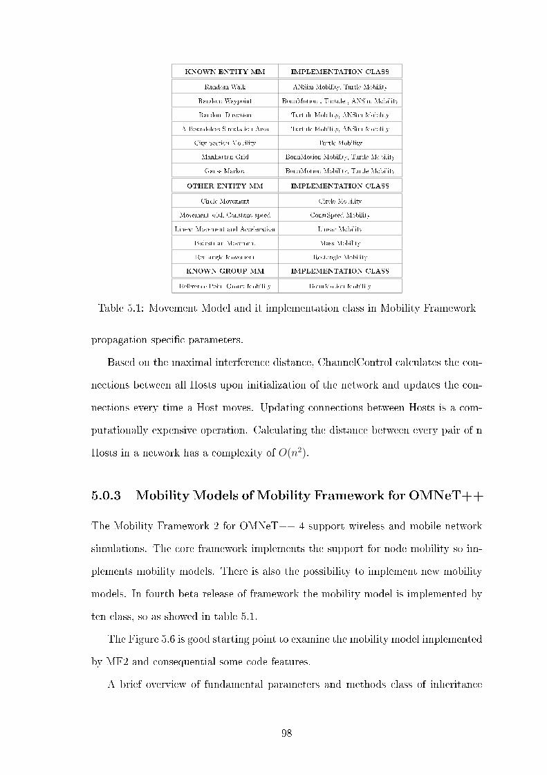
KNOWN ENTITY MM IMPLEMENTATION CLASS
Random Walk ANSim Mobility, Turtle Mobility
Random Waypoint BonnMotion , Turtule , ANSim Mobility
Random Direction Turtule Mobility, ANSim Mobility
A Boundeless Simulation Area Turtule Mobility, ANSim Mobility
City Section Mobility Turtle Mobility
Manhattan Grid BonnMotion Mobility, Turtle Mobility
Gauss-Markov BonnMotion Mobility, Turtle Mobility
OTHER ENTITY MM IMPLEMENTATION CLASS
Circle Movement Circle Mobility
Movement with Constant speed ConstSpeed Mobility
Linear Movement and Acceleration Linear Mobility
Pedestrian Movement Mass Mobility
Rectangle Movement Rectangle Mobility
KNOWN GROUP MM IMPLEMENTATION CLASS
Reference Point Group Mobility BonnMotion Mobility
Table 5.1: Movement Model and it implementation class in Mobility Framework
propagation speci�c parameters.
Based on the maximal interference distance, ChannelControl calculates the con-
nections between all Hosts upon initialization of the network and updates the con-
nections every time a Host moves. Updating connections between Hosts is a com-
putationally expensive operation. Calculating the distance between every pair of n
Hosts in a network has a complexity of O(n2).
5.0.3 Mobility Models of Mobility Framework for OMNeT++
The Mobility Framework 2 for OMNeT++ 4 support wireless and mobile network
simulations. The core framework implements the support for node mobility so im-
plements mobility models. There is also the possibility to implement new mobility
models. In fourth beta release of framework the mobility model is implemented by
ten class, so as showed in table 5.1.
The Figure 5.6 is good starting point to examine the mobility model implemented
by MF2 and consequential some code features.
A brief overview of fundamental parameters and methods class of inheritance
98
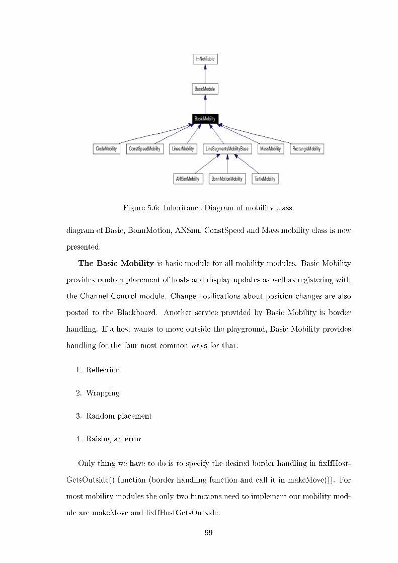
Figure 5.6: Inheritance Diagram of mobility class.
diagram of Basic, BonnMotion, ANSim, ConstSpeed and Mass mobility class is now
presented.
The Basic Mobility is basic module for all mobility modules. Basic Mobility
provides random placement of hosts and display updates as well as registering with
the Channel Control module. Change noti�cations about position changes are also
posted to the Blackboard. Another service provided by Basic Mobility is border
handling. If a host wants to move outside the playground, Basic Mobility provides
handling for the four most common ways for that:
1. Re�ection
2. Wrapping
3. Random placement
4. Raising an error
Only thing we have to do is to specify the desired border handling in �xIfHost-
GetsOutside() function (border handling function and call it in makeMove()). For
most mobility modules the only two functions need to implement our mobility mod-
ule are makeMove and �xIfHostGetsOutside.
99
BonnMotion class uses the native �le format of BonnMotion ??. BonnMotion is
a Java software which creates and analyzes mobility scenario. A mobility model
avaible with BonnMotion �le are:
1. The Random Waypoint model
2. The Manhattan Grid model
3. Gauss-Markov models
4. The Reference Point Group Mobility Model
5. Static scenario
BonnMotion programm produce a xml �le that is a plain text �le, where every
line describes the motion of one host. A line consists of one or more (t, x, y) triplets
of real numbers, like: (t1, x1, y1); (t2, x2, y2); (t3, x3, y3); (t4, x4, y4)...
ConstSpeed Mobility does not use one of the standard approaches. The
user can de�ne a velocity for each Host and an update interval. If the velocity
is greater than zero (the Host is not stazionary) the ConstSpeed Mobility module
calculates a random target position for the Host. Depending to the update interval
and velocity it calculates the number of steps to reach the destination and the
step-size. Every update interval ConstSpeedMobility calculates the new position on
its way to the target position and updates the display. Once the target position
is reaches ConstSpeed Mobility calculates a new target position. With following
parameters, speci�ed in omnetpp.ini, it is possible control all movement of hosts.
1. vHost : Speed of a host [m\s]
2. updateInterval : Time interval to update the hosts position
3. (x,y) : Starting position of the host, -1 = random
Ad-Hoc Network Simulation (ANSim) mobility uses the position change
elements of the Ad-Hoc Network Simulation (ANSim) tool's trace �le. The trace
100
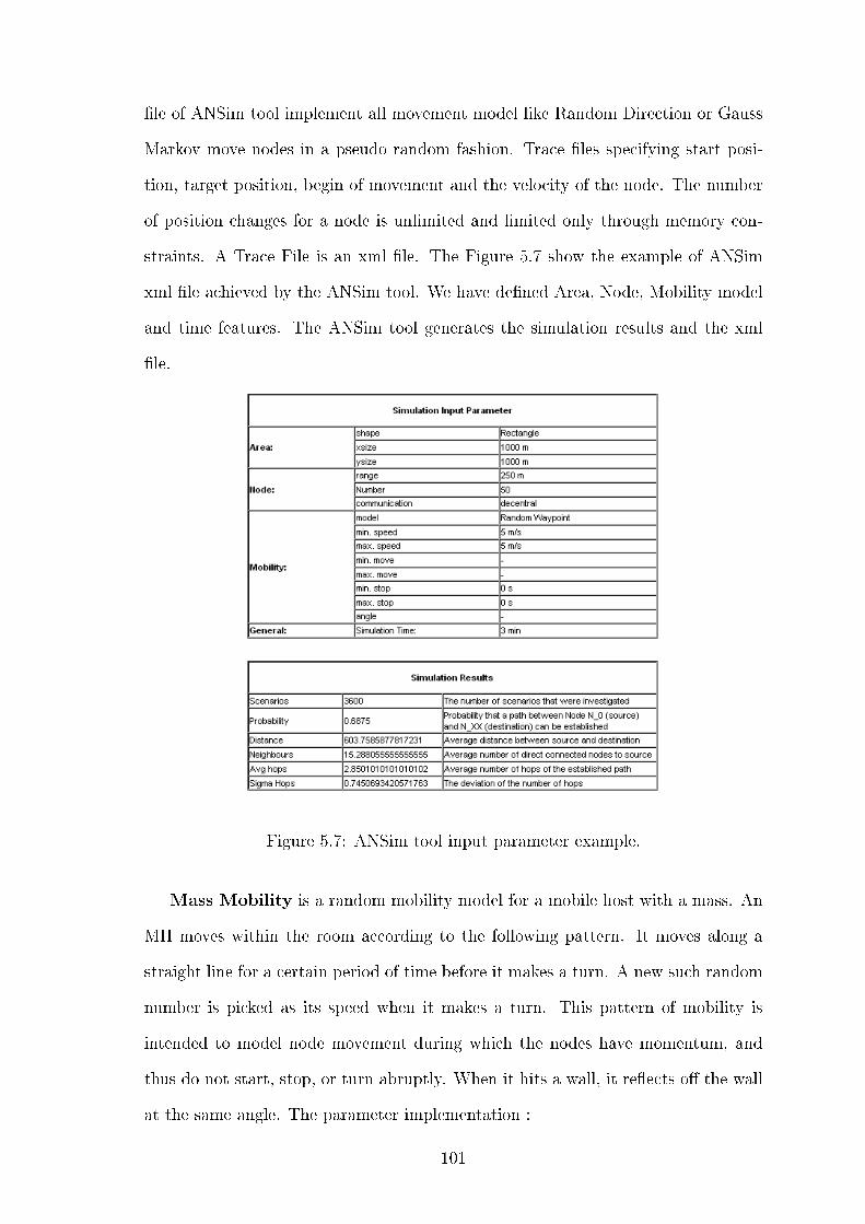
�le of ANSim tool implement all movement model like Random Direction or Gauss
Markov move nodes in a pseudo random fashion. Trace �les specifying start posi-
tion, target position, begin of movement and the velocity of the node. The number
of position changes for a node is unlimited and limited only through memory con-
straints. A Trace File is an xml �le. The Figure 5.7 show the example of ANSim
xml �le achieved by the ANSim tool. We have de�ned Area, Node, Mobility model
and time features. The ANSim tool generates the simulation results and the xml
�le.
Figure 5.7: ANSim tool input parameter example.
Mass Mobility is a random mobility model for a mobile host with a mass. An
MH moves within the room according to the following pattern. It moves along a
straight line for a certain period of time before it makes a turn. A new such random
number is picked as its speed when it makes a turn. This pattern of mobility is
intended to model node movement during which the nodes have momentum, and
thus do not start, stop, or turn abruptly. When it hits a wall, it re�ects o� the wall
at the same angle. The parameter implementation :
101

1. (x,y): x and y starting point of the node
2. changeInterval a frequency of changing speed and angle (can random)[s]
3. changeAngleBy a change angle by this much (can be random) [deg]
4. speed (can be random, updated every changeInterval) [m/s]
5. updateInterval
102
Chapter 6
Conclusions and future work
In conclusion, we could divide this master thesis into four main parts. First, we have
proposed those two mobility models that better �t with WSNs scenarios, that are
the core of this master thesis. Second, we have investigated on the mobility models
characterization. Third, we have evaluated the impact of investigated mobility mod-
els on mobility metrics. Fourth, we have proposed a simple and e�cient algorithm,
the �Guess Who�, to estimate the best �tting mobility model for a network agent.
Moreover, we have analyzed three important aspects of WSNs.
The �rst one is the importance to distinguish two mobility models typology: (i)
the �ideal� typology, that is used for scenarios where, with a good approximation,
it is possible to adopt those mobility models that already exist in literature; (ii) the
�lifelike� category, that is used for those scenarios where it is necessary to implement
and identify new mobility models that can be used to better describe the movement
of elements of the network.
The second aspect is the valuation of network performances, through those
metrics that give us a characterization of mobility models. These metrics can be
used to recognize and distinguish mobility models among each others.
The third aspect is the estimate of devices mobility of a WSN. Technologies,
that are designed for a WSN, need for more attention because, in this case, both
resources and available energy are limited. The knowledge of the mobility can help
103
the valuation of distributed devices in the network and, therefore, the estimation of
resources that should be allocated in the time.
For the contribution we have made and aspects we have underlined, we think
that it is interesting to study and calculate also all mobility metrics for all mobility
models that we can �nd in literature. Once this characterization will be �nished, a
future work will be to develop new alternative methods to estimate these mobility
models.
104
Bibliography
[1] IEEE 802.15.4 standard, �Part 15.4: Wireless Medium Access Control (MAC)
and Physical Layer (PHY) Speci�cations for Low-Rate Wireless Personal Area
Networks (LR-WPANs)�.
[2] G. Anastasi, M. Conti, M. Di Francesco and A. Passarella, �Energy Conservation
in Wireless Sensor Network� Elsevier, Ad Hoc Netoworks, Vol 7, Issue 6, May
2009, pp. 537-568.
[3] I. Demirkol, C.Ersoy and F.Alagaz, �MAC Protocol for Wireless Sensor Net-
works: A Survey�, IEEE Communications Magazine, Vol. 44, Issue 4, April 2006,
pp. 115-121.
[4] I.F. Akyildiz, W. Su, Y. Sankarasubramaniam and E. Cayirci, �Wireless sensor
networks: a survey�, Elsevier, Computer Network, Vol 38, Number 4, 15 March
2002, pp. 393-422.
[5] P.Baronti, P. Pillai, V. W.C. Chook, S. Chessa, A. Gotta and Y. Fun Hu �Wire-
less sensor networks: A survey on the state of the art and the 802.15.4 and ZigBee
standards�, Elsevier, Computer Network, Vol 30, Issue 7, 26 May 2007, pp. 1655-
1695.
[6] W. Ye, J. Heidemann, D. Estrin, �Medium access control with coordinated adap-
tive sleeping for wireless sensor networks�, IEEE/ACM Transactions on Network-
ing (TON), Vol. 12, Issue 3, June 2004, pp. 493-506.
105
[7] J. Polastre, J. Hill, D. Culler, �Versatile low power media access for wireless
sensor networks�, Proceeding of the 2nd international conference on Embedded
networked system, 2004, Session: Routing and Mac, pp. 95-107.
[8] M. Buettner, G. V. Yee, E. Anderson, R. Han, �X-Mac: a short preamble MAC
protocol for duty-cycled wireless sensor networks�, Proceeding of the 4nd interna-
tional conference on Embedded Networked System, 2003, Los Angeles, California,
USA, Session: Energy-ecci�ent MAC, pp. 171-180.
[9] T.van Dam and K. Langendoen, �An adaptive energy-e�cient MAC protocol
for Wireless Sensor Networks�, Proceeding of the 1nd international conference on
Embedded Networked Sensor System, 2006, Session: Media access control, pp.
307-320.
[10] T. Camp, J. Boleng, and V. Davies, �A Survey of Mobility Models for Ad Hoc
Network Research�, in Wireless Communication and Mobile Computing (WCMC):
Special issue on Mobile Ad Hoc Networking: Research, Trends and Applications,
vol. 2, no. 5, pp. 483-502, 2002.
[11] J. Broch, D. A. Maltz, D. B. Johnson, Y.-C. Hu, and J. Jetcheva, �A per-
formance comparison of multi-hop wireless ad hoc network routing protocols�,
in Proceedings of the Fourth Annual ACM/IEEE International Conference on
Mobile Computing and Networking(Mobicom98), ACM, October 1998.
[12] C. Bettstetter �Mobility Modeling In Wireless Networks: �Categorization,
smooth movement and border e�ects�, in ACM SIGMOBILE Mobile computing
and Communication Review, Vol. 5, Issue 3, July 2001, pp.55-66.
[13] F.Bai, A. Helmy, �rst chapter in the book �Wireless Ad Hoc Networks�, 2004,
Citeseer.
106
[14] B. Liang, Z. J. Haas, �Predictive Distance-Based Mobility Management for
PCS Networks�, in Proceedings of IEEE Information Communications Conference
(INFOCOM 1999), Apr. 1999.
[15] A. Vargas, R. Hornig, �An Overview of The OMNeT++ simulation environ-
ment�, Prooceedings of 1st international conference on Simulation tools and tech-
niques commuincations, NEtworks and System & workshop, session Technical
Program, Marseille (France) 2008, Artcile No.60.
[16] A. Varga, �Omnet++, Discrete Event Simulation System, User Manual�, version
4.
[17] OMNeT++ Communty Homepage htttp://www.omnetpp.org.
[18] M. Lobbers, D. Willkomm, A Mobility Framework for Omnet++, User Manual,
January 12, 2007 version 1.0a4.
[19] Mobility Framework for OMNeT++ Homepage http://mobility-
fw.sourcefourge.net
[20] K. Langendoen, N. Reujers, �Distributed Localization in Wireless Sensor Net-
works: a quantitative comarison�, Elsevier, Computer Networks, Vol. 43, Issue 4,
15 November 2003, pp. 499-518.
[21] A. Baggio, K. Langendoen, �Monte Carlo localization for mobile wireless sensor
networks�,Elsevier, Ad Hoc Networks, Vol.6 Issue 5, July 2008, pp.718-733.
[22] N.B. Priyanatha, H. Balakrishnan, E.D. Demaine and S.Teller, �Mobile-
assisted localization in wireless sensor networks�, in INFOCOM 2005, Miami,
FL,USA,March 2005.
[23] N.Bulus, J. Heidemann, D. Estrin, �GPS-less low cost outdoor localization for
very small devices�, IEEE Personal Communications Magazine, Vol.7, No. 5, Oc-
tober 2000, pp. 28-34.
107
[24] F. Benbadis, T. Friedman, M. Dias de Amorim and S. Fdida, �GPS-Free-Free
Positioning System for wireless sensor networks�, Wirelees and Optical Commin-
ucations Networks, WOCN 2005, second IFIP International Conference on, 8
March 2005, pp. 541-545.
[25] L. Fang, W. Du and P. Ning, �A Beacon-Less Location discovery scheme for
wireless sensor networks�, Springer US, Advances in Information Security, Secure
Localization and Time synchronization for wireless sensor and ad hoc networks,
Vol.30, pp- 33-55.
[26] M. Gerharz, C. de Waal, N. Aschenbruck, R. Ernst, E. Gerhards-Padilla, T.
Heinrich, P. Peschlow and M. Schwamborn, "BonnMotion: A mobility scenario
generation and analysis tool", Communication System group of Institute of Com-
puter Science IV of the University of Bonn, Germany.
[27] F. Bai, N. Sadagopan, B. Krishnamachari, A. Helmy, "Modeling path dura-
tion distributions in MANETs and their impact on reactive routing protocols",
Selected Areas in Communications, IEEE Journal on Volume 22, Issue 7, Sept.
2004, pp. 1357 - 1373.
[28] N. Sadagopan, F. Bai, B. Krishnamachari, A. Helmy, "PATHS: analysis of
PATH duration statistics and their impact on reactive MANET routing proto-
cols", Proceedings of the 4th ACM international symposium on Mobile ad hoc
networking & computing, Annapolis, Maryland, USA, 2003, session: Mobility,
pp. 245 - 256.
[29] F. Bai, N. Sadagopan and A. Helmy, "The IMPORTANT framework for ana-
lyzing the Impact of Mobility on Performance Of RouTing protocols for Adhoc
NeTworks", Elsevier, Ad Hoc Netoworks, Vol 1, Issue 4, November 2003, pp.
383-403.
108
[30] C. Bettstetter, H. Hartenstein and X. Pérez-Costa, "Stochastic Properties of the
Random Waypoint Mobility Model", Springer Netherlands, Wireless Networks,
Volume 10, Number 5 / September, 2004, pp. 555-567.
109