Modal Analysis of a Snare Drum

Physics 406

Spring 2014

Matthew Fischer

1

Introduction

As a percussionist, the motivation for this project was to more deeply understand why a snare drum sounds the way it does. What creates the rich sound that even a cheap snare drum generates? What resonant frequencies are present in a snare drum’s sound? And finally, what mode shapes are associated with these resonances? Understanding the shapes of the modes is interesting not only to compare to the theory, but also to begin to understand why playing the snare in different places creates drastically different sounds. To accomplish this, near-field acoustic holography was performed on a snare drum with just the top (batter) head, and with both heads. After beginning, the project took on a life of its own as the true complexity of the snare’s sound became more and more apparent. In the end, many modes were analyzed, and a sort of reverence for the snare drum was instilled.

Theory

The theory describing the standing waves (vibrating modes) of an ideal (no stiffness) thin circular membrane supported along its edge is well understood and can be described by the following wave equation in two-dimensional cylindrical coordinates:

where v is the speed of propagation of transverse waves on the membrane, given by v = / with membrane tension T and area mass density σ. This wave equation can be solved using separation of variables, eventually resulting in solutions of the form:

where A is some constant, Jm is the mth order ordinary Bessel function, k is the wave number (k = ω/v), R is the radius of the membrane, φm,n and δm,n are phases (can sometimes be removed), and m and n are indices; m is the order of the Bessel function, and n represents the zero of the Bessel function which corresponds to the mode. That is, the nth zero of the mth order ordinary Bessel function has modal frequency ωm,n and wavefunction ψm,n(r, φ, t). The zeroes of the Bessel function are used since the edge of the membrane is fixed. Some of the resulting mode shapes are shown in Figure 1, and 2-D versions with relative frequencies are given in Figure 2. The full derivation can be found in the Physics 406 Mathematical Musical Physics of the Wave Equation lecture notes.

2

Figure 1. Some low order ideal vibrating membrane mode shapes.

Figure 2. Two dimensional representations with indices given above, nodal lines drawn, and relative frequencies given below.

Even for just one head on the snare shell, this description can be quite poor in some cases for a multitude of reasons. First, the head is not ideal – it has both a bending stiffness and a shear stiffness. Second, the tension is not applied completely equally around the head. The head also (significantly) couples to the shell and the stand. Finally, and (usually) most importantly, the air mass loading on the

3

head can significantly lower the modal frequencies. All of these effects cause the resonant frequencies to move slightly from where expected, and also cause unexpected resonances with odd shapes to appear.

Once a second head is added, this complication is exacerbated even further. It is (very) difficult to mathematically describe a drum with two heads since the heads couple in a non-trivial frequency dependent manner. The effect of air loading becomes even more important since the air can actually push up on the top head in some cases due to the vibration of the lower head. Coupling with both the shell and stand become even more pronounced with both heads present. Figure 3 shows examples of modes which are dominated by shell vibrations. Modes appear in which both heads vibrate with a certain mode (i.e. J0,1) but the modal frequency changes depending on whether the heads are moving in the same direction or in opposite directions. This is shown in Figure 4.

Figure 3. Holography of modes dominated by shell vibrations.

Figure 4. An example of the frequency changes caused by head coupling.

If the two heads move in-phase in the J0,1 mode, the motion can be described by two mass spring systems connected with another spring. This is an (extremely) simple case, but the ‘spring constant’ associated with coupling of the heads can actually be found experimentally using this model (see Rossing

4

et. al for details). While the J0,1 mode may be dominant, more modes are always present, and the heads are rarely in phase, so this model has only limited application to the actual playing of a snare drum. In fact, the resonant (bottom) head is almost always tuned higher than the batter head in order to avoid the strange sounds associated with the heads being in phase with each other.

Experimental Method

In order to investigate this complex behavior, near-field acoustic holography was used. The snare drum which was analyzed was a used Pulse drum with a metal body and Remo Ambassador batter and resonant heads. The drum was first set up with one head and two sets of microphones: stationary reference mics below the head, and mobile scanning mics above. The scanning mics were connected to an arm which used motors to raster across the surface of the object being scanned in a very controlled manner. Both sets of microphones contained a pressure and particle velocity (differential pressure) mic, allowing the complete description of any sound detected. Each mic was connected to its own lock-in amplifier which measured the magnitude and phase of the signal. This data from the scan mics can be converted to plots of pressure, particle velocity, specific acoustic impedance, etc. as a function of position on the surface. The head is excited using a magnetic coil driven by the internal function generator of the master LIA (the other three are slaves) and a magnet on the head. Pictures of this setup are shown below.

The snare drum

P and U scan mics

P and U monitor mics

Driving coil

Head would be here

5

When using one head, the monitor mics were placed inside of the shell just beneath the head. For the two head setup, one head was excited, and the other was scanned. That is, the monitor mics sat just below the head on bottom, and the scan mics were just above the head on top. “Upright” scans represent those which the resonant head is excited (monitored) and the batter head is scanned. “Inverted” scans

Setup used to raster the scan mics

The LIAs and DAQ input.

6

represent the opposite. For the one head setup, the head was excited in the middle (ρ = 0) and halfway between the center and the rim (ρ = 0.5). For the two head setup, exciting in the middle was impossible due to space restrictions of the mic stand and the drum stand, so excitation was only performed halfway between the center and rim.

For each iteration (one head, two head inverted, two head upright), a frequency scan was first completed in 1 Hz steps from 29.5 Hz to around 2000 Hz in order to locate the resonant frequencies. This scan took about 5 hours, and the scan mics are stationary. The resonances found by this scan were then investigated with a modal scan in which the resonant frequency is mode-locked. Basically, MatLab code is used to ensure that the frequency remains that of the resonance even though the resonant frequency may change slightly due to temperature fluctuations, air currents, noise, etc. This is the purpose of the monitor mics – to constantly measure the amplitude and phase at a set point in order to keep the amplitude at its maximum. The full code can be found on the computers in the Physics 406 lab.

While mode-locked, the scan mics raster across the entire surface in a serpentine pattern with one centimeter steps. The P and U data gathered by the scan and monitor mics was then analyzed with another MatLab script which outputs 158 plots per scan. The plots are of various acoustic quantities (P, U, Z, energy densities, etc.) as a function of position for both the scan and monitor mics. Note that since the monitor mics don’t move, these graphs are expected to be flat. The mode shapes can be determined from the plots generated by the scan mics. Each modal scan took about 4 hours to complete, and 24 were performed.

Results

A total of 3792 plots were generated just from the modal scans (not including frequency scans) so clearly it would be impossible to discuss or present all of the data. If interested, all of it can be found in the Physics 406 backup on the computers in the lab. For this section, various results will be discussed which were typical, important, interesting, or caused a change in approach.

The frequency scan for one head is shown below.

7

The resonances are the frequencies at which clear spikes are seen in the pressure amplitude. Mode-locking can be seen clearly in the graph on the right – the frequency for the particular modal scan shown varies by about 0.3 Hz throughout the experiment. While this may seem insignificant, it could impact mode shapes in undesired ways. The 0.1 Hz steps seen in the mode-locking graph arise from the resolution of the internal function generator of the LIA; in this frequency range, it is only capable of about 0.1 Hz steps. (Note: all of these graphs will be fairly small to save space, but are very high resolution so simply zoom in to see the details).

The mode shape for the one-head resonance at 186 Hz excited in the center is shown as a graph of the real part of pressure versus position below (real indicates in phase with the function generator).

Keep in mind that the drum is circular while the scan area is rectangular. This mode shape is reminiscent of the J0,1 mode shown earlier. The J1,1 mode for one head at 333 Hz is shown below. This was excited off center since it has a node in the center. Perhaps more interesting than the simple mode shapes as represented by P or U are the other acoustic quantities such as complex specific acoustic impedance, Z. A graph of Z is seen below for the same mode at 333 Hz. The spike is an artifact. The flat section corresponds to ~ 415 acoustic Ohms, which is the impedance of free air. The nodal line is quite obvious.

8

Graphs of phase can also be obtained, as well as the real and imaginary parts of the intensity. For this mode, the real and imaginary intensity graphs look the same, but the real part is two orders of magnitude larger. That is, 100x more intensity is propagating than is locally stored.

9

Transitioning to the two head measurements, everything becomes more complicated. The frequency scan of the scan mic head (batter head) in the upright configuration is shown below.

Comparing this to the frequency scan for one head given above, it is significantly more complicated with many more peaks. Keep in mind that both frequency scans represent the same head with no tuning changes made; the only difference between the two is the addition of the bottom head. Once the second head is added, even the relatively simple J0,1 mode becomes complicated and difficult to explain, as seen below. The first interesting point is that this mode now occurs at 215 Hz instead of 186 Hz with the one head. Again, no tuning changes were made, so this increase is due only to the coupling between heads. Also note the strange fin present in the real part and diminished in the imaginary part, resulting in a straight line across the drum of increased pressure magnitude. This same fin is seen (inverted) in the phase plot. This is clearly only present in the two-head configuration and is quite puzzling, but represents the overall complexity associated with the two-head problem.

10

A second complication which is present in the one head scans but much more prevalent in the two head scans is the presence of a phase offset which arises due to ‘fat’ resonant peaks. The width of the peaks is clearly seen in the two-head frequency scan, and it is obvious that various resonances occur while other resonances are still diminishing. This results in a phase offset of the resonance which can be rather large. For the resonance shown below at 625 Hz, the offset was -53.7 degrees.

Many more scans were completed on the two-head system, but essentially the higher frequency the mode, the more wiggles its shape has. An arbitrary number of wiggles can be achieved; the frequency just has to be high enough. An example of such a mode is shown below at 1095 Hz.

11

In many cases, the most interesting graphs are not those of the mode shape, but those associated with Z or other quantities. However, for the sake of keeping this file size reasonable, no other plots will be included here. All of the modal scans and all of the plots they contain were interesting and anyone interested is encouraged to peruse them all in the Physics 406 lab.

Conclusions

Overall, this project was a resounding success. Tremendous insight was gained into the acoustic behavior of the snare drum through the use of near-field acoustic holography to examine the vibrational modes of the drum. Beyond that, the physics behind LIAs, mode-locking, phase corrections, etc. was a pleasure to learn. The final conclusion is that the snare drum is an incredibly complex system in which every little detail matters, but the knowledge gained and data taken were well worth the struggle and the time. Again, anyone interested is strongly encouraged to look through all the data, the MatLab code, or talk to Professor Errede about acoustic holography and its applications. As a final note, COMSOL was used to try to simulate the snare system, and this is discussed in the Appendix.

References

1. Errede, S. Mathematical Musical Physics of the Wave Equation. 2. Errede, S. P406 Lecture IV Part 2: Vibrations of 2- and 3-Dimensional Systems. 3. Rossing, T. D.; Bork, I.; Zhao, H.; Fystrom, D. O. Acoustics of snare drums. J. Acoust. Soc. Am.

1992, 92, 84-94.

Appendix

Fpowerful reason, andiscouragAppendixmodeling Spring 20

One-Hea

The first s

COMSOL

After addi

x: The Use of

irst, it is criticsimulation to

nyone interestged simply dux walks throug

a vibrating sq014).

d Drum Mod

step upon ope

L will request

ing the comp

f COMSOL

cal to note thaool which can ted in novel se to lack of Cgh the setup oquare metal p

del

ening COMSO

t dimensional

onent, a geom

at while COMin many caseimulations or

COMSOL expof a one-head plate (another

OL is to creat

ity (2D, 3D, e

metry will be

12

MSOL may apes quite easilyr simulating aperience. To b

drum model near-field ac

te a new ‘com

etc.), and 3D

present.

ppear intimiday model the sya physical sysbegin to allevand discusse

coustic hologr

mponent’ by s

will be used

ating, it is in ystem of inter

stem of intereviate that inexps the (easier) raphy project

selecting ‘Add

in this case.

fact a very rest. For this st should notperience, thisproblem of completed in

d Component

be s

n

t’.

A cylindeshape. In

Physics ca

er (or any othethis case, a cy

an then be ad

er shape) can ylinder was a

ded to the mo

be added by dded. Size an

odel by select

13

right-clickingnd position are

ting ‘Add Phy

g ‘Geometry e set in this w

ysics’.

1’ and selectiwindow.

ing the desired

First, we wbetter detacylinder s

will add memail, the picturshould be sele

mbrane physices are high re

ected under ‘M

cs for the drumes but made smMembrane’ as

14

m head, resultmaller to press seen below.

ting in the folserve space. J

llowing. AgaiJust the top su

in, zoom in tourface of the

o get

Shell physhell.

Materials material ocan be set

sics can then

then need to or adding a mt, but certain p

be added to t

be added to taterial. First, properties are

the shell, sele

the model by material crea

e required for

15

cted only the

right clickingation. Note tha

certain Physi

parts of the m

g ‘Materials’ at whatever mics.

model corresp

and either crematerials prop

ponding to the

eating a new perties you ha

e

ave

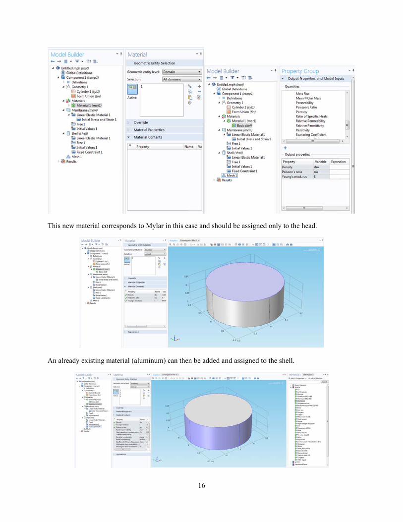
This new

An alread

material corr

dy existing ma

responds to M

aterial (alumin

Mylar in this c

num) can then

16

ase and shoul

n be added an

ld be assigned

nd assigned to

d only to the

o the shell.

head.

Note that model.

After matconditionsyour modthe modelassigned iThis is shElastic M‘Membran

since no Phy

terials are adds. If your syst

del is quite easl can be morein the followiown below. Naterial’. To fine’ and select

sics were assi

ded, the most tem has well sy. If the boune challenging ng way. First

Note that ‘Initix the edges, ating it, and th

igned to the ‘

difficult part defined bounndary conditito create. Fort, the head is gtial Stress anda ‘Fixed Cons

he desired edg

17

bottom’ head

can begin: dendary conditioons are somer the one-headgiven an initid Strain’ alreastraint’ (edge

ges must be se

d, it is as if thi

etermining anons, or you caewhat ambigud system, the al in-plain strady exist unde) must be addelected.

is surface doe

nd assigning ban easily deteruous (as will b

boundary conress and the eer ‘Membranded by right c

es not exist in

boundary rmine them, tbe discussed lnditions are

edges are fixedne’ and ‘Lineaclicking

n the

then later)

d. ar

In both camodel – mthis case, entire she

These bou‘Eigenfreq

The meshmesh.

ases, the entirmodeling the c‘Shell’ shoulll should be s

undary conditquency’.

h should then

e shell must bcoupling of shd be right-clic

selected.

tions are suffi

be built by se

be fixed (this hell and headcked and a ‘F

icient to cond

elected ‘Mesh

18

is not physicd leads to somFixed Constra

duct the first S

h’ and clicking

ally accurate,mewhat ambigaint’ (surface)

Study by selec

g ‘Build all’ a

, but is sufficiguous bounda) should be ad

cting ‘Add St

after choosing

ient for a basiary conditionsdded, then the

tudy’ and sele

g the desired

ic s). In e

ecting

The studygraphs su

The studyof interestprovides rhead mea

The additimodel difis not inclboundary importantboundary physics (i

As a side heads (incwas quite

Square A

This syste

A rectangsupport inof the cyli

The plate

The Physi

y can then be rch as the one

y actually gent in this case. relatively accsurements.

ional conditiofferent boundaluded here beconditions fo

t, but knowingconditions fo.e. ‘Membran

note, the twocluding air bededicated, th

Aluminum Pl

em was much

gular prism is n the experiminder is irrele

’s material wa

ics used for th

run by selectishown below

nerates plots foIf the physicaurate mode sh

ons and studieary conditioncause it is (m

or each systemg how to add or each differene’, ‘Shell’).

o-head systemetween the heahey could accu

ate

h easier to mod

added insteadental setup). T

evant, only the

as assigned to

he plate was ‘

ing the study w.

for both the shal constants ohapes at frequ

es seen on thes which shou

much) more com is completethem for youent ‘Physics’

m was attempteads) is enormurately model

del, but the ov

d of a cylindeThe exact geoe diameter ma

o aluminum.

‘Solid Mecha

19

and clicking

hell and membof Mylar and tuencies simila

e left side of tuld be more phomplicated, giely different –ur individual s

added, feel fr

ed and discarmously compli

l the entire sn

verall process

er, with a cyliometry of theatters.

anics’.

‘Compute’. T

brane, but onthe tension arar to those see

the some of thhysically accuives worse re

– the specific system is. Thefree to peruse

rded – the moicated. It is, hnare drum sys

s is similar.

indrical post ge plate and cyl

This will resu

nly those of thre set correctlen experimen

he pictures aburate. The des

esults in most conditions heere are a multthem by righ

odeling of the however, possstem using CO

going throughlinder were m

ult in various

he membrane ly, this modelntally in the o

bove are presescription of thcases, and th

ere are not titude of diffe

ht-clicking on

coupling betwsible. If someoOMSOL.

h the middle (modeled; the h

are l ne-

ent to hese

he

erent the

ween one

(the height

20

The boundary conditions are: the entire cylindrical support is fixed. The edges of the plate contacting the cylinder are fixed.

An eigenfrequency study was used.

The plots generated match (very) well with those seen experimentally by the other student in Spring 2014. An example is shown below from the eigenfrequency at 114 Hz. The geometry used is clear from the 3D image.

If interested, this entire model as well as the plots which match the experimentally studied eigenmodes can be found in the Physics 406 backup on the lab computers. This model is relatively easy to walk through, so it is a good place to get started if interested in COMSOL.

Side note: it is in fact unnecessary to model the cylindrical post, as long as the edges of the plate which would contact it are fixed. However, it is a nice visual aid to imagine the actual experiment.