Ris0—R—1181(EN)

Modal Analysis of Wind Turbine BladesGunner C. Larsen, Morten H. Hansen, Andreas Baumgart, Ingemar Carien

Ris0 National Laboratory, Roskilde, Denmark February 2002

Abstract Modal analysis has been used to identify natural frequencies, damp­ing characteristics and mode shapes of wind turbine blades.

Different experimental procedures have been considered and the most appropri­ate of these has been selected. Although the comparison is based on measurements on a LM19 m blade, the recommendations given are believed to be valid for other types of wind turbine blades as well.

The reliability of the selected experimental analysis has been quantified by es­timating the unsystematic variations in the experimental findings. Satisfactory results have been obtained for natural frequencies, damping characteristics and for the dominating deflection direction of the investigated mode shapes. For non­dominating deflection directions of the investigated mode shapes, however, the observed experimental uncertainty may be considerable - especially for the tor­sional deflection.

The experimental analysis of the LM19 m blade has been compared with results from a FE-modeling of the same blade. For some of the higher modes substantial discrepancies between the natural frequencies originating from the FE-modeling and the modal analysis, respectively, are observed. Comparing the mode shapes (normalized with respect to the tip deflection in the dominating deflection di­rection) good agreement has been demonstrated for the dominating deflection direction. For the non-dominating deflection directions, the qualitative features (i.e. the shape) of measured and computed modes shapes are in good agreement, whereas they quantitatively may display considerable deviations.

Finally, suggestions of potential future improvements of the experimental pro­cedure are discussed.

ISBN 87-550-2696-6ISBN 87-550-2697-4 (Internet)ISSN 0106-2840

Print: Pitney Bowes Management Services Denmark A/S, 2002

Contents

1 Introduction 5

2 Theory of modal analysis 72.1 Discrete blade motion 72.2 Extraction of modal properties 8

3 Experimental method 123.1 Modal analysis techniques 123.2 Experimental cognitions 133.3 Recommended experimental procedure3.4 Modal analysis 26

4 Results 304.1 Natural frequencies 304.2 Damping characteristics 304.3 Mode shapes 31

5 Conclusion 40

Acknowledgements 42

References 43

A Discrete blade motion 45

B Errors on mode shapes 47

C Optimum transfer function 51

D Uncertainty in spectral estimates 59

E Alternative experimental strategies 63

F Instrument specifications 69

G FEM Model 71

21

Ris0-R-1181(EN) 3

4 Ris0-R-1181(EN)

1 Introduction

As part of the certification procedure, all wind turbine blade prototypes are sub­jected to an experimental test procedure in order to ensure that the produced wind turbine blade fulfill the actual design requirements. In addition to experimental tests of load carrying capacity under extreme loading, and tests of the fatigue resistance, it is common practice to supplement with tests of the basic dynamic properties of the blades, such as natural frequencies and damping properties, as these are essential for the dynamic behaviour and structural integrity of the entire wind turbine. Usually, these dynamic characteristics are determined for the lowest 3-4 flexural bending modes and for the first torsional mode.

However, detailed knowledge to natural frequencies and structural damping characteristics does not by itself guarantee/ensure an optimal dynamic behaviour of the wind turbine when subjected to aerodynamic forces arising from the im­posed wind field. In resent years, stability problems in wind turbine structures have obtained increasing attention due to the trend towards larger and more flexi­ble structures. A well known example of a stability problem, that eventually might lead to failure of the whole structure, is the occurrence of dynamic unstable edge­wise vibrations. For aerodynamic loading in general1, and for dynamic stability problems in particular, the deflection patterns of the wind turbine blades are of vital importance. For a wind turbine blade, the deflections of interest are lateral translations (flapwise, edgewise) and cord rotation (about the blades longitudinal axis).

For reasons of simplicity it is common practice to model wind turbine com­ponents as beam structures in aeroelastic computations. Warping is usually ne­glected, justified by the fact that the main components are structures with closed cross sections, whereas the structural couplings between flexural bending in the two principal directions and structural couplings between torsion and flexural bending are usually included, as such structural couplings may significantly af­fect the aerodynamic load characteristics of a wind turbine blade. Although, in principle included in the traditional Euler or Timoshenko beam modeling of wind turbine blades, the correct specification of such structural couplings is a delicate matter.

For the verification of structural models, it is therefore of interest to extend the traditional dynamic test procedures with new experimental methods suitable for determination of structurally coupled mode shapes. The present report describes a test procedure that, in addition to determination of natural frequencies and structural damping characteristics, also provide such information.

Modal analysis is by far the most common method used to characterize the dynamics of mechanical systems, and it produces very illustrative and easy in­terpretable results. The selected experimental procedure is based on the impact modal testing technique.

The specific experimental procedure is designed as to (simultaneously) resolve flapwise translation, edgewise translation and cord rotation in a selected number of cross sections. These deformations are determined with respect to a predefined reference axis based on three measured translational accelerations in each cross section. The positions and directions of action of the three accelerometers are chosen appropriately.

An interest for internal blade structural mechanics, as well as for experimen­tal modal analysis, has existed since the early prototypes of large wind turbines.

-•-The aerodynamic loading (and damping) is intimately associated with the angle of attack of the incoming flow on the turbine blade - a fact that makes the structural coupling between blade flexture and torsion a matter of utmost importance.

Ris0-R-1181(EN) 5

The 38 m, filament-wound glass/epoxy blade, designed for the research prototype WTS-3 (Maglarp, Sweden), was subjected to an extensive dynamic test program before delivery. The blade was designed and manufactured by Hamilton Standard, and the tests were conducted in 1981. A ” full” experimental modal analysis was performed [7] using a hydraulic shaker (white noise, two directions at one blade station) and several accelerometers, measuring one edgewise and two flapwise ac- clerations, at each of about 20 blade stations. The evaluated frequency response functions were then subsequently compared with the corresponding results from a 3D shell element FE-model. The dynamic characteristics corresponding to the seven lowest natural frequencies were analysed.

Modal analysis has also been used to identify approximate mode shapes, asso­ciated with the the dominating deflection direction only (i.e. mode shapes exclud­ing structural coupling between torsion, flapwise and edgewise deformations), of medium size wind turbine blades (LM17 m and LM19 m) [8]. The approximate modes, related to the three lowest natural frequencies, were successfully identified based on the transfer function between a sinusoidal forcing applied in the blade tip and an accelerometer response recorded successively in up to 68 blade stations.

Compared to the previous work, the present experimental investigation aims at comparing different experimental modal analysis techniques and subsequently to identify the most appropriate of these considering expenses, time consumption, uncertainty and resolution.

The report is structured as follows: Chapter 2 gives the theoretical backgroundfor the modal analysis method. In Chapter 3 follows then a description of the ex­perimental considerations and cognitions, which are eventually summarized in a recommended experimental procedure. The results obtained, applying the recom­mended experimental procedure on a LM 19 m blade, are presented and discussed in Chapter 4. Finally, a conclusion on the findings from the study, together with recommendations for potential future refinements of the technique, are contained in Chapter 5.

6 Ris0-R-1181(EN)

2 Theory of modal analysis

This chapter deals with the theory of the modal analysis procedure used in the following experiments with wind turbine blades. The aim is to give an overview of this theory and to explain some of the experimental tasks related to the theory. Two different issues are discussed. First, the choice of three degrees of freedom in each cross-section to describe the motion of the blade. Second, the extraction of mode shapes, natural frequencies, and damping from measurements of transfer characteristics of the blade.

2.1 Discrete blade motionIn an experiment it is not possible to measure the motion of all material points of the wind turbine blade. Instead the motion is discretized. A finite number of degrees of freedom (DOFs) are used to describe the blade motion.

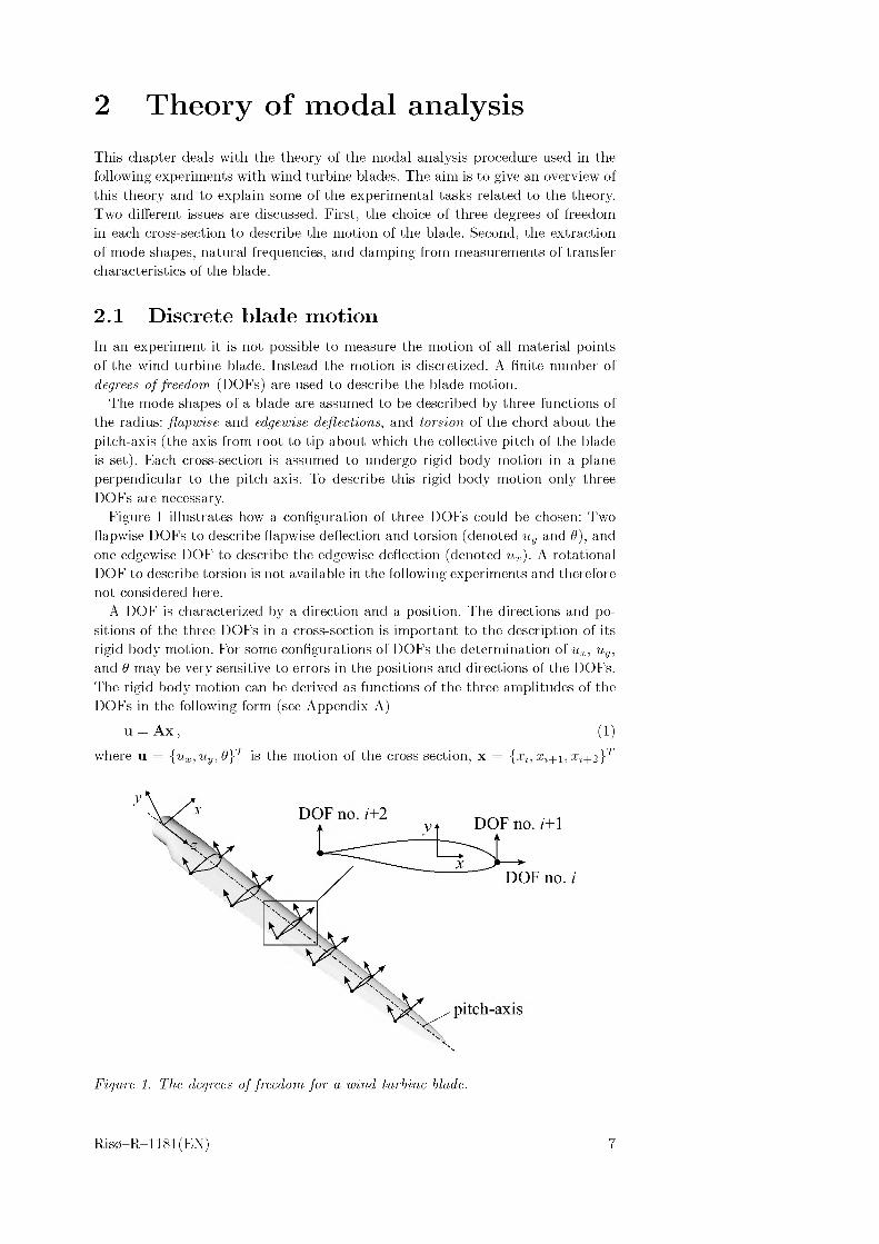
The mode shapes of a blade are assumed to be described by three functions of the radius: fl.apwise and edgewise deflections, and torsion of the chord about the pitch-axis (the axis from root to tip about which the collective pitch of the blade is set). Each cross-section is assumed to undergo rigid body motion in a plane perpendicular to the pitch-axis. To describe this rigid body motion only three DOFs are necessary.

Figure 1 illustrates how a configuration of three DOFs could be chosen: Two ftapwise DOFs to describe ftapwise deflection and torsion (denoted uy and 6), and one edgewise DOF to describe the edgewise deflection (denoted ux). A rotational DOF to describe torsion is not available in the following experiments and therefore not considered here.

A DOF is characterized by a direction and a position. The directions and po­sitions of the three DOFs in a cross-section is important to the description of its rigid body motion. For some configurations of DOFs the determination of uXl uy, and 0 may be very sensitive to errors in the positions and directions of the DOFs. The rigid body motion can be derived as functions of the three amplitudes of the DOFs in the following form (see Appendix A)

u = Ax , (1)where u = \uu,. 0\1 is the motion of the cross-section, x = {xj,xi+ i,xi+o}T

DOF no. i+2 DOF no. z'+l

DOF no. i

pitch-axis

Figure 1. The degrees of freedom for a wind turbine blade.

Ris0-R-1181(EN) 7

is the corresponding amplitudes in the three DOFs of the cross-section, and A isa three by three matrix given by the positions and directions of the three DOFs. Relation (1) is derived for any configuration of DOFs by assuming that the rotation of the cross-section due to torsion is small (0 < 1).

When choosing a configuration of DOFs, it is necessary to ensure minimal sen­sitivities of the motion u with respect to errors. Small sensitivities to errors in the measured amplitudes x requires small elements of A. Small sensitivities to errors in the configuration of DOFs requires small derivatives of elements in A with re­spect to the positions and directions of the DOFs. More specific considerations regarding the proper choice of DOFs are given in Appendix A.

Using relation (1) a mode shape of the blade can be estimated in a number of cross-sections, presuming the corresponding modal amplitudes have been measured in the three DOFs of each cross-section. How to obtain these modal amplitudes from an experiment is the topic of the next section.

2.2 Extraction of modal propertiesThe extraction of modal properties used in the following experiment is based on a formulation of the blade dynamics in the frequency domain. A frequency domainformulation has some advantages which are useful in the modal analysis. This section contains some mathematics which explains these advantages, and which helps with the introduction of the experimental procedure and the modal analysis.

Modal properties from an eigenvalue problem

The natural frequencies and logarithmic decrements are the eigenvalues, and mode shapes are the eigenvectors of an eigenvalue problem. To introduce this mathe­matical concept the linear equation of free motion for the blade is considered. The motion of the blade is described by L DOFs as shown in Figure 1. The deflection in DOF i is denoted xi, and the vector x describes the discretized motion of the blade. Assuming small deflections and moderate rotation of the blade cross-sections, the linear equation of motion can be written as:

Mx + Cx + Sx = 0, (2)

where (') = d/dt, and the matrices M, C and S are the mass, damping and stiffness matrices. Inserting the solution x = v ext into equation (2) yields

(A2M + AC + S) v = 0, (3)

which is an eigenvalue problem. The solution to this problem is the eigenvalues Ak and the corresponding eigenvectors vk for k = 1, 2,...,L. The eigenvalues of a damped blade are complex Ak = ak + i^k. The relationships between natural frequencies fk, logarithmic decrements Sk and the eigenvalues are

fk = 2n^k and Sk = ^k/fk . (4)

Instead of logarithmic decrements Sk as a measure of damping, the term damping factors are sometimes used for the quantity ak. The eigenvector vk contain the modal amplitudes vk,i in all DOFs for mode number k. Using relation (1), the flapwise- and edgewise deflections, and the torsion of the mode shape can be computed for each cross-section from the modal amplitudes vkyi, vk,i+i, and vk}i+2.

The modal amplitudes for a damped blade are complex. The imaginary parts describe phase shifts between the motions at different points on the blade. For a lightly damped blade these phase shifts are small and are generally neglected. When the imaginary parts of the modal amplitudes are neglected the resulting

8 Ris0-R-1181(EN)

mode shapes are termed normal mode shapes, otherwise they are termed the com­plex mode shapes of a damped blade. Normal mode shapes are characterized by having fixed nodes whereas the nodes of complex mode shapes are traveling.

The above eigenvalue problem shows that the problem of determining natural frequencies, logarithmic decrements, and mode shapes of a blade could be solved if one had a way to measure the mass, damping, and stiffness matrices. Such mea­surements are however not possible. Instead one can measure transfer functions in the frequency domain which hold enough information to extract the modal properties.

Definition of transfer functions

A transfer function describes in the frequency domain what the response is in one DOF due to a unity forcing in another DOF. It is defined as:

Hj H = x (w)/F H, (5)

where w is the frequency of excitation, Xi(w) is the Fourier transform of the re­sponse xH (t) in DOF i, and Fj (w) is the Fourier transform of a force f (t) acting in DOF number j. By measuring the response xi and the forcing fj, and perform­ing the Fourier transformations, the transfer function Hij can be calculated from definition (5). This transfer function is one of L x L transfer functions which can be measured for the blade with L DOFs. The complete set of functions is referred to as the transfer matrix H.

From transfer functions to modal properties

An estimation of all mode shapes can be obtained from only one row or one column of the transfer matrix H. A row of transfer functions can be obtained from an experiment by measuring the response in all DOFs, while the point of excitation is fixed to one DOF. To obtain a column of H, the response is measured in one DOF while the point of excitation is moved between all DOFs. Either one of these procedures can be used to obtain all mode shapes.

To understand this basis principle of modal analysis consider the linear equation of motion (2) for the blade with external excitation

Mx + Cx+ Sx = f(t), (6)

where the vector f is a forcing vector containing the external forces fj (t) which may be acting in the DOFs j = 1, 2,...,L. To solve this equation, it is assumed for now that the eigenvectors vk are known. The orthogonality of eigenvectors yields that any solution to equation (6) can be written as the modal expansion

Lx(t)=^2 vk %(t), (7)

k = 1where qk are the time-dependent generalized coordinates. Inserting (7) into the equation of motion (6), multiplying by v^ from the left, and using the orthogo­nality of eigenvectors2, equations (6) reduces to

qk — 2&k qk + (wk + <?2) qk = vTf , k = 1, 2,...,L. (8)

This equation of motion shows that the generalized coordinates qk are uncoupled, i.e., the modes of the blade are uncoupled.

2 The eigenvectors satisfy the orthogonality conditions vfMv; = vf Cv; = vf Sv; = 0 for Xk = X;. With the normalization of the eigenvectors vf Mvk = 1, it can be shown that uf Cvk = -2ak and vf Svk = u>2 + . Note that the orthogonality condition does not apply in the case of multiple eigenvalues. In such case, special modal analysis techniques are needed for decoupling of modes.

Ris0-R-1181(EN) 9

The decoupling of modes yields that transfer functions can be written as asum of modal transfer functions. Using definition (5), and Fourier transforming expansion (7) and equations (8), the transfer matrix can be derived as

NH(w) = %] Hk(w)

k=1

NEr-------k=1 (iw - Ok - iWk

vkvT(iw — Ok + iwk)

(9)

This relation is the basis of modal analysis. It relates the measurable transfer functions to the modal properties wk, ok, and vk. Each mode k contributes with a modal transfer matrix Hk to the complete transfer matrix. Hence, a measured transfer function can be approximated by a sum of modal transfer functions:

NHij (w) ~ ^ y Hk,ij (w) ,

k=1(10)

where the modal transfer functions Hk,j (w) by decomposition can be written as

Hk,ij (w)rk,ij rk,ij

iw — pk iw — pk ’(11)

where the bar denotes the complex conjugate, pk = ok + iwk is called the pole of mode k, and rkj = vk,ivk,j is called the residue of mode k at DOF i with reference to DOF j. Thus, a pole is a complex quantity describing the natural frequency and damping of the mode. A residue is a complex quantity describing the product of two complex modal amplitudes. The modal properties are extracted from measured transfer functions by curve fitting functions derived from (10) and (11) with poles and residues as fitting parameters. There are different curve fitting techniques, however, a few basic concepts are common for all these techniques.

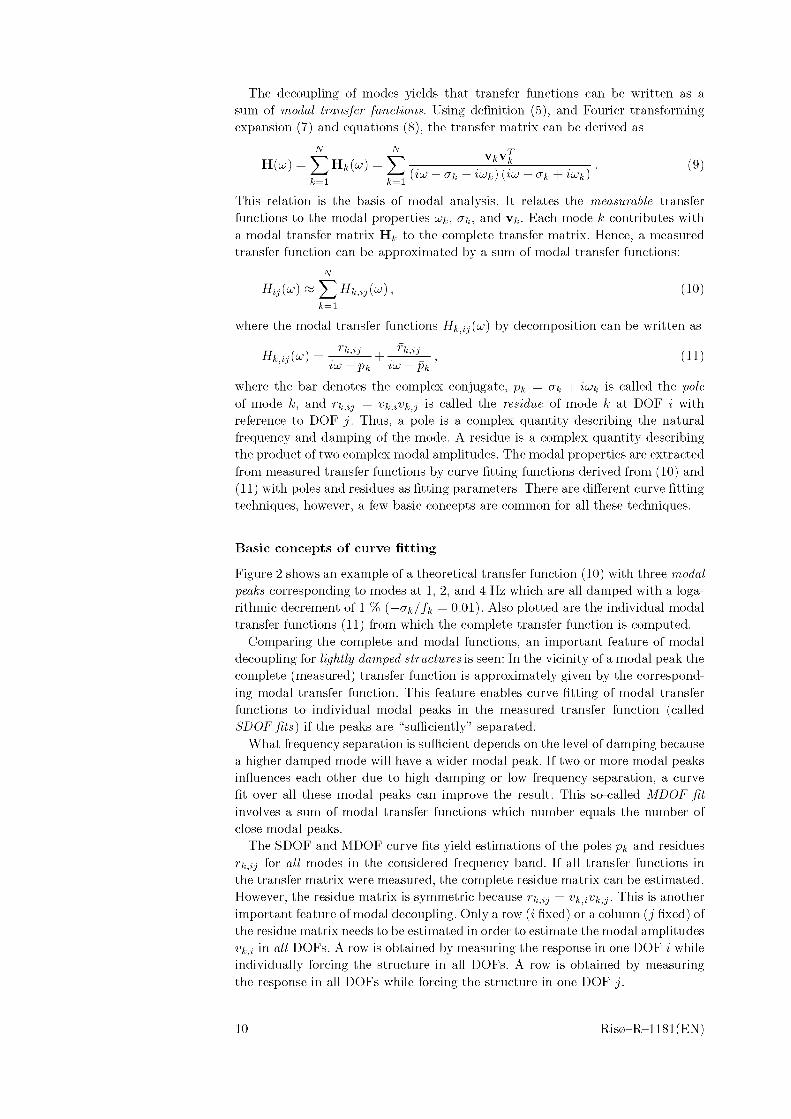
Basic concepts of curve fitting

Figure 2 shows an example of a theoretical transfer function (10) with three modal peaks corresponding to modes at 1, 2, and 4 Hz which are all damped with a loga­rithmic decrement of 1 % (— ok/fk =0.01). Also plotted are the individual modal transfer functions (11) from which the complete transfer function is computed.

Comparing the complete and modal functions, an important feature of modal decoupling for lightly damped structures is seen: In the vicinity of a modal peak the complete (measured) transfer function is approximately given by the correspond­ing modal transfer function. This feature enables curve fitting of modal transfer functions to individual modal peaks in the measured transfer function (called SDOF fits) if the peaks are “sufficiently” separated.

What frequency separation is sufficient depends on the level of damping because a higher damped mode will have a wider modal peak. If two or more modal peaks influences each other due to high damping or low frequency separation, a curve fit over all these modal peaks can improve the result. This so-called MDOF fit involves a sum of modal transfer functions which number equals the number of close modal peaks.

The SDOF and MDOF curve fits yield estimations of the poles pk and residues rkj for all modes in the considered frequency band. If all transfer functions in the transfer matrix were measured, the complete residue matrix can be estimated. However, the residue matrix is symmetric because rkj = vk,ivk,j. This is another important feature of modal decoupling. Only a row (i fixed) or a column (j fixed) of the residue matrix needs to be estimated in order to estimate the modal amplitudes vk,i in all DOFs. A row is obtained by measuring the response in one DOF i while individually forcing the structure in all DOFs. A row is obtained by measuring the response in all DOFs while forcing the structure in one DOF j.

10 Ris0-R-1181(EN)

Complete transfer fen. Hzy Mode 1, Hltj Mode 2, H2ij Mode 3, H3 i7

Frequency [Hz]

Mgwre ^larnp/e o/ ZAe modal decowpllrng a traMs/er /brnctloM.

Another basic concept of curve fitting in modal analysis is the use of local and global curve fits. Note that the denominator of the modal transfer functions (11) are independent of the index i and j. This means that the poles of a row or column of transfer functions are identical for each mode. A global curve fit uses this feature by first estimating the poles of each mode from all transfer functions. In the second step the residues in each DOF of each mode are estimated from individual curve fits to each transfer function using that the poles are given from the first step. This procedure decreases the error on the poles and residues compared to a local curve fit where the both poles and residues are estimated by individual SDOF or MDOF fits to each transfer function.

These concepts of SDOF/MDOF and local/global curve fits are general methods in modal analysis. The actual curve fitting routines will be discussed in Section 3.4 dealing with the modal analysis of measured transfer functions.

Accuracy of the estimated modal properties

The accuracy of the estimated natural frequencies, damping, and mode shapes depends basically on three things: Accuracy of the measured transfer functions, linearity of the blade dynamics, and accuracy of the DOF characteristics.

Measurement errors on the transfer functions directly influences the curve fits which are used to estimate the modal properties. Measurement errors can have many sources in experimental modal analysis. Some of them can be cause by external mechanical noise, internal electrical noise, false calibration of transducers, etc.. Also insufficient frequency resolution of the transfer functions decreases the accuracy of the curve fits.

The non-linearities in the blade dynamics will distort the transfer functions yielding that the theoretical basis for the curve fits may become invalid. Such non-linearities could arise from large deflections of the blade, or for example from a loose tip brake that slides in its support during the measurements.

Even though the modal amplitudes are estimated with high accuracy, the esti­mated mode shapes may be inaccurate due to poor measurement of the directions and positions of the DOFs.

All these sources of error are considered in the experiment procedure presented in the next chapter. Methods to estimate the accuracy of the natural frequencies, damping, and mode shapes are also discussed.

Ris0-R-1181(EN) 11

3 Experimental method

The present chapter deals with considerations related to the practical implemen­tation of the modal analysis procedure (as described in the previous chapter) in dynamic testing of wind turbine blades. First different possible experimental strategies are discussed, then the experiences gained from the performed experi­mental program are outlined which subsequently leads to formulation of a recom­mended practice, and finally the extraction of the modal characteristics from the measured quantities are described.

3.1 Modal analysis techniquesModal analysis provides information on the dynamic characteristics of structural elements at resonances, and thus aids in understanding of the detailed dynamic behaviour of these. A basic feature with the technique is the presumption of lin­earity of the mechanical system, as described in Chapter 2. A quantitative test on linearity can be performed, based on a measured complex frequency response func­tion (resulting from a sinusoidal excitation), by applying the Hilbert Transform as described in [5]. Other indications of possible non-linearities may be obtained from evaluation of suitable coherence functions as is described in more details in the following.

Having decided to base the experimental testing of wind turbine blade dynamics on modal analysis, two basic questions arises: 1) how to excite the wind turbine blade, and 2) how to ensure acceleration responses that can resolve the requiredtypes of deflection patterns in selected cross-sections.

Excitation techniques

The different excitation techniques fall in two basic classes - transient excitation (free vibration) and continuous excitation (forced vibration).

Continuous excitation is typically performed with electromagnetic or hydraulic based exciters able to produce f. ex. swept-sine excitation, white noise excitation, pseudo-random excitation or periodic-random excitation. Usually, the excitation is subjected in only one point, however, for large or highly damped structures it might be advantageous to apply more exciters simultaneously.

The transient type of excitation is usually associated with either an impulse force loading or an instantaneous release from an initial deflection of the structure (known as the snap back principle).

Required recordings

Independent of the selected excitation method, it is in practice usually necessary to treat the selected blade cross-sections successively, in order to obtain a suit­able spatial resolution of the eigenvectors describing the mode shapes for a large structure as a wind turbine blade. However, in principle, if unlimited resources were available for equipment, all the required response signals could be measured simultaneously.

In its simplest form, a modal analysis requires recordings only of the structural response. In this situation a reference response signal is required to relate suc­cessively recorded cross-sectional responses mutually and thereby determine the resonance deformation pattern. However, applying this experimental procedure excludes the results from being subsequently used in a system analysis providing (absolute) information on the structure stiffness and mass properties. The crucial

12 Ris0-R-1181(EN)

point is here, that only information on the relative proportion between stiffness-and mass properties is obtained.

If, in addition to the structural response, also the force excitation (magnitude and direction) is recorded, then the system parameters (stiffness- and mass prop­erties) can be identified in addition to information on natural frequencies and deflection/damping properties at resonances.

Analysis methods

The analysis method, used to extract the required results from the measured data, can be performed either in the time domain or in the frequency domain. The time domain method is based on a least square optimization of modal ampli­tudes, modal damping and modal phases, given a selected (but arbitrary) number of resonances. The frequency domain analysis is based on the concept of trans­fer functions as described in Chapter 2 (when the excitation force is recorded - otherwise it is based on the spectral energy contained in the resonance peaks).

Investigated experimental procedures

In the present experimental campaign, the main effort has been put on a tradi­tional approach applying transient force excitation in combination with frequency domain analysis based on transfer functions. The motivation for this choice is elaborated on in Appendix E. The experiences gained from the impact excitation approach, during the experimental campaign, are reported in Section 3.2 which directly leads to a detailed description of a recommended experimental practice in Section 3.3 and an associated analysis method in Section 3.4. Alternative ex­perimental strategies and analysis methods, investigated during the course of the project, are briefly described in Appendix E.

3.2 Experimental cognitionsAll the experimental tests have been performed on a LM 19.1 m wind turbine blade mounted in a horizontal position by clamping the root blade flange to a rigid test stand. The blade is not a standard product, but a LM19 version with increased edgewise structural damping characteristics (cf. the logarithmic decre­ments presented in Section 4.2). In order to avoid large initial deformations, that could potentially complicate the practical determination of a suitable geometric reference axis, and in addition to obtain a realistic static load picture for a blade mounted on a real wind turbine, the investigated blade structure has been mounted with the tip chord in a vertical position. Further, to prepare for a possible appli­cation of ’’skew” exciting forces (forces with an angle of the magnitude of 45 deg with the chord that is able to excite flapwise as well as edgewise dominated blade modes simultaneously) the blade is, for practical reasons, mounted with the robust leading edge (free of edges contrary to the tailing edge) pointing downwards.

Excitation

The transient force excitation is established by means of a hammer device of sufficient mass and velocity that impacts the turbine blade once, giving it an initial velocity and acceleration 3. The structure is at rest before the excitation. After the hammer impact, the (external) force is zero again, and in this situation

3Note, that the force excitation should be applied only at locations that is not nodes of relevant mode shapes.

Ris0-R-1181(EN) 13

equation (6) reduces to an initial value problem with only homogeneous solutions. The turbine blade thus oscillates with a superposition of its discrete eigensolutions.

Ideally, considering the excitation force mathematically to be described by a Dirac function, S(-), the hammer excitation enables all frequencies to be excited simultaneously with an equal amount of energy (a flat input spectrum). With the notation introduced in Chapter 2, this can be seen from

f (t) = foS(t - to), (12)

whereby the Fourier transform of the external forcing is formulated as

FH = fo . (13)

In practice, however, the concept of a Dirac function is only a (useful) theoretical abstraction, and the hammer hit will have a final duration in time, with the consequence that an upper cut-off frequency is introduced in the Fourier spectrum of the excitation force. This fact is utilized actively in the present experimental procedure, by applying the hammer head as a mechanical filter, and thus making the appropriate choice of the hammer head an important parameter for this type of transient excitation.

For wind turbine blades only a limited frequency band is of relevance - typically the frequency range between 0.5 Hz and 30 Hz. In this situation the hammer head can be tuned/tailored to concentrate the total excitation energy, supplied by the hammer hit, in this frequency band. Introduction of a cut-off frequency in the excitation spectrum in this way has appropriate implications for the required signa— and sampling4 resolution.

The implications for the signal resolution are closely related to the signal/noise ratio associated with the relevant frequency range. If undesirable high frequencymodes were excited, high signal levels of accelerations in a frequency band, that are without practical relevance, would be present in the response signal. As the magnitude of the acceleration response equals the deflection amplitude weighted with the associated natural frequency squared (harmonic oscillation), the sensi­tivity of the amplifiers would have to be adjusted to these short-term peeks, thus giving rise to unacceptable amplitude resolution of the important low-frequency part of the response. This would in turn reduce the signal/noise ratio in the rele­vant frequency range. By introducing the mechanical filter these short-term peaks are avoided, and, in addition, the magnitudes of the excitation- as well as of the response signal, in the important frequency range, are enhanced. Assuming the share of the noise, originating from the electronic measuring equipment, to be the dominant noise contribution, and further assuming this contribution to be inde­pendent of the signal level, the signal/noise ratio will be improved, in the relevant frequency range, as a consequence of application of the mechanical filter.

The implications for the sampling resolution are related to a possible distortion of FFT generated spectra caused by aliasing [11]. As we aim at performing the signal analysis in the frequency domain, it is of vital importance to ensure a correct representation of the FFT transformed excitation- and response signals. By introducing an appropriate mechanical filter, aliasing is avoided by selecting a sampling rate with a Nyquist frequency, that exceeds the introduced filter cut-off frequency.

The cut-off frequency, introduced by the mechanical filter, is closely related to the duration of the contact between blade and hammer head in a stroke. The contact duration in turn depends on impact velocity, rebound velocity, elastic(and plastic) properties of the structure/hammer, tip radius and hammer mass.

4Time resolution of the excitation signal as well as of the response signal.

14 Ris0-R-1181(EN)

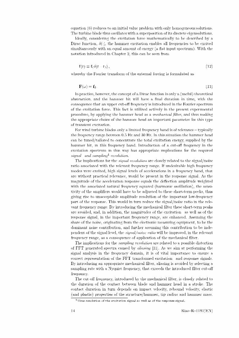
Figure 3 illustrates the fundamental effect on the excitation force characteristics caused by applying two different stiffnesses of the hammer head. The results are based on a simple mathematical model, in which the LM 19 m blade is represented by a beam model with 9 degrees of freedom. No damping of the structure is taken into account in the modelling.

Even though the general hammer motion is approximately the same for both ex­periments (and thus the momentum exchanged) there are significant differences. The impact duration is significantly longer using the soft hammer head, corre­sponding to the fall off in the spectrum of the excitation force and the reduced content of high frequency component in the response.

Depending on the dynamic characteristics of the blade, the hammer head that suits the actual experiment best must be selected. This is basically a trial and error process that may be facilitated/supported by experience and by numerical investigations. Note, that the choice of a suitable hammer head will usually (in addition to the general dynamic characteristics of the blade) also depend on the particular cross-section to be investigated.

Response

The response signals consist of accelerations measured in an arbitrary number of cross-sections along the pitch axis. Each cross section is instrumented with two (spatially displaced) uniaxial accelerometers recording the accelerations in the flapwise direction, and one uniaxial accelerometer recording the acceleration in the edgewise direction, respectively. As described in Section 2.1, each cross section is assumed to deflect as a rigid body (in a plane perpendicular to the

soft tip

hammer deflection

Figure 3. Numerical model of hammer excitation of the blade applying two different stiffnesses of the hammer head.

Ris0-R-1181(EN) 15

pitch axis). With this assumption, supplemented by an assumption of small de­flections, a unique relationship exists between the accelerometer recordings and the modal displacements of the cross-section expressed in terms of flapwise de­flection, edgewise deflection and torsion around the pitch axis, respectively. This relationship can be utilized in sensitivity considerations aiming at determining the most suitable definition of the DOF’s within a cross-section. Using resolution of the torsional deflection (which appears to the most critical of the investigated deflection types) as the decisive factor, two simple guidelines can be derived (cf. Appendix B):

• The distance between the two accelerometers recording the flapwise acceler­ations should be as large as (practical) possible; and

• The angle between their measuring axis should be as close as possible to zero degrees.

Reference axis

In order to link measured modal deflections in one cross-section to modal deflec­tions in other cross-sections, a reference axis for the blade must be defined. The reference axis ensures that the deflections computed for each cross-section, ac­cording to the algorithm described in Appendix A, all refer to the same Cartesian co-ordinate system. In the present experimental campaigns, the reference axis has conveniently been chosen as the symmetry axis from the cylindrical blade root cross-sections extended to the blade tip. The practical aspects related to estab­lishment of the reference axis are further described in Section 3.3.

Error sources

When resting on impact testing and extracting the modal characteristics in thefrequency domain, measurement of the transfer function, as defined in Section 2.2, become of vital importance (cf. Section 3.4). Consequently, besides the accuracy of geometric quantities, such as measuring/excitation location and direction, the accuracy of the measured transfer function, reflecting the accuracy of the sensors and the recording system, is important. These two classes of error sources are addressed in the following.

Uncertainties in DOF characteristics

To reduce the uncertainties, originating from erroneous definition of the geom­etry (i.e. bad specification of forcing/recording location or direction), different approaches have been considered.

Two approaches has been examined for the alignment of the response recording: 1) mounting of the accelerometers directly on the surface of the wind turbine blade, and 2) mounting of the accelerometers on a special designed support structure attached to the blade.

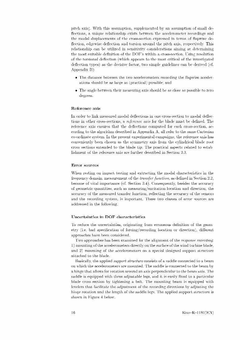
Basically, the applied support structure consists of a saddle connected to a beam on which the accelerometers are mounted. The saddle is connected to the beam by a hinge that allows for rotation around an axis perpendicular to the beam axis. The saddle is equipped with three adjustable legs, and it is easily fixed to a particular blade cross-section by tightening a belt. The mounting beam is equipped with levelers that facilitate the adjustment of the recording directions by adjusting the hinge rotation and the length of the saddle legs. The applied support structure is shown in Figure 4 below.

16 Ris0-R-1181(EN)

Figure /or response mea8!/remeM(8.

Concerning determination of the DOF locations, relative to some global blade coordinate system, the two recording methods are considered to result in uncer­tainties of the same order. However, the determination of the DOF locations is somewhat simpler with the accelerometers attached directly to the blade surface, where it suffices to measure simple relative coordinates (e.g. relative to blade root, leading edge, trailing edge etc.), and then subsequent transform these to the abso­lute coordinates, based a detailed drawing of the actual blade. The complicating factor, when using the support structure, is that the position of the support struc­ture, relative to a cross-section, can not be easily measured. This problem can, however, be solved by aligning a reference laser beam along the blade at a conve­nient distance from the blade surface (cf. Section 3.3). Aligning the accelerometers in the vertical direction, the point of intersection, between the laser beam and a screen mounted on the support structure, provides the necessary information for assessing the DOF positions in the global coordinate system.

Concerning determination of the DOF directions, the recording method, based on the support structure, is superior, as it turned out to be difficult to control the measuring directions of the accelerometers, when these were mounted directly on the blade surface. An error introduced in the measurement direction in turn introduces a considerable error in primary the blade torsion deflection component (c.f Appendix B). For this reason, it was decided to base the final blade testing on the recording approach based the measurement bridge, where much better resolution of the torsion response was obtained.

The sensitivity of the (torsional) mode shapes, on errors in location and di­rections of DOF’s, can be reduced by appropriate definitions of the DOF’s. In Appendix B it has been shown that an optimal DOF configuration (assuming three DOF’s in each blade measurement section) requires the distance between the two flap wise DOF’s to be as large as possible, and the directions of these to be identical.

Analogous to misalignment of the recording equipment, errors are introduced in the blade mode deflections, if the specified direction of the applied forcing is contaminated with uncertainties. In order to avoid (minimize) such errors, three different techniques for generation of impact loading were examined: a pendulum, a hand-actuated hammer, and a special guided hammer (the ”seesaw” - depicted in Figure 6).

The pendulum used here was a piece of heavy spar, mounted and supported

Ris0-R-1181(EN) 17

through a chain attached to each end. This pendulum is characterized by rather good control of force level and direction, but it takes a very stable support struc­ture to carry it (e.g. an industrial truck), and the use is restricted to horizontal excitation. For these reasons this type of hammer exciter was excluded in the further analyses.

The classical hand-actuated hammer was used only for exciting a small test blade. Due to the difficulties controlling the direction as well as the force level,this method was found unattractive.

The ”seesaw” was in this case a welded, sledge-like piece of steel, carried and suspended by a standard workshop lift. This hammer is characterized by a good control of the force direction, however, with some difficulties in controlling the force level since this hammer is operated manually. It could be conveniently moved to different positions along the blade, to be operated for excitation in horizontal- as well as in vertical direction. In conclusion, this hammer was considered as the most appropriate for transient excitation of the wind turbine blade.

In addition to errors in the specified direction of the forcing and recording, possible errors in the specified location of these quantities also affect the result of a modal analysis. It is therefore essential that the measuring- and forcing locations are carefully determined.

Uncertainties related to the measured transfer function

The basic requirements for establishing the transfer function are that the input- and response signals are Fourier transformable, and that the input signal is non­zero at all frequencies of interest. These requirements are easily fulfilled. The next consideration is how to compute the transfer function. The straight forward method is of course to compute the transfer function directly as the ratio between the Fourier transforms of the response and input, as expressed in the definition given in equation (5).

However, due to the inevitable presence of extraneous noise in the measuredsignals, this procedure will result in estimates of the transfer function encumbered with significant statistical uncertainty being partly based on only single (raw) estimates of the Fourier transforms of the noise contributions. A more suitable approach, involving a signal averaging procedure, is to determine the transfer function as the ratio between the cross-spectrum (between the observed input- and the observed response signal) and the power spectrum of the observed force signal. It can be shown that this choice of transfer function estimate, for signals containing external noise contributions, is an optimum choice in the sense that the estimate, in an average sense, is the best possible (cf. Appendix C).

We now interpretate the observed force signal, as well as the observed response signal, as superpositions of a physical signal and an inevitable noise contribution. Assuming that the noise, superimposed on the physical response signal, is uncor­related with the physical input signal, and that the noise, superimposed on the physical input signal, is uncorrelated with the physical input signal as well as with the ideal response signal, the optimum transfer function estimate, Hij(w), is determined from (cf. Appendix C):

Hij(w)1 + Sgr(w)

(14)

where Hij (w) is the transfer function associated with the physical force- and response signals, SF X (w) is the cross-spectrum between the observed forcing and the observed response, SjFt (w) is the power spectrum of the observed forcing,

18 Ris0-R-1181(EN)

SFjF(w) is the power spectrum of the physical forcing, and (w) is the powerspectrum of the noise superimposed on the force signal. The lower indices, i and j, indicate that the quantities are related to an experiment where the forcing is acting in DOF number j, and the response is measured in DOF number i.

Compared to a ” traditional” estimate of the transfer function, computed accord­ing to the definition given in equation (5), the present optimum transfer function estimate excludes the influence from the inevitable noise in the response signal. The price we payed, to avoid the influence from the response noise, is that the optimum transfer function estimate is a biased estimate of the ideal transfer func­tion. Equation (14) shows that the bias depends on the input signal/noise ratio only, and it tends consistently to zero when the input noise contribution approach zero.

In addition to the bias on the estimated transfer function, caused by natural variability of the input signal noise, the estimated transfer function is also affected by statistical uncertainty in the estimates of the (expected) cross- and autospectra. The statistical uncertainty on the spectral estimates is inversely proportional to the number of averages used in the estimate (cf. Appendix D), and usually quite few averages suffice (say, of the order of 5).

Finally, possible non-linearities in the investigated physical system will intro­duce variability in the estimated transfer function. The application of a transfer function in modal analysis presumes a linear constant parameter physical sys­tem, and in case this presumption is violated, the effect on the estimated transfer function will be similar to the effect caused by conventional signal noise. Possible non-linearities related to a wind turbine blade could be sliding between tip brake and the remaining part of the blade, non-linear damping characteristics or load- sensitive stiffness (unlikely for the load levels applied in the present experiments). Possible non-linearities (or errors), associated with the recording technique, could occur if the used measuring bridge is not completely fixed to the blade structure.

Error measures

A handy measure of the quality of the estimated transfer function (and thus the associated measurements) is the coherence function (cf. Appendix C). Having estimated the transfer function in terms of spectral quantities, as described above in equation (14), the coherence function is easily derived. The coherence function between the observed input- and the observed response signals, yjX (w), is defined as :

rX2ij (w)Sj'X (w)

SX X (w)Sj 'F' (w)

2

(15)

where SiXj X (w) is the power spectrum of the observed response signal.For perfect correlation (under a linearity assumption) between observed input-

and response signals, the coherence function can be shown to equal one5 (cf. Appendix C). The coherence function thus indicates the amount of noise and non-linear effects present in the investigated system. In addition, it indicates the amount of statistical uncertainty in the spectral estimates, on which the estimate of the transfer function is based. The coherence function is consequently perfectly suited as an ’’on-line” decision tool6 for assessing the number of averages required for obtaining satisfactory spectral estimates.

5 Except at resonance and antiresonance frequencies.6 The idea is to follow the convergence of the coherence function as function of the number of

applied averages.

Ris0-R-1181(EN) 19

Measuring the degree of correlation between the observed input- and responsesignals, the coherence function is intimately related to the quality of the estimated transfer function. It is therefore to be expected that the statistical error on the transfer function estimate depends on the coherence function. This error, as ex­pressed in terms of the standard deviation on the estimated transfer function,a^ (w), can be quantified explicitly as [9]

Hpt \rt 2 1/2

(16)

where N denotes the number of samples to be averaged in the estimate of the transfer function. In accordance with the above considerations, a^ (w) is seen todepend strongly on the coherence function. Also consistent with our expectations is that the standard deviation on the estimated transfer function is seen to tend to zero for N approaching infinity, or for the coherence function approaching one (cor­responding to a perfectly linear system without extraneous noise contributions). Note, that scatter on the transfer function in general might depend somewhat on the frequency.

Noise sources

As stated above, signal conditioning is an important parameter for achieving a satisfactory estimate of the system transfer function. One of the crucial recog­nitions, with the present type of blade tests, is that the response signal often combines low signal levels with low frequencies. This puts severe requirements on the response sensors. The experimental campaign has shown that the initially used B&K Delta Tron accelerometers (cf. Appendix F) performed unsatisfactory, and these were consequently replaced by conventional accelerometer types with an associated charge amplifier (cf. the setup described in Section 3.3).

However, the signal/noise ratio does not only relate to the electronic features of the recording equipment. Part of the noise in impact testing is due to multiple rebounds which vary randomly between tests. Reduction of such error sources depends on the skills of the experimenter, and the possibility for on-line filtering by continuously monitoring of the quality of the excitation. Analyses [2] have shown, that provided the force excitation do not vary between tests, the signal/noise ratio obtained from impact testing is comparable with the one obtained using harmonic excitation.

Roving recording or roving forcing

Due to the symmetry of the FRF matrix, expressing the dynamic relationship between excitation (direction, magnitude) at a given location and the structural response in one of the defined DOF’s, the experiment can be performed either with fixed excitation location and roving response recording, corresponding to the chosen discretization of the blade motion (cf. Chapter 2), or vice versa. Note, that in case of roving excitation, the mechanical filter, to be used, usually will depend on the position of the point of excitation. From a theoretical point of view no recommendations can be derived. However, practical aspects related to conduction of the experiments may decide which strategy is the most convenient. In case of hammer impact with the recording equipment mounted on measuring bridges, the experimental work involved in the execution of the two strategies is very similar. A small investigation of the coherence functions related to excitations/recordings in three cross-sections (positioned in the blade root, the middle of the blade, and at

20 Ris0-R-1181(EN)

the blade tip, respectively) was slightly in favour of the roving recording concept, as the best coherences were obtained in the outlier part of the blade using this concept.

Misinterpretation of results

It should be noted, that even in case all the above sketched technical requirements for minimization of possible error sources are meet, one might end up with a misleading interpretation of the achieved results, if the analysed physical system diverts /rom tke "Weed" pAysim/ system.

In the case of blade testing, such misinterpretations could occur if f. ex. the test stand does not have sufficiently stiffness, or if the measuring bridge is not properly designed, such that undesirable flexibilities from the bridge is introduced into the (compound) structural system7(or, alternatively, if the used measuring bridge is not completely fixed to the blade structure).

In the following section the experience gained through the measuring campaign, and briefly described above, is summarized in a recommended experimental prac­tice for wind turbine blade testing.

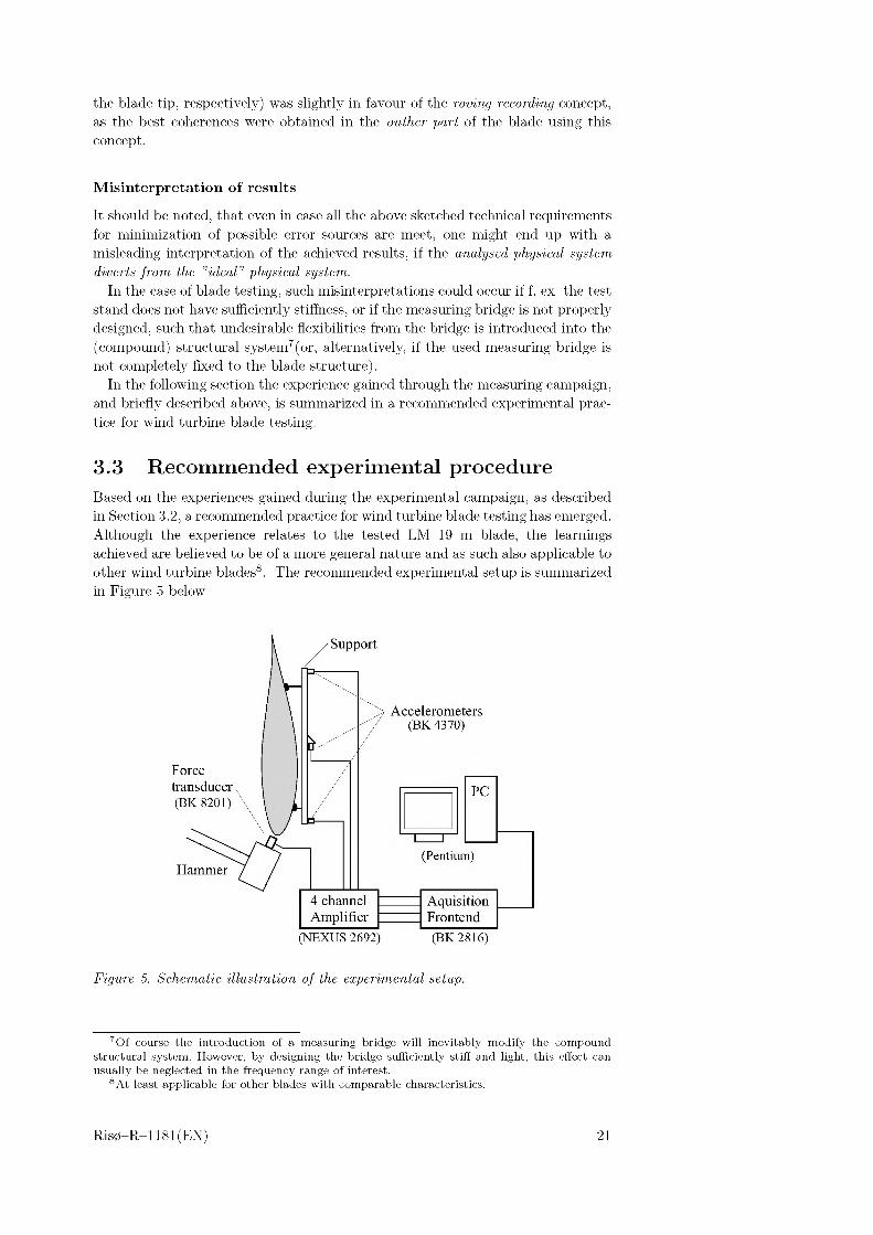
3.3 Recommended experimental procedureBased on the experiences gained during the experimental campaign, as described in Section 3.2, a recommended practice for wind turbine blade testing has emerged. Although the experience relates to the tested LM 19 m blade, the learnings achieved are believed to be of a more general nature and as such also applicable to other wind turbine blades8. The recommended experimental setup is summarized in Figure 5 below.

Support

Accelerometers (BK 4370)

Force transducer (BK 8201)

(Pentium)Hammer

AquisitionFrontend

4 channel Amplifier

(NEXUS 2692) (BK2816)

Figure 5. Schematic illustration of the experimental setup.

7 Of course the introduction of a measuring bridge will inevitably modify the compound structural system. However, by designing the bridge sufficiently stiff and light, this effect can usually be neglected in the frequency range of interest.

8At least applicable for other blades with comparable characteristics.

Ris0-R-1181(EN) 21

Mounting of the blade in a test stand

The blade is mounted in a horizontal position with the root flange clamped to a rigid test stand. To ensure that the correct physical system is investigated (i.e. the boundary conditions of the physical blade is as theoretically specified), it is important either to ensure that the test stand is perfectly rigid or, alternatively, to measure the flexibility of the stand. As motivated in Section 3.2, the blade is mounted with the tip chord in a vertical position and with the leading edge pointing downwards.

Transient loading

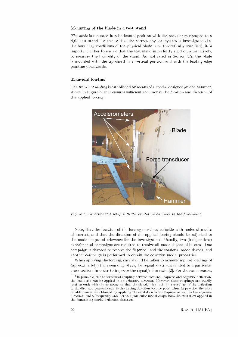
The transient loading is established by means of a special designed guided hammer, shown in Figure 6, that ensures sufficient accuracy in the location and direction of the applied forcing.

Figure 6. Experimental setup with the excitation hammer in the foreground.

Note, that the location of the forcing must not coincide with nodes of modes of interest, and that the direction of the applied forcing should be adjusted to the mode shapes of relevance for the investigation9. Usually, two (independent) experimental campaigns are required to resolve all mode shapes of interest. One campaign is devoted to resolve the flapwise- and the torsional mode shapes, and another campaign is performed to obtain the edgewise modal properties.

When applying the forcing, care should be taken to achieve impulse loadings of (approximately) the same magnitude, for repeated strokes related to a particular cross-section, in order to improve the signal/noise ratio [2], For the same reason,

9 In principle, due to structural coupling between torsional, flapwise and edgewise deflection, the excitation can be applied in an arbitrary direction. However, these couplings are usually relative week with the consequence that the signal/noise ratio for recordings of the deflection in the direction perpendicular to the forcing direction become poor. Thus, in practice, the most reliable results are obtained by applying the excitation in the flapwise as well as the edgewise direction, and subsequently only derive a particular modal shape from the excitation applied in the dominating modal deflection direction.

22 Ris0-R-1181(EN)

care should also be taken to obtain loadings of a suitable magnitude. In order not to lose the time advantage of the impulse technique, compared to other excitation methods, only a few repeated strokes are usually performed (in the present ex­perimental campaign between 3 and 5). Therefore, in addition to averaging, time sample windows are used to further improve the signal/noise ratio.

However, the selection of a suitable time window is not straight forward. To minimize the distortion of the frequency domain representation of the forcing, caused by applying a time sample window, requires minimization of the width of the main lope of the window transform. However, reducing the width of the main lope of the window transform implies decrease in the effect of the noise reduction obtained, as both the width of the main lope and the amount of noise reduction are inversely proportional to the width of the window in the time domain [2]. A well performing compromise is usually achieved by applying a time sample window with unity amplitude for the duration of the pulse combined with a cosine taper with a duration of 1/16 of the total sampling period decreasing from unity to zero.

Multiple rebounds should be avoided as the resulting load frequency spectrum will have zeros due to the periodic nature of such input signals. As a consequence, very low levels of force will be imposed at certain frequencies, giving rise to a poor signal/noise ratio at these frequencies. In practice, the applied hammer was equipped with a counteracting spring that facilitated a single-loop force history, by providing a favourable ratio between the hammer velocity and the hammer force counter acting the hammer movement just before impact. It is advised to quantify the quality of the imposed loading by on-line recording of the coherence function. In case of badly conditioned signals, the associated result should be rejected.

Imposing the loading as described above is a delicate matter, and it may well require some practice to achieve the necessary skills.

The hammer loading is recorded by means of a B&K force transducer type 8201 (cf. Appendix F) mounted on the hammer head, and with a mechanical ’’rubber filter” mounted on top (cf. Section 3.2). The characteristics of the mechanical filter (the hammer head hardness) must be adjusted based on a trial and error procedure, until the wanted input frequency characteristics (i.e. duration of the applied force excitation pulse) is achieved. In order to assure a suitable level of the forcing, over the frequency range of interest, the first zero crossing of Fourier transform of the loading must be well above the maximum natural frequency of interest. The optimum hammer head hardness will usually depend on the blade position, at which the impulse forcing is applied, due to the varying elastic stiffness of the blade structure with the position. The signal from the force transducer is, through a B&K 2635 charge amplifier, led to the B&K PULSE system.

Data aquisition system

In the present configuration, the PULSE system basically consists of the B&K Multichannel Aquisition front-end unit (Type 2816) integrated with the PULSE software (B&K Noise and Vibration Analysis Type 7700) running on a pentium Personal Computer equipped with two dedicated DSP bords (Type ZD 0812) that perform the realtime FFT and control the communication between the front- end and the PC. The setup is illustrated in Figure 5. The front-end unit was equipped with a B&K Signal Analyzer Interface Module (Type 7521), three 4- channel B&K Input Modules (Type 3022) and a B&K generator module (Type 3107). The Signal Analyzer Interface Module provides the sampling clock and transmits data to the TAXI interface. The Input Modules support measurements on four channels up to 25 kHz. The Generator Module is a single channel generator with a frequency range of 0 to 102.4 kHz (this module is only used to control of the random excitation using an electromagnetic exciter - cf. Appendix E). Further

Ris0-R-1181(EN) 23

details on the hardware can be found in Appendix F.

Spatial discretization

Depending on the mode shapes of relevance, a suitable spatial discretization alongthe blade axis is selected by focusing the response recordings on a limited number of blade cross-sections (cf. Section 2.1). In general, the selection of convenient measuring cross sections must take into account not to locate these at nodes of any of the relevant mode shapes. In the present experimental campaign a maximum of 20 cross sections were selected. For practical reasons, the cross section, at which the forcing is applied, has been selected not to coincide with any of the cross sections where response recordings are performed. The forcing is used as reference to link together the responses from the various cross-sections, and therefore a response recording at the cross-section where the force is applied is not required. Put in an other way, this means that the diagonal elements of the system transfer matrix, H, defined in Section 2.2 is not needed.

Recording of the response

For each cross-section three DOF’s are recorded - two aligned in the flapwise direction and one directed along the edgewise direction. The associated threeaccelerometers are mounted on a support structure as illustrated in Figure 4. The use of a support structure has the following advantages compared to mountingthe accelerometers directly on the blade surface:

• Improved accuracy in the DOF direction specification; and

• The establishment of new measuring cross-sections are somewhat facilitated.

The disadvantages are:

• That the transformation of the measured DOF locations, to the requiredglobal coordinate system, is more complicated and requires establishment of a laser beam reference aais in space; and

• That the weight of the support structure might affect the structural be­haviour.

The accelerometers mounted on the support structure were uni-axial B&K ac­celerometers type 4370. These were connected to the B&K PULSE system [3] through a B&K NEXUS Charge Conditioning Amplifier (Type 2692). Detailedinformation on the specifications of the equipment can be found in Appendix F. Besides amplifying the response, the B&K NEXUS Charge Conditioning Amplifier is tailored with dedicated high- and low-pass filters used to eliminate undesirable high frequencies and thereby also aliasing.

Determination of DOF in a global coordinate system

A laser beam is established along the blade, at a convenient distance from the blade surface. If the orientation of the laser beam, relative to e.g. the blade root cen­terline and the (un-deflected) blade tip, is accurately measured, then the required reference axis in space is established, allowing the use of support structures in the recording. Provided that the support structure, and thus the accelerometers, are aligned in the vertical direction, the coordinates of the accelerometers, relative to the reference axis, are easily measured by attaching a light-weight screen to the support structure, and read the laser beam intersection point at this screen. The

24 Ris0-R-1181(EN)

transformation of the DOF position as well as the DOF direction to a selected global coordinated system is thus straight forward.

Now, the self-weight of the blade will introduce a (modest) initial deflection of the blade when clamped to the test stand as described previously. As a con­sequence, the observed DOF coordinates (in the global coordinate system) will wrongly include this initial blade deflection. The relation, connecting the response observations in given cross section with the rigid body displacements of the same cross sections (cf. equation (A.4)), assumes that the observed DOF coordinates refer to an un-deflected blade configuration. As a consequence, an error in the mode shape determination is introduced, unless we correct the observed DOF co­ordinates for the initial blade deflection. In the present campaign, the correction was performed based on measured values of the initial blade deflection, assuming the un-deformed pitch axis to pass through the centre of the root section and the mid point of the tip chord. The initial deflection is negligible in the root part of the blade, and it is usually only of importance for response recordings close to the tip.

Noise reduction

The resulting response signal is, as were the case for the force signal, also superim­posed with a noise contribution. To minimize the effect of this noise contribution, it is advantageous to let the total sample time approximately correspond to the length of the response signal. In case the duration of the sample signal is much shorter than the total sample time, the noise may constitute a significant part of the total energy contained in the signal, thus resulting in a poor signal/noise ratio. In case the duration of the response signal is considerable longer than the total sample time, a rectangular time window is implicitly applied, implying the usual distortion of the transformed response signal. To reduce the effect of inexpe­diently sample lengths, an exponential window is usually multiplied on the time response signal. Note, however, that the use of exponential windowing has the effect, that it increases the apparent damping on the natural frequencies, which must subsequently be corrected for10.

Calibration and adjustment of input ranges

Immediately before starting the measuring campaign, the accelerometers are cal­ibrated using the B&K dedicated calibration equipment (Type 4294). The B&K calibrator offers a calibration of the sensors using a fixed frequency (159.2 Hz) and a reference level of 10 m/s2. However, when performing experimental modal analysis of very large blades (i.e. 40 m and above), the first flap frequency is likely drop even below 1 Hz. If the aim is to cover the range of the first flap frequency up to the first torsional frequency, this will mean something like 0.5 Hz to 15 Hz. Most accelerometers on the market are primarily designed for considerably higher frequencies, and in this situation one should therefore throughly investigate the performance of the choosen sensors in the 1 Hz region. One way to do this is through direct comparison (f.ex. parallel mounting on an electromechanical ex­citer, producing a sine motion) with a DC accelerometer having well documented performance at low frequencies. An even better approach is to use a high preci­sion crankshaft calibrator to perform absolute calibration over the full range of interest.

A calibration of the force transducer is not required, partly because the drift of this instrument is considered negligible, partly because the force signal is used

10The added damping is very precisely known, and the correction is therefore very reliable.

Ris0-R-1181(EN) 25

only as a reference, such that the absolute value of this signal is not essential for the subsequent data analysis.

Finally, besides calibration, the introductory measuring phase also include ad­justment of the input ranges of involved signal conditioning- and analysis equip­ment, to achieve the optimum signal/noise ratio without overloading [12].

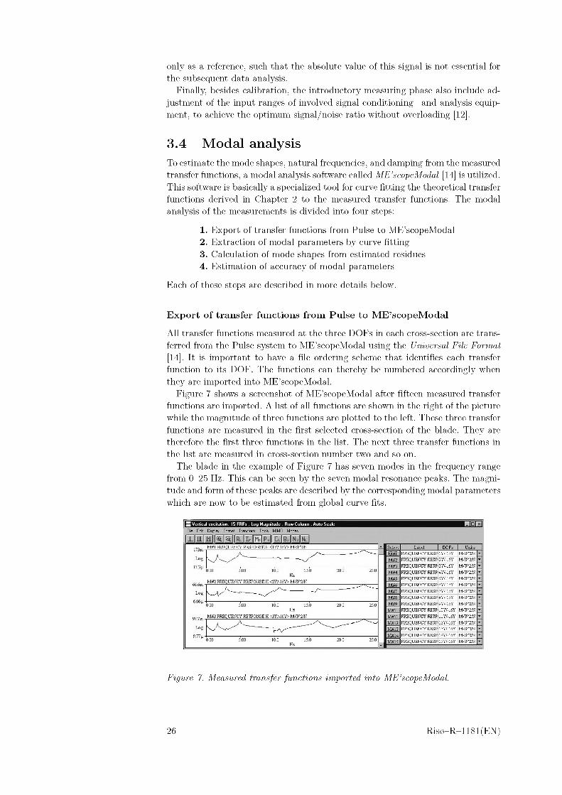
3.4 Modal analysisTo estimate the mode shapes, natural frequencies, and damping from the measured transfer functions, a modal analysis software called ME’scopeModal [14] is utilized. This software is basically a specialized tool for curve fitting the theoretical transfer functions derived in Chapter 2 to the measured transfer functions. The modal analysis of the measurements is divided into four steps:

1. Export of transfer functions from Pulse to ME’scopeModal2. Extraction of modal parameters by curve fitting3. Calculation of mode shapes from estimated residues4. Estimation of accuracy of modal parameters

Each of these steps are described in more details below.

Export of transfer functions from Pulse to ME’scopeModal

All transfer functions measured at the three DOFs in each cross-section are trans­ferred from the Pulse system to ME’scopeModal using the Universal File Format [14]. It is important to have a file ordering scheme that identifies each transfer function to its DOF. The functions can thereby be numbered accordingly when they are imported into ME’scopeModal.

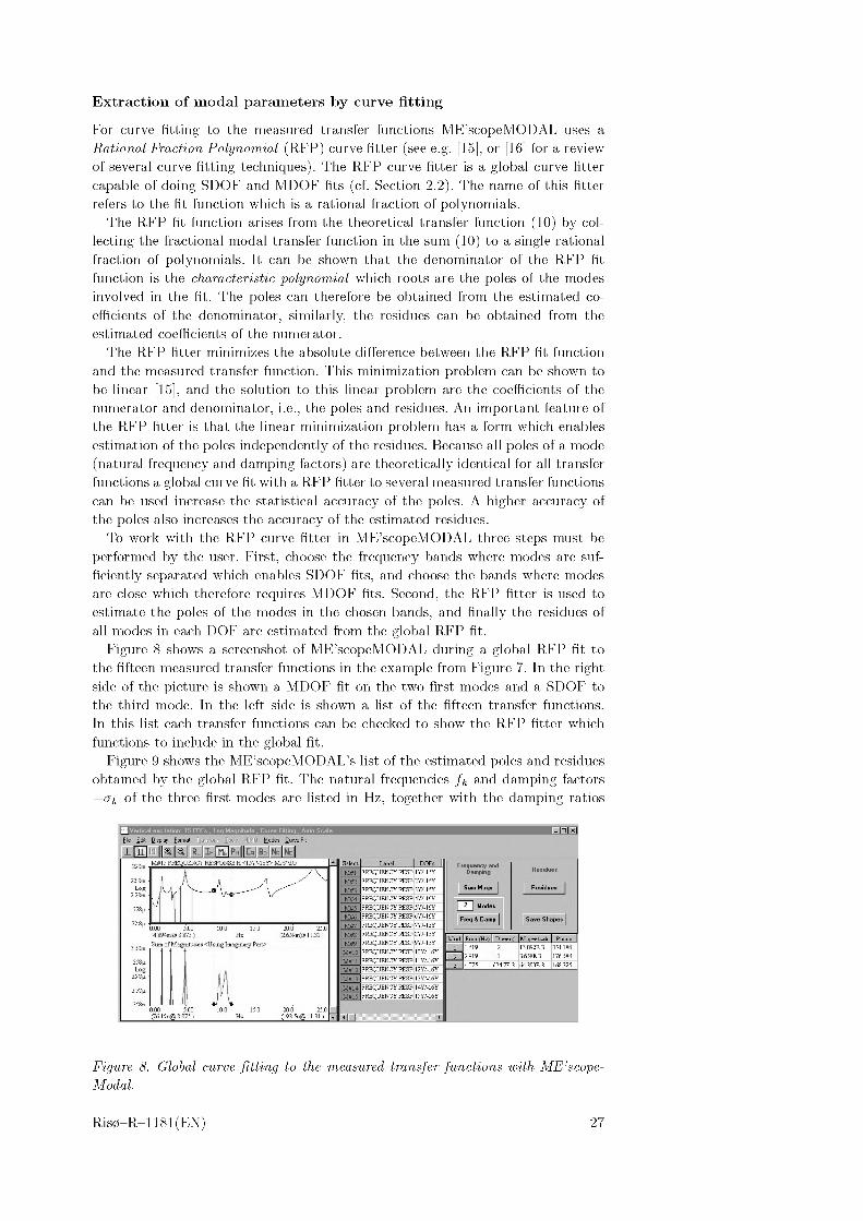
Figure 7 shows a screenshot of ME’scopeModal after fifteen measured transfer functions are imported. A list of all functions are shown in the right of the picture while the magnitude of three functions are plotted to the left. These three transfer functions are measured in the first selected cross-section of the blade. They are therefore the first three functions in the list. The next three transfer functions in the list are measured in cross-section number two and so on.

The blade in the example of Figure 7 has seven modes in the frequency range from 0-25 Hz. This can be seen by the seven modal resonance peaks. The magni­tude and form of these peaks are described by the corresponding modal parameters which are now to be estimated from global curve fits.

Figure 7. Measured transfer functions imported into ME’scopeModal.

26 Ris0-R-1181(EN)

Extraction of modal parameters by curve fitting

For curve fitting to the measured transfer functions ME’scopeMODAL uses a Rational Fraction Polynomial (RFP) curve fitter (see e.g. [15], or [16] for a review of several curve fitting techniques). The RFP curve fitter is a global curve fitter capable of doing SDOF and MDOF fits (cf. Section 2.2). The name of this fitter refers to the fit function which is a rational fraction of polynomials.

The RFP fit function arises from the theoretical transfer function (10) by col­lecting the fractional modal transfer function in the sum (10) to a single rational fraction of polynomials. It can be shown that the denominator of the RFP fit function is the characteristic polynomial which roots are the poles of the modes involved in the fit. The poles can therefore be obtained from the estimated co­efficients of the denominator, similarly, the residues can be obtained from the estimated coefficients of the numerator.

The RFP fitter minimizes the absolute difference between the RFP fit function and the measured transfer function. This minimization problem can be shown to be linear [15], and the solution to this linear problem are the coefficients of the numerator and denominator, i.e., the poles and residues. An important feature of the RFP fitter is that the linear minimization problem has a form which enables estimation of the poles independently of the residues. Because all poles of a mode (natural frequency and damping factors) are theoretically identical for all transfer functions a global curve fit with a RFP fitter to several measured transfer functions can be used increase the statistical accuracy of the poles. A higher accuracy of the poles also increases the accuracy of the estimated residues.

To work with the RFP curve fitter in ME’scopeMODAL three steps must be performed by the user. First, choose the frequency bands where modes are suf­ficiently separated which enables SDOF fits, and choose the bands where modes are close which therefore requires MDOF fits. Second, the RFP fitter is used to estimate the poles of the modes in the chosen bands, and finally the residues of all modes in each DOF are estimated from the global RFP fit.

Figure 8 shows a screenshot of ME’scopeMODAL during a global RFP fit to the fifteen measured transfer functions in the example from Figure 7. In the right side of the picture is shown a MDOF fit on the two first modes and a SDOF to the third mode. In the left side is shown a list of the fifteen transfer functions. In this list each transfer functions can be checked to show the RFP fitter which functions to include in the global fit.

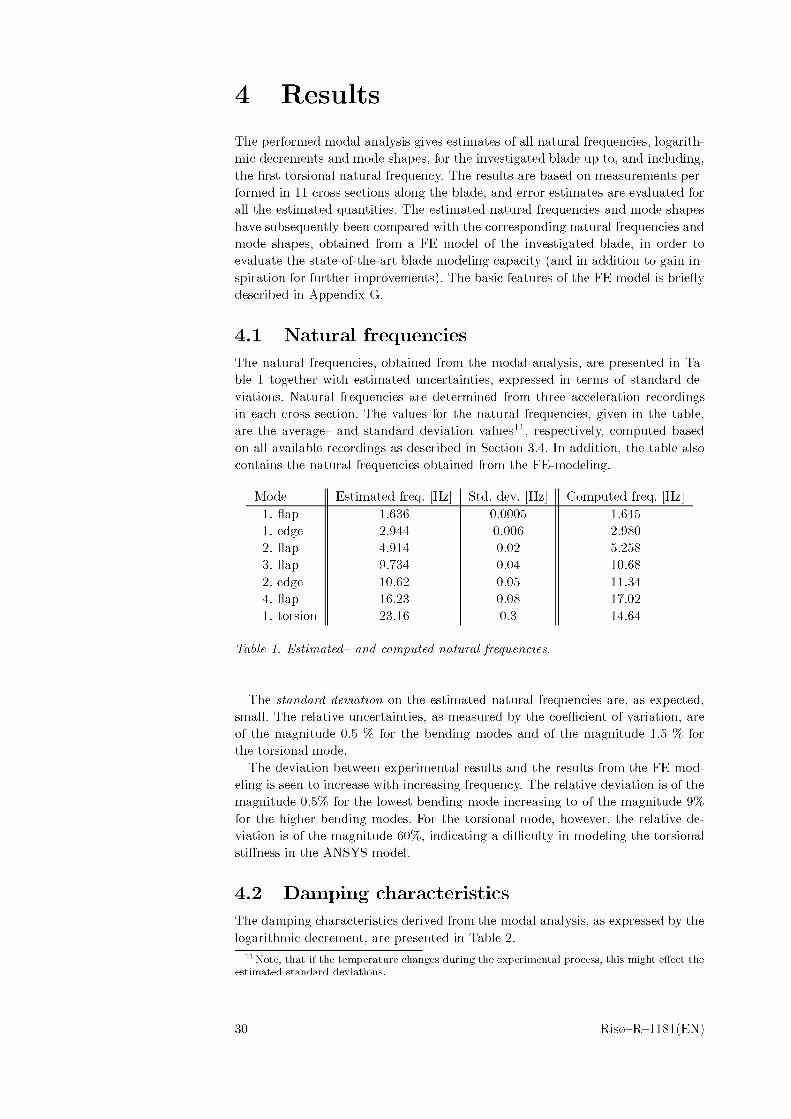
Figure 9 shows the ME’scopeMODAL’s list of the estimated poles and residues obtained by the global RFP fit. The natural frequencies fk and damping factors —ak of the three first modes are listed in Hz, together with the damping ratios

Figure 8. Global curve fitting to the measured transfer functions with. ME’scope- Modal.

Ris0-R-1181(EN) 27

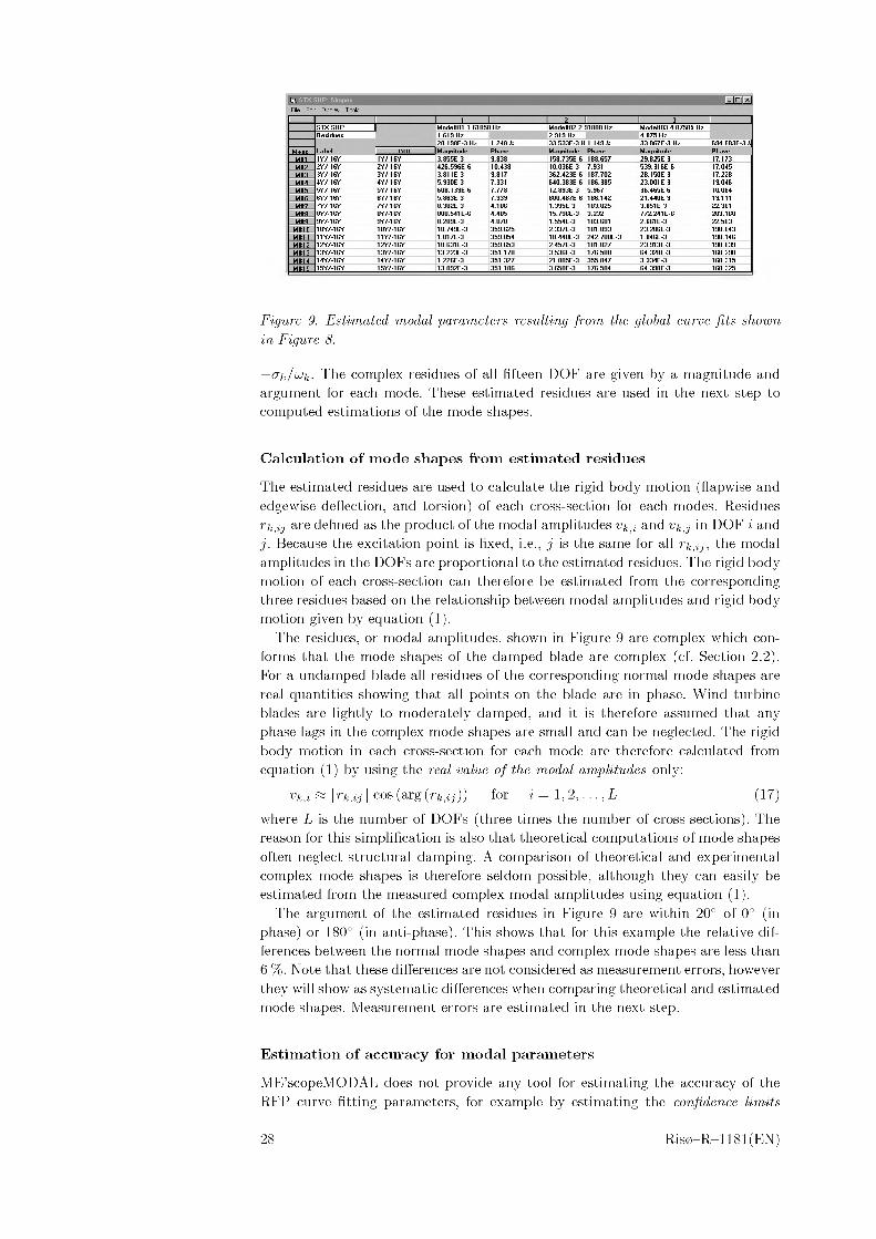
Figure 9. Estimated modal parameters resulting from the global curve fits shown in Figure 8.

-ak/ivk. The complex residues of all fifteen DOF are given by a magnitude and argument for each mode. These estimated residues are used in the next step to computed estimations of the mode shapes.

Calculation of mode shapes from estimated residues

The estimated residues are used to calculate the rigid body motion (ftapwise and edgewise deflection, and torsion) of each cross-section for each modes. Residues rkgj are defined as the product of the modal amplitudes vkg and vkj in DOF i and j. Because the excitation point is fixed, i.e., j is the same for all -rfc/y, the modal amplitudes in the DOFs are proportional to the estimated residues. The rigid body motion of each cross-section can therefore be estimated from the corresponding three residues based on the relationship between modal amplitudes and rigid body motion given by equation (1).

The residues, or modal amplitudes, shown in Figure 9 are complex which con­forms that the mode shapes of the damped blade are complex (cf. Section 2.2). For a undamped blade all residues of the corresponding normal mode shapes are real quantities showing that all points on the blade are in phase. Wind turbine blades are lightly to moderately damped, and it is therefore assumed that any phase lags in the complex mode shapes are small and can be neglected. The rigid body motion in each cross-section for each mode are therefore calculated from equation (1) by using the real value of the modal amplitudes only:

for i = l,2,...,T (17)where L is the number of DOFs (three times the number of cross-sections). The reason for this simplification is also that theoretical computations of mode shapes often neglect structural damping. A comparison of theoretical and experimental complex mode shapes is therefore seldom possible, although they can easily be estimated from the measured complex modal amplitudes using equation (1).

The argument of the estimated residues in Figure 9 are within 20° of 0° (in phase) or 180° (in anti-phase). This shows that for this example the relative dif­ferences between the normal mode shapes and complex mode shapes are less than 6 %. Note that these differences are not considered as measurement errors, however they will show as systematic differences when comparing theoretical and estimated mode shapes. Measurement errors are estimated in the next step.

Estimation of accuracy for modal parameters

ME’scopeMODAL does not provide any tool for estimating the accuracy of the RFP curve fitting parameters, for example by estimating the confidence limits

28 Ris0-R-1181(EN)

of the frequencies, damping factors, and residues. Thus other more approximate procedures for estimating the accuracy of the modal parameters have been chosen.

Standard deviations of the estimated natural frequencies and damping factors are calculated from L individual estimates. These estimates are obtained by using ME’scopeMODAL to perform L local curve fits to each measured transfer func­tions. The standard deviations based on this procedure are conservative estimates of the accuracy of the natural frequencies and damping factors obtained from the global RFP curve fits because local curve fits are less accurate than global fits.

To estimate the accuracy of the mode shapes it is necessary to estimate the error on the modal amplitudes (residues) and on the DOF geometry (positions and directions of the three DOFs) as it is described in Appendix B. The accuracy of the modal amplitudes cannot be estimated by calculating standard deviations based on multiple local curve fits because each transfer function only describe one residue for each mode. Instead it is assumed that the relative error of each residue rk,ij can be approximated by the relative standard deviation of the measured transfer function Hj in the vicinity of the corresponding modal peak k. The relative standard deviation of the points in a transfer function is estimated from the corresponding coherence functions Yj using relation (16). Thus, by taking an average of the coherence function in a frequency range enclosing each modal peak of each transfer function, local estimates of the error on the modal amplitudes can be obtained. The errors on the positions and directions of the DOFs on the blade must be estimated by considering the accuracy of the setup and measurement of the geometry (Section 3.3). After the errors on the modal amplitudes and DOF geometry are estimated, the variance (squared standard deviation) of the mode shape can be calculated from expression (B.4) in Appendix B.

Ris0-R-1181(EN) 29

4 Results

The performed modal analysis gives estimates of all natural frequencies, logarith­mic decrements and mode shapes, for the investigated blade up to, and including, the first torsional natural frequency. The results are based on measurements per­formed in 11 cross sections along the blade, and error estimates are evaluated for all the estimated quantities. The estimated natural frequencies and mode shapes have subsequently been compared with the corresponding natural frequencies and mode shapes, obtained from a FE model of the investigated blade, in order to evaluate the state-of-the-art blade modeling capacity (and in addition to gain in­spiration for further improvements). The basic features of the FE model is briefly described in Appendix G.

4.1 Natural frequenciesThe natural frequencies, obtained from the modal analysis, are presented in Ta­ble 1 together with estimated uncertainties, expressed in terms of standard de­viations. Natural frequencies are determined from three acceleration recordingsin each cross section. The values for the natural frequencies, given in the table, are the average- and standard deviation values11, respectively, computed based on all available recordings as described in Section 3.4. In addition, the table alsocontains the natural frequencies obtained from the FE-modeling.

Mode Estimated freq. [Hz] Std. dev. [Hz] Computed freq. [Hz]1. flap 1.636 0.0005 1.6451. edge 2.944 0.006 2.9802. flap 4.914 0.02 5.2583. flap 9.734 0.04 10.682. edge 10.62 0.05 11.344. flap 16.23 0.08 17.021. torsion 23.16 0.3 14.64

TbWe 1. Estimated- and competed natwa//regwencies.

The standard deviation on the estimated natural frequencies are, as expected, small. The relative uncertainties, as measured by the coefficient of variation, are of the magnitude 0.5 % for the bending modes and of the magnitude 1.5 % forthe torsional mode.

The deviation between experimental results and the results from the FE mod­eling is seen to increase with increasing frequency. The relative deviation is of the magnitude 0.5% for the lowest bending mode increasing to of the magnitude 9% for the higher bending modes. For the torsional mode, however, the relative de­viation is of the magnitude 60%, indicating a difficulty in modeling the torsional stiffness in the ANSYS model.

4.2 Damping characteristicsThe damping characteristics derived from the modal analysis, as expressed by the logarithmic decrement, are presented in Table 2.

11 Note, that if the temperature changes during the experimental process, this might effect the estimated standard deviations.

30 Ris0-R-1181(EN)

Mode Estimated log. decrement [%] Std. dev. [%]1. flap 1.78 0.081. edge 3.60 0.012. flap 2.02 0.013. flap 2.47 0.032. edge 5.57 0.044. flap 3.23 0.031. torsion 5.81 0.06

Tdh/e Estimated damping characteristics eapressed as /ogarithmic decrement.

The damping is as expected, for a given type of mode (flap dominated, edge dominated or torsion dominated), increasing with increasing natural frequency. As previously mentioned, the investigated blade has been designed with an es­pecially high edgewise damping, which is also reflected in the measured damping characteristics.

Determination of the damping properties is usually considered to be somewhat uncertain, which relates to the fact that the damping characteristics are small quantities. For the present results, however, the relative uncertainty (measured in terms of the coefficient of variation) is only of the magnitude 1%, except for the first flapwise mode, where the estimated coefficient of variation turned out to be of the magnitude 5%. The damping depends on temperature, and therefore the apparent uncertainty will increase if the temperature is changing during the measuring campaign.

4.3 Mode shapesThe mode shape results, associated with the lowest 7 blade natural frequencies, are illustrated in Figure 10 - 16. For each particular mode, the modal deflectionhas been resolved in a flapwise, an edgewise and a torsional deflection, according to the definitions given in Chapter 2. For each deflection component, the discrete results obtained from the modal analysis have been compared to the eigenforms obtained from the FE-modeling. In order to facilitate the comparison, the cross section rotation, associated with the FE-modeling, is defined as the rotation of a line connecting the leading edge with the tailing edge for a given cross section. In analogy, the bending deflection is defined as the deflection of a radial spline, along which the longitudinal web is attached to the blade surface. Note, that this definition is not necessary kinematic consistent and analog to the definition presented in Appendix A for the modal analysis.

A mode shape is uniquely determined apart from an amplitude. For the present illustration it was, arbitrary, chosen to normalize the dominating tip deflection component in each mode to 1 m in case of a displacement and to 10 deg in case of a torsion. The torsion, however, is not well determined in the tip section. Due to the very short cord length associated with this particular cross section, it was necessary to apply a different support structure here compared to the other cross sections. Caused partly by smaller dimensions of this more primitive measuring bridge, partly by difficulties with fixing even this measuring bridge to the tip cross section, the torsion resolution in the tip turned out to be unsatisfactory. Consequently, for the normalization, the tip torsion has been evaluated by extrapolation of the nearby cross-section torsional values.

Ris0-R-1181(EN) 31

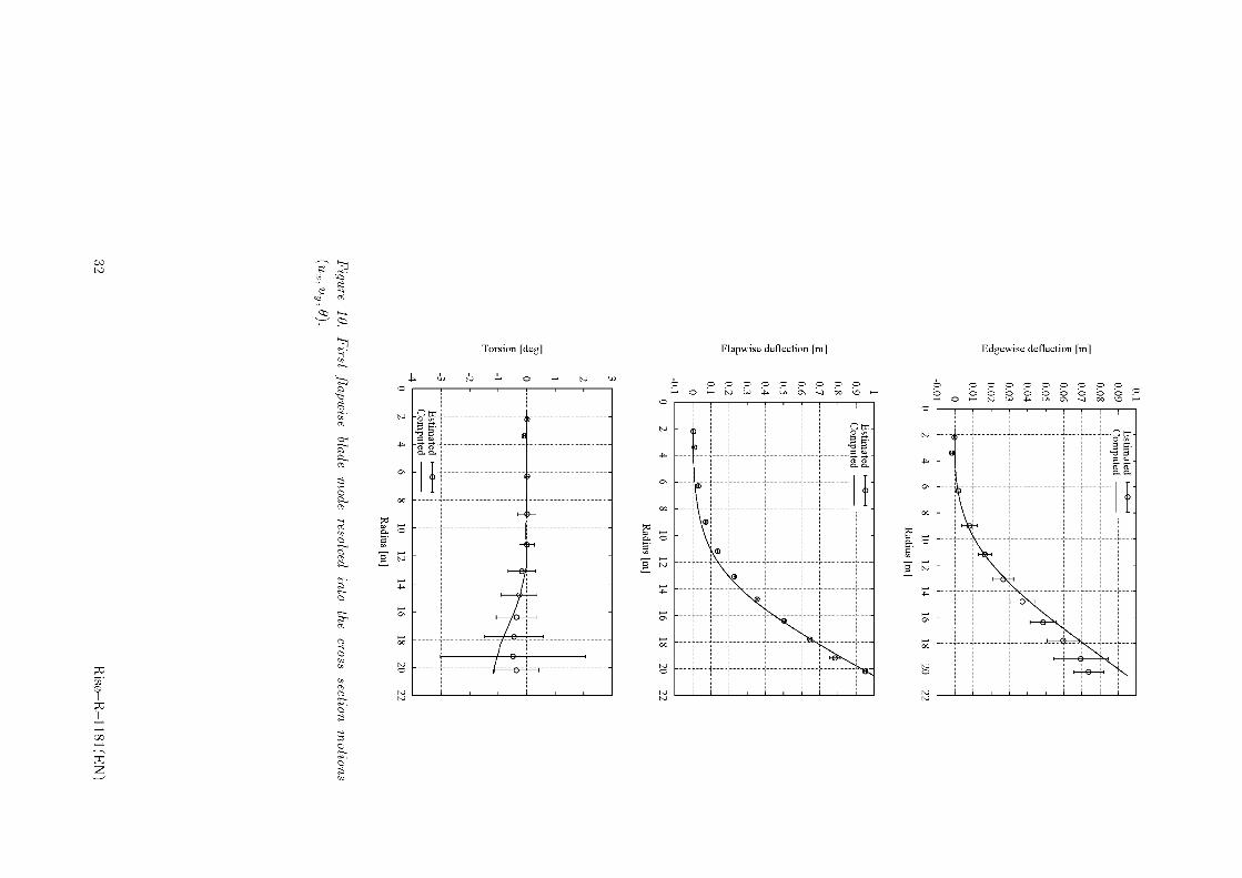
Ris0-R

-1181 (EN)

COto

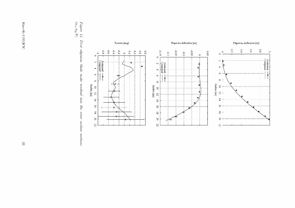
&l

g

COCO

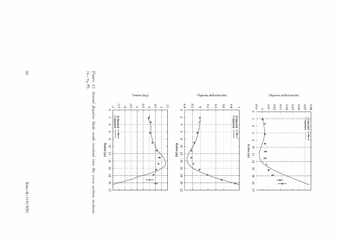
Ris0-R

-1181 (EN)

CO

e-i

81

I

©Aw

A-

01|©

Sr

Torsion [deg] Flapwise deflection [m] Edgewise deflection [m]

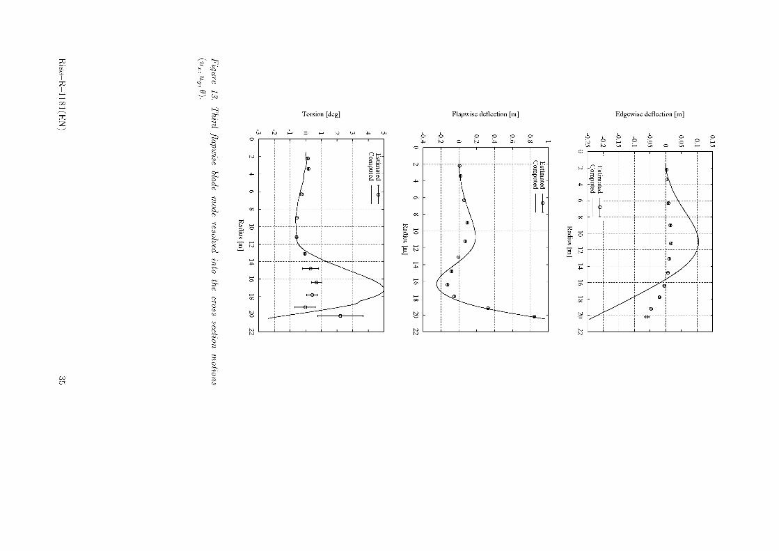
&l

g

COCn

<1£

Co

9

I

©Aw

5-

Torsion [deg] Flapwise deflection [m] Edgewise deflection [m]

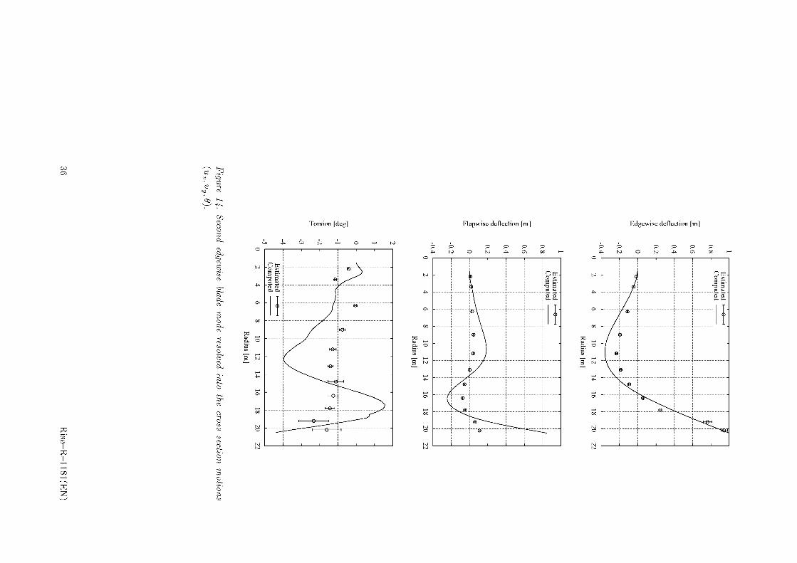
Ris0-R

-1181 (EN)

COa

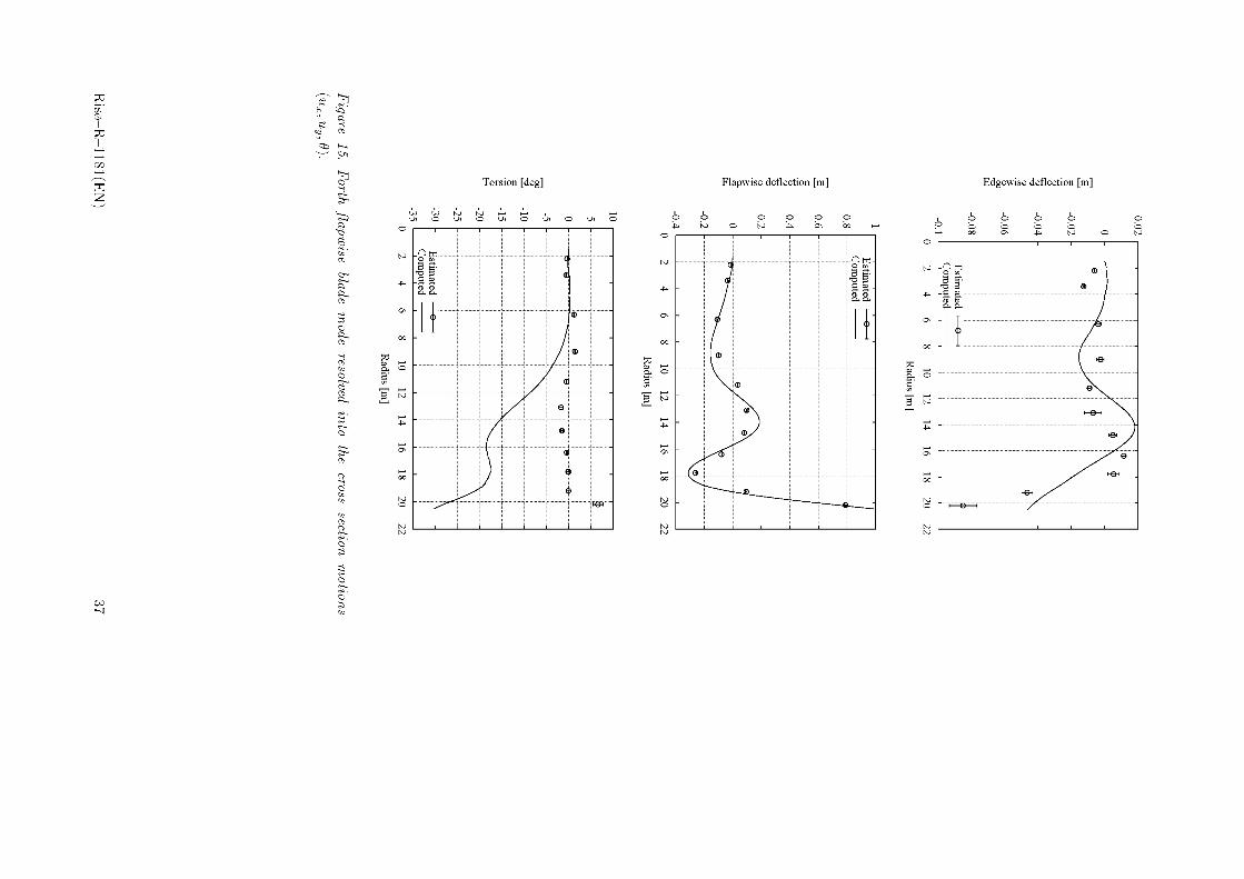
&l

g

CO-I

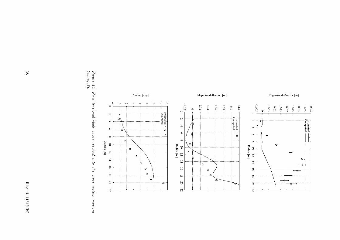
Ris0-R

-1181 (EN)

CO00

In general, the mode shapes extracted from the modal analysis display the ex­pected smooth behaviour without notable scatter except for the torsion of the tip cross section. The reason for the unsatisfactory representation at the tip is com­mented on above. For all the investigated mode shapes, the dominating deflection component resembles the same general features, comparing the results from the modal analysis with the corresponding results from the FEM analysis. However, the agreement is better for the deflection components associated with low nat­ural frequencies than for deflection components associated with higher natural frequencies. The same tendency was also observed in the estimation of natural frequencies.

Discussion

The test stand has a certain (small) flexibility. This flexibility is neglected in the FE modeling of the LM 19 m blade as described in Appendix G. The effect from this deviation in the boundary conditions at the blade root between experiment and FE-model, respectively, can be identified from the present results. The mode shape gradient in the root part tend to be larger for the experimental results than for the FEM results. The neglection of the elasticity of the tip brake mech­anism in the FE modeling, however, does not seem to cause differencies between experimental- and FEM results - hence it follows that this flexibility does not affect the mode shapes.

The structural coupling, between the dominating deflection and the two re­maining (secondary) deflection components, is identified for all the analysed mode shapes both experimentally and numerically. The coupling between bending de­flection and torsion requires special attention due to the direct implications for the aerodynamic loading. This coupling is of course especially important for the mode shapes associated with the lower and most important natural frequencies. For these modes, a tip deflection of 1 m corresponds to a torsion of the magnitude 0.5 deg due to the structural coupling.

Aeroelastic calculations are traditionally based on a Timoshenko beam model­ing of the wind turbine blade. Although the bending torsion couplings usually are included in the beam representation, the correct specification of these structural couplings is a delicate matter. The magnitude of the observed bending/torsion coupling effects suggests, that these may significantly affect the aerodynamic load characteristics of a wind turbine blade. This emphasizes the need for careful spec­ification of such coupling effects in aeroelastic computations. Also the structural coupling between the two bending components is essential for correct modeling of aerodynamic damping [13]. This coupling is often included in the aeroelastic model by introducing a structural pitch. The relevant structural pitch for the LM 19 m blade can easily be derived from the present results.

In general, the deviation between experimental and modeled secondary deflec­tion components is larger than the difference between the corresponding primary deflection components, reflecting that these deflections are difficult to resolve ex­perimentally (small signal levels) as well as numerically (lack of sufficiently detailed information on the material properties). As with the primary deflections, there is a tendency towards increasing deviation between experiment and numerical results with increasing frequency. Except for the two modes associated with the highest natural frequencies, the numerical model is seen to over estimate the structural couplings.

Ris0-R-1181(EN) 39

5 Conclusion

The present investigation has demonstrated that essential dynamic properties of wind turbine blades, like natural frequencies, damping characteristics and mode shapes, can be experimentally determined by use of the modal analysis technique. Different experimental procedures have been considered and the most appropriate of these has been selected. Although the comparison is based only on measure­ments on a LM 19 m blade, the recommendations given are believed to be valid for other types (sizes, designs, ...) of wind turbine blades as well.

The reliability of the selected experimental analysis has been investigated by estimating the unsystematic variations in the experimental findings. The unsys­tematic deviations have been quantified in terms of standard deviations and co­efficients of variations. In general, the estimated standard deviations on natural frequencies and damping characteristics indicate a high degree of reliability. For the modal shapes, however, the accuracy vary with the mode number. For the dominating deflection direction, associated with a particular natural frequency, the uncertainty is very modest. For the two ’’secondary” deflection directions the standard deviations on the cross sectional deflections are somewhat larger - espe­cially for the torsional deflection.

In addition to the unsystematic variations, systematic errors caused by theexperimental technique (e.g. elasticity of the blade support, heavy sensor setup mounted on the blade, or errors in the measurement of the applied reference axis) as well as the signal processing (windowing etc.) may occur. No attempt has been made to quantify such errors.

The detailed analysis of the LM 19 m blade has been compared with results from a FE-model of the same blade. For some of the higher modes substantial discrepancies between the natural frequencies originating from the FE-modeling and the modal analysis, respectively, are observed. This is especially pronounced for the torsion mode indicating a defective modeling of the torsional stiffness. Turning to the modal shapes, the agreement between experimental results and the present FE-model is generally good concerning the dominating deflection, indicating that the relative stiffness distributions applied in the FE-model are satisfactory. However, large discrepancies are seen in the ” secondary” deflection directions which may be due to both the relative high experimental uncertainty in the determination of those, and to an insufficient representation of structural couplings in the FE-model.

The performed comparison between experimental- and FEM results emphasizes the need for this kind of experimental results to refine the modeling technique. Also the observed uncertainty in some of the experimental results calls for im­provements of the experimental technique.

The main disadvantage of the proposed impact test is that the force excitation level is not invariant from one test to another. As a consequence the global response of the global structure, including linear as well as non-linear components, change in an unpredictable manner. Non-linear components of the structural response might be important and can potentially create errors which are difficult to quantify. The last disadvantage is the possible variation of the force direction from one test to another (which, however, is reduced using the guided hammer) introducing errors in the evaluation of the structure egenvectors.

In order to overcome the above mentioned problems with manually operated im- pactors, electromechanical slave hammers can be used [2]. The hammer works with the principle of an electromagnet, where two coils are independently pushing and pulling a piston. The coils are connected to power circuits that produce rectangu­lar signal of current, with predefined levels, duration, and time delay. This means

40 Ris0-R-1181(EN)

desirable possibilities to control velocity and retardation just before the impact, in order to avoid multiple rebounds. A ”cleaner” impact together with the ability of producing replicated impacts with repetitive characteristics, can here significantly improve the force/response correlation compared to the manually operated ham­mer, especially in the lower frequency range. An additional feature, that comes with the control, is the possibility to simultaneously operate several impactors, resulting in multipoint excitation (polyreference method). The idea of a repetitive slave hammer can also be realized using pneumatic, or hydraulic actuators (see for example [10]).

In addition to potential future modifications of the exciter system, larger wind turbine blades, with their very low natural frequencies, may require use of DC- accelerometers (or other types of low frequency sensitive accelerometers) insteadof the piezoelectric accelerometers used in the present investigation, in order to improve the quality of the estimated transfer functions and thus the quality of the modal analysis.

Ris0-R-1181(EN) 41

Acknowledgements

The work, presented in this report, has been funded by the Danish Ministry of Energy in the contract ENS 1363/98-0010. S0ren M. Pedersen, Ris0, is grate­fully acknowledged for assisting in performing the last part of the experimental campaign. J0rgen T. Petersen and Morten Th0gersen, Ris0, are acknowledged for making the results from their FE modeling of the LM 19 m blade available for the comparative analysis presented in the report.

42 Ris0-R-1181(EN)

References

[1] Halvorsen, W.G. and Brown, D.L. (1977). Impulse Technique for Structural Frequency Response Testing. Sound and Vibration, Vol. 11, No. 11, 8-21.

[2] Tawfiq, T.V. and Vinh, T. (1997). A new Approach to Impact Testing In­strumentation using an Electronic Slave Hammer. Mechanical Systems andSignal Processing, 11(2), 269-285.

[3] Bruel & Kj$r (1998). Getting Started - An Introduction to PULSE Software. Bruel & Kj$r, Denmark.

[4] Randall, B. (1987). Frequency Analysis. Bruel & Kj$r, Denmark.

[5] Edwins, D.J. (1986). Modal Testing: Theory and Practice. Research Studies Press Ltd. and. Bruel & Kj$r.

[6] Madsen, H.AA. (ed.) (1999). Forskning i Aeroelasticitet - EFP-98. Ris0-R- 1129 (in Danish).

[7] Experimental modal analysis for WTS-3 wind turbine (1981). Report HSER8205, Hamilton standard division of United Technologies Corporation (re­stricted).

[8] Larsen, G.C. and Kretz, A. (1995). Experimental Determination of Stiffness Distributions and Mode Shapes of Wind Turbine Blades. Ris0-R-773(EN).

[9] Bendat, J.S. and Piersol, A.G. (1995). Random Data - Analysis and Mea­surement Procedures. John Wiley & Sons, Inc..

[10] Philippidis, T.P., Vionis, P.S., Lekou, D.J. and Fragoulis, A.N. (1997) Rotor Blade Design Verification by means of Full Scale Testing. Proceedings of EWEC97, Dublin, Ireland.

[11] Newland, D.E. (1984). Random Vibration and Spectral Analysis. Longman Scientific & Technical.

[12] B&K PULSE system. On-line Manual.

[13] Petersen, J.T., Madsen, H.Aa., Bjork, A., Enevoldsen, P., 0ye, S., Ganan- der, H. and Winkelaar, D. (1998). Prediction of Dynamic Loads and InducesVibrations in Stall. Ris0-R-1045(EN).

[14] ME’scope™ Operating Manual (1997). Version 4.0. Vibrant Technology, Inc..

[15] Richardson, M.H. (1986). Global Frequancy and Damping Estimates from Frequency Response Measurements. Proceedings of 4RD IMAC Conference, Los Angeles, CA, USA.

[16] Allemang, R.J. and Brown, D.L. (1998). A Unified Matrix Polynomial Ap­proach to Modal Identification. Journal of Sound and Vibration, Vol. 211, No. 3, 301-322.

Ris0-R-1181(EN) 43

44 Ris0-R-1181(EN)

A Discrete blade motion

In this appendix it is shown how to calculate the rigid body translation and rotation of a cross-section based on three amplitudes of vibration measured in three degrees of freedom (DOFs). The configuration of DOFs influences the accuracy of the mode shape estimations. This influence is discussed based on a sensitivity analysis of the derived expressions.

Figure 17 shows a cross-section with three “transducers” measuring the trans­lation in three DOFs given by their directions (a*, ai+1, ai+2) and positions (ri; ri+i, ri+2) with respect to the pitch-axis (cf. Figure 1). When the cross-section is undergoing a rigid body motion given by translations ux and uy, and a rotation 6 about the pitch-axis, the displacement vector w* for measurement point i is:

Wi uxuy

+ (T - I) r*, (A.1)

where I is a two by two identity matrix, and T is a transformation matrix:cos 6 - sin 6sin 6 cos 6 (A.2)

The measured amplitude in DOF number i is x*, which can also be considered as the projection of vector w* onto the direction of the DOF a*. Assuming that the rotation of the cross-section due to torsion is small (6 < 1), a linear relationshipbetween the rigid body motion and the amplitude x* is obtained

x* = Ux cos a* +uy sin a* + (r? sin a* — ry cos a*) 6. (A.3)Similarly, the measured amplitudes in all three DOFs yields a set of three equations which by inverting can be written as

uxuy A < x*+i

[ X*+2

x

6(A.4)

where the matrix A is given by

Asin a*

sin a*+ir*x sin a* — r*y cos a*

rX+i sin Oj+i — r|+i cos a*+icos a*

cos a*+icos a*+2 sin a*+2 rx+2 sin a*+2 — r*+2 cos a*+2

Note, that the rigid body motion of the cross-section is not tion (A.4) for all configurations of DOFs because the matrix Other percussions must also be considered (cf. Appendix B).

-i

. (A.5)

described by rela- A may not exist.

Tr

w,

r

F^gwre 47. R«g»d 6odg motion (Ux, uy, 6j o/a cross-sec^oM g^^em 6g tAree degrees o//reedom (x*, x*+i, x*+2j.

Ris0-R-1181(EN) 45

46 Ris0-R-1181(EN)

B Errors on mode shapes

In this appendix it is shown how to derive the standard deviations on mode shapesdue to error on estimated modal amplitudes and on the configuration of DOFs. From this derivation it is then shown how to optimize the configuration of DOFs for minimum error.

B.1 Expression for the error on mode shapesTo derive an expression of the error on a mode shape vector u = {ux, uy, 0}T of each cross-section, it is assumed that the error on the estimated modal ampli­tudes and geometry of the DOF configuration are small. Defining a book-keeping parameter for small quantities as e < 1 this assumption can be written as

x = x+eAx , r = ri+eAr , and a = a +eAa , (B.1)

where the bar denotes estimated quantities, and vector x = {xi,xi+1 ,xi+2}Tcontains the modal amplitudes of the particular cross-section which errors are given by Ax. The error on the position and direction of the three DOFs is given by Ari+k and Aai+k with k = 0,1,2.

The modal amplitudes and DOF geometry (B.1) are used to estimate a mode shape vector which will be subject to error described as U + eAu. To derive an expression for Au the equation (B.1) is inserted into equation (1) which, after Taylor expansion of transformation matrix A (A.5), yields

u+ eAu = A + eyr 9A

k=0 ^+kArX+k + e

^ 9A 2-v arv k=0 i+k

Arf+k

+e2 - 9A

k=0 i+kAai+k + O(e2 ) I (x + eAx), (B.2)

where O(e2) denotes higher order terms, and bar over matrices show that they are evaluated at the estimated DOF geometry ri+k and ai+k with k = 0,1,2. Collect­ing terms of order e0 shows that u = Ax which corresponds to equation (1) used for calculating the estimate of the mode shapes in each cross-section. Collecting terms of order e1 yields

Au A AX + J2 dA0^

Arx+k+yi dA

oAry+k +

2 - 9A Aaik=0 i+k

i+k2

x ,

(B.3)

where matrix AX = diag{Axi/xi, Axi+1/xi+1, Axi+2/xi+2} contains the relative errors on the modal amplitudes. The sum of matrices in the brackets of (B.3) is subsequently denoted AA.

Because the sign of the errors on modal amplitudes and DOF geometry is un­known we use equation (B.3) to derive the variance matrix of the errors on the mode shapes as function of the relative variance on the modal amplitudes and the absolute variance on the position and direction of the DOFs. Using that x = A-1u the variance matrix of the errors on the mode shapes becomes

AuAuT = AAA-1uuT (AAA_1)T . (B.4)

The standard deviations on the mode shapes can now be calculated as the squareroot of the diagonal elements of this variance matrix AuAuT.

Ris0-R-1181(EN) 47

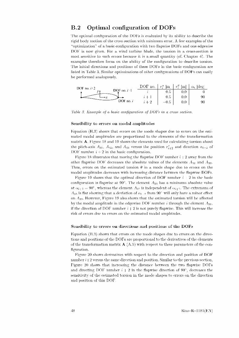
B.2 Optimal configuration of DOFsThe optimal configuration of the DOFs is evaluated by its ability to describe the rigid body motion of the cross-section with minimum error. A few examples of the “optimization” of a basic configuration with two flapwise DOFs and one edgewise DOF is now given. For a wind turbine blade, the torsion in a cross-section is most sensitive to such errors because it is a small quantity (cf. Chapter 4). The examples therefore focus on the ability of the configuration to describe torsion. The initial directions and positions of these DOFs in the basic configuration are listed in Table 3. Similar optimizations of other configurations of DOFs can easily be performed analogously.

DOF no. i+2 DOF no. i+1DOF no. rf [m] rf [m] [deg]

t y\ % 0.5 0.0 0i+1 0.5 0.0 90

DOF no. i i + 2 -0.5 0.0 90

TbWe Fzarnp/e o/ a o/ DOFs rn a cross-sectwM.

Sensibility to errors on modal amplitudes

Equation (B.3) shows that errors on the mode shapes due to errors on the esti­mated modal amplitudes are proportional to the elements of the transformation matrix A. Figure 18 and 19 shows the elements used for calculating torsion about the pitch-axis A31, A32, and A33 versus the position rf+2 and direction ai+2 of DOF number i + 2 in the basic configuration.

Figure 18 illustrates that moving the flapwise DOF number i + 2 away from the other flapwise DOF decreases the absolute values of the elements A32 and A33. Thus, errors on the estimated torsion 0 in a mode shape due to errors on the modal amplitudes decreases with increasing distance between the flapwise DOFs.

Figure 19 shows that the optimal direction of DOF number i + 2 in the basic configuration is flapwise at 90°. The element A33 has a minimum absolute value at ai+2 = 90°, whereas the element A32 is independent of ai+2. The extremum of A33 is flat showing that a deviation of ai+2 from 90° will only have a minor effect on A33. However, Figure 19 also shows that the estimated torsion will be affected by the modal amplitude in the edgewise DOF number i through the element A31, if the direction of DOF number i + 2 is not purely flapwise. This will increase the risk of errors due to errors on the estimated modal amplitudes.

Sensibility to errors on directions and positions of the DOFs

Equation (B.3) shows that errors on the mode shapes due to errors on the direc­tions and positions of the DOFs are proportional to the derivatives of the elements of the transformation matrix A (A.5) with respect to these parameters of the con­figuration.

Figure 20 shows derivatives with respect to the direction and position of DOF number i+2 versus the same direction and position. Similar to the previous section, Figure 20 shows that increasing the distance between the two flapwise DOFs and directing DOF number i + 2 in the flapwise direction of 90°, decreases the sensitivity of the estimated torsion in the mode shapes to errors on the direction and position of this DOF.

48 Ris0-R-1181(EN)

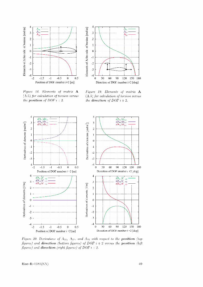
Position of DOF number i+2 [m]

Figure 18. Elements of matrix A (A.5) /or m/cwWioM o/ for+on, oersws the position of DOF i + 2.

90 120 150 180Direction of DOF number i+2 [deg]

Figure 19. Elements of matrix A (A.5) /or m/cwWioM o/ for+on, oersws the direction of DOF i + 2.

(/Av/(Zt,

0 30 60 90 120 150 180Direction of DOF number i +2 [deg]

0 30 60 90 120 150 180Position of DOF number i +2 [m] Direction of DOF number i +2 [deg]

Figure 20. Derivatives of A-n, A32, and A33 with. respect to the position (top figures) and direction (bottom figures) of DOF i + 2 versus the position (left figures) and direction (right, figures) of DOF i + 2.

Ris0-R-1181(EN) 49

50 Ris0-R-1181(EN)

C Optimum transfer function

In the absence of noise, the response of an ideal linear constant parameter physical system to some input (forcing) can be expressed as a convolution of the system impulse response function and the particular input [9], Due to the convolution, this relation is conveniently expressed in the frequency domain, where the Fourier transform of the response equals the product of a transfer function and the Fourier transform of the system input (cf. equation (5)). The transfer function is simply the Fourier transform of the system impulse response function.

Deterministic single-input/single-output system

Let us consider the simple single-input/single-output system defined as the forcing (acting in DOF number j) of a wind turbine blade and the respective response of the i’th DOF. In the ideal situation, with absence of noise in input- as well as output signals, these signals are of a pure deterministic character12, and the corresponding Fourier transforms are consequently not encumbered with statistical uncertainty. The ideal transfer function, Hjj, can thus be computed directly from the definition given in equation (5), which states

= (c.i)

where Xi(uj) denotes the Fourier transform of the output signal, and Fj(uj) is the Fourier transform of the input signal, respectively.

Single-input/single-output system with extraneous noise

Unfortunately, the system described above is a theoretical abstraction. For the real physical wind turbine blade system, the recorded forcing, as well as the recorded response, will consist of the ideal signal superimposed by an extraneous noise contribution caused by the recording system. Considering the forcing acting in DOF number j and the response measured in DOF number i, the situation is illustrated in Figure 21.

(+}*------FA<°)

F,'(w)

> H0(a>) A", (a) »A",'(w)

Figure 21. Single-input/single-output system, with extraneous noise.

Decomposing the observed force signal, /•(#), into an actual signal, fj{t), and a noise contribution, nf(t), we have

fj{t) = + • (C.2)12For the present investigation transient deterministic excitation has been selected; cf. Chapter

3. In case continuous excitation of random character is selected, estimation of the system transfer function can be performed using the algorithm dedicated for signals including noise components. This algorithm is addressed in the last part of this Appendix.

Ris0-R-1181(EN) 51

Analogous, decomposing the observed response signal, xj(t), into an actual sig­nal, xi(t), and a noise contribution, nf(t), we obtain

= Xi(t)+nx(t) (C.3)

The Fourier transforms of the apparent force- and response signals, respectively,are obtained directly from the equations (C.2) and (C.3) as

M=M+,j j (C.4)

X«H= %i(w)+NX(w),

where an upper index t refers to the apparent (or total) signal, Nf denotes the Fourier transform of the noise on the input signal, and Nf denotes the Fourier transform of the noise on the response signal.

We now turn to estimation of the system transfer function based on the observed signals. Different possibilities exists. A straight forward possibility is to general­ize equation (C.1) by replacing the Fourier transforms of the actual signals with the Fourier transforms of the apparent signals. The associated estimated transfer function, Hij (w), is thus expressed by

Hij (w) (C.5)

However, this estimation strategy has some serious draw backs. First of all, it is only based on one particular realization of the random noise contribution, andthus only a single (raw) estimate of the Fourier transforms of the noise contri­butions. The consequence is, that these Fourier transforms, in general, will be encumbered with significant statistical uncertainty. An acceptable estimate of the transfer function is thus only achieved, if the input noise and the response noise are (very) small relative to the input signal and the response signal, respectively. In other situations the transfer function estimate, given by equation (C.5), will not be appropriate to characterize neither the ideal system, nor the recorded sys­tem. Even though, the requested relationship, between the Fourier transforms of the observed input- and output signals, are identically satisfied by the transfer function, estimated according to equation (C.5), for this particular realization of recorded input- and output signals, the same transfer function estimate, applied to other realizations of input- and response signals, would most likely lead to significant inconsistencies.

A more appealing approach is to aim for a transfer function estimate that, in an average sense, will give the best possible (linear) characterization of therelationship between the observed input- and response signals - the optimum transfer function. This is the topic for the remaining part of this Appendix.

The optimum transfer function estimate

Let Hj (w) be any estimated (linear) transfer function connecting the system input signal with the system response signal. Due to the random noise components inherent in both the input signal and the response signal, it is not possible to define a transfer function that reflects a perfect correlation between arbitrary realizations of the input- and response signals. However, as indicated above, we can determine a transfer function that provides the best possible correlation in an average sense. For this purpose, let the observed system be described by

%f(w) Hij(w)ff(w)+Nr(w), (C.6)

52 Ris0-R-1181(EN)

where the residual noise term Ni'3(w) accounts for the lack of perfect correlation between an arbitrary forcing acting in DOF number j and the corresponding response measured in DOF number i. Note, that no assumptions has been put on this noise term. Isolating the residual noise term from equation (C.6), the followingrelation is obtained

NT(w) = X«(w) -Hij(w)fj(w). (C.7)

The residual noise term will, in general, be a complex quantity like the otherterms in equation (C.7). The size of the noise term, in an energy sense, is conse­quently obtained by multiplying Ni'3 (w) by its complex conjugate given by

(C.8)

where an ” overbar” denotes complex conjugate. The magnitude of the residualnoise component is then given by

(C.9)

Following the definition of (one-sided) spectra, as given in [9], for sample recordsof length T, the autospectrum of the residual noise noise component is expressed by

4TH lim (C.10)

where (■) denotes ensemble averaging. Introducing equation (C.9) in equation (C.10), the residual noise autospectrum is expressed in terms of the (observed) input- andresponse spectral quantities as follows

SRR(w) = X (w)-Hj(w)SF X (w)-Hij(w)SX F (w)+Hij(w)Hj(w)SF F (w),(C.11)

where the lower indices, i and j, indicate that the forcing is applied in DOFnumber j, and the respective response is observed in DOF number i. SFj F (w) denotes the apparent input autospectrum, and SX*X (w) is the apparent response autospectrum. The cross spectra between the apparent input and response signals, denoted by SF x (w) and Sx3 F (w), respectively, are defined by

S^ *F * (w)

Sj X * (w)(C.12)

From equations (C.12) the following relation between cross spectra is derived

SFX * Sij (w) s:X*F* (w) (C.13)

We now return to the expression for the residual noise autospectrum, as givenin equation (C.11), and define the optimum transfer function as the least squares estimate, Hj (w), that minimizes SRR(w) over all possible definitions of (linear) transfer function estimates.

Ris0-R-1181(EN) 53

All quantities in equation (C.11) are real valued, except the transfer functionand the cross spectra. Decomposing the complex quantities in real and imaginary parts, denoted by upper indices R and I, respectively, we obtain

Hij(w) = HR(w) - iHHR(w),

Hij (w) = HHR (w) + iHHR (w),

-,F *X _ oF*X R \ _ oF *X tI'SFX (w)= SF (w) - iSFX (w),t vt I

4 " (w) = ^ (w) = ^R ^ (w) + i^R ^ H .

Introducing equations (C.14) in equation (C.11) finally yields

(C.14)

SRR(w) = SX X(w) - 2HR(w)SRtxtR(w) - 2HR(w)SRtx tI

(jHR(w)2 + HR(w)2) SRtF* (w).

(w) +(C.15)

Note that, as a check on the calculations, the autospectrum of the residual noise come correctly out as a real quantity. The optimum transfer function estimate isnow defined by equalizing the partial derivatives of SRR(w) with respect to HR(w) and HI (w), respectively, to zero and subsequently solve for HR (w) and Hr (w). Thus

a#RH

aAR(w)

from which

-2SjtX

-2SjX

* R(w) + 2jHR (w)SRF(w)

*1 (w) + 2HR (w)SFFF(w)

0,

0,

HR (w)

HR (w)

SR^%)sR^'H

The optimum transfer function estimate is thus given by

Hij (w)^R^Xw)'

(C.16)

(C.17)

(C.18)

The coherence function associated with the optimum transfer function

In addition to the benefits described above, the recommended definition of the es­timated transfer function, as expressed in equation (C.18), also suggests a straight forward interpretation of the coherence function between the observed input- and the observed response signal, which will turn out be be very useful in the evalua­tion of the quality of performed measurements.

By introducing the optimum transfer function, given by equation (C.18), in the expression for the residual noise autospectrum (C.11), the following relation is obtained

54 Ris0-R-1181(EN)

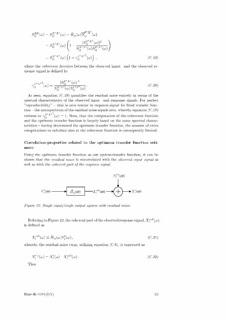
^ (w) - ' (o

= 1-1^ k)

4"^M (i-^'w), (C.19)

where the coherence function between the observed input- and the observed re­sponse signal is defined by

M (C.20)

As seen, equation (C.19) quantifies the residual noise entirely in terms of the spectral characteristics of the observed input- and response signals. For perfect ” reproducibility” - that is zero scatter in response signal for fixed transfer func­tion - the autospectrum of the residual noise equals zero, whereby equation (C.19) reduces to "Y^xt (iv) = 1. Note, that the computation of the coherence function and the optimum transfer function is largely based on the same spectral charac­teristics - having determined the optimum transfer function, the amount of extra computations to calculate also at the coherence function is consequently limited.

Correlation-properties related to the optimum transfer function esti­mate

Using the optimum transfer function as our system-transfer function, it can be shown that the residual noise is uncorrelated with the observed input signal as well as with the coherent part of the response signal.

Figure 22. Fing/e-inpui/sing/e-ou/pui sgs/em wi//?. residua/ noise.

Referring to Figure 22, the coherent part of the observed response signal, Xfoh(uj), is defined as

= (c.2i)

whereby the residual noise term, utilizing equation (C.6), is expressed as

(C.22)

Thus

Ris0-R-1181(EN) 55

^**(w) limT ——tt

limT ——tt

S F *XSij

c F lXSij

T T—tt T

* (w) - (w)Sf*F* (w)=0, (C.23)

which proves that the residual noise is uncorrelated with the observed input signal. To prove that the residual noise is uncorrelated with the coherent part of the response signal, simply note, from equation (C.21), that the coherent part of the response signal is given as a (constant) transfer function multiplied by the observed input signal. Thereby

SX ^°"^(w) ^lim

WijH limT—tt T

= =0,

where equation (C.23) has been utilized.

(C.24)

Characteristics of the optimum transfer function estimate

The last subject of interest, related to the choice of the optimum transfer functionestimate, is how this estimate compares with the ideal transfer function that cor­responds to the real physical quantities, where the noise contributions are absent. Let us consider the optimum transfer function, as expressed in equation (C.18), and let us elaborate a little on the quantities entering this expression.

Introducing equation (C.4), the numerator is expressed by

S F X* (w) ^lim H) (XjH + Ar;H)>

cfX(w) + cf"* (w) + c"'X (w) + c"' "* (w) (C.25)

Analogously, introducing equation (C.4) the denominator is expressed by

cF *F * (w) ^lim H) + Ar/M)>

SfF(w) + Sf"' (w) + S"'F(w) + S"'"' (w). (C.26)

Under the present experimental conditions, Fi(w) is associated with a determin­istic signal (the force established by the hammer hit). The ensemble averaging isespecially simple for deterministic signals, as

cF"= (w) ^im F.M^lim

Now, a characteristic for a noise signal is a zero mean. Thus

(C.27)

(t)) =°, (C.28)

56 Ris0-R-1181(EN)

which, due to the linearity of the ensemble mean operator, as well as of the Fouriertransform operator, is equivalent with

(#;(w))=0. (C.29)

Introducing equation (C.29) into equation (C.27) yields

Sf"* (w)=0. (C.30)

Referring to Figure 21 it is easily seen that Xi(w) is associated with a determin­istic signal when Fi(w) is associated with a deterministic signal. It is thus straight forward, by considerations analog to those for Sf" (w), to show that

S"'X (w)=0,

Sf"' (w)=0, (C.31)

Sj'F (w)=0.

If further, the noise associated with the observed input signal is assumed un­correlated with the noise associated with the observed response signal, then thefollowing relation holds

S"'" * (w)=0. (C.32)

Introducing equations (C.30)-(C.32) into equations (C.25)-(C.26) we obtain

Sij*X*(w) = SfX(w),

Sj *F * (w) = SgF(w)+Sj'"' (w)(C.33)

Combining equations (C.33) with equation (C.18) we finally arrive at the fol­lowing relationship between the ideal system transfer function and the estimated transfer function

#ij(w)1 + Sjf "'(w)

a^(w)(C.34)

Thus, for a situation with non-correlated extraneous input- and response noise, the optimum transfer function estimate, as based on observed quantities, is a biased estimate of the ideal transfer function. The inherent bias, in the estimated transfer function, depends on the input signal/noise ratio only, and tends consistently to zero for this noise contribution approaching zero.

If, instead of the present deterministic transient hammer excitation, an exci­tation technique based on continuous excitation with a random character forcing was applied, then an expression identical to equation (C.34), for the estimated optimum transfer function, is achieved, provided that the noise, superimposed on the response signal, is uncorrelated with the ideal input signal (meaning that Sf" (w) = 0), ansi that the noise, superimposed on the ideal input signal, is un­correlated with the ideal input signal (Sf" (w) = S"ff(w) = 0) as well as with the ideal response signal (S jX (w) = 0)

As seen from equation (C.19), the coherence function quantifies the amount of scatter in the results introduced by the presence of extraneous noise sources in the observed signals. Computing the coherence between observed input- and output

Ris0-R-1181(EN) 57

signals, according to equation (C.20), we shall now see how this function reflects the extraneous noise sources as described by equations (C.2) and (C.3). We adoptthe same assumptions as introduced in the treatment of the optimum transferfunction estimate, and equation (C.33) thus still applies, whereby

|Sj*X*(w)|2 = |SgX(w)|2 .

Moreover, equation (C.25) reduces to

(C.35)

Sj*F* (w) = SgF(w) + Sj'"' (w),

and finally the (observed) response autospectrum is reduced to

(C.36)

SX*X*Sij (w) lim -( + +T—tt TV /

SXX(w)+SX"* (w)+S" *X (w)+Sj *" * (w)

SXX(w)+Sj*"*(w), (C.37)

where, for the last identity (if random excitation is applied), the presumptions have been extended to also include no correlation between the ideal response signal and the imposed noise on the response signal (SXN* (w) = SjX (w) = 0). The resulting expression for the coherence is obtained by introducing equations (C.35)- (C.37) into equation (C.20)

*X*2ij (w)|SfX(w

(SgF(w) + S"'"'(w^ (SgX(w) + Sj*"*(w))

____________________________

^ J ^ + ^(w) Jl

1 + 'srsiu) t1 +

2

(C.38)

as the coherence between the ideal signals (cf. equation (C.19)) is identical 1 for linear systems. The deviation from the ideal value (i.e. 1) of the coherence functionis thus due to the presence of extraneous noise on the input signal as well as on the response signal. The resulting coherence function depends explicitly on the signal/noise ratios related to both the input signal and the response signal. Note,that it is not possible to separate the integrated effect of the extraneous noise intothe involved noise components, based on computation of the coherence function,unless one of the noise sources is explicitly known a priori.

58 Ris0-R-1181(EN)

D Uncertainty in spectral estimates

The (expected) spectral quantities introduced in Appendix C are defined in terms if an ideal ensemble averaging procedure. However, the concept of ensemble av­eraging is an abstraction, which in practice is replaced by an averaging over a finite number of observations displaced in time, assuming that the stochastic pro­cess in question (noise, random excitation and corresponding random response, etc.) is a stationary and ergodic process. In addition to the uncertainty caused by natural variability of the observed forcing- and response signals, as dealt with in Appendix C, the estimation of the (expected) associated cross- and autospectra consequently further introduces statistical uncertainty.

The dependence of the statistical uncertainty on the number of observations (on which the performed averaging procedure is based) is addressed in the following, assuming only that the available observations are statistical independent.

Let us, as an example, focus on the evaluation of the cross spectrum between the observed forcing (applied in DOF number i) and the observed response (at DOF number j). According to the definition given in equation (C.12), we have

^ ^lim . (D.l)

In practice the limiting process, included in definition above, is omitted, and asuitable (fixed) size of the observation time T is selected, reflecting the required lower cut-off frequency. This approximation does not affect the statistical uncer­tainty on the estimates, but relates only to the available frequency range. Thus, in practice, the definition given in equation (D.1) is replaced by

AX*F *Sij (w)2

(D.2)

where the spectral estimate is denoted by SXtFt (w), and the mean value estimate

operator M[•] is defined by

MN

"Z (7‘hf-h)l=1

1 (D.3)

where N denotes the number of (statistical independent) recordings. The necessary total recording time is then at least NT .

Let Xi(uj)Fj(uj) follow some (arbitrary) probability function with mean value jraw and variance a2raw. Denoting a ”true” mean value operator by E[-], the random error on the spectral estimate (D.2), expressed in terms of the variance of the spectral estimate, o (w)r, is given by

ogx*F* (w)2 — E AX*F *Sij (w) - E SXF (w)2

(D.4)

Utilizing equations (D.2) and (D.3), the second term in equation (D.4) can be reformulated as

Ris0-R-1181(EN) 59

E SX ^ (w) E

= ne

l=1

9 N

l = 1

1 2 NT

"E^1=1

_ 1 2 .. _ 2— N y^Mraui — rp^raw ■

Introducing equation (D.5) in equation (D.4) yields

(D.5)

o gx*F* (w)2 — E

-^E"

N

"

l=1 l=1

— _L J EE2 AT2 |

E ((%;(w)E«M)^ -j ^E ((%;MEj(w))^ -j j.(D.6)

When, as assumed, ^Xi(w)Ej(w)j are statistical independent quantities, thefollowing holds

E (E ̂J f E ^" "

l = 1 m=1""

El = 1 m=1"

El=1"

— Y O

$lm ( ( X ^Uj) Fj (ivYj i — flr aw J i(^) Fj (o>)J ~ flraw

— Z^ratu

^ , Oraw Noraw J (D.7)l=1

where the linearity of the operator E[•] has been been utilized and Slm is the Kronecker delta. Introducing equation (D.7) into equation (D.6) finally yields

z \2 41 2(Tgxtft M - 7^2 ^rotu , (D.8)

where N = 1 corresponds to the spectral raw estimate.Equation (D.8) shows, that the statistical uncertainty on the estimate of the

cross spectrum is inversely proportional to the number of averages used in the estimation, and further that this random error tend to zero for the number of

2

2

2

2

60 Ris0-R-1181(EN)

averages approaching infinitely (as expected). In practice, usually only a limited number of averages is necessary to obtain sufficient accuracy (say, of the order of 5).

Analog results for estimates of autospectra are easily derived from the above derivation by replacing with or

Ris0-R-1181(EN) 61

62 Ris0-R-1181(EN)

E Alternative experimental strate­gies

Different alternative experimental strategies have been investigated during thecourse of the project in order to establish the most suitable experimental procedurefor wind turbine blade testing. These are briefly accounted for in the present appendix.

Apart from the impact excitation concept, accounted for in Chapter 3, two alternative exitation principles have been considered - snap back excitation and random exitation using an electromagnetic exciter. In addition, different analysis strategies were associated with each of these approaches.

E.1 Snap-Back ExperimentsIn snap-back experiments the structure is elastically deformed and then instan­taneously released - the structure snaps back. Depending on the contribution of the individual mode shapes to the initial structural deflection of the blade (and possible non-linearities in the structure), the derived free oscillations contain a range of mode shapes, each vibrating with their respective natural frequencies.

Experimental procedure

One end of a fishing line, with an adequate breaking strength, was attached to the blade - the other end was, through a force transducer, attached to a winch. The winch was subsequently pulled so that the blade was conveniently deflected, until the fishing line finally fails, and the blade snapped back. The associated jump in the measured force was used to trigger the measurements.

The motion of the blade was measured using two reference accelerometers lo­cated at the blade tip, and three accelerometers mounted on the conventional measuring bridge (cf. Figure 4) at the cross section in question.

The measurements were repeated with the three accelerometers, resolving flapwise-, edgewise- and torsional deflection, placed in 10 different cross section.

Analysis procedure

The applied analysis method differ from the one described in Chapter 3. As no forcing is recorded, the analysis can not be based on the concept of transfer func­tions. Instead, the analysis is performed in the time domain, using the reference measurement to link the modal decompositions originating from different cross sections.

Using the algorithm described in Appendix A to relate cross sectional DOF’s with cross sectional displacements, the basic idea is to express a measured response in terms of a modal expansion as formulated in equation (7). The modal expansion is truncated by selecting a suitable number of relevant mode shapes. Each term in the truncated modal expansion contains a modal amplitude, a modal damping factor (essentially the real part of the eigenvalues associated with the eigenvalue problem (3)), and a natural frequency (the imaginary part of the eigenvalues as­sociated with the eigenvalue problem (3)). As the modal amplitudes are complex quantities, accounting for weightning of the individual modes as well as mutual phase shift between these, we are left with 4 parameters for each contributing mode to be determined. These are determined numerically by means of a opti­mization procedure based on the least square principle. The optimization aims at

Ris0-R-1181(EN) 63

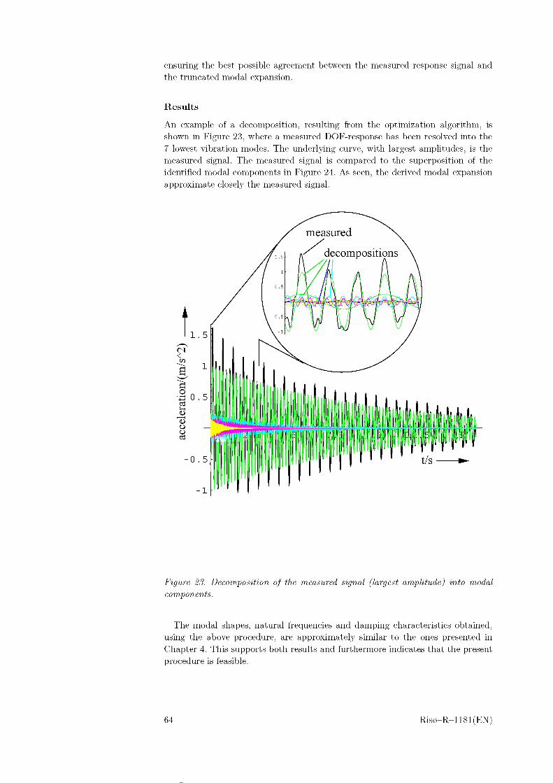
ensuring the best possible agreement between the measured response signal and the truncated modal expansion.

Results

An example of a decomposition, resulting from the optimization algorithm, is shown in Figure 23, where a measured DOF-response has been resolved into the 7 lowest vibration modes. The underlying curve, with largest amplitudes, is the measured signal. The measured signal is compared to the superposition of the identified modal components in Figure 24. As seen, the derived modal expansion approximate closely the measured signal.

1.5

0.5

■0.5

1

1

I "ril

Figure 23. Decomposition of the measured signal (largest amplitude) into modal cmMpon.en.k.

The modal shapes, natural frequencies and damping characteristics obtained, using the above procedure, are approximately similar to the ones presented in Chapter 4. This supports both results and furthermore indicates that the present procedure is feasible.

64 Ris0-R-1181(EN)

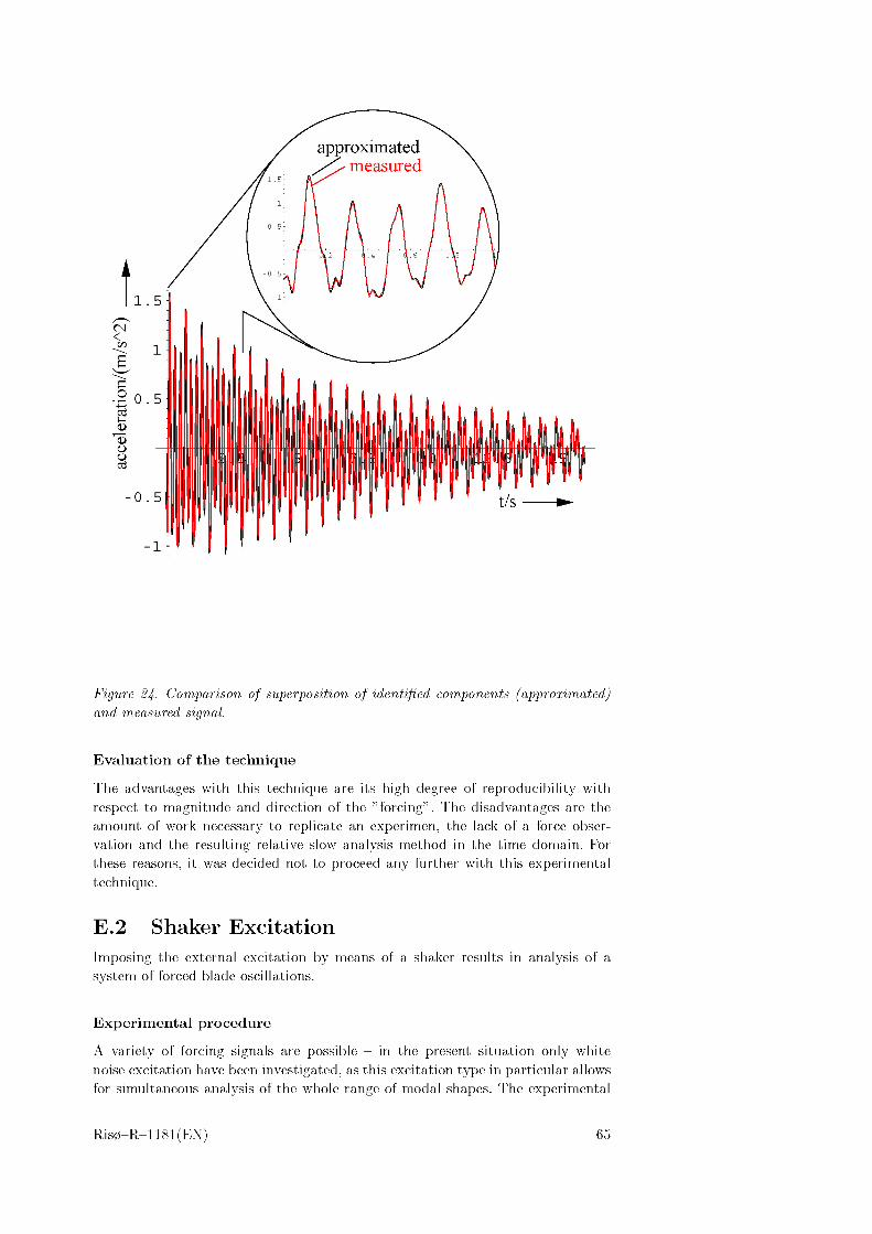
figure Comparison o/sapeTpos#ion o/ Wen^efZ cofnponents ^approrimaW^ and measured signed.

Evaluation of the technique

The advantages with this technique are its high degree of reproducibility with respect to magnitude and direction of the ” forcing”. The disadvantages are the amount of work necessary to replicate an experimen, the lack of a force obser­vation and the resulting relative slow analysis method in the time domain. For these reasons, it was decided not to proceed any further with this experimental technique.

E.2 Shaker ExcitationImposing the external excitation by means of a shaker results in analysis of a system of forced blade oscillations.

Experimental procedure

A variety of forcing signals are possible - in the present situation only white noise excitation have been investigated, as this excitation type in particular allows for simultaneous analysis of the whole range of modal shapes. The experimental

Ris0-R-1181(EN) 65

procedure is thus eased considerably compared e.g. to sinusoidal excitation.Recording simultaneously the external forcing and the derived response, the

experimental analysis can be performed in the frequency domain based on the transfer matrix (cf. Section 3.2). The analysis method is thus analogue to the one applied for the transient excitation.

Different types of exciters exist - hex. exiters based on an electromagnetic prin­ciple and hydraulic exiters. The exiter applied in the present experiments was an electromagnetic vibration exciter of the type B&K (Briiel &; Kjasr) 4808 (cf. Appendix F). In principle the shaker works, and is controlled, similar to a loud­speaker.

Due to the symmetry of the transfer matrix, expressing the dynamic relationship between excitation (direction, magnitude) at a given location and the structural response in one of the defined DOF’s, the experiment can be performed either with fixed excitation location and roving response recording, corresponding to the chosen discretization of the blade motion, or vice versa. Moving the exciter, and in particular the attachment of the exciter, along the blade is, however, some­what cumbersome. Therefore, the only practical way of performing this type of experiments is to have the excitation fixed. The experimental setup employed is illustrated in the pictures below.

66 Ris0-R-1181(BN)

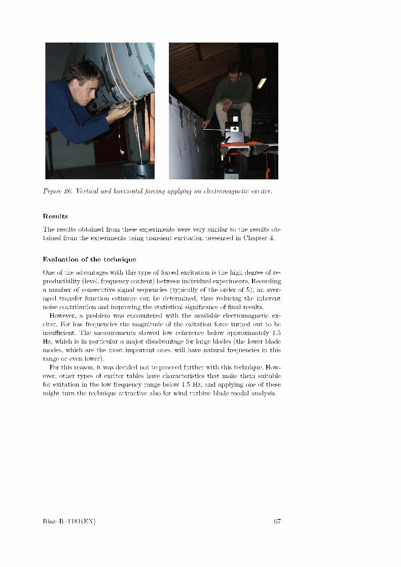
F%wre arzd /orcm# appf?/m^ arz e/ec^mma^Me^c eraser.

Results

The results obtained from these experiments were very similar to the results ob­tained from the experiments using transient excitation presented in Chapter 4.

Evaluation of the technique

One of the advantages with this type of forced excitation is the high degree of re­producibility (level, frequency content) between individual experiments. Recording a number of consecutive signal sequencies (typically of the order of 5), an aver­aged transfer function estimate can be determined, thus reducing the inherent noise contribution and improving the statistical significance of final results.

However, a problem was encountered with the available electromagnetic ex­citer. For low frequencies the magnitude of the exitation force turned out to be insufficient. The measurements showed low coherence below approximately 1.5 Hz, which is in particular a major disadvantage for large blades (the lower blade modes, which are the most important ones, will have natural frequencies in this range or even lower).

For this reason, it was decided not to proceed further with this technique. How­ever, other types of exciter tables have characteristics that make them suitable for exitation in the low frequency range below 1.5 Hz, and applying one of these might turn the technique attractive also for wind turbine blade modal analysis.

Ris0-R-1181(EN) 67

68 Ris0-R-1181(EN)

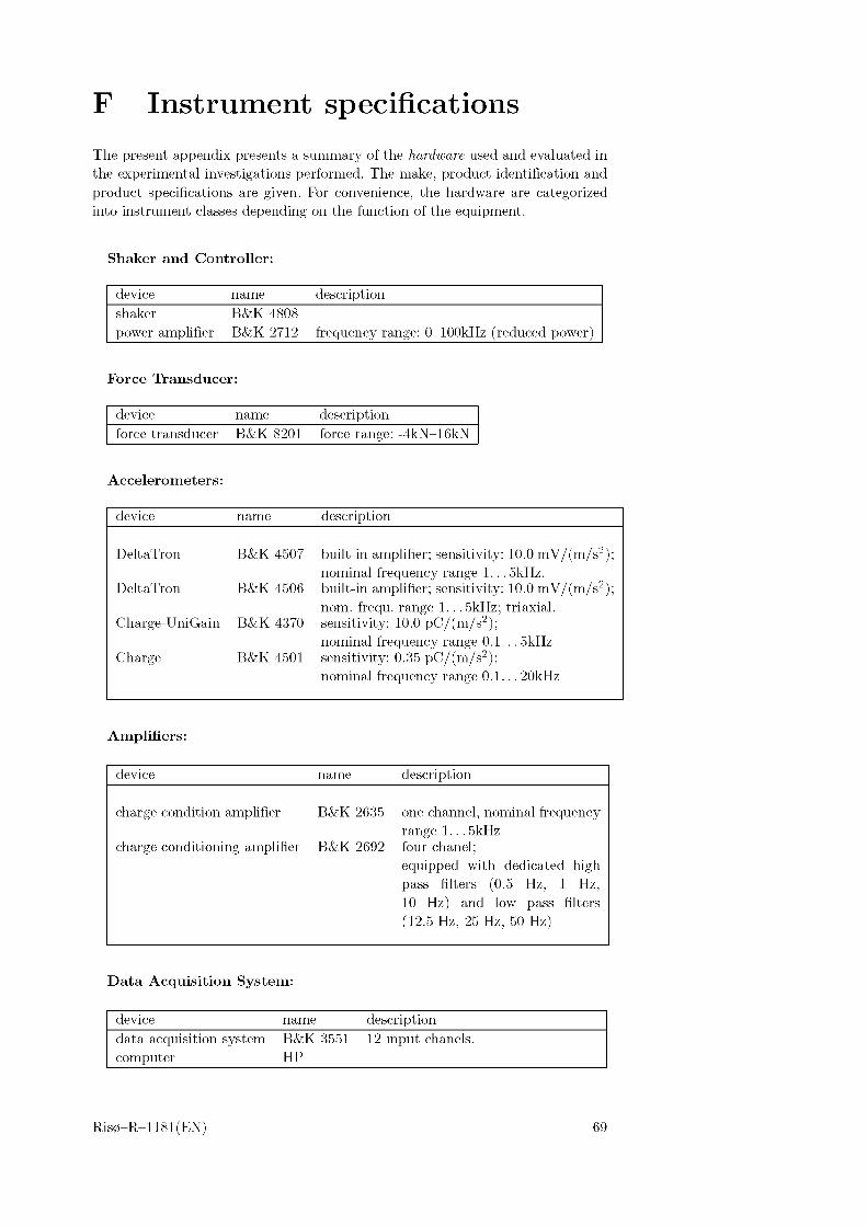
F Instrument specifications

The present appendix presents a summary of the hardware used and evaluated inthe experimental investigations performed. The make, product identification and product specifications are given. For convenience, the hardware are categorizedinto instrument classes depending on the function of the equipment.

Shaker and Controller:

device name descriptionshakerpower amplifier

B&K 4808 B&K 2712 frequency range: O-lOOkHz (reduced power)

Force Transducer:

device name descriptionforce transducer B&K 8201 force range: -4kN-16kN

Accelerometers:

device name description

DeltaTron B&K 4507 built-in amplifier; sensitivity: 10.0 mV/(m/s2); nominal frequency range 1... 5kHz.

DeltaTron B&K 4506 built-in amplifier; sensitivity: 10.0 mV/(m/s2); nom. frequ. range 1... 5kHz; triaxial.

Charge-UniGain B&K 4370 sensitivity: 10.0 pC/(m/s2); nominal frequency range 0.1... 5kHz

Charge B&K 4501 sensitivity: 0.35 pC/(m/s2); nominal frequency range 0.1... 20kHz

Amplifiers:

device name description

charge condition amplifier

charge conditioning amplifier

B&K 2635

B&K 2692

one channel; nominal frequency range 1... 5kHz four chanel;equipped with dedicated high pass filters (0.5 Hz, 1 Hz, 10 Hz) and low pass filters (12.5 Hz, 25 Hz, 50 Hz)

Data Acquisition System:

device name descriptiondata acquisition system computer

B&K 3551 HP

12 input chanels.

Ris0-R-1181(EN) 69

70 Ris0-R-1181(EN)

G FEM Model

The FE modeling of the blade is due to M.L. Th0gersen and J.T. Petersen, Ris0 [6]. The blade structure properties have been approached by neglecting the elastic­ity (but not the weight) of the tip brake mechanism and by assuming the root part to be fully clamped (and thus neglecting the moderate elasticity of the support structure). Moreover, the material damping properties are not taken into account.

Basically, the blade model is a shell model. The surface geometry is defined by connecting a number of predefined blade cross sections with radial splines. The geometry of webs and other inner support structures is defined by subsequently connecting suitable surface points with area elements. The defined surface area is subsequently subdivided into 8-nodes triangular shell elements with quadratic in­terpolation functions. The element is capable of modeling 100 layers of ortotropic material properties, but only one layer, representing the average properties over the shell thickness, was applied in the present modeling. Within a particular el­ement the material properties are considered isotropic. The model has 4000 ele­ments, 6000 nodes and 36000 DOF’s.

Ris0-R-1181(EN) 71

Title and author(s)Modal Analysis of Wind Turbine Blades

Bibliographic Data Sheet Ris0—R—1181(EN)

Gunner C. Larsen, Morten H. Hansen, Andreas Baumgart, Ingemar Carlen

ISBN87-550-2696-6; 87-550-2697-4 (Internet)

ISSN0106-2840

Dept. or group DateAED/VEA February 2002

Groups own reg. number(s) Project/contract No.1120098 ENS-1363/98-0010

Pages Tables Illustrations References71 8 26 16Abstract (Max. 2000 char.)The modal analysis technique has been used to identify essential dynamic proper­ties of wind turbine blades like natural frequencies, damping characteristics and mode shapes.Different experimental procedures have been considered, and the most appropriate of these has been selected. Although the comparison is based on measurements on a LM 19 m blade, the recommendations given are believed to be valid for otherwind turbine blades as well.The reliability of the selected experimental analysis has been quantified by es­timating the unsystematic variations in the experimental findings. Satisfactory results have been obtained for natural frequencies, damping characteristics andfor the dominating deflection direction of the investigated mode shapes. For the ’’secondary” deflection directions, the observed experimental uncertainty may be considerable - especially for the torsional deflection.The experimental analysis of the LM 19 m blade has been compared with results from a state-of-the-art FE-modeling of the same blade. For some of the higher modes substantial discrepancies between the natural frequencies originating from the FE-modeling and the modal analysis, respectively, are observed. In general the qualitative features of measured and computed modes shapes are in good agree­ment. However, for the ” secondary” deflection directions, substantial deviations in the absolute values may occur (when normalizing with respect to the primary deflection direction).Finally, suggestions of potential future improvements of the experimental proce­dure are discussed.

Descriptors INIS/EDBDYNAMIC LOADS; ELASTICITY; MECHANICAL VIBRATIONS; NONDE­STRUCTIVE TESTING; RESPONSE FUNCTIONS; STRUCTURAL MODELS; TURBINE BLADES; WIND TURBINES