HAL Id: hal-00750909https://hal.archives-ouvertes.fr/hal-00750909

Submitted on 12 Nov 2012

HAL is a multi-disciplinary open accessarchive for the deposit and dissemination of sci-entific research documents, whether they are pub-lished or not. The documents may come fromteaching and research institutions in France orabroad, or from public or private research centers.

L’archive ouverte pluridisciplinaire HAL, estdestinée au dépôt et à la diffusion de documentsscientifiques de niveau recherche, publiés ou non,émanant des établissements d’enseignement et derecherche français ou étrangers, des laboratoirespublics ou privés.

Distributed under a Creative Commons ttributionttribution 4.0 International License

Model-Based Clustering of High-Dimensional Data: Areview

Charles Bouveyron, Camille Brunet

To cite this version:Charles Bouveyron, Camille Brunet. Model-Based Clustering of High-Dimensional Data:A review. Computational Statistics and Data Analysis, Elsevier, 2013, 71, pp.52-78.<10.1016/j.csda.2012.12.008>. <hal-00750909>

Bou

veyro

n&

Bru

net

–D

raft

Ver

sion

ofN

ovem

ber

12,

2012

–U

niv

ersi

téP

aris

1

Model-Based Clustering of High-Dimensional Data : A review

Charles Bouveyron∗ & Camille Brunet†1

∗ Laboratoire SAMM, EA 4543

Université Paris 1 Panthéon-Sorbonne

† Laboratoire LAREMA, UMR CNRS 6093

Université d’Angers

Abstract

Model-based clustering is a popular tool which is renowned for its probabilistic foundations

and its flexibility. However, high-dimensional data are nowadays more and more frequent

and, unfortunately, classical model-based clustering techniques show a disappointing be-

havior in high-dimensional spaces. This is mainly due to the fact that model-based cluster-

ing methods are dramatically over-parametrized in this case. However, high-dimensional

spaces have specific characteristics which are useful for clustering and recent techniques

exploit those characteristics. After having recalled the bases of model-based clustering,

this article will review dimension reduction approaches, regularization-based techniques,

parsimonious modeling, subspace clustering methods and clustering methods based on

variable selection. Existing softwares for model-based clustering of high-dimensional data

will be also reviewed and their practical use will be illustrated on real-world data sets.

Keywords: Model-based clustering, high-dimensional data, dimension reduction,

regularization, parsimonious models, subspace clustering, variable selection, softwares,

R packages.

1. Introduction

Clustering is a data analysis tool which aims to group data into several homoge-

neous groups. The clustering problem has been studied for years and usually occurs in

applications for which a partition of the data is necessary. In particular, more and more

scientific fields require to cluster data in the aim to understand or interpret the studied

phenomenon. Earliest approaches were based on heuristic or geometric procedures. They

relied on dissimilarity measures between pairs of observations. A popular dissimilarity

measure is based on the distance between groups, previously introduced by Ward [97] for

hierarchical clustering. In the same way, the k-means algorithm [55] is perhaps the most

popular clustering algorithm among the geometric procedures. Clustering was also defined

in a probabilistic framework, allowing to formalize the notion of clusters through their

probability distribution. One of the main advantages of this probabilistic approach is in

the fact that the obtained partition can be interpreted from a statistical point of view. The

Preprint submitted to Elsevier November 12, 2012

Bou

veyro

n&

Bru

net

–D

raft

Ver

sion

ofN

ovem

ber

12,

2012

–U

niv

ersi

téP

aris

1

first works on finite mixture models were from Wolfe [99], Scott et al. [87] and Duda et

al. [29]. Since then, these models have been extensively studied and, thanks to works such

as those of McLachlan et al. [62, 64], Banfield & Raftery [5] or Fraley & Raftery [33],[35],

model-based clustering has become a popular and reference technique.

Nowadays, the measured observations in many scientific domains are frequently high-

dimensional and clustering such data is a challenging problem for model-based methods.

Indeed, model-based methods show a disappointing behavior in high-dimensional spaces.

They suffer from the well-known curse of dimensionality [6] which is mainly due to the fact

that model-based clustering methods are over-parametrized in high-dimensional spaces.

Furthermore, in several applications, such as mass spectrometry or genomics, the num-

ber of available observations is small compared to the number of variables and such a

situation increases the problem difficulty. Since the dimension of observed data is usually

higher than their intrinsic dimension, it is theoretically possible to reduce the dimension of

the original space without loosing any information. For this reason, dimension reduction

methods are frequently used in practice to reduce the dimension of the data before the

clustering step. Feature extraction methods, such as principal component analysis (PCA),

or feature selection methods are very popular. However, dimension reduction usually does

not consider the classification task and provide a sub-optimal data representation for the

clustering step. Indeed, dimension reduction methods imply an information loss which

could have been discriminative.

To avoid the drawbacks of dimension reduction, several approaches have been proposed

to allow model-based methods to efficiently cluster high-dimensional data. This work pro-

poses to review the alternatives to dimension reduction for dealing with high-dimensional

data in the context of model-based clustering. Earliest approaches include constrained and

parsimonious models or regularization. More recently, subspace clustering techniques and

variable selection techniques have been proposed to overcome the limitations of previous

approaches. Subspace clustering techniques are based on probabilistic versions of the fac-

tor analysis model. This modeling allows to cluster the data in low-dimensional subspaces

without reducing the dimension. Conversely, variable selection techniques do reduce the

dimension of the data but select the variables to retain regarding the clustering task. Both

techniques turn out to be very efficient and their practical use will be discussed as well in

this article.

This article is organized as follows. Section 2 briefly recalls the bases of mixture model-

ing and its inference with the EM algorithm. Section 3 introduces the curse of dimension-

ality in model-based clustering. Approaches based on dimension reduction, regularization

and parsimonious models are reviewed in Section 4. Then, Section 5 and 6 present re-

spectively the approaches based on subspace clustering and variable selection. Existing

softwares for model-based clustering of high-dimensional data are also reviewed in Sec-

tion 7 and their practical use is discussed in Section 8. Finally, some concluding remarks

are made in Section 9.

2

Bou

veyro

n&

Bru

net

–D

raft

Ver

sion

ofN

ovem

ber

12,

2012

–U

niv

ersi

téP

aris

1

2. The mixture model and the EM algorithm

This section first recalls the bases of mixture modeling and its inference with the

expectation-maximization (EM) algorithm.

2.1. The mixture model

Let us consider a data set of n observations y1, . . . , yn ∈ Rp that one wants to divide

into K homogeneous groups. The aim of clustering is to determine, for each observation

yi, the value of its unobserved label zi such that zi = k if the observation yi belongs to

the kth cluster. To do so, model-based clustering [35, 64] considers the overall population

as a mixture of the groups and each component of this mixture is modeled through its

conditional probability distribution. In this context, the observations y1, . . . , yn ∈ Rp

are assumed to be independent realizations of a random vector Y ∈ Rp whereas the

unobserved labels z1, ..., zn are assumed to be independent realizations of a random

variable Z ∈ 1, ...,K. The set of pairs (yi, zi)ni=1 is usually referred to as the complete

data set. By denoting by g the probabilistic density function of Y , the finite mixture model

is:

g(y) =K∑

k=1

πkfk(y), (1)

where πk (with the constraint∑K

k=1 πk = 1) and fk respectively represent the mixture

proportion and the conditional density function of the kth mixture component. Further-

more, the clusters are often modeled by the same parametric density function in which

case the finite mixture model is:

g(y) =K∑

k=1

πkf(y; θk), (2)

where θk is the parameter vector for the kth mixture component. For a set of observations

y = y1, ..., yn, the log-likelihood of this mixture model is then:

ℓ (θ; y) =n∑

i=1

log

(

K∑

k=1

πkf (yi; θk)

)

. (3)

However, the inference of this model cannot be directly done through the maximization of

the likelihood since the group labels z1, ..., zn of the observations are unknown. Indeed,

due to the exponential number of solutions to explore, the maximization of equation (3)

is unfortunately intractable, even for limited numbers of observations and groups. Before

introducing the most popular inference algorithm used in this context, let us introduce

the complete log-likelihood:

ℓc(θ; y, z) =n∑

i=1

K∑

k=1

zik log (πkf (yi; θk)) ,

where zik = 1 if the ith observation belongs to the kth cluster and zik = 0 otherwise.

3

Bou

veyro

n&

Bru

net

–D

raft

Ver

sion

ofN

ovem

ber

12,

2012

–U

niv

ersi

téP

aris

1

2.2. The EM algorithm

Although it is not specifically dedicated to mixture models, the expectation-maximization

(EM) algorithm, proposed by Dempster et al. [28], is certainly the most popular technique

for inferring mixture models. The EM algorithm iteratively maximizes the conditional

expectation of the complete log-likelihood:

E [ℓc (θ; y, z) |θ∗] =K∑

k=1

n∑

i=1

tik log (πkf (yi; θk)) ,

where tik = E [z = k|yi, θ∗] and θ∗ is a given set of the mixture parameters. From an initial

solution θ(0), the EM algorithm alternates two steps: the E-step and the M-step. First,

the expectation step (E-step) computes the expectation of the complete log-likelihood

E[

ℓc (θ; y, z) |θ(q)]

conditionally to the current value of the parameter set θ(q). Then, the

maximization step (M-step) maximizes E[

ℓc (θ; y, z) |θ(q)]

over θ to provide an update for

the parameter set. This algorithm therefore forms a sequence(

θ(q))

q≥1which satisfies, for

each q ≥ 1:

θ(q+1) = arg maxθ

E[

ℓc (θ; y, z) |θ(q)]

.

One of the most outstanding properties of the EM algorithm is that it guarantees an

improvement of the likelihood function at each iteration. Each update of the parameter set,

resulting from an E-step followed by an M-step, is guaranteed to increase the log-likelihood

function. In particular, Wu [100] proved that the sequence of(

θ(q))

q≥1converges to a local

optimum of the likelihood. For further details on the EM algorithm, the reader may refer

to [63].

The two steps of the EM algorithm are iteratively applied until a stopping criterion

is satisfied. The stopping criterion may be simply |ℓ(θ(q); y) − ℓ(θ(q−1); y)| < ε where ε

is a positive value to provide. It would be also possible to use the Aitken’s acceleration

criterion [53] which estimates the asymptotic maximum of the likelihood and allows to

detect in advance the algorithm convergence. Once the EM algorithm has converged,

the partition z1, . . . , zK of the data can be deduced from the posterior probabilities

tik = P (Z = k|yi, θ) by using the maximum a posteriori (MAP) rule which assigns the

observation yi to the group with the highest posterior probability.

2.3. The Gaussian mixture model

Among the possible probability distributions for the mixture components, the Gaussian

distribution is certainly the most used for both theoretical and computational reasons. Let

us however notice that several recent works focused on different distributions such as the

skew normal [52], asymmetric Laplace [36] or t-distributions [3, 51, 68]. Nevertheless, the

density function f(y; θk) is most commonly assumed to be a multivariate Gaussian density

φ(y; θk) parametrized by its mean µk and its covariance matrix Σk, such that the density

4

Bou

veyro

n&

Bru

net

–D

raft

Ver

sion

ofN

ovem

ber

12,

2012

–U

niv

ersi

téP

aris

1

function of Y can be written as:

g(y; θ) =K∑

k=1

πkφ(y; θk), (4)

where:

φ(y; θk) =1

(2π)p/2 |Σk|1/2exp

(

−1

2(y − µk)t Σ−1

k (y − µk)

)

is the multivariate Gaussian density with parameter θk = (µk,Σk). This specific mixture

model is usually referred in the literature as the Gaussian mixture model (GMM). In this

case, the EM algorithm has the following form, at iteration q:

E-step. This step aims to compute the expectation of the complete log-likelihood condi-

tionally to the current value of the parameter θ(q−1). In practice, it reduces to the com-

putation of t(q)ik = E[zi = k|yi, θ

(q−1)]. Let us also recall that t(q)ik is as well the posterior

probability P (zi = k|yi, θ(q−1)) that the observation yi belongs to the kth component of

the mixture under the current model. Using Bayes’ theorem, the posterior probabilities

t(q)ik , i = 1, ..., n, k = 1, ...,K, can be expressed as follows:

t(q)ik =

π(q−1)k φ(yi, θ

(q−1)k )

∑Kl=1 π

(q−1)l φ(yi|θ

(q−1)l )

, (5)

where π(q−1)k and θ

(q−1)k =

µ(q−1)k ,Σ

(q−1)k

are the parameters of the kth mixture compo-

nent estimated at the previous iteration.

M-step. This step updates the model parameters by maximizing the conditional expecta-

tion of the complete log-likelihood. The maximization of E[

ℓc (θ; y, z) |θ(q−1)]

conduces to

an update of the mixture proportions πk, the means µk and the covariance matrices Σk as

follows, for k = 1, ...,K:

π(q)k =

n(q)k

n, (6)

µ(q)k =

1

n(q)k

n∑

i=1

t(q)ik yi, (7)

Σ(q)k =

1

n(q)k

n∑

i=1

t(q)ik

(

yi − µ(q)k

) (

yi − µ(q)k

)t, (8)

where n(q)k =

∑ni=1 t

(q)ik .

3. The curse of dimensionality in model-based clustering

Before to present classical and recent methods for high-dimensional data clustering, we

focus in this section on the causes of the curse of dimensionality in model-based clustering.

5

Bou

veyro

n&

Bru

net

–D

raft

Ver

sion

ofN

ovem

ber

12,

2012

–U

niv

ersi

téP

aris

1

3.1. The origins: the Bellman’ sentence

When reading research articles or books related to high-dimensional data, it is very

likely to find the term “curse of dimensionality” to refer to all problems caused by the

analysis of high-dimensional data. This term was introduced by R. Bellman in the preface

of his book [6] promoting dynamic programming. To illustrate the difficulty to work in

high-dimensional spaces, Bellman recalled that if one considers a regular grid with step 0.1

on the unit cube in a 10-dimensional space, the grid is made of 1010 points. Consequently,

the search for the optimum of a given function in this unit cube requires 1010 evaluations

of this function which was unfordable problem in the 60’s (it remains a difficult problem

nowadays). Although the term “curse of dimensionality” used by Bellman is of course

rather pessimistic, the paragraph of the preface in which the term first appeared is in fact

more optimistic:

All this [the problems linked to high dimension] may be subsumed under

the heading « the curse of dimensionality ». Since this is a curse, [...], there is

no need to feel discouraged about the possibility of obtaining significant results

despite it.

This paragraph will indeed show that the Bellman’s thought was corrected since, at least

for clustering, high dimensions have nice properties which do allow to obtain significant

results.

3.2. The curse of dimensionality in model-based clustering

In the context of model-based clustering, the curse of dimensionality takes a particular

form. Indeed, model-based clustering methods require the estimation of a number of pa-

rameters which directly depends on the dimension of the observed space. If we consider the

classical Gaussian mixture model for instance, the total number of parameters to estimate

is equal to:

ν = (K − 1) +Kp+Kp(p− 1)/2,

where (K − 1), Kp and Kp(p − 1)/2 are respectively the numbers of free parameters for

the proportions, the means and the covariance matrices. It turns out that the number of

parameters to estimate is therefore a quadratic function of p in the case of the Gaussian

mixture model and a large number of observations will be necessary to correctly estimate

those model parameters. Furthermore, a more serious problem occurs in the EM algorithm

when computing the posterior probabilities tik = E[Z = k|yi, θ] which depend, in the

GMM context, on the quantity Hk(x) = −2 log(πkφ(x;µk,Σk)). Indeed, the computation

of Hk, which can be rewritten as:

Hk(x) = (x− µk)tΣ−1k (x− µk) + log(det Σk) − 2 log(πk) + p log(2π), (9)

requires the inversion of the covariance matrices Σk, k = 1, ...,K. Consequently, if the

number of observations n is small compared to ν, the estimated covariance matrices Σk

are ill-conditioned and their inversions conduce to unstable classification functions. In the

6

Bou

veyro

n&

Bru

net

–D

raft

Ver

sion

ofN

ovem

ber

12,

2012

–U

niv

ersi

téP

aris

1

worst case where n < p, the estimated covariance matrices Σk are singular and model-

based clustering methods cannot be used at all. Unfortunately, this kind of situation tends

to occur more and more frequently in Biology (DNA sequences, genotype analysis) or in

computer vision (face recognition) for instance.

The curse of dimensionality has been also exhibited by [80, 81] in the Gaussian case

with the estimation point of view. Let us consider the estimation of the normalized trace

τ(Σ) = tr(Σ−1)/p of the inverse covariance matrix Σ of a multivariate Gaussian distribu-

tion N (µ,Σ). The estimation of τ from a sample of n observations x1, ..., xn conduces

to:ˆτ(Σ) = τ(Σ) =

1

ptr(Σ−1),

and its expectation is:

E[ ˆτ(Σ)] =

(

1 −p

n− 1

)−1

τ(Σ).

Consequently, if the ratio p/n → 0 when n → +∞, then E[ ˆτ(Σ)] → τ(Σ). However,

if the dimension p is comparable with n, then E[ ˆτ(Σ)] → cτ(Σ) when n → +∞, where

c = limn→+∞ p/n. We refer to [80, 81] for further details on the effect of the dimensionality

on classification in the asymptotic framework, i.e. p and n → +∞.

3.3. The blessing of dimensionality in clustering

Hopefully, as expected by Bellman, high-dimensional spaces have specific features

which could facilitate their exploration. Several authors, such as [44, 75], have shown

that, in the context of clustering, high-dimensional spaces do have useful characteristics

which ease the classification of data in those spaces. In particular, Scott and Thompson

[88] showed that high-dimensional spaces are mostly empty. The experiment suggested

by Huber [47] consists in drawing realizations of a p-dimensional random vector X with

uniform probability distribution on the hypersphere of radius 1. The probability that a

realization xi of this experiment belongs to the shell between the hypersphere of radius

0.9 and the unit hypersphere is therefore:

P (xi ∈ S0.9(p)) = 1 − 0.9p.

In particular, the probability that xi belongs to the shell between the hypersphere of radius

0.9 and the unit hypersphere in a 20-dimensional space is roughly equals to 0.88. Therefore,

most of the realizations of the random vector X live near a p − 1 dimensional subspace

and the remaining of the space is mostly empty. This suggests that clustering methods

should model the groups in low-dimensional subspaces instead to model them in the whole

observation space. Furthermore, it seems reasonable to expect that different groups live

in different subspaces and this may be a useful property for discriminating the groups.

Subspace clustering methods, presented in Section 6, exploit this specific characteristic of

high-dimensional spaces.

7

Bou

veyro

n&

Bru

net

–D

raft

Ver

sion

ofN

ovem

ber

12,

2012

–U

niv

ersi

téP

aris

1

4. Earliest approaches

Earliest approaches to deal with the clustering of high-dimensional data can be split

into three families: dimension reduction methods, regularization methods and parsimo-

nious methods.

4.1. Dimension reduction

Approaches based on dimension reduction assume that the number p of measured vari-

ables is too large and, implicitly, that the data at hand live in a space of lower dimension,

let us say d < p. Once the data projected in a low-dimensional space, it is then possible to

apply the EM algorithm on the projected observations to obtain a partition of the original

data.

The most popular linear method used for dimension reduction is certainly principal

component analysis (PCA). It was introduced by Pearson [82] who defines PCA as a

linear projection that minimizes the average projection cost. Later, Hotelling [46] proposed

another definition for PCA which reduces the dimension of the data by keeping as much

as possible the variation of the data set. In other words, this method aims to find an

orthogonal projection of the data set in a low-dimensional linear subspace, such that the

variance of the projected data is maximum. This leads to the classical result where the

principal axes u1, ..., ud are the eigenvectors associated with the largest eigenvalues of the

empirical covariance matrix S of the data. Several decades after, Tipping and Bishop [91]

proposed a probabilistic view of PCA by assuming that the observations are independent

realizations of a random variable Y ∈ Rp which is linked to a latent variable X ∈ R

d

through the linear relation:

Y = ΛtX + ε.

It is further assume that X ∼ N (µ, Id) and ε ∼ N (0, σ2Ip), such that the marginal

distribution of Y is N (Λµ,ΛtΛ + σ2Ip). The estimation of the parameters µ, Λ and b by

maximum likelihood conduces in particular to estimate Λ by the eigenvectors associated

with the largest eigenvalues of the empirical covariance matrix S of the data.

Factor analysis (FA) is an other way to deal with dimension reduction. This approach

is as old as PCA since its origins are relative to Spearman [90] and there is an important

literature on this subject too (see for example [12, chap. 12]). The basic idea of factor

analysis is to both reduce the dimensionality of the space and to keep the observed covari-

ance structure of the data. It turns out that the probabilistic PCA (PPCA) model is in

fact a particular case of the factor analysis model. Indeed, the FA model makes the same

assumption as the PPCA model except regarding the distribution of ε which is assumed

to be N (0,Ψ), where Ψ is a diagonal covariance matrix. However, conversely to the PPCA

model, the estimation of model parameters by maximum likelihood does not conduce to

closed-form estimators.

8

Bou

veyro

n&

Bru

net

–D

raft

Ver

sion

ofN

ovem

ber

12,

2012

–U

niv

ersi

téP

aris

1

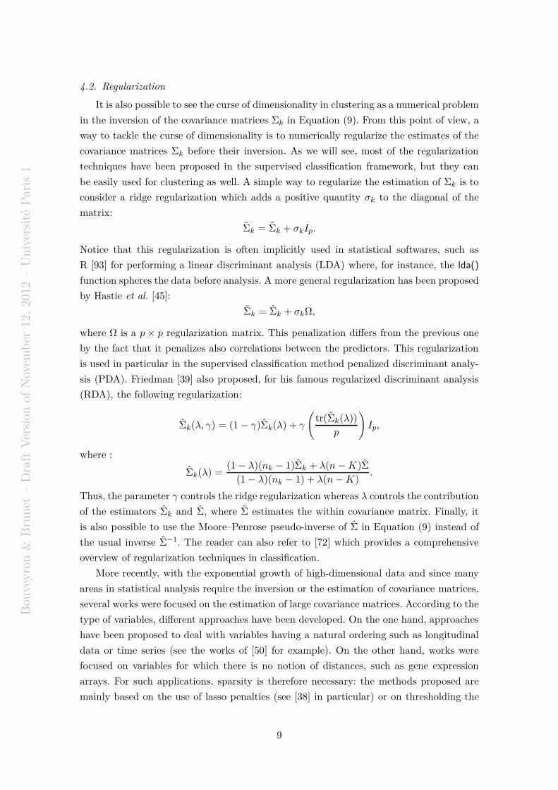
4.2. Regularization

It is also possible to see the curse of dimensionality in clustering as a numerical problem

in the inversion of the covariance matrices Σk in Equation (9). From this point of view, a

way to tackle the curse of dimensionality is to numerically regularize the estimates of the

covariance matrices Σk before their inversion. As we will see, most of the regularization

techniques have been proposed in the supervised classification framework, but they can

be easily used for clustering as well. A simple way to regularize the estimation of Σk is to

consider a ridge regularization which adds a positive quantity σk to the diagonal of the

matrix:

Σk = Σk + σkIp.

Notice that this regularization is often implicitly used in statistical softwares, such as

R [93] for performing a linear discriminant analysis (LDA) where, for instance, the lda()

function spheres the data before analysis. A more general regularization has been proposed

by Hastie et al. [45]:

Σk = Σk + σkΩ,

where Ω is a p × p regularization matrix. This penalization differs from the previous one

by the fact that it penalizes also correlations between the predictors. This regularization

is used in particular in the supervised classification method penalized discriminant analy-

sis (PDA). Friedman [39] also proposed, for his famous regularized discriminant analysis

(RDA), the following regularization:

Σk(λ, γ) = (1 − γ)Σk(λ) + γ

(

tr(Σk(λ))

p

)

Ip,

where :

Σk(λ) =(1 − λ)(nk − 1)Σk + λ(n−K)Σ

(1 − λ)(nk − 1) + λ(n−K).

Thus, the parameter γ controls the ridge regularization whereas λ controls the contribution

of the estimators Σk and Σ, where Σ estimates the within covariance matrix. Finally, it

is also possible to use the Moore–Penrose pseudo-inverse of Σ in Equation (9) instead of

the usual inverse Σ−1. The reader can also refer to [72] which provides a comprehensive

overview of regularization techniques in classification.

More recently, with the exponential growth of high-dimensional data and since many

areas in statistical analysis require the inversion or the estimation of covariance matrices,

several works were focused on the estimation of large covariance matrices. According to the

type of variables, different approaches have been developed. On the one hand, approaches

have been proposed to deal with variables having a natural ordering such as longitudinal

data or time series (see the works of [50] for example). On the other hand, works were

focused on variables for which there is no notion of distances, such as gene expression

arrays. For such applications, sparsity is therefore necessary: the methods proposed are

mainly based on the use of lasso penalties (see [38] in particular) or on thresholding the

9

Bou

veyro

n&

Bru

net

–D

raft

Ver

sion

ofN

ovem

ber

12,

2012

–U

niv

ersi

téP

aris

1

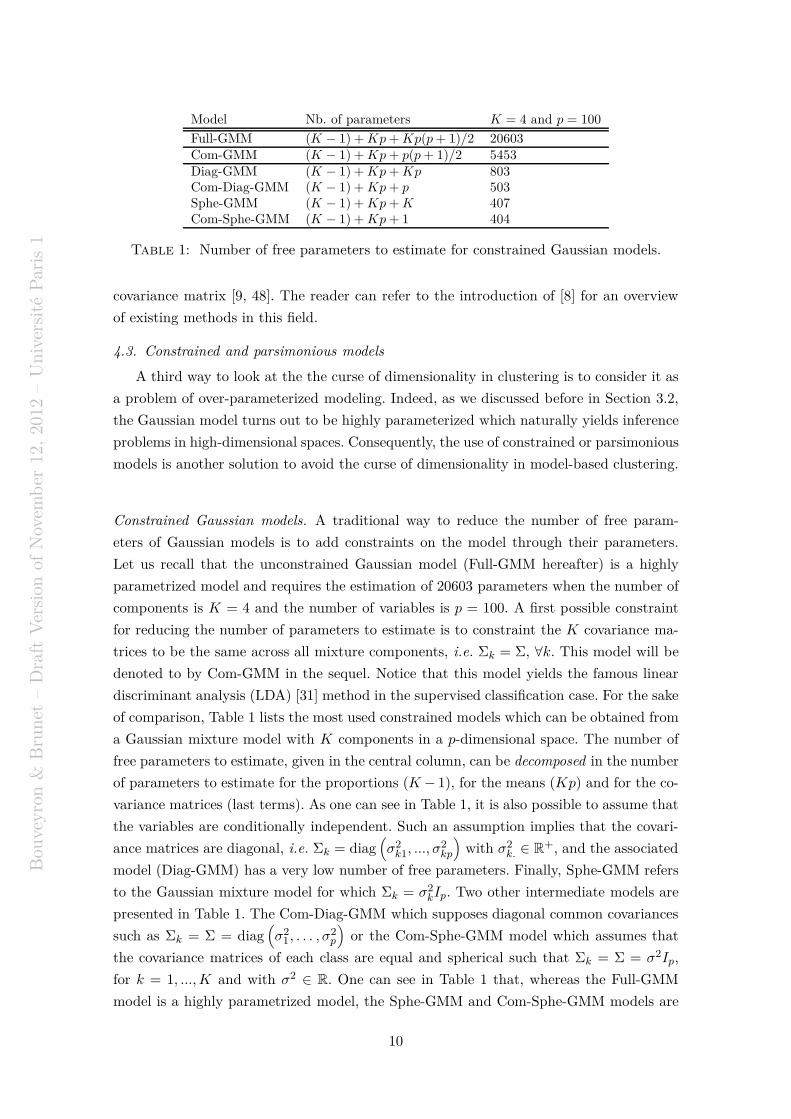
Model Nb. of parameters K = 4 and p = 100

Full-GMM (K − 1) +Kp+Kp(p+ 1)/2 20603Com-GMM (K − 1) +Kp+ p(p+ 1)/2 5453Diag-GMM (K − 1) +Kp+Kp 803Com-Diag-GMM (K − 1) +Kp+ p 503Sphe-GMM (K − 1) +Kp+K 407Com-Sphe-GMM (K − 1) +Kp+ 1 404

Table 1: Number of free parameters to estimate for constrained Gaussian models.

covariance matrix [9, 48]. The reader can refer to the introduction of [8] for an overview

of existing methods in this field.

4.3. Constrained and parsimonious models

A third way to look at the the curse of dimensionality in clustering is to consider it as

a problem of over-parameterized modeling. Indeed, as we discussed before in Section 3.2,

the Gaussian model turns out to be highly parameterized which naturally yields inference

problems in high-dimensional spaces. Consequently, the use of constrained or parsimonious

models is another solution to avoid the curse of dimensionality in model-based clustering.

Constrained Gaussian models. A traditional way to reduce the number of free param-

eters of Gaussian models is to add constraints on the model through their parameters.

Let us recall that the unconstrained Gaussian model (Full-GMM hereafter) is a highly

parametrized model and requires the estimation of 20603 parameters when the number of

components is K = 4 and the number of variables is p = 100. A first possible constraint

for reducing the number of parameters to estimate is to constraint the K covariance ma-

trices to be the same across all mixture components, i.e. Σk = Σ, ∀k. This model will be

denoted to by Com-GMM in the sequel. Notice that this model yields the famous linear

discriminant analysis (LDA) [31] method in the supervised classification case. For the sake

of comparison, Table 1 lists the most used constrained models which can be obtained from

a Gaussian mixture model with K components in a p-dimensional space. The number of

free parameters to estimate, given in the central column, can be decomposed in the number

of parameters to estimate for the proportions (K − 1), for the means (Kp) and for the co-

variance matrices (last terms). As one can see in Table 1, it is also possible to assume that

the variables are conditionally independent. Such an assumption implies that the covari-

ance matrices are diagonal, i.e. Σk = diag(

σ2k1, ..., σ

2kp

)

with σ2k. ∈ R

+, and the associated

model (Diag-GMM) has a very low number of free parameters. Finally, Sphe-GMM refers

to the Gaussian mixture model for which Σk = σ2kIp. Two other intermediate models are

presented in Table 1. The Com-Diag-GMM which supposes diagonal common covariances

such as Σk = Σ = diag(

σ21, . . . , σ

2p

)

or the Com-Sphe-GMM model which assumes that

the covariance matrices of each class are equal and spherical such that Σk = Σ = σ2Ip,

for k = 1, ...,K and with σ2 ∈ R. One can see in Table 1 that, whereas the Full-GMM

model is a highly parametrized model, the Sphe-GMM and Com-Sphe-GMM models are

10

Bou

veyro

n&

Bru

net

–D

raft

Ver

sion

ofN

ovem

ber

12,

2012

–U

niv

ersi

téP

aris

1

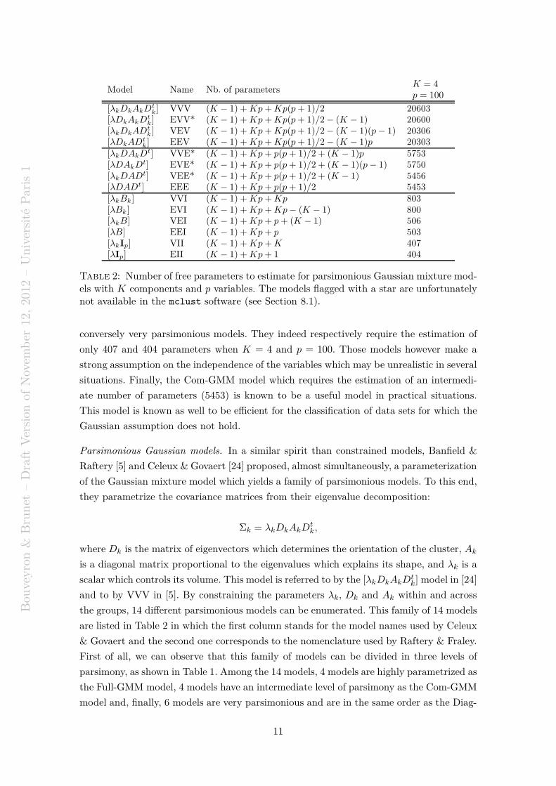
Model Name Nb. of parametersK = 4p = 100

[λkDkAkDtk] VVV (K − 1) +Kp+Kp(p+ 1)/2 20603

[λDkAkDtk] EVV* (K − 1) +Kp+Kp(p+ 1)/2 − (K − 1) 20600

[λkDkADtk] VEV (K − 1) +Kp+Kp(p+ 1)/2 − (K − 1)(p− 1) 20306

[λDkADtk] EEV (K − 1) +Kp+Kp(p+ 1)/2 − (K − 1)p 20303

[λkDAkDt] VVE* (K − 1) +Kp+ p(p+ 1)/2 + (K − 1)p 5753

[λDAkDt] EVE* (K − 1) +Kp+ p(p+ 1)/2 + (K − 1)(p− 1) 5750

[λkDADt] VEE* (K − 1) +Kp+ p(p+ 1)/2 + (K − 1) 5456

[λDADt] EEE (K − 1) +Kp+ p(p+ 1)/2 5453[λkBk] VVI (K − 1) +Kp+Kp 803[λBk] EVI (K − 1) +Kp+Kp− (K − 1) 800[λkB] VEI (K − 1) +Kp+ p+ (K − 1) 506[λB] EEI (K − 1) +Kp+ p 503[λkIp] VII (K − 1) +Kp+K 407[λIp] EII (K − 1) +Kp+ 1 404

Table 2: Number of free parameters to estimate for parsimonious Gaussian mixture mod-els with K components and p variables. The models flagged with a star are unfortunatelynot available in the mclust software (see Section 8.1).

conversely very parsimonious models. They indeed respectively require the estimation of

only 407 and 404 parameters when K = 4 and p = 100. Those models however make a

strong assumption on the independence of the variables which may be unrealistic in several

situations. Finally, the Com-GMM model which requires the estimation of an intermedi-

ate number of parameters (5453) is known to be a useful model in practical situations.

This model is known as well to be efficient for the classification of data sets for which the

Gaussian assumption does not hold.

Parsimonious Gaussian models. In a similar spirit than constrained models, Banfield &

Raftery [5] and Celeux & Govaert [24] proposed, almost simultaneously, a parameterization

of the Gaussian mixture model which yields a family of parsimonious models. To this end,

they parametrize the covariance matrices from their eigenvalue decomposition:

Σk = λkDkAkDtk,

where Dk is the matrix of eigenvectors which determines the orientation of the cluster, Ak

is a diagonal matrix proportional to the eigenvalues which explains its shape, and λk is a

scalar which controls its volume. This model is referred to by the [λkDkAkDtk] model in [24]

and to by VVV in [5]. By constraining the parameters λk, Dk and Ak within and across

the groups, 14 different parsimonious models can be enumerated. This family of 14 models

are listed in Table 2 in which the first column stands for the model names used by Celeux

& Govaert and the second one corresponds to the nomenclature used by Raftery & Fraley.

First of all, we can observe that this family of models can be divided in three levels of

parsimony, as shown in Table 1. Among the 14 models, 4 models are highly parametrized as

the Full-GMM model, 4 models have an intermediate level of parsimony as the Com-GMM

model and, finally, 6 models are very parsimonious and are in the same order as the Diag-

11

Bou

veyro

n&

Bru

net

–D

raft

Ver

sion

ofN

ovem

ber

12,

2012

–U

niv

ersi

téP

aris

1

GMM and Sphe-GMM models. Besides, this reformulation of the covariance matrices can

be viewed as a generalization of the constrained models, presented previously. For example,

the Com-GMM model is equivalent to the model [λDADt]. The model proposed by [76],

which uses the equal shape (λk = λ,∀k) and equal volume (Ak = A,∀k), turns out to

be equivalent to the model [λDkADtk]. It is worth to notice that the work of Celeux &

Govaert widens the family of parsimonious models since they add unusual models which

allow different volumes for the clusters such as the [λkDADt], [λkDAkD

t] and [λkDkADtk]

models. Furthermore, by assuming that the covariance matrix Σk are diagonal matrices,

Celeux & Govaert proposed a new parametrization Σk = λkBk where |Bk| = 1. Such a

parametrization leads to 4 additional models listed at the bottom of Table 2. Finally, by

considering the spherical shape, it leads to 2 other models: the [λkIp] and [λIp] models.

The reader can refer to [24] for more details on these models.

4.4. Discussion on classical approaches and related works

Firstly, regarding the dimension reduction solution, we would like to caution the reader

that reducing the dimension without taking into consideration the clustering goal may be

dangerous. Indeed, such a dimension reduction may yield a loss of information which could

have been useful for discriminating the groups. In particular, when PCA is used for reduc-

ing the data dimensionality, only the components associated with the largest eigenvalues

are kept. Such a practice is disproved mathematically and practically by Chang [26] who

shows that the first components do not necessary contain more discriminative information

than the others. In addition, reducing the dimension of the data may not be a good idea

since, as discussed in Section 3, it is easier to discriminate groups in high-dimensional

spaces than in lower dimensional spaces, assuming that one can build a good classifier in

high-dimensional spaces. With this point of view, subspace clustering methods are good

alternatives to dimension reduction approaches. The solution based on regularization does

not have the same drawbacks than dimension reduction and can be used with less fear.

However, all regularization techniques require the tuning of a parameter which is difficult

to tune in the unsupervised context, although this can be done easily in the supervised con-

text using cross validation. Finally, the solution which introduces parsimony in the models

is clearly a better solution in the context of model-based clustering since it proposes a

trade-off between the perfect modeling and what one can correctly estimate in practice.

We will see in the next sections that recent solutions for high-dimensional clustering are

partially based on the idea of parsimonious modeling.

5. Subspace clustering methods

Conversely to previous solutions, subspace clustering methods exploit the “empty

space” phenomenon to ease the discrimination between groups of points. To do so, they

model the data in low-dimensional subspaces and introduce some restrictions while keep-

ing all dimensions. Subspace clustering methods can be split into two categories: heuristic

and model-based methods. Heuristic methods use algorithms to search for subspaces of

12

Bou

veyro

n&

Bru

net

–D

raft

Ver

sion

ofN

ovem

ber

12,

2012

–U

niv

ersi

téP

aris

1

µ1

µ2

E1

E2

u

v

w

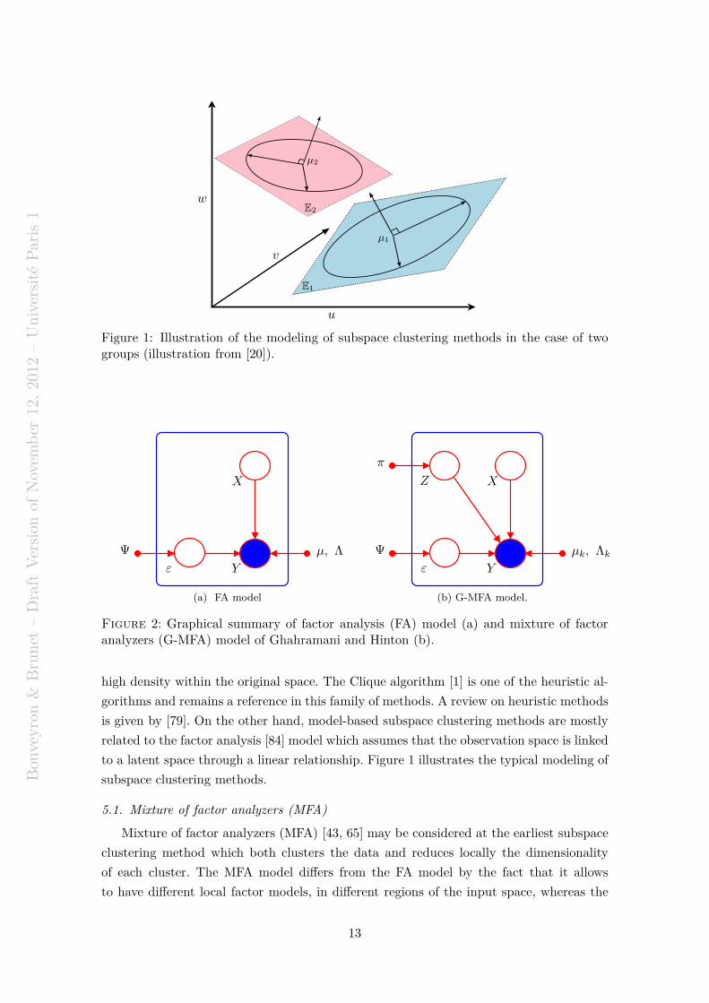
Figure 1: Illustration of the modeling of subspace clustering methods in the case of twogroups (illustration from [20]).

X

Y

µ, Λ

ε

Ψ

(a) FA model

X

Y

Z

π

µk, Λk

ε

Ψ

(b) G-MFA model.

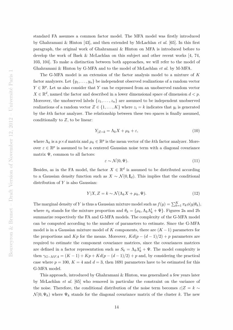
Figure 2: Graphical summary of factor analysis (FA) model (a) and mixture of factoranalyzers (G-MFA) model of Ghahramani and Hinton (b).

high density within the original space. The Clique algorithm [1] is one of the heuristic al-

gorithms and remains a reference in this family of methods. A review on heuristic methods

is given by [79]. On the other hand, model-based subspace clustering methods are mostly

related to the factor analysis [84] model which assumes that the observation space is linked

to a latent space through a linear relationship. Figure 1 illustrates the typical modeling of

subspace clustering methods.

5.1. Mixture of factor analyzers (MFA)

Mixture of factor analyzers (MFA) [43, 65] may be considered at the earliest subspace

clustering method which both clusters the data and reduces locally the dimensionality

of each cluster. The MFA model differs from the FA model by the fact that it allows

to have different local factor models, in different regions of the input space, whereas the

13

Bou

veyro

n&

Bru

net

–D

raft

Ver

sion

ofN

ovem

ber

12,

2012

–U

niv

ersi

téP

aris

1

standard FA assumes a common factor model. The MFA model was firstly introduced

by Ghahramani & Hinton [43], and then extended by McLachlan et al. [65]. In this first

paragraph, the original work of Ghahramani & Hinton on MFA is introduced before to

develop the work of Baek & McLachlan on this subject and other recent works [4, 74,

103, 104]. To make a distinction between both approaches, we will refer to the model of

Ghahramani & Hinton by G-MFA and to the model of McLachlan et al. by M-MFA.

The G-MFA model is an extension of the factor analysis model to a mixture of K

factor analyzers. Let y1, . . . , yn be independent observed realizations of a random vector

Y ∈ Rp. Let us also consider that Y can be expressed from an unobserved random vector

X ∈ Rd, named the factor and described in a lower dimensional space of dimension d < p.

Moreover, the unobserved labels z1, . . . , zn are assumed to be independent unobserved

realizations of a random vector Z ∈ 1, . . . ,K where zi = k indicates that yi is generated

by the kth factor analyzer. The relationship between these two spaces is finally assumed,

conditionally to Z, to be linear:

Y|Z=k = ΛkX + µk + ε, (10)

where Λk is a p×d matrix and µk ∈ Rp is the mean vector of the kth factor analyzer. More-

over ε ∈ Rp is assumed to be a centered Gaussian noise term with a diagonal covariance

matrix Ψ, common to all factors:

ε ∼ N (0,Ψ). (11)

Besides, as in the FA model, the factor X ∈ Rd is assumed to be distributed according

to a Gaussian density function such as X ∼ N (0, Id). This implies that the conditional

distribution of Y is also Gaussian:

Y |X,Z = k ∼ N (ΛkX + µk,Ψ). (12)

The marginal density of Y is thus a Gaussian mixture model such as f(y) =∑K

k=1 πkφ(y|θk),

where πk stands for the mixture proportion and θk = µk,ΛkΛtk + Ψ. Figures 2a and 2b

summarize respectively the FA and G-MFA models. The complexity of the G-MFA model

can be computed according to the number of parameters to estimate. Since the G-MFA

model is in a Gaussian mixture model of K components, there are (K − 1) parameters for

the proportions and Kp for the means. Moreover, Kd(p − (d − 1)/2) + p parameters are

required to estimate the component covariance matrices, since the covariances matrices

are defined in a factor representation such as Sk = ΛkΛtk + Ψ. The model complexity is

then γG−MF A = (K − 1) +Kp+Kd(p− (d− 1)/2) + p and, by considering the practical

case where p = 100, K = 4 and d = 3, then 1691 parameters have to be estimated for this

G-MFA model.

This approach, introduced by Ghahramani & Hinton, was generalized a few years later

by McLachlan et al. [65] who removed in particular the constraint on the variance of

the noise. Therefore, the conditional distribution of the noise term becomes ε|Z = k ∼

N (0,Ψk) where Ψk stands for the diagonal covariance matrix of the cluster k. The new

14

Bou

veyro

n&

Bru

net

–D

raft

Ver

sion

ofN

ovem

ber

12,

2012

–U

niv

ersi

téP

aris

1

Model name Cov. structure Nb. of parametersK = 4,d = 3p = 100

M-MFA Sk = ΛkΛtk + Ψk (K − 1) +Kp+Kd[p− (d− 1)/2] +Kp 1991

G-MFA Sk = ΛkΛtk + Ψ (K − 1) +Kp+Kd[p− (d− 1)/2] + p 1691

MCFA Sk = AΩkAt + Ψ (K − 1) +Kd+ p+ d[p− (d+ 1)/2] +Kd(d+ 1)/2 433

HFMA Sk = V ΩkVt + Ψ (K − 1) + (K − 1)d+ p+ d[p− (d− 1)/2] + (K − 1)d(d+ 1)/2 427

MCUFSA Sk = A∆kAt + λIp (K − 1) +Kd+ 1 + d[p− (d+ 1)/2] +Kd 322

A is defined such as AtA = Id, V such as VΨ−1V t is diagonal with decreasing order and ∆k is a diagonal matrix.

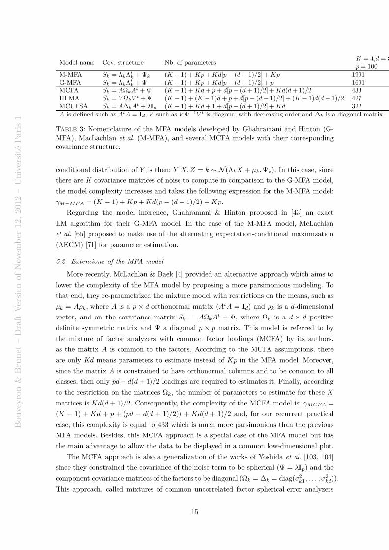
Table 3: Nomenclature of the MFA models developed by Ghahramani and Hinton (G-MFA), MacLachlan et al. (M-MFA), and several MCFA models with their correspondingcovariance structure.

conditional distribution of Y is then: Y |X,Z = k ∼ N (ΛkX + µk,Ψk). In this case, since

there are K covariance matrices of noise to compute in comparison to the G-MFA model,

the model complexity increases and takes the following expression for the M-MFA model:

γM−MF A = (K − 1) +Kp+Kd(p− (d− 1)/2) +Kp.

Regarding the model inference, Ghahramani & Hinton proposed in [43] an exact

EM algorithm for their G-MFA model. In the case of the M-MFA model, McLachlan

et al. [65] proposed to make use of the alternating expectation-conditional maximization

(AECM) [71] for parameter estimation.

5.2. Extensions of the MFA model

More recently, McLachlan & Baek [4] provided an alternative approach which aims to

lower the complexity of the MFA model by proposing a more parsimonious modeling. To

that end, they re-parametrized the mixture model with restrictions on the means, such as

µk = Aρk, where A is a p × d orthonormal matrix (AtA = Id) and ρk is a d-dimensional

vector, and on the covariance matrix Sk = AΩkAt + Ψ, where Ωk is a d × d positive

definite symmetric matrix and Ψ a diagonal p × p matrix. This model is referred to by

the mixture of factor analyzers with common factor loadings (MCFA) by its authors,

as the matrix A is common to the factors. According to the MCFA assumptions, there

are only Kd means parameters to estimate instead of Kp in the MFA model. Moreover,

since the matrix A is constrained to have orthonormal columns and to be common to all

classes, then only pd− d(d+ 1)/2 loadings are required to estimates it. Finally, according

to the restriction on the matrices Ωk, the number of parameters to estimate for these K

matrices is Kd(d+ 1)/2. Consequently, the complexity of the MCFA model is: γMCF A =

(K − 1) + Kd + p + (pd − d(d + 1)/2)) + Kd(d + 1)/2 and, for our recurrent practical

case, this complexity is equal to 433 which is much more parsimonious than the previous

MFA models. Besides, this MCFA approach is a special case of the MFA model but has

the main advantage to allow the data to be displayed in a common low-dimensional plot.

The MCFA approach is also a generalization of the works of Yoshida et al. [103, 104]

since they constrained the covariance of the noise term to be spherical (Ψ = λIp) and the

component-covariance matrices of the factors to be diagonal (Ωk = ∆k = diag(σ2k1, . . . , σ

2kd)).

This approach, called mixtures of common uncorrelated factor spherical-error analyzers

15

Bou

veyro

n&

Bru

net

–D

raft

Ver

sion

ofN

ovem

ber

12,

2012

–U

niv

ersi

téP

aris

1

Model name Cov. structure Nb. of parametersK = 4,d = 3p = 100

UUUU - UUU Sk = ΛkΛtk + Ψk (K − 1) +Kp+Kd[p− (d− 1)/2] +Kp 1991

UUCU - Sk = ΛkΛtk + ωk∆k (K − 1) +Kp+Kd[p− (d− 1)/2] + [1 +K(p− 1)] 1988

UCUU - Sk = ΛkΛtk + ωk∆ (K − 1) +Kp+Kd[p− (d− 1)/2] + [K + (p− 1)] 1694

UCCU - UCU Sk = ΛkΛtk + Ψ (K − 1) +Kp+Kd[p− (d− 1)/2] + p 1691

UCUC - UUC Sk = ΛkΛtk + ψkIp (K − 1) +Kp+Kd[p− (d− 1)/2] +K 1595

UCCC - UCC Sk = ΛkΛtk + ψIp (K − 1) +Kp+Kd[p− (d− 1)/2] + 1 1592

CUUU - CUU Sk = ΛΛt + Ψk (K − 1) +Kp+ d[p− (d− 1)/2] +Kp 1100CUCU - Sk = ΛΛt + ω∆k (K − 1) +Kp+ d[p− (d− 1)/2] + [1 +K(p− 1)] 1097CCUU - Sk = ΛΛt + ωk∆ (K − 1) +Kp+ d[p− (d− 1)/2] + [K + (p− 1)] 803CCCU - CCU Sk = ΛΛt + Ψ (K − 1) +Kp+ d[p− (d− 1)/2] + p 800CCUC - CUC Sk = ΛΛt + ψkIp (K − 1) +Kp+ d[p− (d− 1)/2] +K 704CCCC - CCC Sk = ΛΛt + ψIp (K − 1) +Kp+ d[p− (d− 1)/2] + 1 701where ωk ∈ R

+and |∆k| = 1.

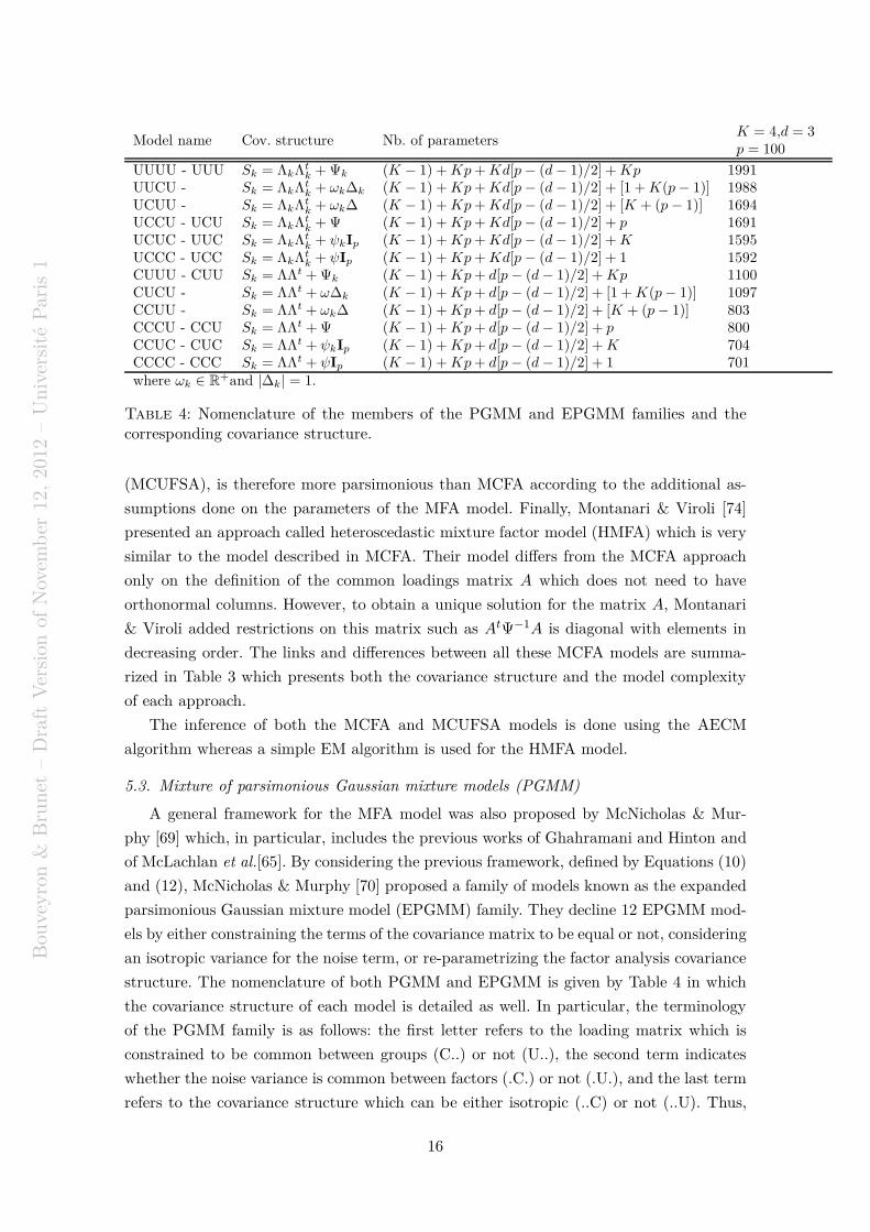
Table 4: Nomenclature of the members of the PGMM and EPGMM families and thecorresponding covariance structure.

(MCUFSA), is therefore more parsimonious than MCFA according to the additional as-

sumptions done on the parameters of the MFA model. Finally, Montanari & Viroli [74]

presented an approach called heteroscedastic mixture factor model (HMFA) which is very

similar to the model described in MCFA. Their model differs from the MCFA approach

only on the definition of the common loadings matrix A which does not need to have

orthonormal columns. However, to obtain a unique solution for the matrix A, Montanari

& Viroli added restrictions on this matrix such as AtΨ−1A is diagonal with elements in

decreasing order. The links and differences between all these MCFA models are summa-

rized in Table 3 which presents both the covariance structure and the model complexity

of each approach.

The inference of both the MCFA and MCUFSA models is done using the AECM

algorithm whereas a simple EM algorithm is used for the HMFA model.

5.3. Mixture of parsimonious Gaussian mixture models (PGMM)

A general framework for the MFA model was also proposed by McNicholas & Mur-

phy [69] which, in particular, includes the previous works of Ghahramani and Hinton and

of McLachlan et al.[65]. By considering the previous framework, defined by Equations (10)

and (12), McNicholas & Murphy [70] proposed a family of models known as the expanded

parsimonious Gaussian mixture model (EPGMM) family. They decline 12 EPGMM mod-

els by either constraining the terms of the covariance matrix to be equal or not, considering

an isotropic variance for the noise term, or re-parametrizing the factor analysis covariance

structure. The nomenclature of both PGMM and EPGMM is given by Table 4 in which

the covariance structure of each model is detailed as well. In particular, the terminology

of the PGMM family is as follows: the first letter refers to the loading matrix which is

constrained to be common between groups (C..) or not (U..), the second term indicates

whether the noise variance is common between factors (.C.) or not (.U.), and the last term

refers to the covariance structure which can be either isotropic (..C) or not (..U). Thus,

16

Bou

veyro

n&

Bru

net

–D

raft

Ver

sion

ofN

ovem

ber

12,

2012

–U

niv

ersi

téP

aris

1

X

Y

Z

πk µk, dk

ak1, ..., akdk

Qk

ε

bk

(a) HD-GMM model

X

Y

Z

πk µk

Σk

U

ε

Ψ

(b) DLM model

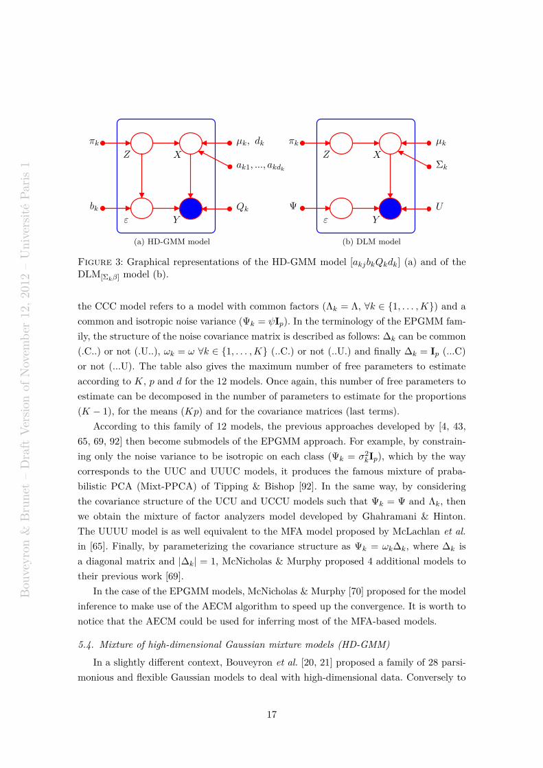
Figure 3: Graphical representations of the HD-GMM model [akjbkQkdk] (a) and of theDLM[Σkβ] model (b).

the CCC model refers to a model with common factors (Λk = Λ, ∀k ∈ 1, . . . ,K) and a

common and isotropic noise variance (Ψk = ψIp). In the terminology of the EPGMM fam-

ily, the structure of the noise covariance matrix is described as follows: ∆k can be common

(.C..) or not (.U..), ωk = ω ∀k ∈ 1, . . . ,K (..C.) or not (..U.) and finally ∆k = Ip (...C)

or not (...U). The table also gives the maximum number of free parameters to estimate

according to K, p and d for the 12 models. Once again, this number of free parameters to

estimate can be decomposed in the number of parameters to estimate for the proportions

(K − 1), for the means (Kp) and for the covariance matrices (last terms).

According to this family of 12 models, the previous approaches developed by [4, 43,

65, 69, 92] then become submodels of the EPGMM approach. For example, by constrain-

ing only the noise variance to be isotropic on each class (Ψk = σ2kIp), which by the way

corresponds to the UUC and UUUC models, it produces the famous mixture of praba-

bilistic PCA (Mixt-PPCA) of Tipping & Bishop [92]. In the same way, by considering

the covariance structure of the UCU and UCCU models such that Ψk = Ψ and Λk, then

we obtain the mixture of factor analyzers model developed by Ghahramani & Hinton.

The UUUU model is as well equivalent to the MFA model proposed by McLachlan et al.

in [65]. Finally, by parameterizing the covariance structure as Ψk = ωk∆k, where ∆k is

a diagonal matrix and |∆k| = 1, McNicholas & Murphy proposed 4 additional models to

their previous work [69].

In the case of the EPGMM models, McNicholas & Murphy [70] proposed for the model

inference to make use of the AECM algorithm to speed up the convergence. It is worth to

notice that the AECM could be used for inferring most of the MFA-based models.

5.4. Mixture of high-dimensional Gaussian mixture models (HD-GMM)

In a slightly different context, Bouveyron et al. [20, 21] proposed a family of 28 parsi-

monious and flexible Gaussian models to deal with high-dimensional data. Conversely to

17

Bou

veyro

n&

Bru

net

–D

raft

Ver

sion

ofN

ovem

ber

12,

2012

–U

niv

ersi

téP

aris

1

the previous approaches, this family of GMM was directly proposed in both supervised

and unsupervised classification contexts. In order to ease the designation of this family,

we propose to refer to these Gaussian models for high-dimensional data by the acronym

HD-GMM. Bouveyron et al. [20] proposed to constraint the GMM model through the

eigen-decomposition of the covariance matrix Σk of the kth group:

Σk = QkΛkQtk,

where Qk is a p × p orthogonal matrix which contains the eigenvectors of Σk and Λk is a

p × p diagonal matrix containing the associated eigenvalues (sorted in decreasing order).

The key idea of the work of Bouveyron et al. is to reparametrize the matrix Λk, such as

Σk has only dk + 1 different eigenvalues:

Λk = diag (ak1, . . . , akdk, bk, . . . , bk) ,

where the dk first values ak1, . . . , akdkparametrize the variance in the group-specific sub-

space and the p − dk last terms, the bk’s model the variance of the noise and dk < p.

With this parametrization, these parsimonious models assume that, conditionally to the

groups, the noise variance of each cluster k is isotropic and is contained in a subspace

which is orthogonal to the subspace of the kth group. Following the classical parsimony

strategy, the authors proposed a family of parsimonious models from a very general model,

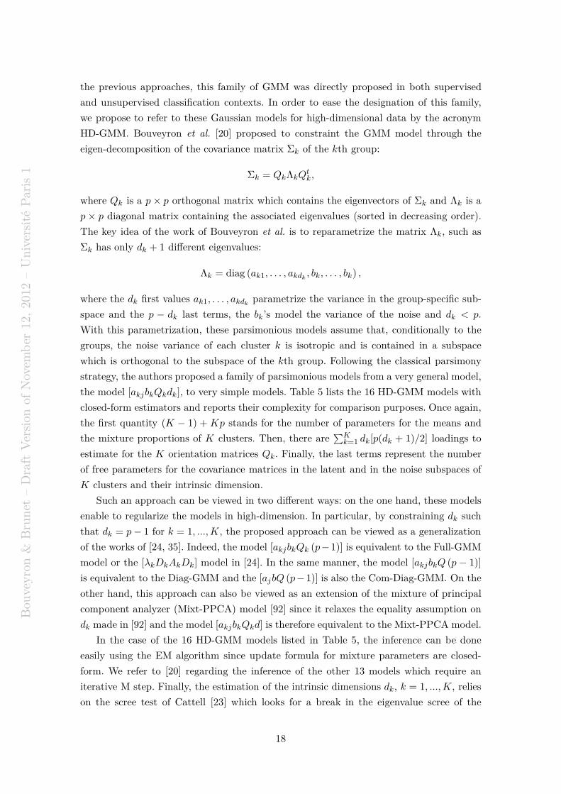
the model [akjbkQkdk], to very simple models. Table 5 lists the 16 HD-GMM models with

closed-form estimators and reports their complexity for comparison purposes. Once again,

the first quantity (K − 1) + Kp stands for the number of parameters for the means and

the mixture proportions of K clusters. Then, there are∑K

k=1 dk[p(dk + 1)/2] loadings to

estimate for the K orientation matrices Qk. Finally, the last terms represent the number

of free parameters for the covariance matrices in the latent and in the noise subspaces of

K clusters and their intrinsic dimension.

Such an approach can be viewed in two different ways: on the one hand, these models

enable to regularize the models in high-dimension. In particular, by constraining dk such

that dk = p− 1 for k = 1, ...,K, the proposed approach can be viewed as a generalization

of the works of [24, 35]. Indeed, the model [akjbkQk (p−1)] is equivalent to the Full-GMM

model or the [λkDkAkDk] model in [24]. In the same manner, the model [akjbkQ (p − 1)]

is equivalent to the Diag-GMM and the [ajbQ (p− 1)] is also the Com-Diag-GMM. On the

other hand, this approach can also be viewed as an extension of the mixture of principal

component analyzer (Mixt-PPCA) model [92] since it relaxes the equality assumption on

dk made in [92] and the model [akjbkQkd] is therefore equivalent to the Mixt-PPCA model.

In the case of the 16 HD-GMM models listed in Table 5, the inference can be done

easily using the EM algorithm since update formula for mixture parameters are closed-

form. We refer to [20] regarding the inference of the other 13 models which require an

iterative M step. Finally, the estimation of the intrinsic dimensions dk, k = 1, ...,K, relies

on the scree test of Cattell [23] which looks for a break in the eigenvalue scree of the

18

Bou

veyro

n&

Bru

net

–D

raft

Ver

sion

ofN

ovem

ber

12,

2012

–U

niv

ersi

téP

aris

1

Model name Nb. of parametersp = 100K = 4, d = 3

[akjbkQkdk] (K − 1) +Kp+∑K

k=1 dk[p− (dk + 1)/2] +∑K

k=1 dk + 2K 1599

[akjbQkdk] (K − 1) +Kp+∑K

k=1 dk[p− (dk + 1)/2] +∑K

k=1 dk + 1 +K 1596

[akbkQkdk] (K − 1) +Kp+∑K

k=1 dk[p− (dk + 1)/2] + 3K 1591

[abkQkdk] (K − 1) +Kp+∑K

k=1 dk[p− (dk + 1)/2] + 1 + 2K 1588

[akbQkdk] (K − 1) +Kp+∑K

k=1 dk[p− (dk + 1)/2] + 1 + 2K 1588

[abQkdk] (K − 1) +Kp+∑K

k=1 dk[p− (dk + 1)/2] + 2 +K 1585[akjbkQkd] (K − 1) +Kp+Kd[p− (d+ 1)/2] +Kd+K + 1 1596[ajbkQkd] (K − 1) +Kp+Kd[p− (d+ 1)/2] + d+K + 1 1587[akjbQkd] (K − 1) +Kp+Kd[p− (d+ 1)/2] +Kd+ 2 1593[ajbQkd] (K − 1) +Kp+Kd[p− (d+ 1)/2] + d+ 2 1584[akbkQkd] (K − 1) +Kp+Kd[p− (d+ 1)/2] + 2K + 1 1588[abkQkd] (K − 1) +Kp+Kd[p− (d+ 1)/2] +K + 2 1585[akbQkd] (K − 1) +Kp+Kd[p− (d+ 1)/2] +K + 2 1585[abQkd] (K − 1) +Kp+Kd[p− (d+ 1)/2] + 3 1582[ajbQd] (K − 1) +Kp+ d[p− (d+ 1)/2] + d+ 2 702[abQd] (K − 1) +Kp+ d[p− (d+ 1)/2] + 3 700

Table 5: Nomenclature for the members of the Hd-GMM family and the number ofparameters to estimate. For the numerical example, the intrinsic dimension of the clustershas been fixed to dk = d = 3, ∀k = 1, . . . ,K.

empirical covariance matrix of each group. Let us finally notice that Bouveyron et al. [19]

have demonstrated the surprising result that the maximum likelihood estimator of the

intrinsic dimensions dk is asymptotically consistent in the case of the model [akbkQkdk].

5.5. The discriminative latent mixture (DLM) models

Recently, Bouveyron & Brunet [17] proposed a family of mixture models which fit the

data into a common and discriminative subspace. This mixture model, called the discrim-

inative latent mixture (DLM) model, differs from the FA-based models in the fact that

the latent subspace is common to all groups and is assumed to be the most discriminative

subspace of dimension d. This latter feature of the DLM model makes it significantly dif-

ferent from the other FA-based models. Indeed, roughly speaking, the FA-based models

choose the latent subspace(s) maximizing the projected variance whereas the DLM model

chooses the latent subspace which maximizes the separation between the groups.

Let us nevertheless start with a FA-like modeling. Let Y ∈ Rp be the observed random

vector and let Z ∈ 1, . . . ,K be once again the unobserved random variable to predict.

The DLM model then assumes that Y is linked to a latent random vector X ∈ E through

a linear relationship of the form Y = UX + ε, where E ⊂ Rp is assumed to be the

most discriminative subspace of dimension d ≤ K − 1 such that 0 ∈ E, K < p, U is

a p × d orthonormal matrix common to the K groups and satisfying U tU = Id, and

ε ∼ N (0,Ψ) models the non discriminative information. Besides, within the latent space

and conditionally to Z = k, X is assumed to be distributed as X|Z = k ∼ N (µk,Σk)

where µk ∈ Rd and Σk ∈ R

d×d are respectively the mean vector and the covariance matrix

19

Bou

veyro

n&

Bru

net

–D

raft

Ver

sion

ofN

ovem

ber

12,

2012

–U

niv

ersi

téP

aris

1

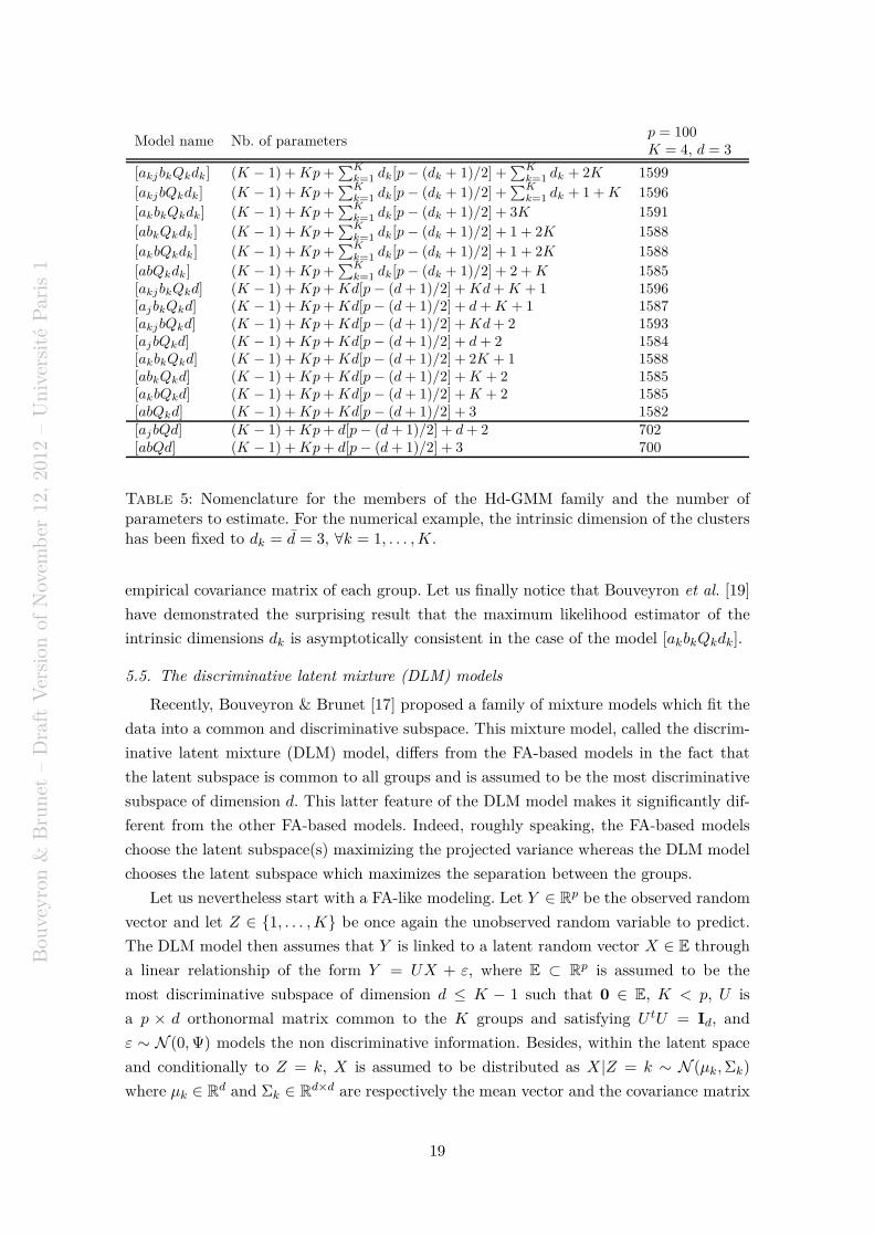
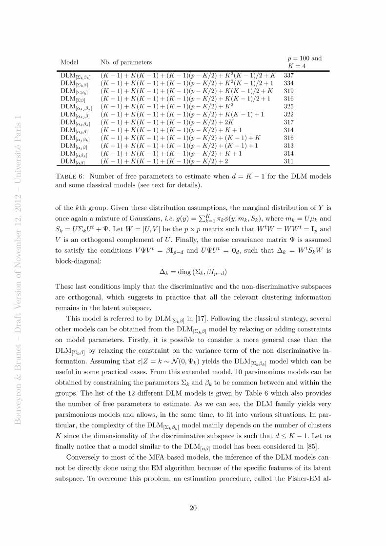
Model Nb. of parametersp = 100 andK = 4

DLM[Σkβk] (K − 1) +K(K − 1) + (K − 1)(p−K/2) +K2(K − 1)/2 +K 337DLM[Σkβ] (K − 1) +K(K − 1) + (K − 1)(p−K/2) +K2(K − 1)/2 + 1 334DLM[Σβk] (K − 1) +K(K − 1) + (K − 1)(p−K/2) +K(K − 1)/2 +K 319DLM[Σβ] (K − 1) +K(K − 1) + (K − 1)(p−K/2) +K(K − 1)/2 + 1 316DLM[αkjβk] (K − 1) +K(K − 1) + (K − 1)(p−K/2) +K2 325DLM[αkjβ] (K − 1) +K(K − 1) + (K − 1)(p−K/2) +K(K − 1) + 1 322DLM[αkβk] (K − 1) +K(K − 1) + (K − 1)(p−K/2) + 2K 317DLM[αkβ] (K − 1) +K(K − 1) + (K − 1)(p−K/2) +K + 1 314DLM[αjβk] (K − 1) +K(K − 1) + (K − 1)(p−K/2) + (K − 1) +K 316DLM[αjβ] (K − 1) +K(K − 1) + (K − 1)(p−K/2) + (K − 1) + 1 313DLM[αβk] (K − 1) +K(K − 1) + (K − 1)(p−K/2) +K + 1 314DLM[αβ] (K − 1) +K(K − 1) + (K − 1)(p−K/2) + 2 311

Table 6: Number of free parameters to estimate when d = K − 1 for the DLM modelsand some classical models (see text for details).

of the kth group. Given these distribution assumptions, the marginal distribution of Y is

once again a mixture of Gaussians, i.e. g(y) =∑K

k=1 πkφ(y;mk, Sk), where mk = Uµk and

Sk = UΣkUt + Ψ. Let W = [U, V ] be the p× p matrix such that W tW = WW t = Ip and

V is an orthogonal complement of U . Finally, the noise covariance matrix Ψ is assumed

to satisfy the conditions VΨV t = βIp−d and UΨU t = 0d, such that ∆k = W tSkW is

block-diagonal:

∆k = diag (Σk, βIp−d)

These last conditions imply that the discriminative and the non-discriminative subspaces

are orthogonal, which suggests in practice that all the relevant clustering information

remains in the latent subspace.

This model is referred to by DLM[Σkβ] in [17]. Following the classical strategy, several

other models can be obtained from the DLM[Σkβ] model by relaxing or adding constraints

on model parameters. Firstly, it is possible to consider a more general case than the

DLM[Σkβ] by relaxing the constraint on the variance term of the non discriminative in-

formation. Assuming that ε|Z = k ∼ N (0,Ψk) yields the DLM[Σkβk] model which can be

useful in some practical cases. From this extended model, 10 parsimonious models can be

obtained by constraining the parameters Σk and βk to be common between and within the

groups. The list of the 12 different DLM models is given by Table 6 which also provides

the number of free parameters to estimate. As we can see, the DLM family yields very

parsimonious models and allows, in the same time, to fit into various situations. In par-

ticular, the complexity of the DLM[Σkβk] model mainly depends on the number of clusters

K since the dimensionality of the discriminative subspace is such that d ≤ K − 1. Let us

finally notice that a model similar to the DLM[αβ] model has been considered in [85].

Conversely to most of the MFA-based models, the inference of the DLM models can-

not be directly done using the EM algorithm because of the specific features of its latent

subspace. To overcome this problem, an estimation procedure, called the Fisher-EM al-

20

Bou

veyro

n&

Bru

net

–D

raft

Ver

sion

ofN

ovem

ber

12,

2012

–U

niv

ersi

téP

aris

1

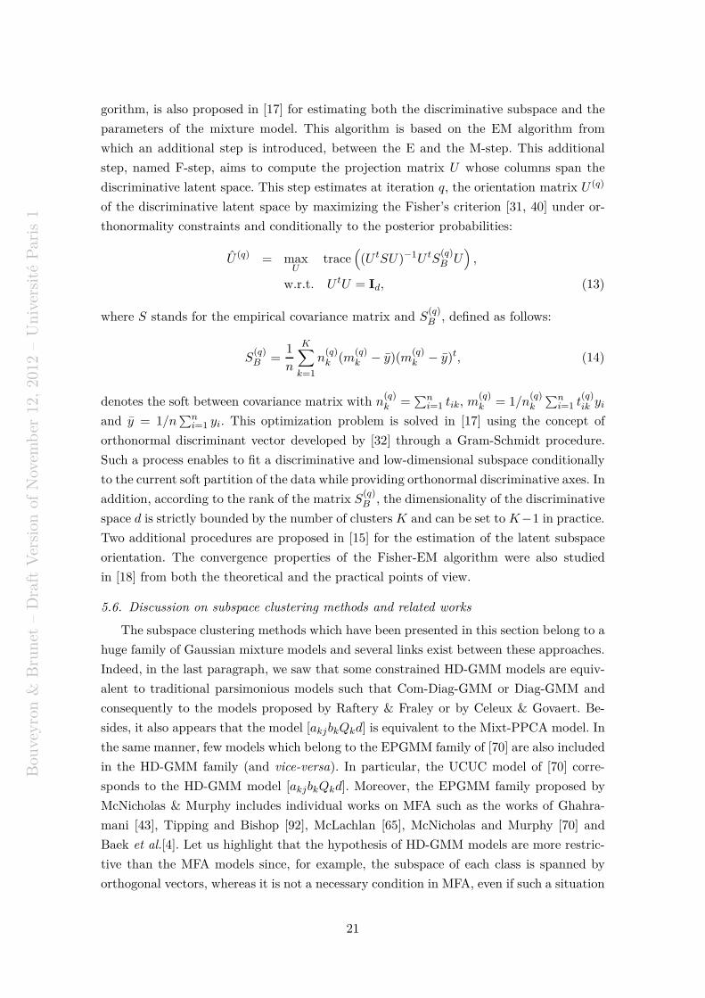
gorithm, is also proposed in [17] for estimating both the discriminative subspace and the

parameters of the mixture model. This algorithm is based on the EM algorithm from

which an additional step is introduced, between the E and the M-step. This additional

step, named F-step, aims to compute the projection matrix U whose columns span the

discriminative latent space. This step estimates at iteration q, the orientation matrix U (q)

of the discriminative latent space by maximizing the Fisher’s criterion [31, 40] under or-

thonormality constraints and conditionally to the posterior probabilities:

U (q) = maxU

trace(

(U tSU)−1U tS(q)B U

)

,

w.r.t. U tU = Id, (13)

where S stands for the empirical covariance matrix and S(q)B , defined as follows:

S(q)B =

1

n

K∑

k=1

n(q)k (m

(q)k − y)(m

(q)k − y)t, (14)

denotes the soft between covariance matrix with n(q)k =

∑ni=1 tik, m

(q)k = 1/n

(q)k

∑ni=1 t

(q)ik yi

and y = 1/n∑n

i=1 yi. This optimization problem is solved in [17] using the concept of

orthonormal discriminant vector developed by [32] through a Gram-Schmidt procedure.

Such a process enables to fit a discriminative and low-dimensional subspace conditionally

to the current soft partition of the data while providing orthonormal discriminative axes. In

addition, according to the rank of the matrix S(q)B , the dimensionality of the discriminative

space d is strictly bounded by the number of clusters K and can be set to K−1 in practice.

Two additional procedures are proposed in [15] for the estimation of the latent subspace

orientation. The convergence properties of the Fisher-EM algorithm were also studied

in [18] from both the theoretical and the practical points of view.

5.6. Discussion on subspace clustering methods and related works

The subspace clustering methods which have been presented in this section belong to a

huge family of Gaussian mixture models and several links exist between these approaches.

Indeed, in the last paragraph, we saw that some constrained HD-GMM models are equiv-

alent to traditional parsimonious models such that Com-Diag-GMM or Diag-GMM and

consequently to the models proposed by Raftery & Fraley or by Celeux & Govaert. Be-

sides, it also appears that the model [akjbkQkd] is equivalent to the Mixt-PPCA model. In

the same manner, few models which belong to the EPGMM family of [70] are also included

in the HD-GMM family (and vice-versa). In particular, the UCUC model of [70] corre-

sponds to the HD-GMM model [akjbkQkd]. Moreover, the EPGMM family proposed by

McNicholas & Murphy includes individual works on MFA such as the works of Ghahra-

mani [43], Tipping and Bishop [92], McLachlan [65], McNicholas and Murphy [70] and

Baek et al.[4]. Let us highlight that the hypothesis of HD-GMM models are more restric-

tive than the MFA models since, for example, the subspace of each class is spanned by

orthogonal vectors, whereas it is not a necessary condition in MFA, even if such a situation

21

Bou

veyro

n&

Bru

net

–D

raft

Ver

sion

ofN

ovem

ber

12,

2012

–U

niv

ersi

téP

aris

1

EPGMM PGMM MFA models Hd-GMMTraditional

GMMParsimonious

clustering modelMclust

McNicholas and Murphy

McLachlan and Peel,

Ghahramani and Hinton,

Bishop and Tipping

Bouveyron, Girard

and Schmid

Scott and Symons,

Marriott, etc.

Celeux and

Govaert

Banfield, Fraley

and Raftery

[akjbkQkdk]

[akjbQkdk]

[akbkQkdk]

[abkQkdk]

CCUU [abQkdk]

UCUU [ajbkQkd]

CUCU [akjbQkd]

UUCU [ajbQkd] [λkBk]

CUUU CUU [akbkQkd] [λBk]

CCUC CUC [abkQkd] [λkB]

UUCC UUC [akbQkd] [λB]

CCCC CCC [abQkd] [λDkADtk] EEV

CCCU CCU M-MFA [ajbQd] [λkDkADtk] VEV

UUUU UUU G-MFA [abQd] [λkAk] VVI

UUUC UUC Mixt-PPCA [akjbkQkd] [λAk] EVI

[akjbkIp (p− 1)] Diag-GMM [λkA] VEI

[akjbkQk (p− 1)] Full-GMM [λkDkAkDtk] VVV

[ajbQ (p− 1)] Com-GMM [λDADt] EEE

Sphe-GMM [λkIp] VII

Com-Sphe-GMM [λIp] EII

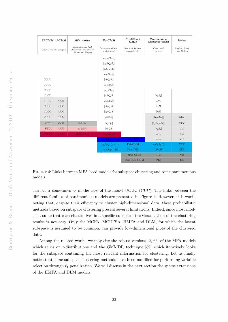
Figure 4: Links between MFA-bsed models for subspace clustering and some parsimoniousmodels.

can occur sometimes as in the case of the model UCUC (CUC). The links between the

different families of parsimonious models are presented in Figure 4. However, it is worth

noting that, despite their efficiency to cluster high-dimensional data, these probabilistic

methods based on subspace clustering present several limitations. Indeed, since most mod-

els assume that each cluster lives in a specific subspace, the visualization of the clustering

results is not easy. Only the MCFA, MCUFSA, HMFA and DLM, for which the latent

subspace is assumed to be common, can provide low-dimensional plots of the clustered

data.

Among the related works, we may cite the robust versions [2, 66] of the MFA models

which relies on t-distributions and the GMMDR technique [89] which iteratively looks

for the subspace containing the most relevant information for clustering. Let us finally

notice that some subspace clustering methods have been modified for performing variable

selection through ℓ1 penalization. We will discuss in the next section the sparse extensions

of the HMFA and DLM models.

22

Bou

veyro

n&

Bru

net

–D

raft

Ver

sion

ofN

ovem

ber

12,

2012

–U

niv

ersi

téP

aris

1

6. Variable selection for clustering

Conversely to the approaches of the previous section, several recent works have been

interested to simultaneously cluster data and reduce their dimensionality by selecting

relevant variables for the clustering task. A common assumption to these works is that

the true underlying clusters are assumed to differ only with respect to some of the original

features. The clustering task aims therefore to group the data on a subset of relevant

features. This presents two practical advantages: clustering results should be improved by

removing non informative features and the interpretation of the obtained clusters should

be eased by the meaning of retained variables. In the literature, variable selection for

clustering is handled in two different ways.

On the one hand, some authors such as [49, 54, 57, 83] tackle the problem of variable

selection for model-based clustering within a Bayesian framework. In particular, the de-

termination of the role of each variable is recast as a model selection problem. On the

other hand, penalized clustering criteria have also been proposed to deal with the problem

of variable selection in clustering. In the Gaussian mixture model context, several works,

such as [78, 96, 101, 105] in particular, introduced a penalty term in the log-likelihood

function in order to yield sparsity in the features.

6.1. Variable selection as a model selection problem

The underlying idea of the works of Law et al. [49], Raftery and Dean [83] and Maugis et

al. [57] is to find the variables which are relevant for the clustering task. The determination

of the role of each variable is in particular apprehended in [57, 83] as a model selection

problem in the GMM context. In particular, Raftery & Dean and Maugis et al. consider a

collection of parsimonious and interpretable models, developed by Banfield & Raftery [5]

and Celeux & Govaert [24], based on a specific decomposition of the mixture component

variance matrix (see Section 4 for more details).

In the Raftery & Dean’s approach, the authors define two different sets of variables:

S which denotes the set of relevant variables and Sc which is the set containing the

irrelevant variables. An interesting aspect of their approach is that they do not assume

that the irrelevant variables are independent of the clustering variables conversely to Law

et al. [49]. In particular, they define the irrelevant variables as those which are independent

of the clustering but which remain dependent of the set of relevant variables according to

a linear relationship. The models in competition are compared with the integrated log-

likelihood via a BIC approximation. Thus, the selected model maximizes the following

quantity:

(

K, m, S)

= arg max(K,m,r,ℓ,V )

BICclust(yS |K,m) + BICreg(ySc |yS)

, (15)

where K is the number of clusters and m ∈ M is a model which belongs to the family of

parsimonious models available in the mclust [34] software. Note that the quantity to be

maximized in expression (15), can be decomposed into two parts: the first term corresponds

23

Bou

veyro

n&

Bru

net

–D

raft

Ver

sion

ofN

ovem

ber

12,

2012

–U

niv

ersi

téP

aris

1

to the Gaussian mixture model of K components on the subset of relevant variables S,

whereas the second one is relative to the regression of irrelevant variables in Sc on the

set of all clustering variables in S. However, the dependence assumption which defines the

irrelevant set of variables according to all the relevant ones remains debatable. Indeed, on

the one hand, considering only the case where the irrelevant variables are independent on

both the clustering and the relevant partition, as it was considered in the work of Law

et al. [49], seems to be unrealistic. On the other hand, considering that all the irrelevant

variables depends on the relevant variables by a linear relationship seems to be as well a

strong hypothesis which may be not valid in certain practical cases. An other limitation

of the Raftery & Dean’s procedure is linked to their variable selection algorithm. Indeed,

they proposed in [83] a forward-stepwise algorithm which considers only few variables at

the beginning and which prevents from taking into account the block interactions between

variables.

To overcome these limitations, Maugis et al. [25, 57, 58] relax such restrictions and

propose a more general variable role modeling. They define two subsets of variables: on

the one hand, the relevant ones, which are grouped in S and, on the other hand, its

complementary Sc, which is formed by the irrelevant variables. Maugis et al. consider two

types of behaviors among these irrelevant variables: a subset U of irrelevant variables which

can be explained by a linear regression from a subset R of the clustering variables and

a subset W of irrelevant variables which are totally independent of all relevant variables.

Such a variable partition allows to both consider the approaches developed by Law et

al. [49] and by Raftery & Dean [83]. It is referred to by the model collection SRUW. From

this characterization, the authors also recast the variable selection problem into a model

selection problem through an approximation of the integrated log-likelihood. Then the

selected model satisfies:

(

K, m, r, h, V)

= arg max(K,m,r,h,V )

BICclust(yS |K,m) + BICreg(yU |r,yR) + BICind(yW |h)

,

(16)

where V = (S,R,U ,W) stands for the variable partition. The first term of this expression,

called BICclust, corresponds to the BIC criterion [86] for a Gaussian mixture of K compo-

nents on the relevant subset of variables S. The model m belongs here to a collection of

28 parsimonious models which are available in the Mixmod software [11] and include the

GMM family introduced by Celeux & Govaert [24]. The second term denoted by BICreg, is

linked to the BIC criterion for a linear regression of the irrelevant variables U on a subset

of clustering variables R. Note that the index r stands for the structure of the covariance

matrix which can be assumed to be spherical, diagonal or non-constraint. Finally, the last

term depicts the BIC criterion for a Gaussian density on the variable subset W indepen-

dent of the clustering variables. This Gaussian marginal distribution is characterized by a

variance matrix σ which is constrained to be either diagonal or spherical and is specified

by the index h in the expression (16).

24

Bou

veyro

n&

Bru

net

–D

raft

Ver

sion

ofN

ovem

ber

12,

2012

–U

niv

ersi

téP

aris

1

The identifiability of the SRUW model and the consistency of their variable selec-

tion problem has been studied in [57]. Regarding the implementation, they propose an

algorithm based on a backward-stepwise selection. It implies that all the variables are

considered at the beginning of the procedure and only a block of variables is either in-

cluded or excluded of the clustering relevant set of features at each iteration. Such an

approach enables them to take into account variable block interactions, if they exist. Then

a second algorithm is executed to select both the model and the number of components

for the mixture model.

6.2. Variable selection by likelihood penalization

An other way to combine variable selection and clustering is to penalize the clustering

criteria in order to yield sparsity in the features. This technique has been used, in particu-

lar, by penalizing the log-likelihood function to optimize. A general form for the penalized

log-likelihood function is:

Lp(θ) = ℓ(θ) − pλ(θ) (17)

where ℓ(θ) stands for the log-likelihood function and pλ(θ) is the penalty function. In

GMM context, Pan & Shen [78] proposed a penalized log-likelihood criterion by assuming

a Gaussian mixture model with common diagonal covariance matrices, meaning that ∀k ∈

1, . . . ,K, Σk = Σ = diag(σ21 , . . . , σ

2j , . . . , σ

2p) where σ2

j ∈ R. The penalty function is

focused on the means of K clusters (m1k, . . . ,mpk, ∀k ∈ 1, . . . ,K) and has the following

form:

pλ(θ) = λ1

K∑

k=1

p∑

j=1

|mkj| , (18)

where mkj denotes the mean of the jth variable in the component k and λ1 an hyper-

parameter which stands for the desired level of sparsity. Thus, since the observations are

standardized, if the means of a variable j on each component are equal i.e. m1j = · · · =

mKj = 0, then this variable is irrelevant and can be removed from the clustering variables.

Therefore, a variable selection is realized when some mkj’s can be shrunken toward 0. This

situation occurs for an ℓ1 penalty term large enough. In the same spirit, Wang & Zhou [96]

proposed two other penalty terms. The first one is based on ℓ∞-norm:

pλ(θ) = λ∞

p∑

j=1

maxk∈1,...,K

|mkj| , (19)

which has the advantage to incorporate group information. Thus, this penalty tends to

shrink all the mkj’s toward 0 as soon as the jth variable is non informative. However, such

a penalty tends to shrink the mkj’s in the same magnitude and thus does no take into

account the situation where a variable is different from 0 on only one component. To that

end, Wang & Zhou proposed a second penalty function based on hierarchical penalties.

These three penalized log-likelihood functions have been developed with the restriction

of the diagonal common covariance matrix of each cluster in the mixture model. Xie et

al. [101] extended the model of Pan & Shen [78] by relaxing the equality constraint on the

25

Bou

veyro

n&

Bru

net

–D

raft

Ver

sion

ofN

ovem

ber

12,

2012

–U

niv

ersi

téP

aris

1

covariance matrices. Indeed, they proposed an approach dealing with the case of cluster-

specific diagonal covariance matrices (∀k ∈ 1, . . . ,K, Sk = diag(σ2k1, . . . , σ

2kp)) leading

to the following penalty function:

pλ(θ) = λ1

K∑

k=1

p∑

j=1

|mkj| + λ2

K∑

k=1

p∑

j=1

∣

∣

∣σ2kj − 1

∣

∣

∣ . (20)

In this case, a second regularized term is added and holds on the variance of the variable

j of the kth component σ2kj which can be shrunk towards 0. As previously, the hyper-

parameters λ1 and λ2 are selected through a modified BIC criterion, which takes into

account the level of sparsity in the model complexity term. Finally, Zhan et al. [105] re-

cently proposed a penalization in the case of Com-GMM model (Sk = S, ∀k ∈ 1, . . . K):

pλ(θ) = λ1

K∑

k=1

p∑

j=1

|mkj| + λ2

p∑

ℓ=1

p∑

j=1

|Cjℓ| ,

where Cjℓpj,ℓ=1 are the elements of the inverse covariance matrix S−1. In the same work,

Zhan et al. also proposed an estimation procedure to deal with the n < p case.

6.3. Variable selection by penalization of the loadings

An alternative approach for selecting the relevant variables through penalization is to

directly apply the lasso penalty on the loading matrix of a MFA-based model. This has

been achieved in particular in [16, 41, 102]. In the case of the MFA model, Galimberti et

al. [41] introduced an ℓ1-penalty on the factor loadings in the log-likelihood function such

as:

pλ(θ) = λ2

d∑

ℓ=1

p∑

j=1

|bℓj| (21)

where bℓj stands for the factor loadings. In a very recent work, Xie et al. [102] proposed a

penalized MFA approach from the model introduced by Gharamani & Hinton where the

covariance matrix of the noise term is diagonal and common to all factors. The penalty

function has the following form:

pλ(θ) = λ1

K∑

k=1

p∑

j=1

|mkj| + λ2

K∑

k=1

p∑

j=1

b2kj, (22)

where bkj stands for the factor loading of the kth factor. As in the previous approaches,

the first term based on the ℓ1-norm is used to shrink the means mkj to be exactly equal

to 0 while the second term serves as a grouped variable penalty. Indeed, this last penalty

aims to shrink the estimates of factor loadings bkj which are close to 0 to be exactly equal

to 0. Consequently, if a variable has a common mean equal to 0, a common variance on

each factor across the clusters and is independent with all other cluster such as bkj = 0

∀k, then this variable is irrelevant and does not contribute in the clustering task.

In the context of Fisher-EM, the direct penalization of the loading matrix U makes

particularly sense since it is not estimated by likelihood maximization. The matrix U

26

Bou

veyro

n&

Bru

net

–D

raft

Ver

sion

ofN

ovem

ber

12,

2012

–U

niv

ersi

téP

aris

1

is indeed estimated in the F-step of the Fisher-EM algorithm by maximizing the Fisher

criterion conditionally to the current partition of the data. To achieve the penalization

of U, two solutions are proposed in [16]. The first solution is a two stage approach which

first estimate U , at each iteration, with the F-step and then looks for its best sparse

approximation as follows:

minU

∥

∥

∥X(q)t − Y tU∥

∥

∥

2

F+ λ

d∑

j=1

‖uj‖1 ,

where uj is the jth column vector of U , X(q) = U (q)tY and ‖ ‖F refers to the Frobenius

norm. The solution of this penalized regression problem can be computed through the

LARS algorithm [30]. The second solution directly recasts the maximization of the Fisher

criterion as a regression problem and provides a sparse loading matrix by solving the lasso

problem associated to this regression problem. Let us define, conditionally to the posterior

probabilities t(q)ik , the matrices H

(q)W = 1√

n

[

Y −∑K

k=1 t(q)1k m

(q)k , . . . , Y −

∑Kk=1 t

(q)nkm

(q)k

]

∈

Rp×n andH

(q)B = 1√

n

[√

n(q)1 (m

(q)1 − y), . . . ,

√

n(q)K (m

(q)K − y)

]

∈ Rp×K, where n

(q)k =

∑ni=1 t

(q)ik

and m(q)k = 1

n

∑ni=1 t

(q)ik yi . According to these definitions, the matrices H

(q)W and H

(q)B sat-

isfy H(q)W H

(q)tW = S

(q)W and H

(q)B H

(q)tB = S

(q)B where S

(q)W and S

(q)B are respectively the soft

within and between covariance matrices computed at iteration q. Then, the best sparse

approximation of the solution of the Fisher criterion is the solution B(q) of the following

penalized regression problem:

minA,B

K∑

k=1

∥

∥

∥R(q)−tW H

(q)B,k −ABtH

(q)B,k

∥

∥

∥

2

F+ ρ

d∑

j=1

βtjS

(q)W βj + λ

d∑

j=1

|βj |1 ,

w.r.t. AtA = Id,

where A = [α1, . . . , αd] ∈ Rp×d, B = [β1, . . . , βd] ∈ R

p×d, R(q)W ∈ R

p×p is a upper triangular

matrix resulting from the Cholesky decomposition of S(q)W , i.e. S

(q)W = R

(q)tW R

(q)W , H

(q)B,k is

the kth column of H(q)B and ρ > 0. However, solving this lasso problem is not direct in this

case and requires the use of an iterative algorithm. Regarding the implementation details,

it is proposed in [16] to initialize the sparseFEM algorithm with the result of the Fisher-

EM algorithm and to determine the value of λ by model selection through a modified BIC

criterion.

6.4. Discussion on variable selection methods and related works

As we have seen, two main approaches are nowadays used for achieving variable

selection in the context of model-based clustering. On the one hand, the approaches

based on model selection present the clear advantage of being fully automatic since they

automatically select the number of variables to retain. Their current implementations,

based on forward-backward strategies, can however prevent their application to very high-

dimensional data. On the other hand, the approaches based on lasso-type penalizations

are usually fast and work well even on very high-dimensional data. However, the selection

27

Bou

veyro

n&

Bru

net

–D

raft

Ver

sion

ofN

ovem

ber

12,

2012

–U

niv

ersi

téP

aris

1

of the sparsity parameter λ is still an open issue. Solutions on model selection criteria are

indeed relatively unstable and require further studies.

Among the related works, we shall cite the recent work of Witten & Tibshirani [98],

even though it is actually not a model-based approach. They proposed a general non-

probabilistic framework for variable selection in clustering, based on a penalized criterion

which governs both variable selection and clustering. Several clustering methods can be

reformulated from such a criterion and Witten & Tibshirani apply in particular their cri-

terion to the k-means and hierarchical clustering methods. Let us also notice that a recent

work of Galimberti & Soffritti [42] proposes an intermediate solution between parsimo-

nious modeling and variable selection by constraining the group covariance matrices to be

block-diagonal.

7. Softwares for model-based clustering

This paragraph aims to list the existing softwares which provide model-based clustering

methods for high-dimensional data.

7.1. Sofwares with parsimonious models

A first and basic function for the Matlab software, called emgm [73], allows to fit data

with a Gaussian mixture model, without allowing to impose any restrictions on the covari-

ance matrices. The statlearn toolbox [13] for Matlab contains conversely many super-

vised and unsupervised learning algorithms among which several model-based methods for

clustering. For the R software, the reference package mclust [34] allows to fit a mixture

of Gaussians with different volumes and shapes of the group covariance matrices. The

modeling choices can be controlled by the user (see next paragraph) or chosen according

to the BIC criterion. An EM algorithm fits the parameters of the considered model and

allows agglomerative hierarchical clustering based on maximum likelihood. In order to deal

with large data sets, the package pmclust [27], available for the R software, performs a

parallel version of the EM algorithm for mixtures of Gaussians and this allows to fit ultra

large data. The standalone EMMIX software [60, 67] provides a robust approach based on t-

distributions and on the ECM algorithm [68]. With this t-mixture model-based approach,

the normal distribution for each component in the mixture is embedded in a wider class

of elliptically symmetric distributions. The MIXMOD [11] software, written in C++ and

with interfaces with the Matlab, Scilab and R softwares, is a general tool for model-based

supervised and unsupervised classification. The main asset of this software remains in the

fact that it deals with both quantitative and qualitative data. To that end, different models

are proposed: 14 parsimonious Gaussian models are available for quantitative data and 5

multinomial mixture models can be used for qualitative data. This software allows as well

to deal with high-dimensional data. Moreover, likelihood maximization can be done using

the CEM or SEM algorithms in addition to the traditional EM algorithm. The model and

the number of clusters can be chosen by different criteria according to the required task:

the BIC, ICL [10] and NEC [14] criteria can be used for clustering and the cross-validation

28

Bou

veyro

n&

Bru

net

–D

raft

Ver

sion

ofN

ovem

ber

12,

2012

–U

niv

ersi

téP

aris

1

is also available in the supervised classification context. Finally, an R version of MIXMOD

has been released recently and the package is called Rmixmod.

7.2. Subspace clustering methods

Different softwares and R packages provide subspace clustering methods in the Gaus-

sian mixture model context. Firstly, the package HDclassif [7] for the R software provides

routines for model-based clustering and classification of high-dimensional data. In partic-

ular, the hddc function implements the subspace clustering method of [20]. Among the

28 original HD-GMM models, 14 models can be used in the function: 12 models with

group-specific orientation matrices and 2 models with common covariance matrices (see

Table 5). The hddc function allows to choose the most appropriate model for the data at

hand according to the BIC criterion and, for each group, the intrinsic dimension is chosen

according the Cattell scree-test or BIC. The EM algorithm is used for fitting the model

parameters. Let us notice that HDclassif provides also the hdda function for executing

a discriminant analysis on high-dimensional data. Both classifiers are also available in the

MIXMOD software. Amongst the mixture of factor analyzers, the R package pgmm [69, 70]

provides an implementation of model-based clustering and model-based classification us-

ing several parsimonious Gaussian mixture models. The Fortran EMMIX-MFA software [59]

implements the mixture of factor analyzers [65]. The software allows the user to choose

the number of factor analyzers to fit and the shape of covariance matrices to use. Finally,

the mfma function [95] for the R software extends and combines the mixture of factor

analyzers [65] and the factor mixture analyzers [74]. More precisely, it provides a unified

class of dimensionally reduced mixture models and offers an interesting tool for modeling

non-Gaussian latent variables.

Some of these subspace clustering approaches model the data in a low and common

subspace which allows the data to be displayed in a low-dimensional plot. The mcfa func-

tion [61] for R, which implements the method of [4], is one of them. It enables model-based

density estimation to be undertaken for high-dimensional data, where the number of ob-

servations is not very large relative to their dimension. Still for the R software, the hmfa

function [94] implements the approach proposed in [74], also based on the mixture of factor

analyzers. Finally, the FisherEM package for the R software implements the eponymous

algorithm [17] and provides an efficient tool to model and cluster the data at hand in a

discriminative and low-dimensional latent subspace.

7.3. Variable selection and clustering in a GMM context

The clustvarsel package for the R software implements the approach proposed

by [83]. The package allows the user to simultaneously partition the data in the GMM

context and select the relevant variables using an approximate Bayes factor. The C++

software selvarclust [56] implements the extension proposed by [57, 58] which embeds

the Raftery & Dean’s approach. This software allows to cluster data where individuals are

described by quantitative block variables. It returns a data clustering and the variable par-

tition. A sparse version of the FisherEM algorithm is also available in FisherEM package

29

Bou

veyro

n&

Bru

net

–D

raft

Ver

sion

ofN

ovem

ber

12,

2012

–U

niv

ersi

téP

aris

1

for R. Performing a selection of discriminative variables within the FisherEM algorithm is

made possible by the use of the option method=’sparse’ in the fem function. Finally, the

R package bclust [77] is useful for clustering high-dimensional continuous data. The pack-

age uses a parametric spike-and-slab Bayesian model to down-weight the effect of noise

variables and to quantify the importance of each variable in agglomerative clustering. Un-

like HDclassif, the bclust package implements a Bayesian approach to the clustering,

with priors for model parameters and for the allocation of subjects to groups. The model

and its priors are chosen so that the marginal posterior is analytically tractable, providing

a fast algorithm.

8. Numerical experiments

This section now considers some specific R packages and data sets in order to illustrate

the practical use of model-based clustering techniques on high-dimensional data.

8.1. Why it is important not to reduce the dimension before the clustering ?

Before to move further, we would like to convince the reader that reducing the data

dimension without taking into account the clustering goal conduces to suboptimal results.

Indeed, as we discussed earlier, the disconnection between the dimension reduction and the

clustering steps can lead to a loss of information which could have been discriminative for

the clustering. Such a problem is illustrated in this paragraph on the Crabs data set [22]

because, even though it is not high-dimensional, it is known to be difficult to cluster and

allows nice visualizations. The data consist in 200 Leptograpsus variegatus crabs, collected

at Fremantle, Australia. Each individual is described by 5 morphological measurements:

frontal lobe size, rear with, carapace length and width, and finally body depth. The data

set is made of 4 groups of 50 crabs each, grouped together according to their color (blue or

orange) and their sex (female or male). The main difficulty in clustering these data comes

from the existing linear correlation between the 5 variables which implies a “size effect”

when a PCA is executed. Therefore, if a PCA is run without any special care, then the

clustering task can lead to poor results. Let us first illustrate such a remark by running

in first a PCA on the Crabs data set before clustering the data using the mclust package

for R.

library(MASS)

data(crabs)

lbl <- rep(1:4,each=50)

pc <- princomp(crabs[,5:8])

plot(pc) # produce the scree plot

X <- as.matrix(crabs[,5:8]) %*% pc$loadings

library(mclust)

res <- Mclust(X[,1:2],G=4)

30

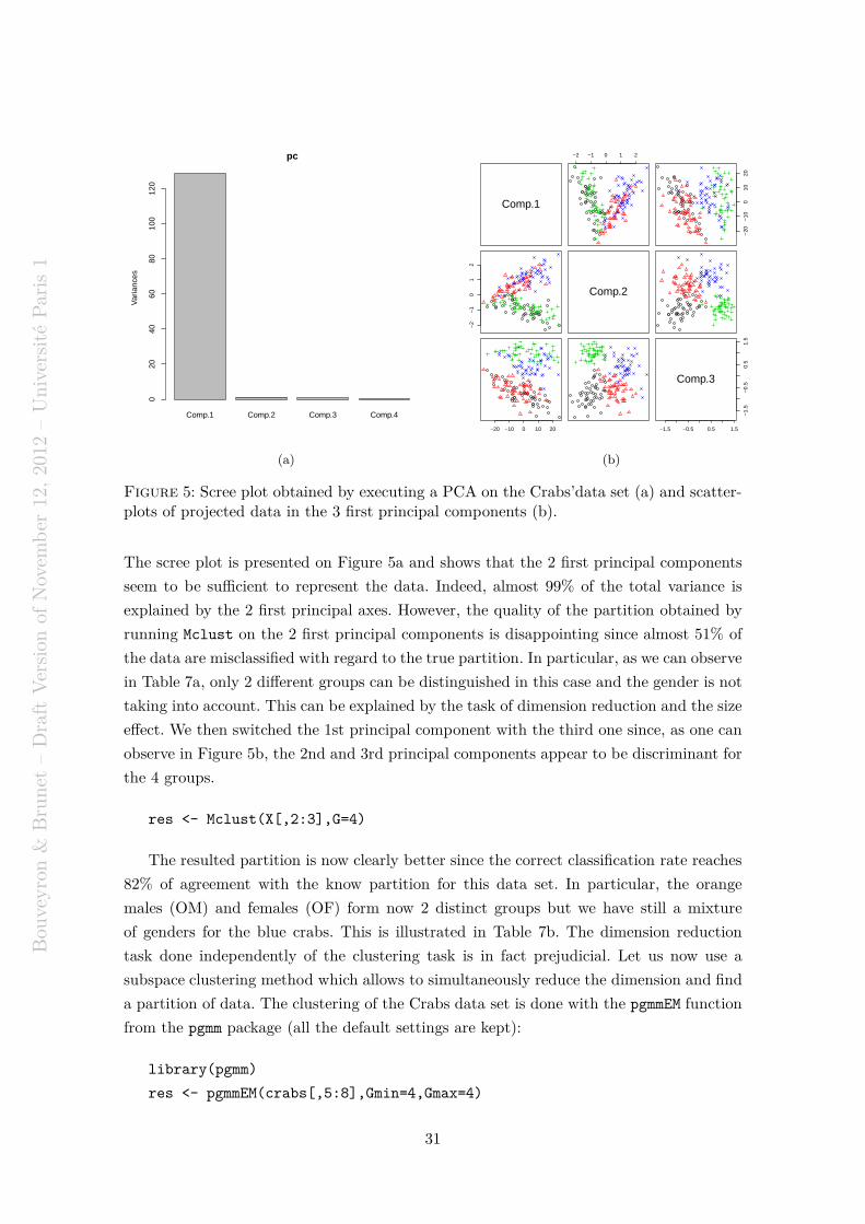
Bou

veyro

n&

Bru

net

–D

raft

Ver

sion

ofN

ovem

ber

12,

2012

–U

niv

ersi

téP

aris

1

Comp.1 Comp.2 Comp.3 Comp.4

pc

Var

ianc

es

020

4060

8010

012

0

(a)

Comp.1

−2 −1 0 1 2

−20

−10

010

20

−2

−1

01

2

Comp.2

−20 −10 0 10 20 −1.5 −0.5 0.5 1.5

−1.

5−

0.5

0.5

1.5

Comp.3

(b)

Figure 5: Scree plot obtained by executing a PCA on the Crabs’data set (a) and scatter-plots of projected data in the 3 first principal components (b).

The scree plot is presented on Figure 5a and shows that the 2 first principal components

seem to be sufficient to represent the data. Indeed, almost 99% of the total variance is

explained by the 2 first principal axes. However, the quality of the partition obtained by

running Mclust on the 2 first principal components is disappointing since almost 51% of

the data are misclassified with regard to the true partition. In particular, as we can observe

in Table 7a, only 2 different groups can be distinguished in this case and the gender is not

taking into account. This can be explained by the task of dimension reduction and the size

effect. We then switched the 1st principal component with the third one since, as one can

observe in Figure 5b, the 2nd and 3rd principal components appear to be discriminant for

the 4 groups.

res <- Mclust(X[,2:3],G=4)

The resulted partition is now clearly better since the correct classification rate reaches

82% of agreement with the know partition for this data set. In particular, the orange

males (OM) and females (OF) form now 2 distinct groups but we have still a mixture

of genders for the blue crabs. This is illustrated in Table 7b. The dimension reduction

task done independently of the clustering task is in fact prejudicial. Let us now use a

subspace clustering method which allows to simultaneously reduce the dimension and find

a partition of data. The clustering of the Crabs data set is done with the pgmmEM function

from the pgmm package (all the default settings are kept):

library(pgmm)

res <- pgmmEM(crabs[,5:8],Gmin=4,Gmax=4)

31

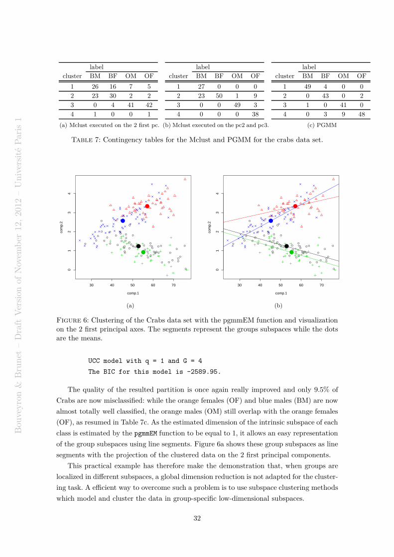
Bou

veyro

n&

Bru

net

–D

raft

Ver

sion

ofN

ovem

ber

12,

2012

–U

niv

ersi

téP

aris

1

label

cluster BM BF OM OF

1 26 16 7 5

2 23 30 2 2

3 0 4 41 42

4 1 0 0 1

(a) Mclust executed on the 2 first pc.

label

cluster BM BF OM OF

1 27 0 0 0

2 23 50 1 9

3 0 0 49 3

4 0 0 0 38

(b) Mclust executed on the pc2 and pc3.

label

cluster BM BF OM OF

1 49 4 0 0

2 0 43 0 2

3 1 0 41 0

4 0 3 9 48

(c) PGMM

Table 7: Contingency tables for the Mclust and PGMM for the crabs data set.

30 40 50 60 70

01

23

4

comp.1

com

p.2

(a)

30 40 50 60 70

01

23

4

comp.1

com

p.2

(b)

Figure 6: Clustering of the Crabs data set with the pgmmEM function and visualizationon the 2 first principal axes. The segments represent the groups subspaces while the dotsare the means.

UCC model with q = 1 and G = 4

The BIC for this model is -2589.95.

The quality of the resulted partition is once again really improved and only 9.5% of

Crabs are now misclassified: while the orange females (OF) and blue males (BM) are now

almost totally well classified, the orange males (OM) still overlap with the orange females

(OF), as resumed in Table 7c. As the estimated dimension of the intrinsic subspace of each

class is estimated by the pgmmEM function to be equal to 1, it allows an easy representation

of the group subspaces using line segments. Figure 6a shows these group subspaces as line

segments with the projection of the clustered data on the 2 first principal components.

This practical example has therefore make the demonstration that, when groups are

localized in different subspaces, a global dimension reduction is not adapted for the cluster-

ing task. A efficient way to overcome such a problem is to use subspace clustering methods

which model and cluster the data in group-specific low-dimensional subspaces.

32

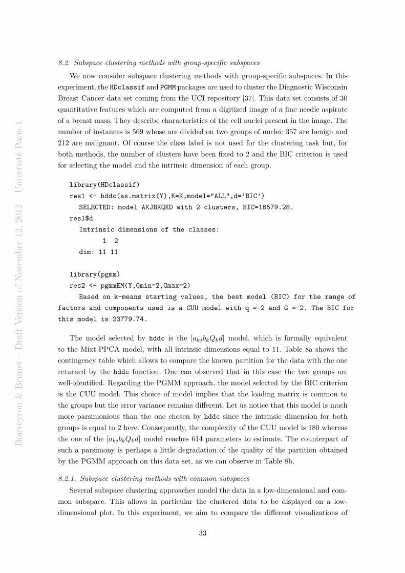
Bou

veyro

n&

Bru

net

–D

raft

Ver

sion

ofN

ovem

ber

12,

2012

–U

niv

ersi

téP

aris

1

8.2. Subspace clustering methods with group-specific subspaces

We now consider subspace clustering methods with group-specific subspaces. In this

experiment, the HDclassif and PGMM packages are used to cluster the Diagnostic Wisconsin

Breast Cancer data set coming from the UCI repository [37]. This data set consists of 30

quantitative features which are computed from a digitized image of a fine needle aspirate

of a breast mass. They describe characteristics of the cell nuclei present in the image. The

number of instances is 569 whose are divided on two groups of nuclei: 357 are benign and

212 are malignant. Of course the class label is not used for the clustering task but, for

both methods, the number of clusters have been fixed to 2 and the BIC criterion is used

for selecting the model and the intrinsic dimension of each group.

library(HDclassif)

res1 <- hddc(as.matrix(Y),K=K,model="ALL",d=’BIC’)

SELECTED: model AKJBKQKD with 2 clusters, BIC=16579.28.

res1$d

Intrinsic dimensions of the classes:

1 2

dim: 11 11

library(pgmm)

res2 <- pgmmEM(Y,Gmin=2,Gmax=2)

Based on k-means starting values, the best model (BIC) for the range of

factors and components used is a CUU model with q = 2 and G = 2. The BIC for

this model is 23779.74.

The model selected by hddc is the [akjbkQkd] model, which is formally equivalent

to the Mixt-PPCA model, with all intrinsic dimensions equal to 11. Table 8a shows the

contingency table which allows to compare the known partition for the data with the one

returned by the hddc function. One can observed that in this case the two groups are

well-identified. Regarding the PGMM approach, the model selected by the BIC criterion

is the CUU model. This choice of model implies that the loading matrix is common to

the groups but the error variance remains different. Let us notice that this model is much

more parsimonious than the one chosen by hddc since the intrinsic dimension for both

groups is equal to 2 here. Consequently, the complexity of the CUU model is 180 whereas

the one of the [akjbkQkd] model reaches 614 parameters to estimate. The counterpart of

such a parsimony is perhaps a little degradation of the quality of the partition obtained

by the PGMM approach on this data set, as we can observe in Table 8b.

8.2.1. Subspace clustering methods with common subspaces

Several subspace clustering approaches model the data in a low-dimensional and com-

mon subspace. This allows in particular the clustered data to be displayed on a low-

dimensional plot. In this experiment, we aim to compare the different visualizations of

33

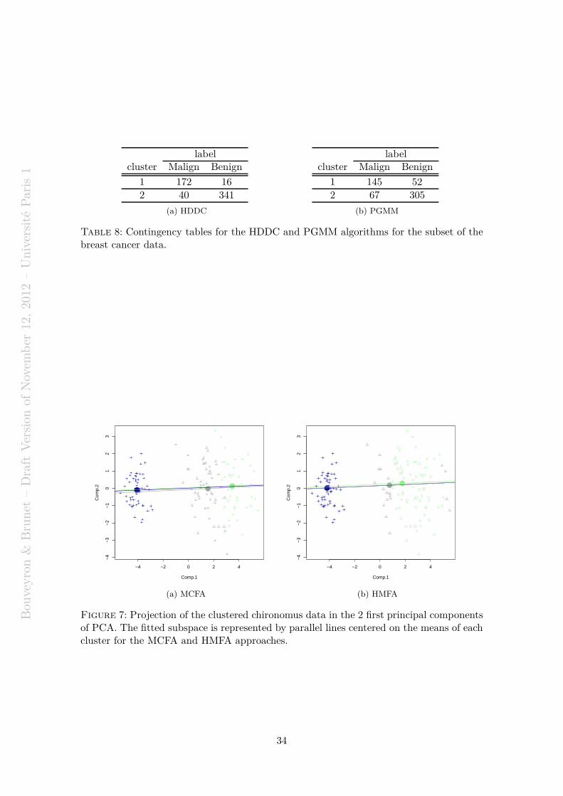
Bou

veyro

n&

Bru

net

–D

raft

Ver

sion

ofN

ovem

ber

12,

2012

–U

niv

ersi

téP

aris

1

labelcluster Malign Benign

1 172 16

2 40 341

(a) HDDC

labelcluster Malign Benign

1 145 52

2 67 305

(b) PGMM

Table 8: Contingency tables for the HDDC and PGMM algorithms for the subset of thebreast cancer data.

−4 −2 0 2 4

−4

−3

−2

−1

01

23

Comp.1

Com

p.2

(a) MCFA

−4 −2 0 2 4

−4

−3

−2

−1

01

23

Comp.1

Com

p.2

(b) HMFA

Figure 7: Projection of the clustered chironomus data in the 2 first principal componentsof PCA. The fitted subspace is represented by parallel lines centered on the means of eachcluster for the MCFA and HMFA approaches.

34

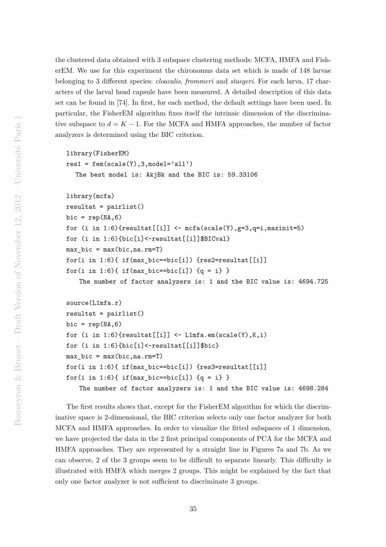
Bou

veyro

n&

Bru

net

–D

raft

Ver

sion

ofN

ovem

ber

12,

2012

–U

niv

ersi

téP

aris

1

the clustered data obtained with 3 subspace clustering methods: MCFA, HMFA and Fish-

erEM. We use for this experiment the chironomus data set which is made of 148 larvae

belonging to 3 different species: cloacalis, frommeri and staegeri. For each larva, 17 char-

acters of the larval head capsule have been measured. A detailed description of this data

set can be found in [74]. In first, for each method, the default settings have been used. In

particular, the FisherEM algorithm fixes itself the intrinsic dimension of the discrimina-

tive subspace to d = K − 1. For the MCFA and HMFA approaches, the number of factor

analyzers is determined using the BIC criterion.

library(FisherEM)

res1 = fem(scale(Y),3,model=’all’)

The best model is: AkjBk and the BIC is: 59.33106

library(mcfa)

resultat = pairlist()

bic = rep(NA,6)

for (i in 1:6)resultat[[i]] <- mcfa(scale(Y),g=3,q=i,maxinit=5)

for (i in 1:6)bic[i]<-resultat[[i]]$BICval

max_bic = max(bic,na.rm=T)

for(i in 1:6) if(max_bic==bic[i]) res2=resultat[[i]]

for(i in 1:6) if(max_bic==bic[i]) q = i

The number of factor analyzers is: 1 and the BIC value is: 4694.725

source(L1mfa.r)

resultat = pairlist()

bic = rep(NA,6)

for (i in 1:6)resultat[[i]] <- L1mfa.em(scale(Y),K,i)

for (i in 1:6)bic[i]<-resultat[[i]]$bic

max_bic = max(bic,na.rm=T)

for(i in 1:6) if(max_bic==bic[i]) res3=resultat[[i]]

for(i in 1:6) if(max_bic==bic[i]) q = i

The number of factor analyzers is: 1 and the BIC value is: 4698.284

The first results shows that, except for the FisherEM algorithm for which the discrim-

inative space is 2-dimensional, the BIC criterion selects only one factor analyzer for both

MCFA and HMFA approaches. In order to visualize the fitted subspaces of 1 dimension,

we have projected the data in the 2 first principal components of PCA for the MCFA and

HMFA approaches. They are represented by a straight line in Figures 7a and 7b. As we

can observe, 2 of the 3 groups seem to be difficult to separate linearly. This difficulty is

illustrated with HMFA which merges 2 groups. This might be explained by the fact that

only one factor analyzer is not sufficient to discriminate 3 groups.

35

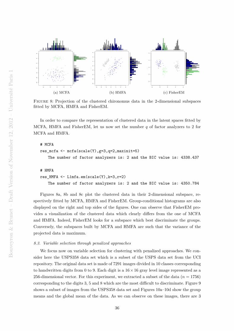
Bou

veyro

n&

Bru

net

–D

raft

Ver

sion

ofN

ovem

ber

12,

2012

–U

niv

ersi

téP

aris

1

−4 −2 0 2 4

−6

−4

−2

02

46

x[, 2

]

(a) MCFA

−3 −2 −1 0 1 2 3

−4

−3

−2

−1

01

23

x[, 2

]

(b) HMFA

−4 −2 0 2 4

−2

−1

01

2

x[,2

]

(c) FisherEM

Figure 8: Projection of the clustered chironomus data in the 2-dimensional subspacesfitted by MCFA, HMFA and FisherEM.

In order to compare the representation of clustered data in the latent spaces fitted by

MCFA, HMFA and FisherEM, let us now set the number q of factor analyzers to 2 for

MCFA and HMFA.

# MCFA

res_mcfa <- mcfa(scale(Y),g=3,q=2,maxinit=5)

The number of factor analyzers is: 2 and the BIC value is: 4338.437

# HMFA

res_HMFA <- L1mfa.em(scale(Y),k=3,r=2)

The number of factor analyzers is: 2 and the BIC value is: 4350.784

Figures 8a, 8b and 8c plot the clustered data in their 2-dimensional subspace, re-

spectively fitted by MCFA, HMFA and FisherEM. Group-conditional histograms are also

displayed on the right and top sides of the figures. One can observe that FisherEM pro-

vides a visualization of the clustered data which clearly differs from the one of MCFA

and HMFA. Indeed, FisherEM looks for a subspace which best discriminate the groups.

Conversely, the subspaces built by MCFA and HMFA are such that the variance of the

projected data is maximum.

8.3. Variable selection through penalized approaches

We focus now on variable selection for clustering with penalized approaches. We con-

sider here the USPS358 data set which is a subset of the USPS data set from the UCI

repository. The original data set is made of 7291 images divided in 10 classes corresponding

to handwritten digits from 0 to 9. Each digit is a 16× 16 gray level image represented as a

256-dimensional vector. For this experiment, we extracted a subset of the data (n = 1756)

corresponding to the digits 3, 5 and 8 which are the most difficult to discriminate. Figure 9

shows a subset of images from the USPS358 data set and Figures 10a–10d show the group

means and the global mean of the data. As we can observe on these images, there are 3

36

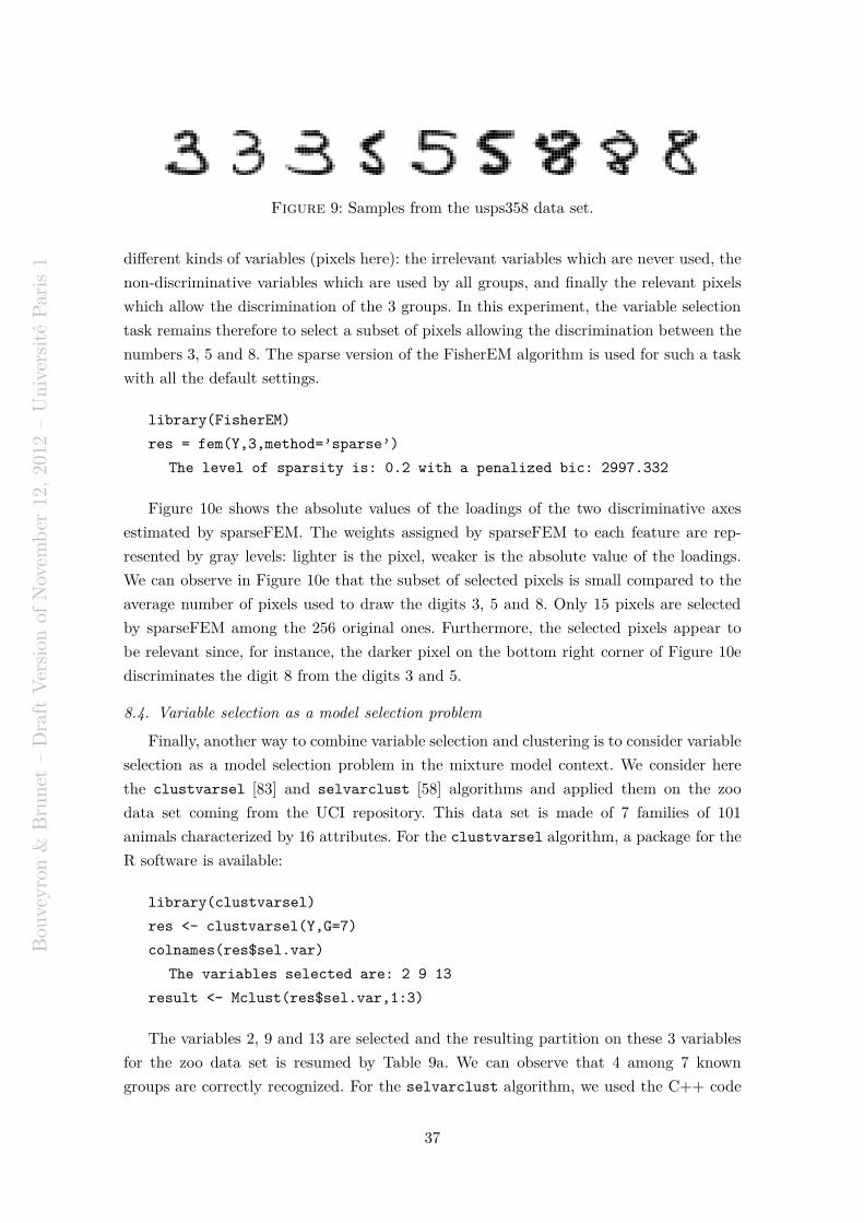
Bou

veyro

n&

Bru

net

–D

raft

Ver

sion

ofN

ovem

ber

12,

2012

–U

niv

ersi

téP

aris

1

Figure 9: Samples from the usps358 data set.

different kinds of variables (pixels here): the irrelevant variables which are never used, the

non-discriminative variables which are used by all groups, and finally the relevant pixels

which allow the discrimination of the 3 groups. In this experiment, the variable selection

task remains therefore to select a subset of pixels allowing the discrimination between the

numbers 3, 5 and 8. The sparse version of the FisherEM algorithm is used for such a task

with all the default settings.

library(FisherEM)

res = fem(Y,3,method=’sparse’)

The level of sparsity is: 0.2 with a penalized bic: 2997.332

Figure 10e shows the absolute values of the loadings of the two discriminative axes

estimated by sparseFEM. The weights assigned by sparseFEM to each feature are rep-

resented by gray levels: lighter is the pixel, weaker is the absolute value of the loadings.

We can observe in Figure 10e that the subset of selected pixels is small compared to the

average number of pixels used to draw the digits 3, 5 and 8. Only 15 pixels are selected

by sparseFEM among the 256 original ones. Furthermore, the selected pixels appear to

be relevant since, for instance, the darker pixel on the bottom right corner of Figure 10e

discriminates the digit 8 from the digits 3 and 5.

8.4. Variable selection as a model selection problem

Finally, another way to combine variable selection and clustering is to consider variable

selection as a model selection problem in the mixture model context. We consider here

the clustvarsel [83] and selvarclust [58] algorithms and applied them on the zoo

data set coming from the UCI repository. This data set is made of 7 families of 101

animals characterized by 16 attributes. For the clustvarsel algorithm, a package for the

R software is available:

library(clustvarsel)

res <- clustvarsel(Y,G=7)

colnames(res$sel.var)

The variables selected are: 2 9 13

result <- Mclust(res$sel.var,1:3)

The variables 2, 9 and 13 are selected and the resulting partition on these 3 variables

for the zoo data set is resumed by Table 9a. We can observe that 4 among 7 known

groups are correctly recognized. For the selvarclust algorithm, we used the C++ code

37

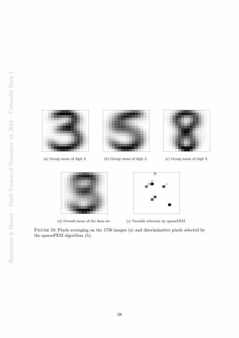
Bou

veyro

n&

Bru

net

–D

raft

Ver

sion

ofN

ovem

ber

12,

2012

–U

niv

ersi

téP

aris

1

(a) Group mean of digit 3 (b) Group mean of digit 5 (c) Group mean of digit 8

(d) Overall mean of the data set (e) Variable selection by sparseFEM

Figure 10: Pixels averaging on the 1756 images (a) and discriminative pixels selected bythe sparseFEM algorithm (b).

38

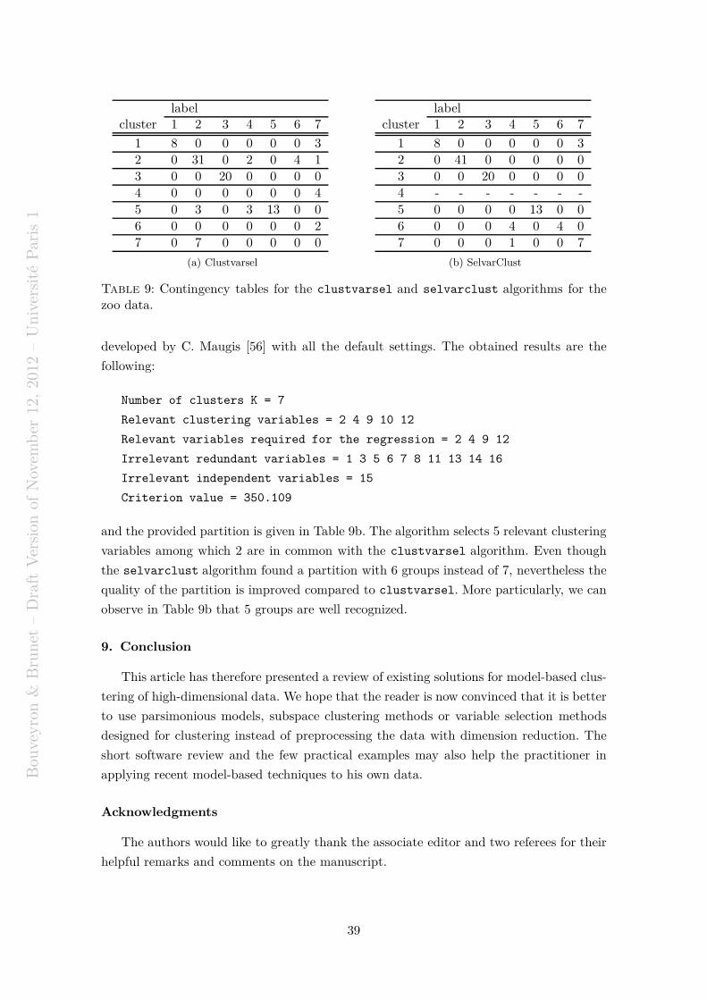
Bou

veyro

n&

Bru

net

–D

raft

Ver

sion

ofN

ovem

ber

12,

2012

–U

niv

ersi

téP

aris

1

labelcluster 1 2 3 4 5 6 7

1 8 0 0 0 0 0 3

2 0 31 0 2 0 4 1

3 0 0 20 0 0 0 0

4 0 0 0 0 0 0 4

5 0 3 0 3 13 0 0

6 0 0 0 0 0 0 2

7 0 7 0 0 0 0 0

(a) Clustvarsel

labelcluster 1 2 3 4 5 6 7

1 8 0 0 0 0 0 3

2 0 41 0 0 0 0 0

3 0 0 20 0 0 0 0

4 - - - - - - -

5 0 0 0 0 13 0 0

6 0 0 0 4 0 4 0

7 0 0 0 1 0 0 7

(b) SelvarClust

Table 9: Contingency tables for the clustvarsel and selvarclust algorithms for thezoo data.

developed by C. Maugis [56] with all the default settings. The obtained results are the

following:

Number of clusters K = 7

Relevant clustering variables = 2 4 9 10 12

Relevant variables required for the regression = 2 4 9 12

Irrelevant redundant variables = 1 3 5 6 7 8 11 13 14 16

Irrelevant independent variables = 15

Criterion value = 350.109

and the provided partition is given in Table 9b. The algorithm selects 5 relevant clustering

variables among which 2 are in common with the clustvarsel algorithm. Even though

the selvarclust algorithm found a partition with 6 groups instead of 7, nevertheless the

quality of the partition is improved compared to clustvarsel. More particularly, we can

observe in Table 9b that 5 groups are well recognized.

9. Conclusion

This article has therefore presented a review of existing solutions for model-based clus-

tering of high-dimensional data. We hope that the reader is now convinced that it is better

to use parsimonious models, subspace clustering methods or variable selection methods

designed for clustering instead of preprocessing the data with dimension reduction. The

short software review and the few practical examples may also help the practitioner in

applying recent model-based techniques to his own data.

Acknowledgments

The authors would like to greatly thank the associate editor and two referees for their

helpful remarks and comments on the manuscript.

39

Bou

veyro

n&

Bru

net

–D

raft

Ver

sion

ofN

ovem

ber

12,

2012

–U

niv

ersi

téP

aris

1

References

[1] R. Agrawal, J. Gehrke, D. Gunopulos, and P. Raghavan. Automatic subspace clus-

tering of high-dimensional data for data mining application. In ACM SIGMOD

International Conference on Management of Data, pages 94–105, 1998.

[2] J. L. Andrews and P. D. McNicholas. Extending mixtures of multivariate t-factor

analyzers. Statistics and Computing, 21(3):361–373, 2011.

[3] J.L. Andrews and P.D. McNicholas. Model-based clustering, classification, and dis-

criminant analysis via mixtures of multivariate t-distributions. Statistics and Com-

puting, 22(5):1021–1029, 2012.

[4] J. Baek, G. McLachlan, and L. Flack. Mixtures of Factor Analyzers with Com-

mon Factor Loadings: Applications to the Clustering and Visualisation of High-

Dimensional Data. IEEE Transactions on Pattern Analysis and Machine Intelli-

gence, pages 1–13, 2009.

[5] J. Banfield and A. Raftery. Model-based Gaussian and non-Gaussian clustering.

Biometrics, 49:803–821, 1993.

[6] R. Bellman. Dynamic Programming. Princeton University Press, 1957.

[7] L. Bergé, C. Bouveyron, and S. Girard. HDclassif : an R Package for Model-Based

Clustering and Discriminant Analysis of High-Dimensional Data. Journal of Statis-

tical Software, 42(6):1–29, 2012.

[8] P.J. Bickel and E. Levina. Covariance regularization by thresholding. Annals of

Statistics, 36:2577–2604, 2008.

[9] P.J. Bickel and E. Levina. Regularized estimation of large covariance matrices.

Annals of Statistics, 36:199–227, 2008.

[10] C. Biernacki, G. Celeux, and G. Govaert. Assessing a mixture model for clustering

with the integrated completed likelihood. IEEE Transactions on Pattern Analysis

and Machine Intelligence, 22(7):719–725, 2001.

[11] C. Biernacki, G. Celeux, G. Govaert, and F. Langrognet. Model-based cluster and

discriminant analysis with the mixmod software. Computational Statistics and Data

Analysis, 51:587–600, 2006.

[12] C. Bishop. Pattern recognition and machine learning. Springer, New York, 2006.

[13] G. Bouchard and C. Bouveyron. The statlearn toolbox: statistical learning tools for

Matlab, 2007. http://statlearn.free.fr/.

[14] G. Bouchard and G. Celeux. Model selection in supervised classification. Transac-

tions on Pattern Analysis and Machine Intelligence, 28(4):544–554, 2005.

40

Bou

veyro

n&

Bru

net

–D

raft

Ver

sion

ofN

ovem

ber

12,

2012

–U

niv

ersi

téP

aris

1

[15] C. Bouveyron and C. Brunet. On the estimation of the latent discriminative sub-

space in the Fisher-EM algorithm. Journal de la Société Francaise de Statistique,

152(3):98–115, 2011.

[16] C. Bouveyron and C. Brunet. Discriminative variable selection for clustering with the

sparse Fisher-EM algorithm. Technical Report Preprint HAL 00685183, Laboratoire

SAMM, Université Paris 1 Panthéon-Sorbonne, 2012.

[17] C. Bouveyron and C. Brunet. Simultaneous model-based clustering and visualization

in the Fisher discriminative subspace. Statistics and Computing, 22(1):301–324,

2012.

[18] C. Bouveyron and C. Brunet. Theoretical and practical considerations on the con-

vergence properties of the Fisher-EM algorithm. Journal of Multivariate Analysis,

109:29–41, 2012.

[19] C. Bouveyron, G. Celeux, and S. Girard. Intrinsic Dimension Estimation by Max-

imum Likelihood in Isotropic Probabilistic PCA. Pattern Recognition Letters,

32(14):1706–1713, 2011.

[20] C. Bouveyron, S. Girard, and C. Schmid. High-Dimensional Data Clustering. Com-

putational Statistics and Data Analysis, 52(1):502–519, 2007.

[21] C. Bouveyron, S. Girard, and C. Schmid. High Dimensional Discriminant Analysis.

Communications in Statistics : Theory and Methods, 36(14):2607–2623, 2007.

[22] N. Campbell and Mahon R.J. A multivariate study of variation in two species of

rock crabs of genus Leptograpsus. Australian Journal of Zoology, 22:417–425, 1974.

[23] R. Cattell. The scree test for the number of factors. Multivariate Behavioral Re-

search, 1(2):145–276, 1966.

[24] G. Celeux and G. Govaert. Gaussian parsimonious clustering models. Pattern Recog-

nition, 28:781–793, 1995.

[25] G. Celeux, M.-L. Martin-Magniette, C. Maugis, and A. Raftery. Letter to the editor.

Journal of the American Statistical Association, 106(493), 2011.

[26] W.C. Chang. On using principal component before separating a mixture of two

multivariate normal distributions. Journal of the Royal Statistical Society, Series C,

32(3):267–275, 1983.

[27] W.-C. Chen and G. Ostrouchov. Parallel Model-Based Clustering. Oak Ridge Na-

tional Laboratory, Oak Ridge, TN, USA, 2012.

[28] A. Dempster, N. Laird, and D. Robin. Maximum likelihood from incomplete data

via the EM algorithm. Journal of the Royal Statistical Society, 39(1):1–38, 1977.

41

Bou

veyro

n&

Bru

net

–D

raft

Ver

sion

ofN

ovem

ber

12,

2012

–U

niv

ersi

téP

aris

1

[29] R. Duda, P. Hart, and D. Stork. Pattern classification. John Wiley & Sons, 2000.

[30] B. Efron, T. Hastie, I. Johnstone, and R. Tibshirani. Least angle regression. Annals

of Statistics, 32:407–499, may 2004.

[31] R.A. Fisher. The use of multiple measurements in taxonomic problems. Annals of

Eugenics, 7:179–188, 1936.

[32] D.H. Foley and J.W. Sammon. An optimal set of discriminant vectors. IEEE Trans-

actions on Computers, 24:281–289, 1975.

[33] C. Fraley. Algorithms for model-based Gaussian Hierarchical Clustering. SIAM

Journal on Scientific Computing, 20:270–281, 1998.

[34] C. Fraley and A. Raftery. MCLUST: Software for Model-Based Cluster Analysis.

Journal of Classification, 16:297–306, 1999.

[35] C. Fraley and A. Raftery. Model-based clustering, discriminant analysis, and density

estimation. Journal of the American Statistical Association, 97(458), 2002.

[36] Browne-R.P. Franczak, B.C. and P.D. McNicholas. Mixtures of shifted asymmetric

Laplace distributions. Technical Report Preprint arXiv:1207.1727v2, University of

Guelph, 2012.

[37] A. Frank and A. Asuncion. UCI Machine Learning Repository, 2010.

http://archive.ics.uci.edu/ml.

[38] J. Friedman, T. Hastie, and R. Tibshirani. Sparse inverse covariance estimation with

the graphical lasso. Journal of the American Statistical Association, 104:177–186,

2008.

[39] J.H. Friedman. Regularized discriminant analysis. The Journal of the American

Statistical Association, 84:165–175, 1989.

[40] K. Fukunaga. Introduction to Statistical Pattern Recognition. Academic. Press, San

Diego, 1990.

[41] G. Galimberti, A. Montanari, and C. Viroli. Penalized factor mixture analysis for

variable selection in clustered data. Computational Statistics and Data Analysis,

53(12):4301–4310, oct 2009.

[42] G. Galimberti and G. Soffritti. Using conditional independence for parsimonious

model-based Gaussian clustering. Statistics and Computing, page in press, 2012.

[43] Z. Ghahramani and G.E. Hinton. The EM algorithm for factor analyzers. Technical

report, University of Toronto, 1997.

42

Bou

veyro

n&

Bru

net

–D

raft

Ver

sion

ofN

ovem

ber

12,

2012

–U

niv

ersi

téP

aris

1

[44] P. Hall, J. Marron, and A. Neeman. Geometric representation of high dimension, low

sample size data. Journal of the Royal Statistical Society, Serie B, 67(3):427–444,

2005.

[45] T. Hastie, A. Buja, and R. Tibshirani. Penalized discriminant analysis. Annals of

Statistics, 23:73–102, 1995.

[46] H. Hotelling. Analysis of a complex of statistical variables into principal components.

Journal of Educational Psychology, 24:417–441, 1933.

[47] P. Huber. Projection pursuit. The Annals of Statistics, 13(2):435–525, 1985.

[48] N. El Karoui. Operator norm consistent estimation of large dimensional sparse

covariance matrices. Technical report 734, UC Berkeley, Department of Statistics,

2007.

[49] M. Law, M. Figueiredo, and A. Jain. Simultaneous Feature Selection and Clustering

Using Mixture Models. IEEE Trans. on PAMI, 26(9):1154–1166, 2004.

[50] O. Ledoit and M. Wolf. A well-conditioned estimator for large-dimensional covari-

ance matrices. Journal of Multivariate Analysis, 88:365–411, 2003.

[51] S. Lee and G.J. McLachlan. Finite mixtures of multivariate skew t-distributions:

some recent and new results. Statistics and Computing, to appear, 2013.

[52] T. Lin, J. Lee, and S. Yen. Finite mixture modelling using the skew normal distri-

bution. Statistica Sinica, 17:909–927, 2007.

[53] B.G. Lindsay. Mixture models: Theory, geometry and applications. In NSF- CBMS

Regional Conference Series in Probability and Statistics, volume 5. Institute of Math-

ematical Statistics, 1995.

[54] J. Liu, J.L. Zhang, M.J. Palumbo, and C.E. Lawrence. Bayesian clustering with

variable and transformation selection. Bayesian Statistics, 7:249–276, 2003.

[55] J. MacQueen. Some methods for classification and analysis of multivariate observa-

tions. In L.M. Cam and J. Neyman, editors, Proceedings of the 5th Berkeley sympo-

sium on mathematical statistics and probability, volume 1, pages 281–297. University

of California Press, 1967.

[56] C. Maugis. The selvarclust software, 2009.

http://www.math.univ-toulouse.fr/~maugis/SelvarClustHomepage.html.

[57] C. Maugis, G. Celeux, and M.-L. Martin-Magniette. Variable selection for Clustering

with Gaussian Mixture Models. Biometrics, 65(3):701–709, 2009.

43

Bou

veyro

n&

Bru

net

–D

raft

Ver

sion

ofN

ovem

ber

12,

2012

–U

niv

ersi

téP

aris

1

[58] C. Maugis, G. Celeux, and M.-L. Martin-Magniette. Variable selection in model-

based clustering: A general variable role modeling. Computational Statistics and

Data Analysis, 53:3872–3882, 2009.

[59] G. McLachlan. The EMMIX-MFA software, 2003.

http://www.maths.uq.edu.au/~gjm/mix_soft/mfa/.

[60] G. McLachlan. The EMMIX software, 2010.

http://www.maths.uq.edu.au/~gjm/mix_soft/EMMIX_R/index.html.

[61] G. McLachlan. The mcfa function for the R software, 2010.

http://www.maths.uq.edu.au/~gjm/mix_soft/mcfa/.

[62] G. McLachlan and K.E. Basford. Mixture models : inference and applications to

clustering. New York: Marcel Dekker, 1988.

[63] G. McLachlan and T. Krishnan. The EM algorithm and extensions. Wiley Inter-

science, New York, 1997.

[64] G. McLachlan and D. Peel. Finite Mixture Models. Wiley Interscience, New York,

2000.

[65] G. McLachlan, D. Peel, and R. Bean. Modelling high-dimensional data by mixtures

of factor analyzers. Computational Statistics and Data Analysis, (41):379, 2003.

[66] G. J. McLachlan, R. W. Bean, and L. Ben-Tovim Jones. Extension of the mixture of

factor analyzers model to incorporate the multivariate t-distribution. Computational

Statistics and Data Analysis, 51:5327–5338, 2011.

[67] G.J. McLachlan, D. Peel, K.E. Basford, and P. Adams. The emmix software for the

fitting of mixtures of normal t-components. Journal of Statistical Software, 4(2):1–

14, 1999.

[68] J.G. McLachlan and D. Peel. Robust cluster analysis via mixtures of multivariate

t-distributions. In Lecture Notes in Computer Science, 1451:658–666, 1998.

[69] P. McNicholas and B. Murphy. Parsimonious Gaussian mixture models. Statistics

and Computing, 18(3):285–296, 2008.

[70] P. McNicholas and B. Murphy. Model-based clustering of microarray expression

data via latent gaussian mixture models. Bioinformatics, 26(21):2705–2712, 2010.

[71] X-L. Meng and D. Van Dyk. The EM algorithm - an old folk song sung to a fast

new tune. Journal of the Royal Statistical Society, Series B, 59(3):511–567, 1997.

[72] A. Mkhadri, G. Celeux, and A. Nasrollah. Regularization in discriminant analysis:

a survey. Computational Statistics and Data Analysis, 23:403–423, 1997.

44

Bou

veyro

n&

Bru

net

–D

raft

Ver

sion

ofN

ovem

ber

12,

2012

–U

niv

ersi

téP

aris

1

[73] C. Mo. emgm: EM algorithm for Gaussian mixture model, 2009.

http://www.mathworks.com/matlabcentral/fileexchange/26184.

[74] A. Montanari and C. Viroli. Heteroscedastic factor mixture analysis. Statistical

Modelling, 10(4):441–460, 2010.

[75] F. Murtagh. The remarkable simplicity of very high dimensional data: application

of model-based clustering. Journal of Classification, 26:249–277, 2009.

[76] F. Murtagh and A.E. Raftery. Fitting straight lines to point patterns. Pattern

Recognition, 17:479–483, 1984.

[77] V. Partovi Nia and A. C. Davison. High-Dimensional Bayesian Clustering with

Variable Selection: The R Package bclust. Journal of Statistical Software, 47(5):1–

22, 2012.

[78] W. Pan and X. Shen. Penalized model-based clustering with application to variable

selection. Journal of Machine Learning Research, 8:1145–1164, 2007.

[79] L. Parsons, E. Haque, and H. Liu. Subspace clustering for high-dimensional data: a

review. SIGKDD Explor. Newsl., 6(1):69–76, 1998.

[80] T. Pavlenko. On feature selection, curse of dimensionality and error probability in

discriminant analysis. Journal of Statistical Planning and Inference, 115:565–584,

2003.

[81] T. Pavlenko and D. Von Rosen. Effect of dimensionality on discrimination. Statistics,

35(3):191–213, 2001.

[82] K. Pearson. On lines and planes of closest fit to systems of points in space. Philo-

sophical Magazine, 6(2):559–572, 1901.

[83] A. Raftery and N. Dean. Variable selection for model-based clustering. Journal of

the American Statistical Association, 101(473):168–178, 2006.

[84] D. Rubin and D. Thayer. EM algorithms for ML factor analysis. Psychometrika,

47(1):69–76, 1982.

[85] G. Sanguinetti. Dimensionality reduction of clustered datasets. IEEE Transactions

On Pattern Analysis And Machine Intelligence, 30(3):1–29, 2008.

[86] G. Schwarz. Estimating the dimension of a model. The Annals of Statistics, 6:461–

464, 1978.

[87] A.J. Scott and M.J. Symons. Clustering methods based on likelihood ratio criteria.

Biometrics, 27:387–397, 1971.

45

Bou

veyro

n&

Bru

net

–D

raft

Ver

sion

ofN

ovem

ber

12,

2012

–U

niv

ersi

téP

aris

1

[88] D. Scott and J. Thompson. Probability density estimation in higher dimensions. In

Fifteenth Symposium in the Interface, pages 173–179, 1983.

[89] L. Scrucca. Dimension Reduction for Model-Based Clustering. Statistics and Com-

puting, 20(4):471–484, 2010.

[90] C. Spearman. The proof and measurement of association between two things. Amer-

ican Journal of Psychology, 15:72–101, 1904.

[91] M. Tipping and C. Bishop. Probabilistic principal component analysis. Technical

Report NCRG-97-010, Neural Computing Research Group, Aston University, 1997.

[92] M. Tipping and C. Bishop. Mixtures of Probabilistic Principal Component Analy-

sers. Neural Computation, 11(2):443–482, 1999.

[93] W.N. Venables and B.D. Ripley. Modern Applied Statistics with S. Springer, 2002.

[94] C. Viroli. The hmfa function for the R software, 2010.

http://www2.stat.unibo.it/viroli/Cinzia_Viroli/Software_&_Data.html.

[95] C. Viroli. The mmfa function for the R software, 2010.

http://www2.stat.unibo.it/viroli/Software/MFMA_1.0.tar.gz.

[96] S. Wang and J. Zhou. Variable selection for model-based high dimensional clustering

and its application to microarray data. Biometrics, 64:440–448, 2008.

[97] J.H. Ward. Hierarchical groupings to optimize an objective function. Journal of the

American Statistical Association, 58:234–244, 1963.

[98] D.M. Witten and R. Tibshirani. A framework for feature selection in clustering.

Journal of the American Statistical Association, 105(490):713–726, 2010.

[99] J.H. Wolfe. Object cluster analysis of social areas. Master’s thesis, University of

California, Berkeley, 1963.

[100] C. Wu. On the convergence properties of the EM algorithm. Annals of Statistics,

11:95–103, 1983.

[101] B. Xie, W. Pan, and X. Shen. Penalized model-based clustering with cluster-specific

diagonal covariance matrices and grouped variables. Electrical Journal of Statistics,

2:168–212, 2008.

[102] B. Xie, W. Pan, and X. Shen. Penalized mixtures of factor analyzers with application

to clustering high-dimensional microarray data. Bioinformatics, 26(4):501–508, 2010.

[103] R. Yoshida, T. Higuchi, and S. Imoto. A mixed factor model for dimension reduction

and extraction of a group structure in gene expression data. IEEE Computational

Systems Bioinformatics Conference, 8:161–172, 2004.

46

Bou

veyro

n&

Bru

net

–D

raft

Ver

sion

ofN

ovem

ber

12,

2012

–U

niv

ersi

téP

aris

1

[104] R. Yoshida, T. Higuchi, S. Imoto, and S. Miyano. Array cluster: an analytic tool for

clustering, data visualization and model finder on gene expression profiles. Bioin-

formatics, 22:1538–1539, 2006.

[105] Z. Zhang, G. Dai, and M.I. Jordan. A flexible and efficient algorithm for regularized

fisher discriminant analysis. In Proceedings of the European Conference on Machine

Learning and Knowledge Discovery in Databases, pages 632–647, 2009.

47