PUB. IRMA, LILLE 2011

Vol. 71, No II

Model-based Clustering of Time Series

in Group-speci�c Functional Subspaces∗

Charles Bouveyron a, Julien Jacques b

Abstract

This work develops a general procedure for clustering functional datawhich adapts the e�cient clustering method HDDC, originally proposedin the multivariate context. The resulting clustering method, called fun-HDDC, is based on a functional latent mixture model which �ts the func-tional data in group-speci�c functional subspaces. By constraining modelparameters within and between groups, a family of parsimonious modelsis exhibited which allow to �t onto various situations. An estimation pro-cedure based on the EM algorithm is proposed for estimating both themodel parameters and the group-speci�c functional subspaces. Experi-ments on real-world datasets show that the proposed approach performsbetter or similarly than classical clustering methods while providing usefulinterpretations of the groups.

Résumé

Nous proposons dans cet article une procédure de classi�cation auto-matique de données fonctionnelles qui adapte la méthode HDDC conçueinitialement dans un cadre multivarié. La méthode de clustering résul-tante, appelée funHDDC, est basée sur un modèle de mélange latent fonc-tionnel qui modèlise les données dans des sous-espaces spéci�ques auxclasses. Une famille de modèles particuliers est dé�nie en spéci�ant descontraintes sur les paramètres du modèle. Une procèdure d'estimationbasée sur l'algorithme EM permet d'estimer à la fois les paramètres dumodèle et les sous-espaces spéci�ques aux classes. Des expérimentationssur données réelles illustrent l'intérêt de la méthode, tant d'un point devue performance de classement que d'un point de vue interprétabilité desrésultats.

MSC 2009 subject classi�cations. 62J99.

Key words and phrases. Functional data, time series clustering, model-basedclustering, group-speci�c functional subspaces, functional PCA.

∗Preprint.a Laboratoire SAMM, Université Paris I Panthéon-Sorbonne, Paris, France.b Laboratoire P. Painlevé, UMR 8524 CNRS Université Lille I, & INRIA Lille Nord Europe,

Cité Scienti�que, F-59655 Villeneuve d'Ascq Cedex, France.

II � 3

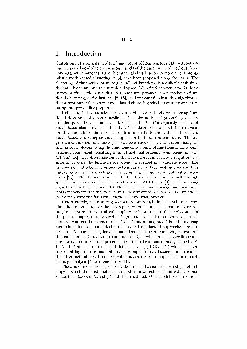
1 Introduction

Cluster analysis consists in identifying groups of homogeneous data without us-ing any prior knowledge on the group labels of the data. A lot of methods, fromnon-parametric k-means [10] or hierarchical classi�cation to more recent proba-bilistic model-based clustering [2, 6], have been proposed along the years. Theclustering of time series, or more generally of functions, is a di�cult task sincethe data live in an in�nite dimensional space. We refer for instance to [21] for asurvey on time series clustering. Although non-parametric approaches to func-tional clustering, as for instance [8, 18], lead to powerful clustering algorithms,the present paper focuses on model-based clustering which have moreover inter-esting interpretability properties.

Unlike the �nite dimensional cases, model-based methods for clustering func-tional data are not directly available since the notion of probability densityfunction generally does not exist for such data [7]. Consequently, the use ofmodel-based clustering methods on functional data consists usually in �rst trans-forming the in�nite dimensional problem into a �nite one and then in using amodel-based clustering method designed for �nite dimensional data. The ex-pression of functions in a �nite space can be carried out by either discretizing thetime interval, decomposing the functions onto a basis of functions or onto someprincipal components resulting from a functional principal component analysis(FPCA) [16]. The discretization of the time interval is usually straightforwardsince in practice the functions are already measured in a discrete scale. Thefunctions can also be decomposed onto a basis of well-de�ned functions such asnatural cubic splines which are very popular and enjoy some optimality prop-erties [20]. The decomposition of the functions can be done as well throughspeci�c time series models such as ARMA or GARCH (see [9] for a clusteringalgorithm based on such models). Note that in the case of using functional prin-cipal components, the functions have to be also expressed in a basis of functionsin order to solve the functional eigen-decomposition problem.

Unfortunately, the resulting vectors are often high-dimensional. In partic-ular, the discretization or the decomposition of the functions onto a spline ba-sis (for instance, 20 natural cubic splines will be used in the applications ofthe present paper) usually yield to high-dimensional datasets with sometimesless observations than dimensions. In such situations, model-based clusteringmethods su�er from numerical problems and regularized approaches have tobe used. Among the regularized model-based clustering methods, we can citethe parsimonious Gaussian mixture models [2, 6], which assume speci�c covari-ance structures, mixture of probabilistic principal component analyzers (MixtP-PCA, [19]) and high-dimensional data clustering (HDDC, [4]) which both as-sume that high-dimensional data live in group-speci�c subspaces. In particular,the latter method have been used with success in various application �elds suchas image analysis [4] or chemometry [11].

The clustering methods previously described all consist in a two-step method-ology in which the functional data are �rst transformed into a �nite dimensionalvector (the discretization step) and then clustered. Only model-based methods

II � 4

have been mentioned but some non-parametric methods such as k-means couldalso be considered. Unfortunately, these two-step approaches do separately thediscretization and the clustering steps, and this may lead to a loss of discrimina-tive information. Recently, a new approach due to James and Sugar [12] allowsthe interaction between the discretization and the clustering steps by introduc-ing a stochastic model onto the basis coe�cients. This approach is announcedto be particularly e�ective when the functional data are sparsely sampled. Inthe same spirit, we propose in the present paper to adapt the HDDC methodto functional data in order to model and cluster the functional data in group-speci�c subspaces of low dimensionality. The modeling of the functions of eachgroup in a speci�c subspace should, in addition to providing an interesting clus-tering of the data, ease the interpretation of the clustered data.

The paper is organized as follows. Section 2 presents the proposed func-tional latent mixture model as well as a family of parsimonious submodels andthe associated maximum likelihood estimation. Section 3 �rst proposes an in-troductory example in order to highlight the main features of the proposedmethod. A benchmark comparison with state-of-the-art methods is also pro-vided in Section 3 on real-world time series datasets. Finally, Section 4 providessome concluding remarks.

2 Model-based clustering in functional subspaces

This section introduces a family of latent mixture models designed for functionaldata which adapts the models of [4], proposed in the multivariate context. Modelinference and estimation of hyper-parameters are also discussed.

2.1 The functional latent mixture model

Let us consider a set of n observed time series or curves {x1, ..., xn}, wherexi = {xi(t)}t∈[0,T ] (1 ≤ i ≤ n), that one wants to cluster into K homogeneousgroups.

On the one hand, let us �rst assume that the observed curves are independentrealizations of a L2-continuous stochastic process X = {X(t)}t∈[0,T ] for whichthe sample paths, i.e. the observed curves xi, belong to L2[0, T ]. In practice,the functional expressions of the observed curves are not known and we onlyhave access to the discrete observations xij = xi(tij) at a �nite set of times{tij : j = 1, . . . ,mi}. As explained in [1], it is thus necessary to reconstructthe functional form of the data from their discrete observations. A commonway to do this is to consider that curves belong to a �nite dimensional spacespanned by a basis of functions (see, for example, [16]). Let us therefore considersuch a basis {ψ1, . . . , ψp} and assume that the stochastic process X admits thefollowing basis expansion:

X(t) =

p∑j=1

γjψj(t), (1)

II � 5

with γj ∈ R (j = 1, . . . , p) and where the number p of basis functions is assumedto be known and �xed. The basis expansion of each observed curve xi(t) =∑pj=1 γijψj(t) can be estimated by an interpolation procedure, if the curves are

observed without noise, or by least square smoothing, if they are observed witherror.

Let also assume that there exists an unobserved variable Z = (Z1, . . . , ZK) ∈{0, 1}K such that zik, the values of Zk for the curve xi, indicates if xi belongsto the kth group or not. The clustering task aims therefore to predict the valueof Z for each observed curve xi.

On the other hand, let us assume that there exist K functional latent sub-spaces E1[0, T ], ...,EK [0, T ] (Ek[0, T ] ⊂ L2[0, T ] for all k = 1, . . . ,K) where theobserved curves live conditionally to their group belonging. For each observedcurve xi, let yi be its latent representation which lives in Ek[0, T ] if zik = 1.We further assume that, in each group-speci�c functional subspace Ek, the la-tent time series yi, such that zik = 1, are also sample paths of a L2-continuousstochastic process Y = {Y (t)}t∈[0,T ] admitting a basis expansion depending onthe group at hand:

Y (t)|Zk=1 =

dk∑j=1

αkjψj(t),

where {ψj}j=1,dk is the same basis of functions as in Equation (1), but with apossible reduced number of functions dk (dk ≤ p), which becomes a parameterof the model.

We �nally assume that Y is linked to X, conditionally to Z, through a lineartransformation:

X|Zk=1 = UkY|Zk=1 + ε|Zk=1,

where Uk is a linear operator de�ned from L2[0, T ] to Ek[0, T ] and representedby a p × dk matrix Uk, and ε a noise function admitting the basis expansionε(t) =

∑pj=1 βjψj(t).

We now make some distributional assumptions on the stochastic processesX,Y and ε through their respective basis expansions. Firstly, the basis coe�cients{α1, ..., αn} of Y are assumed to be distributed, conditionally to Z, accordingto a multivariate Gaussian density:

α|Zk=1 ∼ N (mk, Sk),

where mk and Sk = diag(ak1, ..., akdk) are respectively the mean and the co-variance matrix of the kth group. Secondly, the basis coe�cients {β1, ..., βn} ofthe noise function ε are assumed as well to be distributed, conditionally to Z,according to a multivariate Gaussian density:

β|Zk=1 ∼ N (0,Γk).

With these distributional assumptions, the conditional distribution of the basiscoe�cients of X is:

γ|α,Zk=1 ∼ N (Ukα,Γk),

II � 6

and its marginal distribution is therefore a mixture of Gaussians:

p(γ) =

K∑k=1

πkφ(γ;µk,Σk),

where φ is the Gaussian density function, µk = Ukmk, Σk = UkSkUtk + Γk

and πk = P (Zk = 1) is the prior probability of group k. Let us also de�neQk = [Uk, Vk] a p× p matrix which satis�es QtkQk = QkQ

tk = Ip and for which

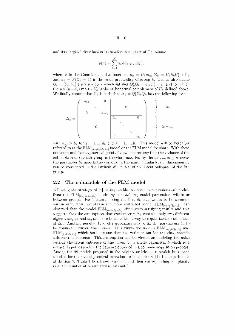
the p× (p− dk) matrix Vk is the orthonormal complement of Uk de�ned above.We �nally assume that Γk is such that ∆k = QtkΣkQk has the following form:

∆k =

ak1 0

. . .

0 akdk

0

0

bk 0

. . .

. . .

0 bk

dk

(p− dk)

with akj > bk for j = 1, ..., dk and k = 1, ...,K. This model will be hereafterreferred to as the FLM[akjbkQkdk] model or the FLM model for short. With thesenotations and from a practical point of view, one can say that the variance of theactual data of the kth group is therefore modeled by the ak1, ..., akdk whereasthe parameter bk models the variance of the noise. Similarly, the dimension dkcan be considered as the intrinsic dimension of the latent subspace of the kthgroup.

2.2 The submodels of the FLM model

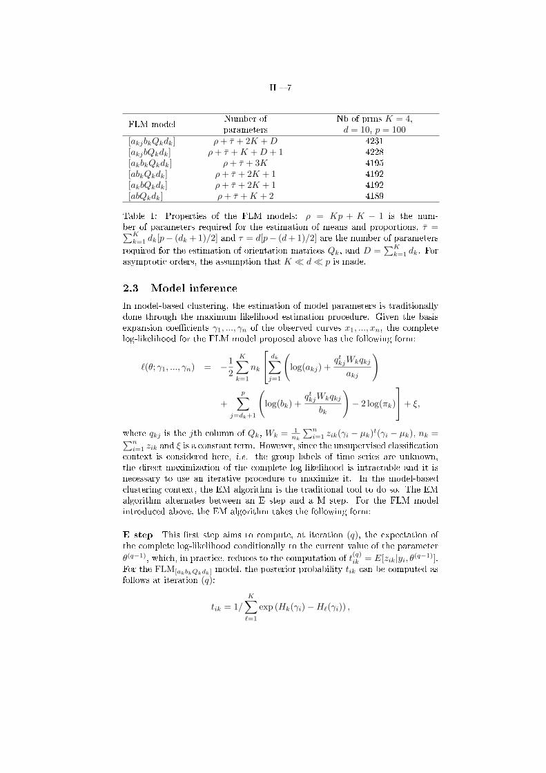
Following the strategy of [4], it is possible to obtain parsimonious submodelsfrom the FLM[akjbkQkdk] model by constraining model parameters within orbetween groups. For instance, �xing the �rst dk eigenvalues to be commonwithin each class, we obtain the more restricted model FLM[akbkQkdk]. Weobserved that the model FLM[akbkQkdk] often gives satisfying results and thissuggests that the assumption that each matrix ∆k contains only two di�erenteigenvalues, ak and bk, seems to be an e�cient way to regularize the estimationof ∆k. Another possible type of regularization is to �x the parameters bk tobe common between the classes. This yields the models FLM[akjbQkdk] andFLM[akbQkdk] which both assume that the variance outside the class speci�csubspaces is common. This assumption can be viewed as modeling the noiseoutside the latent subspace of the group by a single parameter b which is anatural hypothesis when the data are obtained in a common acquisition process.Among the 28 models proposed in the original article [4], 6 models have beenselected for their good practical behaviors to be considered in the experimentsof Section 3. Table 1 lists those 6 models and their corresponding complexity(i.e. the number of parameters to estimate).

II � 7

FLM modelNumber ofparameters

Nb of prms K = 4,d = 10, p = 100

[akjbkQkdk] ρ+ τ + 2K +D 4231[akjbQkdk] ρ+ τ +K +D + 1 4228[akbkQkdk] ρ+ τ + 3K 4195[abkQkdk] ρ+ τ + 2K + 1 4192[akbQkdk] ρ+ τ + 2K + 1 4192[abQkdk] ρ+ τ +K + 2 4189

Table 1: Properties of the FLM models: ρ = Kp + K − 1 is the num-ber of parameters required for the estimation of means and proportions, τ =∑Kk=1 dk[p− (dk + 1)/2] and τ = d[p− (d+ 1)/2] are the number of parameters

required for the estimation of orientation matrices Qk, and D =∑Kk=1 dk. For

asymptotic orders, the assumption that K � d� p is made.

2.3 Model inference

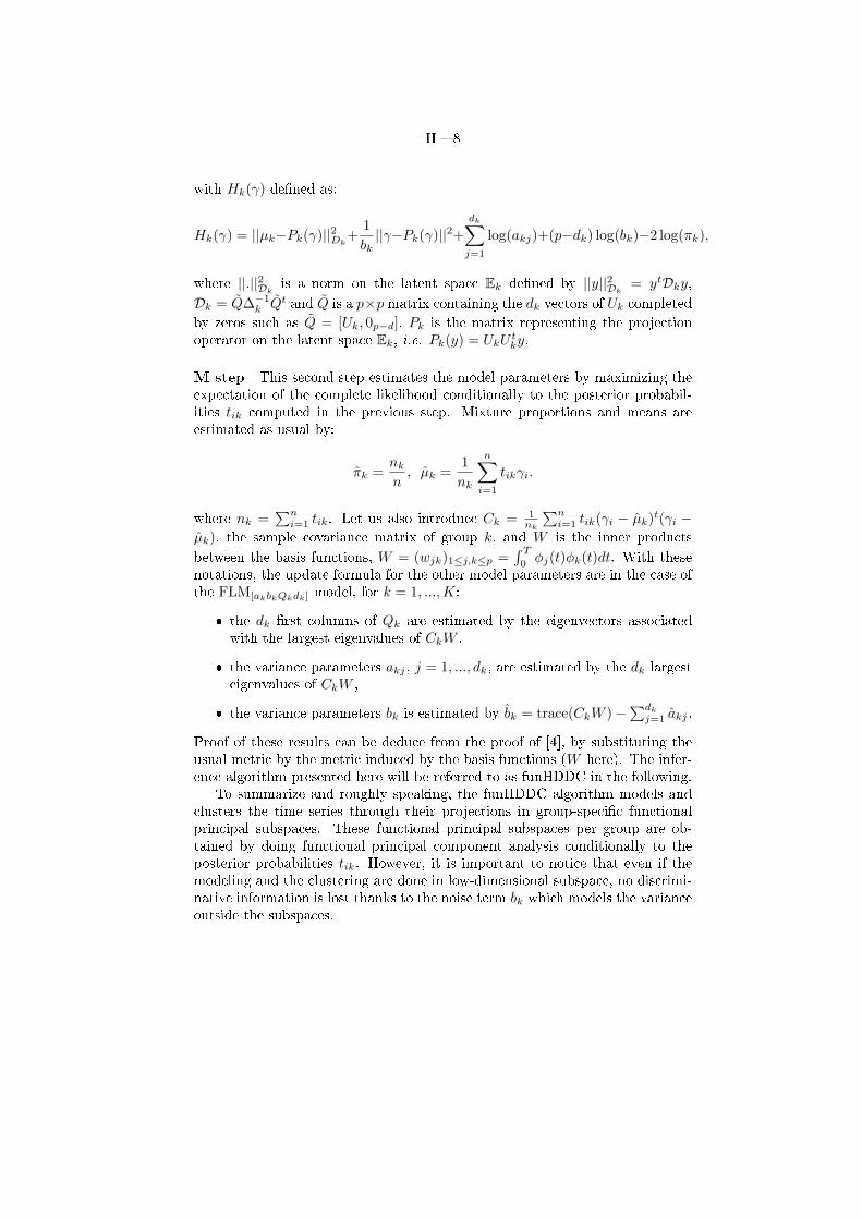
In model-based clustering, the estimation of model parameters is traditionallydone through the maximum likelihood estimation procedure. Given the basisexpansion coe�cients γ1, ..., γn of the observed curves x1, ..., xn, the completelog-likelihood for the FLM model proposed above has the following form:

`(θ; γ1, ..., γn) = −1

2

K∑k=1

nk

dk∑j=1

(log(akj) +

qtkjWkqkj

akj

)

+

p∑j=dk+1

(log(bk) +

qtkjWkqkj

bk

)− 2 log(πk)

+ ξ,

where qkj is the jth column of Qk, Wk = 1nk

∑ni=1 zik(γi − µk)t(γi − µk), nk =∑n

i=1 zik and ξ is a constant term. However, since the unsupervised classi�cationcontext is considered here, i.e. the group labels of time series are unknown,the direct maximization of the complete log-likelihood is intractable and it isnecessary to use an iterative procedure to maximize it. In the model-basedclustering context, the EM algorithm is the traditional tool to do so. The EMalgorithm alternates between an E step and a M step. For the FLM modelintroduced above, the EM algorithm takes the following form:

E step This �rst step aims to compute, at iteration (q), the expectation ofthe complete log-likelihood conditionally to the current value of the parameter

θ(q−1), which, in practice, reduces to the computation of t(q)ik = E[zik|yi, θ(q−1)].

For the FLM[akbkQkdk] model, the posterior probability tik can be computed asfollows at iteration (q):

tik = 1/

K∑`=1

exp (Hk(γi)−H`(γi)) ,

II � 8

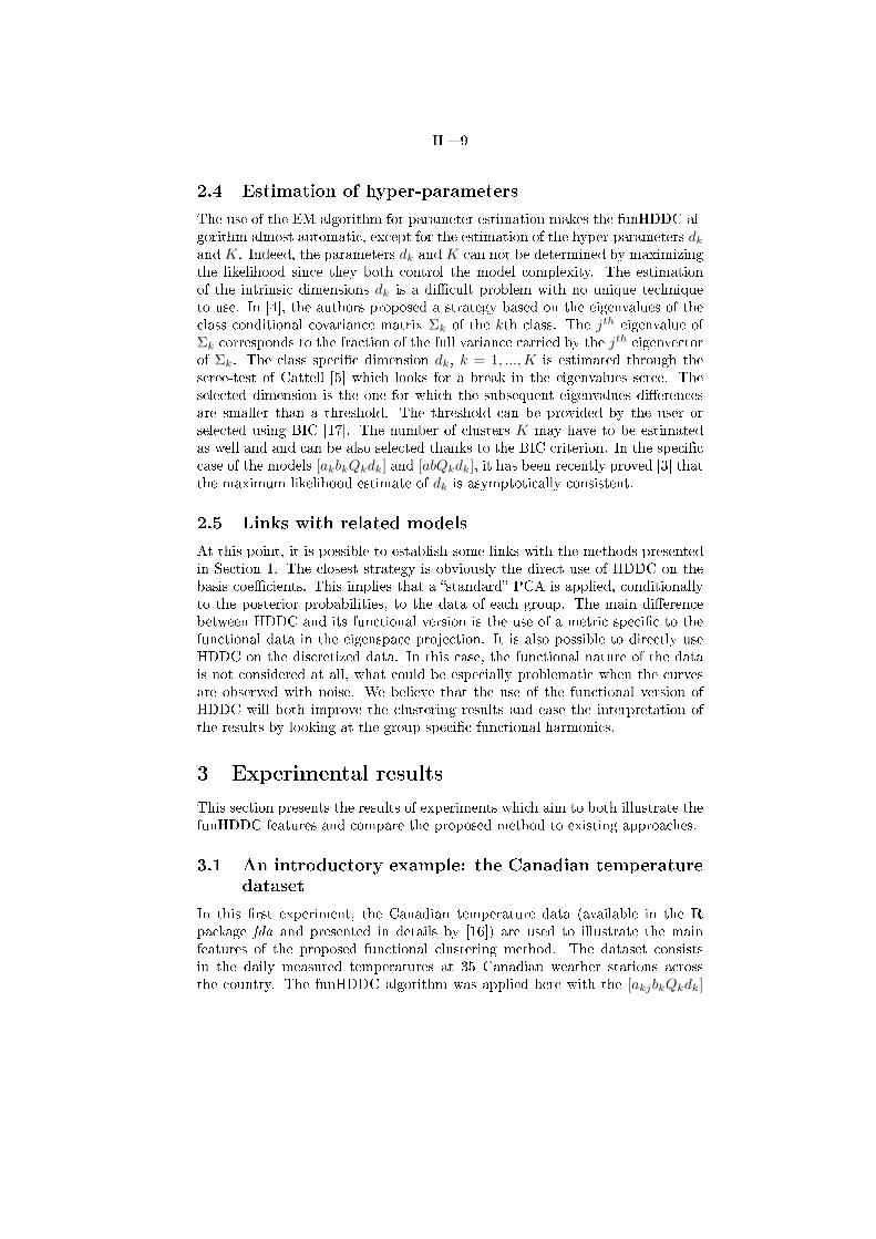
with Hk(γ) de�ned as:

Hk(γ) = ||µk−Pk(γ)||2Dk+

1

bk||γ−Pk(γ)||2+

dk∑j=1

log(akj)+(p−dk) log(bk)−2 log(πk),

where ||.||2Dkis a norm on the latent space Ek de�ned by ||y||2Dk

= ytDky,Dk = Q∆−1k Qt and Q is a p×p matrix containing the dk vectors of Uk completed

by zeros such as Q = [Uk, 0p−d], Pk is the matrix representing the projectionoperator on the latent space Ek, i.e. Pk(y) = UkU

tky.

M step This second step estimates the model parameters by maximizing theexpectation of the complete likelihood conditionally to the posterior probabil-ities tik computed in the previous step. Mixture proportions and means areestimated as usual by:

πk =nkn, µk =

1

nk

n∑i=1

tikγi.

where nk =∑ni=1 tik. Let us also introduce Ck = 1

nk

∑ni=1 tik(γi − µk)t(γi −

µk), the sample covariance matrix of group k, and W is the inner products

between the basis functions, W = (wjk)1≤j,k≤p =´ T0φj(t)φk(t)dt. With these

notations, the update formula for the other model parameters are in the case ofthe FLM[akbkQkdk] model, for k = 1, ...,K:

� the dk �rst columns of Qk are estimated by the eigenvectors associatedwith the largest eigenvalues of CkW ,

� the variance parameters akj , j = 1, ..., dk, are estimated by the dk largesteigenvalues of CkW ,

� the variance parameters bk is estimated by bk = trace(CkW )−∑dkj=1 akj .

Proof of these results can be deduce from the proof of [4], by substituting theusual metric by the metric induced by the basis functions (W here). The infer-ence algorithm presented here will be referred to as funHDDC in the following.

To summarize and roughly speaking, the funHDDC algorithm models andclusters the time series through their projections in group-speci�c functionalprincipal subspaces. These functional principal subspaces per group are ob-tained by doing functional principal component analysis conditionally to theposterior probabilities tik. However, it is important to notice that even if themodeling and the clustering are done in low-dimensional subspace, no discrimi-native information is lost thanks to the noise term bk which models the varianceoutside the subspaces.

II � 9

2.4 Estimation of hyper-parameters

The use of the EM algorithm for parameter estimation makes the funHDDC al-gorithm almost automatic, except for the estimation of the hyper-parameters dkand K. Indeed, the parameters dk and K can not be determined by maximizingthe likelihood since they both control the model complexity. The estimationof the intrinsic dimensions dk is a di�cult problem with no unique techniqueto use. In [4], the authors proposed a strategy based on the eigenvalues of theclass conditional covariance matrix Σk of the kth class. The jth eigenvalue ofΣk corresponds to the fraction of the full variance carried by the jth eigenvectorof Σk. The class speci�c dimension dk, k = 1, ...,K is estimated through thescree-test of Cattell [5] which looks for a break in the eigenvalues scree. Theselected dimension is the one for which the subsequent eigenvalues di�erencesare smaller than a threshold. The threshold can be provided by the user orselected using BIC [17]. The number of clusters K may have to be estimatedas well and and can be also selected thanks to the BIC criterion. In the speci�ccase of the models [akbkQkdk] and [abQkdk], it has been recently proved [3] thatthe maximum likelihood estimate of dk is asymptotically consistent.

2.5 Links with related models

At this point, it is possible to establish some links with the methods presentedin Section 1. The closest strategy is obviously the direct use of HDDC on thebasis coe�cients. This implies that a �standard� PCA is applied, conditionallyto the posterior probabilities, to the data of each group. The main di�erencebetween HDDC and its functional version is the use of a metric speci�c to thefunctional data in the eigenspace projection. It is also possible to directly useHDDC on the discretized data. In this case, the functional nature of the datais not considered at all, what could be especially problematic when the curvesare observed with noise. We believe that the use of the functional version ofHDDC will both improve the clustering results and ease the interpretation ofthe results by looking at the group-speci�c functional harmonics.

3 Experimental results

This section presents the results of experiments which aim to both illustrate thefunHDDC features and compare the proposed method to existing approaches.

3.1 An introductory example: the Canadian temperature

dataset

In this �rst experiment, the Canadian temperature data (available in the Rpackage fda and presented in details by [16]) are used to illustrate the mainfeatures of the proposed functional clustering method. The dataset consistsin the daily measured temperatures at 35 Canadian weather stations acrossthe country. The funHDDC algorithm was applied here with the [akjbkQkdk]

II � 10

1 2 3 4 5

−400000

−300000

−200000

−100000

Number of groups

BIC

valu

e

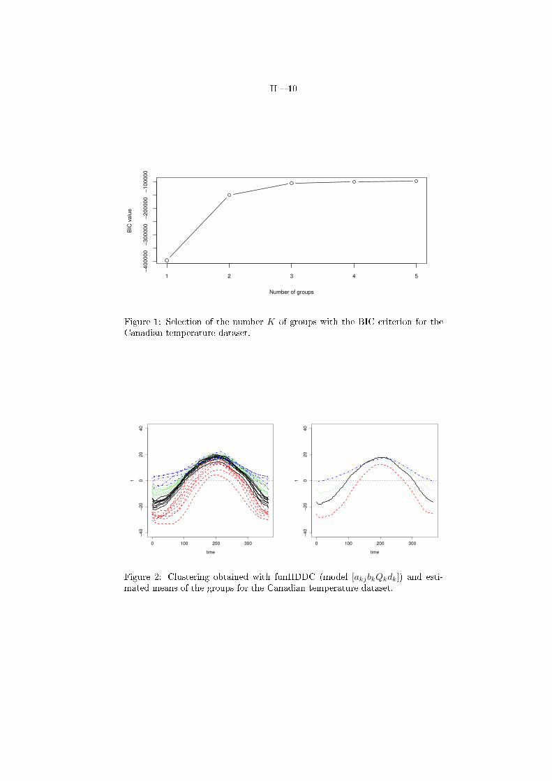
Figure 1: Selection of the number K of groups with the BIC criterion for theCanadian temperature dataset.

0 100 200 300

−4

0−

20

02

04

0

time

1

0 100 200 300

−4

0−

20

02

04

0

time

1

Figure 2: Clustering obtained with funHDDC (model [akjbkQkdk]) and esti-mated means of the groups for the Canadian temperature dataset.

II � 11

St. Johns

HalifaxSydney

YarmouthCharlottvl

Fredericton

Scheffervll

ArvidaBagottvilleQuebec

SherbrookeMontrealOttawaToronto

London

ThunderbayWinnipeg

The Pas

Churchill

Regina

Pr. Albert

Uranium Cty

Edmonton

CalgaryKamloopsVancouver

Victoria

Pr. GeorgePr. Rupert

Whitehorse

DawsonYellowknife

Iqaluit

Inuvik

Resolute

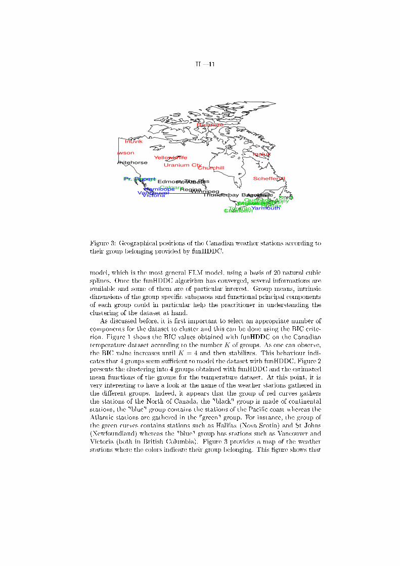
Figure 3: Geographical positions of the Canadian weather stations according totheir group belonging provided by funHDDC.

model, which is the most general FLM model, using a basis of 20 natural cubicsplines. Once the funHDDC algorithm has converged, several informations areavailable and some of them are of particular interest. Group means, intrinsicdimensions of the group-speci�c subspaces and functional principal componentsof each group could in particular help the practitioner in understanding theclustering of the dataset at hand.

As discussed before, it is �rst important to select an appropriate number ofcomponents for the dataset to cluster and this can be done using the BIC crite-rion. Figure 1 shows the BIC values obtained with funHDDC on the Canadiantemperature dataset according to the number K of groups. As one can observe,the BIC value increases until K = 4 and then stabilizes. This behaviour indi-cates that 4 groups seem su�cient to model the dataset with funHDDC. Figure 2presents the clustering into 4 groups obtained with funHDDC and the estimatedmean functions of the groups for the temperature dataset. At this point, it isvery interesting to have a look at the name of the weather stations gathered inthe di�erent groups. Indeed, it appears that the group of red curves gathersthe stations of the North of Canada, the "black" group is made of continentalstations, the "blue" group contains the stations of the Paci�c coast whereas theAtlantic stations are gathered in the "green" group. For instance, the group ofthe green curves contains stations such as Halifax (Nova Scotia) and St Johns(Newfoundland) whereas the "blue" group has stations such as Vancouver andVictoria (both in British Columbia). Figure 3 provides a map of the weatherstations where the colors indicate their group belonging. This �gure shows that

II � 12

0 100 200 300

−40

−20

020

40

time

1

0 100 200 300

−40

−20

020

40

PCA function 1 (Percentage of variability 85.1 )

Time

Harm

onic

1

++++++++++++++++

++++++++++++++++++++++++++++++++

+++++++++++

+++++++++++++++++++++++++++++++++++++++++++++++++++++++++++++++++++++

−−−−−−−−−−−−−−

−−−−−−−−

−−−−−−−−−−−−−−−−−−−−−−−−−−−−−−−−−−−−−

−−−−−−−−−−−−−−−−−−−−−−−−−−−−−−−−−−−−−−−−−−−−−−−−−−−−−−−−−−−−−−−−−−−−−

0 100 200 300

−40

−20

020

40

PCA function 2 (Percentage of variability 17.6 )

Time

Harm

onic

2

+++++++++++++++

+++++++++++++++++++++++++++++++++++++++

++++++++++++++++++++++++++++++++++++++++++++++++++++++++++++++++++++++++++

−−−−−−−−−−−−−−−−

−−−−−−−−−−−−−−−−−−−−−−−−−−−−−−−−−−−−−−−−−−−

−−−−−−−−−−−−−−−−−−−−−−−−−−−−−−−−−−−−−−−−−−−−−−−−−−−−−−−−−−−−−−−−−−−−−

(a) Continental

0 100 200 300

−40

−20

020

40

time

1

0 100 200 300

−40

−20

020

40

PCA function 1 (Percentage of variability 98.2 )

Time

Harm

onic

1

+++++++++++++++++++++

++++++++++++++++++++++++

+++++++++++++

+++++++++++

+++++++++++++++++++++++++++++++++++++++++++++++++++++++++++

−−−−−−−−−

−−−−−−−−−−−−−−−−−−−−−−−−−−−−−−−−−−−−−−−−−−−−−−−−−−−−−−−−−−−−−−−−−−−−−−−−−−−−−−−−−−−−−−−−−−−−−−−−−−−−−−−−−−−−−−−−−−−−−−−

0 100 200 300

−40

−20

020

40

PCA function 2 (Percentage of variability 2.4 )

Time

Harm

onic

2

+++++++++++++++++

+++++++++++++++++++++++++++++++++++++++++++++

++++++++++++++++++++++++++++++++++++++++++++++++++++++++++++++++++

−−−−−−−−−−−−−−−−−−−−−

−−−−−−−−−−−−−−−−−−−−−−−−−−−−−−−−−−−−−−−−−−

−−−−−−−−−−−−−−−−−−−−−−−−−−−−−−−−−−−−−−−−−−−−−−−−−−−−−−−−−−−−−−−−−

(b) Arctic

0 100 200 300

−40

−20

020

40

time

1

0 100 200 300

−40

−20

020

40

PCA function 1 (Percentage of variability 91.1 )

Time

Harm

onic

1

++++++++++++++++++++++++++++

++++++++++

++++++++++++++

+++++++++++++

+++++++++++++++++++++++++++++++++++++++++++++++++++++++++++++++

−−−−−−−−−−−−−−−−−−−

−−−−−−−−−−−−−−−−−−−−−−−−−−−−−−−−−−−−−−−−−−−

−−−−−−−−−−−−−−−−−−−−−−−−−−−−−−−−−−−−−−−−−−−−−−−−−−−−−−−−−−−−−−−−−−

0 100 200 300

−40

−20

020

40

PCA function 2 (Percentage of variability 6.5 )

Time

Harm

onic

2

+++++++++++++++++

++++++++++++++++++++++++++++++++++++++

++++++++++++

+++++++++++++++++++++++++++++++++++++++++++++++++++++++++++++−−−−−−−−−−−−−−−−−−−

−−−−−−−−−−−−−−−−

−−−−−−−−−−−

−−−−−−−−−

−−−−−−−−−

−−−−−−−−−−−−−−−−−−−−−−−−−−−−−−−−−−−−−−−−−−−−−−−−−−−−−−−−−−−−−−−−

(c) Atlantic

0 100 200 300

−40

−20

020

40

time

1

0 100 200 300

−40

−20

020

40

PCA function 1 (Percentage of variability 97.5 )

Time

Harm

onic

1

+++++++++++++++

++++++++++++++++++++++++++++++

++++++++++

++++++++++++++

+++++++++++++++++++++++++++++++++++++++++++++++++++++++++++

−−−−−−−−−−−−−−−−−−−

−−−−−−−−−−

−−−−−−−−

−−−−−−−−

−−−−−−−−−−−−

−−−−−−−−−−−−−−−−−−−−−−−−−−−−−−−−−−−−−−−−−−−−−−−−−−−−−−−−−−−−−−−−−−−−−−−

0 100 200 300

−40

−20

020

40

PCA function 2 (Percentage of variability 12.5 )

Time

Harm

onic

2

+++++++++++++++++++

++++++++

++++++++++

++++++++++

++++++++++

+++++++++++++++++++++++++++++++++++++++++++++++++++++++++++++++++++++++

−−−−−−−−−−−−−−−−−−−−−−−−

−−−−−−−−−−−−−−−−

−−−−−−−−−−−

−−−−−−−−−−−−−−−−

−−−−−−−−−−−−−−−−−−−−−−−−−−−−−−−−−−−−−−−−−−−−−−−−−−−−−−−−−−−−−

(d) Paci�c

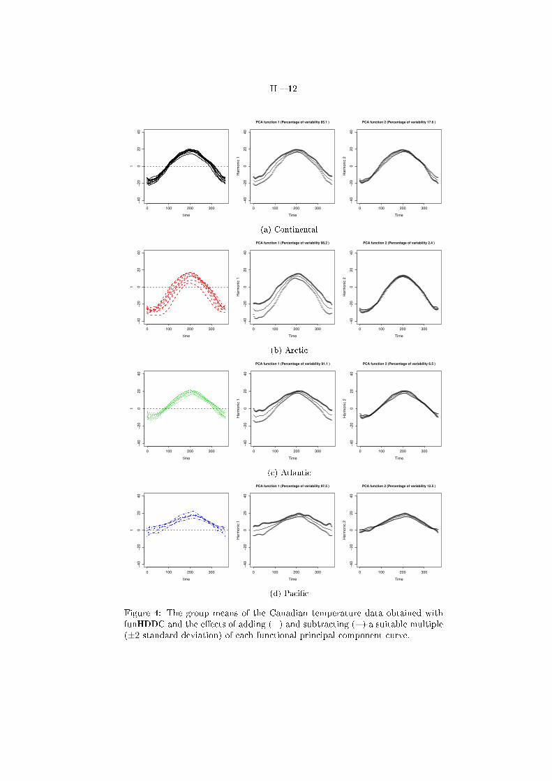
Figure 4: The group means of the Canadian temperature data obtained withfunHDDC and the e�ects of adding (+) and subtracting (=) a suitable multiple(±2 standard deviation) of each functional principal component curve.

II � 13

−300 −200 −100 0 100 200

−1

00

−5

00

50

Subspace of group 1

St. Johns

Halifax

SydneyYarmouth

Charlottvl

FrederictonScheffervll

ArvidaBagottvilleQuebec

SherbrookeMontrealOttawa

TorontoLondon

Thunder Bay

WinnipegThe Pas

Churchill

ReginaPr. Albert

Uranium City

Edmonton

CalgaryKamloops

VancouvVictoria

Pr. George

Pr. Rupert

Whitehorse

Dawson

Yellowknife

Iqaluit

Inuvik

Resolute

−100 0 100 200 300

−8

0−

60

−4

0−

20

02

04

0

Subspace of group 2

St. Johns

Halifax

SydneyYarmouth

Charlottvl

Fredericton

Scheffervll

ArvidaBagottvilleQuebec

Sherbrooke

MontrealOttawa

TorontoLondonThunder Bay

Winnipeg

The Pas

Churchill

ReginaPr. AlbertUranium City

Edmonton

Calgary

Kamloops

Vancouv

Victoria

Pr. George

Pr. Rupert

Whitehorse

DawsonYellowknife

Iqaluit

Inuvik

Resolute

−400 −300 −200 −100 0 100

−1

00

−5

00

Subspace of group 3

St. Johns

Halifax

SydneyYarmouth

Charlottvl

Fredericton

Scheffervll

ArvidaBagottvilleQuebec

Sherbrooke

MontrealOttawa

TorontoLondonThunder Bay

Winnipeg

The Pas

Churchill

ReginaPr. AlbertUranium City

Edmonton

Calgary

Kamloops

Vancouv

Victoria

Pr. George

Pr. Rupert

Whitehorse

DawsonYellowknife

Iqaluit

Inuvik

Resolute

−400 −300 −200 −100 0

−1

00

−5

00

50

Subspace of group 4

St. Johns

Halifax

SydneyYarmouth

Charlottvl

Fredericton

Scheffervll

ArvidaBagottvilleQuebec

Sherbrooke

MontrealOttawa

TorontoLondon

Thunder Bay

Winnipeg

The Pas

Churchill

ReginaPr. AlbertUranium City

Edmonton

Calgary

Kamloops

VancouvVictoria

Pr. George

Pr. Rupert

Whitehorse

DawsonYellowknife

Iqaluit

Inuvik

Resolute

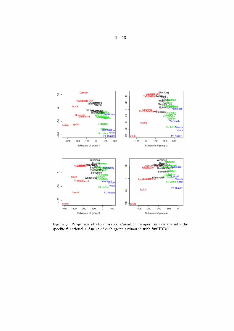
Figure 5: Projection of the observed Canadian temperature curves into thespeci�c functional subspace of each group estimated with funHDDC.

II � 14

the obtained clustering with funHDDC is very satisfying and rather coherentwith the actual geographical positions of the stations (the clustering accuracy is71% here). We recall that this partition of the data has been obtained withoutany other information than the temperature curves. In addition, the observa-tion of the temperature means of the 4 groups con�rms the common idea thatseasons are more rude in the North of Canada than in the South and that thecontinental cities have lower temperatures than coast cities during the winter.

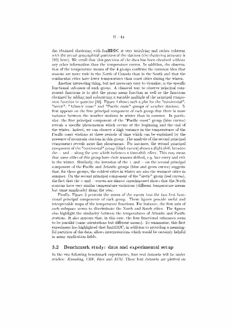
Another interesting thing, but not necessary easy to visualize, is the speci�cfunctional subspace of each group. A classical way to observe principal com-ponent functions is to plot the group mean function as well as the functionsobtained by adding and subtracting a suitable multiple of the principal compo-nent function in question [16]. Figure 4 shows such a plot for the "continental","arctic", "Atlantic coast" and "Paci�c coast" groups of weather stations. It�rst appears on the �rst principal component of each group that there is morevariance between the weather stations in winter than in summer. In partic-ular, the �rst principal component of the "Paci�c coast" group (blue curves)reveals a speci�c phenomenon which occurs at the beginning and the end ofthe winter. Indeed, we can observe a high variance in the temperatures of thePaci�c coast stations at these periods of time which can be explained by thepresence of mountain stations in this group. The analysis of the second principalcomponents reveals more �ne phenomena. For instance, the second principalcomponent of the "continental" group (black curves) shows a slight shift betweenthe + and = along the year which indicates a time-shift e�ect. This may meanthat some cities of this group have their seasons shifted, e.g. late entry and exitin the winter. Similarly, the inversion of the + and = on the second principalcomponent of the Paci�c and Atlantic groups (blue and green curves) suggeststhat, for these groups, the coldest cities in winter are also the warmest cities insummer. On the second principal component of the "arctic" group (red curves),the fact that the + and = curves are almost superimposed shows that the Northstations have very similar temperature variations (di�erent temperature meansbut same amplitude) along the year.

Finally, Figure 5 presents the scores of the curves into the two �rst func-tional principal components of each group. These �gures provide useful andinterpretable maps of the temperature functions. For instance, the �rst axis ofeach subspace seems to discriminate the North and South cities. The �guresalso highlight the similarity between the temperatures of Atlantic and Paci�cstations. It also appears that, in this case, the four functional subspaces seemto be parallel (same orientations but di�erent means). To summarize, this �rstexperiment has highlighted that funHDDC, in addition to providing a meaning-ful partition of the data, allows interpretations which would be certainly helpfulin many application �elds.

3.2 Benchmark study: data and experimental setup

In the two following benchmark experiments, four real datasets will be understudies: Kneading, CBF, Face and ECG. These four datasets are plotted on

II � 15

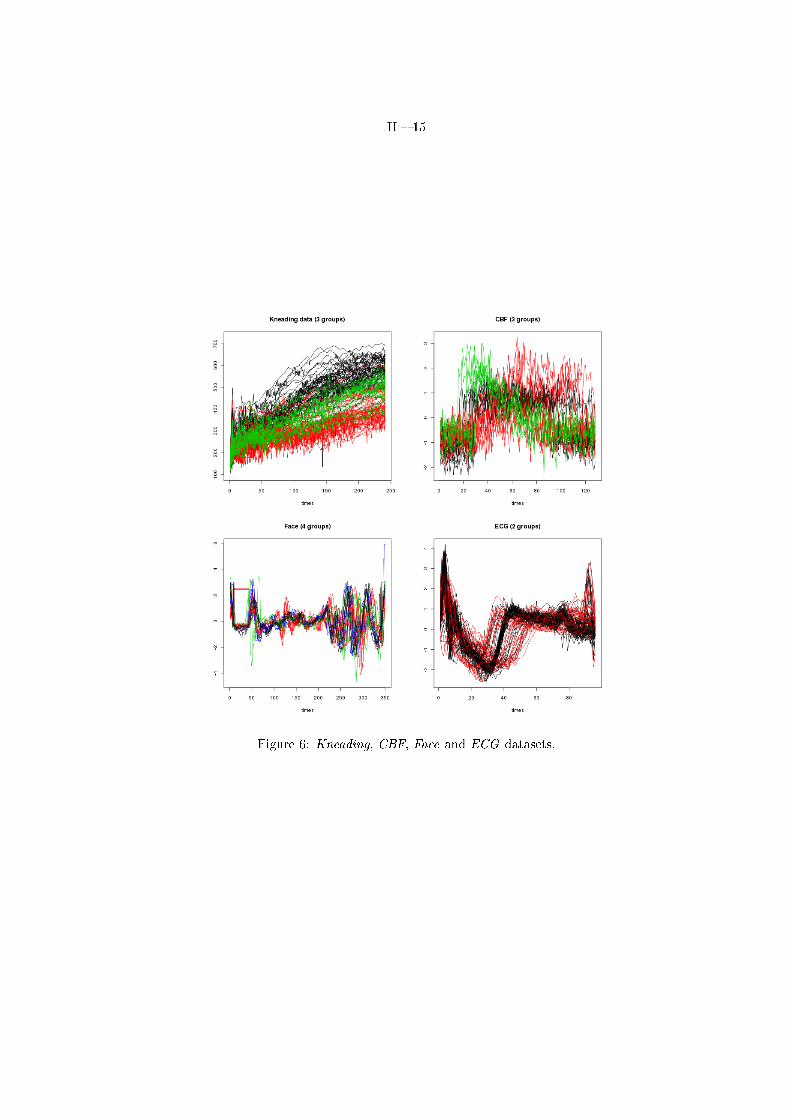
Figure 6: Kneading, CBF, Face and ECG datasets.

II � 16

Figure 6. The �rst dataset (Kneading) comes from a study which consisted inpredicting the quality of cookies (good, adjustable or bad) from the kneadingcurve representing the resistance (density) of dough observed during the knead-ing process. The corresponding dataset is made of 115 curves observed at 241equispaced instants of the time. Among the 115 cookies, 50 have been judgedgood, 25 adjustable and 40 bad. These data, provided by the Danone company,have been already studied in a supervised context [13, 15]. These data areknown to be hard to discriminate, even for supervised classi�ers, partly becauseof the adjustable class. The three other datasets come from the UCR TimeSeries Classi�cation and Clustering website1. The CBF dataset is made of 930curves sampled from 3 groups at 128 instants of time. The Face dataset [22]consists of 112 curves sampled from 4 groups at 350 instants of time. Finally,the ECG dataset [14] consists of 200 curves from 2 groups sampled at 96 timeinstants.

In the following, two benchmark experiments will allow to compare the clus-tering ability of the funHDDC method with state-of-the-art methods. First,funHDDC will be compared to the fclust method of James and Sugar, describedin Section 1, which has also the advantage to take into account the functionalnature of the data. Second, funHDDC will be compared to usual two-step meth-ods in which the functional data are �rst transformed into a �nite dimensionalvector (simple time discretization, projection into a natural cubic spline basisor onto functional principal components) and then clustered by an usual clus-tering method (HDDC [4], MixtPPCA [19], kmeans or GMM [2, 6] through theR package mclust).

3.3 Benchmark study: comparison with fclust

A package implementing fclust for the R software is available on the author'swebsite. However, because of a memory limitation in this package, we hadto select a reduced number of curves from the original four datasets. For theKneading data, 50 curves have been randomly chosen in the 115 original ones,and for the three other datasets, which are separated into a training and atest sample on the UCR website (for supervised classi�cation purpose), onlythe training part have been kept. For funHDDC, a basis of 20 natural cubicsplines has been chosen for each dataset. The clustering results are providedby Table 2 which indicates the correct classi�cation rates for both methods,the BIC values and the intrinsic dimensions for each group-speci�c functionalsubspace for funHDDC. These results clearly show that funHDDC outperformsfclust on all the datasets. Moreover, it appears that the BIC criterion, usedfor choosing the number of dimensions (tuned by a common threshold) and themost appropriate submodel, leads to often select the most e�cient funHDDCmodels (for three datasets among four). It should nevertheless be noticed thatfclust has been developed especially for sparsely sampled functional data, andit would be interesting to compare both methods on such data too.

1http://www.cs.ucr.edu/∼eamonn/time_series_data/

II � 17

dataset Kneading CBF

groups number 3 3

size 502 30

method cc BIC d cc BIC d

Fun-HDDC AkjBkQkDk 70 -2403 (2,1,1) 63.3 -2430 (1,1,1)Fun-HDDC AkjBQkDk 66.6 -2498 (1,1,1) 63.3 -2498 (1,1,1)Fun-HDDC AkBkQkDk 70 -2193 (1,1,1) 56.6 -2514 (1,1,1)Fun-HDDC AkBQkDk 66.6 -2402 (1,1,1) 63.3 -2402 (1,1,1)Fun-HDDC ABkQkDk 66.6 -2195 (1,2,1) 56.6 -2523 (1,1,1)Fun-HDDC ABQkDk 66.6 -2397 (1,1,1) 63.3 -2397 (1,1,1)

fclust3 60 56.6

dataset Face ECG

groups number 4 2

size 24 100

method cc BIC d cc BIC d

Fun-HDDC AkjBkQkDk 62.5 -2162 (1,1,2,1) 77 -6667 (1,1)Fun-HDDC AkjBQkDk 50 -2286 1,1,1,1) 76 -6428 (1,1)Fun-HDDC AkBkQkDk 62.5 -2078 (2,1,1,1) 77 -6333 (1,1)Fun-HDDC AkBQkDk 58.3 -2083 (1,2,1,1) 77 -6191 (1,1)Fun-HDDC ABkQkDk 66.6 -2092 (2,1,2,1) 77 -6317 (1,1)Fun-HDDC ABQkDk 58.3 -2080 (2,1,1,1) 77 -6167 (1,1)

fclust4 41.6 75

Table 2: Percentages of correct classi�cation (cc), BIC values (if available), anddimension of each class-speci�c functional subspace (d) for methods fclust andfunHDDC on parts of the Kneading, CBF, Face and ECG datasets.

II � 18

Fun-HDDCKneading Kneading

functional2-steps discretized spline coe�. FPCA scoresmethods (241 instants) (20 splines) (4 components)

AkjBkQkDk 64.35 HDDC 66.09 53.91 44.35AkjBQkDk 62.61 MixtPPCA 65.22 64.35 62.61AkBkQkDk 64.35 mclust 63.48 50.43 60AkBQkDk 62.61 kmeans 62.61 62.61 62.61ABkQkDk 64.35ABQkDk 62.61

Fun-HDDCCBF CBF

functional2-steps discretized spline coe�. FPCA scoresmethods (128 instants) (20 splines) (17 components)

AkjBkQkDk 64.84 HDDC 68.60 51.18 68.17AkjBQkDk 70.43 MixtPPCA 65.59 51.29 68.27AkBkQkDk 64.09 mclust 61.18 62.79 68.06AkBQkDk 70.65 kmeans 64.95 54.09 64.84ABkQkDk 70.65ABQkDk 70.65

Fun-HDDCFace Face

functional2-steps discretized spline coe�. FPCA scoresmethods (350 instants) (20 splines) (3 components)

AkjBkQkDk 56.25 HDDC 59.82 58.03 63.39AkjBQkDk 54.44 MixtPPCA 54.54 61.36 64.77

AkBkQkDk 51.78 mclust 62.5 57.14 55.36AkBQkDk 54.44 kmeans 59.09 53.41 59.09ABkQkDk 60.71ABQkDk 57.14

Fun-HDDCECG ECG

functional2-steps discretized spline coe�. FPCA scoresmethods (96 instants) (20 splines) (19 components)

AkjBkQkDk 75 HDDC 74.5 73.5 74.5AkjBQkDk - MixtPPCA 74.5 73.5 74.5AkBkQkDk 76.5 mclust 81 80.5 81.5

AkBQkDk 74.5 kmeans 74.5 72.5 74.5ABkQkDk 76.5ABQkDk 75

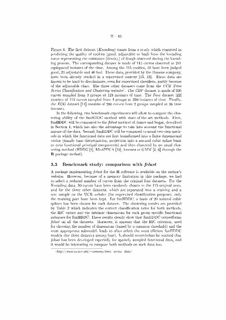
Table 3: Percentages of correct classi�cation for funHDDC (underlined for thebest model according BIC) and usual two-steps methods on the Kneading, CBF,Face and ECG datasets.

3.4 Benchmark study: comparison with usual two-step

methods

In this section, the clustering performance of funHDDC is compared to theusual two-step methods described in Section 1. The clustering results are sum-marized in Table 3. For the four datasets, the correct classi�cation rates ofeach funHDDC submodels is provided, as well as for four classical clusteringmethods: HDDC, MixtPPCA, mclust and k-means. All these two-step meth-ods are successively applied on discretized data, on the coe�cients in a naturalcubic splines basis expansion (20 splines) and on functional PCA scores. ForfunHDDC, applied also with a basis of 20 natural cubic splines, the correctclassi�cation of the best model according to BIC is underlined.

For the Kneading dataset, HDDC on discretized data appears to be the bestmethod with a correct classi�cation rate of 66.09% whereas the best funHDDCmodels leads to a rate of 64.35% and the model selected by BIC obtains 62.61%.For the CBF data, the best method is funHDDC with the model selected by BIC,

II � 19

with a correct classi�cation rate of 70.65%, whereas the best classi�cation rateof the two-step methods (still provided by HDDC on discretized data) is 68.6%.For the Face data, the best approach is MixtPPCA on the functional PCA scores(64.77% versus 60.71% for funHDDC) and mclust is the most e�cient methodon the ECG data also on the FPCA scores.

Each of the studied method, except k-means, turned out to be the bestmethod at least once over the four datasets and this benchmark study is there-fore not able to elect a clear winner. The conclusion of these experimentscould be that funHDDC is nevertheless a good alternative to two-step cluster-ing methods for the clustering of functional data. Indeed, funHDDC presentsthe advantage of always providing satisfying results in addition to not requir-ing to transform the functional data into �nite dimensional data. This is animportant point since this benchmark study has also highlighted that there areno absolute best way to discretize the functional data. Table 3 in fact showsthat each discretization has allowed at least once a two-step method to win. Inaddition, since the corresponding space in which the functions are representedare not similar, model selection criteria cannot be used to choose between suchstrategies in an unsupervised classi�cation context. From this point of view, theuse of funHDDC appears to be more tenable than two-step methods, since thefunHDDC submodel selected by BIC leads to a satisfying classi�cation rate foreach dataset.

4 Conclusion

The main objective of the present work was to adapt the HDDC clusteringmethod to functional data. The resulting algorithm, called funHDDC, modelsand clusters the high-dimensional functional data of each group in a speci�cfunctional subspace. The clustering and interpretation abilities of funHDDChave been illustrated on several real-world datasets. In particular, funHDDChas been applied to the well-known Canadian temperature dataset and it pro-vided meaningful and understandable results. The proposed method has alsobeen compared on four benchmark datasets with a recent functional cluster-ing method, fclust, and with classical two-step methods. On the one hand,funHDDC turned out to clearly outperforms its functional challenger fclust.On the other hand, funHDDC appeared to be always satisfying and more sta-ble than the two-step methods which furthermore su�er from the di�culty tochoose the discetization strategy. An extension of this work would be to adaptthe funHDDC method to multi-dimensional time series. This would be possibleby using a Gaussian model with block-diagonal covariance matrices within thegroup-speci�c functional subspaces.

Acknowledgements

The authors would like to thank Professor Cristian Preda (Université Lille 1,France) for his useful comments and the interesting discussions they have had

II � 20

with him.

References

[1] A.M. Aguilera, M. Escabiasa, C. Preda, and G. Saporta. Using basis expan-sions for estimating functional pls regression. applications with chemomet-ric data. Chemometrics and Intelligent Laboratory Systems, 104(2):289�305, 2011.

[2] J.D. Ban�eld and A.E. Raftery. Model-based gaussian and non-gaussianclustering. Biometrics, 49:803�821, 1993.

[3] C. Bouveyron, G. Celeux, and S. Girard. Intrinsic dimension estimationby maximum likelihood in probabilistic PCA. Technical Report 440372,Université Paris 1, 2010.

[4] C. Bouveyron, S. Girard, and C. Schmid. High Dimensional Data Cluster-ing. Computational Statistics and Data Analysis, 52:502�519, 2007.

[5] R. Cattell. The scree test for the number of factors. Multivariate Behav.Res., 1(2):245�276, 1966.

[6] G. Celeux and G. Govaert. Gaussian parsimonious clustering models. TheJournal of the Pattern Recognition Society, 28:781�793, 1995.

[7] A. Delaigle and P. Hall. De�ning pobability density for a distribution ofrandom functions. The Annals of Statistics, 38:1171�1193, 2010.

[8] F. Ferraty and P. Vieu. Nonparametric functional data analysis. SpringerSeries in Statistics. Springer, New York, 2006.

[9] S. Frühwirth-Schnatter and S. Kaufmann. Model-based clustering of mul-tiple time series. Journal of Business and Economic Statistics, 26:78�89,2008.

[10] J.A. Hartigan and M.A. Wong. Algorithm as 1326 : A k-means clusteringalgorithm. Applied Statistics, 28:100�108, 1978.

[11] J. Jacques, C. Bouveyron, S. Girard, O. Devos, L Duponchel, , andC. Ruckebusch. Gaussian mixture models for the classi�cation of high-dimensional vibrational spectroscopy data. Journal of Chemometrics,24:719�727, 2010.

[12] G.M. James and C.A. Sugar. Clustering for sparsely sampled functionaldata. J. Amer. Statist. Assoc., 98(462):397�408, 2003.

[13] C. Lévéder, P.A. Abraham, E. Cornillon, E. Matzner-Lober, and N. Moli-nari. Discrimination de courbes de prétrissage. In Chimiométrie 2004,pages 37�43, Paris, 2004.

II � 21

[14] R.T. Olszewski. Generalized Feature Extraction for Structural PatternRecognition in Time-Series Data. PhD thesis, Carnegie Mellon University,Pittsburgh, PA, 2001.

[15] C. Preda, G. Saporta, and C. Lévéder. PLS classi�cation of functionaldata. Comput. Statist., 22(2):223�235, 2007.

[16] J. O. Ramsay and B. W. Silverman. Functional data analysis. SpringerSeries in Statistics. Springer, New York, second edition, 2005.

[17] G. Schwarz. Estimating the dimension of a model. Ann. Statist., 6:461�464,1978.

[18] T. Tarpey and K.J. Kinateder. Clustering functional data. J. Classi�cation,20(1):93�114, 2003.

[19] M. E. Tipping and C. Bishop. Mixtures of principal component analyzers.Neural Computation, 11(2):443�482, 1999.

[20] G. Wahba. Spline models for observational data. SIAM, Philadelphia, 1990.

[21] T. Warren Liao. Clustering of time series data � a survey. Pattern Recog-nition, 38:1857�1874, 2005.

[22] X. Xi, E. Keogh, C. Shelton, L. Wei, and C.A. Ratanamahatana. Fasttime series classi�cation using numerosity reduction. In 23rd InternationalConference on Machine Learning (ICML 2006), Pittsburgh, PA, 2006.