Embed Size (px)
Citation preview

Model-based Design of Hybrid Electric Marine Propulsion
System Using Modified Low-Order Ship Hull Resistance and
Propeller Thrust Models
by
Siyang Liu
Bachelor of Engineering, University of Victoria, 2018
A Thesis Submitted in Partial Fulfillment of the Requirements for the Degree of
MASTER OF APPLIED SCIENCE
in the Department of Mechanical Engineering
©Siyang Liu, 2020
University of Victoria
All rights reserved. This dissertation may not be reproduced in whole or in part, by
photocopying or other means, without the permission of the author.

ii
Supervisory Committee
Model-based Design of Hybrid Electric Marine Propulsion
System Using Modified Low-Order Ship Hull Resistance and
Propeller Thrust Models
By
Siyang Liu
Bachelor of Engineering, University of Victoria, 2018
Supervisory Committee
Dr. Zuomin Dong, Department of Mechanical Engineering
Supervisor
Dr. Brad Buckham, Department of Mechanical Engineering
Departmental Member

iii
Abstract
Supervisory Committee
Dr. Zuomin Dong, Department of Mechanical Engineering
Supervisor
Dr. Brad Buckham, Department of Mechanical Engineering
Departmental Member
Transportation is a primary pollution source contributing to 14 percent of global greenhouse
gas emissions, and 12 percent of transportation emissions came from maritime activities.
Emissions from the ferry industry, which carries roughly 2.1 billion passengers and 250 million
vehicles annually, is a major concern for the general public due to their near-shore operations.
Compared to the rapidly advancing clean automotive propulsion, fuel efficiency and emissions
improvements for marine vessels are more urgent and beneficial due to the significantly higher
petroleum fuel consumption and heavy pollutants and the relatively slow adoption of clean
propulsion technology by the marine industry. Hybrid electric propulsion, proven to be
effective for ground vehicles, presents a promising solution for more efficient clean marine
transportation. Due to the diversified hull/propulsor design and operation cycle, the
development of a hybrid electric marine propulsion system demands model-based design and
control optimization for each unique and small batch production vessel. The integrated design
and control optimization further require accurate and computation efficient hull resistance and
propulsor thrust calculation methods that can be used to predict needed propulsion power and
gauge vessel performance, energy efficiency, and emissions. This research focuses on
improving the low-order empirical hull resistance and propulsor thrust models in the
longitudinal direction by extracting model parameters from one-pass computational fluid
dynamics (CFD) simulation and testing the acquired models in integrated design optimization
of the marine propulsion system. The model is implemented in MATLAB/Simulink and
ANSYS Aqwa and validated using operation data from BC Ferries’ ship Tachek. The modified
low-order model (M-LOM) is then used in the integrated optimizations of propulsion system
component sizes and operation control strategies for another BC Ferries’ ship, Skeena Queen.
The performance, energy efficiency, and emissions of various propulsion options, including
nature gas-mechanical and natural gas-electric benchmarks, and hybrid electric alternatives of
series hybrid, parallel hybrid, and battery/pure electric are compared to demonstrate the
benefits of the new method in completing these complex tasks and hybrid electric marine
propulsion. The research forms the foundation for further studies to achieve more accurate
propulsion demand prediction and a more comprehensive lifecycle cost assessment of clean
marine propulsion solutions.

iv
Table of Contents
Supervisory Committee ............................................................................................................. ii
Abstract .................................................................................................................................... iii
Table of Contents ...................................................................................................................... iv
List of Table ............................................................................................................................. vii
List of Figure.......................................................................................................................... viii
Acknowledgments...................................................................................................................... x
Dedication ................................................................................................................................. xi
Glossary of Acronyms and Abbreviations ............................................................................... xii
Chapter 1. Introduction .............................................................................................................. 1
1.1. General Background ....................................................................................................... 1
1.2. Research Motivation ....................................................................................................... 3
1.3. Research Objective ......................................................................................................... 4
1.4. Thesis Organization ........................................................................................................ 5
Chapter 2. Application of Hybrid Electric Propulsion on Marine Vessels – A General Review
.................................................................................................................................................... 6
2.1. Hybrid Electric Propulsion System ................................................................................. 6
2.1.1 Architectures of Hybrid Electric Propulsion System .............................................. 6
Series HEPS ........................................................................................................................ 6
Parallel HEPS ..................................................................................................................... 7
Series/Parallel HEPS .......................................................................................................... 8
2.1.2 Degree of hybridization ........................................................................................... 8
Micro Hybrid ...................................................................................................................... 8
Mild Hybrid ........................................................................................................................ 9
Medium Hybrid .................................................................................................................. 9
Full Hybrid ......................................................................................................................... 9
Plug-in Hybrid .................................................................................................................... 9
2.1.3 Operation Modes ..................................................................................................... 9
2.2. State-of-the-art Hybrid Maritime Application .............................................................. 10
2.2.1 Architecture ........................................................................................................... 10
2.2.2 Components ........................................................................................................... 11
Energy converter ............................................................................................................... 12
Energy Storage System (ESS) .......................................................................................... 13
Electric Machines ............................................................................................................. 15
Electric Power Grid .......................................................................................................... 15

v
2.2.3 Technology Trend .................................................................................................. 16
2.3. Hybrid Electric System Control .................................................................................... 17
2.3.1 Rule-Based Control ............................................................................................... 18
Deterministic Rule-Based ................................................................................................. 18
Fuzzy Rule-Based ............................................................................................................. 18
2.3.2 Optimization-Based Control .................................................................................. 18
Global Optimization ......................................................................................................... 18
Online or Real-Time Optimal Control .............................................................................. 19
2.4. Lifecycle Assessment .................................................................................................... 19
Chapter 3. Ship Power Demand Prediction Using Modified Low-Order Hull Resistance and
Propeller Thrust Models .......................................................................................................... 21
3.1. Vessel Hull Resistance Model ....................................................................................... 21
3.1.1 Total Ship Resistance ............................................................................................. 21
Water-induced Hull Resistance ......................................................................................... 22
Wind-induced Upper Decks Resistance ........................................................................... 24
3.1.2 Hull Resistance Models and Calculation Methods ................................................ 25
Hull Resistance Based on Vessel Sea Trial Data .............................................................. 26
Towing Tank Hull Resistance Prediction Method ............................................................ 26
Full-Scale CFD ................................................................................................................. 26
Reduced-Order Hull Resistance Prediction Model .......................................................... 27
Low-Order Hull Resistance Prediction Model ................................................................. 27
Generic Parametric Mathematical Model Estimation Method ......................................... 28
3.2. Vessel Propeller Efficiency and Thrust Model ............................................................. 28
3.2.1 Propeller Efficiency Model.................................................................................... 28
3.2.2 Propeller Thrust Calculation .................................................................................. 29
3.3. Modified Low-Order Model and Calculation Method (M-LOMCM) .......................... 30
3.3.1 Model Related Work .............................................................................................. 30
3.3.2 Numerical Estimation of Stability Characteristics Using CFD ............................. 32
Conventional NX CFD Package ....................................................................................... 35
FloEFD Toolbox for NX ................................................................................................... 35
Ansys Aqwa ...................................................................................................................... 36
Ansys Fluent ..................................................................................................................... 37
3.4. Modified Low Order Propeller Thrust/Torque/Speed Model ....................................... 38
3.4.1 Modified Holtrop and Mennen’s Drag Based Surging Power Deduced Model .... 38
3.4.2 Pre-calculated Propeller Efficiency ....................................................................... 39

vi
Direct Efficiency Calculation ........................................................................................... 39
Efficiency Diagram Lookup ............................................................................................. 39
Computational Fluids Dynamic Simulation ..................................................................... 41
Model Comparison ........................................................................................................... 42
3.4.3 Iterative Propeller Speed Estimation Model .......................................................... 44
3.5. Software Implementation and Model Validation .......................................................... 47
3.6. Key Improvements - Stability Data-Based Model ........................................................ 51
Chapter 4. Comparison of Different Marine Propulsion Systems ........................................... 53
4.1. Selection of a Benchmark Marine Vessel – BCFS Skeena Queen ................................ 53
4.2. Natural Gas (NG) Engine Mechanical Drive ................................................................ 56
4.3. Natural Gas Engine Electric Drive ............................................................................... 58
4.4. Pure Electric Drive ........................................................................................................ 59
4.5. NG Engine Hybrid Electric Drive ................................................................................. 60
4.5.1 Series Hybrid Electric Drive .................................................................................. 60
4.5.2 Parallel Hybrid Electric Drive ............................................................................... 60
4.6. Benchmark Performance Comparison .......................................................................... 61
Chapter 5. Application to Integrated Hybrid Electric Ship Design ......................................... 64
5.1. Propulsion Power Prediction......................................................................................... 64
5.2. Hybrid Electric Propulsion System Design .................................................................. 68
5.3. Operation Control of the Hybrid Electric Vessel .......................................................... 69
5.3.1 Rule-based Stateflow Control ................................................................................ 69
5.3.2 Dynamic Programming (DP) ................................................................................. 73
5.4. Integrated Propulsion System Design and Control Optimization ................................. 77
Chapter 6. Conclusion and Future Works ................................................................................ 89
6.1. Summary ....................................................................................................................... 89
6.2. Conclusions ................................................................................................................... 90
6.3. Research Contributions ................................................................................................. 91
6.4. Future work ................................................................................................................... 92
Reference ................................................................................................................................. 94
Appendix A Coefficients for Holtrop’s method of resistance calculation ............................. 102
Appendix B Coefficients for wind resistance calculation ...................................................... 104
Appendix C Coefficients for propeller efficiency calculation ............................................... 105

vii
List of Table
Table 1: Comparison of the critical characteristics between serirs and parallel hybrid electric
architectures ............................................................................................................................. 11
Table 2: Propeller efficiency lookup table for function implementation ................................. 40
Table 3: BCFS MV Skeena Queen design details [108] .......................................................... 54
Table 4: Optimized benchmark model result comparison. ...................................................... 62
Table 5: Detailed results comparison of two different dynamic programming strategies ....... 76
Table 6: Simulation results of two nested optimizations using fixed ICE power output strategy
and variant ICE power generation .......................................................................................... 81

viii
List of Figure
Figure 1: Series hybrid electric architecture on ship ................................................................. 7
Figure 2: Parallel hybrid electric architecture on ships or vehicles ........................................... 7
Figure 3: Series-parallel hybrid electric architecture on ships ................................................... 8
Figure 4: Complex integration of series-parallel hybrid electric architecture for ship application
.................................................................................................................................................. 11
Figure 5: Summary of available control strategies [32] ........................................................... 17
Figure 6: Types of resistance experienced by ships during sailing .......................................... 22
Figure 7: Typical hull resistance estimation methods .............................................................. 26
Figure 8: Efficiency diagram of Wageningen B-Series propeller with four blades AE/AO =
0.45[104]. ................................................................................................................................. 29
Figure 9: Comparison between the dedicated ship drag regression and numerical results [102]
.................................................................................................................................................. 31
Figure 10: Rough CAD model for Tachek upper decks........................................................... 33
Figure 11: NX CAD model measurement report ..................................................................... 33
Figure 12: Measure the corresponding volume for determining draft ..................................... 34
Figure 13: Ansys Aqwa hydrodynamic diffraction set up ....................................................... 34
Figure 14: Ansys hydrostatic position results report................................................................ 34
Figure 15: Conventional build-in NX CFD solver setup ......................................................... 35
Figure 16: FloEFD NX version simulation setup and results .................................................. 36
Figure 17: Ansys Aqwa simulation setup................................................................................. 37
Figure 18: Ansys Fluent setup and results ............................................................................... 37
Figure 19: Tachek propeller efficiency based on the efficiency diagram ................................ 40
Figure 20: Propeller CFX simulation set up and results .......................................................... 41
Figure 21: Results of three tested propeller efficiency calculation methods ........................... 42
Figure 22: Power results using fixed and real RPM. ............................................................... 43
Figure 23: Tachek propeller thrust and torque coefficient ....................................................... 45
Figure 24: Comparison between measured shaft speed to the predicted shaft speed using the
backpropagation method. ......................................................................................................... 46
Figure 25: Processes flow for the subfunction contains resistance and efficiency calculation48
Figure 26: Predefined functions for setting up propeller efficiency lookup table and stability
data calculation ........................................................................................................................ 48
Figure 27: Main LOM function flow ....................................................................................... 49
Figure 28: Results comparison between predicted and actual measured shaft power profile. 50
Figure 29: Hull resistance models comparison visualization. ................................................. 51
Figure 30: A simple representation of the low-order model .................................................... 52
Figure 31: BCFS MV Skeena Queen [108] ............................................................................. 53
Figure 32: Integrated propulsion system design processes using low-order model ................ 55
Figure 33: Benchmark model for the NG-mechanical drive propulsion system ..................... 57
Figure 34: The low-order model block representation ............................................................ 57
Figure 35: Benchmark model for the NG-electric drive propulsion system ............................ 58
Figure 36: NG generator block representation......................................................................... 59
ix
Figure 37: Benchmark model for the pure battery-electric drive propulsion system .............. 59
Figure 38: Benchmark model for the series hybrid electric drive propulsion system ............. 60
Figure 39: Benchmark model for the parallel electric drive propulsion system ...................... 61
Figure 40: SKQ propeller parameter computation setup using Ansys CFX ............................ 65
Figure 41: SKQ propeller efficiency results from Aqwa CFD simulation. ............................. 65
Figure 42: SKQ propeller parameter results from Aqwa CFD simulation. ............................. 66
Figure 43: SKQ acceleration results in comparison. ............................................................... 67
Figure 44: Fully integrated series-parallel hybrid-electric propulsion system design layout for
SKQ.......................................................................................................................................... 68
Figure 45: Rule-based control scheme for SKQ series-parallel system. ................................. 70
Figure 46: Engine operation curve. .......................................................................................... 71
Figure 47: Simulation result for series-parallel configured SKQ using rule-based control. ... 72
Figure 48: Comparison between simulation results and recorded results................................ 73
Figure 49: Dynamic programming processes demonstration .................................................. 74
Figure 50: ICE power production comparison between two DP strategies ............................. 76
Figure 51: NG generator power generation comparison between two DP strategies .............. 76
Figure 52: Battery SOC comparison between two DP strategies ............................................ 77
Figure 53: Comparison between simulated power output and recorded power demand for both
control strategies. ..................................................................................................................... 77
Figure 54: Flowchart demonstration of nested two-layer optimization. .................................. 79
Figure 55: NG generator power production for two different control strategies. .................... 82
Figure 56: NG generator power profile filtrated using a 60-second moving average filter. .... 82
Figure 57: Battery SOC profile comparison between control strategies. ................................ 83
Figure 58: Comparison between simulated ship velocity and the VDR recorded velocity data.
.................................................................................................................................................. 84
Figure 59: Improved simulated ship speed comparing to the recorded ship speed. ................ 85
Figure 60: Ship “helmsman” speed PID controller implementation ....................................... 86
Figure 61: Speed controller module regulated ship speed in comparison to recorded ship speed.
.................................................................................................................................................. 87
Figure 62: Predicted shaft power, torque, and speed demand after PID controller
implementation. ....................................................................................................................... 88

x
Acknowledgments
I would like to thank my supervisor, Dr. Zuomin Dong, whose continuous support, guidance,
and feedbacks were essential in completing this research work. His expertise greatly inspired
me for this research work, and will continuously do in my future work. I would also like to
acknowledge the valuable inputs from my research mates: Li Lily Chen, Haijia Alex Zhu,
Michael Grant, and Mostafa Rahimpour. Their works are the foundations of this extended
research.

xi
Dedication
I would like to dedicate this thesis to my family members who have supported me during the
past many years. Especially for my parents, without their encouragement and good faith, I
would not be able to complete this work in a place far from home.

xii
Glossary of Acronyms and Abbreviations
AC Alternate current
BCFS BC Ferries
CAD Computer-aided design
CD Charge depleting
CFD Computation fluids dynamic
CS Charge sustaining
DC Direct current
DE Diesel-electric
DG Diesel generator
DOE Department of energy
DP Dynamic programming
EFCM Equivalent fuel consumption method
EMS Energy management system
ESS Electric storage system
EV Electric vehicle
FC Fuel cell
FCHS Fuel cell hybrid system
GHG Greenhouse gas
GPS Global positioning system
HC Hydrocarbon
HEPS Hybrid electric propulsion system
HEV Hybrid electric vehicle
HIL Hardware in loop
ICE Internal combustion engine
IMO International maritime organization
ITTC International towing tank conference
LCC Lifecycle cost
LCCA Lifecycle cost assessment
LNG Liquified natural gas
LOM Low-order model

xiii
MAPE Mean absolute percentage error
MCFC Molten carbonate fuel cell
M-LOM Modified low-order model
MPC Model predictive control
MSSR Multi-start space reducing
NG Natural gas
PEMFC Proton exchange membrane fuel cell
PHE Parallel hybrid electric
PHEPS Parallel hybrid electric propulsion system
PM Particle matters
RANS Reynolds Averaged Navier Stokes
RNG Renewable natural gas
ROM Reduced-order model
RPM Rotation per minute
SHE Series hybrid electric
SHEPS Series hybrid electric propulsion system
SOC State of charge
SOFC Solid oxide fuel cell
SPHEPS Series-parallel hybrid electric propulsion system
VDR Voyage data record

1
Chapter 1. Introduction
1.1. General Background
With the increasing world population and growing economic activities, transportation is a
primary pollution source contributing to 14 percent of global greenhouse gas emissions [1].
With increasing environmental concerns, using clean transportation technologies to achieve
decarbonization has become the priority. Among the transportation sector, ground vehicles
contributed most of the emissions and attracted most of the research efforts and investments.
Maritime activities, which contribute to about 12 percent [2] of the transportation emissions,
have fallen behind in adopting clean propulsion technologies. At present, more than 90 percent
of world trade is carried by ships [3]. On the other hand, the ferry industry alone has a similar
size to the commercial airline industry. The world ferry industry carries roughly 2.1 billion
passengers and 250 million vehicles annually [4], even without considering countries with a
vast population like China. As the largest North American ferry operator, BC Ferries (BCFS)
transport 21 million passengers and 8 million vehicles in 2019 [5]. As reported by multiple
institutes, such as the International Maritime Organization (IMO), 4.5 percent of global 𝐶𝑂2
emissions are produced by ships [6]–[8]. This amount, if left untreated, will increase by 25
percent in 2050 [8]. Compared to the rapidly advancing clean automotive propulsion, fuel
efficiency and emission improvements for marine vessels are more urgent and beneficial due
to the significantly higher petroleum fuel consumption and heavy pollutants and the relatively
slow adoption of clean propulsion technology by the marine industry. The maritime industry
sector is smaller than other transportation segments, but investment in clean transportation for
marine vessels is more effective than in the automotive industry [9].
The inherent reason for maritime pollutions is the usage of large-scale diesel engines. With
operation cost as the primary consideration, the conventional diesel engine is the first choice
for marine vessel propulsion and power generation [7]. Much research has been carried out on
sustainable maritime transports. Since the inherent pollution source is fossil fuels, cleaner
alternative energy is a generic area of interest. One of the most adopted alternatives is liquefied
natural gas (LNG), followed by renewable electricity, biodiesel, methanol, hydrogen, and even
nuclear. Those fuels have no or low carbon, sulphur, and nitrogen content, which can drastically
reduce the exhausts' pollutive contents [10]–[17].
On the other hand, researchers also focus on advanced propulsion technologies for energy
efficiency and emission improvements. Using gas turbines to replace diesel engines or
switching to auxiliary power units during docking can improve fuel efficiency [18]–[21].
Hybrid electric propulsion systems (HEPS), with optimally controlled mechanical and electric
power flow, allow the engines to operate more efficiently and supporting prolonged heavy-duty
operations, which have become a promising solution. The new and cleaner propulsion
technology may take over maritime propulsion soon. With cleaner fuels and improved engine
technologies, hybrid electric marine propulsion would resolve a large portion of the outstanding
marine emission issue.
Geertsma et al. [18] performed a detailed review of different hybrid propulsion systems with

2
corresponding control strategies. That study showed that the hybrid system benefits a ship that
sails at 40 percent or below its top speed for most of the mission. Meanwhile, if the power
demand is well spread across the mission cycle, a hybrid electric propulsion system tends to
perform better. The review also suggested that a DC power bus can considerably reduce energy
conversion losses and boost performance. Optimization of the power control strategy and
energy management system can significantly improve the performance of a HEPS. Molloy et
al. [22] detailed the potential of applying hybrid electric or pure electric technology onto small
marine vessels and thoroughly investigated HEPS's benefits and drawbacks from the overall
concept to specific components and potential market. Researchers also suggested that hybrid
electric marine propulsion technology can only be successfully developed through
collaboration between ship designers, builders, and researchers. Only then, can technology
become mature and accepted by customers. Menanan et al. [23] reviewed the HEPS
applications on small ships. Researchers argue that the hybrid system is suitable for
applications that have stochastic conditions. Different propulsion systems, depending on the
applications, require different configurations. This review concludes that hybrid-electric
propulsion is capable of minimizing fuel consumption, especially for ships that need a high
degree of freedom during maneuvering. Other researches [24]–[26] also assess the applications
of different hybrid alternatives on ships' applications.
The propulsion systems of ground vehicles and marine vessels are comparable due to many
similar elements, such as electric drive, battery energy storage system (ESS), fuel cell
powerplant, power control, and energy management strategies, and layout of the hybrid electric
powertrain. Maturing hybrid electric technologies can be applied with some modifications.
However, several challenges prevent the quick adoption of clean transportation technology.
The demand for propulsion can be accurately predicted for vehicular applications based upon
widely accepted driving cycles and established vehicle dynamics models. The performance,
energy efficiency, and emissions of different propulsion systems can be obtained using model-
based simulation tools. On the other hand, the needed propulsion power for marine vessels
cannot be quickly and accurately calculated due to the following two reasons:
Most large marine vessels are different with distinct and diversified hull geometry,
propulsor design, and operating environments. The hydrodynamics based, accurate hull
drag and propulsor thrust prediction methods require computation-intensive full-scale
computational fluids dynamic (CFD) simulations, either in direct numerical/simulation
studies [27] or for obtaining the parameters for the reduced-order hull drag and
propulsor thrust prediction models [28]. The traditional low order empirical equations
for hull drag and propulsor thrust calculations are inaccurate and not reliable [29].
Depends on their missions, the operation profile of marine vessels varies significantly
[28], including travelling velocity, sailing route, cargo load, and marine weather
conditions.
These factors determine that no standard propulsion system design and operation controls can
be representative enough. In addition, the propulsion systems for large marine vessels require
massive investment, have long operation life, and small batch production without prototype
testing and design revision opportunity. Using model based design (MBD) technology to

3
identify the optimized propulsion system design and associated control strategies for a specific
marine application becomes essential, especially for the complex hybrid electric propulsion
system with various possible design and control solutions. Integrated propulsion system design
and optimization using multiphysics simulations and hardware in the loop (HIL) testings,
introduced in hybrid electric vehicle research, are not yet available for the optimal design of
hybrid electric marine vessels. These advanced techniques need to be developed urgently to
pave the road for clean marine propulsion.
1.2. Research Motivation
This research's primary motivation is to address the previously stated issues in generating
optimal design and control solutions through MBD for hybrid electric marine vessels. A new
method for obtaining the low-order vessel hull resistance, propulsor thrust, and propulsion
power with balanced modelling accuracy and computation intensity are to be introduced and
validated using a ferry ship's acquired operation data. The method will be integrated with the
hybrid electric powertrain design and control optimization tools and implemented using the
same MATLAB/Simulink platform. The newly introduced methods and integrated modelling
tool will be applied to compare various marine propulsion options of another benchmark vessel.
The tests are used to verify the new approach’s capability for identifying the best clean, hybrid
electric propulsion solution with optimal energy efficiency and emission improvements.
Traditionally, ship design is dominated by diesel-mechanical drives. Several reasons make such
a selection an “obvious” choice. Low-cost diesel fuel has a large energy density. The diesel
engine has a high torque capability, and the mechanical propulsion system is the most
inexpensive drivetrain installed on ships. Modern, clean propulsion technologies require high
investment costs for additional generators, electric propulsion motors, high power AC or DC
power bus, battery ESS, hydrogen fuel cells, etc. The high initial costs of adopting these new
technologies and the inability to accurately predict the fuel and operation cost savings hold
back the progress of clean marine propulsion technology. Moreover, after decades of
development, diesel engine technologies are mature. When running in the peak efficiency zone,
the engine and propulsion system efficiency is comparable to other technologies. However, the
fuel efficiency and emissions of a diesel engine are heavily influenced by the vessels’
propulsion power demand. This power demand changes dramatically for fully loaded, partially
loaded, or empty ships and under unpredictable marine weather conditions with varying wind,
wave, current, and tide. Since the engine’s most efficient operation zone is only associated with
a limited range of speed and torque, the diesel-mechanical propulsion system of a near-shore
vessel only operates at its peak efficiency for a fraction of time.
A hybrid electric marine propulsion system with a combination of mechanical power flow from
the diesel engine and electric power flow from the electric ESS, generator, and propulsion
motor can overcome the stated drawbacks of traditional diesel-mechanical and diesel-electric
drives. The series hybrid electric marine propulsion system simply adds the electric ESS and
hybrid electric powertrain control to the diesel-electric propulsion system. This new design
allows the diesel generator to operate continuously at its peak energy efficiency operation zone,
leading to improved fuel efficiency and reduced emissions and fuel cost. The variant propulsion

4
power demand from the vessel operation is met by charging or drawing electric power from
the onboard battery ESS through optimal power control and energy management from the
added hybrid propulsion system control. The parallel and series/parallel hybrid electric marine
propulsion system further improves the system's energy efficiency and reduces power loss by
avoiding unnecessary energy conversations in the hybrid electric powertrain under advanced
controls. The hybrid electric marine propulsion system better utilizes the existing diesel and
natural gas (NG) fueling infrastructure. Meanwhile, high fuel energy density, low engine cost,
and long operation life are benefits of the HEPS but are often obstacles of pure electric and
hydrogen fuel cell electric vessels.
In this research, the new modified low-order Holtrop and Mennen’s (H&M) hull resistance
regression model and H&M drag and vessel surging power deduced model (two models in
combined is known as M-LOM) are first validated using the real-world vessel operation data
acquired from the BC Ferries ship Tachek [30]. Integrated marine propulsion system modelling,
design, and control optimization are then conducted based on the BC Ferries ship Skeena
Queen (SKQ). The ship’s present diesel-mechanical propulsion system is used as the
performance, energy efficiency, and emission benchmark. Using the newly introduced
modelling and simulation tools, advanced clean marine propulsion system design and control
solutions are studied.
1.3. Research Objective
As previously mentioned, the hybrid system is influenced by the ship power profile, and such
power profiles are hard to predict under certain situations. Meanwhile, based on the power
profile and sailing conditions, the hybrid system performance is not guaranteed better than
other conventional systems. To solve the difficulties and concerns, the research objective of
this study include:
Develop a capable and accurate ship propulsion power profile prediction method based
on the low-order hull resistance and propulsor thrust models, using available vessel
operation data and one-pass CFD simulations on a PC workstation;
Validate the new M-LOM using real vessel operation data;
Test the new M-LOM model though the modelling, simulations, and performance
studies on a benchmark ferry for further improvement;
Apply the newly introduced modelling method and tools in the integrated modelling
and design and control optimizations of an advanced hybrid electric propulsion system
for the testbench ferry ship to carry out the further development of the new technique.
The ultimate goal of this research is to make the integrated modelling, design, and control
optimization of the hybrid electric marine propulsion system a more practical clean vessel
design tool without the burden of sea trial and computation-intensive full-scale CFD
simulations requiring the use of a supercomputer.

5
1.4. Thesis Organization
The thesis is organized as:
Chapter 2 reviews hybrid electric propulsion technology in general and its application on ships.
The review studies the hybrid configurations, operation modes, state-of-art components and
system design, controls, and lifecycle assessment. The review aims at studying the feasibility
of hybrid-electric propulsion technology on ships.
Chapter 3 presents the development of the M-LOM, a low-order hull resistance and propeller
thrust model for ships’ power profile prediction using speed, hull geometry data, and vessel
stability data, in detail. The goal of this study is to establish a modulized Simulink model for
power prediction that can be integrated into the overall designed system.
Chapter 4 focuses on modelling the benchmark and advanced marine propulsion systems,
including natural gas-mechanical drive, natural gas-electric drive, series hybrid, parallel hybrid,
and pure electric drive. To compare the energy efficiency of these systems, this work optimizes
the system and converts all system consumptions to equivalent fuel consumptions for total
costs measurement.
Chapter 5 introduces a fully integrated model-based hybrid electric ship design using the M-
LOM and a representative benchmark ferry ship. To simultaneously optimize the component
sizes and control strategies of the hybrid electric propulsion system, a nested two-layer
optimization problem is formulated and solved using dynamic programming (DP) and the
multi-start space reducing (MSSR) global optimization algorithm. In addition, the research
considers electric energy equivalent fuel consumption and battery degradation penalty. System
optimization is based on balanced fuel consumption and battery life loss.
Chapter 6 summarizes the work, draws conclusions, and outlines the steps for future
developments.
6
Chapter 2. Application of Hybrid Electric Propulsion on
Marine Vessels – A General Review
A hybrid electric propulsion system (HEPS) is a maturing technology for improving fuel
efficiency and reduce emissions of ground vehicles. This technology also presents great
potential for various marine applications. On the other hand, the enabling model based design
(MBD) tools for developing the HEPS of various marine vessels are still not available due to
the more complex and much diversified marine applications. To better understand the key
requirements of developing the MBD tools for marine applications, this chapter presents a
review of the system architecture, key components, and control methods of HEPS and uses the
understanding to select the appropriate HEPS design for the targeted marine vessel, including
the series-parallel hybrid electric drive with natural gas (NG) engines, electric motors, DC
power bus, li-ion batteries, and system design and control optimizations.
2.1. Hybrid Electric Propulsion System
As suggested by its name, HEPS combines at least two energy sources to provide propulsion
power jointly. Conventional HEPSs utilize internal combustion engines (ICE) and battery
energy storage systems (ESS) to boost efficiency by distributing the energy based on the
external working condition and internal system device properties. Depending on the energy
distribution methods, the HEPS can be categorized into three major groups: series, parallel,
and series-parallel. Meanwhile, based on the degree of hybridization, HEPSs are grouped into
micro, mild, medium, full, and plug-in hybrid.
In this section, the ICE and battery are considered as the default energy converter and energy
storage system to illustrate the system configuration. These two devices are the most commonly
used energy sources for the HEPS; other devices such as fuel cells or flywheels are reviewed
in the later section but not demonstrate here.
2.1.1 Architectures of Hybrid Electric Propulsion System
Series HEPS
The principal characteristic of series-configured HEPSs (SHEPS) is, there is no direct
mechanical link between ICE and the final drive. The ICE is coupled with a generator for
electricity generation. Together with the ESS, two energy sources power the electric motor(s)
to propel the final drive (wheels for vehicle and propellers for vessel). ICEs suffer from low
efficiency in the low-speed region. For vehicles in urban driving conditions or vessels under
variant loading conditions, the overall system efficiency will be low since the engine frequently
enters the low-efficiency zone. SHEPS resolves the problem by allowing ICE to work in a high-
efficiency zone for electricity generation. The battery will charge or discharge depending on
the working conditions and the level of charge (also known as the state of charge). Figure 1
shows the typical series hybrid electric propulsion system architecture.

7
Figure 1: Series hybrid electric architecture on ship
The engine can potentially be downsized in SHEPS since it is mainly responsible for
maintaining the battery’s level of charge. During a mission, ICE idles or shuts down when the
battery state of charge (SOC) is high. When battery SOC is low, ICE will operate at a high-
efficiency zone for electricity generation to charge the battery or provide propulsion power. On
vehicle applications, SHEPS is suitable for urban driving conditions where the vehicle stops
frequently. For maritime applications, SHEPS offers an excellent range extension ability for
long-distance sailing.
Parallel HEPS
Parallel HEPSs (PHEPS) keep the mechanical link between the ICE and final drives and allow
mechanical power flows through the gearbox. Meanwhile, the additional ESS and electric
motor provide assistive power to the final drive to enhance the propulsion performance. Figure
2 shows the parallel drivetrain architecture [31].
Figure 2: Parallel hybrid electric architecture on ships or vehicles
For PHEPS, ICE and electric motor are on for the entire operation duration. In this case, the
control strategy can be more complex to determine power distributions and match the speed
and torque requirements. The ICE and motor need to be synchronized in output speed since
two devices jointly power the final drive. However, the parallel configuration is more compact
than SHEPS, which requires fewer energy converters and hence will have fewer conversion
losses. PHEPS is a better suit for rural driving conditions for the vehicle since speed can be
well maintained at a constant level. At a consistent power level, an ICE will have high
efficiency, and direct mechanical links enhance efficiency since no energy formation

8
conversion is required. Ferries that have pronounced cruising phases are a good fit for PHEPS
with a similar reason to ground vehicles.
Series/Parallel HEPS
The series/parallel or power-split HEPS is a unique hybrid propulsion architecture that supports
both series and parallel hybrid electric propulsion. This advanced design allows the propulsion
system to operate as a conventional ICE drive, pure electric drive, PHEPS, SHEPS, or series-
parallel HEPS (SPHEPS). A few designs achieve alternative modes by splitting the drivetrain
into sub-systems (front and rear axis) and simultaneously applying different configurations. In
contrast, others use internal connectors such as clutch, planetary gear, and electric convertor to
achieve multiple drive modes. Figure 3 shows the general configuration of the series-parallel
structure.
Figure 3: Series-parallel hybrid electric architecture on ships
Power-split HEPS is one of the most advanced HEPS designs with the most considerable
potential for fuel consumption reduction. However, since many modes are to be switched under
different conditions, the control scheme can be complex to optimize and implement.
Meanwhile, a vast amount of simulations need to be done to achieve smooth transitions
between various modes.
2.1.2 Degree of hybridization
The degree of hybridization measures the percentage of involvement of the additional energy
sources. For ground vehicles, the degree can be tiered up as micro, mild, medium, full, and
plugin hybrid [31]–[35]. However, due to the large power demand for vessels and ships, a full
hybrid with an optional plugin functionality is commonly used. The smaller degree of
hybridization is not generally considered in marine applications.
Micro Hybrid
Micro hybrid is the minimum amount of hybridization that can be achieved in a vehicle, which
only ranges from 3 to 5 kW [32][35]. Micro hybrid aims at harvesting energy from regenerative
braking for battery charging. Combined with an engine stop-start system, this hybrid system
can typically reduce up to 4 percent of the 𝐶𝑂2 emissions [32].

9
Mild Hybrid
Mild hybrid is the next tire, which typically rates at 7 to 12 kW of hybridization. A
motor/generator can harvest energy from regenerative braking, and the system benefits from
engine stop-start. Meanwhile, the motor provides assistive power during some driving
conditions. However, the battery and motor are not big enough for electric drive mode [31]–
[34].
Medium Hybrid
Medium hybrid is also known as a motor assistive hybrid. For medium hybrid, the primary
energy is the ICE, and ESS provides assistive power. Two energy sources are parallel
connected, allowing ESS/electric motor to assist with propulsion or take over when ICE is
idling. With a motor/generator installed between ICE and transmission, the medium hybrid can
achieve EV mode for a short period. Meanwhile, regenerative braking is still available for
energy recovery.
Full Hybrid
Combined with a powerful ESS with large capacity, a full hybrid system can achieve ICE
mechanical, battery-electric, and hybrid drive. The full hybrid requires complex control
strategies to control the power flow and manage energy allocation. As ESS SOC is high, the
vehicle/vessel operates in EV mode, known as charge depleting mode. When the SOC of ESS
is low, the system will maintain the charge level using the fossil fuel operated ICE to produce
more power through the charge sustaining mode of operation. Depending on the mission cycle,
a full hybrid system can utilize all possible configurations aforementioned.
Plug-in Hybrid
The plug-in hybrid is an enhanced version of the full hybrid. Plug-in hybrid suggests the battery
can be plugged into the power grid for charging (known as cold ironing for ships and vessels
application) [36][24][37][7]. The plug-in hybrid system can further reduce fuel consumption
and overall emissions, especially when the grid power is generated from clean sources. Plug-
in hybrid often requires a larger ESS comparing to other hybrid configurations to achieve a
longer EV drive. Since the battery for a hybrid electric marine propulsion system is generally
more massive than the battery on a vehicle, the batteries are swapped for some ships after each
mission. Other ships are connected to the grid through cold ironing over the night for hotel
loads and battery charge.
2.1.3 Operation Modes
The operation modes describe the possible working configuration a hybrid system can achieve.
The switch between each different mode depends on the mission and the corresponding control
strategy. For series configurations, the following modes can be achieved:
1) Diesel-electric propulsion
2) Battery-electric propulsion
3) Diesel-electric propulsion with battery power assistance
4) Diesel-electric generation for propulsion and battery recharge
For parallel systems, the available modes are:

10
1) Mechanical drive through ICE
2) Battery electric drive
3) Mechanical drive with power generation for battery recharge
4) Mechanical drive with battery power assistance
For series-parallel architecture, the different operation modes are the combinations of the
previous two configurations:
1) Pure ICE mechanical drive
2) Pure Battery electric drive
3) Diesel-electric drive
4) Diesel-electric propulsion with battery power assistance
5) Diesel-electric generation for propulsion and battery recharge
6) Mechanical drive with power generation for battery recharge
7) Mechanical drive with battery power assistance
8) Full hybrid mode: mechanical output with diesel-electric propulsion and/or generation
and battery charge and/or discharge
Regenerative braking is an essential and unique operating mode in automotive applications for
energy recovery; however, since ships have no braking system, the regenerative recovery
method is not feasible. In fact, a better control strategy or operation method is required to
minimize the energy consumption during ship ‘braking’ since thrust from the opposite direction
is the most common method for vessel deceleration [38].
2.2. State-of-the-art Hybrid Maritime Application
Hybrid electric propulsion for marine applications is less advanced than the automotive
industry; however, with raising attention to climate change due to maritime activities, more
researchers have stepped into the field and published innovative works. This section reviews
the state-of-the-art hybrid-electric technology implemented into the marine application.
2.2.1 Architecture
The automotive industry already recognizes the aforementioned typical hybrid propulsion
system architectures; however, for the marine industry, diesel generators are commonly used
in parallel with the ESS to provide electric power. The primary reason is that diesel-electric
technology is currently dominating the ship propulsion system. The additional battery pack can
be installed onboard to convert the design into a hybrid drive. Moreover, a properly sized
battery module may be too large and expensive to implement onboard. If the diesel-electric
system is implemented, the series architecture remains the same with no modification;
however, the parallel system can be automatically modified into a series-parallel architecture
if the diesel-electric generation system is implemented.
Currently, the most complex hybrid propulsion architecture builds up from the series-parallel
system as shown in Figure 4. With additional motor generators, the system allows bidirectional
power flow and can achieve enhanced parallel drive. Such an approach enables the battery to
power two motors: one for direct output for the final drive and the other one for assisting the

11
engine shaft output [39].
Figure 4: Complex integration of series-parallel hybrid electric architecture for ship application
Since ships are built to order, there is less room for prototyping and system iteration. Therefore,
the basic hybrid electric powertrain configurations, namely, the series, parallel, and series-
parallel, are commonly used on ships.
Table 1 compares the series and parallel architecture applied to the ships and vessels.
Table 1: Comparison of the critical characteristics between serirs and parallel hybrid electric
architectures
Series Parallel
Engine
operation
Constant operation point at efficient
zone
The engine can be sized down to
reduced initial cost
Fluctuating operation points
Engine power directly output,
fewer conversion losses
ESS operation Battery responsible for peak power Less battery power variation
Electric motor Motors need to be sized up for full
power output
Motors can be sized down since
the engine provides power
Overall system No mechanical linkage between
engine and propeller. Engines can be
placed as desired for stability purpose
Better efficiency due to reduced
conversion losses
Control strategy Simpler control strategy More complex control to balance
the energy output
2.2.2 Components
The core idea of hybrid propulsion is to combine several energy sources to power the final
drive jointly for peak performance. For optimal design, components need to be selected and
sized according to the mission and control. This section reviews the state-of-the-art components
used in the maritime hybrid propulsion application.

12
Energy converter
When hybrid technology is introduced, one default power source is ICE. However,
conventional ICEs are responsible for primary greenhouse gases (GHG) emissions; therefore,
the fuel converters and the conversion processes have become the main focus area for emission
reduction, fuel efficiency improvement, and decarbonization.
Internal Combustion Engine (ICE)
ICE has been the most commonly used fuel converter. Converting chemical energy from fuel
to mechanical energy, ICE is responsible for all the operation emissions, including GHG
emissions, 𝑆𝑂𝑥, 𝑁𝑂𝑥, and particle matters. For the past decades, research has focused on ICE
to increase efficiency and reduce emissions, and the technology is close to mature.
The majority of the ships on the current market are powered by diesel, either through the direct
diesel engines mechanical drive or diesel-electric drive, where diesel-electric can be diesel
generator or combined gas turbine electric. In recent decades, the diesel-electric system
dominated the market since it can provide both propulsion power and hotel load. Meanwhile,
no transmission is required between the ICE and the final drive in a diesel-electric drive. The
diesel engines have large power/energy density, low operation cost, and high efficiency at rated
power [7][41][42].
To meet the hotel loads, peak power requirements, and redundancy required from regulations,
diesel engines for marine propulsion applications are often oversized, causing more maritime
air pollution [42]. When the engine is oversized or operating at a fixed rotational speed to meet
the electric load frequency, the engine efficiency is not optimized [7][40]. Meanwhile, under
partial loads (<75 percent of the maximum load capacity for diesel generators and <80 percent
for gas turbine combined systems), the efficiency of diesel generator and turbine-based systems
is low [40]. The low-efficiency operation results in insufficient combustion processes, which
is the consequence of a large amount of harmful pollution.
Different fuels, such as natural gas (NG), bio-diesel, methanol, ethanol, hydrogen, propane,
and other alternatives have been proposed and tested to reduce carbon emissions. Among all
alternative fuels, compressed NG and liquefied NG have drawn significant attention in the
marine propulsion application. With minor modifications, many existing ships can be fueled
by liquified natural gas (LNG) to achieve cleaner emissions profiles. Being stored in
compressed and liquid form, NG has a better energy density than other alternatives such as
hydrogen [43]. NG mainly contains 𝐶𝐻4 and 𝐶2𝐻6 , which has a low percentage of carbon
content contrasting from crude oil products [7]. Meanwhile, short on sulfur and nitrogen
content, harmful air pollutants can be reduced using NG. The current marketing products are
mostly fossil NG; however, renewable natural gas (RNG) can be produced through biomass
[7][14][44]. NG technology, from the engine to fuel, is relatively cheap compared to high-end
technology such as hydrogen fuel cells, which is critical for its expansion over the ship/vessel
industry. However, it has to be noted that the NG engine has issues with hydrocarbon (HC)
release, which needs to be addressed by unique control strategies.
Hydrogen Fuel Cell System
The hydrogen fuel cell (FC) is an advanced fuel converter with “zero tailpipe emissions.” FC
converts chemical energy into electric energy through electrochemical reactions. The most

13
recognized FC types are proton exchange membrane FC (PEMFC), solid oxide FC (SOFC),
and melt carbonate FC. PEMFC is used in maritime and automobile industries for its low
operating temperature, whereas SOFC is commonly used in marine propulsion applications on
large ships (for example, cross-continental cargo ships). FC can reduce carbon emissions
during operation with hydrogen as primary fuel and other high hydrogen content fuel as
secondary fuels or hydrogen carriers. At present, most PEMFC modules remain at the kW level.
Multiple modules are required to fulfill the high power demands of ships at a high cost. SOFC
and MCFC, on average, have larger power output, but the system start time is an issue due to
the high operating temperature. Meanwhile, FCs produce electricity through electrochemical
reactions, which require time to reach steady-state and output consistent electricity. Such
characteristic makes FC unsuitable for handling the transient load.
Hydrogen has the highest energy content and no carbon content, which is an ideal fuel for any
purpose [45]. However, 𝐻2 is naturally rare in the atmosphere and cannot be directly harvested.
At the current stage, most of the 𝐻2 supplies on the market are from the industry by-products.
To mass produce the hydrogen fuel, the most adopted methods are natural gas reforming [7]
and electrolysis [46]–[48]. However, both ways introduce a large amount of pollution, which
violates the purpose of using 𝐻2 as a clean fuel. Moreover, 𝐻2 has low fuel volumetric density
and the storage is a major issue. 𝐻2 is often stored under high pressure at 350 or 700 bar or
liquified form [45][49]. It can also be stored in other chemical and physical means such as
metal compound hydrides. However, the volumetic density of hydrogen is still incompatible to
fossil fuel even under compressed or compound form [14][48][49].
Due to the illustrated issue of transient load, peak power constraints, and hydrogen volumetric
density, the standalone FC system is more feasible for smaller-scale vessels. FC provides both
propulsion and onboard electricity loads [7]. For large ship propulsion systems, additional
battery packs are installed to form a hybrid propulsion system [7][18][51].
Energy Storage System (ESS)
Typically, the battery is the most commonly used energy storage system in the hybrid electric
propulsion system. Other common storage or sources include super/ultracapacitor and hybrid
ESS. The less commonly used method includes pneumatic, hydraulic, and flywheels.
Battery
The battery is the most commonly used ESS for the transportation industry and is arguably the
most critical component in state-of-the-art hybrid or pure electric applications. From the
traditional lead-acid batteries to the more advanced nickel-based batteries (Ni-Fe, Ni-Zn, Ni-
Cd, and Ni-MH) and lithium (ion and polymer) batteries, the battery technology has been
largely researched and still has great space for advancement.
Battery technology is a broad topic of discussion which involves the electrochemical area.
However, when mentioning the hybrid system's application, the major points of interest are
cost, capacity, and lifespan. The battery’s cost is responsible for up to 40 percent of the total
cost of a HEPS [37][59], and the number can increase for maritime propulsion applications,
especially when the rated power is much higher. The main benefit of the battery is the large
energy density for energy storage. However, with a massive amount of energy stored, the
battery suffers from a low charge/discharge rate. Ideally, the hybrid architecture should have a

14
plug-in ability to recharge the ESS from the grid since the cost of grid electricity is lower and
cleaner than onboard generation using fuel. However, for ships with large battery capacity (long
recharge time) or vessels under frequent operation (lack of time between each mission for
recharge), the battery cannot be charged regularly for the best operational performance. Some
applications feature battery swap when docked. This method allows battery charge through the
grid without a ship in place.
Quick charge, on the other hand, can help with the situation; however, charging efficiency,
battery temperature control, and grid power supply are well-recognized issues but not
detailedly reviewed here. The most critical and relevant topic is battery degradation. It is worth
noting that battery degradation occurs naturally as the battery is used. Quick charge is a factor
that accelerates battery degradation but not the sole reason for it. Degradation is critical to
assess since it directly reflects the hybrid system's cost if the battery needs to be replaced
frequently due to degradation. Therefore, various researches have been done on battery
degradation, including modelling, life prediction, and degradation mitigations [51]–[61].
Super/ultra-capacitor
While batteries store electric energy in a chemical form, a capacitor stores energy in a “physical”
form that can be released and recharged quickly. Such property makes the capacitor a strong
ESS candidate for buses where the capacitors can be instantaneously charged during a stop.
For marine applications, technology can be transferred to small ships such as water taxi where
the mission cycle is short. Although the capacitors can be charged or release their charge in a
short period, the capacity is much lower than batteries’ capacity since the electrical charge is
simply held in between conductive plates [62]. With no energy form conversion, the
supercapacitors do not significantly suffer from degradation. The capacitors’ quick charge and
discharge character is commonly used in some heavy-duty applications or the starting phase of
a mission where a peak load is experienced.
Others
A few alternative energy storage methods are available, including pneumatic, hydraulic, and
flywheel; however, the real applications of these three techniques on ships are limited. The
flywheel converts energy into a mechanical form to store in the form of a rotating wheel. But
the energy in/output is in the form of electricity through a motor or generator. Pneumatic and
hydraulic storage methods are very similar, where the pneumatic system stores energy using
compressed air, and the hydraulic system uses liquid.
Hybrid Energy Storage System (HESS)
Hybrid ESS combines multiple ESSs to enhance the performance of energy storage. The most
commonly used hybrid ESS is the battery/capacitor hybrid system. As illustrated, the battery
suffers from low power density but features in high energy density, whereas the capacitor has
the opposite properties. The combination of two devices allows larger energy density and
sufficient power density for different applications. However, the control strategy for hybrid
ESS is more complicated; an advanced control strategy or specially designed circuits are
needed to prevent internal charge transfer between multiple storage devices [63]–[65].
Meanwhile, the balance of system equipment such as DC/DC converter is required to regulate
the voltage and current.

15
Electric Machines
Brushed/Brushless DC Motor
The DC motor is one of the most commonly used motors for propulsion applications. Featuring
a high torque at low speed, the DC motor is excellent for start-up and power assistance at lower
speed range. DC motors are generally cheap to build, with permanent magnets or wire winding
as the core, DC motors are mature and robust [32][66]. Depending on the applications, the
brushed DC motor can be used to reduce the maintenance requirements. However, with low
power density, it is typically used for light-duty applications. Meanwhile, a low level of
efficiency is also limiting the use of DC motors. DC motors perform well for hybrid or pure
electric applications since devices such as battery and FC output DC. With DC generators and
DC bus, the energy conversion losses can be vastly reduced.
Induction Motor
As the most developed AC motor, the induction motor is inexpensive but still robust and
reliable. Induction motor is widely used worldwide and has been well regulated by different
standards. Featuring excellent speed control through vector control or other methods, the
induction motor is a great candidate for HEPS applications. Meanwhile, the induction motor is
easy to construct and is almost maintenance-free. However, at high speed, the motor efficiency
drops as losses increases. Meanwhile, in the constant power region, there is a break-down
torque [32][66]. Comparing to the permanent magnet motor, the loss of the induction motor is
higher due to the rotor winding.
Synchronous Motor
For synchronous motor, the rotor spins at synchronous speed without influences from the load
[32][66]. Synchronous motor is also known as AC brushless motor since its stator is excited by
a 3-phase AC supply. Depending on the rotor's excitation method, there are the permanent
magnet synchronous motor and the DC excited synchronous motor. For a non-self-excited
synchronous motor, to excite the rotor winding, DC needs to be run through the winding to
create a magnetic field. However, the excitation current is responsible for half of the motor loss
in the form of heat loss [32][66]. Therefore, the permanent magnet synchronous motor has
higher efficiency. However, a significant amount of heat can be generated during motor
operation, and the permanent magnet can be demagnetized.
Electric Power Grid
The AC bus is the most commonly used grid for ship applications. Since modern ship design
consists of diesel generators as primary or backup hotel load suppliers, AC alternators and AC
buses have been widely adopted in the marine vessel industry. Using high voltage, the AC bus
minimizes the transfer losses through wires. Meanwhile, AC technology is nearly mature, and
the AC system's cost is low with high capability. The major drawback of the AC system is that
when generating electricity, the alternator needs to operate at a fixed speed to match the phase
of the electrical loads connected to the bus. This may put the ICE in a less efficient operation
zone resulting in higher fuel consumption and emissions. The other drawback is the potential
conversion losses due to the balance-of-system equipment such as AC/DC converter.
Besides the AC bus, DC buses are experiencing a rising trend, especially for cruise ships and
some special-task ships [67][68]. The DC bus is not a new technology; however, applications

16
of the DC bus has challenges. An outstanding one is that most of the equipment is built for the
AC system, customized equipment that adopts DC can introduce high initial costs during
shipbuilding. Meanwhile, alternatives such as using additional converters induce energy losses,
which reduce efficiency and increase fuel consumption. In terms of advantages, the major
benefit of the DC bus is that, without electricity phase constraint, the DC architecture allows
variable ICE speed based on the load situation, leading to reduced fuel consumption since the
operating points can be controlled. This is favourable for ships that require a large amount of
hotel load so that engines do not experience a fixed operating point for frequency requirements.
Meanwhile, since ESS often outputs DC, a DC bus has a natural advantage for hybrid or pure
electric systems, which can further reduce losses and boost efficiency. Moreover, a DC bus
gathers more attention for naval applications since DC power can generate pulse output for
weapons and a remarkable resilience ability [18][68].
2.2.3 Technology Trend
It is generally recognized that HEPS is an intermedia solution for clean transportation
propulsion and decarbonization since it reduces carbon emissions but does not eliminate them.
However, with the advancement of balance-of-system components, the hybrid system can grow
significantly parallel with the pure electric drive.
With the aforementioned FC technology in the marine application, FC hybrid could be the next
step of a hybrid solution. With industrial collaborations, many projects and proof-of-concept
designs and simulations have demonstrated the potential of such clean transportation
technology. On the one hand, considering the hydrogen fuel or hydrogen carrier's energy
density, the fuel cell hybrid system (FCHS) has better rangeability compared to the battery-
electric system. Accordingly, with battery enhancing the design, FCHS can handle transient
loads better than other standalone systems. However, the major concerns are related to FC
manufacture, hydrogen production, and other balance-of-system components. Meanwhile,
establishing the FC degradation mechanism, life prediction model, and life-prolong methods
are essential for FC to be used in the propulsion system, especially for marine applications
where the mission cycle varies greatly. Only when all corresponding technologies are well
adopted and become cheap, FC application in the marine industry will show its full potential.
The next vital technology to be advanced is the battery. Since the beginning of battery electric
propulsion, the advancement of battery technology has never stopped, yet the results have not
fulfilled the rising demand completely. Several issues, including capacity, charging, footprint,
and cost, are still in the way to implement battery-electric systems on ship propulsion. This is
the primary reason for using hybrid technology. The central focus of battery technology
involves increasing capacity and reducing cost and size. Meanwhile, similar to FC, degradation
is also a major topic of discussion for the battery. Battery degradation models and mitigation
methods are required for advanced marine propulsion applications considering the long travel
distance and variant load conditions. The hybrid ESS system can be improved as well to boost
efficiency and reduce battery degradation.
On top of the mentioned improvement, any afore-reviewed systems or components can be
improved to achieve better HEPS performance. Different areas such as

17
Onboard clean energy generation
Efficient energy conversion and storage
Quick charging
Clean fuel production
Power control and energy management
are worth investigating as future technology trends.
2.3. Hybrid Electric System Control
Control is arguably the most critical area in HEPS. Depending on the application, the main
control objective varies; however, the most common goals are to reduce fuel usage/emissions
level and increase overall system efficiency, as these are the main reasons for developing the
HEPS [69]–[72]. The HEPS control is commonly regarded as a two-level system: upper-level
supervisory control and lower-level components control. Due to the existence of multiple
energy sources, the power control of each element and the energy management between sources
can directly influence the performance of HEPSs, which is decided by the upper supervisory
control scheme. The lower-level is responsible for components functionality, such as when the
motor controller drives the motor based on the upper level's command. The lower level control
is essential for HEPS to function correctly; however, such control strategies, such as PID
commonly used for motor control, have no significant effects on overall energy management;
hence it is not in the scope of this review.
The upper-level energy management system (EMS) is responsible for managing each
component's energy flows and power generation/consumption. The EMS is divided into two
major categories shown in Figure 5: rules-based control and optimization-based control. This
section below reviews the control strategy commonly used for propulsion system control
[31][32].
Figure 5: Summary of available control strategies [31]

18
2.3.1 Rule-Based Control
Rule-based control is one of the most basic control strategies. Typically, a set of rules are
constructed for different stages or modes of the operation processes. The rules are developed
based on heuristic, common sense, human experience, or even optimization results. It is noted
that the optimization-based rule is developed through optimization algorithms; however, the
main control scheme is laid out as rule-based; hence, such a method is still regarded as rule-
based control. Rule-based control action can be simply understood as a set of “if-then”; that is,
if a group of conditions are met, a specific action will be executed [31]. The rule-based control
can be categorized into two major parts: deterministic rule and fuzzy rule-based.
Deterministic Rule-Based
By its name, deterministic rule-based control has a set of fixed rules. The rules can be
developed from the aforementioned methods (stochastic, etc.). The state machine is one of the
most commonly-recognized examples of such a strategy. The power follower strategy is also a
commonly used method that allows the engine generator to follow the power demand and the
battery's available power. Similarly, the thermostat strategy is another well-recognized method
in this family. Deterministic rule-based control is easy to implement and can achieve quality
results on the fly. Thus, complex control schemes obtained through optimization are often
rewritten into rules for simple implementation and real-time operation [31].
Fuzzy Rule-Based
Fuzzy rule-based control is considered as an extension to the conventional deterministic rule.
Instead of using hard go/nogo conditions, the fuzzy logic is embedded to increase the
condition's tolerance, hence increasing the robustness of the control system. Fuzzy logic can
be easily tuned, which enables the wide adoption of the fuzzy rule-based strategy. On the other
hand, looking at the nature of the HEPS powertrain, the plant is multidomain, nonlinear, and
time-varying. The decision-making strategy of fuzzy logic is a better suit for HEPS control
applications than the deterministic rule [31].
2.3.2 Optimization-Based Control
Optimization-based control uses optimization algorithms to maximize system efficiency and
minimize energy losses [73]. Optimization-based control performs well since different
algorithms can be applied to extract the best performance point based on other optimization
objectives and constraints. Especially for a predefined or fix driving cycle, with final drive
rotational speed or torque information available, various global optimization methods can be
used to find the corresponding optimal control that suits the driving conditions. However,
optimization processes generally take a long time to compute; thus, online implementation is
not feasible. Therefore, optimization can be used for generating optimal rules for the
aforementioned rule-based control. For on fly application of the optimization-based control
method, different equivalent methods are used instead.
Global Optimization
Global optimization is a well-recognized tool in different fields. For HEPS control purposes,
global optimization is often used when the driving cycle is defined. With the entire domain's
information, algorithms such as sequential quadratic programming, genetic algorithm, and

19
metamodelling methods can accurately identify the optimal solution for the best possible
control performance. However, with bounds and constraints, the obtained results can be limited.
On the other hand, dynamic programming searches for all possible solutions and has been
proven to be one of the best methods for optimization-based control. As mentioned, global
optimization methods have a drawback on computational time. Control actions are generally
applied on a fraction of a second basis. Therefore, global optimization-based control is often
computed offline and implemented onto a fixed mission cycle.
Online or Real-Time Optimal Control
In comparison, real-time control optimization requires decision making on the fly. The
conventional global optimization method is not feasible for this application due to the intensive
and time-consuming numerical computation. Therefore, different model predictive control
(MPC) and equivalent consumption minimization strategy (ECMS) are commonly used.
2.4. Lifecycle Assessment
HEPS has great potential for reducing fuel consumption and improving system efficiency;
however, whether the hybrid system can achieve its goal has been significantly debated. This
concern arises because although the HEPS's regular operating cost is less than the conventional
system, the HEPS's upper and lower stream costs are potentially higher instead. Meanwhile, as
the system's key component, ESS induces a tremendous amount of pollution during the
manufacturing stage. Different strategies need to be compared to a lifecycle point of view to
identify potential issues.
For a HEPS, one primary driver of the lifecycle cost is the battery. It is well recognized that the
battery suffers from degradation, which needs to be replaced periodically if not adequately
controlled and used. Although most manufacturers claim that the battery pack in HEPS can last
for a lifetime, most manufacturers limit their battery warranty to seven or eight years [74]. Life
cycle assessment converts the inflow and outflow of a product into a quantitative, measurable
value for comparison, which unveils its actual advantages and disadvantages.
Lifecycle analysis (LCA) and/or lifecycle cost assessment (LCCA) have been wildly applied
to different fields. Especially the automotive, where hybrid technology plays an important role,
numerous studies (Ref. [33][34][75]–[87]) have presented LCAs and LCCAs to evaluate the
performance of various hybrid systems in comparison to battery electric, FC electric, and the
conventional systems. Those studies prove the necessity of the LCA on drivetrain designs and
analyses. Although more studies have been done on the ground vehicle, the fundamental reason
and the general approaches for doing LCA remain the same for watercraft. LCA is essential for
ship application since ships' building costs are usually high; a systematic analysis of ships’
lifecycle is critical for decision-making. For the maritime industry, a significant amount of LCA
studies have been conducted, as summarised below.
Manouchehrinia et al. [88] systematically assessed the lifecycle cost and GHG of implementing
a hybrid electric and pure electric system to a lobster fishing boat. By simulating the system
based on the real data collected from a fishing boat, the results suggested that both systems
have great potential for reducing GHG; however, battery-electric has a high lifecycle cost
comparing to HEPS.

20
Jeong, Wang, Oguz, and et al. did several studies involving LCA on hybrid ships. Wang et al.
[89] analyzed the LCA of a short route hybrid ferry in ship maintenance. Oguz et al. [90]
performed a hybrid architecture selection and component size optimization for a tugboat using
the LCCA approach. Combining the results from two case studies, Jeong et al. [91] established
a framework for performing LCA on the hybrid vessels. In combination, three works jointly
emphasized LCA's importance during the comparison between the hybrid system and
conventional or alternative systems. Results showed a 30-year lifespan is ideal for ship/vessel
lifecycle analysis, and the studied hybrid electric ships have better cost-benefits over the
proposed lifespan compared to conventional systems. Meanwhile, the LCA has massive
impacts on the initial sizing of HEPS.
Ling-Chin and Roskilly detailedly compared the different propulsion systems to a conventional
system using the LCA approach [92]. A detailed LCA study was then carried on a roll-on/roll-
off cargo ship case study to investigate the system's cost efficiency and environmental impact
[93]. The conclusion from the research suggested that LCA is essential for decision making
when comparing different propulsion systems.
Blanco-Davis and Zhou [94] performed a study on the economic effects of selecting alternative
retrofitting on hull using LCA as a primary tool. The study intended to show the advantages of
using LCA in maritime applications.
There is no doubt that LCA or LCCA are complex processes to analyze. When considering
cradle to grave, a significant number of parameters and factors need to be considered. However,
most of the elements are either hard to measure or impossible to obtain due to confidentiality.
Some models are susceptible to various parameters; different cost factors can affect the
decision making significantly. Some commercial software is available on the market for LCA;
however, the lifecycle analyses are still not universally done due to the complexity of the
assessment. The aforementioned researches have proved the importance of LCA or LCCA.

21
Chapter 3. Ship Power Demand Prediction Using Modified
Low-Order Hull Resistance and Propeller Thrust Models
Hybrid electric technology can potentially increase the marine propulsion system's fuel
efficiency only if the system components are adequately sized and the system is optimally
operated. Correct component sizes ensure sufficient power output and reduce waste from
redundant overpowering (not referring to the reserved power for emergencies and only related
to waste due to oversizing). For the propulsion system's custom or optimal design, the power
demand profile of a ship needs to be provided.
The ship propulsion power profile contains three major parts: ship speed profile, ship hull
resistance profile (also known as load profile), and ship propulsor thrust model. The ship speed
profile depends on the mission cycle, which needs to be measured onboard or cross-referenced
from similar ships. Ship resistance includes various modes. The exposed upper decks suffer
from wind drag, which is widely studied by the automotive and aviation industry. The lower
submerged hull experiences drag induced by water, involving viscous drag, current drag, and
wave-induced force. Those combined water-induced drags contribute the majority of the ship
resistance, for which a detailed prediction model is necessary for power profile prediction. The
propeller thrust model measures the forces required to carry the shiploads under the desired
speed profile. The ship’s propulsion power demand can be estimated by combining all three
models, and correct component sizes can be selected to design the propulsion system.
At the current stage, the hull resistance and propeller thrust are estimated through physical tests
such as sea trial and towing tank methods or full-scale numerical methods such as full-scale
CFD simulations. These methods have limitations on ship models and computational time,
which cannot be well adapted for some design purposes. This chapter introduces a modified
low-order model and calculation method for hull resistance estimation based on Holtrop and
Mennen’s hull resistance regression model and ship stability characteristics. Meanwhile, a
Holtrop and Mennen’s drag and vessel surging power deduced model using iterative propeller
speed estimation model is proposed as a propeller thrust/performance model. The combined
hull resistance and propeller thrust model is referred to as the modified low-order model (M-
LOM) from this section.
3.1. Vessel Hull Resistance Model
3.1.1 Total Ship Resistance
Like the automobile and aviation industry, studying the vessel's resistance is critical for
estimating the propulsion power demand. Different from the other two, ship resistance is more
complicated due to the additional wave-making resistance. The hull resistances are mainly the
wave/current-making pressure resistance and viscous surface drag. A small section of the hull
that remains above the waterline will experience wind resistance as well. The primary source
of the wind resistance comes from a marine vessel's upper decks, including air viscous drag
and wind pressure-making resistance. Figure 6 summarizes the typical type of resistance

22
experienced by ships.
Figure 6: Types of resistance experienced by ships during sailing
Water-induced Hull Resistance
Hull resistance is the primary drag during vessel sailing. As shown in Figure 6, the water-
induced hull resistances are mainly viscous friction and pressure resistance. A significant
number of works have been done on the subject, and various resistance models are introduced.
Since the M-LOM is built up based on the Holtrop and Mennen’s regression method [95], this
section outlines the basic theory of water-induced resistance using Holtrop and Mennen’s
regression method.
The hull skin friction can be calculated as:
𝑅𝑓 = 0.5𝜌𝑉2𝑆𝐶𝑓 (3.1)
where 𝜌 is the fluid density, V is ship speed, S is the surface area, and 𝐶𝑓 is the coefficient of
frictional resistance established by ITTC 57 (International Towing Tank Conference) based on
Reynolds number 𝑅𝑛:
𝐶𝑓 =0.075
[(log10 𝑅𝑛) − 2]2 (3.2)
The equation is well established for the viscous friction of an object in fluids. However,
considering the irregular shape a ship hull has, an additional hull form factor must be introduced
to capture the extra surface area from the hull geometry. The factor 𝑘1 can be calculated as
𝑘1 = 𝑐13 ∗ [0.93 + 𝑐12 (𝐵
𝐿𝑅)0.92497
∗ (0.95 − 𝐶𝑃)−0.521448
∗ (1 − 𝐶𝑃 + 0.0225 ∗ 𝑙𝑐𝑏)0.6906]
(3.3)
In the formula, 𝑙𝑐𝑏 is the location of the longitudinal center of buoyancy measured from the
ship center point, 𝐶𝑃 is the prismatic coefficient, which is the ratio of block coefficient 𝐶𝑏, and
the midship section coefficient 𝐶𝑚.

23
𝐶𝑃 =𝐶𝑏𝐶𝑚
=𝑉𝑑/(𝐿 ∗ 𝐵 ∗ 𝑇)
𝐴𝑚𝑖𝑑/(𝐵 ∗ 𝑇) (3.4)
𝐿𝑅 is the parameter that reflects the length of run
𝐿𝑅𝐿= 1 − 𝐶𝑃 +
0.06𝐶𝑃 𝑙𝑐𝑏
4𝐶𝑃 − 1 (3.5)
The required coefficients are typical ship geometric data where 𝑉𝑑 is the vessel moulded
displacement volume, L is the length of the ship at the waterline, B is moulded breadth, and T
is the average moulded draft. It is noted that the numbered coefficients introduced here and in
the following section are detailed in the Appendix.
The appendages friction is similar to equation (3.1) with S representing appendages surface
area and corresponding 𝑘2 coefficient. Appendages typically involve rudder, shaft brackets,
skeg, bossings, shafts, dome, bilge keel, and stabilizer fins.
For ships with bow thrusters, the bow thruster tunnel also contributes to additional resistance
as an appendage. The resistance can be calculated as:
𝑅𝑏𝑜𝑤 = 𝜌𝑉2𝜋𝑑2𝐶𝐵𝑇𝑂 (3.6)
where d is the tunnel diameter and 𝐶𝐵𝑇𝑂 is a coefficient ranging from 0.003 to 0.012.
The pressure making resistance is the more complex subcomponent of the overall ship
resistance. The hull pressure resistance includes wave-making/breaking resistance 𝑅𝑊 , the
pressure resistance of bulbous bow 𝑅𝐵, and pressure resistance of immersed transom stern 𝑅𝑇𝑅.
The sum of these resistances is described in Froude’s hypothesis and knows as residuary
resistance. Proposed by Froude, the previously mentioned frictional resistance is a function of
Reynolds number, whereas the residuary resistance only depends on corresponding speed,
which is known as Froude number 𝐹𝑟 [96]. Researchers continuously develop Froude’s method
over the past decades, and a leading method is from ITTC. Referred to as residuary resistance
(ITTC 57/87) or wave resistance (ITTC 2017), the resistance is obtained by wave resistance
coefficient:
𝐶𝑤 = 𝐶𝑇𝑀 − (1 + 𝑘)𝐶𝐹𝑀 (3.7)
where the 𝑘 and 𝐶𝐹𝑀 is the aforementioned hull form factor and frictional force coefficient and
𝐶𝑇𝑀 is the total resistance coefficient. Such a method relies on the towing tank method, which
is well regulated by ITTC; however, when the scaled test cannot be performed, the illustrated
Holtrop and Mennen method can provide a direct empirical regression method:
𝑅𝑊 = 𝑐1𝑐2𝑐5∇𝜌𝑔 𝑒𝑥𝑝[𝑚1𝐹𝑛𝑑 +𝑚4 cos(𝜆𝐹𝑛
−2)] (3.8)
𝑅𝐵 =0.11𝑒𝑥𝑝(−3𝑃𝐵
−2)𝐹𝑛𝑖3 𝐴𝐵𝑇
1.5𝜌𝑤𝑔
1 + 𝐹𝑛𝑖2 (3.9)
𝑅𝑇𝑅 = 0.5𝜌𝑤𝑉2𝐴𝐼𝑇𝑐6 (3.10)
where

24
𝜆 = {1.446𝐶𝑃 − 0.03𝐿/𝐵 𝑖𝑓 𝐿/𝐵 < 121.446𝐶𝑃 − 0.36 𝑖𝑓 𝐿/𝐵 > 12
} (3.11)
𝑃𝐵 =0.56√𝐴𝐵𝑇𝑇𝐹 − 1.5ℎ𝐵
(3.12)
𝐹𝑛𝑖 =𝑉
√𝑔(𝑇𝐹 − ℎ𝐵 − 0.25√𝐴𝐵𝑇) + 0.15𝑉2
(3.13)
In the equations, 𝐹𝑛 is the Froude number, 𝐴𝐵𝑇 is the area of transverse bulbous, ∇ is ship
displacement, and 𝐴𝐼𝑇 is the area of immersed transverse area of transom.
To describe the effect of ship hull roughness and resistance in still air, the model-ship resistance
can be calculated as
𝑅𝐴 = 0.5𝜌𝑉2𝑆𝐶𝐴 (3.14)
where the correction coefficient is
𝐶𝐴 = 0.006(𝐿 + 100)−0.16 − 0.00205 + 0.003√𝐿
7.5𝐶𝐵4𝑐2(0.04 − 𝑐4) (3.15)
Wind-induced Upper Decks Resistance
The wind resistance is calculated based on the model established by Journée and Massie [97].
The wind has two effects on the ship during sailing. The direct impact is the wind resistance
induced by the pressure acting on the projected area. The alternative effect is the wind-induced
wave causing hull resistance. The wind-induced wave resistance follows the analogy made in
the previous section. This section only calculates the direct wind resistance experienced by the
ship.
The wind resistance is relevant to wind speed. However, when detailed wind data is unavailable
or not yet determined, a simplification using the Beaufort wind scale can be used to estimate
the wind speed. The Beaufort wind force scale calculates the wind speeds based on the Beaufort
scale, and an empirical equation written as:
𝑣𝑤𝑖𝑛𝑑 = 0.836𝐵1.5 (𝑚/𝑠) (3.16)
where B is the Beaufort scale number. However, the equation calculates the wind speed at 10
meters above the sea level, which needs to be converted to the ship level. The equation that can
be used is
𝑣𝑧𝑣10𝑚
= (𝑧
10)0.11
(3.17)
where the z value is typically the height of the vertical ship center of gravity above the waterline.
Then, the transverse and longitudinal wind resistance is calculated as
𝑋𝑤𝑖𝑛𝑑 = 0.5𝜌𝑎𝑖𝑟𝑉𝑟𝑤2 𝐶𝑋𝑤𝑖𝑛𝑑𝐴𝑇 (3.18)

25
𝑌𝑤𝑖𝑛𝑑 = 0.5𝜌𝑎𝑖𝑟𝑉𝑟𝑤2 𝐶𝑌𝑤𝑖𝑛𝑑𝐴𝐿 (3.19)
where 𝑉𝑟𝑤 is the relative wind speed, 𝐶𝑋,𝑌𝑤𝑖𝑛𝑑 is the wind load coefficient, which is a function
of wind angle 𝛼, 𝐴𝑇,𝐿 is the transverse and longitudinal projected wind area.
The relative wind speed is calculated as
𝑉𝑟𝑤 = √𝑉𝑠2 + 𝑉𝑡𝑤2 + 2𝑉𝑠𝑉𝑡𝑤 (3.20)
where 𝑉𝑡𝑤 is the true wind speed and 𝑉𝑠 is the ship’s sailing speed. The relative wind angle is
shown as
𝛼𝑟𝑤 = arctan(𝑉𝑡𝑤 sin 𝛼𝑡𝑤
𝑉𝑠 + 𝑉𝑡𝑤 cos 𝛼𝑡𝑤) (3.21)
with 𝛼𝑡𝑤 representing the true wind angle.
The formally mentioned 𝐶𝑋𝑌𝑤𝑖𝑛𝑑 is the function of the wind angle, which is calculated as
𝐶𝑋𝑤𝑖𝑛𝑑 = 𝐴0 + 𝐴12𝐴𝐿𝐿𝑜𝑎2
+ 𝐴22𝐴𝑇𝐵2
+ 𝐴3𝐿𝑜𝑎𝐵+ 𝐴4
𝑆
𝐿𝑜𝑎+ 𝐴5
𝐶
𝐿𝑜𝑎+ 𝐴6𝑀 (3.22)
𝐶𝑌𝑤𝑖𝑛𝑑 = 𝐵0 + 𝐵12𝐴𝐿𝐿𝑜𝑎2
+ 𝐵22𝐴𝑇𝐵2
+ 𝐵3𝐿𝑜𝑎𝐵+𝐵4
𝑆
𝐿𝑜𝑎+ 𝐵5
𝐶
𝐿𝑜𝑎+ 𝐵6
𝐴𝑆𝑆𝐴𝐿
(3.23)
where 𝐴𝐿 is the lateral projected area, B is the beam at the waterline, and 𝐿𝑜𝑎 is the overall ship
length, and 𝐴𝑠 is the lateral projected area of the superstructure. Coefficients A and B are
tabulated in Appendix B.
3.1.2 Hull Resistance Models and Calculation Methods
The hull resistance is widely studied as it is a critical parameter to be measured during ship
design. Various hull resistance models are established and can be largely categorized into three
tiers. Based on the level of fidelity, the three tiers are full-scale models, reduced-order models,
and low-order models. The full-scale model involves full-scale CFDs and sea trials. The
reduced-order model scales and simplifies the full-scale model to reduce the computation time
with a consequence of a lower level of fidelity. The low-order models are largely based on
theories and equations illustrated previously. The Holtrop and Mennen’s regression model is a
well-known low-order model, which serves as the foundation of the proposed M-LOM. Figure
7 compares the typical hull resistance estimation model in terms of the level of fidelity and
computation intensity. Based on the applications, each method has benefits and disadvantages.
For example, for industry use, sea trial, towing tank methods, or full-scale CFD are costly or
not feasible to perform and are normally avoided or done at the end of the design phase. Some
of the methods are briefly discussed below. Some disadvantages of the illustrated models are
the motivation of proposing the M-LOM.

26
Figure 7: Typical hull resistance estimation methods
Hull Resistance Based on Vessel Sea Trial Data
For existing vessels, the directly measured operation data are arguably the most accurate
reflection of the vessel's behaviour. Not only can the power demand be measured, but also a
complete operation profile can be obtained. Such driving cycle data is valuable for the
propulsion system and control strategy design. As an example, to understand the ship operation
profile data of BC Ferries’s M.V. Tachek, including ship speed, heading, wind speed, wind
direction, shaft speed, shaft power, engine speed, rudder angle, GPS coordination, and
electricity usage, are collected during ship operations with the assistances from BC Ferries as
part of the M.A.Sc. research by Haijia Zhu [30] and the UVic research work supported by
Transport Canada [29]. The project collected all information and data that affected ship
propulsion, including main engine power and speed, and wind speed. Electric loads were also
measured to investigate electrical energy consumption and power flow in the electric system.
Ship operation data, such as rudder angle, propeller speed, and ship heading, were also
collected.
The method, however, can only be applied to existing and operating marine vessels. For a new
vessel under design, these data could not be obtained. For commercial ships, the acquisition of
these data may involve a considerable amount of effort and disruptions to the normal operation
of the vessel.
Towing Tank Hull Resistance Prediction Method
The towing tank method is a direct measuring method for hull resistance; however, done on a
scaled model. Well regulated by the International ITTC, the towing tank method is an accurate
way of measuring hull resistance [98][99]. Although the technique is regarded as accurate, the
approach requires costly special facilities and operations.
Full-Scale CFD
A full-scale CFD simulation models and simulates the behaviours of the entire ship, or a portion
of the hull, to numerically estimate the hull resistance [27]. Comparing to the real towing tank

27
method, CFD is more accessible for most of the research facilities, which can be performed at
will at different stages of the design phase. However, the major drawback is the aforementioned
intensive computational time using a dedicated CFD package. Considering a large scale ship
model with detailed hull geometry in a large open water environment with additional current,
wave, and wind, the full six degrees of freedom RANS can take weeks to solve. If several
iterations are required, a Supercomputer, which is not always accessible to all, is often used.
Reduced-Order Hull Resistance Prediction Model
The reduced-order model (ROM) is an accurate non-physical model for hull resistance and
power demand estimation at slightly reduced and acceptable fidelity. Kevin Andersen
introduced the reduced-order hull resistance and propeller thrust prediction models in his
M.A.Sc. thesis [29]. He used full-scale CFD simulations to obtain the drag coefficient and
propeller thrust/torque lookup tables first. These CFD-formed metamodels are then used to
support the compact ROMs within the integrated marine propulsion system model. The models
can replace the conventional computation-intensive, full-scale CFD-based hydrodynamic hull
resistance and propeller thrust simulations by carrying out the intensive CFD simulations ahead
of time. In this approach, the hull and propeller coefficient matrices are obtained using the full-
scale CFD simulations first. The compact and easy to calculate parameter based reduced-order
models with the obtained hull and propeller coefficient matrices are then embedded into the
integrated system model in MATLAB/Simulink codes. These parameter-based models can be
executed quickly in Simulink with accurate results. The calculated results' verification showed
resistance and propulsion force prediction errors at about 5 percent [29][30]. Comparing to the
most conventional hull drag models, where only the forward direction is considered, the
implemented reduced-order model considers 3 degrees of freedom. This method is favourable
for analyzing the vessels' dynamic maneuvering, including turning and docking, where at least
three degrees of freedom need to be used.
However, this approach still needs the full-scale CFD simulations to obtain the parameters of
the reduced-order models for calculating the hull resistance and propeller thrust before these
models can be used in the integrated marine propulsion system modelling in
MATLAB/Simulink.
Low-Order Hull Resistance Prediction Model
The low-order model is primarily based on the theoretical equations, corresponding hull
parameters and ship stability characteristics. An outstanding example of the low order model
is Holtrop’s and Mennen’s hull resistance regression model, as illustrated. The model is
adopted by Tiffany Jaster in her M.A.Sc. thesis [100], and the technique is integrated into a
MATLAB based code by Rahimpour [101]. The low-order model is a simplified version of the
computational model. Considering only one degree of freedom, the low-order model requires
less time for computation and maintain acceptable accuracy for ship propulsion system design
and control development. The required ship stability characteristic is listed in the Trim and
Stability Booklet for any existing ships, which makes the model simple to using by parameters
substitution and calculation. For ships under design where stability booklet is absent.
Numerical methods can be used to obtain the ship stability data. The proposed modified low
order model and calculation method in this work belong to the low order model.

28
Generic Parametric Mathematical Model Estimation Method
To avoid CFD modelling and full-scale or one-pass simulation, a method for generating
representative load cycles for arbitrary monohull surface vessels from a generic, parametric
mathematical model was introduced by Anthony Truelove in his M.A.Sc. thesis [102]. In this
approach, assumptions are made that the hull shapes and the propeller of a vessel can be
approximated using a surrogate model of the Wigley N43 hull geometry and a surrogate model
of the Wageningen B-Series propeller geometry. The method takes a hull geometry and
propeller placement, vessel loading condition, vessel mission, and weather data (wind, waves,
currents) and, from that, generates the propeller states (torque, speed, power) and steering gear
states (torque, speed, power) necessary to accomplish the given mission. Together with the
steering gear states, the propeller states determine the load cycle corresponding to the given
inputs (vessel, mission, weather). The method includes the use of a surge-sway-yaw model for
vessel dynamics and the use of surrogate geometries for both the hull and propeller. The
technique is modest on input requirements, fast in calculations, easy to generalize, reasonably
accurate, and provides valuable insights on required propulsion power. However, due to the
generic assumptions on hull and propeller geometry, this load cycle estimation method may
have relatively large errors without fine turning.
3.2. Vessel Propeller Efficiency and Thrust Model
3.2.1 Propeller Efficiency Model
After obtaining the hull resistance using the various resistance mode, the propeller thrust model
needs to be carried out to estimate the ship’s shaft power demand. Considering the fundamental
physics, the product of the ship’s speed and thrust force is the propulsion power. Additional
forces for achieving specific mass acceleration needs to be considered as well. However, when
propulsion power is delivered to the final drive, the power is partially lost due to the propeller
efficiency. Hence, to capture the real shaft power, the propeller efficiency is a determinating
factor.
Propeller efficiency has been widely studied throughout decades, and a series of empirical
equations have been established systematically. On the other hand, alternative solutions such
as CFD simulations are widely accepted for their accuracy and visualization. This section
introduces the basic theory used for the empirical calculation of propeller efficiency.
For the empirical equation [103]–[106], the propeller efficiency can be calculated based on the
propeller thrust coefficient 𝐾𝑡, torque coefficient 𝐾𝑞, and advance ratio 𝐽 as
𝜂𝑜 =𝐽
2𝜋
𝐾𝑡𝐾𝑞
(3.24)
where 𝐾𝑡 and 𝐾𝑄 can be calculated based on the propeller geometry and rotation speed. Both
coefficients are a function of advance ratio 𝐽, pitch diameter ratio 𝑃
𝐷, the blade area ratio
𝐴𝐸
𝐴𝑜,
Reynolds number 𝑅𝑒, the number of propeller blades Z, and the ratio of the maximum propeller
blade thickness to the length of the cord at the characteristic radius 0.7R. The advance ratio can
be calculated as
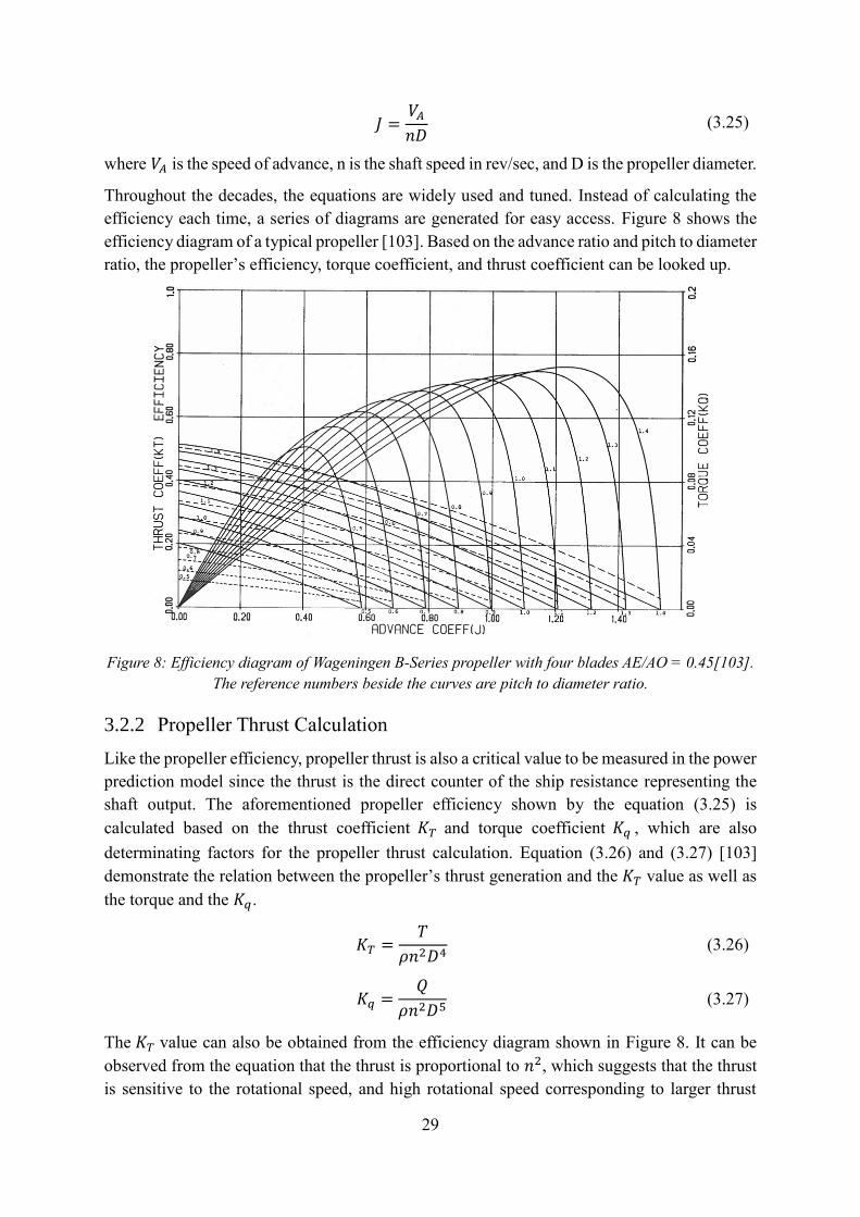
29
𝐽 =𝑉𝐴𝑛𝐷
(3.25)
where 𝑉𝐴 is the speed of advance, n is the shaft speed in rev/sec, and D is the propeller diameter.
Throughout the decades, the equations are widely used and tuned. Instead of calculating the
efficiency each time, a series of diagrams are generated for easy access. Figure 8 shows the
efficiency diagram of a typical propeller [103]. Based on the advance ratio and pitch to diameter
ratio, the propeller’s efficiency, torque coefficient, and thrust coefficient can be looked up.
Figure 8: Efficiency diagram of Wageningen B-Series propeller with four blades AE/AO = 0.45[103].
The reference numbers beside the curves are pitch to diameter ratio.
3.2.2 Propeller Thrust Calculation
Like the propeller efficiency, propeller thrust is also a critical value to be measured in the power
prediction model since the thrust is the direct counter of the ship resistance representing the
shaft output. The aforementioned propeller efficiency shown by the equation (3.25) is
calculated based on the thrust coefficient 𝐾𝑇 and torque coefficient 𝐾𝑞 , which are also
determinating factors for the propeller thrust calculation. Equation (3.26) and (3.27) [103]
demonstrate the relation between the propeller’s thrust generation and the 𝐾𝑇 value as well as
the torque and the 𝐾𝑞.
𝐾𝑇 =𝑇
𝜌𝑛2𝐷4 (3.26)
𝐾𝑞 =𝑄
𝜌𝑛2𝐷5 (3.27)
The 𝐾𝑇 value can also be obtained from the efficiency diagram shown in Figure 8. It can be
observed from the equation that the thrust is proportional to 𝑛2, which suggests that the thrust
is sensitive to the rotational speed, and high rotational speed corresponding to larger thrust

30
generation. However, the situation only holds when the thrust is aligned with the sailing
direction. To be discussed in detail in later sections, the current M-LOM considers only the
sailing direction. Such a propeller thrust calculation method may induce large errors during the
vessel’s departing and approaching phase where the propeller may be angled for ship turning.
Except for the empirical equation shown previously, propeller thrust can be obtained through
CFD simulation as well. Section 3.4.2 shows the CFD simulation for extracting the propeller
thrust and torque for efficiency calculation.
3.3. Modified Low-Order Model and Calculation Method (M-
LOMCM)
3.3.1 Model Related Work
The low-order ship resistance model and calculation method is based on the regression
approach that originated from the method published in 1982 by Holtrop and Mennen. The
technique is developed through regression analysis based on the full-scale data from the
Netherlands Ship Model Basin [95].
In Holtrop and Mennen’s original work [95], the total hull resistance is subdivided into the
following parts:
𝑅𝑇 = 𝑅𝐹(1 + 𝐾1) + 𝑅𝐴𝑃𝑃 + 𝑅𝑊 + 𝑅𝐵 + 𝑅𝑇𝑅 + 𝑅𝐴 (3.28)
where, 𝑅𝑇 is the total resistance, 𝑅𝐹 is the friction resistance, 1 + 𝐾1 is the hull form factor,
𝑅𝐴𝑃𝑃 is the resistance of appendages force, 𝑅𝑊 is the wave-making and wave-breaking
resistance, 𝑅𝐵 is the additional pressure resistance of a bulbous bow near the water surface,
𝑅𝑇𝑅 is the additional pressure resistance of immersed transom stern, and 𝑅𝐴 is the model-ship
correlation resistance.
Aiming at predicting the propulsion power of high-block ships with low length to beam ratio
or slender naval ships, the method provides a series of empirical equations that can be
implemented without significant modification.
The method was adopted as a part of the M.A.Sc. research by Jaster [100]. The method was
detailedly reviewed in Jaster’s thesis, and a Simulink model was built for the study on a coast
guard ship (formerly known as the RV Tsekoa II) and performance evaluation. Then, the
method was implemented in the MATLAB environment by Mostafa Rahimpour during the
research of the Transport Canada Clean Transportation project [29]. The model was not fully
established since the alternative reduced-order model was proposed; however, a series of CFD
was performed for evaluation on the BCFS ship Skeena Queen and Klitsa.

31
Figure 9: Comparison between the dedicated ship drag regression and numerical results [101]
In this study, a modified low order hull resistance and calculation method is proposed. The
model is based on Holtrop and Mennen’s (H&M) regression equation illustrated in section
3.1.1. There are three reasons for using H&M’s method as the backbone of the modified model:
a) Time-consuming and costly full-scale CFD, sea trial, and towing tank methods can be
avoided when using H&M’s method. The regression relationship is obtained through
full-scale sea trial data, which by itself is a hydrodynamic model. When configurated
with the designated ship’s parameters, the hull resistance can be predicted in a short
period (in order of hours for the whole process). Although the level of fidelity is low
compared to other methods, the results are critical and sufficient for industries to use at
the early ship design phase.
b) The method takes the ship’s velocity, hull geometry data, and stability data as input,
which are accessible at the early ship design phase. The required parameters can be
captured through CAD models, one-pass pre-calculated CFD, and designed ship sailing
conditions, which enhance the benefit of the method during its application at ships’
design phase.
c) As a calculation method, the model can be integrated as MATLAB functions or
Simulink model. Such a characteristic is critical for integrated model-based system
design and optimization. Since the control strategy is optimized during MBD, the power
prediction model needs to be embedded in the system to determine the global optimized
components’ working conditions, power ratings (component size), and control schemes.
To extend the original H&M’s method and increase the level of fidelity, the upper deck wind
drag calculation is added to the model. Using the Beaufort wind scale method illustrated
previously, the wind resistance can be estimated without sea trial data.
After the method is proposed, it needs to be constructed and tested using real ferry operation

32
data. The detailed model implementation is introduced in section 3.5, the remaining work in
this section is to illustrate the procedures used for the ship’s stability characteristic prediction
using one-pass CFD.
3.3.2 Numerical Estimation of Stability Characteristics Using CFD
The benchmark ferry used for model developments and results validations is BC Ferry’s
Tachek, a roughly 50 meters long passenger/vehicle and cargo ship connecting Quadra Island
and Cortes Island. The ship was built in 1969 with all documents, such as the stability booklet,
available. The implementation includes CFD based stability data calculation, wind resistance
model implementation, propeller efficiency model implementation, and results cross-validation.
The Tachek voyage data used is collected by Zhu during his M.A.Sc. research work, as
mentioned in [30]. The raw data is processed in Excel and imported into MATLAB as a discrete
time table data type. The used data contains time, ship speed in knots, port shaft speed in RPM,
port shaft torque in kN, starboard shaft speed in RPM, and starboard shaft torque in kN.
As aforementioned, the required stability data includes the center of buoyancy and draft, which
are often listed in the vessel trim and stability booklet. When the booklet is missing or
undetermined since no physical ship not yet available, such data needs to be calculated from
the mathematical equation, measured from the CAD model, and computed from CFD
simulation. To obtain this information, CAD models and loading conditions need to be
available.
The processes for calculation the stability data include the following steps:
a) Measure the location of the center of the gravity of the whole ship (require simple CAD
modelling to create ship’s upper deck geometry)
b) Based on the weight distribution and loading condition, estimate the still water volume
of displacement based on the conventional buoyancy force equation.
c) Measure the hull volume corresponding to the water displacement to obtain the still
water draft
d) Based on the weight, CG location, and draft level, set up CFD for solving hydrostatic
position and hydrodynamic response for stability data.
The first step is to estimate the ship’s center of gravity since it is critical for hydrostatic position
calculation. Among all three dimensions, the transverse and lateral CG position is more critical
for the situation since it influences the center of buoyancy, which is a determinating factor for
the hydrostatic calculation. In order to estimate the CG position, the CAD model is constructed
first. The hull model is created by Micheal Grant based on the geometric hull data provided by
BC Ferries during the study for Transport Canada [29]. The upper decks are modelled based
on the side views, section views, and floor plans provided by BCFS. The creation of the upper
deck can also help with the surface area estimation during wind resistance calculation. The
loading condition is assumed to be full load departure, which suggests the vehicle and
passengers are fully loaded, and the fuel oil tanks and freshwater tanks are 98 percent full. Such
a loading condition is for simulating the extreme situation where the maximum power demand
may occur. The model is constructed using the NX platform, as shown in Figure 10.

33
Figure 10: Rough CAD model for Tachek upper decks
The CG measurement shows the CG location to be (-361.4mm, -9.2mm, 5835.5mm) in x,y,
and z from the center of the ship, whereas the stability booklet indicates the CG is at (-557.8mm,
-2.1e-2mm, 5175.5mm). Comparing the results, a 35 percent error can be noticed for the
longitudinal location of the CG. However, the absolute error is insignificant considering the
length of the ship, the error can be ignored.
Figure 11: NX CAD model measurement report
Under the loading condition, the total weight of the ship is 715388.5 kg. Therefore, the still
water draft level can be roughly estimated using the conventional buoyancy equation:
𝐹𝑓 = 𝜌𝑤𝑎𝑡𝑒𝑟𝑉𝑑𝑖𝑠𝑝𝑙𝑎𝑐𝑒𝑚𝑒𝑛𝑡𝑔 (3.29)
Considering ocean water density to be 1024 𝑘𝑔/𝑚3, the volumetric displacement of the ship

34
is 698.6 𝑚3. After measuring the corresponding volume and height from the CAD model, the
draft is obtained to be 2.495 m (8.185 ft), which is close to the given 2.515 m (8.25 ft) levelled
water draft.
Figure 12: Measure the corresponding volume for determining draft
The calculated draft is then plugged into the Ansys Aqwa toolbox to evaluate the hydrostatic
position and hydrodynamic response. The whole setup and results report is shown in Figure 13
and Figure 14. The result longitudinal center of buoyancy is -1.674 m, and the vertical CB is
1.589, whereas the given data is -1.703 m (5.59 ft) for longitudinal CB and 1.6 m (5.25 ft) for
the vertical CB.
Figure 13: Ansys Aqwa hydrodynamic diffraction set up
Figure 14: Ansys hydrostatic position results report

35
Except for the Ansys Aqwa toolbox, the conventional NX CFD solver, Ansys Fluent, and NX
FloEFD are also tested for the CFD simulation. The following section briefly summarizes the
tested packages.
Conventional NX CFD Package
NX built-in CFD is able to calculate the drag force of the hull; however, the calculations are
for still water. Meanwhile, the conventional CFD cannot solve for the hydrostatic position of
the ship hull. Therefore, the draft, center of buoyancy, and other stability data cannot be
calculated. When performing the analysis, the draft has to be manually modelled. To evaluate
the draft, a similar approach to the aforementioned method using in Ansys Aqwa is necessary.
However, the center of buoyancy can not be assessed since no build-in feature is available.
Figure 15: Conventional build-in NX CFD solver setup
FloEFD Toolbox for NX
FloEFD toolbox has more robust functionality than the conventional package. With the ability
to define water and air condition, the program can generate a series of results, including surface
drag, volumetric drag, and structural results. However, the program still cannot produce a
hydrostatic position. Since UVIC does not have a toolbox license, a trial version was tested on
a virtual desktop provided by the vendor. Since no file exchange can be made, a simple drafted
model is tested instead of a hull model. With the free flow surface function (similar to
SolidWorks wizard), the program is able to simulate ships in water conditions. However, due
to the limited tutorial provided, a lot of the functions can not be performed. After testing,

36
FloEFD is stronger than the conventional CFD package; however, most of the functions do not
aim for hydrostatic or hydrodynamic analysis of a floating body.
Figure 16: FloEFD NX version simulation setup and results
Ansys Aqwa
Ansys Aqwa is capable of solving the hydrostatic and hydrodynamic response of the hull. For
a given draft, the program can calculate the center of buoyancy; however, the disadvantage is
that the program requires a center of gravity value input. The program can evaluate the CG
based on the geometric and material; however, with the absence of the upper-level components,
the evaluated CG is for the hull. If used, the center of buoyancy cannot be accurately estimated.
Explicitly designed for float object hydrodynamic analysis, Aqwa can evaluate the floating
behaviours under the impacts of waves, currents, and winds. In addition, other stability data,
such as the righting arm, can be calculated. However, when testing, it is found that Aqwa
mainly calculates the passive response of an object under conditions such as waves. Ship speed
cannot be defined, and the propeller cannot be set to rotate to see the propulsion force.

37
Figure 17: Ansys Aqwa simulation setup. The Ansys is able to implement the wave representation for
solving the hydrodynamic model.
The major problem is that the system cannot calculate the draft. A test is performed by leaving
the hull above the water surface and define the material properties and gravity. The purpose is
to check if the program will reach the hydrostatic equilibrium, and thus draft can be evaluated;
however, the program failed to assess the system and resulted in a 0 draft result. Therefore, the
draft needs to be manually modelled prior to the hydrostatic simulation.
Ansys Fluent
Ansys Fluent is a well-developed and commonly used CFD package. Similarly, Fluent is able
to calculate for the hull surface drag and other related fluids conditions; however, hydrostatic
is still not obtainable using Fluent.
Figure 18: Ansys Fluent setup and results

38
3.4. Modified Low Order Propeller Thrust/Torque/Speed Model
After obtaining the vessel hull resistance, the ship’s primary propulsion power can be estimated
through the products of resistance force and velocity. However, the effective propulsion power
(propulsion shaft power) is the more critical parameter to be measured for propulsion system
design since its quantity directly affects the propulsion component's sizes. In order to get
effective power, propulsor related data such as propeller’s efficiency, operational coefficients,
and torque/speed/thrust combination are necessary. This section illustrates a modified Holtrop
and Mennen’s drag based vessel surging power deduced model for predicting vessels’ effective
propulsion power utilizing the resistance characteristic and propeller related information.
3.4.1 Modified Holtrop and Mennen’s Drag Based Surging Power Deduced
Model
By its name, the proposed surging power deduced model is constructed based on the previously
obtained vessel’s resistance results using the modified H&M low order model and calculation
method. Differ from the conventional propeller thrust models where the propeller thrust is
calculated, the deduced model assumes that if the propeller produced thrust is known, the
effective propulsion power can be calculated using the equation
𝜂 =𝑝𝑟𝑖𝑚𝑎𝑟𝑦 𝑝𝑟𝑜𝑝𝑢𝑙𝑠𝑖𝑜𝑛 𝑝𝑜𝑤𝑒𝑟
𝑒𝑓𝑓𝑒𝑐𝑡𝑖𝑣𝑒 𝑝𝑟𝑜𝑝𝑢𝑙𝑠𝑖𝑜𝑛 𝑝𝑜𝑤𝑒𝑟=
𝑡ℎ𝑟𝑢𝑠𝑡 ∗ 𝑣𝑒𝑙𝑜𝑐𝑖𝑡𝑦
𝑡𝑜𝑟𝑞𝑢𝑒 ∗ 𝑟𝑜𝑡𝑎𝑡𝑖𝑜𝑛𝑎𝑙 𝑠𝑝𝑒𝑒𝑑
(3.30)
In order to use the equation to find the effective propulsion power, the propeller thrust and
efficiency need to be calculated.
Instead of calculating the thrust from the propulsor, the method considers the Newton second
law. The model assumes that considering only surge direction, the total amount of thrust needed
for propulsion is equal to the sum of total resistance and mass acceleration. For the Tachek
ferry, the acceleration can be obtained through the derivative of the velocity data. Combined
with the assumed full-load departure loading condition, the mass acceleration can be predicted.
The total ship resistance can be estimated using the previously introduced low order model and
calculation method. Hence, the total thrust can be calculated. Once the propeller efficiency is
obtained, the effective propulsion power can be deduced.
Several assumptions are made for such a deduced method:
The thrust is assumed to have the same direction as the velocity, which is all in the surge
direction. Under this assumption, the method only contains 1 DOF, which is the same
as the modified low order model and calculation method. In consequence, the level of
fidelity is low and the method belongs to the low order category.
Since no maneuvering is not captured in the model, the thrust amount from each
propeller is considered to share the total thrust equally.
To achieve deceleration, thrust from the opposite direction is considered.
With the total amount of thrust estimated, the most critical process falls on propeller efficiency
calculation.

39
3.4.2 Pre-calculated Propeller Efficiency
As reviewed in the previous section, propeller efficiency is governed by equation (3.24). For
this study, three methods are tested and compared to find the best way to obtain the propeller
efficiency.
Direct Efficiency Calculation
To directly calculate the propeller efficiency, equation (3.24) is added to the original LOM. The
equation requires the torque and thrust coefficient, which are illustrated in the Appendix. An
additional line of code is used to calculate the advance ratio. The pseudo-code reads as:
1 for each discrete vessel speed data
2 Set propeller diameter to 1.83 m
3 Calculate discrete ship wake fraction
4 Calculate discrete ship advance speed
5 Calculate the discrete advance ratio based on shaft rotational speed
6 Calculate torque and thrust coefficient
7 Calculate propeller efficiency based on thrust and torque coefficient and advance
ratio
8 If efficiency > 1|| efficiency <0
9 Correct the efficiency to 0
10 end
11 end
The calculation is done in matrix form since both port and starboard efficiencies are considered.
The method requires actual ship speed and shaft speed as input. The remaining two methods
also require the speed data and partial shaft speed as input. Later studies show that the ship’s
speed is a mandatory input, whereas the propeller’s rotational speed can be replaced by the
propeller designed rotational speed. The details are discussed in the Model Validation section.
Efficiency Diagram Lookup
Based on the Tachek propeller geometry, the propeller efficiency is read from Figure 8. Figure
19 shows the resulting propeller efficiency for the Tachek propeller.
It is worth noting that Figure 8 shows the efficiency of the Wagentingen B series propeller, a
typical water propeller geometry, with four blades and 𝐴𝐸/𝐴𝑜 = 0.45. The Tachek propeller
also belongs to the B series propeller; however, the ratio of the propeller’s extended area and
disk area for the Tachek propeller is 0.43, which is not an exact match to the diagram used.
Thus, further interpretations are used to capture the area ratio and the 0.87 pitch diameter ratio.

40
Figure 19: Tachek propeller efficiency based on the efficiency diagram
Base on the obtained data points, a 1-dimensional lookup table with linear interpretation is
constructed in the original LOM file with the discrete advance ratio as input and propeller
efficiency as output. The advance ratio is previously calculated during the direct calculation
method, which can be adopted here. Table 2 shows the tabulated value used for the 1-
dimensional interpretation. In between each data point, linear interpretation is used for
approximation. If the calculated advance ratio is beyond the boundary, the efficiency is taken
to be 0.
Table 2: Propeller efficiency lookup table for function implementation
Advance Ratio Propeller Efficiency Advance Ratio Propeller Efficiency
0 0 0.55 0.583
0.05 0.065 0.6 0.62
0.1 0.125 0.65 0.645
0.15 0.2 0.7 0.67
0.2 0.245 0.75 0.667
0.25 0.307 0.8 0.64
0.3 0.359 0.85 0.605
0.35 0.415 0.9 0.52
0.4 0.46 0.95 0.28
0.45 0.515 1 0
0.5 0.545
0
0.1
0.2
0.3
0.4
0.5
0.6
0.7
0.8
0 0.2 0.4 0.6 0.8 1 1.2
Pro
pel
ler
Effi
cien
cy
Advance Ratio
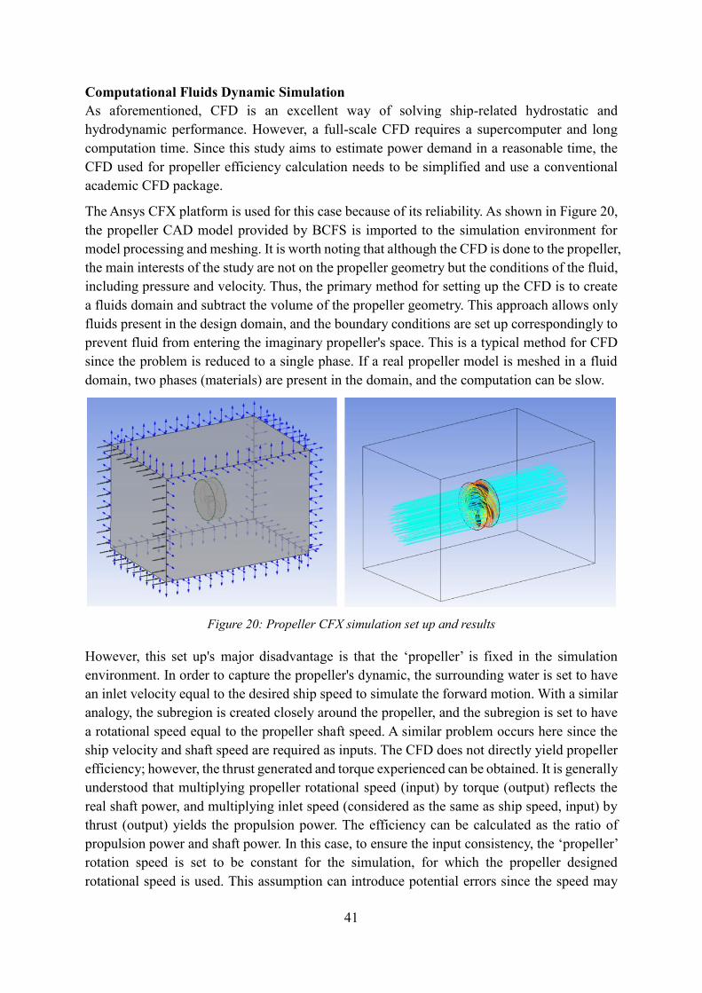
41
Computational Fluids Dynamic Simulation
As aforementioned, CFD is an excellent way of solving ship-related hydrostatic and
hydrodynamic performance. However, a full-scale CFD requires a supercomputer and long
computation time. Since this study aims to estimate power demand in a reasonable time, the
CFD used for propeller efficiency calculation needs to be simplified and use a conventional
academic CFD package.
The Ansys CFX platform is used for this case because of its reliability. As shown in Figure 20,
the propeller CAD model provided by BCFS is imported to the simulation environment for
model processing and meshing. It is worth noting that although the CFD is done to the propeller,
the main interests of the study are not on the propeller geometry but the conditions of the fluid,
including pressure and velocity. Thus, the primary method for setting up the CFD is to create
a fluids domain and subtract the volume of the propeller geometry. This approach allows only
fluids present in the design domain, and the boundary conditions are set up correspondingly to
prevent fluid from entering the imaginary propeller's space. This is a typical method for CFD
since the problem is reduced to a single phase. If a real propeller model is meshed in a fluid
domain, two phases (materials) are present in the domain, and the computation can be slow.
Figure 20: Propeller CFX simulation set up and results
However, this set up's major disadvantage is that the ‘propeller’ is fixed in the simulation
environment. In order to capture the propeller's dynamic, the surrounding water is set to have
an inlet velocity equal to the desired ship speed to simulate the forward motion. With a similar
analogy, the subregion is created closely around the propeller, and the subregion is set to have
a rotational speed equal to the propeller shaft speed. A similar problem occurs here since the
ship velocity and shaft speed are required as inputs. The CFD does not directly yield propeller
efficiency; however, the thrust generated and torque experienced can be obtained. It is generally
understood that multiplying propeller rotational speed (input) by torque (output) reflects the
real shaft power, and multiplying inlet speed (considered as the same as ship speed, input) by
thrust (output) yields the propulsion power. The efficiency can be calculated as the ratio of
propulsion power and shaft power. In this case, to ensure the input consistency, the ‘propeller’
rotation speed is set to be constant for the simulation, for which the propeller designed
rotational speed is used. This assumption can introduce potential errors since the speed may

42
not correspond to the specific velocity input. The possible effects are discussed in the following
section.
Model Comparison
The yielded efficiency curves are plotted in Figure 21 to compare the outcomes from three
methods. Results from the three methods showed no significant variance, and the largest
difference is 3 percent.
Figure 21: Results of three tested propeller efficiency calculation methods
There are several issues associate with each method. For the empirical equation method, the
equation can lose its meaning when certain conditions occur. For example, when the ship is
docking, propellers remain operating to generate thrust to push the vessel against the dock.
However, the ship velocity is 0 during the stage, and the propeller efficiency is 0 based on the
equation. To estimate the shaft power, the equation must divide the propulsion power by
efficiency. In this case, division by zero will occur, resulting in an infinity shaft power demand
while docking. This division is not feasible nor correct; however, the actual efficiency is not
measurable. The situation is similar to the remaining methods. When the advance ratio is zero,
the lookup table yields 0 for the efficiency, whereas CFD calculates the shaft power, but the
propulsion power is zero; hence the efficiency is 0. Currently, the results are tuned by using a
conditional division to eliminate dividing by zero situation. However, a method for solving the
problem is required and needs further investigation.
On the other hand, the opposite situation occurs when the ship’s speed is high and the propeller
speed is low. Usually, when a vessel sails in a straight line, the ship speed increases when the
propeller speed increases. However, during maneuvering, one side of the propeller may reduce
velocity for turning. Such velocity difference will result in low shaft speed accompanied with
high ship speed, and after calculation, the obtained propeller efficiency can be greater than one.
0
0.1
0.2
0.3
0.4
0.5
0.6
0.7
0.8
0 0.2 0.4 0.6 0.8 1 1.2
Effi
cie
ncy
Advance Ratio
Equation
Lookup
CFD

43
The problem associated with the CFD simulation is the shaft speed input. The designed
propeller speed is used as a fixed input to shaft speed, yielding consistent results comparable
to the empirical equation and lookup table method. The obtained operation data of the Tacheck
have paired shaft speed and vessel velocity. However, the CFD simulation results could not
produce the matched vessel velocity with the given propeller shaft speed as input. The method
of using one fixed shaft speed for propeller efficiency calculation to cover all vessel velocity
needs to be further investigated.
The propeller efficiencies are calculated using both real shaft speed and fixed design speed to
test the problem. The measured shaft power is then multiplied by the two different sets of
efficiencies to calculate propulsion power. In Figure 22, the blue line illustrates the propulsion
power estimated using the real shaft speed, and the red line shows the power obtained using
the fixed shaft power. A small disagreement with a maximum of 17 percent difference can be
observed. Since the ferry with a well-defined mission cycle continuously sails at its design
speed, the estimation presents a small error. A large error is expected for vessels with
dynamically changing velocity and associated shaft speed. At the early design stage, the
constant shaft speed can be used to roughly estimate propeller efficiency.
Figure 22: Power results using fixed and real RPM. Blue is the recorded data, whereas red shows the
predicted results. The horizontal axis is time in [second], and the vertical axis is power in [W]
From the comparison, it can be concluded that using typical propeller speed as fixed input for
propeller efficiency is a feasible estimation. However, to have acceptable estimation results,
the ship's mission cycle should not have frequent fluctuation. For ferries with a “departing-
accelerating- cruising- decelerating- docking” type mission cycle, the estimation is feasible.

44
Considering three methods, the lookup table derived from the efficiency diagram is the best
method that should be implemented into the LOM. The equation calculation yields an
unexpected negative or greater than one efficiency value; the process can not provide consistent
results until the maneuvering is modelled in the LOM. The CFD method generates consistent
results; however, at least ten simulations need to be performed to obtain a full list of efficiency.
The time consumed by one-pass CFD is significantly less than full-scale CFD; however, each
run still required an hour to compute. Any modification can be time-consuming to achieve. The
efficiency diagram can be read to generate the lookup table, on the other hand. Throughout
decades of propeller design modifications and interpretation, the propeller designs have
become similar and can be generalized by several typical propeller geometries. An efficiency
diagram with the same number of blades and a similar Ae/Ao ratio can be used for estimation.
Meanwhile, with the empirical equation and CFD method, the lookup table method's accuracy
can be proved. However, with the conclusion made, if the corresponding lookup table is not
available, the CFD method needs to be performed since it can both calculate the efficiency as
well as help obtain the efficiency lookup table.
For a marine vessel, the propeller(s) can be the conventional fixed-end type or the azimuth type.
The former's pointing direction is fixed with fixed or variable pitch, while the latter can switch
its pointing direction to improve the vessel’s turning radius. With an azimuth propeller, the ship
can be maneuvered by changing the direction of the thrust. When rotating 360 degrees, the
advance ratio for the propeller is different for four quadrants. When the situation occurs, only
the direct calculation method can be used for obtaining the propeller efficiency since the sign
varies in different quadrants.
3.4.3 Iterative Propeller Speed Estimation Model
As aforementioned, the propeller designed rotational speed is used for the efficiency simulation.
The results are compared to the real measured data, and the accuracy is adequate. However, for
propulsion system design, the propeller required torque and rotational speed needed to be more
accurately calculated since the engine and motor output torque, speed, and power are needed
for component sizing and control strategy optimization. Therefore, estimating the propeller
speed is an essential next step of the work.
From Figure 8, the thrust coefficient can also be obtained based on the advance ratio. Equation
(3.26) illustrated the relation between the propeller generated thrust to the thrust coefficient.
According to the equation, assuming the thrust is equal to the predicted drag force, with 𝐾𝑇
available from the efficiency diagram, the propeller speed can be calculated accordingly. Figure
23 shows the interpreted thrust and torque coefficients for the Tachek propeller.

45
Figure 23: Tachek propeller thrust and torque coefficient
An iterative process is then undertaken to calculate the shaft speed to generate an equal amount
of thrust. The pseudo-code reads as following
1 for the amount of the data point
2 set propeller speed n to be 280 RPM and error to 10
3 while |error| > tolerance
4 calculate advance ratio
5 interpret thrust coefficient Kt and calculate thrust
6 error = calculated thrust – estimated drag
7 calculate the difference of n using yielded error
8 set n = n – dn
9 end
10 record calculated n for each data point
11 end
Figure 24 compares the measured shaft speed to the predicted shaft speed using the
backpropagation method. During the cruise sailing phase, the predicted shaft speed matches
the measured speed accordingly; however, a significant difference can be observed during the
departing and approaching phases. The reason for such difference is that the listed assumptions
suggest that all propeller power is transferred into propulsion power under particular
efficiencies and translated into ship speed. However, during the docking, leaving, and
approaching phases, a part of the power delivered by propellers is used for maneuvering as
well as stopping the ship. The predicted shaft speed is low since the ship’s speed is low during
0
0.005
0.01
0.015
0.02
0.025
0.03
0.035
0.04
0.045
0.000
0.050
0.100
0.150
0.200
0.250
0.300
0.350
0.400
0 0.2 0.4 0.6 0.8 1
KqKt
Advance Ratio
Kt
Kq

46
the stages. The maneuvering needs to be considered with additional DOFs to get a better-
matching result.
Figure 24: Comparison between measured shaft speed to the predicted shaft speed using the
backpropagation method. The horizontal axis indicates the time in [second], and the vertical axis
shows the shaft speed in [rads/s].
This study modified the existing low-order model and investigated the performance by
comparing the model predicted ship shafts power profile to the real measured shaft data on the
Tachek ferry. The model required inputs are obtained by solving well adopted empirical
equations, simulating using CFD, and directly measuring from the existing ship. The model's
overall accuracy is sufficient for powertrain design purposes since the peak, and continuous
power outputs match the recorded data. Several shortages impact the overall accuracy, which
will be discussed below in this section.
The active model captures almost all significant environment-induced resistance, including
hull resistance caused by viscosity friction, wave, current, and upper deck resistance introduced
by the wind. However, at the current model development stage, resistance direction is not
captured; all modelled resistance is assumed in the sailing direction. Vessel turning and
maneuvering is not considered in the model. This simplification vastly reduces the system
degree of freedom and the overall complexity, which dramatically improves the reduced-order
model without significantly damaging the accuracy. However, there is no doubt that inaccuracy
will be introduced since the various directions of current, wind, and wave can influence
performance, especially during the low-speed condition. Meanwhile, the direction of the forces
encountered and generated will impact the propellers’ efficiency, further introducing inaccuracy.
As mentioned, a 3 DOF system generates better results since maneuvering is a critical area to
be studied.

47
Similar to the water conditions, a few assumptions are made to simplify wind resistance
calculation. First of all, the wind is assumed to be a headwind during the entire sailing. The
wind direction affects the projected area, which is critical for wind resistance calculation. In
addition to the direction, the magnitude is considered to be constant during the entire sailing.
Jointly, the model yields a matching power profile; however, improvement can be expected
when DOF increases. And a more accurate power profile helps with the powertrain component
sizing and control design for energy management.
3.5. Software Implementation and Model Validation
The model related calculations, introduced in the previous two sections, have been
implemented as MATLAB functions, and this section details the formed Simulink models. An
existing MATLAB file was created by Mostafa Rahimpour that contains the original Holtrop’s
regression method [29]. The MATLAB codes are used as a baseline for implementing the
modification. From the comparison in Section 3.4.2, the lookup table method interpreted from
the efficiency diagram is used.
The inputs for the modified LOM includes:
Length on the waterline (LWL)
The length between perpendiculars (Lpp) (length of a ship along the waterline from
the forward surface of the stem)
Breadth moulded (B)
Average moulded draft (T)
Displacement volume moulded (Vd)
Longitudinal center of buoyancy (LCB) (forward +, aft -)
Draft moulded on F.P. (Tf)
Draft moulded on A.P. (TA)
Transverse bulb area (Abt)
Centre of bulb area above keel (hb)
Midship section area (Amid)
Waterplane area (Aw)
Transom area (At)
The wetted area of the hull (S)
Wetted area appendages (Sapp)
Bow thruster tunnel diameter (dbto)
Bow thruster tunnel openings coefficient (Cbto)
Beaufort wind scale (BN)
Design shaft speed (n)
Ship sailing speed (V)
The following flowchart depicts the process flows of the entire modified LOM. Figure 25 and
Figure 26 show the predefined functions to be called or run before the primary MATLAB
function, and Figure 27 shows the main function flow. The implemented code will be attached
to the Appendix.

48
Figure 25: Processes flow for the subfunction contains resistance and efficiency calculation
Figure 26: Predefined functions for setting up propeller efficiency lookup table and stability data
calculation

49
Figure 27: Main LOM function flow

50
After obtaining the predicted power profile, the results are compared to the real measure power
profile for accuracy evaluation. It is worth noting that measured data by M.A.Sc. Zhu [30]
reflects the real shaft power, which needs to be compared to the ratio of predicted propulsion
power and estimated propeller efficiency. However, as aforementioned, predicted efficiencies
contain zero when the ship is docking, a division by zero is not feasible. The measured shaft
power is multiplied by the propeller efficiency to yield an estimated propulsion power profile
for making the comparison. Then, the estimated propulsion power profile is compared to the
modified LOM's predicted propulsion power profile.
Figure 28 shows a comparison between the predicted and measured propulsion power profile.
The blue line shows the modified LOM generated results, whereas the red line is the results
obtained from the measured shaft power multiplied by the propeller efficiency.
Figure 28: Results comparison between predicted and actual measured shaft power profile. The
horizontal axis is time in [second], and the vertical axis is power in [W]
To quantify the difference between the predicted results and measured data, the mean absolute
percentage error (MAPE) between the two data sets is calculated. The MAPE is the average
percentage error between all data pairs, which is calculated as:
𝑀𝐴𝑃𝐸 =1
𝑛∑|
𝐴𝑖 − 𝑃𝑖𝐴𝑖
|
𝑛
𝑖=1
(3.31)
Using equation (3.31), the directly calculated MAPE is 35.88 percent. The difference is
partially caused by power output misprediction at the low-speed regions and a consistent minor
time delay of the prediction. For this quasi-static power loss based propulsion system
performance and energy efficiency models, the average power percentage errors are relevant.
When considering the average power output at departing, cruising, and docking phases, the

51
differences between the measured and predicted values are only 2.13, 0.06, and 4.58 percent,
respectively. During the cruising phase, which is the primary sailing period, the largest
mismatch is 9.09 percent, occurred at the bottom peak pointed out by the red arrow in Figure
28 during constant velocity sailing. The general trend of the two data sets is consistent.
On the other hand, it is crucial to measure the total power consumption difference between the
two data sets. The total power consumption affects overall fuel consumption and emissions,
which are two critical parameters for hybrid power train design since they are treated as
optimization objectives. The percentage difference in total power consumption between
measured and predicted data is at 2.12 percent. When considering the entire mission cycle, the
result suggests that the expected total consumed power matches the real data closely, even some
largely distinguished data points exist.
3.6. Key Improvements - Stability Data-Based Model
When comparing the calculation method to the other model mentioned, the pronounced
advantage is the computation time reduction without sacrificing accuracy. Figure 29 compares
the modified hull resistance model to the aforementioned resistance estimation models. The
sea trial and towing tank method require the physical ship or scaled prototype, whereas ROM
and full-scale CFD rely on high-intensity calculation. The advantage of the M-LOMCM is
finding the midpoint that balances the needs of software computation and the “physical” model.
Figure 29: Hull resistance models comparison visualization. The scale is used to compare the needed
model and computational power for each model. The further to the right, the more computational
resource is required. The more to the left, the more physical model is necessary
The modified model has several noticeable improvements. First of all, M-LOMCM extends the
original Holtrop’s method to formulate a complete vessel shaft power demand model based on
the hull resistance model and propeller thrust model. Since the original Holtrop’s regression
method only considers the still air resistance, the power profile estimation can be inaccurate
and can potentially lead to incorrect component size selections. Instead, the M-LOMCM
combines the full upper deck resistance with hull resistance to estimate the total ship resistance.
When the wind data is missing, the Beaufort wind scale is used to generalize the wind
conditions. The additional propeller efficiency model further upgrades the resistance model
into a power profile prediction model. The original models only measure the hull resistance,
which is less useful than the power profile when selecting components for the integrated system
design. The additional propeller thrust/efficiency model converts the load profile into

52
propulsion power and shaft power profile, which can be directly used for integrated ship
propulsion system design.
Secondly, with hull form geometry data from the computer-aided design (CAD) model and
parameters obtained from the CFD simulations, the M-LOMCM only requires speed data as
input. Unlike the methods mentioned previously, where information such as sea trial and
stability data is needed for computation, the M-LOMCM unlocks the potential of “soft
prototyping” during the ship’s early design phase. The speed data is generally measured from
the physical ships; however, the ship’s top sailing speed is often determined at the design phase.
A synthetic speed profile can be used as a reference for early-stage simulation. Meanwhile, the
velocity profile from the ships that belong to the same class can be used as a reference.
Third, contrasting from the other complex models or full-scale CFD, the 6 DOF RANS is
represented by low-order regression empirical equations, which vastly reduced the time needed
for computation. The regression method relies on empirical equations and parameters obtained
through the sea trial or experience. Such parameters are either not obtainable at an early stage
of ship design or inaccurate. The CFD method is proven to be accurate by numerous researches
and is able to deliver precise hydrostatic and hydrodynamic parameters. On the other hand,
only one-pass CFDs through conventional CFD packages are required with the enchantment of
the regression relation. Such simplification reduces the time and computational resources
needed for the full-scale CFD. Without a physical model, the required stability data can be
accurately obtained utilizing the CAD model and CFD simulation. A similar analogy can be
applied to the propeller, where a single-pass CFD is used along with empirical equations for
obtaining propeller efficiency without a prototype.
Lastly, M-LOMCM can be modified to customize for each ship. Unlike the mathematical
model, the M-LOMCM is not a generic representation. Instead, for each vessel with unique
hull and propeller designs and distinct mission cycles, the model can be applied to capture the
unique hull resistance and power demand associated with the mission. Meanwhile, the M-
LOMCM is well implemented as a module in the MATLAB/Simulink environment, which can
be used along with the model-based design process. Since the resistance and power profile
depends on the speed data, the power prediction may vary as the speed changes when the
system control varies. The modulized M-LOMCM can be implanted into the design model,
which is beneficial during the integrated system optimization.
To show the general relation, the proposed M-LOM can be visualized in Figure 30.
Figure 30: A simple representation of the low-order model

53
Chapter 4. Comparison of Different Marine Propulsion
Systems
The benchmark comparison is the most commonly adopted method to study the different
hybrid-electric propulsion system's feasibility and performance. The benchmark method selects
a typical plant and applies various internal components, controls, or optimizations. Based on
the different outputs, the comparison set's final results can be directly compared and visualized.
This chapter details the benchmark vessel selection and modelling of various propulsion system
comparison set, including direct mechanical drive, NG-electric drive, pure electric drive,
parallel electric hybrid, and series electric hybrid.
4.1. Selection of a Benchmark Marine Vessel – BCFS Skeena
Queen
In order to generalize the study, a representative benchmark vessel is needed. The first
consideration to be made is the vessel's type and the weight level when selecting the benchmark
vessel. Generally, the ships/vessels can be categorized into three major top-level groups: cargo
ships, passenger vessels, and special-purpose vessels.
As detailedly reviewed in the first chapter, passenger ships such as ferries induce a large amount
of pollution that needs immediate attention. With a strong correlation with the BC Ferries, the
research group has been working on passenger ferries and has critical ship hull and internal
components data. Due to the advantages listed, the BCFS ferry Skeena Queen (SKQ, shown in
Figure 31) is selected as the benchmark vessel. The SKQ sails between Victoria and Salt Spring
Island, BC. The overall vessel specs are listed in Table 3.
Figure 31: BCFS MV Skeena Queen [107]

54
Table 3: BCFS MV Skeena Queen design details [107]
Built: 1997, Vancouver
Overall Length: 110 meters
Maximum Displacement: 2942 metric tonnes
Car Capacity: 92
Passenger & Crew Capacity: 450
Maximum Speed: 17.3 knots
Horsepower: 6000
Unlike ferries such as Tachek that use typical fixed-direction propellers at the vessel's stern,
the SKQ utilizes four azimuth propellers for both propulsion delivery and maneuvering. Such
a layout is beneficial since the propellers can be orientated into the heading direction, under
which condition the propeller efficiency can be maximized. Meanwhile, with four propellers
in place, the ferry has enough redundant propulsors to meet the regulations, where at least two
propellers must be under operation during the crossing [107].
The main focus of this thesis study is to use M-LOM in a complete vessel modelling process.
The M-LOM is constructed initially based on the Tachek ferry. And in fact, the M-LOM
performs better on the fix-direction propeller ship since the algorithms used for M-LOM
propeller efficiency calculation only serves in surge direction. Because the SKQ varies the
propellers’ facing direction during the operation, the additional DOF makes M-LOM not ideal
for the SKQ. However, the primary reason for selecting SKQ as the benchmark vessel is that
some previous studies have been done on the ship. As mentioned in Chapter 3 of the thesis, the
reduced-order ship hull resistance and propeller thrust model has been developed for the SKQ.
The ROM serves as an excellent reference set for the M-LOM used in this study. Meanwhile,
a dynamic model is available for the SKQ. When using the dynamic model, the research can
predict the propulsion power only based on the speed profile. Without using additional
measured data, the study can mimic the processes during the ship design phase, which is more
generalized and representative.
To systematically analyze the hybrid-electric propulsion system's performance, comparisons to
other conventional systems are essential. At the current stage, the ship design is volumetric
driven, under which condition, the most volumetric dense fuel such as marine diesel or
compressed NG is commonly used. Thus, the direct NG-mechanical drive through the internal
combustion engines is to be modelled as a comparison set. Meanwhile, diesel-electric is more
widely adopted on many ships to replace the conventional pure mechanical drive. In this case,
an NG-electric drive is considered as another benchmark comparison set to match the NG ICE.
With additional ESS in either parallel or series, the hybrid electric propulsion systems can be
achieved. Both series and parallel architectures will be modelled for performance comparison.
Lastly, a battery-driven pure electric propulsion system will also be compared.
The mainframe of the multiphysics model is shown in Figure 32. The only external input used

55
in the model is the vessel’s speed profile. Using the modified low-order ship hull resistance
model and calculation method, the corresponding thrust demand can be estimated. Based on
the ship’s speed, acceleration, and thrust demand, the modified low-order surging power
deduced model can calculate the propellers’ required power input. Meanwhile, the thrust value
is used by the ship dynamic model to predict the ship’s speed as feedback and comparison. The
propeller power demand is then carried on in the propulsion system model to compute the
engines and/or motors’ power demand, which can be translated into energy consumption. The
consumed energy can be finally transferred into the equivalent amount of fuel for the final
comparisons.
Figure 32: Integrated propulsion system design processes using low-order model
A few assumptions are made to simplify the model:
a) It is considered that the required thrust is evenly distributed among all four propellers.
The advantage of the SKQ system is that four propellers can be individually controlled
to achieve maximum efficiency. Ideally, to ensure torque balance, bow and stern
propellers can be controlled respectively to achieve front, rear, or all four-propeller
drive based on the driving condition. However, if the number of propellers in operation
changes, the working propellers’ speed and torque need to be changed. Additional
gearbox shifts are required to maintain system efficiency, which brings another layer of
complexity during the optimization phase. Hence, at the current stage, the four-
propeller drive is considered during the entire crossing.
b) Since the electric related information such as voltage, current, power, and efficiency
curve are not available for all components, no electric conversion can be simulated.
Ideally, the electric converter needs to be modelled to regulate the voltage and current
input/outputs for the motor and generator.
c) As mentioned before, the simulation is built up for only surge direction. This
assumption will lead to less accurate results for the SKQ ferry since the azimuth

56
propellers utilize a part of the thrust for maneuvering.
d) For the entire study and comparison, the SKQ ferry is considered to sail at a fully loaded
departing condition. The condition suggests the ferry is fully loaded with passengers
and vehicle, and the fuel tank and fresh water tank is full. The full loading condition is
for testing the extreme sailing condition.
e) For the entire simulation, only propulsion power is considered. The hotel loads are not
included due to the lack of data. For example, for some configurations, the series hybrid
electric drive, additional hotel loads can result in different NG generator operation
points, which could yield different fuel consumption results.
f) The electric energy is converted equivalently to fuel consumption for direct comparison.
A direct conversion based on fuel energy content and the amount of electric energy
usage are considered in this simulation. By dividing the electric power by the fuel heat
value, the fuel rate can be estimated. The estimated total equivalent fuel consumption
can be generated after cumulative integration over the time steps. Comparing to the
Equivalent Fuel Consumption Method established by Paganelli et al. [108], the used
conversion is a direct simplification. Different optimization methods rather than EFCM
are used and detailedly discussed in Chapter 5.
g) In the benchmark models, battery degradation is not considered. The degradation is
more related to system power control and energy management, which will be included
in a full case study shown in Chapter 5.
h) DC buses and DC components are used in all modelling processes. Due to the lack of
internal component parameters, conversion losses and phase requirements are hard to
determine. The DC bus allows direction efficiency assumption so that the overall model
is more consistent.
4.2. Natural Gas (NG) Engine Mechanical Drive
The conventional propulsion system with NG fueled engine(s) and mechanical drive is
modelled based on M.A. Sc. Zhu's engine data collected during his thesis research [30]. The
overall mechanical model is constructed and shown in Figure 33. According to the assumptions,
the propeller evenly delivers the required thrust; hence, only one propeller is modelled. The
thrust result is multiplied by four and returned to the vessel dynamics model for velocity
simulation. The individual propeller power requirement is transferred to the NG engine through
a gearbox. The final fuel consumption can be measured and multiplied by four to yield total
fuel consumption.

57
Figure 33: Benchmark model for the NG-mechanical drive propulsion system
The propeller block contains the M-LOM shown in Figure 34. As mentioned in Chapter 3, the
resistance model computes the overall hull resistance based on stability characteristics and
regression model. The required amount of thrust is the sum of the resistance force and mass
acceleration. The surging power deduced model computes the propeller’s rotational speed,
torque, and efficiency based on the thrust demand and advance ratio. It is worth noting that the
propeller block is identical for all configurations and will not be introduced again when
illustrating other configuration models.
Figure 34: The low-order model block representation
The data accusation block reads the input data from the workspace. The only used external
input is the ship’s velocity, which is compared to the predicted speed at the end by computing

58
the absolute error. The engine sizing is governed by the maximum power requirement of the
propeller, which is 650 kW. The gearbox block only contains one stage of gear reduction with
95 percent constant efficiency. The gear ratio is calculated based on the propeller’s speed under
the cruising stage. During the cruising stage, the ship is sailing at 17 knots, under which
condition, the propeller is rotating at 22 rad/s (210 RPM). Based on the scaled engine efficiency
curve, the adequate engine speed is around 115 rads/s (1098 RPM, corresponding to the high-
efficiency zone). Therefore, the gearbox ratio is selected to be 5.2 steps up. The engine model
is constructed based on the lookup tables. Since the model uses a backward approach, the
engine dynamic can be neglected. The fuel consumption can be looked up in tables and
integrated over the simulation time.
4.3. Natural Gas Engine Electric Drive
The NG-electric drive benchmark (shown in Figure 35) is similar to the mechanical drive
version, except an additional motor needs to be modelled. The motor model is based on the
commonly used TM4 electric machine with a scale specific to the propeller demand. The NG-
electric drive requires additional energy converters such as DCDC or ACAC to regulate the
voltage and current between the NG generator and electric motor. However, the available motor
data does not contain current, voltage, and efficiency curve; thus, control based on the electric
current and voltage is not feasible. Therefore, all the simulation is based on torque, speed, and
power efficiency instead. Without having information about the voltage and current, the
converter performance cannot be modelled, and the efficiency can only be assumed to be
constant 95 percent.
Figure 35: Benchmark model for the NG-electric drive propulsion system

59
Figure 36: NG generator block representation. The NG generator sub-block contains NG ICE,
gearbox, and electric generator.
The NG engine generator is modelled as the engine and motor combination, as shown in Figure
36. In the NG engine generator subblock, a forward approach is considered. The required power
is substituted into the engine block, and the resulting torque and speed data are then passed to
the gearbox and motor to yield the final power output. Based on the motor operation curve and
efficiency, motor efficiency is looked up along with the power output. The efficiency serves as
feedback to the power demand input to adjust the input in order to cover the power losses
during the processes.
4.4. Pure Electric Drive
The pure-electric drive configuration, shown in Figure 37, is almost identical to the NG-electric
drive, except the electric power is provided by a grid-charged battery ESS rather than from the
NG engine generator. The subblock ESS model used in the study was developed previously by
Li Chen [52]. The battery model is constructed based on the A123 battery. The allowed battery
SOC range is selected between 40 percent and 90 percent to maintain a healthy battery
condition.
Figure 37: Benchmark model for the pure battery-electric drive propulsion system

60
4.5. NG Engine Hybrid Electric Drive
In terms of modelling, the hybrid electric configurations are the combinations of the previous
three benchmark configurations. However, with additional power sources, usually battery or
supercapacitor, the control strategy is necessary to distribute and allocate the energy output
between the ESS and the ICE. For the two benchmark models, a simple power follower control
is used to emphasize each hybrid architecture's characteristics. For the series hybrid
architecture, the NG generator(s) operate in a few best-efficient electric generation points. The
battery pack is responsible for providing additional energy for propulsion or consuming excess
energy for charging. On the other hand, the parallel architecture allows the engine and motor
to provide torque at corresponding synchronized speed jointly.
4.5.1 Series Hybrid Electric Drive
The series hybrid electric drive is modelled and shown in Figure 38. The controller allows the
NG generator to operate at 300kW, which can fulfill half of the propeller’s continuous power
demand. The battery pack releases or collects charges based on the difference between the
power demand and the constant generator power rated at 300kW.
Figure 38: Benchmark model for the series hybrid electric drive propulsion system
4.5.2 Parallel Hybrid Electric Drive
The parallel hybrid architecture (shown in Figure 39) keeps the original mechanical linkage
between the ICE and propeller shaft. The additional motor is attached to the shaft through the
gearbox. It allocates the power distributions between the ESS and ICE, but the controller also
ensures the output rotational speed from ICE and motor after gearbox reduction are identical.

61
Figure 39: Benchmark model for the parallel electric drive propulsion system
4.6. Benchmark Performance Comparison
To quantitatively compare the performance of all benchmark configurations, the same speed
profile is used in calculating fuel consumption. Optimization is carried out on each design to
compare the results with the best system components. A global optimization method, discussed
in detail in Chapter 5, is used to find the optimal engine size, motor size, and gearbox ratio that
minimize the equivalent fuel consumption. Table 4 illustrates the optimization goal and
simulation results.
Since the simulation only considers the equivalent fuel consumption, the electric drive can
achieve high efficiency with the correct motor size and gearbox ratio; hence, the battery-electric
drive has the lowest fuel consumption. As mentioned in the assumption, if battery degradation
or SOC penalty is given, the EV's final results can be higher. The NG-electric drive performs
the worst due to a few reasons. To regulate the electric voltage, current, and power input/output,
multiple stages of electric converters are necessary for the system. The conversion leads to
energy losses, which reduces the system's overall efficiency significantly. Meanwhile, since
only propulsion power is considered for the active simulation, the NG generator must
frequently switch operation points to meet the power demand. Typically, when the hotel loads
are considered, the NG generators operate at a fixed narrow region to maintain the output power
and phase.

62
Table 4: Optimized benchmark model result comparison.
Benchmark
Configuration Design Objective of Optimization Total (Equivalent)
Fuel Consumption
[kg]
NG engine mechanical
drive
Engine size
Engine to propeller gearbox ratio
170.05
NG-electric drive Electric motor size
Motor to propeller gearbox ratio
NG generator size
NG engine size
ICE to generator gearbox ration
Generator size
226.62
Series hybrid electric
drive
Electric motor size
Motor to propeller gearbox ratio
NG generator size
NG engine size
Internal engine to generator
gearbox ration
Generator size
Battery size
NG generator operation point
152.30
Parallel hybrid electric
drive
Engine size
Motor size
Multi-input gearbox ratio
Battery size
Engine operation point
123.50
Battery pure electric
drive
Electric motor size
Motor to propeller gearbox ratio
Battery size
73.54
The series hybrid configuration largely resolves the sub-optimal operating points issue that the
NG electric configuration encounters by adding a battery pack to the system. The control
strategy allows the NG generator to operate at a single high-efficiency point for power
generation, whereas the battery covers the power shortage at high efficiency. On the other hand,
excess power is consumed by the battery for charging. Overall, the system efficiency can be
maintained at a high level during the entire crossing; hence the fuel consumption is lower

63
compared to the NG-electric drive.
The parallel hybrid drive can be compared to the direct mechanical drive since both systems
have ICE operating at variant operation points. The mechanical drive is better for the active
simulation than the NG-electric drive since less energy formation conversion occurs. The best-
fit gearbox ratio and engine size are obtained through the global optimization method to
improve the mechanical drive performance. The parallel hybrid system has an additional motor
coupled with the engine to power the shaft jointly. With the additional assistant, the engine
operating points can be allocated on the best efficient curve. Unlike the series hybrid drive,
where the engine runs at the highest possible efficiency zone, parallel drive locates the
operation points to corresponding power with the highest efficiency. For example, regardless
of the power demand, the series drive aims at a high-efficiency zone, and the power output may
fall far below or above the demand. When the situation occurs, the shortage or excess is covered
by the battery. The parallel drive selects a power near the demand. The desired operating points
are chosen to be the most efficient speed and torque combination based on the power and speed
demand. The coupled motor covers the additional torque.

64
Chapter 5. Application to Integrated Hybrid Electric Ship
Design
In the previous chapters, the fundamental theory of hybrid electric ship propulsion has been
thoroughly introduced. With assistance from the developed M-LOM, integrated hybrid ship
propulsion can be designed with limited external data. By utilizing the benchmarks modelled
in Chapter 4, this chapter illustrates an integrated design of a hybrid electric vessel propulsion
system using BC Ferries’ ship Skeena Queen (SKQ) as the test platform. The work
demonstrates the model-based design processes, including data processing, low-order model
construction, model-based system design, system control, and system optimization.
5.1. Propulsion Power Prediction
As stated in Chapter 3, the vessel’s propulsion power profile is critical for the model-based
design. The power profile reflects the peak and continuous power demand of the sailing, which
is the driving factor of component sizing. Meanwhile, this power demand serves as a constraint
during model optimization and directly affects power distribution and energy management.
Power profile prediction is regarded as the first milestone of the propulsion system design. For
the previous studies done on the SKQ by the research group, the speed profile is obtained
through real-world measurement. This section of the work utilizes the aforementioned low-
order model on the SKQ to predict the required shaft propulsion power.
Detailed in Chapter 3, the low-order model first computes the ship water/wind-induced
resistance based on the hull geometry, loading conditions, and stability data. Then, combined
with the ship’s velocity data and acceleration, the rigid body propulsion power can be estimated.
Lastly, merging with the propeller efficiency, the final shaft power demand can be determined.
The M-LOM is developed under the MATLAB environment. However, to combine the model
with the simulation processes, a Simulink block needs to be constructed first. When developing
the M-LOM, it is assumed that the vessel’s stability data is not available. However, for the
SKQ ferry, the full stability data under different loading conditions are documented in the
stability booklet. Since a fully integrated model is to be constructed at this moment, more
accurate data from the stability booklet is used.
In terms of obtaining the propeller’s efficiency, the conventional lookup table method is not
feasible since the SKQ propeller is specially designed with duct around the blades. A series of
CFD simulation needs to be conducted for acquiring the propeller efficiency, torque coefficient,
and thrust coefficient curves with respect to the advance ratio. The propeller’s designed
rotational speed is not recorded on the drawing. The designed ship velocity is estimated first
when performing the CFD simulation. Based on the recorded data, the ferry is sailing at 14
knots during the cruising phase, under which condition, the propeller shaft operates at 800
RPM. Based on the shaft to engine speed reduction and the documented engine to propeller
speed ratio, the propeller is calculated to run at 285 RPM during the cruising. Naturally, the
propeller has the highest efficiency under the designed rotational speed. Meanwhile, to
maintain efficiency, the ship is often intended to sail with designed propeller speed. Based on

65
the analogy, the propeller’s design speed is estimated to be 285 RPM for the CFD simulation.
Figure 40: SKQ propeller parameter computation setup using Ansys CFX
Similarly, the propeller CAD model is obtained from BCFS, and the water surrounding is
modelled using the Simens NX. The propeller and water region are assembled in the Ansys
CFX environment. To mimic the propeller and ship motion under the water, an inlet speed is
set up as a control variable for representing the ship’s speed, and water-subregion rotational
speed is input to serve as the propeller’s speed. As mentioned, the controlled inputs for the
simulation is forward speed and rotational speed. As stated, the fixed rotational speed (285RPM)
is used for all simulations. The ship’s speed is ranging from 0 to 23 knots. Such a speed range
is investigated due to the disagreement between the CFD simulation result and the ferry sailing
speed. The SKQ sails at 14 knots regularly during the cruising phase as recorded; however, the
CFD suggests that the propeller has the highest efficiency at 17 knots. Such disagreement
affects the designed propeller speed input; but, the issue is resolved by performing the propeller
speed backpropagation. The propeller’s efficiency, torque coefficient, and thrust coefficient
curves are shown in Figure 42.
Figure 41: SKQ propeller efficiency results from Aqwa CFD simulation. The horizontal axis
represents the propeller’s advance ratio, and the vertical axis shows the corresponding efficiency.
0.0000
0.1000
0.2000
0.3000
0.4000
0.5000
0.6000
0.7000
0.0000 0.2000 0.4000 0.6000 0.8000 1.0000 1.2000 1.4000
Pro
pe
ller
Effi
cien
cy
Advance ratio

66
(a)
(b)
Figure 42: SKQ propeller parameter results from Aqwa CFD simulation. The horizontal axis
represents the propeller’s advance ratio. The vertical axis shows the corresponding coefficient value-
the upper diagram indicates the torque coefficient Kq and graph (b) shows the thrust coefficient Kt.
After obtaining the propeller efficiency curve, the M-LOM is to be modulized into a Simulink
subblock. For the active simulation, the hull resistance model is combined with the propeller
thrust model to form the propeller block. The acceleration data of SKQ is not recorded in the
0
0.01
0.02
0.03
0.04
0.05
0.06
0.07
0.08
0.09
0.1
0 5 10 15 20 25 30
Torq
ue
Co
effi
cien
t (K
q)
Advance ratio
0
0.1
0.2
0.3
0.4
0.5
0.6
0 5 10 15 20 25 30
Thru
st C
oef
fici
ent
(Kt)
Advance ratio

67
voyage data; instead, it is calculated by taking derivatives of the velocity data. The main
problem of taking derivatives is that the data is in the discrete-time domain, where the resulted
acceleration is discontinued. Under the simulation environment, a fluctuating acceleration
often results in peak power demand. Unlike a direct velocity gauge, the ship’s speed is
measured using GPS location, where velocity is calculated based on distance change in time.
When the ship sailing speed and acceleration are low, the vessel’s speed may be marked as
constant due to the coarse measurement resolution. Under the situation where the jerk cannot
be eliminated, the acceleration data needs to be processed before substituting it into the model.
A moving average method can be used to smooth out the acceleration data damaged by a
coarse-resolution GPS tracker. Figure 43 shows the pre and post-processed acceleration data.
The main idea is to smooth the data by taking an average of a continuous set of data. Like a
filter, the moving average method eliminates the peak data that appeared in the data set;
however, rather than simply filtering out the peak data, the moving average method distributes
the peak amount among its neighbours. For the active simulation, a five-second (50 data points
with 0.1s step size) average is taken. The advantage of the moving average method is that after
filtering, the integration of the processed data set remains the same, suggesting that the total
amount of velocity increment is the same. This filtering process ensures that the total
propulsion energy from prediction remains the same.
Figure 43: SKQ acceleration results in comparison. The blue line shows the acceleration data
obtained by taking a derivative of the vessel’s speed data. The red line depicts the acceleration data
using a moving average filter.

68
The improved thrust model remains unchanged, where three subblocks are used to compute the
torque, speed, and propulsion power. The efficiency and torque calculation is based on the
lookup table extracted from the CFDs. A backpropagation method is used to predict the
propellers’ rotational speed based on the total thrust and propeller hydrodynamic coefficients
obtained from CFDs. The designed propeller speed, 285 RPM, is first plugged into the
algorithm to find a reference thrust value. The reference value is then subtracted from the thrust
demand for an error response to pass back to the algorithm to adjust the speed of input. The
iteration carries until the error is less than 10−3, which suggests that the thrust corresponding
to the speed obtained is sufficient for the thrust demand, the speed will be output as the
predicted propeller speed. The constant cruising propeller speed is 210 RPM, which is different
from the 285 RPM obtained from the output's speed data calculation. According to the ship
specifications, the SKQ ferry’s best sailing speed is higher than the actual recorded cruising
speed, which suggests that the obtained 210 RPM propeller speed is actually representing the
recorded velocity.
5.2. Hybrid Electric Propulsion System Design
Typically, a ferry has two fixed-angle propellers located at the stern of the ship. Two propellers
rotate at synchronized speed when sailing in a straight line or at different speeds when turning.
In comparison, the SKQ has four propellers, which allows more freedom for configuration and
control. Utilizing the four propellers on SKQ, a series-parallel configuration is selected for the
ferry as shown in Figure 44. The aft propeller set is configured as a parallel drive where TM4
motors and NG engines power the propeller shaft through a gearbox. The fore propeller set is
driven by TM4 motors with electric energy from both ESSs and/or the NG generators.
Figure 44: Fully integrated series-parallel hybrid-electric propulsion system design layout for SKQ
In Chapter 4, the disadvantages of the benchmarks are detailedly discussed. The series-parallel
configuration vastly reduces the problem. The configuration is inspired by the series-parallel
hybrid drive train commonly seen on the ground vehicle. As introduced, a series-parallel
architecture combines different configurations and can achieve different driving modes when
encountering various conditions. This characteristic is attractive for marine propulsion systems
since the marine sailing environment varies due to many conditions such as weather. However,

69
the central issue of series-parallel hybrid configuration is the complex control strategy. When
correctly controlled, the system can remedy each configuration's issues; however, if improperly
controlled, the system’s inaccuracy will be enlarged.
In the active model, only one side of the system is modelled. The assumption illustrates that
the port and starboard propellers operate at the same speed to eliminate the torque generation
that may cause turning. The results are multiplied by two to represent the total ferry demand
and consumption. For the preliminary sizing, the primary consideration is to have sufficient
power ratings for the propulsion components so that the propeller can be driven by one single
component upon the failure or the other. For example, in the parallel system, both engine and
motor need to have sufficient power rating to drive the propeller alone. From the propulsion
power prediction, the maximum propeller power demand is 650 kW. Thus, the size selection
criterion is to meet the maximum demand.
5.3. Operation Control of the Hybrid Electric Vessel
As stated, the control is the soul of the hybrid-electric propulsion system, and the system can
only benefit from high fuel efficiency if the control is applied correctly. In order to control the
system, two control methods are used for the preliminary stage of the system design. A state-
flow-driven rule-based power follower control is first programmed to test the system's
performance and identify potential design errors embedded. Meanwhile, a simple rule-based
control helps choose the component size heuristically for the first stage design. Then, to
improve the control strategy for minimizing the system fuel consumption, a dynamic
programming method must be constructed to find the global best control scheme. At the first
stage of the model-based design, a rule-based control method is applied to validate the system
model as well as collect first-hand information about the system performance, such as fuel
consumption and emissions level. Such information reflects the improvements that can be made
to the system during the optimization phase.
5.3.1 Rule-based Stateflow Control
The rule-based Stateflow control implemented is a basic heuristic power control scheme.
Without optimization, the rule is constructed based on the components’ initial sizes and
intuition. The rules that are driven by the initial sizes serve as constraints. For example, the
initial TM4 motor has a maximum power rating of 705 kW. The constructed rule needs to limit
the motor's power input under the rated value to ensure it is not damaged. The intuition helps
with creating the overall frame of control action and limiting battery performance. The common
practice for battery depth of charge is between 40 percent and 90 percent; thus, such practice
is intuitively applied to the control scheme.

70
Figure 45: Rule-based control scheme for SKQ series-parallel system. The rule-based controller is a
fundamental power follower design with power demand, SOC, and time as a switching condition.
Figure 45 shows the control strategy used in the rule-based controller. Overall, the system
switches between pure electric drive and hybrid drive according to the battery SOC. When the
SOC is high (above 85 percent), except for the power produced by NG engines in the parallel
portion, all the electric energy is provided by the battery. When SOC is below 60 percent, the
system enters the hybrid electric drive state. During the hybrid drive condition, the NG
generator operates at three different levels depending on the electric power demand. The low
level allows NG generators to continually operate at 100 kW, whereas the mid-level and high
levels allow 300 kW and 500 kW power output. The ESS will cover the excess or insufficient
power in the mean of charging or discharging.
The controller mainly controls the series portion of the system, including the NG generator and
ESS. The parallel subsystem has an internal operation strategy to synchronize the output speed
and regulate the power. The propeller requires a specific rotational speed, which is stepped up
to the rotational speed demand of the NG engine. The embedded control algorithm finds the
best operation point for each speed data by finding the highest efficiency along the straight
vertical speed line in the efficiency map (as shown in Figure 46). The engine size is selected
by matching the shaft rotational speed during constant cruising to the best efficiency zone.

71
Figure 46: Engine operation curve. For each feasible rotational speed, the thrust value is the best-
efficient point along the vertical line.
Figure 47 and Figure 48 shows the results of the rule-based control. It can be observed that the
NG generator switches “smoothly” without peak power overshoot. From the SOC result, the
system is in charge depleting mode during the entire crossing. Near the end of the mission cycle,
the battery is slightly charged back. Such a control strategy requires the plugin (cold ironing)
ability to repeat the same performance. If the starting SOC is below 80 percent, more fuel
consumption can be expected from the NG generator.
The results show a 152.8 kg of fuel consumption, which is comparable to the series configured
benchmark model. Figure 48 contrasts the total power demand and actual power delivery from
the motors and engines. It can be observed that power generation matches the trend of power
demand. The total delivered power shown in red colour is larger than the power demand depicts
in blue. The primary reason is that the output power needs to encounter the system efficiency.
With the assumed 95 percent efficiency of converters and the gearboxes, more massive power
output is expected.

72
(a) (b)
(c)
Figure 47: Simulation result for series-parallel configured SKQ using rule-based control. (a) shows
the ICE power output in W, (b) shows the NG-electric generator output in W, and (c) shows the
battery SOC state. For all figures, the horizontal axis shows the time step in [second].

73
Figure 48: Comparison between simulation results and recorded results. The red line shows the
simulated power generation, whereas the blue line indicates the recorded total SKQ power demand. It
can be observed that the simulated power generation is greater than the recorded demand since the
power generation needs to overcome power losses and efficiency.
5.3.2 Dynamic Programming (DP)
When comparing to the rule-based control, the dynamic programming searches all control
combinations in the entire possible design space for the best operation path that optimizes the
objective. At the first stage, it is assumed that all four propellers rotate at the same speed.
Additional control can be applied for allocating the thrust distributions between the aft and fore
propeller sets. However, currently for dynamic programming, with three control variables,
namely NG generator power, NG engine power, and battery power, the program time
complexity is 𝑛3, an additional control parameter will increase the complexity to 𝑛4. After the
dynamic programming, nested optimization that optimizes the component sizes of each
dynamic programming loop will be performed, which will add one more complexity to reach
𝑛5. Such algorithms can be time-consuming to perform, which is not desired.
Developed by R. Bellman [109], dynamic programming is an optimization method that breaks
a large complex problem into a series of small sub-problems. The idea is that the optimal
solution to the overall complex problem is the sum of the optimal solutions to the breakdown
problems. DP is generally evaluated from the back, know as backpropagating DP. The forward
DP is also achievable but not commonly practiced. A backpropagating example based on SOC
and time steps shown in Figure 49 is used to illustrate the DP processes.

74
Figure 49: Dynamic programming processes demonstration
The diagram shows two adjacent time steps, each with several available SOC. Assuming the
𝑛𝑡ℎ SOC in the 𝑘 − 1 stage is under evaluation: the nth SOC can be charged into 𝑛 + 2 or 𝑛 +
1 states, remain unactivated to reach n, or discharged into 𝑛 − 1 or 𝑛 − 2 states when reaching
time 𝑘. A cost 𝑈 is associated with each path taken from time 𝑘 − 1 to time 𝑘. For each state
under time 𝑘 , a cumulative cost 𝑈𝑘 is corresponding to it. Therefore, considering
backpropagation, for every single node from the 𝑘 − 1 step, the total cost of moving to every
node from 𝑘 step is 𝑈𝑘−1𝑖 + 𝑈𝑘
𝑖 . A minimum can be found among all possible moves, which
will be recognized as the total cost to the specific nodes in the 𝑘 − 1 step. Then, the 𝑘 − 1
becomes the 𝑘 for the next iteration, and the new 𝑘 − 1 is calculated. When a single start and
a single end is given, a unique sequence of the path can be obtained. The sequence represents
the sum of all the minimum path costs.
To test different control strategies and compare the potential outputs, two variations of DP are
conducted. The control parameters are the NG generator power output, NG engine power
output, and the battery power output. The first strategy is to let the NG engines in the parallel
subsystem operate at a fixed constant and allow the NG generator and battery to adjust the
power output accordingly. Under such a situation, the first layer of the stationary condition is
the NG engine output. The engine power output range is selected from 0 to 700 kW, where 0
represents the case when the propellers are electrically propelled, and 700 kW suggests the
propellers are powered mechanically. A “for loop” is used to search the whole space. Inside of
the first loop, a time and SOC based conventional two-variable DP is performed. For each time
constant traced from the back, the algorithm evaluates the possible change of SOC that
represents the battery energy input/output. Then, NG generator demand is calculated based on
the DG and ESS power. The SOC resolution is chosen to be 0.0002, and the SOC bound for
each time is determined by maximum charging and discharging power to eliminate unnecessary
invalid calculation. For example, if the algorithm searches the entire SOC space, it will
calculate when SOC changes from 0.4 to 0.9. Such a change in SOC in a single time step is not

75
feasible for a 900 kW generator to a 600Ah battery. Thus, such calculation is omitted for time-
saving. The pseudo-code that represents the situation with the fixed NG engine output reads as:
1 Initialize the simulation environment, set up the searching boundary
2 for engine power = 100, 200, 300, …, 900 kW
3 Run simulation to calculate the required discrete-time electric power based on
the engine power
4 Calculate the maximum and minimum achievable SOC boundary
5 for j = 1:number of discrete-time data point n
6 Set current SOC group SOC(n-j+1) and previous group SOC(n-j)
7 for k = 1:number of SOC(n-j)
8 Calculate ess power based on the change of SOC
9 Calculate NG generator power based on ess power and NG
engine power
10 Calulcate fuel_consuimption(k)
11 end
12 Find the minimum fuel_consumption among k data and its
corresponding location
13 Add the selection SOC and NG generator power to the (n-j) location
14 Set current SOC(n-j+1) = SOC(n-j)
15 end
16 Calculate overall fuel consumption by simulation
17 end
The second method allows the NG engine to continually switch the operation condition along
its best operation curve shown in Figure 46. Generally, the embedded NG engine control
method is the same as the strategy used in rule-based control, where based on the rotational
power demand, the highest efficiency point is selected for power output. The dynamic
programming is responsible for searching the optimal NG generator operation profile and the
battery input/output. The pseudo-code for the variant NG engine power method is similar to
the code listed above, except that the “for loop” in the second line is no longer needed since
the engine power is predetermined by the shaft rotational speed demand. Table 5 compares the
outcomes of the two illustrated methods. The results compare the quantitive value of the control
objective and matching performance.

76
Table 5: Detailed results comparison of two different dynamic programming strategies
DP Optimized Control for
Fixing Power Output of
Parallel-connected Engine
DP Optimized Control for
Varying Power Output of
Parallel-connected Engine
Fuel Consumption [kg] 148.6 152.6
PHEV Drive Engine Output [W] 500000, Figure 50, (a) Variant, Figure 50, (b)
NG Generator Output [W] Figure 51, (a) Figure 51, (b)
Battery SOC [percent] Figure 52, (a) Figure 52, (b)
Power Delivery Performance Figure 53, (a) Figure 53, (b)
(a) (b)
Figure 50: ICE power production comparison between two DP strategies
(a) (b)
Figure 51: NG generator power generation comparison between two DP strategies

77
(a) (b)
Figure 52: Battery SOC comparison between two DP strategies
(a) (b)
Figure 53: Comparison between simulated power output and recorded power demand for both control
strategies. For (a), the red line depicts the simulated power generation, whereas for (b), the red line
shows the recorded power demand instead.
5.4. Integrated Propulsion System Design and Control
Optimization
A hybrid electric vehicle or ship is a mechatronics system with behaviours determined by the
system design and built-in controls. The best energy efficiency and emission reduction potential
can only be achieved through the joint optimization of the system design and the control
algorithms used to operate the system, as identified in our team's recent research [114]-[117].
The joint optimization aims to achieve the optimal component sizing and the system control
strategy simultaneously. Traditionally the component size optimization is conducted first based
on a simple power follower control strategy, and optimal control is carried out for the
predetermined system design. Such an approach can not guarantee a globally optimal solution
[116, 117]. In this work, the same nested global optimization method simultaneously optimizes

78
component sizes and controls of the fully integrated system.
The nested optimization involves multiple loops of optimization, where the solution of the
inner loop algorithm is the parameter for the outer optimization. For the series-parallel system
optimization, two layers of optimization are considered. The internal loop search for the best
control processes using dynamic programming based on the size parameters. The outer loop
uses a global optimization method to optimize the component sizes based on the returned
optimal control strategy and results. The selection of the algorithms for both loops is essential
to the results. Since the DP produces the absolute optimal control strategy, which outperforms
other the reviewed control strategies, it becomes the exclusive selection for the inner loop. The
outer loop global optimization has several options. Besides the mathematical (gradient/hessian-
based) model and the heuristic (GA, particle swam method) model, the metamodel is an
excellent solution to use.
Metamodelling, also known as surrogate models, is a type of advanced searching based global
optimization method. The metamodelling method constructs a computationally inexpensive
model to represent the original objective function. Metamodelling algorithms often solve an
optimization by sampling in the feasible design space first. After sampling, the sample points
are used to construct a mathematical model for the conventional gradient-based optimization
method to find the “optimal” candidates and their location easily. After finding the promising
candidate(s), further samplings are done in the promising region(s) to update the metamodel
for a better representation. The iteration goes on until reaching the stopping criteria. Since the
nested optimization's inner loop is the computationally intensive DP, stochastic searching
methods like GA will be time-consuming, especially when the number of variables increases.
The metamodelling method, on the other hand, only samples the entire workspace once to
initialize the surrogate model, for the further iteration, only promising regions are searched.
For the outer-loop optimization, the conventional gradient and hessian based mathematical
model are not considered as feasible. The main reason is that the objective function for this
optimization is the solution of dynamic programming. The model is not strictly convex and
linear, which makes the conventional method such as LP and SQP not feasible to run or get
caught at the local minimum.
The specific metamodel method selected is the Multi-Start Space Reduction (MSSR) method.
Developed by Huachao Dong during his Ph.D. research, MSSR is a surrogate-based search
method for global optimization of computational intensive or black box problems [110]. For
MSSR, the optimized Latin Hypercube Sampling method is used to select sample points to be
evaluated. After obtaining the desired number of sample points, a kriging based surrogate
model is constructed. Multi-start SQP is then used to optimize the surrogate model in global
space, medium-sized space, and local space. The selected optima are considered new sample
points for expensive fitness function evaluation to update the model. The iteration carries to
reduce the feasible space size. When the stopping criteria are met (number of allowable
objective function computations), the algorithm terminates.
Figure 54 shows the general process flow of the nested optimization used to obtain the optimal
component sizes under the best control strategy. It is worth mentioning that the best control
strategy corresponds to the control objective mentioned in the previous section which is to

79
minimize the total equivalent fuel consumption. With different control objectives, the inner
loop solution varies, influencing the component size results from the outer loop. In the
integrated design, additional conditions are considered on top of the control strategy for the
original preliminary design and optimization.
Figure 54: Flowchart demonstration of nested two-layer optimization. The outer layer utilizes the
multi-start space reduction surrogate method, whereas the inner loop uses dynamic programming.
First of all, equivalent fuel consumption is considered. The equivalent fuel consumption
method is a well-established optimization method for hybrid electric system optimization.
Introduced by Paganelli et al. [108], the technique has been tested thoroughly. The newly
constructed objective function assumes that consuming electric energy is equivalent to
consuming fossil fuel since the ESS is charged through NG-electric generation. Of course, such
consideration is built up on top of the assumption that the ship is not plugged in through cold
ironing during docking. Otherwise, if the ESS is charged after each sailing cycle, the
optimization method can favour electric propulsion. If considering external charges, another
layer of complexity for total equivalent energy can be considered. However, such consideration
is beyond the scope of the current stage of the study. The plugin or battery swap will be
considered in future work. The idea of the equivalent consumption in this study is that spending
electric energy from the ESS is translated into the same amount of fuel when considering the
energy content. On the other hand, burning additional fuel for electric generation at the current
time step will reduce the fuel expense for the future time step since electric energy is stored in

80
ESS. After considering the equivalent consumption methods, the algorithm can determine the
balance among burning fuel for ICE propulsion, consuming fuel for ESS charging, and using
ESS charges for propelling.
Furthermore, to ensure that the system does not favour electric propulsion since fuel
consumption is the main objective to minimize, the battery degradation and corresponding
penalty are considered objective. The battery degradation model used in this study is initially
developed by Wang et al. [61] based on the equations established by Bloom et al. [52].
Calibrated by Song et al. [111], the battery power is substituted into the degradation model to
yield the final capacity loss throughout the crossing. A penalty is then applied to the amount of
degradation and added to the final equivalent fuel consumption. At the current stage, a heuristic
penalty function is used. Since the degradation amount for each crossing is small, a multiplier
is used to bring the capacity loss to the same order of magnitude as the fuel consumption.
Ideally, such a penalty function needs to be selected with caution since a large penalty will lean
towards the ICE mechanical drive. Typically, the penalty multiplier is optimized through a
global optimization algorithm. However, because the current optimization method is a nested
optimization, an additional objective is not considered. Alternative methods for obtaining
adequate penalty value will be tried in future studies.
Since two control strategies are tested during the DP processes illustrated in the previous
section, both methods are continuously tested and optimized for the final design. As introduced,
the first strategy considers a fixed power delivery for the NG engines in the parallel configured
aft propeller set. In comparison, the second method allows variant engine power output, which
is similar to the internal control strategy during the rule-based control. The former puts the
engine in a fixed operating point so that the NG generator and ESS work jointly to cover the
power demand fluctuation. The latter allows all three devices to respond to the varying power
demands. The former's advantage is that the engine efficiency remains at a single high point
during the entire crossing. This strategy is beneficial since the NG engine suffers from low
efficiency during the departing and approaching phase. However, such management shifts the
burden to the NG generator since it has to shift operation conditions. The latter is the complete
opposite situation where NG generator can remain in a high-efficiency zone for electric
generation, and the engine operation points vary with the power demand.
Table 6 compares the final results after the nested optimization. For the system, the gearbox
ratio in between the parallel-configured ICE and output shaft is not optimized. That is because
only the torque is scaled during engine scaling. The engine output speed will remain unchanged
for all considered combinations in DP. Thus, a fixed gearbox ratio of 5 is used to step down the
engine speed to ensure the engine operates at the highest efficiency zone.

81
Table 6: Simulation results of two nested optimizations using fixed ICE power output strategy and
variant ICE power generation
Parameters Explanation Upper
Bound
Lower
Bound
Fixed Parallel-
connected
Engine’s Power
Output
Variant Parallel-
connected
Engine’s Power
Output
DieGenScale
The ICE scale
factor of the NG
generator set
based on a
2000kW model
2 4 3.120686 3.66
DieGengb
Gearbox ratio
between the NG
engine and
generator
1 3 1.982316 1.8074
DieGenMotScale
generator scale
factor of the NG
generator set
based on a
2000kW model
1 2 1.823520 1.5629
PHEVengScale
The engine scale
factor for ICE
used in the
parallel drive
2 3 2.340012 2.4323
PHEVmotScale
The motor scale
factor for the
electric machine
used in the
parallel drive
1 2 1.776608 1.2902
PHEVgbMRatio
Gearbox ratio for
the motor in
parallel drive
4 7 4.188485 4
SHEVmotScale
The motor scale
factor for the
electric machine
used in the series
drive
1 2 1.387967 1
SHEVgbRatio
Gearbox ratio for
the motor in
series drive
4 7 5.363653 6.1043
V_ess Battery pack
voltage [V] 600 900 753.6112 710.9279
E_ess Battery pack
capacity [Ah] 500 800 616.2959 555.9510
Total equivalent fuel consumption [kg] 139.6 147.5

82
Figures 54, 55 and 56 show the simulation results after the joint optimization. The figures on
the left show the results from the fixed parallel engine generation designs and the figures on
the right present results from the flexing parallel engine output. Figure 55 shows the NG
generator operation curve that reflects the optimal control strategy. The horizontal axis shows
the time in second, and the vertical axis indicates the NG generator power in Watt. The
simulation's time step is one second; thus, the resultant output power of the NG generator
changes every second. However, an NG engine with a slower dynamic response is not ideal for
operations under constantly changing power demand alone. Hence, a time constraint is added
to limit the minimum engine operation time. Figure 56 shows the limited operation time
considering 60 second time window by applying a 60-second long zero-order-hold during the
simulation. During the held time frame, the engine output value is maintained at the same level.
Figure 55: NG generator power production for two different control strategies. The left figure shows
the fixed ICE power generation variation, and the right figure indicates the flexible ICE outputs
variation. The horizontal axis shows the time steps in second. The vertical axis shows the power
output in 10^5 W.
Figure 56: NG generator power profile filtrated using a 60-second moving average filter.

83
Figure 57: Battery SOC profile comparison between control strategies.
Figure 57 shows the battery SOC during the entire simulation. It is worth noting that although
the DP limits the final SOC to be 60 percent, the final SOC demonstrated in the results is lower
than the limit. This is due to the applied hold during the simulation. After applying the hold,
the generator’s high power output stage may be replaced by a low-level hold value, which
results in insufficient generator output. Such shortage is covered by the battery, which in
consequence, the final battery SOC is lower than the applied limits.
The yielded fuel consumption results are similar. Compared to all the benchmark models, the
designed series-parallel configurations’ fuel consumptions fall between the series and parallel
hybrid drive. However, since the battery degradation is not considered during the benchmark
modelling, the active designed configuration could have better performance than all the other
benchmark configurations. The signature properties of the series-parallel hybrid configuration
are not reflected in this first stage benchmark modelling. Ideally, more complex control that
regulates the fore, aft, and all propeller drives can boost fuel consumption performance.
Currently, the only control and optimization objective is the equivalent fuel consumption,
which is adequate for the first stage proof of concept but can be too narrow for advanced system
design. Analogy argues that the less fuel is consumed, the less overall emissions will be
generated. Such consideration is valid when considering minimizing the total amount of
emissions; however, the situation can be different in terms of specific pollutant content in the
emissions. When two configurations A and B are compared, the total amount of emissions,
measured in kg for example, of configuration A can be less than the amount of emission from
B, but the total amount of harmful emissions from B, 𝑁 𝑂𝑥 and 𝑆𝑂𝑥 , for instance, may
outnumber the same pollutant from A. It is inevitable that based on the different situations, the
definition of harmful emissions varies. For some conditions, low GHG and hydrocarbon
emissions are the top priority, whereas 𝑁𝑂𝑥, 𝑆𝑂𝑥, and PM need to be strictly regulated. Thus,
the equivalent fuel consumption for this functional design considers the general case. When
specific requirements are raised, the optimization objective needs to be changed accordingly
for the best system size and control strategy.
The simulation estimates the ship velocity based on the thrust generation and ship
hydrodynamic model. Figure 58 compares the simulation obtained ship velocity and actual ship
velocity from VDR. In the diagram, the vertical axis indicates the velocity in m/s, and the
horizontal axis represents the time in second. The blue line in the graph shows the simulated

84
results, contrasting the recorded velocity shown in red. Two significant regions of difference
can be observed. For the large area of difference, which occurs during the “constant speed”
cruising phase, the primary reason for such a difference is the lack of wind resistance
representation in the hydrodynamic model. The used ship hydrodynamic toolbox is developed
and masked by Fossen [112]. The block cannot be modified with additional wind resistance. In
order to make the comparison, the wind resistance effect is temporarily removed from the LOM,
and the velocity difference after removing the wind resistance is depicted in Figure 59. It can
be observed that, after removing the wind resistance, the velocity difference reduced from 60
percent to 20 percent on average during the cruising phase.
Figure 58: Comparison between simulated ship velocity and the VDR recorded velocity data. The red
line shows the recorded sailing data, and the blue line indicates the simulated ship velocity. The
horizontal axis shows the time in [second] and the vertical axis shows the speed in [m/s].
Another major region of velocity difference is near the approaching and docking phase. From
the diagram, the predicted velocity changes direction after reaching a complete stop. This
behaviour suggests that the counter thrust is so large that the vessel is pushed back after
stopping. The main reason for such strange behaviour is the large deceleration demand. As
aforementioned, the ship experiences a total resistance force and a total thrust force and results
in mass acceleration. Since the velocity is the only input to the system, as the ship’s velocity
reduces, the ship encounters a diminishing resistance. The resultant mass acceleration
dominates the low-order thrust model. Thus a large negative (reverse of surge direction)
propulsion force is generated. Once input into the hydrodynamic model, the velocity reverses
in direction due to the large counter force.

85
Figure 59: Improved simulated ship speed comparing to the recorded ship speed.
The potential reason for such mismatch is the resistance prediction error during approaching
or hydrodynamic model error. As mentioned in Chapter 3 of the thesis, the M-LOM resistance
model mainly relies on the ship’s speed. During the approaching phase, the ship’s velocity
reduces, and consequently, the predicted resistance reduces. When the resistance reduces, a
counter-thrust is needed to fulfill the large deceleration demand, which can lead to the reversed
velocity as the counter thrust is over predicted. On the other hand, the hydrodynamic model
block may not fully represent environmental conditions. One noticeable lack is the wind
resistance shortage in the dynamic model. Lastly, the overall simulation generalizes the wind,
current, and wave resistance in an open water condition. Such generalization can represent the
constant cruising phase well, which can be proven from the matching predicted vessel speed;
however, the water condition is more complicated during departing and docking. At nearshore,
the water becomes shallow, where propeller thrust can cause current and vortexes. Such water
conditions may introduce additional resistance forces on the ship's body. Such additional
resistance is not detailedly modelled in either the M-LOM or ship CFD data used in the
hydrodynamic tool block. All of these mentioned shortages contribute to the mismatches,
especially during the nearshore sailing period. To resolve the error, a PID controller is added
to the model to interrupt and regulate the thrust generation, directly affecting the system output.
The implemented ship speed control is a PID controller (shown in Figure 60) that takes the
predicted (achieved) ship speed as feedback and compares it to the reference recorded speed.
Although the controller is implemented in the Simulink environment, where a PID control
toolbox is available, the modulized block and tuning method is not used. Instead, a manually

86
constructed PID is used in the model and tuned using an optimization method. The optimization
method searches for the best 𝐾𝑝 , 𝐾𝑖 , and 𝐾𝑑 combination that minimizes the sum of the
absolute error between the reference ship speed and predicted speed.
(a)
(b)
Figure 60: Ship “helmsman” speed PID controller implementation
Figure 61 shows the speed simulation results after implementing the PID controller. The blue
line shows the simulated ship speed, whereas the dashed red line indicates the recorded ship
velocity. It can be observed that, after the implementation, the speed prediction accuracy
increased drastically. On average, the absolute error is 3 percent. The PID controller serves as
a ship’s master to a large degree, “who” controls the power output in order to achieve ship
speed that is close to the desired reference speed.

87
Figure 61: Speed controller module regulated ship speed in comparison to recorded ship speed.
The “captain” control model is not originally intended to be modelled in the system but only
tested here to check the system's closed-loop response and prediction performance. The initially
simulated model focuses on open-loop performance since the central area of interest is to use
M-LOM in integrated model-based system design and its ability to predict the propulsion
power accurately. Meanwhile, with the additional ship hydrodynamic model in place, the
simulation aims at testing the feasibility of system design using only speed data. Suppose the
controller is modelled at the beginning, the potential errors caused by the LOM and benchmark
model may be veiled since a properly designed closed-loop control can always regulate the
system input to yield the current speed output. Meanwhile, unlike the ground vehicle driver
model, the ship’s captain or helmsman model is hard to model. The active PID control model
represents a “delicate” captain model “who” controls the system strictly close to the desired
ship speed. However, a real captain may pilot a ship based on personal preference or experience.
For example, the captain may ramp up the power output and let the system reach its desired
speed slowly or cut off the power completely to allow ship cruising during docking. Such a
control method achieves the final control goal, but the response time and overshoot may vary
significantly from the reference. The implemented PID controller is currently tuned optimally
so that no noticeable overshoot and delay can be found in the final speed output. However,
such a controller requires constant manipulation of the power output, causing undesired power
fluctuation. Figure 62 shows the shaft power, torque, and speed demand. It is evident that the

88
demand is not smooth, and such constant changes can damage the power output devices such
as motors and NG engines. A filter can be applied to the system to eliminate the peaks, but the
absolute error is increased to 6 percent.
Figure 62: Predicted shaft power, torque, and speed demand after PID controller implementation. It
can be observed that the demands experience constant fluctuation. A filter is required to eliminate the
peaks so that the components, such as motors and ICEs, can run smoothly without damaging them.

89
Chapter 6. Conclusion and Future Works
6.1. Summary
This thesis first reviewed the hybrid-electric propulsion system and its potentials on ships and
vessels. Since the propulsion system of vessels is similar to ground vehicles, the application of
HEPS to ships is feasible and has enormous potential for fuel efficiency improvements and
emissions reduction. However, with all advantages illustrated for hybrid-electric ship
applications, the main challenge is to predict the ship’s shaft power demand during the mission.
Thus, the thesis looks into the ship’s power profile prediction methods and develops an
improved vessel’s speed and stability-data-driven, modified low-order model (M-LOM) for
hull resistance and propeller thrust. Compared to the conventional power prediction methods,
M-LOM combines the one-pass CFD and stability-data-driven regression model to ensure the
power prediction accuracy and short computation time. To test model performance, the M-
LOM is then used for the benchmark comparison of vessel propulsion systems. Conventional
NG engine-mechanical, NG engine-electric, pure electric, series hybrid electric, and parallel
hybrid electric propulsion systems are modelled for the BC Ferries’ vessel Skeena Queen
(SKQ). The study proved the M-LOM's functionalities in predicting vessel power demand and
demonstrated the feasibility and benefit of applying hybrid electric technology on a ferry ship.
With the benchmark propulsion system models and the M-LOM, an integrated series-parallel
hybrid-electric propulsion system was designed for the SKQ for fuel consumption and
associated 𝐶𝑂2 emission reduction. Using a nested two-layer optimization method that
combined DP and the MSSR global optimization algorithm, the system’s optimal component
sizes and control strategy were identified.
The optimization also considered the equivalent fuel consumption when using the battery ESS
and the additional cost penalty from battery performance degradation. With the optimal
component sizes and control strategy, the hybrid electric propulsion system design consumed
139 kg of fuel during the entire simulated sailing trip, an 18.2 percent and a 38.4 percent
improvements compared to the optimized NG engine-mechanical and NG engine-electric
systems, respectively. The M-LOM was validated by substituting the predicted power profile
into a 6-DOF ship hydrodynamic model representing the SKQ for ship speed prediction. The
yielded ship speed was compared to the recorded ship speed. Without a speed controller model,
the open-loop result had a 20 percent average absolute error. The closed-loop simulation that
used a PID controller to function as the “captain” of the vessel reduced the error to 6 percent
(for filtered results) and 3 percent (for unfiltered results), compared to measured vessel speed
data.
The results suggested that M-LOM could accurately predict the ship’s shaft power demand.
Meanwhile, the hybrid electric propulsion system could achieve improved fuel consumption
with optimal component sizes and control strategy compared to the conventional ship
propulsion technologies.

90
6.2. Conclusions
The environmental issue is getting severe, which requires immediate action. As a larger
contributor to GHG emissions and air pollution, the transportation sector has become the main
focus for implementing clean transportation propulsion technology. Maritime activities also
contribute to significant air pollutions, and the cost benefits of clean marine transportation are
higher than the automotive industry, making research on reducing maritime pollution necessary
and urgent. Meanwhile, successful clean propulsion technologies can be transferred to the
marine sector to accelerate progress.
Hybrid electric propulsion technology, primarily implemented in automotive applications, has
proven its benefits towards fuel and emissions reduction. Configured with series, parallel, and
series-parallel, different powertrains architectures better suit various applications. The
maturing model based design (MBD) technique, which accurately predicts the performance,
fuel economy, and emissions of a hybrid electric vehicle, made the development and
optimization of hybrid electric powertrain systems and corresponding controls possible. Since
the ship's mission cycles vary greatly, a specific design is needed for each application.
Traditional marine propulsion systems are based on diesel-mechanical or diesel-electric drives,
and the diesel hybrid electric drive with a battery ESS is becoming a popular design choice for
new vessels. Other clean engine and propulsion system technologies are also quickly maturing
for commercial applications, including NG compression ignition (CI) engine, LNG, hydrogen
fuel cells, large electric propulsion motors, marine propulsion battery ESS, DC power bus and
efficient power converters, and hybrid electric propulsion system (HEPS).
Due to the diversified hull/propulsor design and operation cycle, the development of a hybrid
electric marine propulsion system demands the model-based design and control optimization
for each unique and small batch production vessel. The integrated design and control
optimization further require accurate and computation efficient hull resistance and propulsor
thrust calculation methods that can be used to predict needed propulsion power and gauge
vessel performance, energy efficiency, and emissions. This research focused on improving the
low-order Holtrop and Mennen’s hull resistance regression method and propulsor thrust
models in the longitudinal direction by extracting model parameters from one-pass
computational fluid dynamics (CFD) simulation and testing the acquired models in integrated
design optimization of the marine propulsion system. The model is implemented in
MATLAB/Simulink and ANSYS Aqwa and validated using operation data from BC Ferries’
ship Tachek. The modified low-order model and calculation method as well as the surging
power deduced model (M-LOM) was then used in the integrated optimizations of propulsion
system component sizes and operation control strategies for another BC Ferries’ ship, Skeena
Queen. The performance, energy efficiency, and emissions of various propulsion options,
including NG-mechanical and NG-electric benchmarks, and hybrid electric alternatives of
series hybrid, parallel hybrid, and battery/pure electric systems were compared to demonstrate
the benefits of the new method in completing these complex tasks and hybrid electric marine
propulsion. The test results showed that the M-LOM could accurately predict the propulsion
power demands to define the design target of various hybrid electric marine propulsion systems
without the computation-intensive full-scale CFD simulations, as in the past work of the

91
research team in using the numerical simulations, and reduced-order hydrodynamics model
[29].
Application of the new M-LOM and the model generation method to the integrated modelling,
design, and control optimization showed the feasibility for carrying out the global optimization
of the hybrid electric marine propulsion system with minimum design inputs of vessel
hull/propeller geometry and expected operation speed. The combination of the vessel
propulsion demand prediction, propulsion system design, and control optimizations makes
MBD and model based optimization (MBO) feasible and beneficial design tools. The new
approach allowed different marine propulsion technologies to be fairly compared for a given
marine application and specific vessel hull and propeller design to identify the optimal
propulsion system design and controls.
The quantitative vessel performance and energy efficiency evaluations using the newly
developed modelling method and simulation tools allowed different vessel propulsion systems
to be compared at the early design stage, supporting the critical design and investment decisions.
The simulation results from the Skeena Queen showed significant energy efficiency
improvement and emission reduction, effectively illustrating the benefit of hybrid electric
marine propulsion technology.
The research formed a foundation for further studies to achieve more accurate propulsion
demand prediction and a more comprehensive lifecycle cost assessment of clean marine
propulsion solutions. The newly developed modelling method and tools will also support more
comprehensive hybrid electric propulsion design optimization and intelligent real-time optimal
control research in the future.
6.3. Research Contributions
In this work, an improved low-order hull resistance/propeller thrust model and model building
method for ship propulsion power prediction is introduced and validated. The new model and
calculation method is then applied to the benchmark study on a representative BC Ferries’ ship,
Skeena Queen (SKQ) ferry, to perform the integrated series-parallel hybrid electric propulsion
system design and control optimization. The detailed research contributions include:
The research developed the improved stability and speed data based M-LOM for
calculating ship hull resistance, propeller thrust, and the ship’s propulsion power
demand. Aiming at generating the power profile based on the minimum amount of
vessel operation data, the M-LOM can generate ships’ power profile using only the
design speed and the CAD model of the vessel. The newly introduced M-LOM avoids
extensive numerical computation and ensures good accuracy by combining the
conventional regression method and the one-pass CFD on hull and propellers.
The work validated the M-LOM and model generation method using acquired vessel
operation data from BC Ferries’ ship, Tachek, and the verified hydrodynamic model of
BC Ferries’ ship, Skeena Queen, to prove the feasibility and accuracy of the modified
LOM and model generation method. The operation data and verified hydrodynamic
model were obtained and created by the UVic Green Transportation team in recent years.

92
The study introduced propulsion system models for the ferry ship, Skeena Queen,
including the conventional NG-engine mechanical/electric drive, hybrid electric drive,
and pure electric drive. By examining their equivalent fuel consumption, these models
provide a quantitative comparison of fuel efficiency and emissions among different
vessel propulsion options. The models and comparison prove the feasibility and benefit
of a hybrid-electric propulsion system for midsized passenger and vehicle ferries and
provide an excellent start point for future research and developments.
Modelling and designing a series-parallel hybrid propulsion system for SKQ utilizing
the vessel’s propulsion power profile obtained from the M-LOM under given vessel
speed were carried out. A comparison is made between the predicted vessel speed of
the modelled hybrid electric vessel and the recorded speed of the vessel to examining
the accuracy of the integrated propulsion system model.
The research has carried out integrated design optimization of key powertrain
component sizes and vessel’s operation control to achieve the minimum equivalent fuel
consumption (EFC), using a nested two-layer optimization method. The EFC accounts
for fuel consumption cost, battery electricity equivalent fuel consumption cost, and
battery performance degradation associated cost. The nested optimization combines the
traditionally separated design optimization on the sizes of the key hybrid electric
propulsion system and control optimization on the operation of the propulsion system.
The joint optimization searches for the best control for each variant powertrain
component size combination to achieve the optimal system design and control solution.
6.4. Future work
To further develop the M-LOM as well as the fully integrated design, several improvements
can be introduced in the future.
Ideally, the low-order model should capture 3 DOF, including transverse, longitudinal,
and yaw (or surge, sway, and yaw). At present, the M-LOM only calculates drag in
sailing direction (transverse direction). Additional DOFs can be added to improve the
model accuracy and, more importantly, the model’s robustness. Since the model
contains only 1 DOF, it works the best for the ship with fix-angle propellers. The
propellers’ angle needs to be considered to improve the model's prediction performance
for vessels with azimuth drive.
A better CFD or regression model is needed for low-speed hull resistance and shaft
power prediction. The open-loop results reveal that the error of the yielded results is
relatively large when the vessel is departing and approaching the dock. Since the model
assumes open water conditional for the entire sailing trip, a better modelling approach
is needed to capture the dynamic behaviours of the vessel at low-speed or during
maneuvering to accurately account for the associated propulsion power/energy.
In the integrated propulsion system, the models on total equivalent fuel consumption
need to be improved. At present, the simulation is only based on one simple mission
cycle in which the battery degradation is relatively small. Meanwhile, the penalty
parameter is intuitively selected. These penalty functions need to be improved

93
especially during a lifecycle assessment.
Lifecycle assessment needs to be conducted for both the benchmark vessel propulsion
system and the new series-parallel electric propulsion system. Currently, the choice of
the equivalent conversion factor balances the usage of NG fuel and electricity. In
addition, the initial investment costs, and long-term maintenance cost, and a better
battery performance-degradation/life-shortening associated penalty cost should be
included.
At present, emission duction is limited to the GHG that is proportional to the fuel
consumption. A more comprehensive objective function of the design optimization that
covers all emissions can be introduced. Hydrocarbon (HC) and carbon monoxide (CO)
emissions are a significant issue for NG fuelled compression ignition engines; an
additional measure for reducing the separated HC and CO emissions is thus needed on
top of the existing total fuel consumption minimization.
In the nested two-layer optimization, the optimal control strategy is obtained through
dynamic programming (DP). The approach produces the best control strategies through
intensive optimization search. However, the off-line method cannot be applied in real-
time control operation when the vessel departs from the “standard sailing mission cycle”
in real operation. An intelligent, real-time optimal control method that is based on
vessel operation pattern recognition and operation-pattern and DP based optimal control
strategies is needed.

94
Reference
[1] O. US EPA, “Global Greenhouse Gas Emissions Data,” US EPA, Jan. 12, 2016.
https://www.epa.gov/ghgemissions/global-greenhouse-gas-emissions-data (accessed Mar.
04, 2020).
[2] “Everything You Need to Know About the Fastest-Growing Source of Global Emissions:
Transport,” World Resources Institute, Oct. 16, 2019.
https://www.wri.org/blog/2019/10/everything-you-need-know-about-fastest-growing-
source-global-emissions-transport (accessed Mar. 04, 2020).
[3] “Shipping Pollution,” Oceana EU. https://eu.oceana.org/en/shipping-pollution-1
(accessed Jan. 13, 2020).
[4] J. Nedwidek, “Ferry Industry Facts,” Interferry. https://interferry.com/ferry-industry-
facts/ (accessed Sep. 03, 2020).
[5] “Traffic Statistics System - Total Vehicle and Passenger Counts by Route for July 2020,”
BC Ferries, STTR 190, Aug. 2020. Accessed: Sep. 03, 2020. [Online]. Available:
https://www.bcferries.com/files/AboutBCF/traffic_stats/July_2020_Traffic_Stats.pdf.
[6] “GHG Emissions.”
http://www.imo.org/en/OurWork/Environment/PollutionPrevention/AirPollution/Pages/
GHG-Emissions.aspx (accessed Jan. 13, 2020).
[7] L. van Biert, M. Godjevac, K. Visser, and P. V. Aravind, “A review of fuel cell systems
for maritime applications,” J. Power Sources, vol. 327, pp. 345–364, Sep. 2016, doi:
10.1016/j.jpowsour.2016.07.007.
[8] L. K. C. Tse, S. Wilkins, N. McGlashan, B. Urban, and R. Martinez-Botas, “Solid oxide
fuel cell/gas turbine trigeneration system for marine applications,” J. Power Sources, vol.
196, no. 6, pp. 3149–3162, Mar. 2011, doi: 10.1016/j.jpowsour.2010.11.099.
[9] “Air Pollution.”
http://www.imo.org/en/OurWork/Environment/PollutionPrevention/AirPollution/Pages/
Air-Pollution.aspx (accessed Jan. 13, 2020).
[10] F. Vogler and G. Würsig, “Fuel Cell in Maritime Applications Challenges, Chances and
Experiences,” Sep. 2011, Accessed: Dec. 23, 2020. [Online]. Available:
https://www.h2knowledgecentre.com/content/conference546.
[11] Ed. C. Ågren, “Air pollution from ships.” Miljöinformation Åström & Nilsson AB.
Printed by TRydells, Laholm, Sweden, Nov. 2011, [Online]. Available:
https://www.airclim.org/sites/default/files/documents/Air%20pollution%20from%20shi
ps_Nov_2011.pdf.
[12] K. H. Strand and K. J. Aarskog, “Life cycle assessment of Fuel Cells onboard ships,”
Livssyklusanalyse av bruk av brenselsceller om bord i skip, 2010, Accessed: Oct. 21, 2019.
[Online]. Available: https://ntnuopen.ntnu.no/ntnu-xmlui/handle/11250/237857.
[13] T. Tronstad, H. H. Åstrand, G. P. Haugom, and L. Langfeldt, “STUDY ON THE USE OF
FUEL CELLS IN SHIPPING,” EMSA Eur. Marit. Saf. Agency, p. 108, Jan. 2017.
[14] “The Future of Hydrogen,” IEA, Paris, Report prepared by the IEA for the G20, Japan,
2019. [Online]. Available: https://www.iea.org/reports/the-future-of-hydrogen.
[15] C. Bourne, T. Nietsch, D. Griffiths, and J. Morley, “Application of fuel cells in surface

95
ships,” ETSU F/03/00207/REP. Accessed: Oct. 09, 2019. [Online]. Available:
https://www.osti.gov/etdeweb/servlets/purl/20249928.
[16] M. Mench, Fuel Cell Engines, 1st ed. John Wiley & Sons, Ltd, 2008.
[17] “Fuel Cell Handbook (Seventh Edition),” EGG Tech. Serv. Inc, p. 427.
[18] R. D. Geertsma, R. R. Negenborn, K. Visser, and J. J. Hopman, “Design and control of
hybrid power and propulsion systems for smart ships: A review of developments,” Appl.
Energy, vol. 194, pp. 30–54, May 2017, doi: 10.1016/j.apenergy.2017.02.060.
[19] J. Brouwer, “Hybrid Gas Turbine Fuel Cell System.” National Fuel Cell Research Center
University of California Irvine, CA.
[20] J. Ahn et al., “Performance and availability of a marine generator-solid oxide fuel cell-
gas turbine hybrid system in a very large ethane carrier,” J. Power Sources, vol. 399, pp.
199–206, Sep. 2018, doi: 10.1016/j.jpowsour.2018.07.103.
[21] J. Markowski and I. Pielecha, “The potential of fuel cells as a drive source of maritime
transport,” IOP Conf. Ser. Earth Environ. Sci., vol. 214, p. 012019, Jan. 2019, doi:
10.1088/1755-1315/214/1/012019.
[22] S. Molloy et al., “HybridTechnology Review_NSBA.pdf,” Nova Scotia Boatbuilders
Association, Halifax, Nova Scotia, Mar. 2015. Accessed: Mar. 02, 2020. [Online].
Available: https://nsboats.com/wp-
content/uploads/2018/03/HybridTechnologyReview_NSBA.pdf.
[23] H. Menana, J.-Y. Billard, N. Bennabi, J.-F. Charpentier, and P. Genet, “Hybrid Propulsion
Systems for Small Ships: Context and Challenges,” Sep. 2016, doi:
10.1109/ICELMACH.2016.7732943.
[24] E. K. Dedes, D. A. Hudson, and S. R. Turnock, “Assessing the potential of hybrid energy
technology to reduce exhaust emissions from global shipping,” Energy Policy, vol. 40,
pp. 204–218, Jan. 2012, doi: 10.1016/j.enpol.2011.09.046.
[25] H. Lan, S. Wen, Y.-Y. Hong, D. C. Yu, and L. Zhang, “Optimal sizing of hybrid
PV/diesel/battery in ship power system,” Appl. Energy, vol. 158, pp. 26–34, Nov. 2015,
doi: 10.1016/j.apenergy.2015.08.031.
[26] N. Xiao, R. Zhou, and X. Lin, “Type selection and design of hybrid propulsion system of
ship,” IOP Conf. Ser. Mater. Sci. Eng., vol. 157, no. 1, p. 012034, Nov. 2016, doi:
10.1088/1757-899X/157/1/012034.
[27] K. Niklas and H. Pruszko, “Full-scale CFD simulations for the determination of ship
resistance as a rational, alternative method to towing tank experiments,” Ocean Eng., vol.
190, p. 106435, Oct. 2019, doi: 10.1016/j.oceaneng.2019.106435.
[28] K. Andersen, “Development of a Time-Domain Modeling Platform for Hybrid Marine
Propulsion Systems,” p. 313.
[29] Z. Dong, P. Oshkai, and S. Molloy, “Characterization of Canadian Marine Vessel
Operational Profiles and Hybrid Electric Propulsion System Modelling Tool
Improvement for GHG and Ship Noise Reduction,” Transport Canada, UVic Clean
Transportation and Glas Ocean Research Teams, T8156-160029, Dec. 2019.
[30] H. Zhu, “Modelling, design and energy management of a hybrid electric ship – a case
study,” Master Thesis, University of Victoria, Victoria, BC, Canada, 2020.
[31] K. Çağatay Bayindir, M. A. Gözüküçük, and A. Teke, “A comprehensive overview of
hybrid electric vehicle: Powertrain configurations, powertrain control techniques and

96
electronic control units,” Energy Convers. Manag., vol. 52, no. 2, pp. 1305–1313, Feb.
2011, doi: 10.1016/j.enconman.2010.09.028.
[32] V. Krithika and C. Subramani, “A comprehensive review on choice of hybrid vehicles and
power converters, control strategies for hybrid electric vehicles,” Int. J. Energy Res., vol.
42, no. 5, pp. 1789–1812, 2018, doi: 10.1002/er.3952.
[33] T. M. Henriques, “Life Cycle Assessment of the Hybrid Vehicle – Toyota Prius,” Master
Thesis, Technische Universität Braunschweig, Braunschweig, 2013.
[34] C. Lin, T. Wu, X. Ou, Q. Zhang, X. Zhang, and X. Zhang, “Life-cycle private costs of
hybrid electric vehicles in the current Chinese market,” Energy Policy, vol. 55, pp. 501–
510, Apr. 2013, doi: 10.1016/j.enpol.2012.12.037.
[35] M. Kebriaei, A. H. Niasar, and B. Asaei, “Hybrid electric vehicles: An overview,” in 2015
International Conference on Connected Vehicles and Expo (ICCVE), Oct. 2015, pp. 299–
305, doi: 10.1109/ICCVE.2015.84.
[36] J. W. Pratt and A. P. Harris, “Vessel Cold-Ironing Using a Barge Mounted PEM Fuel Cell:
Project Scoping and Feasibility.,” Sandia National Lab. (SNL-CA), Livermore, CA
(United States), SAND2013-0501, Jan. 2013. doi: 10.2172/1117104.
[37] R. Tang, X. Li, and J. Lai, “A novel optimal energy-management strategy for a maritime
hybrid energy system based on large-scale global optimization,” Appl. Energy, vol. 228,
pp. 254–264, Oct. 2018, doi: 10.1016/j.apenergy.2018.06.092.
[38] H. H. Zhu and Z. Dong, “Modeling and Simulation of Hybrid Electric Ships with AC
Power Bus - A Case Study,” in 2018 14th IEEE/ASME International Conference on
Mechatronic and Embedded Systems and Applications (MESA), Jul. 2018, pp. 1–8, doi:
10.1109/MESA.2018.8449163.
[39] C. C. Chan, “The State of the Art of Electric, Hybrid, and Fuel Cell Vehicles,” Proc. IEEE,
vol. 95, no. 4, pp. 704–718, Apr. 2007, doi: 10.1109/JPROC.2007.892489.
[40] Y. M. A. Welaya, M. M. El Gohary, and N. R. Ammar, “A comparison between fuel cells
and other alternatives for marine electric power generation,” Int. J. Nav. Archit. Ocean
Eng., vol. 3, no. 2, pp. 141–149, Jun. 2011, doi: 10.2478/IJNAOE-2013-0057.
[41] J. W. Pratt and S. H. Chan, “Maritime Fuel Cell Generator Project,” Sandia National
Laboratories, Albuquerque, New Mexico, SAND2017-5751, May 2017.
[42] “Maritime Electrical Installations And Diesel Electric Propulsion.” Accessed: Oct. 15,
2019. [Online]. Available: http://www.trpa.org/wp-content/uploads/ABB-AS_2003.pdf.
[43] J. J. de-Troya, C. Álvarez, C. Fernández-Garrido, and L. Carral, “Analysing the
possibilities of using fuel cells in ships,” Int. J. Hydrog. Energy, vol. 41, no. 4, pp. 2853–
2866, Jan. 2016, doi: 10.1016/j.ijhydene.2015.11.145.
[44] L. E. Klebanoff, “Feasibility of the Zero-V: A Zero-emission Hydrogen Fuel Cell Coastal
Research Vessel.,” SAND2018-4664, 1527303, May 2018. doi: 10.2172/1527303.
[45] “A review on production, storage of hydrogen and its utilization as an energy resource -
ScienceDirect.” https://www.sciencedirect.com/science/article/pii/S1226086X13003481
(accessed Jan. 14, 2020).
[46] Y. Bicer and I. Dincer, “Clean fuel options with hydrogen for sea transportation: A life
cycle approach,” Int. J. Hydrog. Energy, vol. 43, no. 2, pp. 1179–1193, Jan. 2018, doi:
10.1016/j.ijhydene.2017.10.157.
[47] J. Wang, H. Wang, and Y. Fan, “Techno-Economic Challenges of Fuel Cell

97
Commercialization,” Engineering, vol. 4, pp. 352–360, May 2018, doi:
10.1016/j.eng.2018.05.007.
[48] “Alternative Fuels Data Center: Hydrogen Production and Distribution.”
https://afdc.energy.gov/fuels/hydrogen_production.html (accessed Oct. 08, 2019).
[49] I. Staffell et al., “The role of hydrogen and fuel cells in the global energy system,” Energy
Environ. Sci., vol. 12, no. 2, pp. 463–491, Feb. 2019, doi: 10.1039/C8EE01157E.
[50] H. Prastowo, F. T. Pinto, and Semin, “Advanced Ship Propulsion Technology: A Review,”
Asian J. Appl. Sci., vol. 04, no. 03, Jun. 2016.
[51] L. Chen, Y. Tong, and Z. Dong, “Li-Ion Battery Performance Degradation Modeling for
the Optimal Design and Energy Management of Electrified Propulsion Systems,” p. 19,
2020.
[52] I. Bloom et al., “An accelerated calendar and cycle life study of Li-ion cells,” J. Power
Sources, vol. 101, no. 2, pp. 238–247, Oct. 2001, doi: 10.1016/S0378-7753(01)00783-2.
[53] K. A. Severson et al., “Data-driven prediction of battery cycle life before capacity
degradation,” Nat. Energy, vol. 4, no. 5, Art. no. 5, May 2019, doi: 10.1038/s41560-019-
0356-8.
[54] R. Deshpande, M. Verbrugge, Y.-T. Cheng, J. Wang, and P. Liu, “Battery Cycle Life
Prediction with Coupled Chemical Degradation and Fatigue Mechanics,” J. Electrochem.
Soc., vol. 159, no. 10, p. A1730, Aug. 2012, doi: 10.1149/2.049210jes.
[55] J. Wang et al., “Degradation of lithium ion batteries employing graphite negatives and
nickel–cobalt–manganese oxide + spinel manganese oxide positives: Part 1, aging
mechanisms and life estimation,” J. Power Sources, vol. 269, pp. 937–948, Dec. 2014,
doi: 10.1016/j.jpowsour.2014.07.030.
[56] M. Doyle, T. F. Fuller, and J. Newman, “Modeling of Galvanostatic Charge and Discharge
of the Lithium/Polymer/Insertion Cell,” J. Electrochem. Soc., vol. 140, no. 6, p. 1526, Jun.
1993, doi: 10.1149/1.2221597.
[57] P. Ramadass, B. Haran, P. M. Gomadam, R. White, and B. N. Popov, “Development of
First Principles Capacity Fade Model for Li-Ion Cells,” J. Electrochem. Soc., vol. 151, no.
2, p. A196, Jan. 2004, doi: 10.1149/1.1634273.
[58] L. Ren, L. Zhao, S. Hong, S. Zhao, H. Wang, and L. Zhang, “Remaining Useful Life
Prediction for Lithium-Ion Battery: A Deep Learning Approach,” IEEE Access, vol. 6, pp.
50587–50598, 2018, doi: 10.1109/ACCESS.2018.2858856.
[59] G. Ning and B. N. Popov, “Cycle Life Modeling of Lithium-Ion Batteries,” J. Electrochem.
Soc., vol. 151, no. 10, p. A1584, Sep. 2004, doi: 10.1149/1.1787631.
[60] M. Ecker et al., “Development of a lifetime prediction model for lithium-ion batteries
based on extended accelerated aging test data,” J. Power Sources, vol. 215, pp. 248–257,
Oct. 2012, doi: 10.1016/j.jpowsour.2012.05.012.
[61] J. Wang et al., “Cycle-life model for graphite-LiFePO4 cells,” J. Power Sources, vol. 196,
no. 8, pp. 3942–3948, Apr. 2011, doi: 10.1016/j.jpowsour.2010.11.134.
[62] W. Raza et al., “Recent Advancements in Supercapacitor Technology,” Nano Energy, vol.
52, Aug. 2018, doi: 10.1016/j.nanoen.2018.08.013.
[63] A. Khaligh and Z. Li, “Battery, Ultracapacitor, Fuel Cell, and Hybrid Energy Storage
Systems for Electric, Hybrid Electric, Fuel Cell, and Plug-In Hybrid Electric Vehicles:
State of the Art,” IEEE Trans. Veh. Technol., vol. 59, no. 6, pp. 2806–2814, Jul. 2010, doi:

98
10.1109/TVT.2010.2047877.
[64] C. Kagiri and X. Xia, “Optimal Control of a Hybrid Battery/Supercapacitor Storage for
Neighborhood Electric Vehicles,” Energy Procedia, vol. 105, pp. 2145–2150, May 2017,
doi: 10.1016/j.egypro.2017.03.605.
[65] R. Dhaouadi, Y. Hori, and H. Xiaoliang, “Robust control of an ultracapacitor-based hybrid
energy storage system for electric vehicles,” in 2014 IEEE 13th International Workshop
on Advanced Motion Control (AMC), Mar. 2014, pp. 161–166, doi:
10.1109/AMC.2014.6823275.
[66] K. V. Singh, H. O. Bansal, and D. Singh, “A comprehensive review on hybrid electric
vehicles: architectures and components,” J. Mod. Transp., vol. 27, no. 2, pp. 77–107, Jun.
2019, doi: 10.1007/s40534-019-0184-3.
[67] A. M. Bassam, A. B. Phillips, S. R. Turnock, and P. A. Wilson, “An improved energy
management strategy for a hybrid fuel cell/battery passenger vessel,” Int. J. Hydrog.
Energy, vol. 41, no. 47, pp. 22453–22464, Dec. 2016, doi:
10.1016/j.ijhydene.2016.08.049.
[68] K. Kim, K. Park, G. Roh, and K. Chun, “DC-grid system for ships: a study of benefits
and technical considerations,” J. Int. Marit. Saf. Environ. Aff. Shipp., vol. 2, no. 1, pp. 1–
12, Nov. 2018, doi: 10.1080/25725084.2018.1490239.
[69] S. Upadhyay and M. P. Sharma, “A review on configurations, control and sizing
methodologies of hybrid energy systems,” Renew. Sustain. Energy Rev., vol. 38, pp. 47–
63, Oct. 2014, doi: 10.1016/j.rser.2014.05.057.
[70] V. V. Budashko, “Design of the three-level multicriterial strategy of hybrid marine power
plant control for a combined propulsion complex,” Электротехника И
Электромеханика, no. 2 (eng), Art. no. 2 (eng), 2017, Accessed: Mar. 02, 2020. [Online].
Available: https://cyberleninka.ru/article/n/design-of-the-three-level-multicriterial-
strategy-of-hybrid-marine-power-plant-control-for-a-combined-propulsion-complex.
[71] R. D. Geertsma, R. R. Negenborn, K. Visser, and J. J. Hopman, “Parallel Control for
Hybrid Propulsion of Multifunction Ships,” IFAC-Pap., vol. 50, no. 1, pp. 2296–2303, Jul.
2017, doi: 10.1016/j.ifacol.2017.08.229.
[72] M. Kalikatzarakis, R. D. Geertsma, E. J. Boonen, K. Visser, and R. R. Negenborn, “Ship
energy management for hybrid propulsion and power supply with shore charging,”
Control Eng. Pract., vol. 76, pp. 133–154, Jul. 2018, doi:
10.1016/j.conengprac.2018.04.009.
[73] M. Amiri, M. Esfahanian, M. R. Hairi-Yazdi, and V. Esfahanian, “Minimization of power
losses in hybrid electric vehicles in view of the prolonging of battery life,” J. Power
Sources, vol. 190, no. 2, pp. 372–379, May 2009, doi: 10.1016/j.jpowsour.2009.01.072.
[74] T. E. Lipman and M. A. Delucchi, “A retail and lifecycle cost analysis of hybrid electric
vehicles,” Transp. Res. Part Transp. Environ., vol. 11, no. 2, pp. 115–132, Mar. 2006, doi:
10.1016/j.trd.2005.10.002.
[75] A. Nordelöf, M. Messagie, A.-M. Tillman, M. Ljunggren Söderman, and J. Van Mierlo,
“Environmental impacts of hybrid, plug-in hybrid, and battery electric vehicles—what
can we learn from life cycle assessment?,” Int. J. Life Cycle Assess., vol. 19, no. 11, pp.
1866–1890, Nov. 2014, doi: 10.1007/s11367-014-0788-0.
[76] F. D. Pero, M. Delogu, and M. Pierini, “Life Cycle Assessment in the automotive sector:

99
a comparative case study of Internal Combustion Engine (ICE) and electric car,” Procedia
Struct. Integr., vol. 12, pp. 521–537, 2018, doi: 10.1016/j.prostr.2018.11.066.
[77] L. L. P. de Souza, E. E. S. Lora, J. C. E. Palacio, M. H. Rocha, M. L. G. Renó, and O. J.
Venturini, “Comparative environmental life cycle assessment of conventional vehicles
with different fuel options, plug-in hybrid and electric vehicles for a sustainable
transportation system in Brazil,” J. Clean. Prod., vol. 203, pp. 444–468, Dec. 2018, doi:
10.1016/j.jclepro.2018.08.236.
[78] C. Tagliaferri et al., “Life cycle assessment of future electric and hybrid vehicles: A
cradle-to-grave systems engineering approach,” Chem. Eng. Res. Des., vol. 112, pp. 298–
309, Aug. 2016, doi: 10.1016/j.cherd.2016.07.003.
[79] M. Rupp, S. Schulze, and I. Kuperjans, “Comparative Life Cycle Analysis of
Conventional and Hybrid Heavy-Duty Trucks,” World Electr. Veh. J., vol. 9, no. 2, p. 33,
Aug. 2018, doi: 10.3390/wevj9020033.
[80] F. Boureima et al., “Comparative LCA of electric, hybrid, LPG and gasoline cars in
Belgian context,” 2009, doi: 10.3390/wevj3030469.
[81] G. Jungmeier et al., “Key issues in life cycle assessment of electric vehicles —
Findings in the International Energy Agency (IEA) on Hybrid and Electric Vehicles
(HEV),” in 2013 World Electric Vehicle Symposium and Exhibition (EVS27), Barcelona,
Spain, Nov. 2013, pp. 1–7, doi: 10.1109/EVS.2013.6914862.
[82] A. Lajunen, “Energy consumption and cost-benefit analysis of hybrid and electric city
buses,” Transp. Res. Part C Emerg. Technol., vol. 38, pp. 1–15, Jan. 2014, doi:
10.1016/j.trc.2013.10.008.
[83] A. Lajunen and T. Lipman, “Lifecycle cost assessment and carbon dioxide emissions of
diesel, natural gas, hybrid electric, fuel cell hybrid and electric transit buses,” Energy, vol.
106, pp. 329–342, Jul. 2016, doi: 10.1016/j.energy.2016.03.075.
[84] J. Dumortier et al., “Effects of providing total cost of ownership information on
consumers’ intent to purchase a hybrid or plug-in electric vehicle,” Transp. Res. Part
Policy Pract., vol. 72, pp. 71–86, Feb. 2015, doi: 10.1016/j.tra.2014.12.005.
[85] G. J. Offer, D. Howey, M. Contestabile, R. Clague, and N. P. Brandon, “Comparative
analysis of battery electric, hydrogen fuel cell and hybrid vehicles in a future sustainable
road transport system,” Energy Policy, vol. 38, no. 1, pp. 24–29, Jan. 2010, doi:
10.1016/j.enpol.2009.08.040.
[86] H. Mousazadeh, A. Keyhani, A. Javadi, H. Mobli, K. Abrinia, and A. Sharifi, “Life-cycle
assessment of a Solar Assist Plug-in Hybrid electric Tractor (SAPHT) in comparison with
a conventional tractor,” Energy Convers. Manag., vol. 52, no. 3, pp. 1700–1710, Mar.
2011, doi: 10.1016/j.enconman.2010.10.033.
[87] M. Messagie, “Life Cycle Analysis of the Climate Impact of Electric Vehicles,” Transport
and Environment, Vrije Universiteit Brussel, Brussels, Belgium, 2017. Accessed: Sep. 09,
2019. [Online]. Available:
https://www.transportenvironment.org/sites/te/files/publications/TE%20-%20draft%20r
eport%20v04.pdf.
[88] B. Manouchehrinia, S. Molloy, Z. Dong, T. A. Gulliver, and C. Gough, “Emission and
life-cycle cost analysis of hybrid and pure electric propulsion systems for fishing boats,”
J. Ocean Technol., vol. 13, pp. 64–87, Jul. 2018.

100
[89] H. Wang, E. Oguz, B. Jeong, and P. Zhou, “Life cycle cost and environmental impact
analysis of ship hull maintenance strategies for a short route hybrid ferry,” Ocean Eng.,
vol. 161, pp. 20–28, Aug. 2018, doi: 10.1016/j.oceaneng.2018.04.084.
[90] E. Oguz, B. Jeong, H. Wang, and P. Zhou, “Life Cycle and Cost Assessment on Engine
Selection for an Offshore Tug Vessel,” p. 8.
[91] B. Jeong, H. Wang, E. Oguz, and P. Zhou, “An effective framework for life cycle and cost
assessment for marine vessels aiming to select optimal propulsion systems,” J. Clean.
Prod., vol. 187, pp. 111–130, Jun. 2018, doi: 10.1016/j.jclepro.2018.03.184.
[92] J. Ling-Chin and A. P. Roskilly, “A comparative life cycle assessment of marine power
systems,” Energy Convers. Manag., vol. 127, pp. 477–493, Nov. 2016, doi:
10.1016/j.enconman.2016.09.012.
[93] J. Ling-Chin and A. P. Roskilly, “Investigating the implications of a new-build hybrid
power system for Roll-on/Roll-off cargo ships from a sustainability perspective – A life
cycle assessment case study,” Appl. Energy, vol. 181, pp. 416–434, Nov. 2016, doi:
10.1016/j.apenergy.2016.08.065.
[94] E. Blanco-Davis and P. Zhou, “LCA as a tool to aid in the selection of retrofitting
alternatives,” Ocean Eng., vol. 77, pp. 33–41, Feb. 2014, doi:
10.1016/j.oceaneng.2013.12.010.
[95] J. Holtrop and G. G. J. Mennen, “An approximate power prediction method,” Int.
Shipbuild. Prog., vol. 29, no. 335, pp. 166–170, Jul. 1982, doi: 10.3233/ISP-1982-
2933501.
[96] L. Birk, Fundamentals of Ship Hydrodynamics: Fluid Mechanics, Ship Resistance and
Propulsion, 1st ed. Wiley, 2019.
[97] J. M. J. Journée and W. W. Massie, “Offshore Hydromechanics.” Delft University of
Technology, Jan. 2001, Accessed: May 18, 2020. [Online]. Available:
https://ocw.tudelft.nl/wp-
content/uploads/OffshoreHydromechanics_Journee_Massie.pdf.
[98] “The Resistance Committee: Final Report and Recommendations to the 28th ITTC.”
International Towing Tank Conference, 2017.
[99] “ITTC – Recommended Procedures and Guidelines: Description and Rules of the ITTC.”
International Towing Tank Conference, 2014, Accessed: Jun. 11, 2020. [Online].
Available: https://ittc.info/media/4008/10-01.pdf.
[100] T. Jaster, “Modeling and Simulation of a Hybrid Electric Vessel,” Master Thesis,
University of Victoria, Victoria, BC, Canada, 2013.
[101] M. Rahimpour, “A Preliminary Study on Low-Order Hull Resistance and Propeller
Thrust Model on BCFS Clisser.” University of Victoria, Jan. 15, 2020.
[102] W. A. L. Truelove, “A general methodology for generating representative load cycles
for monohull surface vessels,” Thesis, 2018.
[103] M. M. Bernitsas, D. Ray, and P. Kinley, “KT, KQ, and Efficiency Curves for the
Wageningen B-Series Propellers.” Department of Naval Architecture and Marine
Engineering, University of Michigan, Accessed: May 13, 2020. [Online]. Available:
https://deepblue.lib.umich.edu/bitstream/handle/2027.42/91702/Publication_No_237.pd
f?sequence=1&isAllowed=y.
[104] L. Pivano, “Thrust Estimation and Control of Marine Propellers in FourQuadrant

101
Operations,” Norwegian University of Science and Technology, Trondheim, 2008.
[105] K. Zelazny, “A Simplified Method for Calculating Propeller Thrust Decrease for a Ship
Sailing on a Given Shipping Lane,” Pol. Marit. Res., vol. 21, no. 2, pp. 27–33, Apr. 2014,
doi: 10.2478/pomr-2014-0015.
[106] A. H. Techet, “Hydrodynamics for Ocean Engineers.” Massachusetts Institute of
Technology, 2004, [Online]. Available: http://hdl.handle.net/1721.1/35850.
[107] “Skeena Queen | BC Ferries.” https://www.bcferries.com/on-the-ferry/our-
fleet/skeena-queen/SKEN?redir=301 (accessed Sep. 29, 2020).
[108] G. Paganelli, S. Delprat, T. M. Guerra, J. Rimaux, and J. J. Santin, “Equivalent
consumption minimization strategy for parallel hybrid powertrains,” in Vehicular
Technology Conference. IEEE 55th Vehicular Technology Conference. VTC Spring 2002
(Cat. No.02CH37367), May 2002, vol. 4, pp. 2076–2081 vol.4, doi:
10.1109/VTC.2002.1002989.
[109] R. Bellman, “Dynamic programming and stochastic control processes,” Inf. Control,
vol. 1, no. 3, pp. 228–239, Sep. 1958, doi: 10.1016/S0019-9958(58)80003-0.
[110] H. Dong, B. Song, Z. Dong, and P. Wang, “Multi-start Space Reduction (MSSR)
surrogate-based global optimization method,” Struct. Multidiscip. Optim., vol. 54, no. 4,
pp. 907–926, Oct. 2016, doi: 10.1007/s00158-016-1450-1.
[111] Z. Song et al., “Multi-objective optimization of a semi-active battery/supercapacitor
energy storage system for electric vehicles,” Appl. Energy, vol. 135, pp. 212–224, Dec.
2014, doi: 10.1016/j.apenergy.2014.06.087.
[112] T. I. Fossen, Handbook of Marine Craft Hydrodynamics and Motion Control:
Fossen/Handbook of Marine Craft Hydrodynamics and Motion Control. Chichester, UK:
John Wiley & Sons, Ltd, 2011.

102
Appendix A Coefficients for Holtrop’s method of resistance
calculation
𝐶1 = 2223105𝐶73.78613 (
𝑇
𝐵)1.07961
(90 − 𝑖𝐸)−1.37565 (A1)
𝐶2 = exp(−0.89√𝐶3) (A2)
𝐶3 =0.56𝐴𝐵𝑇
1.5
𝐵 ∗ 𝑇(0.31√𝐴𝐵𝑇 + 𝑇𝐹 − ℎ𝐵) (A3)
𝐶4 = {
𝑇𝐹𝐿
𝑤ℎ𝑒𝑛𝑇𝐹𝐿≤ 0.04
0.04 𝑤ℎ𝑒𝑛𝑇𝐹𝐿≥ 0.04
} (A4)
𝐶5 = 1 −0.8𝐴𝑇
𝐵 ∗ 𝑇 ∗ 𝐶𝑀 (A5)
𝐶6 = {0.2(1 − 0.2𝐹𝑛𝑇) 𝑤ℎ𝑒𝑛 𝐹𝑛𝑇 < 5
0 𝐹𝑛𝑇 ≥ 5} (A6)
𝐶7 =
{
0.229577 (
𝐵
𝐿)0.3333
𝑤ℎ𝑒𝑛 𝐵/𝐿 < 0.11
𝐵
𝐿𝑤ℎ𝑒𝑛 0.11 < 𝐵/𝐿 < 0.25
0.5 − 0.0625𝐿
𝐵 𝑤ℎ𝑒𝑛 𝐵/𝐿 > 0.25 }
(A7)
𝐶12 = {
(𝑇/𝐿)0.2228446 𝑤ℎ𝑒𝑛 𝑇/𝐿 > 0.05
48.2(𝑇/𝐿 − 0.02)2.078 + 0.479948 𝑤ℎ𝑒𝑛 0.02 < 𝑇/𝐿 < 0.050.479948 𝑤ℎ𝑒𝑛 𝑇/𝐿 < 0.02
} (A8)
𝐶13 = 1 + 0.003𝐶𝑠𝑡𝑒𝑟𝑛 (A9)
𝐶15 =
{
0
𝐿3
∇< 512
−0.169385 +
𝐿
∇13
− 8
2.36512 <
𝐿3
∇< 1727
−1.69385𝐿3
∇> 1727 }
(A10)
𝐶16 = {8.07981𝐶𝑃 − 13.8673𝐶𝑃
2 + 6.984388𝐶𝑃3 𝑤ℎ𝑒𝑛 𝐶𝑃 < 0.8
1.73014 − 0.7067𝐶𝑃 𝑤ℎ𝑒𝑛 𝐶𝑃 > 0.8} (A11)

103
𝑚1 = 0.0140407𝐿
𝑇− 1.75254
∇13
𝐿− 4.79323
𝐵
𝐿− 𝐶16 (A12)
𝑚2 = 𝐶15𝐶𝑃2 exp(−0.1𝐹𝑛
−2) (A13)
𝜆 = {1.446𝐶𝑃 −
0.03𝐿
𝐵𝑤ℎ𝑒𝑛
𝐿
𝐵< 12
1.446𝐶𝑃 − 0.36 𝑤ℎ𝑒𝑛𝐿
𝐵> 12
} (A14)
𝐶𝑠𝑡𝑒𝑟𝑛 = {
−10 𝑓𝑜𝑟 𝑉 − 𝑠ℎ𝑎𝑝𝑒𝑑 𝑠𝑒𝑐𝑡𝑖𝑜𝑛0 𝑓𝑜𝑟 𝑁𝑜𝑟𝑚𝑎𝑙 𝑠𝑒𝑐𝑡𝑖𝑜𝑛 𝑠ℎ𝑎𝑝𝑒10 𝑓𝑜𝑟 𝑈 − 𝑠ℎ𝑎𝑝𝑒𝑑 𝑠𝑒𝑐𝑡𝑖𝑜𝑛𝑠 𝑤𝑖𝑡ℎ 𝐻𝑜𝑔𝑛𝑒𝑟 𝑠𝑡𝑒𝑟𝑛
} (A15)
where, 𝑖𝐸 is the angle of the waterline at the bow
𝑖𝐸 = 1 + 89 exp [− (𝐿
𝐵)0.80856
(1 − 𝐶𝑊𝑃)0.30484(1 − 𝐶𝑃
− 0.0225𝑙𝑐𝑏)0.6367 (𝐿𝑅𝐵)0.34574
(100∇
𝐿3)0.16302
]
(A16)
ℎ𝐵 is the height of the center of the transverse area 𝐴𝐵𝑇 above the keel line; 𝐴𝐵𝑇 is the
transverse area above the keel line; and 𝑇𝐹 is the forward draft.s
Approximate 𝑘2 Values
Rudder behind skeg 1.5-2.0
Rudder behind stern 1.3-1.5
Twin-screw balance
rudders 2.8
Shaft brackets 3.0
Skeg 1.5-2.0
Structure bossings 3.0
Hull bossings 2.0
Shafts 2.0-4.0
Stabilizer fins 2.8
Dome 2.7
Bilge keels 1.4

104
Appendix B Coefficients for wind resistance calculation
αrw [°] A0 A1 A2 A3 A4 A5 A6
0 2.152 -5.000 0.243 -0.164 0.000 0.000 0.000
10 1.714 -3.330 0.145 -0.121 0.000 0.000 0.000
20 1.818 -3.970 0.211 -0.143 0.000 0.000 0.033
30 1.965 -4.810 0.243 -0.154 0.000 0.000 0.041
40 2.333 -5.990 0.247 -0.190 0.000 0.000 0.042
50 1.726 -6.540 0.189 -0.173 0.348 0.000 0.048
60 0.913 -4.680 0.000 -0.104 0.482 0.000 0.052
70 0.457 -2.880 0.000 -0.068 0.346 0.000 0.043
80 0.341 -0.910 0.000 -0.031 0.000 0.000 0.052
90 0.355 0.000 0.000 0.000 -0.247 0.000 0.018
100 0.601 0.000 0.000 0.000 -0.347 0.000 -0.020
110 0.651 1.290 0.000 0.000 -0.582 0.000 -0.031
120 0.564 2.540 0.000 0.000 -0.748 0.000 -0.024
130 -0.142 3.580 0.000 0.047 -0.700 0.000 -0.028
140 -0.677 3.640 0.000 0.069 -0.529 0.000 -0.032
150 -0.723 3.140 0.000 0.064 -0.475 0.000 -0.032
160 -2.148 2.560 0.000 0.081 0.000 1.270 -0.027
170 -2.707 3.970 -0.175 0.126 0.000 1.810 0.000
180 -2.529 3.760 -0.174 0.128 0.000 1.550 0.000

105
Appendix C Coefficients for propeller efficiency calculation