Model Based Engineering of a Reverse Osmosis Water

ISSN 0280-5316 ISRN LUTFD2/TFRT--5903--SE

Model Based Engineering of a Reverse Osmosis Water Purification Plant

Sofia Mejvik Håkan Olin

Lund University Department of Automatic Control

August 2012

Lund University Depar tment of Automatic Control Box 118 SE-221 00 Lund Sweden

Document name MASTER THESIS Date of issue August 2012 Document Number ISRN LUTFD2/TFRT--5903--SE

Author (s)

Sofia Mejvik Håkan Olin

Supervisor Mattias Wallinius, Adevo Consulting AB, Lund, Sweden Karl-Erik Årzén, Dept. Of Automatic Control, Lund University, Sweden (examiner) Sponsor ing organization

Ti tle and subti t le Model Based Engineering of a Reverse Osmosis Water Purication Plant (Modellbaserad utveckling av en vattenreningsanläggning baserad på omvänd osmos)

Abstract As engineering systems become more and more advanced, the need for collaboration and communication between dierent system areas increases. Systems Modeling Language (SysML) is a graphical modeling language developed to provide a modeling capability independent of the system area. In this thesis, a SysML model will be developed for a reverse osmosis water purication plant. The purpose of the model is to document requirements stated by stakeholders and to use these requirements as a basis for the development of a new control system. The control system developed is composed of several state machines, with each state machine controlling its own part of the plant. Also, as the reverse osmosis plant wastes a lot of water, a control strategy is developed in order to feed otherwise wasted water back into the system. The validation of the control strategy is done against a mathematical model of the membrane process, which is also derived. First the control system is simulate using Matlab/Simulink and later implemented in C code on a PLC.

Keywords

Classi fication system and/ or index terms (i f any)

Supplementary bibl iographical information ISSN and key ti t le 0280-5316

ISBN

Language English

Number of pages 1-107

Recipient’s notes

Secur i ty classi fication

ht tp://www.control.l th.se/publ icat ions/

Acknowledgments

This thesis is the result of work performed between February and August 2012at Adevo Consulting AB, Lund, and marks the end of So�a Mejvik's and HåkanOlin's Master of Science degree in Automatic Control.

We would like to thank our supervisor, Mattias Wallinius, for helping usthrough this project and Anders Widov at FR Pharma AB for his help in ex-plaining the reverse osmosis process. A special thanks to Maja Arvehammar atAdevo Consulting AB for her much appreciated support with B&R AutomationStudio. We also appreciate the help from Prof. Bernt Nilsson and his colleaguesat the department of Chemical Engineering, Lund Institute of Technology, forhelping us to derive the mathematical models for the plant.

Additionally, we would like to thank Prof. Karl-Erik Årzén at the departmentof Automatic Control at Lund Institute of Technology, for his support andfeedback throughout the project.

So�a Mejvik and Håkan Olin - Lund, August 2012

Contents

Contents

1 Introduction 41.1 Background . . . . . . . . . . . . . . . . . . . . . . . . . . . . . . 41.2 Motivation . . . . . . . . . . . . . . . . . . . . . . . . . . . . . . 41.3 Goal . . . . . . . . . . . . . . . . . . . . . . . . . . . . . . . . . . 51.4 Thesis outline . . . . . . . . . . . . . . . . . . . . . . . . . . . . . 51.5 Individual contributions . . . . . . . . . . . . . . . . . . . . . . . 5

2 Description of a pure water plant with reverse osmosis 62.1 Osmosis . . . . . . . . . . . . . . . . . . . . . . . . . . . . . . . . 62.2 Reverse osmosis . . . . . . . . . . . . . . . . . . . . . . . . . . . . 62.3 Plant structure . . . . . . . . . . . . . . . . . . . . . . . . . . . . 7

2.3.1 Part 1: Pre�lters and softeners . . . . . . . . . . . . . . . 72.3.2 Part 2: Reverse osmosis and continuous electrodeionization 9

2.4 Related work . . . . . . . . . . . . . . . . . . . . . . . . . . . . . 11

3 Systems Modeling Language (SysML) 133.1 Background . . . . . . . . . . . . . . . . . . . . . . . . . . . . . . 133.2 Motivation for a model based engineering approach . . . . . . . . 133.3 Diagram types . . . . . . . . . . . . . . . . . . . . . . . . . . . . 14

3.3.1 Structure Diagrams . . . . . . . . . . . . . . . . . . . . . 143.3.2 Behavior Diagrams . . . . . . . . . . . . . . . . . . . . . . 143.3.3 Requirement Diagrams . . . . . . . . . . . . . . . . . . . . 14

3.4 Structural elements . . . . . . . . . . . . . . . . . . . . . . . . . . 153.5 Work�ow . . . . . . . . . . . . . . . . . . . . . . . . . . . . . . . 173.6 Modeling tool . . . . . . . . . . . . . . . . . . . . . . . . . . . . . 17

4 SysML model building 194.1 Model purpose . . . . . . . . . . . . . . . . . . . . . . . . . . . . 194.2 Requirements . . . . . . . . . . . . . . . . . . . . . . . . . . . . . 194.3 Stakeholders . . . . . . . . . . . . . . . . . . . . . . . . . . . . . . 224.4 Building blocks . . . . . . . . . . . . . . . . . . . . . . . . . . . . 224.5 Internal building blocks . . . . . . . . . . . . . . . . . . . . . . . 234.6 Use cases . . . . . . . . . . . . . . . . . . . . . . . . . . . . . . . 244.7 State machines . . . . . . . . . . . . . . . . . . . . . . . . . . . . 274.8 Activities . . . . . . . . . . . . . . . . . . . . . . . . . . . . . . . 304.9 Sequence diagram . . . . . . . . . . . . . . . . . . . . . . . . . . . 314.10 Final model . . . . . . . . . . . . . . . . . . . . . . . . . . . . . . 32

5 Modeling and simulations 355.1 Mathematical model of the reverse osmosis process . . . . . . . . 35

5.1.1 Model for the membrane . . . . . . . . . . . . . . . . . . . 355.1.2 Modeling the RO-block . . . . . . . . . . . . . . . . . . . 36

5.2 Simulink simulation . . . . . . . . . . . . . . . . . . . . . . . . . 375.2.1 Control approach . . . . . . . . . . . . . . . . . . . . . . . 385.2.2 State machine . . . . . . . . . . . . . . . . . . . . . . . . . 42

6 Implementation 466.1 System choice . . . . . . . . . . . . . . . . . . . . . . . . . . . . . 466.2 PLC . . . . . . . . . . . . . . . . . . . . . . . . . . . . . . . . . . 476.3 Libraries . . . . . . . . . . . . . . . . . . . . . . . . . . . . . . . . 486.4 Hierarchal state machine . . . . . . . . . . . . . . . . . . . . . . . 496.5 Controller . . . . . . . . . . . . . . . . . . . . . . . . . . . . . . . 56

So�a Mejvik E07Håkan Olin E07

2 August 24, 2012

Contents

7 Conclusion and further work 59

A SysML Model 62A.1 Requirements . . . . . . . . . . . . . . . . . . . . . . . . . . . . . 62A.2 Stakeholders . . . . . . . . . . . . . . . . . . . . . . . . . . . . . . 72A.3 Use cases . . . . . . . . . . . . . . . . . . . . . . . . . . . . . . . 72A.4 Building block diagrams . . . . . . . . . . . . . . . . . . . . . . . 74A.5 Internal building block diagrams . . . . . . . . . . . . . . . . . . 81A.6 Parametric diagrams . . . . . . . . . . . . . . . . . . . . . . . . . 84A.7 Package diagrams . . . . . . . . . . . . . . . . . . . . . . . . . . . 84A.8 Activity diagrams . . . . . . . . . . . . . . . . . . . . . . . . . . . 85A.9 Sequence diagrams . . . . . . . . . . . . . . . . . . . . . . . . . . 87A.10 State Machine diagrams . . . . . . . . . . . . . . . . . . . . . . . 91

B Matlab 95

C Implementation 102


3 August 24, 2012

1 Introduction

1 Introduction

1.1 Background

Water is a vital resource to all life. For humans the access to clean and safe wateris vital not only for drinking, but in many other forms and processes. In manyapplications, such as in the production of drugs or sterilization of instruments,standard potable water is not considered clean enough, and has to be furtherpuri�ed.

There are various methods to purify water, with everything from �ltrationto phase shifting and chemical treatment. The main puri�cation method usedand described in this thesis is a process called reverse osmosis. Reverse osmosis(RO), is as the name implies, an osmosis process run backwards. The osmosisprocess was discovered during the 18th century, but the industrial use of itsreverse counterpart started �rst in the middle of the 20th century [1] [2]. Itis nowadays widely used in several areas, for example in desalination plants inarid regions, in food processing industry, waste water treatment and as a generaldrinking water improver.

The process is based on the selective transport through a semipermeablemembrane further described in Section 2. During its early days, implemen-tations su�ered from a very low �ux through the membrane, which made theprocess ine�cient and not commercially viable. As the understanding of the ac-tual processes involved in separating solvent from solute grew, new membraneswere developed, greatly improving RO's competitiveness to the point where weare today.

This thesis is done at Adevo Consulting AB for a client company, FR PharmaAB. The client has the agency for the European market of a Chinese ownedcompany, Watertown Pharmaceutical Equipment CO.LTD (吉林省华通制药设备有限公司). Watertown constructs and designs many di�erent types of puri�-cation plants but the one considered in this thesis is a pure water (PW) system.Pure water is for example used at hospitals to clean surgical instruments and inthe pharmaceutic industry to manufacture tablets.

1.2 Motivation

Today many complex technical systems are developed where many areas ofknowledge have to cooperate to achieve a system that ful�lls its requirements.To accomplish this it is of great importance to have good communication be-tween the di�erent working areas and to create documentation of the work.Even if the documentation for each area is satisfying, the lack of communica-tion may cause problems to the �nal system. Each subparts of the system maywork �awlessly individually but when put together the entire system may con-tain fatal errors. One way to solve this issue is to create a documentation thatcontains information about the entire system including all areas of knowledge.Even if the RO puri�cation plant is not a very complex system there is still aninterest to generate a complete documentation.

When purifying water for pharmaceutical purposes, the water quality is es-sential and strictly regulated by di�erent national and international conventions.To reduce bacteria growth on the reverse osmosis membranes, water should asfar as possible keep circulating in the system, thereby preventing colony form-ing units to cling on to the surfaces. The demand of pure water may vary overthe course of the day, so in order to ful�ll this requirement the output of themembrane is fed back, reentering the membrane if production is unnecessary.However, running this loop for longer periods of time also give rise to bacteria


4 August 24, 2012

1 Introduction

growth, so to prevent this some of the water is constantly drained during thiscirculation mode. The plants considered in this thesis actually have a very lowoutput demand of pure water and are therefore in this circulation mode most ofthe time. This gives rise to large amount of potable water being wasted. Oneway to improve this procedure is to continuously measure the water quality andonly drain the amount of water necessary to keep a good water quality. In thismanner the quantities going to waste is reduced while a water �ow and a highproduct water quality is still sustained.

1.3 Goal

This master thesis has two major goals. The �rst one is to create a documen-tation of a RO water puri�cation plant. To get a good overview of the di�erentrequirements, both from manufacturers, costumers and other stakeholders, amodel based system-engineering approach will be used, where all the neces-sary information about the system is collected. SysML, a modeling languageoriginating from UML is used to generate the documentation, see Section 3,since this was stated in the thesis description. This documentation includes forexample blueprints of the system and graphical pictures of how the softwarecommunication works in order to control the plant.

The second goal of the thesis is to develop a new control system for the ROpuri�cation plant. This includes presenting a control strategy for feeding reten-tate water back into the system, and thereby reducing the water consumption ofthe whole plant. Since there will not be a real process to use during the courseof the project, a simple simulation model will be developed to model and sim-ulate the puri�cation process. To control the plant, several state machines willbe implemented in Matlab/Simulink using its extension State�ow. The statemachines are then implemented in C code and run on a PLC.

1.4 Thesis outline

The thesis outline follows to a large extent the work�ow throughout the wholeproject. In Section 2 the background and theory behind the puri�cation proce-dure is presented, with the main emphasis on the reverse osmosis part. Section3 presents the basic of the modeling language, SysML. In Section 4 the actualSysML model for the system is discussed and developed. All parts, such asrequirements, use cases and state machines are described with some examplesfrom the model and at the end on this section some diagrams from the �nalSysML model are presented. In Section 5 a mathematical model of the reverseosmosis part is developed and used to simulate a control model of the plant.Also simulations of the events in the system are performed by implementing thestate machines in Matlab/Simulink State�ow. In Section 6 the implementationof the control system is described, including the approach taken to program thestate machines in C. Last in section 7 conclusions drawn from the project arepresented as well as a discussion about further improvements.

1.5 Individual contributions

So�a's main focus has been on the construction of the state machines, �rst inTopcased and later using Matlab/Simulink and State�ow.

Håkan has focused on the derivation of the mathematical model for the plantas well as the testing of the di�erent control approaches.

The SysML model as well as the PLC implementation was done by bothSo�a and Håkan.


5 August 24, 2012

2 Description of a pure water plant with reverse osmosis

2 Description of a pure water plant with reverse

osmosis

As the name indicates the reverse osmosis puri�cation plant uses the process ofreverse osmosis to purify water. Both the basic osmosis process and the reverseosmosis process will be presented in this section. Apart from the reverse osmosispart, the plant also consists of other blocks. The water is �rst pretreated by�lters and softeners. After the reverse osmosis process the water is deionizedbefore the water is distributed. This section will describe those parts in moredetail.

2.1 Osmosis

Osmosis is the �ow of solvent arising when a semipermeable membrane is sepa-rating two solutions with di�erent concentrations [3]. The semipermeable mem-brane only allows some molecules, usually water, to pass through it, while others,such as ions and larger molecules, are retained. Due to the concentration di�er-ences, an osmotic pressure arises, generating a net movement of solvent from thehigh solvent concentration (i.e. low solute concentration) side to the low solventconcentration (high solute concentration) side by passing the membrane, seeFigure 2.1. Since the membrane only allows solvent to pass through it, there isno solute transport across the membrane and in this manner the concentrationgradient is leveled out.

Figure 2.1: Two solutions with di�erent molar concentrations separated by asemipermeable membrane. The di�erences in concentrations cause the solventto �ow from the high solvent concentration side to the lower, a process calledosmosis. The gravitational force is denoted with 'g' and the osmotic pressurewith 'Osm'.

2.2 Reverse osmosis

The �ow of solvent through the membrane can be stopped if one applies anexternal pressure equal to the osmotic pressure on the lower solvent concentra-tion side of the membrane. If the applied external pressure is greater than thenatural osmotic pressure, one can actually force the osmotic �ow to run back-wards, i.e. solvent is forced to �ow from a low solvent concentration to a higher,see Figure 2.2, and it is this process that has given rise to the name "reverseosmosis" [2].

The requirements on the product water specify the type of membrane needed.Di�erent materials and structure of the membrane in�uence the selectiveness ofthe membrane. The �rst membranes developed had a uniform structure with


6 August 24, 2012


equal density throughout the whole membrane layer. However, it turned outthat these membranes su�ered from very low production rates. During earlyresearch, a few drops of permeate water per day were seen. Instead, the �rstcommercial reverse osmosis membranes typically had a very thin dense surfacelayer, constituting the selectiveness of the membrane, while underlaying porouslayers provided structural support, greatly reducing the total �ow resistanceand increasing permeate �ow.

Figure 2.2: By applying an external pressure to the right side of the semiper-meable membrane, greater than the osmotic pressure, solvent is forced from thelow concentration solvent side to the high one. In this way, the water in the leftcompartment becomes more diluted, while the right one gets more concentrated.

2.3 Plant structure

The reverse osmosis process is often not used alone, but works in series withseveral other modules, all with their speci�c role in the puri�cation process.The plant can be regarded as two parts. The �rst part mainly consists of apretreatment part with pre�lters and softeners while the second part containsthe reverse osmosis part and deionization. Those parts will further on be referredto as Part 1 and Part 2 respectively.

2.3.1 Part 1: Pre�lters and softeners

Upstream of the actual pretreatment there is a feed tank used for bu�ering,marked as number 1 in Figure 2.3. This is directly connected to the main watersupply, and is used both for ordinary bu�ering, but also as a tank for feedbackfrom the Part 1 output. As will be described later, water from other modulescould be recirculated back to this initial bu�er tank. After the feed tank thewater is run through a pump, number 2 in Figure 2.3. This pump is used topush the water through the pretreatment block.

The reverse osmosis membranes are sensitive to fouling, and pretreatmentof the water is often necessary. The plant model used in this project has apretreatment block consisting of a multimedia �lter, an active carbon �lter anda softening block, all shown in Figure 2.3. The multimedia �lter, marked asnumber 3, is used to �lter out big particles that might be present in the incomingpotable water. If the puri�cation unit is taking its water directly from a lakeor a river, then the presence of a multimedia �lter is crucial for the long termdurability of the plant. The �ltration idea behind the �lter is to let the incomingwater pass through several layers of sand, each with di�erent granularity and inthis manner, incoming particles get stuck, while the water is allowed through.After some time of production the multimedia �lter requires a cleaning. This is


7 August 24, 2012


performed by running the system backwards, a so called backwash. Dirt is thenremoved and drained.

Figure 2.3: The main components of Part 1 is a feed tank (1), a multimedia�lter (3), a carbon �lter (4) and two softeners (6). To get pressure in the systema pump (2) is needed. Often also a heat exchanger (5) is present in order toperform hot water sanitization. If the incoming water quality is good, the �ltersmight not be needed in the pretreatment. However, softeners are always partof the pretreatment to protect the RO membrane.

The next step in the pretreatment chain is the active carbon �lter, number4 in Figure 2.3. Its purpose is to remove organic chemicals and chlorine. Usingsurface water from for example a lake or a pond as input water, concentrations oforganic acids arising from the breakdown of organic materials are often high. Ifallowed through the system, these acids can cause damage to the reverse osmosismembranes. If instead a local municipal source is used as the incoming watersource, the water often contains chlorine added to control microbial growth. Ifnot removed by the carbon �lter, the chlorine will rapidly start degrading thereverse osmosis membranes and thereby reducing productivity. The function-ality of the active carbon �lter is similar to the multimedia �lter. Except forfeeding water through the �lter during production the �lter also once in a whileneeds to be cleaned by performing a backwash. Both the multimedia �lter andthe carbon �lter can usually be omitted in Sweden where the water quality isgood.

The last module in the pretreatment block is the softening block, number6 in Figure 2.3. The purpose of the softener is the removal of scale formingcalcium- and magnesium ions in hard water. If not removed, these ions will formdeposits on the inside of the steel piping, as well as cause excessive fouling of thereverse osmosis membranes leading to their rapid degradation and clogging [4].The scale is usually caused by calcium- or magnesium carbonate. The reactionbetween Ca2+ and two bicarbonate ions, 2HCO−

3 is shown in the followingequation:

Ca2+ + 2HCO−3 CaCO3 + CO2 +H2O (1)

Here the calcium bind to the carbonate, creating the common insoluble com-pound calcium carbonate, maybe more commonly known as chalk.

To prevent the scale from building up, sodium chloride (salt) is added to thewater. This causes the following reaction:

Ca2+ + 2HCO−3 + 2Na+ Na2CO3 + CO2 +H20 + Ca2+ (2)

The dissolved sodium ions from the salt bind to bicarbonate ions, which oth-erwise the calcium ions would have bound to and thereby the formation ofcalcium-carbonate is prevented.


8 August 24, 2012


To actually perform those reactions the softener contains an ion-exchangeresin. During production, hard water containing magnesium and calcium ionsare fed into the softener. The ions are attracted to the resin and exchanged forits sodium ions. After some time of production the resin is full of magnesium-and calcium ions and the system needs to be regenerated. First the system isbackwashed to remove dirt from the system. A high concentration salt solutionis then circulated in the system. Due to the high concentration of sodium ionsthe calcium- and magnesium ions are once again exchanged even though a singlemagnesium or calcium ion has a stronger attraction than a sodium ion. Whenthe system is full of sodium the regeneration is �nished by draining the calciumand magnesium ions and re�lling of the salt tank. The softener can then goback into production.

The softening block normally consists of two softeners. When none of themregenerate or contain any errors the softeners are connected in series, but if oneneeds to regenerate or some malfunction occurs the softeners are switched tobe connected in parallel. Due to this backup construction the production doesnot have to stop when a regeneration of a softener is required. However, whencleaning the multimedia �lter and active carbon �lter the production must stopsince they are placed in the production line and can not be bypassed.

In order to clean the plant there may also be a heat exchanger present. Byheating the water and letting it circulate through the system the hot watersanitization process is performed. During this process the external input to thefeed tank and the output to Part 2 are both closed, forcing the water to returnto the feed tank. When the process is �nished the dirty water is drained andthe system is �lled up again by opening the input.

Together those six parts described above and shown in Figure 2.3 createswhat is called Part 1. The circulation of Part 1 is not only used during hotwater sanitization but also when the water for some reason is not good enoughto let in to Part 2 or when the initial bu�er tank in Part 2 is full. By stoppingwater of poor quality from entering Part 2 the RO membrane is protected andcan be used for a longer periods of time between cleaning and replacement.

2.3.2 Part 2: Reverse osmosis and continuous electrodeionization

The main puri�cation is, as mentioned before, performed by the reverse osmosismembranes. Before the water reaches the membranes, it is stored in an middlebu�er tank, number 1 in Figure 2.4. The tank is used to bu�er the incomingwater from Part 1, but also as to provide a bu�ering tank for feedback fromdownstream components. After the tank, two pumps, numbered 2 and 4, areplaced with the purpose of building up the high pressure needed to force waterthrough the membranes. Normally the pressure drop over the membranes variesfrom 10 to 12 bar depending of plant size and the membrane type used [5] [6].

The reverse osmosis process itself takes place in long pressure vessels, number5 in Figure 2.4, where the semipermeable membranes are placed. To maximizethe area exposed to the pressurized water, the membranes are rolled up arounda permeate channel, see Figure 2.5. Two or more membranes are placed backto back with a spacing material in between. Three out of the four sides of themembranes are glued together, thereby creating an envelope structure. Theremaining open side is connected to the permeate tube, upon which the mem-brane construction is rolled. Water penetrating one membrane layer is trappedwithin the space layer and channeled to the permeate tube. Water not passingthrough the membrane surface is led out of the pressure tube as retentate. Toreduce the waste water generated from the plant, several membrane units areoften connected in series, where the retentate from the �rst unit is connectedto the feed input of the second and so on [2]. The membrane units may also be


9 August 24, 2012


Figure 2.4: Part 2, like Part 1, also starts with a bu�er tank (1), called themiddle tank, where the output from Part 1 is connected and where water fedback from Part 2 is reentered. Water is led from the bu�er tank, to the reverseosmosis membranes (5) via two pressurizing pumps, (2) and (4). It also passesa heat exchanger (3) which is used during hot water sanitization. The pumpsforce the feed water through the semipermeable membranes. Last, the permeateis led through a continuous electrodeionization (CEDI) module (6), and is atlast collected in a holding tank (7).

connected in parallel. Retentate exiting the pressure vessels is then either ledto drain or recirculated in the system back to the middle bu�er tank. Normally,there is a correlation between the quality of the permeate and the retentate.In this project one of the goals is to automatically adjust the amount of reten-tate sent back to the middle tank, based on the quality of the permeate water,thereby reducing the water consumption of the plant.

Figure 2.5: The semipermeable membranes are often rolled up in pressure ves-sels, where the reverse osmosis process takes place. Water is fed to one endof the tube, and water permeating through the membrane is collected in thepermeate tube in the middle of the spiral-wound membrane element. Picturetaken from [2].

After the reverse osmosis membranes, the water is led through a continuouselectrodeionization (CEDI) unit. This module consist of an anode attracting thenegatively charged ions and a cathode attracting positively charged ions. Be-tween the anode and cathode, anode-selective membranes and cathode-selectivemembranes form channels. Those membranes are alternated and closest to the


10 August 24, 2012


anode there is a cathode-selective membrane while closest to the cathode there isan anode-selective membrane. This construction attracts the positively chargedions to one side and negatively charged ions to the other side but due to theplacement of the selective membranes the ions get caught in every other chan-nel. This also results in deionized water remaining in the other channels [7].This process is graphically presented in Figure 2.6. After the CEDI unit thepuri�ed water is collected in a holding tank, numbered 7 in Figure 2.4. LikePart 1, Part2 also contains a heat exchanger, numbered 3, used during hot watersanitization. In warm countries the heat exchanger may also be used to chillthe water before entering the RO unit.

Figure 2.6: Principle used in the CEDI part. Water is fed through channelswith selective membrane walls. The thin blue lines indicate cathode-selectivemembranes which let negatively charged ions pass while the thin red lines indi-cate anode-selective membranes which in turn let positively charged ions pass.The attraction to the anode, the thick red line, and cathode, the thick blue line,causes a movement of ions which is indicated by the arrows, green indicates pen-etration while black indicates rejection. Due to the construction of alternatingthe selective membranes the ions get caught in every other channel resulting inthat deionized water remains in the other channels.

2.4 Related work

A lot of work and research have been put into developing better membranesfor use in the RO-process. When it comes to modeling the membranes, severaldi�erent approaches have historically been taken. One common approach is toderive a physical model for the di�erent �ows through the membrane. This isalso the approach taken later in Section 5.1.1. Depending on the purpose of themodel, the details and simpli�cations made can vary a lot from case to case. Ifthe purpose of the model is to just get a basic idea of the di�erent �ows, a simplemodel is often enough. However, if the model is to be used with for example amodel predictive controller (MPC), the demands for an accurate model will bemuch higher. There is much literature and numerous articles about modeling


11 August 24, 2012


the membrane modules themself, with several di�erent approaches taken.To get an accurate model, one approach is to divide the membrane modules

into small thin segments, with each segment having its own balance equationfor the di�erent �ows and concentrations [8] [9]. As the feed water enters oneside of the membrane module, this side has a lower salt concentration than theretentate exit side, giving rise to an increasing osmotic pressure throughout themembrane roll. Also, physical phenomena such as concentration polarizationare often also taken into account. Concentration polarization means that theconcentration of solute is higher close to the membrane surface, which leads toa higher osmotic pressure. This is often important to consider when designingthe plant, as the pump must be able to produce the required pressure. If nottaken into account, the applied pressure from the pump might not be su�cientto produce the desired permeate �ow. In the model presented later in Section5.1.1, none of these aspect will be considered due to their complexity.

Apart from the physical modeling of the membranes, another approach is toderive transfer functions for the membranes by system identi�cation [10] [11] .The change of �ow in response to step changes of pressure and pH can be usedto setup a multi-variable transfer function for the system. The drawback of thismethod is of course that the transfer functions derived will only be valid for thatparticular plant. Also, the dynamics of the membranes change with time, anaspect not always taken into consideration. Comparing transfer functions thatmodel the same input/output relationship but from di�erent plants can showvery varying results [10].

In this thesis, a physical modeling approach is taken. Mainly because therewas no real physical process available to perform a system identi�cation on. Ifthere was, it would be interesting to apply a pseudo random binary sequence(PRBS) signal to the pump, and observe the resulting permeate �ow and con-centration. As there will not be any real process data to verify the derivedmodel, the models produced will be a rough approximation of the real behav-ior. Nonetheless, the models will be useful when verifying the various controlapproaches later considered.


12 August 24, 2012

3 Systems Modeling Language (SysML)


The Systems Modeling Language (SysML) is a graphical modeling languageused to model and design various kinds of systems. Due to the complexityof today's systems, many di�erent disciplines are involved in the developmentof a system, for example software, hardware, mechanical, electrical or chemicalengineering. SysML is intended to help in bridging the space between the varioussystem areas and help in the speci�cation and architectural design of the systemand its components. This section will present some background to SysML, itspurpose as well as some basic semantics of the language.

3.1 Background

The society is constantly developing and more and more complex systems arerequired to meet the demands of the future. A system may consist of othersubsystems and may also be a mixture of disciplines. Separate systems may workwell on their own, but when put together, the overall behavior can be completelydi�erent. To get the complete system to work the surrounding systems need tointeract with each other, regardless of the individual system discipline. Togather all disciplines, the term system engineering was established. A systemcan be de�ned as arti�cial parts put together and thereby achieving some kindof function that the individual parts can not achieve alone. The second part,engineering, can be seen as the method to develop systems [12]. Even thoughsystems have been developed over hundreds of years the term system engineeringemerged during the 1950s. The competition between world leading nationsin areas such as space and military development created many new complexsystems and the need of system engineering was established. It does not onlyfocus on technical issues but economical and environmental aspects are alsotaken into consideration. The analysis can also include the entire life cycleof the system, from the idea that triggered the system development, to therealization of the system and �nally to the disposal of the system.

Since the complexity of systems increase, the tools for handling system engi-neering also have to improve. From the standardized and widely used softwareoriented modeling language Uni�ed Modeling Language, UML, the systems en-gineering modeling language, SysML was developed. Both languages are graph-ical and developed by The Object Management Group, OMG, with cooperatingcompanies all over the world. SysML version 1.0 is based on UML 2.1.1 andwas accepted by OMG as a standard in April 2006 and was made o�cial inSeptember 2007. Seven of UML's thirteen diagrams are used in either originalor edited versions. Also two new diagram types are added, requirement andparametric diagram, to extend the modeling perspective [12].

3.2 Motivation for a model based engineering approach

There are mainly two approaches when modeling a system, document-based andmodel-based engineering. The most widely used is the document-based systemengineering. Here all speci�cations are stored either as printed hard copy docu-ments or electronically. Those documents are then exchanged between develop-ers, testers, costumers and project managers. Although this method obviouslyhas worked historically, it su�ers from some drawbacks and limitations. Graph-ical software might be used to model software behavior and schematic blockdiagrams. These are all stored in separate �les later included in the documenta-tion. Traceability between system requirements and the �nal design choice canbe hard to follow when the speci�cations are spread out in this manner. Ad-


13 August 24, 2012


ditionally, as the system speci�cations change and evolve, the documentationmay be hard to keep up to date for everyone involved.

The model based system engineering approach on the other hand gathers alldocumentation in the same digital documentation. First, the basic system modelis set up, where all the requirements, blueprints, use cases and desired overallbehavior can be included. As the project then evolves new documentation isadded, such as the software or hardware model, allowing traceability betweendi�erent parts of the model. By having all the documentation digitally in oneplace and synchronized to a repository, one can be sure of always having thelatest speci�cation at hand [13].

3.3 Diagram types

SysML has a total of nine diagrams types that are divide into three categories:structural, behavioral and requirements, see Figure 3.1.

3.3.1 Structure Diagrams

To model the structure, Block De�nition diagrams, Internal Block diagrams,Package diagrams and Parametric diagrams are used. The Block De�nitiondiagram can be used to show the components in the system, such as parts andconnectors, and their reciprocal relationship. These also show the propertiesof the block and the operations that a building block is intended to perform.The internal block diagrams on the other hand is explicitly used to show theinternal structure of the system and its components. One can say that theBlock de�nition diagrams are used to specify the building blocks available to thedeveloper, while the internal block de�nition diagrams are the blueprint wherethe building blocks are put together in a context. The Package diagram is usedfor model management and the diagram shows how packages are organized inthe model. This is also used in UML [14]. The parametric diagram is, however,a newly added diagram type that graphically shows the parametric relationshipbetween block properties. An example from the RO-plant may for example behow pressure relates to permeate �ow.

3.3.2 Behavior Diagrams

To describe the behavior and dynamics, four types of diagrams are used: activitydiagram, sequence diagram, state machine diagram and use case diagram. Allof these diagram types are also used in UML. The activity diagram is slightlymodi�ed compared to UML's but the usage is still the same. It shows the controland data �ow and is used to describe functionality. The sequence diagram showsthe interactions between system components, for example the communicationbetween programs. The state machine diagram is used to see what sequences ofstates that a component or interaction do when an event occurs. When designinga program this type of diagram may be useful. The last behavioral diagram isthe use case diagram which shows the relationship between the system user andthe functional requirements. These diagrams are further discussed in Section4.6-4.8 where examples are presented.

3.3.3 Requirement Diagrams

The requirement diagram is a new type of diagram that shows the system re-quirements and their relationships with other elements. Requirements are usu-ally divided into functional and non-functional requirements. During the devel-opment process, the �rst thing to do is to state the most basic requirements.


14 August 24, 2012


From these basic requirements, new ones are derived and referenced. In this way,one can trace every requirements down to the most basic needs of the system.This diagram type gives the opportunity to perform requirement veri�cationand validation which can be very useful. [13].

Figure 3.1: Overview of SysML diagrams.

3.4 Structural elements

Before starting to build something, one has to have access to some buildingblocks. In SysML there are several important structural elements used in di�er-ent diagrams. In the building block diagram the main constructing componentis simply called a block, and is quite similar to the class block in UML. Blocksare modular units of system description used to represent a physical or logicaldecomposition of the system or the speci�cation of software, hardware or hu-man elements [14]. Every block can include a series of features speci�c for themodel element of interest and provide a general purpose capability to createhierarchies of system components.

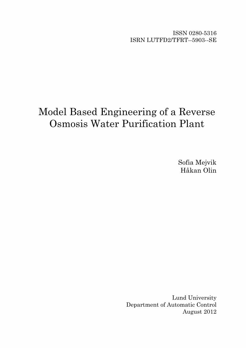
In the building block diagram, a block make up the structural backbone ofthe model. Connected to the block are a series of properties: parts, referencesand value. Parts describe the decomposition of the block into its smaller ele-ments, while references indicate that there is some sort of weaker relationshipbetween the block at hand and some other block. The value properties candescribe certain characteristics of a block, for example the component's weight.Figure 3.2 is an example of a building block diagram showing a valve repre-sented as a block and its properties. The composite association is shown asa line ending with a black diamond. Numbers next to the associations showthe multiplicities of associations. In the �gure one can see that that valve iscomposed of one handwheel but one to two packings. Also, the valve's referenceassociation with the RO-plant is shown as a line ending with a white diamond.The blocks can also contain a behavior. For example, the valve block has theoperation controlFlow().

To model a requirement, a requirement stereotype is use. The most basicrequirement stereotype consists of a string �eld describing the requirements, aswell as an ID number. When documenting the requirements for a system, oneusually start out with the most fundamental and as work progresses, new re-quirements are derived. Figure 3.3 shows a simple requirement hierarchy, withthe most fundamental requirement at the top. In order to organize the model,complex requirements are often divided into simpler once using the containmentrelationship, depicted as an line ending with a crosshair. Contained require-ments should not add any meaning to the model, but just add di�erentiation


15 August 24, 2012


Figure 3.2: Example of a block and its relationship with other blocks. Hereone can see that the valve has a composite association with a packing and ahandwheel block. The numbers next to the associations show the multiplicitiesof associations, i.e. in this case the valve contains one to two packings and onehandwheel. Also, there is a reference association with the RO-plant.

of requirements into di�erent branches. Another important relationship is thederive relationship. This is fundamentally di�erent from the containment rela-tionship. Where a containment relationship is just a di�erentiation, a derivedrelationship is based on an analysis, and is depicted as a dashed arrow with thekeyword �deriveReqt�. The arrow points at the parent requirement. To clarifythe reason for a particular design decision a rationale can be associated to eithera requirement or a relationship between requirements. To provide traceabilityin the model, one can use a satisfy relationship to assert that a model elementsatis�es a particular requirement, or a trace relationship to show the reason forthe requirement. In the �gure the valve block is said to satisfy the requirementof using a valve for �ow control.

Figure 3.3: Basic example of requirement semantics. Requirements are di�eren-tiated using the containment relationship, while new requirements are relatedto their parent requirement using the derive relationship.


16 August 24, 2012


3.5 Work�ow

In system engineering it is important to clearly state the current situation andwhat the goal is. When �rst developing the system model, the �rst thing to dois to determine the purpose and the scope of the model. The purpose of themodel could for example be to document and model an already existing systemor to specify and design a new system to be developed. When doing the later,emphasis will be more on de�ning the requirements and general system design,than on for example specifying the software implementation.

When having de�ned the purpose of the model, the next thing to consideris the scope. This is done in terms of model breadth, depth and �delity. Modelbreadth means the limits of the model, i.e. which parts that should be includedin the system and which parts should not. An example from the RO-plant couldfor example be to focus on elements involved in the puri�cation process, but forexample not include maintenance routines. Model depth on its hand meanshow detailed the model should be. Generally the model starts quite basic, justsu�cient for the basic model to be set up and as development continues, furtherdetails are added to the di�erent building blocks. To again use an examplefrom the RO-plant, one would for example start to model a valve as a blackbox controlling water �ow, but later add the type of valve and its controllerinterface. Finally, the �delity of the model means that the required level ofdetail has to be in line with purpose of the model. A low �delity diagram mightsu�ce to model the ordering of actions in an activity diagram, but not enoughfor a communication protocol [13].

As hinted above, the SysML work�ow is an iterative process, where themodel is improved gradually throughout the development process. As require-ments are gathered and use cases are created, new functional ideas may comeup, making it necessary to add new contents. Also, you may notice use casesthat are not met by any requirement. Additionally, during the structural orbehavioral development new ideas may be created forcing you to go back andchange in the model. This iterative nature of the process is illustrated as aSysML activity diagram in Figure 3.4. Finally, in the modeling stage, test casescan be created to verify that requirements are satis�ed. All of this makes themodeling a bit exhausting but when �nished a complete analysis and documen-tation of the system is done and hours and money will be saved during laterstages.

Figure 3.4: The general work�ow throughout a project, starting with the col-lection of requirements and ending with testing.

3.6 Modeling tool

In this thesis, an Eclipse based open source program called Topcased is usedto create the SysML model [15]. This program is still under development andunfortunately all of SysML's ideas are not yet supported. In Figure 3.5 a screen


17 August 24, 2012


shot from the development environment is shown. A complete documentation ofthe model can be generated but it is easier to get a good overview by browsingthe project digitally. This can be done directly in Topcased or by generating anhtml page. Topcased also contains a simulation engine to run the state machines,but in this project Matlab will be used instead, since its State�ow environmentis very well tested. At the moment Topcased is in a phase of merging withPapyrus which is a open source tool for graphical UML2 modeling.

Figure 3.5: A screen shot from the development environment in Topcased.


18 August 24, 2012

4 SysML model building


In this section the puri�cation plant will be modeled. The SysML model isbased on the approach presented in Section 3. Remember that the model de-velopment is iterative so a model step is not completely �nished when the nextstep is started. During the development of later steps you may realize that newinformation needs to be added to earlier steps. When modeling the behavior,focus will be on use case diagrams and state machine diagrams. Only someexamples of sequence diagrams and activity diagrams are introduced. In thelast part of this section some diagrams from the �nal model are presented.

4.1 Model purpose

As described in Section 3.5, the �rst thing to do when starting to model thesystem is to de�ne the purpose and scope of the model. The purpose of themodel developed in this section is to get a good documentation of the system,and give a good overview of the di�erent requirements stated by the di�erentstakeholders, with the later also de�ned. Additionally, in order to develop acontrol system, a complete description of the system components is modeled inbuilding block diagrams. Further, internal building block diagram are built todescribe the physical relation between the components.

To model the control system, several state machines are developed. Here,only the general design of the state machine will be drawn, since dynamic model-ing is better done in for example Matlab/State�ow. To show the communicationbetween the di�erent state machines, some sequence diagrams are created. Ac-tivity diagrams are also constructed to show some of the functionality sequencesused in the program.

4.2 Requirements

After de�ning the model purpose, requirements on the system were collected.The requirements were divided into �ve categories: functionality, usability, reli-ability, performance and supportability. This grouping is called FURPS and isdeveloped by Robert Grady at Hewlett-Packard [12]. This section will only showsome examples of requirement diagrams. For the full documentation, please seeAppendix A.1. The �rst category describes the functional requirements whilethe other four categories describes the non-functional requirements. The func-tional requirements describe the capabilities that the system must have. For aRO-plant the most basic capability is of course to produce clean, pure water. Toaccomplish this, the plant has to be controlled by a control system, providingthe logic for the control of the plant. The identi�ed requirements on the controlsystem are summarized in a requirement diagram in Figure 4.1. In addition tothis, due to legislation, data from the water quality has to be logged to providetraceability if the water later is discovered to have been of bad quality [16].

One important requirement that will be essential to the outline of the SysMLmodel itself and the control system is that the plant should be modular. Withmodularity, one means that parts should be easy to bring into and out of thesystem without the need to remake the whole control system or graphical in-terface. The need for modularity exists because not all of the pre�lters arepresent in every plant con�guration, for instance, as mentioned in Section 2.3.1,in Sweden the multimedia and active carbon �lter are usually omitted.

Included in the functionality group are also features that are not themselvescompletely necessary for the overall plant function, but are requirements toensure the safety and security of the plant. i.e. alarms and alerts. The most


19 August 24, 2012


Figure 4.1: Identi�ed minimum requirements on the control system. This willlater be the foundation upon which an appropriate control system is selected.

important of the two is the alarm category. An alarm is a signal that somethingfundamental is wrong with the process. A pump might have stopped workingor an essential sensor for control is no longer sending signals. The alarms willautomatically put the plant in a fail safe state, where the safety of the personnelworking with the plant is the number one priority. An alert on the other handis just a noti�cation to the operator and does not require any direct action.However, it is still an important message to the operator. An example mightbe that a pressure transmitter, not essential to the overall plant performance, isnot responding. Some alerts may also trigger an alarm after a certain amountof time if not taken care of.

The usability requirement can be seen as the customer needs. This is mainlythe requirements on the user interface. Two main requirements are an easy touse interface and four di�erent access levels. The usability requirement dia-gram can be seen in Figure 4.2. The reliability is connected to the frequencyand probability of failure. No such requirement has been stated but of coursethe failure probability and frequency should be very low. Response time, re-source usage and speed are examples of performance requirements. Since thepuri�cation plant is a very slow system speed requirements are not an issue.A resource requirement is, however, to waste as little water as possible. Fi-nally, the supportability requirements concern things such as maintainability,con�gurability, testability, compatibility, installability and portability. Some ofthe requirements in this category are for example that it should be possible tocontrol an actuator manually, to override sensor values, access data remotelyand that many other parameters should be con�gurable.


20 August 24, 2012


Figure 4.2: Requirements concerning the usability of the system, often the cos-tumer needs.


21 August 24, 2012


4.3 Stakeholders

Parallel to the requirement collection, stakeholders were identi�ed. A stake-holder is someone who has an interest in the system. This includes for examplecostumers, manufacturers and legislation. It is important to state the stake-holders in an early phase of the process since they may have requirements onthe system. If a stakeholder is forgotten it may cause serious problems whendetected. In order to �nd all stakeholders it could be a good idea to ask analready identi�ed stakeholder for other stakeholders. Identi�cation of the stake-holders of this project was performed by asking a domain expert who not onlyknew the system very well but also cooperates closely with both costumers andmanufacturers [5]. The obtained stakeholders can be seen in Figure 4.3.

Figure 4.3: Stake holders identi�ed during the modeling process.

Many of the stakeholders will have requirements outside the scope of themodel such as a stakeholder of a related system, but they are still included inthe model. The most important stakeholders to consider when later developinga control system, are the direct user of the system including an operator, main-tenance and administrative personnel. Other important stakeholders are thedevelopers of the system, both software and hardware. The software developerswill for example have an interest in a well documented software structure andan 'easy to read' code for debugging.

4.4 Building blocks

Building blocks, which were introduced in Section 3, are the parts that thesystem contain. As described in Section 2.3 a RO-puri�cation plant can bedivided into Part 1 and Part 2. Each of these blocks can then be divided intoseveral other blocks which gives a more detailed description. For example Part1 can be divided into a feed tank, a multimedia �lter, an active carbon �lterand a softening block. These blocks, in turn, can be divided into even moredetailed blocks. The lowest level described consists of valves, pumps, tanks,power supply, CEDI unit, RO unit etc. The plant parts are thus not modeledinto every screw and nut. Frequently used blocks were collected in a library thatlater was used to build blocks at a higher level. The building blocks do not showhow the blocks are connected to each other, as this is handled by the internal


22 August 24, 2012


Figure 4.4: Building block diagram showing the decomposition of the plantinto its individual modules together with the ports connected to these modules.These modules are then further modeled. As an example the control systemmodeling is shown.

building blocks described in the next section. However, to identify the buildingblocks the company's construction drawings were studied. Figure 4.4 shows abuilding block diagram where the modules of the plant are depicted. Each oneof these module blocks are linked to other building block diagrams, showing theinternal decomposition of the modules. The �gure also illustrates the buildingblock diagram for the control system. Furthermore, the �gure shows the portsconnected to each and every module. See Appendix A.4 for selected buildingblocks from the documentation.

4.5 Internal building blocks

As mention in Section 3, the internal building blocks show how the buildingblocks are connected. By combining di�erent building blocks di�erent modelsof the RO-puri�cation plant can be created. For example if the ingoing wateris of high quality all the pretreatment blocks does not have to be included.Di�erent blocks with equivalent basic functions may also be created but whenconstructing a speci�c plant model only one type is chosen. For example a valvemay have di�erent numbers of digital outputs depending on the required statusfeedback. By studying the company's construction drawings for di�erent modelsinternal building blocks diagram were created. See Figure 4.5 for an example


23 August 24, 2012


and Appendix A.5 for parts of the documentation.

Figure 4.5: Internal building block diagram showing a drawing for the RO-partholding tank. By color coding di�erent kinds of parts, one can more easilyinterpret the structure. This diagram is used to show a building block in itsphysical context.

4.6 Use cases

Use cases describe the functionality of the system in terms of user interactions.It is used to model the relationship between the system at hand, its actors anduser cases [14]. The di�erent actors acting on the system are most often takenfrom the already de�ned stakeholders. Use cases can be seen as a way to capturesystem requirements in terms of the use of the system. Therefore use casescome to include the direct users of the system, i.e. the operator, maintenancepersonnel and administrators. By asking key stakeholders, for example thesystem manufacturer or domain expert, the various use cases can be identi�ed.From these, new requirements are added to the requirement diagrams, furtherunderlining the iterative nature of the modeling process.

The most basic actor acting on the system is the observer. This is a personnot allowed to a�ect the system in any way, but only view the current statusof the plant. Important to notice is that the observer is not a stakeholder. InFigure 4.6 the observer use case diagram is depicted. The users of the systemcan be organized in a tree where the observer is the topmost parent. The childto the observer is the operator, who is the person in charge of the everydayoperation on the plant. Often this person is not quali�ed to change any plantparameters such as PID-parameters or ratios between �ows, but instead justmonitors the plant and re�lls salt and other additives when needed. As theoperator monitors the plant, reseting and checking of alarm and alerts are partof the routines. Accompanied with every change done to the system, a commentabout the reason for the changes should be included. All of this is depicted inthe �gure 4.7.

The user with the most advanced use cases is the maintenance person. Thisis the person with the most knowledge about the process itself. The maintenanceuser should have access to all the actions described in the observer and operatoruse case diagrams, as well as wide range of actions to con�gure and tune theplant. An example could be to manually open and close valves, override sensorsin order to simulate failing system components or con�gure alarm and alert


24 August 24, 2012


Figure 4.6: Use case for an observer.

Figure 4.7: Use cases for the operator. The operator inherits the use cases fromthe observer, shown in Figure 4.6.

levels. All identi�ed actions are summarized in Figure 4.8. The maintenanceuse cases are the ones that give rise to the most requirements on the controlsystem and on the human machine interface (HMI).

The administrator inherits all use cases from the maintenance user and isthe bottommost user. The detailed use case diagram can be seen in AppendixA.3.


25 August 24, 2012


Figure 4.8: Use cases for the maintenance actor. These activities give rise tomany con�guration requirements in the requirements diagrams.


26 August 24, 2012


4.7 State machines

The RO-plant has several di�erent operation modes. For example the plantcould be in production mode where the plant produce pure water or it could bein circulation mode where the plant is running but the water is not distributedto the consumers. The production mode is simply used to satisfy the consumerand give them access to puri�ed water. If the water quality becomes too pooror if the last bu�ering tank is full due to low demand of puri�ed water theproduction needs to be stopped. Still, to prevent bacteria growth, the waterthrough the membranes has to keep circulating and the plant is therefore set tocirculation mode. To model this dynamic process of producing pure water theplant was considered as a state machine where each state indicates an operationmode, see Figure 4.9.

Figure 4.9: The state machine of the plant.

Instead of an ordinary �at state machine, where all the states are on thesame level with no inner states, a hierarchical state machine is used. A statemachine consists of states that are graphically presented as a rectangular boxwith rounded corners. In each state di�erent actions can take place. The actionsare divided into entry, exit and do actions. The entry and exit actions areexecuted every time the state is entered or exited respectively, while the doactions are executed when the state is active. To transfer between di�erentstates, transitions are used. They consists of a condition, embraced by squarebrackets, that should be ful�lled. The transition could also include an actionwhich is embraced by curly brackets. To indicate the initial state a black dotis placed in the speci�c state. The state chart can also remember the history ifthe state contains a history junction, denoted as an encircled H or H*. Whena state containing a history junction is exited, the last active state is storedand the next time the state is reactivated it returns to this stored state. Usingan ordinary encircled H the history is shallow and only one level of state isremembered but by using the deep history notation with an additional * thesame state as was left is revisited, regardless of the depth of the state. Also, atransition can be split using a diamond symbol, o�ering a choice for the �naldestination state. This is just some basic information about state machines


27 August 24, 2012


but for now this knowledge is enough. In Section 5.2.2 the state machines aresimulated using the Matlab/Simulink extension State�ow and then some furtherfunctionality is presented.

Not only the entire plant can be modeled as a state machine, but also theseparate parts of the plant. For example Part 1, which consists of the feed tank,the multi-media �lter, the active carbon �lter and the softening block, can beregarded as a part with its own state machine. Part 1 can also be in productionor circulation mode since the output of Part 1 could be either closed or opened.If it is open, the part is in production mode and if it is closed the water is ledback to the feed tank and the part is in circulation mode. The state machinemodeling does not stop at this level but the feed tank, the �lters and softeningblock can in turn be regarded as individual state machines. However, theirstates do not have to be the same. For example the �lters have production anderror modes but no circulation mode. This division of the separate parts of theplant into their own state machines, further underlines the modular approachstated by the SysML model.

Figure 4.10: The state machine of the plant can be split into several statemachines which are arranged in a hierarchical way.

The state machines are also arranged in a hierarchical way, see Figure 4.10.The plant is at the top with two children, Part 1 and Part 2. Part 1 in turn hasfour children, feed tank, multi-media �lter, active carbon �lter and softeningblock. Part 2 does not have any children. It consists of the middle tank, RO,CEDI and holding tank but those parts are not modeled individually since theyare all vital parts and can not be excluded in the construction. The communi-cation between the state machines is arranged in the manner that lower levelparts report to its parent when a state change has occurred. The parent thenhandles the event and sends signals to the other parts that are a�ected by theevent. For example, if the active carbon �lter needs to do a backwash, it sendsa cleaning request to Part 1. If the cleaning procedure is possible, Part 1 sendsa cleaning con�rmation back to the active carbon �lter and appropriate signalsto the other children and the Plant.

All state machines are presented in Appendix A.10 but as an example thestate machine of Part 1, which has both a parent and children, is presentedin Figure 4.11. Even though the states may di�er somewhat, the main designfeatures are the same. All state machines consist of three outer states: ok, error


28 August 24, 2012


Figure 4.11: State machine for Part 1 which includes the feed tank, multi-media�lter, active carbon �lter and softeners.

and reset. When the ok state is active the part is ready to run, or is in someway running already. The ok state of Part 1 contains �ve inner states: standby,circulation, production, cleaning and hot water sanitization. In standby mode,the feed tank input is closed, which could also be considered as the input toPart 1, the output to Part 2 is closed and instead the valve to circulate Part 1is opened. Also all pumps are turned o�. The production state indicates thatall children are producing, the input is controlled by the level in the feed tankand the output to Part 2 is open. The same settings are used in circulationmode except that the output to Part 2 now is closed and the water is fedback to the feed tank. When the Part 1 cleaning state is active it indicatesthat some of the children are cleaning. It could either be backwashing a �lteror regenerating a softener. This state is, however, not activated when only onesoftener is regenerating since the double con�guration of softeners then switchesfrom serial to parallel mode. In this manner the production or circulation is nota�ected by a softener regeneration. During the hot water sanitization the settingare the same as for circulation but the heat exchanger is also turned on. Theerror state is simply used to indicate that something in the plant is not workingproperly. This state is activated for all parts regardless of where the actual erroroccurs. Due to the directive 2006/42/EC on machinery [17], the state machinehas to pass though a reset state before the ok state can be reentered. If theerror is handled when an reset signal occurs the process returns to the ok stateand by the deep history it returns to the speci�c inner state that was activewhen the error occurred. However, if the error is still present, the error state isreactivated.

As mentioned before the state machines will be discussed more in Section5.2.2 where the simulation is presented.


29 August 24, 2012


4.8 Activities

The actions that occurs in the state machines can be further modeled by theusage of activity diagrams. In an activity diagram the initial start point is, asin the state machine diagram, shown as a black dot. The activity is presentedin a box and transitions between parts are show by arrows. Other parts thatare frequently used in activity diagrams are the fork node and join node. Theseare illustrated as bars and as the names indicate, the fork node splits the �owwhile the join node combines it. Those nodes can be used to synchronize the�ow. The merge node and decision node also combine and split �ows but lackthe synchronization. A dashed region with a hourglass indicates that the regionmight be interrupted. To show that an activity has come to an end the exitpoint is used. It is illustrated as a black dot encircled with an extra circle. Anexample is presented in Figure 4.12 where the production state of Part 1 is justentered. The output valve to Part 2 is opened and the recirculation valve inPart 1 is closed. In more detail this can also be modeled as in Figure 4.13. Herethe response times for the valves are limited and depending on the reply theactivity diagram reports di�erent outcomes. The last activity diagram is a bitmore detailed but for the modeling purpose the �rst is enough.

Figure 4.12: This activity diagram shows the actions that occur when the pro-duction state of Part 1 is entered.

Figure 4.13: In this activity diagram the outcome of the activities are takeninto consideration. If the valves limited response time expires or if the reply isnot as expected the activity takes an alternative exit path.


30 August 24, 2012


As the activity diagram is well suited to model functionality sequences, thesequence for cleaning is shown in Figure 4.14. When performing a cleaning thefollowing sequence is executed:

1. Fill holding tank

2. Backwash

3. Afterwash

4. Reset

Some more examples of activity diagrams can be seen in Appendix A.8.

Figure 4.14: Activity diagram illustrating the cleaning sequence of the activecarbon �lter.

4.9 Sequence diagram

A sequence diagram shows how di�erent parts in the system interact over time.Figure 4.15 illustrates the sequence of the communication, when the power isturned on. Each part has a timeline and the communication between the partsis presented by arrows. A call is a solid line while a reply is dashed.

More sequence diagrams are shown in Section 6.4 and in Appendix A.9.


31 August 24, 2012


Figure 4.15: A sequence diagram showing the communication between the sys-tem parts when the system is powered on.

4.10 Final model

As mentioned before, the modeling procedure is an iterative process, where newcontent is added as the project proceeds. Initial basic diagrams are continuouslyupdated until they reach the desired depth of the model. To show this, Figure4.16 shows the �nal version of Figure 4.2, where the reason for the di�erentrequirements are added. As many of the usability requirements originate fromuse cases, most of the requirements are also traced back to these use cases. Butthe trace relationship only shows the reason for the requirement. To show thata requirement has been meet, the satisfy relationship is used. In the �gure, thewhole login requirement is said to be satis�ed by the control system.

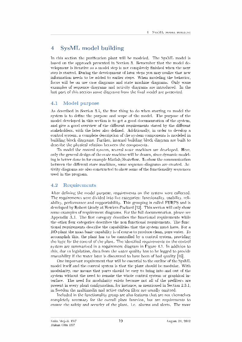
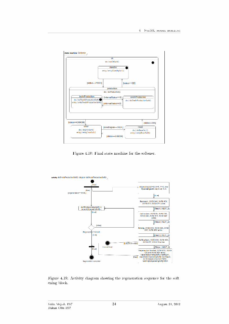
Diagrams modeling the intended dynamic behavior of the plant are especiallyprone to be changed as the project progresses. Often, the �rst idea of howthe software should communicate or how a synchronization phase should beperformed has to be redesigned during the implementation phase. Still the �rstideas are used as a foundation for the continued development. Figure 4.17 and4.18 show the initial and �nal state machine for the softener. For example onesees that the hierarchical approach was not initially considered and that thereset state was not included. Also, to illustrate the functionality sequence, anactivity diagram was added in the �nal version, instead of creating states foreach function, see Figure 4.19.


32 August 24, 2012


Figure 4.16: Updated version of Figure 4.2, where the reason for the particularrequirements are depicted by the trace relationship. Also, the whole interfacerequirement is satis�ed by the control system.

Figure 4.17: Initial state machine for the softener.


33 August 24, 2012


Figure 4.18: Final state machine for the softener.

Figure 4.19: Activity diagram showing the regeneration sequence for the soft-ening block.


34 August 24, 2012

5 Modeling and simulations


First a mathematical model for the RO part was derived. The model was thentransfered to Matlab/Simulink and simulated and control strategies were devel-oped. The state machines developed in the SysML model were also implementedin Matlab/Simulink using State�ow.

5.1 Mathematical model of the reverse osmosis process

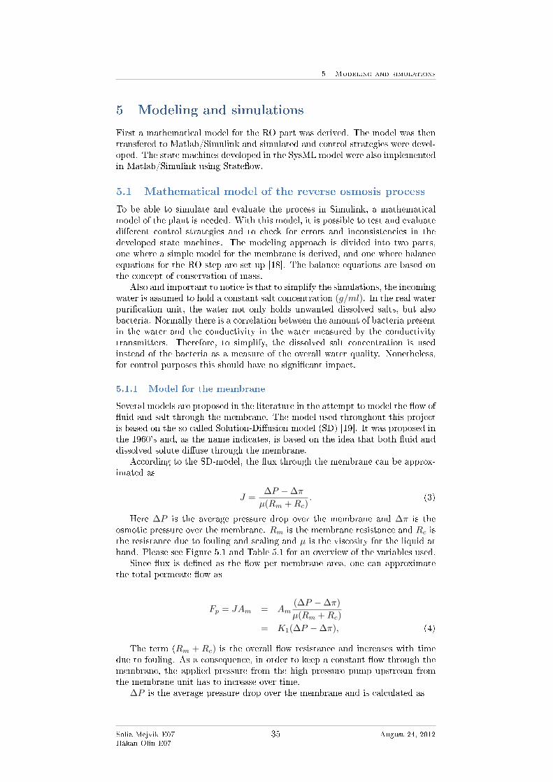
To be able to simulate and evaluate the process in Simulink, a mathematicalmodel of the plant is needed. With this model, it is possible to test and evaluatedi�erent control strategies and to check for errors and inconsistencies in thedeveloped state machines. The modeling approach is divided into two parts,one where a simple model for the membrane is derived, and one where balanceequations for the RO-step are set up [18]. The balance equations are based onthe concept of conservation of mass.

Also and important to notice is that to simplify the simulations, the incomingwater is assumed to hold a constant salt concentration (g/ml). In the real waterpuri�cation unit, the water not only holds unwanted dissolved salts, but alsobacteria. Normally there is a correlation between the amount of bacteria presentin the water and the conductivity in the water measured by the conductivitytransmitters. Therefore, to simplify, the dissolved salt concentration is usedinstead of the bacteria as a measure of the overall water quality. Nonetheless,for control purposes this should have no signi�cant impact.

5.1.1 Model for the membrane

Several models are proposed in the literature in the attempt to model the �ow of�uid and salt through the membrane. The model used throughout this projectis based on the so called Solution-Di�usion model (SD) [19]. It was proposed inthe 1960's and, as the name indicates, is based on the idea that both �uid anddissolved solute di�use through the membrane.

According to the SD-model, the �ux through the membrane can be approx-imated as

J =∆P −∆π

µ(Rm +Rc). (3)

Here ∆P is the average pressure drop over the membrane and ∆π is theosmotic pressure over the membrane. Rm is the membrane resistance and Rc isthe resistance due to fouling and scaling and µ is the viscosity for the liquid athand. Please see Figure 5.1 and Table 5.1 for an overview of the variables used.

Since �ux is de�ned as the �ow per membrane area, one can approximatethe total permeate �ow as

Fp = JAm = Am(∆P −∆π)

µ(Rm +Rc)

= K1(∆P −∆π), (4)

The term (Rm + Rc) is the overall �ow resistance and increases with timedue to fouling. As a consequence, in order to keep a constant �ow through themembrane, the applied pressure from the high pressure pump upstream fromthe membrane unit has to increase over time.

∆P is the average pressure drop over the membrane and is calculated as


35 August 24, 2012


∆P =Pf + Pr

2− Pp, (5)

where Pf , Pr and Pp is the pressure on the feed side, retentate side andpermeate side respectively.

∆π is the osmotic pressure over the membrane

∆π = iRT (Ct − Cp)

= K2(Ct − Cp). (6)

where T is the temperature and R is the gas constant. i is the van't Ho�factor and is approximated to two. In our case we will also consider the tem-perature T as constant at 25 degrees Celsius or 298 Kelvin.

The salt �ux through the membrane can be written as

Cp = K3Ct, (7)

where K3 is a constant describing how much salt that goes through themembrane. K3 usually lies between 0.01 and 0.001. In our case, a membraneLE-4040 from Dow Filmtec

TM

is used, which according to datasheets has a saltrejection of 99 %, i.e K3 can be assumed to be 0.01.

5.1.2 Modeling the RO-block

Figure 5.1: Schematic diagram of the reverse osmosis block.

In order to minimize the water going to waste, balance equations have tobe set up in order to evaluate the system and controller performance. First thevolume balance is set up, where the change in total volume, dVtot

dt , is equal tothe di�erent �ows coming in and out of the system

dVtotdt

= Fin − Fp − Fd. (8)

In order to minimize the water going to waste during circulation, a balanceequation for the total salt amount in the system has to be set up

VtotdCt

dt= FinCin − FpCp − FdCt. (9)

where Fin and Cin are design parameters. This can then be rearranged as

dCt

dt=FinCin − FpCp − FdCt.

Vtot. (10)


36 August 24, 2012


Table 5.1: Variables used in the reverse osmosis modeling

Parameter DescriptionAm Total membrane areaCin Salt concentration for incoming waterCp Permeate concentrationCt Concentration in the tankFin Incoming �ow from Part 1Fd Retentate �ow to drainFp Permeate �owi Van 't Ho� factorJ Membrane �uxK1 Variable used in equation 4K2 Constant used in equation 6K3 Constant used in equation 7Pf Pressure on the membrane feed sidePp Pressure on the permeate sidePr Pressure on the retentate sideR Gas constantT Temperature in KelvinRm Membrane resistanceRc Membrane resistance due to foulingµ ViscosityVtot Estimated volume for the whole system∆P Mean pressure di�erence over the membrane∆π Osmotic pressure di�erence over the membrane

5.2 Simulink simulation

From the simple model for the membrane and the balance equations describedabove in Section 5.1, a dynamic model for the system is setup in Simulink,see Figure 5.2. By connecting a simple control system to these equations, itis possible to evaluate di�erent approaches for controlling the plant. The �nalobjective is to control a total of four variables in Part 2, see Figure 5.3. Theobjectives for the four control loops are listed below.

• Water tank levels. The water levels in the tanks, i.e. the middle tank andthe holding tank, should be controlled thereby guaranteeing that therealways is enough water in the system.

• Permeate �ow. The permeate �ow should be kept constant over time.This is done by controlling the high pressure pump in front of the RO-membranes. In the already existing control system, a pressure transmitterin front of the membranes is used to ensure that the pump output gives riseto a high enough pressure right in front of the membranes. Due to fouling,the term Rc in equation 4 will increase. In order to be able to keep thepermeate �ow constant it is not enough to just keep the input pressureconstant, one also has to compensate for this increasing resistance byincreasing the pressure from the pump. In order to do that, the permeate�ow has to be measured, either directly with a �ow indicator, or indirectlywith pressure transmitters.

• Retentate �ow to drain. The fourth and last control loop is the conductiv-ity feedback from the permeate side to the retentate drain. This is donein order to be able to control the amount of retentate let to drain.


37 August 24, 2012


Figure 5.2: Balance equations setup in Simulink to evaluate the di�erent con-troller approaches. At the top one can see the membrane equation. In themiddle the balance equation for the water in the system is shown and at thebottom the equation for the total salt concentration is shown.

Figure 5.3: Figure showing the RO-unit and the four control loops involved.

5.2.1 Control approach

The simplest possible controller is the on/o� controller, where one simply justswitch between two modes depending on the control error. The valves control-ling the �ow into the two tanks are binary valves, and this gives no other option


38 August 24, 2012


but to use a on/o� control approach for controlling the level in the tanks. Thewater level could be controlled in a PWM manner, but this would rapidly wearthe valves out. Instead, the water levels will be allowed to �uctuate betweentwo predetermined levels, say levelmin and levelmax.

As mentioned above in Section 5.2, the fouling of the membrane requires thehigh pressure pump to increase its output pressure with time. As this foulingand scaling process is a very slow process, the �rst approach taken is to evaluatethe use of a simple PID-controller for ramping up the reference pressure. Thecontroller is implemented as a simple Simulink block with appropriate inputsand outputs, see Figure 5.4. A thing to keep in mind is that the membraneshave a maximum allowed pressure limit. If exceeding this pressure, there is arisk of pushing the membranes out of their containers, an issue called telescopingin membrane terminology [20]. When the pressure exceeds this limit, the plantshould automatically shut down in wait for the membranes to either be cleanedor replaced. To prevent this a saturation block is added to the control signaloutput.

In the simulation the permeate �ow is directly measured with a �ow trans-mitter which is fed back to the control system. In the simulation scenario, thetotal membrane resistance is assumed to increase with 50 % over the course ofone month. Figure 5.5 shows the behavior of the �ow both without and withthe �ow feedback. Obviously, as seen in the topmost plot, without the �owfeedback, the pressure from the pump will remain constant and the �ow willdecrease over time. The bottom �gure shows the same �ow but with the con-trolled pressure. Not surprisingly, a PID-controller seems to cope well with theslow dynamics of the process.

Figure 5.4: Simulink representation of the PID-controller.

Out of the four control objectives, the most complicated is the conductivityfeedback from the permeate side. Depending on the size of the tank and theoverall water amount left in the piping, the time constant for the process canbe quite big, giving rise to a slow step response. On the other hand, the waterconductivity will most certainly not make any sudden changes, and hopefullythis time constant will not give rise to any serious problems. Another PID-controller, with the same design outline as in the pressure feedback control loopshown in Figure 5.4, is used as controller.

In the simulations, the output signal from the controller is a ratio expressedin percentage, determining how much of the water that should be fed back tothe holding tank, and how much should be allowed to go to drain. In this PID,there are some constraints that have to be included. One is that the controlsignal can not be allowed to be greater than 1, i.e 100 %, since one can notlet more water to drain than physically possible. Actually, the portion let todrain would normally not exceed 10 % of the retentate �ow. Another importantthing is to add an anti-windup constraint to the I-part in the controller. Theslow dynamics of the system together with the constraint on the control signalcould otherwise lead to problems during big reference changes. The anti windup


39 August 24, 2012


Figure 5.5: Di�erence between the uncontrolled and controlled permeate �ow.Upper �gure shows the decline of permeate �ow with a membrane resistanceincreasing with 50 % over a course of one month. The bottom �gure shows thesame scenario but with the PID plugged in. The reference �ow is set to 0.00013m3/s or approximately 500 l/h

is simply implemented as a upper saturation limit in the integrator block ofthe controller. In Figure 5.6 three negative step responses are shown for theRO-process. During theses simulations an input water with a concentration of0.5kg/m3 is used, which corresponds to the salt concentration of drinking water.From the �gure, one see that the permeate concentration slowly drops towardsthe new reference. Due to the constraints on the drain �ow, the concentrationdrops fairly slow towards the new value. Tuning the PID-controller will notimprove the performance as the control signal is saturated during the decline.The bottommost �gure shows the response when the reference changes to anunreachable value of 4g/m3. As the membrane has a salt rejection of 99 %, onecan only expect to reach a permeate concentration of 5g/m3.

One thing to keep in mind is that the simulations done is just a way totest di�erent controller approaches and validate their performance. The controlparameters used in the simulations can not be used on the real process due to themany assumptions done. Also, as the real process comes in many di�erent sizes,the dynamics of the system will vary from model to model. This is shown inFigure 5.7. By increasing the total water volume in the system, the response to achange in reference concentration takes longer. The corresponding �ow ratios forthe step responses in Figure 5.7 is shown in Figure 5.8. In the �gure, the drain�ow makes a step to zero as the salt concentration reference changes at t=500.By not letting any salt go to drain on the retentate side, the concentrationquickly increases in the system. When the salt concentration reaches the desiredreference, the drain �ow stabilizes around 30 %, i.e. 30 % of the retentate islet to drain, while the rest is fed back to the bu�er tank. To �nd controllerparameters for a real plant, methods such as the Ziegler-Nichols method couldbe used.

To conclude the control approach section, PID-controllers seem to be able


40 August 24, 2012


Figure 5.6: Figure showing three inverted step responses when changing thepermeate concentration reference in the RO-process. The simulations are donewith an input water with a salt concentration of 0.5kg/m3, corresponding tonormal drinking water. Due to the constraints on the drain �ow, the concentra-tion drops slowly towards the new reference. In the bottom �gure the referencetakes a step to a reference not possible to reach.

Figure 5.7: By increasing the total water volume in the system, one gets a slowerresponse to a concentration reference change.

to handle both the upramping of pressure over the membrane as well as theconductivity feedback.


41 August 24, 2012


Figure 5.8: Ratio of �ows ( flowdrain

flowretentate) for the step responses shown in Figure

5.7. As the salt reference change at t=500, the drain valve closes, and allretentate is fed back to the bu�ertank. As the salt concentration reaches thereference, the �ow to drain stabilizes around 30 % of the total retentate �ow.

5.2.2 State machine

In this section simulations of the state machines that were modeled in Section 4.7are performed. In order to simulate the dynamic behavior, the Matlab/Simulinkextension State�ow is used. Later in Section 6 those state machines are imple-mented in C code.

The syntax to model a state machine in State�ow is similar to what waspresented in Section 4.7, however, some small changes exist and in order torun the state machines it is important that the syntax is correct. As describedearlier, di�erent actions types take place in a state. It could for example be anentry action or a exit action. In State�ow, those keywords are the same butthe do-action is instead called during. Also to perform the transitions correctly,the syntax of the transition action type is important. State�ow uses the fol-lowing syntax: event_trigger[condition]{condition_action}\transition_action.The event_trigger is the event that triggers the transition. Additionally, theevent_trigger may have a condition and/or a condition action. If an event istriggered and the condition is ful�lled the condition action is executed. Finallythe transition can also have a transition action that is executed when the transi-tion occurs. Instead of a black dot in the initial state, State�ow uses a black dotwith an arrow pointing at the initial state. The history junction is representedlike described in Section 4.7, but the ordinary junction symbol is instead of thediamond represented as a circle. In State�ow, Matlab function blocks can alsobe added where ordinary Matlab code can be implemented. As mentioned be-fore this is just the basic of state machines and State�ow has a lot more to o�er.For example states can be executed simultaneously and then the circumferenceon the rectangle shaped state is dotted instead of a solid line. However, thepresented information is enough in order to grasp the state machines in thisthesis.

The state machine of Part 1 is once more presented, in Figure 5.9, but now


42 August 24, 2012


the implementation from State�ow is shown. Unfortunately transitions couldnot handle enumerators so instead of the state names a number is used. Thefollowing table gives the translation between numbers and state names used inthe state machine of Part 1 :

Number Abbreviated state name Formal state name0 SB Standby1 PROD Production2 CIRC Circulation3 ERROR Error4 CLEAN Cleaning5 SAN Hot water sanitization-2 ERROR Error (Only used in Matlab)-3 OK Ok

Table 5.2: Table for mapping the status number used in Matlab to the enumer-ator used in SysML.

The complete translation table is found in Appendix B together with allstate machines implemented in Matlab. One particular thing to notice in theState�ow diagrams is the additional status signal, -2, which is used to return tothe error state from the reset state. This is needed since the State�ow imple-mentation does not store events in queues but instead continuously reads thestatus ports. Another status signal used but not mentioned in the table is -1.This signal is used to synchronize the transitions from the reset state. Beforethe -3 signal is sent, all of the children have to send -1 to its parent indicat-ing that no error exists in them. When the plant receives -1 from both Part1 and Part 2, a -3 signal is sent back down, stating that it is ok to return toproduction. Likewise, Part 1 sending -1 means that it received -1 from all ofits children. This reset function is also implemented on the PLC and will befurther discussed in section 6.4 where a sequence diagram diagram of the resetsynchronization procedure is presented.

The di�erent StateFlow state machines are then encapsulated in a Simulinkstate chart block which in turn is connected to its children's state chart blocks.Part 1 and its children can be seen in Figure 5.10. On a higher level this blockis connected to the state machine of the plant. Those connections, includingthe connection to Part 2 is also presented in Appendix B.


43 August 24, 2012


Figure 5.9: Part1 state machine implemented in State�ow.


44 August 24, 2012


Figure 5.10: Simulink model of Part1 and its children, the feed tank, the mul-timedia �lter, the active carbon �lter and the softeners.


45 August 24, 2012

6 Implementation

6 Implementation

This section covers the implementation on the PLC. First, the system choice isbrie�y discussed and some general information about the functionality of thePLC. Later the structure of the program is described. Both the state machinesand the mathematical model simulated in Simulink are transfered to C codeand implemented on the PLC.

6.1 System choice

From the requirements diagrams in the SysML model, one can see a couple ofrequirements concerning the choice of control system. Some of them are listedbelow:

• Number of I/Os. The system should be able to handle the required numberof input and output ports. For the RO-plant, this varies from model tomodel, but a minimum of 60 inputs and 60 outputs are required.

• Communication protocols. The communication with actuators should bedone via a �eldbus. Also it should support TCP/IP to support remotereading of data from the HMI.

• Modularity. It should be easy to add and remove modules from the system.

• Programming language. The system should support the programminglanguages de�ned by IEC 61131-3, but also C.

Although there may be several systems that ful�ll these requirements, thecontrol system choice fell on the X20CP1485-1 system from B&R. The X20supports a total of 250 I/O modules or 3000 channels. Further it supportsEthernet TCP/IP and has a 64 MB DRAM and 1 MB SRAM internal memory[21] . All of this is well enough for the needs of the RO-plant. Also the PLCs fromB&R come with their own development environment called B&R AutomationStudio. Automation Studio supports development in the languages stated byIEC 61131-3 and C but also C++ with a special package. After the choice ofsystem is done, the SysML model is updated with the appropriate relationship,see Figure 6.1.


46 August 24, 2012

6 Implementation

Figure 6.1: Requirement diagram concerning the control system, with the B&RX20 system added to underline that it satis�es the requirements.

6.2 PLC

A programmable logic controller, or PLC, is a low cost computer often used inautomation industry. The development of the PLC started in the 60's from thedesire to replace old analog controllers with digital ones [22]. It consist of themain logic controller and a number of attached inputs and outputs, as well assome communication interface, see Figure 6.2.

Figure 6.2: The PLC execution cycle consists of three steps. First, the mappingof input signals, followed by the program execution and the mapping to outputs.

When switched on, the PLC executes its programs in a cyclic manner, witheach program executed exactly once each cycle [23]. During the start of eachcycle, the input ports are scanned and values are transfered to an I/O imagetable, where every input value is mapped to a software variable in the PLC.


47 August 24, 2012

6 Implementation

After the scanning, the programs are executed in a predetermined order, somemore often than others depending on their priority. When every program hasexecuted, any changed variable is mapped to their corresponding output port.Figure 6.3 shows a priority table from Automation Studio where two tasks,LogActivity and RO_sim are assigned to execute every 50 ms and PLANTSMwhich is assigned to execute every 200 ms. Figure 6.4 shows how the tasks willexecute during runtime. If LogActivity and RO_sim �nish their cyclic tasksin 10 ms and 5 ms respectively, there will be 35 ms of idle time during each50 ms cycle, leaving room for PLANTSM to execute. If any task fails to �nishduring its assigned cyclic time, a cycle time violation error will be thrown andthe system will enter service mode if not handled.

Figure 6.3: Di�erent cyclic tasks can be assign to execute more or less often,depending on their priority. The �gure shows the priority assignment table fromB&R Automation Studio.

Figure 6.4: Execution order for the 50 ms cyclic tasks LogActivity and RO_sim.Any idle time during the 50 ms cycle can be used to execute the PLANTSMtask.

6.3 Libraries

To keep the modular approach, de�ned as a requirement in the SysML model,the programming task is divided into several libraries, one for each of the phys-ical modules in the plant. Starting out from the simplest components in theplant, i.e. valves and sensors, more and more advanced and complex functionsare created. The valve library will for example contain functions to open andclose a speci�c valve, check if the valve is open/closed etc, see below.

. . .p l c b i t va lveClose ( s t r u c t Valve ∗pValve ){

i f ( pValve==0){re turn FALSE; // nu l l p o i n t e r}pValve−>output=FALSE; //Close va lvere turn TRUE;

}. . .

The feed tank library in its turn, see below, will contain functions to setthe tank in its di�erent operation states, using the functions previously de�ned


48 August 24, 2012

6 Implementation

in the valve library. The feed tank library also contains di�erent functions forchecking possible alarms. Additionally, get and set operations for speci�c sensorreadings and alarm levels are implemented.

. . .p l c b i t setStandbyModeFeed ( FeedTankBlock ∗pFeedBlock ){

i f ( pFeedBlock==0){re turn FALSE; // nu l l p o i n t e r

}setOperat ionStateFeed ( pFeedBlock , STANDBY_S) ;va lveClose (&pFeedBlock−>feedTank . inputValve ) ; //CLOSE XV30−02pumpStop(&pFeedBlock−>PU30_01 ) ; //STOP PU30−01pumpStop(&pFeedBlock−>PU30_02 ) ; //STOP PU30−02re turn TRUE; //Function OK

}. . .

6.4 Hierarchal state machine

The most common way to implement a state machine is to use a �at statemachine, where all the states are on the same level and with no inner states.This is easily implemented in code using a switch case statement. An exampleconsisting of three states can be seen in the code below and the arrangement ofstates is depicted in Figure 6.5.

Figure 6.5: Example state machine described in code below.

State myState ;

void myStateHandler ( unsigned const s i g n a l ){switch (myState ){ // Switch on the cur rent s t a t ecase STANDBY:

switch ( s i g n a l ){ // Switch on incoming s i g n a lcase ERROR_S:

myState=ERROR; //Change s t a t ebreak ;

case PRODUCTION_S:myState=PRODUCTION; //Change s t a t ebreak ;

}break ;

case PRODUCTION:switch ( s i g n a l ){ // Switch on incoming s i g n a lcase ERROR_S:


49 August 24, 2012

6 Implementation

myState=ERROR; //Change s t a t ebreak ;

case STANDBY_S:myState=STANDBY; //Change s t a t ebreak ;

}break ;

case ERROR:switch ( s i g n a l ){ // Switch on incoming s i g n a lcase STANDBY_S:

myState=STANDBY; //Change s t a t ebreak ;

case PRODUCTION_S:myState=PRODUCTION; //Change s t a t ebreak ;

}break ;

}}

This very simple way of implementing a state machine has both its pros andcons. The advantages are that it is simple, one do not have to be a professionalprogrammer to understand what it does and its memory footprint is small asone only needs an enumerator to represent each state. The disadvantages arethat the construction does not have any built in support for either entry or exitconditions nor for nested states. Manually coding the entry/exit behavior willsoon lead to a hard to read code. Entry behavior to a state will for example bespread out in every state that can make a transition to the state in question [24].

Instead of �at state machines the idea of hierarchical state machines, whichconsists of nested states, was used. This reduces the transitions since the par-ent's transitions only have to be declared once and not in all of the inner states.The hierarchical state machine implementation in this thesis is based on theapproach by Miro Samek, and a framework called Quantum Leaps [25]. Quan-tum Leaps uses, in short, instead of long switch/case statements, functions andfunction pointers to organize the state machines. This framework also containsbuilt in support for entry and exit conditions. The principle is perhaps bestillustrated with a code example, with the same three states as before.

. . .

QState STANDBY( feedTank_S ∗me, QEvent const ∗e ) {switch ( e−>s i g n a l ) { // Switch on incoming s i g n a l s

case Q_ENTRY_SIG: { //Do entry ac t i onre turn Q_HANDLED( ) ;

}case Q_EXIT_SIG: { //Do ex i t ac t i onre turn Q_HANDLED( ) ;

}case PRODUCTION_S: {re turn Q_TRAN(&PRODUCTION) ; //Make t r a n s i t i o n to PRODUCTION

}case ERROR_S: {re turn Q_TRAN(&ERROR) ; //Make t r a n s i t i o n to ERROR

}case DURING_S: {

doStandbyStuff ( ) ; //Perform during ac t i onre turn Q_SUPER(&QHsm_top ) ; //Pass event to parent s t a t e machine

}}

re turn Q_SUPER(&QHsm_top ) ; // No match , pass event to pseudo SM.}


50 August 24, 2012

6 Implementation

QState PRODUCTION( feedTank_S ∗me, QEvent const ∗e ) {switch ( e−>s i g n a l ) { // Switch on incoming s i g n a l s

case Q_ENTRY_SIG: { //Do entry ac t i onre turn Q_HANDLED( ) ;}case Q_EXIT_SIG: { //Do ex i t ac t i onre turn Q_HANDLED( ) ;}case STANDBY_S: { //Make t r a n s i t i o n to STANDBYreturn Q_TRAN(&STANDBY) ;}case ERROR_S: { //Make t r a n s i t i o n to ERRORreturn Q_TRAN(&ERROR) ;}case DURING_S: {

doProduct ionStuf f ( ) ; //Perform during ac t i onre turn Q_SUPER(&QHsm_top ) ; //Pass event to parent s t a t e machine}

}re turn Q_SUPER(&QHsm_top ) ; // No match , pass event to pseudo SM.}

QState ERROR( feedTank_S ∗me, QEvent const ∗e ) {switch ( e−>s i g n a l ) { // Switch on incoming s i g n a l s

case Q_ENTRY_SIG: {// Do entry ac t i onre turn Q_HANDLED( ) ;}case Q_EXIT_SIG: {// Do ex i t ac t i onre turn Q_HANDLED( ) ;}case STANDBY_S: { //Make t r a n s i t i o n to STANDBYreturn Q_TRAN(&STANDBY) ;}case PRODUCTION_S: { //Make t r a n s i t i o n to PRODUCTIONreturn Q_TRAN(&PRODUCTION) ;}case DURING_S: {

doErrorStu f f ( ) ; //Perform during ac t i onre turn Q_SUPER(&QHsm_top ) ; //Pass event to parent s t a t e machine}

}re turn Q_SUPER(&QHsm_top ) ; // No match , pass event to pseudo SM.}. . .

The code might be hard to understand at �rst, but once you understand themechanism behind it, the construction of the state machine is simpli�ed a lot. Inthe framework, there are three reserved events, Q_ENTRY_SIG, Q_EXIT_SIG andQ_INIT_SIG. The �rst two signals are generated by the framework itself, oncea state is either entered or exited. The init-event is used to specify where in ahierarchy of states that the state machine should start. In the example there areno nested state, so this signal is not used. Apart from these three enumerators,the developer is free to de�ne his or hers own signals. In the example, theuser-de�ned signals are STANDBY_S, PRODUCTION_S and ERROR_S. Once a signalis generated somewhere in the system, it is sent to a dispatch functions thattraverses the state machine and checks if the current innermost active state hasany valid transition to pair with the signal. If it does, the transition takes placeand the corresponding exit and entry actions are performed and the event issaid to be handled. If there is no valid transition, the signal is passed to theclosest parent of the current state, as the parent might have a valid transition inresponse to the event. If no state in the current active state hierarchy handlesthe event, it is passed to a pseudo state, QHsm_top which is the topmost state ofthe state machine, where the event is automatically handled without any action.


51 August 24, 2012

6 Implementation

The Quantum-Leap framework has, however, no built in support for a during-behavior, and to solve this, a DURING_S signal was created. This signal is gener-ated when no other user-de�ned event takes place. The DURING_S signal is sentto the innermost active state and then passed upwards in the state hierarchy asevery active state should perform the during action. The deep history junctionis implemented by introducing a state variable and saving the active state everytime a nested state is entered. When reseting from an error, the state machinewill then return to the state referenced by the state variable.

As mentioned before the PLC runs in a cyclic manner, performing one taskafter another. There exists one task for each state machine, but also one cyclictask that handles the graphical user interface (GUI). The execution order islisted below:

1. GUI

2. Plant

3. Part 1

4. Part 2

5. Feed tank

6. Multimedia �lter

7. Active carbon �lter

8. Softening block

Since the GUI only communicates with the Plant state machine, a signal fromthe GUI is handled during the same cycle as it was sent. An error signal fromthe feed tank, however, takes one cycle to reach Part 1 and another one toreach the Plant. Since the cycle times are quite short, the delay from child toparent is not a problem. During development the time for each cycle has been1 second but this is a design parameter that can be changed. The chosen timewas appropriate during real-time debugging.

To handle the sending of event in the state machine, a number of event-queues are used, one for every individual state machine. The queues are neededin order to be able to handle numerous events being sent during the sameexecution cycle. This may only happen on very rare occasions on the real processas the cycle time will be quite small, but it does still need to be handled.

During each execution cycle, every state machine starts by checking for anyerrors within itself. If an error is detected, an alarm is generated and an eventERROR_S is generated. This event sets the whole plant in a fail safe state.However, if no error is detected, the program continuous and checks for anyincoming events in its corresponding event queue. If any events are presentin the queue, they are sent to an event handler that provides the logic forthe communication between the state machines. The procedure is shown in asequence diagram in Figure 6.6. In the �gure, if the feed tank detects an error,it puts itself in a fail safe state and sends an ERROR_S event to the Part 1 statemachine, which in turn, puts itself in a safe mode while passing the messageupwards to the Plant and down to its other children.

Reseting the plant from an error requires some synchronization between thedi�erent state machines. When the operator sends a reset signal from the GUI,the signal, RESET_S, is sent to the topmost state machine, which in turn dis-tributes the signal. Figure 6.7 shows a SysML sequence diagram, describing thesynchronization process. The execution order of the individual state machinesdetermines the number of cycles it takes for the whole plant to reset. It takes


52 August 24, 2012

6 Implementation

Figure 6.6: Sequence diagram illustrating the procedure during one task cycle.First, the state machine checks for errors. If any, an ERROR_S event is dispatched,putting the state machine in a fail safe mode. The ERROR_S event is then passedon to the parent state machine. If no errors are detected. the event queue ischecked for incoming events. If any, the appropriate action is taken by an eventhandler. Last the status of the state machine is updated. When the Part1 taskexecutes, it will handle the event from the Feed tank and pass it along to thePlant.

one cycle to tell all state machines to make a transition to their reset states.Once there, the individual parts will send a reset request to their parent. Theparent will in turn ask the Plant if it is in order for the sub state machines to re-turn to operation. If so, an OK_S signal is dispatched and operation is resumed.All of the signals used in the state machines can be seen in Appendix C.


53 August 24, 2012

6 Implementation

Figure 6.7: SysML sequence diagram illustrating the reset synchronization pro-cedure when reseting from an error.


54 August 24, 2012

6 Implementation

To show and debug the execution of the state machine, logging functionsfor the state machines were implemented. At the start of every cycle, the mainlogger writes the current cycle number, as well as the current status for everyindividual state machine to a �le. Also individual loggers are created for each ofthe state machines. In these loggers more information about the transitions arelogged. However, to get a better overview, only comments from those logs areposted in the example of the main logger below. The example shows the stateof events that take place when the multi-media �lter wants to do a backwash.

Cycle # State Machine Current State CommentCycle 48:

Plant: PRODPart1: PRODPart2: PRODFeed: FILLMM: PROD //Multimedia �lter wants to clean.

//Sends CLEANING_S to Part 1AC: PRODSoft: PROD

Cycle 49:Plant: PRODPart1: CLEAN //Enters clean mode. Sends CLEANING_S

//back to MM, and STANDBY_S to AC// and Soft. Sends CIRCULATION_S to Plant

Part2: PRODFeed: NOFILLMM: CLEAN // Multimedia enters cleaning modeAC: SB // Enters standby modeSoft: SB // Enters standby mode

Cycle 50:Plant: CIRC // Enters circulation modePart1: CLEANPart2: PRODFeed: NOFILLMM: CLEANAC: SBSoft: SB

......

......

......Cycle 56:

Plant: CIRCPart1: CLEANPart2: PRODFeed: NOFILLMM: CLEANAC: SBSoft: SB

Cycle 57:Plant: CIRCPart1: CLEANPart2: PRODFeed: NOFILLMM: PROD //Done cleaning. Sends DONE_CLEANING_S

//to Part 1


55 August 24, 2012

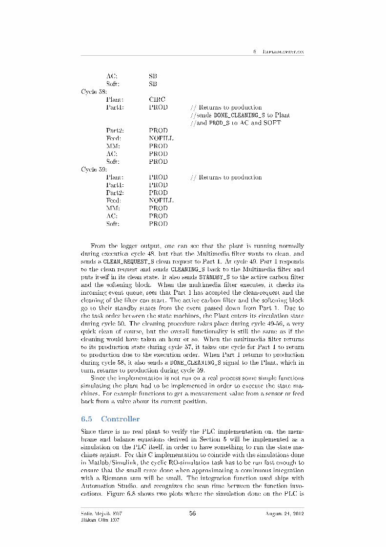
6 Implementation

AC: SBSoft: SB

Cycle 58:Plant: CIRCPart1: PROD // Returns to production

//sends DONE_CLEANING_S to Plant//and PROD_S to AC and SOFT

Part2: PRODFeed: NOFILLMM: PRODAC: PRODSoft: PROD

Cycle 59:Plant: PROD // Returns to productionPart1: PRODPart2: PRODFeed: NOFILLMM: PRODAC: PRODSoft: PROD

From the logger output, one can see that the plant is running normallyduring execution cycle 48, but that the Multimedia �lter wants to clean, andsends a CLEAN_REQUEST_S clean-request to Part 1. At cycle 49, Part 1 respondsto the clean-request and sends CLEANING_S back to the Multimedia �lter andputs itself in its clean state. It also sends STANDBY_S to the active carbon �lterand the softening block. When the multimedia �lter executes, it checks itsincoming event queue, sees that Part 1 has accepted the clean-request and thecleaning of the �lter can start. The active carbon �lter and the softening blockgo to their standby states from the event passed down from Part 1. Due tothe task order between the state machines, the Plant enters its circulation stateduring cycle 50. The cleaning procedure takes place during cycle 49-56, a veryquick clean of course, but the overall functionality is still the same as if thecleaning would have taken an hour or so. When the multimedia �lter returnsto its production state during cycle 57, it takes one cycle for Part 1 to returnto production due to the execution order. When Part 1 returns to productionduring cycle 58, it also sends a DONE_CLEANING_S signal to the Plant, which inturn, returns to production during cycle 59.

Since the implementation is not run on a real process some simple functionssimulating the plant had to be implemented in order to execute the state ma-chines. For example functions to get a measurement value from a sensor or feedback from a valve about its current position.

6.5 Controller

Since there is no real plant to verify the PLC implementation on, the mem-brane and balance equations derived in Section 5 will be implemented as asimulation on the PLC itself, in order to have something to run the state ma-chines against. For this C implementation to coincide with the simulations donein Matlab/Simulink, the cyclic RO-simulation task has to be run fast enough toensure that the small error done when approximating a continuous integrationwith a Riemann sum will be small. The integration function used ships withAutomation Studio, and recognizes the scan time between the function invo-cations. Figure 6.8 shows two plots where the simulation done on the PLC is


56 August 24, 2012

6 Implementation

compared to the Matlab/Simulink simulation. As one can see, they agree quitewell with each other, concluding that the C code can be used as a simulation.The reason for the small discrepancy in the topmost plot is because the collec-tion of data from the PLC only starts after a few samples, thereby causing aslight dislocation of the plot.

Figure 6.8: Comparison between the Matlab implementation and the simulationof the process implemented in C on the PLC.

Once the RO-simulation is concluded to work well, a PID controller is im-plemented to control the drain �ow on the retentate side of the membrane.Opposite to the simulations in Matlab, simulations using the PLC are donein real-time, making it a quite time consuming process to debug. The PID isimplemented using a control library in Automation Studio. The PID supportsquite advanced features such as feed forward and limits on the upramping ofthe control signal, but none of these features will be used. Results from thesimulations are shown in Figure 6.9, using the same controller parameters asin the Matlab simulations. The �gure illustrates the system at startup, withincoming water �lling up the system. The reference for the permeate concen-tration is initially set to 40 g/m3. At around 250 s the reference is changedto 20 g/m3. Disregarding the slight undershot after the reference change, thepermeate concentration follows the reference quite well. Also, as the drain �owincreases during the step, the total volume in the system decreases for a shortperiod of time. In the �gure, there are no constraint on the maximum �ow todrain. When introducing a limit on the maximum drain �ow, the step responseis much slower, as seen in Figure 6.10

The �gures conclude that the PID-controllers implemented on the PLC workin the desired way. Still, and as mentioned in Section 5, one can not be surethat the dynamics of the mathematical model are in line with the real process,nor that the controller parameters used will work. This section and Section 6.4conclude that the implemented state machines, and the overall control system,work in a satisfactory fashion, which was one of the two main objectives of thisproject.


57 August 24, 2012

6 Implementation

Figure 6.9: Results from the PID controller on the PLC. The permeate con-centration follows the reference quite well. When the reference is changed, thetotal amount of water decreases in the plant, since more water will be let todrain. These simulations had no upper limit on the control signal.

Figure 6.10: Results from the PID controller on the PLC, when there is amaximum allowed �ow to drain.


58 August 24, 2012

7 Conclusion and further work

7 Conclusion and further work

The two main objectives of this thesis were to �rst create a thorough documen-tation of the reverse osmosis water puri�cation plant using SysML and then usethis documentation to create a control system for the process. Included in theSysML model are a set of requirements stated by di�erent stakeholders that thecontrol system should meet. Apart from the requirements, behavioral diagramssuch as state machine diagrams and sequence diagrams are created to documentand model di�erent aspects of the control system. The state machine diagramsare used to setup a simulation environment using Matlab/Simulink to simulatethe di�erent events that can occur. From these simulations, the state machinesare implemented in C code and run on a PLC.

The model based engineering approach turned out to be a powerful modelingmethodology, once you really got familiar with the development environment.Having all documentation in one place really proved pro�table once the projectgrew. However, the modeling also turned out to be quite time consuming, andfor smaller projects, the modeling procedure may turn out to take up consider-able amounts of time, time maybe better spent elsewhere in the project.

The C implementation of the state machine on the PLC shows promisingresults, as it copes well with di�erent events that can occur. The nonstandardapproach taken using Quantum Leaps when implementing the state machine,turned fruitful as it eased the construction of the hierarchical state machinesgreatly. Also, from simulations, the PIDs used to control both the permeate�ow and the retentate drain �ow seem to be able to handle the dynamics of thesystem quite well.

The next step would of course be to try the system out on the real process.The models derived in Section 5 are not validated against any data, and thedynamics of the real system can prove to be quite di�erent. With access tothe real plant, it would also be possible not only to validate the mathematicalmodel, but also to derive transfer functions by system identi�cation. Fromthese transfer functions it would be possible to use more sophisticated controlmethods such a model predictive control.

To get a more �nished system a complete graphical user interface also has tobe implemented. An idea is to implement an Android-based GUI. This wouldmeet the requirements stated in the SysML model, including the advantages ofhaving remote access to data logs and status readings.


59 August 24, 2012

References

References

[1] Wikipedia, �Osmosis � Wikipedia, the free encyclopedia.� Website, 2012.http://en.wikipedia.org/wiki/Osmosis.

[2] American Water Works Association and Robert Bergman, Reverse osmosisand nano�ltration. Denver, CO: American Water Works Association, 2007.

[3] Peter Atkins and Julia de Paula, Atkins' Physical Chemistry. Oxford Uni-versity Press, 2009.

[4] I. S. for Pharmaceutical Engineering, ISPE baseline guide, volume 4: Waterand Stream systems. ISPE, 2009.

[5] Anders Widov, FR Pharma AB. Personal communication, 2012.

[6] Wikipedia, �Reverse osmosis �Wikipedia, the free encyclopedia.� Website,2012. http://en.wikipedia.org/wiki/Reverse_osmosis.

[7] CEDI University, �Intro to CEDI.� Website, 2012. http://www.

cediuniversity.com/.

[8] James Marriott and Eva Sörensen, �A general approach to modelling mem-brane modules,� Chemical Engineering Science, vol. 58, pp. 4975�4990,2003.

[9] M. Ben Boudinar, W.T. Hanbury and S. Avlonitis, �Numerical simulationsand optimiation of spiral-wound modules,� Desalination, vol. 86, pp. 273�290, 1992.

[10] A. Gambier, A. Krashnik and E. Badreddin, �Dynamic modeling of a sim-ple reverse osmosis desalination plant for advanced control purposes,� inAmerican Control Conference, 2007.

[11] M.W. Robertson, J.C. Watters, P.B. Desphande, J.Z. Assef and I.M.Alitqi, �Model based control for reverse osmosis desalination processes,�Desalination, vol. 104, pp. 59�68, 1996.

[12] Tim Weilkiens, SystemEngineering with SysML and UML. Morgan Kauf-mann OMG Press, 2006.

[13] Sanford Friedenthal, Alan Moore and Rick Steiner, A Practical Guide toSysML. Morgan Kaufmann OMG Press, 2009.

[14] Object Management Group, �OMG Systems Modeling Language (OMGSYSML).� Website, 2012. http://www.omg.org/spec/SysML/1.3/PDF.

[15] Topcased. Website, 2012. http://www.topcased.org.

[16] U.S. Food and Drug Administration, �21 CFR Part 11 Final Rule.� Web-site, 2012. http://www.21cfrpart11.com/files/library/government/

21cfrpart11_final_rule.pdf.

[17] European Commision, �Directive 2006/42/EC on machinery.� Web-site, 2012. http://ec.europa.eu/enterprise/sectors/mechanical/

documents/legislation/machinery/index_en.htm.

[18] Bernt Nilsson, Membrancentrum LTH. Personal communication, 2012.

[19] J.G. Wijmans and R.W. Baker, �The solution-di�usion model: a review,�Journal of Membrane Science, vol. 107, pp. 1�21, 1995.


60 August 24, 2012

References

[20] Jane Kucera, Reverse osmosis - Industiral Applications and Processes.Schrivener Publishing LLC, 2010.

[21] B&R Datasheet. Website, 2012. http://www.br-automation.com/

downloads_br_productcatalogue/BRP44400000000000000121710/

X20CPx48x-ENG.pdf.

[22] FESTO, �Programmable Logic Controllers, Basic Level.� Website,2012. http://www.festo-didactic.com/ov3/media/customers/1100/

093311_web_leseprobe.pdf.

[23] infoPLC.net, �Programmable controllers Bernecker&Rainer, Basic pro-gramming.� Website, 2012. http://infoplc.net/files/descargas/br/

infoplc_net_br_leccion_2_basic_programing.pdf.

[24] Miro Samek, Practical Statecharts in C/C++. CMP Books, 2002.

[25] Quantum Leaps R©, LLC, �State machines & tools.� Website, 2012. http://www.state-machine.com.


61 August 24, 2012

A SysML Model

A SysML Model

A.1 Requirements

Figure A.1: General functionality diagram

Figure A.2: Functionality diagram concerning alarms.


62 August 24, 2012

A SysML Model

Figure A.3: Functionality diagram concerning alerts

Figure A.4: Functionality diagram for the control system.


63 August 24, 2012

A SysML Model

Figure A.5: Usability diagram 1.


64 August 24, 2012

A SysML Model



65 August 24, 2012

A SysML Model



66 August 24, 2012

A SysML Model

Figure A.8: Supportability


67 August 24, 2012

A SysML Model

Figure A.9: Performance

Figure A.10: Key unit malfunction alarm


68 August 24, 2012

A SysML Model

Figure A.11: Process parameter alarm


69 August 24, 2012

A SysML Model

Figure A.12: Manually clearable alerts


70 August 24, 2012

A SysML Model

Figure A.13: Alert not manually clearable from HMI


71 August 24, 2012

A SysML Model

A.2 Stakeholders

Figure A.14: Stakeholders

A.3 Use cases

Figure A.15: Viewer


72 August 24, 2012

A SysML Model

Figure A.16: Operator

Figure A.17: Maintenance


73 August 24, 2012

A SysML Model

Figure A.18: Administrator

Figure A.19: Other actors

A.4 Building block diagrams

Figure A.20: PW 500


74 August 24, 2012

A SysML Model

Figure A.21: Plant library


75 August 24, 2012

A SysML Model

Figure A.22: Plant PW 500


76 August 24, 2012

A SysML Model

Figure A.23: Feed tank block


77 August 24, 2012

A SysML Model

Figure A.24: Multi-media �lter


78 August 24, 2012

A SysML Model

Figure A.25: Activ carbon �lter


79 August 24, 2012

A SysML Model

Figure A.26: RO block


80 August 24, 2012

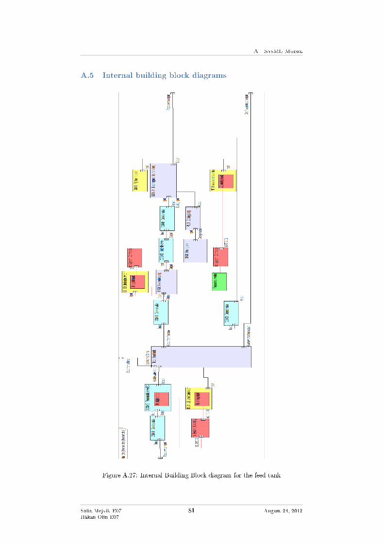
A SysML Model

A.5 Internal building block diagrams

Figure A.27: Internal Building Block diagram for the feed tank


81 August 24, 2012

A SysML Model

Figure A.28: Internal Building Block diagram for the multi-media �lter

Figure A.29: Internal Building Block diagram for the active carbon �lter


82 August 24, 2012

A SysML Model

Figure A.30: Internal Building Block for the holding tank


83 August 24, 2012

A SysML Model

A.6 Parametric diagrams

Figure A.31: Parametric diagram describing the water �ow through the mem-brane

A.7 Package diagrams

Figure A.32: Package diagram for requirements and stakeholders


84 August 24, 2012

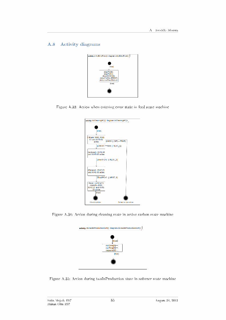
A SysML Model

A.8 Activity diagrams

Figure A.33: Action when entering error state in feed state machine

Figure A.34: Action during cleaning state in active carbon state machine

Figure A.35: Action during twoInProduction state in softener state machine


85 August 24, 2012

A SysML Model

Figure A.36: Action during ok state in Part1 state machine

Figure A.37: Action when exiting production state in Part2 state machine

Figure A.38: Action during reset state in Plant state machine


86 August 24, 2012

A SysML Model

A.9 Sequence diagrams

Figure A.39: Initial startup


87 August 24, 2012

A SysML Model

Figure A.40: State machine task cycle


88 August 24, 2012

A SysML Model

Figure A.41: Osmosis start and stop sequence


89 August 24, 2012

A SysML Model

Figure A.42: Synchronization sequence when reseting from an error


90 August 24, 2012

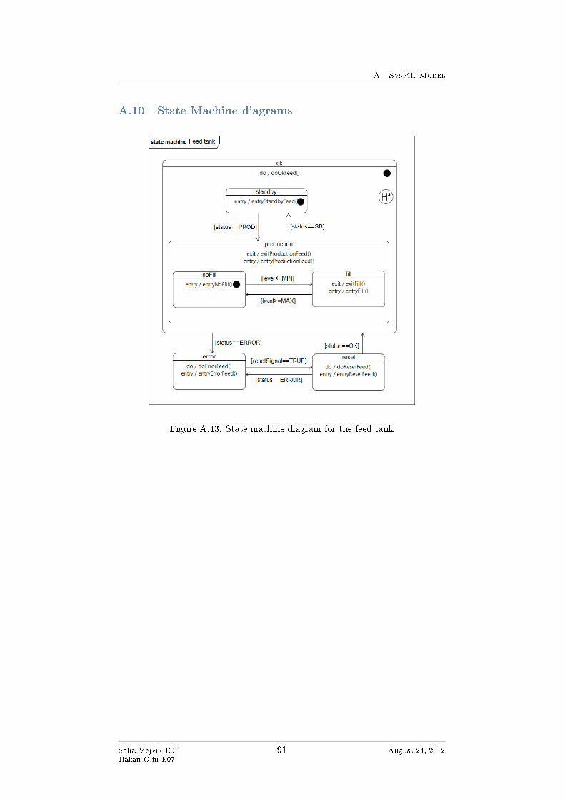
A SysML Model

A.10 State Machine diagrams

Figure A.43: State machine diagram for the feed tank


91 August 24, 2012

A SysML Model

Figure A.44: State machine diagram for the multi media �lter

Figure A.45: State machine diagram for the active carbon �lter


92 August 24, 2012

A SysML Model

Figure A.46: State machine diagram for the softener

Figure A.47: State machine diagram for Part1


93 August 24, 2012

A SysML Model

Figure A.48: State machine for Part2

Figure A.49: State machine diagram for the Plant


94 August 24, 2012

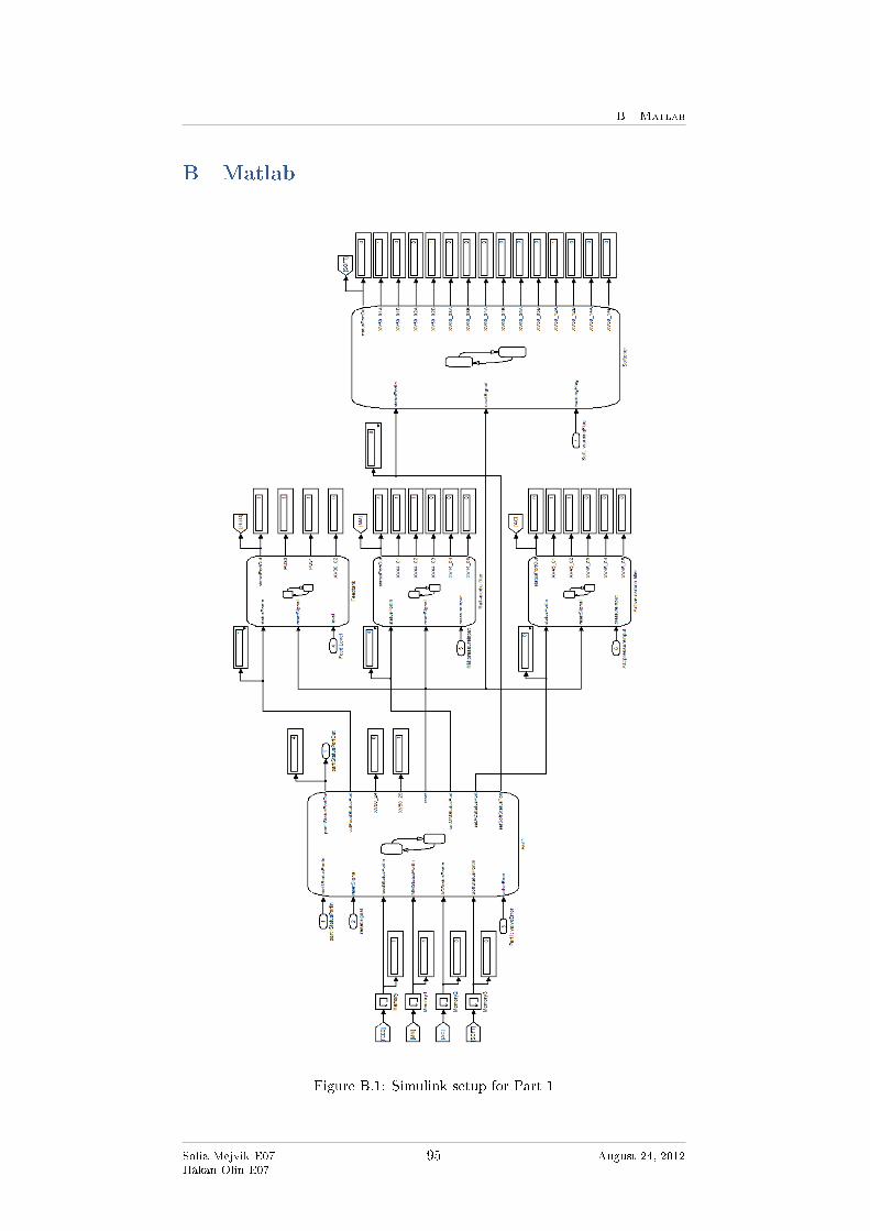
B Matlab

B Matlab

Figure B.1: Simulink setup for Part 1


95 August 24, 2012

B Matlab

Figure B.2: Simulink setup for Part 2


96 August 24, 2012

B Matlab

Figure B.3: Simulink setup for the Plant


97 August 24, 2012

B Matlab

Figure B.4: State machine diagram for feedtank

Figure B.5: State machine diagram for multimedia �lter


98 August 24, 2012

B Matlab

Figure B.6: State machine diagram for active carbon �lter

Figure B.7: State machine diagram for softener


99 August 24, 2012

B Matlab

Figure B.8: State machine diagram for Part 1

Figure B.9: State machine diagram for Part 2


100 August 24, 2012

B Matlab

Figure B.10: State machine diagram for the plant

Number Short state name Formal state name0 SB Standby1 PROD Production2 CIRC Circulation3 ERROR Error4 CLEAN Cleaning5 SAN Hot water sanitization-2 ERROR Error (Only used in Matlab)-3 OK Ok52 SAN_RO_CEDI Hot water sanitization of RO and CEDI53 SAN_RO Hot water sanitization of RO

Table B.1: Table for mapping the status number used in Matlab to the enumer-ator used in SysML.


101 August 24, 2012

C Implementation

C Implementation

Signals used:STANDBY_SPRODUCTION_SERROR_SOK_SNOFILL_SFILL_SCLEANING_SCLEANING_MM_SCLEANING_AC_SCIRCULATION_SCIRCULATION_PART1_SCIRCULATION_PART2_SRESET_SRESET_REQUEST_SREGEN_SOFTA_SREGEN_SOFTB_SHWS_SHWS_PART1_SHWS_RO_SHWS_PART2_SONE_IN_PRODUCTION_SDONE_CLEANING_SDONE_REGEN_SDONE_HWS_SDURING_S


102 August 24, 2012

Documents

Model Based Engineering of a Reverse Osmosis Water