Abstract— In this paper, we propose a new approach for model-based leak detection and location in water distribution

networks (WDN), which considers an extended time horizon analysis of pressure sensitivities. Five different ways of using

the leak sensitivity matrix to isolate the leaks are described and compared. The first method is based on the binarization

approach proposed in (Pérez, 2011a). The second, third and fourth methods are based on the comparison of the

measured pressure vectors with hte leak sensitivity matrix using different metrics (correlation, angle between vectors and

Euclidean distance, respectively); the fifth is based on the least square optimization method proposed in (Pudar, 1992).

The performance of these methods is compared when applied to two academic small networks (Hanoi and Quebra) widely

used in the literature. Finally, the three methods with better performance are applied to a district metering area (DMA)

of the Barcelona WDN using real data.

I. INTRODUCTION

Water leaks in water distribution networks (WDN) can cause significant economic losses in fluid transportation

and an increase on reparation costs that finally generate an extra cost for the final consumer. In many WDN, losses

due to leaks are estimated to account up to 30% of the total amount of extracted water. Such burden is a very

important issue in a world struggling to satisfy water demands of a growing population.

Several works have been published on leak detection and isolation methods for WDN. For example, in Colombo

et al. (2009), a review of transient-based leak detection methods is offered as a summary of current and past work. In

(Yang, 2008), a method has been proposed to identify leaks using blind spots based on previously leak detection that

uses the analysis of acoustic and vibrations signals (Fuchs, 1991), and models of buried pipelines to predict wave

velocities (Muggleton, 2002). More recently, Mashford et al. (2009) have developed a method to locate leaks using

Support Vector Machines (SVM) that analyzes data obtained by a set of pressure control sensors of a pipeline

This work was supported in part by the grants CICYT SHERECS DPI-2011-26243 and WATMAN DPI2009-13744 of Spanish Ministry of

Education and by iSense grant FP7-ICT-2009-270428 and by EFFINET grant FP7-ICT-2012-318556 of the European Commission.

Myrna Violeta Casillas and Luis Eduardo Garza are with Instituto Tecnológico y de Estudios Superiores de Monterrey, Monterrey, 64849 México (e-mail: {mv.casillas.phd.mty,@itesm.mx, legarza @itesm.mx).

Vicenç Puig is with Institut de Robòtica i Informàtica Industrial (IRI),UPC-CSIC,Llorens i Artigas,4-6,08028,Barcelona, Spain (e-

mail:vicenc.puig@upc.edu)

Model-based Leak Detection and Location in Water Distribution

Networks considering an Extended-horizon Analysis of Pressure

Sensitivities

Myrna V. Casillas Ponce, Luis E. Garza Castañón, Vicenç Puig Cayuela

network to locate and calculate the size of the leak.

Another set of methods is based on the inverse transient analysis (Covas et al, 2001, Kepler et al, 2011). The main

idea of this methodology is to analyze the pressure data collected during the occurrence of transitory events by

means of the minimization of the difference between the observed and the calculated parameters. In (Ferrante et al.

2003a; 2003b), it is shown that unsteady-state tests can be used to pipe diagnosis and leak detection. The transient-

test based methodologies are used exploiting the equations for transient flow in pressurized pipes in frequency

domain and in the second part, information about pressure waves is taken into account as well.

Model based leak detection and isolation techniques have also been studied starting with the seminal paper of

Pudar (1992) which formulates the leak detection and location problem as a least-squares estimation problem.

However, the parameter estimation of water network models is not an easy task (Savic, 2009). The difficulty lies in

the non-linear model of water networks and the few measurements usually available with respect to the large

number of parameters to be estimated that leads to an underdetermined problem. Alternatively, in (Pérez, 2011a;

2011b), a model based method that relies on pressure measurements and leak sensitivity analysis is proposed. This

methodology consists in analyzing the residuals (difference between the measurements and their estimation using

the hydraulic network model) on-line regarding a given threshold that takes into account modeling uncertainty and

the noise. When some of the residuals violate their threshold, the residuals are compared against the leak sensitivity

matrix in order to discover which of the possible leaks is present. Although this approach has good efficiency under

ideal conditions, its performance decreases due to the nodal demand uncertainty and noise in the measurements.

This methodology has been improved in (Casillas et al. 2012) where an analysis along a time horizon has been taken

into account and a comparison of several leak isolation methods is offered. In case where the flow measurements are

available, leaks could be detected more easily since it is possible to establish simple mass balance in the pipes. See

for example the work of Ragot (2006) where a methodology to isolate leaks is proposed using fuzzy analysis of the

residuals. This method finds the residuals between the measurements with and without leaks. However, although the

use of flow measurements is viable in large water transport networks this is not the case in water distribution

networks where there is a dense mesh of pipes with only flow measurements at the entrance of each District

Metering Area (DMA). In this situation, water companies consider as a feasible solution the possibility to installing

some pressure sensors inside the DMAs. Pressure sensors in this situation are preferred because they are cheaper and

easy to install and maintain.

Recently, Goulet et al. (2013) proposed a model falsification leak detection and isolation approach as well a

sensor placement for leak detection and isolation technique. Here, a leak–scenario falsification is developed in order

to evaluate the performance of the network as well as to model and to measure the uncertainties during the leak

detection process. However, this work is able to find leaks of big magnitudes and needs a large instrumentation in

pipes.

The model calibration of a water distribution network is an important problem related to the leak detection task

because the leakages are not all real. In (Koppel et al. 2012), an optimization procedure is proposed to obtain the

proportion of real and apparent leakages. There are some works devoted to the prediction and correction of models.

An hydraulic state estimation technique using statistical data to estimate future demands is proposed in (Preis et al.

2011). This work uses genetic algorithms to calibrate the model with a modified least squares fit method. Model

calibration using genetic algorithms is also studied in (Nicolini et al. 2011, Shu 2010). Nodal demand calibration has

been studied (Cheng et al. 2011) using singular value decomposition in order to identify and understand the

parameters of the model. However, for a limited number of monitoring sensors, this problem is underdetermined and

the parameter estimation is too complex. Herrera et al. (2010) offer a description and comparison of predictive

models for forecasting water demand where models are obtained using time series data for water consumption in an

urban area of a city and applying predictive regression models, machine learning algorithms and Monte Carlo

simulations. In Wu et al. (2010), a method for leakage detection and hydraulic model calibration is presented. This

work shows that leak detection improves with the accuracy of the hydraulic model calibration and by identifying the

unknown leakages and the non-revenue water consumptions. Moreover, this research demonstrates that water

utilities can exploit the latest innovations of modeling technology to manage, detect, control and reduce water

leakages. Wu et al. (2011), find that velocities and head loss needs to be increased over normal values for the

pressure based leak detection work. They found that the effect of closed valves and model errors obscures leaks.

In this paper, a new approach for model-based leak detection and location in water distribution networks (WDN)

is presented. This approach considers an extended time horizon analysis of pressure measurements and sensor leak

sensitivities. This approach has been combined with five leak location methods in order to find the best one. A first

method, called Sensitivity Matrix Binarization, is based on the transformation of the real-valued leak sensitivity

matrix to a binary matrix, according to a threshold as suggested in (Pérez 2011a; 2011b). Three methods are based

on the comparison of measured pressure vectors with leak sensitivity matrix using different metrics (Correlation,

Angle between vectors and Euclidean distance, respectively). Finally, also a method based on the Least-square

optimization method proposed in (Pudar, 1992) is tested. In order to find the method with the best performance, the

five methodologies are tested in simulation with two academic small water distribution networks (named Hanoi and

Quebra) assuming that the pressures in all the nodes are measured. Finally, the three methods with better

performance are applied to a district metering area (DMA) of the Barcelona WDN, named Nova Icària, considering

that only few sensors are available in practice which implies more difficulties in determining the leakage area.

This paper is organized as follows: Section II describes an overview of the proposed methodology. Section III

explains the leak location strategies. Section IV presents the networks considered in the experiments including the

Barcelona WDN. In Section V, the experiments and results for the academic networks are detailed while in Section

VI, the application and results obtained with the different methodologies in the real case are presented. Finally,

Section VII concludes this work.

II. OVERVIEW OF THE PROPOSED METHODOLOGY

A. Introduction

The main objective of the proposed methodology is to detect and isolate leaks in a water distribution network

using pressure measurements and their estimation using the hydraulic network model. A leak will be considered as a

water flow loss through a defect of a network element that is being monitored. The proposed approach assumes the

existence of a single and continuous leak from the appearance time. Moreover, all the leaks are assumed to be

located in the nodes of the network. This is a standard assumption in model based leak detection and location

literature (see for example, Pudar (1992)).

The leak detection is based on computing the difference (residual) between the pressure measurements ( )ip k

against their estimation ˆ ( )ip k by means of the simulation of the hydraulic model:

𝑟𝑖(𝑘) = 𝑝𝑖(𝑘) − �̂�𝑖(𝑘) 𝑖 = 1, … , 𝑛 (1)

where 𝑛 is the number of pressure sensors available in the network. These residuals are evaluated against a threshold

i that is selected to take into account the measurement noise and model uncertainty. If for a given time window a

residual violates its threshold (i.e, ( )i ir k ) then, the location process is initiated. The leak location is based on

comparing the residual vector (obtained from the difference between measured and expected pressures of each

sensor) against the leak sensitivity matrix that contains the effect of each possible leak in each residual. The

candidate leaks are those whose effect matches the best in a time window when compared to the observer residual

vector using some metric (see Section III for more details). Once the candidate leak has been isolated, an estimation

of the leak could even be provided by means of the residual leak sensitivity. Figure 1 summarizes graphically the

proposed methodology including the leak detection, location and estimation processes.

Figure 1 Proposed methodology for model based leak detection, location and estimation.

Remark 1: As any model based approach, the results of the proposed methodology rely on the quality of the model.

Thus, leaks will not be detected if the effects of leaks on pressure are masked by the cumulative effect of model

errors (e.g. connectivity, closed valves) and demand variations not accounted for by the model.

Remark 2: Unexpected demands changes due to special days/events or some test/changes in the network could

induce the methodology to indicate a leak when in fact there is not (false positives). For this reason, the proposed

methodology should be used in combination with the DMA monitoring methodology proposed in (Quevedo et al.,

2012) that analyses the night flows altogether with the supplied/billed amount of water. When a leak is detected with

the methodology, then proposed leak location could be safely used to locate approximately where the leak is located.

Finally, the technicians will go to field using acoustic based leak location equipment to precisely locate the point

where the leak is and to repair it.

B. Leak sensitivity matrix

As discussed above, leak location is based on the evaluation of the effect of all possible leaks in the available

pressure measurement sensors using a sensitivity analysis. As a result of this analysis the sensitivity matrix (Pérez,

20009a) is obtained as follows:

𝑺 =

[ 𝜕𝑝1

𝜕𝑓1⋯

𝜕𝑝1

𝜕𝑓𝑚⋮ ⋱ ⋮

𝜕𝑝𝑛

𝜕𝑓1⋯

𝜕𝑝𝑛

𝜕𝑓𝑚]

(2)

where each element ijs of the sensitivity matrix S measures the effect of a leak jf in the pressure of sensor ip (i.e.

the difference of pressure between the expected pressure and the one measured when a leak of magnitude f occurs in

the node j). Each element is normalized according to the leak magnitude. The sensitivity matrix S has as many rows

as sensors and as many columns as considered leaks. It is extremely complex to calculate S analytically in a real

network since the model is based on a huge set of implicit non-linear equations. Instead, this work proposes to

generate the sensitivity matrix by simulation thanks to an hydraulic simulator (as EPANET) and using increments of

pressure while maintaining constant the leakage flow. First, the computation of the sensitivity matrix needs the

construction of the non-faulty operation scenario of the network in a 24-hours’ time horizon, which allows to obtain

the vector 𝒑(𝑘) for the non-faulty pressure of each node of the network

𝒑(𝑘) = [𝑝1(𝑘)

⋮𝑝𝑛(𝑘)

] (3)

where 𝑝𝑖(𝑘) represents the pressure of node 𝑖 at time 𝑘 without the presence of leak and n is the number of sensors

in the network.

Then, leak scenarios are considered in simulation by introducing a leak at a time in each node of the network. The

pressures of the sensors in case of each considered leak scenario are stored in the matrix:

𝑷𝒇 (𝑘) = [𝑝1

𝑓1(𝑘) ⋯ 𝑝1𝑓𝑚(𝑘)

⋮ ⋱ ⋮

𝑝𝑛𝑓1(𝑘) ⋯ 𝑝𝑛

𝑓𝑚(𝑘)

] (4)

where 𝑝𝑖

𝑓𝑗(𝑘) is the pressure of the sensor 𝑖 at time instant 𝑘 when a leak is present at node 𝑗, m is the number of

nodes in the network (possible leaks) and n is the number of sensors in the network.

Finally, using vector (3) and matrix (4), the sensitivity matrix S for each time instant of the horizon considered is

computed as follows

𝑺(𝑘) =

[ 𝑝1

𝑓1(𝑘) − 𝑝1(𝑘)

𝑓1⋯

𝑝1𝑓𝑚(𝑘) − 𝑝1(𝑘)

𝑓𝑚⋮ ⋱ ⋮

𝑝𝑛𝑓1(𝑘) − 𝑝𝑛(𝑘)

𝑓1⋯

𝑝𝑛𝑓𝑚(𝑘) − 𝑝𝑛(𝑘)

𝑓𝑚 ]

(5)

where each element 𝑠𝑖𝑗(𝑘) measures the effect of leak 𝑓𝑗 in the pressure of sensor 𝑝𝑖 at the instant 𝑘. Thus, the

sensitivity matrix is composed of (n × m) elements where each element is determined by computing the difference

between the non-leaky and the leaky pressure obtained by simulation normalized with respect to the magnitude of

the leak used to obtain the sensitivity matrix.

III. LEAK LOCATION SCHEMES

Leak location is based on analyzing the residuals (1) along the proposed time horizon, trying to find some

inconsistency between the pressure measurement and their estimated value in order to establish which node is the

most affected and thus has the highest probability of presenting leakage. In this paper, a comparison of five

different methods to isolate leaks that use the sensitivity matrix (5) is performed. The proposed methods can be

divided in direct and indirect methods. The direct methods can be classified as binary or non-binary. The non-binary

direct methods considered are based on residual correlation, Euclidean distance and the angle of the residual vector

with the leak signature vectors stored in the sensitivity matrix. On the other hand, the indirect method is based on a

least-square optimization method. In all these methods, a sensitivity matrix (2) that quantifies the effect of all

possible leaks in all nodes and pressure sensors in the network is needed to initiate the detection of the leak. The

five approaches are described in the following.

A. Binarized sensitivity method

The binarized sensitivity method works as follows (see Pérez et al. (2011a) for more details):

a) The sensitivity matrices (5) are binarized according to an established threshold

b) 𝑠𝑖𝑗𝑏𝑖𝑛(𝑘) = {

1 𝑖𝑓 𝑠𝑖𝑗(𝑘) > 𝜌

0 𝑜𝑡ℎ𝑒𝑟𝑤𝑖𝑠𝑒 (6)

where 𝑠𝑖𝑗𝑏𝑖𝑛(𝑘) represents the element of the 𝑺𝒃𝒊𝒏(𝑘) sensitivity.

b) The current residual vector 𝒓(𝑘) defined in (1) is computed and binarized in a similar way than the

sensitivity matrix in the previous step

𝑟𝑖𝑏𝑖𝑛(𝑘) = {1 𝑖𝑓 𝑟𝑖(𝑘) > 𝛽

0 𝑜𝑡ℎ𝑒𝑟𝑤𝑖𝑠𝑒 (7)

where 𝑟𝑖𝑏𝑖𝑛(𝑘) are the elements of the actual residual vector 𝒓𝒃𝒊𝒏(𝑘).

c) The residual vector is compared against each column of the sensitivity matrix. When the algorithm finds a

matching at given time instant, i.e. 𝒓𝒃𝒊𝒏(𝑘) = 𝒔−,𝒋𝒃𝒊𝒏(𝑘), then the leak 𝑓𝑗 associated to the column j that

matches is indicated as a candidate leak.

d) Because the leaks are analyzed for a time horizon of 24 hours, it is necessary to count the coincidences

found on previous step in order to find the leak with the maximum number of coincidences. As result of

this comparison, a matrix 𝚽 is created in which the binary indicators of the existence or absence of the

leak will be saved

𝜙𝑗𝑘 = {1 if 𝒓𝒃𝒊𝒏(𝑘) = 𝒔−,𝒋

𝒃𝒊𝒏(𝑘)

0 otherwise 𝑗 = 1, … ,𝑚 (8)

and where k is the time instant. To calculate the leak in the time horizon, we look for the index that appears

the most through the time horizon L and this index is assigned as the leak index during the considered time.

This is formulated as follows:

𝛾𝑗 = ∑ 𝜙𝑗(𝑘)

𝐿

𝑘=1

(9)

where 𝜸 is a vector that contains the number of fault indications for the possible leaks according to the row

that is occupying. Thus, if the maximum of this vector is found, then the index of the node that contains the

leak in the desired time horizon is obtained by

𝑙𝑒𝑎𝑘𝑖𝑛𝑑𝑒𝑥 = 𝑎𝑟𝑔 𝑚𝑎𝑥𝑗∈{1,⋯,𝑚}

(𝛾𝑗). (10)

e) Finally, the leak magnitude can be estimated using the residual vector (1) and the sensitivity matrix column

corresponding to the candidate leak 𝑓𝑗 identified using (10).

min𝑓𝑗∑ |𝒓(𝑘) − 𝒔−,𝑗(𝑘)𝑓𝑗|

2 𝐿

𝑘=1 (11)

B. Angle between vectors method

The angle method is based on evaluating the angle between the current residual vector 𝒓(𝑘) and each column of

the leak sensitivity matrix as follows

𝛼𝑗(𝑘) = 𝑎𝑟𝑐𝑐𝑜𝑠 (𝒓𝑻(𝑘)𝒔−,𝒋(𝑘)

|𝒓(𝑘)||𝒔−,𝒋(𝑘)|) 𝑗 = 1… ,𝑚 (12)

Then, the mean angle in the selected time horizon L is computed as:

𝛼�̅� =1

𝐿∑ 𝛼𝑗(𝑘)

𝐿

𝑘=1

𝑗 = 1, … ,𝑚 (13)

and the candidate leak proposed is the one that presents the smallest mean angle

j

indexj 1,…,m

leak = arg min (14)

After locating the leak, its magnitude can be estimated using the residual vector and the leak sensitivity matrix using

(11).

C. Correlation method

The correlation method is based on correlating the current residual vector 𝒓(𝑘) with each column of the leak

sensitivity matrix as follows

𝑐𝑗𝑘 =

∑ (𝑟𝑖(𝑘) − 𝑟(𝑘)̅̅ ̅̅ ̅̅ )(𝑠𝑖𝑗(𝑘) − 𝑠𝑗(𝑘)̅̅ ̅̅ ̅̅ ̅)𝑛𝑖=1

√∑ (𝑟𝑖(𝑘) − 𝑟(𝑘)̅̅ ̅̅ ̅̅ )2𝑛

𝑖=1√∑ (𝑠𝑖𝑗(𝑘) − 𝑠𝑗(𝑘)̅̅ ̅̅ ̅̅ ̅)

2𝑛𝑖=1

𝑗 = 1, … ,𝑚 (15)

where ( )r k is the mean of the k residual vector and 𝑠𝑗(𝑘)̅̅ ̅̅ ̅̅ ̅ represents the average along the j vector of the k

sensitivity matrix.

Then, the mean correlation in the selected time horizon L is computed and the candidate leak proposed is the one

with the smallest value.

𝑐�̅� =1

𝐿∑ 𝑐𝑗(𝑘)

𝐿

𝑘=1

𝑗 = 1, … ,𝑚. (16)

Then, looking at the maximum correlation along the time horizon, we can find the leaky node as follows

index j

j 1,…,mleak = arg min (c ) .

(17)

As in the previous method, after locating the leak, its magnitude can be estimated using the residual vector and

the leak sensitivity matrix using (11).

D. Euclidean distance method

Alternatively to the previous methods, the Euclidean distance between the current residual vector 𝒓(𝑘) and each

column of the leak sensitivity matrix can be used to isolate the leaks at a given instant time

𝑑𝑗(𝑘) = √∑(𝑟𝑖(𝑘) − 𝑠𝑖𝑗(𝑘)𝑓𝑛𝑜𝑚)2

𝑛

𝑖=1

𝑗 = 1,⋯ ,𝑚 (18)

where fnom is the nominal leak used to compute sij and is different from fj computed using (11). Then, the distance

vector for the time horizon is calculated as

�̅�𝑗 =1

𝐿∑ 𝑑𝑗(𝑘)

𝐿

𝑘=1

𝑗 = 1, … ,𝑚 (19)

Since each element of this vector represents the Euclidean distance to every possible leak, we conclude that the

candidate leak can be found determining the minimum value of that vector

jindexj 1,…,m

leak = arg min d (20)

This method only when the leak has the same magnitude as the one used to compute the sensitivity matrix. If it is

not the case, it does not provide good results.

Similarly to what is performed when using the previous methods, after the leak is located, its magnitude can be

estimated using the residual vector and the leak sensitivity matrix using (11).

E. Least square optimization method

This method works in an opposite way than the other methods, i.e. it computes an inverse optimization problem in

order to find an appropriate leak size that explains the pressure measurements present in every node. Then, it

performs an analysis of the minimum error in order to find the node affected by a leak.

This method also uses the leak sensitivity matrix and solves the following optimization problem for each

candidate leak:

1, ,j mjj

L2

f -, j jf

k=1

J = min k - k fr s( ) ( ) (21)

Then, the leaky node is found as the one that produces the smallest index

jfJindex

j=1,…,mleak = arg min (22)

As one can see, this method allows obtaining more information about the leak since it provides the leak size that

fits the best for the observed pressure data. The leak that provides the smallest value in (22) is the candidate leak.

IV. DESCRIPTION OF THE WATER NETWORKS USED IN THE EXPERIMENTS

To test the aforementioned methodologies, two academic networks were used. The Hanoi network (from

Fujiwara, 1990), and the Quebra network (provided as an example coming with EPANET software). As discussed in

Section II, all the leaks are located in the nodes of the network. In simulation, this can be performed in two ways.

The first one is to add an extra demand of water at a specific node and to use two patterns of water demands: one to

simulate the non-leaky water demand and the other one to simulate the leak. A secondary is to find the

corresponding emitter coefficient that provides the desired leak magnitude in the network. In (Rossman, 2000), it is

shown that in EPANET the emitter coefficient is specified for individual leaks according to the equation:

𝐸𝐶 = 𝑄/𝐹𝑝 𝑃𝑒𝑥𝑝 (23)

where 𝐸𝐶 (in 0.5

lps

m ) is the emitter coefficient, 𝑄 is the flow rate, 𝐹𝑝 is the fluid pressure and 𝑃𝑒𝑥𝑝 is the pressure

exponent.

In the academic networks used in this paper, the leak is simulated as an extra demand with a unitary pattern along

the time horizon considered, i.e. we will take into account that the leak is single and continuous along a determinate

time window. In the contrary in the real case application of the Barcelona Network, the leak is simulated using an

emitter coefficient approach described previously. This allows us to consider that leaks depend as well of the

pressure in the node where they appear.

To compare the efficiency of each location method presented in Section III, changes in the leak magnitude, noise

in the measurements and nodal demands were simulated. A time horizon window of 24 hours was considered for the

simulations. Matlab®

and Epanet were combined to simulate the leaks and to obtain and analyze the network data

using the algorithms proposed in the paper.

A. Hanoi network

This network is presented in Figure 2. It will allow us to analyze the effectiveness of the proposed methods in a

network with big flows.

The demand pattern is designed according to (Fujiwara et al 1990). A simulation of 24 hours with a sampling time

of 15 minutes is carried out. This is because the demand is measured each 15 minutes. This gives a total of 97

samples.

Figure 2 Diagram of Hanoi network

This network has 31 demand nodes with indexes from 2 to 32. A leak with a magnitude of 50 liters per second is

used to compute the sensitivity matrices shown in Figure 3.

Figure 3 Leak sensitivity matrices for the Hanoi network

B. Quebra network

This network is presented in Figure 4. It will allow analyzing the performance of the proposed methods using a

network of bigger size than the Hanoi network. Quebra is a network designed according to the method presented in

the EPANET webpage.

Figure 4 Diagram of Quebra network

In this network, the demand is measured with a sampling time of one hour. The simulation is carried out for 24

hours giving a total of 25 samples (0-24h). The following parameters used in the simulation of the network are

established: The network is composed of 55 nodes and the samples are taken every hour. The sensitivity matrices are

calculated with a leak magnitude of 0.01 liters per second. Figure 5 shows the values of the sensitivity matrix for

node 34 at the sample instant of maximum consume (left) and with a leak (right).

Figure 5 Leak sensitivity matrices for Quebra network

In Hanoi and Quebra academic networks, the leak magnitude used to compute the sensitivity matrix and those

magnitudes for the simulated leaks are chosen according to the observed demands along the time horizon. The idea

is to introduce leaks that, based on the considered, will affect the pressur in order to probe that the methodology can

be applied. Later we will see what happens when we apply the methods in a real case.

C. Barcelona network

Finally, the proposed approach is applied to a real network simulated in EPANET. This network is located in

Nova Icaria area in Barcelona, Spain. It is composed of 3320 nodes, where 1900 are demand nodes and the rest is

used to simulate street or junction nodes. In our case, we propose to simulate the possible leaks for the total of 3320

nodes. Using the method presented in (Pérez, 2009b), a first optimal sensor placement of 15 sensors where

considered (see Figure 6). Later, taking budget restrictions of the Barcelona water company, 6 sensors were installed

optimally located using the same method proposed in (Pérez, 2009b) (see Figure 7).

Once we know the localization of the sensors, we can establish the parameters to compute the sensitivity matrices.

When 15 sensors are used, sensitivity matrices are evaluated with a nominal leak of 3 lps which corresponds to an

emitter coefficient of EC=0.48 and in the case of 6 sensors, we propose an EC=0.25. The reason for using these

values comes from the fact that in a first trial we took 15 sensors within our experimentation, trying to isolate leaks

whose magnitudes were between 0.7 and 6.3 liters per second. Then, when the first part of the work was done, we

decided to change the size of the nominal leak, knowing that the leak sizes to be located, according to the water

company, are between 0.7 and 3 liters per second. In the same way, we noticed from the results obtained in the first

part of the experimentation that when the real leak is close to the value of the nominal leak, it can be located more

easily.

Figure 6 Optimal sensor placement in the case of 15 sensors for the Nova Icaria network.

Figure 7 Optimal sensor placement in the case of 6 sensors as validated by the water company for the Nova Icaria network.

V. APPLICATION TO THE ACADEMIC NETWORKS

A. Experiments

In the case of the academic networks, the following experiments were developed to test the proposed methodologies:

1. Impact analysis of the leak magnitude.

2. Application of random demand noise between ±2% and ±4% of the medium demand along the time horizon.

3. A study of the effect of the measurement noise, applying Gaussian white noise around of ±2% of the pressure

measurements.

4. Application of both uncertainties introduced in Step 2 and Step 3

5. Finally, both effects were tested with 200 random leaks location with and without noise whose size depends on

the network, i.e., with sizes around 20 to 80 liters per second for the Hanoi Network, and from 0.01 to 1 liter per

second for the Quebra network.

In all the experiments performed, the proposed angle method is compared first with the least square optimization

method and then with the correlation method. In all the cases, the efficiency achieved by each method is evaluated

and compared with the one achieved when all the network pressures are fully accessible.

B. Results

The results of tests 1, 2, 3 and 4 are shown in Table I and Table III. It can be observed that each method delivers

very good results. The results of test 5 are shown in Table II and Table IV where it can be observed that best method

is the proposed angle between vectors.

In all the tables, the effectiveness is shown in percentage obtained according to the number of leaks detected

satisfactorily divided by the number of tests realized. It is important to mention that the network structure has an

important impact in the results. It means that introducing appropriate structural changes in the network, even better

performance of the methods could be achieved.

Table I

Efficiency (%) in tests applied to the Hanoi network

TEST OF EFFECT OF 2% NOISE ON DEMAND AND MEASUREMENTS

Leak size Binarization Correlation Angle Distance Optimization

50 51.61 96.77 100 100.00 96.77

10 38.71 83.87 90.32 3.23 83.87

20 38.71 93.55 96.77 3.23 87.1

30 38.71 90.32 96.77 6.45 90.32

40 51.61 96.77 100 32.26 100

60 58.06 96.77 100 54.84 93.55

70 58.06 96.77 100 45.16 96.77

80 61.29 96.77 100 38.71 100

Average efficiency 48.76 93.84 97.93 35.48 93.38

Table II

Efficiency (%) in random tests for the Hanoi network

Test Binarization

method

Correlation

method

Angle

method

Distance

Method

Optimization

method

No noise 100 100 100 33.33 100

Demand noise 86 90 98 46.67 94

Measure noise 60 70 98 60 98

Noise in both 48 60 98 46.67 96

Table III

Efficiency (%) in tests applied to Quebra network

TEST OF EFFECT OF 2% NOISE ON DEMAND AND MEASUREMENTS

Leak size Binarization Correlation Angle Distance Optimization

0.01 62.96 88.89 92.59 98.15 88.89

0.03 46.3 79.63 81.48 1.85 85.19

0.02 66.67 94.44 94.44 46.30 94.44

0.08 79.63 98.15 98.15 20.37 98.15

0.15 83.33 96.3 98.15 16.67 98.15

0.2 85.19 96.3 98.15 16.67 98.15

Average efficiency 69.2 92.05 93.63 19.04 93.69

Table IV

Efficiency (%) in random tests for Quebra network

Test Binarization

method

Correlation

method

Angle

method

Distance

method

Optimization

method

No noise 98 100 100 26.67 100

Demand noise 98 100 100 33.33 100

Measure noise 72 94.5 97.5 40.00 98

Noise in both 71.5 94.5 98.5 13.33 98.25

Seeing tables presented above, we are able to conclude that binarization and Euclidean distance methods are not

efficient enough locating leaks. In the case of binarization method, this may be due to the fact that we have to

establish a threshold in order to binarize the vectors and in several cases it is not possible to know the correct value.

In the case of the Euclidean distance, noise factors and demand pattern changes tend to decrease the similarity

between corresponding vectors and becomes difficult the location. However, we have seen that correlation,

optimization and the proposed angle method can be efficient techniques in the leak location task. After analyzing the

result of the tests, it can be concluded that methods based on optimization and vector angle provide excellent results.

VI. APPLICATION TO THE BARCELONA WATER NETWORK

A. Experimental scenarios

From the tests performed in the academic networks, we noticed that the angle, optimization and correlation

methods have a better efficiency regarding the localization task when all the pressure measurements are available.

In order to test the performance of the considered methods in the real case where not all pressure measurements are

available, several scenarios have been proposed in this paper. In these scenarios, we test:

- the location of a nominal leak without noise,

- the location of non-nominal leak without noise,

- the location of non-nominal leak with noise.

In the previous scenarios nominal means that the leak has the same magnitude as the one used to compute the

sensitivity matrices, while non-nominal means that the leak has a different magnitude.

This section shows the results obtained when considering only one of the leaky nodes, subject to different conditions

corresponding to the scenarios described below and for the methods considered in the network. In the figures

showing leak location results, the nomenclature presented in Figure 8 will be used.

Figure 8 Nomenclature for the leak location results.

1) 15 sensors case

The first scenario involves the presence of a nominal leak affecting the network. In this case, the three methods

find exactly the node where the leak is present. Figure 9 presents the location of a nominal leak without noise

applying the angle method. In that case, the correct location of the leak node is achieved, as noticed, the absence of

noise and nominal leak magnitude tested, facilitate the location of the leak.

Figure 9 Location of a nominal leak without noise applying the angle method.

The second scenario involves the presence of a nominal leak taking also into account noise in the measurements

and in the demands. In this case, the method efficiency is reduced. In Figure 10, we can see how the angle method

locates the leak near to the real leak, while in Figure 11 we see that using the optimization method, the distance is

slightly higher than using the angle method.

Figure 10 Location of a nominal leak in presence of noise and when applying the angle method. The leak node is found only 6.14 meters

farther than the real leakage node.

Figure 11 Location of a nominal leak in presence of random noise, when applying optimization method The leakage node was located 14.24

meters farther than the real leak.

The third scenario corresponds to the case where there is a non-nominal leak present in the network and where

the noise can be taken into account or not. In the experiments, we took the example of leaks whose magnitude

varies from 0.7 and 6.3 liters per second. Figure 12 shows the behavior of the angle method when a non-nominal

leak is occurring, despite the presence of noise, a leak is found near of the correct leak. Figure 13 shows the same

experiment using the optimization method, where the distance found is higher than with the angle method.

Finally, in Figure 14, we show the case of non-nominal leak and when random noise is added using the

correlation method. In that case, the behavior is very similar to the one obtained with the optimization method.

Figure 12 No nominal leak location using the angle method. Despite the presence of noise, the leakage node is found at a distance of only 5.92

meters from the real leak location.

Figure 13 Leak location of a 0.7 lps magnitude leak in case of random noise using the optimization method. The leakage node was located

142.52 meters from the real leak.

Figure 14 No nominal leak location using the correlation. The leakage node is found at 151.44 meters from the real leak node.

2) 6 sensors case

Similarly to the experiments where 15 sensors are involved, we performed the analysis for the case where 6

sensors are installed. Below, we detail the behavior of the methods for the same type of scenarios as the ones

previously presented. When a nominal leak without noise affects the network, the three methods find the exact leak

location. The behavior of the methods in the case of a non-nominal leak and taking into account the presence of

random noise is shown in the following. In Figure 15, we observe that using the angle method, even when only six

sensors are present within the network, the potential leak is located about only 82 meters from the real leak. Figure

16 shows the behavior of the optimization method taking into account the same case. As we can see, the leak is

located further than using the angle method. Finally, using the correlation method to locate the same leak, the

distance obtained is farther than the one obtained with the angle method but nearer than using the optimization

method as we can see in Figure 17.

Figure 15 Location of a non- nominal leak of a 6.3 lps magnitude in case of random noise. Using the angle method, the leakage node was

located 82.76 meters from the real location.

Figure 16 Location of a non-nominal leak using the optimization method. The presence of noise causes that the leakage node is found at a

distance of 270.06 meters from the real leak node.

Figure 17 Location of a non-nominal leak of a 6.3 lps magnitude in case of random noise using the correlation method, the leakage node was

located 149.72 meters from the real leak.

Another important case is when a leak begins during the process of simulation in a given point of the time horizon.

Such a situation is shown in Figure 18 where the pressure and the demand change when a leak appears at the hour 8.

Pressure is measured in meters water column and demand in liters per second.

As one can see, the difficulty in this case is that when the leak appears at a given instant of the time horizon, it

may be difficult to discriminate between measurement noise and a significant variation, i.e. the very small pressure

change can lead to some confusion in the location process.

Figure 18 Behavior of the demand and the pressure in case of a single leak appearing at the 8th hour in the time horizon. It shows that the

pressure varies only slightly and that the noise may affects the detection and location.

B. Results

In the previous section, we have seen examples of results obtained for different types of scenarios. Here, we give a

brief summary of the results obtained for each experiment performed and also a result discussion is provided.

In the following, we find the tables that sum up the efficiencies for each experiment.

1) Angle method

We first present the results in the case of 15 sensors and then the results in the case of 6 sensors. With 15 sensors,

by computing a test where every possible leak was considered (i.e. we have simulated one by one all the possible

leaks in the network), we observe how many have been found at the correct location which gives us the

corresponding efficiency percentage of location. After performing this test, we found that the angle method is able to

find the exact leakage node for 83.04% of the nodes, while almost 90% are localizable within a distance lower than

to 2 meters from the real leak. According to the results of this test, we can say that 230 of the 3220 nodes are non-

localizable in the network or have a low level of confidence. In Table V, we can see the efficiency for a test where

100 leak simulations have been performed using the angle method and 15 sensors. We observe that the mean

distance even in cases with noise is lower than 200 meters.

Table V

EFFICIENCY IN THE RANDOM LEAKS LOCATION WITH THE ANGLE METHOD AND USING 15 SENSORS

Leak Size (lps) Maximum Distance

(m) Mean Distance (m) Distance Between Ranges* (%) Random Noise

3 (Nominal) 7.85 0.24 96 No

0.7 504.86 75.46 61 No

1.7 602.52 72.79 59 No

6.3 728.11 75.95 60 No

3 (Nominal) 331.44 109.66 60 Yes

0.7 706.32 191.82 36 Yes

1.7 723 135.88 51 Yes

6.3 564.4 86.91 71 Yes

*Ranges are: 3m for nominal leak without noise, 50m for non-nominal leak without noise, 100m for leak with noise.

With 6 sensors and performing the mentioned location ability test, the ability to find the exact node is now

80.06%, 88% of possible leaks are located within a distance lower than 2 meters and there are 266 non-localizable

nodes. In Table VI, we can see the efficiency of the angle method when only 6 sensors are installed.

Table VI

EFFICIENCY IN THE RANDOM LEAKS LOCATION WITH THE ANGLE METHOD AND USING 6 SENSORS

Leak size (lps) Maximum distance

Mean distance (m) Distance between ranges* (%) Random Noise

(m)

1.67 (Nominal) 383.37 17.50 82 No

0.7 471.19 74.44 58 No

3 284.22 53.03 64 No

6.3 444.71 129.11 34 No

1.67 (Nominal) 479.41 101.95 66 Yes

0.7 449.15 119.88 58 Yes

3 525.97 103.88 68 Yes

6.3 554.85 112.27 58 Yes

*Ranges are: 3m for nominal leak without noise, 50m for non-nominal leak without noise, 100m for leak with noise.

These experiments show that the angle method is able to detect and isolate single leaks in a real network even in

the worst case with a maximum distance of approximately 700 meters. However, it is remarkable to note that the

mean distance for each experiment is close to 100 meters in presence of random noise. It is important to note that

even when the number of sensors is reduced, the efficiency of the method is not severally affected. It means that we

may reduce significantly the instrumentation of the network without affecting too much the efficiency of the

location.

2) Optimization method

Similarly to the angle method, the “leak location test” was performed for the optimization method. In the case of 15

sensors, by computing the mentioned test, we found that the method is able to find the exact leakage node for

81.08% of the nodes, while 89% are localizable within a distance lower than to 2 meters from the real leak.

According to the results of this test, we can say that 212 of the 3220 nodes are non-localizable in the network or

have a low level of confidence. With 6 sensors and according to the leak location test, the capacity of finding the

exact node is in the case of optimization method 74.25%, while the percentage of finding a node within a distance

lower than 2 meters is 84.78%. In

Table VII and Table VIII we can see the efficiency of the optimization method in the case of 15 and 6 sensors

installed respectively.

Table VII

EFFICIENCY IN THE RANDOM LEAKS LOCATION WITH THE OPTIMIZATION METHOD AND USING 15 SENSORS

Leak size (lps) Maximum distance (m) Mean distance (m) Distance between ranges* (%) Random Noise

3 (Nominal) 1.04 0.04 100 No

0.7 476.19 84.34 52 No

1.7 1250.9 55.12 72 No

6.3 551.56 66.07 61 No

3 (Nominal) 331.44 109.66 56 Yes

0.7 1218.6 188.41 37 Yes

1.7 1046.4 146.07 56 Yes

6.3 760.63 99.18 68 Yes

*Ranges are: 3m for nominal leak without noise, 50m for non-nominal leak without noise, 100m for leak with noise.

Table VIII

EFFICIENCY IN THE RANDOM LEAKS LOCATION WITH THE OPTIMIZATION METHOD AND USING 6 SENSORS

Leak size (lps) Maximum distance (m) Mean distance (m) Distance between ranges*

(%) Random Noise

1.67 (Nominal) 15.04 1.34 88 No

0.7 754.06 89.48 56 No

3 1251.8 123.85 40 No

6.3 768.85 181.1 26 No

1.67 (Nominal) 794.52 143.95 56 Yes

0.7 595.56 150.27 48 Yes

3 684.16 155.86 56 Yes

6.3 769.16 209.92 44 Yes

*Ranges are: 3m for nominal leak without noise, 50m for non-nominal leak without noise, 100m for leak with noise.

We have to highlight that even when the optimization method behavior is not as good as the angle method, it has

the advantage that it provides an approximate leak magnitude and an error in the optimization that can be exploited

as an extra information in order to improve the leak detection and location process.

As we can see from the result tables of the optimization method, the location process is affected when we have

low number of pressure sensors in a network with a large number of nodes. Moreover, this method is strongly

affected when the difference between the nominal and the real leak is large. Nevertheless, these results proved that

the method can be applied to a real network.

3) Correlation method

Finally, the results obtained with the angle and least square optimization methods are compared to the behavior of

the correlation method that has been already applied to a real network in (Pérez, 2011a). We performed the same

experiments with and without noise using such correlation method. Using the leak location test, we found that the

correlation method is able to find the exact leakage location for 81.58% of the nodes when using 15 sensors and

71.67% when using 6 sensors. The method locates 87% and 80% respectively within a distance lower than 2 meters

from the real leak. Also, with this approach, there are 242 and 408 non-localizable nodes in the case of 15 and 6

sensors, respectively. Results obtained with the exhaustive tests for 15 sensors case are shown in Table IX while the

results for the case of 6 sensors installed are shown in

Table X.

Table IX

EFFICIENCY IN THE RANDOM LEAKS LOCATION WITH THE CORRELATION METHOD AND USING 15 SENSORS

Leak size (lps) Maximum distance

(m) Mean distance (m) Distance between ranges* (%) Random noise

3 (Nominal) 11.82 0.55 92 No

0.7 204 46.37 64 No

1.67 292.43 41.74 74 No

6.3 216.71 49.29 64 No

3 (Nominal) 646.21 161.07 42 Yes

0.7 1223.9 368.68 20 Yes

1.67 982.49 223.59 46 Yes

6.3 585.25 94.03 70 Yes

*Ranges are: 3m for nominal leak without noise, 50m for non-nominal leak without noise, 100m for leak with noise.

Table X

EFFICIENCY IN THE RANDOM LEAKS LOCATION WITH THE CORRELATION METHOD AND USING 6 SENSORS

Leak size (lps) Maximum distance

(m) Mean distance (m) Distance between ranges* (%) Random noise

1.67 (Nominal) 757.28 26.64 76 No

0.7 453.46 86.88 52 No

3 757.28 107.6 56 No

6.3 614.24 136.15 40 No

1.67 (Nominal) 920.42 240.39 30 Yes

0.7 982.43 293.97 30 Yes

3 893.7 193.47 36 Yes

6.3 842.73 144.61 58 Yes

*Ranges are: 3m for nominal leak without noise, 50m for non-nominal leak without noise, 100m for leak with noise.

As we can see, both the mean distance and the distance between expected ranges reach higher values when using

the correlation method than with the two other leakage location strategies. It means that even when the correlation

methods can be applied to a real network with clearly efficient results, we have seen that the leak localization can be

improved using other available methods that can be compatible with the leak sensitivity approach.

C. Test in a real leak scenario

The network described in Section IV.C is a part of the Barcelona water distribution network. In order to test our

proposed methodology in a real case, the water company provided us with data of a real leak occurred between

00:00 hours of December 20, 2012 and 6:30 hours of December 21, 2012, i.e. 30 hours and 30 min of a continuous

leak. Then, in our case, we use a time horizon of 30 hours taking into account data from 00:00 hours until 6:00 hours

of the next day.

The resolution of the sensors strongly affects the performance of the leak location. In our case, the sensors

installed were beneficiating of a 10cm resolution. In order to improve the resolution, the sensors were measuring the

pressure each 10 minutes along the time horizon, while the residuals were computed with an hourly scheme such

that each hourly measure is obtained as:

6

10min

1

1

6 khr

k

p p

where phr represents the pressure obtained after 6 measurements in an hour and p10min represents each

measurement obtained with the sensors at a time step of 10 minutes.

In a real application, some practical problems are quite common. In particular, one of the six sensors installed in

the network was not working, and then, the leak location was performed using only five sensors. An emitter

coefficient of 0.92 has been chosen to compute the sensitivity matrices.

In Figure 19, we can see the probability of leak represented with the same nomenclature as the one proposed

previously in the experimental scenarios. The leakage node was located at 93.204 meters from the real leak. It is an

important result that demonstrates the efficiency of the methodology proposed when using real data.

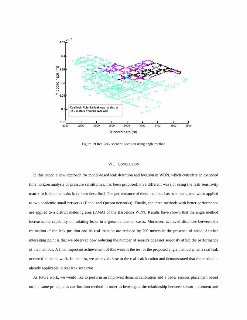
Figure 19 Real leak scenario location using angle method

VII. CONCLUSION

In this paper, a new approach for model-based leak detection and location in WDN, which considers an extended

time horizon analysis of pressure sensitivities, has been proposed. Five different ways of using the leak sensitivity

matrix to isolate the leaks have been described. The performance of these methods has been compared when applied

to two academic small networks (Hanoi and Quebra networks). Finally, the three methods with better performance

are applied to a district metering area (DMA) of the Barcelona WDN. Results have shown that the angle method

increases the capability of isolating leaks in a great number of cases. Moreover, achieved distances between the

estimation of the leak position and its real location are reduced by 200 meters in the presence of noise. Another

interesting point is that we observed how reducing the number of sensors does not seriously affect the performance

of the methods. A final important achievement of this work is the test of the proposed angle method when a real leak

occurred in the network. In this test, we achieved close to the real leak location and demonstrated that the method is

already applicable in real leak scenarios.

As future work, we would like to perform an improved demand calibration and a better sensors placement based

on the same principle as our location method in order to investigate the relationship between sensor placement and

the method used for leak location.

ACKNOWLEDGMENT

Authors would like to thank Gerard Sanz, phd student because for sharing with us the data necessary to perform

the real test presented in Section VI.C.

This work is supported by the Research Chair in Supervision and Advanced Control of Tecnológico de

Monterrey, Campus Monterrey and by a CONACYT studentship.

This work has been partially grant-funded by CICYT SHERECS DPI-2011-26243 and CICYT WATMAN DPI-

2009-13744 of the Spanish Ministry of Education and by iSense grant FP7-ICT-2009-6-270428 and by EFFINET

grant FP7-ICT-2012-318556 of the European Commission. of the European Commission.

REFERENCES

Casillas M.V., Garza L.E. and Puig V., Extended-Horizon Analysis of Pressure Sensitivities for Leak Detection in Water Distribution Networks,

8th IFAC Symposium on Fault Detection, Supervision and Safety of Technical Precesses, Safeprocess (2012), Mexico, p.570-575

Cheng, W. and He, Z. (2011). ”Calibration of Nodal Demand in Water Distribution Systems.” Journal of Water Resources Planning and

Management.,137(1), 31–40.

Colombo A., Lee P. and Karney B., A selective literature review of transient-based leak detection method, Journal of Hydro-environment

Research 2 (2009), p. 212-227

Covas D. and Ramos H., Hydraulic Transients used for Leak Detection in Water Distribution Systems, 4th International Conference on Water

Pipeline Systems, BHR Group, (2001), p. 227-241.

Ferrante M., Brunone B., Pipe system diagnosis and leak detection by unsteady-state tests. 1. Harmonic analysis, Advances in Water Resources,

Volume 26, Issue 1, January 2003a, Pages 95-105

Ferrante M., Brunone B., Pipe system diagnosis and leak detection by unsteady-state tests. 2. Wavelet analysis, Advances in Water Resources,

Volume 26, Issue 1, January 2003b, Pages 107-116

Fuchs H. V., Riehle R., Ten years of experience with leak detection by acoustic signal analysis, Applied Acoustics, 33 (1991), p. 1–19.

Fujiwara O. and Khang D. B., “A two-phase decomposition method for optimal design of looped water distribution networks,” Water Resources

Research, vol. 26, no. 4, pp. 539–549, 1990.

Goulet J.-A., Coutu S., Smith I.F.C., Model falsification diagnosis and sensor placement for leak detection in pressurized pipe networks, Journal

of Advanced Engineering Informatics, Volume 27, Issue 2, April 2013, Pages 261-269.

Herrera M., Torgo L., Izquierdo J., Pérez-García R., Predictive models for forecasting hourly urban water demand, Journal of Hydrology,

Volume 387, Issues 1–2, 7 June 2010, Pages 141-150

Kepler A., Covas D., Reis L. Leak detection by inverse transient analysis in an experimental PVC pipe system. Journal of Hydroinformatics. Vol

13 No. 2 (2011) p. 153-166

Koppel T., Vassiljev A., Use of modelling error dynamics for the calibration of water distribution systems, Journal of Advances in Engineering

Software, Volume 45, Issue 1, March 2012, Pages 188-196.

Mashford J., De Silva D., Marney D. and Burn S., An approach to leak detection in pipe networks using analysis of monitored pressure values by

support vector machine. Third International Conference on Network and System Security (2009), p. 534-539

Muggleton J.M., Brennan M.J., Pinnington R.J., Wavenumber prediction of waves in buried pipes for water leak detection, Journal of Sound and

Vibration 249 (5) (2002), p. 939–954.

Nicolini, M.; Patriarca, A., "Model calibration and system simulation from real time monitoring of water distribution networks," Computer

Research and Development (ICCRD), 2011 3rd International Conference on , vol.1, no., pp.51,55, 11-13 March 2011

Pérez R., Puig V., Pascual J., Quevedo J., Landeros E., Peralta A., Methodology for leakage location using pressure sensitivity analysis in water

distribution networks, Control Engineering Practice, Volume 19, Issue 10, October (2011a), p. 1157-1167.

Pérez R., Quevedo J., Puig V., Nejjari F., Cugueró M.A., Sanz G. and Mirats J.M., Leakage Location in Water Distribution Networks: a

Comparative Study of Two Methodologies on a Real Case Study, 19th Mediterranean Conference on Control Automation (2011b), Greece, p.

138-143

Pérez R., Puig V. and Pascual J., Leakage detection using pressure sensitivity analysis. Computing and Control in the Water Industry Conference

(2009a). Sheffield, UK.

Pérez, R., Puig, V., Pascual, J., Peralta, A., Landeros, E. and Jordanas, Ll. (2009b) “Pressure sensor distribution for leak detection in Barcelona

water distribution network”. Water Science & Technology , Vol 9 No 6 p. 715–721.

Quevedo, J., Pérez, R., Pascual, J., Puig, V., Cembrano, G., and Peralta, A. "Methodology to detect water losses in water hydraulic networks:

application to Barcelona water network", in Proc 8th IFAC International Symposium on Fault Detection, Supervision and Safety for Technical

Processes (SAFEPROCESS), Mexico City, MX, 2012, pp. 922-927.

Preis A., Whittle A., Ostfeld A., Perelman L., “Efficient Hydraulic State Estimation Technique Using Reduced Models of Urban Water

Networks.” Journal of Water Resources Planning and Management 137.4 (2011): 343Pudar S. and Ligget J., Leaks in Pipe Networks, Journal

of Hydraulics Engineering, 118 (7), (1992), p. 1031-1046.

Ragot J. and Maquin D., Fault measurement detection in an urban water supply network. Journal of Process Control, 16 (2006) 887–902.

Rossman L.A., Epanet 2 User’s Manual, Water Supply and Water Resources Division, Cincinnati, (2000).

Savic, D., Kapelan, Z., Jonkergouw, P. Quo vadis water distribution model calibration? Urban Water Journal, Vol. 6, No. 1 (2009). pp. 3-22.

Shu S., Zhang D, "Calibrating water distribution system model automatically by genetic algorithms," Intelligent Computing and Integrated

Systems (ICISS), 2010 International Conference on , vol., no., pp.16,19, 22-24 Oct. 2010.

Wu Z., Sage P., Turtle D. Pressure-Dependent Leak Detection Model and Its Application to a District Water System Journal of Water Resources

Planning and Management (2010) 136:1, p. 116-128.

Wu Z. et al., Leakage Detection via Hydraulic model calibration. Water Loss Reduction. Bentley Systems 2011.

Yang J., Wen Y., Li P., Leak location using blind system identification in water distribution pipeline, Journal of Sound and Vibration 310 (2008),

p. 134–148.