MODEL-BASED SENSOR SUPERVISION IN INLAND NAVIGATION NETWORKS: CUINCHY-FONTINETTES CASE STUDY. Dr. Joaquim Blesa (I) Dra. Klaudia Horváth (III), (IV) Dr. Eric Duviella (III), (IV) Dr. Vicenç Puig (I),(II) Dra. Yolanda Bolea (II) Dr. Lala Rajaoarisoa (III), (IV) Mrs. Karine Chuquet (V) (I) Institut de Robòtica I Informàtica Industrial (CSIC-UPC). Carrer Llorens Artigas, 4-

6, 08028 Barcelona, Spain. { joaquim.blesa,vicenc.puig}@upc.edu (II) Automatic Control Department, Universitat Politècnica de Catalunya, Pau

Gargallo, 5., 08003 Barcelona, Spain.+34 93 40179 17. yolanda.bolea@upc.edu

(III) EMDouai, IA, F-59500 Douai, France +33 3 27 71 21 02. {klaudia.horvath, eric.duviella, lala.rajaoarisoa}@mines-douai.fr

(IV) Univ Lille Nord de France, F-59000 Lille, France,

(V) VNF - Service de la navigation du Nord Pas-de-Calais, 37 rue du Plat, 59034 Lille Cedex, France. Karine.chuquet@vnf.fr

Abstract In recent years, inland navigation networks benefit from the innovation of the instrumentation and SCADA systems. These data acquisition and control systems lead to the improvement of the management of these networks. Moreover, they allow the implementation of more accurate automatic control to guarantee the navigation requirements. However, sensors and actuators are subject to faults due to the strong effects of the environment, aging, etc. Thus, before implementing automatic control strategies that rely on the fault-free mode it is necessary to design a fault diagnosis scheme. This fault diagnosis scheme has to detect and isolate possible faults in the system to guarantee fault-free data and the efficiency of the automatic control algorithms. Moreover, the proposed supervision scheme could predict future incipient faults that are necessary to perform predictive maintenance of the equipment. In this paper, a general architecture of sensor fault detection and isolation using model-based approaches will be proposed for inland navigation networks. It will be particularized for the Cuinchy-Fontinettes reach located in the north of France in order to show the effectiveness of the proposed fault diagnosis scheme. The preliminary results show the effectiveness of the proposed fault diagnosis methodologies using a realistic simulator and fault scenarios.

Keywords Inland Navigation Networks, Fault Diagnosis, interval models. Acknowledgements This work has been partially funded by grants CICYT SHERECS DPI-2011-26243 of Spanish Ministry of Education and by GEPET’Eau project which is granted by the French ministery MEDDE - GICC, the French institution ORNERC and the DGITM 1. INTRODUCTION The main management objective of the inland navigation networks is to guarantee the navigation in each reach (Blesa et al., 2012), i.e. the Normal Navigation Level (NNL). These levels are principally disturbed by the navigation and the lock operations. During lock operations, large volume of water is withdrawn from the upstream reach and supplied to the downstream reach causing a wave travelling in both directions; upstream to downstream, and downstream to upstream after reflection. To reduce the effect of wave and to maintain the NNL, it is necessary to control the gates which are generally located beside the locks. Another possibility is to control the discharges from natural rivers. The water levels are controlled by gates and measured by tele-operating sensors. To achieve these aims, an adaptive and predictive control architecture has been proposed in (Duviella et al., 2013) as depicted in Figure 1. This architecture is based on a SCADA system allowing the tele-control of the navigation network. A Human Machine Interface (HMI) is dedicated to the supervision of the inland navigation network by a supervisor. The management constraints and rules are gathered in the Management Objectives and Constraints Generation module (MOCG). To perform the management of the inland navigation network, a Hybrid Control Accommodation module (HCA) allows the determination of set-points (Management Strategies block) according to the current state (Supervision block) and the forecasting of the future state (Prognosis block) of the network. These strategies can be adapted or improved according to the Decision Support module (DS).

Figure 1- Inland navigation network adaptive and predictive control architecture.

In this work, we will focus on the part of the supervision block that determines if a sensor fault is present in the system (detection) and identifies what sensor is affected by the fault (isolation). In particular, model-based fault diagnosis techniques will be used for the implementation of the sensor supervision block. 2. MODEL-BASED FAULT DETECTION AND ISOLATION The principle of model-based fault detection is to test whether the measured input and output from the system lie within the behavior described by a model of the faultless system. If the measurements are inconsistent with the model of the faultless system, the existence of a fault is proved. In general, two different types of models can be distinguished: qualitative and quantitative models. Quantitative models are used in the Systems Dynamics and Control Engineering community (Gertler, 1998; Iserman, 2006; Blanke et al., 2006; Ding, 2008) known as FDI (Fault Detection Isolation) community. Quantitative models are mathematical models that can be described in time or frequency domains and most of the fault detection techniques based on this kind of models uses a residual that describes the consistency check between the predicted, obtained by the model, and the real behaviour, y(k) measured by the sensors. This fault detection approach is known as based on analytical redundancy. 2.1 ROBUST FAULT DETECTION

Ideally, in quantitative model-based fault detection methods residuals should only be affected by the faults. However, the presence of disturbances, noise and modelling errors causes residuals to become nonzero in the absence of faults and thus interferes with the detection of faults. Therefore, the fault detection procedure must be robust against these undesired effects (Chen and Patton, 1999) . In case parametric uncertainties are taken into account, the healthy system model should include a vector of uncertain parameters bounded by sets that contain all possible parameter values when the system operates normally. One of the most developed families of approaches, called active, is based on generating residuals which are insensitive to uncertainty, while at the same time sensitive to faults. This approach has been extensively developed by several researchers using different techniques: unknown input observers, robust parity equations, etc. In the book of Chen and Patton (1999), there is an excellent survey of this active approach. On the other hand, there is a second family of approaches, called passive (Puig et al., 2008), which enhances the robustness of the fault detection system at the decision-making stage. 2.2 INTERVAL MODEL Let us assume that the system to be monitored can be modeled using a model which is linear in the parameters that can be expressed in discrete time regressor form, Moving Average (MA) model as follows:

ˆ( ) ( , ) ( ) ( ) ( )y k k e k y k e k= τ + = +φ θ (1)

where

- ( , )k τφ is the regressor vector of dimension 1 nθ× which can contain any function of

inputs ( )ku and output ( )y k .

- τ is the transport delay that is unknown but belong to a set of natural numbers:

{ }0 0 0, 1,τ τ ττ τ λ τ λ τ λ∈ − − + + with 0 , ττ λ ∈ and 0ττ λ>

- ∈θ Θ is the parameter vector of dimension 1nθ × .

- Θ is the set that bounds parameter values. In particular, for interval models, the set of uncertain parameters is bounded by an interval box centered in the nominal parameter values: 1 1, ,n nθ θ

θ θ × × θ θ Θ where: 0

i i iθ θ −λ; 0

i i iθ θ + λ i=1,…, nθ , being 0

iθ the nominal parameter values; - ( )e k is the additive error bounded by a constant ( )e k ≤ σ .

The parameter set Θ and additive error bound σ are calibrated using fault-free data from the system (rich enough regarding the identification point of view) and in such a way that all measured data in a fault-free scenario will be covered by the interval predicted output produced by using model (1), that is

ˆ ˆ( ) ( ) , ( )y k y k y k ∈ −σ + σ (2)

where

{ }( )

{ }( )

0 0 0

0 0 0

, , 1,

, , 1,

ˆ ( ) max ( , )

ˆ( ) min ( , )

y k k

y k kτ τ τ

τ τ τ

τ τ λ τ λ τ λ

τ τ λ τ λ τ λ

τ

τ

∈ ∈ − − + +

∈ ∈ − − + +

=

=

θ Θ

θ Θ

φ θ

φ θ

(3)

One of the key points in model based fault detection is how models are built and their uncertainty is estimated. The structure of the model, determined by ( , )k τφ and θ , nominal parameters 0θ and nominal transport delay 0τ can be obtained by the physical knowledge of the system or by conventional identification techniques (Ljung, 1999). The additive error bound σ can be computed by a noise study. The delay uncertainty τλ can be determined considering that the input process signal is white noise and

carrying out the study of the independence between the input and output process signals using confidence intervals (usually, 99% or 95%). On the other hand, given N measurements of outputs and inputs from a scenario free of faults and rich enough from the identifiability point of view, the uncertainty in parameters ( iλ i=1,…, nθ ) can by computed by solving an optimization problem (Blesa et al, 2010). 2.3 FAULT DETECTION

Once model (1) has been calibrated in a non-faulty scenario, it can be used for fault detection checking if

( ) ( )y k k∉ϒ (4)

where ( )kϒ is the direct image of the uncertain model defined as

{ }{ }0 0 0ˆ ˆ( ) ( ) | ( ) ( , ) , , , , 1,

ˆ ˆ ( ) , ( )

k y k e y k k e

y k y k

τ τ τ τϒ = + = ∈ ≤ σ τ∈ τ −λ τ −λ + τ + λ =

= −σ + σ

φ θ θ Θ

(5)

In case that (4) is proved, a fault can be indicated, otherwise no fault can be indicated. Equivalently, the fault detection test (4) can be formulated in terms of the residual defined as

ˆ( ) ( ) ( ) ( ) ( ) ( , ) ( )r k y k y k e k y k k e kτ= − − = − −φ θ (6)

Residual (6) corresponds to a MA parity equation (Gertler, 1998). Ideally, when modeling errors and noise are neglected, residual (6) should be zero in a fault-free scenario and different from zero, otherwise. However, because of modeling errors and noise, residuals can be different from zero in a non-faulty scenario. In order to take into account uncertainty in parameters and additive noise, the effects of these uncertainties will be propagated to the residuals defining the region of admissible residuals. A fault will be detected when zero does not belong to this set. Thus, the fault detection test is equivalent to check the following condition

0 ( )k∉Γ (7)

where ( )kΓ is the interval of possible residuals defined as follows

{ }{ }0 0 0( ) ( ) | ( ) ( ) ( , ) , , , , 1,k r k r k y k k e eτ τ τ τΓ = = − − ∈ ≤ σ τ∈ τ −λ τ −λ + τ + λφ θ θ Θ (8)

This test based on the direct evaluation of the residual is known as the direct test (Blesa et al., 2011). 2.4 FAULT ISOLATION Fault isolation consists in identifying the faults affecting the system once a fault has been detected. Fault isolation could be carried out, as classically proposed in FDI books (Gertler, 1998 and Isermann, 2006, among others). Given a set of nr residuals { }1( ), , ( )

rnr k r k at time k, the fault detection tests (4) or (7) applied component-wise to each single residual

0 if ( ) is consistent( )

1 if ( ) is not consistenti

ii

r kk

r k

φ =

(9)

produces the observed fault signature ( )kφ :

( )1 2( ) ( ), ( ), , ( )rnk k k k= φ φ φφ (10)

The observed fault signature is, then, supplied to the fault isolation module that has the knowledge about the binary relation between the considered fault hypothesis set

{ }1 2( ) ( ), ( ), , ( )fnk f k f k f k= f (11)

and the fault signal set ( )kφ . This relation is stored in the called theoretical binary fault signature matrix (FSM) of dimension r fn n× . Thereby, an element FSMi,j of this matrix is equal to 1 if the fault hypothesis fj(k) is expected to affect the residual ri(k) such that the related fault signal fi(k) is equal to 1 when this fault is affecting the monitored system. Otherwise, the element FSMi,j is zero-valued.

Considering single faults, a general approach of carrying out the isolation is comparing the observed fault signature ( )kφ with the theoretical one related to every fault hypotheses that can be calculated as the distance between both vectors: ( )kφ and the jth-column of matrix FSM for the hypothesis fj, e.g. using the Hamming distance measurement. As a result of this comparison, a distance measurement disj(k) is obtained for every fault hypothesis fj, being dis(k) the vector of all the computed distances at time instant k: ( )1( ) ( ), , ( ), , ( )j nfk dis k dis k dis k= dis . If the Hamming distance approach is applied, then

( ) ( )( ),1

( ) FSM XOR ( )rn

j i j ii

dis k k=

= φ∑ (12)

where XOR is the XOR logic operator. Then, the fault hypotheses with the shortest distance regarding the current observed fault signature ( )kφ are considered as the fault isolation result:

{ }1, ,: if ( ) min ( )j j nf

f dis k dis kνν∈

= ∈ =

DGN

f (13)

where DGN is the set of fault hypothesis fj which are consistent with the observed fault signals. 3. INLAND NAVIGATION MODEL

Figure 2-Piece of Inland navigation network of the north of France and its Scheme

The real behaviour of every reach NR i of the network, can be described by the Saint-Venant (SV) equations (Chow, 1959) are partial-differential equations that describe accurately the dynamics in a one-dimensional free surface flow. These equations express the conservation of mass and momentum principles in a one-dimensional free surface flow:

0Q Sx t

∂ ∂+ =

∂ ∂ .

( )2

0Q Q hgS gS I Jt x S x

∂ ∂ ∂+ + − − =

∂ ∂ ∂ (14)

where ( , )Q Q x t= is the flow (in m3/s), ( , )S S x t= is the cross-sectional area (in m2), t is the time variable (in s), x is the spatial variable (in m), measured in the direction of the movement, h is the spatial variable corresponding to the water elevation (in m), g is the gravity (in m/s2), I is the bottom slope and J is the friction slope.

Since there is no known analytical solution for equations (14) in real geometry, they have to be solved numerically. Then, the hydraulic behavior of this canal system can be studied through numerical methods. Because of the complexity and the computational load of this complete distributed model several simplified models have been deduced from the SV equations with different simplifications (Bolea et al., 2014), for example the IDZ model (Litrico and Fromion, 2004). The IDZ model is based on the linearisation of the SV equations around a set-point (in this case given by the NNL), the canal reach is divided into two parts: an upstream (uniform flow) part and a downstream (backwater) part. The relation between the level and the flow in these two parts is given by the following transfer function

1 11 21 1

2 12 22 2

( ) ( )( ) ( )

y s G G q sy s G G q s

=

(15)

where: y1 and y2 for levels and q1, and, q2 for flows denote upstream/downstream

deviations from stationary values, 1111

1

1( )

p sG sA s+

= , 21

1221

1( )

sp eG sA s

τ−−= ,

1221

122

( )sp eG s

A s

τ−+=

and 2222

2

1( )

p sG sA s

−= . Discretizing (15) using a sample time Ts, the following MA models

can be obtained 1 1 1 1

1 1 1,1 1 1,2 1 2,1 2 21 2,2 2 21 1

2 2 2 22 2 1,1 1 12 1,2 1 12 2,1 2 2,2 2 2

( ) ( 1) ( ) ( 1) ( ) ( 1) ( )

( ) ( 1) ( ) ( 1) ( ) ( 1) ( )

y k y k b q k b q k b q k b q k e k

y k y k b q k b q k b q k b q k e k

τ τ

τ τ

= − + + − + − + − − +

= − + − + − − + + − + (16)

In inland navigation reaches, there can exist intermediate measurement levels and intermediate points were extra flows can be injected/extracted. Then, in a general case a reach with yn measurement level points and with qn input/output flow points, the following model can be

( ),1 , ,2 ,1

( ) ( 1) ( ) ( 1) ( )qn

i ii i j j j i j j j i i

jy k y k b q k b q k e kτ τ

=

= − + − + − − +∑ 1, , yi n= (17)

that can be rewritten as ( ) ( , ) ( )i i i i iy k k e k= +φ θτ 1, , yi n= (18)

with

( )1 1, 1 1, ,( , ) ( 1), ( ), ( 1), , ( 1)q qi i i i i n n ik y k q k q k q k= − − τ − τ − − τ −φ τ (19)

( )1,1 1,2 ,21, , , ,q

Ti i ii nb b b=θ (20)

Since the IDZ is a physical-based model with a given structure, determined by ( , )i ikφ τ and iθ 1, , yi n= in (18), nominal parameters 0

iθ and nominal delays 0iτ are given by

the physical knowledge of the system (Litrico and Fromion, 2004). Finally, given input/output data from a scenario free of faults and rich enough from the identifiability point of view, the uncertainty in parameters and time delays around their nominal values can be estimated. 4. FAULT DETECTION AND ISOLATION SCHEME Considering a navigation reach, described by (17), with yn measurement level points and

qn input/output flow points, yn different sensor faults can be defined ( ) ( ) ( )nf

i i iy k y k f k= + 1, , yi n= (20) where ( )nf

iy k is the real value of the level i and and ( )if k the additive error fault that affects to level sensor i. Thus, yn primary residuals can be obtained as follows

( ) ( , ) ( )i i i i i ir y k k e k= − −φ θτ 1, , yi n= (21) Once the interval model has been calibrated, consistency test (7) can be applied to every residual (21). Regarding the fault isolation, considering the yn residuals affected by the possible

yn faults, the Fault Signature Matrix defined in Table 1 can be obtained.

Table 1- Fault Signature Matrix of residuals system (21) 1f 2f

1nyf − nyf

1r 1 0 0 0 0 2r 0 1 0 0 0 0 0

0 0 1nyr − 0 0 0 1

nyr 0 0 0 0 1

The problem of using model (17) in (21) for generating residuals, that allow sensor fault detection, is that it behaves as a dead-beat observer which can only indicate a fault for a minimum time period given by the system order. This implies that after a number of samples (related to the order of the system) once the fault has appeared, the residual tends to be small even the fault still is present (Ding, 2008). In order to deal with this problem, when an inconsistency is detected in residual ir at instant fk a new residual

_ 2ir is activated for fk k>

_ 2ˆ( ) ( ) ( )i i ir k y k y k= − 1, , yi n= (21)

with ˆ ( )iy k obtained by the following mass-balance average simulation model 1ˆ ˆ( ) ( 1) ( )i i iy k y k Q kA

= − + (22)

where A is the longitudinal area of the reach and the input average flow ( )iQ k is computed as 1

,1 H

( ) ( )qn k

i l l il j k

Q k q j−

= = −

= − τ∑ ∑ (23)

and the initial condition of the simulation model is given by 1

H

ˆ ( ) ( )j kf

i f ij kf

y k y j= −

= −

= ∑ (24)

Then, the fault signature component ( )i kφ will be activated while the residual _ 2 ( )ir k will be bigger or equal a threshold _ 2iσ , i.e.,

_ 2 _ 2

_ 2 _ 2

0 if ( )( )

1 if ( )

i i

i

i i

r kk

r k

σ

σ

≤φ = >

(25)

where _ 2iσ 1, , yi n= are the detection threshold calibrated in a fault-free scenario. 5. CUINCHY FONTINETTES REACH The Cuinchy-Fontinettes Reach (CFR) has a crucial importance due to its localization, between two major catchment areas and its size (more than 40 km long). The main use of the CFR is for navigation purposes. However, it can be used to stock water volumes during wet periods in order to avoid or to limit floods in the two catchment areas, and during dry period to supply water to these two areas. The CFR is located between the upstream lock of Cuinchy at the East of the town Bethune and, at the Southwest of the town Saint-Omer, the downstream lock of Fontinettes (see Figure 3). The first part of the channel corresponds to the 28.7 km from Cuinchy to Aire-sur-la-Lys. The second part of the channel corresponds to 13.6 km from Aire-sur-la-Lys to Fontinettes. The channel is entirely artificial and has no significant slope. Considering the navigation flow, the water runs off from Cuinchy to Fontinettes. There are 3 measurement points in Cuinchy, Aire-sur-la-Lys and Fontinettes. The input/output flow points are located in:

• Cuinchy: where the flow can be injected by the lock operation (activated by navigation rules) and a submerged gate that can supply a controlled flow.

• Aire: where the flow can be injected/extracted by a controlled gate. • Fontinettes: where the flow can be extracted by the lock operation (activated by

navigation rules).

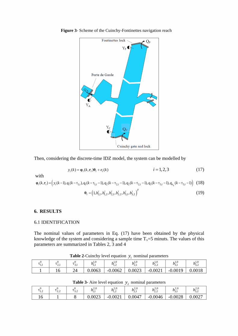
Figure 3- Scheme of the Cuinchy-Fontinettes navigation reach

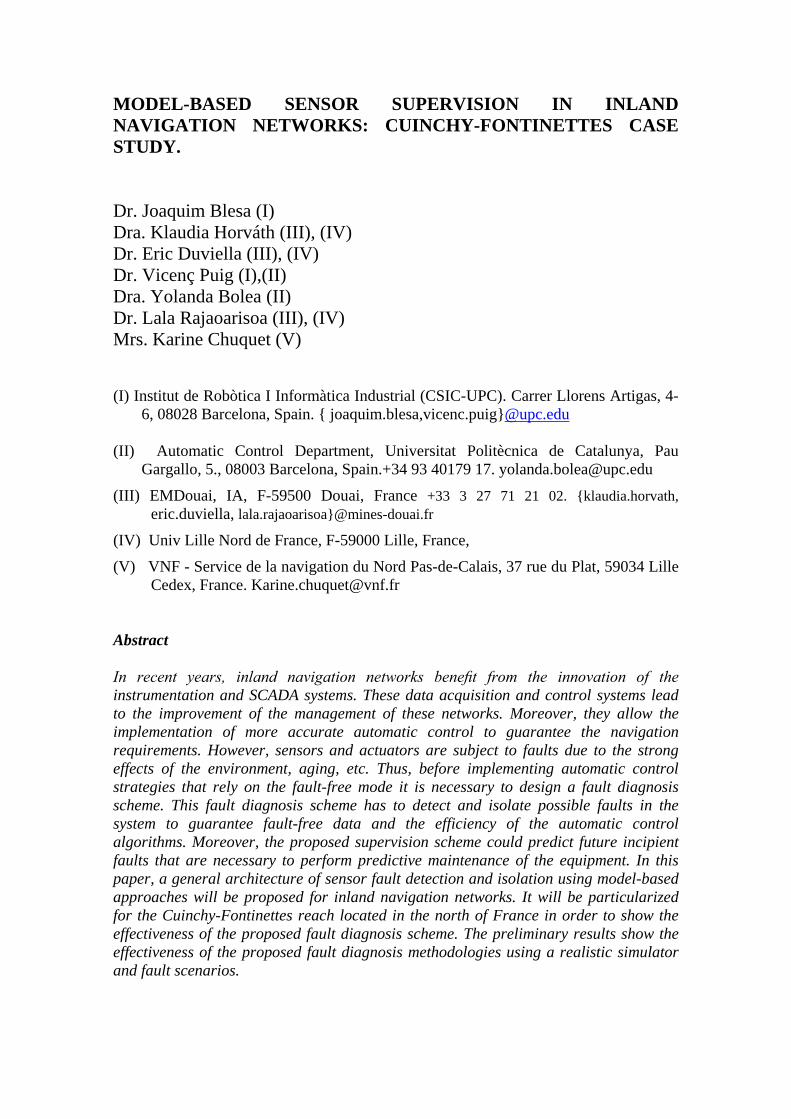
Then, considering the discrete-time IDZ model, the system can be modelled by

( ) ( , ) ( )i i i i iy k k e k= +φ θτ 1, 2,3i = (17) with

( )1 1, 1 1, 2 2, 2 2, 3 3, 3,( , ) ( 1), ( ), ( 1), ( 1), ( 1), ( 1), ( 1)qi i i i i i i i n ik y k q k q k q k q k q k q k= − − τ − τ − − τ − − τ − − τ − − τ −φ τ (18)

( )1,1 1,2 2,1 2,2 3,1 3,21, , , , , ,Ti i i i i i

i b b b b b b=θ (19) 6. RESULTS 6.1 IDENTIFICATION The nominal values of parameters in Eq. (17) have been obtained by the physical knowledge of the system and considering a sample time Ts=5 minuts. The values of this parameters are summarized in Tables 2, 3 and 4

Table 2-Cuinchy level equation 1y nominal parameters 01,1τ 0

2,1τ 03,1τ 1,0

1,1b 1,01,2b 1,0

2,1b 1,02,2b 1,0

3,1b 1,03,2b

1 16 24 0.0063 -0.0062 0.0023 -0.0021 -0.0019 0.0018

Table 3- Aire level equation 2y nominal parameters 01,2τ 0

2,2τ 03,2τ 2,0

1,1b 2,01,2b 2,0

2,1b 2,02,2b 2,0

3,1b 2,03,2b

16 1 8 0.0023 -0.0021 0.0047 -0.0046 -0.0028 0.0027

Table 4- Fontinettes level equation 3y nominal parameters 01,3τ 0

2,3τ 03,3τ 3,0

1,1b 3,01,2b 3,0

2,1b 3,02,2b 3,0

3,1b 3,03,2b

24 8 1 0.0019 -0.0018 0.0028 -0.0027 -0.0042 0.0040 Once the nominal parameters have been computed, a fault-free scenario has been generated by numerical model implemented in the SIC (Simulation Irrigation Canals) software (Malaterre, 2006). SIC uses a finite difference method to solve the SV equations implicitly. The fault-free scenario defined by the input (positive) and output (negative) flow values in 6 days , based on a realistic scenario is depicted in Figure 4. Using this fault-free scenario and solving optimization problems (Blesa et al., 2010; Puig and Blesa, 2013) the uncertainty in parameters has been computed in such a way that the non faulty data is contained in the interval bounds following Eq. (2) .

Figure 4- Input(positive)/output(negative) flow values in the fault-free scenario

The uncertain bounds in parameters obtained in the identification procedure are the following

- Delay uncertainty: 2τλ = for all the transport delays - Additive errors: 1 1,5cmσ = , 2 3cmσ = and 3 3.5cmσ = - Uncertainty in parameters: ( )1 1,0

, 1 ,1i j i jb b= ±α , ( )2 2,0, 2 ,1i j i jb b= ±α and ( )3 3,0

, 3 ,1i j i jb b= ±α with 1 0.066α = , 2 0.027α = and 3 0.008α =

Figure 5 shows the evolution of the Cuinchy, Aire and Fontinettes levels and the bound levels obtained using the interval model.

Figure 5- Levels and interval bound levels in the fault-free scenario

6.2. FAULT DETECTION

Once the interval model has been calibrated, different fault scenarios have been simulated in order to verify the effectiveness in fault detection using Test (4) or (7). Figure (6) shows the evolution of the bounds of the interval residuals 1Γ in the Cuinchy level when an additive fault of -2cm has been introduced in this sensor level i.e

1 0.02f m= − at 990fk = (i.e. at time 82h 30’). Figure 7 depicts the details of Figure 6 around the fault time occurrence.

Figure 6- Bounds of the interval residuals 1Γ (Cuinchy level residual)

Figure 7- Detail of bounds of the interval residuals 1Γ (Cuinchy level residual)

Finally, Figure 8 (upper) shows the fault detection results applying fault detection test defined in Eq. (7) to 1r and (lower) applying this fault detection test but with the additional residual 1_ 2r defined in Eq. (23) in order to deal with the dead-beat observer effect described in Section 4. As can be seen if test (7) is directly applied to 1r there is not persistence in the fault indicator, whereas that this problem disappear when the auxiliary residual is used and there is persistence in the fault indicator.

Figure 8- Fault detection results without and with additional residual 1_ 2r

6. CONCLUSIONS

In recent years, inland navigation networks have benefited from the innovation of the instrumentation and SCADA systems. However, before implementing automatic control strategies that rely on the fault-free mode it is necessary to design a fault diagnosis scheme. In this paper, a model-based scheme has been proposed for the sensor level fault detection and isolation in inland navigation networks. The scheme is based on the use of analytical redundancy provided by a mathematical model. The fault detection is implemented by a passive robust approach based on interval methods that consider uncertainty in parameters of the mathematical model and additive error. Finally, the proposed scheme has been successfully validated in real scenarios using a high-fidelity simulator of a reach of the inland navigation network located in the north of France. BIBLIOGRAPHY Blanke M, Kinnaert M, Lunze J, Staroswiecki M, Schröder J. Diagnosis and Fault-Tolerant Control. Springer-Verlag: New York; 2006 Blesa J, Puig V, Bolea Y. Fault detection using interval LPV models in an open-flow canal. Control Engineering Practice 2010; 18(5), 460-470. Blesa J, Puig V, Saludes J. Identification for passive robust fault detection using zonotope-based set-membership approaches. International Journal of Adaptive Control and Signal Processing 2011; 25 (9): 788–812. Blesa J, Duviella E, Sayeb-Mouchaweh M, Puig V, Chuquet K. Automatic Control To Improve The Seaworthiness Conditions In Inland Navigation Networks. Journal of Maritime Research 2012; 9(3): 61-66. Bolea Y, Puig V, Blesa J. Linear parameter varying modeling and identification for real-time control of open-flow irrigation canals. Environmental modelling & software 2014; 53. 87-97 Chen J, Patton R.J. Robust Model-Based Fault Diagnosis for Dynamic Systems. Kluwer Academic Publishers: Dordrecht; 1999. Chow V.T. Open-channel hydraulics, McGraw-Hill. New York; 1959. Ding S.X. Model-based Fault Diagnosis Techniques Design Schemes, Algorithms, and Tools. Springer: Berlin; 2008. Duviella E, Rajaoarisoa L, Blesa J, Chuquet K. Adaptive and predictive control architecture of inland navigation networks in a global change context: application to the Cuinchy-Fontinettes reach. IFAC Proceedings Volumes (IFAC-PapersOnline): 7th IFAC Conference on Manufacturing Modelling, Management, and Control, MIM 2013; Saint Petersburg; Russian Federation; 19 June 2013 through 21 June 2013. 2201-2206. Gertler, J. Fault Detection and Diagnosis in Engineering Systems. Marcel Dekker: New York. 1998. Horváth K, Duviella E, Blesa J, Rajaoarisoa L, Bolea Y, Puig V, Chuquet K. Gray-box model of inland navigation channel: Application to the Cuinchy-Fontinettes reach. Journal of Intelligent Systems 2014 In press (DOI: 10.1515/jisys-2013-0071)

Isermann R. Fault-diagnosis systems: An introduction from fault detection to fault tolerance. Springer: Berlin; 2006. Litrico X, Fromion V. Simplified modeling of irrigation canals for controller design. Journal of Irrigation and Drainage Engineering 2004; 130(5):373–383. Ljung L. System identification–theory for the user (2nd ed.). Englewood Cliffs, NJ: Prentice-Hall; 1999. Malaterre P.O. Sic 5.20, simulation of irrigation canals, 2006. URL: http://www.canari.free.fr/sic/sicgb.htm Puig V, Quevedo J, Escobet T, Nejjari F, de las Heras S. Passive Robust Fault Detection of Dynamic Processes using Interval Models. IEEE Transactions on Control Systems Technology 2008; 16 1083–1089. Puig V, Blesa J. Limnimeter and rain gauge FDI in sewer networks using an interval parity equations based detection approach and an enhanced isolation scheme. Control Engineering Practice 2013; 21(2): 146-170.